Public Choice (2010) 142: 69–90DOI 10.1007/s11127-009-9475-2

Determinants of the probability and timingof commercial casino legalization in the United States

Peter T. Calcagno · Douglas M. Walker ·John D. Jackson

Received: 2 June 2008 / Accepted: 18 June 2009 / Published online: 1 July 2009© Springer Science+Business Media, LLC 2009

Abstract The adoption of lotteries by state governments has received significant attention inthe economics literature, but the issue of casino adoption has been neglected by researchers.Casino gambling is a relatively new industry in the United States, outside Nevada and NewJersey. As of 2007, 11 states had established commercial casinos; several more states areconsidering legalization. We analyze the factors that determine a state’s decision to legalizecommercial casinos, using data from 1985 to 2000, a period which covers the majorityof states that have adopted commercial casinos. We use a tobit model to examine states’fiscal conditions, political alignments, intrastate and interstate competitive environments,and demographic characteristics, which yields information on the probability and timing ofadoptions. The results suggest a public choice explanation that casino legalization is due tostate fiscal stress, to efforts to keep gambling revenues (and the concomitant gambling taxes)within the state, and to attract tourism or “export taxes.”

Keywords Casinos · Casino adoption · Legalized gambling · Fiscal stress · Tax revenues

JEL Classification D72 · L83 · H7

1 Introduction

Prior to 1989 commercial casino gambling was legal only in Nevada and New Jersey. Nevadalegalized casinos in 1931, and casinos opened in Atlantic City, NJ, in 1978. With the U.S.

Earlier versions of this paper were presented at the 2008 Southern Economic Association and 2008Association of Private Enterprise Education. We would like to thank the participants in those sessionsfor their helpful comments. We would also like to thank the participants of the College of CharlestonDepartment of Economics and Finance Seminar Series. Finally, we would like to acknowledgethe anonymous referees from whose comments we greatly benefited. The usual caveats apply.

P.T. Calcagno (�) · D.M. WalkerCollege of Charleston, Charleston, SC 29424-0001, USAe-mail: calcagnop@cofc.edu

J.D. JacksonAuburn University, Auburn, AL 36849, USA

70 Public Choice (2010) 142: 69–90

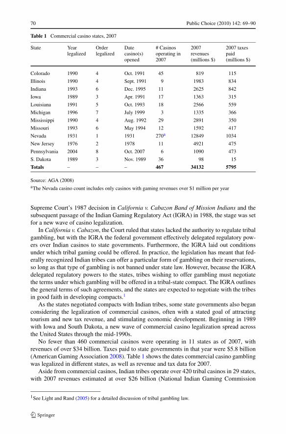
Table 1 Commercial casino states, 2007

State Yearlegalized

Orderlegalized

Datecasino(s)opened

# Casinosoperating in2007

2007revenues(millions $)

2007 taxespaid(millions $)

Colorado 1990 4 Oct. 1991 45 819 115

Illinois 1990 4 Sept. 1991 9 1983 834

Indiana 1993 6 Dec. 1995 11 2625 842

Iowa 1989 3 Apr. 1991 17 1363 315

Louisiana 1991 5 Oct. 1993 18 2566 559

Michigan 1996 7 July 1999 3 1335 366

Mississippi 1990 4 Aug. 1992 29 2891 350

Missouri 1993 6 May 1994 12 1592 417

Nevada 1931 1 1931 270a 12849 1034

New Jersey 1976 2 1978 11 4921 475

Pennsylvania 2004 8 Oct. 2007 6 1090 473

S. Dakota 1989 3 Nov. 1989 36 98 15

Totals – – – 467 34132 5795

Source: AGA (2008)aThe Nevada casino count includes only casinos with gaming revenues over $1 million per year

Supreme Court’s 1987 decision in California v. Cabazon Band of Mission Indians and thesubsequent passage of the Indian Gaming Regulatory Act (IGRA) in 1988, the stage was setfor a new wave of casino legalization.

In California v. Cabazon, the Court ruled that states lacked the authority to regulate tribalgambling, but with the IGRA the federal government effectively delegated regulatory pow-ers over Indian casinos to state governments. Furthermore, the IGRA laid out conditionsunder which tribal gaming could be offered. In practice, the legislation has meant that fed-erally recognized Indian tribes can offer a particular form of gambling on their reservations,so long as that type of gambling is not banned under state law. However, because the IGRAdelegated regulatory powers to the states, tribes wishing to offer gambling must negotiatethe terms under which gambling will be offered in a tribal-state compact. The IGRA outlinesthe general terms of such agreements, and the states are expected to negotiate with the tribesin good faith in developing compacts.1

As the states negotiated compacts with Indian tribes, some state governments also beganconsidering the legalization of commercial casinos, often with a stated goal of attractingtourism and new tax revenue, and stimulating economic development. Beginning in 1989with Iowa and South Dakota, a new wave of commercial casino legalization spread acrossthe United States through the mid-1990s.

No fewer than 460 commercial casinos were operating in 11 states as of 2007, withrevenues of over $34 billion. Taxes paid to state governments in that year were $5.8 billion(American Gaming Association 2008). Table 1 shows the dates commercial casino gamblingwas legalized in different states, as well as revenue and tax data for 2007.

Aside from commercial casinos, Indian tribes operate over 420 tribal casinos in 29 states,with 2007 revenues estimated at over $26 billion (National Indian Gaming Commission

1See Light and Rand (2005) for a detailed discussion of tribal gambling law.

Public Choice (2010) 142: 69–90 71

2008). Casino gambling has become one of the most popular forms of entertainment, and isamong the fastest growing service industries in the United States. Yet, its growth is tightlycontrolled by state governments.2 Concerns about the current U.S. recession, as well asstate-level fiscal crises, may explain why more than 14 states are considering proposals toallow or expand slot machines or casinos (Bluestein 2009). If economic conditions in theUnited States continue to worsen, this list of states is likely to grow.3

While it may seem obvious why so many states have legalized, or are considering le-galizing casinos, there have been very few analyses of the casino adoption decision. Thereare many reasons and questions associated with casino adoption by state governments. Is itsimply fiscal stress or a desire for alternative revenue sources that explains the adoption ofcasinos? Is it an effort to keep casino customers—and the tax revenues—within the state?Are casinos adopted to spur economic development and job growth? Or are casinos legal-ized simply to provide consumers with another entertainment option? Our purpose in thispaper is to examine the different factors that lead to casino adoption at the state level. Theanalysis utilizes a random effects tobit model estimated with panel data from 1985 to 2000,a period that covers the era during which all casino legalization has occurred outside Nevadaand New Jersey.4 We consider a number of fiscal, political party, gambling competition, anddemographic variables in an attempt to determine which factors affect the timing and prob-ability of casino adoption. The paper is organized as follows. Section 2 is a review of theliterature. In Sect. 3 we discuss the data and the model. Section 4 presents the results anddiscussion, and Sect. 5 concludes.

2 Review of the gambling adoption literature

Little research attention has been paid to decisions to adopt casino gambling. This is sur-prising considering the size of the industry and the intensity of debate over casino expan-sion. Researchers have examined economic development effects from casinos in particularjurisdictions, the relationships between different forms of gambling, and the social costsattributable to legalized gambling. To be sure, there is a large and growing body of gam-bling research.5 However, the factors affecting the decision to adopt casinos have almostcompletely been ignored in the economics literature.

2Our focus in this paper is on the decision to legalize commercial casinos, because this is an autonomousdecision on the part of the state governments. Hereafter, when we refer to “casinos,” we mean commercialcasinos, unless otherwise indicated. It is important to note that not all casinos are created equal. The mega-casino resorts in Nevada and Atlantic City are very different from casinos in many other states. For example,casinos in Colorado are very small and have strict betting limits ($5). Casinos in Kansas City, Missouri tendto cater to “day-trippers,” and are not destination resorts. States regulate almost every aspect of casinos: thenumber to be allowed, their size, the types of games allowed, maximum bets, entry fees, etc. Casino legaliza-tion proposals are specific on these criteria, and passage is surely dependent on them. Although beyond thescope of this paper, these issues would be interesting topics for future research.3Richburg (2008) reports that “at least 13 states are facing huge shortfalls for the next fiscal year, and abouthalf a dozen others are in serious financial difficulty.”4The only exception is very recent: Pennsylvania opened its first stand-alone casino in late 2007. However, itonly offers slot machines.5See Walker (2007) for a comprehensive overview of the gambling literature.

72 Public Choice (2010) 142: 69–90

2.1 Casino adoption

Furlong (1998) is the one paper of which we are aware that examines the casino adop-tion question.6 He lists four general motivations for the legalization of casinos: (1) “Therevenue rationale”—legalize to raise tax revenues; (2) “The political rationale”—gamblingtaxes may be preferred to other types of taxes or decreased government spending; (3) “Thecompetitive rationale”—states adopt in order to compete for tax revenues with nearby states;and (4) “The economic development rationale”—casinos may stimulate local and state-levelgrowth.

Furlong performs a cross-sectional analysis of adoption, with a dichotomous variableto indicate whether a state has legalized casinos. His analysis excludes Alaska and Hawaiibecause of missing data, and Nevada and New Jersey are excluded because they adoptedcasinos much earlier than other states. As a result, there are seven “adopting” states, and39 “non-adopting” states. In order to test which variables explain adoption, Furlong usesbivariate logistic regressions. He then posits a multivariate model based on the bivariateresults that appeared promising. Furlong finds that the political and economic developmentrationales are supported by the empirical results, but he finds no evidence for the revenueand competitive rationales.

The analysis by Furlong has a number of limitations. First, it utilizes cross-sectional butnot time-series data, so the model ignores the timing of the adoption decision as it relatesto changes in the explanatory variables.7 Second, much of the data used by Furlong areoutdated; his most recent observation on explanatory variables are from 1990, prior to thelegalization decision by most of the states in his model. Third, Furlong uses only four ex-planatory variables in his full model; clearly, there is a concern about omitted variable bias.Despite these limitations, Furlong’s discussion and results are informative.

2.2 Lottery adoption

Although there has been little research attention on casino adoption, lotteries have receivedmuch attention. New Hampshire was the first state of the modern gambling era to adopt alottery, in 1964. Currently 44 states have lotteries, with total sales exceeding $60 billionin 2008,8 about 50% of which is retained by the state governments to cover expenses andsupplement state coffers (Garrett 2001).

Many facets of lotteries have been examined by economists, from the regressivity of thelottery “tax,” to the contributions of lottery taxes to ear-marked programs (e.g., college tu-ition subsidies). Another key area of inquiry has been the states’ decisions to adopt lotteriesand the timing of adoption. As lotteries and casinos have the potential to raise significanttax revenues, the lottery literature has an obvious parallel to our study. Since there has beenvery little published on the casino adoption question, we use the relevant papers from thelottery literature as a guide.

6Sirakaya et al. (2005) focus on predicting outcomes of county referenda on casino legalization using anartificial neural network. Their focus is primarily on the demographic factors that explain individuals’ supportfor casinos at the community level. In contrast, our concern in this paper is with legislative preferences andstate-level casino adoption decisions.7Some of Furlong’s variables can be seen as measuring change through time. However, dividing a variable’s1990 value by its 1970 value, as Furlong does to calculate the change in per capita taxes, does not give muchdetail on how the variable has changed through time, especially as such changes relate to the timing of casinoadoptions.8Source: North American Association of Provincial Lotteries (http://www.naspl.org).

Public Choice (2010) 142: 69–90 73

Among the papers that have examined lottery adoptions, the papers by Alm et al. (1993)and Jackson et al. (1994) are the most relevant to our study. Many of the other publishedstudies adopt methodologies similar to those laid out in the Alm et al. and Jackson et al.papers; our review therefore focuses mainly on those two papers.9

The study by Alm et al. (1993) examines the factors that explain lottery adoption from1964, when New Hampshire adopted the lottery, through 1988. They use a discrete-time haz-ard function. This model uses a dichotomous dependent variable for whether the state adoptsa lottery in a particular year. Once a state adopts the lottery, it drops out of the model. TheAlm et al. study includes a number of fiscal, political, and demographic variables. Amongtheir interesting results, Alm et al. find that fiscal stress appears to be an important factor inexplaining early lottery adoptions, but not later ones. The later adoptions appear to be morethe result of an effort to compete with neighboring states for lottery revenues.

The other major study that is useful for us to consider is by Jackson et al. (1994). Thisstudy addresses the same fundamental question as the Alm et al. paper, except Jackson etal. frame their question in the more general terms of legal change. Similar to the Alm et al.study, the Jackson et al. study employs an array of fiscal, political, and demographic vari-ables to analyze the determinants of lottery adoption.10 Jackson et al. utilize cross-sectionaldata in a tobit model, which allows them to analyze both the adoption and timing of thedecision.

Jackson et al. find that expected lottery revenues have a positive impact on lottery adop-tion and timing (i.e., earlier adoption). A variety of demographic variables and politicalvariables are also found to be significant. Interestingly, the variable with the largest impacton the probability and timing of adoption is whether the state already has some form of legalgambling. Therefore, Jackson et al. conclude that voter preferences for gambling overpowerinterest groups working against the lottery. For example, existing gambling industries maybe expected to oppose the introduction of the lottery. The efforts by such lobbyists appearto be overpowered by consumers’ (voters’) preferences in favor of the lottery. This finding,among others, helps to support the Jackson et al. “legislature-as-interest-group” hypothesisfor explaining policy changes. In fact, Jackson et al. (1994) and Filer et al. (1988) both ar-gue that state legislators benefited from the adoption of lotteries. This assumption seems areasonable starting point for explaining the adoption of commercial casinos.

The lottery literature provides two key insights for our study. First, it provides a help-ful menu of explanatory variables for consideration. Second, the studies by Alm et al. andJackson et al. highlight important considerations for choosing our empirical model. Thesestudies have clearly been influential in the lottery literature, and are the two studies that wemost closely emulate in positing our model of casino adoption.

There are obvious parallels between the lottery and casino adoption issues. But the twoindustries are not identical. For example:

• Casinos are geographically limited—built in specific locations; lottery tickets are avail-able at retail stores state-wide.

9Studies of lottery adoption include Filer et al. (1988), Berry and Berry (1990), Caudill et al. (1995), Mixonet al. (1997), Erekson et al. (1999), Glickman and Painter (2004), and Giacopassi et al. (2006). Many of thesestudies are compared in the review by Coughlin et al. (2006). More comprehensive studies of lotteries includeClotfelter and Cook (1991), Borg et al. (1991), and von Herrmann (2002).10We do not give a detailed discussion of the differences between the variables used in the two studies, sinceour interest is more in their empirical frameworks.

74 Public Choice (2010) 142: 69–90

• Casinos are often built to be “destination resorts,” while lotteries may attract only modestcross-border purchases. Casinos arguably have a large positive tourism effect for a state,whereas lotteries do not.

• The tax rates applied to casino revenues (6% to 50%) are typically lower than the 50%average “tax” on lottery ticket sales.

• The supply side of the market is different for the two industries. Lottery tickets are sup-plied to retailers throughout the state directly by the state itself. Casinos are typicallyprivately owned and managed, but licensed, regulated, and taxed by the state. This aspectof the supply side raises opportunities for rent seeking behavior on the part of suppliersand potential suppliers of casino gambling.

These and other differences between casinos and lotteries are important. From the legisla-tors’ perspective, however, the motivations for adopting lotteries and casinos may be simi-lar. The lottery adoption literature is therefore a valuable resource for us in developing ourmodel.

3 Model and data

We posit a panel data model to explain the adoption of commercial casinos in the UnitedStates. Our analysis covers the period from 1985 to 2000, a period which encompassesmost of the casino expansion following the IGRA. We collected data on all 50 states, whichprovide us 800 observations.11 An important econometric issue for us to consider is whetherto use a hazard model or a tobit model to explain casino adoptions at the state level. Asnoted above, the primary difference between the Alm et al. and Jackson et al. studies is thechoice of empirical framework. The Alm et al. study uses a hazard model and the Jacksonet al. study uses a tobit model.

The hazard model only estimates a conditional probability that an event will occur, inour case casino legalization. Jackson et al. (1994) and Filer et al. (1988) demonstrate thatthe question of adoption is more than just the probability that a state legislature will adopt.These authors posit a theoretical model of the legislators as an interest group. Thus, theyargue that a legislative decision to legalize casinos is only the first of two questions thatneeds to be addressed. The second question is whether states will adopt casinos earlier orlater. In order to answer both of these questions, a tobit analysis is the more appropriatespecification for the theoretical analysis.12 Therefore, we follow Jackson et al. (1994) anduse a tobit model.

3.1 Model

Filer et al. (1988) estimate separate probit and tobit equations to address the issues of prob-ability and timing of adoption. They argue that the probit model provides information onthe probability of adoption in a particular year, while the tobit provides information on the

11Washington, DC, is excluded from the analysis because much of its administration is handled by the federalgovernment.12This is not to say that hazard models cannot address the timing question; they can, via the duration depen-dence of the hazard. Specifically they address the question, “What determines the probability of adoption,given that the state has not adopted up until this point in time?” The more interesting timing question, itseems to us, is, “What determines when a state will adopt casinos, given that it will adopt at some point?”This version of the timing question is appropriately addressed by tobit analysis.

Public Choice (2010) 142: 69–90 75

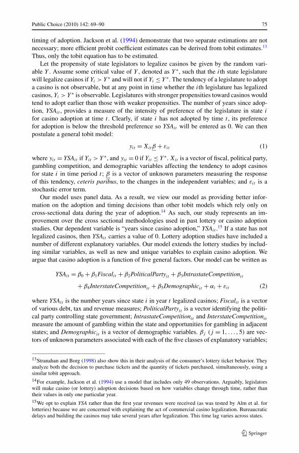
timing of adoption. Jackson et al. (1994) demonstrate that two separate estimations are notnecessary; more efficient probit coefficient estimates can be derived from tobit estimates.13

Thus, only the tobit equation has to be estimated.Let the propensity of state legislators to legalize casinos be given by the random vari-

able Y . Assume some critical value of Y , denoted as Y ∗, such that the ith state legislaturewill legalize casinos if Yi > Y ∗ and will not if Yi ≤ Y ∗. The tendency of a legislature to adopta casino is not observable, but at any point in time whether the ith legislature has legalizedcasinos, Yi > Y ∗ is observable. Legislatures with stronger propensities toward casinos wouldtend to adopt earlier than those with weaker propensities. The number of years since adop-tion, YSAit , provides a measure of the intensity of preference of the legislature in state i

for casino adoption at time t . Clearly, if state i has not adopted by time t , its preferencefor adoption is below the threshold preference so YSAit will be entered as 0. We can thenpostulate a general tobit model:

yit = Xitβ + εit (1)

where yit = YSAit if Yit > Y ∗, and yit = 0 if Yit ≤ Y ∗. Xit is a vector of fiscal, political party,gambling competition, and demographic variables affecting the tendency to adopt casinosfor state i in time period t ; β is a vector of unknown parameters measuring the responseof this tendency, ceteris paribus, to the changes in the independent variables; and εit is astochastic error term.

Our model uses panel data. As a result, we view our model as providing better infor-mation on the adoption and timing decisions than other tobit models which rely only oncross-sectional data during the year of adoption.14 As such, our study represents an im-provement over the cross sectional methodologies used in past lottery or casino adoptionstudies. Our dependent variable is “years since casino adoption,” YSAit .15 If a state has notlegalized casinos, then YSAit carries a value of 0. Lottery adoption studies have included anumber of different explanatory variables. Our model extends the lottery studies by includ-ing similar variables, as well as new and unique variables to explain casino adoption. Weargue that casino adoption is a function of five general factors. Our model can be written as

YSAit = β0 + β1Fiscalit + β2PoliticalPartyit + β3IntrastateCompetitionit

+ β4InterstateCompetitionit + β5Demographicit + αi + εit (2)

where YSAit is the number years since state i in year t legalized casinos; Fiscalit is a vectorof various debt, tax and revenue measures; PoliticalPartyit is a vector identifying the politi-cal party controlling state government; IntrastateCompetitionit and InterstateCompetitionit

measure the amount of gambling within the state and opportunities for gambling in adjacentstates; and Demographicit is a vector of demographic variables. βj (j = 1, . . . ,5) are vec-tors of unknown parameters associated with each of the five classes of explanatory variables;

13Stranahan and Borg (1998) also show this in their analysis of the consumer’s lottery ticket behavior. Theyanalyze both the decision to purchase tickets and the quantity of tickets purchased, simultaneously, using asimilar tobit approach.14For example, Jackson et al. (1994) use a model that includes only 49 observations. Arguably, legislatorswill make casino (or lottery) adoption decisions based on how variables change through time, rather thantheir values in only one particular year.15We opt to explain YSA rather than the first year revenues were received (as was tested by Alm et al. forlotteries) because we are concerned with explaining the act of commercial casino legalization. Bureaucraticdelays and building the casinos may take several years after legalization. This time lag varies across states.

76 Public Choice (2010) 142: 69–90

αi represents individual state-level random effects, allowing us to capture variation in anyunobserved state heterogeneity over time; and εit are the normally distributed disturbanceterms associated with the casino industry per se (in any state). These individual variables aredescribed in more detail below. We employ this random effects specification based on theresults of a likelihood ratio test which revealed the relative efficiency of the random effectsmodel as compared to both a fixed effects model (one including state level dummy variables)and a simple pooled tobit specification ignoring both fixed and random cross state effects.16

Considered in the context of our tobit model, a positive sign on a coefficient (i.e., positiveeffect) implies that increases in the variable cause the “years since casino adoption” (YSA) tobe larger. Hence, a positive coefficient increases the likelihood of adoption, and implies anearlier adoption of casinos relative to other states. A negative sign on a coefficient (a nega-tive effect) implies that a state is less likely to adopt casinos and, if it does adopt, it is likelyto adopt later, relative to other states.

3.2 Data

We have 800 observations: annual data from 1985 to 2000, for all 50 states. Table 2 lists thevariables in our model, along with brief definitions, data sources, and descriptive statistics.17

We are particularly interested in the fiscal and gambling competition variables because theyare the most common issues that arise in casino adoption debates.

3.2.1 Fiscal variables

The fiscal variables are meant to account for state specific fiscal conditions and institutionalconstraints that might push legislators toward casino legalization. Inclusion of these vari-ables follows earlier papers on gambling adoption, such as Alm et al. (1993). Our fiscalvariables include the log of short-term state debt (Debt-short term), the log of long-termstate debt (Debt-long term),18 a dummy variable to indicate whether a state has a tax andexpenditure limit (TEL, Tax/expend. limit),19 state tax revenue per capita (State revenue),and per capita federal government transfers to the state (Fed. transfers).

Fiscal pressure or stress may serve as a motivation for state governments to legalize casi-nos. There are a number of ways one can conceive of “fiscal stress”: taxpayers want moregovernment services, or they want lower taxes; increasing existing taxes is politically infea-sible; ever-increasing budget deficits; etc. Thus, these variables could indicate that politi-cians are reacting to fiscal pressure such as increasing budget deficits. Alternatively, theymay indicate that politicians, acting as an interest group, merely want to maximize revenueto expand the size and scope of government.

16Models using panel data typically include either fixed or random effects. In earlier specifications of ourmodel we incorporated state and/or regional dummies. However, these were not significant and did not ap-preciably affect the results associated with the basic variables in our model, so they were omitted. The like-lihood ratio test for random effect versus pooled time series tobit produces a χ2 = 658.7, rejecting the nullhypothesis that σα , the cross-state variance = 0. We are grateful to an anonymous referee for suggesting therandom effects tobit model.17As we are using panel data, it is unclear how useful descriptive statistics can be, but they are included forinterested readers.18We also tested per capita debt and found similar results.19There is a large variety of such rules, among which our variable does not distinguish. For a concise discus-sion of TELs, see http://www.ncsl.org/programs/fiscal/telsabout.htm.

Public Choice (2010) 142: 69–90 77

Table 2 Variable descriptions, descriptive statistics, and data sources

Variable Description Mean Std. Dev. Data source

Fiscal

Yrs. since adoption(dep. variable)

Number of years sincecasino legislation passed

2.21 9.069 Calculated by authors, withopening year data fromstate gamblingcommissions

Debt-long term Log of state govt. long termdebt

6.86 0.784 U.S. Census Bureau,Government Finance

Debt-short term Log of state govt. shortterm debt

0.35 2.003 U.S. Census Bureau,Government Finance

Tax/expend. limit State has tax andexpenditure limit, 1 = yes;0 = no

0.48 0.500 Book of the States

State revenue Real state govt. revenue percapita

8985.91 1019.17 Statistical Abstract of theU.S.

Fed. transfers Real intergovernmentaltransfers per capita

2353.91 2907.91 Statistical Abstract of theU.S.

Political party

Party of governor Party of governor,1 = Democrat; 0, otherwise

0.51 0.500 Book of the States

Dem.-unified govt. Democrat governor/legisl.majority = 1; 0, otherwise

0.24 0.428 Book of the States

Rep.-unified govt. Republican governor/legisl.majority = 1; 0, otherwise

0.43 0.495 Book of the States

Intrastate competition

Dog bets Greyhound racing bets percapita

11.43 22.438 Assoc. of RacingCommissioners Intl., Inc.

Horse bets Horse racing bets per capita 32.06 38.900 Assoc. of RacingCommissioners Intl., Inc.

Lottery sales Lottery ticket sales percapita

56.41 75.366 LaFleur’s 2001 WorldLottery Almanac, 9e

Indian casino sq ft Indian casino squarefootage per capita

0.02 0.061 Calculated by the authorswith data fromwww.casinocity.com andcalls to casinos

Interstate competition

River border State has a river on itsborder, 1 = yes, 0 = no

0.58 0.494 Calculated by the authors

Adj. state w/casino Percent of adjacent statesthat have casino(s)

0.14 0.174 Calculated by the authors

Adj state w/Indiancasino

Percent of adjacent statesthat have Indian casino(s)

0.28 0.263 Calculated by the authors

Square mileage State total area (squaremiles, excluding bodies ofwater)

70745.4 85176.5 U.S. Census Bureau,American Fact-Finder

Debt-short term and Debt-long term are thought to indicate whether the state is experi-encing fiscal stress or pressure. Long-term debt is usually associated with off-budget capitalexpenses, while short-term debt is usually an indication of a shortfall in revenues or a grow-

78 Public Choice (2010) 142: 69–90

Table 2 (Continued)

Variable Description Mean Std. Dev. Data source

Demographic

Baptists Percent of population thatare Baptists

12.31 13.526 New Book of AmericanRankings

Hotel employees Percent of state workersemployed by hotels

2.21 3.245 Bureau of EconomicAnalysis

Income Real per capita income 14506.75 2331.07 Bureau of EconomicAnalysis

Population density Population divided bysquare mileage

170.73 236.94 U.S. Census Bureau

Population over 65 Percent of population 65 orolder

12.54 2.066 U.S. Census Bureau

Poverty Percent of population belowpoverty line

13.95 4.124 U.S. Census Bureau

Unemployment State unemployment rate 5.57 1.763 Bureau of Labor Statistics

ing budget deficit. If state legislatures adopt casinos to collect additional tax revenue inorder to address these fiscal pressures, then we would expect the signs on Debt-short termand Debt-long term to be positive.

Tax and expenditure limits (TELs) indicate the ease with which state legislatures can ad-dress changes in fiscal conditions within the state. The existence of a Tax/expend. limit mightincrease the probability and timing of casino adoption as politicians attempt to circumventthese restrictions. State revenue measures the current revenue being collected by the stategovernment. As revenues decline we can expect that legislatures would be more inclinedto legalize casinos to address revenue shortfalls, ceteris paribus. Finally, Fed. transfers isthe amount of money received through inter-governmental transfers. If the amount of fundsfrom the federal government increases, we argue state legislatures would be less likely toadopt casinos, as they do not perceive as strong a need for additional tax revenue.

3.2.2 Political party variables

Proposals to legalize casino gambling always stir lively debate. Yet, it is unclear whetherone political party is consistently pro-casino and the other is anti-casino. The political partyvariables are included to examine whether casino legalization is more likely to occur whenone political party or the other holds power in state government. Party of governor is adummy variable with a value of 1 indicating the governor is a Democrat and 0 otherwise.Dem.-unified govt. is a dummy to indicate when the governor and legislative majority inthe state are Democratic, and Rep.-unified govt. indicates when the governor and legislativemajority are Republican.

Our purpose here is not to exhaustively explain why Democrats or Republicans vote forthe policies they do; there may be any number of explanations as to why one party or theother might support or oppose casinos. However, we believe the party variables may shedsome light on two political positions that are particularly relevant to casino legalization.The first is a “social liberal” effect. Democrats are typically seen as being more sociallyliberal, and may be more likely than Republicans to support gambling as an acceptableactivity. Some Republicans (i.e., the “religious right” or “Christian conservatives”) vocalizea strong moral opposition to gambling. To the extent that socially liberal values explain

Public Choice (2010) 142: 69–90 79

casino adoption, we would expect positive coefficients on Party of governor and Dem.-unified govt., and a negative coefficient on Rep.-unified govt.20

Alternatively, the political party variables may also reflect an “economic conservatism”effect. Republicans are often reputed to be more economically conservative than De-mocrats.21 If this is the case, Republicans may be more motivated to legalize casinos inorder to lower budget deficits, or as an alterative to raising income or property taxes in thestate. (This is similar to Furlong’s “political” effect.) If “economic conservatism” helps toexplain casino adoption, then we would expect Party of governor to be negative and Rep.-unified govt. to have a positive coefficient. Similarly, a negative coefficient on Dem.-unifiedmight be viewed as consistent with a lack of economic conservatism by Democrats.

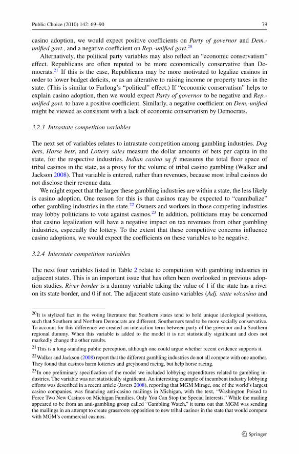
3.2.3 Intrastate competition variables

The next set of variables relates to intrastate competition among gambling industries. Dogbets, Horse bets, and Lottery sales measure the dollar amounts of bets per capita in thestate, for the respective industries. Indian casino sq ft measures the total floor space oftribal casinos in the state, as a proxy for the volume of tribal casino gambling (Walker andJackson 2008). That variable is entered, rather than revenues, because most tribal casinos donot disclose their revenue data.

We might expect that the larger these gambling industries are within a state, the less likelyis casino adoption. One reason for this is that casinos may be expected to “cannibalize”other gambling industries in the state.22 Owners and workers in those competing industriesmay lobby politicians to vote against casinos.23 In addition, politicians may be concernedthat casino legalization will have a negative impact on tax revenues from other gamblingindustries, especially the lottery. To the extent that these competitive concerns influencecasino adoptions, we would expect the coefficients on these variables to be negative.

3.2.4 Interstate competition variables

The next four variables listed in Table 2 relate to competition with gambling industries inadjacent states. This is an important issue that has often been overlooked in previous adop-tion studies. River border is a dummy variable taking the value of 1 if the state has a riveron its state border, and 0 if not. The adjacent state casino variables (Adj. state w/casino and

20It is stylized fact in the voting literature that Southern states tend to hold unique ideological positions,such that Southern and Northern Democrats are different; Southerners tend to be more socially conservative.To account for this difference we created an interaction term between party of the governor and a Southernregional dummy. When this variable is added to the model it is not statistically significant and does notmarkedly change the other results.21This is a long-standing public perception, although one could argue whether recent evidence supports it.22Walker and Jackson (2008) report that the different gambling industries do not all compete with one another.They found that casinos harm lotteries and greyhound racing, but help horse racing.23In one preliminary specification of the model we included lobbying expenditures related to gambling in-dustries. The variable was not statistically significant. An interesting example of incumbent industry lobbyingefforts was described in a recent article (Javers 2008), reporting that MGM Mirage, one of the world’s largestcasino companies, was financing anti-casino mailings in Michigan, with the text, “Washington Poised toForce Two New Casinos on Michigan Families. Only You Can Stop the Special Interests.” While the mailingappeared to be from an anti-gambling group called “Gambling Watch,” it turns out that MGM was sendingthe mailings in an attempt to create grassroots opposition to new tribal casinos in the state that would competewith MGM’s commercial casinos.

80 Public Choice (2010) 142: 69–90

Adj. state w/Indian casino) are the percentage of adjacent states that offer that type of casinogambling. These variables represent the degree of availability of casinos in nearby states.Finally, Square mileage is the total land area of the state, which may affect the likelihoodthat residents will travel to adjacent-state casinos, and conversely, how many tourists thestate is likely to attract from adjacent states.

There are at least three reasons why having a river on the state’s border might makecasino adoption more likely. First, and most importantly, allowing riverboat casinos onrivers/state borders may represent an aggressive attempt to attract tourists (and tax revenues)from neighboring states. Second, one could argue that river borders have a political signifi-cance. Voters or politicians with “moral” objections to casinos on state land may be appeasedif casinos are allowed only on riverboats, since technically the gambling would not be oc-curring within the state. Third, riverboat casinos could be promoted on historical grounds.If such boats were legal at an earlier time, perhaps the argument for legalizing casinos canbe made stronger by citing an historical precedent. As most of the early-adopting states (IA,IL, IN, MS, MO, and LA) border the Mississippi River, we expect this variable to have apositive coefficient.

If a nontrivial portion of a state’s population travels out-of-state in order to visit casinos,politicians can make an argument that casinos should be adopted within the state to keepits citizens—and tax money—within the state. Furlong (1998) calls this the “competitiverationale” for legalizing casinos; it is also called “defensive legalization” in the gamblingliterature. A current example of this argument can be seen in Massachusetts, whose resi-dents spent an estimated $876 million at Connecticut casinos in 2006 (Barrow 2007). Thegovernor is seeking to legalize casinos in Massachusetts, in part, to allow residents to gambleat casinos within the state.

Lottery adoption studies have typically used rather blunt variables for measuring inter-state competition, if they consider it at all. For example, Alm et al. (1993) use a dummyvariable to indicate whether any neighboring state has a lottery.24 A variable that is moresensitive to the extent to which state residents have options in neighboring states would bepreferred to a simple dummy. Therefore, following Davis et al. (1992) and Walker and Jack-son (2008), our variables measure the percentage of adjacent states with commercial casinosor Indian casinos.25 To the extent that politicians are motivated to adopt casinos in order tokeep tax revenues in-state (defensive legalization), we would expect the coefficients on Adj.state w/casino and Adj. state w/Indian casino to be positive.

The last variable in the interstate competition category is the size of the state, Squaremileage. We view the size of the state as potentially affecting the extent to which consumerswithin the state are likely to travel outside to neighboring states in order to gamble. Thelarger the state, the less likely a person may be to travel out-of-state, simply because thelarger the state, the longer and costlier the drive is likely to be.26 The size of the state could

24Neither Jackson et al. (1994) nor Filer et al. (1988) include a variable to account for neighboring statelotteries.25Walker and Jackson (2008) explain that this type of measure is preferable to a dummy because it is moresensitive to the degree to which residents have access to casino gambling in neighboring states. Using the sumof adjacent states’ revenues would be problematic because larger totals could result from larger populations,more tourism, or a combination of the two. A per capita measure of adjacent total revenues is similarlyproblematic, because higher total per capita revenues in adjacent states may reflect more gambling, moreneighboring states, or fewer residents in those states. Overall, these measures are less effective than thepercentage of adjacent states at measuring simple gambling availability in neighboring states.26This effect obviously would depend on a number of factors, including the distribution of population relativeto the state’s border. But consider two states, one large and one small, and each having identical uniformly

Public Choice (2010) 142: 69–90 81

have an analogous effect on neighboring states’ tourists. The larger a particular state, theless likely it is that people from neighboring states will visit it, ceteris paribus.

3.2.5 Demographic variables

Finally, we turn to the demographic variables in the model. These variables can be seenas gauging constituents’ characteristics, but they also could be indicators for the casinoindustry as to the extent to which the state’s residents are likely to be consumers of itsproduct. Previous papers have included a variable to represent potential religious oppositionto gambling.27 We include as a variable the percentage of the state’s population that is Baptist(Baptists), as this group is an organized, well-known opponent of legalized gambling. Wewould expect Baptists to have a negative coefficient.

Clearly, legislators can garner significant rents from the voting public if they can designrevenue strategies to induce non-residents to pay part of the state’s tax bill. One such strategyis to attract out-of-state tourist and then tax them, thereby “exporting” part of the state’stax bill to the tourists’ states of origin. Popular examples of this include accommodationstaxes and taxes on rental cars, which are largely paid by tourists. We include a variable thatmeasures the percentage of the state’s total employment that works in the hotel industry(Hotel employees) as a proxy for the tourism industry. The larger this number, the larger thestate’s tourism sector, ceteris paribus. We expect this variable to have a positive effect oncasino adoption and timing, as this would be consistent with efforts to expand tourism andtax exporting.

In states with higher income per capita, we expect consumers to spend more money onleisure activities. We include per capita income in the model (Income), with the expectationthat it will carry a positive sign. This would suggest that casino gambling is a normal good,or perhaps that the residents prefer taxes on casinos to income, sales, property, or otheruniversally applied taxes.

We include the state’s population density as an explanatory variable (Population density).Casinos may be more likely to be built if there are significant population centers that couldsupport such businesses. If the industry requires a minimum threshold of people to surviveand if the state’s residents are the primary consumers of casino services, then we mightexpect this variable to have a positive effect on adoption.

The proportion of the state’s population age 65 or over is included as a variable (Popu-lation over 65). Casino opponents have argued that older people are taken advantage of bycasinos. On the other hand, retirees may favor more entertainment choices and have loweropportunity costs of time. Also, since the older population is an influential block of voters,we include it in the model. Given that casinos are often popular with the older population,due perhaps to their lower opportunity cost of time, we could expect this variable to have apositive effect on casino adoption.

One of the major concerns over gambling is whether poor people over-consume suchservices. The regressivity of the lottery “tax” has received enormous attention in the litera-

distributed population with transportation equally difficult in all directions. Now randomly pick a personfrom each state; the person in the small state is more likely to reside closer to a border than the person pickedfrom the large state, ceteris paribus. It follows that the person in the small state is more likely to travel to aneighboring state, ceteris paribus, since the cost of doing so would be lower.27For example, Alm et al. (1993) use the percentage of population that is Catholic and Jackson et al. (1994)and Elliott and Navin (2002) use Baptists as variables to explain lottery adoption.

82 Public Choice (2010) 142: 69–90

ture.28 If taxes on casino gambling represent a similarly regressive tax, then we may expectthe proportion of poor people in the state (Poverty) to have a negative impact on casinoadoption, to the extent politicians and voters share a concern for the poor. Of course, thefact that most states have lotteries suggests that politicians have other concerns greater thangambling tax regressivity. Our last demographic variable is the unemployment rate in thestate (Unemployment). We might expect a state to be more likely to adopt casinos if they areexpected to stimulate employment and economic growth. This motivation to adopt may begreater in states with slower economies and more unemployment.

4 Results

We present results of the random effects model in Table 3. The coefficients shown representthe decomposition of the tobit coefficient, as utilized by Jackson et al. (1994). Specifically,the tobit coefficient represents the “timing” effect, while the “probability of adoption” effectis shown in the implied probit coefficient.29 Note that the probability and timing effectsare jointly estimated, so that the z-statistics on the variables shown in Table 3 measure thesignificance of both the tobit regression coefficient and the implied probit coefficient foreach variable.

4.1 Random effects tobit model

As indicated in Table 3, two of the five fiscal variables, Debt-long term and Tax/expend.limit, are statistically significant at the 1% level. Debt-long term is positive and significantsuggesting that states with higher long term debt are more likely to adopt casinos, and todo it sooner. Tax/expend. limit is also positive, which suggests that legislatures perceive taxrevenues from casino gambling as a way to increase revenues and spending where they mayotherwise face constraints. While our results provide some evidence that fiscal variablesinfluence the decision to adopt casinos, these results are largely consistent with those byFurlong (1998), Alm et al. (1993), and Jackson et al. (1994), who found little support forfiscal pressure as a motivation for adopting casinos or lotteries.30

Among the political party variables, Rep.-unified govt. and Party of governor are sta-tistically significant (1% level). Dem.-unified govt. is insignificant. The combination of apositive coefficient on Rep-unified govt. and negative coefficient on Party of governor aremost consistent with our “economic conservatism” motivation for adoption. These resultsmay indicate that the “social liberal” motivation discussed earlier may not be as importantas fiscal motivations, with respect to casino adoption.

28See Clotfelter and Cook (1991), Hansen (1995), Miyazaki et al. (1998), and Stranahan and Borg (1998)for examples. Even when the expenditure of lottery revenue is considered, for example, to subsidize collegeeducation, many lotteries remain regressive, as benefits are often paid disproportionately to higher-incomerecipients (Rubensetin and Scafidi 2002).29The probability effect is the marginal effect from the probit coefficient. It is calculated, for a given variable(say the j th), as the estimated tobit coefficient (βj ) divided by the estimated standard error of the regression

(σ), calculated as the square root of the overall variance (σ 2e ) and the panel-level variance (σ 2

α ), where σ =√σ 2e + σ 2

α . This implied probit coefficient is multiplied by the ordinate of the standard normal distribution,evaluated at the predicted z value of the implied probit equation (f (z̄)); that is, (βj /σ ) ∗ f (z̄).30The exception, as noted previously, is Alm et al. (1993), who found that fiscal stress did explain early (butnot later) lottery adoptions.

Public Choice (2010) 142: 69–90 83

Table 3 Random effects tobit on casino adoption (Dependent variable: Yrs. since adoption)

Variable Timing effect Probability effecta z-stat.

(Tobit) (Probit)

Fiscal

Debt-long term 1.604 0.020 2.66∗∗∗Debt-short term −0.022 −0.0003 −0.37

Tax/expend. limit 3.076 0.039 7.64∗∗∗State revenue −8.5e−5 −1.1e−6 −0.70

Fed. transfers 0.0004 5.1e−6 0.76

Political Party

Party of governor −0.898 −0.012 −2.52∗∗Dem.-unified govt. 0.556 0.007 1.17

Rep.-unified govt. 0.784 0.010 2.53∗∗∗Intra-state competition

Dog bets −0.041 −0.001 −2.85∗∗∗Horse bets 0.012 0.0002 4.13∗∗∗Lottery sales 0.006 8.0e−5 3.25∗∗∗Indian casino sq ft −18.50 −0.236 −5.15∗∗∗Inter-state competition

River border 5.340 0.068 5.29∗∗∗Adj. state w/casino 0.923 0.012 0.99

Adj. state w/Indian casino 8.682 0.111 8.43∗∗∗Square mileage −3.1e−7 −3.9e−9 −0.05

Demographic

Baptists 0.211 0.003 6.68∗∗∗Hotel employees 1.724 0.022 42.96∗∗∗Income 0.001 1.6e−5 7.80∗∗∗Population density −0.003 −3.3e−5 −2.25∗∗Population over 65 −0.369 −0.005 −1.88∗Poverty −0.657 −0.008 −6.59∗∗∗Unemployment −0.209 −0.003 −1.91∗Constant −26.02 −0.332 −4.61∗∗∗

N = 800; σe = 0.817; σα = 31.23; χ2 = 29694.6

Notes: *indicates significance at the 0.10 level, **at the 0.05 level, and ***at the 0.01 level. σe is the overall

standard error of the estimate and σα is the panel level standard error. χ2 tests the joint significance of allexplanatory variablesaThe probit coefficient is calculated as described in footnote 29

We next turn to the intrastate competition variables. All of the tested variables on in-state gambling are significant at standard levels. However, the results are mixed. Dog betsand Indian casino sq ft are consistent with the in-state competition effect discussed earlier.However, this result is somewhat surprising; we would have thought that if the state alreadyhas Indian casinos, politicians would be interested in capturing some of the potential tax rev-enues through commercial casinos. Perhaps our result simply reflects reluctance by votersto increase the number of casinos in a state, once Indian casinos are already present. Alter-

84 Public Choice (2010) 142: 69–90

natively, it is conceivable that companies managing tribal casinos lobby to prevent furthercompetition, or to ensure that tribal-state compacts prevent further competition.31

Both Horse bets and Lottery sales have a positive and significant impact on casino adop-tion.32 These results may reflect a general attitude toward gambling, rather than a large con-cern over inter-industry competition. That is, if the state’s citizens or legislators are alreadyamenable to gambling—or if they simply appreciate the tax revenues it brings—casino adop-tion is more likely. One may find, for example, that the standard arguments against gamblingare considered to be inconsequential if the state already has legalized gambling in some formand is satisfied with it.

Next we consider the interstate variables, which are generally very supportive of the in-terstate competition motivation for casino legalization. The River border variable is positiveand significant at the 1% level. States with rivers bordering them may find it relatively easyto adopt casinos because of loopholes regarding gambling on water. This result may alsoreflect the historical or moral issues discussed earlier. Most importantly, the positive rivereffect is consistent with the argument that states attempt to export taxes by attracting tourismfrom neighboring states.

The results on the adjacent state casino variables also support interstate competition asa motivation for casino adoption. We find Adj. state w/Indian casino is significant at the1% level, indicating that states with a larger proportion of neighboring Indian casino statesare more likely to adopt commercial casinos. The coefficient on Adj. state w/casino whilepositive, is insignificant. This insignificance may simply be due to the fact that still relativelyfew states have legal commercial casinos.

Finally Square mileage is negative and insignificant, indicating that state size does notaffect casino adoptions. The sign itself implies that larger states may be less likely to drawborder-crossing tourists due to their size, and they are less likely to have their own residentstravel to adjacent states with casinos. For this reason there is less motivation, based oninterstate competition, to legalize casinos.

The results of our demographic variables are, in some cases, unexpected. However, weview these variables as being secondary in importance for our study; our main interestsare the fiscal and gambling competition variables. We find that Baptists has a significantand positive (1% level) effect on casino adoption. Clearly, this result is contrary to ourexpectations. However, since Mississippi and Louisiana were among the first states to adoptcasinos, perhaps Baptists is picking up a “Southern” effect in our model.33

Population density is negative and significant (1% level) in the model. This result mayindicate that adopting legislatures view the potential casino market to arise from out-of-state

31An example of this would be the compact in Connecticut, where the state receives 25% of slot revenuesfrom the tribal casinos in exchange for a guarantee that additional casinos will not be permitted in the state.As noted previously, lobbying expenditures related to gambling industries was not statistically significant ina preliminary specification of the model.32See footnote 22. The negative sign of Dog bets and the positive sign on Horse bets is consistent with thefindings of Walker and Jackson (2008).33Another possibility is raised by the Mississippi case. Prior to casinos being legalized there, a proposalfor a state-run lottery was defeated soundly in a referendum against which Baptists lobbied heavily. Casinogambling subsequently passed in Mississippi with virtually no public debate, and the legislature did not putit to a popular vote. Casinos were sold as a way of funding K-12 education, but the promise was arguablynot fulfilled. This raises an important issue: To what extent does casino legalization depend on its revenuesbeing earmarked for particularly “good” purposes? Only three states with commercial casinos (Michigan,Missouri, and Pennsylvania) advertise the fact that casino tax revenues are earmarked. This would be animportant issue for future research: What attributes of casino legislation affect passage? However, this issueis beyond the scope of this paper.

Public Choice (2010) 142: 69–90 85

tourists, rather than local residents. Clearly, most casino markets have developed outside ofurban settings; this is consistent with our findings. As we expected, Hotel employees is sig-nificant and positive. This gives further support to the argument that casinos are adoptedwith the intent of attracting tourism and/or exporting taxes. Income is also found to have apositive impact on adoption. This suggests that states with higher-income citizens may pre-fer having additional leisure options and/or prefer having alternatives to higher income orproperty taxes; it may also suggest that gambling is a normal good, or simply that individ-uals with relatively high incomes support shifting the tax burden to casino customers. ThePopulation over 65 in a state has a negative and significant impact on the likelihood or timingof casino adoption. As expected, this group has an effect on the outcome of most politicalissues, including the adoption of casinos. States with relatively larger elderly populationsare not as likely to legalize casinos. As anecdotal support for this finding, consider Florida,which has by far the largest proportion of citizens over 65 years old. Casino legalizationproposals have repeatedly been defeated there. This finding conflicts with our expectations,which were that individuals with more spare time would support additional entertainmentoptions. Perhaps casinos are not needed in Florida, as individuals who wish to gamble haveready access to cruise ships with casinos.

The more Poverty, the less likely is casino adoption. This result is consistent with thetax-shifting motivation from above, and with the argument that politicians (and voters) tendto shy away from perceived regressive forms of taxation. (Perhaps the regressivity issue hasbecome more important as the effects of the lottery “tax” have become better understood.)Finally, Unemployment has a statistically significant and negative effect on adoption. Con-trary to the public debates over casino gambling, our results suggest that politicians do not,in fact, pursue legalized casinos as a means of dealing with high unemployment, or moregenerally, bad economic conditions.

4.2 Random effects tobit model with simultaneity

One can argue that states adopt casinos, as least in part, to have a revenue source in orderto finance long-term debt. This argument suggests that endogeneity might exist betweenYSA and Debt-long term. To test for this simultaneous relationship we use a version of theHausman omitted variable test. We regress Debt-long term on the same set of explanatoryvariables as noted in (2), along with two additional variables (real capital outlays per capita,and a dummy for a balanced budget rule) to identify the implied system of equations. Bothof these new variables may affect long-term debt, but should not be predictors of casinoadoption.34 We estimate a random effects tobit model to test for simultaneity by includingthe residuals from the long term debt equation, along with Debt-long term in the YSA model.Both Debt-long term and the residuals of Debt-long term prove to be statistically significant,suggesting that endogeneity does exist between YSA and Debt-long term.35

While we do not know the direction of causality between adoption and long term debt,the existence of simultaneity is consistent with the legislator-as-interest-group theory. Wehave argued earlier that long term debt should positively affect casino adoption, but thepossibility that adoption also affects long term debt suggests that legislatures may be lookingfor revenue sources to provide largess in the form of capital expenditures, or other spending

34We tested balanced budget rules in a preliminary model of casino adoption and it was insignificant.35See Gujarati (2003: 754–755) or Pindyck and Rubinfeld (1991: 303–305). For an analysis involving morethan two endogenous variables, see Kennedy (2003: 197–198). It is worth noting that the previous literatureon lottery adoption does not address the issue of a simultaneous system.

86 Public Choice (2010) 142: 69–90

Table 4 Random effects tobit on casino adoption: corrected for simultaneity (Dependent variable: Yrs. sinceadoption)

Variable Timing effect Probability effecta z-stat.

(Tobit) (Probit)

Fiscal

Debt-long term 2.141 0.028 2.15∗∗Debt-short term −0.077 −0.001 −1.26

Tax/expend. limit 3.222 0.042 9.45∗∗∗State revenue −0.0002 −2.79e−6 −1.9∗Fed. transfers 0.0008 1.06e−5 1.85∗Political Party

Party of governor −1.484 −0.019 −3.65∗∗∗Dem.-unified govt. 1.333 0.017 2.71∗∗∗Rep.-unified govt. 1.119 0.015 3.34∗∗∗Intra-state competition

Dog bets −0.030 −0.0004 −2.27∗∗Horse bets 0.003 4.45e−5 0.73

Lottery sales 0.002 2.43e−5 0.78

Indian casino sq ft −21.49 −0.279 −5.61∗∗∗Inter-state competition

River border 5.291 0.069 7.46∗∗∗Adj. state w/casino 1.866 0.024 1.97∗∗Adj. state w/Indian casino 8.90 0.115 7.84∗∗∗Square mileage −5.7e−5 −7.3e−7 −6.8∗∗∗Demographic

Baptists 0.168 0.002 4.79∗∗∗Hotel employees 1.863 0.024 59.76∗∗∗Income 0.001 1.66e−5 8.85∗∗∗Population density −0.006 −8.3e−5 −5.59∗∗∗Population over 65 −0.368 −0.005 −1.79∗Poverty −0.069 −0.009 −6.83∗∗∗Unemployment −0.272 −0.004 −2.53∗∗∗Constant −23.75 −0.308 −3.36∗∗∗

N = 800; σe = 0.829; σα = 30.71; χ2 = 29601.24

Notes: *indicates significance at the 0.10 level, **at the 0.05 level, and ***at the 0.01 level. σe is the overall

standard error of the estimate and σα is the panel level standard error. χ2 tests the joint significance of allexplanatory variablesaThe probit coefficient is calculated as described in footnote 29

that requires long term debt. The random effects tobit model corrected for endogeneity usesthe predicted value of long term debt (Debt-long term*) as an instrument for Debt-long term.The results of the model corrected for endogeneity are shown in Table 4.

Overall, the results of this model are consistent with the initial random effects model.None of the signs on the explanatory variables change, and the levels of significance gener-

Public Choice (2010) 142: 69–90 87

ally improve. Our discussion of these results will focus on the few differences between thetwo sets of results.

The fiscal variables perform better when (2) is corrected for endogeneity. Debt-longterm* and Tax/expend. limit continue to be statistically significant. State revenue is nega-tive and becomes significant on the probability and timing of adoption, as anticipated. Thisreinforces the short-sighted time horizon view of political decision making. Since revenuescorrespond to current spending ability, legislators are less likely to adopt casinos if tax rev-enues increase. Fed. transfers are positive and significant (10% level). Receiving greateramounts of inter-governmental transfers encourages states to adopt casinos.

Overall, our fiscal variables are mixed with regards to fiscal pressure being a motiva-tion for adoption. Debt-long term* suggests that legislatures are more likely to adopt andadopt sooner when long term debt increases, but Debt-short term is insignificant. The posi-tive signs on Tax/expend. limit and Fed. transfers both suggest that legislators are adoptingcasinos as additional sources of revenue, but not because of fiscal stress or pressure. Thefiscal variables seem to matter only when politicians have either already incurred the debt,when they are looking for ways to raise revenue outside of the normal tax structure, or whenrevenues from the federal government are increasing. These results appear to support the“legislature-as-interest-group” theory.

The only change in the political variables is that Dem.-unified is now significant (1%level). A Democratic-controlled government, similar to a Republican-controlled govern-ment, is more likely to adopt casinos and adopt them sooner than divided governments.This combination of political variable results (Dem.-unified and Rep.-unified positive, withParty of governor negative) is inconsistent with both our “social liberal” and “economicconservative” hypotheses introduced earlier. Perhaps the best explanation of our politicalvariable results is akin to that offered by Jackson et al. (1994: 252–253). In the context oflottery adoption, they suggest that legislative majorities may be able to pass legislation morequickly because less negotiation, logrolling, and fewer revisions to legislation may be nec-essary when the other party has little power. A similar explanation may apply to our results,where political party appears not to affect casino adoption, but having a unified governmentdoes have a significantly positive impact on casino adoption and timing.

Intrastate competition variables represent the greatest change between the two models.Horse bets and Lottery sales are still positive, but no longer are statistically significant. Thisresult is more consistent with our initial expectations that the existence of these gamingindustries might discourage adoption, or in this case have no effect. More specifically, thechange in significance suggests that Horse bets and Lottery sales affect YSA through anindirect route that is transmitted through Debt-long term*.36

The results on the adjacent state competition variables also improve and further supportinterstate competition as a motivation for casino adoption. We find that states with a larger

36Both Horse bets and Lottery sales are positive and significant (1% level) in the regression equation used

to estimate Debt-long term*. These results might imply that the presence of these gambling outlets increaseslong-term debt, which would also be consistent with the legislator-as-interest-group hypothesis. The “indi-rectness” of the effect of these variables on YSA can be seen by comparing their results in Table 3 with thosein Table 4. In the first case, their respective effects on YSA are statistically significant but ceteris paribus, i.e.,holding constant the long term debt effects on YSA. In Table 4, however, the significant positive effects ofHorse bets and Lottery sales on long term debt have been incorporated in the instrument Debt-long term*,so that these variables’ ceteris paribus effects on YSA are now insignificant. Thus, it appears that, rather thanacting independently, Horse bets and Lottery sales increase Debt-long term which in turn increases the prob-ability of casino adoption, and induces adopting states to adopt earlier. One explanation for this relationshipis that politicians may commit to new capital projects once they have obtained a new source of state revenuesthat they expect to provide a long-run stream of revenues.

88 Public Choice (2010) 142: 69–90

proportion of neighboring Indian and/or commercial casino states are more likely to adoptcasinos themselves. Adj. state w/Indian casino and Adj. state w/casino are significant atthe 1% and 5% level, respectively. In addition, Square mileage while still negative is nowsignificant (1% level), which means that larger states may be less likely to draw border-crossing tourists and to see their own residents travel to adjacent states with casinos. For thisreason there is less motivation to legalize casinos. This result meets our a priori expectationsand is further support for the interstate competition argument for casino adoption.

4.3 Summary

Accounting for both random effects across states and the issue of simultaneity improvesour econometric analysis.37 The evidence supporting fiscal stress as a motivation to legalizecasinos is mixed. The interstate competition motivation for casino legalization improveswhen we account for simultaneity and this is our strongest group of variables in the model.Our results suggest that any concerns over intrastate competition tend to be outweighed byother considerations, perhaps the prospect of additional or alternative tax revenues, or thepotential for exporting taxes and increased tourism.

5 Conclusion

The present study illuminates and expands the empirical analysis of gambling adoption. Weuse a random effects tobit model with panel data for the 50 states from 1985 to 2000. Our ex-planatory variables include fiscal, political party, intra- and interstate gambling competition,and demographic characteristics.

Media reports typically suggest that tax revenues are the primary motivation for legal-izing casinos, and this is reflected in public discourse over casinos. Our results find somesupport of this notion. We find evidence that casinos are adopted as a means of reducingfiscal stress with regards to long term debt and current state revenue, but not with regard toshort tem debt. The signs and significance on these variables are generally consistent withAlm et al. (1993).

The variables Debt-short term, Tax/expend. limit, and State revenue all support the theoryof state legislatures as an interest group. We also find compelling evidence to suggest thatstates legalize casinos as a means of attracting tourism and of keeping citizens who wishto gamble in-state. This is consistent with the goal of increasing intrastate tax revenues andexporting some taxes to other states. These findings also support the Jackson et al. (1994)and Filer et al. (1988) theory of the legislature as an interest group.

Our study can be viewed as an extension of the lottery adoption literature to a new in-dustry. We are aware of only one other empirical analysis of casino adoptions in the UnitedStates (Furlong 1998). Our study expands on and enhances Furlong’s limited study, as wetest many more variables and use more recent data. In addition, ours is the only study ongambling that suggests that a simultaneous relationship exists between long term debt andlegalization of gambling. Although our results provide interesting information on a number

37We attempted a number of alternative specifications. Other variables we tested included: (i) whether thestate approves casinos by referendum or voter initiative; (ii) a dummy to account for the 1988 IGRA; (iii) stateand regional dummies; (iv) balanced budget rules, and (v) Southern Democrat, an interaction term betweenParty of governor and a Southern regional dummy. None of these variables proved to be significant, nor didthey markedly affect our other results.

Public Choice (2010) 142: 69–90 89

of variables, there are clearly still other interesting questions yet to be resolved. For exam-ple, why have more states not already adopted casinos? After all, most state governmentshave given their implicit approval to gambling, generally, by sponsoring lotteries. Over halfof the states already have tribal casinos. Why not allow commercial casinos and generateeven more tax revenues? Perhaps politicians and voters are cognizant of the potential thatcasinos compete with lotteries and they are not confident about the net effects of casinoson tax receipts. Maybe vocal anti-casino grassroots organizations have been particularly ef-fective in convincing voters to oppose the expansion of casinos. Perhaps there are concernsabout the potential social harms that may accompany casino gambling. Or maybe citizenshave NIMBY (“not in my back yard”) concerns about casinos that do not apply to lotteries.All of these issues represent opportunities for future economic research on the commercialcasino industry in the United States.

References

Alm, J., McKee, M., & Skidmore, M. (1993). Fiscal pressure, tax competition, and the introduction of statelotteries. National Tax Journal, 46, 463–476.

American Gaming Association (2008). State of the states: the AGA survey of casino entertainment. Availableonline at http://www.americangaming.org. Accessed June 1, 2008.

Barrow, C. (2007). New England casino gaming update, 2007. Dartmouth: Center for Policy Analysis, Uni-versity of Massachusetts.

Berry, F., & Berry, W. (1990). State lottery adoptions as policy innovations: an event history analysis. Amer-ican Political Science Review, 84(2), 395–415.

Bluestein, G. (2009). States bet on gambling. Charleston Post and Courier (26 Jan.).Borg, M., Mason, P., & Shapiro, S. (1991). The economic consequences of state lotteries. New York: Praeger.Caudill, S., Ford, J., Mixon, F., & Peng, T. (1995). A discrete-time hazard model of lottery adoption. Applied

Economics, 21, 555–561.Clotfelter, C., & Cook, P. (1991). Selling hope: state lotteries in America. Cambridge: Harvard University

Press.Coughlin, C., Garrett, T., & Hernández-Murillo, R. (2006). The geography, economics, and politics of lottery

adoption. Federal Reserve Bank of St. Louis Review (May/June), 165–180.Davis, R., Filer, J., & Moak, D. (1992). The lottery as an alternative source of state revenue. Atlantic Economic

Journal, 20(2), 1–10.Elliott, D., & Navin, J. (2002). Has riverboat gambling reduced state lottery revenue? Public Finance Review,

30(3), 235–247.Erekson, O., Platt, G., Whistler, C., & Ziegert, A. (1999). Factors influencing the adoption of state lotteries.

Applied Economics, 31, 875–884.Filer, J., Moak, D., & Uze, B. (1988). Why some states adopt lotteries and others don’t. Public Finance

Quarterly, 16(3), 259–283.Furlong, E. (1998). A logistic regression model explaining recent state casino gaming adoptions. Policy Stud-

ies Journal, 26(3), 371–383.Garrett, T. (2001). The Leviathan lottery? Testing the revenue maximization objective of state lotteries as

evidence for Leviathan. Public Choice, 109, 101–117.Giacopassi, D., Nichols, M., & Stitt, B. (2006). Voting for a lottery. Public Finance Review, 34, 80–100.Glickman, M., & Painter, G. (2004). Do tax and expenditure limits lead to state lotteries? Evidence from the

United States: 1970–1992. Public Finance Review, 32, 36–64.Gujarati, D. (2003). Basic econometrics (4 edn.). New York: McGraw-Hill.Hansen, A. (1995). The tax incidence of the Colorado state lottery instant game. Public Finance Quarterly,

23, 385–398.Jackson, J., Saurman, D., & Shughart, W. (1994). Instant winners: legal change in transition and the diffusion

of state lotteries. Public Choice, 80, 245–263.Javers, E. (2008). MGM Mirage’s hidden card. Business Week (28 Feb.). Available online at

http://www.businessweek.com.Kennedy, P. (2003). A guide to econometrics (5 edn.). Cambridge: The MIT Press.Light, S., & Rand, K. (2005). Indian gaming & tribal sovereignty: the casino compromise. Lawrence: Uni-

versity Press of Kansas.

90 Public Choice (2010) 142: 69–90

Mixon, F., Caudill, S., Ford, J., & Peng, T. (1997). The rise (or fall) of lottery adoption within the logic ofcollective action: some empirical evidence. Journal of Economics and Finance, 21, 43–49.

Miyazaki, A., Hansen, A., & Sprott, D. (1998). A longitudinal analysis of income-based tax regressivity ofstate-sponsored lotteries. Journal of Public Policy & Marketing, 17, 161–172.

National Indian Gaming Commission (2008). NIGC announces 2007 Indian gaming revenues. Press release.Washington, DC. Available online at http://www.nigc.gov/ReadingRoom/PressReleases/.

Pindyck, R., & Rubinfeld, D. (1991). Econometric models and econometric forecasts (3 edn.). New York:McGraw-Hill.

Richburg, K. (2008). Governors seek remedies for shortfalls. Washington Post (13 Jan.).Rubensetin, R., & Scafidi, B. (2002). Who pays and who benefits? Examining the distributional consequences

of the Georgia Lottery for Education. National Tax Journal, 55(2), 223–238.Sirakaya, E., Dursun, D., & Hwan-Suk, C. (2005). Forecasting gaming referenda. Annals of Tourism Re-

search, 32(1), 127–149.Stranahan, H., & Borg, M. (1998). Separating the decisions of lottery expenditures and participation: a trun-

cated tobit approach. Public Finance Review, 26(2), 99–117.von Herrmann, D. (2002). The big gamble: the politics of lottery and casino expansion. Westport: Praeger.Walker, D. (2007). The economics of casino gambling. New York: Springer.Walker, D., & Jackson, J. (2008). Do U.S. gambling industries cannibalize each other? Public Finance Re-

view, 36(3), 308–333.