Determinants of Banks’ Liquidity: a French Perspective on Interactions

between Market and Regulatory Requirements

Olivier de Bandt1, Sandrine Lecarpentier2 and Cyril Pouvelle3

September 2020, WP 782

ABSTRACT

The paper investigates the impact of solvency and liquidity regulation on banks' balance sheet structure. The Covid-19 pandemics shows that periods of sharp increase in risk aversion often result in liquidity strains for banks due to the volatility of long-term funding markets. According to a simple portfolio allocation model banks’ liquidity increases when the regulatory constraint is binding. We provide evidence, using the “liquidity coefficient” implemented in France ahead of Basel III's Liquidity Coverage Ratio, of a positive effect of the solvency ratio on the liquidity coefficient. We also show that in times of crisis, measured by financial variables, French banks actually decreased the liquidity coefficient, with the transmission channel materialising mainly on the liability side.

Keywords: Bank Capital Regulation, Bank Liquidity Regulation, Basel III, Stress Tests

JEL classification: G28, G21

1 Economics and International Cooperation dept., olivier.debandt@banque-france.fr 2 Prudential Supervision and Resolution Authority and Paris-Nanterre University, EconomiX, CNRS, sandrine.lecarpentier@acpr.banque-france.fr 3 Prudential Supervision and Resolution Authority, cyril.pouvelle@acpr.banque-france.fr This work has benefited from insightful comments by participants in the ACPR research seminar and the 2019 EBA Policy Research Workshop. We are particularly grateful to Sylvain Benoit, Philippe Billard, Laurent Clerc, Christophe Hurlin, Catherine Lubochinsky, Valérie Mignon, Carmelo Salleo and Laura Valderrama who provided precious feedbacks at various stages of the project.

Working Papers reflect the opinions of the authors and do not necessarily express the views of the Banque de France. This document is available on publications.banque-france.fr/en

Banque de France WP #782 ii

NON-TECHNICAL SUMMARY

Capital and liquidity requirements present many interactions. While banks' capital regulation has been amply analysed in the literature, the estimation of banks' liquidity is still in its infancy. This can be explained by the fact that until recently there had not been any internationally harmonised liquidity ratio. The Covid-19 pandemics shows that periods of sharp increase in risk aversion often result in liquidity strains for banks due to the volatility of long-term funding markets. The latter react differently depending on the diversity of their funding sources and their risk profile. The first line of defence in those situations consists in using liquidity buffers to cope with cash outflows. But banks might also increase their liquidity buffers if they anticipate a long-lasting crisis and want to mitigate liquidity risks in the future. Finally, the central bank can also provide a form of insurance against systemic liquidity risks by providing unlimited amount of cash against collateral. During a crisis, due to interactions between funding and market liquidity, as well as regulatory constraints, one may wonder whether banks may increase or decrease liquidity. Banks’ liquidity may increase when the regulatory constraint is binding, as banks hoard extra liquidity, while they do not if the regulatory constraint is not binding. This study aims at estimating the determinants of banks' liquidity ratios, taking into account the interactions between solvency and liquidity as well as between market liquidity and funding liquidity risks. To that end, we estimate a system of simultaneous equations. We provide evidence, using the “liquidity coefficient” implemented in France ahead of Basel III's Liquidity Coverage Ratio, of a positive effect of the solvency ratio on the liquidity coefficient. Our results on a panel of French banks show that a higher level of solvency enables the liquidity ratio to improve due to balance sheet adjustments. By contrast, we do not find evidence that solvency ratios are affected the banks' liquidity. Likewise, financial risk variables affect liquidity and solvency ratios only during periods of high stress, with a larger adverse effect on liquidity than solvency, confirming the evidence of strong interactions between market liquidity and bank funding liquidity during crisis periods. The financial risk channel is found to materialise mostly on the liability side, through net cash outflows. Finally, the impact of the banking group membership affects the relationship between financial risk variables and the solvency ratio, but we failed to find evidence of liquidity management at the group level. Likewise, we find that financial firms and commercial banks are more affected by the financial risk variables on the solvency side than on the liquidity side.

Banque de France WP 782 iii

Liquidity Coefficient and Solvency Ratio over 1993-2015

Note: the figure displays the evolution of the Solvency Ratio in red on the right-hand axis and the Liquidity Coefficient in blue on the left-hand axis, on a weighted average basis. The sample includes all French banking institutions, reporting over the period 1993 to 2015. Sources: ACPR, Authors' calculations.

Les déterminants de la liquidité bancaire : une perspective française sur les

interactions entre les exigences du marché et les exigences réglementaires

RÉSUMÉ

Ce papier examine l’impact de la réglementation du capital et de la liquidité sur la structure des bilans bancaires. La pandémie de Covid-19 montre que les périodes d'augmentation brutale de l'aversion pour le risque occasionnent souvent des problèmes de liquidité pour les banques en raison de la volatilité des marchés de financement à long terme (aussi bien pour les marchés monétaires qu’obligataires). D’après un modèle simple d’allocation de portefeuille, la liquidité bancaire augmente lorsque la norme réglementaire est contraignante. Nous montrons un effet positif du ratio de solvabilité sur la liquidité, en utilisant le "coefficient de liquidité" appliqué en France avant le Ratio de Couverture de Liquidité (LCR) de Bâle 3. Nous montrons également qu’en temps de crise, mesurée par des variables financières, les banques françaises ont en fait décru leur coefficient de liquidité, le canal de transmission se matérialisant principalement du côté du passif. Mots-clés : réglementation du capital bancaire, réglementation de la liquidité bancaire, Bâle 3, tests de résistance

Les Documents de travail reflètent les idées personnelles de leurs auteurs et n'expriment pas nécessairement la position de la Banque de France. Ils sont disponibles sur publications.banque-france.fr

1 Introduction

The 2008 global financial crisis has highlighted the systemic effects of banks’ liquidity risks, a

field which had not been addressed at the international regulatory level before. In particular,

the crisis has shown that adequately-capitalised banks could suddenly default due to the loss of

investors’ confidence, preventing banks from meeting their financial commitments. Liquidity risks

arose from different components and interactions. Banks experienced solvency and liquidity risks,

through funding costs, fire sales and the balance sheet structure. Indeed, when well-informed

investors start losing confidence in the solvency of an institution, they withdraw their short term

deposits and raise margin calls, pushing the institution’s funding costs up. The loss of funding

might force the bank into fire sales, triggering a fall in their market prices. The rise in funding

costs jointly with the decline in market prices, if the assets are marked-to-market, results in large

losses for the institution, undermining its solvency.

The Covid-19 pandemics shows that periods of sharp increase in risk aversion often result in

liquidity strains for banks due to the volatility of long-term funding markets. The latter react

differently depending on the diversity of their funding sources and their risk profile. The first line

of defence in those situations consists in using liquidity buffers to cope with cash outflows. But

banks might also increase their liquidity buffers if they anticipate a long-lasting crisis and want to

mitigate liquidity risks in the future. Finally, the central bank can also provide a form of insurance

against systemic liquidity risks by providing unlimited amount of cash against collateral.

Moreover, interactions between market liquidity and funding liquidity have also been ques-

tioned, the former being defined as the capacity to sell an asset without incurring a market price

change, while the latter measures the ability of a financial institution to meet its own financial

obligations by raising funds in the short term.

In the new Basel III regime, a liquidity regulatory framework has for the first time been agreed

upon at the international level, with the introduction of two liquidity ratios. The Liquidity Cov-

erage Ratio (LCR) and the Net Stable Funding Ratio (NSFR) pursue complementary objectives

which are to promote the short-term resilience of banks’ liquidity profile and to maintain a stable

funding profile, respectively. While the latter has not yet entered into force, the former has already

been implemented progressively since 2015. The LCR is designed to ensure that banks withstand

a 30-day liquidity stress scenario. Within this context, this paper aims at assessing how banks

adjust their liquidity and the structure of their balance sheet when facing a liquidity shock.

Although supervisors have been paying increasing attention to the sensitivity of the banking

liquidity since the crisis, assessment of the liquidity regulation is still at its infancy, due to different

factors. Data confidentiality constrains researchers to focus on proxies from publicly-available data.

When available, data is limited to short time series due to the recent introduction of the global

liquidity regulation. In this context, our study provides several contributions to the literature.

First, we use data on a long-established regulatory liquidity ratio, close to the LCR, imposed on

French banks since 1993, i.e. ahead of Basel III, instead of proxies. Second, we shed light on

the interactions between market and funding liquidity. In particular we address the issue of the

use of liquidity buffer in crisis times, as initially discussed by Goodhart (2010), who argued that

1

banks should be allowed to use their liquidity buffers.1 Indeed, during a crisis, due to interactions

between funding and market liquidity, as well as regulatory constraints, banks may either increase

or decrease liquidity. In particular, Hong et al. (2014) show that LCR was increasing during the

Great Financial Crisis, as banks were hoarding liquidity. More specifically, we estimate how funding

liquidity reacts to market liquidity from a quantity perspective instead of a price perspective, as

mostly seen in the literature. Indeed, data on internal transfer prices for the funding of individual

transactions are most of the time not available. Finally, we also capture the potential interactions

between solvency and liquidity regulation, and assess banks’ reactions to liquidity shocks.

To this end, we develop a theoretical model in order to assess the effects of capital and liquidity

constraints on banks’ behaviour. We maximise a representative bank’s profit under solvency and

liquidity constraints in order to highlight interactions between market liquidity, liquidity holdings

and capital regulation. Precisely, the model concludes that when the regulation is binding, banks

accumulate liquidity in order to face future liquidity shocks for precautionary motives: the lower

the market liquidity, the more banks accumulate marketable securities rather than risky loans.

Nevertheless, when banks are more than compliant so that the regulation is not binding, banks

choose their allocation of assets more or less liquid according to their profitability, following the

Markowitz portfolio theory.

In line with the theoretical model, we present empirical evidence regarding interactions between

liquidity and solvency ratios. We show that a higher level of solvency enables the liquidity ratio

to improve. Even more interesting is that aggregate financial risk variables affect liquidity and

solvency ratios only during periods of high stress, with a larger adverse effect on the liquidity than

on the solvency ratio, confirming the evidence of strong interactions between market liquidity and

bank funding liquidity during crisis periods.

Consistently, when disentangling the impact of the financial variables on the different compo-

nents of the regulatory liquidity ratio, we find that the effect of financial variables materialises

mostly on the liability side of the liquidity coefficient, through net cash outflows.

Given the non-linear relationship between financial variables and liquidity and solvency require-

ments, banks should really consider the Liquidity Coverage Ratio as a buffer that can be drawn

down during crises, as allowed by regulation. In contrast, if banks feel compelled by the markets

to increase their liquidity buffers in crises by hoarding liquidity, this can worsen tensions.

Surprisingly, the impact of the banking group membership only affects the relationship be-

tween financial risk variables and the solvency ratio, but we failed to find evidence of liquidity

management at the group level. Likewise, we find that commercial banks are the most affected by

the financial variables on their regulatory ratios. To a lesser extent, the solvency ratio of mutual

banks and financial firms are impacted by the Vix variable and the interbank spread variable,

respectively. Finally, our findings support the need to assess the combined effect of liquidity and

capital regulation as both closely interact and have compounded effects.

The remainder of this paper is organized as follows. Section 2 reviews the literature on liquidity1Goodhart (2010) makes a comparison between standing liquidity buffers and a taxi waiting at a train station :

"there is a story of a traveller arriving at a station late at night, who is overjoyed to see one taxi remaining. She hailsit, only for the taxi driver to respond that he cannot help her, since local bye-laws require one taxi to be present atthe station at all times!"

2

risks and their effects. Section 3 presents the theoretical model while Section 4 is devoted to

the empirical analysis. Policy implications and Impulse Response Functions methodology and

application are discussed in Section 5. Section 6 concludes.

2 Literature review

The global financial crisis highlighted the crucial role of liquidity in the outburst of destabilising

confidence effects. Berger and Bouwman (2017) provide evidence that high levels of bank liquidity

creation help predict future crises. Hanson et al. (2015) highlight the large synergies between the

asset and liability sides of the balance sheet. The stable funding structure of traditional banks

provides them a comparative advantage for holding assets potentially vulnerable to transitory price

movements. Likewise, Allen and Gale (2000) is a theoretical model where negative externalities

associated with liquidity transformation may occur via interregional cross holdings of deposits.

Interbank contagion arises when banks tend to hoard liquidity by holding more liquid assets than

usually. Despite this evidence, the determinants of banking liquidity remain much less explored

than those of banking capital, whose regulation has been implemented more recently. Some excep-

tions are Bonner et al. (2015) and de Haan and van den End (2011) who analysed the implications

of regulation on the level of liquidity. In this context of increasing liquidity issues, Hong et al.

(2014) show that banks’ liquidity risks should be managed at both the individual level and the

system level. It is thus important to assess the adjustments of banks’ balance sheets related to the

recent liquidity regulation.

Following the seminal paper by Diamond and Dybvig (1983) explaining how bank runs can

affect healthy banks, the liquidity regulation, through deposit insurance, received theoretical un-

derpinnings. They point out the vulnerability arising from the liquidity transformation function

performed by banks whereby they fund illiquid long-term assets with potentially unstable short-

term liabilities. In their paper, Bonner and Hilbers (2015) provide an historic overview of the

liquidity regulation. More recently, the impact of Basel III liquidity regulation has been assessed

in terms of liquidity risk prevention as well as its overall macroeconomic impact. Theoretically,

Van Den End and Kruidhof (2013) attempt to simulate the systemic implications of the Liquidity

Coverage Ratio. However, empirically, most of studies focus on proxies of the regulatory liquidity

ratios, such as deposits over loans ratio for Tabak et al. (2010), due to constraints on data confi-

dentiality and availability. Among others, Roberts et al. (2018) use a Liquidity Mismatch Index to

show evidence of reduced liquidity creation from banks that enforced the Liquidity Coverage Ratio.

Similarly, Banerjee and Mio (2018) use the UK Individual Liquidity Guidance (ILG) ratio to study

the effects of liquidity regulation on banks’ balance sheet. Banks reacted to this liquidity regula-

tion by increasing the share of high quality assets and non-financial deposits. They also reduced

interbank/financial loans and short term wholesale funding, which is positive for the stability of

the financial system. One of our contributions relies on the use of a Liquidity Coefficient officially

enforced in France, which shares some similarities with the Liquidity Coverage Ratio (see Section

4.1.3), over the 1993-2014 period, i.e. including the global financial crisis.

3

Another strand of the literature, relevant to our paper, highlights how liquidity and capital

regulations interact. So far, supervisors have considered liquidity and solvency risks but these

risks were often viewed as independent. On the one hand, the consequences of the solvency

regulation are still uncertain. While Berger and Bouwman (2009) and De Nicolo et al. (2014) find

heterogeneous effects depending on the size of the bank or the level of initial capital, some recent

papers tend to indicate a negative impact of higher capital requirements on credit distribution (see

Fraisse et al. (2019) for France, Aiyar et al. (2014) for the UK, Jimenez et al. (2017) for Spain or

Behn et al. (2016) for Germany). Studying the effect of the introduction of liquidity regulation,

combined with solvency regulation, could help to determine the answer to this question.

To this end, Schmitz et al. (2019) estimate empirically the interactions between solvency and

funding costs and highlight four channels of transmission between the two kinds of risks: uncer-

tainty about the quality of assets, fire sales, bank profitability and bank solvency. Through a

theoretical model, Kashyap et al. (2017) find that credit risk and run risk endogenously interact,

showing that capital regulation generates more lending while liquidity regulation deteriorates it.

Conversely, Adrian and Boyarchenko (2018) recommend liquidity requirements as preferable pru-

dential policy tool relative to capital requirements. Indeed, while liquidity requirements reduce

potential systemic distresses, without impairing consumption growth, capital requirements imply

a trade off between consumption growth and distress probabilities. More broadly, several papers

examine whether capital and liquidity appear as complements or substitutes (Distinguin et al.

(2013), Bonner and Hilbers (2015)). Kim and Sohn (2017) examine whether the effect of bank

capital on lending differs depending upon the level of bank liquidity. Bank capital exerts a signifi-

cantly positive effect on lending only when large banks retain sufficient liquid assets. Acosta Smith

et al. (2019), extending the Diamond and Dybvig (1983) model, highlight a tradeoff between a

"skin in the game" effect that induces banks to accumulate more liquid assets in order to protect

their capital and the impact of a more stable funding structure that may lead banks to shift their

portfolio into more higher yielding illiquid assets. They show that the latter effect dominates the

former in the UK so that the two regulations may appear as substitutes. Likewise, DeYoung et al.

(2018) find that U.S. banks with assets less than USD1 billion treated liquidity and capital as

substitutes in response to negative capital shocks. In contrast, Faia (2018) and Kara and Oz-

soy (2019) conclude that they are complementary. The former explain that equity requirements

reduce banks’ solvency region, while liquidity coverage ratios reduce the illiquidity region. The

latter suggest that the enforcement of solvency requirements alone was ineffective in addressing

systemic instability caused by fire sales. From another perspective, Cont et al. (2019) are among

the few authors who develop a structural framework for the joint stress testing of solvency and

liquidity in order to quantify the liquidity resources required for a financial institution facing a

stress scenario. Given the existence of conflicting pieces of evidence, further work is needed to

design an appropriate framework including capital and liquidity interactions.

Moreover, liquidity risks strongly interact with other risks, giving rise to amplification mecha-

nisms. In particular, Brunnermeier and Pedersen (2007), as well as Drehmann and Nikolaou (2013),

4

show how market and funding liquidity interact. The authors demonstrate that market liquidity

is highly sensitive to further changes in funding conditions during liquidity crises and suggest that

central banks can help mitigate market liquidity problems by controlling funding liquidity. We

shed light on the relationship between market liquidity and funding liquidity by studying the im-

pact of market liquidity indicators such as aggregate financial risk variables on banking liquidity

via the liquidity coefficient. This interaction enables us to understand how liquidity mechanisms

work and how contagion arises.

Against this background, this paper brings several contributions to the literature. To the best

of our knowledge, this is one of the few papers using data on a long-established regulatory liquidity

ratio, close to the LCR, imposed on French banks, instead of using a market- or balance sheet-based

proxy. Moreover, our research focuses on interactions between liquidity and solvency as well as

between market and funding liquidity. More particularly, this study estimates funding liquidity at

the individual bank’s level from a quantity perspective (a liquidity ratio), instead of an aggregate

price perspective (funding costs), as mostly seen in the literature. Basing our estimations on

a regulatory ratio rather than on market prices, we consider our strategy to be complementary

and more robust as market prices might get distorted by market sentiment or other exogenous

factors. Finally, the paper develops a methodology to design a liquidity stress-test from a top-

down perspective.

3 Theoretical model

The theoretical framework builds on Fraisse et al. (2019), as well as Hoerova et al. (2018). With

respect to the first one, we add a liquidity constraint to the solvency constraint, using the same

mean-variance setup, and investigate the interactions between the two constraints. With respect

to the second one, we compare the ex-ante and ex-post impact of the regulation on profitability

and the probability of bank runs.

The theoretical framework builds on Fraisse et al. (2019), as well as Hoerova et al. (2018). With

respect to the first one, we add a liquidity constraint to the solvency constraint, using the same

mean-variance setup, and investigate the interactions between the two constraints. With respect

to the second one, we compare the ex-ante and ex-post impact of the regulation on profitability

and the probability of bank runs.

3.1 Set-up of the model and assumptions

The main objective of our model is to assess how banks react to liquidity shocks. We study the

determinants of bank’s liquidity and its interaction with market liquidity. Our model is based on a

representative bank that maximises its profit under balance sheet, capital and liquidity constraints.

Two sources of financing are available to the bank: equity capital, denoted K; and debt D,

remunerated at the ex ante fixed rate rd. Banks need to accumulate liquidity buffers to respond

to the possible withdrawal of a fraction α of deposits.

5

There are two items on the asset side: loans L, with a long-term maturity and expected return

rl, and marketable securities (sovereign bonds) G.

We assume the following inequalities: rg < rd < rl. K is assumed to be exogenous. Loans are

considered to be riskier and, thus, provide a higher rate of return than G.

Bank’s profit. The bank is assumed to behave as a mean-variance investor with risk aversion

coefficient γ. The ex ante profit can be written as the following, with a risk-return arbitrage term

as in Freixas and Rochet (2008) and in Fraisse et al. (2019), among others:

maxG,L,D

π = rlL+ rgG− rdD − γ

2 (σ2GG

2 + 2σGLGL+ σ2LL

2) (1)

with σ2G and σ2

L being the variance of returns on securities and loans, respectively, and σGL the

covariance between the returns on securities and loans.

Bank’s constraints. The bank faces three different constraints.

• The first one is a balance sheet constraint (with total balance sheet A):

D +K = L+G (2)

For a given level of total assets, this balance sheet constraint implies that the larger the capital K,

the lower the debtD, hence the lower the risk of deposit outflows. From that point of view, solvency

regulation, which aims at increasing K, and liquidity regulation, which aims at reducing D, may

appear as substitutable. However, we will see below that they may arise more complementary than

substitutable.

• The second one is a solvency constraint, defined as capital over risk-weighted assets:

K ≥ wL L+ wG G with 0 < wG < wL < 1, (3)

where wL and wG the risk weights on L and G respectively.

• The third one is a liquidity constraint, close to the LCR regulatory definition, but it may

also be viewed as the result of banks’ liquidity management on the basis of their internal

models given anticipated deposit outflows:

G ≥ α D, (4)

where αD are the deposit outflows, with α ≥ 0. Such a constraint can also be the expected

level of haircuts on G when the bank needs to sell the bonds to meet deposit withdrawals (see

annex C3).

All these constraints imply that G needs to be above a threshold level  (see annex for details):

 ≤ G ≤ A (5)

6

It can be shown that the constraint is tightened if α increases, but is loosened if wL increases,

as the higher risk-weight on the risky asset L may already ensure that the bank holds sufficient

liquidity.

3.2 The programme of the bank

We are interested in identifying the determinants of the demand for marketable securities G. The

bank maximises its profit under the constraints (2) and (5); the variables of choice are G, L and

D, conditional on a level of total liabilities (K +D, assuming the solvency constraint holds).

After solving the first-order condition (see Annex for more details on derivations), we get the

following expression for G:

G∗ =γ(σ2

L −σGL

2 )A− (rl − rg) + λ

σ2G + σ2

L − σGL, (6)

with λ the Lagrange multiplier on constraint (5).

Similarly, using 24, one gets:

L∗ =[σ2G − (1− γ

2 )σGL + (1− γ)σ2L]A+ (rl − rg)− λ

σ2G + σ2

L − σGL(7)

From these two equations, it is clear that when the liquidity constraint is binding (λ>0), the

demand for G increases and the demand for L decreases. The covariance term σGL (for σGL > 0)

partially mitigates this effect (when γ > 2).

Conclusions. It is therefore possible to conclude that solvency and liquidity are to some

extent complementary: liquidity ensures that the bank holds enough liquidity, in terms of G as

opposed to L. Conversely, solvency regulation impacts the two assets symmetrically: additional

overall solvency requirements would have an adverse effect on both L and G, hence would have an

additional impact on deleveraging.

To summarize, the model allows us to draw the following conclusions:

• Conclusion 1 Risk aversion in the mean-variance approach leads to the accumulation of

liquidity, but the liquidity constraint leads to additional liquidity hoarding, depending on

the tightness of the constraint. If the liquidity constraint is binding, banks hold G in liquid

assets, deviating from the Markowitz portfolio.

• Conclusion 2 There are strong interactions between liquidity and solvency regulation which

are both substitutable and complementary: an increase in α or in wL has a positive impact

on G, but an increase in α has a more direct effect on liquidity.

• Conclusion 3 The impact of liquidity on solvency is ambiguous, as liquidity regulation

strengthens the balance sheet position of the bank, but reduces its profits, as evidenced by

the deviation from the Markowitz portfolio in favour of lower-yielding assets, hence reducing

retained earnings and solvency.

7

Additional conclusions may be derived, adapting the model to the framework presented by

Hoerova et al. (2018). This implies looking at the situation of the bank after the shock on the

risky asset has materialised.

The return on the risky asset is subject to a stochastic shock ω, where 0 ≤ ω ≤ 1 is the

realisation of the shock on the risky asset L. We define Rl as the maximum realisation of the

return on the risky asset.

Ex-post bank profit (i.e. at the end of the period) is defined, consistently with our previous

notations, as:

π = ωRlL+ rgG− rdD (8)

Bank profit is subject to the same constraints as before, namely (2), (3) and (4), that we assume

to hold with equality. The return on G (rg) is assumed to be equal to the risk-free rate.

To assess the effect on depositors’ run, we also assume that the bank invests in the risky asset

at the beginning of the period. If it needs to liquidate the asset before the end, it has to pay

a cost of µ. Furthermore, following Bhattacharya and Jacklin (1988) and Hoerova et al. (2018),

depositors receive the promised return on their deposit on a first-come first-served basis. Some

informed depositors, representing a share χ of depositors, receive a signal before the end of the

period, which may induce them to go to the bank to withdraw their deposit. They will never do

that if the signal is that ω is high enough. They will do that if the signal indicates that the bank

will not be able to meet its obligations. In that case, if the bank has not enough resources, it

liquidates the risky asset.

The run probability is given by the realisation of ω for which the informed depositors expect

that the bank will not have enough resources to provide the expected return. A run occurs if:

ωRl(1− µ)L+ rgG < rdDχ (9)

Solving the above equation for ω, the model offers three additional predictions (see annex for

details):

• Conclusion 4 The introduction of liquidity regulation, by reducing profitability, as shown

in Conclusion 3, increases the threshold level of the realisation of return on the risky asset:

the level of ω leading to negative profits increases with α. As a consequence, there is a higher

likelihood that the bank is unable to meet its commitment to depositors. Bank failures are

therefore more likely (see Annex C.3.1).

• Conclusion 5 Additional liquidity buffers imply that the probability of bank runs decreases:

the level of ω triggering a run decreases with α (see Annex C.3.2). However, runs do not

disappear.

• Conclusion 6 If the liquidity constraint for G includes longer maturity assets facing a risk

of haircut, and does not include liquid assets, the likelihood of runs, notably in crisis times,

increases (see Annex C.3.3).

8

From model to data. The main variables of interest in our empirical model will be the bank’s

liquidity ratio, the bank’s solvency ratio. Bank runs may be measured by financial market risk

indicators like high values of the VIX or yield spreads. The data analysis will allow us to check

how liquidity and solvency interact, notably in crisis times. With respect to Hoerova et al. (2018),

the data allow us to assess the level of the signal that triggers a reduction in the liquidity ratio

during a bank run, conditional on the banks’ solvency ratio.

4 Empirical analysis

4.1 Data and descriptive statistics

4.1.1 Data

Our estimations use data from multiple sources and cover the period from 1993 to 2014, on a

quarterly basis. Our two dependent variables are the liquidity coefficient and the solvency

ratio, coming from the French Prudential Supervision and Resolution Authority (Banque de

France/ACPR) databases. The Basel III Liquidity Coverage Ratio (LCR) is now the interna-

tional standard for banking liquidity at the short-term horizon. Precisely, it is calculated as the

ratio of the total amount of an institution’s holdings of High Quality Liquid Assets to the Total

Net Expected Cash Outflows over a 30-day horizon in a stress scenario. The different components

are granted different weights: in the numerator, the more liquid and higher quality an asset, the

higher weight it gets; in the denominator, the more runnable a liability item, the higher weight

it is assigned to. Wholesale funding receives a conservative treatment under the LCR in terms of

assumed run-off rates. After a phase-in period that started in 2015, the minimum required level of

the LCR reached 100 percent in 2018. Given the recent implementation and phasing-in as well as

the limited time coverage of data, an analysis focusing on this ratio might not be relevant. Never-

theless, a binding Liquidity Coefficient was enforced in France from 1988 to 2014 for all banking

institutions. This indicator provides a much larger set of observations both in terms of periods and

cross sections than the LCR. The definitions, similarities and differences between both ratios are

presented in Section 4.1.3. The LCR, like the French liquidity coefficient, has been implemented at

the solo or legal entity level, meaning that each subsidiary of a banking group has to report and to

abide by it. While liquidity management is often carried out at the consolidated level in banking

groups, analysing liquidity at the solo level might be more appropriate from an analytical point

of view. Indeed, liquidity may not flow freely between the subsidiaries of a banking group and

looking at liquidity on a purely consolidated level might bias the analysis by omitting particular

behaviours (BCBS, 2013).

We also used the banks’ solvency ratio to capture the interactions between liquidity and solvency

risks. It is defined as the amount of a bank’s own funds divided by the sum of its risk-weighted

assets. However, the solvency ratio is only available on a semi-annual basis for the whole period.

We therefore interpolated the series to obtain quarterly data for this variable. We can note that

all the unit root tests implemented for the liquidity coefficient and the solvency ratio allowed us to

9

reject the null hypothesis implying the presence of non-stationarity.2 As a reminder, the regulatory

liquidity coefficient must be above 100% while the solvency ratio must be no lower than 8%.

The liquidity coefficient and the solvency ratios are expected to have positive interactions: more

capital means a larger share of stable funding, which is thus supposed to increase the liquidity

coefficient. Conversely, in a liquidity crisis, a bank finds it more difficult and costly to get funding;

the increase in its funding costs lowers its profits, meaning that a smaller amount of earnings can

be retained to increase its own funds. Moreover, when facing a liquidity crisis, a bank may have to

recourse to fire sales to get cash, which results in losses if the assets are marked-to-market, denting

the bank’s solvency.

Our explanatory variables include the lagged liquidity and solvency ratios, aggregate finan-

cial risk indicators, macroeconomic variables, bank-specific control variables and a time dummy

variable. The lagged dependent variables account for a possible autoregressive behaviour of the

liquidity coefficient and the solvency ratio due to adjustments costs of liquid assets and capital.

Here, we expect a positive sign.

Aggregate financial risk variables are taken from Bloomberg. These variables reflect the liquid-

ity conditions in different markets (worldwide/European/national). They include:

• the Chicago Board Options Exchange SPX Volatility VIX Index, an indicator for worldwide

risk aversion but also liquidity in international markets as liquidity is inversely correlated

with volatility. We expect a negative sign on the coefficient of this variable in the liquidity

equation as the higher the VIX index, the higher the investors’ risk aversion, the lower market

liquidity and thus the lower liquidity expected for banks;

• the interbank spread variable, taken as an indicator of the price of short-term debt, market

sentiment in the short-term interbank market and bank default risk in the European markets.

The choice of a market-wide spread instead of an individual spread allows us to mitigate en-

dogeneity issues. Our spread is built as the spread between the 3-month interbank (Euribor)

rate and the German sovereign 3-month bill rate, the latter being taken as the risk-free rate.

We expect a negative sign on the coefficient of this variable as the larger the spread, the

more expensive and difficult it is for banks to get funding, which is expected to result in

deteriorated liquidity and solvency ratios.3

Macroeconomic variables are GDP growth and inflation rate, on a year-to-year basis, taken

from INSEE (French National Statistical Institution). Both variables are expected to have a

positive effect on solvency and liquidity ratios as credit and liquidity risks decline in good economic

times. However, the literature has shown the impact of precautionary motives, which might induce

banks to improve their ratios in bad times, by increasing their reserves.

Bank-specific control variables are taken from the SITUATION database (French Prudential

Supervision and Resolution Authority/Banque de France), with a quarterly frequency. They are

all lagged to avoid endogeneity issues:2Tests are available upon request.3We also ran all our estimations including the bid-ask spread on the French sovereign 10-year debt, taken as an

indicator of market liquidity for an asset making up a large share of French banks’ balance sheet. However, giventhe lack of significance of this variable in our regresssions and its low volatility, we decided to not include it in themain specifications presented in this paper.

10

• the size variable corresponds to the market share of the bank in terms of assets. The ratio of

each bank’s assets to the mean total assets is meant to avoid spurious correlation stemming

from a time trend in banks’ assets. A negative sign is expected on the coefficient of this

variable, as big banks have less incentives to constitute capital or liquidity buffers due to a

lower risk aversion, in line with the too-big-to-fail implicit assistance, and due to their higher

ability to diversify risks and access funding;

• the return on equity ratio is used in the solvency equation only as a proxy for the cost of

equity. In order to delete some reporting errors in the dataset, we dropped observations with

a return on equity ratio above 100% or below -100%, which seems highly unlikely to occur.

The expected sign of this variable is negative, as a higher return on equity means that banks

will find it more expensive to raise more capital;

• the retail variable captures the bank’s business model, built as the ratio of transactions

with non-financial customers to total assets. The sign of this variable is uncertain. On the

one hand, deposits from non-financials, in particular retail deposits, are supposed to be a

stable source of funding on the liability side, but on the other hand, loans to non-financial

customers are not considered as liquid on the asset side.

We also included a dummy variable to deal with data characteristics: the d_2010 time dummy

variable takes the value 1 from 2010Q2 onward to capture the change in the definition of the

liquidity coefficient variable. As the definition of liquid assets was made stricter and the coefficients

on cash outflows were increased at that time, we expect a negative sign on the coefficient of this

variable. It also corresponds to the period in which the new Basel 3 franmework was announced.

Our models are estimated on a quarterly basis. Therefore, we calculated simple quarterly

averages for series having a higher frequency, namely financial variables and the consumer price

index.

4.1.2 Descriptive statistics

This subsection provides descriptive statistics about the dependent variables we used, namely the

liquidity coefficient and the solvency ratio, as well as other financial and macroeconomic variables,

described in Table 1. The French liquidity ratio (called "liquidity coefficient") is reported on a solo

basis. Given the wide distribution of these variables, we decided to drop the 5th and the 95th

percentiles of the sample for the liquidity coefficient and the solvency ratio, in order to address the

misreporting issues and eliminate outliers. We also dropped observations equal to 0 that would

reflect specific business models. We finally dropped banks with less than 5 observations (quarters)

in the sample. We end up with an unbalanced data panel comprising 725 banks, 102 periods and

more than 23,000 observations. In spite of this data cleansing, Table 1 shows a large dispersion

in the liquidity ratio. In particular, the liquidity ratio displays a 90th percentile value of 1,741%

while the 90th percentile value of the solvency ratio is at 54%. The solvency ratio thus displays a

more concentrated distribution. Nevertheless, both the solvency and the liquidity ratios present a

minimum value above the requirement threshold, which means that during the whole period, the

banks composing our sample were compliant with regulatory ratios enforced in France.

11

Figure 1 displays the evolution of the average of the liquidity ratio and the solvency ratio.

Overall, the liquidity and solvency ratios are usually not binding as the mean is always above the

minimum requirements (dashed lines). In particular, the liquidity coefficient shows a continuous

decline until 2010-2011, and a low level over the 2008-2011 period, characterized by a shortage of

liquidity. Afterwards, liquidity picks up, with short run fluctuations until 2014. By contrast, the

solvency ratio displays a rising trend from 2008.

Table 2 displays correlations between all the variables composing our models. A positive and

significant correlation coefficient can already be observed between the liquidity and solvency ratios

(0.29). Furthermore, the latter are negatively correlated with the VIX index, the risk aversion

indicator, but positively correlated with the interbank spread. Given that our financial variables

are related to different markets and different risks, we consider that the risk of colinearity is limited.

In this context, the empirical analysis will enable us to better assess these interactions between

market liquidity and banking regulatory ratios.

4.1.3 Liquidity coefficient, a good proxy for the LCR?

As mentioned above, the Liquidity Coverage Ratio has only been enforced since 2015. Although the

LCR and the Liquidity Coefficient are both defined as ratios of liquid assets to net cash outflows over

a 30-day period, there are some differences associated with the treatment of intragroup exposures

and off-balance sheet items, as well as with the weights associated with the different components,

with the LCR being stricter than the liquidity coefficient in terms of liquid asset definition. It

is thus necessary to compare these ratios to assess to what extent our liquidity coefficient can be

used as a proxy of the Liquidity Coverage Ratio in a regression.

The liquidity coefficient was implemented from 1988 to 2015 for all banking institutions, then

interrupted and only reported by financial companies from 2015 to 2018. Although enforced from

2015, the LCR has been reported from 2010 to 2018. Thus there is some overlap in the reporting of

both the LCR and the liquidity coefficient by the same institutions, which enables us to assess the

relationship between the liquidity coefficient and the LCR. We first analyse correlation (see Table

3). We can see that the correlation between the LCR and the Liquidity Coefficient is positive and

significant (0.19). When we disentangle the different components of the two ratios and consider

their bilateral correlation, we can notice even higher correlation coefficents. This is the case with

the numerators of the two ratios, namely the liquid assets, which display a correlation coefficient of

0.40, and with the denominators, namely the cash outflows, with a coefficient of 0.36. Both ratios

are even more correlated when we consider them on a gross basis, i.e. before the application of

regulatory weights to their different components, with a coefficient of 0.69. This means that the

main differences between these ratios come from the application of different weights.

By regressing the LCR on the components of the liquidity coefficient (liquid assets and cash

flows) (see Table 4), we find that the stock of liquid assets (numerator of the liquidity coefficient)

taken in logarithm has a significant and positive impact on the LCR. Moreover, intragroup op-

erations, which are not taken into account in the LCR calculation, are found to affect the LCR

significantly and negatively. By contrast, net cash outflows (denominator of the liquidity coeffi-

12

cient) are found to impact the LCR negatively, but not significantly. These results are broadly in

line with expectations. They reveal that there are some operations within banking groups that

reduce the regulatory LCR. We will further explore in the paper to what extent the membership

in the banking group affects the level of liquidity and solvency ratios.

All these results indicate a strong relationship between the liquidity coefficient and the Liquidity

Coverage Ratio, which confirms the relevance of using the liquidity coefficient as a proxy of the

LCR over an extended period of observations.

4.2 Simultaneous equations method

One of the objectives of this study is to assess the interactions between liquidity and solvency

ratios. Therefore, we rely on the simultaneous equations regression using the Two Stage Least

Squares (2SLS) estimator and fixed effects.4 This methodology enables us to run a system of

equations which are endogenous, when the dependent variable’s error terms are correlated with

the independent variables. Indeed, in each equation, the Liquidity Coefficient and the Solvency

Ratio are endogenous variables on both the left and right hand sides of the equation.

The reduced form of our simultaneous equations specification can be read as follows for bank i:

Yi,t = αi + φYi,t−1 + βXt + γZi,t−1 + εi,t

where Y is a vector of two endogenous variables (liquidity coefficient and solvency ratio); X

is a vector of explanatory variables including aggregate financial risk variables (for example, the

VIX index and the interbank spread), macroeconomic variables (GDP growth and inflation) and

dummy variables; Z is a vector of bank-specific variables (size, retail, return on equity ratio); αi is

a vector of individual bank fixed effects and ε the vector of error terms, with i referring to bank i

and t to time t.

4.3 Results

This section presents the results associated with the different specifications we used. Our baseline

estimation analysed the relationship between the liquidity coefficient, the solvency ratio and the

set of explanatory variables previously defined. We then interacted some variables of this basic

specification with specific dummies in order to capture non-linearities and to shed light on hetero-

geneous effects.

We first examine the baseline estimation, displayed in Table 5, showing a positive and significant

interaction between the liquidity ratio and the solvency ratio. The first column refers to the

liquidity coefficient equation, while the second one refers to the solvency ratio equation. Results

indicate a positive and significant impact of the solvency ratio (5.20) on the liquidity coefficient,4One could suggest the use of Three Stages Least Squares (3SLS) method that also accounts for cross correlation

in error terms. In our case, the result of the Hausman test supports the use of the 2SLS methodology at the usualconfidence level (tests are available upon request).

13

which provides evidence of positive interactions between solvency and liquidity. Precisely, when

banks increase their solvency ratio by 1 percentage point in t − 1, this is associated with a 5.20

percentage point increase in the liquidity coefficient at the following period. In the solvency

equation, we find a coefficient of the liquidity ratio close to zero, although significant. Therefore,

both variables are found to move in the same direction, but with a more potent effect of solvency

on liquidity. We also observe a high value of the autoregressive coefficients, particularly for the

solvency ratio (0.89), and to a lesser extent for the liquidity coefficient (0.63), reflecting some

inertia for these variables, although we did not find any evidence of a unit root process.5

Overall, the aggregate financial variables are found to have no significant effect on the liquidity

and solvency ratios. The absence of significant effect of these variables might be due to the fact

that on average the period of observation (1993-2014) corresponds to a time of "great moderation"

(apart from a few crisis years), during which financial variables displayed little volatility. This

explanation will be further investigated by breaking down the period under study between sub-

periods. By contrast, the macroeconomic variables (GDP growth and inflation rates) are found

to have a significant and negative effect: the GDP growth rate negatively impacts both the liq-

uidity coefficient (-10.94) and the solvency ratio (-0.05). This negative relationship might reflect

a precautionary behaviour on the banks’ part. The latter tends to expand their balance sheet

and take on more risks in good times by reducing the size of their liquidity and solvency ratios,

while they build up some reserves in bad times. As for the effect of the inflation rate, it is found

to be insignificant on the liquidity coefficient, but significant and negative on the solvency ratio

(-0.12). The relationship between the inflation rate and the solvency ratio can reflect the lower

profits banks make when inflation increases. Indeed, a higher inflation rate reduces banks’ profits

as interest rates on (mostly) fixed rate loans are not adjusted, while funding rates move upward.

Regarding the balance sheet variables, only the relative size variable does show a significant

impact on the liquidity coefficient (-281.00). In other words, when banks’ relative size increases,

the liquidity ratio declines. This is in line with our expectations associated with the too-big-to-fail

assumption, the greater ability of large banks to diversify their funding sources and their lesser

incentive to build up liquidity buffers.

Finally, the coefficient on the dummy identifying the regulatory change in 2010 regarding the

tighter definition of the liquidity coefficient is found to be significant and negative in the liquidity

coefficient equation, as expected. The significant and positive effect of this dummy in the solvency

ratio equation might be due to the rising trend in banks’ solvency ratios since the 2008/2009 fi-

nancial crisis.

Overall, these results confirm some interactions between the regulatory liquidity and solvency

ratios. However, the liquidity coefficient does not seem to be impacted by the aggregate financial

risk variables, which comes as a surprise. In order to analyse further this latter finding, the next

subsection focuses on the impact of the financial variables during periods of high stress.

5Results for unit root tests are available upon request.

14

4.3.1 How do financial variables impact liquidity and solvency ratios during periods

of stress?

This more specific analysis allows us to determine whether our variables of interest, the financial

variables, have larger effects during certain periods or not. While Table 5 did not show any

significant effects of the financial risk variables on the regulatory ratios during the whole observation

period, the objective is here to capture possible nonlinear effects whereby the impact of the financial

variables on the solvency and liquidity ratios would be larger and more significant when the value

of these variables exceeds certain thresholds, meaning periods of stress. To that end, we create

dummy variables identifying periods of high VIX index and high interbank spreads at quarter t,

named high_vixt and high_interbankt respectively. The high_vixt dummy variable equals 1

when the value of the VIX index is higher than the 95th percentile of the distribution. Similarly,

the high_interbankt is a dummy variable equal to 1 when the interbank spread exceeds the 95th

percentile. We also add two interaction terms to the previous specification: (i) an interaction

term between the level of the VIX index and the dummy variable denoting high VIX period, and

similarly (ii) an interaction term between the level of the interbank spread and the dummy variable

denoting high spread periods.

The two columns of Table 6 show the results of this new specification. When looking at

the coefficients of the interaction terms, we can see that during periods of high VIX, reflecting

high risk aversion, the VIX index has a negative and (although weakly) significant impact on the

liquidity coefficient (-7.33) but no significant effect on the solvency ratio. In contrast with our

previous findings, we also find that during periods of large interbank spread, the latter impacts

the liquidity coefficient very negatively and significantly (-151.62), implying a deterioration of

the bank’s liquidity coefficient. These results indicate that stricter financial conditions negatively

impact the liquidity coefficient in periods of stress: in those periods, banks endure the financial

environment more than they steer their liquidity ratio. However, this interbank spread variable

positively affects the solvency ratio during high spreads periods (1.17). This positive effect might

reflect the monetary policy reaction or natural selection effects coming from competition. As

regards monetary policy, interbank spread widening led central bankers to lower their policy rates

during the crisis, which might have boosted banks’ solvency ratios. As for competition effects,

periods of very high interbank spreads might result in the failure of the weakest banks, generating

a positive effect on the average solvency ratio of the more solid remaining banks. The deterioration

of the interbank market sentiment has thus more negative consequences on the liquidity conditions

of the bank, reflecting strong interactions between the interbank market situation and the funding

bank liquidity. In turn, banks are likely to increase their level of capital buffers for precautionary

motives.

This new analysis enables us to conclude that the relationship between financial variables and

banks’ liquidity and solvency ratios is non linear and stronger during high financial stress periods,

which is in line with the literature findings on the determinants of capital ratios. This finding

strengthens the case for using and considering the Liquidity Coverage Ratio as a liquidity buffer

and not as a time-invariant liquidity minimum. This is indeed the spirit in which it was introduced

15

by regulators in 2015 as banks are allowed to let their LCR fall below 100 percent during crises to

cope with increased cash outflows. The question which arises then is how markets react when they

see a bank’s LCR fall below 100 percent. In this sense, it might be useful to investigate whether

a higher liquidity requirement might be imposed in “normal times” so that it can be drawn down

during stress periods.

In an alternative specification, we introduced the variable of the central bank balance sheet

size as an explanatory variable for the French banks’ liquidity coefficient. The coefficient of this

variable did not show up significantly, indicating that monetary policy does not seem to have an

effect on the amount of banks’ precautionary liquidity buffers. Several explanations can be given

to this result, even though the methodology used in this paper does not allow us to quantify these

effects:

• banks try to avoid the stigma effect associated with too high a dependence vis a vis the

central bank liquidity, which leads them to increase their LCR rather than to use their

liquidity buffer in stress times;

• market pressure results in the setting of an implicit and invariant minimum LCR level of 100

percent;

• banks pursue an insurance policy in an uncertain context during the crisis period, precisely

at a time when the LCR constraint becomes binding with the central bank deposits;

• own customer liquidity and central bank liquidity might not be perceived as fully interchange-

able.

4.3.2 How do financial risk variables impact liquidity and solvency ratios when banks

are less liquid or capitalised?

The intuition we want to check now is whether the regulatory ratios of less liquid and less capitalised

banks are more impacted by their financial environment. Indeed, given that these banks display

smaller buffers, the regulatory minima may be more binding to them. Therefore, these banks might

be facing a choice between targeting the level of their ratios or letting the external environment

drive them. To that end, in Table 7 we introduce dummy variables identifying less liquid or less

capitalised banks, on top of the previous variables used. The d_lessliqi,t−1 dummy variable equals

1 when the bank is below the liquidity coefficient threshold of 120%, which leaves a margin to the

100% regulatory minimum. The d_lesscapi,t−1 dummy variable equals 1 when the solvency ratio

of the bank is below the 10% level, which is also close to the 8% regulatory minimum. The two

columns of Table 7 include the interaction of these dummy variables d_lessliq and d_lesscap with

the VIX variable and the interbank spread variable. As indicated by this table, none of these

interactions is significant.6

6A further analysis consists in introducing three kinds of interactions, to assess the impact of our financialvariables on banks that are less liquid or capitalised, during the specific periods of stress, which combines the effectsof the two previous specifications. However, we saw that even during stress periods, the financial variables do notshow any significant impact on the liquidity coefficient and the solvency ratio of banks that are less liquid or lesscapitalised.

16

Surprisingly, our latter results show that the financial variables, including global risk aver-

sion and the interbank spread, do not have any significant impact on the regulatory ratios of

banks that are less liquid or less capitalised. In this context, it is relevant to assess the effect of

belonging to a larger banking group on the level of the solvency or liquidity ratios for a legal entity.

4.3.3 What is the contribution of a banking group membership?

A possible objection to our analysis is that we study the determinants of a liquidity ratio at the

solo or legal entity level whereas liquidity management is usually carried out at a centralized or

consolidated level within a banking group. To address this feature, in this section we include new

variables to analyse the effect of belonging to a larger banking group on the level of the liquidity

and solvency ratios. We thus create a dummy variable, d_group, to identify banks that belong

to a larger group. However, the database containing this new information has only been available

since the second quarter of 1997. Therefore, we had to start our estimations in 1997Q2 for this

specific estimation, instead of starting in 1993. The first two columns of Table 8 show the results

associated with the interaction of this dummy d_group with our financial risk variables, VIX and

interbank spreads, in order to see if the regulatory ratios of banks belonging to a larger group are

more or less sensitive to the financial risk variables. We do not find any significant effect of these

interaction terms on the liquidity coefficient. However, the solvency equation shows a positive

coefficient of the interaction term between the group dummy variable and the interbank spread

variable (7.79). In other words, the solvency ratio of banks that belong to a larger group reacts

positively to a higher interbank spread, suggesting a reaction to the financial environment at the

group level. Practically, when the interbank market sentiment deteriorates, these subsidiaries ben-

efit from a capital management at the group level.

Second, we create a dummy equal to one when the banking group displays a large excess of its

liquidity coefficient (>150%) or a large excess of its solvency ratio (15%). In these cases, we assume

that the sensitivity of the regulatory ratios to the financial risk variables is lower when the banking

group to which the bank belongs shows an excess of liquidity or capital. Indeed, this excess of

scarce resources enables the banking group to manage liquidity or solvency centrally and to allocate

support to the subsidiaries if the financial environment deteriorates. The last two columns of Table

8 present the results. In column (3), we can see that the VIX index has a significant (at the 10%

level) and negative effect on the subsidiary’s liquidity coefficient when there is an excess of liquidity

at the group level (-4.20). Moreover, there is no sensitivity of the subsidiary’s liquidity coefficient

to the interbank spread when there is excess liquidity at the group level. By contrast, in column

(4), an excess of capital at the group level makes the subsidiary more sensitive in a negative way

to the interbank spread (-0.86), but not to the VIX index. Said differently, the solvency ratio of

banks that belong to a larger group having an excess of capital is more negatively affected by an

increasing interbank spread. Given the assumed support of the group showing an excess of capital,

the subsidiary may let its solvency ratio fluctuate in response to a riskier financial environment.

17

Such findings, with divergent response from the two financial risk indicators, require further

investigation and qualification. It is indeed an established fact that banking groups manage their

liquidity at the group level in order to provide the best level of protection to subsidiaries. Moreover,

supervisors have set up cross border colleges of supervisors and single supervisory mechanisms to

improve the supervision of liquidity between home and host supervisors.

These outcomes show evidence of a stronger contribution of banking group membership to the

level of solvency than to the level of liquidity of its subsidiaries. While this indicates that carrying

out an estimation of a liquidity coefficient at the solo level is acceptable, greater care is required for

solvency, as we show that the reaction of the solvency ratio to the financial environment strongly

depends on the management at the group level.

4.3.4 Heterogeneous effects: the effect of banks’ type

The aim of the following analysis is to assess to what extent financial variables affect more the

regulatory ratios of some types of banks. To this end, we interact our financial variables (VIX

and interbank spread) with a dummy referring to the type of the bank. Among the six types of

banks available, we focused on the three main ones: d_Com for commercial banks, d_Mut for

mutual banks and d_Fin for financial firms. As with group membership, this information has only

been available since 1997. Therefore, our estimations are run over the 1997q2 - 2014q4 period.

Table 9 presents the results on our two dependent variables. Breaking down by business models

uncovers interesting dynamics regarding the commercial banks’ solvency ratio. We can see that the

interbank spread variable has a significant and negative effect on the solvency ratios of two types

of banks, commercial banks and financial firms (-1.83 and -1.28 respectively). Higher interbank

spreads may reduce funding and profitability, hence retained earnings and capital, and may de-

crease the solvency ratio. In contrast, the VIX variable has a positive and significant impact on the

solvency ratios of commercial and mutual banks (0.08 and 0.03, respectively). Higher risk aversion

may induce these banks to reduce risk taking, decreasing the denominator of the solvency ratio

and thus increasing the ratio. By contrast, the liquidity coefficient does not seem to be strongly

affected by our financial risk variables, whatever the type of the bank. These results highlight a

strong heterogeneity between the different types of banks in terms of impact of external financial

variables on their levels of solvency. The solvency ratios of commercial banks seem to be the most

sensitive to the external environment, due to their specific business model.

4.3.5 Disentangling the numerator and the denominator of the liquidity coefficient

To determine whether the impacts of financial variables on the regulatory ratios are predominant

on the asset or the liability side of banks, this section disentangles the liquidity coefficient between

liquid assets (the numerator of the liquidity coefficient) and the net cash outflows (denominator).

To normalize the numerator and the denominator of the liquidity coefficient taken separately, we

calculate the share of these two variables in the bank’s total assets. We keep the solvency ratio

18

as our third dependent variable. We thus run a system of simultaneous equations now including 3

equations whose dependent variables are liquid assets, net cash outflows, and the solvency ratio,

respectively.

This new estimation (Table 10) indicates that among our aggregate financial risk variables, the

most notable significant effect we capture is the impact of the interbank spread on the denominator

of the liquidity coefficient, namely the share of net cash outflows, in high stress times (0.92). While

the impact of the interbank spread variable on the net cash outflows is negative on the whole period

(-0.32), it becomes positive during periods of large spreads, reflecting high stress. This means that

when the interbank spread exceeds the 95th percentile of its distribution, a rise in the spread

brings about a larger share of net cash outflows. This in turn entails a deterioration of the bank’s

liquidity ratio. This effect might reflect the mechanism whereby long-term debt markets shut down

for banks during periods of high spreads, compelling them to increase the share of their short-term

funding.

Regarding interactions within the liquidity ratio or the solvency ratio, Table 10 provides results

similar to the previous tables. In the first two columns, the numerator and the denominator of

the liquidity coefficient display positive interactions: higher cash outflows lead to more liquid

assets (0.20), which is expected with regard to the requirement for banks to display a liquidity

coefficient higher than 1. More surprisingly, a larger share of liquid assets leads to larger cash

outflows (0.004), to a lesser extent. More liquid assets lead banks to meet higher outflows in the

next period. Moreover, while the solvency ratio has a positive impact on the share of liquid assets

(0.11), its effect is found to be negative on the share of cash outflows (-0.01), which is expected as

higher solvency means a more stable funding structure.

As for the solvency ratio (column 3), neither the share of liquid assets nor the share of cash

outflows are found to have a significant impact on the ratio, confirming that the relationship

between liquidity and solvency seems to be only a one-way relationship.

These new results confirm the strong interactions occurring between the share of liquid assets,

cash outflows, and the solvency ratio, which is in line with our previous findings. At the same time,

they show that the effect of the financial variables in periods of stress on the liquidity coefficient

mostly materialises on the liability side, through net cash outflows, in line with Duijm and Wierts

(2016).

All these results allow a better understanding of the channels of liquidity stress transmission.

The effect is only visible in periods of very high stress and is channelled mostly through unstable

liabilities.

5 Supervisory liquidity stress-test

As discused so far, liquidity shocks can deteriorate banking liquidity and solvency. It could thus

be interesting to assess the response of liquidity to market liquidity shocks. The aim is to see the

extent to which banks recover their initial level of solvency and liquidity after going through a

crisis. To this aim, we study the Impulse Response Functions (IRFs) that can be derived from the

19

previous equations.

Indeed, we can notice that the model in Table 6 is actually an Exogenous VAR model (or

X-VAR(1) model), due to the presence of exogenous variables. Such a model can therefore be

inverted, yielding IRFs, or responses of the endogenous variables to a shock to exogenous variables

(the aggregate financial risk variables). Therefore, we compute the IRFs to shocks on the interbank

spread variable (jumping to 400bp) and the VIX variable (increasing to 80 points) and look at the

impact on the liquidity coefficient and the solvency ratio, using the model displayed in Table 6.

We consider successively the impacts of (i) a shock to interbank spreads in crisis times (measured

by the high spread period) on the liquidity coefficient (see Figure 2) and on the solvency ratio

(see Figure 3) and (ii) a shock to the VIX in crisis times (measured by the high VIX period) on

the liquidity coefficient (see Figure 4) and on the solvency ratio (see Figure 5). In all figures, the

90 percent confidence bands are based on Monte Carlo simulations. They are drawn around the

median IRF.

It is worth noting that the effects of the shocks to the solvency ratio are much longer-lived

than the effects on the liquidity coefficient, with a vanishing of the effect (i.e. when the confidence

interval end up crossing the x-axis) on the liquidity coefficient between 5 and 10 quarters, as

compared to more than 20 quarters for the solvency ratio. Therefore the latter seems to be more

persistent, in line with its higher autoregressive coefficient in our simultaneous equations. While

the market liquidity shock jeopardises much more the liquidity position of banks in the short run

in magnitude, the lesser impact of the shock on solvency takes a long time to fade away, which can

also be damaging for the solidity of the bank. This last stress test illustrates our conclusions on

the negative impact of market liquidity shocks on banks’ solvency and liquidity.

6 Conclusion

This study aimed at estimating the determinants of banks’ liquidity ratios, taking into account

the interactions between solvency and liquidity as well as between market liquidity and funding

liquidity risks. Indeed, our results show that a higher level of solvency enables the liquidity ratio

to improve. By contrast, we do not find evidence that solvency ratios are affected the banks’

liquidity. Likewise, financial risk variables affect liquidity and solvency ratios only during periods

of high stress, with a larger adverse effect on liquidity than solvency, confirming the evidence of

strong interactions between market liquidity and bank funding liquidity during crisis periods. The

financial risk channel is found to materialise mostly on the liability side, through net cash outflows.

Finally, the impact of the banking group membership affects the relationship between financial risk

variables and the solvency ratio, but we failed to find evidence of liquidity management at the group

level. Likewise, we find that financial firms and commercial banks are more affected by the financial

risk variables on the solvency side than on the liquidity side.

Our empirical results show that liquidity may fluctuate quite significantly if the market en-

vironment is more adverse. In the case of France, liquidity coefficient may drop significantly in

crisis times as a consequence of cash outflows. Hypothesis 1 where banks adjust their liquidity

coefficient down in crisis times is more likely to prevail, in contrast to hypothesis 2 would keep their

20

liquidity level constant. It is more consistent with Goodhart’s advice to adjust the requirements

when needed, notably in crisis times.

Further extension of our analysis would be to add some dynamics in our model by including

funding costs and modelling the price impact of banks’ fire sales. A panel estimation based on

Liquidity Coverage Ratio data once the series are long enough would allow supervisors to broaden

the analysis and compare the effects of financial stress across countries.

21

7 Bibliography

Acosta Smith, J., G. Arnould, K. Milonas, and Q. A. Vo (2019). Bank capital and liquidity

transformation. Unpublished manuscript.

Adrian, T. and N. Boyarchenko (2018). Liquidity policies and systemic risk. Journal of Financial

Intermediation 35 (PB), 45–60.

Aiyar, S., C. W. Calomiris, and T. Wieladek (2014). Does Macro-Prudential Regulation Leak?

Evidence from a UK Policy Experiment. Journal of Money, Credit and Banking 46 (s1), 181–214.

Allen, F. and D. Gale (2000). Financial Contagion. Journal of Political Economy 108 (1), 1–33.

Banerjee, R. N. and H. Mio (2018). The impact of liquidity regulation on banks. Journal of

Financial Intermediation 35, 30–44.

BCBS (2013). Liquidity stress testing: a survey of theory, empirics and current industry and

supervisory practices. Basel Committee Working Paper 24.

Behn, M., R. Haselmann, and P. Wachtel (2016). Procyclical Capital Regulation and Lending.

Journal of Finance 71 (2), 919–956.

Berger, A. N. and C. H. Bouwman (2017). Bank liquidity creation, monetary policy, and financial

crises. Journal of Financial Stability 30, 139–155.

Berger, A. N. and C. H. S. Bouwman (2009). Bank Liquidity Creation. Review of Financial

Studies 22 (9), 3779–3837.

Bhattacharya, S. and C. J. Jacklin (1988). Distinguishing Panics and Information-based Bank

Runs: Welfare and Policy Implications. Journal of Political Economy 96 (3), 568–592.

Bonner, C. and P. Hilbers (2015). Global liquidity regulation - why did it take so long? De

Nederlandsche Bank Working Paper 455.

Bonner, C., I. Van Lelyveld, and R. Zymek (2015). Banks’ liquidity buffers and the role of liquidity

regulation. Technical Report 3.

Brunnermeier, M. K. and L. H. Pedersen (2007). Market liquidity and funding liquidity. LSE

Research Online Documents on Economics 24478, London School of Economics and Political

Science, LSE Library.

Cont, R., A. Kotlicki, and L. Valderrama (2019). Liquidity at risk: Joint stress testing of solvency

and liquidity.

de Haan, L. and J. W. van den End (2011). Banks’ responses to funding liquidity shocks: lending

adjustment, liquidity hoarding and fire sales. DNB Working Papers 293, Netherlands Central

Bank, Research Department.

De Nicolo, G., A. Gamba, and M. Lucchetta (2014). Microprudential regulation in a dynamic

model of banking. Review of Financial Studies 27(7), 2097–2138.

22

DeYoung, R., I. Distinguin, and A. Tarazi (2018). The joint regulation of bank liquidity and bank

capital. Journal of Financial Intermediation 34, 32–46.

Diamond, D. W. and P. H. Dybvig (1983). Bank runs, deposit insurance, and liquidity. Journal

of political economy 91 (3), 401–419.

Distinguin, I., C. Roulet, and A. Tarazi (2013). Bank regulatory capital and liquidity: Evidence

from u.s. and european publicly-traded banks. Journal of Banking and Finance 37(9), 3295–

3317.

Drehmann, M. and K. Nikolaou (2013). Funding liquidity risk: definition and measurement.

Technical Report 7.

Duijm, P. and P. Wierts (2016). The effects of liquidity regulation on bank assets and liabilities.

International Journal of Central Banking (IJCB).

Faia, E. (2018). Insolvency illiquidity, externalities and regulation. Unpublished manuscript.

Fraisse, H., M. Lé, and D. Thesmar (2019). The real effects of bank capital requirements. Man-

agement Science.

Freixas, X. and J.-C. Rochet (2008). Microeconomics of banking. MIT press.

Hanson, S. G., A. Shleifer, J. C. Stein, and R. W. Vishny (2015). Banks as patient fixed-income

investors. Journal of Financial Economics 117 (3), 449–469.

Hoerova, M., C. Mendicino, K. Nikolov, G. Schepens, and S. V. den Heuvel (2018). Benefits and

costs of liquidity regulation. Discussion Papers 2169, European Central Bank.

Hong, H., J.-Z. Huang, and D. Wu (2014). The information content of Basel III liquidity risk

measures. Journal of Financial Stability 15 (C), 91–111.

Jimenez, G., S. Ongena, J.-L. Peydro, and J. Saurina (2017). Macroprudential Policy, Countercycli-

cal Bank Capital Buffers, and Credit Supply: Evidence from the Spanish Dynamic Provisioning

Experiments. Journal of Political Economy 125 (6), 2126–2177.

Kara, G. and S. Ozsoy (2019). Bank regulation under fire sale externalities. Technical report.

Kashyap, A. K., D. P. Tsomocos, and A. Vardoulakis (2017). Optimal Bank Regulation in the

Presence of Credit and Run Risk. Finance and Economics Discussion Series 2017-097, Board of

Governors of the Federal Reserve System (US).

Kim, D. and W. Sohn (2017). The effect of bank capital on lending: Does liquidity matter? Journal

of Banking & Finance 77, 95–107.

Roberts, D., A. Sarkar, and O. Shachar (2018). Bank liquidity provision and Basel liquidity

regulations. Staff Reports 852, Federal Reserve Bank of New York.

Schmitz, S., M. Sigmund, and L. Valderrama (2019). The interaction between bank solvency and

funding costs: A crucial effect in stress tests. Economic Notes 12130, 1–31.

23

Tabak, B. M., M. T. Laiz, and D. O. Cajueiro (2010). Financial Stability and Monetary Policy -

The case of Brazil. Working Papers Series 217, Central Bank of Brazil, Research Department.

Van Den End, J. W. and M. Kruidhof (2013). Modelling the liquidity ratio as macroprudential

instrument. Journal of Banking Regulation 14 (2), 91–106.

24

Appendices

A Figures

Figure 1: Liquidity Coefficient and Solvency Ratio over 1993-2015

Note: the figure displays the evolution of the Solvency Ratio in red on the right-hand axis andthe Liquidity Coefficient in blue on the left-hand axis, on a weighted average basis. The sampleincludes all French banking institutions, reporting over the period 1993 to 2015.Sources: ACPR, Authors’ calculations.

25

Figure 2: Impulse response Function: shock to interbank spread on Liquidity Coefficient

Note: the figure displays the response of the liquidity ratio (in percentage point wrt baseline) toa shock on the interbank spread by 70bp, on the basis of the inversion of the equation in Table 6.Sources: ACPR, Authors’ calculations.

Figure 3: Impulse response Function: shock to interbank spread on Solvency Ratio

Note: the figure displays the response of the Solvency ratio (in percentage point wrt baseline) toa shock on the interbank spread by 70bp on the basis of the inversion of the equation in Table 6.Sources: ACPR, Authors’ calculations.

26

Figure 4: Impulse response Function: shock to VIX on Liquidity Coefficient

Note: the figure displays the response of the liquidity ratio (in percentage point wrt baseline) toa shock to the VIX by 10 points on the basis of the inversion of the equation in Table 6.Source: ACPR, Authors’ calculations.

Figure 5: Impulse response Function: shock to VIX on Solvency Ratio

Note: this figure displays the response of the solvency ratio (in percentage point wrt baseline) toa shock to the VIX by 10 points on the basis of the inversion of the equation in Table 6.Sources: ACPR, Authors’ calculations.

27

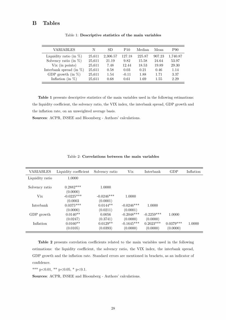
B Tables

Table 1: Descriptive statistics of the main variables

VARIABLES N SD P10 Median Mean P90Liquidity ratio (in %) 25,611 2,306.57 127.18 225.87 907.23 1,740.87Solvency ratio (in %) 25,611 21.19 9.82 15.58 24.64 53.97

Vix (in points) 25,611 7.48 12.44 18.53 19.89 29.30Interbank spread (in %) 25,611 0.58 0.03 0.21 0.46 1.14GDP growth (in %) 25,611 1.54 -0.11 1.88 1.71 3.37Inflation (in %) 25,611 0.68 0.61 1.69 1.55 2.29

Table 1 presents descriptive statistics of the main variables used in the following estimations:

the liquidity coefficient, the solvency ratio, the VIX index, the interbank spread, GDP growth and

the inflation rate, on an unweighted average basis.

Sources: ACPR, INSEE and Bloomberg - Authors’ calculations.

Table 2: Correlations between the main variables

VARIABLES Liquidity coefficient Solvency ratio Vix Interbank GDP InflationLiquidity ratio 1.0000

Solvency ratio 0.2882*** 1.0000(0.0000)

Vix -0.0225*** -0.0246*** 1.0000(0.0003 (0.0001)

Interbank 0.0375*** 0.0144** -0.0246*** 1.0000(0.0000) (0.0211) (0.0001)

GDP growth 0.0140** 0.0056 -0.2048*** -0.2259*** 1.0000(0.0247) (0.3741) (0.0000) (0.0000)

Inflation 0.0160** 0.0129** -0.1645*** 0.2023*** 0.0379*** 1.0000(0.0105) (0.0393) (0.0000) (0.0000) (0.0000)

Table 2 presents correlation coefficients related to the main variables used in the following

estimations: the liquidity coefficient, the solvency ratio, the VIX index, the interbank spread,

GDP growth and the inflation rate. Standard errors are mentioned in brackets, as an indicator of

confidence.

*** p<0.01, ** p<0.05, * p<0.1.

Sources: ACPR, INSEE and Bloomberg - Authors’ calculations.

28

Table 3: Correlation between Liquidity Coefficient and Liquidity Coverage Ratio

LCR gross LCR (LCR) Liquid assets (LCR) Cash outflowsLC 0.1851***gross LC 0.6946***(LC) Liquid assets 0.4063***(LC) Cash outflows 0.3587***

Table 3 shows the correlation between the French Liquidity Coefficient (LC) and the Basel IIILiquidity Coverage Ratio (LCR). Variables are expressed in ratio and in gross level terms.*** p<0.01, ** p<0.05, * p<0.1.Sources: ACPR, Authors’ calculations.

Table 4: Liquidity Coefficient as a good proxy for the LCR?

(1)VARIABLES Liquidity Coverage Ratio

ln_Liquid assets (LC, gross) 75.74**(27.01)

ln_Cash outflows (LC, gross) -17.31(18.08)

ln_Intragroup operations (LC, gross) -9.10**(3.80)

Constant -655.83(561.31)

Bank Fixed Effects Yes

Observations 30Number of cib 13Adjusted R-squared 0.12

Table 4 reports estimates of the regression of the level of the Basel III Liquidity Coverage Ratioon the Liquidity Coefficient components (numerator and denominator) in gross terms. Standarderrors are in brackets.*** p<0.01, ** p<0.05, * p<0.1.Sources: ACPR - Authors’ calculations.

29

Table 5: Simultaneous equations: Liquidity coefficient - Solvency ratio

(1) (2)VARIABLES Liquidity ratio Solvency ratio

Liquidity ratioi,t−1 0.625*** 8.46e−5 ***(0.005) (2.41e−5)

Solvency ratioi,t−1 5.202*** 0.891***(0.643) (0.003)

Vixt -0.124 -0.000(1.012) (0.005)

Interbankt -4.659 -0.064(13.505) (0.062)

GDPt -10.944** -0.050**(5.109) (0.023)

Inflationt 3.806 -0.119**(10.854) (0.050)

Sizei,t−1 -281.002** -0.163(129.351) (0.594)

Retaii,t−1 0.214 -0.003(0.710) (0.003)

RoEi,t−1 0.002(0.003)

2010 Dummyt -82.922*** 0.552***(22.240) (0.102)

Constant 935.021** 1.152(374.204) (1.719)

Bank Fixed effects Yes YesObservations 23,264 23,264Adjusted R-squared 0.767 0.947

Table 5 reports estimates of a system of 2 simultaneous equations with fixed effects. The twodependent variables are the liquidity coefficient and the solvency ratio, also used in lag amongexplanatory variables. The other explanatory variables include financial variables (VIX and in-terbank spread), macroeconomic variables (GDP and inflation rate), bank control variables (size,retail and return on equity ratio), a dummy variable (referring to 2010 as a change in definitionof the liquidity coefficient, with the value 1 corresponding to the period from 2010 onwards) andindividual bank fixed effects. Standard errors are in brackets.*** p<0.01, ** p<0.05, * p<0.1.Sources: ACPR, INSEE and Bloomberg - Authors’ calculations.

30

Table 6: High stress periods

(1) (2)VARIABLES Liquidity ratio Solvency ratio

Liquidity ratioi,t−1 0.625*** 8.46e−5***(0.005) (2.4e−5)

Solvency ratioi,t−1 5.186*** 0.891***(0.643) (0.003)

Vixt 0.785 -0.003(1.379) (0.006)

Interbankt -14.631 -0.362***(22.555) (0.104)

d_high_vixt 277.724* 1.434*(162.366) (0.746)

d_high_interbankt 423.997** -1.903**(171.167) (0.787)

Vixt * d_high_vixt -7.330* -0.025(4.075) (0.019)

Interbankt * d_high_interbankt -151.619** 1.166***(75.753) (0.348)

GDPt -11.442** -0.050*(5.756) (0.026)

Inflationt 5.473 -0.061(11.205) (0.052)

Sizei,t−1 -280.536** -0.216(129.384) (0.594)

Retaili,t−1 0.253 -0.003(0.710) (0.003)

RoEi,t−1 0.002(0.003)

2010 Dummyt -79.190*** 0.631***(22.701) (0.105)

Constant 933.453** 1.250(374.598) (1.720)

Bank Fixed Effects Yes YesObservations 23,264 23,264Adjusted R-squared 0.767 0.947

Table 6 reports estimates of a system of 2 simultaneous equations. The two dependent variables arethe liquidity coefficient and the solvency ratio, also used in lag among explanatory variables. Theother explanatory variables include financial variables (VIX and interbank spread), macroeconomicvariables (GDP and inflation rate), bank control variables (size, retail and return on equity ratio),dummy variables (referring to the period from 2010 onwards, to the high VIX periods and to thehigh interbank spreads periods), interaction terms and individual bank fixed effects. Standarderrors are in brackets.*** p<0.01, ** p<0.05, * p<0.1.Sources: ACPR, INSEE and Bloomberg - Authors’ calculations.

31

Table 7: Less liquid/less capitalised banks

(1) (2)VARIABLES Liquidity ratio Solvency ratio

Liquidity ratioi,t−1 0.625*** 8.25e−5***(0.005) (2.4e−5)

Solvency ratioi,t−1 5.174*** 0.890***(0.643) (0.003)

Vixt 0.875 -0.003(1.401) (0.007)

Interbankt -12.336 -0.402***(22.789) (0.106)

Vixt * d_high_vixt -7.415* -0.024(4.077) (0.019)

Interbankt * d_high_interbankt -150.454** 1.223***(75.803) (0.348)

d_high_vixt 280.442* 1.419*(162.409) (0.746)

d_high_interbankt 419.201** -1.999**(171.325) (0.787)

d_lessliqi, t -25.164(103.024)

d_undercapi, t -0.806**(0.329)

Vixt * d_lessliqi, t -0.829(4.741)

Vixt * d_undercapi, t 0.005(0.014)

Interbankt * d_lessliqi, t -26.567(61.211)

Interbankt * d_undercapi, t -0.007(0.202)

Macroeconomic variables Yes YesBank controls Yes Yes2010 Dummyt Yes YesBank Fixed Effects Yes Yes

Constant 927.588** 1.276(374.652) (1.719)

Observations 23,264 23,264Adjusted R-squared 0.767 0.947

Table 7 reports estimates of a system of 2 simultaneous equations. The two dependent variables arethe liquidity coefficient and the solvency ratio, also used in lag among explanatory variables. Theother explanatory variables include financial variables (VIX and interbank spread), macroeconomicvariables (GDP and inflation rate), bank control variables (size, retail and return on equity ratio),dummy variables (referring to the period from 2010 onwards, to the least liquid banks, to the leastcapitalised banks, to the high vix periods and to the high interbank spreads periods) and individualbank fixed effects. Columns (1) and (2) present estimates of the impact of financial variables onregulatory ratios for banks that are less liquid (liquidity coefficiento<120%) or less capitalised(solvency ratio<10%). Standard errors are in brackets. *** p<0.01, ** p<0.05, * p<0.1.Sources: ACPR, INSEE and Bloomberg - Authors’ calculations.

32

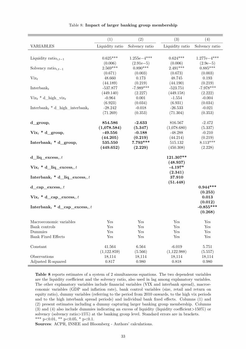
Table 8: Impact of larger banking group membership

(1) (2) (3) (4)VARIABLES Liquidity ratio Solvency ratio Liquidity ratio Solvency ratio

Liquidity ratioi,t−1 0.625*** 1.255e−4*** 0.624*** 1.277e−4***(0.006) (2.91e−5) (0.006) (2.9e−5)

Solvency ratioi,t−1 2.569*** 0.890*** 2.491*** 0.885***(0.671) (0.003) (0.673) (0.003)

Vixt 48.660 0.173 48.745 0.193(44.189) (0.219) (44.190) (0.219)

Interbankt -537.877 -7.989*** -523.751 -7.978***(449.140) (2.227) (449.158) (2.222)

Vixt * d_high_vixt -0.964 0.001 -1.554 -0.004(6.923) (0.034) (6.931) (0.034)

Interbankt * d_high_interbankt -28.242 -0.018 -26.533 -0.021(71.269) (0.353) (71.304) (0.353)

d_groupi 854.586 -2.633 816.567 -2.472(1,078.584) (5.347) (1,078.680) (5.337)

Vixt * d_groupi -49.556 -0.188 -48.288 -0.210(44.205) (0.219) (44.214) (0.219)

Interbankt * d_groupi 535.550 7.793*** 515.132 8.113***(449.652) (2.229) (450.308) (2.228)

d_liq_excessi, t 121.307**(48.937)

Vixt * d_liq_excessi, t -4.197*(2.341)

Interbankt * d_liq_excessi, t 37.910(51.448)

d_cap_excessi, t 0.944***(0.253)

Vixt * d_cap_excessi, t 0.013(0.012)

Interbankt * d_cap_excessi, t -0.855***(0.268)

Macroeconomic variables Yes Yes Yes YesBank controls Yes Yes Yes YesDummies Yes Yes Yes YesBank Fixed Effects Yes Yes Yes Yes

Constant 41.564 6.564 -6.019 5.751(1,122.859) (5.566) (1,122.988) (5.557)

Observations 18,114 18,114 18,114 18,114Adjusted R-squared 0.817 0.980 0.818 0.980

Table 8 reports estimates of a system of 2 simultaneous equations. The two dependent variablesare the liquidity coefficient and the solvency ratio, also used in lag among explanatory variables.The other explanatory variables include financial variables (VIX and interbank spread), macroe-conomic variables (GDP and inflation rate), bank control variables (size, retail and return onequity ratio), dummy variables (referring to the period from 2010 onwards, to the high vix periodsand to the high interbank spread periods) and individual bank fixed effects. Columns (1) and(2) present estimates including a dummy capturing larger banking group membership. Columns(3) and (4) also include dummies indicating an excess of liquidity (liquidity coefficient>150%) orsolvency (solvency ratio>15%) at the banking group level. Standard errors are in brackets.*** p<0.01, ** p<0.05, * p<0.1.Sources: ACPR, INSEE and Bloomberg - Authors’ calculations.

33

Table 9: Heterogeneity between banks’ types

(1) (2)VARIABLES Liquidity ratio Solvency ratio

Liquidity ratioi,t−1 0.624*** 1.323e−4***(0.006) (2.91e−5)

Solvency ratioi,t−1 2.687*** 0.888***(0.675) (0.003)

Vixt 0.645 -0.051***(2.604) (0.013)

Interbankt -77.473 0.688**(56.545) (0.280)

Vixt * d_high_vixt -1.211 -0.003(6.924) (0.034)

Interbankt * d_high_interbankt -27.540 0.019(71.288) (0.353)

d_fini 114.486 -0.114(187.415) (0.929)

Vix_d_fini, t -0.124 -0.006(4.784) (0.024)

Interbank_d_fini, t 37.890 -1.276**(113.938) (0.565)

d_comi 185.205 -1.964***(148.673) (0.738)

Vix_d_comi, t -3.407 0.076***(3.110) (0.015)

Interbank_d_comi, t 131.496* -1.830***(67.173) (0.333)

d_muti 71.755 -0.043(425.354) (2.108)

Vix_d_muti, t -0.646 0.032**(3.177) (0.016)

Interbank_d_muti, t 74.496 -0.423(70.704) (0.353)

Macroeconomic variables Yes YesBank controls Yes YesDummies Yes YesBank Fixed Effects Yes Yes

Constant 900.328*** 4.173***(313.734) (1.555)

Observations 18,114 18,114Adjusted R-squared 0.790 0.953

Table 9 reports estimates of a system of 2 simultaneous equations. The two dependent variables arethe liquidity coefficient and the solvency ratio, also used in lag among explanatory variables. Theother explanatory variables include financial variables (VIX and interbank spread), macroeconomicvariables (GDP and inflation rate), bank control variables (size, retail and return on equity ratio),dummy variables (referring to the period from 2010 onwards, to the high vix periods, to the highinterbank spread periods and to the types of bank) and individual bank fixed effects. Columns(1) and (2) present estimates of the interaction between financial variables and regulatory ratiosdepending on the type of bank (commercial, mutual banks or financial firms). Standard errors arein brackets.*** p<0.01, ** p<0.05, * p<0.1.Sources: ACPR, INSEE and Bloomberg - Authors’ calculations.

34

Table 10: Simultaneous equations: Liquid assets - Cash outflows - Solvency ratio

(1) (2) (3)VARIABLES Liquid assets Cash outflows Solvency ratio

Liquid assetsi,t−1 0.577*** 0.004** 0.003(0.006) (0.002) (0.002)

Cash outflowsi,t−1 0.200*** 0.794*** 0.004(0.014) (0.004) (0.005)

Solvency ratioi,t−1 0.110*** -0.010*** 0.892***(0.008) (0.002) (0.003)

Vixt -0.010 -0.000 -0.003(0.017) (0.005) (0.006)

Interbankt -0.795*** -0.319*** -0.351***(0.285) (0.084) (0.104)

Vixt * d_high_vixt 0.005 0.011 -0.026(0.051) (0.015) (0.019)

Interbankt * d_high_interbankt 0.874 0.920*** 1.168***(0.957) (0.281) (0.348)

GDPt -0.250*** 0.037* -0.051*(0.073) (0.021) (0.026)

Inflationt 0.078 0.121*** -0.061(0.142) (0.042) (0.052)

Sizei,t−1 -0.386 0.670 -0.209(1.634) (0.480) (0.594)

Retaili,t−1 -0.080*** -0.011*** -0.002(0.009) (0.003) (0.003)

RoEi,t−1 0.002(0.003)

Dummies Yes Yes YesBank Fixed Effects Yes Yes Yes

Constant 12.610*** 0.812 1.437(4.730) (1.389) (1.720)

Observations 23,264 23,264 23,264Adjusted R-squared 0.833 0.906 0.947

Table 10 reports estimates of a system of 3 simultaneous equations. The three dependent variablesare the numerator of the liquidity coefficient (Liquid assets), the denominator of the liquidity coeffi-cient (Cash outflows), both normalized, and the solvency ratio, also used in lag among explanatoryvariables. The other explanatory variables include financial variables (VIX and interbank spread),macroeconomic variables (GDP and inflation rate), bank control variables (size, retail and returnon equity ratio), dummy variables (referring to the period from 2010 onwards, to the high vixperiods and to the high interbank spreads periods) and individual bank fixed effects. Standarderrors are in brackets.*** p<0.01, ** p<0.05, * p<0.1.Sources: ACPR, INSEE and Bloomberg - Authors’ calculations.

35

C Annex: more detailed analysis of the theoretical model

C.1 Set-up of the model and assumptions

The main objective of our model is to assess how banks react to liquidity shocks. We study the

determinants of bank’s liquidity and its interaction with market liquidity. Our model is based on a

representative bank that maximises its profit under balance sheet, capital and liquidity constraints.

Two sources of financing are available to the bank: equity capital, denoted K; and debt D,

remunerated at the ex ante fixed rate rd. Depending on the state of the economy, a fraction α of

deposits is withdrawn.

There are two items on the asset side: loans L, with a long-term maturity and expected return

rl; and marketable securities G, whose return rg is equal to the risk-free rate.

It can be illustrated by a look at the structure of a bank’s balance sheet:

Assets = A Liabilities =LBTL rl D rd

G rg K rk

Total = A Total = A = LBT

We assume the following inequalities: rg < rd < rl. Loans are considered to be riskier and,

thus, provide a higher rate of return. K is assumed to be exogenous.

Bank’s profit. The bank is assumed to behave as a mean-variance investor with risk aversion

coefficient γ. The profit can be written as the following, with a risk-return arbitrage term as in

Freixas and Rochet (2008) and in Fraisse et al. (2019), among others:

maxG,L,D

π = rlL+ rgG− rdD − γ

2 (σ2GG

2 + 2σGLGL+ σ2LL

2) (10)

with σ2G and σ2

L being the variance of returns on securities and loans, respectively, and σGL the

covariance between the returns on securities and loans.

Bank’s constraints. The bank faces three different constraints.

• The first one is a balance sheet constraint:

D +K = L+G (11)

For a given level of total assets, this balance sheet constraint implies that the larger the capital K,

the lower the debtD, hence the lower the risk of deposit outflows. From that point of view, solvency

regulation, which aims at increasing K, and liquidity regulation, which aims at reducing D, may

appear as substitutable. However, we will see below that they may arise more complementary than

substitutable.

• The second one is a solvency constraint, defined as capital over risk-weighted assets:

K ≥ wL L+ wG G with 0 < wG < wL < 1 (12)

36

• The third one is a liquidity constraint, close to the LCR regulatory definition:

G ≥ α D, (13)

where αD are the deposit outflows, with α > 0. It can also be the expected level of haircuts

on G when the bank needs to sell the bonds to meet deposit withdrawals.

Plugging the balance-sheet constraint into the liquidity constraint yields:

G ≥ α (L+G−K) (14)

Assuming that the solvency constraint is binding, the liquidity constraint becomes becomes:

G ≥ α(L+G− wLL− wGG) = α((1− wL)L+ (1− wGG)) (15)

or:

G(1− α(1− wG) ≥ α(1− wL)L (16)

which implies

G[ 1− α(1− wG)α(1− wL) ] ≥ L = (A−G)⇒ G ≥ ([1− α(1− wG)

α(1− wL) ] + 1)−1A = Â (17)

Note that:

1− α(1− wG)α(1− wL) ≥ 0⇒ Â ≤ A (18)

and the constraint becomes:

 ≤ G ≤ A (19)

The constraint is tightened when α increases since:

∂Â∂α

= (1− wL)A[ 1−α(1−wG)α(1−wL) + 1]2

> 0 (20)

Similarly, an increase in wL which implies a reduction in L leads to a softening of the constraint:

∂Â∂wL

< 0 (21)

It is therefore possible to conclude that solvency and liquidity are to some extent substitutable

in the sense that the constraint is tightened with either an increase in α or a decrease in wL,

leading to an increase in G (of course an overall increase in solvency requirement would also have

an effect on G, hence would have an additional impact on deleveraging).

C.2 The programme of the bank

We are interested in identifying the determinants of the share of marketable securities G. The

bank maximises its profit; its variables of choice are G, L and D, conditional on a level of total

37

liabilities (K +D, assuming the solvency constraint holds):

maxG,L,D

π = rlL+ rgG− rdD − γ

2 (σ2GG

2 + 2σGLGL+ σ2LL

2) (22)

subject to the transformed liquidity constraint:

G ≥ Â (23)

and

L+G = A⇔ L = A−G (24)

We can associate the following Lagrangian function, with D and K, hence A exogenous:

L(G) = rl(A−G) + rgG− rdD

−γ2

(σ2GG

2 + 2σGLG(A−G) + σ2L(A−G)2

)+λ(G−Â) (25)

with λ the Lagrange multiplier of the liquidity constraint.

The first-order condition of the Lagrangian on G is the following:

∂L∂G

= 0⇔ −rl + rg − γ

2

(2σ2

GG+ σGL(A− 2G)− 2σ2L(A−G)

)+ λ = 0 (26)

⇔ −(rl − rg)− γ(σ2G − σ2

GL + σ2L)G− γ

2 (σGL − 2σ2L)A+ λ (27)

After solving the first-order condition, we get the following expression of G:

G∗ =γ(σ2

L −σGL

2 )A− (rl − rg) + λ

σ2G + σ2

L − σGL(28)

Similarly, using 24, one gets:

L∗ =[σ2G − (1− γ

2 )σGL + (1− γ)σ2L]A+ (rl − rg)− λ

σ2G + σ2

L − σGL(29)

From these two equations, it is clear that when the liquidity constraint is binding (λ>0), the

demand for G increases and the demand for L decreases. The covariance term σGL (for σGL > 0)

mitigates partially this effect (when γ > 2).

The conclusions at this stage, is that:

liquidity requirement implies a further deviation from the Markowitz portfolio, hence imply a

reduction in profitability.

transposing the analysis into Hoerova et al. (2018)’s framework, this implies an increase in the

probability of failure; we get the same conclusion as Hoerova et al. (2018), generalising their result

in a mean-variance setup.

38

C.3 Ex post analysis and run probability

Beyond the ex ante analysis of the analysis, it is useful to consider ex post analysis, once the shock

on risky asset has materialised. This allows us to assess the risk of failure as well as the risk of the

run.

We cast our analysis in the framework proposed by Hoerova et al. (2018). Two simplifications

are needed. First, the liquid asset G is a risk-free asset, although this assumption is dropped later.

Second, the risk aversion component disappears as uncertainty has materialised.

The return on the risky asset is subject to a shock ω. The timing is as follows: at the beginning

of the period the bank offers deposit contracts and invests in the risky asset L as well as the safe

asset G. At the end of the period, the bank pays a return rd to depositors. The return on the risky

asset is subject to a stochastic shock ω.

Ex-post profit, i.e. at the end of the period, is defined, consistently with our previous definition,

as:

π = ωRlL+ rgG− rdD (30)

where 0 ≤ ω ≤ 1 is the realisation of the shock on the risky asset L, Rl is the maximum

realisation of the return on the risky asset, so that E(ωRl) = rl, hence E(ω) = rl

Rl .

Profit is subject to the same constraints as before and we consider that the last two also hold

with equality:

D +K = L+G (31)

K = wL L+ wG G (32)

G = α D, (33)

C.3.1 Bank Failure probability

Following Hoerova et al. (2018), it is easy to see that profit is positive if:

ω ≥ (rd − αrg)rl

(1− wL)(1− α(1− wG)) (34)

∂ω

∂α= [(1− wG)rd − rg]

[1− α(1− wG)]2(1− wL)

rl> 0 (35)

A tighter LCR regulation (α increases) increases the probability of failure (ω increases) by

reducing profits.

C.3.2 Probability of run

To assess the effect on depositors’ run, we assume that:

• the bank invests in the risky asset at the beginning of the period. If it needs to liquidate the

asset before the end, it has to pay a cost of µ;

39

• following Bhattacharya and Jacklin (1988) and Hoerova et al. (2018), depositors receive the

promised return on their deposit on a first-come first-served basis. Some informed depositors,

representing a share χ of depositors, receive a signal before the end of the period, which may

induce them to go to the bank to withdraw their deposit. They will never do that if the

signal is that ω is high enough. They will do that if the signal indicates that the bank will

not be able to meet its obligations. If these depositors withdraw their deposits, the bank has

to liquididate the risky asset.

The run probability is given by the realisation of ω for which the informed depositors expect

that the bank will not have enough resources to provide the expected return.

ωRl(1− µ)L+ rgG < rdDχ (36)

The threshold is such that:

ω ≤ Rl(1− µ)L+ rgG < rdDχ (37)

which yields:

ω <rd(χ− rG

rd α)(1− wL)Rl(1− µ)(1− α(1− wG)) = ω (38)

∂ω

∂α= (χ(1− wG)− rG

rd) rd(1− wL)Rl(1− µ)[1− α(1− wG)]2 (39)

This expression is negative for χ small, so that a tightening of the liquidity constraint implies

a lower threshold value.

As the safe asset does not bear liquidation costs, the existence of a liquidity buffer helps reduce

the probability of runs.

C.3.3 Extension of the model to haircut risk

An extension of the model is to include haircuts when liquidating the sovereign bonds. The

extended liquidity constraint (40) still ensures that banks accumulate enough liquid assets to

be able to cope with net cash outflows (deposit outflows, debt roll-off). To cope with deposit

withdrawals at time t, the bank must sell marketable securities to get cash. However, depending

on the market liquidity and the state of the economy, marketable securities are not necessarily sold

at their book value, which affects the bank’s liquidity position.

(β + (1− β)φ)G ≥ α D, (40)

where 0 ≤ β ≤ 1 is the share of marketable securities maturing in the current period, so that

(1−β) measures the average bank’s holdings of longer horizon bonds. Liquidating the latter bonds

implies a haircut of (1− φ), hence 0 ≤ φ ≤ 1 is a fraction of the book value of the securities which

were not maturing at t, i.e. a measure of the liquidity of the bank’s marketable securities which is

state-dependent.

40

It is easy to see that such a sovereign bond buffer will not be as powerful to deter informed

depositors from withdrawing deposits.

41