Determinants and Consequences of Agroforestry:Historical Evidence from the Great Plains Shelterbelt

Project∗

Aparna Howlader†

November 30, 2020

Abstract

This paper examines the determinants and consequences of the adoption of large-scale tree plantation projects on farmland using the experience of the Great PlainsShelterbelt Project in the late 1930s. I show how market pressure influenced thedecision to plant shelterbelt trees on the cropland, and how soil erosion has changedin the long run because of the large-scale tree plantation. I consider world marketprice movement, initial crop production intensity, and the 100-mile-wide shelterbeltproject planning belt to examine the determinants of the adoption. The main findingis that an increase in the market crop price reduces the adoption of shelterbelt trees,and that agricultural factors such as tenancy, access to irrigation, and durationof the agricultural contract explain the variations in the decision process. Also,shelterbelt adoption decreases long-term wind erosion, especially in pasture areas.

Keywords: Land Conservation, Soil Erosion, Windbreak, Agricultural History

JEL Codes: N52, N92, Q15, Q18, Q57

∗I thank the National Archives at Kansas City, Missouri for giving me access to the annual reportson the Prairie State Forestry Project. I am extremely grateful to Patrick Flanagan from the UnitedStates Department of Agriculture for creating a county-level erosion database from the Natural ResourceInventory. I acknowledge financial support from the Economic History Association. All remaining errorsare my own.†Postdoctoral Research Associate, The Eviction Lab, Princeton University; howlader@princeton.edu

1 Introduction

Private farmland conservation, especially agroforestry, has been widely adopted as

a farmland conservation instrument all over the world (Schoeneberger, 2009). Many

agricultural science experiments examine how tree plantation projects help to achieve

long-term environmental sustainability and increase community resilience (Young, 1989;

Nair, 1993; Beetz, 2011). Based on these experimental results, the recent social science

and ecology literature has included studies on how to give incentives to farmers to adopt

agroforestry on their farmland in developing countries (Brown et al., 2018; Miller et al.,

2020; Scherr, 1992; Mercer and Pattanayak, 2003; Woodruff, 1977). However, trees need

time to affect the environment, and due to the lack of sufficient long-term data relating

to large-scale tree plantation in developing countries, it has been difficult to understand

the determinants of adoption in agroforestry and the consequences of tree plantation on

farmland over time. Historical projects related to large-scale tree plantations may help

us to understand the costs and benefits associated with large-scale tree plantation projects.

The success of any large-scale tree plantation program depends on farmers’ initial

uptake rate and their persistence in maintaining trees over time. The benefit associated

with tree plantation is not immediately visible, and so, farmers have few incentives to

plant and take care of trees on their farmland. Production and conservation are com-

peting demands for agricultural land use, and this problem is enhanced in large-scale

tree plantation programs. First, scattered trees over the landscape cannot solve the

problems related to land degradation. Erosion will only be reduced by continuous tree

bands, for which it is necessary to convert a large number of continuous farm plots. This

involves a collective action problem for the farmers who need to come to a joint farm plan.

Second, property rights and institutional frameworks also influence the decision process.

Farmers struggle to decide for long run because of the incomplete information about the

benefits of tree plantation, and other institutional barriers such as tenancy reduce the

probability of planting trees for the long-term benefits. Understanding what determines

farmers’ adoption decision on a large-scale plantation program is important because it

1

helps planners to design incentives in the future projects (Hughes et al., 2020).

Despite the importance of understanding the adoption of farmland conservation

instruments under market pressure, economic studies on the effects have been limited

because of data limitations. This paper examines these questions using the example of one

of the earliest and most popular tree plantation programs in the United States, the Great

Plains Shelterbelt Project. Large-scale agroforestry projects have historical roots in Stalin’s

Great Plan for the Transformation of Nature or Roosevelt’s Great Plains Forestry Project

(Brain, 2010; Gardner, 2009). Recent examples of large-scale agroforestry projects include

the Three North Shelterbelts in China and the Great Green Wall in the Sahara Desert (Li

et al., 2012; Aigbokhaevbo, 2014). In this paper, using historical data and policy design,

I answer these two questions: what factors determine decisions relating to tree planta-

tion on the farmland, and how does tree plantation affect long-term environmental quality?

The uniqueness in designing the Great Plains Shelterbelt Project, the size of the

program, the nature of the public-private partnership, and the availability of the data in

the National Archives and Records Administration (NARA) make this plantation project

a perfect case study to understand the determinants and consequences of such projects.

In the Dust Bowl era, Franklin D. Roosevelt introduced the idea of planting shelterbelts,

and the U.S. Forest Service (USFS) was responsible for implementing it. At first, USFS

asked farmers to sell the land at a low cost, but farmers did not respond to the incentive.

Later on, it was converted to a public-private partnership, where farmers were responsible

for clearing their land and government was responsible for helping to decide tree species

and providing technical support. USFS planted 220 million trees from 1935 to 1942 across

the Great Plains (Droze, 1977)

To study the factors behind tree plantation, I digitize unique county-year panel data

on annual shelterbelt plantation acres for 1936-1940 available in the NARA. I take advan-

tage of detailed county-level annual farm forestry plantation data from the shelterbelt

2

project annual reports deposited in the National Archives at Kansas City, Missouri. I

overlay this data with county-level crop intensity data from the pre-Dust Bowl era, and

thus, I create a spatial variation in crop intensity. I interact this spatial variation with

temporal price shock to see how a change in crop prices affect tree planting. Also, I show

that other pre-Dust Bowl variables do not differ between shelterbelt and non-shelterbelt

counties. This unique database provides the option to study the impact of commodity

price on shelterbelt adoption behavior in detail.

Moreover, I show how county-level shelterbelt trees reduced soil erosion levels in the

shelterbelt counties compared to non-shelterbelt areas. I utilize the setting to show that

farms have a long-run effect on the erosion from this adoption behavior. To understand

the impact of this plantation project on the environment, I draw on the Natural Resource

Inventory database from the U.S. Department of Agriculture (USDA) to shed light on the

impact of shelterbelt plantation on county-level erosion control in the long run. To deal

with endogeneity concerns about the plantation decision, I use the planning map for the

100-mile-wide shelterbelt project to create a pre-plantation treatment and control group

based on geographic differences (Li, 2019)

The results show that price increase had a negative effect on the adoption of agro-

forestry practices in the 1930’s. Descriptive statistics show that the other variables did not

change over the shelterbelt counties, and the results are robust to different county-level

controls. The results from historical data support the theory that price fluctuation affected

the initial take-up rate. Using a triple difference model, I show how heterogeneity in the

initial agricultural institutions affects the adoption decision. I show how tenancy, duration

of agricultural contract, access to alternative resources, and number of farms affect the

decision. I also show how access to farm trees before the shelterbelt project affect the

plantation decision.

Results from the effect of the tree plantation project, in the long run, suggest that

3

shelterbelt decreases erosion level in the areas in which profits were limited from initial

uptake, and that the effects are largest in pasture areas. This supports the results of Li

(2019) that agricultural revenue mostly increased in pasture areas because of the tree

plantation. I show the persistent environmental effects of the shelterbelt on both pasture

and cropland. We see that shelterbelts help to reduce wind erosion in these areas even

after eighty years.

This paper contributes to the agricultural economics literature on farmers’ tree

adoption behavior under market pressure and the impact of the adoption in the long

run. Studies show that prices of output play an important role (Adesina and Zinnah,

1993;Reimer, Gramig, and Prokopy, 2013;Prokopy et al., 2019). The literature on tree

plantation projects also shows how spatial variation affects the progress (Elkin, 2014;

Bellefontaine et al., 2011). This paper contributes to this literature by using a historical

case to show how evaluating market pressure is important to understand the impact of

the policy when landowners are volunteering to adopt conservation practices. This paper

also shows how historical conservation policies affect current environmental and economic

outcomes (Hornbeck, 2012; Howlader, 2019; Li, 2019).

This paper also contributes to the growing body of economic history literature that

address environmental problems. Recent economic history papers develop insights about

how current conditions are path dependent on early historical events (Hornbeck, 2012).

Empirical studies have been conducted on policies related to air pollution (Cohen et al.,

2017), floods (Hornbeck and Naidu, 2014), drought (Freire-Gonzalez, Decker, and Hall,

2017), water management (Hornbeck and Keskin, 2014), and waste management (Alsan

and Goldin, 2015). In this paper, I provide the first evidence of how early tree plantation

projects have changed environmental outcomes in the long term.

This paper also contributes to the growing literature on compiling new data sources

and understanding the New Deal. Recently, empirical economists studied many facets of

4

the New Deal because of the availability of detailed county-level data over a long period

(Fishback, 2017). Accordingly, I compile and digitize new data sources and explore a new

dimension regarding the shelterbelt projects. I constructed a new database, digitizing

shelterbelt data from the National Archives.

The paper proceeds by providing background and data construction in Section 2.

Section 3 is on the empirical framework. Section 4 demonstrates the results and discussion.

Concluding remarks are in Section 5.

2 Background and Data Construction

Tree plantation was part of the policy discussion from the beginning of American

conservation policies through the 1873 Timber Culture Act. However, this was mostly a

failed attempt (McIntosh, 1975) back in that time in Nebraska and Kansas. In the 1930s,

the Dust Bowl substantially decreased the amount of topsoil in the Great Plains, and

as a result, Roosevelt promised to create the tree belt in the Great Plains, with other

conservation programs administrated by the USDA.

The shelterbelt project was planned based on Roosevelt’s previous experience with

agroforestry in Hyden Park in New York (Droze, 1977). Roosevelt posted a plan for a

continuous tree belt across the region, but the Forest Service Agency said it was scientif-

ically not viable. This plan was first proposed in 1934, and after three different plans,

the federal government passed it in 1935. Initially, the federal government leased land

from its owners for the long term. But eventually, it became tough to get the budget for

the shelterbelt. So, the government converted the program to a cost-sharing program

with landowners, where landowners were responsible for clearing the land, fencing it,

and for rodent control. The planning was based on climate and pre-program geographic

characteristics. The actual shelterbelt planting started in 1935 and ceased in 1942, as

funds were cut after the United States entered World War II (Droze, 1977).

5

The main database I used for the analysis came from the National Archives in Kansas

City. It provides plantation data that shows how much land was under plantation every

year from the beginning of the plantation project. I digitized the county reports to extract

this information. Some data came from agricultural censuses, such as tenancy, crops, and

farm size (Haines, 2010). I also used county-level initial crop intensity data from the

agricultural census. Crop price information came from Jacks (2017). I used the shelterbelt

planning data from Li(2019).

For the long-term analysis of the environment, I used erosion data from 2012 from

the natural resource inventory (NRI) database created by the United States Department

of Agriculture. I used data on the total erosion rate, total wind erosion rate, erosion on

cropland, and pastureland.

3 Empirical Strategy

3.1 Determinants of Adoption

In this section, I describe the strategy to examine the effect of price shocks on the

adoption of tree plantation. I study the underlying characteristics of adoption with the

help of pre-1930 data to see which counties have higher adoption rates. Because it was a

voluntary program, I use a difference-in-difference model to deal with potential endogeneity.

First, I study the implications of commodity price movement on shelterbelt adoption.

The plantation area denotes my outcome variable by county and year; my main exogenous

variation is the interaction of annual price movement and initial county-crop specific

intensity that came from 1930s census data.

Using newly digitized data on county-level shelterbelt plantation, I compare counties

6

with high cash crops with those with low cash crop production intensity to see how

market price affects farmers’ conservation decisions. I use data from the beginning of the

shelterbelt plantation project, 1935 and estimate:

yc,t = αc + δt + βCrop Intensity)c,1930 ∗ (Pricet) + εc,t (1)

yc,t is the outcome variable of interest in county c at the shelterbelt project period.

This model shows how the interaction of market price movement with county-level initial

crop intensity affected shelterbelt plantation decision.

County fixed effects absorb county-specific time-invariant heterogeneities affecting

the local extent of adoption. δt is the time fixed effect capturing common trend. I do not

cluster data by states because the groups are small. Identification strategy relies on the

fact that shelterbelt counties would be on the same trend as non-shelterbelt counties if

there were no plantation project.

Next, I extend this model to the triple difference model to include the heterogeneous

treatment effect from initial characteristics. I estimate the model using variations in initial

tenancy, duration of agricultural contract, irrigation, area under wood, and number of

farms. I estimate a panel regression model where H denotes these heterogeneities:

yc,t = αc + δt + β(Crop Intensity)c,1930 ∗ (Pricet) + γ(Crop Intensity)c,1930 ∗ (Pricet) ∗H + εc,t

(2)

3.2 Environmental Impact of Tree Plantation

Next, I turn the analysis to understand the impact of the tree plantation projects on

the environmental outcomes. I use the erosion rate in cropland, pastureland, and total

land erosion in 2012 as the environmental outcome. Using the data on total shelterbelt

7

plantation in any county in the 1930s, I compare erosion rates in counties with larger

plantation areas against those with smaller plantation areas. I estimate a cross-sectional

OLS equation:

yc = αc + β(Plantation)c,1940 + δXc,1940 + εc (3)

where yc is the environmental outcome. I exploit the exogenous planning map for the

shelterbelt across counties to address the endogenous adoption of tree plantation. I use a

digitized map from Li (2019). The shelterbelt planning map came from Droze (1977). It

relies on geographic conditions, and it can be used as an exogenous variation for actual

tree plantation (Li, 2019). The first-stage intuition is that higher plantation happened in

these planning areas. There were 158 counties in planning, but 218 counties in the actual

plantation.

With the help of these two models and detailed county-level adoption and erosion

data, I show how market pressure affects farmers’ conservation adoption decision, and

how the variation still dominates the environmental quality.

4 Summary Statistics

Table 1 shows the covariate balance between with- and without-shelterbelt counties.

Baseline factors are very similar in shelterbelt and non-shelterbelt counties. Mean total

shelterbelt areas for shelterbelt counties is 62 miles, and standard deviation is around 82

miles. Shelterbelt counties are less densed than non-shelterbelt counties. The population,

number of farms, size of farms, and farm values are not significantly different in shelterbelt

and non-shelterbelt counties. This effect remains even after controlling for state fixed

effects. As shelterbelt counties are less populated than other counties, the farm number is

smaller, and the average farm acreage is also smaller. There were 218 shelterbelt counties.

8

We use 434 remaining counties in the non-shelterbelt areas.

Table 2 presents the summary statistics for annual crop plantation data and crop

prices over time. We see that the areas under different crops decreased over time. This

decrease may come from the conservation projects, or the loss in harvest areas due to

the drought. We see this variation is highest in wheat counties. The targeted areas for

conversion was skewed in the wheat areas which may explain this variation.

Table 3 presents the summary statistics of annual plantation data for shelterbelts.

We see that there is a strong annual variation of adoption of shelterbelt areas. The

plantation has been continued in 1941 too, but we do not have the data in the National

Archives. I use this annual variation in the shelterbelt plantation in a panel setting to see

how much effects come from annual variation in market prices for the crops.

5 Results

Table 4 presents the results for the determinants of the adoption related to mar-

ket pressure. Table 5 shows the results using heterogeneous treatment effect analysis

where I use initial county characteristics to explore the variations. There were three

main crops in the Great Plains in 1930, and every row represents one crop. Next, we

move toward the discussion of the long-term effects of the trees on environmental outcomes.

5.1 Determinants of Adoption

The main finding of this section is that Great Plains farmers who could obtain higher

market prices for their crops converted less of their land to shelterbelts. Table 4 shows

these results using regression model 1.

First set of results show farmers facing higher crop prices planted less shelterbelt.

9

I use five years of panel data for this set of results. If we convert the estimates based

on average plantation, first, farmers facing a 1-unit increase in corn price and having 1

unit of additional intensity in initial corn production planted 0.38 miles less shelterbelt.

Second, farmers facing a 1-unit increase in cotton price and having 1 unit of additional

intensity in initial cotton production planted 5.89 miles less shelterbelt. Third, farmers

facing a 1-unit increase in wheat price and having 1 unit of additional intensity in initial

wheat production planted 0.11 miles less shelterbelt.

These results correspond to the intuitive understanding that farmers react to market

prices to abandon land for long-term conservation purpose. If the price is high, farmers

plant less shelterbelt trees. The results are crop specific following price dynamics in Figure

1. Next, I use initial county characteristics to explain the spatial variations in some of

these results.

Next, Regression Model 2 shows heterogeneous effects from initial county-level insti-

tutional and farm characteristics. These results follow the theoretical concepts regarding

the interrelationships among agroecological, economic and social variables. They show

how farmers’ decisions on shelterbelt plantation depended on agrarian institutions. I used

the triple difference model as presented in regression model 2. Table 5 presents these results.

First, theoretically, if a farm is under a tenancy contract, it may or may not have

a higher adoption rate. On one hand, we need more farm labor to plant more trees, so

more tenants may help to plant more trees. On the other hand, tenant-dependent farms

may have a lower attachment to farming in general, so it may have a lower adoption

rate as farmers cannot see the benefit of tree plantation immediately. Column 1 of Table

5 shows these results. For cotton, where the farms were very much tenant dependent,

more tenants helped to adopt more trees. But for corn, the adoption rate was lower

than average. There were no significant results for wheat. This result is important to

understand the elasticity of substitution between land and labor given the choice of

10

tree plantation. In a very labor intensive crop plantation like cotton, tenants help to

plant more shelterbelts too. But in places where crops are less labor intensives, tenants

probably focus on planting crops and shelterbelt is not the priority project for limited time.

Second, I use duration of agricultural contract to see if farmers’ movement affect tree

plantation. Column 2 of Table 5 shows that contract duration only affected plantation

decisions in corn counties, and that the effect was positive. If the duration is higher, it

means a higher adoption rate for corn-intensive counties. I took the average number of

years on one farm as the duration of the contract. Interestingly, even if farmers tenancy

rate affected tree plantation on cotton farms, it did not have any relationship with contract

duration. The reason may lie in the fact that cotton tenants are mostly sharecroppers

who still used to live on the farms for a long time.

Third, I use areas under alternative access to water as another source of heterogene-

ity. If farmers have more access to irrigation, the chances to rely on shelterbelt for soil

moisture is low. Column 3 of Table 5 shows that irrigation has a negative effect on tree

plantation in wheat counties. Wheat is a highly water-dependent crop compared to other

crops. Wheat needs more irrigation, and that may crowd out shelterbelt plantation as the

results suggest. We do not see any significant effect in corn and cotton counties in this case.

There is also information on total existing wood acreage in 1934 before the shelterbelt

project started. Existing wood acreage may have a positive effect on more plantation as

farmers may already have knowledge about plantation. That result is in Column 4. The

result is significant and positive only for cotton counties. Wood in 1934 was skewed in the

southern states, so the results are spatially concentrated in that area. The underlying

intuition is correct that access to farm plantation before the project helped to plant more.

This is similar to additionality effect.

Fifth, the number of farms may have an effect on shelterbelt plantation due to

11

coordination failure, as tree band involves a collective action problem from the farmers.

Column 5 shows that there are no significant effects from the number of farms.

5.2 Consequences of Adoption

The main finding in this section is that the plantation of shelterbelt decreases pasture

wind erosion. I used the shelterbelt planning map as the instrumental variable for the

actual plantation acres (Li, 2019). I expected the effects from the omitted variables to

drive the results up, and the results are consistent with this expectation.

I use variables from Natural Resource Inventory on total erosion, total wind erosion,

erosion on pastureland, and erosion on cropland. I do not use data for water erosion. I

use the data from 2012. The idea is to see the persistent effect of shelterbelt projects on

the erosion in the long run.

Table 6 presents the results for total erosion in shelterbelt counties. The first column

presents the results for Regression Model 3. It shows that there is no effect of plantation

on total erosion. Then, I used the instrumental variable from Li (2019) following Model

3. The results of the first and second stage are in Columns 2 and 3. We do not see a

significant effect of tree plantation on total erosion even after using the instrumental

variables. The results are similar for other years too. Comparable results for total wind

erosion are in Table 7, and the results are still not significant after using the instrumental

variable.

Next, I present the results for the total pastureland erosion in Table 8. Column 3

shows the results. In this case, we see that the results show shelterbelt had a persistent

negative effect on wind erosion. If counties had more exposure to shelterbelt plantation in

1940s, they still have lower erosion rate in the pastureland. Shelterbelts were primarily

adopted in the pastureland, so the results are consistent with the anecdote.

12

Table 9 present results for the wind erosion rate on the pastureland. We see that

the plantation area decreases the wind erosion rate on the pastureland after using the

instrumental variable. From a scientific perspective, this is true, as shelterbelt mostly

helped and was planted in livestock areas (Li, 2019).

Next, in Table 10, I present results for cropland erosion. Shelterbelts also decreased

erosion on the cropland in the long run. This may come directly as a result for shelterbelt

plantation, or through the decrease of pasture erosion.

These results have important policy implication. I show that shelterbelt tree plan-

tation has a persistent effect on soil even after 80 years. The project may have been

disrupted with market variation and other temporal variables, but the consistent effect on

the environmental outcomes is important to think about long-term project planning like

this.

6 Conclusion

This paper studies the influence of market price in the adoption of conservation

projects taking the example of large-scale tree plantation in the Great Plains. It shows

that the market price was a big factor in adoption, and also show how initial agrarian

structure have an effect on the adoption. I also show how plantation helped to reduce

pastureland soil erosion in the long run.

These findings are significant for both developed and developing countries working

on conservation programs. First, policymakers, while designing policy to give farmers

incentives to adopt farmland conservation practices, need to consider the effect of the

price dynamics in the commodity market. If farmers expect a higher crop price, they will

stop planting more trees. In this case, policy makers may adjust the incentive to plant

13

trees depending on the market price. Second, spatial variations in the crops are essential

aspects from a policy perspective. In a large-scale tree plantation program, when the

effects are only valid if we can provide tree band, it is essential to understand initial land

use under different crops. We see that initial agrarial characteristics play important role

in adoption behavior. Policy makers should collect initial information, and design the

incentives accordingly.

The persistent environmental effect of the shelterbelt trees on the Great Plains also

have important policy implication. Shelterbelts have been proven to have short-term

benefits in the developing countries (Hughes et al., 2020. However, the results are only

about the immediate effects of the shelterbelt as we do not have data for the long run

in developing countries. In this paper, I compile data for the long run, and show that

shelterbelts have persistent effects on the environment even after eighty years.

Conservation activities, especially agroforestry, are becoming important in the policy

discussion. Designing tree plantation policies is a huge component in fiscal policies in

developing countries. Also, in developed world, several big plantation projects, like prairie

forestry, are under threat. This study highlights the importance of understanding market

pressures and formation constraints to have successful plantation projects. We can use this

information to see how we should design tree plantation projects in a way that persists

over time and help farmers to achieve environmental and economic benefits. New scientific

studies show that there is a possibility of another Dust Bowl-type event in the Great

Plains in recent future (Cowan et al., 2020). To design new conservation policies, we need

to understand what has worked well in the past. This paper shows the results for tree

plantation projects, and may be used to design similar projects in both prairie regions

and other parts of the world.

However, the paper has several limitations. It does not have a long county-level

panel on the tree adoption and existence of the shelterbelt project after 1942. We do

14

not know the places where farmers destruct the trees with time. Having detailed data

on the presence of the shelterbelts over time may provide a better idea of how to think

about actual farming decisions. Future research may tackle this issue. Also, this paper

does not have enough information on the rate of wind erosion before 1990s. Having better

understanding of immediate and persistent effects on the environmental outcomes would

be important to design shelterbelt projects in the long run.

15

7 Figures

Figure (1) Data Extracted from ”Data on real commodity prices, 1850 - present” (Jacks,2017). Price movement in 1935-1942 has been used to see the market influence on landowners’tree plantation.

16

8 Tables

Table (1) Baseline Characteristics

Shelterbelt Counties Other CountiesMean SD Mean SD

Total Shelterbelt (mile) 62.0 81.56 0.0 0.00Total Population 14545.2 13453.35 18231.6 24933.05Total Farm Number 1598.8 791.31 1760.8 1469.59Total White Farmer 1645.5 988.70 1706.8 1364.07Tenancy 47.0 9.22 46.9 16.55Farmland (acre) 505892.2 281432.31 420851.5 289592.89Average Acre 405.6 337.58 951.6 2746.56Farmvalue 2.4e+07 1.29e+07 1.4e+07 1.20e+07N 218 434

*We compare shelterbelt counties with other Great Plains counties to see the differences acrossspace before the plantation. For the baseline differences, I refer back to 1925, because that isthe most updated agricultural census before the Dust Bowl.

17

Tab

le(2

)Sum

mar

ySta

tist

ics

by

Yea

r

(1)

(2)

(3)

(4)

(5)

(6)

(7)

(8)

(9)

(10)

(11)

(12)

year

35ye

ar36

year

37ye

ar38

year

39ye

ar40

VA

RIA

BL

ES

Nm

ean

Nm

ean

Nm

ean

Nm

ean

Nm

ean

Nm

ean

Cor

n21

712

5.9

217

128.

321

715

2.6

217

83.0

821

776

.54

217

95.6

1W

hea

t21

786

.05

217

94.9

921

798

.69

217

65.5

921

764

.22

217

79.2

4C

otto

n21

779

.07

217

79.3

021

767

.40

217

55.8

721

760

.57

217

66.7

3pla

nta

tion

acre

217

1.18

e-06

217

1.07

e-05

217

1.32

e-05

217

3.85

e-05

217

3.81

e-05

193

2.61

e-05

An

nu

alsu

mm

ary

stat

isti

csfo

rp

rice

sof

corn

,w

hea

tan

dco

tton

extr

acte

dfr

omJac

ks(

2017

).A

nnu

alp

lanta

tion

data

by

cou

nti

esex

tract

edfr

om

the

cou

nty

pla

nta

tion

rep

orts

.

18

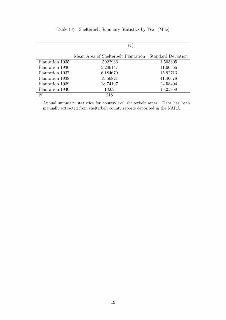
Table (3) Shelterbelt Summary Statistics by Year (Mile)

(1)

Mean Area of Shelterbelt Plantation Standard DeviationPlantation 1935 .5922936 1.503305Plantation 1936 5.286147 11.00566Plantation 1937 6.184679 15.92713Plantation 1938 19.56821 41.40678Plantation 1939 18.74197 24.58494Plantation 1940 13.09 15.25959N 218

Annual summary statistics for county-level shelterbelt areas. Data has beenmanually extracted from shelterbelt county reports deposited in the NARA.

19

Table (4) Effect of Commodity Price on Adoption

(1)VARIABLES Shelterbelt Acre

Initital Corn Intensity * Price -1.63e-06***(2.30e-07)

Initital Cotton Intensity * Price -8.14e-06***(9.88e-07)

Initital Wheat Intensity * Price -1.05e-06***(3.51e-07)

Constant 8.83e-05***(5.98e-06)

Observations 1,278Number of FIPS 217R-squared 0.137county FE YesYear FE Yes

Standard errors in parentheses*** p<0.01, ** p<0.05, * p<0.1

•Panel regression with five years of plantationdata for 217 counties in the Great Plains.This table follows regression model (1).

•Cotton, corn and wheat intensity have beenderived from 1930 USDA agricultural census.I use total farmland to get the intensity byarea.

• initial corn intensity*price denotes the in-teraction between initial corn intensity andcorn price movement of that year. initial cot-ton intensity*price denotes the interactionbetween initial cotton intensity and cottonprice movement of that year. initial wheat in-tensity*price denotes the interaction betweeninitial wheat intensity and wheat price move-ment of that year.

20

Table (5) Heerogeneous Treatment Effects of Commodity Price on Adoption

(1) (2) (3) (4) (5)VARIABLES Tenants Duration Irrigation Wood Num Farms

Price*Tenure*Cotton 2.51e-05**(1.26e-05)

Price*Tenure*Corn -1.09e-05***(3.61e-06)

Price*Tenure*Wheat 6.07e-06(5.37e-06)

Price*Duration*Cotton 7.59e-06(5.34e-06)

Price*Duration*Corn 2.21e-06*(1.14e-06)

Price*Duration*Wheat -9.36e-07(1.34e-06)

Price*Irrigation*Cotton 0.000189(0.000125)

Price*Irrigation*Corn 2.12e-05(3.20e-05)

Price*Irrigation*Wheat -0.000198**(8.07e-05)

Price*Wood*Cotton 3.31e-05***(1.20e-05)

Price*Wood*Corn 1.30e-05(1.48e-05)

Price*Wood*Wheat -4.50e-06(1.69e-05)

Price*Num Farm*Cotton -3.55e-10(1.05e-09)

Price*Num Farm*Corn 6.08e-10(3.81e-10)

Price*Num Farm*Wheat -6.58e-11(5.00e-10)

Constant 9.01e-05*** 8.99e-05*** 8.93e-05*** 8.77e-05*** 8.87e-05***(5.99e-06) (6.03e-06) (5.98e-06) (5.98e-06) (6.00e-06)

Observations 1,278 1,278 1,278 1,278 1,278R-squared 0.148 0.143 0.145 0.145 0.140Number of FIPS 217 217 217 217 217county FE Yes Yes Yes Yes YesYear FE Yes Yes Yes Yes Yes

Standard errors in parentheses*** p<0.01, ** p<0.05, * p<0.1

• Panel regression with five years of plantation data for 217 counties in the Great Plains. This tablefollows regression model (2).

• *Cotton, corn and wheat denotes initial crop intensity in 1930.

•Tenure denotes proportion of farms operated by tenants, Duration denotes average agriculturalcontract duration, irrigation denotes proportion of total farmland under irrigation, wood denotesproportion of pastureland under wood in 1934, Num Farm denotes total number of farms.

21

Table (6) Effect of Shelterbelt Adoption on Total Erosion

(1) (2) (3)first second

VARIABLES Total Rate Log Plantation Total Rate

Log Plantation 84.98 -258.0(198.9) (509.4)

Average size of farms, 1935 (acres) 0.000100 -7.03e-08**(0.000193) (3.18e-08)

Farms of black operators, 1935 (number) -0.000894 -2.88e-07(0.000582) (1.89e-07)

Tenants, 1935 (number) 1.04e-05 1.15e-08(8.20e-05) (2.57e-08)

treat IV 0.000130***(1.97e-05)

Constant 1.516*** 5.88e-05* 1.594***(0.126) (3.48e-05) (0.0709)

Observations 218 218 218R-squared 0.015 0.200

Robust standard errors in parentheses*** p<0.01, ** p<0.05, * p<0.1

Table 4 follows from regression model 3 and model 4. We use Total Plantation in 1930’sto explain the long-term persistent effect on total erosion in the shelterbelt counties. Wecontrol from average farm size, number of farms under black farmers, number of farmsunder tenant farms.treat˙IV is derived from the GPSP planning of 100 mile wide shelterbelt areas (Li, 2019).

22

Table (7) Effect of Plantation on Total Wind Erosion

(1) (2) (3)first second

VARIABLES Total Wind Rate Log Plantation Total Wind Rate

Log Plantation 514.4* -238.4(294.3) (762.6)

Average size of farms, 1935 (acres) 0.000480** -7.03e-08**(0.000237) (3.18e-08)

Farms of black operators, 1935 (number) -0.000420 -2.88e-07(0.000814) (1.89e-07)

Tenants, 1935 (number) -0.000213* 1.15e-08(0.000119) (2.57e-08)

treat IV 0.000130***(1.97e-05)

Constant 0.933*** 5.88e-05* 1.031***(0.173) (3.48e-05) (0.106)

Observations 218 218 218R-squared 0.100 0.200

Robust standard errors in parentheses*** p<0.01, ** p<0.05, * p<0.1

Table 5 follows from regression model 3 and model 4. We use Total Plantation in 1930’s to explain thelong-term persistent effect on total wind erosion in the shelterbelt counties. We control from averagefarm size, number of farms under black farmers, number of farms under tenant farms.treat˙IV is derived from the GPSP planning of 100 mile wide shelterbelt areas (Li, 2019).

23

Table (8) Effect of Plantation on total Pasture Erosion

(1) (2) (3)first second

VARIABLES Pasture Rate Log Plantation Pasture Rate

Log Plantation 72.97 -1,960***(217.0) (553.4)

Average size of farms, 1935 (acres) 0.000617** -7.52e-08*(0.000294) (3.91e-08)

Farms of black operators, 1935 (number) -0.000200 -2.85e-07(0.000319) (1.90e-07)

Tenants, 1935 (number) 4.89e-05 8.15e-09(8.13e-05) (2.65e-08)

treat IV 0.000131***(2.01e-05)

Constant 0.160 6.42e-05* 0.696***(0.169) (3.79e-05) (0.0780)

Observations 214 214 214R-squared 0.125 0.199

Robust standard errors in parentheses*** p<0.01, ** p<0.05, * p<0.1

*Table 6 follows from regression model 3 and model 4. We use Total Plantation in 1930’s toexplain the long-term persistent effect on total pastureland erosion in the shelterbelt counties.We control from average farm size, number of farms under black farmers, number of farms undertenant farms.treat˙IV is derived from the GPSP planning of 100 mile wide shelterbelt areas (Li, 2019).

24

Tab

le(9

)E

ffec

tof

Pla

nta

tion

onT

otal

Pas

ture

Win

dE

rosi

on

(1)

(2)

(3)

firs

tse

cond

VA

RIA

BL

ES

Pas

ture

Win

dR

ate

Log

Pla

nta

tion

Pas

ture

Win

dR

ate

Log

Pla

nta

tion

329.

8-1

,719

***

(224

.3)

(562

.6)

Ave

rage

size

offa

rms,

1935

(acr

es)

0.00

0747

**-7

.52e

-08*

(0.0

0036

3)(3

.91e

-08)

Far

ms

ofbla

ckop

erat

ors,

1935

(num

ber

)7.

67e-

05-2

.85e

-07

(0.0

0029

1)(1

.90e

-07)

Ten

ants

,19

35(n

um

ber

)1.

76e-

068.

15e-

09(9

.99e

-05)

(2.6

5e-0

8)tr

eat

IV0.

0001

31**

*(2

.01e

-05)

Con

stan

t-0

.099

16.

42e-

05*

0.45

3***

(0.2

13)

(3.7

9e-0

5)(0

.079

2)

Obse

rvat

ions

214

214

214

R-s

quar

ed0.

189

0.19

9R

obust

stan

dar

der

rors

inpar

enth

eses

***

p<

0.01

,**

p<

0.05

,*

p<

0.1

*T

ab

le7

foll

ows

from

regre

ssio

nm

odel

3an

dm

od

el4.

We

use

Tota

lP

lanta

tion

in1930’s

toex

pla

inth

elo

ng-t

erm

per

sist

ent

effec

ton

tota

lpast

ure

lan

dw

ind

erosi

on

inth

esh

elte

rbel

tco

unti

es.

We

contr

ol

from

aver

age

farm

size

,nu

mb

erof

farm

su

nder

bla

ckfa

rmer

s,nu

mb

erof

farm

su

nd

erte

nant

farm

s.tr

eat˙

IVis

der

ived

from

the

GP

SP

pla

nn

ing

of10

0m

ile

wid

esh

elte

rbel

tar

eas

(Li,

2019).

25

Tab

le(1

0)E

ffec

tof

Pla

nta

tion

onT

otal

Cro

pla

nd

Win

dE

rosi

on

(1)

(2)

(3)

firs

tse

cond

VA

RIA

BL

ES

Cro

pla

nd

Win

dR

ate

Log

Pla

nta

tion

Cro

pla

nd

Win

dR

ate

Log

Pla

nta

tion

769.

7**

66.8

3(3

42.4

)(8

29.3

)A

vera

gesi

zeof

farm

s,19

35(a

cres

)0.

0005

17**

-7.0

3e-0

8**

(0.0

0025

2)(3

.18e

-08)

Far

ms

ofbla

ckop

erat

ors,

1935

(num

ber

)-0

.000

322

-2.8

8e-0

7(0

.000

877)

(1.8

9e-0

7)T

enan

ts,

1935

(num

ber

)-0

.000

243*

1.15

e-08

(0.0

0012

8)(2

.57e

-08)

trea

tIV

0.00

0130

***

(1.9

7e-0

5)C

onst

ant

1.01

7***

5.88

e-05

*1.

100*

**(0

.186

)(3

.48e

-05)

(0.1

15)

Obse

rvat

ions

218

218

218

R-s

quar

ed0.

105

0.20

00.

002

Rob

ust

stan

dar

der

rors

inpar

enth

eses

***

p<

0.01

,**

p<

0.05

,*

p<

0.1

*Tab

le9

follow

sfr

omre

gres

sion

model

3an

dm

odel

4.W

euse

Tot

alP

lanta

tion

in19

30’s

toex

pla

inth

elo

ng-

term

per

sist

ent

effec

ton

tota

lcr

op

lan

dw

ind

erosi

on

inth

esh

elte

rbel

tco

unti

es.

We

contr

ol

from

aver

age

farm

size

,nu

mb

erof

farm

su

nd

erb

lack

farm

ers,

nu

mb

erof

farm

su

nd

erte

nan

tfa

rms.

trea

t˙IV

isd

eriv

edfr

omth

eG

PS

Pp

lan

nin

gof

100

mil

ew

ide

shel

terb

elt

area

s(L

i,20

19).

26

References

Adesina, Akinwumi A and Moses M Zinnah (1993). “Technology characteristics, farmers’

perceptions and adoption decisions: A Tobit model application in Sierra Leone”.

Agricultural economics 9.4, pp. 297–311.

Aigbokhaevbo, Violet O (2014). “The” Great Green Wall”: Implementation Constraints”.

Environmental Policy and Law 44.4, p. 375.

Alsan, Marcella and Claudia Goldin (2015). Watersheds in infant mortality: The role of

effective water and sewerage infrastructure, 1880 to 1915. Tech. rep. National Bureau

of Economic Research.

Beetz, Alice E (2011). Agroforestry: Overview. ATTRA.

Bellefontaine, Ronald, Martial Bernoux, Bernard Bonnet, Antoine Cornet, Christophe

Cudennec, Patrick D’Aquino, Isabelle Droy, Sandrine Jauffret, Maya Leroy, Michel

Malagnoux, et al. (2011). “The African great green wall project: What advice can

scientists provide?: A summary of published results”.

Brain, Stephen (2010). “The great Stalin plan for the transformation of nature”. Environ-

mental History 15.4, pp. 670–700.

Brown, Sarah E, Daniel C Miller, Pablo J Ordonez, and Kathy Baylis (2018). “Evidence for

the impacts of agroforestry on agricultural productivity, ecosystem services, and hu-

man well-being in high-income countries: a systematic map protocol”. Environmental

Evidence 7.1, p. 24.

Cassel, J Frank and John M Wiehe (1980). “Uses of shelterbelts by birds”. Workshop

Proceedings, Management of Western forests and Grasslands for Nongame Birds.

USDA Forest Service General Technical Report INT-86, Ogden, UT, pp. 78–87.

Cohen, Aaron J, Michael Brauer, Richard Burnett, H Ross Anderson, Joseph Frostad, Kara

Estep, Kalpana Balakrishnan, Bert Brunekreef, Lalit Dandona, Rakhi Dandona, et al.

(2017). “Estimates and 25-year trends of the global burden of disease attributable to

ambient air pollution: an analysis of data from the Global Burden of Diseases Study

2015”. The Lancet 389.10082, pp. 1907–1918.

27

Cowan, Tim, Sabine Undorf, Gabriele C Hegerl, Luke J Harrington, and Friederike EL

Otto (2020). “Present-day greenhouse gases could cause more frequent and longer

Dust Bowl heatwaves”. Nature Climate Change, pp. 1–6.

Droze, Wilmon Henry (1977). Trees, prairies, and people: a history of tree planting in the

plains states. Texas Woman’s University.

Elkin, Rosetta Sarah (2014). “Planting the Desert: Cultivating Green Wall Infrastructure”.

Revising Green Infrastructure. CRC Press, pp. 324–345.

Fishback, Price (2017). “How successful was the new deal? The microeconomic impact of

new deal spending and lending policies in the 1930s”. Journal of Economic Literature

55.4, pp. 1435–85.

Freire-Gonzalez, Jaume, Christopher Decker, and Jim W Hall (2017). “The economic

impacts of droughts: A framework for analysis”. Ecological Economics 132, pp. 196–

204.

Gardner, Robert (2009). “Trees as technology: planting shelterbelts on the Great Plains”.

History and technology 25.4, pp. 325–341.

Haines, Michael R et al. (2010). “Historical, demographic, economic, and social data: the

United States, 1790–2002”. Ann Arbor, MI: Inter-university Consortium for Political

and Social Research.

Hornbeck, Richard (2012). “The enduring impact of the American Dust Bowl: Short-

and long-run adjustments to environmental catastrophe”. The American Economic

Review 102.4, pp. 1477–1507.

Hornbeck, Richard and Pinar Keskin (2014). “The historically evolving impact of the

ogallala aquifer: Agricultural adaptation to groundwater and drought”. American

Economic Journal: Applied Economics 6.1, pp. 190–219.

Hornbeck, Richard and Suresh Naidu (2014). “When the levee breaks: black migration

and economic development in the American South”. American Economic Review

104.3, pp. 963–90.

Howlader, Aparna (2019). “Three essays on the relationship between land conservation

and economic development”. PhD thesis. University of Illinois at Urbana-Champaign.

28

Hughes, Karl, Seth Morgan, Katherine Baylis, Judith Oduol, Emilie Smith-Dumont, Tor-

Gunnar Vagen, and Hilda Kegode (2020). “Assessing the downstream socioeconomic

impacts of agroforestry in Kenya”. World Development 128, p. 104835.

Hurt, R Douglas (1981). The Dust Bowl: An agricultural and social history. Taylor Trade

Publications.

Jacks, DS (2017). Data on Real Commodity Prices, 1850—Present.

Li, Miao-miao, An-tian Liu, Chun-jing Zou, Wen-duo Xu, Hideyuki Shimizu, and Kai-yun

Wang (2012). “An overview of the “Three-North” Shelterbelt project in China”.

Forestry Studies in China 14.1, pp. 70–79.

Li, Tianshu (2019). “Protecting the Breadbasket with Trees? The Effect of the Great Plains

Shelterbelt Project on Agricultural Production”. American Journal of Agricultural

Economics RR.

McIntosh, C Barron (1975). “Use and abuse of the Timber Culture Act”. Annals of the

Association of American Geographers 65.3, pp. 347–362.

Meneguzzo, Dacia M, Andrew J Lister, and Cody Sullivan (2018). “Summary of findings

from the Great Plains Tree and Forest Invasives Initiative”. Gen. Tech. Rep. NRS-

GTR-177. Newtown Square, PA: US Department of Agriculture, Forest Service,

Northern Research Station. 24 p. 177, pp. 1–24.

Mercer, D Evan and Subhrendu K Pattanayak (2003). “Agroforestry adoption by small-

holders”. Forests in a market economy. Springer, pp. 283–299.

Miller, Daniel C, Pablo J Ordonez, Sarah E Brown, Samantha Forrest, Noe J Nava,

Karl Hughes, and Kathy Baylis (2020). “The impacts of agroforestry on agricultural

productivity, ecosystem services, and human well-being in low-and middle-income

countries: An evidence and gap map”. Campbell Systematic Reviews 16.1, e1066.

Munns, Edward N and Joseph H Stoeckeler (1946). “How are the great plains shelterbelts?”

Journal of Forestry 44.4, pp. 237–257.

Nair, PK Ramachandran (1993). An introduction to agroforestry. Springer Science &

Business Media.

29

Prokopy, Linda S, Kristin Floress, J Gordon Arbuckle, Sarah P Church, FR Eanes, Yuling

Gao, Benjamin M Gramig, Pranay Ranjan, and Ajay S Singh (2019). “Adoption of

agricultural conservation practices in the United States: Evidence from 35 years of

quantitative literature”. Journal of Soil and Water Conservation 74.5, pp. 520–534.

Read, Ralph A et al. (1958). “Great Plains shelterbelt in 1954”.

Reimer, Adam P, Ben M Gramig, and Linda S Prokopy (2013). “Farmers and conserva-

tion programs: explaining differences in Environmental Quality Incentives Program

applications between states”. Journal of Soil and Water Conservation 68.2, pp. 110–

119.

Rosenberg, Norman J (1986). “Adaptations to adversity: agriculture, climate and the

Great Plains of North America”. Great Plains Quarterly, pp. 202–217.

Scherr, Sara J (1992). “Not out of the woods yet: challenges for economics research on

agroforestry”. American journal of agricultural economics 74.3, pp. 802–808.

Schoeneberger, Michele M (2009). “Agroforestry: working trees for sequestering carbon

on agricultural lands”. Agroforestry systems 75.1, pp. 27–37.

Skidmore, EL and LJ Hagen (1977). “Reducing wind erosion with barriers”. Transactions

of the ASAE 20.5, pp. 911–0915.

Stein, John D and Patrick Charles Kennedy (1972). “Key to shelterbelt insects in the

Northern Great Plains”.

Stoeckeler, Joseph Henry et al. (1962). “Shelterbelt influence on Great Plains field

environment and crops”.

Woodruff, N P (1977). How to control wind erosion. 354. Dept. of Agriculture, Agricultural

Research Service: for sale by the Supt . . .

Young, Anthony et al. (1989). “Agroforestry for soil conservation”.

30