Detection of Metaldehyde in Water Using a LONESTARTM Portable

Analyzer

Contact us

www.owlstonenanotech.com

2 | P a g e

Contents

Introduction .................................................................................................................................... 3

The LONESTARTM Portable Analyzer ............................................................................................... 4

Experimental ................................................................................................................................... 5

Sample Preparation ........................................................................................................................ 7

Results ............................................................................................................................................. 8

Method Validation .......................................................................................................................... 9

Conclusion ..................................................................................................................................... 10

References .................................................................................................................................... 10

Appendix A: FAIMS Technology at a Glance ................................................................................. 11

Sample preparation and introduction ...................................................................................... 11

Carrier Gas ................................................................................................................................ 12

Ionisation Source ...................................................................................................................... 12

Mobility ..................................................................................................................................... 15

Detection and Identification ..................................................................................................... 16

3 | P a g e

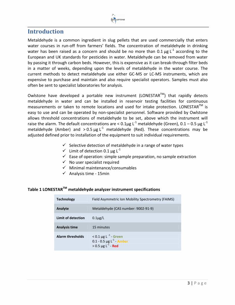
Introduction

Metaldehyde is a common ingredient in slug pellets that are used commercially that enters water courses in run-off from farmers’ fields. The concentration of metaldehyde in drinking water has been raised as a concern and should be no more than 0.1 µg L-1 according to the European and UK standards for pesticides in water. Metaldehyde can be removed from water by passing it through carbon beds. However, this is expensive as it can break-through filter beds in a matter of weeks, depending upon the levels of metaldehyde in the water course. The current methods to detect metaldehyde use either GC-MS or LC-MS instruments, which are expensive to purchase and maintain and also require specialist operators. Samples must also often be sent to specialist laboratories for analysis.

Owlstone have developed a portable new instrument (LONESTARTM) that rapidly detects metaldehyde in water and can be installed in reservoir testing facilities for continuous measurements or taken to remote locations and used for intake protection. LONESTARTM is easy to use and can be operated by non-specialist personnel. Software provided by Owlstone allows threshold concentrations of metaldehyde to be set, above which the instrument will raise the alarm. The default concentrations are < 0.1µg L-1 metaldehyde (Green), 0.1 – 0.5 µg L-1 metaldehyde (Amber) and > 0.5 µg L-1 metaldehyde (Red). These concentrations may be adjusted defined prior to installation of the equipment to suit individual requirements.

Selective detection of metaldehyde in a range of water types Limit of detection 0.1 µg L-1 Ease of operation: simple sample preparation, no sample extraction No user specialist required Minimal maintenance/consumables Analysis time - 15min

Table 1 LONESTARTM metaldehyde analyzer instrument specifications

Technology Field Asymmetric Ion Mobility Spectrometry (FAIMS)

Analyte Metaldehyde (CAS number: 9002-91-9)

Limit of detection 0.1µg/L

Analysis time 15 minutes

Alarm thresholds < 0.1 µg L -1

- Green 0.1 - 0.5 µg L

-1 - Amber

> 0.5 µg L-1

- Red

4 | P a g e

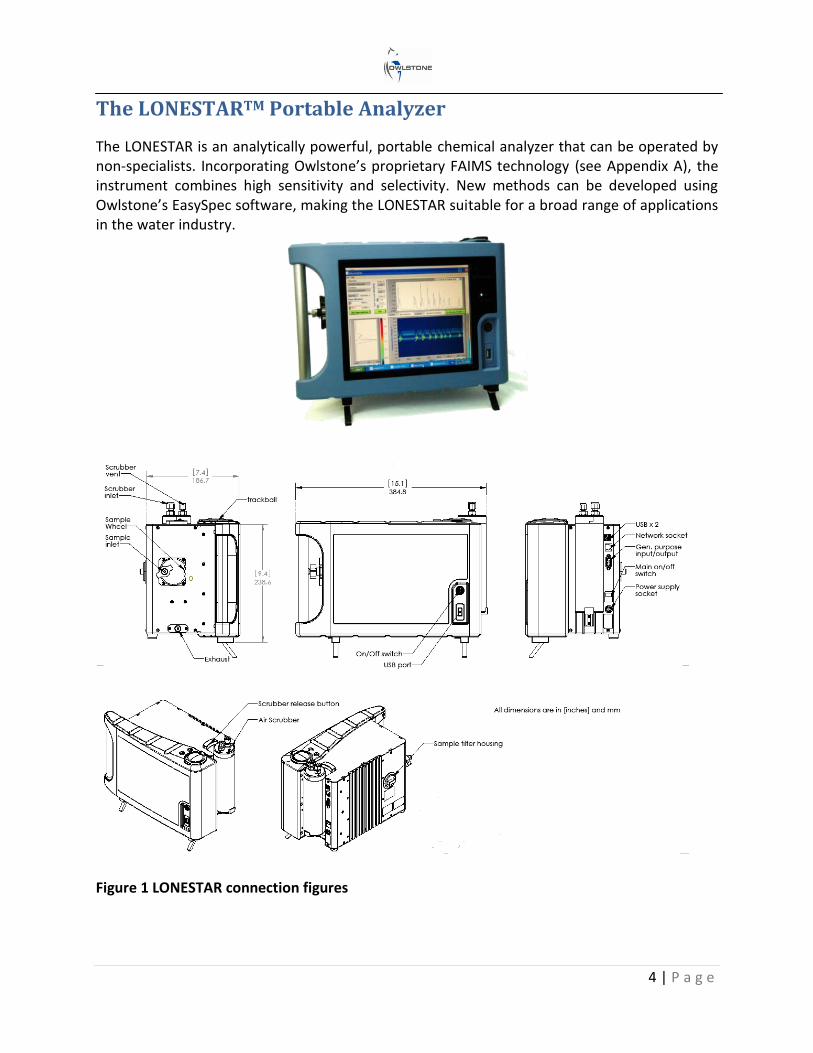
The LONESTARTM Portable Analyzer

The LONESTAR is an analytically powerful, portable chemical analyzer that can be operated by non-specialists. Incorporating Owlstone’s proprietary FAIMS technology (see Appendix A), the instrument combines high sensitivity and selectivity. New methods can be developed using Owlstone’s EasySpec software, making the LONESTAR suitable for a broad range of applications in the water industry.

Figure 1 LONESTAR connection figures

5 | P a g e

Experimental

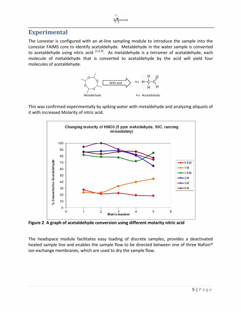
The Lonestar is configured with an at-line sampling module to introduce the sample into the Lonestar FAIMS core to identify acetaldehyde. Metaldehyde in the water sample is converted to acetaldehyde using nitric acid [1,2,3]. As metaldehyde is a tetramer of acetaldehyde, each molecule of metaldehyde that is converted to acetaldehyde by the acid will yield four molecules of acetaldehyde.

This was confirmed experimentally by spiking water with metaldehyde and analyzing aliquots of it with increased Molarity of nitric acid.

Figure 2 A graph of acetaldehyde conversion using different molarity nitric acid

The headspace module facilitates easy loading of discrete samples, provides a deactivated heated sample line and enables the sample flow to be directed between one of three Nafion® ion-exchange membranes, which are used to dry the sample flow.

6 | P a g e

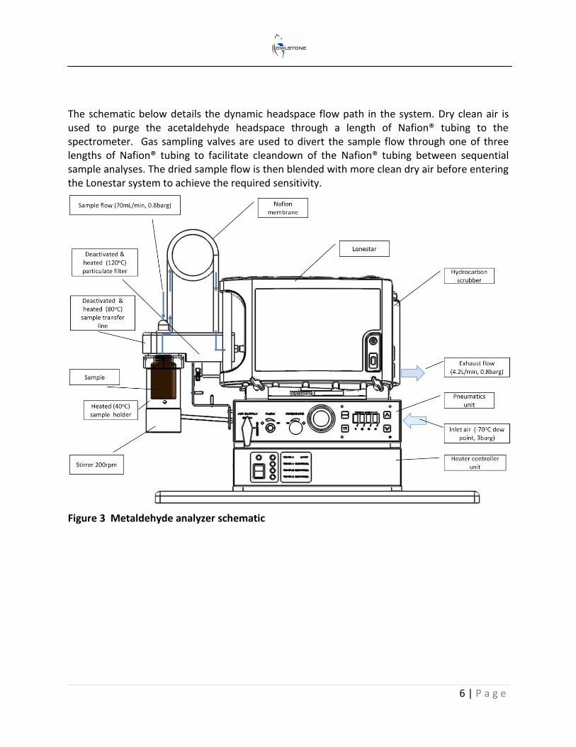
The schematic below details the dynamic headspace flow path in the system. Dry clean air is used to purge the acetaldehyde headspace through a length of Nafion® tubing to the spectrometer. Gas sampling valves are used to divert the sample flow through one of three lengths of Nafion® tubing to facilitate cleandown of the Nafion® tubing between sequential sample analyses. The dried sample flow is then blended with more clean dry air before entering the Lonestar system to achieve the required sensitivity.

Figure 3 Metaldehyde analyzer schematic

7 | P a g e

Sample Preparation

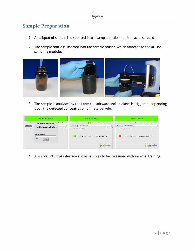
1. An aliquot of sample is dispensed into a sample bottle and nitric acid is added.

2. The sample bottle is inserted into the sample holder, which attaches to the at-line

sampling module.

3. The sample is analysed by the Lonestar software and an alarm is triggered, depending upon the detected concentration of metaldehyde.

4. A simple, intuitive interface allows samples to be measured with minimal training.

8 | P a g e

Results

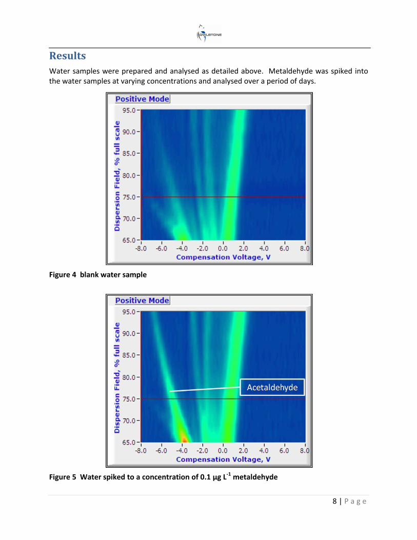
Water samples were prepared and analysed as detailed above. Metaldehyde was spiked into the water samples at varying concentrations and analysed over a period of days.

Figure 4 blank water sample

Figure 5 Water spiked to a concentration of 0.1 µg L-1 metaldehyde

9 | P a g e

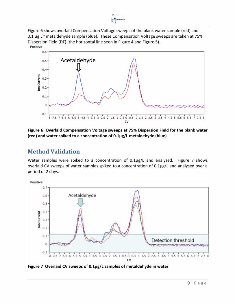
Figure 6 shows overlaid Compensation Voltage sweeps of the blank water sample (red) and 0.1 µg L-1 metaldehyde sample (blue). These Compensation Voltage sweeps are taken at 75% Dispersion Field (DF) (the horizontal line seen in Figure 4 and Figure 5).

Figure 6 Overlaid Compensation Voltage sweeps at 75% Dispersion Field for the blank water (red) and water spiked to a concentration of 0.1µg/L metaldehyde (blue)

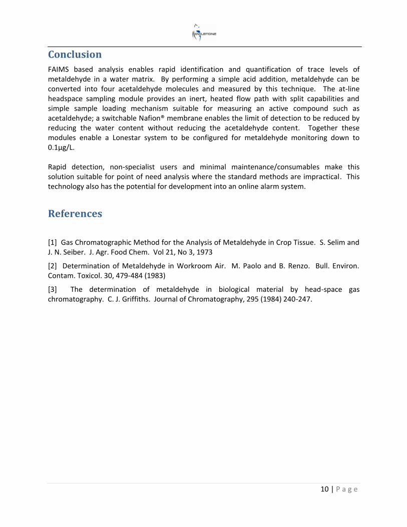
Method Validation

Water samples were spiked to a concentration of 0.1µg/L and analysed. Figure 7 shows overlaid CV sweeps of water samples spiked to a concentration of 0.1µg/L and analysed over a period of 2 days.

Figure 7 Overlaid CV sweeps of 0.1µg/L samples of metaldehyde in water

10 | P a g e

Conclusion

FAIMS based analysis enables rapid identification and quantification of trace levels of metaldehyde in a water matrix. By performing a simple acid addition, metaldehyde can be converted into four acetaldehyde molecules and measured by this technique. The at-line headspace sampling module provides an inert, heated flow path with split capabilities and simple sample loading mechanism suitable for measuring an active compound such as acetaldehyde; a switchable Nafion® membrane enables the limit of detection to be reduced by reducing the water content without reducing the acetaldehyde content. Together these modules enable a Lonestar system to be configured for metaldehyde monitoring down to 0.1µg/L. Rapid detection, non-specialist users and minimal maintenance/consumables make this solution suitable for point of need analysis where the standard methods are impractical. This technology also has the potential for development into an online alarm system.

References

[1] Gas Chromatographic Method for the Analysis of Metaldehyde in Crop Tissue. S. Selim and J. N. Seiber. J. Agr. Food Chem. Vol 21, No 3, 1973

[2] Determination of Metaldehyde in Workroom Air. M. Paolo and B. Renzo. Bull. Environ. Contam. Toxicol. 30, 479-484 (1983)

[3] The determination of metaldehyde in biological material by head-space gas chromatography. C. J. Griffiths. Journal of Chromatography, 295 (1984) 240-247.

11 | P a g e

Appendix A: FAIMS Technology at a Glance

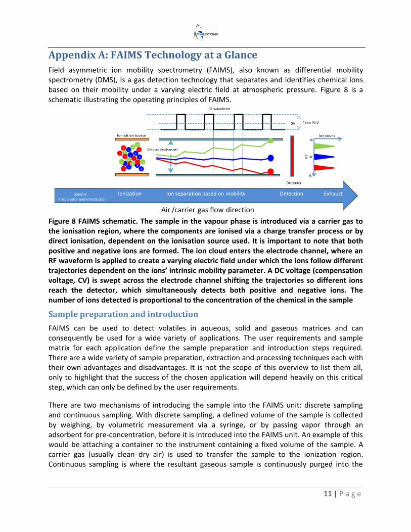
Field asymmetric ion mobility spectrometry (FAIMS), also known as differential mobility spectrometry (DMS), is a gas detection technology that separates and identifies chemical ions based on their mobility under a varying electric field at atmospheric pressure. Figure 8 is a schematic illustrating the operating principles of FAIMS.

Figure 8 FAIMS schematic. The sample in the vapour phase is introduced via a carrier gas to the ionisation region, where the components are ionised via a charge transfer process or by direct ionisation, dependent on the ionisation source used. It is important to note that both positive and negative ions are formed. The ion cloud enters the electrode channel, where an RF waveform is applied to create a varying electric field under which the ions follow different trajectories dependent on the ions’ intrinsic mobility parameter. A DC voltage (compensation voltage, CV) is swept across the electrode channel shifting the trajectories so different ions reach the detector, which simultaneously detects both positive and negative ions. The number of ions detected is proportional to the concentration of the chemical in the sample

Sample preparation and introduction

FAIMS can be used to detect volatiles in aqueous, solid and gaseous matrices and can consequently be used for a wide variety of applications. The user requirements and sample matrix for each application define the sample preparation and introduction steps required. There are a wide variety of sample preparation, extraction and processing techniques each with their own advantages and disadvantages. It is not the scope of this overview to list them all, only to highlight that the success of the chosen application will depend heavily on this critical step, which can only be defined by the user requirements.

There are two mechanisms of introducing the sample into the FAIMS unit: discrete sampling and continuous sampling. With discrete sampling, a defined volume of the sample is collected by weighing, by volumetric measurement via a syringe, or by passing vapor through an adsorbent for pre-concentration, before it is introduced into the FAIMS unit. An example of this would be attaching a container to the instrument containing a fixed volume of the sample. A carrier gas (usually clean dry air) is used to transfer the sample to the ionization region. Continuous sampling is where the resultant gaseous sample is continuously purged into the

-6+

60

Ionisation source

-

-

+

+

+ -

+ +

-

-

-

+

-

-

+

+

+ -

++

-

--

+

CV

Detector

Electrode channel

RF waveform

Air /carrier gas flow direction

Pk to Pk V 0V

Sample Ionization Ion separation based on mobility Detection ExhaustPreparation and introduction

Ion count

12 | P a g e

FAIMS unit and either is diluted by the carrier gas or acts as the carrier gas itself. For example, continuously drawing air from the top of a process vat.

The one key requirement for all the sample preparation and introduction techniques is the ability to reproducibly generate and introduce a headspace (vapour) concentration of the target analytes that exceeds the lower limits of detection of the FAIMS device.

Carrier Gas

The requirement for a flow of air through the system is twofold: Firstly to drive the ions through the electrode channel to the detector plate and secondly, to initiate the ionization process necessary for detection. As exhibited in Figure 9, the transmission factor (proportion of ions that make it to the detector) increases with increasing flow. The higher the transmission factor, the higher the sensitivity. Higher flow gives a larger full width half maximum (FWHM) of the peaks but also decreases the resolution of the FAIMS unit (see Figure 10). The air/carrier gas determines the baseline reading of the instrument. Therefore, for optimal operation it is desirable for the carrier to be free of all impurities (< 0.1 ppm methane) and the humidity to be kept constant. It can be supplied either from a pump or compressor, allowing for negative and positive pressure operating modes.

Ionisation Source

There are three main vapor phase ion sources in use for atmospheric pressure ionization; radioactive nickel-63 (Ni-63), corona discharge (CD) and ultra-violet radiation (UV). A comparison of ionization sources is presented in Table 2.

Ionisation Source Mechanism Chemical Selectivity

Ni63

(beta emitter) creates a positive / negative RIP Charge transfer Proton / electron affinity

UV (Photons) Direct ionisation First ionisation potential

Corona discharge (plasma) creates a positive / negative RIP

Charge transfer Proton / electron affinity

Table 2 FAIMS ionization source comparison

Figure 9 Flow rate vs. ion transmission factor

Figure 10 FWHM of ion species at set CV

13 | P a g e

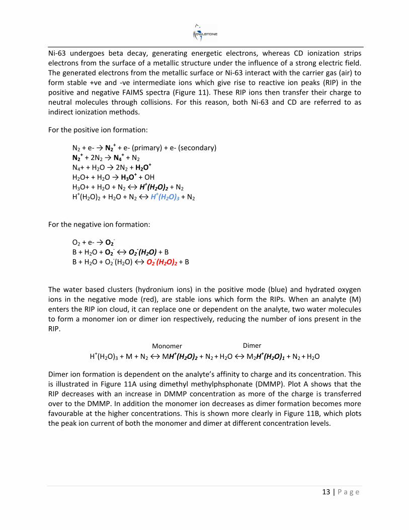
Ni-63 undergoes beta decay, generating energetic electrons, whereas CD ionization strips electrons from the surface of a metallic structure under the influence of a strong electric field. The generated electrons from the metallic surface or Ni-63 interact with the carrier gas (air) to form stable +ve and -ve intermediate ions which give rise to reactive ion peaks (RIP) in the positive and negative FAIMS spectra (Figure 11). These RIP ions then transfer their charge to neutral molecules through collisions. For this reason, both Ni-63 and CD are referred to as indirect ionization methods.

For the positive ion formation:

N2 + e- → N2+ + e- (primary) + e- (secondary)

N2+ + 2N2 → N4

+ + N2 N4+ + H2O → 2N2 + H2O+ H2O+ + H2O → H3O+ + OH H3O+ + H2O + N2 ↔ H+(H2O)2 + N2 H+(H2O)2 + H2O + N2 ↔ H+(H2O)3 + N2

For the negative ion formation:

O2 + e- → O2-

B + H2O + O2- ↔ O2

-(H2O) + B B + H2O + O2

-(H2O) ↔ O2-(H2O)2 + B

The water based clusters (hydronium ions) in the positive mode (blue) and hydrated oxygen ions in the negative mode (red), are stable ions which form the RIPs. When an analyte (M) enters the RIP ion cloud, it can replace one or dependent on the analyte, two water molecules to form a monomer ion or dimer ion respectively, reducing the number of ions present in the RIP.

H+(H2O)3 + M + N2 ↔ MH+(H2O)2 + N2 + H2O ↔ M2H

+(H2O)1 + N2 + H2O

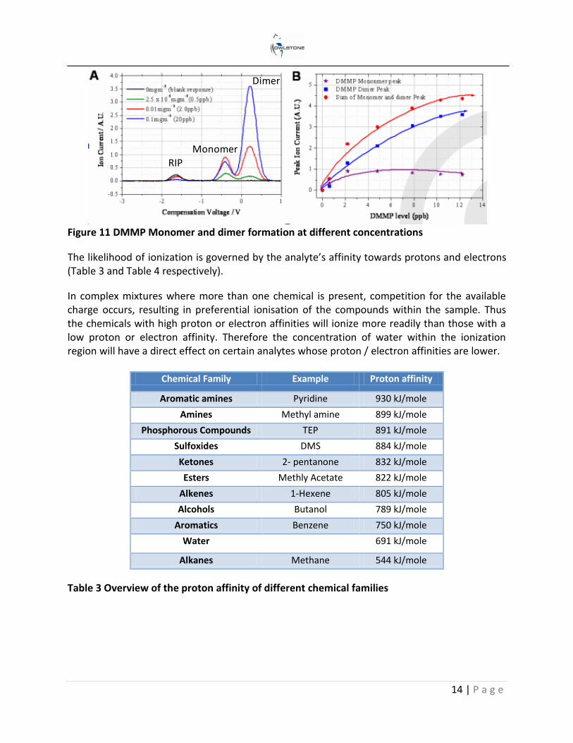
Dimer ion formation is dependent on the analyte’s affinity to charge and its concentration. This is illustrated in Figure 11A using dimethyl methylphsphonate (DMMP). Plot A shows that the RIP decreases with an increase in DMMP concentration as more of the charge is transferred over to the DMMP. In addition the monomer ion decreases as dimer formation becomes more favourable at the higher concentrations. This is shown more clearly in Figure 11B, which plots the peak ion current of both the monomer and dimer at different concentration levels.

Monomer Dimer

14 | P a g e

Figure 11 DMMP Monomer and dimer formation at different concentrations

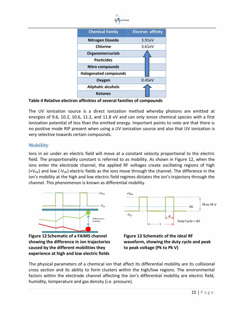
The likelihood of ionization is governed by the analyte’s affinity towards protons and electrons (Table 3 and Table 4 respectively).

In complex mixtures where more than one chemical is present, competition for the available charge occurs, resulting in preferential ionisation of the compounds within the sample. Thus the chemicals with high proton or electron affinities will ionize more readily than those with a low proton or electron affinity. Therefore the concentration of water within the ionization region will have a direct effect on certain analytes whose proton / electron affinities are lower.

Chemical Family Example Proton affinity

Aromatic amines Pyridine 930 kJ/mole

Amines Methyl amine 899 kJ/mole

Phosphorous Compounds TEP 891 kJ/mole

Sulfoxides DMS 884 kJ/mole

Ketones 2- pentanone 832 kJ/mole

Esters Methly Acetate 822 kJ/mole

Alkenes 1-Hexene 805 kJ/mole

Alcohols Butanol 789 kJ/mole

Aromatics Benzene 750 kJ/mole

Water 691 kJ/mole

Alkanes Methane 544 kJ/mole

Table 3 Overview of the proton affinity of different chemical families

RIP

Monomer

Dimer

15 | P a g e

Chemical Family Electron affinity

Nitrogen Dioxide 3.91eV

Chlorine 3.61eV

Organomercurials

Pesticides

Nitro compounds

Halogenated compounds

Oxygen 0.45eV

Aliphatic alcohols

Ketones

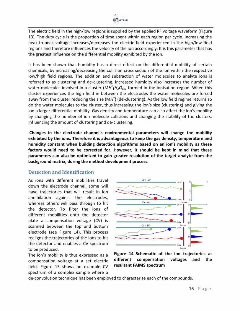
Table 4 Relative electron affinities of several families of compounds

The UV ionization source is a direct ionization method whereby photons are emitted at energies of 9.6, 10.2, 10.6, 11.2, and 11.8 eV and can only ionize chemical species with a first ionization potential of less than the emitted energy. Important points to note are that there is no positive mode RIP present when using a UV ionization source and also that UV ionization is very selective towards certain compounds.

Mobility

Ions in air under an electric field will move at a constant velocity proportional to the electric field. The proportionality constant is referred to as mobility. As shown in Figure 12, when the ions enter the electrode channel, the applied RF voltages create oscillating regions of high (+VHF) and low (-VHF) electric fields as the ions move through the channel. The difference in the ion’s mobility at the high and low electric field regimes dictates the ion’s trajectory through the channel. This phenomenon is known as differential mobility.

Figure 12 Schematic of a FAIMS channel showing the difference in ion trajectories caused by the different mobilities they experience at high and low electric fields

Figure 13 Schematic of the ideal RF waveform, showing the duty cycle and peak to peak voltage (Pk to Pk V)

The physical parameters of a chemical ion that affect its differential mobility are its collisional cross section and its ability to form clusters within the high/low regions. The environmental factors within the electrode channel affecting the ion’s differential mobility are electric field, humidity, temperature and gas density (i.e. pressure).

-VLF

+VHF

Difference in mobility

Pk to Pk V 0V

+VHF

-VLF d

Duty Cycle = d/t t

16 | P a g e

The electric field in the high/low regions is supplied by the applied RF voltage waveform (Figure 13). The duty cycle is the proportion of time spent within each region per cycle. Increasing the peak-to-peak voltage increases/decreases the electric field experienced in the high/low field regions and therefore influences the velocity of the ion accordingly. It is this parameter that has the greatest influence on the differential mobility exhibited by the ion.

It has been shown that humidity has a direct effect on the differential mobility of certain chemicals, by increasing/decreasing the collision cross section of the ion within the respective low/high field regions. The addition and subtraction of water molecules to analyte ions is referred to as clustering and de-clustering. Increased humidity also increases the number of water molecules involved in a cluster (MH+(H2O)2) formed in the ionisation region. When this cluster experiences the high field in between the electrodes the water molecules are forced away from the cluster reducing the size (MH+) (de-clustering). As the low field regime returns so do the water molecules to the cluster, thus increasing the ion’s size (clustering) and giving the ion a larger differential mobility. Gas density and temperature can also affect the ion’s mobility by changing the number of ion-molecule collisions and changing the stability of the clusters, influencing the amount of clustering and de-clustering.

Changes in the electrode channel’s environmental parameters will change the mobility exhibited by the ions. Therefore it is advantageous to keep the gas density, temperature and humidity constant when building detection algorithms based on an ion’s mobility as these factors would need to be corrected for. However, it should be kept in mind that these parameters can also be optimized to gain greater resolution of the target analyte from the background matrix, during the method development process.

Detection and Identification

As ions with different mobilities travel down the electrode channel, some will have trajectories that will result in ion annihilation against the electrodes, whereas others will pass through to hit the detector. To filter the ions of different mobilities onto the detector plate a compensation voltage (CV) is scanned between the top and bottom electrode (see Figure 14). This process realigns the trajectories of the ions to hit the detector and enables a CV spectrum to be produced. The ion’s mobility is thus expressed as a compensation voltage at a set electric field. Figure 15 shows an example CV spectrum of a complex sample where a de-convolution technique has been employed to characterize each of the compounds.

Figure 14 Schematic of the ion trajectories at different compensation voltages and the resultant FAIMS spectrum

CV -6V

Detector

CV 6V

-6

V+6V

-0V

CV -6V

Detector

CV 6V

-6

V+6

V-

0V

CV-6V

Detector

CV 6V

-6V+6

V-0V

CV = -5V

CV = 0V

CV = 5V

17 | P a g e

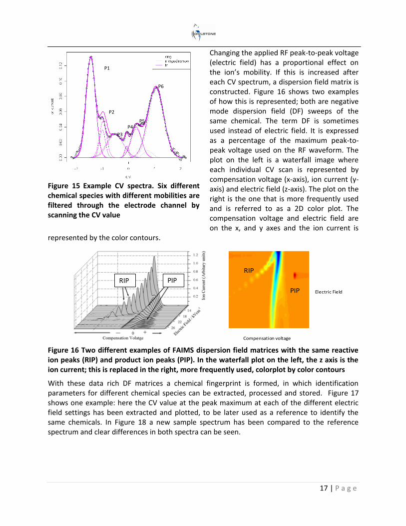
Changing the applied RF peak-to-peak voltage (electric field) has a proportional effect on the ion’s mobility. If this is increased after each CV spectrum, a dispersion field matrix is constructed. Figure 16 shows two examples of how this is represented; both are negative mode dispersion field (DF) sweeps of the same chemical. The term DF is sometimes used instead of electric field. It is expressed as a percentage of the maximum peak-to-peak voltage used on the RF waveform. The plot on the left is a waterfall image where each individual CV scan is represented by compensation voltage (x-axis), ion current (y-axis) and electric field (z-axis). The plot on the right is the one that is more frequently used and is referred to as a 2D color plot. The compensation voltage and electric field are on the x, and y axes and the ion current is

represented by the color contours.

Figure 16 Two different examples of FAIMS dispersion field matrices with the same reactive ion peaks (RIP) and product ion peaks (PIP). In the waterfall plot on the left, the z axis is the ion current; this is replaced in the right, more frequently used, colorplot by color contours

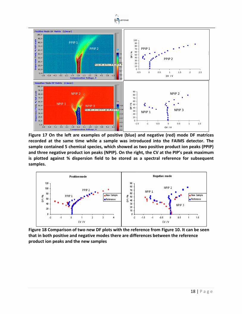
With these data rich DF matrices a chemical fingerprint is formed, in which identification parameters for different chemical species can be extracted, processed and stored. Figure 17 shows one example: here the CV value at the peak maximum at each of the different electric field settings has been extracted and plotted, to be later used as a reference to identify the same chemicals. In Figure 18 a new sample spectrum has been compared to the reference spectrum and clear differences in both spectra can be seen.

PIPRIP

Figure 15 Example CV spectra. Six different chemical species with different mobilities are filtered through the electrode channel by scanning the CV value

Electric Field

Compensation voltage

PIP

RIP

P1

P2

P3

P4 P5

P6

18 | P a g e

Figure 17 On the left are examples of positive (blue) and negative (red) mode DF matrices recorded at the same time while a sample was introduced into the FAIMS detector. The sample contained 5 chemical species, which showed as two positive product ion peaks (PPIP) and three negative product ion peaks (NPIP). On the right, the CV at the PIP’s peak maximum is plotted against % dispersion field to be stored as a spectral reference for subsequent samples.

Figure 18 Comparison of two new DF plots with the reference from Figure 10. It can be seen that in both positive and negative modes there are differences between the reference product ion peaks and the new samples

0

10

20

30

40

50

60

70

80

90

100

-0.5 0 0.5 1 1.5 2 2.5

CV / V

DF

/ % Pork at 7 Days

0

10

20

30

40

50

60

70

80

90

-1.5 -1 -0.5 0 0.5 1 1.5

CV / V

DF

/ % Pork at 7 Days

PPIP 1

PPIP 2

NPIP 1

NPIP 2

NPIP 3

PPIP 1

PPIP 2

NPIP 1

NPIP 2

NPIP 3