detection of citrus canker using hyperspectral...
TRANSCRIPT

1
DETECTION OF CITRUS CANKER USING HYPERSPECTRAL IMAGING TECHNIQUE
By
NIKHIL PRAMOD NIPHADKAR
A THESIS PRESENTED TO THE GRADUATE SCHOOL OF THE UNIVERSITY OF FLORIDA IN PARTIAL FULFILLMENT
OF THE REQUIREMENTS FOR THE DEGREE OF MASTER OF SCIENCE
UNIVERSITY OF FLORIDA
2010

2
© 2010 Nikhil Pramod Niphadkar

3
To my Aai and Baba
And
To all my Gurus
|| Gururbramha gururvishnu gururdevo maheshwara ||
|| Guru sakshyat parabramha tasmaishri guruve namaha ||

4
ACKNOWLEDGMENTS
I would like to thank my advisor Dr. Thomas F. Burks for providing me a priceless
guidance and encouragement during the course of this research. I am also grateful to
Dr. Wonsuk Lee and Dr. Clint Slatton for the invaluable technical assistance they
provided by being on my thesis committee. I would also like to thank Dr. Warren Dixon
for being my advisor in Mechanical and Aerospace Engineering department.
In addition, I would like to appreciate the valued support provided by my
colleagues Dr. Jianwei Qin and Dr. Duke Bulanon, without whose help this research
could not have completed. Also, I would like to express my gratitude to Mr. Mike Zingaro
and Mr. Greg Pugh for their precious help in building the hyperspectral imaging system
and all the technical aid they provided. At last but not the least, I would like to thank all
my friends for being there during the hard times and encouraging me to keep going.

5
TABLE OF CONTENTS Page
ACKNOWLEDGMENTS .................................................................................................. 4
LIST OF TABLES ............................................................................................................ 9
LIST OF FIGURES ........................................................................................................ 10
ABSTRACT ................................................................................................................... 12
1 INTRODUCTION .................................................................................................... 15
Overview of United States Citrus Industry .............................................................. 15 Necessity of the Automated Detection System ....................................................... 16
2 OBJECTIVES OF RESEARCH ............................................................................... 19
Estimation of Detection Limit for Size of Citrus Canker Lesions Based on Hyperspectral Imaging ......................................................................................... 19
Detection of Citrus Canker Using RGB Color Image Along with Near Infrared (NIR) Monochrome Images ................................................................................. 19
Compensation of Edge Effect on Spherical Objects due to Light Source – Hyperspectral Imaging Application ...................................................................... 20
3 LITERATURE REVIEW .......................................................................................... 21
Citrus Canker .......................................................................................................... 22 Image Processing Techniques Used in Agriculture ................................................ 23 Hyperspectral and Multispectral Imaging Based Approaches Used in Agriculture .. 29 Hyperspectral and Multispectral Imaging Coupled with Computer Vision and
Pattern Classification Approaches ....................................................................... 32
4 OVERVIEW OF MATERIALS AND METHODS ...................................................... 35
Citrus Samples ....................................................................................................... 35 Hyperspectral Imaging System ............................................................................... 37 Image Pre-Processing ............................................................................................ 38 Flat field correction ................................................................................................. 39 Image Masking and Binning .................................................................................... 41 Hyperspectral Band Selection Using Correlation Analysis (CA) ............................. 41 Image Classification ................................................................................................ 43 Principle Component Analysis (PCA) ..................................................................... 44 Estimation of Detection Limit for Size of Citrus Canker Lesions Based on
Hyperspectral Imaging ......................................................................................... 45

6
Detection of Citrus Canker Using RGB Color Image Along with NIR Monochrome Images ........................................................................................... 46
Compensation of Edge Effect on Spherical Objects due to Light Source – Hyperspectral Imaging Application ...................................................................... 47
5 ESTIMATION OF DETECTION LIMIT FOR SIZE OF CITRUS CANKER LESIONS BASED ON HYPERSPECTRAL REFLECTANCE IMAGING ................. 51
Introduction ............................................................................................................. 51 Materials and Methods............................................................................................ 54
Citrus Samples ................................................................................................. 54 Hyperspectral Imaging System ......................................................................... 55 Image Pre-Processing ...................................................................................... 57 Hyperspectral Band Selection .......................................................................... 58 Image Classification ......................................................................................... 59 Binary Lesion Size Detection Algorithm ........................................................... 60 Mapping Binary Lesion Size to Original Hyperspectral Image .......................... 61
Results, Observations and Discussion.................................................................... 62 Image Classification Results ............................................................................ 62 Binary Lesion Size Estimation Results ............................................................. 63 Results of Mapping Binary Lesion Size to Original Hyperspectral Image ......... 64
Summary and Conclusion ....................................................................................... 66
6 DETECTION OF CITRUS CANKER USING RGB COLOR IMAGE ALONG WITH NEAR-INFRARED MONOCHROME IMAGES ............................................. 76
Introduction ............................................................................................................. 76 Materials and Methods............................................................................................ 79
Citrus Samples ................................................................................................. 79 Hyperspectral Imaging System ......................................................................... 80 Image Pre-Processing ...................................................................................... 82 Simulation of RGB Color Image ....................................................................... 82 Combining RGB Color Image and Remaining Monochrome Images ............... 83 Hyperspectral Band Selection .......................................................................... 84 Image Classification ......................................................................................... 86
Results, Observations and Discussion.................................................................... 87 Key Wavelengths for Canker Detection ............................................................ 87 Ratio Images .................................................................................................... 89 Image Classification Results ............................................................................ 89 Why RGB Image Can’t Be Used for Canker Identification? .............................. 92
Summary and Conclusion ....................................................................................... 97
7
7 COMPENSATION OF EDGE EFFECT ON IMAGES OF SPHERICAL OBJECTS DUE TO LIGHT SOURCE – HYPERSPECTRAL IMAGING APPLICATION ...................................................................................................... 107
Introduction ........................................................................................................... 107 Materials and Methods.......................................................................................... 110
Hyperspectral Imaging System ....................................................................... 110 Flat Field Correction ....................................................................................... 112 Image Masking and Binning ........................................................................... 114 Derivation of Geometric Correction Factor ..................................................... 114 Generating the Digital Elevation Model .......................................................... 118 Estimation of Geometric Correction Factors ................................................... 122 Algorithm Validation Tests .............................................................................. 123
Results, Observations and Discussion.................................................................. 125 Digital Elevation Model Observations ............................................................. 125 Geometric Correction Factor Observations and Results ................................ 126 Validation Test Results ................................................................................... 127
Summary and Conclusion ..................................................................................... 130
8 OVERALL SUMMARY, CONCLUSIONS AND FUTURE SCOPE ........................ 141
Summary and Conclusions ................................................................................... 141 Future Scope ........................................................................................................ 143
APPENDIX
A MATLAB CODE FILES - ESTIMATION OF DETECTION LIMIT FOR SIZE OF CITRUS CANKER LESIONS BASED ON HYPERSPECTRAL REFLECTANCE IMAGING .............................................................................................................. 145
B MATLAB CODE FILES - DETECTION OF CITRUS CANKER USING RGB COLOR IMAGE ALONG WITH NIR MONOCHROME IMAGES ........................... 147
Main Program File ................................................................................................ 147 Simulation of the RGB + NIR images ............................................................. 147 Generation of Spectra of Different Disease Conditions .................................. 149
Function Files ....................................................................................................... 150 Function to Perform the Correlation Analysis on the Image Data ................... 150 Function to Read the Image File in ENVI Format in MATLAB ........................ 152 Function to Write the MATLAB Array into an Image File in ENVI Format ....... 154
C MATLAB CODE FILES - COMPENSATION OF EDGE EFFECT ON IMAGES OF SPHERICAL OBJECTS DUE TO LIGHT SOURCE ........................................ 156
Main Program File ................................................................................................ 156 Function Files ....................................................................................................... 160

8
LIST OF REFERENCES ............................................................................................. 162
BIOGRAPHICAL SKETCH .......................................................................................... 166

9
LIST OF TABLES
Table Page 4-1 Numbers of fruit samples for each peel condition ............................................... 50
5-1 Numbers of fruit samples for each peel condition ............................................... 74
5-2 Summary of classification results ....................................................................... 74
5-3 Effect of number of erosion cycles on canker lesion size estimation .................. 75
6-1 Summary of classification results ..................................................................... 106

10
LIST OF FIGURES
Figure Page 4-1 Representative normal and diseased peel conditions of grapefruit samples ...... 48
4-2 Hyperspectral imaging system for reflectance image acquisition from grapefruits........................................................................................................... 49
4-3 Image classification procedure ........................................................................... 50
5-1 Representative normal and diseased peel conditions of grapefruit samples ...... 68
5-2 Hyperspectral imaging system for reflectance image acquisition from grapefruits........................................................................................................... 69
5-3 Image Classification Procedure .......................................................................... 70
5-4 Classification Method-Discrimination of canker from other peel conditions ........ 71
5-5 Effect of variation of threshold values on classification accuracies..................... 72
5-6 Final Binary Image of a sample before and after applying the ‘bwareaopen’ function ............................................................................................................... 72
5-7 Mapping binary lesion size to original hyperspectral image ................................ 73
5-8 Probability distribution of lesion size of all samples ............................................ 73
5-9 Probability distribution of lesion size of subset of all samples ............................ 74
6-1 Representative normal and diseased peel conditions of grapefruit samples ...... 99
6-2 Hyperspectral imaging system for reflectance image acquisition from grapefruits......................................................................................................... 100
6-3 Red, Green and Blue filter transmittance characteristics .................................. 101
6-4 Contour of correlation coefficients between two band ratios and fruit peel conditions ......................................................................................................... 102
6-5 Mean reflectance spectra of grapefruits with different peel conditions ............. 103
6-6 Two band Ratio images for different disease conditions. (From L to R Canker, Greasy Spot, Insect Damage, Normal, Melanose, Scab, Wind Scar) . 103
6-7 Image classification procedure ......................................................................... 104

11
6-8 Values of two band ratio between 771 and 739 nm (R771/R739) for different peel conditions .................................................................................................. 105
6-9 Effect of variation of threshold values on classification accuracies................... 105
7-1 Hyperspectral imaging system for reflectance image acquisition from grapefruits......................................................................................................... 132
7-2 Pilot points and center of mass ......................................................................... 133
7-3 Pilot points (red in color) and nodes of interpolation (green in color) of one of the meridians .................................................................................................... 133
7-4 Transversal plane formed by maximum fruit height (hc) and center of mass of the fruit (Cg). The computed elevations of the interpolation nodes is also shown by ‘center line’ ....................................................................................... 134
7-5 Side view of the modeled ellipse and the elevations of interpolation nodes ..... 135
7-6 3-D view of the modeled ellipse and the elevations of interpolation nodes ....... 135
7-7 Digital elevation model ..................................................................................... 136
7-8 Contour of geometric correction factor (εg) ....................................................... 137
7-9 Effect of application of geometric correction – Single band image at 724 nm .. 137
7-10 Citrus sample marked with the angular graduations and the regions of interest .............................................................................................................. 138
7-11 Reflectance spectra of ROI 3............................................................................ 139
7-12 Reflectance spectra of all three ROIs at the rotation of 40 degrees ................. 140

12
Abstract of Thesis Presented to the Graduate School of the University of Florida in Partial Fulfillment of the Requirements for the Degree of Master of Science
DETECTION OF CITRUS CANKER USING HYPERSPECTRAL IMAGING
TECHNIQUE
By
Nikhil Pramod Niphadkar
May 2010
Chair: Thomas F Burks Major: Agricultural and Biological Engineering
The citrus industry of Florida has led the economy of the State of Florida to
prosperity. The statistics shows that Florida produces maximum citrus supply
throughout United States. However, one of the biggest challenges the industry has been
facing for quite a while is citrus canker. The reason citrus canker being such an
important issue is its fast spread and very high damage potential which is affecting the
export of citrus fruits to several international markets including European countries.
Presently the stress is on preventing the cankerous citrus fruits from entering the
unaffected regions. The studies have proven that the automated detection systems can
help in prevention of citrus canker and thus reduce the serious loss Florida citrus
industry has been facing. The basic underlying objective of this thesis was to develop
an approach for canker detection for a real time application on a packaging line using
hyperspectral imaging. The thesis consisted of three different studies, the outcomes of
which are abstracted here.
The first study was aimed at estimating the capability of the previously developed
multispectral algorithm using correlation analysis to detect smallest possible canker
lesion on the citrus fruit. More specifically the goal of this work was to determine the

13
size of the smallest canker lesion that can be detected. The optimal wavelengths
selected using correlation analysis were 834 nm and 729 nm. The best overall
classification accuracy achieved was 95.7% when the binary threshold value of 1.275
was used. This threshold value was found to give best tradeoff between canker
classification and overall classification. The smallest lesion detected by the lesion size
estimation algorithm had the surface area of 2.16 sq. mm. and equivalent diameter was
1.66 mm.
The second part of the thesis consisted of an attempt to develop a novel approach
to discriminate citrus canker from other surface conditions. The idea was to explore if a
two camera system with one CCD color camera (to capture RGB color image) and one
monochrome camera (to capture NIR single band image) could be built for canker
detection in online real time packaging application. As this was an experimental study,
the hybrid hyperspectral image including RGB color image and NIR single band images
was simulated using previously captured hyperspectral image data (450 - 930 nm). This
image was then subjected to the correlation analysis (CA) to identify the key channels.
The CA did not select any of the red, green or blue channels as significant channels for
canker identification. The reason being higher bandwidths of the R, G and B channels
which not only might have included the information to detect canker but also other peel
conditions. It was concluded that RGB color image (along with some single band
monochrome image) cannot be utilized to discriminate canker from other peel
conditions based on simple thresholding technique.
The third and final piece of the thesis was to re-implement the compensation
algorithm to eliminate the adverse effects of light source while capturing the image of

14
spherical objects like citrus fruits. The motivation behind this study was to reduce the
misclassification of citrus fruits due to the edge blackening effect which our research
team had been facing. The algorithm was developed by Gomez et al. 2007. The image
was corrected for the spatial variations (flat field correction) caused by intensity of light
source as well as geometrical variation caused by the spherical geometry of the citrus
fruit. The geometric correction was accomplished by constructing a 3-D digital elevation
model (DEM) of the fruit from its 2-D image. This DEM provided us with the geometric
properties of the fruit like X, Y, and Z coordinates which were exploited in the course of
estimating the geometric correction factor for each pixel. The corrected image portrayed
improved and uniform brightness of the citrus fruit surface throughout. Few tests were
also conducted to validate the results of the algorithm which essentially proved that the
geometric correction results in uniform intensity of radiation throughout the fruit surface.
15
CHAPTER 1 INTRODUCTION
Citrus production is the second largest industry in the State of Florida. More than
70% of the citrus supply of United States is produced in Florida. Citrus industry has
proved to be an important source of employment to many. The agricultural economy
and the economy in general of the State of Florida is influenced significantly by the
citrus industry. And hence one can safely say that to improve the economy of the state
we should target the citrus and various related industries.
However, the Florida citrus industry has been facing a serious challenge of
disease control. Among different diseases, citrus canker has proven to be one of the
most devastating diseases that endanger the marketability of the citrus crops. Citrus
canker can infect most commercial citrus varieties. Caused by bacterial pathogen
Xanthomonas axonopodis, the disease is characterized by conspicuous, erumpent
lesions on leaves, stems, and fruit. Citrus canker could cause defoliation, blemished
fruit, premature fruit drop, twig dieback, and tree decline. Due to its fast spread, high
damage potential, and massive impact on export and domestic trade, canker is
considered as one of the most disturbing diseases that threaten all citrus-growing areas.
The emphasis of this particular exploration is on developing the measures that could
differentiate between diseased and marketable citrus fruits, preventing them from
entering the canker free areas and thereby restricting the further spread of the disease.
Overview of United States Citrus Industry
Florida leads U.S. citrus production and accounts for a major part of the U.S. citrus
industry. According to the citrus production report (USDA, 2005-06), Florida accounts
for more than 70% of U.S. citrus production. Florida produces a number of different

16
citrus products. Orange, grapefruit, and lemons are major citrus crops, with lesser
production in tangerines, limes, and an increasing variety of specialties. Oranges
account for more than 80 percent (Hodge et al., 2001). Orange and grapefruit account
for about 90 percent of U.S. production (Jacobs et al., 1994). Florida, California/Arizona,
and Texas are the major states for U.S. citrus productions. Florida accounted for more
than three quarters of all U.S. citrus, while California/Arizona and Texas had the
remainder. Citrus is consumed not only as fresh fruit but also in products that use citrus
fruits. Florida has 52 citrus processing plants (Hodges et al., 2001). They produce
various orange juice items such as chilled, canned juice, and concentrated juice. These
plants also produce many byproducts like citrus pulp, molasses, and the essential
oil-limonene (Hodges et al., 2001) along with a number of byproducts like food
additives, cattle feed, and cosmetics.
Necessity of the Automated Detection System
Twenty first century is characterized by technological advances. Automated
systems are used everywhere. Various scientists, organizations etc. have been working
hard to bring automation into the agricultural industry. Since the citrus production
volume in Florida is very large, it is really difficult to inspect all the fruits using human
inspectors. Also, after a while, human inspectors are prone to make mistakes because
of the fatigue caused by repetition. Moreover in the packaging industries, the conveyors
are designed to carry the fruits at considerably high speeds (say 5 to 10 fruits per
second). At such high speeds, it becomes almost impossible for the human inspectors
to catch the diseased fruits. In such cases, automated disease detection systems prove
to be the ultimate solution, the performance of which does not get affected by long
working hours. The automated systems hence not only improve the performance of the

17
detection but they also reduce the labor expenses needed otherwise. The hyperspectral
imaging has provided a new facet to the automated disease detection systems. This
particular thesis consists of three basic components:
1. Estimation of detection limit for size of citrus canker lesions based on hyperspectral imaging
2. Detection of citrus canker using RGB color image along with NIR monochrome images
3. Compensation of edge effect on spherical objects due to light source – Hyperspectral imaging application
The first part aims at estimating smallest possible canker lesion that can be
detected using the hyperspectral imaging technique. The misclassification of cankerous
citrus fruits with very small canker lesions was the motivating factor behind this
exploration. The previously developed multispectral algorithm using hyperspectral
wavelengths by our research group was used for segregation of cankerous citrus fruits
from fruits with other peel conditions (normal, greasy spot, insect damage, melanose,
scab and wind scar). We then used the image processing techniques such as
morphological opening to estimate the size of smallest lesion detected.
The second part of this thesis is dedicated to development of an innovative
algorithm for classification of citrus fruits into diseased and marketable class. There are
totally seven classes, six diseases (canker, greasy spot, insect damage, melanose,
scab, windscar) and a marketable class. The algorithm makes use of visible and Near
Infrared (NIR) wavelengths of hyperspectral image as separate channels lumped
together to create a single image. The resulting image is then processed further using
some multivariate statistical algorithms like principle component analysis (PCA) or
correlation analysis (CA) to identify the key wavelengths in the NIR region which will

18
help separate the cankerous citrus fruit from fruits of other peel conditions. The basic
objective behind this was to simulate the output of the two camera system installed on
the packaging line, including one CCD camera (outputting the RGB image) and one
monochrome camera (outputting the single NIR wavelength image) to provide four
channels of red, green, blue and NIR wavelength which in turn would be used to detect
canker. The motivation behind this research was, RGB images have proven to be a
good source to detect the physical defects like bruises on biological products while NIR
wavelengths have shown a good potential to detect canker on citrus fruits (Qin et al.,
2008 and 2009). In addition sooty mold which typically gets confused with other disease
symptom can be detected at 510 nm which is already covered in the RGB region. So
combining these two regions (RGB and NIR) can provide a means to identify all types of
defects that can be found on citrus fruits in a very cost effective manner.
When a computer vision system is used to capture the image of a spherical object,
the curvature of the object results in some adverse effects like darkening of the edges.
This darkening of edges may misguide the algorithm to detect a normal peel as
damaged or diseased. This was the underlying inspiration for re-implementing the edge
effect compensation algorithm developed by Gomez-Sanchis et al., (2007) which
constitutes the third and final part of the thesis. A correction factor was calculated for
every fruit pixel by generating the 3-D model of the fruit called digital elevation model
(DEM) and obtaining geometric properties like Cartesian coordinates for each pixel.
Application of this correction to the fruit image resulted in uniform intensity over the fruit
surface reducing the edge darkening.

19
CHAPTER 2 OBJECTIVES OF RESEARCH
This thesis constitutes of three major components. The objectives of each of them
are mentioned below:
Estimation of Detection Limit for Size of Citrus Canker Lesions Based on Hyperspectral Imaging
The main objective of this exploration was to estimate the detection limit for the
size of citrus canker lesions. Following were the sub-objectives to achieve the final goal:
• To use the previously developed multispectral algorithm for detecting the smallest possible cankerous lesion on the citrus fruit.
• To determine the controlling factors and their optimal values in canker lesion size estimation.
Detection of Citrus Canker Using RGB Color Image Along with Near Infrared (NIR) Monochrome Images
The main aim was to develop an algorithm to classify citrus fruits in diseased and
marketable classes. The intermediary objectives were:
• To simulate the grayscale images of “Red”, “Green” and “Blue” channels of the citrus fruit from the already available 3-D hyperspectral image dataset.
• To combine the “Red”, “Green” and “Blue” channels along with the rest of monochrome images (wavelengths not considered in creating the RGB image i.e., 700 to 930 nm) from the hyperspectral data.
• Select the appropriate channels/wavelengths using PCA or CA for canker classification.
• To simulate the output of a two camera system providing a single image containing the RGB image along with the selected NIR monochrome image.

20
Compensation of Edge Effect on Spherical Objects due to Light Source – Hyperspectral Imaging Application
To implement the algorithm to determine the compensation factor for the images
of citrus fruits to reduce the blackening effect at the edges of the fruit, was the lead goal
of this study which was achieved with the help of the following intermediate goals:
• To correct the images for the spatial variations of light source using a flat white panel of known reflectance
• To produce a 3-D model (digital elevation model-DEM) of the citrus fruit by assuming it to be Lambertian ellipsoidal surface from its 2-D image
• To derive the geometric correction to correct the images for edge effect using the geometric properties (Cartesian coordinates) of the fruit obtained from the DEM
• To validate that the images of citrus fruits corrected using the estimated compensation factor have similar reflectance throughout the fruit surface, minimizing the edge blackening effect.

21
CHAPTER 3 LITERATURE REVIEW
The citrus industry plays a very crucial role in improving the economy of the State
of Florida. Being the growers of world class citrus fruits, Florida farmers are very
concerned about not only the quality but also the cost effectiveness of the citrus
production. The citrus groves are usually spread over large acreages and hence it
demands significant labor to manage the groves and to control the pests. Also this is a
very time consuming and expensive job which needs to be done periodically. Apart from
all this, as the citrus fruits are produced in large quantity and they need to be inspected
for diseases which is also labor intensive and costly. Hence the citrus growers are
intending to use some automation application to assist managing their citrus groves and
the crops more economically.
There are two types of such automation applications usually found in agricultural
industry; one type is used for infield applications and other for indoor, packaging
applications. As most of these applications make use of some kind of machine vision,
image acquisition and processing technique, most of the infield applications are
influenced more by the intensity of light and ambient conditions than that of the indoor
applications. In recent studies, researchers have exploited computer vision techniques
coupled with pattern classification algorithms for agricultural applications such as
disease and defect detection, segregation of fruits and vegetables, identifying fruits in
the tree canopy, etc. This chapter is dedicated to introduction of the previous research
in the field of agriculture based machine vision applications. We will start with the
background information of one of the most serious diseases which Florida citrus
industry is facing.

22
Citrus Canker
The geographical origin of citrus canker is a matter of controversy. However
researchers have suggested that canker might have initiated in the tropical regions of
Asia i.e., South China, Indonasia, India, etc., where the citrus species are presumed to
be originated (Schubert et al., 2001; Das 2003). Citrus canker has spread all over the
world and is now in more than thirty countries in Asia, the Pacific and Indian Ocean
Islands, South America and Southern-Eastern USA. Some areas of the world (e.g.,
South Africa, Australia, the Fiji Islands, Mozambique, and New Zealand) have
eradicated citrus canker completely. However active ongoing eradication programs still
continue in other infected areas such as Argentina, Uruguay, Brazil, and Florida
(Schubert et al., 2001). It should be noted that in recent years, Florida has abandoned
the eradication program since the disease has become endemic.
Citrus canker usually occurs in regions with warm, humid and cloudy climate. This
disease is primarily caused by the bacterium named Xanthomonas axonopodis pv. citri.
Citrus canker was first found Florida around 1912 and then it spread all over the state in
the last few decades. The Citrus Canker Eradication Program (CCEP), initiated by the
Florida Department of Agriculture and Consumer Services - Division of Plant Industry
(FDACS-DPI) and the United States Department of Agriculture - Animal and Plant
Health Inspection Service (USDA-APHIS) in mid 1990’s, was an attempt to alleviate the
consequences that canker would have on the Florida citrus industry, as well as to keep
other U.S. citrus-producing areas (e.g., Texas and California) from being infected and
harmed by this disease. Because canker exhibits endemic features in most infected
regions, there is no universal treatment or prevention that could completely eradicate
the disease in all the infected areas. The current emphasis is put on minimizing the level

23
of the disease and preventing its further spread to the areas that are unaffected or were
already eradicated. The presence of cankerous fruit in a shipment could result in the
whole shipment being deemed unmarketable to some ‘canker-free’ areas, such as the
European countries.
Citrus canker is characterized by several symptoms on tree leaves, stems and
fruits. The symptoms on leaves at initial stage include slightly raised tiny blister-like
lesions which at later stage turn tan to brown. The center of the lesion becomes raised
and corky. The lesions are usually visible on both sides of the leaf. Symptoms on twigs
and fruit are similar and consisted of dark brown or black raised corky lesions
surrounded by an oily or water-soaked margin. As the lesions mature, they appear
scabby or corky. Lesions cause blemishes and early fruit drop, and hence results in
reduced fruit yield. Defoliation, premature fruit drop, twig dieback, general tree decline,
and very bad blemishes on fruit are the results of severe infestation. The canker
infected trees become weak, unproductive, and unprofitable. The cankerous citrus fruits
are unacceptable to the market but as canker is not harmful to human beings the juice
market does not get affected because of canker. Citrus canker is extremely infectious
and can be spread rapidly by wind-driven rain, storm events such as tornadoes and
tropical storms, flooding, equipment, and human movement within groves (Zekri et al.,
2005).
Image Processing Techniques Used in Agriculture
Burks et al. (2000) used the color co-occurrence method (CCM) and neural
network for classifying weed species. They extracted a total of 33 features using CCM
which were analyzed using SAS discriminant procedure STEPDISC. They reported poor
classification performance for feature models consisting only hue features or only

24
saturation features. The neural network with back-propagation demonstrated the
capability for identification of weed species with classification rates as high as 96.7%.
The individual species were also classified with classification accuracies of 90.0%.
Pydipati et al. (2006) also used the color co-occurrence method (CCM) to analyze
if it is possible to identify diseased and normal citrus leaves using texture based hue,
saturation and intensity (HSI) color features along with statistical classification
algorithms like SAS STEPDISC, under laboratory conditions. They created three CCM
matrices, one each for H, S and I, using spatial grey level dependence matrices
(SGDM’s) which then were used to generate the texture features. A total of 39 features
(13 each for H, S and I) were generated. The SAS statistical analysis using procedure
called STEPDISC was conducted to reduce redundancy in texture feature set and to
create different data models. The leaf sample discriminant analysis using CCM textural
features achieved classification accuracies of over 95% for all diseases when using hue
and saturation texture features. Classification models based on intensity features alone,
resulted in a reduction in classification accuracy when analyzing leaf fronts, due to the
darker pigmentation of the leaf fronts unlike the leaf backs where the lighter
pigmentation clearly revealed the disease discoloration. The overall best performance
was determined with a reduced data model that relied on hue and saturation features
only even if high accuracies were achieved when using an unreduced dataset
consisting of all HSI texture features. This model was selected due to reduced
computational load and the elimination of intensity features, which were not robust in
the presence of ambient light variation. From the study of Burks et al. (2000) and

25
Pydipati et al. (2006), it can be concluded that if only hue, only saturation or only
intensity features are used alone for classification, the classifier perform poorly.
Pydipiti et al. (2005) also tried to apply pattern recognition algorithms like statistical
and neural network classifiers for detection of diseases on citrus leaves. The 39 texture
features were generated (using SGDM’s) from the citrus leaf samples and redundancy
in the texture features was reduced (using SAS STEPDISC) in a similar way to form
different data models. In this study they analyzed only backs of the leaves. They applied
the following real time classifiers to all the data models and computed the classification
accuracies for each of them: 1) statistical classifier using Mahalanobis minimum
distance method 2) neural network with back propagation, and 3) neural network with
radial basis functions. They used the preliminary classification results of “generalized
square distance classifier” (which is a non real time classification approach) as the
bench mark for comparing the above real time classification approaches. The
Mahalanobis minimum distance classifier gave the overall classification accuracy of
98%, where those for neural network with back propagation and neural network with
radial basis functions were 98% and 95%, respectively. All the three classifier agreed
that the reduced feature set including hue and saturation features gave the best results
due to absence of intensity features, as intensity features may vary a lot in the outdoor
lighting conditions.
Park and Chen (2000) studied the texture features of co-occurrence matrix related
to distance and direction of neighborhood matrix and wavelength of multispectral
images of chicken carcasses to identify the important texture features along with the
important wavelengths to classify the carcasses into wholesome and unwholesome

26
classes. They concluded that variance, sum average, sum variance and sum entropy
were the most significant features to identify the unwholesome carcasses while angular
second moment was important to differentiate wholesome carcasses at both visible an
NIR wavelengths. They could discriminate the unwholesome chicken carcasses with the
accuracy of 95.6% using the linear discriminant model with covariance matrix analysis
while the accuracy of detection of wholesome carcasses was 97.0% using the quadratic
discriminant model with covariance matrix analysis. Both the linear and quadratic
models utilized the co-occurrence texture features of spectral images at visible and NIR
wavelengths, however the above mentioned optimum accuracies were obtained when
spectral image at 570 nm wavelength was used as input to the model.
Recently, Kim et al. (2009) also demonstrated that color imaging and texture
feature analysis could be used for differentiating citrus peel diseases under laboratory
conditions. Essentially they also followed a similar procedure that was followed by other
researchers in this type of study. They developed a color imaging system to acquire the
RGB color images from grapefruits. All the captured images were then analyzed using
the color co-occurrence method (CCM). To reduce the amount of data for processing a
small region of interest (ROI) was selected from each image. These ROIs were then
subjected to RGB to HSI (hue, saturation and intensity) domain conversion. To facilitate
the use of color co-occurrence method the spatial gray-level dependence matrices
(SGDMs) were generated. Total three SGDMs per ROI image were generated. These
SGDMs were then used to compute different texture features. 13 texture features per
SGDM per image were computed totaling 39 texture features for every image. The
appropriate texture features were selected out of those 39 using the stepwise

27
discrimination procedure by SAS called STEPDISC in order to reduce the redundancy
in the texture feature set. They developed four classification models using the SAS
procedure called DISCRIM. Out of those four models, HSI_13 which had total 13 texture
features from hue, saturation and intensity color space, acquired the best classification
results with overall classification accuracy of 96.7%. They also checked the stability of
this model which showed that the average classification accuracy for 10 different runs of
the model was 96.0% with a standard deviation of 2.3%, which proved that the model
HSI_13 is quite stable and could be successfully used for differentiating cankerous
citrus peel from other disease conditions under laboratory environment.
Whenever a computer vision system is used to capture images of spherical
objects, due to curvature of the object the edges of the objects appear darker than the
center. In such cases there is a possibility of these darker areas at the edge being
misclassified as diseased by the segregation algorithm (which is used for separation
diseased and healthy products). Gomez et al. (2007) presented an algorithm to correct
these adverse effects due to curvature of the spherical objects. They modeled the fruit
as Lambertian ellipsoidal surface (whose characteristic property is that it reflects light in
exactly the same way in all directions regardless of the direction from which it is
observed) and created a 3-D model (digital elevation model-DEM) of the fruit from the
2-D image mask of the fruit. This 3-D model – DEM was used to determine the
geometric correction factor for each of the pixel of the image. The value of this
correction factor was dependant on the location of the pixel. The corrected image had a
similar reflectance throughout its surface. This was validated by conducting numerous

28
experiments which essentially proved that after geometric correction the intensity of
radiation becomes uniform over the fruit surface.
Unay and Gosselin (2006) applied the various pattern recognition techniques to
identify stem and calyx of apples. They used high resolution digital monochrome
camera with four filters centered at 450, 500, 750 and 800 nm with bandwidths 80, 40,
80 and 50 nm, respectively. The method included the following steps: background
removal, object segmentation, feature extraction, feature selection, and pattern
classification. The image at 750 nm was used for segmentation which segmented the
objects by adaptive thresholding. A total of 35 features were extracted for each
segmented object. To eliminate the redundant features, sequential floating forward
selection (SFFS) method was used. The method selected 9 useful features out of 35
discarding the rest. They tried five different pattern recognition algorithms (linear
discriminant classifier, nearest neighbor, fuzzy nearest neighbor, support vector
machine and adaboost) and compared their performances. They found the support
vector machine to achieve best classification accuracies of 99% for stems and 100% for
calyxes using selected feature set. Also 13% of defects on the apple skin were
misclassified as stem or calyx. They concluded that along with low contrast and partial
segmentation due to erosion if the stem or calyx is located far from the center closer to
the edge in the image then it had a higher probability of getting misclassified the reason
being the captured images of the spherical object appear darker at edges than center.
This observation was found in line with that found by Gomez et al. (2007) during his
invention of edge effect compensation algorithm.

29
Hyperspectral and Multispectral Imaging Based Approaches Used in Agriculture
In the recent years, hyperspectral and multispectral imaging techniques have been
developed as useful tools for quality and safety evaluation of food and agricultural
products. The hyperspectral imaging technique acquires spatial information across a
sequence of individual band in a broad wavelength range, which generates a 3-D image
cube with a high spectral resolution. Kim et al. (2001) of the United States Department
of Agriculture (USDA) demonstrated such potential with the sample fluorescence and
reflectance images of normal apple and an apple with fungal contamination and bruised
spots captured using a laboratory based hyperspectral imaging system. He also
suggested that such a unique system can also be used for numerous scientific
applications.
Qin et al. (2008) analyzed the reflectance images of Ruby Red Grape fruits in the
wavelength range of 400-900 nm captured with the help of the portable hyperspectral
imaging system for classifying them into marketable and six diseased peel conditions
(canker, greasy spot, insect damage, melanose, scab, and windscar). These images
were then processed using principle component analysis (PCA) to compress the 3-D
hyperspectral image data into useful image features which could then be used to
separate cankerous samples from other diseased and marketable peel conditions. The
maximum overall canker detection accuracy was of the order of 93.0%. They identified
four wavelengths (553, 677, 718, and 858 nm) which could be adopted by the future
online real time solution for detecting canker on the sorting machine in packaging
industry.
Piron et al. (2007) worked towards determining the optimal combination of
wavelength filters for detecting various weed species located within the carrot rows in

30
the field. An infield multispectral imaging device consisting of a black and white camera
coupled with a rotating wheel holding 22 interference filters in VIS-NIR region was used
for the study. The quadratic discriminant analysis was used to determine the finest filter
combination. The best filter combination selected was 450, 550 and 700 nm which
accomplished the overall classification accuracy of 72.0%. They reported better
classification rates with an advanced stage of growth.
Although plenty spectral information is fairly useful for laboratory research, the 3-D
hyperspectral image cube contains lot of redundant information across wavelength
range being captured. Consequently, real-time hyperspectral image acquisition and
processing is challenging due to the large amount of data. Hence Lee et al. (2008)
made use of correlation analysis (CA) to select multispectral wavelengths from the 3-D
hyperspectral image data for defect detection on apples. The VIS-NIR reflectance
spectra extracted from the hyperspectral images of apples were used to identify the
wavelength pair for detecting the defect regions on apple surface. Such an optimal pair
of wavelengths was selected with the help of correlation analysis between band ratio
(λ1/λ2) or band difference (λ1-λ2) and the assigned value for the surface condition (0 =
normal or 1 = defect). The best wavelengths obtained with band ratio were 670 and 684
nm while those obtained with band difference were 828 and 734 nm which gave the
correlation coefficients of 0.91 and 0.79, respectively. The maximum overall
classification accuracy obtained was 92.42% (195 out of 211 defects).
A similar study was conducted by Qin et al. (2009) for detecting canker on citrus
fruits. He developed a multispectral method to inspect citrus canker based on band
selection from the hyperspectral images. He used both the correlation analysis (CA) and

31
principle component analysis (PCA) for the band selection and then compared the
results of both. He selected two bands using CA (band ratio), and three & four bands
using sequential forward CA (band ratio) and two bands using PCA. The overall
classification accuracy of two band ratio classifier using correlation analysis (95.7%)
was found to be better than that (92.8%) of the two band ratio classifier using principle
component analysis. The three and four band ratio classifiers using CA did not perform
(94.2% and 93.3%, respectively) as well as two band ratio classifier using CA which
suggests that adding more bands in image ratio calculations does not necessarily
improve the canker detection accuracy.
Kim et al. (2007) presented a single hyperspectral line scan imaging inspection
system with multi-tasking capabilities to detect not only the defects and diseases on the
apples but also the fecal contamination on the apples for online real time application. To
detect the fecal contamination the fluorescence imaging was used while the defects
were identified using reflectance imaging. The fluorescence imaging using band ratio of
F660/F530 (fluorescence at particular wavelengths) achieved 100.0% segregation of
feces contaminated apples from the non-contaminated ones (irrespective of diseased or
healthy). The reflectance imaging using band ratio of R800/R750 (reflectance at
particular wavelengths) coupled with SAS discriminant analysis could reach the
classification accuracies of 98.0% for healthy apples and 99.4% for defective apples. He
is in the process of evaluating the online system to simultaneously acquire the above
multispectral reflectance and fluorescence images. He claimed that it is possible to
configure the vision system to capture only a few selected spectral channels to speed
up the classification rate. Preset rate of detection is three apples / sec; however he is

32
modifying the hardware and software to improve the detection rate to more than 10
apples / sec. The basic aim of the exploration was to invent an inspection system with
multi-tasking capabilities with presently available infrastructure which he seemed to
achieve.
Lu (2002) investigated the use of near infrared (NIR) hyperspectral imaging for
detection of bruises on apples. His aim was to find out the spectral range and spectral
resolution along with development of an algorithm for effective detection of bruises of
different stages on different variety of apples (red delicious and golden delicious). He
made used of principle component analysis (PCA) coupled with minimum noise fraction
transform (MNF) to identify the bruises. He concluded that the spectral range of 1000
nm to 1340 nm with resolution 17.3 nm and 8.6 nm is best suitable for bruise detection
on all the variety of apples considered for the study. The best possible correct
classification rate for red delicious apples was 88.0% while the worst possible incorrect
classification rate was 12.0%. These numbers for golden delicious apples were 94.0%
(correct classification) and 7.0% (incorrect classification). He also proposed that with the
improved speed of image acquisition and improved detector technology, NIR
hyperspectral imaging can be a solution for offline inspection and online sorting of fruit
defects.
Hyperspectral and Multispectral Imaging Coupled with Computer Vision and Pattern Classification Approaches
Cheng at al. (2004) presented a new approach which combined the principle
component analysis (PCA) along with Fisher’s linear discriminant (FLD) to generate the
hybrid PCA-FLD method for maximizing the representation and classification effects on
the extracted new feature bands (wavelengths). PCA uses orthogonal axes for
33
dimensionality reduction by performing the eigen decomposition of the data co-variance
matrix. However, it is not necessarily good at drawing distinction between patterns,
being an unsupervised method. On the other hand FLD makes the data more reliable
for classification by projecting the scatter of the data but it is noise sensitive and may
not convey enough energy from original data. The hybrid PCA-FLD method maximizes
the advantages of the two methods and compensates for the disadvantages by
introducing a weighting factor in the computation. He used the hybrid method along with
individual methods PCA and FLD to discriminate the damaged (because of excessive
chilling) cucumbers from the good ones and finally compared the results to prove that
the hybrid PCA-FLD method outperforms the individual PCA and FLD methods.
Aleixos et al. (2001) developed a multispectral system to identify the size, color
(ripe or unripe) and skin defects on the citrus fruits using digital signal processors and
machine vision techniques. The system was developed for commercial fruit sorting and
packaging house for real time classification of fruits based on size, shape, color and
defects. The vision system consisted of two cameras, one CCD camera to capture the
RGB image while other monochrome camera with an infrared filter centered at 750 nm
to capture the infrared band. The infrared band (I) image alone was used to detect the
size and shape of the fruit (by applying a simple threshold to segment the fruit from
background) while all the R, G, B and I bands were used to detect the color and the
surface defects. Two separate DSP’s workings in parallel were used to detect the size &
shape and color & defects at the same time to minimize the processing time. The color
detection was performed with an accuracy of more than 94% in all the categories. The

34
surface defects were detected with the accuracy of more than 99% in every category
along with separation of stem ends from the defects with 100% accuracy.
Park et al. (1997) implemented a multispectral imaging technique to differentiate
between wholesome and unwholesome poultry carcasses using neural network
algorithm. The multispectral imaging system was designed to capture the images at 540
and 700 nm wavelengths to provide the image information of the carcasses in spectral
and frequency domain. Different neural network classifiers were designed to classify
between the wholesome and unwholesome carcasses, one of which took the spectral
image pixel intensities as input while other took intensities of Fourier power spectra as
input. The neural network classifier based on combined spectral image intensities at
540 and 700 nm achieved the best results (among all other models based on spectral
image pixel intensities) of 100.0% accuracy for calibration and 93.3% accuracy for
validation. On the other hand, the classification accuracies for neural network classifier
based on Fourier spectrum pixel intensities were 93.4% for calibration and 90.0% for
validation when fast Fourier transform of image intensity data of 700 nm wavelength
only were used as inputs for the network. They concluded that the neural network
classifier based on spectral image pixel intensities achieved the best results in
classifying the carcasses. The architecture of the neural network which gave best
results was 512 input nodes, one hidden layer with 32 hidden nodes and the output
layer with two output nodes.

35
CHAPTER 4 OVERVIEW OF MATERIALS AND METHODS
This chapter serves the purpose of describing the methodology used in collecting
and preparing the citrus fruit samples (cankerous and non-cankerous), along with
hyperspectral imaging system used during this research. It also describes the methods
used for the classification of citrus fruits in the diseased and marketable classes. The
description of the primary algorithms like correlation analysis (CA) and principle
component analysis (PCA) is also discussed. An attempt was made to discover an
innovative algorithm to segregate cankerous citrus fruits from non-cankerous citrus
fruits, by combining their RGB images with the near infrared (NIR) monochrome
images. The chapter also includes the overview of this algorithm. Finally the edge effect
compensation algorithm developed by Gomez et al. (2007) which is re-implemented as
a part of this study is also described here. In general the methods employed in all the
three subsequent chapters are explained in short in this chapter just to provide an
overview to the reader. The readers are advised to refer the “Materials and Methods”
sub-sections of respective chapters for more in-depth information.
Citrus Samples
Ruby Red grapefruits with normal surface, canker, and five common diseased peel
conditions (i.e., greasy spot, insect damage, melanose, scab, and wind scar) were
tested in this study. The spread of canker is observed to be more problematic in grape
fruits than other citrus fruits especially oranges which is the most ‘in demand’ citrus
variety. Because of this fact canker is readily available on grape fruit samples they had
been chosen for this study. Color images for each typical peel condition are shown in
Figure 4-1. The diseases on the fruit surface show different symptoms. Greasy spot,

36
melanose, and scab are all caused by fungi, which generate surface blemishes that are
formed by infection of immature fruit during the growing season. Greasy spot produces
small necrotic specks, and the affected areas are colored in brown to black and exhibit
greasy in appearance. Melanose is characterized by scattered raised pustules with dark
brown to black in color. Scab appears as corky raised lesions usually with the color of
light brown. Different from the fungal diseases, citrus canker is caused by bacteria, and
it is featured with conspicuous dark lesions. Most circular in shape, canker lesions vary
in size and they are superficial (up to 1 mm deep) on the fruit peel (Timmer et al., 2000).
Diameter of the canker lesions tested in this study was approximately in the range of
1-9 mm. Insect damage is characterized by irregular grayish tracks on the fruit surface,
which are generated by larvae of leafminers that burrow under the epidermis of the fruit
rind. Wind scar, which is caused by leaves, twigs, or thorns rubbing against the fruit, is a
common physical injury on the fruit peel, and the scar tissue is generally gray.
Fruit samples were handpicked monthly from a grapefruit grove in Fort Pierce,
Florida during a seven-month harvest period from October 2007 to April 2008. Thirty
samples for each peel condition were collected for each month if the condition was
available. Cankerous samples were collected all seven months, and the samples with
other peel conditions were not obtained every month due to their availabilities. The
grapefruit samples with different sizes of canker lesions were used to evaluate the size
detection limits for hyperspectral image processing and classification methods.
A total of 960 grapefruits were collected and tested in this study. Numbers of
samples for each peel condition are summarized in Table 4-1. All the grapefruits were
washed and treated with chlorine and sodium o-phenylphenate (SOPP) at the Indian

37
River Research and Education Center of University of Florida (UF) in Fort Pierce,
Florida. The samples were transported to UF campus in Gainesville, Florida, and stored
in an environmental control chamber maintained at 4 ºC. The samples were removed
from cold storage about 2 hours before imaging to allow them to reach room
temperature. During image acquisition, the fruit samples were placed on the rubber
cups, which were fixed on the positioning table of the imaging system, to make sure the
diseased areas were on the top of each fruit.
Hyperspectral Imaging System
A hyperspectral imaging system was used to acquire reflectance images from
citrus samples. Schematic diagram of the system is illustrated in Figure 4-2. It is a push
broom; line-scan based imaging system that utilizes an electron-multiplying charge-
coupled-device (EMCCD) camera (iXon, Andor Technology Inc., South Windsor, CT,
USA). The EMCCD has 1004×1002 pixels and is thermoelectrically cooled to -80°C
through a double-stage Peltier device. An imaging spectrograph (ImSpector V10E,
Spectral Imaging Ltd., Oulu, Finland) and a C-mount zoom lens (Rainbow CCTV H6X8,
International Space Optics, S.A., Irvine, CA, USA) are mounted to the camera. The
instantaneous field of view (IFOV) is limited to a thin line by the spectrograph aperture
slit (30 μm), and the spectral resolution of the imaging spectrograph is 2.8 nm. Through
the slit, light from the scanned IFOV line is dispersed by a prism-grating-prism device
and projected onto the EMCCD. Therefore, for each line-scan, a two-dimensional
(spatial and spectral) image is created with the spatial dimension along the horizontal
axis and the spectral dimension along the vertical axis of the EMCCD. The lighting unit
consists of two 21 V, 150 W halogen lamps powered with a DC voltage regulated power
supply (TechniQuip, Danville, CA, USA). The light is transmitted through optical fiber

38
bundles toward line light distributors. Two line lights are arranged to illuminate the IFOV.
A programmable, motorized positioning table (BiSlide-MN10, Velmex Inc., Bloomfield,
NY, USA) moves citrus samples (five for each run) transversely through the line of the
IFOV. One thousand seven hundred and forty line scans were performed for five fruit
samples, and 400 pixels covering the scene of the fruit at each scan were saved,
generating a 3-D hyperspectral image cube with the spatial dimension of 1740×400 for
each band. Spectral calibration of the system was performed using an Hg-Ne spectral
calibration lamp (Oriel Instruments, Stratford, CT, USA). Because of inefficiencies of the
system at certain wavelength regions (e.g., low light output in the visible region less
than 450 nm, and low quantum efficiency of the EMCCD in the NIR region beyond 930
nm), only the wavelength range between 450 and 930 nm (totaling 92 bands with a
spectral resolution of 5.2 nm) was used in this investigation. The parameterization and
data-transfer interface software for the hyperspectral imaging system were developed
using a SDK (Software Development Kit) provided by the camera manufacturer on a
Microsoft Visual Basic (Version 6.0) platform in the Windows operating system.
Image Pre-Processing
As mentioned in the earlier section (Hyperspectral Imaging System), each
hyperspectral image taken with our system consists of 3-D hyperspectral image cube
with spatial dimension of 1740×400 and spectral dimension of 92 (92 wavelengths). To
reduce the amount of data for computation, the binning technique was used in which the
hyperspectral image data was averaged by two neighboring pixels in both vertical and
horizontal spatial dimensions at each wavelength. This reduced the size of the original
3-D image data from 1740×400×92 (92 bands) to 870×200×92, and resulted in a spatial
resolution of 0.6 mm/pixel for both vertical and horizontal dimensions. The image

39
preprocessing procedures described above were executed using programs developed
in MATLAB R2007a (Math Works, Natick, MA, USA). Along with this the image
preprocessing was performed for the original hyperspectral reflectance images to fulfill
flat- field correction and image masking which resulted in normalized and masked
hyperspectral cubes with a dimension of 870×200×92 (92 bands). Detailed procedures
for hyperspectral image preprocessing are given in the following sections.
Flat field correction
As mentioned in the earlier paragraph, halogen lamps (21 V, 150 W) were used for
the illumination in the hyperspectral imaging system. The problem associated with the
lighting provided by the halogen lamps is that it suffers with high order of directionality.
The above mentioned fact results in varied intensity of the light source in the plane of
the scene which is called the spatial variation of light source. In order to take care of this
issue, the flat field correction was carried out. During the procedure of the flat field
correction the image was pre-processed using a flat white panel of known reflectance.
This white panel is usually called a white reference. In this study the white Spectralon
panel was used as a reference. The first step was to perform the correction of the
hyperspectral image based on the ratio of reflectance of the fruit (ρ(λ)) and the radiance
of the light source (I(λ)) as denoted by equation (4-1).
R(λ) = ρ(λ)I(λ)
(4-1)
Where, R(λ) is the spatially corrected reflectance image of the fruit. However, the
reflectance of the fruit (ρ(λ)) and the radiance of the light source (I(λ)) cannot be
measured as absolute values using the hyperspectral imaging system. Hence in order

40
to achieve this correction the white and dark references were used. Therefore the
spatial variation of the light source was rectified using the following equation:
R(λ) = Rs (λ) − Rd (λ)Rw (λ) − Rd (λ)
∗ ΨRef (4-2)
Where,
λ = Wavelengths
Rs(λ) = Original (uncorrected) reflectance image of the fruit
Rd(λ) = Reflectance image of dark current
Rw(λ) = Reflectance of white reference
𝛹𝛹Ref = Reflectance factor of the white reference panel
The dark current image Rd(λ) was acquired with the light source off and the
camera lens covered with the cap and the white reference image Rw(λ) was acquired
using the white Spectralon panel. The actual reflectance factor (𝛹𝛹Ref) of the white panel
was around 98.5% in the wavelength range covered for the study (450 – 930 nm)
however in this exploration for simplicity it was assumed to be 100%. The correction
mentioned in the equation (4-2) was applied to all the monochrome images in the
wavelength range mentioned above. The relative reflectance images processed using
above mentioned procedure were then multiplied by a factor of 10,000 so as to achieve
the pixel values for resultant images in the range 0 to 10,000. This multiplication factor
was applied in order to attain the pixel value range comparable to that of the original
data from the hyperspectral imaging camera and also to reduce the round off errors for
further data analysis. Further details about the flat field correction can be found in Qin et
al. (2008).

41
Image Masking and Binning
After correcting the images for spatial variation, the mask for the fruit image was
created with an intention of removing the noisy background. The mask template was
formed by determining the threshold value by visual inspection of one of the
monochrome images (765 nm) that had good contrast between fruit surface and the
background. The mask was then applied to extract the fruit pixels and remove the
background from all the monochrome images in the hyperspectral image cube. The
subsequent analysis used these masked images for further processing.
Since hyperspectral image involves a large amount of data, spatial binning
technique is used for data reduction. In this process the image data is averaged by few
neighboring pixels in horizontal or vertical direction or in both directions (as per
requirement) at each wavelength. Image binning was used during first two studies but it
was not performed during the third part i.e., edge effect compensation as it was just an
experimental study. The algorithms for flat field correction as well as image masking
and binning were developed by our research team (Qin et al., 2008) during prior
explorations. For further details one can refer to Qin et al. (2008).
Hyperspectral Band Selection Using Correlation Analysis (CA)
Correlation analysis was used as basis for selecting fewer numbers of
wavelengths from the high dimensional 3-D hyperspectral image cube in order to
reduce the amount of data for computation, in two out of three different studies
conducted during the course of this thesis. The correlation analysis (CA) helps to select
an optimal pair of wavelengths which can be used to segregate the cankered citrus
fruits from normal or other peel conditions. First of all the reflectance spectra of canker,
normal and five other disease conditions (greasy spot, insect damage, melanose, scab

42
and wind scar) were extracted using ENVI 4.3 software (ITT Visual Information
Solutions, Boulder, CO, USA). Instead of extracting the reflectance spectra from a
single pixel of respective peel condition, it was acquired by averaging over number of
pixels by using the region of interest (ROI) tool in ENVI. The ROI was manually selected
in the zoom window that contained typical diseased or normal peel areas using various
drawing methods (e.g., polygon, rectangle, ellipse, point, grow, and merge) offered by
ENVI ROI tools. Enough care was taken to preserve the purity of each of the ROIs in a
sense that the whole ROI contained pixels from only one desired peel condition while
edge and other undesired pixels were excluded. All the grape fruit samples were used
for the ROI selections, and at least one ROI was selected from the representative
region for each fruit. The mean reflectance spectrum for each fruit was then computed
from merged ROIs within each fruit, which was then used as individual reflectance
spectrum for the wavelength selection.
The optimal pair of wavelengths selected by correlation analysis was then used
to create the two band ratio image (i.e., Rλ1/Rλ2, where Rλn denotes single band
reflectance image at the wavelength of λn) which helped us to make the distinction.
Ratio method was chosen because the ratio images are invariant to illumination scaling,
which is a significant advantage for real-time applications (Qin et al., 2009). All the fruit
samples were divided into two classes: ‘Canker’ class including samples with canker
lesions, and ‘No Canker’ class including normal samples and samples with other five
peel diseases. To facilitate the correlation analysis, samples in the ‘Canker’ class were
labeled with ‘1’, and ‘No Canker’ class with ‘0’. Then two vectors were generated, one of
them was the vector containing ratio of reflectance at respective wavelengths and other

43
was the vector containing all the label values (i.e., 1 and 0) (Qin et al., 2009). Also it
should be noted that there was one vector of ratio of reflectance for each band
combination. Correlation coefficients were then calculated comprehensively for every
possible two band combination (from 46 bands), between these two vectors i.e., the
vector of ratio of reflectance between corresponding band combination and the vector of
label values (Qin et al., 2009). The pair of bands which gave the maximum value for the
correlation coefficient (which is nothing but the optimum pair mentioned earlier) was
selected for further classification study. The detailed procedure for selecting the optimal
pair of wavelengths can be found in Qin et al. (2009).
Image Classification
After identifying important wavelengths using CA, band ratio images were
generated using ENVI 4.3 software (ITT Visual Information Solutions, Boulder, CO,
USA) and the selected wavelength’s single band images. The equation Rλ1/Rλ2 was
used to create these new ratio images. A simple thresholding approach, which has been
used to differentiate cancerous fruits from six other peel conditions (normal peel and
other citrus diseases), was applied to the ratio images calculated using the above
equations. Different threshold values were used to evaluate classification accuracies for
canker identification. A morphological filtering operation followed thresholding, in order
to remove undesirable noise (small pixel regions attributed to edge affects and other
peel conditions) from the image as these small pixel regions can result in an increase in
false positives. It is recognized that this filtering operation can inhibit detection of very
small canker lesions, and thus creates a tradeoff between the number of false positives,
and false negatives. The morphological “opening” operation was applied to the
thresholded image, which by definition means erosion of the image followed by

44
subsequent dilation. The opening filter from the ENVI morphological filter tools with a
kernel size of 3×3 was selected. The purpose of erosion was to remove the undesired
small size pixels, with dilation smoothening out the contours of the remaining pixel
areas to help restore the round feature of the canker lesions in the final binary images.
The method of image classification is demonstrated in Figure 4-3.
Principle Component Analysis (PCA)
As already have mentioned the hyperspectral data has a lot of redundancy.
Principal component analysis is one of the many variable reduction techniques which
can be employed to remove such redundancy from the hyperspectral data. When the
variables of the data are interrelated (i.e., correlated) with one another, possibly
because they provide somewhat similar type of information, they are called redundant.
Because of this fact it is always possible to reduce the observed variables into a smaller
number of artificial variables that accounts for most of the variance in the observed
variables. These artificial variables are known as Principle Components. In simple
words, a principle component can be defined as a linear combination of optimally
weighted observed variables (SAS customer support, 2010). Usually we can extract as
many principle components as number of observed variables. However, in most of the
explorations only the first few principle components account for meaningful amount of
variance and hence only these principle components are retained for further analysis
(Palmer, M.). In our case of 3-D hyperspectral data the number of observed variables
are nothing but the number of monochrome images (i.e., number of bands) being
analyzed and after principle component analysis approximately only first ten
components are chosen for detecting the diseases or defects on the biological products.

45
The few, very important characteristics of the PCA are as follows (SAS customer
support, 2010). The first principle components accounts for maximum amount of the
total variance in the observed variables. The second and all the preceding components
account for the maximum amount of variance in the dataset that was not accounted for
by the previous principle components. Also all the principle components are totally
uncorrelated with all the previous principle components. So the principle components
analysis proceeds in this manner accounting for progressively smaller and smaller
amount of variance and this is the reason why we usually retain only first few principle
components for further analysis.
The principle component analysis involves the eigenvalue decomposition of the
data covariance matrix after mean centering the data for each observed variable (Duda,
Hart, Stork, 2004; Bishop, 2006). As the covariance matrix of the data is real and
symmetric all the eigenvectors are orthogonal to each other (by characteristic property
of a real symmetric matrix). These eigenvectors are the directions (which are called
principle axes) along which the data is projected during principle component analysis. In
simple terms in principle component analysis, all the data points are projected along the
axes those pass through the mean of the data and are mutually orthogonal. Hence PCA
is also called orthogonal linear transformation.
Estimation of Detection Limit for Size of Citrus Canker Lesions Based on Hyperspectral Imaging
Overview of the procedure: This study was aimed at estimating the ability of
previously developed multispectral algorithm using correlation analysis (Qin et al.,
2009), to detect as small canker lesions as possible. The objective was to detect the
size of the smallest canker speck in terms of equivalent diameter that can be detected

46
by the algorithm. The hyperspectral imaging system used for the study was the same as
mentioned before in this chapter. The optimal wavelengths were detected using
correlation analysis and the image classification method explained in Figure 4-3 was
applied to the ratio images (ratio of reflectance images at the selected wavelengths) to
create the binary images which highlight canker. Once the binary images were created
they were subjected to the smallest lesion estimation algorithm to determine the
smallest canker lesion in binary images. These smallest canker lesions in the binary
images were then mapped to the actual hyperspectral images to determine the actual
size of the lesion in the final stage of the algorithm. The Chapter 5 of this thesis is
dedicated to this study and the procedure and computer algorithms are explained in
great depth in that chapter.
Detection of Citrus Canker Using RGB Color Image Along with NIR Monochrome Images
Overview of the procedure: The efforts have been made to implement a novel
algorithm to detect citrus canker. The algorithm makes use of the visible and NIR
wavelengths of hyperspectral image as separate channels lumped together to create a
single image. More specifically the RGB color image of the fruit was simulated from the
single band images in the visible range (450-700 nm) from the hyperspectral data
captured during previous studies. This RGB color image was then mosaicked with the
remaining single band images (700-930 nm) to create the image for further analysis.
The resulting image was then processed further using correlation analysis (CA) to
identify the key wavelengths in the NIR region which will help separating the cankerous
citrus fruit from fruits of other peel conditions. The hyperspectral imaging system used
was the same as mentioned earlier this chapter. After detecting the key wavelengths

47
using correlation analysis images were subjected to image classification approach
explained in Figure 4-3. The basic objective behind this was to simulate the output of
the two camera system installed on the packaging line, including one CCD camera
(outputting the RGB image) and one monochrome camera (outputting the single NIR
wavelength image) to provide four channels red, green, blue and NIR wavelength which
in turn would be used to detect canker. For the detailed explanation of procedure
followed and algorithm implemented one can refer to Chapter 6.
Compensation of Edge Effect on Spherical Objects due to Light Source – Hyperspectral Imaging Application
Overview of the Procedure: When the image of a spherical object like a citrus
fruit or an apple is captured by any kind of computer vision system, the central area of
the fruit appear brighter while the edges emerge out to be darker. When such fruit
images undergo some type of automatic segregation system the classification algorithm
usually confuses the darkened edges of the fruit as a disease or defect and
misclassifies the fruit. This effect where the edges of the fruit appear much darker than
the central region when captured by a camera, is called the edge effect. In order to
avoid the misclassification two types of corrections are applied to the image. The first is
the spatial correction and other is called geometric correction. The light sources like
halogen lamps (which are used in the hyperspectral imaging system used in this study)
offer high degree of dimensionality which results in spatial variations in the intensity of
light source in the plane of the scene (Gomez et al., 2007). These variations are taken
care of with the flat field correction procedure mentioned earlier. The geometric
correction is required to correct the edge effect which takes the geometric shape of the
fruit into account and rectifies the darkening effect. In order to derive the geometric
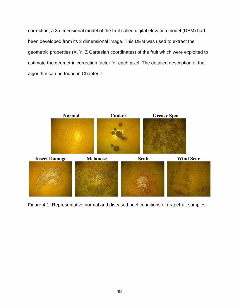
48
correction, a 3 dimensional model of the fruit called digital elevation model (DEM) had
been developed from its 2 dimensional image. This DEM was used to extract the
geometric properties (X, Y, Z Cartesian coordinates) of the fruit which were exploited to
estimate the geometric correction factor for each pixel. The detailed description of the
algorithm can be found in Chapter 7.
Figure 4-1: Representative normal and diseased peel conditions of grapefruit samples

49
Figure 4-2: Hyperspectral imaging system for reflectance image acquisition from grapefruits

50
Figure 4-3: Image classification procedure
Table 4-1: Numbers of fruit samples for each peel condition Peel
Condition Canker Normal Greasy Spot
Insect Damage Melanose Scab Wind
Scar Number 210 150 120 60 180 180 60

51
CHAPTER 5 ESTIMATION OF DETECTION LIMIT FOR SIZE OF CITRUS CANKER LESIONS
BASED ON HYPERSPECTRAL REFLECTANCE IMAGING
Introduction
Citrus canker is a serious disease that can infect most commercial citrus varieties.
Caused by bacterial pathogen Xanthomonas axonopodis, the disease is characterized
by conspicuous, erumpent lesions on leaves, stems, and fruit. Citrus canker originated
in Southeast Asia-India, and it has spread to Japan, South and Central Africa, the
Middle East, Australia, New Zealand, the Pacific Islands, South America, and Florida
(Schubert et al., 2001). Some areas of the world (e.g., South Africa, Australia, the Fiji
Islands, Mozambique, and New Zealand) have eradicated citrus canker. Eradication
programs have been implemented in infected areas such as Argentina, Uruguay, Brazil,
and Florida. Citrus canker could cause defoliation, blemished fruit, premature fruit drop,
twig dieback, and tree decline. Due to its fast spread, high damage potential, and
massive impact on export and domestic trade, canker is considered as one of the most
devastating diseases that threaten all citrus-growing areas.
Florida produces more than 70 percent of the citrus supply in the United States,
and it is the only growing region in the U.S. that is affected by canker. The Citrus
Canker Eradication Program (CCEP), initialized by the Florida Department of
Agriculture and Consumer Services - Division of Plant Industry (FDACS-DPI) and the
United States Department of Agriculture - Animal and Plant Health Inspection Service
(USDA-APHIS) in mid 1990’s, was an attempt to alleviate the consequences that canker
would have on the Florida citrus industry, as well as to keep other U.S. citrus-producing
areas (e.g., Texas and California) from being infected and harmed by this disease.
Because canker exhibits endemic features in most infected regions, there is no

52
universal treatment or prevention that could completely eradicate the disease in all the
infected areas. The current emphasis has been on minimizing the level of the disease
and preventing its further spread to the areas that are unaffected or were already
eradicated. Recently, the Florida eradication program has been terminated since citrus
canker is now considered endemic. In certain international canker-free markets, the
presence of cankerous fruit in a shipment could result in the whole shipment being
deemed unmarketable. It has been the common practice to detect citrus canker and
eliminate the infected fruit before they go to the market.
In recent years, Florida had been the only US state under quarantine for citrus
canker and therefore could not ship canker blemished fruit within the US or to other
countries those block shipment of canker infected fruit. In the fall of 2009, USDA APHIS
issued a new ruling based on research which demonstrated that canker cannot be
transmitted by infected fruit that had been treated with an appropriate disinfectant
(USDA APHIS, 2009). The ruling lifts the within US blockade and now allows free
shipment of disinfected fruit. However, there still remain several international markets
that have not lifted the ban on canker infected fruit to date.
Finding and removal of citrus fruit with canker is currently performed by human
inspectors in the packing house, which is labor-intensive and time-consuming.
Technologies that can efficiently identify citrus canker would assure fruit quality and
safety, which would enhance the competitiveness and profitability of the citrus industry.
Also sometimes the canker lesions are so small that they cannot be readily identified by
human eyes, and yet if such fruits are included in the shipment, they can cause the
entire shipment to be rejected at the port of entry into some markets. A number of

53
optical sensing techniques (e.g., machine vision and spectroscopy) have been
investigated to detect citrus-related diseases and defects, such as fruit blemish features
(Miller and Drouillard, 2001), leaf diseases (Pydipati et al., 2006), fruit surface defects
(Blasco et al., 2007), fruit rottenness (Gómez- Sanchis et al., 2008) and citrus canker
detection using limited number of hyperspectral wavelengths (Qin et al., 2009b).
However, only limited efforts have been made to detect the size of the smallest possible
canker affected lesion.
In the recent years, hyperspectral and multispectral imaging techniques have been
developed as useful tools for quality and safety evaluation of food and agricultural
products. The hyperspectral imaging technique acquires spatial information across a
sequence of individual band in a broad wavelength range, which generates a 3-D image
cube with a high spectral resolution. Although a large amount of spectral information is
useful for laboratory research, the hyperspectral cube contains redundant information
across tens or hundreds of bands. Consequently, real-time hyperspectral image
acquisition and processing is challenging due to the large amount of data.
Hyperspectral band selection, therefore, is usually performed to find a subset containing
few significant wavelengths (usually less than ten) with an aim of useful information
extraction and image dimensionality reduction.
Our recent studies (Qin et al., 2008, 2009a,b) have demonstrated that
hyperspectral imaging technique coupled with appropriate image processing and
classification methods [i.e., principal component analysis (PCA) and spectral
information divergence (SID), etc.] provides a useful means for detecting canker lesions
on citrus fruit. However, the full spectral information used by the PCA and SID

54
algorithms would limit their applications such as rapid on-line disease inspection due to
the large amount of 3-D hyperspectral data. Hence our team (Qin et al., 2009b) has built
a technique to select a set of hyperspectral bands for citrus canker detection using
multispectral algorithms in which the correlation analysis has been used to identify
important wavelengths for citrus canker detection based on hyperspectral reflectance
data. The objective of this particular research was to develop an algorithm to detect the
smallest possible canker affected lesion for real time online application, using the
previously urbanized multispectral algorithm.
Materials and Methods
Citrus Samples
Ruby Red grapefruits with normal surface, canker, and five common diseased peel
conditions (i.e., greasy spot, insect damage, melanose, scab, and wind scar) were
tested in this study. Color images for each typical peel condition are shown in Figure
5-1. The diseases on the fruit surface show different symptoms. Greasy spot, melanose,
and scab are all caused by fungi, which generate surface blemishes that are formed by
infection of immature fruit during the growing season. Greasy spot produces small
necrotic specks, and the affected areas are colored in brown to black and exhibit greasy
in appearance. Melanose is characterized by scattered raised pustules which are dark
brown to black in color. Scab appears as corky raised lesions usually with the color of
light brown. Different from the fungal diseases, citrus canker is caused by bacteria, and
it is featured with conspicuous dark lesions. Most circular in shape, canker lesions vary
in size and they are superficial (up to 1 mm deep) on the fruit peel (Timmer et al., 2000).
Diameter of the canker lesions tested in this study was approximately in the range of
1-9 mm. Insect damage is characterized by irregular grayish tracks on the fruit surface,

55
which are generated by larvae of leafminers that burrow under the epidermis of the fruit
rind. Wind scar, which is caused by leaves, twigs, or thorns rubbing against the fruit, is a
common physical injury on the fruit peel, and the scar tissue is generally gray.
Fruit samples were handpicked monthly from a grapefruit grove in Fort Pierce,
Florida during a seven-month harvest period from October 2007 to April 2008. Thirty
samples for each peel condition were collected for each month if the condition was
available. Cankerous samples were collected all seven months, and the samples with
other peel conditions were obtained every month according to their availabilities. The
grapefruit samples with different sizes of canker lesions were used to evaluate the size
detection limits for hyperspectral image processing and classification methods.
A total of 960 grapefruits were collected and tested in this study. Numbers of
samples for each peel condition are summarized in Table 5-1. All the grapefruits were
washed and treated with chlorine and sodium o-phenylphenate (SOPP) at the Indian
River Research and Education Center of University of Florida (UF) in Fort Pierce,
Florida. The samples were transported to UF campus in Gainesville, Florida, and stored
in an environmental control chamber maintained at 4 ºC. The samples were removed
from cold storage about 2 hours before imaging to allow them to reach room
temperature. During image acquisition, the fruit samples were placed in rubber cups
attached to the linear positioning table, with lesions facing upward, to insure that the
diseased areas were in the imaging systems field of view.
Hyperspectral Imaging System
A hyperspectral imaging system was used to acquire reflectance images from
citrus samples. A schematic diagram of the system is illustrated in Figure 5-2. This
hyperspectral imaging system was developed in cooperation with the USDA

56
Environmental Microbial and Food Safety Laboratory in Beltsville, MD, and is
conceptually similar to the system reported in Qin et al. (2008). It is a push broom, line-
scan based imaging system that utilizes an electron-multiplying charge-coupled-device
(EMCCD) camera (iXon, Andor Technology Inc., South Windsor, CT, USA). The
EMCCD has 1004×1002 pixels and is thermoelectrically cooled to -80°C through a
double-stage Peltier device. An imaging spectrograph (ImSpector V10E, Spectral
Imaging Ltd., Oulu, Finland) and a C-mount zoom lens (Rainbow CCTV H6X8,
International Space Optics, S.A., Irvine, CA, USA) are mounted to the camera. The
instantaneous field of view (IFOV) is limited to a thin line by the spectrograph aperture
slit (30 μm), and the spectral resolution of the imaging spectrograph is 2.8 nm. Through
the slit, light from the scanned IFOV line is dispersed by a prism-grating-prism device
and projected onto the EMCCD. Therefore, for each line-scan, a two-dimensional
(spatial and spectral) image is created with the spatial dimension along the horizontal
axis and the spectral dimension along the vertical axis of the EMCCD. The lighting unit
consists of two 21 V, 150 W halogen lamps powered with a DC voltage regulated power
supply (TechniQuip, Danville, CA, USA). The light is transmitted through optical fiber
bundles toward line light distributors. Two line lights are arranged to illuminate the IFOV.
A programmable, motorized positioning table (BiSlide-MN10, Velmex Inc., Bloomfield,
NY, USA) moves citrus samples (five for each run) transversely through the line of the
IFOV. One thousand seven hundred and forty line scans were performed for five fruit
samples, and 400 pixels covering the scene of the fruit at each scan were saved,
generating a 3-D hyperspectral image cube with the spatial dimension of 1740×400 for
each band. Spectral calibration of the system was performed using an Hg-Ne spectral

57
calibration lamp (Oriel Instruments, Stratford, CT, USA). Because of inefficiencies of the
system at certain wavelength regions (e.g., low light output in the visible region less
than 450 nm, and low quantum efficiency of the EMCCD in the NIR region beyond 930
nm), only the wavelength range between 450 and 930 nm (totaling 92 bands with a
spectral resolution of 5.2 nm) was used in this investigation. The parameterization and
data-transfer interface software for the hyperspectral imaging system were developed
using a SDK (Software Development Kit) provided by the camera manufacturer on a
Microsoft Visual Basic (Version 6.0) platform in the Windows operating system.
Image Pre-Processing
As mentioned in the earlier section (Hyperspectral Imaging System), each
hyperspectral image taken with our system consists of 3-D hyperspectral image cube
with spatial dimension of 1740×400 and spectral dimension of 92 (92 wavelengths). To
reduce the amount of data for computation, spatial binning technique was used in which
the hyperspectral image data was averaged by two neighboring pixels in both vertical
and horizontal spatial dimensions at each wavelength. This reduced the size of the
original 3-D image data from 1740×400×92 (92 bands) to 870×200×92, and resulted in
a spatial resolution of 0.6 mm/pixel for both vertical and horizontal dimensions. The
image preprocessing procedures described above were executed using programs
developed in MATLAB R2007a (Math Works, Natick, MA, USA). Along with this the
image preprocessing was performed for the original hyperspectral reflectance images to
fulfill flat-field correction and image masking which resulted in normalized and masked
hyperspectral cubes with a dimension of 870×200×92 (92 bands). Detailed procedures
for hyperspectral image preprocessing can be found in Qin et al. (2008).

58
Hyperspectral Band Selection
The goal of this research was to determine the minimum size limit at which citrus
canker lesions can be reliably detected for real time packing line applications. However,
we must first have an effective approach to segregate cankerous citrus fruits from
normal peel or other surface defects. The disease defect classification approach
implemented in this study used a real-time multispectral algorithm based on correlation
analysis for band selection (Qin et al., 2009b).
Even after preprocessing the image data, the 3-D hyperspectral data
(870×200×92) is still too large for rapid real time applications and hence a multispectral
algorithm is needed that uses a subset of the hyperspectral data to reduce the
computation time thus making it more suitable for online applications. The multispectral
algorithm exploits correlation analysis (CA) to select the optimal pair of wavelengths that
can be used to distinguish between cankered, normal, and other diseased peel
conditions. In this method, the selected optimal pair of wavelengths is used to create the
two band ratio image (i.e., Rλ1/Rλ2, where Rλn denotes single band reflectance image at
the wavelength λn) which helps us to make the distinction. Ratio method was chosen
because the ratio images are invariant to illumination scaling, which is a significant
advantage for real-time applications. All 960 fruit samples were divided into two classes:
‘Canker’ class including 210 samples with canker lesions, and ‘No Canker’ class
including 150 normal samples and 600 samples with other five peel diseases (see Table
5-1). To facilitate correlation analysis, samples in the ‘Canker’ class were labeled with
‘1’, and ‘No Canker’ class with ‘0’. Correlation coefficients were calculated between two
band ratios of the ROI spectra and the fruit label values (i.e., 1 and 0) in an exhaustive
way (i.e., evaluating all possible two band combinations from 92 wavelengths). The pair

59
of wavelengths which gave the maximum value for the correlation coefficient (the
optimum pair previously mentioned) was selected for further classification and lesion
size estimation.
Keeping in mind that selecting more additional wavelengths may (or may not)
improve classification accuracies, the third and forth bands were identified by
performing the correlation analysis in a sequential forward way. The third band (i.e., Rλ3)
was determined by the highest correlation between the fruit label values and ratio
values calculated in a form of (Rλ1 - Rλ3)/(Rλ2 - Rλ3), where Rλ1 and Rλ2 were two best
bands selected from the previous correlation analysis. After the third band was
determined, the fourth band was identified using the similar method on two forms of
ratio calculations: (Rλ1 - Rλ3)/(Rλ2 - Rλ4a) and (Rλ1 - Rλ4b)/(Rλ2 - Rλ3), where Rλ1, Rλ2, and
Rλ3 were determined from the previous procedures, and Rλ4a and Rλ4b were newly
selected bands from the highest correlations. However, as demonstrated in previous
studies (Qin et al., 2009b), the two band ratio method gives the best overall
classification results and hence this study is an extension of the earlier two band ratio
approach. The two bands ratio of 834 nm and 729 nm (R834/R729) was found to give the
maximum absolute value for the correlation coefficient of 0.811 and hence was chosen
to be the optimal pair of wavelengths to discriminate between fruit exhibiting cankerous
and other peel conditions. The detailed procedure for selecting the optimal pair of
wavelengths can be found in Qin et al. (2009b).
Image Classification
After identifying important wavelengths using CA, band ratio images were
generated using ENVI 4.3 software (ITT Visual Information Solutions, Boulder, CO,
USA) and the selected wavelength’s single band images. The equation Rλ1/Rλ2 (i.e.,

60
R834/R729) was used to create these new ratio images. A simple thresholding approach,
which has been used to differentiate cancerous fruits from six other peel conditions
(normal peel and other citrus diseases), was applied to the ratio images calculated
using the above equations. Different threshold values were used to evaluate
classification accuracies for canker identification. A Morphological filtering operation
followed thresholding, in order to remove undesirable noise (small pixel regions
attributed to edge affects and other peel conditions) from the image as these small pixel
regions can result in an increase in false positives. It is recognized that this filtering
operation can inhibit detection of very small canker lesions, and thus creates a tradeoff
between the number of false positives, and false negatives. The morphological
“opening” operation was applied to the thresholded image, which by definition means
erosion of the image followed by subsequent dilation. The opening filter from the ENVI
morphological filter tools with a kernel size of 3×3 was selected. The purpose of erosion
is to remove the undesired small size pixels, with dilation smoothening out the contours
of the remaining pixel areas to help restore the round feature of the canker lesions in
the final binary images.
Binary Lesion Size Detection Algorithm
To determine the smallest canker lesion detected by the above mentioned image
classification algorithm, the classified images (Final Binary Images) of the samples were
examined. For this task also morphological opening operation was used. The function
‘bwareaopen’ in MATLAB R2007a (Math Works, Natick, MA, USA) was used to
determine the number of pixels in the smallest canker lesion detected during the
classification process. The function ‘bwareaopen’ removes all connected components
(objects) from a binary image that have fewer than certain number of pixels defined in

61
the syntax, producing another binary image. The number of pixels defined in the syntax
was incremented by one at a time and the image before and after applying
‘bwareaopen’ function were compared for consistency. Whenever some difference was
observed between the two images, the number of pixels (defined in syntax of
‘bwareaopen’) was noted. This pixel count minus one represented the number of pixels
(N’) in the smallest canker lesion detected in the binary image by the lesion size
estimation algorithm.
Mapping Binary Lesion Size to Original Hyperspectral Image
The smallest size lesions obtained by following the above procedure were found in
the binary image. Consequently, to obtain an accurate size estimate for the smallest
lesion, it was necessary to map the lesion found in the binary image back to the
un-eroded lesion in the original hyperspectral image. This was done using ENVI. The X
and Y coordinates of the centriod of binary canker lesion (which was detected to be the
smallest) were estimated using MATLAB and corresponding lesion in the original
hyperspectral image was located. The number of pixels (N) in the original hyperspectral
image lesion was counted using the region of interest (ROI) tool in Basic Tools of ENVI.
The spatial resolution of the images was 0.6 mm/pixel in horizontal direction and
0.6 mm/pixel in vertical direction. Hence the surface area of one pixel is 0.6×0.6 sq.
mm. Accordingly the surface area of the smallest canker lesion (A) was computed from
the number of pixels in the lesion and area per pixel. Then assuming that most canker
lesions are approximately circular in shape, the equivalent diameter (d) of the lesion
was computed from the following formula:
A = πd2/4 (5-1)

62
Results, Observations and Discussion
Image Classification Results
As demonstrated in a previous study (Qin et al., 2009b) it is not possible to detect
the citrus canker using a single wavelength, and hence a multispectral imaging solution
utilizing information acquired from the hyperspectral bands was developed. The
multispectral algorithm explained in previous sections is illustrated in Figure 5-3, where
the various image processing steps necessary to generate the final thresholded binary
image of a canker infected fruit is shown. In this approach, the two band ratio method
(R834/R729) has been applied. As mentioned previously, an important fact that should be
remembered is that small cankerous lesions (very few pixels) may be removed along
with the undesired pixel noise during the erosion operation. This can be observed in
Figure 5-3, where two very small lesions in the ‘Binary image’ (image after thresholding)
disappeared after the morphological opening operation in the ‘Final Binary image’.
Hence there is risk of removing small canker lesions when filtering resulting in an
increase in false negatives. In Figure 5-4, the algorithm’s ability to discriminate between
canker and other peel conditions is shown. One should note that the images of
individual grapefruits in Figure 5-4 were acquired separately and a mosaic containing
seven samples was generated to reveal capability of canker detection. As can be seen
in Figure 5-4, the ‘Final Binary Image’ (after morphological opening) contains white
pixels at canker lesions locations, while all other pixels were thresholded to black.
The effect of varying threshold values on classification accuracy was analyzed for
threshold values ranging from 1.20 to 1.35 for all two band ratio images. It was
observed that the threshold value of 1.20 gave the best canker detection accuracy of
99.05% with the overall accuracy of 89.17%. On the other hand a higher threshold value

63
of 1.35 did a better job in terms of overall accuracy (93.13%) (but not the best overall
accuracy), meanwhile the canker detection accuracy was reduced to 77.62%. The
reason behind this was, as we increased the threshold value the smaller canker lesions
were eliminated thus increasing the false negative errors. The result of variation of
threshold value on classification can be easily observed from the graph in Figure 5-5.
We can conclude from graph that, canker classification accuracy diminishes with
increasing threshold value (due to filtering out smallest canker lesions); on the other
hand the overall accuracy shows opposite trend, increasing with threshold value.
However, after a certain threshold value, the overall accuracy also starts dropping as
canker misclassification increases at higher threshold values. The threshold value of
1.275 appears to give best tradeoff between canker classification accuracy (94.3%) and
overall classification (95.7%). Table 5-2 summarizes these classification results for the
two band ratio method. So, when evaluating lesion detection size limits, one should
keep in mind that along with the number of erosion cycles, excessively high values of
threshold can also result in increased misclassification and thus poor estimation of the
size of the smallest detectable canker lesion.
Binary Lesion Size Estimation Results
After classifying all citrus fruits as either “canker” or “no Canker”, the MATLAB
algorithm (using ‘bwareaopen’) was applied to detect the smallest cankerous lesion.
Figure 5-6 shows the zoomed images of the same sample as in Figure 5-3, before and
after applying the ‘bwareaopen’ function. As can be seen from Figure 5-6, two lesions in
the left image have disappeared in the right image due to application of the function
‘bwareaopen’. These two lesions were the smallest lesions detected by our algorithm.
One should not get confused between the application of erosion in the opening filter and

64
the use of MATLAB function ‘bwareaopen’. We made use of the morphological opening
filter to get rid of unwanted pixels like edges and other minor peel disease conditions,
which is a normal filtering approach that would be implemented in the online detection
system. On the other hand, the function ‘bwareaopen’ was simply used as an analysis
tool to assist in detecting the smallest cankerous lesion present in the binary image.
Two most important factors which influence the estimation of the smallest canker
lesion present are, 1} the number of erosion cycles used in the morphological opening
operation and 2} the threshold value used in image classification. The effect of variation
of threshold values on the lesion size study is already evident from the classification
results (refer Figure 5-5). As we increase the threshold value, small sized and lighter
canker lesions were removed from the final binary image resulting in reduced
classification accuracy because of increased false negative errors.
The effect of the number of erosion cycles is explained in Table 5-3, which shows
a classification summary for 210 cankerous grapefruit samples with a threshold of 1.275
and different number of erosion cycles. As the number of erosion cycles is increased
from 1 to 5, our classification results vary from 94.29% to 11.90%, respectively. Also if
we look at the size of smallest lesion detected in terms of number of pixels, the size can
be seen increasing with the number of erosion cycles. The reason behind this was the
small sized and lighter lesions were removed by the increased number of erosion
cycles. In this study, a single erosion cycle and a classification threshold of 1.275 has
been used to avoid increasing false negative errors of classification.
Results of Mapping Binary Lesion Size to Original Hyperspectral Image
Figure 5-7 portrays the process of mapping the binary canker lesion to the original
hyperspectral image. As can be seen, the image at center shows the detected lesion in

65
binary image. The corresponding original lesion is encircled in the left image. The right
most image shows the same lesion being located in the original hyperspectral image
and region of interest (ROI) being grown (red in color) using ENVI’s ROI tool to
calculate the number of pixels in the actual canker lesion in the original hyperspectral
image. Each one of the 210 cankerous grapefruit samples was examined and the
smallest canker lesion was detected in the corresponding binary images and then
mapped back to the original hyperspectral image. The plot in Figure 5-8 shows
probability distribution of the actual canker lesion size in pixels.
As can be seen from Figure 5-8, most of the data is concentrated in the lesion size
range of 6 to 35 pixels and the plot could be approximated by a ‘Log-Normal’
distribution. Contrary to the characteristics of a Normal or Gaussian distribution this data
set does not exhibit a central tendency and thus has some other probability distribution.
However, we can observe that the mode of the dataset corresponds to the lesion size
range of 8 to 14 pixels with a frequency of occurrence of 37 out of 210, while 73 out of
210 would fall in the range of 8 to 21. This suggests that when using the optimal number
of erosions and threshold, the two-band classification approach is consistently
classifying lesions in this size range at above 94% accuracy. Figure 5-9 shows more
details of the encircled part of the plot in Figure 5-8.
The size of the smallest canker lesion, in terms of surface area (sq. mm.) was
determined utilizing the spatial resolution of each pixel (0.6 mm in both horizontal and
vertical directions) as,
A = Number of pixels in smallest lesion × 0.6 mm × 0.6 mm (5-2)
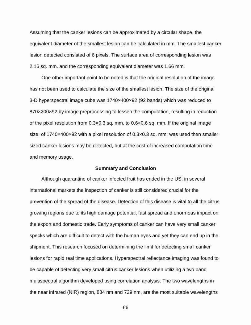
66
Assuming that the canker lesions can be approximated by a circular shape, the
equivalent diameter of the smallest lesion can be calculated in mm. The smallest canker
lesion detected consisted of 6 pixels. The surface area of corresponding lesion was
2.16 sq. mm. and the corresponding equivalent diameter was 1.66 mm.
One other important point to be noted is that the original resolution of the image
has not been used to calculate the size of the smallest lesion. The size of the original
3-D hyperspectral image cube was 1740×400×92 (92 bands) which was reduced to
870×200×92 by image preprocessing to lessen the computation, resulting in reduction
of the pixel resolution from 0.3×0.3 sq. mm. to 0.6×0.6 sq. mm. If the original image
size, of 1740×400×92 with a pixel resolution of 0.3×0.3 sq. mm, was used then smaller
sized canker lesions may be detected, but at the cost of increased computation time
and memory usage.
Summary and Conclusion
Although quarantine of canker infected fruit has ended in the US, in several
international markets the inspection of canker is still considered crucial for the
prevention of the spread of the disease. Detection of this disease is vital to all the citrus
growing regions due to its high damage potential, fast spread and enormous impact on
the export and domestic trade. Early symptoms of canker can have very small canker
specks which are difficult to detect with the human eyes and yet they can end up in the
shipment. This research focused on determining the limit for detecting small canker
lesions for rapid real time applications. Hyperspectral reflectance imaging was found to
be capable of detecting very small citrus canker lesions when utilizing a two band
multispectral algorithm developed using correlation analysis. The two wavelengths in
the near infrared (NIR) region, 834 nm and 729 nm, are the most suitable wavelengths

67
to detect cankerous lesions. The ratio of reflectance for these two wavelengths along
with a simple thresholding and morphological opening approach forms the basis for
canker detection. It was observed that smaller values of thresholds gave better canker
classification accuracy (up to 99%), while giving a lower overall accuracy (89%). On the
other hand, the trend was opposite for higher threshold values. Also as the numbers of
erosion cycles were increased, the classification accuracy dropped drastically, as the
small canker lesions were removed by the erosion operation. Therefore, the minimum
canker lesion sizes detected at a higher number of erosion cycles were significantly
larger than those detected at a fewer number of erosion cycles. The threshold value of
1.275 and a single erosion cycle in the opening filter gave the optimum classification
accuracy. The best overall classification accuracy was found to be 95.7%. The statistics
of the lesion size showed that the probability distribution is approximately log-normal
and hence we cannot use central tendency as a representative of the data. Most
minimum lesion size data accumulated in the low pixel range (6-35 pixels in number).
The grape fruit samples with canker lesions as small as 6 pixels in size were classified
accurately. The corresponding size of the smallest cankerous lesion in terms of surface
area was 2.16 sq. mm. and in terms of equivalent diameter was 1.66 mm. The
resolution of a pixel used in this study was 0.6×0.6 sq. mm. If we use higher resolution
images, we should able to detect even smaller canker lesions than that detected during
this study.

68
Figure 5-1: Representative normal and diseased peel conditions of grapefruit samples

69
Figure 5-2: Hyperspectral imaging system for reflectance image acquisition from grapefruits

70
Figure 5-3: Image Classification Procedure
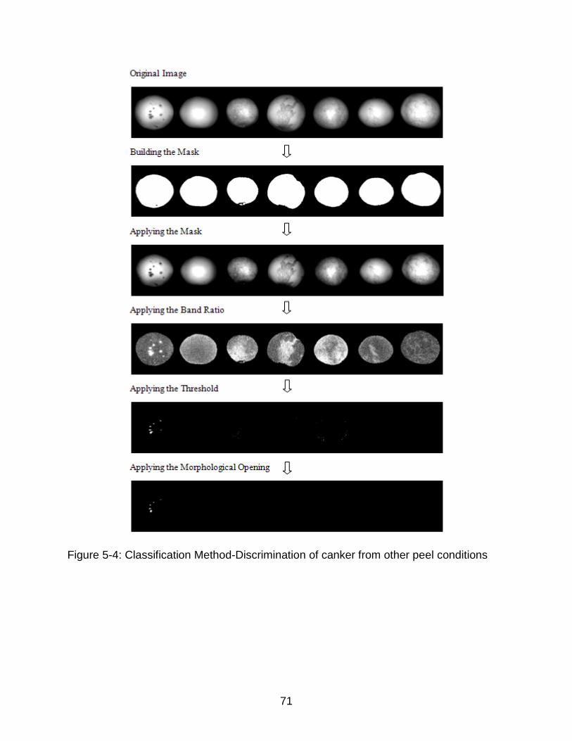
71
Figure 5-4: Classification Method-Discrimination of canker from other peel conditions

72
Figure 5-5: Effect of variation of threshold values on classification accuracies
Figure 5-6: Final Binary Image of a sample before and after applying the ‘bwareaopen’ function
75
80
85
90
95
100
1.200 1.250 1.275 1.280 1.300 1.350
Cla
ssifi
catio
n A
ccur
acy
(%)
Threshold
Canker
Overall

73
Original Image Final Binary Image Mapped Lesion
Figure 5-7: Mapping binary lesion size to original hyperspectral image
Figure 5-8: Probability distribution of lesion size of all samples
0
5
10
15
20
25
30
35
40
0-7
15-2
1
29-3
5
43-4
9
57-6
3
71-7
7
85-9
1
99-1
05
113-
119
127-
133
141-
147
155-
161
169-
175
183-
189
197-
203
210-
abov
e
Freq
uenc
y
Original Lesion Size (Pixels)

74
Figure 5-9: Probability distribution of lesion size of subset of all samples
Table 5-1: Numbers of fruit samples for each peel condition
Peel Condition Canker Normal Greasy
Spot Insect
Damage Melanose Scab Wind Scar
Number 210 150 120 60 180 180 60
Table 5-2: Summary of classification results
Disease Number of Samples
Rule Classifier Threshold
Number of Misclassified
Classification accuracy (%)
Canker 210 1.275 12* 94.29 Greasy spot 120 1.275 12 90.00
Insect damage 60 1.275 1 98.33 Melanose 180 1.275 10 94.44
Scab 180 1.275 5 97.22 Wind scar 60 1.275 0 100.00
Market 150 1.275 1 99.33 Overall 960 41 95.73
* Represents the number of misclassified canker samples out of the total of 210 canker infected samples.
0
5
10
15
20
25
30
35
40
0-7
8-14
15-2
1
22-2
8
29-3
5
36-4
2
43-4
9
50-5
6
57-6
3
64-7
0
71-7
7
78-8
4
85-9
1
92-9
8
Freq
uenc
y
Original Lesion Size (Pixels)

75
Table 5-3: Effect of number of erosion cycles on canker lesion size estimation Number of Erosion
Cycles Number of
Misclassified Samples1 Canker Classification
Accuracy (%) No. of Pixels in Smallest Lesion
1 12 94.29 5 2 60 71.43 13 3 109 48.10 25 4 162 22.86 41 5 185 11.90 61
1 Represents the number of misclassified canker samples out of the total of 210 canker infected samples.

76
CHAPTER 6 DETECTION OF CITRUS CANKER USING RGB COLOR IMAGE ALONG WITH
NEAR-INFRARED MONOCHROME IMAGES
Introduction
Citrus canker is one of the most devastating diseases that the citrus industry is
presently fighting with. Citrus canker which is caused by bacterial pathogen
Xanthomonas axonopodis, is spread almost all over the world. However few areas like
South Africa, Australia, the Fiji Islands, Mozambique, and New Zealand have been
proven successful for eradicating canker completely. Active ongoing eradication
programs still continue in other infected areas such as Argentina, Uruguay, Brazil, and
Florida. Due to its fast spread, high damage potential, and massive impact on export
and domestic trade, canker is considered as one of the most disturbing diseases that
threaten all citrus-growing areas.
Florida which produces more than 70% of citrus supply is the only region in United
States which is under the influence of this disease. It is really difficult to eradicate
canker completely from all the infected regions and hence the present objective of
Citrus Canker Eradication Program (CCEP) is to minimize the level of disease and to
prevent the spread of the disease to the unaffected or already eradicated area. The
presence of cankerous fruit in a shipment could result in the whole shipment being
deemed unmarketable to some ‘canker-free’ areas, such as the European countries. It
is therefore crucial to detect citrus canker and eliminate the infected fruit before they go
to the market.
Present human inspection is labor intensive and time consuming. Also it is
subjected to the skill level of the labor. So the need of an automated disease detection
system gets highlighted. Some machine vision and image processing related

77
approaches have been used by different researchers to detect defects on the biological
items like fruits and leaves which include citrus disease detection using color texture
features and discriminant analysis (Pydipati et al., 2006), poultry carcasses defect
detection using co-occurrence texture features (Park and Chen, 2000), statistical and
neural network classifier for citrus disease detection (Pydipati et al., 2005), classification
of different weed species using color co-occurrence method and neural network
classifier (Burks et al., 2000), and many more.
In the recent years, hyperspectral and multispectral imaging techniques have been
developed as useful tools for quality and safety evaluation of food and agricultural
products. The hyperspectral imaging technique acquires spatial information across a
sequence of individual band in a broad wavelength range, which generates a 3-D image
cube with a high spectral resolution. Although plenty spectral information is fairly useful
for laboratory research, the hyperspectral cube contains redundant information across
tens or hundreds of bands. Consequently, real-time hyperspectral image acquisition and
processing is challenging due to the large amount of data. Hyperspectral band
selection, therefore, is usually performed to find a subset containing few significant
wavelengths (usually less than ten) with an aim of useful information extraction and
image dimensionality reduction. Such attempts using hyperspectral and multispectral
imaging include bruises detection on apples using NIR hyperspectral imaging (Lu,
2002), online defect and fecal contamination detection on apples (Kim et al., 2007),
multispectral wavelength selection using correlation analysis for detection of defects on
apples (Lee et al., 2008), wavelength selection for discriminating weeds from crop
(Piron et al., 2007), PCA based image classification for citrus canker detection (Qin et

78
al., 2008), multispectral wavelength selection for citrus canker detection using
correlation analysis (Qin et al., 2009) etc.
The literature also reveals that RGB color images, with or without hyperspectral /
multispectral imaging, have been successfully used to detect defects, physical damages
and diseases on the biological produce. Stem ends and sooty mold conditions can also
be separated from diseases condition using RGB color imaging. Noordam et al. (2005)
made use of RGB color images along with multispectral images to detect the latent
defects and diseases on raw French fries. Kim et al. (2009) also used high resolution
RGB images of citrus fruits and leaves to detect the presence of canker and greening
diseases.
Our research team (Qin et al., 2009) has recently developed an algorithm for real
time online detection of the cankerous fruits using two monochrome camera
assemblies. The two wavelengths of the cameras were selected by applying the
correlation analysis to the 3-D hyperspectral image cube. However, it is needless to
mention that a single 3-CCD camera is definitely cheaper than multiple monochrome
cameras required for capturing the independent single band multispectral images or
electron multiplying charge-coupled-device (EMCCD) camera assemblies required for
acquiring hyperspectral images. So this particular exploration was aimed at
investigating if one of the monochrome cameras can be replaced by a CCD camera so
that RGB color image can be used in conjunction with a monochrome image to detect
cankerous citrus fruit. This novel two camera system (with one CCD color camera and
other monochrome camera) then would allow us to exploit the RGB color image for
other detection tasks like sooty mold detection, physical damage detection etc. as well.
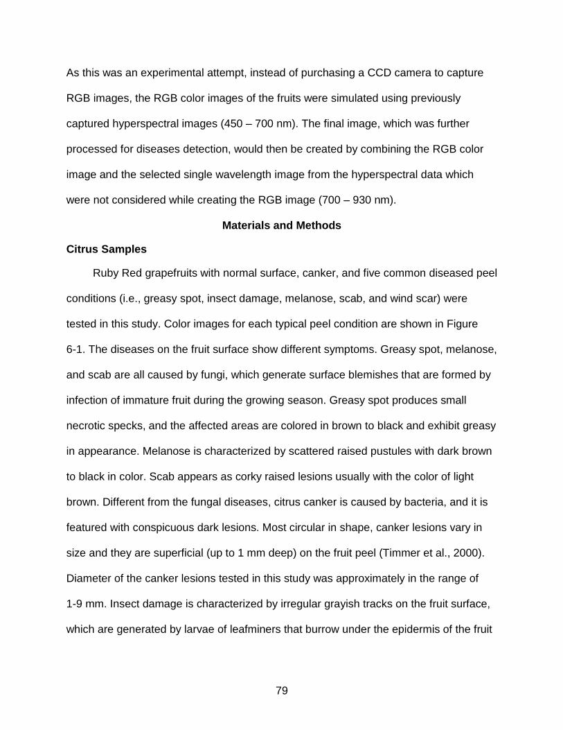
79
As this was an experimental attempt, instead of purchasing a CCD camera to capture
RGB images, the RGB color images of the fruits were simulated using previously
captured hyperspectral images (450 – 700 nm). The final image, which was further
processed for diseases detection, would then be created by combining the RGB color
image and the selected single wavelength image from the hyperspectral data which
were not considered while creating the RGB image (700 – 930 nm).
Materials and Methods
Citrus Samples
Ruby Red grapefruits with normal surface, canker, and five common diseased peel
conditions (i.e., greasy spot, insect damage, melanose, scab, and wind scar) were
tested in this study. Color images for each typical peel condition are shown in Figure
6-1. The diseases on the fruit surface show different symptoms. Greasy spot, melanose,
and scab are all caused by fungi, which generate surface blemishes that are formed by
infection of immature fruit during the growing season. Greasy spot produces small
necrotic specks, and the affected areas are colored in brown to black and exhibit greasy
in appearance. Melanose is characterized by scattered raised pustules with dark brown
to black in color. Scab appears as corky raised lesions usually with the color of light
brown. Different from the fungal diseases, citrus canker is caused by bacteria, and it is
featured with conspicuous dark lesions. Most circular in shape, canker lesions vary in
size and they are superficial (up to 1 mm deep) on the fruit peel (Timmer et al., 2000).
Diameter of the canker lesions tested in this study was approximately in the range of
1-9 mm. Insect damage is characterized by irregular grayish tracks on the fruit surface,
which are generated by larvae of leafminers that burrow under the epidermis of the fruit

80
rind. Wind scar, which is caused by leaves, twigs, or thorns rubbing against the fruit, is a
common physical injury on the fruit peel, and the scar tissue is generally gray.
Fruit samples were handpicked monthly from a grapefruit grove in Fort Pierce,
Florida during a seven-month harvest period from October 2007 to April 2008. Thirty
samples for each peel condition were collected for each month if the condition was
available. Cankerous samples were collected all seven months, and the samples with
other peel conditions were not obtained every month due to their availabilities. The
grapefruit samples with different sizes of canker lesions were used to evaluate the size
detection limits for hyperspectral image processing and classification methods.
A total of 960 grapefruits were collected and tested in this study. Numbers of
samples for each peel condition are summarized in Table 6-1. All the grapefruits were
washed and treated with chlorine and sodium o-phenylphenate (SOPP) at the Indian
River Research and Education Center of University of Florida (UF) in Fort Pierce,
Florida. The samples were transported to UF campus in Gainesville, Florida, and stored
in an environmental control chamber maintained at 4 ºC. The samples were removed
from cold storage about 2 hours before imaging to allow them to reach room
temperature. During image acquisition, the fruit samples were placed on the rubber
cups, which were fixed on the positioning table of the imaging system, to make sure the
diseased areas were on the top of each fruit.
Hyperspectral Imaging System
A hyperspectral imaging system was used to acquire reflectance images from
citrus samples. Schematic diagram of the system is illustrated in Figure 6-2. It is a push
broom, line-scan based imaging system that utilizes an electron multiplying charge-
coupled-device (EMCCD) camera (iXon, Andor Technology Inc., South Windsor, CT,

81
USA). The EMCCD has 1004×1002 pixels and is thermoelectrically cooled to -80°C
through a double-stage Peltier device. An imaging spectrograph (ImSpector V10E,
Spectral Imaging Ltd., Oulu, Finland) and a C-mount zoom lens (Rainbow CCTV H6X8,
International Space Optics, S.A., Irvine, CA, USA) are mounted to the camera. The
instantaneous field of view (IFOV) is limited to a thin line by the spectrograph aperture
slit (30 μm), and the spectral resolution of the imaging spectrograph is 2.8 nm. Through
the slit, light from the scanned IFOV line is dispersed by a prism-grating-prism device
and projected onto the EMCCD. Therefore, for each line-scan, a two-dimensional
(spatial and spectral) image is created with the spatial dimension along the horizontal
axis and the spectral dimension along the vertical axis of the EMCCD. The lighting unit
consists of two 21 V, 150 W halogen lamps powered with a DC voltage regulated power
supply (TechniQuip, Danville, CA, USA). The light is transmitted through optical fiber
bundles toward line light distributors. Two line lights are arranged to illuminate the IFOV.
A programmable, motorized positioning table (BiSlide-MN10, Velmex Inc., Bloomfield,
NY, USA) moves citrus samples (five for each run) transversely through the line of the
IFOV. One thousand seven hundred and forty line scans were performed for five fruit
samples, and 400 pixels covering the scene of the fruit at each scan were saved,
generating a 3-D hyperspectral image cube with the spatial dimension of 1740×400 for
each band. Spectral calibration of the system was performed using an Hg-Ne spectral
calibration lamp (Oriel Instruments, Stratford, CT, USA). Because of inefficiencies of the
system at certain wavelength regions (e.g., low light output in the visible region less
than 450 nm, and low quantum efficiency of the EMCCD in the NIR region beyond 930
nm), only the wavelength range between 450 and 930 nm (totaling 92 bands with a

82
spectral resolution of 5.2 nm) was used in this investigation. The parameterization and
data-transfer interface software for the hyperspectral imaging system were developed
using a SDK (Software Development Kit) provided by the camera manufacturer on a
Microsoft Visual Basic (Version 6.0) platform in the Windows operating system.
Image Pre-Processing
As mentioned in the earlier section (Hyperspectral Imaging System), each
hyperspectral image taken with our system consists of 3-D hyperspectral image cube
with spatial dimension of 1740×400 and spectral dimension of 92 (92 wavelengths). To
reduce the amount of data for computation, the binning technique was used in which the
hyperspectral image data was averaged by two neighboring pixels in both vertical and
horizontal spatial dimensions at each wavelength. This reduced the size of the original
3-D image data from 1740×400×92 (92 bands) to 870×200×92, and resulted in a spatial
resolution of 0.6 mm/pixel for both vertical and horizontal dimensions. The image
preprocessing procedures described above were executed using programs developed
in MATLAB R2007a (Math Works, Natick, MA, USA). Along with this the image
preprocessing was performed for the original hyperspectral reflectance images to fulfill
flat- field correction and image masking which resulted in normalized and masked
hyperspectral cubes with a dimension of 870×200×92 (92 bands). Detailed procedures
for hyperspectral image preprocessing can be found in Qin et al. (2008).
Simulation of RGB Color Image
When white light falls on the 3-CCD camera lens, the lens amplifies the incoming
signal (light) and this signal is filtered through the Red, Green and Blue filters’ assembly
so that only red / green / blue light is directed to the respective CCD chips. The CCD
chips generate the signals proportional to the light falling on them which when

83
processed by camera electronics, the red, green and blue channels of the digital image
are created (The Imaging source, 2005). The similar principle was employed while
simulating the red, green and blue channels for this study. The filter characteristics were
simulated and the resulting filter was applied to previously captured hyperspectral
images to generate the red, green and blue response of the image.
First of all, the transmission characteristics of the red, green and blue filters were
assumed to have a Gaussian bell shape in the wavelength range of 600-700 nm,
500-600 nm and 400-500 nm, respectively with corresponding means at 650, 550 and
450 nm (Kondo and Ting, 1998). These filter characteristics were then simulated using
MATLAB R2009a and are presented in Figure 6-3. These filters were then applied to
the monochrome images of respective wavelength ranges from the 3-D hyperspectral
image cube. The filter characteristics gave a particular value of transmittance for every
wavelength in the respective red, green and blue range. The monochrome image of a
particular wavelength was then multiplied by the corresponding transmittance value.
The monochrome images in the range 600-700 nm, 500-600 nm and 400-500 nm
processed in this way were combined together (taking average of all the monochrome
images in a particular channel) to generate the red, green and blue channels of the
RGB image.
Combining RGB Color Image and Remaining Monochrome Images
As mentioned earlier the hyperspectral images were captured in the range of 450
to 930 nm. The simulated RGB image had considered the wavelengths in the range of
450 to 700 nm. So the remaining wavelengths (700-930 nm) were combined with the
simulated red, green and blue channels so as to create a new hyperspectral image.
This new hyperspectral RGB + NIR simulated image had 46 bands or channels, the first
84
three of them were red, green and blue while the remaining 43 were the single band
images at respective wavelengths in the range 700 to 930 nm. So this hyperspectral
image of size 870×200×46 (46 bands) was used for further analysis.
Hyperspectral Band Selection
After simulating the RGB color image and combining it with the single band
images as explained in previous section, the resulting hyperspectral image was of size
870×200×46 (46 bands). Even if this image was of size smaller than the previous one
(870×200×92), this size was still too large from computation point of view. Hence to
obtain computationally viable approach, previously developed multispectral algorithm
(Qin et al., 2009) was used to select optimal wavelengths by applying correlation
analysis to hyperspectral image cube of size 870×200×46. The main objective was to
observe if the correlation analysis picks any of the red, green or blue channels along
with some NIR wavelength for identifying canker.
The correlation analysis (CA) helps to select an optimal pair of wavelengths which
can be used to segregate the cankered citrus fruits from normal or other peel
conditions. First of all the reflectance spectra of canker, normal and five other disease
conditions (greasy spot, insect damage, melanose, scab and wind scar) were extracted
using ENVI 4.3 software (ITT Visual Information Solutions, Boulder, CO, USA). Instead
of extracting the reflectance spectra from a single pixel of respective peel condition, it
was acquired by averaging over number of pixels by using the region of interest (ROI)
tool in ENVI. The ROI was manually selected in the zoom window that contains typical
diseased or normal peel areas using various drawing methods (e.g., polygon, rectangle,
ellipse, point, grow, and merge) offered by ENVI ROI tools. Enough care was taken to
preserve the purity of each of the ROIs in a sense that the whole ROI contained pixels

85
from only one desired peel condition while edge and other undesired pixels were
excluded. As this study was conducted on the experimental basis; only 70 samples, 10
each of the seven peel conditions (canker, greasy spot, insect damage, melanose,
scab, wind scar and normal) were selected at random from the total of 960 samples for
the exploration. All the 70 grape fruit samples were used for the ROI selections, and at
least one ROI was selected from the representative region for each fruit. The mean
reflectance spectrum for each fruit was then computed from merged ROIs within each
fruit, which was then used as individual reflectance spectrum for the wavelength
selection.
In this investigation the optimal pair of wavelengths selected by correlation
analysis was used to create the two band ratio image (i.e., Rλ1/Rλ2, where Rλn denotes
single band reflectance image at the wavelength of λn) which helped us to make the
distinction. Ratio method was chosen because the ratio images are invariant to
illumination scaling, which is a significant advantage for real-time applications. All the 70
fruit samples were divided into two classes: ‘Canker’ class including 10 samples with
canker lesions, and ‘No Canker’ class including 10 normal samples and 50 samples
with other five peel diseases. To facilitate the correlation analysis, samples in the
‘Canker’ class were labeled with ‘1’, and ‘No Canker’ class with ‘0’. Then two vectors
were generated, one of them was the vector containing ratio of reflectance at respective
wavelengths for every sample (size = 1 × number of samples) and other was the vector
containing all the label values (i.e., 1 and 0) (size = 1 × number of samples). Also it
should be noted that there was one vector of ratio of reflectance for each band
combination. Correlation coefficients were then calculated comprehensively for every

86
possible two band combination (from 46 bands), between these two vectors i.e., the
vector of ratio of reflectance between corresponding band combination and the vector of
label values. The pair of bands which gave the maximum value for the correlation
coefficient (which is nothing but the optimum pair mentioned earlier) was selected for
further classification study. The ratio of reflectance of the two bands 771 nm and 739
nm (R771/R739) is found to give the maximum absolute value for the correlation
coefficient of 0.8284 and hence was chosen to be the optimal pair of wavelengths to
discriminate between cankered and other peel conditions. The detailed procedure for
selecting the optimal pair of wavelengths can be found in Qin et al. (2009).
Image Classification
After important wavelengths were identified, band ratio images were computed
using ENVI 4.3 software (ITT Visual Information Solutions, Boulder, CO, USA) based on
the wavelengths, selected using correlation analysis. The equation Rλ1/Rλ2 (i.e.,
R771/R739) was used to calculate these ratio images. A simple thresholding approach,
which has been used to separate the cancerous fruits from six other peel conditions
(normal peel and other citrus diseases), was applied to the ratio images calculated
using the above equations. Different threshold values were used to evaluate the
classification accuracies for canker identification. Morphological filtering succeeded
thresholding in order to remove undesired small size pixels (e.g., edges and peel
diseases other than canker) from the image as these small pixels can confuse the
algorithm of lesion size detection. The morphological “opening” operation was applied to
the thresholded image, which by definition means erosion of the image followed by
subsequent dilation, for this purpose. The opening filter from the ENVI morphological
filter tools with a kernel size of 3×3 was selected. The purpose of erosion is to remove

87
the undesired small size pixels with dilation smoothening out the contours of the
remaining pixel areas to help restore the round feature of the canker lesions in the final
binary images.
Results, Observations and Discussion
Key Wavelengths for Canker Detection
The contour plot of the correlation coefficients (r) between two band ratios (i.e.,
Rλ1/Rλ2 ) and fruit peel conditions is shown in Figure 6-4. As can be seen there are three
regions which display relatively high values for correlation coefficients in the upper
triangle of the plot. The largest region has horizontal spectral range of 718 to 750 nm
and vertical spectral range of 857 to 943 nm. The smallest region has horizontal
spectral range of 725 to 739 nm and vertical spectral range of 848 to 852 nm. The
region of moderate size has horizontal and vertical spectral ranges of 731 to 750 nm
and 760 to 783 nm, respectively. This moderate size region was of most interest as the
maximum correlation coefficient was found in this region. The two band ratio between
the wavelengths 771 nm and 739 nm (R771/R739) gave the maximum absolute
correlation value of 0.8284, which points out the potential for canker detection. The
point to be noted here is both the wavelengths are in near infrared (NIR) region of the
electromagnetic spectrum. That is, the red, green or blue bands of the mosaicked
hyperspectral image, neither alone nor together (with any of the red, green or blue
channels or any other wavelengths) illustrated the capacity to detect canker.
Figure 6-5 shows the reflectance spectra of the grapefruit samples with different
peel conditions including canker, greasy spot, insect damage, melanose, scab, wind
scar and normal, over the spectral region of 450 to 930 nm. Out of this spectral region,
450 to 700 nm was considered in the red, green and blue channels, while the remaining

88
was covered by the monochrome images in the range 700 to 930 nm. In order to obtain
the spectrum for each peel condition, all the ROI spectra (from all the samples) for one
peel condition were averaged together and plotted. As can be seen, all the peel
conditions consistently portrayed lower reflectance than that of the normal peel over the
entire spectral range, except in the red, green and blue channels where all the spectra
were seem to be overlapping each other. Melanose had the lowest reflectance
throughout the range except between 724 to 750 nm where reflectance of canker was
lower.
In Figure 6-5, the dotted lines indicate the important wavelengths (i.e., 739 nm and
771 nm) for canker identification selected by correlation analysis. As can be observed
the rate of change of reflectance of canker was higher than any other peel condition
within the two wavelengths selected. In other words reflectance of canker within these
two wavelengths showed remarkable increase towards longer wavelength than any
other peel condition which indicated that canker has larger spectral slope in the spectral
range of 739 nm to 771 nm than any other fruit surface condition. This unique distinctive
spectral feature of canker in this spectral range could be the reason why the band ratio
of these two wavelengths can highlight canker. The previously mentioned point, that
none of the red, green or blue channels are useful for canker discrimination, is also in
line with what we can see from the mean spectra of different peel conditions as
displayed in Figure 6-5. In the red, green and blue channels the spectra of all the
conditions overlap, and hence it is really difficult to separate the fruits with different
diseases in this region.

89
Ratio Images
The Figure 6-6 shows the two band ratio images for all the disease conditions. As
can be seen, none of the diseases except canker appeared brighter than the normal
fruit surface. This distinctive brightness of canker lesions was the result of their higher
ratio values. On the other hand the normal fruit peel emerged to be darker than canker
because of their small ratio values using the optimal pair of wavelengths (771 nm and
739 nm) selected by correlation analysis. This peculiar brightness of canker lesions
could be the result of its higher spectral slope within the selected wavelengths.
Image Classification Results
The image classification procedure explained in the Materials and Methods section
is demonstrated in Figure 6-7. The image contains one fruit each from the seven
representative peel classes. Images of all the individual fruits were generated
separately by combining the simulated RGB image and the monochrome images from
the independently acquired hyperspectral images. All the images of different peel
conditions were then mosaicked together to create the image of seven fruits. Figure 6-7
not only portrays the classification procedure but also it highlights the capability of the
two selected wavelengths to discriminate canker from other peel conditions. The ratio
images were calculated using the optimal wavelengths, 771 nm and 739 nm. As can be
seen all the diseased regions of the fruit peel, including canker, greasy spot, insect
damage, melanose, scab and wind scar, appeared brighter than sound peel of the fruits
in the ratio image. This is a result of relatively higher ratio values of the diseases than
the normal peel. After the thresholding had been applied to the ratio images most of the
fruit peel background as well as other diseases disappeared in the binary image except
for canker. The unwanted small size pixels such as edges and remains of other

90
diseases were then removed efficiently using the morphological opening operation.
However, care must be taken while applying the morphological opening filter as the
erosion operation in the filter might wipe out the light and small size canker lesions (like
the one in top central region of first fruit) and increase the false negative error rate. As a
result of the above image post-processing, all the fruit surfaces including diseases other
than canker turned dark leaving canker lesions as bright spots which can easily be
identified by any computer vision system for online as well as offline applications.
Another important point noted during the classification is, none of the 70 fruits’ stem
ends were misclassified as disease. So it can be concluded that the selected pair of
wavelength can successfully discriminate between stem ends and diseases.
It was found that when the reflectance values of all the 70 citrus fruits at the two
selected wavelengths, 771 nm and 739 nm, were plotted separately, it formed a cluster
with no specific demarcation between different peel conditions. On the other hand when
the ratio values of the fruits were plotted, it portrayed quite apparent separation between
canker and all the rest peel conditions which can be viewed from Figure 6-8. Figure 6-8
displays the two band ratio values (R771/R739) for all the 70 grapefruits. The vertical
dotted lines in the figure divide the data points into seven groups according to peel
conditions. As can be seen all the canker ratios have higher values than ratios of other
skin conditions which was the result of higher spectral slope of canker within the region
between the selected wavelengths. Hence the simple and reasonable approach of
thresholding based on the two band ratio values using the wavelengths selected by
correlation analysis turned out to be successful for canker discrimination. The horizontal
dotted line represents the threshold (value = 1.14) which separates the cankerous

91
grapefruits from rest of the peel conditions of the grapefruits. The above discussion is
enough to prove that it is not practical to inspect citrus canker based on single band
reflectance measurement and the spectral information of at least two bands must be
used to achieve the goal.
For completeness, the study of effect of threshold values on the canker
classification is also included here. Figure 6.9 shows this effect of variation of threshold
values on the classification accuracies. One of the two plotted curves represents the
variation of canker classification accuracy while the other represents the variation of
overall classification accuracy with the threshold values. Four threshold values in the
range 1.12 to 1.15 were utilized to evaluate this effect based on the two band ratio
images R771/R739. As can be seen, the threshold value of 1.12 gave the best canker
classification accuracy of 100.00%, while the corresponding overall classification
accuracy was 88.57%. On the other hand, the threshold value of 1.15 achieved the
overall classification accuracy of 91.43% (not the best overall classification accuracy
though) and canker classification accuracy of 70.00%. As we increase the threshold
value the light and small size canker lesion were wiped out increasing the false negative
errors, resulting in lower canker classification rate. So after observing the trend of the
curves, it was concluded that the canker classification accuracy gets worse with
increase in the threshold value while that of overall classification gets better. However
after a particular value of threshold, the overall classification accuracy also starts to
drop as the canker classification accuracy falls at higher rate (at higher threshold
values). The threshold value of 1.14 demonstrated the best tradeoff between the canker
and overall classification accuracies. This threshold of 1.14 can also be viewed as a

92
horizontal dotted line in Figure 6-8 which separates the cankerous fruits from non-
cankerous fruits. It could achieve the canker classification accuracy of 90.00% and
overall classification accuracy of 92.86%. The detailed results of classification of the 70
grapefruits corresponding to this threshold of 1.14 are shown in Table 6-1. As can be
seen all the market, scab and wind scar samples were classified accurately. The greasy
spot and melanose samples were classified with accuracy of 90.00% and 70.00%
respectively due to their higher ratio values. As already mentioned in the lesion size
estimation study (Chapter 5), greasy spot and melanose might have similar reflectance
characteristics as that of canker. This could be the reason behind the low classification
accuracies of greasy spot and melanose. And hence the degree of these two diseases
was one of the controlling factors for the threshold value. Also it should be noted that as
this was just an experimental study, only 70 fruits were examined. Our research group
is confident to achieve better classification results if all the 960 samples were
considered for the study and the threshold was adjusted accordingly. However, the goal
of this study was to verify whether the red, green and / or blue channels of the image
along with some other single band monochrome image can be used to identify canker
on citrus fruits not to achieve best classification. Hence rests of the samples were not
tested for the disease condition during this particular study.
Why RGB Image Can’t Be Used for Canker Identification?
As mentioned earlier the objective of the study was to evaluate if the RGB color
image can be used with some single band monochrome image to identify canker on the
citrus fruits. The reason behind this was the CCD color cameras have typically been
used for detecting several other characteristics such as size, color, ripeness of the fruits
(based on color) and blemish sizes etc on the agricultural produce. Also utilizing a CCD

93
color camera instead of a monochrome camera would prove to be less expensive
because of their costs as well as if CCD camera is used we do not have to invest in the
beam splitter, filters, front and rear lenses and other components necessary for the
monochrome cameras. So if we could show that RGB color image, in conjunction with
another single band image, can be used for canker identification then one of the single
band monochrome cameras in the present two camera system can be replaced with
simple CCD color camera to save some capital cost.
The hyperspectral reflectance images were used for this as well as lesion size
estimation study. The reflectance of the object at a particular wavelength under
consideration was the deciding factor in both the studies. The reflectance values vary
with changes in the surface condition of the fruit like disease or defects on the surface.
In this particular study, these reflectance properties of citrus fruits were exploited for
discriminating citrus canker from other peel conditions. Such reflectance values of all
the seven types of peel conditions at different wavelengths i.e., reflectance spectra were
plotted in Figure 6-5. As can be seen from this figure, in the range from 708 to
approximately 780 nm, canker spectrum is separated from rest of the peel conditions
except melanose. So even if we find some band / channel to discriminate canker from
other peel conditions based on single band reflectance image, it is very likely that the
classification algorithm will get confused and misclassify melanose as canker because
of the similar reflectance properties of the two diseases in this spectral range. Also if we
observe the rest of the spectral range from 780 nm to 930 nm, reflectance of canker
falls between that of the normal peel and the peel with melanose. However, the
reflectance of rest of the skin conditions is very similar to that of canker in this range. So

94
again canker cannot be separated from greasy spot, insect damage, scab and wind
scar in this range based on the single band reflectance property. So in summary, single
band reflectance images cannot be used for separating canker from other peel
conditions and we need at least two or more channels for this task. So with the help of
correlation analysis we selected the two wavelengths in NIR region, 771 nm and 739
nm. The ratio of reflectance at these two wavelengths i.e., R771/R739, can discriminate
canker from other peel conditions.
The mechanism behind the successful working of the ratio method is the spectral
slope of canker between the two selected wavelengths. It can be seen from the
reflectance spectra of all the skin conditions in Figure 6-5, that the spectral slope of
canker is higher than rest all conditions, between the selected two wavelengths. Hence
the ratio of reflectance of canker at these two wavelengths, R771/R739, resulted in the
value which was higher than that of any other peel condition. And hence when a
threshold was applied to such ratio images, canker was easily being separated from
other peels. Now if we observe the reflectance of all the peel conditions in the R, G and
B channel range, it can be seen that spectra of all the conditions overlap. And hence all
the surface conditions have similar spectral slope in this range. So neither single
channel out of R, G, or B channels nor any combination of these channels could be
used for canker discrimination.
Another reason why none of the red, green or blue channels could be useful for
canker discrimination lies in one of the basic assumptions of correlation analysis.
Correlation analysis assumes that the bandwidth of the single band images considered
for analysis is very narrow. In the study previously conducted by our research team (Qin

95
et al., 2009) the bandwidth of each of the single band image was 10 nm. Correlation
analysis selects such few bands with the narrow bandwidth having a very specific
spectral signature which could be useful identifying the particular surface defect, skin
condition or disease. On the other hand each of the red, green and blue channels was
created by combining such narrow bandwidth bands. Each of the red, green and blue
channels had the bandwidth of 100 nm. Because of these higher bandwidths these R, G
and B channels contains more spectral information than the other narrow bandwidth
monochrome images. Usually it’s always better to have more information in order to
better classify the objects however in this particular case this turned out to be a
detriment. Because of the wide bandwidth, even if the R, G and B channels contain
some information that could help identifying canker, they also might contain the
information that would highlight some other surface conditions. And hence none of the
R, G and B channels could separate canker from other diseased peel conditions even if
they could identify that the fruit peel is not sound. If we observe the reflectance spectra
in Figure 6-5, all the fruit peel conditions having similar reflectance in the region covered
by R, G and B channels, second the fact that the algorithm might recognize the
presence of disease on the fruit surface in that region but it may not be able to
discriminate between the different diseases.
Along with the correlation analysis, principle component analysis (PCA) was also
conducted on the RGB + NIR simulated image just to check if we get any principle
component that would be able to discriminate between canker and other peel
conditions. From such principle component it would have been possible to identify any
important wavelengths / channels to segregate canker. The algorithm to carry out PCA

96
was coded in MATLAB R2009a. It was observed that either the second or third principle
component was able to identify the presence of some diseases on the fruit peel but both
of them were failing to discriminate between canker, greasy spot and melanose. The
reason behind this could be the similar reflectance properties of the three diseases.
Also the pattern demonstrated by canker was inconsistent, the canker lesions were
either appearing as white spots on dark background or dark spots on white background.
One interesting observation however was the canker lesions appeared just opposite in
second and third principle components for few tested samples. If canker was highlighted
as white on black background in second principle component, it appeared black on
white background in third principle component. So in the modified algorithm the second
and third components were multiplied together to create a new image in which the
canker lesions appeared darker than the unaffected peel of fruit. This approach of
multiplying the two principle component was used by Lu (2002) during his studies for
detecting the bruises on apples. However, this modified algorithm also could not
differentiate between canker, greasy spot and melanose. So it was concluded after
conducting the tests on few more samples that principle component analysis was
incapable of discriminating canker from other peel conditions using this thresholding
approach.
Also when the principle component analysis was conducted on the RGB + NIR
simulated image, it was observed that most of the times the algorithm was recognizing
the presence of disease on the fruit skin but it was not able to discriminate between
different diseases which also backs the conclusion that because of the wider
bandwidths of the red, green and blue channels, they might be containing information

97
which not only highlights canker but also other skin defects and hence confusing the
algorithm. So finally it can be stated that the RGB color image (along with some single
band monochrome image) cannot be utilized to discriminate canker from other peel
conditions based on simple thresholding technique. Nevertheless it should be noted that
even if this threshold based approach is incompetent of segregating canker, it does not
rule out the possibility of RGB color image (along with the selected NIR bands) being
helpful in discriminating canker based on some other approach like the one which is
feature based or texture based.
Summary and Conclusion
One of the most challenging issues Florida citrus industry is facing is Canker. Due
to the fast spread and very high damage potential, the detection of this disease is given
utmost priority. Lots of researchers have been investigating different techniques to
segregate cankerous citrus fruits from other types of diseases which not only include
hyperspectral and multispectral imaging approaches but also simple RGB color imaging
practices. This particular study was an attempt to aggregate the merits of both
hyperspectral imaging and RGB color imaging. The aim of the study was to investigate
whether red, green and/or blue channels of the RGB color image along with some NIR
wavelength are capable of identifying canker and discriminating it from other peel
diseases. The RGB color image was simulated from the monochrome images in the
visible range (450 to 700 nm) from the previously captured hyperspectral image cube.
This RGB color image was then combined with the rest of the monochrome images
from the hyperspectral image cube (700 to 930 nm) to generate the new input
hyperspectral image (870×200×46 bands) for this study. The correlation analysis was
then carried out on this new hyperspectral image to identify the key channels with the
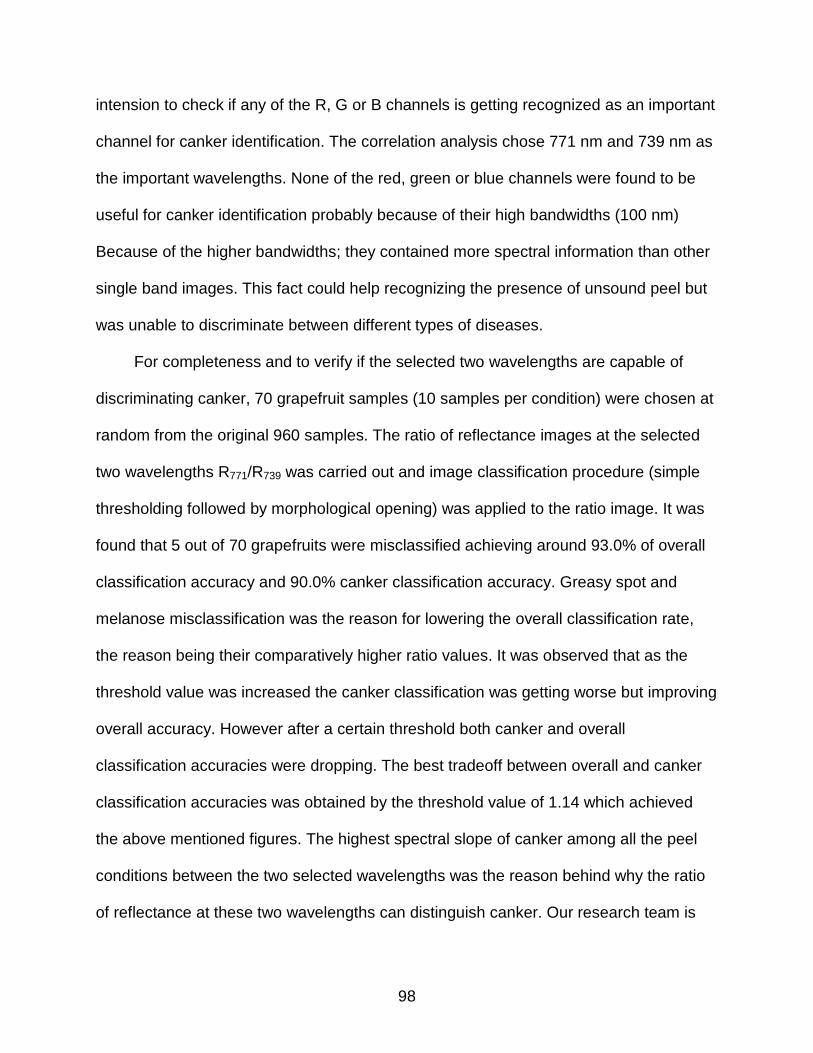
98
intension to check if any of the R, G or B channels is getting recognized as an important
channel for canker identification. The correlation analysis chose 771 nm and 739 nm as
the important wavelengths. None of the red, green or blue channels were found to be
useful for canker identification probably because of their high bandwidths (100 nm)
Because of the higher bandwidths; they contained more spectral information than other
single band images. This fact could help recognizing the presence of unsound peel but
was unable to discriminate between different types of diseases.
For completeness and to verify if the selected two wavelengths are capable of
discriminating canker, 70 grapefruit samples (10 samples per condition) were chosen at
random from the original 960 samples. The ratio of reflectance images at the selected
two wavelengths R771/R739 was carried out and image classification procedure (simple
thresholding followed by morphological opening) was applied to the ratio image. It was
found that 5 out of 70 grapefruits were misclassified achieving around 93.0% of overall
classification accuracy and 90.0% canker classification accuracy. Greasy spot and
melanose misclassification was the reason for lowering the overall classification rate,
the reason being their comparatively higher ratio values. It was observed that as the
threshold value was increased the canker classification was getting worse but improving
overall accuracy. However after a certain threshold both canker and overall
classification accuracies were dropping. The best tradeoff between overall and canker
classification accuracies was obtained by the threshold value of 1.14 which achieved
the above mentioned figures. The highest spectral slope of canker among all the peel
conditions between the two selected wavelengths was the reason behind why the ratio
of reflectance at these two wavelengths can distinguish canker. Our research team is

99
confident of achieving better classification results with higher number of samples and by
adjusting the threshold.
Figure 6-1: Representative normal and diseased peel conditions of grapefruit samples

100
Figure 6-2: Hyperspectral imaging system for reflectance image acquisition from grapefruits

101
Figure 6-3: Red, Green and Blue filter transmittance characteristics

102
Figure 6-4: Contour of correlation coefficients between two band ratios and fruit peel conditions

103
Figure 6-5: Mean reflectance spectra of grapefruits with different peel conditions
Figure 6-6: Two band Ratio images for different disease conditions. (From L to R Canker, Greasy Spot, Insect Damage, Normal, Melanose, Scab, Wind Scar)
-
10.00
20.00
30.00
40.00
50.00
60.00
70.00
80.00
Blue Re
d
713
724
734
745
755
766
776
786
797
807
818
828
839
849
860
870
881
891
902
912
922
Refle
ctan
ce (%
)
Channels / Wavelengths (nm)
Canker Greasy Spot Insect Damage Market
Melanose Scab Wind scar

104
Figure 6-7: Image classification procedure

105
Figure 6-8: Values of two band ratio between 771 and 739 nm (R771/R739) for different peel conditions
Figure 6-9: Effect of variation of threshold values on classification accuracies
Band
Rat
io V
alue
sDiseasewise Band Ratio Values
CK GS ID MK MN SB WS
Threshold = 1.14
65.00
70.00
75.00
80.00
85.00
90.00
95.00
100.00
105.00
1.120 1.130 1.140 1.150
Clas
sific
atio
n Ac
cura
cy (%
)
Threshold
Canker
Overall

106
Table 6-1: Summary of classification results
Sr. No. Disease No. of
Samples
Rule Classifier Threshold
No. of Misclassified
Classification Accuracy (%)
1 Canker 10 1.140 1* 90.00 2 Greasy spot 10 1.140 1 90.00 3 Insect damage 10 1.140 0 100.00 4 Melanose 10 1.140 3 70.00 5 Scab 10 1.140 0 100.00 6 Wind Scar 10 1.140 0 100.00 7 Market 10 1.140 0 100.00 Overall 70 5 92.86
* Represents the number of misclassified canker samples out of the total of 10 canker infected samples.

107
CHAPTER 7 COMPENSATION OF EDGE EFFECT ON IMAGES OF SPHERICAL OBJECTS DUE
TO LIGHT SOURCE – HYPERSPECTRAL IMAGING APPLICATION
Introduction
Citrus industry has been a vital source to improving the economy of the State of
Florida. Florida produces around 70% of the overall citrus supply throughout United
States. Being such a big hub in citrus industry, Florida citrus industry has proved to be a
source of income for a considerable number of Floridians. The jobs created by the citrus
industry not only include the actual citrus growth but also the peripheral areas like
fertilizer production, pest control, disease detection and elimination etc.
Among others, one of the biggest problems which Florida citrus industry is facing
is citrus canker. Canker which can spread rapidly under certain conditions and can
cause high damage, is affecting the export of citrus from Florida to canker free areas
like Europe. Citrus farms are spread over large acres and hence pest control is very
time and cost consuming as well as laborious. The solution to this problem could be
detecting canker at early stages using some automatic technique. Recently the
computer vision and machine learning technologies have been evolved as a potential
source to detect the diseases and defects on the biological and horticultural produce.
Also the hyperspectral and multispectral techniques have proven to be very effective in
automatic disease detection for the biological products like fruits and vegetables.
Essentially all these computer vision technologies include some kind of camera to
capture images of the objects which are then processed further for detection of the
defects. The distribution of light reflected by the objects and captured by the system
camera greatly depends on the position of the light source as well as the geometry of
the object. The images captured typically undergo calibration to rectify the spectral as
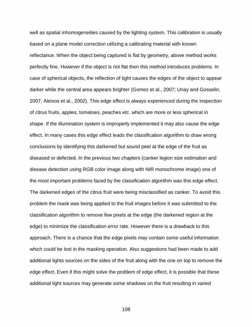
108
well as spatial inhomogeneities caused by the lighting system. This calibration is usually
based on a plane model correction utilizing a calibrating material with known
reflectance. When the object being captured is flat by geometry, above method works
perfectly fine. However if the object is not flat then this method introduces problems. In
case of spherical objects, the reflection of light causes the edges of the object to appear
darker while the central area appears brighter (Gomez et al., 2007; Unay and Gosselin,
2007; Aleixos et al., 2002). This edge effect is always experienced during the inspection
of citrus fruits, apples, tomatoes, peaches etc. which are more or less spherical in
shape. If the illumination system is improperly implemented it may also cause the edge
effect. In many cases this edge effect leads the classification algorithm to draw wrong
conclusions by identifying this darkened but sound peel at the edge of the fruit as
diseased or defected. In the previous two chapters (canker legion size estimation and
disease detection using RGB color image along with NIR monochrome image) one of
the most important problems faced by the classification algorithm was this edge effect.
The darkened edges of the citrus fruit were being misclassified as canker. To avoid this
problem the mask was being applied to the fruit images before it was submitted to the
classification algorithm to remove few pixels at the edge (the darkened region at the
edge) to minimize the classification error rate. However there is a drawback to this
approach. There is a chance that the edge pixels may contain some useful information
which could be lost in the masking operation. Also suggestions had been made to add
additional lights sources on the sides of the fruit along with the one on top to remove the
edge effect. Even if this might solve the problem of edge effect, it is possible that these
additional light sources may generate some shadows on the fruit resulting in varied

109
brightness over the fruit surface. And hence some other method has to be developed to
rectify this edge effect in case of the spherical objects to avoid misclassification.
The inappropriate lighting system can also cause the quality of the image to
deteriorate and hence it is always recommended to have as effective illumination
system as possible to avoid the costly (both monetarily and computationally)
preprocessing stages. If the illumination system is not efficient enough, it may generate
glare or shadows at particular locations of the object being photographed. It should
however be noted that it is not always possible to alter the illumination system because
of cost or other constrains. In those situations, it becomes necessary to preprocess the
images and make them suitable for further analysis by correcting the images for uniform
reflectance.
The issue of edge effect is experienced by classical computer vision system as
well as the hyperspectral imaging approach. In hyperspectral imaging technique, we
usually capture number of images of the same view at different wavelengths with a very
narrow bandwidth (approximately 10 nm). Even if the hyperspectral imaging is a lot
different than normal RGB color imaging in principle, it also uses some sort of camera
(usually EMCCD), and hence while capturing the images of a spherical object, it faces
the edge effect problem. As mentioned earlier, hyperspectral imaging is emerging as a
revolutionary technique in the field of automatic disease and defect detection on the
agricultural and horticultural products such as fruits and vegetables. However, this
technique has been reported to be very sensitive to the illumination system. Hence it
becomes necessary to eliminate the negative effects of illumination edge effect,

110
shadows or saturated regions in order to properly investigate disease defects on the
surface of a fruit.
Gomez et al. (2007) introduced a technique which considers the geometry of the
object and corrects the edge effect. They assumed the spherical object to be a
Lambertian surface and produced its digital elevation model (DEM) by predicting the
height of each pixel in the 2-D image. Uniform reflection of the light in all directions
irrespective of the direction from which it is being observed, is the inherent characteristic
of the Lambertian surface. After doing that they computed a correction factor for each
pixel by using the three coordinates (X, Y and height) of each pixel from the digital
elevation model. When this correction factor was applied to the original image, the
darkening of the edges of the spherical objects was vanished thereby equalizing the
grey level of the object surface throughout.
The overall objective of this thesis was to investigate citrus canker identification. In
this chapter of the thesis, the technique invented by Gomez et al. for edge effect
compensation was re-implemented and was applied to citrus fruits to improve the
classification rate of citrus canker by avoiding the false positive errors due to edge
blackening. Hence the objectives of this particular exploration were,
• To re-implement the algorithm designed by Gomez et al. for edge effect compensation
• To test the effectiveness of the algorithm by applying it to the citrus fruits and checking the grey level of the fruit image in different areas (edge and center)
Materials and Methods
Hyperspectral Imaging System
A hyperspectral imaging system was used to acquire reflectance images from
citrus samples. Schematic diagram of the system is illustrated in Figure 7-1. It is a push

111
broom, line-scan based imaging system that utilizes an electron multiplying charge-
coupled-device (EMCCD) camera (iXon, Andor Technology Inc., South Windsor, CT,
USA). The EMCCD has 1004×1002 pixels and is thermoelectrically cooled to -80°C
through a double-stage Peltier device. An imaging spectrograph (ImSpector V10E,
Spectral Imaging Ltd., Oulu, Finland) and a C-mount zoom lens (Rainbow CCTV H6X8,
International Space Optics, S.A., Irvine, CA, USA) are mounted to the camera. The
instantaneous field of view (IFOV) is limited to a thin line by the spectrograph aperture
slit (30 μm), and the spectral resolution of the imaging spectrograph is 2.8 nm. Through
the slit, light from the scanned IFOV line is dispersed by a prism-grating-prism device
and projected onto the EMCCD. Therefore, for each line-scan, a two-dimensional
(spatial and spectral) image is created with the spatial dimension along the horizontal
axis and the spectral dimension along the vertical axis of the EMCCD. The lighting unit
consists of two 21 V, 150 W halogen lamps powered with a DC voltage regulated power
supply (TechniQuip, Danville, CA, USA). The light is transmitted through optical fiber
bundles toward line light distributors. Two line lights are arranged to illuminate the IFOV.
A programmable, motorized positioning table (BiSlide-MN10, Velmex Inc., Bloomfield,
NY, USA) moves citrus samples (five for each run) transversely through the line of the
IFOV. One thousand seven hundred and forty line scans are required for five fruit
samples, and 400 pixels covering the scene of the fruit at each scan are saved,
generating a 3-D hyperspectral image cube with the spatial dimension of 1740×400 for
each band. However as this was just an experimental study and not many samples
were used only 700 lines were captured for two fruits saving the 3-D image containing
two fruits having dimensions 700×400 for each band. Later on while estimating the

112
geometric correction factor, the algorithm demands treating single fruit at a time and
hence the image of the two fruits was cut into two images each containing one fruit.
Spectral calibration of the system was performed using an Hg-Ne spectral calibration
lamp (Oriel Instruments, Stratford, CT, USA). Because of inefficiencies of the system at
certain wavelength regions (e.g., low light output in the visible region less than 450 nm,
and low quantum efficiency of the EMCCD in the NIR region beyond 930 nm), only the
wavelength range between 450 and 930 nm (totaling 92 bands with a spectral resolution
of 5.2 nm) was used in this investigation. The parameterization and data-transfer
interface software for the hyperspectral imaging system were developed using a SDK
(Software Development Kit) provided by the camera manufacturer on a Microsoft Visual
Basic (Version 6.0) platform in the Windows operating system.
Flat Field Correction
As mentioned in the earlier paragraph, halogen lamps (21 V, 150 W) were used for
the illumination in the hyperspectral imaging system. The problem associated with the
lighting provided by the halogen lamps is that it suffers with high order of directionality.
The above mentioned fact results in varied intensity of the light source in the plane of
the scene which is called the spatial variation of light source. In order to take care of this
issue, the flat field correction was carried out. During the procedure of the flat field
correction the image was pre-processed using a flat white panel of known reflectance.
This white panel is usually called a white reference. In this study the white Spectralon
panel was used as a reference. The first step was to perform the correction of the
hyperspectral image based on the ratio of reflectance of the fruit (ρ(λ)) and the radiance
of the light source (I(λ)) as denoted by equation (7-1).

113
R(λ) = ρ(λ)I(λ)
(7-1)
Where, R(λ) is the spatially corrected reflectance image of the fruit. However the
reflectance of the fruit (ρ(λ)) and the radiance of the light source (I(λ)) cannot be
measured as absolute values using the hyperspectral imaging system. Hence in order
to achieve this correction the white and dark references were used. Therefore the
spatial variation of the light source was rectified using the following equation:
R(λ) = Rs (λ) − Rd (λ)Rw (λ) − Rd (λ)
∗ 𝛹𝛹Ref (7-2)
Where,
λ = Wavelengths
Rs(λ) = Original (uncorrected) reflectance image of the fruit
Rd(λ) = Reflectance image of dark current
Rw(λ) = Reflectance image of white reference
𝛹𝛹Ref = Reflectance factor of the white reference panel
The dark current image Rd(λ) was acquired with the light source off and the camera lens
covered with the cap and the white reference image Rw(λ) was acquired using the white
Spectralon panel. The actual reflectance factor (𝛹𝛹Ref) of the white panel was around
98.5% in the wavelength range covered for the study (450 – 930 nm) however in this
exploration for simplicity it was assumed to be 100%. The correction mentioned in the
equation (7-2) was applied to all the monochrome images in the wavelength range
mentioned above. The relative reflectance images processed using above mentioned
procedure were then multiplied by a factor of 10,000 so as to achieve the pixel values
for resultant images in the range 0 to 10,000. This multiplication factor was applied in
order to attain the pixel value range comparable to that of the original data from the

114
hyperspectral imaging camera and also to reduce the round off errors for further data
analysis. Further details about the flat field correction can be found in Qin et al. (2008).
Image Masking and Binning
After correcting the images for spatial variation the mask for the fruit image was
created with an intention of removing the noisy background. The mask template was
formed by determining the threshold value by visual inspection of one of the
monochrome images (765 nm) that had good contrast between fruit surface and the
background. The mask was then applied to extract the fruit pixels and remove the
background from all the monochrome images in the hyperspectral image cube. The
subsequent analysis used these masked images for further processing.
Since hyperspectral image involves a large amount of data, spatial binning
technique is used for data reduction. In this process the image data is averaged by few
neighboring pixels in horizontal or vertical direction or in both directions (as per
requirement) at each wavelength. Image binning was used during first two studies but it
was not performed during the third part i.e., edge effect compensation as it was just an
experimental study. The algorithms for flat field correction as well as image masking
and binning were developed by our research team (Qin et al. 2008) during prior
explorations. For further details one can refer to Qin et al. 2008.
Derivation of Geometric Correction Factor
In order to remove the blackened edges of the image of citrus fruit due to the edge
effect and to make the intensity of the fruit surface uniform throughout, the geometric
correction was applied to the image. The expression for the geometric correction factor
(εg) was derived by starting with the illumination model. The illumination provided to the
spherical object by the light source (IT(λ)) was modeled as a function of two illumination
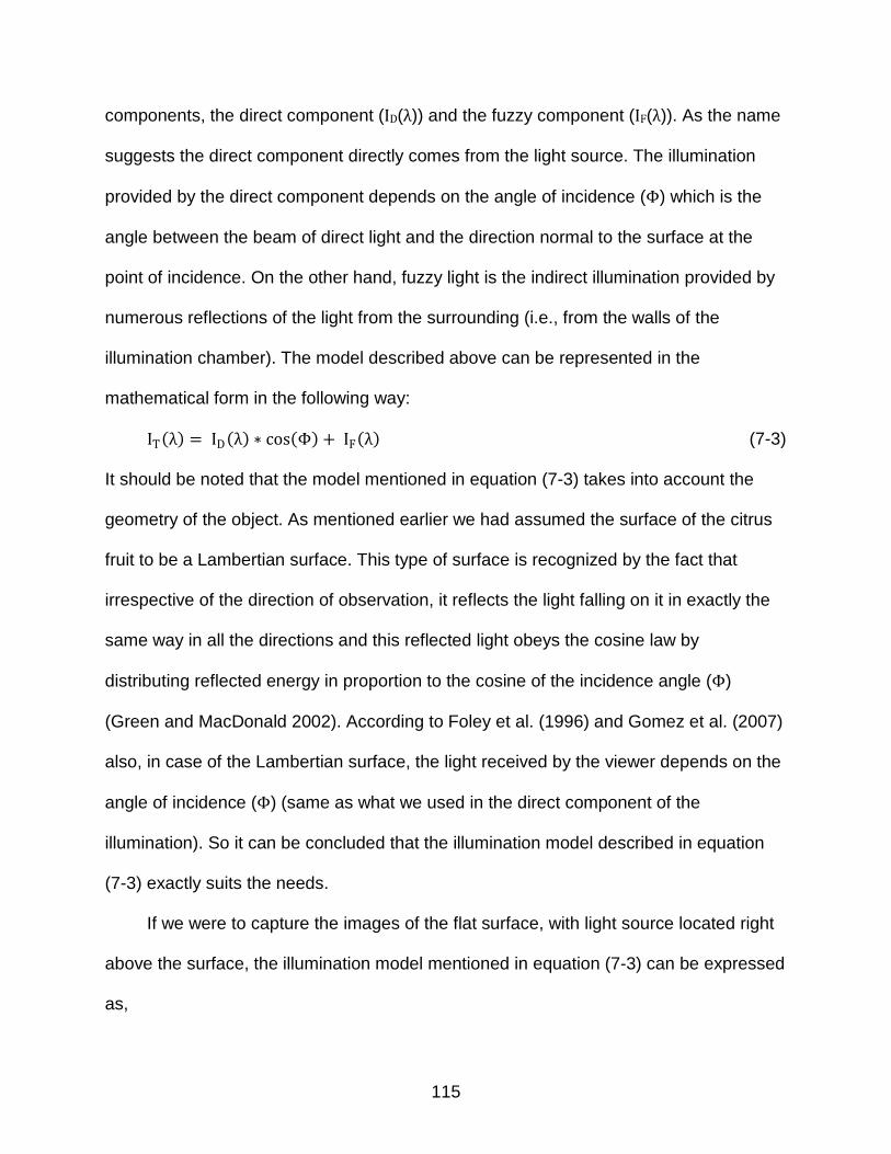
115
components, the direct component (ID(λ)) and the fuzzy component (IF(λ)). As the name
suggests the direct component directly comes from the light source. The illumination
provided by the direct component depends on the angle of incidence (Φ) which is the
angle between the beam of direct light and the direction normal to the surface at the
point of incidence. On the other hand, fuzzy light is the indirect illumination provided by
numerous reflections of the light from the surrounding (i.e., from the walls of the
illumination chamber). The model described above can be represented in the
mathematical form in the following way:
IT(λ) = ID(λ) ∗ cos(Φ) + IF(λ) (7-3)
It should be noted that the model mentioned in equation (7-3) takes into account the
geometry of the object. As mentioned earlier we had assumed the surface of the citrus
fruit to be a Lambertian surface. This type of surface is recognized by the fact that
irrespective of the direction of observation, it reflects the light falling on it in exactly the
same way in all the directions and this reflected light obeys the cosine law by
distributing reflected energy in proportion to the cosine of the incidence angle (Φ)
(Green and MacDonald 2002). According to Foley et al. (1996) and Gomez et al. (2007)
also, in case of the Lambertian surface, the light received by the viewer depends on the
angle of incidence (Φ) (same as what we used in the direct component of the
illumination). So it can be concluded that the illumination model described in equation
(7-3) exactly suits the needs.
If we were to capture the images of the flat surface, with light source located right
above the surface, the illumination model mentioned in equation (7-3) can be expressed
as,

116
I(λ) = ID(λ) + IF(λ) (7-4)
Where,
I(λ) is the total average lights which is nothing but radiance of the light source
mentioned in equation (7-1). In the present study the light source was located right
above the object being captured. Hence it should be noted that if the light source is
located right above the object, the illumination model no longer depends on the angle of
incidence (Φ). When it comes to a flat surface, the angle Φ is equal to zero for every
point on the surface, making the “cos(Φ)” term in equation (7-3) equal to one every time.
So one should keep in mind that equations (7-3) and (7-4) represent the same model
while capturing the images of a flat object. However they are potentially different models
when it comes to capturing a spherical object (provided that the light source is located
right above the object being captured).
In order to derive the expression for the geometric correction factor (εg), two
parameters, αD and αF were defined. The parameter αD was the ratio of the direct light
(ID(λ)) and the total average lights (I(λ)), while the parameter αF was the ratio between
the fuzzy light (IF(λ)) and the total average lights (I(λ)). Hence,
αD = ID (λ)I(λ)
(7-5)
And,
αF = IF (λ)I(λ)
(7-6)
Rearranging equations (7-5) and (7-6) we get,
ID (λ) = I(λ) ∗ αD (7-7)
IF(λ) = I(λ) ∗ αF (7-8)
If (7-7) and (7-8) were substituted in (7-4) we get the following identity:

117
αD + αF = 1 (7-9)
Substituting (7-7) and (7-8) in (7-3) we get the following expression.
IT(λ) = [ I(λ) ∗ αD ∗ cos(Φ)] + [I(λ) ∗ αF] (7-10)
Now rearranging equation (7-9) to get expression for αF and substituting that in equation
(7-10) we get,
IT(λ) = I(λ) ∗ [αD ∗ cos(Φ) + (1 − αD )] (7-11)
Rearranging equation (7-11) to obtain expression for I(λ) in terms of IT(λ), αD and Φ,
I(λ) = IT (λ)[αD ∗cos (Φ) + (1− αD )]
(7-12)
Substituting equation (7-12) in equation (7-1) and rearranging we get,
ρ(λ)IT (λ) = R(λ)
[αD ∗cos (Φ) + (1− αD )] (7-13)
Equation (7-13) represents the spatially as well as geometrically corrected image.
Equation (7-13) suggests that if the reflectance image of the fruit (ρ(λ)) is divided by the
illumination model which considers the spherical geometry of the fruit (IT(λ)), we achieve
the spatial and geometrical correction of the image. The expression on the right hand
side of equation (7-13) proposes that we can achieve the geometric correction of the
spatially corrected image (R(λ)) by dividing it with the factor of [αD ∗ Cos(Φ) + (1 −
αD )]. This expression represents the expression for the Geometric correction factor (εg).
Hence,
εg = [αD ∗ Cos(Φ) + (1 − αD )] (7-14)
Rewriting the equation (7-13) in terms of geometric correction factor,
ϱ(λ) = R(λ)[αD ∗Cos (Φ) + (1− αD )] = R(λ)
εg (7-15)
Where,

118
ϱ(λ) is the spatially as well as geometrically corrected image.
Gomez et al. (2007) had defined αF as the ratio between the average amount of
light (across all bands) detected by CCD (levels of grey) at the points those coincide
with the perimeter of the fruit and the total average amount of light received by the CCD
from the whole fruit. At the perimeter, as the angle of incidence (Φ) is 90 degrees, the
only component that provides lighting to the fruit is the fuzzy illumination (IF(λ)) while for
the entire fruit surface the lighting is the combination of direct (ID(λ)) and fuzzy
illumination (IF(λ)) i.e., I(λ). Gomez et al. conducted a study and plotted the value of αF
for different points on the perimeter of the clemenules mandarins and then averaged
them for each fruit to get value of αF for every fruit. Finally the mean value of αF was
computed, by taking the mean of values of αF for all the fruits, to be 0.4896. Also when
he plotted the values of αF for all the points on the perimeter of one single fruit the
values were distributed around the mean value very close to 0.4896. The mean value of
parameter αD was then calculated from equation (7-9) as 0.5104. According to the
hypothesis of Gomez et al. (2007), the parameters αD and αF are related to the
illumination system and not to the objects being captured. Hence the values of these
parameters were assumed to be constant during their entire study. In the case of our
investigation, the value of αD was not estimated through tests but it was assumed to be
a constant and equal to the mean value obtained by Gomez et al. during their studies of
mandarin (i.e., equal to 0.5104).
Generating the Digital Elevation Model
The geometric correction factor (εg) is a function of two elements, the parameter αD
which is the ratio direct lights (ID) and the total average lights (I) and the angle of

119
incidence Φ which is the angle between the beam of direct light and the direction normal
to the surface. In order to calculate the angle Φ, we need to know the Cartesian
coordinates (i.e., X, Y and heights) of each pixel of the fruit image. However, from the
2-D image of the fruits we obtain only the X and Y coordinates and not the height of any
pixel. This is precisely the reason why we generate the Digital Elevation Model (DEM).
DEM is the 3-D model of the fruit produced from the 2-D image. The basic assumption
in the process of developing this 3-D DEM is that the citrus fruits are quasi-spherical.
We can compute the geometric correction factor εg for each pixel as soon as the model
has been constructed and elevations (heights) of each of the pixels have been
estimated. However, the DEM should be developed separately for each fruit because of
the possible difference in the sizes of different fruits. The subsequent steps should be
followed to construct this DEM:
Step I – Locating the center of mass (Cg) of the fruit and determining the
interpolation network meridians: In order to locate the center of mass (Cg) of the fruit
we first need to determine the pixels that belong to the fruit and separate them from the
background i.e., to obtain the fruit mask. This mask was extracted from the image by
using an algorithm previously developed by our research team as mentioned in the
‘Image Masking and Binning’ section (Qin et al., 2008). This mask creates the black and
white binary image with white pixels (value = 1) indicating pixels belonging to fruit while
black pixels (value = 0) represent the background. Once the mask was extracted, the X
and Y locations of the pixels on the edge of the mask were identified. Now in order to
locate the center of mass, few (np) equidistant points on the edge of the mask were
selected which were called pilot points. The higher the number of pilot points selected,

120
the more accurate the location of center of mass and the more accurate end results we
can obtain. In this study we selected 30 (np = 30) pilot points on the edge. This was
done by translating the edge of the mask to the origin (0, 0) and then grabbing the (X,
Y) locations of all the pixels on the edge at an angular step of (2π / np-1). Then the
center of mass was (Cg) calculated using the equation (7-16).
Cg = 1np
∗ ∑ Pinpi=1 (7-16)
Where, Pi are the (X, Y) locations of the selected np pilot points on the edge. Now the
lines joining each of those Pi points and the center of mass (Cg) are nothing but the
meridians of interpolation network in the DEM. Figure 7-2 shows the 30 selected pilot
points (Pi) on the edge of the mask of the fruit image, which when connected with the
center of mass (Cg) forms the meridians of the interpolation network. The pilot points are
highlighted as solid circles while the center of mass is shown by a star.
Step II – Obtaining the maximum height of the fruit: To facilitate the
construction of digital elevation model (DEM) it is mandatory to obtain the height
coordinate i.e., elevation of each pixel of the fruit image. To achieve this goal, the
maximum height of the fruit was determined and then the elevations of each individual
pixels were obtained by interpolation. The maximum height of the fruit was computed
from the distance between the center of mass (Cg) and the pilot points (np) using the
equation (7-17).
hc = 1np
∗ β ∗ ∑ �CgPi�npi=1 (7-17)
Where,
�CgPi� = Distance between center of mass Cg and pilot point Pi i.e., the radius of the fruit.
β = Flattening factor.

121
As the algorithm may be sensitive to surface irregularities and may result in estimating
less spherical shape, the flattening factor was used to take into acount such
irregularities which are often found in the biological products. However in the present
study the flattening factor (β) was assumed to be one for simplicity.
Step III – Determining the elevations of the interpolation network: As
mentioned earlier the elevations of each of the image pixels were calculated using the
maximum height of the fruit (hc). But before that the nodes of interpolation and the
interpolation network need to be obtained. This was done by subdividing each of the
radii (CgPi) into few numbers of radii segments (rij) and then locating the interpolation
node at the end of each of the segments. The (XY) coordinates of all the nodes were
also determined during the process. In the segment rij, the index ‘i’ varies from 1 to np
for np number of radii (np = 30 in our case) and the index ‘j’ varies from 1 to the number
of segments. In this study we chose to divide each of the radii into 16 segments. After
determining the (XY) coordinates of the nodes, their heights (hij) were evaluated by
modeling the ellipses in the plane formed by each of the radii (CgPi) and the maximum
height (hc) of the fruit with (CgPi) and hc to be the semi axes of the ellipse in the
respective plane. The following characteristic equation of ellipse was used to compute
the heights of the nodes i.e., hij.
rij2
�Cg Pi �2 + hij
2
hc2 = 1 (7-18)
This procedure was repeated for np number of times for the np number of ellipses
formed on the np number of planes in order to compute the heights of all the nodes on
the np number of radii. Once this was done we had obtained the (X, Y, Z) coordinates

122
for all the interpolation nodes. The interpolation network for the DEM was formed by
these coordinates of all the nodes of interpolation.
Step IV – Acquiring the elevations of each pixel belonging to fruit by
interpolation: After the interpolation network was formed and the (X, Y, Z) coordinates
of all the interpolation nodes were computed, the elevations of all the intermediate
pixels of the fruit were obtained by interpolation. The MATLAB commands ‘meshgrid’
and ‘griddata’ were used for the task. The command ‘meshgrid’ was used to duplicate
the X and Y coordinates of all the pixels of the fruit image for generating the 3-D model
of the fruit. The command ‘griddata’ was used in conjunction with the (X, Y, Z)
coordinates of the interpolation nodes in order to obtain the Z or height coordinates i.e.,
elevations of all the intermediate pixels. After this was done the 3-D wireframe
parametric surface of the fruit was produced using the MATLAB command ‘mesh’. Once
the above mentioned four steps were followed the 3-D digital elevation model (DEM)
was generated, the properties of which were then used to estimate geometric correction
factor for each fruit pixel.
Estimation of Geometric Correction Factors
As derived earlier, the geometric correction factor (εg) is given by the following
equation (7-19).
εg = αD ∗ cos(Φ) + (1 − αD) (7-19)
It should be recalled that the geometric correction factor (εg) was a function of two
parameters, the parameter αD which is the ratio of direct lights (ID) and the total average
lights (I) and the angle of incidence Φ which is the angle between the beam of direct
light and the direction normal to the surface. The geometric parameters obtained from

123
the digital elevation model were exploited for estimating the value of angle Φ. The angle
Φ was calculated from the spatial coordinates of each pixel (i.e., X, Y, Z Cartesian
coordinates) as follows:
tan(Φ) = √X2+ Y2
Z (7-20)
Where, Z is the elevation of each pixel (hXY) estimated in the digital elevation model. The
geometric correction factor (εg) was estimated for each pixel using the equations (7-19)
and (7-20). The constant αD was obtained from the work of Gomez et al. (2007) as
equal to 0.5104.
After calculating the geometric correction factors (εg) for all the pixels, each pixel is
divided by the corresponding correction factor. One should note that while calculating
the center of mass (Cg) we had translated the edge of the fruit mask to the origin (0, 0).
So while applying the correction factor to each pixel one should take enough care to
divide each pixel by appropriate correction factor by properly matching the contour of
the correction factors with that of the mask.
Algorithm Validation Tests
In order to validate the edge effect compensation algorithm few tests were
conducted. A couple of market quality oranges were purchased from the supermarket
for the tests. The first experiment was carried out to prove that the same region of the
citrus fruit has similar reflectance in different areas of the image after applying the
geometric correction factor. This experiment was conducted by rotating the fruit in steps
of approximately 20 degrees and capturing the images at all the locations. The
reflectance of the same region of interest in the fruit was measured at different locations
and compared. The reflectance measurement was done using ENVI 4.3 software (ITT

124
Visual Information solutions, Boulder, CO USA). The fruits were marked with angular
graduations with step size equal to 20 degrees using a black permanent marker. Each
fruit was marked with three regions of interest, square in shape and random in size. The
images of the fruit at 0, 20 and 40 degrees were captured and the mean reflectance of
each of the region was plotted (at 0, 20 and 40 degrees) separately as the reflectance
spectra by averaging the reflectance of each pixel included in the region of interest
using ENVI 4.3. The pixels in the regions of interest were selected in the zoom window
manually, by using various drawing methods (e.g., polygon, rectangle, ellipse, point,
grow, and merge etc.). Enough care was taken while selecting the pixels to avoid the
edges of the square regions marked with the permanent marker. The reflectance
spectra of the region of interest of the fruit, before and after applying the correction
factor were compared to identify the effect of applying the correction.
The second experiment included measuring and comparing the reflectance of the
market quality orange peel at different locations before and after applying the geometric
correction factor. This was done by acquiring the reflectance spectra of the different
regions of interest of the fruit over the wavelength range for the study (450 – 930 nm)
and comparing them. The aim of this trial was to prove that the reflectance of the pixels
in different regions of the fruit equalizes or at least the difference between the
reflectance of pixels at edge and that of at the center reduces after application of the
correction. The technique similar to that of the first test was used for second test also.
The three regions of interest were selected in such a way that one was at the center
and the other two were closer to the edge. The reflectance of all the three regions of
interest at 0, 20 and 40 degrees was plotted in separate plots and compared for

125
evaluating the effect of the correction. The reflectance measurement was done in the
same way as that in the first experiment.
Results, Observations and Discussion
Digital Elevation Model Observations
The digital elevation model (DEM) was constructed in order to obtain the
geometric parameters needed to compute the geometric correction factor for each pixel.
The process was initiated by acquiring the mask of the fruit and choosing 30 pilot points
(Pi) on the edge of the mask for computing the center of mass of the fruit. The Figure
7-2 portrays the mask obtained from the fruit image along with the pilot points on the
perimeter of the mask. After the pilot points were captured, the meridians of the
interpolation network were formed by joining the center of mass (Cg) and all the pilot
points (Pi). Once the meridians are in place, the maximum height (hc) of the elevation
model of the fruit was calculated. Each meridian of the interpolation network was then
divided into 16 segments (rij) to obtain the nodes of the interpolation. Figure 7-3 shows
these interpolation nodes (green in color) on one of the meridians of the network along
with all the 30 pilot points (red in color) on the perimeter of the fruit. The elevations of all
the nodes were then computed by modeling the ellipses in the plane formed by each of
the radii (CgPi) and the maximum height (hc) of the fruit with (CgPi) and hc to be the semi
axes of the ellipse in the respective plane. One such transversal plane along with the
computed elevations of the respective nodes are demonstrated in the Figure 7-4. The
modeled ellipse with the interpolation nodes on it can be viewed from Figure 7-5 and
Figure 7-6 which are drawn in Solid Works 2009 - 2010. Figure 7-5 is a side view
(viewed from direction normal to the transversal plane in which ellipse is modeled) and
Figure 7-6 is the 3-D view of that ellipse. Figure 7-3 shows the view of Figure 7-6 taken

126
from top (i.e., top view of Figure 7-6). The interpolation network was generated as soon
as the estimation of elevations of all the nodes on all the meridians were estimated and
the (X, Y, Z) coordinates of all the nodes were determined. The construction of
interpolation network was followed by the estimation of heights of all the intermediate
pixels by interpolation. This concluded the structuring of the digital elevation model. The
digital elevation model for one of the fruits is shown in Figure 7-7.
Geometric Correction Factor Observations and Results
As noted earlier, the geometric correction factor (εg) was a function of two
elements, the parameter αD which is the ratio of direct lights (ID) and the total average
lights (I) and the angle of incidence Φ which is the angle between the beam of direct
light and the direction normal to the surface. However, as mentioned previously the
parameter αD had been assumed to have a constant value of 0.5104 that was obtained
from the work of Gomez et al. (2007) which he computed as the average value of αD for
different citrus fruit samples. So the geometric correction factor (εg) only depends on
angle of incidence Φ. The angle Φ was calculated for each pixel based on the Cartesian
coordinates of that pixel which were obtained from the digital elevation model. The
geometric correction factor for each pixel was then plotted in the XY plane to examine
its contour. Figure 7-8 shows this contour of the geometric correction factor. When an
image of the citrus fruit is captured, the top-center area of the fruit appears brightest and
as we move towards the fruit edge the image becomes darker. So when we apply the
geometric correction to the image, ideally the pixels at the center of the image should
get divided by a factor of 1 as this is the brightest region of the fruit while as we go away
from the center towards edge the geometric correction factor should have lower value.

127
Figure 7-8 supports the ideology mentioned here. The geometric correction factor had
the highest value (i.e., 1) in the central region while it was found to be decreasing
gradually towards the edge in concentric manner with minimum at edge. Also one other
point to be observed in Figure 7-8 is that the geometric correction factor of the fruit
background (i.e., the pixels of the image those don’t belong to fruit) is 1 which is logical
as these pixels need not to be corrected.
The effect of application of the geometric correction to one of the citrus samples is
shown in the Figure 7-9. The left image is the citrus fruit before application of the
geometric correction while the right one is after application of the correction. The fruit
was affected with canker and the image was captured during prior studies. The image
shown is the monochrome image at 724 nm. As can be viewed from the left image,
before applying the algorithm the image appeared brighter in the central part while the
peripheral area was darker. As discussed earlier, this was because of the spherical
geometry of the fruit which resulted in this edge effect. Clearly the image after correction
appears brighter than the one before correction. Also the brightness of the entire image
seems to have more uniformity throughout than the uncorrected image.
Validation Test Results
The first experiment was to measure and compare the reflectance of the same
region of the fruit at different orientations of the fruit, before and after applying the
geometric correction. Figure 7-10 shows one of the fruits marked with the angular
graduations and the regions of interest. The reflectance spectra of all three regions of
interest were plotted before and after application of the geometric correction. For
demonstration purposes the reflectance spectra of region of Interest 3 (ROI 3) are
shown in the Figure 7-11(A) and 7-11(B) before and after application of the geometric

128
correction factor respectively. As can be seen from Figure 7-11(A), the reflectance of
the ROI 3 at 0 and 20 degrees are pretty close to each other. However the reflectance
at 40 degrees is quite lower than the other two. One reason behind this could be the
number pixels selected in the region of interest at different angles. At 0 and 20 degrees
the pixels selected in the ROI were 385 and 367; respectively however those selected
at 40 degrees were 230. As we rotated the fruit by higher angle lesser the portion from
the ROI was visible to the camera and hence at 40 degrees a fewer number of pixel
were selected. Also it should be noted that the maximum reflectance has occurred at
around 660 nm at all three angles. The maximum reflectance at 0 degrees was around
60%, at 20 degrees it was approximately 57% and at 40 degrees it was close to 39%.
These observations make sense because as the angle of rotation was increased the
portion at top moved closer to the edge in the darkened region (which is a result of edge
effect). Now if we observe the reflectance spectra of ROI 3 after geometric correction in
Figure 7-11(B) it can be witnessed that the maximum reflectance at 0, 20 and 40
degrees is respectively 67, 65 and 49% approximately. The significant improvement in
the reflectance of the fruit image after the correction is clearly visible from the spectra.
Also the difference between reflectance of the region at different orientations can be
observed to be reduced after application of the correction. These results conclude that
the same region of the fruit had similar reflectance in different areas of the image after
subjecting it to the geometric correction proposed in the study.
The second experiment consisted of measuring and comparing the reflectance of
different regions of the fruit before and after application of the correction. As mentioned
earlier three regions were selected on the fruit image, one at center and two closer to

129
the edge. The reflectance of all three regions was measured at 0, 20 and 40 degrees.
The reflectance spectra of all three regions captured at 40 degrees rotation are shown
in Figure 7-12 for display purpose. Figure 7-12(A) shows the spectra before correction
and Figure 7-12(B) shows that after the correction was applied. Obviously the two plots
differ from one another. The spectra of the three regions before applying the correction
are quite dispersed and they portray considerably high degree of variability in spite of
being a part of the same homogeneous fruit peel. On the other hand after correction all
the spectra can be seen to be overlapping each other in Figure 7-12(B). The difference
between the reflectance of the three regions has reduced by significant amount. Also if
observed carefully the maximum reflectance of ROI 1, 2 and 3 was found to be 45, 33
and 39% at around 660 nm before correction. After the correction was applied, these
numbers increased to 51, 45 and 49%. These numbers are effective enough to highlight
the consequences of application of geometric correction. At the rotation of 40 degrees
the ROI 1 had curvature only in one direction while ROI 2 and 3 had curvature in two
directions. That was the reason behind ROI 1 having highest reflectance out of the three
regions. Also after closer examination it was observed that ROI 2 had a little mark of a
blue pen inside it. This might have caused ROI 2 to have the minimum reflectance of all.
The fruit being observed had uneven curvature in the regions 2 and 3 which also could
have contributed to the different reflectance of the regions. It was concluded after the
test that after application of the geometric correction different regions on the fruit portray
similar reflectance.
In the above experimentation all three regions represented normal peel conditions
on the same fruit belonging to the marketable class. However, the darkening edge effect

130
contrasted with the brighter central area, creating confusion in the classification
algorithm (which can be seen from the spectra in Figure 7-12(A)). The point to be noted
here is that, when applying the correction, edge effect variability within the same class
reduced significantly (refer to the spectra in Figure 7-12(B)). This fact is very important
from the point of view of an automatic segregation system as it reduces the
misclassification rate by sizeable amount, regardless of the class of peel conditions
being considered. The algorithm was implemented for correcting the monochrome
images captured by the hyperspectral imaging system, however according to the
inventor of the method, Gomez et al. (2007); the methodology can be used for any
single band images including basic three channel RGB color images.
Summary and Conclusion
Florida citrus industry is a central part of the economy of the State of Florida. It has
provided tremendous amount of employment to the residents not only in the agricultural
production areas but also related jobs like packaging, processing, shipping agri-
chemicals and so on. Florida citrus industry has been facing the threat of canker for
quite some time and the state government is continuously stressing on identifying the
diseased citrus fruits and preventing them from entering canker-free areas inside and
outside United States. The automatic disease detection systems using computer vision,
image processing and pattern recognition techniques have proven themseves to be
very effective in identifying and separating cankerous citrus fruits from other peel
conditions. One of the major concerns every computer vision system faces while
capturing the images of a spherical object is the edge effect. This edge effect may
cause the segregation algorithm to confuse between sound fruit peel and the diseases
due to darkening of the edges. A model to compensate for this edge effect was

131
implemented following the study of Gomez et al. (2007) during this course of
exploration. The algorithm assumes the fruit to be a Lambertian ellipsoidal surface. With
this assumsion a 3-D digital elevation model of the fruit was developed from its 2-D
image. The cartesian coordinates (X, Y and Z) of each pixel on the fruit surface were
determined from the digital elevation model. These coordinates were used to estimate
the geometric correction factor (εg) for each pixel. When the reflectance of each pixel
was divided by the corrosponding correction factor (εg), the image corrected for the
curvature effect of the spherical object was obtained. During the process of correction,
the value of αD from Gomez et al. (2007) was assumed, yielding excellent image
enhancement. The only disadvantage of the method is that each fruit has to be treated
separately in order to create the digital elevation model. As we can process only one
fruit at a time with this methodology, it is time consuming and thus computationally
expensive. If the algorithm is implemented in a real time online application it may
demand a considerably fast processor.
As a consequence of this geometric correction it becomes feasible to retrieve the
portion of the reflected signal that was lost while capturing an image of a spherical
object due to its curvature. We can then estimate the true reflectance that should
actually reach the camera. The correction helped to equalize the intensity of radiation
over the whole surface of the fruit and hence eliminate edge effect darkening. Additional
experiments were conducted to show that the reflectance becomes more uniform over
the fruit surface thus correcting the image for geometric variation. These results might
interest the researchers and scientists as they lead to reduced misclassification due to
edge effect.

132
Figure 7-1: Hyperspectral imaging system for reflectance image acquisition from grapefruits

133
Figure 7-2: Pilot points and center of mass
Figure 7-3: Pilot points (red in color) and nodes of interpolation (green in color) of one of the meridians

134
Figure 7-4: Transversal plane formed by maximum fruit height (hc) and center of mass of the fruit (Cg). The computed elevations of the interpolation nodes is also shown by ‘center line’

135
Figure 7-5: Side view of the modeled ellipse and the elevations of interpolation nodes
Figure 7-6: 3-D view of the modeled ellipse and the elevations of interpolation nodes

136
Figure 7-7: Digital elevation model

137
Figure 7-8: Contour of geometric correction factor (εg)
Figure 7-9: Effect of application of geometric correction – Single band image at 724 nm
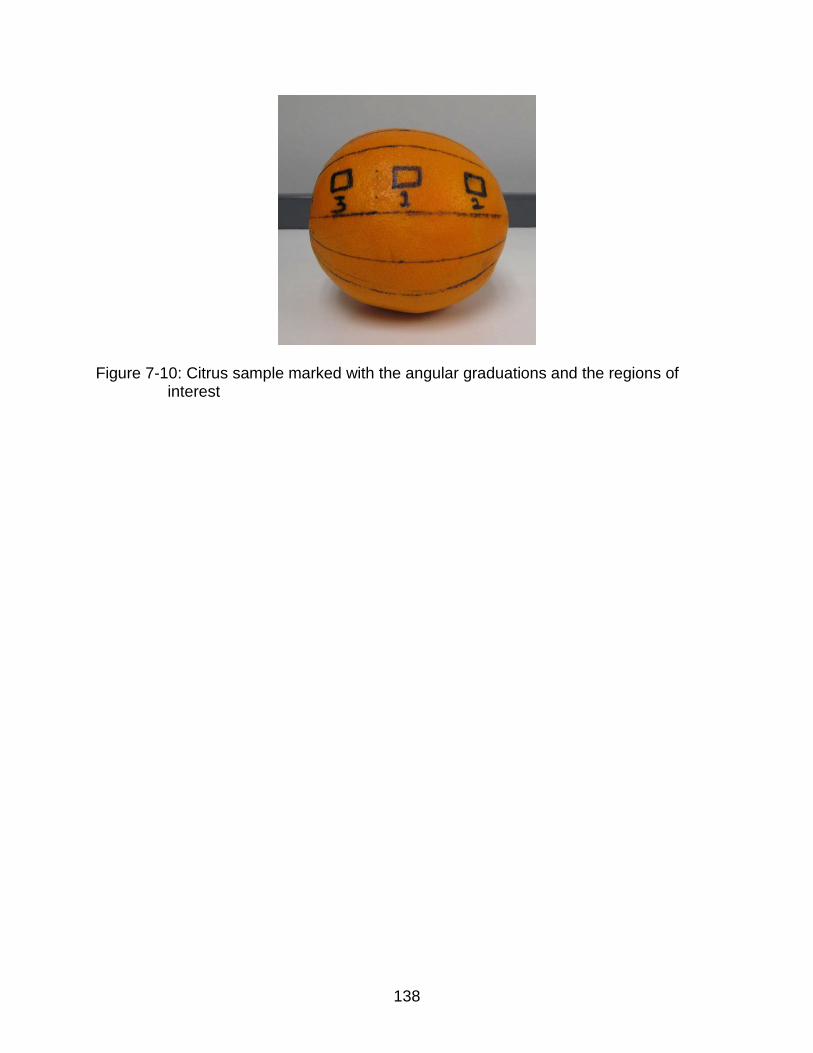
138
Figure 7-10: Citrus sample marked with the angular graduations and the regions of interest

139
(A)
(B)
Figure 7-11: Reflectance spectra of ROI 3 (A) Before applying correction (B) After applying correction
-
10.00
20.00
30.00
40.00
50.00
60.00
70.00
452
473
494
514
535
556
577
598
619
640
661
682
703
724
745
766
786
807
828
849
870
891
912
Refle
ctan
ce (%
)
Wavelengths (nm)
Uncorrected Spectra - ROI 3
0 Deg + 20 Deg + 40 Deg
-
10.00
20.00
30.00
40.00
50.00
60.00
70.00
80.00
452
473
494
514
535
556
577
598
619
640
661
682
703
724
745
766
786
807
828
849
870
891
912
Refle
ctan
ce (%
)
Wavelengths (nm)
Corrected Spectra - ROI 3
0 Deg + 20 Deg + 40 Deg

140
(A)
(B)
Figure 7-12: Reflectance spectra of all three ROIs at the rotation of 40 degrees (A) Before applying correction (B) After applying correction
-
10.00
20.00
30.00
40.00
50.00
452
473
494
514
535
556
577
598
619
640
661
682
703
724
745
766
786
807
828
849
870
891
912
Refle
ctan
ce (%
)
Wavelengths (nm)
Uncorrected Spectra at 40 Deg
ROI 1 ROI 2 ROI 3
-
10.00
20.00
30.00
40.00
50.00
60.00
452
473
494
514
535
556
577
598
619
640
661
682
703
724
745
766
786
807
828
849
870
891
912
Refle
ctan
ce (%
)
Wavelengths (nm)
Corrected Spectra at 40 Deg
ROI 1 ROI 2 ROI 3

141
CHAPTER 8 OVERALL SUMMARY, CONCLUSIONS AND FUTURE SCOPE
Summary and Conclusions
Being the second largest industry in Florida, the citrus industry represents an 8.7
billion dollars industry employing tens of thousands of employees in various related
jobs. Citrus industry has become a backbone of the economy of the State of Florida
during the last century. However citrus canker is one of the biggest challenges the
industry is facing right now as it is affecting the export of citrus fruits to several
international markets including the European countries. The State has taken
considerable amount of measures to stop the spread of the disease. The basic
underlying objective of this thesis was to develop an approach for canker detection on
the packaging line. Three different types of studies were conducted during the course of
this research.
The first study was aimed at estimating the capability of the previously developed
multispectral algorithm using correlation analysis to detect smallest possible canker
lesion on the citrus fruit. More specifically the goal of this work was to determine the
size of the smallest canker lesion that can be detected. The optimal wavelengths
selected using correlation analysis were 834 nm and 729 nm. The best overall
classification accuracy achieved was 95.7% when the binary threshold value of 1.275
was used. This threshold value was found to give best tradeoff between canker
classification and overall classification. The smallest lesion detected by the lesion size
estimation algorithm had the surface area of 2.16 sq. mm. and equivalent diameter was
1.66 mm.

142
The second part of the thesis consisted of an attempt to develop a novel approach
to discriminate citrus canker from other surface conditions. The idea was to explore if a
two camera system with one CCD color camera (to capture RGB color image) and one
monochrome camera (to capture NIR single band image) could be built for canker
detection in online real time packaging application. As this was an experimental study,
the RGB color image was simulated from the single band images in the visible range
(450-700 nm) from the previously captured hyperspectral data. The red, green and blue
channels of the RGB image were then concatenated with remaining single band images
from the hyperspectral data (700-930 nm) to generate the image for analysis. This
image was then subjected to the correlation analysis (CA) to identify the key channels.
The CA did not select any of the red, green or blue channels as a significant channel for
canker identification. The reason being higher bandwidths of the R, G and B channels
which not only might have included the information to detect canker but also other peel
conditions. It was concluded that RGB color image (along with some single band
monochrome image) cannot be utilized to discriminate canker from other peel
conditions based on simple thresholding technique.
The third and final piece of the thesis was to re-implement the compensation
algorithm to eliminate the adverse effects of light source while capturing the image of
spherical objects like citrus fruits. The motivation behind this study was to reduce the
misclassification of citrus fruits due to the edge blackening effect which our research
team had been facing. The algorithm was developed by Gomez et al. 2007. The image
was corrected for the spatial variations caused by intensity of light source as well as
geometrical variation caused by the spherical geometry of the citrus fruit. The spatial

143
correction which commonly known as “flat field correction” was achieved with the help of
a white panel of known reflectance. The geometric correction was accomplished by
constructing a 3-D digital elevation model (DEM) of the fruit from its 2-D image. This
DEM provided us with the geometric properties of the fruit like X, Y, and Z coordinates
which were exploited in the course of estimating the geometric correction factor for each
pixel. The corrected image portrayed improved and uniform brightness of the citrus fruit
surface throughout. Few tests were also conducted to validate the results of the
algorithm.
Future Scope
The basic limitation of all the three explorations was all of them were developed for
the laboratory based study. The most important future step would be to adapt these
algorithms for rapid real time online packaging applications. The RGB + NIR images
were subjected to simple binary threshold based classification approach. The
prospective work might include some texture based studies for canker discrimination.
Also if such texture based algorithm works the next challenge would be to tune the
algorithm for processing the citrus fruits for canker detection in the real time
applications.
The edge effect compensation algorithm seemed to work absolutely fine during
these laboratory based studies. However it was observed that the algorithm takes quite
some time to process the 3-D hyperspectral image data of high resolution. Also each
fruit had to be treated separately during the geometric correction estimation process. So
the basic challenge is to minimize the processing time of the algorithm. Also the future
work might include processing more than one fruit at a time. The algorithm will be fine

144
tuned and implemented on the packaging conveyor available with the research team to
demonstrate its applicability for the real time applications.

145
APPENDIX A MATLAB CODE FILES - ESTIMATION OF DETECTION LIMIT FOR SIZE OF CITRUS
CANKER LESIONS BASED ON HYPERSPECTRAL REFLECTANCE IMAGING
%% Program to compute the Number of pixels in the smallest canker lesion %% and to find the (X, Y) coordinates of the center of that lesion clear all; clc; close all; K = 0.6; % mm/pixel (pixel resolution) a = K^2; % area of one pixel n = 1; %% Finding the Number of Pixels in smallest canker lesion % org_img = Final Binary image obtained during the Image Classification method org_img = imread('fruit30_final_binary.tif'); level = graythresh(org_img); org_img_binary = im2bw(org_img,level); for i = 1:200 post_img = bwareaopen(org_img,n); if (max(max(abs(post_img - org_img_binary))))==0 n= n+1; elseif (max(max(abs(post_img - org_img_binary))))==1 break end % The Equivalent area of the legion : A = (n-1) * a; % disp('Sq mm'); end % subplot(2,1,1); imshow(org_img_binary); % subplot(2,1,2); imshow(post_img); % Number of Pixels in smallest lesion N = n-1 A; %% Finding the Coordinates of the center of the smallest lesion L = bwlabeln(org_img); [L_row, L_col] = size(L); area = regionprops(L, org_img, 'Area'); ctr = regionprops(L, org_img, 'Centroid'); z = []; ctr_smallest = []; for i = 1:length(area)

146
if (area(i).Area) < n z = [z, i]; ctr_smallest = [ctr_smallest; ctr(i).Centroid]; end end ctr_smallest %% End

147
APPENDIX B MATLAB CODE FILES - DETECTION OF CITRUS CANKER USING RGB COLOR
IMAGE ALONG WITH NIR MONOCHROME IMAGES
Main Program File
Simulation of the RGB + NIR images
clear all; clc; close all; % Loading the Input file address = 'C:\Nikhil\Nikhil_Office Comp Back up (Jan 5 2010)\1 Nikhil\Research\Hyper Demo for Duke\10 samples of each condition\Norm_R_RG_SB_SC_002'; [image_hyper,p,t] = hsi_read (address); [row, col, band] = size(image_hyper); %% Building the R, G, B Filters and Creating the Filtered Red, Green & Blue channel images % 1} Green (G) Filter x1 = sort([603.3800 598.1500 592.9200 587.6800 582.4500 577.2200 571.9900 566.7600 561.5300 556.3000 551.0700 545.8400 540.6000 535.3700 530.1400 524.9100 519.6800 514.4500 509.2200 503.9900 498.7500]); avg1 = 550; std_dev1 = sqrt(1/(length(x1)-1)*sum((x1 - avg1).^2)); % "y1" = Green Filter (Gussian Approximation) y1 = (1/(sqrt(2*pi*std_dev1^2))) * (exp(-((x1 - avg1).^2)/(2*std_dev1^2))); % Normalizing y1 to have its values between 0 to 1 y1 = y1*80; % Applying the Filter m1 = length(x1); for i = 1:m1 T = image_hyper(:, :, (m1-i+1)); % T = Image at perticular wavelength g = T.*y1(i); % Adding the Filtered images at each wavelength to the 3rd dimension to % create "green" channel gr(:,:, i) = g; end % Averaging the Green channel to create a grayscale (green) image green = sum(gr,3)/length(x1); % 2} Blue (B) Filter w = [];

148
z = 451.67-5.23; for l=1:200 if z <= 400 break; else z=z-5.23; w = [w, z]; end end x2 = sort([503.9900 498.7500 493.5200 488.2900 483.0600 477.8300 472.6000 467.3700 462.1400 456.9100 451.6700 w]); avg2 = 450; std_dev2 = sqrt(1/(length(x2)-1)*sum((x2 - avg2).^2)); % "y2" = Blue Filter (Gussian Approximation) y2 = (1/(std_dev2*sqrt(2*pi))) * (exp(-((x2 - avg2).^2)/(2*std_dev2^2))); % Normalizing y2 to have its values between 0 to 1 y2 = y2*81; % Applying the Filter m2 = (length(x2)-length(w)); for j = 1:m2 T2 = image_hyper(:, :, (m2-j+1)); % T = Image at perticular wavelength b = T2.*y2(j+length(w)-1); % Adding the Filtered images at each wavelength to the 3rd dimension to % create "blue" channel bl(:, :, j) = b; end % Averaging the Blue channel to create a grayscale (blue) image blue = sum(bl,3)/length(x2); % 3} Red (R) Filter x3 = sort([702.7700 697.5400 692.3100 687.0800 681.8500 676.6100 671.3800 666.1500 660.9200 655.6900 650.4600 645.2300 640.0000 634.7700 629.5300 624.3000 619.0700 613.8400 608.6100 603.3800 598.1500]); avg3 = 650; std_dev3 = sqrt(1/(length(x3)-1)*sum((x3 - avg3).^2)); % "y3" = Red Filter (Gussian Approximation) y3 = (1/(sqrt(2*pi*std_dev3^2))) * (exp(-((x3 - avg3).^2)/(2*std_dev3^2))); % Normalizing y3 to have its values between 0 to 1 y3 = y3*80; % Applying the Filter m3 = length(x3); for k = 1:m3 T = image_hyper(:, :, (m3-k+1)); % T = Image at perticular wavelength r = T.*y1(k); % Adding the Filtered images at each wavelength to the 3rd dimension to % create "red" channel

149
re(:,:, k) = r; end % Averaging the Red channel to create a grayscale (red) image red = sum(re,3)/length(x3); % % Displaying Red, Green & Blue grayscale images side by side % figure; % subplot(1,3,1); imshow(mat2gray(red)); % subplot(1,3,2); imshow(mat2gray(green)); % subplot(1,3,3); imshow(mat2gray(blue)); % Combining Red, Green & Blue grayscale images to create RGB color image color = cat(3, 0.4*red, 0.5* green, 0.1*blue); % figure; % imshow(mat2gray(color)); % % Plotting the R, G, B filter Characteristics figure; plot(x1,y1, '--g','LineWidth',2); grid on; hold on; plot(x2,y2, '--b','LineWidth',2); hold on; plot(x3,y3, '--r','LineWidth',2); band17 = image_hyper(:, :, 17); band39 = image_hyper(:, :, 39); %% Combining the RGB color image with the remaining NIR single band images % S is and array containing all the images (concatenated in the 3rd dimension) to be considered for Correlation Analysis S = cat(3, color, image_hyper(:, :, 1:43)); S = single(S); hsi_write(S,'RGB_NIR_SB_002.img'); %% End
Generation of Spectra of Different Disease Conditions
clear all; clc; close all; %% Generation of CK and Non-CK spectra % Loading all the Spectra files in ASCII format load('RGB_NIR_CK_Spectra_001.txt'); load('RGB_NIR_CK_Spectra_002.txt'); load('RGB_NIR_GS_Spectra_001.txt'); load('RGB_NIR_GS_Spectra_002.txt'); load('RGB_NIR_ID_Spectra_001.txt'); load('RGB_NIR_ID_Spectra_002.txt');

150
load('RGB_NIR_MK_Spectra_001.txt'); load('RGB_NIR_MK_Spectra_002.txt'); load('RGB_NIR_MN_Spectra_001.txt'); load('RGB_NIR_MN_Spectra_002.txt'); load('RGB_NIR_SB_Spectra_001.txt'); load('RGB_NIR_SB_Spectra_002.txt'); load('RGB_NIR_WS_Spectra_001.txt'); load('RGB_NIR_WS_Spectra_002.txt'); spectra_ck = [RGB_NIR_CK_Spectra_001(:, 2:6), RGB_NIR_CK_Spectra_002(:, 2:6)]; spectra_ck = spectra_ck'; spectra_nck = [RGB_NIR_GS_Spectra_001(:, 2:6), RGB_NIR_GS_Spectra_002(:, 2:6), RGB_NIR_ID_Spectra_001(:, 2:6), RGB_NIR_ID_Spectra_002(:, 2:6), RGB_NIR_MK_Spectra_001(:, 2:6), RGB_NIR_MK_Spectra_002(:, 2:6), RGB_NIR_MN_Spectra_001(:, 2:6), RGB_NIR_MN_Spectra_002(:, 2:6), RGB_NIR_SB_Spectra_001(:, 2:6), RGB_NIR_SB_Spectra_002(:, 2:6), RGB_NIR_WS_Spectra_001(:, 2:6), RGB_NIR_WS_Spectra_002(:, 2:6)]; spectra_nck = spectra_nck'; a = [927.71,922.48,917.25,912.02,906.79,901.55,896.32,891.09,885.86,880.63,875.40,870.17,864.94,859.70,854.47,849.24,844.01,838.78,833.55,828.32,823.09,817.86,812.62,807.39,802.16,796.93,791.70,786.47,781.24,776.01,770.78,765.54,760.31,755.08,749.85,744.62,739.39,734.16,728.93,723.69,718.46,713.23,708]; wl = [943.4, 938.17, 932.94, a]; % Saving the Spectra files in MATLAB format save('data_ca_spectra_ck_nck.mat', 'spectra_ck', 'spectra_nck', 'wl'); %% End
Function Files
Function to Perform the Correlation Analysis on the Image Data
function hsi_ca % calculate the correlation coefficient between a spectral wavelength pair combination and the disease condition (0=normal, 1=defect). % Reference: Correlation analysis of hyperspectral imagery for multispectral wavelength selection for detection of defects on apples, % Sens. & Instrumen. Food Qual. (2008) 2:90-96 load data_ca_spectra_ck_nck; band = 1:46; num_band = size(band,2); % wavelength num_sample1 = size(spectra_ck,1); % canker num_sample2 = size(spectra_nck,1); % non-canker % wavelength ratios ratio_spectra_ck = zeros(num_band,num_band,num_sample1); % 2-band selection ratio_spectra_nck = zeros(num_band,num_band,num_sample2);

151
for k = 1:num_sample1 for i = 1:num_band for j = 1:num_band ratio_spectra_ck(i,j,k) = spectra_ck(k,i)/spectra_ck(k,j); % 2-band selection, I1/I2 end end end for k = 1:num_sample2 for i = 1:num_band for j = 1:num_band ratio_spectra_nck(i,j,k) = spectra_nck(k,i)/spectra_nck(k,j);% 2-band selection, I1/I2 end end end index = [ones(1,num_sample1) zeros(1,num_sample2)]; % disease condition (0=normal, 1=defect) A = zeros(1, num_sample1); B = zeros(1, num_sample2); corr_ratio = zeros(num_band,num_band); for i = 1:num_band for j = 1:num_band for k1 = 1:num_sample1 A(k1) = ratio_spectra_ck(i,j,k1);%2-band selection end for k2 = 1:num_sample2 B(k2) = ratio_spectra_nck(i,j,k2);%2-band selection end corr_matrix = corrcoef([A B],index); corr_ratio(i,j) = corr_matrix(1,2); end end % save corr_coeff_2_band corr_ratio figure; axes('FontSize',14); contourf(wl,wl,corr_ratio); % contourf(band,band,corr_ratio) colorbar ('FontSize',14); axis equal axis tight title('Contour of Correlation Coefficients', 'FontSize',16); xlabel('Wavelengths (nm)', 'FontSize',16); ylabel('Wavelengths (nm)', 'FontSize',16); %[V1 L1] = max(corr_ratio); [V1 L1] = max(abs(corr_ratio)); [ratio_max column1] = max(V1); row1 = L1(column1);

152
ratio_max band1 = row1 band2 = column1 %% End
Function to Read the Image File in ENVI Format in MATLAB
function [image_hyper,p,t] = hsi_read (fname) % Reads an image of ENVI standard type to a [col x line x band] MATLAB array % SYNTAX % image_hyper=hsi_read(fname) % [image_hyper,p]=hsi_read(fname) % [image_hyper,p,t]=hsi_read(fname) % % INPUT : % fname string giving the full pathname of the ENVI image to read. % % OUTPUT : % image_hyper: c by l by b array containing the ENVI image values organised in c : cols, l : lines and b : bands. % p: 1 by 3 vector that contains (1) the number of cols, (2) the number of lines and (3) the number of bands of the opened image. % % t: string describing the image data type string in MATLAB conventions. % % NOTE : % hsi_read needs the corresponding image header file generated % automatically by ENVI. The ENVI header file must have the same name as % the ENVI image file + the '.hdr' exention. tic; % Parameters initialization elements={'samples ' 'lines ' 'bands ' 'data type '}; d={'bit8' 'int16' 'int32' 'float32' 'float64' 'uint16' 'uint32' 'int64' 'uint64'}; % Check user input if ~ischar(fname) error('fname should be a char string'); end % Open ENVI header file to retreive s, l, b & d variables rfid = fopen(strcat(fname,'.hdr'),'r'); % Check if the header file is correctely open if rfid == -1 error('Input header file does not exist'); end; % Read ENVI image header file and get p(1) : number of samples, % p(2) : number of lines, p(3) : number of bands and t : data type while 1 tline = fgetl(rfid);

153
if ~ischar(tline), break, end [first,second]=strtok(tline,'='); switch first case elements(1) [f,s]=strtok(second); p(1)=str2num(s); case elements(2) [f,s]=strtok(second); p(2)=str2num(s); case elements(3) [f,s]=strtok(second); p(3)=str2num(s); case elements(4) [f,s]=strtok(second); t=str2num(s); switch t case 1 t=d(1); case 2 t=d(2); case 3 t=d(3); case 4 t=d(4); case 5 t=d(5); case 12 t=d(6); case 13 t=d(7); case 14 t=d(8); case 15 t=d(9); otherwise error('Unknown image data type'); end end end fclose(rfid); t=t{1,1}; % Open the ENVI image and store it in the 'image' MATLAB array disp([('Reading '),(num2str(p(1))),(' cols x '),(num2str(p(2))),(' lines x '),(num2str(p(3))),(' bands') (' of type '), (t), (' hyperspectral image...')]); fid=fopen(strcat(fname,'.img')); image_hyper_array=fread(fid,t); image_hyper=reshape(image_hyper_array,[p(1),p(3),p(2)]); image_hyper=permute(image_hyper, [3 1 2]); fclose(fid); Time_Used_In_Minute = round (toc/60) %% End

154
Function to Write the MATLAB Array into an Image File in ENVI Format
function i=hsi_write(image,fname) % Write a MATLAB array to a file in ENVI standard format from a [col x line x band] array % % SYNTAX % % hsi_write(image, fname) % % INPUT : % % % image c by l by b name of the MATLAB variable containing the array to export to an ENVI image, with c = cols, l the lines and b the bands % fname string full pathname of the ENVI image to write. % Parameters initialization im_size=size(image); im_size(3)=size(image,3); elements={'samples =' 'lines =' 'bands =' 'data type ='}; d=[4 1 2 3 12 13]; % Check user input if ~ischar(fname) error('fname should be a char string'); end cl1=class(image); % if cl1 == 'double' % img=single(image); % else % img=image; % end img=image; cl=class(img); switch cl case 'single' t = d(1); case 'int8' t = d(2); case 'int16' t = d(3); case 'int32' t = d(4); case 'uint16' t = d(6); case 'uint32' t = d(7); otherwise error('Data type not recognized'); end

155
wfid = fopen(fname,'w'); if wfid == -1 i=-1; end % disp([('Writing ENVI image ...')]); fwrite(wfid,img,cl); fclose(wfid); % Write header file fid = fopen(strcat(fname,'.HDR'),'w'); if fid == -1 i=-1; end fprintf(fid,'%s \n','ENVI'); fprintf(fid,'%s \n','description = {'); fprintf(fid,'%s \n','Exported from MATLAB}'); fprintf(fid,'%s %i \n',elements{1,1},im_size(1)); fprintf(fid,'%s %i \n',elements{1,2},im_size(2)); fprintf(fid,'%s %i \n',elements{1,3},im_size(3)); fprintf(fid,'%s %i \n',elements{1,4},t); fprintf(fid,'%s \n','interleave = bsq'); fclose(fid); %% End

156
APPENDIX C MATLAB CODE FILES - COMPENSATION OF EDGE EFFECT ON IMAGES OF
SPHERICAL OBJECTS DUE TO LIGHT SOURCE
Main Program File
clear all; clc; close all; % Loading the Input file load('C:\Nikhil\Nikhil_Office Comp Back up (Jan 5 2010)\Research\Edge effect compensation-final folder\data_hyper_citrus_canker_original.mat');%%%% mask1 = extract_mask ('data_hyper_citrus_canker_original', 'data_dark_white_reference'); [mask1_row, mask1_col] = size(mask1); %% Obtaining all the pixels (xy) on the Edge of the mask mask_edge = double(edge(mask1)); np = 30; % np = Number of points to be selected on the Periphery of the mask xy = []; n = 0; for i=1:mask1_row for j=1:mask1_col if mask_edge(i,j) == 1 n=n+1; xy = [xy [i j]']; end end end xy = xy'; [xy_row, xy_col] = size(xy); cp = mean(xy); %% Obtaining the array of "np" number of equidistant Pilot points on the periphery of the mask xy = xy - ones(size(xy,1),1)*cp; % Transforming all points to the origin np_xy = []; step = 2*pi/(np-1); for th = -pi : step : pi, for i=size(xy,1):-1:1, %disp([th i]) nn = abs(th - atan2(xy(i,2),xy(i,1))); if nn<.009 np_xy = [np_xy; xy(i,:)]; xy(i,:)=[]; break end end end

157
np_xy1 = np_xy + ones(size(np_xy,1),1)*cp; %% Obtaining the Center of mass (cg) of the mask cg = (1/np) * sum(np_xy); cg1 = (1/np) * sum(np_xy1); % Plotting the center of mass & Pilot Points on the edge of mask figure; imshow(mask1); hold on; axis equal; plot(np_xy1(:,2),np_xy1(:,1),'o', 'MarkerFaceColor','b','MarkerSize',7); hold on; plot(cg1(:,2),cg1(:,1),'*', 'MarkerSize',10); title('Pilot Points and the Center of mass', 'FontSize',12); %% Obtaining the Maximum height of the fruit & the Elevations of the Interpolation network num = 16; % num = Number of points to be considered on each Radius. beta = 1; % beta = Flattening factor sum1 = 0; radmat = []; hij = []; for i = 1: size(np_xy) rad = norm(np_xy(i,:) - cg); radmat = [radmat; rad]; sum1 = sum1 + rad; end % Obtaining Maximum height (hc) of fruit hc = (1/np) * beta * sum1; % Obtaining the X, Y & Z coordinates of the Nodes of interpolation for m = 1 : size(np_xy) dm = radmat(m); d = np_xy(m, :); theta = atan2(d(2), d(1)); xyz = []; for rij = 0 : (dm/(num - 1)) : dm x = rij * cos(theta); y = rij * sin(theta); h = sqrt((1-(rij/dm)^2)*hc^2); xyz = [xyz; [x y h]]; end xyz_mat{m} = xyz; end xyz_mat1 = xyz_mat'; xyz_cat = []; for i = 1:(length(xyz_mat1)) xyz_cat = vertcat(xyz_cat, xyz_mat1{i}); end %% Obtaining the Heights for all the pixels by interpolation (Z value for each of the in between pixel)

158
tix = -139.5:1:139.5; tiy = -164:1:164; %%%%%%% [XI,YI] = meshgrid(tix,tiy); ZI = griddata(xyz_cat(:,1),xyz_cat(:,2),xyz_cat(:,3),XI,YI); for i=1:length(ZI(:)), if isnan(ZI(i)), ZI(i)=0; end; end % Displaying the Digital Elevation Model (DEM) figure; mesh(XI,YI,ZI) colorbar; axis equal; title('Digital Elevation Model', 'FontSize',13); xlabel('X Pixels','FontSize',13); ylabel('Y Pixels', 'FontSize',13); zlabel('Elevation Pixels', 'FontSize',13); % axes('FontSize',14); colorbar ('FontSize',13); % Obtaining the X, Y, & Z for all the image pixels in a Single column. x_all = []; y_all = []; z_all = []; xyz_all = []; for i = 1 : (size(YI,1)) for j = 1 : (size(XI,2)) x_all = [x_all; XI(1,j)]; y_all = [y_all; YI(i,1)]; z = ZI(i,j); if isnan(z) z = 0; end; z_all = [z_all; z]; end end xyz_all = [x_all, y_all, z_all]; %% Calculation of Geometric Correction Factor (epci) alphaD = 0.5104; % Mean value of alphaD fi_all = []; epci_all1 = []; % Calculation of Angle of Incidence for i=1:(size(xyz_all,1)) x = xyz_all(i,1); y = xyz_all(i,2); z = xyz_all(i,3); if z == 0 epci = 1; epci_all1 = [epci_all1; epci]; elseif z ~= 0 temp = (sqrt((x^2) + (y^2))) / z; fi = atan(temp); fi_all = [fi_all; fi];

159
% Calculation of gemetric correction factor epci = (alphaD * cos(fi)) + (1 - alphaD); epci_all1 = [epci_all1; epci]; end end % Reshaping the matrix "epci_all" (Matrix of Geometric Correction factor for all the pixels) to the Image dimensions. epci_2d = reshape(epci_all1, mask1_row, mask1_col); epci_edge = double(edge(epci_2d)); % figure; imshow(epci_edge); %% Matching the contour of the Fruit image and contour of geometric correction factor C1 = conv2(mask_edge,epci_edge,'same'); %figure,surf(C1) [val,I] = max(C1); [val,I2] = max(val); Xidx = I2; Yidx = I(I2); C2 = conv2(mask_edge,mask_edge,'same'); %figure,surf(C2) [val,I] = max(C2); [val,I2] = max(val); Xidx2 = I2; Yidx2 = I(I2); Xshift = Xidx2 - Xidx; Yshift = Yidx2 - Yidx; % Shifting the contour of Geometric correction factor to match the Fruit contour epci_2d = circshift(epci_2d, [Yshift, Xshift]); % Plotting the Contour of the geometric correction factor figure; imagesc(epci_2d); colorbar; colormap jet; axis equal; set(gca,'CLim', [0.5, 1.0]); title('Contour of Geometric Correction Factor', 'FontSize',13); xlabel('X Pixels','FontSize',13); ylabel('Y Pixels', 'FontSize',13); colorbar; % Applying the Geometric correction factor the the image epci_all = reshape(epci_2d, mask1_row*mask1_col, 1); a = size(R_sample, 1)*size(R_sample, 2); for p = 1:size(R_sample,3) R_sample_masked(:,:,p) = R_sample(:,:,p) .* mask1; R_temp = reshape(R_sample_masked(:,:,p), a, 1); R_temp_corrected = R_temp ./ epci_all; R_sample_corrected(:,:,p) = reshape(R_temp_corrected, size(R_sample, 1), size(R_sample, 2)); end

160
% Plotting the Fruit image (724 nm) before and after geometric correction figure; title('Effect of Geometric Correction', 'FontSize',13); subplot(1,2,1); imshow(mat2gray(R_sample_masked(:,:,40))); xlabel('Before Correction', 'FontSize',13) subplot(1,2,2); imshow(mat2gray(R_sample_corrected(:,:,40))); xlabel('After Correction', 'FontSize',13) %% End
Function Files
%% Function to extract the mask of the fruit image function [R_mask] = extract_mask (filename_sample, filename_reference) % Generate mask for hyperspectral reflectance images % Example: R_mask = extract_mask ('data_hyper_citrus_canker_original', 'data_dark_white_reference'); % Image normalization load (filename_sample); load (filename_reference); band_mask = 42; num_scan = size(R_sample, 1); R_dark_mono = repmat(mean(R_dark(:,:,band_mask)), num_scan, 1); R_white_mono = repmat(mean(R_white(:,:,band_mask)), num_scan, 1); R_mask = uint16(10000*(R_sample(:,:,band_mask) - R_dark_mono)./ (R_white_mono - R_dark_mono)); clear R_sample R_dark R_white; % Mask generation level_mask = 0.005; R_mask_original = double(R_mask); R_mask = im2bw(R_mask, level_mask); R_mask = bwareaopen(R_mask, 4000, 8); R_mask = double(imfill(R_mask, 'holes')); R_sample_masked = R_mask_original .* R_mask; % % Plot result % figure, % subplot(2,3,1), imshow(R_mask_original, []); title ('Original Image', 'FontWeight', 'bold'); % subplot(2,3,2), imshow(R_mask, []); title ('Mask Template', 'FontWeight', 'bold'); % subplot(2,3,3), imshow(R_sample_masked, []); title ('Masked Imge', 'FontWeight', 'bold'); % subplot(2,3,4), plot([1:size(R_mask,1)], R_mask_original(:, (size(R_mask,2)-1)/2), [1:size(R_mask,1)], R_sample_masked(:, (size(R_mask,2)-1)/2), 'r'); % legend('Original','Masked'); title ('Y Profile', 'FontWeight', 'bold'); % subplot(2,3,[5 6]), plot([1:size(R_mask,2)], R_mask_original(size(R_mask,1)/2, :), [1:size(R_mask,2)], R_sample_masked(size(R_mask,1)/2, :), 'r'); % legend('Original','Masked'); title ('X Profile', 'FontWeight', 'bold');

161
% save (filename_sample, 'R_mask', '-append'); %% End

162
LIST OF REFERENCES
Aleixos, N., Blasco, J., Navarrón, F., Moltó, E., 2001. Multispectral inspection of citrus in real-time using machine vision and digital signal processors. Computers and Electronics in Agriculture. 33 (2002) 121–137.
Bishop, C. M.,2006. “Pattern Recognition and Machine Learning”. First Edition.
Cheng, X., Chen, Y. R., Tao, Y., Wang, C. Y., Kim, M. S., Lefcourt, A. M., 2004. A novel integrated PCA and FLD method on hyperspectral image feature extraction for cucumber chilling damage inspectaion. Information and Electrical Technologies Division of ASAE. ISSN 0001–2351. Vol. 47(4): 1313–1320.
Chen, Y. R., Chao, K., Kim, M. S., 2002. Machine vision technology for agricultural applications. Computers and Electronics in Agriculture. 36(2002) 173–191.
Duda, R. O., Hart, P. E., Stork, D. G., 2004. “Pattern Classification”. Second Edition.
Das, A. K., 2003. Citrus canker – A review. J. Appl. Hort. 5(1): 52–60.
Florida Statistics Site [Internet], USDA's National Agricultural Statistics Service (US); Update: 2007 June; Accessed on December 2009. Available at: http://www.nass.usda.gov/Statistics_by_State/Florida/Publications/Broc/index.asp
Foley, J., Feiner, A., Van Dam, S., Hughes, J., 1996. “Computer Graphics: Principles and Practice.” Second Edition.
Gómez-Sanchis, J., Molto´, E, Camps-Valls, G, Go´mez-Chova, L, Aleixos, N, Blasco, J. Automatic correction of the effects of the light source on spherical objects. An application to the analysis of hyperspectral images of citrus fruits. J. Food Eng 85 (2008) 191–200.
Gonzalez, R., Woods, R., Editions, S., 2004. “Digital image processing using MATLAB”.
Green, P., MacDonald, L., 2002. “Colour Engineering – Achieving Device Independent Color”. First Edition.

163
Hodge, A., E. Philippakos, D. Mulkey, T. Spreen, and R. Muraro. 2001. Economic impact of Florida's citrus industry, Extension Digital Information Source (EDIS) FE307. Gainesville, Fla.: University of Florida, Department of Food and Resource Economics, 1999–2000.
James A. Jacobs. 1994. Cooperative in the U.S. Citrus Industry, Agricultural Economist, U.S. Department of Agriculture, Rural Business and Cooperative Development Service, RBCDS Research Report 137, December, 1994.
Kim, M. S., A. M. Lefcourt, K. Chao, Y. R. Chen, I. Kim, and D. E. Chan. 2002. Multispectral detection of fecal contamination on apples based on hyperspectral imagery: Part I. Application of visible and near-infrared reflectance imaging. Trans. ASAE 45(6): 2027–2037.
Kim, M. S, Y. R. Chen, P. M. Mehl 2001. Hyperspectral reflectance and fluorescence imaging system for food quality and safety ASAE ISSN 0001–2351.
Kim, M. S., A. M. Lefcourt, Y. R. Chen, I. Kim, D. E. Chan, and K. Chao. 2002. Multispectral detection of fecal contamination on apples based on hyperspectral imagery: Part II. Application of hyperspectral fluorescence imaging. Information and Electrical Technologies Division of ASAE. ISSN 0001–2351. Vol. 45(6): 2039–2047.
Kim, D. G., Burks, T. F., Qin, J., Bulanon, D. M., 2009. Classification of grapefruit peel diseases using color texture feature analysis. Int. J. Agric. & Biol. Eng., 2009; 2(3): 41–50.
Koschan, A., Abidi, M., 2008. “Digital Color Image Processing”, First Edition.
Lee, K., S. Kang, S. R. Delwiche, M. S. Kim, and S. Noh. 2008. Correlation analysis of hyperspectral imagery for multispectral wavelength selection for detection of defects on apples. Sens. Instrum. Food Qual. Saf. 2(2): 90–96.
Lu, R., 2008. Quality evaluation of fruit by hyperspectral imaging. Chapter in “Computer vision technology in food quality evaluation” edited by Da-Wen Sun.
Lu, R. 2002. Detection of bruises on apples using Near-Infrared hyperspectral imaging. Information and Electrical technologies Division of ASAE ISSN 0001–2351. Vol. 46(2): 523–530.

164
Noordam, Jacco C., Willie HAM van den Broek, Lutgarde MC Buydens, 2005. Detection and classification of latent defects and diseases on raw French fries with multispectral imaging. Journal of the Science of Food and Agriculture 85:2249–2259 (2005) DOI: 10.1002/jsfa. 2226.
Park, B., Lawrence, K. C., W. R. Windham, R. J. Buhr 2002. Hyperspectral imaging for detecting fecal and ingesta contaminants on poultry carcasses ASAE ISSN 0001–2351.
Park, B., Chen, Y. R., Nguyen, M., 1997. Multispectral image analysis using neural network algorithm for inspection of poultry carcasses. J. Agric. Engng. Res. (1998) 69, 351–363.
Park, B., Chen, Y. R., 2000. Co-occurrence matrix texture features of multispectral images on poultry carcasses. J. Agric. Engng. Res. (2001). 78(2), 127–139.
Pydipati, R., Burks, T. F., Lee, W. S., 2005. Statistical and neural network classifiers for citrus disease detection using machine vision. Information and Electronics Technologies Division of ASAE. ISSN 0001–2351. Vol. 48(5): 2007–2014.
Pydipati, R., T. F. Burks, and W. S. Lee. 2006. Identification of citrus disease using color texture features and discriminant analysis. Comput. Electron. Agri. 52(1–2): 49–59.
Piron, A., Leemans, V., kleynen, O., Lebeau, F. Destain, M. –F., 2007. Selection of the most efficient wavelength bands for discriminating weeds from crop. Computer and Electronics in Agriculture 62 (2008) 141–148.
Palmer, M. Regents Professor at Dept of Botany of Oklahoma State University. Web document. Accessed on December 2009. Available at: http://ordination.okstate.edu/PCA.htm
Qin, J., T. F. Burks, M. S. Kim, K. Chao, and M. A. Ritenour. 2008. Citrus canker detection using hyperspectral reflectance imaging and PCA-based image classification method. Sens. Instrum. Food Qual. Saf. 2(3): 168–177.
Qin, J., T. F. Burks, M. A. Ritenour., and W. G. Bonn. 2009a. Detection of citrus canker using hyperspectral reflectance imaging with spectral information divergence. J. Food Eng. 93(2): 183–191.

165
Qin, J., T. F. Burks, Xuhui Zhao, N. P. Niphadkar and M. A. Ritenour. 2009b. Hyperspectral band selection for citrus canker detection using multispectral algorithms ASABE Paper No. 096144. Reno, Nevada: ASABE.
SAS customer support website. Copyright 2010 SAS Institute Inc. Accessed on January 2010. Available at: http://support.sas.com/publishing/pubcat/chaps/55129.pdf.
Schubert, T. S., Miller, J. W., 2000. Bacterial citrus canker. FDACS, Division of plant industry, Gainesville, Florida. 6 fold.
Shirai, Y., Kondo, N., Fujiura, T., 1998. Machine vision. Chapter in “Robotics for bioprodction systems” edited by Kondo, N., Ting, K. C.
The Imaging Source: Manufacturer of industrial machine vision cameras. How color cameras work? Web document. Accessed on January 2010. Available at: http://www.theimagingsource.com/downloads/howcolcamswp.en_US.pdf
Unay, D., Gosselin, B. 2006. Stem and calyx recognition on ‘Jonagold’ apples by pattern recognition. Journal of Food Engineering 78 (2007) 597–605.
Wikipedia – The free encyclopedia. Updated in December 2009. Accessed on Jaunary 2010. Available at: http://en.wikipedia.org/wiki/Principal_component_analysis

166
BIOGRAPHICAL SKETCH
Nikhil Pramod Niphadkar was born in 1983 in Dhule of State of Maharashtra in
India. He graduated with a Diploma in Mechanical Engineering (DME) in May 2002 from
Cusrow Wadia Institute of Technology. He earned his Bachelor of Engineering (BE)
degree in mechanical engineering in May 2005 from University of Pune, India. He
worked with John Deere Equipments Pvt. Ltd., Pune, India from Aug 2005 to August
2006 as a Graduate Trainee where he was a part of transmission manufacturing cycle
time reduction team. From November 2006 to June 2007, he worked as an Automation
Engineer at Siddheshwar Industries Pvt. Ltd., Pune, India, where he was responsible for
designing fixtures for cost efficiency and operator safety. He started his graduate
studies at University of Florida as a concurrent masters’ student in the Mechanical and
Aerospace Engineering and Agricultural and Biological Engineering Departments in
August 2007. He joined the Agricultural Robotics and Mechatronics group (ARMg) in the
Department of Agricultural and Biological Engineering where he worked as a Research
Assistant of Dr. Thomas F. Burks.