Detection and Visualization of Performance Variationsto Guide Identification of Application Bottlenecks

Matthias Weber, Ronald Geisler, Tobias Hilbrich, Matthias Lieber,Ronny Brendel, Ronny Tschuter, Holger Brunst, and Wolfgang E. Nagel

Center for Information Services and High Performance ComputingTechnische Universitat Dresden, Germany

{matthias.weber, tobias.hilbrich, matthias.lieber, ronny.tschueter, holger.brunst, wolfgang.nagel}@tu-dresden.de

Abstract—The identification of performance bottlenecks inparallel applications is a challenging task. Without some formof performance measurement tool, this task lacks any guidanceand purely relies on trial-and-error. At the same time, data setsfrom parallel performance measurements are often large andoverwhelming. We provide an effective solution to automati-cally identify and highlight several types of performance criticalsections in an application run. Our approach first identifiestime dominant functions of an application that are subsequentlyused to analyze runtime imbalances throughout the applicationrun. We then present the resulting runtime variations in anintuitive visualization that guides the analyst to performancehot spots. We demonstrate the effectiveness of our approachin a case study with three applications, detecting performanceproblems and identifying their root-causes in all cases.

I . I N T R O D U C T I O N

Today’s High Performance Computing (HPC) systemsfeature complex architectures that require software adaptionand tuning to run codes efficiently. In this regard performanceanalysis of parallel applications presents a challenging task.The analysis process involves measurements to gather datafor performance evaluation. Existing measurement suitesoffer different levels of detail. Measurements with lowlevels of detail record coarse-grain measurement samples thatare averaged across application processes. Highly detailedmeasurements provide many measurement samples and retainall individual measurement points. The latter is well-suitedto detect performance problems that vary across processes orover time, as well as to highlight root causes for several typesof performance problems. While performance measurementtools exist to capture such detailed data at scale [5], [9],the analysis of such detailed measurement data remainschallenging.

Existing analysis approaches either provide automaticsearch methods for specific problems [6], [21] or leavethe analysis task completely to the analyst and provide avisualization of the data [3], [10], [13]. While automaticsearch methods are limited to certain types of problems,pure visualization approaches cover the widest range ofpossible detectable performance problems. This makes visualanalysis methods powerful and compelling. At the sametime they suffer from a more user driven identification of

the performance problems. We provide a new approachfor visualization-based performance analysis that identifiesperformance hotspots of an application execution.

Ideally, applications making use of structured parallelismshould exhibit a regular runtime behavior throughout thecomplete run and across all processes. Meaning, that forinstance the duration of iterations should be similar betweenprocesses as well as from the beginning to the end of theapplication. If some parts of an application run slower thanthe other parts, this might indicate a performance problem.We refer to such a situation with the terms runtime imbalanceor performance variation. With our approach we detect suchimbalances and highlight areas in an application run thatexhibit notably higher runtime than others. Our performancemeasurement data sets are so-called program traces, whichare time-sorted records of timestamped application behavior.Examples for performance relevant behavior include enteringor leaving a function or sending a message from one processto another. In a parallel application, each processing elementcan create one such trace. To detect slow performing partswe first automatically identify time-dominant functions ofan application. These functions are most suitable to detectruntime imbalances. To guide the analyst, we then analyzeand visualize execution time variations of these functioninvocations throughout the application run. Applying ourapproach on top of established trace visualization methodsallows analysts to benefit from the full potential of theunderlying analysis system, as to detect the root cause of aperformance problem. In summary our approach highlightsperformance critical parts during an application execution,and thus, guides the analyst directly to performance problems.

Our contribution includes:• A method to automatically identify time-dominant func-

tions of an application run;• A scheme to calculate runtime imbalances using time-

dominant functions to reveal performance critical areas;• A visualization of runtime imbalances in a trace visu-

alizer, thus, ultimately guiding analysts to performanceproblems; and

• An application study with three examples to showcasethe effectiveness of our approach.

The remainder of this paper is organized as follows. InSection II we describe related work. Sections III-VI highlightour overall approach and methodology. In these sections wedetail how we identify and visualize runtime imbalances.In the case study in Section VII we verify the validity ofour approach for the detection of performance problems.We analyze several trace data sets and detect differentperformance problems and identify their root cause.

I I . R E L AT E D W O R K

A wide range of parallel performance analysis approachesexists. We provide an overview of their basic techniques andrelate them to our approach.

Parallel profilers like TAU [2] and HPC Toolkit [1] showaggregated statistics of an application run. Such profiles arewell suited for an overview of the performance behaviorof an application. But due to aggregation, the detection ofruntime imbalances and small slow sections can be hard oreven impossible.

Trace viewers like Vampir [3], Paraver [17], and the IntelTrace Analyzer [10] visualize performance traces to guide theuser to potential performance problems. Usually, summaryinformation provides the guidance that allows the analystto find interesting spots in timeline charts that visualizethe overall trace data. Since these tools present full datasets, they can detect runtime imbalances and bottlenecks.However, due to the large amount of data, analysts may easilymiss performance problems during their analysis. To providescalable visualization, Mohror et al. [13] propose a techniqueto compare event streams of processes. The approach takesstructurally equal processes and compares their temporalbehavior. If the temporal behavior of these processes issufficiently similar, only one representative is stored tosimplify the visualization. However, by basing the analysis ononly a few representative processes, performance problemsmay easily be hidden. Additionally, root causes, such as highinter-process communication latency on a specific process,may not be included in the selected representatives.

Weber et al. [20] propose metrics to compare traces usingalignment techniques. These techniques highlight perfor-mance differences between different application runs. At thesame time, the approach fails to highlight differences betweenprocesses inside a single run. An extension of the Paravertools suite [7] targets a tool that characterizes computationphases. It clusters these periods with a common clusteringalgorithm. The result is a classification of phases that differ ininstructions-per-second rates. While this approach providesan overview of the different performance characteristics ofcomputation phases, it does not highlight individual variationswithin processes.

A range of performance tools also employ automaticanalysis techniques for performance problems. Scalasca [21]automatically searches trace data for a range of inefficiencypatterns. Located patterns are ranked by their severity and

foobar

int foo(){ int a; a = 1 + 1;

bar();

a = a + 1; return a;}

t0 1 2 3 4 5 6

Inclusive time of foo: t = 6.

Exclusive time of foo: t = 4.

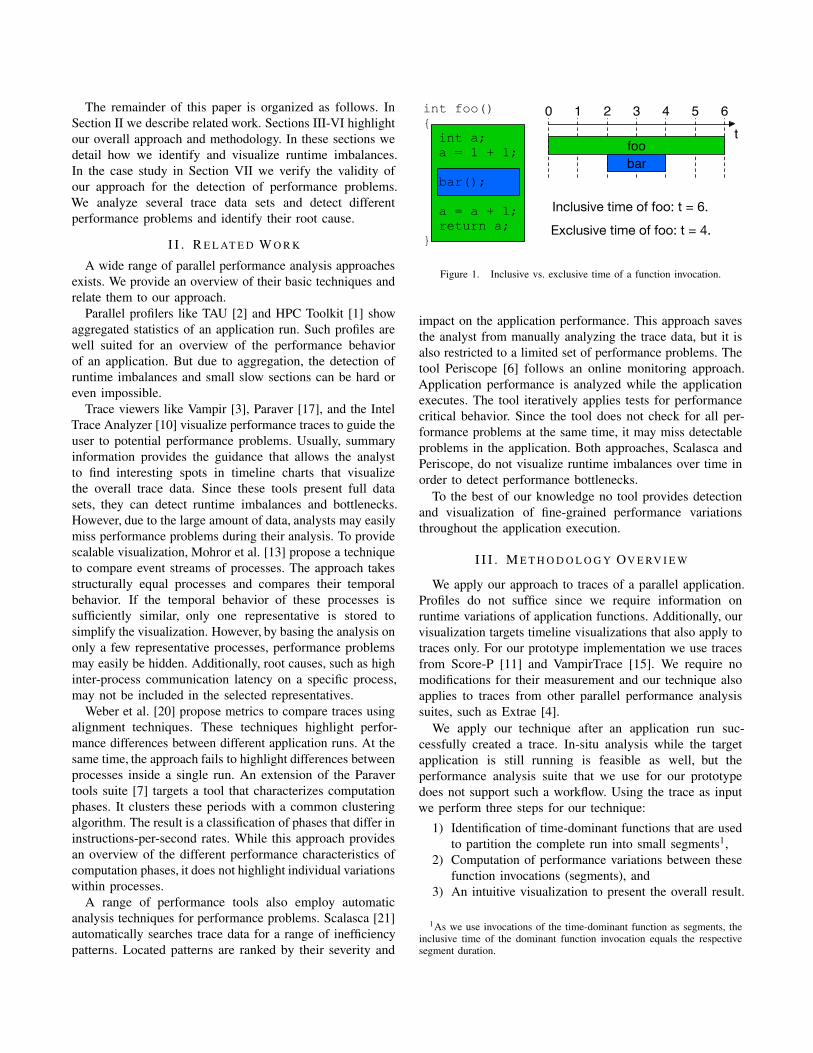
Figure 1. Inclusive vs. exclusive time of a function invocation.

impact on the application performance. This approach savesthe analyst from manually analyzing the trace data, but it isalso restricted to a limited set of performance problems. Thetool Periscope [6] follows an online monitoring approach.Application performance is analyzed while the applicationexecutes. The tool iteratively applies tests for performancecritical behavior. Since the tool does not check for all per-formance problems at the same time, it may miss detectableproblems in the application. Both approaches, Scalasca andPeriscope, do not visualize runtime imbalances over time inorder to detect performance bottlenecks.

To the best of our knowledge no tool provides detectionand visualization of fine-grained performance variationsthroughout the application execution.

I I I . M E T H O D O L O G Y OV E RV I E W

We apply our approach to traces of a parallel application.Profiles do not suffice since we require information onruntime variations of application functions. Additionally, ourvisualization targets timeline visualizations that also apply totraces only. For our prototype implementation we use tracesfrom Score-P [11] and VampirTrace [15]. We require nomodifications for their measurement and our technique alsoapplies to traces from other parallel performance analysissuites, such as Extrae [4].

We apply our technique after an application run suc-cessfully created a trace. In-situ analysis while the targetapplication is still running is feasible as well, but theperformance analysis suite that we use for our prototypedoes not support such a workflow. Using the trace as inputwe perform three steps for our technique:

1) Identification of time-dominant functions that are usedto partition the complete run into small segments1,

2) Computation of performance variations between thesefunction invocations (segments), and

3) An intuitive visualization to present the overall result.

1As we use invocations of the time-dominant function as segments, theinclusive time of the dominant function invocation equals the respectivesegment duration.

t70 1 2 3 4 5 8 9 10 11 12 13 14 15 16 17 186

bb

b

aProcess 0:

amain

b bcc

ac

i

a amain

b bcc

ac

i

a amain

b bcc

ac

i

Process 1:

Process 2:

Figure 2. For our performance variation analysis we select one time-dominant function. The selected function needs to have a possibly high inclusivetime and an invocation count higher than the number of processes. In this example function a fulfills these criteria.

I V. I D E N T I F I C AT I O N O F T I M E - D O M I N A N TF U N C T I O N S

We need to identify reoccurring parts of an applicationin order to detect performance variations during the ap-plication run. Reoccurring parts allow us to separate anoverall execution into multiple segments. Afterwards, wecan compare runtimes between the segments. Thus, the firststep of our analysis is a selection of suitable segments tohighlight performance variations. Since parallel applicationsusually execute functions repeatedly, as they are being calledin loops, we select such a function for our segments. Notethat the measurement systems that we use also supportinstrumentation of loop bodies. If such an instrumentationis in use, we can use loop bodies as well. For simplicitywe use the term function in the following. To decide whichparticular function we select as segments, we consider theirinclusive times.

When measuring a function’s invocation, there are twooptions to report the function’s duration: inclusive andexclusive time. Figure 1 depicts the difference betweeninclusive and exclusive time. Inclusive time represents thecomplete duration of a function’s invocation, from initiallyentering to finally leaving the function call. This time alsoincludes the time spent in sub-functions. The inclusive timefor function foo in Figure 1 starts with entering foo (t = 0)and stops when foo is left (t = 6). The inclusive timeincludes the sub-call to function bar and is 6 in the example.The exclusive time, on the contrary, represents only theamount of time spent directly inside the respective function’sinvocation, excluding sub-functions. The exclusive time offunction foo in Figure 1 starts with entering foo at t = 0,excludes the sub-call of function bar (t = 2 to t = 4), and

ends with leaving of foo at t = 6, i.e., it is 4 in the example.We consider inclusive time to detect dominant functions,

since it includes the overall performance impact of a function.Figure 2 illustrates an example that uses three processes andthe functions main, i, a, b, as well as c. A time-dominantfunction should have a considerable impact on the totalapplication runtime. For that we consider the aggregatedinclusive time of each function. Selecting the function withthe highest aggregated inclusive time, however, is not a goodchoice for a dominant function. In the example, this wouldbe the function main (54 time steps). Such top call-levelfunctions may be suitable to compare the runtime betweenprocesses, but they are not suited to analyze variations overthe runtime. Additionally, they provide no segmentation ofthe overall runtime. Thus, just maximum aggregated inclusivetime is not a good selection criteria alone.

As a consequence, for a time-dominant function we selecta function with high aggregated inclusive time, but whichalso features a higher number of invocations. In the exampleof Figure 2, the function with the highest inclusive time shareis main. The function main is called three times on thethree processes in total. Thus, top call-level functions likemain have exactly as many invocations as there are paral-lel processing elements. Thus, we define a time-dominantfunction f as:

• For p processing elements, f is invoked at least 2ptimes and there exists no other function that satisfiesthis condition and has higher aggregated inclusive time.

In the example, the function with the second highestinclusive time share is a (36 time steps). Function a is callednine times on three processes, i.e., it satisfies the invocationcount restriction. Hence, a is the time-dominant function forthe example.

t70 1 2 3 4 5 8 9 10 11 12 13 14 15 16 17 186

2

aProcess 0:

amain

a amain

amain

Process 1:

Process 2:

a

a

calc MPI

a

a

Process 0: 6

6

6

Process 1:

Process 2:

Process 0:

Process 1:

Process 2:

3

3

3

5

5

5

MPI

MPI

calc

calc

MPI

MPI

MPIcalc

calc

calc MPI

MPI

MPIcalc

calc

calc

5

3

1

2

2

4

1

3

1

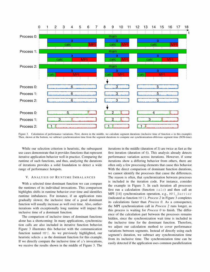
Figure 3. Calculation of performance variations. First, shown in the middle, we calculate segment durations (inclusive time of function a in this example).Then, shown at the bottom, we subtract synchronization time from the segment durations to compute our synchronization-oblivious segment time (SOS-time).

While our selection criterion is heuristic, the subsequentuse cases demonstrate that it provides functions that representiterative application behavior well in practice. Comparing theruntime of such functions, and thus, analyzing the durationsof iterations provides a solid foundation to detect a widerange of performance hotspots.

V. A N A LY S I S O F R U N T I M E I M B A L A N C E S

With a selected time-dominant function we can comparethe runtimes of its individual invocations. This comparisonhighlights shifts in runtime behavior over time and identifiesruntime imbalances. For instance, if an application runsgradually slower, the inclusive time of a good dominantfunction will usually increase as well over time. Also, outlier-iterations with exceptionally long runtime will impact theinclusive time of a dominant function.

The comparison of inclusive times of dominant functionsalone has a shortcoming: In many applications, synchroniza-tion calls are also included in iterative function behavior.Figure 3 illustrates this behavior with the communicationfunction named MPI. As we previously highlighted, ourheuristic selects a as the dominant function for this example.If we directly compare the inclusive time of a’s invocations,we receive the results shown in the middle of Figure 3. The

iterations in the middle (duration of 3) are twice as fast as thefirst iteration (duration of 6). This analysis already detectsperformance variation across iterations. However, if someiterations show a differing behavior from others, there areoften only a few processing elements that cause this behavior.With the direct comparison of dominant function durations,we cannot identify the processes that cause the differences.The reason is often, that synchronization between processesis included in the iteration code. For instance, considerthe example in Figure 3. In each iteration all processesfirst run a calculation (function calc) and then call anMPI [14] synchronization operation, e.g., MPI_Barrier(indicated as function MPI). Process 2 in Figure 3 completesits calculations faster than Process 0. As a consequence,the MPI synchronization call in Process 2 runs longer, asthis process is waiting for Process 0 to finish. The differ-ence of the calculation part between the processes remainshidden, since the synchronization wait time is included inthe inclusive time for the dominant function. Therefore,we adjust our calculation method to cover performancevariations between segments. Instead of directly using eachsegment’s duration, we subtract any synchronization timefrom its inclusive time. The synchronization time can beeasily detected if the application uses common parallelization

libraries like MPI [14], OpenMP [16], or similar. In suchcase, we check each segment for synchronization operations,e.g., MPI_Wait, MPI_Reduce, or omp barrier, andsubtract their runtime from the inclusive time of our dom-inant functions. We refer to this adapted segment time assynchronization-oblivious segment time (SOS-time) and useit as measure for runtime imbalances. Figure 3 (bottom)depicts this process for the example. Our SOS-times correctlyreflect the performance differences between the processes.For instance, for the first iteration in Figure 3 the SOS-timeof Process 2 shows 1 compared to a SOS-time of 5 forProcess 0, i.e., it highlights the computational load imbalancein the first iteration.

V I . V I S U A L I Z AT I O N O F R U N T I M E I M B A L A N C E S

As the last step of our approach, we visualize our SOS-times to the analyst. Therefore, we implemented our analysismethods in the Vampir performance analysis framework [3].To achieve an intuitive visualization, we overlay commonlyused timeline views of Vampir. We use the SOS-times asvalues for a new metric counter. For our visualization we en-code the metric with a color-coded scale. Blue—cold—colorsindicate short durations, whereas red—hot—colors indicatelong durations. Figures 4(b), 5(b), 5(c), and 6(b) in thesubsequent section present examples of our visualization.

V I I . C A S E S T U D Y

In this section we demonstrate the applicability of ourapproach with three use cases. To initially measure applica-tion performance data we use traces from the Score-P [11]and VampirTrace [15] measurement frameworks. As we il-lustrated in the methodology overview, our approach requiresno modifications at measurement time. We implement ouranalysis as part of the Vampir [3] analysis and visualizationtoolkit. In the following, we analyze trace files with knownperformance problems to demonstrate the capabilities of ourtechnique.

A. Load Imbalance - COSMO-SPECS

The first case study is an analysis of the execution ofa weather forecast code [8]. The code couples two models,COSMO and SPECS, for a more accurate simulation of cloudand precipitation processes. COSMO is the regional weatherforecast model originally developed at the German WeatherService (DWD). SPECS is a detailed cloud microphysicsmodel developed at the Leibniz Institute for TroposphericResearch (IfT). SPECS computes detailed interactions be-tween aerosols, clouds, and precipitation.

Figure 4(a) shows the Vampir timeline visualization ofthe overall application run. The execution under study uses100 MPI processes that Vampir each represents with ahorizontal bar. The colors then identify the currently activefunctions across the overall execution time. Red identifiesMPI activities, purple SPECS activities, green COSMO

activities, and yellow highlights the coupling between thetwo models. Compared to COSMO, the SPECS calculationsare significantly more compute intensive. Therefore, purpleareas—SPECS code—dominate the application run. Theexecution of COSMO code—green areas—is barely visiblein Figure 4(a). This behavior is caused by the computationaldemand of the underlying physics. However, Figure 4(a) alsoshows another trend. Throughout the execution, the fractionof MPI—red areas—increases, up to a point where MPIactivities are dominating towards the end of the run. Ourheuristic selects a dominant function whose occurrencesrepresent individual iterations. If we compare the plaininclusive time of this function (segment durations), weobserve gradually increased durations towards the end ofthe application run.

To find the cause of the degrading performance, we useour synchronization-oblivious segment time (SOS-time) fromSection III. Figure 4(b) presents this metric and highlightsthat only a few processes (Process 44, 45, 54, 55, 64, 65)exhibit increases in this metric. Particularly Process 54 needsmore time than any other process for its calculations.

The reason for this behavior is a static decomposition ofthe computational grid. COSMO employs a two dimensional(horizontal) decomposition into M ×N domains and appliesno dynamic load balancing. SPECS uses the same data struc-tures and decomposition as the COSMO model, but insteadcomputes cloud microphysics. During the execution, SPECSintroduces large load imbalances, since its computationalcost heavily depends on the presence and size distribution ofvarious cloud particle types in the grid cell [12]. Thus, thelayout of clouds in the application domain determines thelocal work. In other words, while Process 54 still performscloud microphysics calculations, the other processes idlewhile waiting for it to finish. A solution to this performanceproblem is to introduce dynamic load balancing for theSPECS model.

Our analysis and visualization correctly represents theperformance situation of the application. By following thehigh—red—values the analyst is pointed directly to the causeof the performance bottleneck.

B. Process Interruption - COSMO-SPECS+FD4

In this case study we analyze an extended version ofthe previous weather forecast code [8]. In this version thedeveloper has added a dynamic load balancing mechanism,called FD4 [12], to the SPECS model. As described inthe first case study, the high computational demand ofthe SPECS code, combined with its high dependence onlocal workload—presence of cloud particles in the domain—demand a dynamic load balancing for efficient computation.

The application run under study uses 200 MPI processes.Our initial analysis—not shown—detected that only a fewiterations behaved differently and exhibited larger durationsthan other iterations. The goal of this study is to detect the

(a) Timeline visualization of COSMO-SPECS running on 100 processes, showing increasing MPI durations (red areas) over time.

(b) Runtime variation analysis result. Several processes (middle) exhibit higher runtimes (SOS-time) in their dominant function.

Figure 4. Analysis of the COSMO-SPECS weather forecast code. (a) shows the timeline visualization. (b) shows our analysis results.

(a) Timeline visualization of COSMO-SPECS+FD4 running on 200 processes.

(b) Coarser runtime variation analysis result (SOS-time). Especially Process 20 exhibits a highduration in its dominant function.

(c) Finer runtime variation analysis result (SOS-time). Using smaller segments sizes allows directidentification of the one function invocation that causes the performance degradation.

Figure 5. Analysis of a COSMO-SPECS+FD4 application run. Displayed is just one iteration. (a) shows the timeline visualization. (b) (coarser segments)and (c) (finer segments) show our variation analysis results using SOS-time.

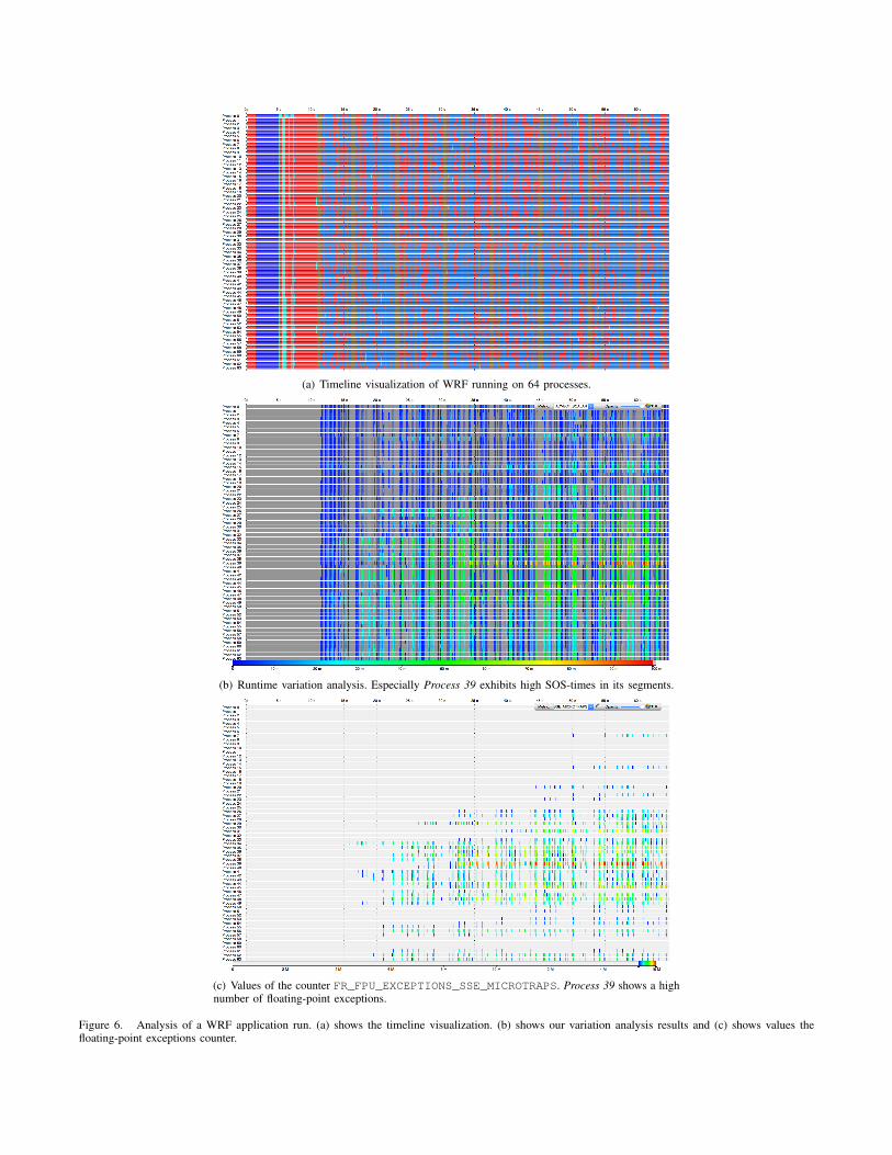
(a) Timeline visualization of WRF running on 64 processes.

(b) Runtime variation analysis. Especially Process 39 exhibits high SOS-times in its segments.

(c) Values of the counter FR_FPU_EXCEPTIONS_SSE_MICROTRAPS. Process 39 shows a highnumber of floating-point exceptions.

Figure 6. Analysis of a WRF application run. (a) shows the timeline visualization. (b) shows our variation analysis results and (c) shows values thefloating-point exceptions counter.

reason for these slow iterations. Therefore, the analyst useda second measurement run to only record slow iterations.For normal iterations the analyst discarded the tracing data.We show the timeline visualization of one slow iteration inFigure 5(a). Again, different colors represent different activitytypes. Red relates to MPI code, blue indicates areas whereperformance data was dropped, while orange and white areasrelate to SPECS activities. The black lines indicate MPImessages sent from one process to another. The runtimesof COSMO and FD4 are so short compared to SPECS thatthese areas are not directly visible in Figure 5(a). Looking atthe behavior in Figure 5(a), we see that one SPECS timestepnear the end of this iteration takes significantly longerthan the others. Especially, increased MPI wait time—morered areas—and higher message transfer times—longer blacklines—indicate this behavior. However, the reason causingthe slower timestep in this iteration is not immediatelyvisible.

By using our runtime variation analysis, we can guide theanalyst to the cause of this performance problem. We showthe result of our analysis in Figure 5(b). The red line in thefigure highlights a high SOS-time for Process 20. Thus, theperformance problem is caused by longer computation timeof Process 20. To find the exact place of the performanceproblem, we can refine granularity by adapting the dominantfunction. By choosing a function with a smaller inclusivetime we achieve a more fine-grained segmentation. Thisoption is beneficial to track the origin of a performanceproblem. We show the result of the finer segmentation inFigure 5(c). This figure clearly shows a single functioncall—red line—that runs significantly longer than all otherinvocations—blue lines—of this function. A closer inspectionof Process 20 shows, that this single function call exhibits alow number of total assigned CPU cycles (measured with thePAPI counter PAPI TOT CYC [19]). Subsequently, Process20 has been interrupted exactly during the execution ofthis function’s invocation. The cause for the interruptionis assumed to be an influence from the operating system.

Using our runtime variation analysis, the analyst is directlypointed to the performance bottleneck. Without an extendedsearch, the subsequent analysis can be focused directly onthe hotspot and quickly reveal the cause of the performanceproblem.

C. Floating-Point Exceptions - WRF

In this case study we analyze an application run of theWeather Research and Forecasting model (WRF), with a stan-dard benchmark case (12km CONUS) [18]. The applicationunder study uses 64 MPI processes. Figure 6(a) presentsVampir’s basic timeline visualization. Red areas relate toMPI activities. Blue areas relate to computations of thedynamical core of WRF. These parts of the applicationcompute for instance density, temperature, pressure, andwinds in the atmosphere. Brown areas relate to the physical

parameterization calculations of WRF. For instance clouds,rain, and radiation are computed in these parts.

In the early parts of the run (left of Figure 6(a)) theapplication executes model initialization and I/O activitiesthat take about 11 seconds. Afterwards, the actual iterationsbegin. Basic Vampir statistics for the iterations show a 25%fraction of MPI activities, which highlights a noticeableparallelization overhead. The timeline view in Figure 6(a)does not present an immediate cause for this overhead.

In Figure 6(b) we visualize the SOS-time of the dominantfunction of the application run. The segments located inthe lower right part in the figure highlight increased du-rations. Particularly Process 39 exhibits higher durationsthan the other processes. A closer inspection supportsthis immediate result: Process 39 computes slower andcauses the other processes to wait. Based on hints thatfloating-point intensive functions compute slower, the analystfound that a high number of floating-point exceptions slowsdown Process 39. For validation we show the values ofthe counter FR_FPU_EXCEPTIONS_SSE_MICROTRAPScolor-coded in Figure 6(c). As shown in the figure, Pro-cess 39 exhibits an exceptional high number—red areas—of floating-point exceptions. Moreover, comparing Fig-ure 6(b) and Figure 6(c) we see, that the results of thecounter FR_FPU_EXCEPTIONS_SSE_MICROTRAPS per-fectly match our runtime variation analysis.

This shows, that our approach correctly depicts the appli-cation performance behavior. By following our visualization,the analyst is guided closely to the performance issue. Ifnecessary, focused subsequent analyses then reveal the rootcause of the performance problem.

V I I I . C O N C L U S I O N S

We present an effective and lightweight approach tofacilitate visual analysis of performance data. Our approachguides the analyst directly to performance bottlenecks. Weidentify functions that are reoccurring and have a substantialimpact on the overall runtime of an application first. Then, wecalculate an implicit runtime for these functions that excludescommunication and synchronization costs. Our visualizationof this synchronization-oblivious implicit time highlightsperformance variations. For parallel applications that muststrive to achieve good load balance, this metric efficientlyhighlights a wide range of load balancing problems. Sincewe rely on timestamped traces of performance data, we canalso efficiently highlight behavior that changes over time.We compute and visualize our metric as part of the Vampirperformance framework.

Our analysis method—performance variations during anapplication’s execution—proves to be a viable approach forthe detection of performance hotspots. In three analysis casestudies we demonstrate the effectiveness of our approachby locating performance bottlenecks in the application runs.Since our methods directly identify the location of the

performance problem, we enable focused subsequent analysisto find the underlying root-cause of the problem.

Effectively, our methods support the performance analystin helping him to focus on performance problems faster.We save the analyst from long analysis sessions, manuallysearching for performance problems.

R E F E R E N C E S

[1] L. Adhianto, S. Banerjee, M. Fagan, M. Krentel, G. Marin,J. Mellor-Crummey, and N. R. Tallent. HPCToolkit: Toolsfor Performance Analysis of Optimized Parallel Programs.Concurrency and Computation: Practice and Experience,22(6):685–701, 2010.

[2] R. Bell, A. Malony, and S. Shende. ParaProf: A Portable,Extensible, and Scalable Tool for Parallel Performance ProfileAnalysis. In Euro-Par 2003 Parallel Processing, volume 2790of Lecture Notes in Computer Science, pages 17–26. SpringerBerlin Heidelberg, 2003.

[3] H. Brunst and M. Weber. Custom Hot Spot Analysis ofHPC Software with the Vampir Performance Tool Suite. InProceedings of the 6th International Parallel Tools Workshop,pages 95–114. Springer Berlin Heidelberg, September 2012.

[4] Extrae User Guide. https://www.bsc.es/computer-sciences/performance-tools/trace-generation/extrae/extrae-user-guide,Jan. 2016.

[5] M. Geimer, P. Saviankou, A. Strube, Z. Szebenyi, F. Wolf,and B. J. N. Wylie. Further improving the scalability of theScalasca toolset. In Proc. of PARA 2010: State of the Artin Scientific and Parallel Computing, Part II: MinisymposiumScalable tools for High Performance Computing, Reykjavik,Iceland, June 6–9 2010, volume 7134 of Lecture Notes inComputer Science, pages 463–474. Springer, 2012.

[6] M. Gerndt and M. Ott. Automatic Performance Analysiswith Periscope. Concurrency and Computation: Practice andExperience, 22(6):736–748, April 2010.

[7] J. Gonzalez, J. Gimenez, and J. Labarta. Automatic Detectionof Parallel Applications Computation Phases. In Parallel& Distributed Processing. IPDPS 2009. IEEE InternationalSymposium on, pages 1–11, 2009.

[8] V. Grutzun, O. Knoth, and M. Simmel. Simulation of theinfluence of aerosol particle characteristics on clouds andprecipitation with LM-SPECS: Model description and firstresults. Atmospheric Research, 90(24):233–242, 2008.

[9] T. Ilsche, J. Schuchart, J. Cope, D. Kimpe, T. Jones,A. Knupfer, K. Iskra, R. Ross, W. E. Nagel, and S. Poole.Enabling Event Tracing at Leadership-class Scale ThroughI/O Forwarding Middleware. In Proceedings of the 21stInternational Symposium on High-Performance Parallel andDistributed Computing, HPDC ’12, pages 49–60, New York,NY, USA, 2012. ACM.

[10] Intel Trace Analyzer and Collector. http://software.intel.com/en-us/articles/intel-trace-analyzer/, Nov. 2015.

[11] A. Knupfer, C. Rossel, D. Mey, S. Biersdorff, K. Diethelm,D. Eschweiler, M. Geimer, M. Gerndt, D. Lorenz, A. Mal-ony, W. E. Nagel, Y. Oleynik, P. Philippen, P. Saviankou,D. Schmidl, S. Shende, R. Tschuter, M. Wagner, B. Wesarg,and F. Wolf. Score-P: A Joint Performance Measurement Run-Time Infrastructure for Periscope, Scalasca, TAU, and Vampir.In Tools for High Performance Computing 2011, pages 79–91.Springer Berlin Heidelberg, 2012.

[12] M. Lieber, V. Grutzun, R. Wolke, M. S. Muller, and W. E.Nagel. Highly Scalable Dynamic Load Balancing in theAtmospheric Modeling System COSMO-SPECS+FD4. InProc. PARA 2010, volume 7133 of LNCS, pages 131–141,2012.

[13] K. Mohror, K. L. Karavanic, and A. Snavely. Scalable EventTrace Visualization. In Proceedings of the 2009 internationalconference on Parallel processing, Euro-Par’09, pages 228–237, Berlin, Heidelberg, 2010. Springer-Verlag.

[14] MPI: A Message-Passing Interface Standard, Version 3.0.http://www.mpi-forum.org/docs/mpi-3.0/mpi30-report.pdf,2012.

[15] M. S. Muller, A. Knupfer, M. Jurenz, M. Lieber, H. Brunst,H. Mix, and W. E. Nagel. Developing Scalable Applicationswith Vampir, VampirServer and VampirTrace. In Parallel Com-puting: Architectures, Algorithms and Applications, ParCo2007, Forschungszentrum Julich and RWTH Aachen University,Germany, 4-7 September 2007, pages 637–644, 2007.

[16] OpenMP. http://openmp.org/wp/openmp-specifications, Nov2015.

[17] V. Pillet, J. Labarta, T. Cortes, and S. Girona. PARAVER: ATool to Visualize and Analyze Parallel Code. In Proceedingsof WoTUG-18: Transputer and occam Developments, pages17–31, March 1995.

[18] G. Shainer, T. Liu, J. Michalakes, J. Liberman, J. Layton,O. Celebioglu, S. A. Schultz, J. Mora, and D. Cownie. WeatherResearch and Forecast (WRF) Model Performance and Profil-ing Analysis on Advanced Multi-core HPC Clusters. In 10thLCI International Conference on High-Performance ClusteredComputing, 2009.

[19] D. Terpstra, H. Jagode, H. You, and J. Dongarra. CollectingPerformance Data with PAPI-C. In Tools for High Per-formance Computing 2009, pages 157–173. Springer BerlinHeidelberg, 2010.

[20] M. Weber, K. Mohror, M. Schulz, B. R. de Supinski, H. Brunst,and W. E. Nagel. Alignment-Based Metrics for Trace Com-parison. In Proceedings of the 19th International Conferenceon Parallel Processing, Euro-Par’13, pages 29–40. Springer-Verlag, Berlin, Heidelberg, 2013.

[21] F. Wolf, B. J. N. Wylie, E. Abraham, D. Becker, W. Frings,K. Furlinger, M. Geimer, M.-A. Hermanns, B. Mohr, S. Moore,M. Pfeifer, and Z. Szebenyi. Usage of the SCALASCAToolset for Scalable Performance Analysis of Large-ScaleParallel Applications. In Proceedings of the 2nd Parallel ToolsWorkshop, Stuttgart, Germany, pages 157–167. Springer, July2008.