1 3

Exp Fluids (2015) 56:147 DOI 10.1007/s00348-015-2001-z

RESEARCH ARTICLE

Detection and tracking of vortex phenomena using Lagrangian coherent structures

Yangzi Huang1 · Melissa A. Green1

Received: 14 February 2015 / Revised: 17 April 2015 / Accepted: 19 May 2015 © Springer-Verlag Berlin Heidelberg 2015

1 Introduction

Coherent structures are a key component of unsteady flows such as propulsive wakes, flow separation, and instabilities in shear layers (Berson et al. 2009). They play a key role in fluid mixing and instabilities, kinetic energy production and dissipation, mass transport and diffusion, etc. The detection of vortices helps to explain the basic physics of turbulent motions and to improve turbulent flow modeling, predic-tion, and control design and implementation. Consequently, it benefits the design of high-lift devices, mixing progress in power engines, or artificial adaptation of biological flex-ible control surfaces (Cucitore et al. 1999; Eldredge and Chong 2010).

Although the identification and tracking of vortices is not a new problem, a widely accepted, objective definition of a vortex and its boundaries remains elusive (Jeong and Hussain 1995). In the past, different vortex identification criteria have been used as analysis tools in many unsteady aerodynamic problems. In particular, understanding the unsteady aerodynamics associated with flow over a wing or fin oscillating in a pitching and/or heaving motion continues to receive significant attention as a research area. Pitching and heaving propulsive surfaces that are involved in gusts and agile maneuvering are susceptible to unsteady laminar separation, which can either enhance or destroy the lift. Certain animals (Sane 2003; Zbikowski 2002; Videler et al. 2004) use these motions to maintain the high transient lift associated with a rapid pitch-up. The leading-edge vortex formation in unsteady flow pro-vides temporarily enhanced lift and decreased pitch-ing moment, but causes dramatic lift loss upon shedding (Smith et al. 2005; Brunton and Rowley 2009). The oscil-lating motion in unsteady flow will generate a nominally two-dimensional thrust-producing reverse von Kármán

Abstract The formation and shedding of vortices in two vortex-dominated flows around an actuated flat plate are studied to develop a better method of identifying and track-ing coherent structures in unsteady flows. The work auto-matically processes data from the 2D simulation of a flat plate undergoing a 45◦ pitch-up maneuver, and from exper-imental particle image velocimetry data in the wake of a continuously pitching trapezoidal panel. The Eulerian Γ1, Γ2, and Q functions, as well as the Lagrangian finite-time Lyapunov exponent are applied to identify both the centers and boundaries of the vortices. The multiple vortices form-ing and shedding from the plates are visualized well by these techniques. Tracking of identifiable features, such as the Lagrangian saddle points, is shown to have potential to identify the timing and location of vortex formation, shed-ding, and destruction more precisely than by only studying the vortex cores as identified by the Eulerian techniques.

Keywords Vortex detection · Finite-time Lyapunov exponent · Unsteady aerodynamics

This article belongs to a Topical Collection of articles entitled Extreme Flow Workshop 2014. Guest editors: I. Marusic and B. J. McKeon.

* Yangzi Huang yhuang44@syr.edu

Melissa A. Green greenma@syr.edu

1 Syracuse University, 280 Link Hall, Syracuse, NY 13244, USA

Exp Fluids (2015) 56:147

1 3

147 Page 2 of 12

street (high-aspect-ratio bodies) (Triantafyllou et al. 2000; Koochesfahani 1989; Anderson et al. 1998) or a highly three-dimensional wake (low-aspect-ratio bodies) (Dong et al. 2006; Buchholz and Smits 2006, 2008; Borazjani and Sotiropoulos 2010). Wake dynamics downstream of the fluid-structure interaction can reflect the forcing his-tory of the body (Young and Lai 2007). Therefore, qualita-tive and quantitative descriptions of the vortex dynamics in unsteady flow can provide insight into the physical mecha-nisms of lift generation and balance (Magill et al. 2003), which can then lead to improved models for the design of biometric propulsions for underwater vehicles and fish habitat structures (Ol et al. 2005; Kaplan et al. 2007; Ahuja et al. 2007; Brunton and Rowley 2009).

Study of the role of vortex formation, shedding, and breaking down in the lift histories of pitching flat plates (as models of fins) has been previously carried out both com-putationally and experimentally (Buchholz and Smits 2006, 2008; Green and Smits 2008). This classic case is a first, fundamental step toward understanding the more com-plicated unsteady flow (Ringuette et al. 2007). Ellington (1984) found that the extra circulation of the leading-edge vortex formed during the early stages translating at large angle of attack generates the necessary lift. Wang (2000) investigated the connection between flapping cycle and lift loss that accompanies a vortex shedding event. Buch-holz and Smits (2008) used the vortex topology in the wake of a rectangular pitching panel to study the connections between the kinematic parameters and force augmentation. Pitt Ford and Babinsky (2013) used dye flow visualization, particle image velocimetry (PIV), and force measurements to investigate the influence of leading-edge vortex (LEV) and trailing-edge vortex (TEV) circulation and position on the lift history of an accelerating flat plate. Arora et al. (2014) studied the roles of LEV and TEV with respect to lift and drag evolution with a “clap and fling” stroke. How-ever, there is a corresponding lack of fundamental research based on direct vortex detection of these cases at the appro-priate low-to-moderate Reynolds numbers. While there is a wealth of previous work correlating the dynamics of TEV and LEV shedding to the fluctuating forces on fin-like sur-faces, more work is needed to track these vortex structures automatically and to determine when and how they shed.

Lagrangian methods for coherent structure identification can be applied to reveal dynamic features of aerodynamically and biologically relevant flows, with data obtained experi-mentally or computationally. Lagrangian coherent structures (LCS) have been used in computational studies of turbu-lence (Green et al. 2007; Mathur et al. 2007; Yang and Pul-lin 2011), vortex shedding behind an airfoil (Lipinski et al. 2008; Cardwell and Mohseni 2008), n-dimensional flows (Lekien et al. 2007), and the evolution of a single hairpin vortex in a turbulent channel simulation. Using Lagrangian

methods, Shadden et al. (2006) studied the entrainment and detrainment of an empirical vortex ring, as well as in the vicinity of a free-swimming Aurelia aurita jellyfish during its recovery stroke. Peng and Dabiri (2008, 2009) studied the entrainment regions of a flexible flat plate swimming in an inviscid fluid to investigate the capture region of free-swim-ming jellyfish and predator–prey interactions between jelly-fish and their planktonic prey. Brunton and Rowley (2009) used LCS to visualize the wake of a flat plate either fixed or undergoing oscillatory pitching and plunging kinematics in a freestream with Reynolds number 100. Lagrangian vor-tex identification has played a role in experimental studies as well, such as in the currents of Monterey Bay (Shadden et al. 2009), unsteady separation (Weldon et al. 2008), and two-dimensional turbulence (Voth et al. 2002). Green et al. (2010) used LCS to investigate the evolution of vortical structures in the wakes of rigid pitching panels with a trap-ezoidal planform geometry chosen to model idealized fish caudal fins. O’Farrell and Dabiri (2014) used Lagrangian methods on both numerical and experimental data to study the vortex formation and pinch-off qualitatively and quanti-tatively in starting jets. In each of these cases, LCS was used to help identify and to add the description of the dynamics of different vortex-dominated flow fields. As the amount of data from numerical and experimental studies grows, however, the development of automated procedures that can handle the velocity data directly for vortex identification becomes more critical (Chong et al. 1990).

In this work, vortex visualization and tracking using both Eulerian and Lagrangian methods are applied to two example data sets. The first is a simulation of a flat plate undergoing a transient 45 degree pitch-up maneuver. Dur-ing this motion, there is formation and shedding of large-scale LEV and TEV, the dynamics of which are shown to correlate with the fluctuation of lift on the plate (Wang and Eldredge 2012). These data were generated by Eldredge (2007), and have been distributed among the AIAA Low Reynolds Number Discussion Group in an effort to share insight into the different analysis methods. The current work also uses experimental two-component particle image velocimetry (PIV) data in the wake of a purely pitching trapezoidal panel (Green et al. 2011). In that previous work, a loss of coherence in a reverse von Kármán street wake was shown to correspond to particular dynamics of the Lagrangian coherent structure saddle points. In this paper, that data set will be used to not only qualitatively observe the dynamics of the different visualization techniques, but also to track them in order to obtain quantitative measures of where and when the vortex dynamics occur.

Using both cases, we demonstrate the benefit of includ-ing the LCS analysis in order to detect both shedding and breakdown phenomena of the vortex structures. The meth-ods presented here can be applied to both numerical and

Exp Fluids (2015) 56:147

1 3

Page 3 of 12 147

experimental data, as long as the data have sufficient sup-port in time and space. This is discussed in Sect. 4.

2 Analysis methods

Many commonly used vortex criteria are Eulerian, and identify coherent structures by an instantaneous local swirl-ing motion in the velocity field, which are indicated by closed or spiral streamlines or pathlines in a suitable refer-ence frame. These criteria are often Galilean invariant, and perform well when identifying vortex cores as local maxi-mizing points of different calculated scalar fields. Because Eulerian scalar quantities depend only on the instantaneous velocity field and its gradient, they are relatively quick to compute. However, when visualizing the data, especially in 3D, the structure size and boundary shape can vary with the user’s selection of threshold or isosurface level.

There are a number of Eulerian methods being used in vortex identification. For example, Zhou et al. (1999) developed the Q criterion, Zhou et al. (1990) employed swirling strength criterion !2ci to locate vortex in regions where ▽u has a complex pair of eigenvalues, and Chong et al. (1990) used ! criterion which also concerns complex eigenvalues of ▽u. Jeong and Hussain (1995) developed the !2 criterion to identify pressure minima within 2D sub-spaces as a vortical structure, and Chakraborty et al. (2005) proposed using the ratio of real and imaginary parts of the complex eigenvalues of ▽u to refine the definition of a vor-tex core. As Haller (2005) pointed out, these Eulerian crite-ria identify similar structures in most flows except in some special cases, i.e., in time-dependent rotations. We employ two well-established Eulerian criteria for visualization of the relevant vortex structures: the Γ1 and Γ2 criteria of Graftieaux et al. (2001), which has gained popularity due to its simplicity, and the Q criterion. In addition to these quantities, we calculate the finite-time Lyapunov exponent (FTLE), a Lagrangian scalar field that augments the infor-mation yielded from an Eulerian analysis. From each of these methods, we identify and track dynamically relevant points in the flow field that indicate the occurrence of phys-ically significant phenomena.

Γ1, Γ2 criteria Graftieaux et al. initially defined a scalar function Γ1 by using the topology of the velocity field to yield the center of the vortex core (Graftieaux et al. 2001). The velocity field is sampled at discrete spatial locations, and the Γ1 quantity is defined as,

where S is a rectangular domain of fixed size and geometry, centered on P (shown in Fig. 1) and M lies in S.

(1)

Γ1(P) =1

N

N!

i=1

(PM × UM) · z

||PM|| · ||UM ||

dS =

1

N

N!

i=1

sin(θM)dS,

Here, N is the number of points M inside S, and z is the unit vector normal to the measurement plane. θM is the angle between the velocity vector UM and the radius vec-tor PM, and || · || represents the Euclidean norm of the vec-tor. The parameter N plays the role of a spatial filter, but only weakly affects the location of the maximum Γ1. The location is determined by local maximum, typically rang-ing from 0.9 to 1 near the vortex center. The Γ1 function provides a simple and robust way to identify the locations of centers of vortical structures.

The Γ1 quantity itself is not Galilean invariant, meaning that it is affected by reference frame translation. The local function Γ2 was derived from the previous Γ1 algorithm to account for this (Graftieaux et al. 2001). It takes into account a local convection velocity UP around P and thus is Galilean invariant. Γ2 is defined as,

where UP =1N

!Ni=1U dS.

2.1 Q criterion

Another Eulerian scalar, the Q criterion, identifies regions as vortices if the norm of the local rate of rotation tensor is dominant over the norm of the local rate of strain ten-sor (Hunt et al. 1988). The velocity gradient tensor ∇u is decomposed into the symmetric rate of strain tensor S and antisymmetric rate of rotation tensor !, as,

where S =12 [∇u+ (∇u)T ] and ! =

12 [∇u − (∇u)T ].

The Q criterion is then defined as,

Here, ||!|| represents the Euclidean norm of the local rate of rotation tensor and ||S|| represents the Euclidean norm of

(2)Γ2(P) =1

N

N!

i=1

(PM × (UM − UP)) · z

||PM|| · ||UM − UP||dS,

(3)∇u = S+!,

(4)Q =

1

2[||!||

2− ||S||

2] > 0.

Fig. 1 Demonstration of Γ1 function calculation

Exp Fluids (2015) 56:147

1 3

147 Page 4 of 12

the local rate of strain tensor. A vortex is defined in those regions where Q > 0, which is interpreted as a dominance of rotation over strain.

2.2 Lagrangian coherent structures

Lagrangian coherent structure (LCS) analysis was initi-ated by Haller (2001), and includes a series of Lagrangian methods that calculate quantities based on the behavior of fluid particle trajectories. One such method identifies LCS as maximizing ridges of the scalar finite-time Lyapunov exponent field (FTLE), and these ridges have been shown to represent structure boundaries in vortex-dominated flows (Haller 2002). The FTLE value measures the maximum rate of separation around a certain location in space (x0) by first calculating the flow map of neighboring particles φ(x0, t0, T) over an integration time T, and constructing the Cauchy–Green strain tensor from the spatial gradient of the flow map. The maximum eigenvalue of the Cauchy–Green strain tensor is referred to as the coefficient of expansion σT.

From there, the FTLE field is defined from the coefficient of expansion as,

Maximizing ridges in this field indicate high levels of Lagrangian stretching among nearby particle trajectories.

This calculation can also be done by calculating particle trajectories initialized at t0 in negative time. This calculation will also yield a scalar FTLE field, and because it measures Lagrangian separation in negative time, its ridges represent those regions in the flow where particle trajectories are cur-rently being attracted. By including ridges from both FTLE

(5)σT (x0, t0) = !max

!

"

∂φ(x0, t0, T)

∂x0

#T"

∂φ(x0, t0, T)

∂x0

#

$

.

(6)FTLET (x0, t0) =1

2Tlog σT (x0, t0).

calculations, the analysis produces both the repelling mate-rial lines along which particle trajectories locally separate from each other (positive time, pLCS) or attracting mate-rial lines along which particle trajectories locally contract to each other (negative time, nLCS). The pLCS and nLCS intersect at the outer boundaries of vortices but do not over-lap. Inclusion of both LCS provides a more complete bound-ary delineating which particles are entrained into the vortex from those that continue to convect with the outer flow.

2.3 Analysis implementation

Two examples flows will be used to compare the vortex identification and tracking methods. In the first case, vorti-ces forming and shedding from both the leading and trail-ing edge of a flat plate in a uniform freestream flow are visualized and tracked using Γ1, Q criterion, and LCS. In the second case, the evolution of coherent structures down-stream of a continually pitching panel is studied using the Q criterion, Γ2, and LCS. This set of criteria is used to iden-tify both the vortex centers and the vortex boundary points.

2.3.1 Vortex center identification

Vortex centers are first found using the Γ1 or Γ2 functions, and are shown as the yellow dot in Fig. 2a. Another method uses Q criterion (black-filled contours in Fig. 2a) by first identifying a rectangular area around the Γ1 center that roughly bounds the vortex and then finding the “center of mass” of Q in that rectan-gular region, shown as the green box and green dot in Fig. 2a. In the present results, we found that these two centers gener-ally, but not exactly, locate the vortex core at the same location.

2.3.2 Vortex boundary identification

To track vortices using the LCS, we do not use the full ridges of the FTLE fields (red ridges and blue ridges in

Fig. 2 Examples of vortex identification methods Γ 1(Γ2) center

Q centerLCS saddle

(a) Vortex center identification (b) Vortex boundary identification

Exp Fluids (2015) 56:147

1 3

Page 5 of 12 147

Fig. 2b), but those points where the nLCS intersect with the pLCS. These intersections of the attracting and repelling material lines in the flow are effective saddle points (cyan dot in Fig. 2b), and have been shown to be dynamically important features of the vortex boundaries (Green et al. 2010, 2011).

3 Results

The vortex detection methods used in this work allow us to simultaneously consider the multiple vortices present in the data, and they reveal complex vortex dynamics. With the code developed in this work, it is possible to both visual-ize and track the vortex critical points in the flow automati-cally. This enables the tracking of vortex dynamics in both time and space, such as formation, attachment, growth, shedding, and convection.

3.1 Vortex formation and shedding: transient 45◦ pitch-up maneuver

Leading-edge vortex (LEV) separation is of interest due to its correlation with the lift history on unsteady aerody-namic surfaces (Eldredge 2007). The flow at Re = 1000 (Re = U∞c/ν) surrounding a flat plate in the process of a 45◦ pitch-up maneuver is shown in Fig. 3, where the flow structures are visualized by regions of positive and negative vorticity. Figure 4 shows the plate pitching angel α change in time, which is the angle between plate and freestream. Figure 5 shows the time history of the LEV separation pro-cess at eight instances of the flow evolution. Each figure shows an instantaneous snapshot at t∗ = tU∞/c, where t is the dimensional time, U∞ is the freestream flow velocity, and c is the plate chord. In the figures, multiple vortex iden-tification techniques are employed. Red and blue ridges are the negative- and positive-time LCS, respectively,

and were calculated using a T∗= 2.0 integration time.

Black regions indicate positive Q criterion, and cyan, yel-low, and green dots mark vortex cores and saddles via the methods described in Sect. 2.3. In Fig. 5a when t∗ = 1.85, the leading-edge vortex has formed, and multiple vortices have shed from the trailing edge. Both Γ1 centers (yellow dots) and Q centers (green dots) locate the vortex centers in approximately the same location for each vortex core. As described, the cyan dots locate the saddle points at the intersections of the pLCS (blue) and nLCS (red).

After formation until t∗ = 2.45, the LEV center contin-ues to move downstream, from approximately x/c = 0.25 to x/c = 0.50, but the LEV saddle point stays in approxi-mately the same position ([x/c, y/c] = [0.11, 0.07]). This location is not exactly at the leading edge of the plate, but remains toward the top of a pair of counter-rotating sec-ondary and tertiary vortices that form at the leading edge after the formation of the primary LEV. That the saddle is stationary and connected to the vortex system during this time indicates continued LEV attachment. After t∗ = 2.45, the first saddle accelerates downstream, and the centers of the LEV continue to move downstream at a steady rate. Figure 6 shows the location of each of these tracking tar-gets in time, measured as distance from the leading edge and scaled by the plate chord. From this figure, we see that Q center and Γ1 center give very similar traces of the vortex core path.

The traces of the saddle points, on the other hand, appear to move with a different profile. As can be observed in a movie of the tracking center motion, this is due to the rotation of the structure boundary after it sheds and begins to evolve downstream. Each point on the LEV bound-ary (including the saddle) will trace out a large arc unlike the vortex core path. A portion of the difference, however, also comes from the fact that as a structure grows, the core might shift downstream even as it remains attached to the plate. This is evident in the trace of the cyan saddle marker labeled “a” in Fig. 6, which is part of the bound-ary of the primary leading-edge vortex that forms first and sheds between Fig. 5b, c. The saddle point moves away from its initial stationary location with a rapid accelera-tion at approximately t∗ = 2.45. We propose that this rapid

x/c

y/c

5.0- 0.25.10.15.00.0

0.0

1.0

-1.0

-2.0

Fig. 3 Vorticity contour in the vicinity of pitch-up flat plate. Nega-tive vorticity (red), contour level at 35 % of the maximum value; positive vorticity (blue), contour level at 25 % of the maximum value

0.0 2.0 4.0 6.0 8.0 10.00.0

15.0

45.0

30.0

t∗

α(d

eg)

Fig. 4 Angle of plate relative to freestream (α) with respect to time

Exp Fluids (2015) 56:147

1 3

147 Page 6 of 12

LCS saddleΓ1 centerQ center

x/c

y/c

5.0 .25.10.15.00.0

0.0

0.5

1.0

-0.5

-1.0

-1.5

-2.0

a

LCS saddleΓ1 centerQ center

x/c

y/c

5.0 .25.10.15.00.0

0.0

0.5

1.0

-0.5

-1.0

-1.5

-2.0

a

LCS saddleΓ1 centerQ center

x/c

y/c

5.0 .25.10.15.00.0

0.0

0.5

1.0

-0.5

-1.0

-1.5

-2.0

b a

LCS saddleΓ1 centerQ center

x/c

y/c

5.0 .25.10.15.00.0

0.0

0.5

1.0

-0.5

-1.0

-1.5

-2.0

ab

LCS saddleΓ1 centerQ center

x/c

y/c

5.0 .25.10.15.00.0

0.0

0.5

1.0

-0.5

-1.0

-1.5

-2.0

a

bc

LCS saddleΓ1 centerQ center

x/c

y/c

5.0 .25.10.15.00.0

0.0

0.5

1.0

-0.5

-1.0

-1.5

-2.0

bc

LCS saddleΓ1 centerQ center

x/c

y/c

5.0

0-

0-

0-

0- .25.10.15.00.0

0.0

0.5

1.0

-0.5

-1.0

-1.5

-2.0

bc

LCS saddleΓ1 centerQ center

x/c

y/c

5.0

0-

0-

0-

0- .25.10.15.00.0

0.0

0.5

1.0

-0.5

-1.0

-1.5

-2.0

c

(a) t∗ =1.85 (b) t∗ =2.45

(c) t∗ =2.60 (d) t∗ =2.90

(e) t∗ =3.05 (f) t∗ =3.45

(g) t∗ =3.60 (h) t∗ =4.05

Fig. 5 Instantaneous snapshots of the LEV separation process. Negative- and positive-time LCS are contoured as red and blue ridges, respectively, with contour level of values more than 85 % maximum. Positive Q criterion (black) with contour level Q = 0. Flat plate is plotted as purple line

Exp Fluids (2015) 56:147

1 3

Page 7 of 12 147

acceleration of saddle points from their formation zone gives a good indication of the timing of vortex shedding.

Similar to the cyan trace of saddle point a after shed-ding, the other two traces of LCS saddle points b (green) and c (blue) indicate additional dynamics of the LEV shed-ding process. LEV separation can be described as a process in which the leading-edge shear layer stops feeding circu-lation to the LEV, and the LEV does not pinch-off until it reaches its maximum circulation (Ringuette et al. 2007). In the present case, however, this process is intermittent. By observing the shear layer in Fig. 5 as the thin black region of Q > 0 extending from the leading edge of the plate to the LEV, we see that the Q magnitude in the shear layer near the first saddle drops considerably at time t∗ = 2.60 as saddle point a sheds. In Fig. 5c, the value of Q in the region of interruption has become negative, indicating that that region is no longer considered part of a vortex according to the Q criterion. However, an additional region of shear

is entrained into the LEV after that, before breaking again at t∗ = 3.05, as shown in Fig. 5e. The timing of this second interruption corresponds to the acceleration of saddle point b at approximately t∗ = 3.00, as seen in the green symbols of Fig. 6. Finally, an additional region of vorticity is shed and entrained into the LEV at approximately t∗ = 3.60 (as shown in Fig. 5g), which corresponds to saddle point c shedding at that time (as shown in blue symbols in Fig. 6). This is the last saddle to move from the region and wrap around the LEV, and after its departure a drastically differ-ent LCS topology emerges, as shown in Fig. 5h.

The lift coefficient (CL = L/(ρU2∞c)) and total force

coefficient (CF = F/(ρU2∞c)) on the 45◦ pitch-up panel

are shown in Fig. 7 (Wang and Eldredge 2012). There is an initial drop in the amount of lift and total force on the plate that occurs at t∗ = 2.0, which is associated with the end of the transient motion of the plate. After t∗ = 2.0, the fluctuations in force are associated with the unsteady

Fig. 6 Distance of tracking markers, measured from the panel leading edge, in time. Inset in the lower right shows the relative position of vortex markers at t∗ = 3.15. Red lines indicates the trace segments slopes of saddle point a

t∗

Dim

ension

less

distan

cefrom

LE

r/c

2.0 2.5 3.0 3.5 4.0 4.5 5.0 5.5 6.00.0

0.5

1.0

1.5

2.0

LCS saddle a

Gamma1 centerQ center

LCS saddle bLCS saddle c

Fig. 7 Force coefficients in time Eldredge (2007). Black dotted lines indicate the times at which the images from Fig. 5 are taken, with subfigure letter noted. Red dotted line indicates the time at which the panel pitch-up motion stops

CF

CL

0.0 2.0 4.0 6.0 8.0 10.01.0 3.0 5.0 7.0 9.00.0

2.0

4.0

6.0

t∗

CF,C

L

a

bc de

fgh

Exp Fluids (2015) 56:147

1 3

147 Page 8 of 12

fluid dynamic effects, and not the motion of the plate itself. By comparing the saddle point traces and lift coef-ficient with respect to time after this, we observe that the lift drops most precipitously at t∗ = 3.0 (corresponding to Fig. 5e and indicated with an “e” in Fig. 7) and t∗ = 3.6 (corresponding to Fig. 5g indicated with a “g” in Fig. 7). It is at these times that the saddle points b and c acceler-ate away from their original location near the leading edge of the plate. Although not shown in Fig. 5, the recovery of lift after t∗ = 4.0 is associated with the formation of a vor-tex that develops from the trailing edge of the plate, which in turn sheds at t∗ = 6.0. The continuing oscillation of the lift history between t∗ = 6.0 and t∗ = 10.0 continues to be related to the alternating formation and shedding of struc-tures from the leading and trailing edges.

3.2 Vortex wake breakdown: continually pitching trapezoidal panel

The vortex detection techniques were also applied to experimental results of flow in the wake of a continually oscillating flat plate. The flow field is reconstructed from phase-averaged two-dimensional PIV data downstream of a rigid trapezoidal panel pitching around its leading edge (x/c = −1.0), and an example three-dimensional repre-sentation of the flow field is shown in Fig. 8. Experimental details about the acquisition of this data can be found in Green et al. (2011). In this figure, the x direction is aligned with the freestream flow from left to right, and the z direc-tion is aligned with the span of the panel trailing edge. The data plane for the current work is taken at the midspan (z/S = 0), where S is the half-span of the trailing edge, and is parallel to the freestream flow. A Lagrangian analysis is performed with an FTLE integration time of four pitching

periods in the positive-time calculation and two pitch-ing periods for the negative-time calculation. Results are presented for Re = 4200 (Re = U∞c/ν) and a Strouhal number of St = 0.28, where St = fA/U∞, with f as the fre-quency of oscillation, A as the width of the wake, and U∞ as the freestream velocity. The peak-to-peak amplitude of the trailing edge is commonly used as an approximation for A.

The main result of the previous work was the observa-tion of a loss of independent vortex coherence at a certain distance downstream of the pitching panel trailing edge. This loss of coherence in vorticity isosurfaces is evident in Fig. 8 near x/c = 1.5, and was shown to coincide, both in space and time, with the merging of two LCS saddle points that belonged to the boundaries of two distinct vortex struc-tures. The merging of the saddles indicated the interaction of the two vortex structures, and the loss of coherence of each. In the current work, we use the tracking technique from the shedding study not only to observe the merging, but also to quantitatively identify the location at which it occurs.

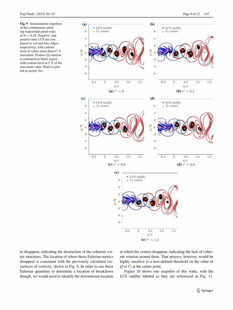
Figure 9 displays instantaneous snapshots of the wake from t∗ = 0.0 to t∗ = 1.2, where t∗ = t/T , and T is the period of panel pitching motion. The panel is continuously pitching, and t∗ = 0.0 is taken at the phase of motion where the panel is aligned with the flow, with the trailing edge moving in the positive y direction. From the trailing edge (x/c = 0.0) to approximately x/c = 1.5 downstream, the wake consists of a 2S vortex street. In the figure, it is clear that nLCS (red curves), pLCS (blue curves), and LCS sad-dles (cyan dots) provide a transverse boundary of the wake, and an alternating scroll pattern around the vortex cores. As each LCS saddle moves downstream, it approaches another saddle associated with a vortex shed in either the previous or subsequent half period. By approximately x/c = 1.0 downstream, the saddle pairs have nearly merged together entirely.

In addition, the Γ2 function and Q criterion have been calculated for this case. The function Γ2 is used here instead of Γ1 because of the large velocity of the whole vortex core, relative to the LEV velocity in the first example. In the first case, the LEV drifted from a relatively stable location. Here, the cores are continually moving downstream as part of the wake. As Γ1 is not Galilean invariant, its identifica-tion of the vortex center will be affected by the vortex core motion, whereas Γ2 will not be. The locations of the vortex cores as identified by Γ2 centers are shown as yellow dots, and the regions of positive Q criterion are the black round areas that give an indication of the vortex core regions. The contour setting for Q criterion is 5 % Qmax, so cho-sen to avoid small-scale noise associated with the experi-mental data. Farther than approximately one chord length downstream, both the Q regions and the Γ2 centers seem

Fig. 8 Spanwise vorticity (ωz) isosurfaces in the flow around a con-tinually oscillating trapezoidal panel. Panel is shown in black, posi-tive vorticity in white isosurfaces, negative vorticity in blue isosur-faces. Vorticity isosurface level is 14 % maximum and minimum ωz. Recreated from the data set of Green et al. (2011)

Exp Fluids (2015) 56:147

1 3

Page 9 of 12 147

to disappear, indicating the destruction of the coherent vor-tex structures. The location of where these Eulerian metrics disappear is consistent with the previously calculated iso-surfaces of vorticity, shown in Fig. 8. In order to use these Eulerian quantities to determine a location of breakdown though, we would need to identify the downstream location

at which the centers disappear, indicating the lack of coher-ent rotation around them. That process, however, would be highly sensitive to a user-defined threshold on the value of Q or Γ2 at the center point.

Figure 10 shows one snapshot of this wake, with the LCS saddles labeled as they are referenced in Fig. 11.

Fig. 9 Instantaneous snapshots of the continuously pitch-ing trapezoidal panel wake at St = 0.28. Negative- and positive-time LCS are con-toured as red and blue ridges, respectively, with contour level of values more than 67 % maximum. Positive Q criterion is contoured as black region with contour level at 5 % of the maximum value. Panel is plot-ted as purple line

-0.5 0 0.5 1.0 1.5

-2

0

2

4

6

-4

-6

x/c

y/A

LCS saddleΓ2 center

(a)

-0.5 0 0.5 1.0 1.5

-2

0

2

4

6

-4

-6

x/c

y/A

LCS saddleΓ2 center

(b)

-0.5 0 0.5 1.0 1.5

-2

0

2

4

6

-4

-6

x/c

y/A

LCS saddleΓ2 center

(c)

-0.5 0 0.5 1.0 1.5

-2

0

2

4

6

-4

-6

x/c

y/A

LCS saddleΓ2 center

(d)

-0.5 0 0.5 1.0 1.5

-2

0

2

4

6

-4

-6

x/c

y/A

LCS saddleΓ2 center

(e)

(a) t∗ = 0 (b) t∗ = 0.3

(c) t∗ = 0.6 (d) t∗ = 0.9

(e) t∗ = 1.2

Exp Fluids (2015) 56:147

1 3

147 Page 10 of 12

There are four markers labeled, two each that belong to boundaries of two subsequent structures along the cen-terline of the wake. They are labeled with either “H” to represent that they are on the higher half of the figure as presented, or “L” to represent that they are on the lower half of the figure as presented. Each of the distinct vortex cores has one H saddle and one L saddle, and as shown in Fig. 9, we expect the lower saddles to merge together, and the higher saddles to merge together. In particular, L1 and L2 are shown to approach merger in Fig. 9d at y/A ≈ −1 and x/c ≈ 1. H1 and H2 are shown to approach merger in Fig. 9d at y/A ≈ 1 and x/c ≈ 0.8.

In Fig. 11, the distance between the labeled H saddles and the distance between the labeled L saddles are pre-sented as a function of the downstream distance of each pair’s centroid. Both trace out a similar path as they move

downstream, with an apparent deceleration of the merg-ing occurring downstream of approximately 0.6 chord lengths. This is observed as a shallowing of the slope of the two curves. As shown in Fig. 9d, the lower half sad-dles approach each other at x/c ≈ 0.8, and the two red nLCS ridges that are associated with each of the two sad-dles become parallel to each other, but can never intersect. Therefore, the distance between the saddles will never go identically to zero. For this reason, we take the slope of these curves from trailing edge to x/c = 0.6, and find that both the upper half saddles and the lower half saddles have a projected merge location of x/c = 0.8 chord lengths downstream at St = 0.28.

In the previous work, the location of the vortex wake breakdown that accompanies the LCS saddle point merg-ers was shown to move upstream with increasing Strouhal number. By using the LCS analysis, a more direct and con-sistent analysis of the breakdown location is possible, and as in the current results, can identify and track these struc-tures with relatively less user interaction.

4 Summary

The vortex dynamics in two cases have been studied using a range of identification and tracking techniques: the flow around a 2D panel undergoing a transient pitch-up maneu-ver, and the wake downstream of a trapezoidal plate in purely pitching motion. The implementation of the analysis automatically detects dynamically significant points in the core and boundaries of vortex structures in a robust man-ner. In the case of the plate undergoing a pitch-up maneu-ver, tracking the LCS saddle points provides a direct identi-fication of leading-edge and trailing-edge vortex shedding: saddles associated with each vortex hold station in the flow before rapidly accelerating away at the time of vor-tex shedding. In contrast, Eulerian vortex core identifica-tion methods such as Γ1 and Q only show the core moving downstream at a relatively constant speed both while the attached vortex is still growing and while the vortex con-vects downstream after shedding. For the case of the trap-ezoidal panel pitching about its leading edge, the saddle tracking code is used to project a location of vortex break-down, following the work of Green et al. (2011). This early work qualitatively observed the breakdown as an interac-tion of LCS saddles from different vortices, which was not evident from a strictly Eulerian analysis, but did not pro-vide a quantitative technique to determine the downstream location of breakdown.

In the future, the methods developed here will be applied to other experimental and simulation data, especially in three dimensions, to verify and to continually improve the process. Once they are designed to track important

-0.5 0.0 0.5 1.0 1.5 2.0

-2.0

0.0

2.0

4.0

6.0

-4.0

-6.0

x/c

y/A

Fig. 10 Instantaneous snapshot of marked saddle points. Negative- and positive-time LCS are contoured as red and blue ridges, respec-tively, with contour level of values more than 67 % maximum. Posi-tive Q criterion is contoured as black region with contour level at 5 % of the maximum value. Panel is plotted as a purple line

0.2 0.4 0.6 0.8 1.00.0

0.1

0.2

0.3

0.4

Distance between saddle pair centroid and TE

L1 - L2

H1 - H2

Dista

ncebetwee

nsa

ddle

pair

Fig. 11 Decreasing distance between pairs of LCS saddles compared to downstream distance of the pair’s centroid. Two dotted lines indi-cate linear curve fits to the decreasing pair distances from upstream. Linear fit was performed for LCS saddle distance upstream of x/c = 0.6

Exp Fluids (2015) 56:147

1 3

Page 11 of 12 147

topological elements rigorously in three-dimensional space and time, these metrics have the potential to inform the design and implementation of feedback flow control. The saddles can be tracked back in time to their formation dur-ing a fluid-structure interaction, and their dynamics can be correlated with more easily sensed quantities, such as pres-sure or velocity on the body surface. With this information, strategies can be developed that utilize common control actuators in a more targeted manner to cause topological changes in the flow. In the current flow cases, this could be used to either promote or delay the phenomena of vortex shedding or vortex breakdown.

As a final note, use of the Lagrangian FTLE with experi-mental data requires both temporal and dimensional support in the data. While it is not uncommon to use a trajectory integration timestep during particle trajectory calculation that is smaller than the time between subsequent velocity data sets, the temporal resolution of the data must be suf-ficient so that interpolation techniques adequately recreate intermediate velocity fields when it is necessary. For inher-ently three-dimensional flows, a single plane of data, even if it contains all three velocity components, is not sufficient to generate an accurate Cauchy–Green deformation tensor and FTLE field. In particular, vortex structures that are par-allel to the data plane, such that the vortex-induced veloc-ity will be in and out of the plane, will not be captured. In those cases where it is known ahead of time that the struc-tures of interest are mainly perpendicular to the plane in which data are acquired, the FTLE calculation will capture the majority of the structures in the plane.

Acknowledgments Dr. Jeff Eldredge and his research group at UCLA are gratefully acknowledged for sharing the database of sim-ulation results for the current research. This work was supported by the Air Force Office of Scientific Research under AFOSR Award No. FA9550-14-1-0210 and by the Office of Naval Research under ONR Award No. N00014-14-1-0418.

References

Ahuja S, Rowley CW, Kevrekidis IG, Wei M, Colonius T, Tadmor G (2007) In: 45th AIAA aerospace sciences meeting and exhibit, AIAA Paper, vol 709

Anderson J, Streitlien K, Barrett D, Triantafyllou M (1998) Oscillat-ing foils of high propulsive efficiency. J Fluid Mech 360:41–72

Arora N, Gupta A, Sanghi S, Aono H, Shyy W (2014) Lift-drag and flow structures associated with the “clap and fling” motion. Phys Fluids (1994-present) 26(7):071906

Berson A, Michard M, Blanc-Benon P (2009) Vortex identification and tracking in unsteady flows. C R Mec 337(2):61–67

Borazjani I, Sotiropoulos F (2010) On the role of form and kinematics on the hydrodynamics of self-propelled body/caudal fin swim-ming. J Exp Biol 213(1):89–107

Brunton S, Rowley C (2009) Modeling the unsteady aerodynamic forces on small-scale wings. AIAA Pap 1127:2009

Buchholz JH, Smits AJ (2006) On the evolution of the wake struc-ture produced by a low-aspect-ratio pitching panel. J Fluid Mech 546:433–443

Buchholz JH, Smits AJ (2008) The wake structure and thrust perfor-mance of a rigid low-aspect-ratio pitching panel. J Fluid Mech 603:331–365

Cardwell BM, Mohseni K (2008) Vortex shedding over a two-dimensional airfoil: where the particles come from. AIAA J 46(3):545–547

Chakraborty P, Balachandar S, Adrian RJ (2005) On the relation-ships between local vortex identification schemes. J Fluid Mech 535:189–214

Chong M, Perry AE, Cantwell B (1990) A general classification of three-dimensional flow fields. Phys Fluids A Fluid Dyn (1989–1993) 2(5):765–777

Cucitore R, Quadrio M, Baron A (1999) On the effectiveness and lim-itations of local criteria for the identification of a vortex. Eur J Mech B Fluids 18(2):261–282

Dong H, Mittal R, Najjar F (2006) Wake topology and hydrodynamic performance of low-aspect-ratio flapping foils. J Fluid Mech 566:309–343

Eldredge JD (2007) Numerical simulation of the fluid dynamics of 2D rigid body motion with the vortex particle method. J Comput Phys 221:626–648

Eldredge JD, Chong K (2010) Fluid transport and coherent structures of translating and flapping wings. Interdiscip J Nonlinear Sci 20(1):017509

Ellington C (1984) The aerodynamics of hovering insect flight. IV. Aeorodynamic mechanisms. Philos Trans R Soc B Biol Sci 305(1122):79–113

Graftieaux L, Michard M, Grosjean N (2001) Combining PIV. POD and vortex identification algorithms for the study of unsteady turbulent swirling flows. Meas Sci Technol 12(9):1422

Green MA, Rowley CW, Haller G (2007) Detection of Lagrangian coherent structures in three-dimensional turbulence. J Fluid Mech 572:111–120

Green MA, Rowley CW, Smits AJ (2010) Using hyperbolic Lagran-gian coherent structures to investigate vortices in bioinspired fluid flows. Chaos 20(1):017510

Green MA, Rowley CW, Smits AJ (2011) The unsteady three-dimen-sional wake produced by a trapezoidal pitching panel. J Fluid Mech 685:117–145

Green MA, Smits AJ (2008) Effects of three-dimensionality on thrust production by a pitching panel. J Fluid Mech 615:211–220

Haller G (2001) Distinguished material surfaces and coherent struc-tures in 3D fluid flows. Phys D 149:248–277

Haller G (2002) Lagrangian coherent structures from approximate velocity data. Phys Fluids 14(6):1851–1861

Haller G (2005) An objective definition of a vortex. J Fluid Mech 525:1–26

Hunt JCR, Wray A, Moin P (1988) Eddies, stream, and convergence zones in turbulent flows. Center for turbulence research report CTR-S88, pp 193–208

Jeong J, Hussain F (1995) On the identification of a vortex. J Fluid Mech 285:69–94

Kaplan S, Altman A, Ol M (2007) Wake vorticity measurements for low aspect ratio wings at low Reynolds number. J Aircr 44(1):241–251

Koochesfahani MM (1989) Vortical patterns in the wake of an oscil-lating airfoil. AIAA J 27(9):1200–1205

Lekien F, Shadden SC, Marsden JE (2007) Lagrangian coherent struc-tures in n-dimensional systems. J Math Phys 48(6):065404

Lipinski D, Cardwell B, Mohseni K (2008) A Lagrangian analysis of a two-dimensional airfoil with vortex shedding. J Phys A Math Theor 41(34):344011

Exp Fluids (2015) 56:147

1 3

147 Page 12 of 12

Magill J, Bachmann M, Rixon G, McManus K (2003) Dynamic stall control using a model-based observer. J Aircr 40(2):355–362

Mathur M, Haller G, Peacock T, Ruppert-Felsot JE, Swinney HL (2007) Uncovering the Lagrangian skeleton of turbulence. Phys Rev Lett 98(14):144502

O’Farrell C, Dabiri JO (2014) Pinch-off of non-axisymmetric vortex rings. J Fluid Mech 740:61–96

Ol MV, McAuliffe BR, Hanff ES, Scholz U, Kähler C (2005) Com-parison of laminar separation bubble measurements on a low Reynolds number airfoil in three facilities. AIAA paper 2005-5149

Peng J, Dabiri JO (2008) The ‘upstream wake’ of swimming and fly-ing animals and its correlation with propulsive efficiency. J Exp Biol 211(16):2669–2677

Peng J, Dabiri J (2009) Transport of inertial particles by Lagrangian coherent structures: application to predator–prey interaction in jellyfish feeding. J Fluid Mech 623:75–84

Pitt Ford C, Babinsky H (2013) Lift and the leading-edge vortex. J Fluid Mech 720:280–313

Ringuette MJ, Milano M, Gharib M (2007) Role of the tip vortex in the force generation of low-aspect-ratio normal flat plates. J Fluid Mech 581:453–468

Sane SP (2003) The aerodynamics of insect flight. J Exp Biol 206(23):4191–4208

Shadden SC, Dabiri JO, Marsden JE (2006) Lagrangian analysis of fluid transport in empirical vortex ring flows. Phys Fluids (1994-present) 18(4):047105

Shadden SC, Lekien F, Paduan JD, Chavez FP, Marsden JE (2009) The correlation between surface drifters and coherent structures based on high-frequency radar data in Monterey Bay. Deep Sea Res Part II Top Stud Oceanogr 56(3):161–172

Smith AC, Baillieul J (2003) In: Decision and control. Proceed-ings. 42nd IEEE conference on, vol 3 (IEEE, 2003), vol 3, pp 2407–2412

Triantafyllou M, Triantafyllou G, Yue D (2000) Hydrodynamics of fishlike swimming. Annu Rev Fluid Mech 32(1):33–53

Videler J, Stamhuis E, Povel G (2004) Leading-edge vortex lifts swifts. Science 306(5703):1960–1962

Voth GA, Haller G, Gollub JP (2002) Experimental measurements of stretching fields in fluid mixing. Phys Rev Lett 88(25):254501

Wang Z (2000) Vortex shedding and frequency selection in flapping flight. J Fluid Mech 410:323–341

Wang C, Eldredge JD (2012) Low-order phenomenological modeling of leading-edge vortex formation. Theor Comput Fluid Dyn 27:577–598

Weldon M, Peacock T, Jacobs G, Helu M, Haller G (2008) Experi-mental and numerical investigation of the kinematic theory of unsteady separation. J Fluid Mech 611:1–11

Yang Y, Pullin D (2011) Geometric study of Lagrangian and Eulerian structures in turbulent channel flow. J Fluid Mech 674:67–92

Young J, Lai JC (2007) Vortex lock-in phenomenon in the wake of a plunging airfoil. AIAA J 45(2):485–490

Zbikowski R (2002) On aerodynamic modelling of an insect-like flap-ping wing in hover for micro air vehicles. Philos Trans R Soc Lond A Math Phys Eng Sci 360(1791):273–290

Zhou J, Adrian RJ, Balachandar S, Kendall T (1999) Mechanisms for generating coherent packets of hairpin vortices in channel flow. J Fluid Mech 387:353–396