detecting possibly saturated positions in 18s and 28s sequences and their influence on phylogenetic...

Molecular Phylogenetics and Evolution 48 (2008) 628–645

Contents lists available at ScienceDirect

Molecular Phylogenetics and Evolution

journal homepage: www.elsevier .com/locate /ympev

Detecting possibly saturated positions in 18S and 28S sequences and theirinfluence on phylogenetic reconstruction of Annelida (Lophotrochozoa)

Torsten H. Struck a,b,*, Maximilian P. Nesnidal b, Günter Purschke b, Kenneth M. Halanych a

a Auburn University, 101 Rouse Building, Auburn, AL 36849, USAb Universität Osnabrück, FB05 Biologie/Chemie, AG Zoologie, Barbarastrabe 11, D-49076 Osnabrück, Germany

a r t i c l e i n f o

Article history:Received 11 November 2007Revised 25 April 2008Accepted 13 May 2008Available online 20 May 2008

Keywords:C factorO/E ratioAnnelidaSaturationrRNAPhylogenyIss

1055-7903/$ - see front matter � 2008 Elsevier Inc. Adoi:10.1016/j.ympev.2008.05.015

* Corresponding author. Address: Universität OsnaAG Zoologie, Barbarastrabe 11, D-49076 Osnabrück,2587.

E-mail addresses: [email protected] (M.P. Nesnidal), [email protected]@auburn.edu (K.M. Halanych).

a b s t r a c t

Phylogenetic reconstructions may be hampered by multiple substitutions in nucleotide positions obliter-ating signal, a phenomenon called saturation. Traditionally, plotting ti/tv ratios against genetic distanceshas been used to reveal saturation by assessing when ti/tv stabilizes at 1. However, interpretation ofresults and assessment of comparability between different data sets or partitions are rather subjective.Herein, we present the new C factor, which quantifies convergence of ti/tv ratios, thus allowing compa-rability. Furthermore, we introduce a comparative value for homoplasy, the O/E ratio, based on alterationsof tree length. Simulation studies and an empirical example, based on annelid rRNA-gene sequences,show that the C factor correlates with noise, tree length and genetic distance and therefore is a proxyfor saturation. The O/E ratio correlates with the C factor, which does not provide an intrinsic thresholdof exclusion, and thus both together can objectively guide decisions to exclude saturated nucleotide posi-tions. However, analyses also showed that, for reconstructing annelid phylogeny using Maximum Likeli-hood, an increase in numbers of positions improves tree reconstruction more than does the exclusion ofsaturated positions.

� 2008 Elsevier Inc. All rights reserved.

1. Introduction

Reliable reconstruction of phylogenies using molecular data isaffected by several factors such as long branches, heterogeneityof base frequencies, and rate heterogeneity among positions (e.g.,Kuhner and Felsenstein, 1994; Lake, 1994; Lockhart et al., 1994;Xia et al., 2003). All of these factors can result in homoplasy, whichcan decrease phylogenetic signal and hamper reconstruction ef-forts. An indicator of homoplasy in molecular data sets can be sat-uration of transition events relative to other mutations (e.g.,Halanych and Robinson, 1999; Jördens et al., 2004; Lopez et al.,1999; Nickrent et al., 2000; Philippe and Forterre, 1999; Simonet al., 1994; Struck et al., 2002a; Swofford et al., 1996). Saturationis invoked when no further increase in transitions can be observeddespite increasing genetic distance, indicating that multiple substi-tutions at nucleotide positions have occurred. Therefore, when adata set is saturated, phylogenetic reconstruction may be misledby homoplasious signal (e.g., Milinkovitch et al., 1996; Simonet al., 1994). Saturation is especially problematic for taxa that radi-

ll rights reserved.

brück, FB05 Biologie/Chemie,Germany. Fax: +49 541 969

.de (T.H. Struck), [email protected] (G. Purschke),

ated rapidly long ago. For example, the radiation of annelid wormswithin Lophotrochozoa apparently was fast and resulted inbranching patterns with short internodes in the basal part of theannelid tree and with branch lengths rapidly increasing towardsthe tips. Such branching patterns accumulate only a few informa-tive substitutions along the internal and more basal branches,but numerous homoplasious substitutions on terminal branches(Struck et al., 2002a). For example, in Struck et al.’s (2007) analysesof three nuclear genes, the ratio of terminal branch length to inter-nal branch length is 4.2/1 even excluding the extremely longbranch leading to the highly divergent taxon, Ophryotrocha labron-ica. Thus, phylogenetic information is likely to be eroded due tomultiple substitutions, or homoplasy, along the terminal branches.To avoid these problems, several authors have used conservativegenes such as elongation factor 1a, 18S and/or 28S rDNA (e.g., Re-gier and Shultz, 1997; Struck et al., 2002a, 2007; Xia et al., 2003).However, even in these genes certain regions may be saturatedand therefore mislead reconstruction. In contrast, excluding prob-lematic regions may leave too little phylogenetic information to re-solve the deep branches (Xia et al., 2003).

Traditionally, saturation is shown by plotting either numbers ofsubstitutions or the transition-to-transversion (ti/tv) ratios of allpairwise comparisons of taxa in an alignment against the geneticdistances (p) between these pairs (e.g., Halanych and Robinson,1999; Jördens et al., 2004; Struck et al., 2002a). In the latter case, con-vergence upon a ti/tv value of 1 is expected with the approach of

mailto:[email protected]

mailto:nesnidal@ gmail.com

mailto:nesnidal@ gmail.com



http://www.sciencedirect.com/science/journal/10557903

http://www.elsevier.com/locate/ympev

T.H. Struck et al. / Molecular Phylogenetics and Evolution 48 (2008) 628–645 629

saturation at higher genetic distances. Generally, plotting ti/tv ratios ismore useful because it integrates properties of two substitution types.However, identifying saturation is subjective when using such plots:Whether or not to include a gene or certain subsets of a gene (i.e., posi-tions that exhibit only slight saturation or strong saturation) may beobvious, but whether to incorporate or eliminate positions with inter-mediate stages of saturation is not straightforward and lacks objectiv-ity (Struck et al., 2007). Furthermore, with an increasing number oftaxa and genes or subsets of genes, the representation of the plotswithin one graph becomes increasingly problematic (Struck et al.,2007). A comprehensive method of display would promote compari-son of plots and aid objective decision-making.

Due to convergence upon a value, the distribution of the ti/tvvalues of the pairwise comparisons covers an increasingly smallerrange of values as genetic distance increases, and thus the standarddeviation of this distribution [r(ti/tv)] decreases with increasingsaturation. On the other hand, the distribution of the genetic dis-tances p of these pairwise comparisons becomes more spread outand thus the standard deviation of this distribution [r(p)] isincreasing. By extrapolating from this behavior of convergence,we developed a convergence factor (C factor), which is based onthe ratio of the standard deviation of the ti/tv distribution to thestandard deviation of the p distribution:

C ¼rð ti

tvÞrðpÞ ð1Þ

The C factor is determined before, and independently of, the treereconstruction and thus is an a priori approach.

Next, using the parsimony criterion we developed another factorto assess the degree of homoplasy. This one being based on alterationof tree lengths is an a posteriori approach. Given a data set withouthomoplasy, removal of any subset of the data reduces tree lengthby an amount directly proportional to the reduction in the minimumnumber of substitutions necessary to explain the data set. Becauseeach substitution is one step of the tree length, the relative changeis the same for both, tree length and number of substitutions, andthus their ratio is 1. Given a starting tree length of l, alteration in treelength can be expressed as the observed change O and the reductionin minimum necessary substitutions s as the expected change, E,assuming no homoplasy in the data set:

O ¼ lrlc

ð2Þ

and

E ¼ sr

scð3Þ

For both l and s, the subscript c indicates the value for thecomplete, initial data set, and subscript r indicates the value forthe reduced data set. Their ratio can be given as O/E. An easyway to calculate this ratio is to estimate the ratio of the consistencyindices CIc/CIr:

OE¼ lr=lc

sr=sc¼ lr

sr� sc

lc¼ 1

CIr� CIc ¼

CIc

CIrð4Þ

In empirical data sets, homoplasious substitutions contributemore to the tree length than do the synapomorphic ones, becausethey require at least two steps instead of one. Therefore, if the re-moved subset is less homoplasious than the complete data set, theO/E ratio is >1, because fewer steps were excluded from the dataset than expected from the reduction in substitutions. In otherwords, lr is larger than expected. On the other hand, if the removedsubset is more homoplasious than the complete set, then O/E is <1,because lr is smaller than expected. An O/E ratio of 1 indicates thatthe removed part has the same degree of homoplasy as the completedata set.

Herein, we tested both our new factors—C and O/E—using sim-ulation studies as well as a real data set derived from 18S and 28Ssequences of Annelida.

1.1. On the Annelida

As mentioned, Annelida are part of the rapid radiation of lopho-trochozoan animals that occurred in or before the early Cambrian;besides annelids, Lophotrochozoa also includes mollusks, platy-helminths, brachiopods, nemerteans, rotifers and several othertaxa (Halanych, 2004; McHugh, 2000, 2005). Annelida comprisesan ecologically important animal phylum with over 16,500 de-scribed species, and its members include the dominant macrofa-una of the deep sea. Traditionally two major groups have beendistinguished: Clitellata (earthworms, leeches) and Polychaeta(e.g., Fauchald and Rouse, 1997; Westheide, 1997; Westheide etal., 1999). Monophyly of Clitellata is well-supported by both mor-phological and molecular data (e.g., Erséus, 2005; Erséus and Kal-lersjo, 2004; Purschke, 2002; Struck and Purschke, 2005).However, Polychaeta has proven more problematic. Cladistic anal-yses based on morphological data seem to support a monophyleticPolychaeta (Rouse and Fauchald, 1997), but recent molecular phy-logenetic studies reject monophyly of polychaetes, as well as oftheir traditional subgroups (e.g., Rousset et al., 2007; Struck etal., 2007). Additionally, Siboglinidae (a.k.a. Pogonophora and Ves-timentifera; beard worms) and Echiura (spoon worms; as sisterto Capitellidae) have also to be included in Annelida (e.g., Bartolo-maeus, 1995; Bleidorn et al., 2003b; Hessling, 2002; McHugh,1997; Struck et al., 2007). Furthermore, Sipuncula (peanut worms)are discussed as either an annelid subtaxon or their sister group(e.g., Bleidorn et al., 2006; Struck et al., 2007; Tzetlin and Purschke,2006). Unfortunately, well-supported more-inclusive groupings ofthe approximately 80 polychaete families are largely lacking.

Although some recent studies used up to five genes, molecularanalyses addressing annelid phylogeny are mainly based on the18S and 28S genes (Colgan et al., 2006; Rousset et al., 2007; Strucket al., 2007). Different molecular analyses of annelid phylogenyhave treated the problem of saturated positions in different ways.Some did not exclude any positions at all (e.g., Rousset et al., 2007),others excluded ambiguously aligned ones (e.g., Colgan et al.,2006), and others also excluded saturated ones (e.g., Jördens etal., 2004; Struck et al., 2007). Furthermore, although complete18S was always used, different parts of the 28S have been in-cluded: the nearly complete sequence of 3.3 kilobases (kb) (Strucket al., 2005, 2007), the so-called D1 (0.3 kb) and/or D9/10 (0.6 kb)fragments (Brown et al., 1999; Colgan et al., 2006; Rousset et al.,2007) or a fragment comprising the region between these two frag-ments of about 2.2 kb (Jördens et al., 2004).

Herein we evaluated our saturation factors, C and O/E, usingsimulation studies as well as a data set of 18S and 28S sequencesfrom 98 annelid and 9 lophotrochozoan outgroup taxa. Further-more, we determined how likely three different fragments of 28Sare to saturate, compared to nearly complete sequences of 28Sand 18S. Additionally, we propose an improvement of the slidingwindow analysis for rRNA and similar genes to group positionswith similar genetic variation within one partition.

2. Material and methods

2.1. Simulated data

To model simulation studies on an empirical tree, we selected18S and 28S sequences of 9 polychaete and 1 outgroup from Strucket al. (2007). This taxonomic subsample was evenly distributed ontheir tree and represented the variety of branch lengths they recov-

630 T.H. Struck et al. / Molecular Phylogenetics and Evolution 48 (2008) 628–645

ered. Chosen operational taxonomic units (OTUs) were Glycera,Sthenalanella, Drilonereis, Ninoe, Pectinaria, Ophelina, Notomastus,Polydora, Chaetopterus and Crassostrea (mollusk outgroup), andwith these sequences we reconstructed the ML tree. The appropri-ate model of sequence evolution, Tamura & Nei + I + C, was deter-mined based on the AIC criterion in Modeltest V 3.7 (Posada andCrandall, 1998, 2001). The estimated model parameters were: basefrequencies: A = 0.2514, C = 0.2275, G = 0.3017, T = 0.2194; substi-tution rates: A M C, A M T, C M G, G M T = 1.0000, A M G = 1.8754,C M T = 4.7929; a = 0.6216, number of categories = 4; proportionof invariant sites = 0.4575. ML tree reconstruction based on thesemodel parameters employed PAUP*4.0b (Swofford, 2002) with 10random taxon additions and tree bisection-reconnection (TBR)branch swapping.

Simulated data sets based on this ML tree (Fig. 1) and on thecorresponding model parameters were generated using Mesquitev1.05 (Maddison and Maddison, 2004). By definition the initialdata set had no or only a low degree of homoplasy or saturation,so we introduced these features in two ways. In the first strategy,we altered the evolutionary rate along the whole tree using differ-ent scale factors (0.1, 0.5, 1, 2, 10). This means that each branch ofthe tree was varied from one tenth to ten times the length of thebranch shown in Fig. 1. Thus, the evolutionary rates were madeto vary by a factor of 100 over the simulations. Note that, the sim-ulations using a scale factor of 0.1 had the slowest evolutionaryrates and the lowest degree of homoplasy. Subsequently, data setsgenerated for the second strategy were based on a scale factor of0.1 to ensure that both strategies had similar, low, initial degreesof homoplasy. For the second strategy, we directly introduced ran-dom data (i.e., noise) using the option ‘‘random fill” in Mesquitev1.05 (Maddison and Maddison, 2004). In the different trials, 0%,5%, 10%, 25% or 50% of the positions were randomized. For bothstrategies and for each individual option (i.e., 0%, 5%, 10%, 25%and 50% noise or scale factors of 0.1, 0.5, 1, 2 and 10), we simulated50 individual data sets with 300 nucleotide positions resulting intotal 10 times 50 (=500) data sets.

0.1

Taxon 4

Taxon 10

Taxon 5

Taxon 6

Taxon 7

Taxon 3

Taxon 9

Taxon 8

Taxon 1

Taxon 2

Fig. 1. Tree used in simulation study. Phylogram of ML analysis of 9 annelid and 1outgroup OTUs (Glycera, Sthenalanella, Drilonereis, Ninoe, Pectinaria, Ophelina,Notomastus, Polydora, Chaetopterus and Crassostrea). �lnL = 12625.63033. OTUnames have been concealed, because the tree was generated for simulationpurposes only.

For each individual data set, we were able to determine the Cfactor directly. However, the O/E ratio is a relative factor comparinga data set reduced by a certain partition against the complete dataset. Therefore, to calculate the O/E ratio we had to concatenateindividual data sets generated for each of the two strategies andfive options, respectively. Because we were interested in the corre-lation of the O/E ratio with both saturation and the C factor, weconcatenated for each strategy five individual data sets, one fromeach of the five options. For example, for the first strategy usingscale factors we concatenated five individual data sets, one fromeach of the 50 data sets generated by a scale factor of 0.1, 0.5, 1,2 or 10, respectively. For the second strategy, such a concatenateddata set consisted of five individual data sets, one from each of the50 data sets generated using 0%, 5%, 10%, 25% or 50% noise level,respectively. Thus, we got 2 times 50 concatenated data sets gen-erated from the 10 times 50 individual data sets. This concatena-tion procedure allowed assessing the correlation of the O/E ratiowith both saturation (i.e., 0%, 5%, 10%, 25% and 50% noise, or scalefactors of 0.1, 0.5, 1, 2 and 10) and the determined C factor of theindividual data.

Finally, we also investigated if an increased number of positionsresults in an increased recovery of the true tree. Therefore, we sim-ulated 50 data sets with 100, 300, 500, 1000, 2000 or 5000 posi-tions, respectively, using a scale factor of 1. Herein, we used ascale factor of 1 in contrast to 0.1 as the initial degree of homoplasyto be able to compare these results with the results we got fromthe empirical data of Annelida. We determined the C factor as wellas the MP and ML tree for each data set using 10 random taxonadditions and TBR branch swapping in PAUP*4.0b (Swofford,2002).

2.2. Empirical data

The empirical data set comprised 107 OTUs of Annelida andoutgroups including new sequence data of 18S and 28S determinedfor 11 and 16 polychaete OTUs, respectively.

2.3. Collection of data and sequence alignment

Table 1 lists the taxa, gene sequences and GenBank accessionnumbers used in this study. Upon collection, tissue samples orwhole individuals were preserved in >70% non-denatured EtOHor frozen at �80 �C. Genomic DNA was extracted using the DNeasyTissue Kit (Qiagen). Amplification and sequencing of the nuclear18S and 28S rDNA were carried out using protocols described byStruck et al. (2006). All products were verified on a 1% agarosegel and purified with the QIAquick PCR Purification Kit (Qiagen).As necessary, PCR products were size-selected on agarose gelsand/or cloned using the pGEM�-T Easy Vector System (Promega).A CEQTM 8000 Genetic Analysis System (Beckman Coulter) usingCEQ dye terminator chemistry was used for bidirectional sequenc-ing of all products.

Because Annelida are part of the poorly resolved lophotrocho-zoan clade (Halanych, 2004), their sister group is not known yet,so several other lophotrochozoan taxa were employed as outgrouptaxa (see Table 1). Sequences were aligned with CLUSTAL W usingdefault settings (Thompson et al., 1994) and subsequently cor-rected by hand in GeneDoc (Nicholas and Nicholas, 1997). Ambig-uous positions were determined using GBlocks (Castresana, 2000)with default settings except the allowed gap positions, which wereset to ‘‘with half”. Positions possessing a gap in less than 50% of thesequences are not excluded a priori, but can be selected in the finalalignment if they are within an appropriate block. After the deter-mination of classes of identity, all ambiguous positions were ex-cluded from all subsequent analyses. The alignment (Accession#S2045) is available at TREEBASE (http://www.treebase.org).

http://www.treebase.org

Table 1List of the taxa used in the analyses with 18S and 28S sequence accession numbers

Taxon Species 18S 28S

AnnelidaArenicolidae Arenicola brasiliensis (Nonato, 1958) DQ790076

Abarenicola affinis (Ashworth, 1903) DQ790025

Capitellidae Heteromastus filiformis (Claparede, 1864) DQ790081 DQ790038Notomastus tenuis Moore, 1909 DQ790084 DQ790044

Maldanidae Clymenella torquata (Leidy, 1855) DQ790030Clymenura clypeata (Saint-Joseph, 1894) AF448152Axiothella rubrocincta (Johnson, 1901) DQ790078 DQ790027

Opheliidae Armandia brevis (Moore, 1906)a EU418854 EU418862Ophelia rathkei McIntosh, 1908 AF448157 AY366513Ophelina acuminata Oersted, 1843 DQ790085 DQ790045

Orbiniidae Orbinia swani Pettibone, 1957 DQ790087 DQ790048Scoloplos fragilis (Verrill, 1873)b AY532360 EU418863

Paranoidae Aricidea sp.c EU418855 DQ790052

Scalibregmatidae Scalibregma inflatum Rathke, 1843 DQ790093 DQ790060Travisia brevis Moore, 1923 DQ790069Travisia forbesii Johnston, 1840 AF508127

Aphroditidae Aphrodita sp. AY894295 DQ790024

Polynoidae Gattyana ciliata Moore, 1902 AY894297 DQ790035Lepidonotus sublevis Verrill, 1873 AY894301 DQ790039

Sigalionidae Sigalion spinosus (Hartman, 1939) AY894304 DQ790062Sthenelanella uniformis Moore, 1910 AY894306 DQ790064

Hesionidae Ophiodromus pugettensis (Johnson, 1901) DQ790086 DQ790046

Nereididae Nereis succinea (Frey and Leuchart, 1847) AY210447 AY210464Nereis vexillosa Grube, 1851 DQ790083 DQ790043

Pilargidae Ancistrosyllis groenlandica McIntosh, 1879 DQ790075 DQ790023

Syllidae Exogone naidina Oersted, 1845 AF474290Exogone verugera (Claparede, 1868) DQ790033Proceraea cornuta (Agassiz, 1862) AF474312 AF212165Typosyllis anoculata (Hartmann-Schröder, 1962) DQ790098 DQ790071

Glyceridae Glycera dibranchiata Ehlers, 1868 AY995208 AY995207Glycera americana Leidy, 1855d EU418856 EU418864

Goniadidae Goniada brunnea Treadwell, 1906 DQ790080 DQ790037Glycinde armigera Moore, 1911 DQ790079 DQ790036

Nephtyidae Nephtys longosetosa (Oersted, 1842) DQ790082 DQ790042Nephtys incisa Malmgren, 1865e EU418857 EU418865Aglaophamus circinata (Verrill, 1874) DQ790072 DQ790020

Paralacydoniidae Paralacydonia paradoxa Fauvel, 1913 DQ790088 DQ790050

Phyllodocidae Phyllodoce groenlandica (Oersted, 1843) DQ790092 DQ790055

Alciopidae Alciopina sp. DQ790073 DQ790021Torrea sp. DQ790096 DQ790068

Tomopteridae Tomopteris sp. DQ790095 DQ790067

Amphinomidae Paramphinome jeffreysii (Mcintosh, 1868) AY838856 AY838865Eurythoë complanata (Pallas, 1766) AY364851 AY364849

Dorvilleidae Protodorvillea kefersteini (McIntosh, 1869) AF412799 AY732230Parougia eliasoni (Oug, 1978) AF412798 DQ790053

Eunicidae Marphysa sanguinea (Montagu, 1815) AY525621 AY838861Eunice sp. AF412791 AY732229

Lumbrineridae Lumbrineris latreilli Audouin & Milne-Edwards, 1834 AY525623 AY366512Lumbrineris inflata (Moore, 1911) AY525622 AY364864Ninoe nigripes Pettibone, 1982 AY838852 AY838862

Oenonidae Arabella semimaculata (Moore, 1911) AY838844 AY838857Drilonereis longa Webster, 1879 AY838847 AY838860Oenone fulgida Pettibone, 1982 AY838853 AY838863

Onuphidae Diopatra aciculata Knox and Cameron, 1971 AY838845 AY838858Hyalinoecia tubicola O.F. Müller, 1776 AF412794 AY732228

Oweniidae Owenia fusiformis delle Chiaje, 1841 AF448160 DQ790049

Sabellaridae Sabellaria cementarium Moore, 1906 AY732223 AY732226

Sabellidae Schizobranchia insignis Bush, 1905 AY732222 AY732225Serpulidae Serpula vermicularis Linnaeus, 1767 AY732224 AY732227

Siboglinidae Riftia pachyptila Jones, 1981 AF168739 Z21534Siboglinum fiordicum Webb, 1963 X79876 DQ790061

Cirratulidae Cirratulus spectabilis (Kinberg, 1866) AY708536 DQ790029

(continued on next page)


Table 1 (continued)

Taxon Species 18S 28S

Ctenodrilidae Ctenodrilus serratus (Schmidt, 1857) AY364850 AY364864

Fauveliopsidae Fauveliopsis scabra Hartman & Fauchald, 1971 AY708537 DQ790034

Flabelligeridae Diplocirrus glaucus (Malmgren, 1867) AY708534 DQ790031Pherusa plumosa (Müller, 1776) AY708528 DQ790056

Poeobiidae Poeobius meseres Heath, 1930 AY708526 DQ790058

Sternaspidae Sternaspis scutata (Ranzani, 1817) AY532329 DQ790063

Ampharetidae Auchenoplax crinita Ehlers, 1887 DQ790077 DQ790026

Pectinariidae Pectinaria gouldi (Verrill, 1873) DQ790091 DQ790054

Terebellidae Amphitrite ornata (Leidy, 1855) DQ790074 DQ790022Pista cristata (O. F. Mueller, 1776) AY611461 DQ790057Polycirrus sp.f EU418858 EU418866

Trichobranchidae Terebellides stroemi Sars, 1835 DQ790094 DQ790066

Chaetopteridae Chaetopterus variopedatus (Renier, 1804) U67324 AY145399

Spionidae Polydora ciliata (Johnston, 1838) U50971Polydora sp. DQ790059Prionospio dubia Maciolek, 1985g EU418859 EU418867Scolecolepis viridis Verrill, 1873h EU418860 EU418868

Trochochaetidae Trochochaeta sp. DQ790097 DQ790070

Poecilochaetidae Poecilochaetus serpens Allen, 1904i AY569652 EU418869

Apistobranchidae Apistobranchus typicus (Webster & Benedict, 1887)i AF448150 EU418870

Clitellata Lumbricus terrestris Linnaeus, 1758 AJ272183Lumbricus sp. DQ790041Lumbriculus variegatus (Mueller, 1774) AY040693Lumbriculus sp. DQ790040Eisenia foetida Savigny, 1826 AB076887Eisenia sp. DQ790032Stylaria sp. U95946 DQ790065Erpobdella octoculata (Linnaeus, 1758) AF099949 AY364865Hirudo medicinalis Linnaeus, 1758 Z83752 AY364866

Aeolosomatidae Aeolosoma sp. Z83748 DQ790019

Parergodrilidae Parergodrilus heideri Reisinger, 1925 AJ310504 AY366514Stygocapitella subterranea Knöllner, 1934 AF412810 AY366516Hrabeiella periglandulata Pizl & Chalupsky, 1984 AJ310501 AY364867

Dinophilidae Trilobodrilus axi Westheide, 1967 AF412806 AY732231Trilobodrilus heideri Remane, 1925 AF412807 AY894292

Nerillidae Leptonerilla prospera (Sterrer & Iliffe, 1982)j AY834758 EU418871

Polygordiidae Polygordius appendicularis (Fraipont, 1887)k AY525629 EU418872

Protodrilidae Protodrilus ciliatus Jägersten, 1952k AY525631 EU418873Protodrilus purpureus (Schneider, 1868)k AY527057 EU418874

Protodriloidae Protodriloides chaetifer (Remane, 1926)l AY527058 EU418875Protodriloides symbioticus (Giard, 1904)l AF508125 EU418876

Saccocirridae Saccocirrus sp.m EU418861 EU418877

Echiura Arhynchite pugettensis Fisher, 1949 AY210441 AY210455Urechis caupo Fisher & MacGinitie, 1928 AF119076 AF519268

Sipuncula Phascolopsis gouldi (Pourtalès, 1851) AF342796 AF342795

OutgroupsBivalvia Crassostrea virginica (Gmelin, 1791) AB064942 AY145400

Solemya velum Say, 1822 AF120524 AY145421Yoldia limaluta (Say, 1831) AF120528 AY145424

Gastropoda Ilyanassa obsoleta (Say, 1822) AY145379 AY145411

Polyplacophora Chaetopleura apiculata (Say, 1834) AY145370 AY145398

Brachiopoda Terebratalia transversa (Sowerby, 1846) AF025945 AF342802Glottidia pyramidata (Stimpson, 1860) U12647 AY210459

Nemertea Cerebratulus lacteus (Leidy, 1851) AY145368 AY145396


Table 1 (continued)

Sequences that were newly obtained for the present study are indicated in boldface.a Locality: 48�32.971’N/122�55.378’W, Lopez Island, WA, USA; Specimen voucher: USNM 1112639.b Locality: Little Buttermilk Bay, MA, USA; Specimen voucher: USNM 1112638.c Locality: 39�58.397’N/70�40.281’W, Southern New England, MA, USA; Specimen voucher: USNM 1112641.d Locality: 41�43.250’N/70�20.150’W, Land grant area 1, Barnstable Harbor, MA, USA; Specimen voucher: USNM 1112637.e Locality: 40�53.019’N/70�25.003’W, Southern New England, MA, USA; Specimen voucher: USNM 1112640.f Locality: 40�35.596’N/71�31.911’W, Southern New England, MA, USA; Specimen voucher: USNM 1112642.g Locality: 39�56.172’N/69�34.573’W, Southern New England, MA, USA; completely used.h Locality: 41�41.484’N/70�37.612’W, Barlow’s Landing, MA, USA; Specimen voucher: USNM 1112636.i kindly provided by C. Bleidorn (University of Potsdam) (Bleidorn et al., 2003a, 2005).j kindly provided by K. Worsaae (University of Kopenhagen) (Worsaae et al., 2005).k Locality: North Sea island Helgoland, Germany; completely used.l Locality: List, North Sea island Sylt, Germany; completely used.

m Locality: Giglio, Italy; completely used.


2.4. Determination of classes of identity

Saturation can be investigated for complete genes or for subsetsof characters (sites) within genes that share a certain property.Such groups are called classes of identity (Vogt, 2002). Differentsites within genes can show tremendous differences in substitu-tion rates with some characters seemingly static and others expe-riencing numerous substitutions (Yang, 1993, 1996). Therefore,various regions of a gene can be treated differently. For structuralgenes, like the small and large subunit ribosomal RNA genes, vari-able and conserved parts have been characterized (e.g., Hassounaet al., 1984; Mallatt et al., 2001; Zardoya and Meyer, 2001). The for-mer are the so-called divergent domains (D1-12) in 28S and thevariable regions (V1-9) in 18S. Plots on tertiary structure predic-tions reveal that the degree of variability depends on the distancefrom the ribosome center and is continuously changing (Wuyts etal., 2001). Therefore, we wanted to distinguish between more thanjust these two basic classes of identity (conserved vs. variable) toget more rate categories (classes of identity).

An approach using information contained in the data set seemsto be promising for discriminating more classes of identity. Variousauthors have performed sliding window analyses examining thedegree of variation in nucleotide positions (e.g., Jördens et al.,2004; Pesole et al., 1992; Struck et al., 2002a; Sturmbauer andMeyer, 1992). Variation is examined within a window of nine char-acters (Fig. 2). Assuming a priori for each substitution that it is not

... 61 62 63 64 65 66 67

67

11.1%

...

...

61 62 63 64 65 66

61 62 63 64 65 66

67

11.1%

move on 6 chara

Sliding window

Assigned degree of variation

... 1 0 1 0 0 0 0Minimally necessary substitutions

... C G T A A G

... A C G T A A G

... A C G T A A G

... A C T A A GAlignment

T

C

Fig. 2. Hypothetical scheme illustrating the traditional sliding window analysis. The minbelow the alignment. Character positions in the alignment are shown as 61–77, and thevariation.

homoplasious (Hennig’s auxiliary principle), the degree of varia-tion is expressed as a percentage of the 27 maximally possible sub-stitutions in a window of nine characters. For example, if such awindow has six constant characters across some number of taxaand three characters that possess two nucleotide states acrossthe same taxa, the window would be said to exhibit at least threesubstitutions assuming Hennig’s auxiliary principle. The degree ofvariation of this window would be 11.1% (3 characters with mini-mally one substitution/27 maximally possible substitutions). Thewindow then slides over 6 characters (resulting in an overlap ofthree characters with the previous window) and the degree of var-iation (11.1% here) is assigned to the six characters left behind inthe previous window. The degree of variation is determined aneweach time the window slides down the alignment. The degreeranges from 0% to 100%. Classes of identity are assigned to 10%increments of genetic variation. To some degree, this procedure re-flects a discrete C distribution (Yang, 1993, 1996).

This sliding-window procedure has a problem, however. Inclu-sion of an insertion not in frame with the number of characters thewindow slides down each step (i.e., six characters herein) has ashifting effect on all windows downstream from this insertion,even if the sequence with the indel is otherwise completely iden-tical to sequence(s) present in the alignment. To counterbalancesuch effects and increase the robustness of the procedure, we mod-ified the sliding window analyses to restrict the effects of indels totheir vicinity. Instead of six characters, the window is moved by

70 71 72 73 74 75 76 77 ...68 6911.1%

76 77 ...68 69 70 71 72 73 74 7514.8%

68 69 70 71 72 73 74 75 76 77 ...

14.8% 74.7%

cters

1 0 0 0 0 0 2 1 3 3 ...

A T T G A A A C .. T T G A A C .. .

A T T G A A C .. . A T T G A A A A G ...

G CG

TCTG

CA

T .

imal number of substitutions necessary to explain a pattern at a position are givengray rectangles indicate the sliding window. Brackets indicate the assigned genetic

. .. 70 71 72 73 74 75 76 77 ...61 62 63 64 65 66 67 68 6911.1%

... 61 71 72 73 74 75 76 77 ...62 63 64 65 66 67 68 69 707.4%

... 61 62 63 64 65 66 67 68 69 70 71 72 73 74 75 76 77 ...

36.2% 24.7% 15.2%

move on 1 character

... 61 62 72 73 74 75 76 77 ...63 64 65 66 67 68 69 70 717.4%

... 61 62 63 73 74 75 76 77 ...64 65 66 67 68 69 70 71 723.7%

... 61 62 63 64 74 75 76 77 ...65 66 67 68 69 70 71 72 733.7%

... 61 62 63 64 65 75 76 77 ...66 67 68 69 70 71 72 73 7411.1%

... 61 62 63 64 65 66 76 77 ...67 68 69 70 71 72 73 74 7514.8%

... 61 62 63 64 65 66 67 77 ...68 69 70 71 72 73 74 75 7625.9%

... 61 62 63 64 65 66 67 68 ...69 70 71 72 73 74 75 76 7733.3%

13.2%

11.1% 13.2% 22.2% 36.2% 53.9% 70.8%

30.5% 19.3% 12.3% 11.5% 16.9% 28.4% 45.3% 63.0%

... 1 0 1 0 0 0 0 1 0 0 0 0 0 2 1 3 3 ...Minimally necessary substitutions

... C G T A A G A T T G A A A C ..

... A C G T A A G T T G A A C ...

... A C G T A A G A T T G A A C .. .

... A C T A A G A T T G A A A A G ...Alignment

T

C

G CG

TCTG

CAT .

Modifiedsliding window

Assigned degree of variation

Position

Fig. 3. Hypothetical scheme showing the modified sliding window analysis proposed here, one moves along just one character per step (as opposed to six characters in Fig. 2).The minimal number of substitutions necessary to explain a pattern at a position are given below the alignment. The numbers 61–77 are the character positions in thealignment, and gray rectangles indicate the sliding window. Below the modified sliding window analysis the individual degrees of variation for the positions 61–77 areshown.

0.00

0.02

0.04

0.06

0.08

0.10

0.12

-8 -7 -6 -5 -4 -3 -2 -1 1 2 3 4 5 6 7 8

Positions of character relative to the character of interest (coi)

coi

Aver

age

cont

ribut

ion

(to g

enet

ic v

aria

tion)

Fig. 4. Contribution of nearby positions to the genetic variation of a certain positiondepending on the distance to that position.


only one character and the variation is determined anew in thenext window. The degree of variation of a character is calculatedby averaging the percentage of variation of the nine windows com-prising the character (Fig. 3). Thus, an individual degree of varia-tion is assigned to each character contrary to the shared degreeby six characters. Furthermore, the average contribution of adja-cent characters to the genetic variation of a certain character de-pends on the distance between them (Fig. 4). That is, directneighbors of a character contribute most strongly, and the moresites there are between two characters the less is the contribution;in a nutshell—the shorter the distance, the larger the influence. Atlast, this approach is independent of the direction and the startingpoint of the sliding window analysis. Thus, classes of identity (at10% increments) were determined as in Fig. 3.

For each class of identity, as well as for the complete 18S and28S alignments, v2 tests for homogeneity of base frequenciesacross taxa were performed. Furthermore, single-factor analysesof variance (ANOVA) in Microsoft Excel were conducted to testthe independence of each class of identity determined by the slid-ing-window approach from the other classes of identity with re-spect to the distribution of the genetic distances of the pairwise-

taxa comparisons. First, we compared the two similar classes ofidentity (e.g., the two 0–10% classes) of the two rRNA genes, 28Sand 18S, against each other to test if each was drawn from its

0

50

100

150

200

250

0 0.05 0.1 0.15 0.2 0.25 0.3 0.35 0.4 0.45 0.5

C fa

ctor

Noise

0

50

100

150

200

250

0 4 10 12

C fa

ctor

Scale factor2 6 8

Fig. 5. Plots of the C factor versus noise (A) and scale factor (B). Mean values withstandard deviation are provided.


own underlying probability distribution. Second, we comparedeach class of identity to its directly adjacent classes of identitywithin each gene. For example, the 10–20% class of the 18S genewas compared to the 0–10% class as well as to the 20–30% classof the 18S gene. Based on the ANOVA test, we wanted to ensurethat each determined class of identity was truly distinct from theother ones and not just due to chance.

2.5. Determination of C factor and O/E ratio

For the C factor, any genetic distance could be used, but herein weused the uncorrected genetic distance p. Values for ti/tv and p weredetermined for each pairwise comparison of taxa and the standarddeviations of both distributions were estimated using Microsoft Ex-cel. The C factor was determined for each simulated data set as wellas for each class of identity of the empirical example.

The O/E ratio is the ratio of the CI values with and without thesubset of interest included in the concatenated data set. For thesimulated data sets, equally weighted parsimony analyses usingPAUP*4.0b (Swofford, 2002) and the branch and bound algorithmwere performed to determine the CI values of the concatenateddata sets as well as of the concatenated data sets reduced by eachindividual data set in turn (e.g., 0%, 5%, 10%, 25% or 50% noise,respectively).

For the empirical data, with its many (100+) taxa, we used an-other, faster strategy to determine the CI values of the completealignment as well as of the complete alignment reduced by eachclass of identity in turn; that is, the faster heuristic search withTBR branch swapping was used. Each tree search for the empiricaldata was done in at least two steps. In the first step, we used theoption ‘‘random taxon addition” with 1000 replicates and a chuckscore of 1. A maximum of 50 trees were saved per replicate toscreen the tree space faster for the best solution(s). In the nextstep, the chuck score was increased to the value of the most-parsi-monious solution plus 1 additional step (and all other settings re-mained unaltered) to obtain all most-parsimonious trees with thescore of the first step. If the second step achieved a better solutionthan the first pass, the second step was repeated with a newly ad-justed chuck score. The search was stopped when the last step re-sulted in the same most-parsimonious tree length as the previousstep. Usually two passes were necessary; only occasionally a thirdpass was necessary. In all analyses, gaps in the alignment weretreated as missing data.

2.6. Phylogenetic analyses of the empirical data

Phylogenetic analyses using Bayesian Inference (BI) and MLwere conducted on both the complete data set (ALL) and with sat-urated positions excluded (EX). For BI, MrModeltest 1.1b (Nyland-er, 2002) was used to determine appropriate models of sequenceevolution for both genes, 18S and 28S. Then, to reconstruct trees,the parallel version of MrBayes 3.1 (Altekar et al., 2004; Huelsen-beck and Ronquist, 2001; Ronquist and Huelsenbeck, 2003) wasused. The model parameters were set in accordance with the spec-ified model for each gene separately. Thus, a partitioned likelihoodanalysis of the combined data set was implemented. Two simulta-neous runs with four Markov chains each ran for 1.5 � 107 gener-ations. Sampling every 250th tree, 2 � 60,001 trees were sampledin total. Based on average standard deviations above 0.1 for theimplemented diagnosis feature, the first 18,000 trees in each runwere discarded as burn in. The majority-rule consensus tree con-taining posterior probabilities (PP) of the topology was determinedfrom the remaining 2*42,001 trees.

For the ML analyses, appropriate models of sequence evolutionfor the data sets were assessed by model averaging proceduresusing the weighted Akaike Information criterion (=AIC) as de-

scribed by Posada and Buckley (2004) using Modeltest V 3.06 (Po-sada and Crandall, 1998, 2001). The most likely tree wasreconstructed in PAUP*4.0b (Swofford, 2002) using the indicatedparameters, 10 random taxon additions and TBR branch swapping.Furthermore, for each data set we also used the best tree of BI as anindividual starting tree to test if a better ML tree could be obtained.

The reliability of phylogenetic nodes was estimated in threeways: ML, maximum parsimony (MP), and neighbor-joining(NJ). First, using GARLI v0.951 (Zwickl, 2006), we determinedML bootstrap (BS) values of 100 replicates employing theGTR + I + C model and the option ‘‘gentreshfortopoterm” set to5000. Second, in a MP-BS analysis 100 BS replicates were con-ducted with 10 random taxon additions per replicate, TBRbranch swapping, chuck score set to 1 and no more than 50trees kept. Third, 10,000 BS replicates using a NJ search algo-rithm and ML settings were performed.

3. Results

3.1. Simulation studies

Fig. 5 shows how the C factor varies with noise and with scalefactor in our simulated data sets. The C factor decreases withincreasing noise (Fig. 5A) and with increasing scale factor (Fig.5B) and thus with increasing homoplasy. The decreases follow apower function. Whereas at 0% noise or a scale factor of 0.1 the Cfactor is larger than 100, at 25% random data (i.e., 0.25 noise) ora doubled tree length (i.e., scale factor of 2) it is around 10, andat higher degrees of random data it drops to values around 5. Thisshape of the curve has to be expected, because the C factor de-creases either as the standard deviation of the ti/tv distribution de-creases, or as the standard deviation of the distribution of thegenetic distances increases. In the case of increased saturationand homoplasy, both effects occur at the same time and thus thedecrease of the C factor is amplified.

0.94

0.95

0.96

0.97

0.98

0.99

1

1.01

1.02

0 0.05 0.1 0.15 0.2 0.25 0.3 0.35 0.4 0.45 0.5

O/E

ratio

Noise

0.93

0.94

0.95

0.96

0.97

0.98

0.99

1

1.01

1.02

0 10 12

O/E

ratio

Scale factor2 4 6 8

Fig. 6. Plots of the O/E ratio versus noise (A) and scale factor (B). Mean values with standard deviation are provided.


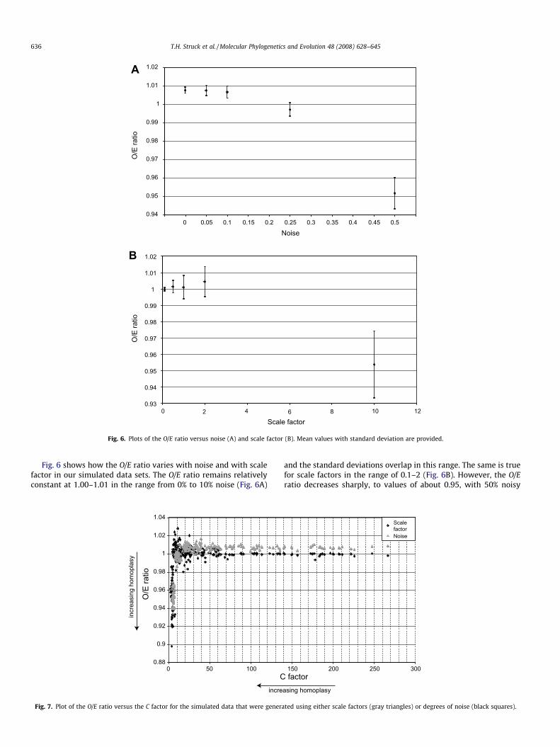
Fig. 6 shows how the O/E ratio varies with noise and with scalefactor in our simulated data sets. The O/E ratio remains relativelyconstant at 1.00–1.01 in the range from 0% to 10% noise (Fig. 6A)

0.88

0.9

0.92

0.94

0.96

0.98

1

1.02

1.04

0 50 100C

O/E

ratio

incre

incr

easi

ng h

omop

lasy

Fig. 7. Plot of the O/E ratio versus the C factor for the simulated data that were genera

and the standard deviations overlap in this range. The same is truefor scale factors in the range of 0.1–2 (Fig. 6B). However, the O/Eratio decreases sharply, to values of about 0.95, with 50% noisy

150 200 250 300 factor

ScalefactorNoise

asing homoplasy

ted using either scale factors (gray triangles) or degrees of noise (black squares).


data or a 10-fold longer tree length. Given that the O/E ratio mea-sures the degree of homoplasy relative to the complete data set,such a result is not surprising in our simulated concatenated datasets. A partition with a high degree of homoplasy (e.g., 50% noise)can increase the O/E ratio of another partition even though this onehas substantial homoplasy itself (e.g., 25% noise). The addition ofthe first one increases the average homoplasy of the complete dataset while the degree of homoplasy in the other partition remainsunaltered by the addition. Thus, due to the addition of the first par-tition the O/E ratio of the other partition increases, because it is rel-atively less homoplasious in comparison to the new average degreethan before (see also Discussion).

Fig. 7 shows the relation of the C factor to the O/E ratio in oursimulated data sets. The C factor correlates positively and linearlywith the O/E ratio at lower values, when homoplasy is high (Fig.7). Overall, the figure shows that an increasing C factor indicatesan increasing O/E ratio. However, the correlation does not staylinear. The O/E ratio increases strongly, from 0.9 to 1, up to a Cfactor of 10 and then it levels off. At a C factor of 20 and abovethe O/E ratio has a constant value of 1 or slightly higher. The va-lue of the C factor declines more sharply with increasing homo-plasy (scale or noise) than does the O/E ratio, as is obvious fromcomparing Figs. 5 and 6. More specifically, C starts declining atfar lower levels of homoplasy (>0 in Fig. 5) than does O/E (>10%or >2 in Fig. 6). Thus, C is a much more sensitive indicator ofhomoplasy. However, both C factor and O/E ratio correlate withhomoplasy and with each other when the degree of homoplasyincreases.

3.2. Classes of identity in the annelid example

The aligned, empirical, data set contained 2565 positions for the18S and 5775 for the 28S partition, from which GBlocks excluded1345 and 3429 ambiguously aligned positions, respectively. Inthe final alignment of 3566 positions 1368 positions were parsi-mony-informative, 1684 constant and 514 sites parsimony unin-formative. In the sliding window analyses, 10% increments ofvariability could be determined ranging from 0–80% in the 18S par-tition and from 0–100% in the 28S partition. In both, most positionswere within the classes of identity with low variability (Table 2: 0–10%, 10–20%, etc.) and higher classes of variability contain progres-sively fewer characters. The last two increments of the 28S parti-tion (80–90% and 90–100%) were pooled, because the latter onewould have had only 28 positions, which is a rather small samplesize for the calculations of the C factor and O/E ratio. That is, toosmall a sample size would produce too much random error.

The complete data partitions (‘‘ALL”), as well as every class ofidentity within partitions, showed homogeneity of base frequen-cies across taxa (Table 2).

Table 2Homogeneity of base frequencies and ANOVA results for the genetic distance p of the clas

Classes of identity Number of alignable characters Homogeneity of base freque

18S 28S 18S 28S

All 1220 2346 1.00 0.990–10% 250 432 1.00 1.0010–20% 251 431 1.00 1.0020–30% 209 435 1.00 1.0030–40% 138 269 1.00 1.0040–50% 133 224 1.00 1.0050–60% 99 209 1.00 1.0060–70% 87 139 1.00 1.0070–80% 53 104 1.00 1.0080–100% n.a. 103 n.a. 0.99

Significant values are in bold. n.a., not applicable.

Finally, we checked if either two neighbouring classes of iden-tity within a partition (e.g., 0–10% with 10–20% within the 18S par-tition) or the same classes of identity of two partitions (e.g., 0–10%of 18S and 28S partitions) had to be merged with each other, be-cause their characters were drawn from the same underlying prob-ability distribution. To the contrary ANOVA indicated that thecharacters of each class of identity were drawn from independentunderlying probability distributions and thus no classes have beenmerged (see the right side of Table 2). This means that the distribu-tion of genetic distances of pairwise-taxa comparisons was uniquefor each class of identity and never similar or identical to the dis-tribution of another one. This holds even though the mean-geneticdistances of some classes of identity are very similar (see thepoints that nearly touch in Fig. 8).

3.3. Detection of saturation in the annelid example

Fig. 8A shows how the C factor varies with increasing geneticdistance across annelid taxa in our empirical example. Withincreasing genetic distance the C factor decreases following apower function. Classes of identity from 0–30% for the 28S andfrom 0–20% for the 18S achieve values of more than 100, whereasclasses above 70% show values below 10 accompanied by muchhigher genetic distances. Thus, there is a difference of an order ofa magnitude. This resembles the results of our simulation studies,which exhibited a strong decrease of the C factor with increasinghomoplasy. Hence, the higher the variability in the class of identitythe stronger is the degree of saturation indicated by the C factor.

Turning to O/E ratio, all classes of identity in the 18S with de-grees of variation below 60%, as well as in the 28S below 50%, haveratios larger than or close to 1, whereas all other classes have val-ues below 1 (Fig. 8B). Generally, O/E ratio decreases with increasingvariability. However, while the classes of identity of the 18S in therange from 0–50% degree of variation remain more or less constantthe classes of the 28S exhibit an optimum of the O/E ratio in theclass of 20–30% variability.

The relation of the C factor to the O/E ratio is similar to our sim-ulation studies (Fig. 8C). The O/E ratio increases sharply up to 1 (orslightly higher) at low C factors and then starts to level off at C fac-tors in the range from 20 to 30. At higher C factors the O/E ratiomight be viewed as levelling off at a value around 1.01, exceptfor two maverick points for 28S. Furthermore, all six classes ofidentity possessing an O/E clearly smaller than 1 have a C factorequal to or smaller than 20, whereas nearly all others have a Cabove 20 (Fig. 8C). The lowest O/E value can be observed in theclass of identity 80–100% of the 28S partition, which has also thelowest C factor (Fig. 8A and B).

We decided to treat all classes of identity with an O/E ratioclearly below 1 (i.e., 0.99) as saturated, for three objective reasons.

ses of identity of 18S and 28S

ncies ANOVA results for the genetic distance p

18S vs. 28S Comparison 18S 28S

All <0.001 <0.0010–10% <0.001 0–10% vs. 10–20% <0.001 <0.001

10–20% <0.001 10–20% vs. 20–30% <0.001 <0.00120–30% <0.001 20–30% vs. 30–40% <0.001 <0.00130–40% <0.001 30–40% vs. 40–50% <0.001 <0.00140–50% <0.001 40–50% vs. 50–60% <0.001 <0.00150–60% <0.001 50–60% vs. 60–70% <0.001 <0.00160–70% <0.001 60–70% vs. 70–80% <0.001 <0.00170–80% 0.005 70–80% vs. 80–100% n.a. <0.001

80–100% n.a.

0

50

100

150

200

250

300

0.00 0.05 0.10 0.15 0.20 0.25 0.30 0.35

18S28S

Power

C fa

ctor

0.91

0.94

0.97

1

1.03

1.06

0 0.05 0.1 0.15 0.2 0.25 0.3 0.35

O/E

ratio

uncorrected genetic distance p

0-10%

10-20%

20-30%

30-40%

40-50% 50-60% 60-70% 70-80%80-100%

0-10%10-20%

20-30% 30-40%40-50%

50-60% 60-70% 70-80%

80-100%

0.94

0.95

0.96

0.97

0.98

0.99

1.00

1.01

1.02

1.03

1.04

0 5 0 100 150 200 250 300C factor

O/E

ratio

uncorrected genetic distance p

Fig. 8. Plots of both the C factor (A) and the O/E ratio (B) versus the genetic distance p for the actual data set, as well as a plot of the O/E ratio versus the C factor (C), all for theempirical data. The classes of identity of the 18S (black diamonds) and 28S (black squares) are indicated in the plots. In (A), the power function of the C factor is shown.


First, an O/E ratio below 1 indicates that the degree of homoplasy inthis class of identity is worse than the average degree in the com-plete data set. Second, given the relation of C factor and O/E ratio(Figs. 7 and 8C) the asymptote of the O/E ratios was in the rangefrom 1.00 to 1.01. Third, as mentioned in the previous paragraph,all O/E ratios with values clearly below 1 were generally accompa-nied by low C factors of 20 or less (Figs. 8C and 7). This means weeliminated in the saturation-excluded EX data set all classes of

identity with a degree of variation above 60% and also the classof identity 50–60% of the 28S. Such a strict and conservative proce-dure is similar to the one used by Struck et al. (2007).

3.4. Comparison of 28S fragments

Of the three 28S fragments that have been employed in the lit-erature, the D9/10 of annelids has a C factor of about 100, the

Table 3Comparison of the three different 28S fragments used in annelid phylogeny

Fragment C factor O/E ratio Genetic distance p

With s.c. Without s.c. With s.c. Without s.c. With s.c. Without s.c.

D1 (0.3 kb) 9.86 51.46 0.97 1.01 0.1357 0.04772.2 kb 15.66 64.77 0.93 1.06 0.1010 0.0508D9/10 (0.6 kb) 103.77 159.80 1.03 1.03 0.0382 0.0269

s.c., saturated characters.


2.2 kb fragment has a C factor around 15, and D1 has a C factoraround 10 (Table 3 with s.c.). Deleting supposedly saturated posi-tions increases the C factor in all three fragments. In fact, the Cfactors for the 2.2 kb and D1 fragments increase markedly, by afactor of 4–5. The O/E ratio of D9/10 is above 1 and is unalteredby the exclusion of saturated positions (Table 3). On the otherhand, the O/E ratios of the other two fragments are below 1and deleting saturated characters from these fragments increasestheir O/E ratios to above 1. This effect is most marked for the2.2 kb fragment, where an O/E ratio of 0.93 increases to 1.06. Inany case, we have found a way to assure O/E ratios are aboveour threshold of 1, for all three fragments and therefore to mini-mize homoplasy.

3.5. Phylogenetic analyses of the annelid example

For the annelid example of nearly complete 18S and 28S data,two data sets were analyzed, a complete one with only ambigu-ously aligned positions excluded, but saturated positions retained(ALL) and another one with the possibly saturated positions alsoexcluded (EX). ML analyses of both data sets were conducted intwo ways; that is, by using starting trees obtained by random tax-on addition, and by using the best tree of the BI as a starting tree. Inboth cases, the tree obtained using the best BI tree achieved a bet-ter (smaller) �ln L value than did the standard procedure of ran-dom taxon addition. Precisely, for the EX data set, �ln L usingrandom taxon addition was 31,647.03318 and using the best BItree 31,643.88339. For the ALL data, the values were62,622.70950 and 62,612.01527, respectively. Thus, for taxon-richdata sets its seems more promising to use near optimal startingtrees obtained by other procedures such as BI to increase the prob-ability to reconstruct the overall most likely tree. Additionally,such a tree search needed only about one third of the CPU timein our analyses.

Analyses excluding possibly saturated characters (EX) had justfour nodes showing zero branch length (Fig. 9) and the analysesnot excluding these characters (ALL) had only one (Fig. 10). Thus,overall the resolution in the trees is good, but support is low be-yond the ‘‘family” level in both. This is indicated by the paucityof support symbols on the basal nodes along the ‘‘backbones” (leftside) of the trees. Thirty-eight of the 104 internal nodes of the EXdata set exhibited maximum-parsimony-bootstrap support (MP-BS) P 70, and for 32 of these nodes the MP-BS were P95. Similarvalues were obtained for neighbor-joining bootstrapping (NJ-BS):38 nodes with NJ-BS P70 and 31 nodes P95. Forty-five of theinternal nodes had Bayesian posterior probabilities (PP) P0.95. Fi-nally, 40 nodes had a maximum-likelihood-bootstrap support (ML-BS) P70, and 32 of these were P95. In analyses of the ALL data set,47 nodes had MP-BS values P70, and 41 were P95. Fifty-twonodes exhibited ML-BS P70, and 40 of these nodes were P95.Similar results were obtained for NJ-BS and PP values: 47 nodesP70, 35 nodes P95 and 64 P 0.95, respectively. Thus, the ALL data(with more characters) consistently yielded more supported nodesthan did the EX data (with fewer characters), meaning that supportand resolution increased with the number of nucleotide positions.

Comparing the two trees (Figs. 9 and 10) reveals that for both datasets these support values favor more recent events and are not ran-domly spread out.

For both data sets, only a few taxa beyond the recognized ‘‘fam-ily” level are supported significantly as indicated by bootstrap val-ues. Monophyly of Aphroditiformia as well as of Clitellata issubstantiated. The close relationships of Echiura and Capitellidaeand of Eunicidae and Onuphidae (Bleidorn et al., 2003a, 2003b;Struck et al., 2006, 2007) are significantly corroborated. Addition-ally, in the analyses of the ALL data set (Fig. 10), monophyly ofTerebelliformia excluding Pectinariidae achieves significant sup-port by ML-BS and MP-BS as does the close relationship of Spioni-dae, Trochochaetidae and Poecilochaetidae. These resultscorroborate previous findings (e.g., Bleidorn et al., 2003b; Colganet al., 2006; Rousset et al., 2007; Struck and Purschke, 2005; Strucket al., 2007; Worsaae et al., 2005).

For this study we also obtained new 18S and/or 28S data forsome polychaete taxa. Our analyses allow tentative conclusionsregarding some of these taxa. Both analyses (Figs. 9 and 10)grouped Spionidae, Trochochaetidae and Poecilochaetidae to-gether. This clade gathered significant support in the analysesusing ALL data (Fig. 10). This result is in agreement with morpho-logical data, which place these taxa in Spionida (Rouse and Fauch-ald, 1997; Rouse and Pleijel, 2001). On the other hand, the otherspionidan taxon for which we obtained new data, Apistobranchi-dae, is sister to the sabellidan taxon Oweniidae in both analyses(Figs. 9 and 10). In this study coverage of Opheliidae was increasedin comparison to recent studies (Colgan et al., 2006; Struck et al.,2007) and Opheliidae were recovered as sister(s) to Clitellata, al-beit with weak support (Figs. 9 and 10). This was also found inan analysis based on 18S data alone (Struck et al., 2005). Mostnew sequences were obtained for the former archiannelidan taxaDinophilidae, Nerillidae, Polygordiidae, Protodrilidae, Protodriloi-dae, and Saccocirridae (see Hermans, 1969). Monophyly of the‘‘Archiannelida” has been rejected based on morphological andmolecular data (Purschke and Jouin, 1988; Struck et al., 2005,2002a,b; Westheide, 1997), which is further substantiated by ourresults (Figs. 9 and 10). Monophyly of the morphologically well-de-fined taxon Protodrilida comprising Protodrilidae, Protodriloidae,and Saccocirridae (Purschke and Jouin, 1988; Rouse and Pleijel,2001) was also not recovered by our analyses (Figs. 9 and 10). Thisis congruent with results mainly derived from 18S data (Hall et al.,2004; Rousset et al., 2007; Struck et al., 2002a; Struck and Purs-chke, 2005).

3.6. Number of positions

Because our larger ALL data set with more positions (Fig. 10)gave better resolution than our smaller EX data set with fewerpositions, we used simulations to explore the effect of number ofpositions on the quality of tree reconstructions, with simulationsettings derived from a smaller, 10-taxon annelid example. Therelation of number of positions to saturation, recovery of the truetree, and phylogenetic method employed was investigated usingsimulated data sets with 100 up to 5000 positions. (Note that there

Fig. 9. Cladogram of the ML tree excluding possibly saturated positions (EX) leaving 2871 total positions. �lnL = 31,643.88339. Support values are indicated at the branches.Model parameters: base frequencies: A = 0.2659, C = 0.2057, G = 0.2943, T = 0.2341; substitution rates: A M C = 1.3007, A M G = 3.0178, A M T = 1.2128, C M G = 0.8623,C M T = 6.8312, G M T = 1.0000; a = 0.4900, number of categories = 4; proportion of invariant sites = 0.3810. A phylogram, indicating the actual branch length, is provided inSupplementary Figure 1.


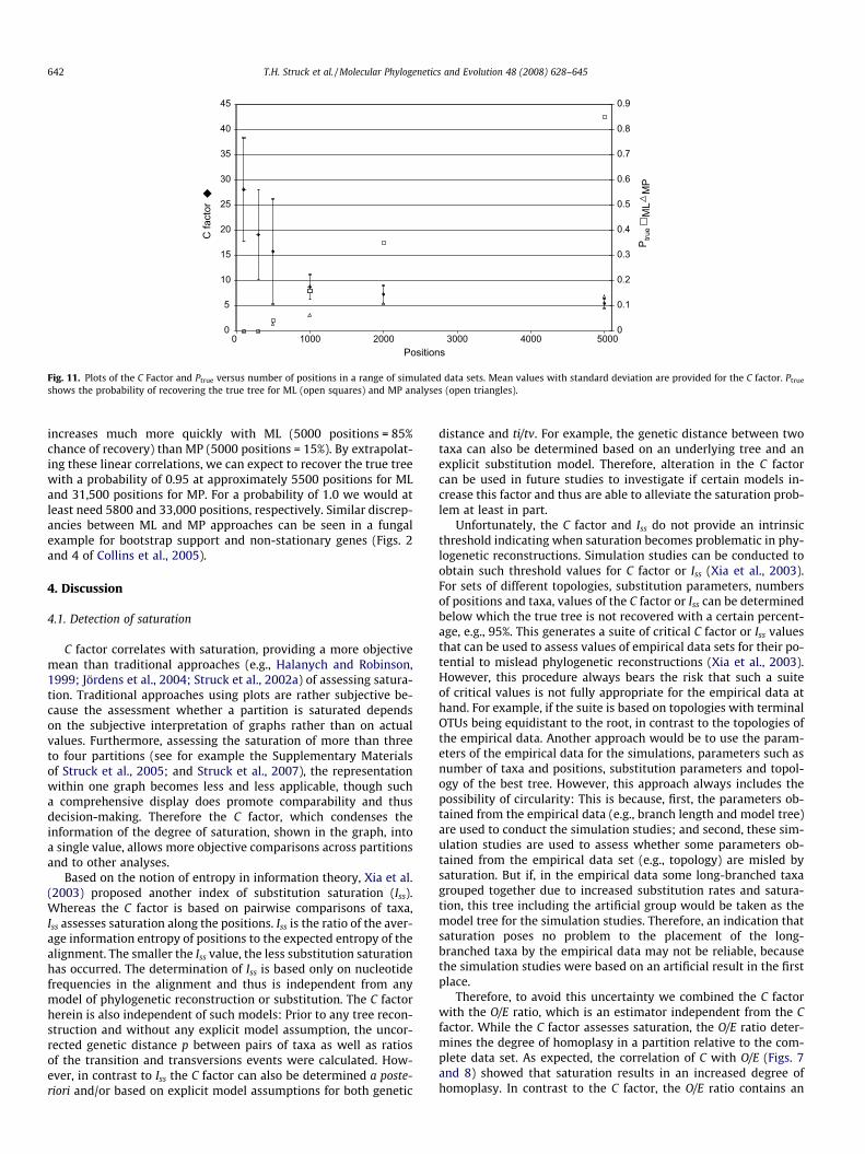
was no deliberately introduced noise this time; the different-sizeddata sets were increases in constant quality.) With an increasingnumber of positions, the C factor slightly decreases (Fig. 11). On

the other hand, recovery of the true tree (Fig. 1) increases withan increasing number of positions even though the C factor indi-cates that saturation is increasing (Fig. 11).

Fig. 10. Cladogram of the ML tree not excluding possibly saturated positions (ALL) with 3566 total positions. �lnL = 62,612.01527. That is, this is from a larger data set.Support values are indicated at the branches. Model parameters: base frequencies: A = 0.2410, C = 0.2331, G = 0.3008, T = 0.2251; substitution rates: A M C = 0.9835,A M G = 2.3338, A M T = 1.1084, C M G = 0.8864, C M T = 4.8116, G M T = 1.0000; a = 0.5726, number of categories = 4; proportion of invariant sites = 0.3803. A phylogram,indicating the actual branch length, is provided in Supplementary Figure 2.


However, the chance of recovering the true tree depends on thereconstruction method used. Neither ML nor MP recovers the truetree with only 100 or 300 positions. Starting with 500 characters,

the chance of recovering the true tree increases linearly withincreasing number of positions for both ML and MP (R2 for ML is0.997 and 0.826 for MP). Probability of recovering the true tree

0

5

10

15

20

25

30

35

40

45

0 1000 2000 3000 4000 50000

0.1

0.2

0.3

0.4

0.5

0.6

0.7

0.8

0.9

C fa

ctor

Ptru

e

Positions

MP

ML

Fig. 11. Plots of the C Factor and Ptrue versus number of positions in a range of simulated data sets. Mean values with standard deviation are provided for the C factor. Ptrue

shows the probability of recovering the true tree for ML (open squares) and MP analyses (open triangles).


increases much more quickly with ML (5000 positions = 85%chance of recovery) than MP (5000 positions = 15%). By extrapolat-ing these linear correlations, we can expect to recover the true treewith a probability of 0.95 at approximately 5500 positions for MLand 31,500 positions for MP. For a probability of 1.0 we would atleast need 5800 and 33,000 positions, respectively. Similar discrep-ancies between ML and MP approaches can be seen in a fungalexample for bootstrap support and non-stationary genes (Figs. 2and 4 of Collins et al., 2005).

4. Discussion

4.1. Detection of saturation

C factor correlates with saturation, providing a more objectivemean than traditional approaches (e.g., Halanych and Robinson,1999; Jördens et al., 2004; Struck et al., 2002a) of assessing satura-tion. Traditional approaches using plots are rather subjective be-cause the assessment whether a partition is saturated dependson the subjective interpretation of graphs rather than on actualvalues. Furthermore, assessing the saturation of more than threeto four partitions (see for example the Supplementary Materialsof Struck et al., 2005; and Struck et al., 2007), the representationwithin one graph becomes less and less applicable, though sucha comprehensive display does promote comparability and thusdecision-making. Therefore the C factor, which condenses theinformation of the degree of saturation, shown in the graph, intoa single value, allows more objective comparisons across partitionsand to other analyses.

Based on the notion of entropy in information theory, Xia et al.(2003) proposed another index of substitution saturation (Iss).Whereas the C factor is based on pairwise comparisons of taxa,Iss assesses saturation along the positions. Iss is the ratio of the aver-age information entropy of positions to the expected entropy of thealignment. The smaller the Iss value, the less substitution saturationhas occurred. The determination of Iss is based only on nucleotidefrequencies in the alignment and thus is independent from anymodel of phylogenetic reconstruction or substitution. The C factorherein is also independent of such models: Prior to any tree recon-struction and without any explicit model assumption, the uncor-rected genetic distance p between pairs of taxa as well as ratiosof the transition and transversions events were calculated. How-ever, in contrast to Iss the C factor can also be determined a poste-riori and/or based on explicit model assumptions for both genetic

distance and ti/tv. For example, the genetic distance between twotaxa can also be determined based on an underlying tree and anexplicit substitution model. Therefore, alteration in the C factorcan be used in future studies to investigate if certain models in-crease this factor and thus are able to alleviate the saturation prob-lem at least in part.

Unfortunately, the C factor and Iss do not provide an intrinsicthreshold indicating when saturation becomes problematic in phy-logenetic reconstructions. Simulation studies can be conducted toobtain such threshold values for C factor or Iss (Xia et al., 2003).For sets of different topologies, substitution parameters, numbersof positions and taxa, values of the C factor or Iss can be determinedbelow which the true tree is not recovered with a certain percent-age, e.g., 95%. This generates a suite of critical C factor or Iss valuesthat can be used to assess values of empirical data sets for their po-tential to mislead phylogenetic reconstructions (Xia et al., 2003).However, this procedure always bears the risk that such a suiteof critical values is not fully appropriate for the empirical data athand. For example, if the suite is based on topologies with terminalOTUs being equidistant to the root, in contrast to the topologies ofthe empirical data. Another approach would be to use the param-eters of the empirical data for the simulations, parameters such asnumber of taxa and positions, substitution parameters and topol-ogy of the best tree. However, this approach always includes thepossibility of circularity: This is because, first, the parameters ob-tained from the empirical data (e.g., branch length and model tree)are used to conduct the simulation studies; and second, these sim-ulation studies are used to assess whether some parameters ob-tained from the empirical data set (e.g., topology) are misled bysaturation. But if, in the empirical data some long-branched taxagrouped together due to increased substitution rates and satura-tion, this tree including the artificial group would be taken as themodel tree for the simulation studies. Therefore, an indication thatsaturation poses no problem to the placement of the long-branched taxa by the empirical data may not be reliable, becausethe simulation studies were based on an artificial result in the firstplace.

Therefore, to avoid this uncertainty we combined the C factorwith the O/E ratio, which is an estimator independent from the Cfactor. While the C factor assesses saturation, the O/E ratio deter-mines the degree of homoplasy in a partition relative to the com-plete data set. As expected, the correlation of C with O/E (Figs. 7and 8) showed that saturation results in an increased degree ofhomoplasy. In contrast to the C factor, the O/E ratio contains an


intrinsic threshold value of 1. Values above 1 indicate that the par-tition is less homoplasious than the average of the complete dataset and values below 1 that it is more homoplasious. In our analy-ses, O/E values clearly below 1 corresponded with a C factor below10, and C factors in the range of 10–20 were associated with O/Eratios below or close to 1 (Fig. 7 and 8C). At higher C values, theO/E ratio leveled off. Therefore, the critical threshold of the C factormay be in the range of 10–20, because this is where the drop-off ofthe O/E ratio occurred.

However, this range and the correlation between C and O/Eshould be further investigated by employing a wide variety ofempirical data. Although the degrees of homoplasy and saturationare correlated in the present study, this might not hold up in all in-stances. For example, a data set showing no or only slight satura-tion can still exhibit some homoplasy if there are numerousparallel mutations, as might occur under strong selection. Thus,there will be O/E values below 1 in parts of such a data set, withoutindicating saturation. Conversely, if a data sets shows saturationoverall, some parts of it will still have a O/E ratio above 1 amongthe many classes of identity. Moreover, because the O/E ratio is arelative measure to the degree of homoplasy of the complete dataset, there will always be values above and below 1. Additionally, ifa single class of identity covers all positions of a data set, the aver-age of O/E ratios of the ‘‘classes” of identity is 1. Thus, the relativeO/E ratio can only be used as an additional, supportive measure-ment for saturation in combination with direct factors such asthe C factor. For the annelid ribosomal data, we excluded all parti-tions with an O/E value below 1 from the subsequent phylogeneticanalysis. Given these arguments, this cut-off point might have beenoverly conservative, though the values correlated with low C fac-tors below 20.

O/E ratio is valuable not only for comparing possibly saturatedcharacters, but also for assessing the quality of different data par-titions in a concatenated analysis in terms of degree of homoplasy:The smaller the O/E ratio of a partition, the more homoplasy it con-tains (in comparison to the complete data set and other partitionsin the analysis). Because it is a parsimony measurement and it iscalculated using CIs, the O/E ratio can directly compare differenttypes of characters such as amino acid, nucleotide and morpholog-ical traits, within one data set and one approach. Furthermore, incontrast to only using CIs of individual partitions, O/E ratios can tellhow CIs are altered when positions are deleted or added. Alterationapproaches are able to reveal not only contributions of individualpartitions, but also their influence on other partitions in the dataset (e.g., Gatesy et al., 1999; Struck, 2007).

4.2. Possibly saturated positions and Annelida phylogeny

Though exclusion of possibly saturated positions can improvephylogenetic reconstructions (e.g., Simon et al., 1994), this ap-proach seems not be helpful for the reconstruction of the annelidphylogeny using 18S and 28S sequence data. Instead, we foundthat using more positions (3566 nt, Fig. 10, ALL) was better thanusing fewer by excluding some (2871 nt, Fig. 9, EX). That is, bothnodal support and tree resolution increased with increasing num-ber of positions (cf. Figs. 9 and 10). Our EX analyses showed resultssimilar to previous analyses (e.g., Colgan et al., 2006; Rousset et al.,2007; Struck and Purschke, 2005), with low resolution and para-phyly of many clades – even of clades that are well-supported byanatomical characters, such as Phyllodocida and Eunicida (Fig. 9).On the other hand, though the support is still weak, analyses basedon the ALL data set (Fig. 10) showed some progress in comparisonto the ones based on EX. Some of the clades recovered in this ALLtree have also been found by Struck et al. (2007) and/or are sup-ported by morphological data. The analyses of Struck et al.(2007) used three nuclear genes and included nearly complete

18S and 28S, but excluded possibly saturated positions. These anal-yses were based on roughly the same number of parsimony-infor-mative characters as the ALL analyses in the present study. Forexample, Struck et al. (2007) also recovered a clade comprisingall Phyllodocida, Eunicida and Orbiniidae, albeit given low support(Fig. 10). Unlike the earlier analysis, this analysis (Fig. 10) also in-cludes Parergodrilidae, and places this taxon in the clade as well; inagreement, a close relationship of Orbiniidae and Parergodrilidaehas been shown previously (Bleidorn et al., 2003a; Erséus and Kal-lersjo, 2004; Jördens et al., 2004; Struck et al., 2002a). As recoveredhere, Struck et al. (2007) found a monophyletic Terebelliformia andbasal positions of Amphinomida and Chaetopteridae, but againwith low support. Basal Chaetopteridae has also been shown inthe analyses of Colgan et al. (2006). Our and the analyses of Strucket al. (2007) recovered with low support part of Spionida as being asubgroup of paraphyletic Sabellida. Our analyses based on ALL datarecovered Cirratuliformia with low support, a group proposed byRouse and Fauchald (1997).

The conclusion that adding more positions outweighs the im-pact of reducing saturation in annelid phylogeny in this study isfurther substantiated by the simulation studies (Fig. 11), whichwere based on actual substitution parameters of annelid taxa. Withan increasing number of positions, recovery of the true tree in-creases tremendously using ML methods, which is superior toMP in reconstructing annelid phylogeny. This agrees with previousstudies showing the general superiority of ML methods over MPmethods in reconstructing difficult trees—because ML can accountfor multiple substitutions at a site (e.g., Gadagkar and Kumar,2005; Hall, 2005; Huelsenbeck, 1995). With more than 5000 posi-tions modeled for the 18S and 28S sequences, the ‘true’ phylogenyof the 9 annelid OTUs can be recovered with high certainty usingML (right side of Fig. 11). Thus, for small numbers of annelid taxa,the ‘true’ phylogeny can be recovered with high certainty usingfewer than 10,000 positions (though the nodal support might stillbe weak). However, with increasing numbers of taxa, the amountof positions needed to recover the ‘true’ phylogeny with high cer-tainty will likewise increase. (Note that although these consider-ations are valuable in showing that more sites yield betterresolution, they are only of limited practical value because the nu-clear rRNA-gene family has only about 5400 usable sites, and thisnumber cannot be increased.)

Our results of empirical and simulated data showed thatincreasing the amount of nucleotide positions outweighed the neg-ative impact of saturated positions in the reconstruction of annelidphylogeny using nuclear rRNA data. Similar results have been ob-tained for a plastid gene in land plants and mitochondrial genesin birds (Crowe et al., 2006; Källersjö et al., 1999; Nickrent et al.,2000). In other studies, the third codon positions of protein-codinggenes have been especially problematic due to saturation (Grayb-eal, 1993; Halanych and Robinson, 1999; Xia et al., 2003). Third co-don positions of mitochondrial genes in annelids exhibit highmean-genetic distances, of about 0.6 (see Supplementary Materialin Struck et al., 2007). This means that 60% of the third codon posi-tions are different between any two annelid taxa. Additionally,these third codon positions do not show homogeneity of base fre-quencies across taxa (Supplementary Material in Struck et al.,2007). Thus, these positions begin to approximate random data.Therefore, neither should saturated positions be excluded a prioribefore any phylogenetic analysis of these positions nor shouldone fail to investigate saturation entirely, but the effect of satura-tion on the phylogenetic reconstruction should be assessed foreach data set anew. The C and O/E factors provided here may helpto guide the decision more objectively.

Finally, increasing the number of characters will not alwayshelp. For example, ambiguously aligned positions should alwaysbe excluded from the data set a priori, because robust hypothesis


about positional homology are important. Positional homology isthe fundamental principal in phylogenetic analyses at the se-quence level of nucleotides or amino acids and thus its violationhas strong impacts on both the reconstruction procedure itselfand its philosophical underpinnings (Swofford et al., 1996).

4.3. Comparison of 28S fragments

Given the above considerations about sequence length, whenworking with 28S data, it is preferable to use the nearly completesequence than just small chunks of the gene. Of the three differentfragments used in annelid phylogeny the D9/10 fragment is best inhaving the least genetic distance and the highest C factor (Table 3).Furthermore, the O/E ratio is clearly above 1 and is not tremen-dously altered due to the exclusion of possibly saturated positions.Thus, this fragment seems not be hampered by saturation.

The 2.2 kb fragment, on the other hand, has the benefits ofbeing longer and of achieving the best O/E ratio after exclusion ofpossibly saturated positions. On the other hand, before removalof its saturated characters, this fragment has the worst O/E ratiowith 0.93. Thus, the degree of homoplasy of this fragment isstrongly influenced by those partitions in it that have low C factorsand thus, saturated characters. This strong impact might be due tothe fact that this 2.2 kb fragment contains the large D2, D3, and D8divergence domains, which are highly variable and homoplasious(THS and KMH pers. obs. and see Hassouna et al., 1984; Hillisand Dixon, 1991; Mallatt et al., 2001; Zardoya and Meyer, 2001).Furthermore, the marked increase in the O/E ratio upon removingsaturated sites from the 2.2 kb piece shows the correlation of de-gree of homoplasy with the C factor: the higher the factor, the lessthe homoplasy.

The lowest C factor is achieved for the D1 fragment (Table 3). Itis below 10 and thus similar to the values of the classes of identityshowing clear saturation (Fig. 8). Furthermore, and in contrast tothe 2.2 kb fragment, the exclusion of possibly saturated charactersfrom D1 only raises the low O/E ratio slightly above 1, even thoughit discards more than half of the already small fragment of 0.3 kb(Brown et al., 1999). Additionally, the D1 fragment shows the high-est genetic distance (across taxa) of all fragments. The D1 fragmentis located at the 50 end of 28S rDNA and contains the D1 divergencedomain, which is like the D2, D3 and D8 divergence domainshighly variable and homoplasious in annelids (THS pers. obs.). Highsubstitution numbers in the D1 domain have also been shown forvertebrates as well (Zardoya and Meyer, 2001). Therefore, the D1fragment is the least favorable one of the three in terms of bothsize and properties. The D9/10 fragment is superior to it in termsof properties and the 2.2 kb one in terms of size.

5. Conclusions

Herein we introduce the C factor, a better way to assess satura-tion than is plotting ti/tv ratios against genetic distances. Our re-sults showed that the C factor correlates with saturation as wellas homoplasy. To determine the amount of homoplasy in a parti-tion relative to that in the complete data set, we also developedthe O/E ratio. Both factors in combination allow a more objectiveway to decide whether or not positions are saturated and are thusmisleading the phylogenetic reconstruction. However, we alsoshowed using empirical and simulated data that the effect of satu-ration can be counterbalanced by increased numbers of nucleotidepositions if appropriate methods of phylogenetic reconstruction,such as ML, are used. For the annelid example employed here,based on recovered clades, nodal support and resolution, theincreasing number of positions is more beneficial for improvingtree resolution in phylogenetic reconstruction than is excluding

saturated positions. Therefore, with respect to 28S rDNA, usingnearly complete 28S sequences is preferable to using small chunksof the gene.

Acknowledgments

We thank Christoph Bleidorn, Monika C. Müller, Anna Pauland Katrine Worsaae for providing tissue material. The crewof the R/V Point Sur and R/V Oceanus were most helpful inobtaining samples. For both cruises, we also acknowledge thehelp of the scientific crews (which are too numerous to listhere). Friday Harbor Laboratories, University of Washington, isalso acknowledged for their support. Computational assistanceon GUMP (Genomics Using Multiple Processors) at Auburn Uni-versity was kindly provided by Scott Santos. We also thank twoanonymous reviewers for important contributions to the manu-script. This work was supported by the USA National ScienceFoundation (NSF) WormNet Grant (EAR-0120646) to K.M.H.,NSF OCE-0425060 to K.M.H. and T.H.S., and by the GrantDFG-STR-683/3-1 from the Deutsche Forschungsgemeinschaftto T.H.S. This work is AU Marine Biology Program contribution#37.

Appendix A. Supplementary data

Supplementary data associated with this article can be found, inthe online version, at doi:10.1016/j.ympev.2008.05.015.

References

Altekar, G., Dwarkadas, S., Huelsenbeck, J.P., Ronquist, F., 2004. Parallel Metropolis-coupled Markov chain Monte Carlo for Bayesian phylogenetic inference.Bioinformatics 20, 407–415.

Bartolomaeus, T., 1995. Structure and formation of the uncini in Pectinaria koreni,Pectinaria auricoma (Terebellida) and Spirorbis spirorbis (Sabellida): implicationsfor annelid phylogeny and the position of the Pogonophora. Zoomorphology115, 161–177.

Bleidorn, C., Podsiadlowski, L., Bartolomaeus, T., 2006. The complete mitochondrialgenome of the orbiniid polychaete Orbinia latreilli (Annelida, Orbiniidae)–anovel gene order for Annelida and implications for annelid phylogeny. Gene370, 96–103.

Bleidorn, C., Vogt, L., Bartolomaeus, T., 2003a. A contribution to sedentarypolychaete phylogeny using 18S rRNA sequence data. J. Syst. Zool. Evol. Res.41, 186–195.

Bleidorn, C., Vogt, L., Bartolomaeus, T., 2003b. New insights into polychaetephylogeny (Annelida) inferred from 18S rDNA sequences. Mol. Phylogenet. Evol.29, 279–288.

Bleidorn, C., Vogt, L., Bartolomaeus, T., 2005. Molecular phylogeny of lugworms(Annelida, Arenicolidae) inferred from three genes. Mol. Phylogenet. Evol. 34,673–679.

Brown, S., Rouse, G.W., Hutchings, P., Colgan, D., 1999. Assessing the usefulness ofhistone H3, U2 snRNA and 28S rDNA in analyses of polychaete relationships.Aust. J. Zool. 47, 499–516.

Castresana, J., 2000. Selection of conserved blocks from multiple alignments fortheir use in phylogenetic analysis. Mol. Biol. Evol. 17, 540–552.

Colgan, D.J., Hutchings, P.A., Braune, M., 2006. A multigene framework forpolychaete phylogenetic studies. Organisms Diversity & Evolution 6, 220–235.

Collins, T.M., Fedrigo, O., Naylor, G.J.P., 2005. Choosing the best genes for the job:the case for stationary genes in genome-scale phylogenetics. Syst. Biol. 54, 493–500.

Crowe, T.M., Bowie, R.C.K., Bloomer, P., Mandiwana, T.G., Hedderson, T.A.J., Randi, E.,Pereira, S.L., Wakeling, J., 2006. Phylogenetics, biogeography and classificationof, and character evolution in, gamebirds (Aves: Galliformes): effects ofcharacter exclusion, data partitioning and missing data. Cladistics 22, 495–532.

Erséus, C., 2005. Phylogeny of oligochaetous Clitellata. Hydrobiologia (535/536),357–372.

Erséus, C., Kallersjo, M., 2004. 18S rDNA phylogeny of Clitellata (Annelida). Zool. Scr.33, 187–196.

Fauchald, K., Rouse, G., 1997. Polychaete systematics: past and present. Zool. Scr. 26,71–138.

Gadagkar, S.R., Kumar, S., 2005. Maximum likelihood outperforms maximumparsimony even when evolutionary rates are heterotachous. Mol. Biol. Evol. 22,2139–2141.

Gatesy, J., O’Grady, P., Baker, R.H.(R.H., 1999. Corroboration among data sets insimultaneous analysis: hidden support for phylogenetic relationships amonghigher level artiodactyl taxa. Cladistics 15, 271–313.

http://dx.doi.org/10.1016/j.ympev.2008.05.015


Graybeal, A., 1993. The phylogenetic utility of cytochrome b: lessons from bufonidfrogs. Mol. Phylogenet. Evol. 2, 256–269.

Halanych, K.M., 2004. The new view of animal phylogeny. Annu. Rev. Ecol. Evol.Syst. 35, 229–256.

Halanych, K.M., Robinson, T.J.(T.J., 1999. Multiple substitutions affect thephylogenetic utility of cytochrome b and 12S rDNA data: examining a rapidradiation in leporid (Lagomorpha) evolution. J. Mol. Evol. 48, 369–379.

Hall, B.G., 2005. Comparison of the accuracies of several phylogenetic methodsusing protein and DNA sequences. Mol. Biol. Evol. 22, 792–802.

Hall, K.A., Hutchings, P.A., Colgan, D.J., 2004. Further phylogenetic studies of thePolychaeta using 18S rDNA sequence data. J. Mar. Biol. Ass. UK 84, 949–960.

Hassouna, N., Michot, B., Bachellerie, J.-P., 1984. The complete nucleotide sequenceof mouse 28S rRNA gene. Implications for the process of size increase of thelarge subunit rRNA in higher eukaryotes. Nucleic Acids Res. 12, 3563–3583.

Hermans, C.O., 1969. The systematic position of the Archiannelida. Syst. Zool. 18,85–102.

Hessling, R., 2002. Metameric organisation of the nervous system in developmentalstages of Urechis caupo (Echiura) and its phylogenetic implications.Zoomorphology 121, 221–234.

Hillis, D.M., Dixon, M.T., 1991. Ribosomal DNA: molecular evolution andphylogenetic inference. Q. Rev. Biol. 66, 411–453.

Huelsenbeck, J.P., 1995. Performance of phylogenetic methods in simulation. Syst.Biol. 44, 17–48.

Huelsenbeck, J.P., Ronquist, F., 2001. MRBAYES: Bayesian inference of phylogenetictrees. Bioinformatics 17, 754–755.

Jördens, J., Struck, T.H., Purschke, G., 2004. Phylogenetic inference regardingParergodrilidae and Hrabeiella periglandulata (‘‘Polychaeta”, Annelida) basedon 18S rDNA, 28S rDNA and COI sequences. Journal of Zoological Systematicsand Evolutionary Research 42, 270–280.

Källersjö, M., Albert, V.A., Farris, J.S., 1999. Homoplasy increases phylogeneticstructure. Cladistics 15, 91–93.

Kuhner, M.K., Felsenstein, J., 1994. A simulation comparison phylogeny algorithmsunder equal and unequal evolutionary rates. Mol. Biol. Evol. 11, 459–468.

Lake, J.A., 1994. Reconstructing evolutionary trees from DNA and proteinsequences: paralinear distances. Proc. Natl. Acad. Sci. USA 91, 1455–1459.

Lockhart, P.J., Steel, M.A., Hendy, M.D., Penny, D., 1994. Recovering evolutionarytrees under a more realistic model of sequence evolution. Mol. Biol. Evol. 11,605–612.

Lopez, P., Forterre, P., Philippe, H., 1999. The root of the tree of life in the light of thecovarion model. J. Mol. Evol. 49, 496–508.

Maddison, W.P., Maddison, D.R. 2004. Mesquite: a modular system for evolutionaryanalysis. Version 1.05. http://mesquiteproject.org.

Mallatt, J., Sullivan, J., Winchell, C.J., 2001. The relationship of lampreys to hagfishes:a spectral analysis of ribosomal DNA sequences. In: Ahlberg, P.E. (Ed.), MajorEvents in Early Vertebrate Evolution: Palaeontology, Phylogeny, Genetics, andDevelopment. Taylor & Francis, London, pp. 106–118.

McHugh, D., 1997. Molecular evidence that echiurans and pogonophorans arederived annelids. Proc. Natl. Acad. Sci. USA 94, 8006–8009.

McHugh, D., 2000. Molecular phylogeny of the Annelida. Can. J. Zool. 78, 1873–1884.

McHugh, D., 2005. Molecular systematics of polychaetes (Annelida). Hydrobiologia,309–318.

Milinkovitch, M.C., LeDuc, R.G., Adachi, J., Farnir, F., Georges, M., Hasegawa, M.,1996. Effects of character weighting and species sampling on phylogenyreconstruction: a case study based on DNA sequence data in Cetaceans.Genetics 144, 1817–1833.

Nicholas, K.B., Nicholas, H.B.J. 1997. GeneDoc: a tool for editing and annotatingmultiple sequence alignments. Distributed by the author.

Nickrent, D.L., Parkinson, C.L., Palmer, J.D., Duff, R.J., 2000. Multigene phylogeny ofland plants with special reference to bryophytes and the earliest land plants.Mol. Biol. Evol. 17, 1885–1895.

Nylander, J.A.A. (2002) MrModeltest. http://morphbank.ebc.uu.se/MR.BAYES.Pesole, G., Sbisà, E., Preparata, G., Saccone, C., 1992. The evolution of the

mitochondrial D-Loop and the origin of modern man. Mol. Biol. Evol. 9, 587–598.

Philippe, H., Forterre, P., 1999. The rooting of the universal tree of life is not reliable.J. Mol. Evol. 49, 509–523.

Posada, D., Buckley, T.R., 2004. Model selection and model averaging inphylogenetics: advantages of akaike information criterion and bayesianapproaches over likelihood ratio tests. Syst. Biol. 53, 793–808.

Posada, D., Crandall, K.A., 1998. MODELTEST: testing the model of DNA substitution.Bioinformatics 14, 817–818.

Posada, D., Crandall, K.A., 2001. Selecting the best-fit model of nucleotidesubstitution. Syst. Biol. 50, 580–601.

Purschke, G., 2002. On the ground pattern of Annelida. Org. Divers. Evol. 2, 181–196.Purschke, G., Jouin, C., 1988. Anatomy and ultrastructure of the ventral pharyngeal

organs of Saccocirrus (Saccocirridae) and Protodriloides (Protodriloidae fam. n.)

with remarks on the phylogenetic relationships within Protodrilida (Annelida:Polychaeta). J. Zool. 215, 405–432.

Regier, J., Shultz, J., 1997. Molecular phylogeny of the major arthropod groupsindicates polyphyly of crustaceans and a new hypothesis for the origin ofhexapods. Mol. Biol. Evol. 14, 902–913.

Ronquist, F., Huelsenbeck, J.P., 2003. MRBAYES 3: Bayesian phylogenetic inferenceunder mixed models. Bioinformatics 19, 1572–1574.

Rouse, G.W., Fauchald, K., 1997. Cladistics and polychaetes. Zool. Scr. 26, 139–204.Rouse, G.W., Pleijel, F., 2001. Polychaetes. University Press, Oxford.Rousset, V., Pleijel, F., Rouse, G.W., Erséus, C., Siddall, M.E., 2007. A molecular

phylogeny of annelids. Cladistics 23, 41–63.Simon, C., Frati, F., Beckenbach, A.T., Crespi, B., Liu, H., Flook, P., 1994. Evolution,

weighting, and phylogenetic utility of mitochondrial gene sequences and acompilation of conserved polymerase chain reaction primers. Ann. Entomol.Soc. Am. 87, 651–701.

Struck, T.H., 2007. Data congruence, paedomorphosis and salamanders. Front. Zool.4, 22.

Struck, T.H., Halanych, K.M., Purschke, G., 2005. Dinophilidae (Annelida) is mostlikely not a progenetic Eunicida: evidence from 18S and 28S rDNA. Mol.Phylogenet. Evol. 37, 619–623.

Struck, T.H., Hessling, R., Purschke, G., 2002a. The phylogenetic position of theAeolosomatidae and Parergodrilidae, two enigmatic oligochaete-like taxa of the‘Polychaeta’, based on molecular data from 18SrDNA sequences. J. Zool. Syst.Evol. Res. 40, 155–163.

Struck, T.H., Purschke, G., 2005. The sister group relationship of Aeolosomatidaeand Potamodrilidae (Annelida: ‘‘Polychaeta”)—a molecular phylogeneticapproach based on 18S rDNA and Cytochrome Oxidase I. Zool. Anz. 243,281–293.

Struck, T.H., Purschke, G., Halanych, K.M., 2006. Phylogeny of Eunicida (Annelida)and Exploring Data Congruence using a Partition Addition Bootstrap Alteration(PABA) approach. Syst. Biol. 55, 1–20.

Struck, T.H., Schult, N., Kusen, T., Hickman, E., Bleidorn, C., McHugh, D., Halanych,K.M., 2007. Annelida phylogeny and the status of Sipuncula and Echiura. BMCEvol. Biol. 7, 57.

Struck, T.H., Westheide, W., Purschke, G., 2002b. Progenesis in Eunicida(‘‘Polychaeta,” Annelida)—separate evolutionary events? Evidence frommolecular data. Mol. Phylogenet. Evol. 25, 190–199.

Sturmbauer, C., Meyer, A., 1992. Genetic divergence, speciation and morphologicalstasis in a lineage of African cichlid fishes. Nature 358, 578–581.

Swofford, D.L. 2002. PAUP*. Phylogenetic Analysis Using Parsimony (*and OtherMethods). Sinauer Associates, Sunderland, MA.

Swofford, D.L., Olsen, G.J., Waddell, P.J., Hillis, D.M., 1996. Chapter 11—phylogeneticinference. In: Hillis, D.M., Moritz, C., Mable, B.K. (Eds.), Molecular Systematics.Sinauer Associates, Sunderland, MA, pp. 407–514.

Thompson, J.D., Higgins, D.G., Gibson, T.J., 1994. CLUSTAL W: improving thesensitivity of progressive multiple sequence alignment through sequenceweighting, position-specific gap penalties and weight matrix choice. NucleicAcids Res. 22, 4673–4680.

Tzetlin, A., Purschke, G., 2006. Fine structure of the pharyngeal apparatus of thepelagosphera larva in Phascolosoma agassizii (Sipuncula) and its phylogeneticsignificance. Zoomorphology 125, 109–117.

Vogt, L., 2002. Testing and weighting characters. Org. Diversity Evol. 2, 319–333.Westheide, W., 1997. The direction of evolution within the Polychaeta. J. Nat. Hist.

31, 1–15.Westheide, W., McHugh, D., Purschke, G., Rouse, G., 1999. Systematization of the

Annelida: different approaches. Hydrobiologia 402, 291–307.Worsaae, K., Nygren, A., Rouse, G., Giribet, G., Persson, J., Sundberg, P., Pleijel, F.,

2005. Phylogenetic position of Nerillidae and Aberranta (Polychaeta, Annelida),analysed by direct optimization of combined molecular and morphologicaldata. Zool. Scr. 34, 313–328.

Wuyts, J., Van de Peer, Y., De Wachter, R., 2001. Distribution of substitution ratesand location of insertion sites in the tertiary structure of ribosomal RNA.Nucleic Acids Res. 29, 5017–5028.

Xia, X., Xie, Z., Salemi, M., Chen, L., Wang, Y., 2003. An index of substitutionsaturation and its application. Mol. Phylogenet. Evol. 26, 1–7.

Yang, Z., 1993. Maximum-likelihood estimation of phylogeny from DNA sequenceswhen substitution rates differ over sites. Mol. Biol. Evol. 10, 1396–1401.

Yang, Z., 1996. Among-site rate variation and its impact on phylogenetic analyses.Trends Ecol. Evol. 11, 367–372.

Zardoya, R., Meyer, A., 2001. Vertebrate phylogeny: limits of inference ofmitochondrial genome and nuclear rDNA sequence data due to an adversephylogenetic signal/noise ratio. In: Ahlberg, P.E. (Ed.), Major Events in EarlyVertebrate Evolution: Palaeontology, Phylogeny, Genetics, and Development.Taylor & Francis, London, pp. 135–155.

Zwickl, D.J., 2006. Genetic algorithm approaches for the phylogenetic analysis oflarge biological sequence datasets under the maximum likelihood criterion.Ph.D. dissertation., The University of Texas at Austin.

http://mesquiteproject.org

http://morphbank.ebc.uu.se/MR.BAYES

detecting possibly saturated positions in 18s and 28s sequences and their influence on phylogenetic...

Documents