detecting karenia brevis blooms and algal resuspension in the

Detecting Karenia brevis blooms and algal resuspension in the

western Gulf of Mexico with satellite ocean color imagery

Timothy T. Wynne a,*, Richard P. Stumpf a, Michelle C. Tomlinson a,Varis Ransibrahmanakul a, Tracy A. Villareal b

aNOAA, National Ocean Service, Center for Coastal Monitoring and Assessment, 1305 East West Highway, Silver Spring, MD 20910, USAbMarine Science Institute, The University of Texas at Austin, 750 Channel View Drive, Port Aransas, TX 78373, USA

Received 22 September 2004; received in revised form 2 February 2005; accepted 16 February 2005

Abstract

Blooms of the toxic dinoflagellate, Karenia brevis, have had detrimental impacts on the coastal Gulf of Mexico for decades.

Detection of Karenia brevis blooms uses an ecological approach based on anomalies derived from ocean color imagery. The

same anomaly product used in Florida produces frequent false positives on the Texas coast. These failures occurred during wind-

driven resuspension events. During these events resuspension of benthic algae significantly increases chlorophyll concentrations

in the water, resulting in confusion with normal water column phytoplankton, such as Karenia. A method was developed to

separate the resuspended chlorophyll from the water column chlorophyll, decreasing the false positives used with the detection

method.

# 2005 Elsevier B.V. All rights reserved.

Keywords: Anomaly; Chlorophyll; Gulf of Mexico; Harmful Algal Bloom; Karenia brevis; Remote sensing; Resuspension; SeaWiFS; Texas

www.elsevier.com/locate/hal

Harmful Algae 4 (2005) 992–1003

1. Background

Karenia brevis blooms are the principal cause of

Harmful Algal Blooms (HABs) in the Gulf of Mexico

(Kusek et al., 1999). K. brevis blooms cause massive

fish kills, marine mammal kills and respiratory

irritation in humans (Baden et al., 1995), and are

also known to cause Neurotoxic Shellfish Poisoning

(NSP) in various types of shellfish, which is hazardous

* Corresponding author. Tel.: +1 301 713 3028x139;

fax: +1 301 713 4388.

E-mail address: [email protected] (T.T. Wynne).

1568-9883/$ – see front matter # 2005 Elsevier B.V. All rights reserved

doi:10.1016/j.hal.2005.02.004

to humans. Because they have such toxic effects, K.

brevis blooms have been widely studied within the

Gulf of Mexico in order to improve detection and

monitoring. Tester et al. (1998) reported that the

eastern gulf (the west coast of Florida) had

experienced K. brevis blooms 26 out of the previous

27 years, and there has been a bloom reported every

year since 1998. Because of the frequency of blooms

on the west Florida shelf there has been an extensive

HAB monitoring program in place for years in that

region. For western portions of the gulf (the Texas

coastline), only three bloom events were reported

from 1935 to 1986. However, from 1986 to the

.

T.T. Wynne et al. / Harmful Algae 4 (2005) 992–1003 993

present, Texas had three documented major bloom

events in 1986, 1997 and 2000 (Magana et al., 2003)

and an apparently short lived (one positive cell count

reported in October at Brazos Santiago Pass and one

positive cell count in November at Sabine Pass) bloom

in October and November of 1999 (Villareal and

Magana, 2001). The change indicates that the

frequency and severity of Texas K. brevis blooms

may be increasing (Magana et al., 2003). There is no

regular monitoring by state agencies in Texas. The

limited sampling available outside of the bays is

research-driven and is not useful as an early warning

for K. brevis events. K. brevis cell count sampling in

the bays occurs in Texas only after a probable bloom

has been reported to the Texas Parks and Wildlife

Division (TPWD) or Texas Department of Health, and

sampling may occur only in economically important

areas, such as shellfish beds, so the number of Texas

blooms may be underestimated (Fig. 1).

1.1. History

Remote sensing techniques have been used to

investigate K. brevis since 1978, when remote sensing,

with an aircraft-based ocean color sensor, was first

shown to detect discoloration associated with a bloom

off the coast of southwest Florida (Muller, 1979).With

the launch of the Coastal Zone Color Scanner (CZCS)

in 1978, the potential has existed to detect HABs from

satellite observations. CZCS operated from November

1978 to June 1986, and was used by researchers to

examine K. brevis blooms during this time (Haddad,

1982). Since September 1997, when the Sea-viewing

Wide Field-of-view Sensor (SeaWiFS) became opera-

tional, near real time monitoring for Karenia has been

possible with ocean color satellite imagery. SeaWiFS,

ocean color data has become an important tool in

monitoring for K. brevis, including the ability to

provide alerts and forecasts to public health and

coastal resource managers through a regular produc-

tion of bulletins (Stumpf et al., 2003; Tomlinson et al.,

2004).

Satellite monitoring programs, such as the one

involved with SeaWiFS cannot be used to replace field

sampling programs, but can complement them. Field

sampling efforts incur tremendous costs in man hours

and ship time. Directing field sampling efforts to

dynamic areas that are likely to have a bloom or some

other oceanographic phenomenon would be advanta-

geous to managers and researchers. SeaWiFS is able to

detect such features on a regular basis with potential

daily revisits depending on cloud cover. SeaWiFS has

a nominal 1.1 km field of view (pixel size) and a swath

of over 2000 km in width allowing a synoptic view of

a relatively large area.

2. Methods

2.1. Standard anomaly method

Sea surface temperature (SST) anomalies have been

used to detect changes in the oceans, such as the

presence of an El Nino, upwelling events, and climate

predictions (Goddard et al., 2001). The change

detection concepts used for temperature anomalies

can also be employed with chlorophyll anomalies. The

Gulf of Mexico is an oligotrophic body of water, with a

relatively low background chlorophyll concentration.

When there is a bloom, a rapidly increasing concentra-

tion of phytoplankton, in the Gulf ofMexico, it is easily

seen in satellite imagery.This is because the chlorophyll

from a typical bloom, such as a Karenia bloom, can

have chlorophyll concentrations much higher than the

typical background concentrations.

SeaWiFS imagery was processed using the

SeaDAS 4 software. For atmospheric correction, the

chlorophyll algorithm of Stumpf et al. (2000) was

implemented, as it appears to give more consistent

results in the Gulf of Mexico. New chlorophyll

anomalies are then generated in order to detect

possible Karenia blooms. To determine the anomaly,

the mean chlorophyll is first determined for the 2

months ending 2 weeks before the current day

(Tomlinson et al., 2004). The current day SeaWiFS

image is then subtracted from this 2-month running

mean to create the anomaly, with positive anomalies

indicating a new phytoplankton bloom. The 2-week

lag between the 60-day mean and the current day

image is necessary in order to reduce the likelihood

that a persistent and stationary bloom will skew the

mean, and reduce the detection capability. Areas

within the resultant image that exhibit a change in

chlorophyll concentration greater than or equal to

1 mg L�1, during the K. brevis season, are considered

to be probable Karenia blooms. Exceptions are made

T.T. Wynne et al. / Harmful Algae 4 (2005) 992–1003994

Fig. 1. Map of the Texas coastline showing the study area.

in areas with significant river discharge, as these areas

rarely have Karenia blooms and frequently have

diatom blooms. Non-toxic algal blooms do occur in

this region and as a result field sampling is necessary

to positively identify the chlorophyll anomalies as

HABs. Other data, SSTand wind, is also used to refine

the detection (Stumpf et al., 2003). Tomlinson et al.

(2004) showed that along the panhandle and south-

western coasts of Florida, this method is about 80%

effective in recognizing K. brevis blooms during the

bloom season.

This same technique was then applied to the

western portion of the Gulf of Mexico but the initial

results were unsatisfactory, since there was an

abundance of anomalies for areas where no bloom

was reported. This discrepancy may be due to

infrequent in situ sampling in Texas (Villareal and

Magana, 2001), since event response sampling may

miss blooms that routine monitoring programs, such

as the one deployed in Florida, will catch. With the

absence of a routine monitoring system for Texas

waters, it is possible that blooms can occur and be

undetected. If a bloom occurs offshore in the presence

of offshore winds, dead fish and noxious aerosols will

not reach the shore, preventing the HAB event from

ever being documented. However, we presume,

conservatively, that anomalies occurring in a period

where no HAB is reported are false positives.


Many of the HAB anomalies coincided with

resuspension events along the Texas continental

shelf. The coastal waters of Texas have high

suspended sediment loads in the surface waters,

particularly in the northern portion of the state where

riverine runoff is high. Manheim et al. (1972) found

that the surface sediment load was still on the order

of 1 mg L�1. These are typical suspended sediment

loads, and can become significantly higher during

periods of extreme resuspension events. These

events can also transport benthic algae and sedi-

ments into the water column (Nelson et al., 1999).

Benthic chlorophyll that is resuspended to within

one optical depth of the surface will be detected by

satellite chlorophyll measurements and add to

existing planktonic chlorophyll concentrations. Total

benthic chlorophyll per unit area can exceed the

chlorophyll-a concentration in the integrated water

column (Radziejewska et al., 1996; Cahoon and

Laws, 1993; Cahoon et al., 1990). Therefore, during

resuspension events, benthic chlorophyll may dom-

inate the observed chlorophyll concentration. This

addition of resuspended benthic chlorophyll into the

system can produce a new chlorophyll anomaly

unrelated to the presence of K. brevis, a pelagic

dinoflagellate.

2.2. Corrected chlorophyll anomaly

In order to remove false positive HAB anomalies

caused by resuspended sediments, a method is

required to distinguish resuspended materials from

the chlorophyll-a concentrations that were present in

the water column prior to the resuspension event. To

do this we use more of the spectral information

available from SeaWiFS. The SeaWiFS sensor has

eight spectral bands. Six of these bands are in the

visible light spectrum, and are centered in the

following wavelengths: 412 nanometers (nm),

443 nm, 490 nm, 510 nm, 555 nm, 670 nm. The

remaining SeaWiFS bands lie in the near infrared

(NIR) and are used for atmospheric correction.

Backscattered light is directly correlated with the

concentration of inorganic sediments. For the sedi-

ment concentration levels found in this environment,

backscatter can be linearly approximated by the

reflectance in red wavelengths (Stumpf and Pennock,

1989).

Reflectance in the 670 nm band (R670), where

absorption is much greater than backscatter, can be

approximated by the following equation:

R670 /bb670

a670(1)

where bb670 and a670 are defined as the backscatter and

the absorption of the 670 nm band, respectively. Back-

scatter is defined by the following equation:

bb670 ¼ bbw þ bbs þ bbp (2)

where the subscripts of w, s, and p indicate contribu-

tions to backscatter from: water, sediment, and plank-

ton, respectively. The backscatter is related to

sediment concentration, S, by:

bbs ¼ bb0s � S (3)

where bb0s is the specific backscatter coefficient for

sediment.Absorption at 670 nm is defined as following:

a670 ¼ aw þ ag þ ad þ ap (4)

where the subscripts of w, g, d, and p indicate con-

tributions from: water, colored dissolved organic

material (CDOM), detritus, and plankton, respec-

tively. In general, aw � ag + ad + ap, and bbs � bbw+ bbp, so that reflectance is proportional to bbs/aw. By

combining this proportionality with Eq. (3), we see

that the red reflectance (R670) is a surrogate for sedi-

ment concentration (S). At shorter wavelengths, the

total absorption is not a constant, so reflectance cannot

be used to approximate the sediment concentration. As

the sediment load in the water column increases, the

reflectance in the 670 nm wavelength will increase.

In order to calculate a way to measure the amount

of resuspension in a given image, a 670 reflectance

anomaly is created, in the same way as the chlorophyll

anomaly described earlier. This method would flag

turbid river plumes as resuspension events. However,

the Texas coast has small plumes from its bays and

rivers, limiting this problem to periods after extensive

rains, tropical storms or hurricanes.

With a method in place to estimate the resuspension

at a given time and location, it becomes possible to

estimate the amount of chlorophyll that is introduced

into the water column as a result of resuspension

events. Benthic chlorophyll should resuspend at about

the same rate as sediment, so it was assumed that a


linear relationship exists between the chlorophyll

anomaly and the resuspended sediment anomaly. To

determine this relationship, several cloud free images

were selected, and a linear regression was calculated

between the 670 reflectance anomaly and the

chlorophyll anomaly for each image. The average

slope of the regression was approximately

200 mg sr L�1 and this slope was tested empirically

by comparing the effects that different regressions had

on imagery. The slope that yielded the most accurate

results was approximately 200 (Fig. 2). Therefore the

amount of resuspended benthic chlorophyll is esti-

mated as:

Resuspended Benthic Chlorophyll ðmgL�1Þ

¼ Rrs670ðsr�1Þ �M (5)

where M = Dchl/D670 = 200 mg sr L�1.

Subtracting this resuspended chlorophyll from the

total amount of chlorophyll in the system allows for an

estimate of how much chlorophyll was planktonic

during a resuspension event. However, for our

application, the difference of the chlorophyll anomaly,

which is the total ‘‘new’’ chlorophyll in the water and

the resuspended chlorophyll, gives the new planktonic

Fig. 2. Linear regression of the chlorophyll anomaly to the 670

reflectance anomaly for a single image. This relationship was used in

order to correct the chlorophyll anomaly for resuspension.

chlorophyll bloom through the adjusted chlorophyll

anomaly:

Adjusted Chl Anomaly ðmg L�1Þ

¼ Chl Anomaly ðmgL�1Þ

� Resuspended Benthic Chl ðmgL�1Þ (6)

3. Results and discussion

Visual analysis was performed on SeaWiFS images

from 1998 to 2002, both before and after the

resuspension correction was applied. The adjusted

chlorophyll anomaly method successfully removed

many of the unvalidated anomalies that were present

before the correction. There was a large and persistent

bloom of K. brevis documented in the summer/fall of

2000. This was the only documented major K. brevis

bloom during the time period of the study, and this

period was examined independently of the non-bloom

years. In non-bloom periods, 391 images were

examined and, 130 images or 33.2% had anomalies

before the correction. After the correction, 75 images,

or 19.1%, were flagged for blooms. The correction

eliminated 43% of the days containing anomalies. In

the 3-year period when there were no HABs reported,

there were no anomalies reported in over 80% of the

imagery (see Fig. 3) after correction.

K. brevis typically blooms in the Gulf of Mexico in

the summer/late fall. Therefore the method was

applied to the Texas shelf from June 1 to November

30. The method does not prove useful in the spring.

Nearly every day is flagged as a bloom during this

period as this is typically when phytoplankton biomass

increases rapidly due to favorable light, temperature,

and nutrient conditions.

3.1. 1999 HAB event

Cell counts from Villareal and Magana (2001)

showed that there were cell counts in the Texas coast

from a short lived bloom in October to November in

1999. Cell counts were documented in Sabine Pass,

Bolivar Roads Pass, and Brazos Santiago Pass of 2500,

37,500, and 10,000 cells L�1, respectively. Tester

et al. (1998) showed that the minimum detection


Fig. 3. Illustrates the reduction of false positives by month between the corrected chlorophyll anomaly and the original chlorophyll anomaly.

limit for detecting Karenia brevis from satellite

imagery is 50,000 cells L�1. However, the limited

field sampling cannot address the complete spatial

extent and intensity of the bloom during this time

frame. The imagery showed several anomalies along

much of the Texas coastline in these 2 months. While

the highest reported cell counts are too low to be

detected from a remote sensing perspective it could be

possible that there was a much greater bloom than

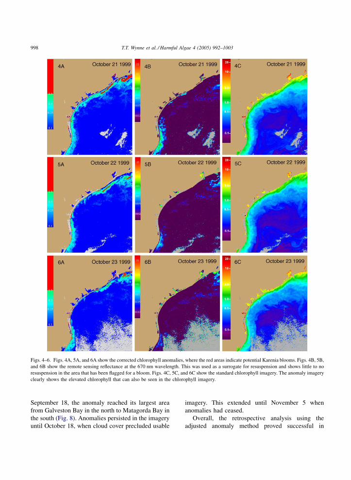
verified by field data. The imagery from October 21 to

23 show an anomaly on the northern coast of Texas,

and a smaller anomaly in the southern coast that may

be indicative of a much larger bloom than was

documented (see Figs. 4–6). There was a fish kill

reported to the TPWD in late October 1999 in the area

surrounding Brazos Santiago Pass (Villareal et al.,

2000). In addition, all the coastal sampling was within

the 9 nautical mile (15 km) state territorial waters. The

anomalies noted in Figs. 4–6 appeared to be further

offshore, and would not have been detected by the

field sampling.

3.2. 2000 HAB event

As was previously mentioned there was one large

and persistent bloom reported off Texas during our

study period, starting in August, 2000 and persisting

until November, 2000. This section will discuss how

well retrospective analysis did in documenting the

bloom during this period. On August 11, the first

report of a possible red tide was made when local

fisherman noticed thousands of black drum south–

southeast of Sabine Pass (northeastern coast of Texas)

by the Louisiana border. The TPWD investigated and

on August 14 discolored water in the region was

observed during an over flight. The discolored water

was positively identified as K. brevis. During this time

of the year, general circulation along the Texas coast is

from north to south (Cochrane and Kelly, 1986). This

alongshore circulation pattern transported K. brevis

cells southward down the coast. K. breviswas reported

in Galveston Bay on August 31, Matagorda Bay by

September 18, and Corpus Christi Bay on September

22. By October 3, the bloom had reached San Antonio

Bay. The bloom persisted in localized regions, such as

back bays and estuaries along the coast, until

November 8, when there were no longer positive cell

counts reported. The blooms were tracked through

bimonthly in situ sampling (Villareal and Magana,

2001).

Corrected anomaly images and cell counts were

examined for this period of time. By August 31, a

small anomaly developed south of Galveston Bay. On

September 3, 3 days after, the first positive cell counts

were recorded in the same general area (Fig. 7). By

September 12, a large anomaly had developed from

Galveston Bay to Matagorda Bay. This was the first

point that cell counts above 50,000 cells L�1 were

recorded. 50,000 cells L�1 is the limit of satellites to

detect K. brevis blooms (Tester et al., 1998). By


Figs. 4–6. Figs. 4A, 5A, and 6A show the corrected chlorophyll anomalies, where the red areas indicate potential Karenia blooms. Figs. 4B, 5B,

and 6B show the remote sensing reflectance at the 670 nm wavelength. This was used as a surrogate for resuspension and shows little to no

resuspension in the area that has been flagged for a bloom. Figs. 4C, 5C, and 6C show the standard chlorophyll imagery. The anomaly imagery

clearly shows the elevated chlorophyll that can also be seen in the chlorophyll imagery.

September 18, the anomaly reached its largest area

from Galveston Bay in the north to Matagorda Bay in

the south (Fig. 8). Anomalies persisted in the imagery

until October 18, when cloud cover precluded usable

imagery. This extended until November 5 when

anomalies had ceased.

Overall, the retrospective analysis using the

adjusted anomaly method proved successful in


Figs. 7–9. These images were taken during the Karenia bloom of 2000. Fig. 7A shows the standard chlorophyll anomaly. The boxes indicate the

position of positive cell counts. There is a small anomaly located in the vicinity of Bolivar Roads Pass. Fig. 7B shows the 670 reflectance

anomaly, used as a surrogate for suspended sediment concentrations. Fig. 7C shows the corrected chlorophyll anomaly; note that all anomalies in

the original anomaly image are still visible. Fig. 8A shows the standard chlorophyll anomaly the ‘‘�’’ indicates samples with a cell count of 0.

The corrected chlorophyll anomaly keeps the anomaly where it was positively identified (Bolivar Roads Pass to Cavalle Pass) but the anomaly

disappears south of Cavalle Pass. There were no cell counts available to verify this. Fig. 9A shows the further spread of the bloom. There were no

cell counts available south of Baffin Bay to confirm or deny the anomaly present in the area.

monitoring the entire coastline for the spread of the

bloom. Most of the in situ cell counts were taken in the

back bays and estuaries of the Texas coastline, where

the majority of the state’s shellfish beds are located.

The remote sensing anomaly techniques are not

efficient in these types of estuarine environments, as


Figs. 10–12. Fig. 10 imagery taken just prior to the pass of Tropical Storm Beryl. Resuspension (10B) is very low and no chlorophyll anomaly is

present in either the uncorrected (10A) or corrected imagery (10C). Fig. 11A–C was from the day following the pass of the storm. Resuspension

(11B) is elevated, causing anomalies in the uncorrected image (11A), but these anomalies are removed by the correction (11C). Fig. 12A–C

shows a return to ‘‘normal’’ conditions, with low resuspension and no anomalies present.

we are limited by the 1 km field of view of the

SeaWiFS sensor.

The adjusted chlorophyll method did not take away

any of the confirmed anomalies. In some cases the

extent of the anomaly was reduced in the southern part

of the region. K. brevis was not reported south of

Baffin Bay. The region was initially flagged in several

images during the period of the bloom. After the

region was corrected for resuspension these anomalies

were removed in most cases until mid-October. Fig. 9


Fig. 13. Image 13A shows the original chlorophyll anomaly from September 26, 2002, with red areas indicating potential blooms. Fig. 13B

shows the 670 reflectance anomaly, which indicates very high rates of resuspension, which is misinterpreted as chlorophyll (13D). After

resuspension is accounted for the anomalies disappear (13C). Fig. 13E shows the wind distribution from Port Aransas, TX. Awind of only 7 m/s

was responsible for generating the large anomaly illustrated in 13A, demonstrating the critical need to correct for resuspension.


illustrates such a case. The anomaly traveled from the

south down the coast. There were no cell counts above

the threshold of 50,000 cells L�1 available to confirm

or deny this potential bloom at the time. It should be

noted that the area south of Baffin Bay to Brownsville

is sparsely populated and little field data was available

for the region, making it impossible to say whether the

method was effective in this portion of the coast.

3.3. Tropical Storm Beryl example

A time series of a resuspension event is illustrated in

Figs. 10–12. The image in Fig. 10 shows normal

conditions just before the pass of Tropical StormBeryl.

T.S. Beryl made landfall about 30 miles south of the

Texas–Mexico border the night of August 15, 2000,

with sustained winds of approximately 50 knots. This

would classify as a strong resuspension event. On

August 15 there were typical conditions, without

elevated chlorophyll concentrations, and relatively low

resuspension. On August 18 there was a high

concentration of resuspended materials that were

introduced into the water column, as illustrated in the

670 reflectance anomaly (Fig. 11B). Note the presence

of an anomaly that developed in the image in Fig. 11A

before the correction, and the removal of the anomaly

after the correction as seen in Fig. 11C, which produces

results consistent with the phytoplankton chlorophyll

anomaly found in Fig. 10A. By August 20 conditions

returned back to normal, with low resuspension rates

and no chlorophyll anomalies (Fig. 12). The August 20

image also indicates that the resuspension did not cause

development of a new plankton algal bloom.

3.4. Additional resuspension event

There aremany smaller resuspension events inTexas

that are not due to major events like tropical storms. A

shift in wind direction can be enough of a forcing

function to cause a resuspension event. An example of

one such resuspension event is illustrated in Fig. 13.

Fig. 13A shows the chlorophyll anomaly from

September 26, 2002 before the image was corrected

for resuspension. Fig. 13B shows the 670 reflectance

anomaly. Fig. 13C shows the chlorophyll anomaly after

the image has been adjusted for resuspension. There

were extensive anomaly areas offshore before the

adjustment, and the anomalies were totally removed

after the image was corrected for resuspension. These

anomalies are implied when observing the standard

chlorophyll concentration, as seen in Fig. 13D. This

example illustrates that the forcing function behind a

resuspension event does not need to be as dramatic as a

tropical storm or a hurricane. Fig. 13E shows the graph

of wind data from a National Oceanic and Atmospheric

Administration (NOAA) Coastal-Marine Automated

Network (C-MAN) buoy located at Port Aransas, TX.

The graph is for the entire month of September. On

September 24 (Julian Day 267), 2 days before the date

of the image, the winds began blowing from the north

towards the south with a speed of approximately 7 m/s.

While this is slightly above themeanwind speed for this

area it is by nomeans ameteorological anomaly and is a

fairly regular occurrence. It is important to note that not

every 670 reflectance anomaly is as a direct result of

resuspension. River plumes can cause reflectance

anomalies, but rivers in Texas are relatively small

and will produce localized anomalies in the 670. It is

possible that some blue-green algae blooms can

produce 670 anomalies. 670 reflectance anomalies that

occur along large portions of the coast are for the most

part as a direct result of resuspension.

4. Conclusions

Overall the adjusted chlorophyll method proved

successful. Known blooms were identified in imagery

during the 2000 bloom. Unconfirmed anomalies were

eliminated by over 40% during non-bloom periods.

Unconfirmed anomalies that remained after the

correction can be attributed to a number of possibi-

lities. The Texas coast has a higher background

chlorophyll concentration than Florida does in non-

bloom conditions, implying that the region is a more

productive area than is Florida (Muller-Karger et al.,

1991). Therefore a strong possibility exists that many

of these remaining anomalies could be from other

phytoplankton, such as a bloom of non-toxic diatoms.

This monitoring method does not work reliably east of

Galveston Bay, as the Mississippi River plume

dominates the optical properties of this water and

anomalies must be viewed with a high degree of

skepticism. The method worked well for the remain-

ing portion of the Texas coastline, from Galveston Bay

to off shore of Laguna Madre.


Adjusting the chlorophyll anomaly for resuspen-

sion produces reasonable and consistent HAB detec-

tion for this coast. It may also provide improvements

in HAB detection along the Florida coast as well. The

method also provides insights into the blooms that are

exclusively planktonic.

Ideally the western Gulf of Mexico will be

incorporated into a satellite HAB monitoring system.

Stumpf et al. (2003) describes in detail a system

deployed by NOAA to monitor HABs in the gulf using

anomaly methods as were described in this paper. In

the future the same monitoring system will be

incorporated to the Texas coast.

References

Baden, D.G., Fleming, L.E., Bean, J.A., 1995. Chapter: marine

toxins. In: deWold, F.A. (Ed.),Handbook of Clinical Neurology:

Intoxications of the Nervous System. Part H. Natural Toxins and

Drugs. Elsevier Press, Amsterdam, pp. 141–175.

Cahoon, L.B., Redman, R.S., Tronzo, C.R., 1990. Benthic micro-

algal biomass in sediments of Onslow Bay, North Carolina.

Estuar. Coast. Shelf Sci. 31, 805–816.

Cahoon, L.B., Laws, R.A., 1993. Benthic diatoms from the North

Carolina continental shelf: inner and mid shelf. J. Phycol. 29,

257–263.

Cochrane, J.D., Kelly, F.J., 1986. Low-frequency circulation on the

Texas-Louisiana continental shelf. J. Geophys. Res. 91 (C9)

10,645–10,659.

Goddard, L., Mason, S.J., Zebiak, S.E., Ropelewski, C.F., Basher,

R., Cane, M.A., 2001. Current approaches to seasonal-to-inter-

annual climate predictions. Int. J. Climatol. 21, 1111–1152.

Haddad, K.D., 1982. Hydrographic factors associated with west

Florida toxic red tide blooms: an assessment for satellite pre-

diction and monitoring. M.Sc. Thesis. University of South

Florida, St. Petersburg, FL.

Kusek, K.M., Vargo, G., Steidinger, K., 1999. Gymnodinium breve

in the field, in the lab, and in the newspaper – a scientific and

journalistic analysis of Florida red tides. Contrib. Mar. Sci. 34,

1–228.

Magana, H.A., Contreras, C., Villareal, T.A., 2003. A historical

assessment of Karenia brevis in the western Gulf of Mexico.

Harmful Algae 2, 163–171.

Manheim, F.T., Hathaway, J.C., Uchupi, E., 1972. Suspended matter

in the surface waters of the northern Gulf of Mexico. Limnol.

Oceanogr. 17 (1), 17–27.

Muller, J.L., 1979. Prospects for measuring phytoplankton bloom

extent and patchiness using remotely sensed ocean color image:

an example. In: Toxic Dinoflagellate Bloom, Elsevier, North

Holland, Inc., New York, pp. 303–308.

Muller-Karger, F.E., Walsh, J.J., Evans, R.H., Meyers, M.B., 1991.

On the seasonal phytoplankton concentration and sea surface

temperature cycles of the Gulf of Mexico as determined by

satellites. J. Geophys. Res. 96 (C7) 12,645–12,665.

Nelson, J.R., Eckman, J.E., Robertson, C.Y., Marinelli, R.L., Jahnke,

R.A., 1999. Benthic microalgal biomass and irradiance at the sea

floor on the continental shelf of the South Atlantic Bight: spatial

and temporal variability and storm effects. Continental Shelf

Res. 19, 477–505.

Radziejewska, T., Fleeger, J.W., Rabalais, N.N., Carman, K.R.,

1996. Meiofauna and sediment chloroplastic pigments on the

continental shelf off Louisiana, USA. Continental Shelf Res. 16

(13), 1699–1723.

Stumpf, R.P., Arnone, R.A., Gould, R.W., Martinolich, P., Ransi-

brahmanakul, V., Tester, P.A., Steward, R.G., Subramaniam, A.,

Culver, M., Pennock, J.R., 2000. SeaWiFS ocean color data for

US Southeast coastal waters. In: Proceedings of the Sixth

International Conference on Remote Sensing for Marine and

Coastal Environments, Charleston, SC, Veridian ERIM Intl. Ann

Arbor, MI, USA, pp. 25–27.

Stumpf, R.P., Culver, M.E., Tester, P.A., Tomlinson, M., Kirkpa-

trick, G.J., Pederson, B.A., Truby, E., Ransibrahmanakul, V.,

Soracco, M., 2003. Monitoring Karenia brevis blooms in the

Gulf of Mexico using satellite ocean color imagery and other

data. Harmful Algae 2, 147–160.

Stumpf, R.P., Pennock, J.R., 1989. Calibration of a general optical

equation for remote sensing of suspended sediments in a mod-

erately turbid estuary. J. Geophys. Res. 94 (C10), 14363–14371.

Tester, P.A., Stumpf, R.P., Steidinger, K., 1998. Ocean color ima-

gery: what is the minimum detection level for Gymnodinium

breve blooms? Xunta de Galicia and Intergovernmental Ocea-

nographic Commission of UNESCO.

Tomlinson, M.C., Stumpf, R.P., Ransibrahmanakul, V., Truby, E.W.,

Kirkpatrick, G.J., Pederson, B.A., Vargo, G.A., Heil, C.A., 2004.

Evaluation of the use of SeaWiFS imagery for detecting Karenia

brevis harmful algal blooms in the eastern Gulf of Mexico. Rem.

Sens. Environ. 91 (3–4), 293–303.

Villareal, T.A., Brainard, M.A., McEachron, L.W., 2000. Gymno-

dinium breve (Dinophyceae) in the western Gulf of Mexico:

resident versus advected populations as a seed stock for blooms.

Harmful Algae Blooms. Intergovernmental Oceanographic

Commission of UNESCO 2001.

Villareal, T.A., Magana, H.A., 2001. A red tide monitoring program

for Texas coastal waters. Final Report. Texas Parks and Wildlife

Department. Contract 66621. UTMSI Technical Report TR04-

002.

detecting karenia brevis blooms and algal resuspension in the

Documents