detecting geomorphic responses following invasive vegetation
TRANSCRIPT

Detecting geomorphic responses following invasive vegetation removal: Wickaninnish
Dunes, Pacific Rim National Park Reserve, British Columbia, Canada
by
Jordan Blair Reglin Eamer
B.Sc., University of Victoria, 2010
A Thesis Submitted in Partial Fulfillment of the
Requirements for the Degree of
MASTER OF SCIENCE
In the Department of Geography
© Jordan Blair Reglin Eamer, 2012
University of Victoria
All rights reserved. This thesis may not be reproduced in whole or in part, by
photocopying of other means, without the permission of the author.

ii
Detecting geomorphic responses following invasive vegetation removal: Wickaninnish
Dunes, Pacific Rim National Park Reserve, British Columbia, Canada
by
Jordan Blair Reglin Eamer
B.Sc., University of Victoria, 2010
Supervisory Committee
Dr. Ian J. Walker, Department of Geography
Supervisor
Dr. K.O. Niemann, Department of Geography
Departmental Member

iii
Supervisory Committee
Dr. Ian J. Walker, Department of Geography
Supervisor
Dr. K.O. Niemann, Department of Geography
Departmental Member
Abstract
This thesis presents results from a large-scale dynamic restoration program
implemented by Parks Canada Agency (PCA) to remove invasive marram grasses
(Ammophila spp.) from a foredune-transgressive dune complex in Pacific Rim National
Park, British Columbia, Canada. The program goal is to restore habitat for endangered
Pink sandverbena (Abronia umbellate var breviflora) as required by the Canadian
Species at Risk Act (SARA). Three sites were restored by PCA via mechanical removal
of invasive marram grasses (Ammophila spp.) in September 2009. This study documents
geomorphic and sediment mass exchange responses at one of these sites as derived from
detailed Digital Elevation Model (DEM) surveys of a 10 320 m2 study area that spans
three discrete geomorphic units (beach, foredune, and transgressive dune complex).
Subsequent approximately bi-monthly total station surveys for the first year post-
restoration are compared to a pre-restoration baseline Light Detection and Ranging
(LiDAR) survey (August 2009) to quantify and describe morphodynamic responses and
volumetric changes. Two different methodologies were utilized for post processing of
volumetric change DEMs in order to filter out non-statistically significant change. The
first filter used software developed for fluvial geomorphology and was tested using the
student’s t distribution. This approach, while novel in the field of coastal geomorphology,
was less complex than the second which was based on spatial statistical procedures

iv
popular in the ecological sciences. This filter was based on local Moran’s Ii, which was
used to generate 1.5m and 5m distance thresholds of statistically significant geomorphic
change. These thresholds were specified to simulate the outer limit of saltating grains and
the dimensions of landform development, respectively. Results show that the beach
receives appreciable sediment supply via bar welding and berm development in the
winter, much of which is transported to the foredune and transgressive dune complex
units in the spring. This promotes rapid redevelopment of incipient dunes in the
backshore, rebuilding of the seaward slope of the foredune following wave scarping, and
localized extension of depositional lobes in the transgressive dune complex fed by
sediment from the beach and foredune stoss (only shown in local Moran’s Ii results). The
results of this study suggest that the foredune-transgressive dune complex at
Wickaninnish Dunes has experienced enhanced aeolian activity and positive sediment
volume changes over the first year following mechanical restoration. In addition,
comparison of the two methodologies show that spatial statistics were found to provide
both more realistic calculated volumes at a smaller threshold distance (e.g., – 0.012m3 m
-
2 in the foredune after devegetation; only +0.015m
3 m
-2 in the transgressive dune complex
in the year following restoration) and better highlighting of important spatial processes at
a larger threshold distance (e.g., foredune stoss erosion; feature highlighting) than the
volumetric change calculations based on a simpler statistical threshold.

v
Contents
Supervisory Committee ...................................................................................................... ii
Abstract .............................................................................................................................. iii
Contents ...............................................................................................................................v
List of Figures .................................................................................................................... ix
List of Tables ................................................................................................................... xiv
Acknowledgements ............................................................................................................xv
1. Introduction ......................................................................................................................1
1.1. Research Context .................................................................................................1
1.1.1. Coastal dune morphodynamics ...............................................................1
1.1.2. Technological advances in characterizing coastal dunes ........................3
1.1.3. Coastal dune restoration ..........................................................................6
1.1.4. Research gap ...........................................................................................9
1.2. Thesis structure and research purpose and objectives .......................................10
2. Geomorphic and sediment volume responses of a coastal dune complex to invasive
vegetation removal: Wickaninnish Dunes, Pacific Rim National Park Reserve, British
Columbia, Canada .........................................................................................................12
2.1. Abstract..............................................................................................................12
2.2. Introduction .......................................................................................................13
2.2.1. Research Purpose and Objectives .........................................................16

vi
2.3. Regional Setting ................................................................................................17
2.3.1. Study area and environmental setting ...................................................17
2.3.2. Study site location and rationale ...........................................................20
2.4. Methods .............................................................................................................22
2.4.1. Data collection ......................................................................................23
2.4.2. Data pre-processing...............................................................................28
2.4.3. Geostatistical modeling .........................................................................30
2.4.4. DEM generation and cross-shore topographic profile extraction .........32
2.2.5. Volumetric calculations and geomorphic change map generation .......33
2.5. Results ...............................................................................................................34
2.5.1. Cross shore topographic profile changes ..............................................34
2.5.2. Geomorphic and sediment volumetric change responses .....................36
2.6. Discussion..........................................................................................................41
2.6.1. Methodological implications.................................................................41
2.6.2. Volumetric and geomorphic responses of the beach-dune system to
vegetation removal ................................................................................42
2.6.3. Ascribing observed responses to the impacts of dune restoration ........47
2.6.4. Effectiveness of mechanical restoration for enhancing foredune
morphodynamics ...................................................................................51
2.7. Conclusions .......................................................................................................54

vii
2.8. Acknowledgements ...........................................................................................56
3. Quantifying spatial and temporal trends in beach-dune volumetric changes using
spatial statistics ..............................................................................................................57
3.1 Abstract...............................................................................................................57
3.2. Introduction .......................................................................................................58
3.2.1. Context and research objectives ............................................................58
3.2.2. Regional Setting ....................................................................................62
3.3. Methods .............................................................................................................65
3.3.1. Data collection and DEM generation ....................................................65
3.3.2. Application of local Moran’s Ii .............................................................66
3.4. Results ...............................................................................................................67
3.4.1. Moran’s I statistics and mapped clusters of deposition and erosion .....68
3.4.2. Geomorphic and sediment volume changes ..........................................72
3.5. Discussion..........................................................................................................77
3.5.1. Interpretation of local Moran’s Ii results and their geomorphic
relevance ................................................................................................77
3.5.2. Geomorphic responses within the beach-dune system .........................81
3.5.3. Comparison of local Moran’s Ii generated geomorphic change
thresholds and those using GCD ...........................................................86
3.6. Conclusions .......................................................................................................89

viii
3.7. Acknowledgements ...........................................................................................90
4. Conclusion .....................................................................................................................92
4.1. Summary and conclusions .................................................................................92
4.2. Research contributions and future directions ....................................................94
5. References ......................................................................................................................96

ix
List of Figures
Figure 1. Study area showing the nearby town of Ucluelet and the climate station from
which meteorological data were derived in Beaugrand (2010). Inset contains the
annual wind rose for the study region. Data are from the Environment Canada
climate station Tofino A [EC-ID 1038205] for the period 1971 to 1977 (from
Beaugrand, 2010). ................................................................................................. 19
Figure 2. Map of study site with monitoring profiles from Walker and Beaugrand (2008),
beach-dune complex under investigation, and foredune restoration coverage. .... 21
Figure 3. Survey points collected using the laser total station. Point patterns show the
systematic nested technique, where surveyors follow a grid pattern, deviating to
allow more coverage of areas with more topographic relief (continued on the
following page). .................................................................................................... 25
Figure 4. (cont’d) Survey points collected using the laser total station. Point patterns
show the systematic nested technique, where surveyors follow a grid pattern,
deviating to allow more coverage of areas with more topographic relief. ............ 26
Figure 5. Transport potential and relative transport potentials for the study area (from
Beaugrand, 2010) for specific months represented by DEM in Figure 6. Roses
indicate the strongly bimodal annual transport regime (right) with transport from
the WNW prevailing in summer and from the SE prevailing in winter (left). Axes
represent azimuth (angle) and transport potential (magnitude) in m3m
-1month
-1. 27
Figure 6. Map of the study area separated into discrete geomorphic units: beach, foredune
and transgressive dune complex. The outer boundaries were defined by the outer
limits of the survey with the smallest areal coverage. The inner boundaries

x
(essentially bounding the shoreward and landward limits) of the foredune are
defined in section 3.2. The dashed line gives the location of the extracted
topographic profiles shown in Figure 6, chosen as a subset of the full profile
(from landward boundary of the transgressive dune to lower beach) to highlight
changes important to the restoration effort (the upper beach, foredune, and
foredune lee). Bracketed letters show locations from which photos were taken for
Figure 9 (a-e)......................................................................................................... 29
Figure 7. Topographic cross-shore profiles extracted from interpolated DEM data. Survey
dates selected are those used in the geomorphic change maps in Figure 7. ......... 35
Figure 8. Geomorphic change maps of the study area selected to show beach and dune
trends. Survey date and Julian day in brackets are shown above each map. ........ 38
Figure 9. Area-normalized volumetric results determined to be statistically significant
based on GCD methodology described above. ..................................................... 44
Figure 10. (a,b) Vantage photos of the foredune from March and July. Note the scarping
and rebuilding of the foredune ramp, and accretion in the incipient dune zone in
the upper beach with associated seasonal vegetation. (c,d) Vantage photos of the
lee-side of the foredune for December and April. Deposition lobe is developing,
killing off of perennial vegetation, and liberating dune sediment in the area for
transport further into the transgressive dune. (e) Transgression on the eastern edge
of the transgressive dune complex. See Figure 5 for photo locations. ................. 46
Figure 11. Topographic profiles modified from Darke and Walker (2010) for the study
site, showing a year of change prior to and a year following restoration. Note that
xi
issues with the chart datum definition don’t allow for direct overlay on Fig. 6,
however form and relative change agree with data gathered for this study. ......... 49
Figure 12. Annual geomorphic change map of an area roughly 600m to the NW from the
study site, modified from Darke et al. (in review). Dashed line represents the
extent of vegetation removal undertaken in September, 2009 (note the landward
extent). Solid line represents geomorphic unit delineations (as in Figure 5). Note
the absence of large, developed depositional lobes in the lee of the foredune (i.e.,
up against the landward extent of the foredune unit). This image is provided for
comparison to the “Annual total” geomorphic change map from Figure 7. ......... 51
Figure 13. Map of the study area separated into discrete geomorphic units: beach,
foredune and transgressive dune complex. The outer boundaries were defined by
the outer limits of the survey with the smallest areal coverage. The inner
boundaries (essentially bounding the shoreward and landward limits) of the
foredune are defined in Section 2. ........................................................................ 65
Figure 14. Select maps of local Moran’s Ii -generated clusters of significant surface
change for the study site. Survey date shown in the upper right corner of each
map. These maps were generated using a 1.5m TD spatial weight. ..................... 70
Figure 15. Select maps of local Moran’s Ii -generated clusters of significant surface
change for the study site. Survey date shown in the upper right corner of each
map. These maps were generated using a 5m TD spatial weight. ........................ 71
Figure 16. Select geomorphic change maps of the study area, with the survey date shown
in the upper right corner of each map. These maps generated after applying the
1.5m TD local Moran’s Ii statistics as a significant change threshold. ................. 74

xii
Figure 17. Select geomorphic change maps of the study area, with the survey date shown
in the upper right corner of each map. These maps generated after applying the
5m TD local Moran’s Ii statistics as a significant change threshold. Circles on the
annual (August) change map indicate areas of interest discussed in section 3.5.3.
............................................................................................................................... 75
Figure 18. Picture taken in August 2010 of the back of the transgressive dune complex,
showing the deflation area upwind of the precipitation ridge, with two yellow
sand verbena plants in the foreground. Note the localized deposition around each
plant....................................................................................................................... 80
Figure 19. Picture taken in August 2010 of a blowout in the transgressive dune complex
with the trailing rhizomes of a big-head sedge plant located behind the researcher.
Note the linear localized accretion surrounding the vegetation-anchored sediment
(similar to the trailing arm of a parabolic dune). .................................................. 81
Figure 20. Volumetric change time series in the dune system after the initial LiDAR
survey for each geomorphic unit. Note the values from the two TD spatial weights
generated in this study and the values from the GCD analysis approach from
Section 2................................................................................................................ 82
Figure 21. Sand sheet creating a transport pathway through the foredune at the study site.
Photo taken August 2010. Location highlighted as the NW-most yellow circle in
Fig. 16 ................................................................................................................... 84
Figure 22. Photo at the study site showing: i) deflation at the foredune toe in front of the
tree island, visible by the coarser, darker sediment located in the depression, and
ii) accretion in the upwind (i.e., left) side of the tree island, visible by the Sitka

xiii
Spruce die-off due to burial. Photo taken August 2010 with the location indicated
by the SE-most yellow circle in Fig. 16. ............................................................... 85

xiv
List of Tables
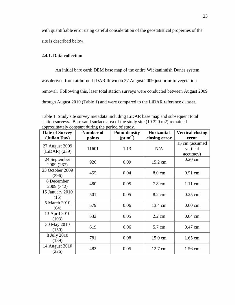
Table 1. Study site survey metadata including LiDAR base map and subsequent total
station surveys. Bare sand surface area of the study site (10 320 m2) remained
approximately constant during the period of study............................................... 23
Table 2. Results of cross-validation for this study, showing mean cross-validation (c-v)
error, standard deviation of the cross- -v) across all sampled
locations, and combined error (mean + 95% confidence interval + instrument
precision)............................................................................................................... 31
Table 3. Estimates of statistically significant sediment volume changes determined using
the GCD methodology (Wheaton et al. 2010). Area-normalized values (m3 m-2)
provide an effective depth of average sediment accretion (+) or erosion (-) within
each unit. ............................................................................................................... 39
Table 4. Global Moran’s statistics for each change DEM dataset indicate the presence of
global spatial autocorrelation. ............................................................................... 68
Table 5. Areal coverage of each result of local Moran’s Ii analyses, where Dh is
deposition hotspot, Do is deposition outlier, Eo is erosion outlier, and Ec is
erosion coldspot. ................................................................................................... 69
Table 6. Estimates of statistically significant sediment volume changes using spatial
statistical thresholds. Area normalized values (in brackets) provide an effective
depth of average sediment accretion (+) or erosion (-) within each unit. ............. 73

xv
Acknowledgements
A big thank you to my supervisor, Ian Walker, for his guidance and motivation
through these last two years. Thank you to my committee member, Olaf Niemann for
opportunities in his lab and general LiDAR prowess.
To my labmates, past and present, thanks for keeping me sane! You know who
you are HERB, DK, (Dr.) Darke, CC, KA, NvW.
To my brother, mom, and dad, thanks for believing!
To my partner JL, thanks so, so much for your support.
To my little boy, Tyler…
let's go on vacation!

1. Introduction
1.1. Research Context
1.1.1. Coastal dune morphodynamics
Aeolian (windblown) sediment transport is a key component to coastal
geomorphology, and associated dune formation is a function of the volume of available
sand on the beach, the shape and width of the beach, and the nature of the wind regime
(i.e., frequency, magnitude and directionality) (Short and Hesp, 1982; Psuty, 2004).
Vegetation and other roughness elements (e.g., large woody debris) in the backshore trap
sand allowing for the formation and growth of foredunes (Hesp, 2002; Eamer and
Walker, 2010). Beach-dune dynamics are a key factor in the classification of beaches
(Short and Hesp, 1982). Incoming wave energy (high, moderate, low) is directly related
to beach form (dissipative, intermediate, reflective) and geomorphology landward (large-
scale transgressive dune complexes and large stable foredunes, isolated parabolic dunes
and blowouts with moderate and unstable foredunes, minimal landward aeolian
deposition with small foredunes). The wind regime ultimately controls beach-dune
dynamics, sediment transport beyond the backshore and develop established foredunes,
and the size of the dune (Short and Hesp, 1982), and greater onshore wind velocity
increases the potential for sediment transport to the backshore and foredunes. Sediment
availability is one of the dominating variables that drives the development of the
foredune characteristics, though it regularly depends on the transporting availability of
the waves (Hesp, 2002; Psuty, 2004). Additional factors controlling dune development
include: (i) sand supply; (ii) vegetation characteristics; (iii) rate of aeolian sand accretion

2
and/or erosion; (iv) charactertics of transporting winds; (v) the occurrence and magnitude
of storm erosion, dune scarping, and overwash processes; (vi) medium to long term beach
or barrier state; (vi) sea/lake/estuary water level; (vii) extent of human impact and use
(Hesp, 2002)
Improved understanding of coastal dune dynamics is important in light of ongoing
and future impacts of climate change and sea level rise. As eustatic sea level appears to
be rising in many areas at about 1-2 mm/y over the past century (Gornitz, 1995), coastal
scientists are tasked with providing reasonable scenarios for the effects of sea-level rise
on coastal processes and shoreline position (Davidson-Arnott, 2005). The de-facto
standard for half a century was the Bruun Model (Bruun, 1954), which is constructed
from three hypotheses resulting from an increase in sea-level (Bruun, 1962): i) wave
erosion erodes the upper beach, ii) the exact volume of material from the upper beach is
deposited in the nearshore, and iii) the thickness of nearshore deposition is equivalent to
the amount of sea-level rise. While this served the purposes of the time, understanding of
backshore dynamics and the relationship between beach and dune sediment budgets (e.g.,
Nickling and Davidson-Arnott, 1990; Psuty, 1988; Sherman and Bauer, 1993), along with
the complete disregard for coastal dune sediment budget inherent in the Bruun Model, led
to a conceptual re-evaluation by Davidson-Arnott (2005). In this model, termed the RDA
model, three key components are discussed: i) the beach and foredune are eroded as a
result of sea level rise, and the beach-dune interface migrates shore- and upward, ii)
nearshore migration of sediment keeps pace with rising sea level, and iii) all sediment
eroded from the dune is transferred landward, resulting in landward migration of the
foredune and no net loss of sediment from the dune. Better understanding of foredunes as

3
dynamic features in the event of sea-level change is warranted as they often act as
important buffers for shore-proximal ecosystems and coastal towns to coastal erosion,
storm surges, and gradual sea level rise.
Coastal dune systems are the manifestation of a suite of processes and
sedimentary responses that are difficult to model, ergo studies typically adopt one of
three perspectives: i) beginning at the micro scale, with the investigation of sediment
entrainment and boundary layer airflow; ii) beginning at the macro-scale, looking at a
beach-dune system or dunefield and reconstructing the environmental history of the
system; iii) the emerging approach of confining the study to the meso-scale, with data
collection spanning longer temporal scales and the increasing use of digital elevation
models (DEMs) to represent process-response dynamics. Despite advances in these three
areas, the field has suffered from difficulties in bridging the scales, as the three
approaches are conceptually and methodologically incompatible (Sherman, 1995).
1.1.2. Technological advances in characterizing coastal dunes
Given the broad spatial and temporal scales the field of geomorphology operates
in, advances in knowledge often correspond with advancements in methods of data
collection and management. The advent of airborne Light Detection and Ranging
(LIDAR) has opened up new insights into meso- and macro-scale surface dynamics.
Recent studies have used LIDAR in evaluating climate change impacts due to sea level
rise (e.g., Webster et al., 2006), monitoring beach nourishment (e.g., Gares et al., 2006),
and environmental reconstruction of a coastal system to assess response to sea-level
change (e.g., Wolfe et al., 2008). Brock et al. (2002) show how LIDAR can be used for

4
the regional mapping of geomorphic change along sandy coasts in the United States,
particularly in response to storms or long-term sedimentary processes such as coast
progradation. Sallenger et al. (2003) used airborne topographic LIDAR to quantify beach
topography and change along the North Carolina coast. Using LIDAR data to quantify
volumetric changes in coastal systems is gaining momentum (e.g., Woolard and Colby,
2002; Zhang et al., 2005), however issues with how this relatively new data-collection
method in the generation of DEMs must be taken into account (Liu, 2008). LIDAR is
also an extremely powerful tool when combined with other remote sensing techniques
such as with multi- or hyperspectral images for the classification of coastal land covers
(e.g., Lee and Shan, 2003) or studying beach morphodynamics (e.g., Debruyn et al.,
2006).
Interpolation, defined as reconstruction of the underlying continuous field of data
from the limited evidence of the control points (O'Sullivan and Unwin, 2003), is of
growing importance in the quantitative aspects of the natural sciences. It has existed for
decades, flourishing with the advent of Geographic Information Systems in the 1960's,
and traditionally has relied on deterministic methods such as proximity polygons, local
spatial average, nearest neighbour, inverse-distance weighted spatial average,
Triangulated Irregular Network (TIN), and spline fitting (O'Sullivan and Unwin, 2003).
Of these, only nearest neighbour (when the data density is sufficiently high, such as in
Light Detection and Ranging (LIDAR) datasets (Liu, 2008)) and spline fitting (e.g.,
Mitasova et al., 2005) are still commonly used in coastal analysis.
In a general sense, these surfaces can be approximated by letting the data speak
for itself by application of regression methods to spatial coordinates, termed trend surface

5
analysis (O'Sullivan and Unwin, 2003). The results from this analysis can be thought of
as a first-order trend in the data, as it is often a linear trend surface (plane). What
differentiates this method from those previously mentioned is that the surface is
generated as a best-fit to the data, is not an exact interpolator (doesn't honour all
datapoints), and as such outputs residuals from which the square of the coefficient off
multiple correlation (R2) can be calculated. Ergo this is the first interpolation method that
allows us to assess how well the model performed in interpolating the surface. Trend
surface analysis, however, is not without it's shortfalls: i) there is generally no reason to
assume that the attribute under analysis varies in such a simple way, ii) not all control
points are honoured, and iii) there is essentially no analyst input into the selection of the
trend surface model.
The decline in popularity of the aforementioned exact interpolator methods is
largely due to realization that there is a degree of arbitrariness in the choice of
interpolation algorithm parameters. For example, a typical approach with nearest
neighbour is to use trial and error to determine the number of neighbours to average—or
as with spline fitting, the smoothing and tension—with qualitative assessment of the
generated surface deemed sufficient to select one and reject another. The methodology,
while often “expert-driven”, does not refer to the characteristics of the data itself.
Conversely, trend surface analysis, while letting the data speak for itself, doesn't allow
for much (if any) “expert-driven” analysis, as it essentially regresses a surface to the data.
Ideally, there should be a interpolator that allows for both the characteristics of the data
and the knowledge that the analyst can offer. Krige (1951) devised a series of empirical
methods that would later become the basis for a suite of geostatistical interpolators
6
known as Kriging that was developed into a theoretical framework by Georges Matheron
(Agterberg, 2004). Kriging is considered an optimal (makes best use of what can be
inferred about the spatial structure of the surface) statistical (allows for the data to speak
for itself) interpolator (O'Sullivan and Unwin, 2003). In the simplest terms, it is the
combination of a distance-weighted method and trend surface analysis. It has only
recently been applied to the coastal sciences (e.g Swales, 2002; Woolard and Colby,
2002; Zhang et al., 2005). The basic principles of Kriging, and how they combine to
generate an optimal interpolator for coastal surfaces, is explained in Swales (2002).
While this study was confined to the beach setting, and did not extend past the backshore,
there were nevertheless valuable conclusions drawn, such as: i) de-trending the data via
trend surface analysis to satisfy the stationarity assumption (Goodman, 1983; Unwin,
1975) is an integral (and oft-forgotten) step, ii) experimental variograms display a high
degree of spatial continuity, and thus should be well approximated, whether by some
form of least-squares criteria, by trial and error (i.e., using cross-validation (Swales,
2002)), or from expert-driven approaches (Englund and Sparks, 1991), iii) short-term
changes in beach surface are more difficult to model significantly in periods of accretion
rather than periods of erosion, due to magnitude differences in the surface change, and iv)
an ideal methodology, rather than interpolating between profiles as was done by the
author, is to monitor a beach segment with an array of points.
1.1.3. Coastal dune restoration
Coastal and inland dunes have historically been subject to intense stabilization
efforts (e.g., Rozé and Lemauviel, 2004) to reduce wind erosion and sand drift (Grootjans
et al., 2002). Recently, more dynamic coastal restoration approaches that increase natural

7
geomorphic processes are utilized to provide more resilient landforms and, thus, more
favourable ecological conditions for native species (Nordstrom, 2008). As this is a recent
policy shift in only a few countries (the Netherlands (e.g., van Boxel et al., 1997; Arens
et al., 2004), New Zealand (Hilton, 2006), and the United States (e.g., Van Hook, 1985)
for example), there are few examples in the literature of documented dynamic coastal
restoration projects.
One example of a recent effort in restoring dynamism is provided by van Boxel et
al. (1997), for which several blowouts on the Dutch coast were re-activated and the
blowout morphology, vegetation dynamics, and lime content (i.e., Potential nutrients)
were monitored. Largely an ecological paper, the results from the three years of
monitoring indicated that:
1. The influence of relative humidity associated with weather systems on
morphological changes is great. For example, in the study site, although
easterly winds are less frequent and weaker than westerlies, morphology is
dominated by them due to the fact that they are associated with a low relative
humidity and precipitation,
2. The mosses in the study area tolerated little to no burial, whereas marram
grass was able to establish right in the blowout, and
3. Lime content was highest in the blowout, with diminished (but remaining)
lime in the depositional lobes. Marram grass and mosses contribute to soil
acidification.

8
Finally, the authors conclude that most of the small blowouts re-stabilized, whereas the
medium sized blowouts actually grew in area. The authors confirm that the marram grass
does not suffer from burial at all, actually requiring it for survival.
Arens et al. (2005) provides an account of a Dutch restoration of dune mobility at
three study sites. This paper shifts focus from documenting ecologic to geomorphic
response, using airphoto analysis for two of three sites (monitoring re-stabilization after
mechanical re-activiation) and summarizing results from Arens el al. (2004) for the third
site, which was much more extensively monitored using aerial photography, erosion pins,
and climate data analysis. Results showed a massive initial increase in aeolian activity,
with large vegetated areas invaded by sand and changing the vegetation dynamics of the
area. Deflation of the newly erodible sand led to a reduction in surface elevation, and
after five years significant portions of the dunes were re-stabilizing with vegetation,
outpacing naturally occurring newly activated areas. To achieve durable dune mobility,
the sand must remain active, whether by permanent or recurring disturbances or by the
presence of high-easily erodible dunes.
A more recent study in dynamic restoration was undertaken by Kollmann et al.
(2009). It involved mechanical removal of an invasive shrub from the coastal dunes of
Denmark. While some geomorphic information was taken in the vegetation mapping
process (i.e., identification of geomorphic unit, slope, and aspect), this study, similar to
the van Boxel et al. (1997) study, was concerned with documenting the ecological
response to restoration. Relative findings indicate that mechanical removal was not
sufficient for fully preventing re-sprouting of remaining vegetation fragments, and the
authors indicate that this is not unlike other results (e.g., D'Antonio and Meyerson, 2002).

9
Also, they recommend burial-enhancing structures (such as sand fences) over the restored
area to assist in preventing re-sprouts.
1.1.4. Research gap
The current state of coastal studies at the meso-scale is clearly lacking from at
least one of: proper characterization of the geostatistics involved in the study, an
appropriate interpolation method, an appropriate sampling method, a proper description
of error, and/or integration of that error into results to determine significant changes. To
date, a coastal study with properly reported geostatistics has not been documented using
the array of data recommended in Swales (2002). Nor has the realization that separation
into geomorphic units (beach, foredune, and transgressive dune complex) should
drastically decrease interpolation error, as they all exhibit drastically different underlying
trends due to the processes involved (swash dominated sediment transport, topographic
steering (Walker et al., 2006), and alignment to dominant wind direction (e.g., Arens,
2004; Martinho et al., 2010)) that are important to remove (Swales, 2002). Finally, proper
characterization of the geomorphic response of a coastal system to dynamic coastal
restoration hasn't been attempted, or reported in the literature, to date.
To reiterate Sherman (1995), the key to bridging the different scales of coastal
processes is at the meso-scale, and require proper characterization of surface change to be
correlated with process-based as well as environmental change assessment. Elaborating
upon that, Bauer and Sherman (1999) identify one of the two most pressing needs facing
the coastal aeolian sciences as the development of a robust conceptual framework or
grand, unifying theory that can serve as the template upon which we may inscribe our

10
contributions. Ten years later, Houser (2009) concedes that the development of a beach-
dune model that transcends scale barriers and field site restrictions still eludes coastal
scientists. While the stated goal of this research (defined below) is not to define such an
ambitious model, there is current demand for more properly, accurately undertaken
coastal meso-scale studies. The recent support for dynamic coastal restoration methods
will provide the laboratory.
1.2. Thesis structure and research purpose and objectives
This thesis is structured around two results sections (2 and 3) derived from data
collected between August of 2009 and 2010 at a beach-dune system located in the
Wickaninnish Dunes, Pacific Rim National Park Reserve, British Columbia, Canada.
These sections are bookended with an Introduction (Section 1) that sets the research
context and Summary and Conclusions (Section 4) that reviews key findings of the
research.
The general purpose of this research is to garner a better understanding of beach-
dune evolution through developing novel methodology for detecting surface change that
followed large-scale destabilization of the foredune. This purpose is explored through the
following research objectives. Section 2 examines ten topographic survey datasets
collected in a grid pattern over a beach, foredune, and transgressive dune complex (each
area termed separate geomorphic units) by determining statistically significant changes
between DEMs of each geomorphic unit, with significance evaluated using the student`s t
distribution. Specifically, the objectives of this paper are to: i) identify multi-temporal
and multi-spatial geomorphic changes between and over all geomorphic units at the study
site, ii) refine a methodology for identifying said change, and iii) assess the effectiveness

11
of the implemented treatment (dynamic dune restoration) for increasing dune activity.
This section has been submitted as a manuscript for peer review to the journal Earth
Surface Processes and Landforms, and is currently in revision (March, 2012).
Section 3 utilizes tools provided by the field of spatial statistics, namely local
Moran’s Ii, to assess statistically significant patterns and change at the study site using the
same dataset from Section 2. Specifically, the objectives of this paper are to: i)
investigate the applicability of local Moran’s Ii as applied to DEMs in a coastal setting, ii)
quantify and describe geomorphic change following foredune destabilization, and iii)
compare this method to a more conventional approach (Section 2). This section is a
revised draft of a manuscript for submission for peer review to the journal
Geomorphology.

12
2. Geomorphic and sediment volume responses of a coastal
dune complex to invasive vegetation removal: Wickaninnish
Dunes, Pacific Rim National Park Reserve, British Columbia,
Canada
2.1. Abstract
Recently, there has been a shift from restoring coastal dunes as stabilized
ecosystems to more dynamic systems that are geomorphically diverse, more resilient to
erosion, and that offer greater ecosystem diversity, particularly for pioneering (and often
endangered) species. This paper presents results from a large-scale dynamic restoration
program implemented by Parks Canada Agency (PCA) to remove invasive marram
grasses (Ammophila spp.) from a foredune-transgressive dune complex in Pacific Rim
National Park, British Columbia, Canada. The program goal is to restore habitat for
endangered Pink sandverbena (Abronia umbellate var breviflora) as required by the
Canadian Species at Risk Act (SARA). Three sites were restored by PCA via mechanical
removal of invasive marram grasses (Ammophila spp.) in September 2009. This study
documents geomorphic and sediment mass exchange responses at one of these sites as
derived from detailed DEM surveys of a 10 320 m2 study area that spans three discrete
geomorphic units (beach, foredune, and transgressive dune complex). Subsequent
approximately bi-monthly total station surveys for the first year post-restoration are
compared to a pre-restoration baseline LiDAR survey (August 2009) to quantify and
describe morphodynamic responses and volumetric changes. Results show that the beach
receives appreciable sediment supply via bar welding and berm development in the

13
winter (0.309 m3m
-2 between March and April) much of which is transported to the
foredune and transgressive dune complex units in the spring (annual values of 0.128 and
0.066 m3m
-2, respectively). This promotes rapid redevelopment of incipient dunes in the
backshore, rebuilding of the seaward slope of the foredune following wave scarping, and
localized extension of depositional lobes in the transgressive dune complex. The results
of this study suggest that the foredune-transgressive dune complex at Wickaninnish
Dunes has experienced enhanced aeolian activity and positive sediment volume changes
over the first year following mechanical restoration.
2.2. Introduction
Coastal dunes are geomorphically significant features that store and cycle large
amounts of sand. As such, they are key components of the coastal sediment budget (e.g.,
Short and Hesp, 1982; Hesp, 2002; Psuty, 2004) and they provide an important 'buffer'
along shorelines subject to extreme and/or increasing storm surge and erosion impacts
and more gradual sea-level rise (e.g., Davidson-Arnott, 2005; Houser et al., 2008;
Mascarenhas and Jayakumar, 2008; Eamer and Walker, 2010). Sand dunes are also
biological and ecologically significant (e.g., Grootjans et al., 2002; Hesp, 2002) as they
provide critical habitat for many specialized endemic, migratory and endangered species
(e.g., Wiedemann and Pickart, 1996) and as a natural resource and land use base (e.g.,
Nordstrom, 1990). In western Canada, less than 30% of the shoreline is partially sandy,
with less than 10% of this consisting of dune-backed sandy beaches. Thus, there is recent
interest in restoring coastal dunes from stabilized ecosystems with declining geomorphic
(aeolian) activity to more dynamic ecosystems with increased aeolian activity and

14
improved habitat for early successional (and often endangered) species (Nordstrom,
2008).
Recent work on coastal dune restoration (e.g., van Boxel et al. 1997, Nordstrom
2008, Kollmann et al. 2011) suggests that a more dynamic landscape, wherein
stimulation of natural geomorphic processes (e.g., aeolian activity) via vegetation
removal, provides a more resilient ecosystem with more favourable ecological conditions
for native and/or endangered species. This is a major shift from decades of restoration
for coastal dune stabilization, which has been practiced for a range of purposes from
forestry (e.g., Riksen et al., 2006) to wave erosion defense (e.g., Grootjans et al., 2002).
Recent efforts to restore for more dynamic coastal dune landscapes provide distinct
opportunities to quantify and examine sediment volume changes and transfer processes
and resulting morphodynamic responses that, in turn, provide useful information for
ecosystem management and coastal development (Nordstrom 2008).
Recent technological advancements have made for new developments in
understanding and modelling the micro- to meso-scale morphodynamics of coastal dune
systems, including: i) detailed airflow and sand transport experiments using high
resolution ultrasonic anemometry and high-frequency electronic sand transport devices
(e.g., Hesp et al., 2005; Walker et al., 2006; Lynch et al., 2008; Bauer et al., 2009;
Davidson-Arnott et al., 2009; Walker et al., 2009a; 2009b; Jackson et al., 2011; Chapman
et al., in review), ii) detailed mapping and quantification of beach-dune volumetric and
morphological changes using Light Detection and Ranging (LiDAR) (e.g., Woolard,
2002; Sallenger et al., 2003; Houser and Hamilton, 2005; Saye et al., 2005; Eamer and
Walker, 2010), iii) near-field remote sensing of sand transport events and morphological

15
responses (e.g., Darke et al., 2009; Delgado-Fernandez et al., 2009; Delgado-Fernandez
and Davidson-Arnott, 2011), and iii) computational simulation modelling of dune
dynamics (e.g., Baas, 2002; Baas and Sherman, 2006).
The dominant approach to analyzing beach-dune systems at the meso-scale is a
sediment budget approach, where sediment eroded from one component of the system is
accounted for by accretion in another component. Short and Hesp (1982), Psuty (1992),
Sherman and Bauer (1993), Arens (1997), and Hesp (2001) have each made efforts to
extend the approach to include various factors (e.g., nearshore inputs and morphology,
fetch effects, aeolian contributions to foredunes) that refine the scope and/or role of
inputs and outputs to the system. More recently, rapid, high resolution digital elevation
models (DEM) generated from terrestrial and subaqueous LiDAR have emerged for
characterizing volumetric and morphological responses, more in a mass-balance type
approach, in beach-dune systems (e.g., Woolard and Colby, 2002; Sallenger et al., 2003;
Houser and Hamilton, 2005; Saye et al., 2005; Eamer and Walker, 2010) and analytical
methods using open-source software for accurate analysis of change detection are
emerging (e.g., Wheaton et al., 2010).
The ability to use GIS and geostatistics to manipulate, visualize, and analyse
spatial patterns in geomorphic data has become increasingly important in coastal
research, especially at the meso-scale (Andrews et al., 2002). Various approaches have
been used to quantify and examine coastal sediment mass balance and landscape
responses using DEMs (e.g., Swales, 2002; Woolard and Colby, 2002, and Anthony et
al., 2006). However, the mass balance approach requires careful consideration of how
topographic and, thus, volumetric changes are defined and modelled so as to best

16
represent true changes within the system. Geostatistical interpolation methods (e.g.,
kriging) are often used to model the spatial continuity and trends in surface elevation data
from a field of spatially discontinuous point measurements so as to produce a spatially
representative DEM of a landscape at a given point in time. Spatial continuity models
(e.g., variograms) associated with these methods are also useful for quantifying and
potentially reducing errors associated with DEM generation from field data (Desmet,
1997). Spatial variograms have an experimental and model component. The
experimental variogram provides the best estimate for spatial variation in a variable (i.e.,
difference in some z value over distance) and the parameters (e.g., sill, range, nugget, see
Swales, 2002) are used to develop the best approximation model variogram. This model
variogram has mathematically uniform properties, thus enabling it to be used in DEM
generation (Swales, 2002).
2.2.1. Research Purpose and Objectives
The general purpose of this research is to accurately quantify and describe the
sediment volume and resulting geomorphic responses within a recently destabilized
foredune-transgressive dune system on the west coast of Vancouver Island, British
Columbia, Canada. In particular, the study applies statistical change detection methods
to high-resolution DEMs obtained from LiDAR and subsequent laser total station surveys
to estimate seasonal sand volume changes and describe resulting geomorphic responses.
As such, this research provides an initial assessment of the effects of mechanical
vegetation removal to promote more dynamic habitat. Specific research objectives are as
follows:

17
1. To quantify and describe significant seasonal volumetric and geomorphic
changes within linked beach, foredune, and transgressive dune landscape units
using detailed DEMs generated from recurrent site surveys for the first year
following mechanical removal of vegetation.
2. To refine a methodology developed for fluvial settings for optimal sampling
and processing of topographic survey data for accurate modelling and change
detection within a coastal dune system.
3. To interpret initial landscape responses to dune destabilization and assess the
effectiveness of the implemented treatment (complete vegetation removal) for
enhancing dune morphodynamics.
2.3. Regional Setting
2.3.1. Study area and environmental setting
The study area is the Wickaninnish Dunes complex within Pacific Rim National
Park Reserve (PRNPR), on Vancouver Island near Ucluelet, British Columbia, Canada
(Fig. 1). This area hosts 1 to 5 m high vegetated foredunes that are prograding at a rate of
approximately 0.2 m a-1
and are backed by the largest active transgressive dune complex
on Vancouver Island (Heathfield and Walker, 2011). The 10-km long embayed beach
has a mesotidal range (spring tide range ~4.2 m) and is exposed to energetic wave
conditions (average winter significant wave height of 2.47 m and period 12.07 s). Beach-
dune geomorphology varies slightly in Wickanninish Bay and the beach fronting the
Wickaninnish Dunes has a shoreline length of approximately 4.2 km and an uninterrupted
fetch to incoming winds and waves from the Pacific Ocean.

18
The climate in the study region is marine west coast cool (Cfb) per the Köppen
classification with an annual average air temperature of 12.8°C (1971-2000) and high
year-round precipitation (3305.9 mm). Rainfall occurs, on average, on 202.7 days of the
year with 52% falling from October through January and only 18% falling during the
summer months (May through August). Because of the mild temperatures and high
precipitation, the dunes at this site support a number of native plant species,
predominantly American dune (wildrye) grass (Leymus mollis), beach morning glory
(Convolvulus soldanella), beach carrot (Glehnia littoralis), and yellow sand verbena
(Abronia latifolia). Dominant species on the foredune, however, are the introduced
American and European beach (marram) grasses (Ammophila breviligulata and A.
arenaria, respectively). In the transgressive dunes, vegetation succession has lead to
encroachment by native Kinnikinnick (Arctostaphylos uva-ursi) and Sitka spruce (Picea
sitchensis).

19
Figure 1. Study area showing the nearby town of Ucluelet and the climate station from
which meteorological data were derived in Beaugrand (2010). Inset contains the annual
wind rose for the study region. Data are from the Environment Canada climate station
Tofino A [EC-ID 1038205] for the period 1971 to 1977 (from Beaugrand, 2010).
The introduced Ammophila is of special concern due to its aggressive expansion
on foredunes, reduction of dune biodiversity, and ability to significantly alter foredune
sediment budgets and morphodynamics (e.g., Wiedemann and Pickart, 1996; Hesp,
2002). At this site, Ammophila spp. have reduced habitat for the Grey beach pea vine

20
(Lathyrus littoralis), which is provincially red-listed as endangered, and the Pink
sandverbena (Abronia umbellate var breviflora), which is federally red-listed as
endangered under the Canadian Species at Risk Act (SARA). PRNPR is legally
obligated under SARA to develop a recovery strategy for Pink sandverbena and a 5-year
program of habitat restoration by Parks Canada Agency (PCA) is underway, which
provides the opportunity for this research. It is hypothesized that dense Ammophila
colonization of the foredune is responsible for reduced sand supply to, and resulting
stabilization of, the transgressive dunes at Wickaninnish, which experienced a decline of
28% in active sand surface area from 1973 to 2007 (Heathfield and Walker, 2011).
The west coast of Vancouver Island experiences frequent WNW summer winds
and strong SE winter storm winds (Eid et al., 1993; Beaugrand, 2010)(Fig. 1). The
geomorphology of the transgressive dune complex (e.g., alignment of erosional blowouts
and depositional lobes) suggests a dominant transport vector from the WNW driven by
(drier) summer wind events, despite a resultant sand transport potential vector from the
south (see Fig. 4, section 3.1). The combined effects of high precipitation during the
winter months (which increase sand transport threshold during typical SE storm winds),
local land and sea breezes, and topographic steering effects within the dunes and
vegetation stands, alter local sand transport pathways that have maintained the north-
westerly alignment of the transgressive dune complex.
2.3.2. Study site location and rationale
A stretch of approximately 3 km of foredune was identified by PCA in 2009 for
mechanical removal of Ammophila to restore dynamic dune habitat. The first phase of

21
removal occurred on 21 September 2009 with approximately 200 metres of foredune
cleared of vegetation on either side of four pre-existing, cross-shore coastal erosion
monitoring profiles (Walker and Beaugrand 2008) (Fig. 2). Profiles extend from the
beach over the foredune and transgressive dunes to the forest edge. At each site, invasive
plant cover was removed mechanically by a backhoe equipped with a specialized finger
bucket designed to reduce the amount of sand loss during the removal process.
Figure 2. Map of study site with monitoring profiles from Walker and Beaugrand (2008),
beach-dune complex under investigation, and foredune restoration coverage.

22
This study examines changes over the first year following vegetation removal at
the southeastern-most site (Fig. 2), which is a smaller transgressive dune complex fronted
by 75 m of fully denuded foredune and encompassed on all landward boundaries by
forest vegetation. The study site had 10 320 m2 of active sand surface and a perimeter of
924 metres, which remained essentially constant over the period of study. This site was
selected as it provided a spatially discrete entity for quantifying and describing significant
volumetric and morphological responses to the restoration treatment. The more northerly
sites in the larger transgressive dune complex have considerably more active sand
surface, much longer and open fetch distances, and, thus, appreciable lateral sand
transfers and aeolian bedform migration between sites. Thus, it is more difficult to
ascribe changes within these larger sites to the adjoined restoration treatment. However,
the incomplete devegetation of the most northerly site in Figure 2, a similar beach and
foredune morphology, and contemporaneous data collection at the site provided an ideal
control site for volumetric responses of a site not fully restored. Darke et al. (in review)
discuss the broader objectives and rationale for this restoration project and describe
responses at other locations within the broader dune complex.
2.4. Methods
To assess changes in site geomorphology and sediment volume transfers, repeat
(approximately bi-monthly) DEMs were produced using detailed topographic survey data
imported into a multitemporal GIS database from which change detection maps and
surface geostatistics were generated. The methodology for generating accurate DEMs
23
with quantifiable error using careful consideration of the geostatistical properties of the
site is described below.
2.4.1. Data collection
An initial bare earth DEM base map of the entire Wickaninnish Dunes system
was derived from airborne LiDAR flown on 27 August 2009 just prior to vegetation
removal. Following this, laser total station surveys were conducted between August 2009
through August 2010 (Table 1) and were compared to the LiDAR reference dataset.
Table 1. Study site survey metadata including LiDAR base map and subsequent total
station surveys. Bare sand surface area of the study site (10 320 m2) remained
approximately constant during the period of study.
Date of Survey
(Julian Day)
Number of
points
Point density
(pt m-2
)
Horizontal
closing error
Vertical closing
error
27 August 2009
(LiDAR) (239) 11601 1.13 N/A
15 cm (assumed
vertical
accuracy)
24 September
2009 (267) 926 0.09 15.2 cm
0.20 cm
23 October 2009
(296) 455 0.04 8.0 cm 0.51 cm
8 December
2009 (342) 480 0.05 7.8 cm 1.11 cm
15 January 2010
(15) 501 0.05 8.2 cm 0.25 cm
5 March 2010
(64) 579 0.06 13.4 cm 0.60 cm
13 April 2010
(103) 532 0.05 2.2 cm 0.04 cm
30 May 2010
(150) 619 0.06 5.7 cm 0.47 cm
8 July 2010
(189) 781 0.08 15.0 cm 1.65 cm
14 August 2010
(226) 483 0.05 12.7 cm 1.56 cm

24
Topographic survey data were collected using a Topcon GTS226 laser total
station. For every survey, the total station was re-sectioned (i.e., referenced) into a local
grid of control points that were established using a Real Time Kinematic (RTK) GPS
unit. As such, points were georeferenced on collection and required no post-processing.
The survey data collection strategy was a systematic nested pattern (Chappell et al.,
2003) (vs. a fixed positional grid of recurrently surveyed points) that captured detailed
coverage of significant features and slope inflection points with grid densities of 0.04 to
0.09 points m-2
and vertical accuracies (closing errors) of 0.04 to 1.65 cm (Table 1)
(Figure 3).
Beaugrand (2010) characterized the regional sand transport potential regime using
wind data from the Environment Canada meteorological station Tofino A (EC-ID
1038205) located at Tofino Airport (Fig. 1) that only recorded 24-hour observations from
1971 to 1977. Unfortunately, a meteorological station installed at the Wickaninnish
study site suffered instrument malfunctions during the first year of study and the dataset
was not continuous enough to be useful. Per Arens (2004), and using the six years of
Tofino Airport wind data, Beaugrand (2010) calculated annual and monthly sediment
transport potentials (Fig. 4). These data are used to provide first-order estimates of sand
transport potential conditions at the study site.

25
Figure 3. Survey points collected using the laser total station. Point patterns show the
systematic nested technique, where surveyors follow a grid pattern, deviating to allow
more coverage of areas with more topographic relief (continued on the following page).

26
Figure 4. (cont’d) Survey points collected using the laser total station. Point patterns
show the systematic nested technique, where surveyors follow a grid pattern, deviating to
allow more coverage of areas with more topographic relief.

27
Figure 5. Transport potential and relative transport potentials for the study area (from
Beaugrand, 2010) for specific months represented by DEM in Figure 6. Roses indicate
the strongly bimodal annual transport regime (right) with transport from the WNW
prevailing in summer and from the SE prevailing in winter (left). Axes represent azimuth
(angle) and transport potential (magnitude) in m3m
-1month
-1.

28
2.4.2. Data pre-processing
A digital orthophotograph mosaic was constructed for the study site using
imagery obtained during the LiDAR mission. Interpretation of the photo mosaic,
combined with field reconnaissance, was then used to delineate the study site into three
discrete geomorphic units: beach, foredune, and transgressive dune complex (Fig. 5).
This delineation made volumetric response comparisons within the same unit over time
possible. Also, due to the different formative processes of features within the beach,
foredune and transgressive dune units (i.e., swash zone dynamics, aeolian dominated
transport, etc.), unit separation also allowed for more representative geostatistical
modeling. This refines the interpolation method and provides some geomorphic
rationale, as kriging takes directionality and variation distance, or orientation and size of
features respectively, in to account. The beach unit was approximately 80 metres wide
and was defined on the seaward margin by the limits of the survey and on the landward
margin by the seaward extent of established foredune vegetation (e.g., Ammophila spp.
and/or Leymus mollis). As such, the beach unit included an ephemeral incipient dune
feature that formed within seasonal vegetation in the backshore (seen in Fig. 5). The
foredune unit extended landward from this margin either to the landward extent of
foredune vegetation or to the edge of depositional lobes extending from the foredune
crest into the transgressive dune complex as identified in the original LiDAR survey.
The transgressive dune complex was defined landward of this boundary and its remaining
perimeter was defined by the extent of the active sand surface in the initial topographic
survey. As above, the study site area (10 320 m2) and outer boundaries (924 m) remained
essentially constant over the period of study.

29
Figure 6. Map of the study area separated into discrete geomorphic units: beach,
foredune and transgressive dune complex. The outer boundaries were defined by the
outer limits of the survey with the smallest areal coverage. The inner boundaries
(essentially bounding the shoreward and landward limits) of the foredune are defined
in section 3.2. The dashed line gives the location of the extracted topographic profiles
shown in Figure 6, chosen as a subset of the full profile (from landward boundary of
the transgressive dune to lower beach) to highlight changes important to the
restoration effort (the upper beach, foredune, and foredune lee). Bracketed letters
show locations from which photos were taken for Figure 9 (a-e).

30
LiDAR and topographic survey DEM datasets were imported into QGIS© and
shapefiles were generated. All datasets were then separated into geomorphic units using
a spatial intersect join, which crops the point survey dataset using a polygon defined by
the geomorphic unit area. These data were then exported to the R statistical software
package and analyzed with two modules: i) the geostatistical package geoR (Ribeiro and
Diggle, 2001) and, ii) RGDAL (R Geospatial Data Abstraction Library). geoR was used
for the initial analyses of the spatial continuity of the surface elevation, variogram
modeling, and to fill a DEM with gridded results (described below). RGDAL was used
to export the DEM into a format in QGIS© (see section 3.4).
2.4.3. Geostatistical modeling
The spatial continuity of surface elevation was anisotropic (consistent with
Swales (2002) and Chappell et al. (2003)), meaning there was distinct directionality in
the variation of surface elevation. However, the experimental variograms generated were
non-directional, which is recommended for studies with insufficient data to produce
directional experimental variograms (Chappell et al, 2003). After the variograms were
generated in geoR for each unit, initial researcher-driven best-fit model parameters were
generated using an interactive tool allowing for model specification and manipulation.
Gaussian or spherical models were found to best represent the semi-variance in every
case (temporally across all three units). After initial parameters were generated and a
model specified, model parameters were refined using ordinary least squares in geoR to
determine a best fit for the model to the experimental variogram. geoR was also used to
cross-validate the models fitted to the experimental variogram, which removes one
datapoint from the set, predicts a surface model based on the remaining datapoints, and

31
computes the difference between the measured and exact point. This is repeated for each
datapoint and accuracy statistics can be generated for the model.
Results of the cross-validation analysis (Table 2) indicated that the most accurate
interpolation was within the transgressive dune unit (likely due to high point density
allowing for more input to model specification), the most variance occurred within the
beach unit (low point density), and the most consistency within the foredune (based on
mean cross-validation and combined error). Combined uncertainty in each DEM was
calculated as the sum of the 95% confidence interval surrounding the mean cross-
validation error (based on mean and standard deviation of the cross validation results)
plus the stated instrument precision (5 mm for the total station) (Table 2).
Table 2. Results of cross-validation for this study, showing mean cross-validation (c-v)
error, standard deviation of the cross- -v) across all sampled
locations, and combined error (mean + 95% confidence interval + instrument precision).
Date of
Survey
(Julian Day)
Geomorphic Unit Mean c-v error
(m) c-v (m)
Combined Error
(m)
September 24
(267)
Transgressive
Dune -0.0025 0.21 0.0084
Foredune -0.0086 0.19 0.016
Beach -0.00071 1.00 0.057
October 23
(296)
Transgressive
dune -0.000092 0.25 0.0070
Foredune -0.016 0.28 0.028
Beach -0.026 0.27 0.041
December 8
(342)
Transgressive
dune 0.0024 0.26 0.010
Foredune -0.0088 0.27 0.018
Beach -0.0014 0.18 0.011
January 15
(15)
Transgressive
dune -0.0018 0.22 0.0084
Foredune -0.0066 0.24 0.016
Beach -0.023 0.29 0.039
March 5 (64)
Transgressive
dune -0.00055 0.23 0.0073

32
Foredune -0.0067 0.28 0.016
Beach -0.0016 0.28 0.013
April 13
(103)
Transgressive
dune 0.00070 0.33 0.0083
Foredune -0.0092 0.26 0.018
Beach -0.00074 0.24 0.012
May 30 (150)
Transgressive
dune 0.00065 0.32 0.0080
Foredune -0.0093 0.19 0.016
Beach -0.00048 0.16 0.0080
July 8 (189)
Transgressive
dune 0.00038 0.19 0.0064
Foredune -0.011 0.17 0.017
Beach -0.0042 0.16 0.012
August 14
(226)
Transgressive
dune 0.0015 0.29 0.0088
Foredune -0.013 0.21 0.022
Beach -0.010 0.22 0.022
Average -0.0058 0.27 0.017
2.4.4. DEM generation and cross-shore topographic profile extraction
An empty 1-metre grid was produced using tools in RGDAL for each geomorphic
unit. Woolard and Colby (2002) suggest that a 1- to 2-metre resolution is sufficient to
capture morphological and volumetric changes within most coastal dune systems. The
data sampling strategy was designed to characterize geomorphic features within each unit
with adequate point densities and, because the spacing of the LiDAR data was
approximately 1 metre (Table 1), it is believed that this resolution was effective for
characterizing significant landscape changes on a monthly timescale.
geoR was used to interpolate surface elevations for all grid cells based on each
individual model (defined above) using an ordinary kriging algorithm at 4285, 1565, and
4470 grid cell locations in the transgressive dune, foredune, and beach units, respectively.
Gridded results from the kriging algorithm were then exported in ESRI ASCII (.asc)

33
format using RGDAL as geoR does not produce files usable outside of R. These grids
were then imported into QGIS© for cropping into unit polygons and further analysis.
To complement the three-dimensional volumetric estimates and surface mapping
from the DEMs, and to provide additional visualization of two-dimensional changes
across the units, cross-shore profiles were extracted from the interpolated DEMs along
the transect coordinates of the existing coastal erosion monitoring profiles (Walker and
Beaugrand, 2008). A detailed subset of these profiles showing the upper beach and
foredune (located in Fig. 5) are presented in Figure 5 and discussed in section 4.1.
2.2.5. Volumetric calculations and geomorphic change map generation
DEMs were imported to the Geomorphic Change Detection (GCD) software
package (Wheaton et al. 2010), which was developed primarily for morphological
sediment budgeting and change detection in river systems. The software calculates
volumetric changes in sediment storage from repeat topographic surveys, quantifies
associated errors, and identifies statistically significant changes. An important part of the
functionality of the GCD software is the ability to account for type 1 error, where a true
null hypothesis (no surface change) would be incorrectly rejected, by removing survey
and interpolation noise from the results. The combined error (described in 3.3) was
entered into the GCD software wherein significant changes were calculated based on the
student’s t distribution and a test statistic (Wheaton et al. 2010):
(1)

34
where zDEMnew and zDEMold are the interpolated elevations in a specific grid cell
of subsequent surveys and σDoD is the characteristic error in this case represented by
propagated errors:
(2)
where εnew and εold are the individual survey errors (combined errors from Table
2). Significant volumetric change estimates for each DEM were calculated in GCD by
essentially subtracting grid cell elevations of the baseline LiDAR DEM from the survey
DEM (Table 3). Difference maps for all units and survey dates were also produced and
imported into QGIS© for overlay onto site orthophotographs and graphical preparations
(Fig. 7). This provides a sequence of maps indicating the progression of statistically
significant surface changes within the beach-dune system since restoration.
2.5. Results
2.5.1. Cross shore topographic profile changes
For the extracted cross-shore profiles (Fig. 6) and volumetric change detection
maps (Fig. 7), only five of the nine interval datasets were chosen (23 Oct, 5 Mar, 13 Apr,
30 May 30, 14 Aug) for clarity and ease of interpretation of distinct changes within the
landscape relative to the pre-restoration (LiDAR) survey of 27 August 2009.
The cross-shore profiles show two-dimensional changes in beach-dune
topography relative to the pre-restoration survey. In general, the beach portion of the
profile exhibited a general accretion response from the upper intertidal to the incipient
dune region in the backshore by as much as 0.5 metres over the year following the

35
baseline LiDAR survey. The incipient dune zone seaward of the foredune toe also
experienced marked accretion between the initial survey and October, then both areas
eroded over the winter via high wave runup events that removed the incipient dune and
caused scarping and retreat of the lower seaward (stoss) slope by ~2 m between October
and March surveys. The incipient dune rebuilt rapidly by ~0.3 m (3.5 mm day-1
) by
vertical accretion of aeolian sands in the spring (March to May) and a foredune ramp
developed to infill the eroded scarp at the toe of the foredune (Figs. 9a and b). The toe
and incipient dune zone regions remained relatively stable through the summer.
Figure 7. Topographic cross-shore profiles extracted from interpolated DEM data. Survey
dates selected are those used in the geomorphic change maps in Figure 7.
On the established foredune, comparison of the pre-restoration profile to those
from subsequent surveys shows that most of the stoss slope had aggraded, except in the
crest region. Here, erosion of ~0.3 m occurred between the pre-restoration profile to the
October survey, which likely reflects sediment removal during the mechanical restoration

36
process, then the crest built quickly by ~0.5 m (2.3 mm day-1
) to the May survey,
followed by erosion of ~0.2 m (2.6 mm day-1
) by August. The distinct ridge feature
formed on the lower stoss slope of the foredune (most extensive in the October survey,
Fig. 6) was also likely a product of the vegetation removal process in September and this
ridge essentially disappeared between March and May. Thus, as a result of equipment
activity and vegetation removal, the foredune had a slightly lower, wider profile
compared to the pre-restoration LiDAR survey in August 2009. Over time, however, it
appears that the surplus sediment on the seaward slope was moved landward via aeolian
transport to rebuild and steepen the crest. Generally, the mid-stoss slope appears to be a
location of sediment bypassing and minimal morphological change between October and
August surveys. By August, nearly one year following the mechanical restoration
activity, the seaward profile of the foredune attained a very similar form, with slight
progradation on the lower stoss and toe (~1 m) perhaps resulting from enhanced supply
of sediment to the beach.
Leeward of the crest there was much activity and general accretion of sediment on
the lee slope by as much as 0.4 m over the year following the restoration removal. In the
immediate lee of the crest, slight deposition (~0.2 m) occurred between the pre-
restoration and March surveys followed by notable erosion between March and May
(~0.3 m or 3.5 mm day-1
) then deposition again to counter most of this erosion between
May and August surveys via sediment eroded from the crest region. Further landward, a
new depositional lobe (~5 m long and approximately 0.4 m deep) developed and
extended leeward rapidly between April and August surveys.
2.5.2. Geomorphic and sediment volumetric change responses

37
Figure 7 shows select surface change detection maps that visualize statistically
significant, seasonal responses of the beach-dune system following vegetation removal at
select dates. Corresponding volumetric change values for these intervals, and those
intervening, are provided in Table 3. Over the entire year, all three geomorphic units
experienced a net increase in sediment volume with the beach receiving +834 m3, the
foredune +200 m3, and the transgressive dune +284 m
3. Normalizing these values by the
surface area of each unit (e.g., m3 m
-2) provides an effective depth of sediment accretion
(+) or erosion (-). Overall, the beach saw an average accretion of +0.187 m, the foredune
+0.128 m, and the transgressive dune +0.066 m.

38
Figure 8. Geomorphic change maps of the study area selected to show beach and dune
trends. Survey date and Julian day in brackets are shown above each map.

39
Table 3. Estimates of statistically significant sediment volume changes determined using
the GCD methodology (Wheaton et al. 2010). Area-normalized values (m3 m-2) provide
an effective depth of average sediment accretion (+) or erosion (-) within each unit.
Volumetric change from LiDAR baseline (m
3) and area-
normalized (m3 m
-2)
Survey
(Julian Day) Beach: 4470 m
2 Foredune: 1565 m
2
Transgressive
dune: 4285 m2
September 24 (267) +715 (+0.160) +18 (+0.012) +201 (+0.0469)
October 23 (296) +977 (+0.219) +101 (+0.0645) +123 (+0.0287)
December 8 (342) +373 (+0.0834) +137 (+0.0875) +179 (+0.0417)
January 15 (15) -101
(-0.0226) +91 (+0.058) +126 (+0.0294)
March 5 (64) -679 (-0.152) +113 (+0.0722) +118 (+0.0275)
April 13 (103) +721 (+0.161) +97 (+0.062) +345 (+0.0805)
May 30 (150) +410 (+0.0917) +129 (+0.0824) +373 (+0.0870)
July 8 (189) +917 (+0.205) +142 (+0.0907) +204 (+0.0476)
August 14 (226)
(Annual total) +834 (+0.187) +200 (+0.128) +284 (+0.0663)
Annually, most of the accretion on the beach occurred within the incipient dune
zone and the upper beach, although much of this sediment is eroded often by winter
storms (Heathfield and Walker, 2011), as evident in the seasonal results presented below
and consistent with the results from the extracted profiles. Within the foredune, accretion
occurred within depositional lobes that extend leeward from the crest. In the
transgressive dune complex, accretion occurred mostly via extension of depositional
lobes on both from the lee side of the foredune into the transgressive dune complex and
on the far east (transgressing) side of the site.
The beach surface exhibits the highest total volumetric change (1596 m3
between
the maximum and minimum relative to pre-restoration) and is the only geomorphic unit
to experience erosion relative to the intial LiDAR survey prior to disturbance. Net
erosion within the beach unit was captured by the January and March surveys (Table 4)
during higher energy wave conditions in the winter months, as expected. Sediment

40
accretion occurred rapidly between March and April (1400 m3 or 36 m
3 per day),
however, with the onset of more transporting wind events (Figure 4) and lower energy
long-period swell conducive to onshore movement of sediment in the nearshore.
Migration of a rip cell megacusp embayment before the May survey was associated with
a decline in the accretion volume and a steepening of the beach below the incipient dune
zone. Seasonal vegetation growth in the incipient dune zone and upper beach then
favoured the deposition of sediment in spring and summer months (April through
August) as evident in the topographic profiles (Fig. 6).
Accretion within the foredune following vegetation removal in early September
was low (18 m3) but increased by an order magnitude by December (137 m
3). As noted
in the cross-shore profiles, the stoss slope of the foredune unit experienced notable
scarping in response to increased winter wave activity and high water events from
December through March. By late spring and summer, accretion resumed largely in the
form of large depositional lobes on the southeastern end of the foredune unit, perhaps
reflective of increased sand transport potential from the NW (Fig. 4) and drier conditions
during this time (200 m3 by August).
Initial responses within the transgressive dune complex showed sporadic net
accretion by September and little net change in the winter months (-83 m3 September to
March). By spring (April), accretion in the transgressive dune complex (227 m3) occurred
mostly by migration of discrete dune features that eventually fed into the precipitation
ridge on the eastern edge of the dune by August. Additional accretion in this unit
occurred on the border with the foredune unit, where depositional lobes migrated into the
transgressive dune.

41
2.6. Discussion
2.6.1. Methodological implications
The methodology employed in this study builds on previous research using DEMs
to identify and quantify geomorphic and volumetric change in sedimentary landscapes. It
is often difficult, however, to compare results from such studies largely due to
inconsistencies in DEM generation and different handling of error (e.g., Andrews et al.,
2002; Swales, 2002; Mitasova et al., 2005; Anthony et al., 2006; 2007; Wheaton et al.,
2010). This study provides an easily implemented, cost effective, and precise
methodology that uses common surveying technologies and open-source software to
provide an accurate and repeatable method for identifying significant geomorphic and
sediment volume changes in dune landscapes. This study utilizes the distinct
geostatistical signatures found within discrete landscape units that often have
directionality in their morphology and/or sand transport pathways. Coupled with proper
application of the kriging interpolation method, this produces more accurate and
systematically repeatable DEMs from floating point cloud data, typical of field surveys.
The methods for error quantification developed by Wheaton et al. (2010) were
useful for providing a more systematic consideration of uncertainty via incorporating
measurable quantities of both instrument and interpolation error using a statistical test.
Wheaton et al. (2010) state, however, that lower point densities may result in greater
areas within the DEM used for change detection analysis yielding insignificant results.
This approach (Wheaton et al., 2010) is useful in rapidly and sometimes, subtly, changing
coastal beach-dune systems as it provides a repeatable and systematic method for
distinguishing between simply small, yet observable changes in repeat surfaces and those

42
that are truly statistically significant, thereby avoiding the use of arbitrary thresholds.
Further integration and refinement of this methodology into geomorphic applications
where lower point densities are common or logistically defined, or application to higher
resolution aerial or ground-based LiDAR surveys, is recommended.
Separation of the Wickaninnish Dune complex into distinct geomorphic units
allowed for increased accuracy in surface modeling and provides a straightforward and
logical method for the analysis and interpretation of sediment exchanges and related
geomorphic responses. While comparison of cross-validation results with interpolations
of the entire study site revealed that the methodology shows small increases in
interpolation accuracy, utilization of variogram directionality (per Swales, 2002) may
yield different results. Also, the generation of separate difference surface maps for each
unit in the GCD software allows the researcher to create custom accuracy bounds on each
unit to generate DEM-specific volumetric uncertainties, useful in creation of separate
GCD maps.
2.6.2. Volumetric and geomorphic responses of the beach-dune system to vegetation
removal
Figure 7 summarizes observed volumetric changes (Table 3) within geomorphic
units of the beach-dune system for one year following the mechanical removal of
vegetation from the foredune. The beach shows significant accretion in the fall and early
winter (September to October) totaling 977 m3 (or 0.219 m
3 m
-2) resulting from bar
welding and berm development during this time, followed by beach steepening and
erosion during winter months (-1656 m3 or -0.370 m
3 m
-2 from October through March)

43
when wave energy and the frequency of high runup events is higher. In spring and
summer months (March through August), the beach maintains a positive sediment
volumetric change (1513 m3 or 0.338 m
3 m
-2) that is very similar to that in the fall months
(relative to the original state) and results from lower energy swell waves and low
amplitude bar welding to the beach. Overall, the beach unit maintains a positive
sediment volumetric change of 834 m3 (0.187 m
3 m
-2) over the year following the
restoration activity. This influx of sediment is essentially independent of the restoration
effort on the foredune and provides an appreciable supply of sediment for potential
landward delivery to the dune systems. Without longer-term observations, however, it is
uncertain as to how representative this positive annual volumetric change is for
Wickaninnish Beach. Heathfield and Walker (2011) documented positive rates of
shoreline progradation at Wickaninnish Beach (0.2 m a-1
) and the adjoined Combers
Beach (1.1 m a-1
) from analysis of historical aerial photographs, which suggests that these
beaches maintain a net positive onshore sediment volumetric change.

44
Figure 9. Area-normalized volumetric results determined to be statistically significant
based on GCD methodology described above.
The foredune experiences slight initial accretion (18 m3 or 0.012 m
3 m
-2) after the
vegetation removal in September followed by an order of magnitude increase in
deposition by October (83 m3 or 0.0633 m
3 m
-2). Although the foredune unit experienced
a net positive sediment volume change, erosion of ~2 m of the seaward slope occurred
between October and March by high wave runup that also eroded the incipient dune.
Despite high average aeolian sand transport potential during these months (Table 2),
rebuilding of the foredune scarp and incipient dune does not occur perhaps because
average resultant transport potential vectors are predominantly along- to offshore oriented
(Fig. 4) and/or wet seasonal climate conditions limit aeolian activity. In the spring and
early summer, however, the foredune sees increased accretion overall as the upper beach
receives increasing sediment supply. A sand ramp also develops rapidly (5.0 mm day-1
of
accretion between April and May) to infill the eroded scarp at the foredune toe (Figs. 9a,
b) and remaining sediment from the secondary ridge on the lower stoss slope of the

45
foredune (a remnant of the restoration activity) is transported landward for vertical
growth at the crest and landward extension of a depositional lobe in the lee (Figs. 6, 7).
Overall, in the year following the restoration activity, the foredune shows a positive
sediment volume change of 200 m3 (0.128 m
3 m
-2), which is about 24% of that of the
adjoining beach, and the dune profile returns to a form similar to the pre-restoration
profile with some progradation in the toe region and enhanced deposition in the lee (Figs.
6, 7, 9c, d).

46
Figure 10. (a,b) Vantage photos of the foredune from March and July. Note the scarping
and rebuilding of the foredune ramp, and accretion in the incipient dune zone in the upper
beach with associated seasonal vegetation. (c,d) Vantage photos of the lee-side of the
foredune for December and April. Deposition lobe is developing, killing off of perennial
vegetation, and liberating dune sediment in the area for transport further into the
transgressive dune. (e) Transgression on the eastern edge of the transgressive dune
complex. See Figure 5 for photo locations.

47
The transgressive dune complex is perhaps the only unit within which
geomorphic and sediment volume responses are controlled entirely by aeolian activity.
Sediment influx to the transgressive dune complex is high immediately following the
restoration activity in September (201 m3 or 0.047 m
3 m
-2) and an order of magnitude
greater than that on the foredune. This may reflect landward transport of sediment from
the disturbed foredune during this time, as evident in the cross-shore profiles (Fig.5).
From October through March, the transgressive dune complex continues to show
accretion trends and absolute volumes similar to the foredune, although distributed over a
larger surface area (Table 4). Accretion volume within the transgressive dune complex
increases rapidly (5.675 m3 day
-1) between March and April while slower deflation of the
foredune (-0.4 m3 day
-1) occurs during the same time period. Sand accretion in the
transgressive dune complex continues to increase through May and it is speculated that
this may reflect both high average resultant transport potential that is oriented more
onshore in early summer (Fig. 4) as well as improved sand transport pathways following
sand ramp development and infilling of eroded scarps on the seaward slope (sf.
Christiansen and Davidson-Arnott 2004; Davidson-Arnott et al. 2005). As with the
foredune, the transgressive dune also receives additional sediment mass (+284 m3 or
0.066 m3
m-2
) in the year following the restoration activity while its area of active sand
surface remains essentially constant (4285 m2).
2.6.3. Ascribing observed responses to the impacts of dune restoration

48
To fully assess the impacts of a dune restoration treatment (in this case,
mechanical removal of invasive vegetation) on landscape sediment volume change and
geomorphic responses, contemporaneous control data are required. Ideally, this would
involve concurrent surveys within a co-located site of identical geomorphology wherein
vegetation has not been removed. Such situations often do not exist, however, for
various logistical reasons (e.g., lack of suitable control sites, fieldwork costs) and
program mandates (i.e., restoration agency objectives and timelines that do not match or
consider research objectives and timelines). In this study, conventional contemporaneous
control data did not exist given the size, extent and geomorphology of the site as well as
the rapid timing and broad implementation of the PCA vegetation removal campaign.
However, the pre-restoration LiDAR-derived DEM provides a baseline reference dataset
against which subsequent landscape changes are normalized. Also, two comparable sets
of data are available that provide an account of both what trends existed prior to
restoration at the study site, and what geomorphic response was observed at a site of
similar geomorphology during the study period.
Cross-shore profiles measured one year prior to restoration and one year
following, modified from Darke et al., (in revision) (Fig. 10), are provided to illustrate
foredune morphology change both prior to and following the restoration treatment.
These profiles were measured at the same location as the extracted profiles shown in
Figs. 5 and 6. Changes between 2008 and 2009 (representing one year of change prior to
restoration) indicate deflation in the lee side of the foredune of -0.2 m. Conversely,
between 2009 and 2010 (representing one year following restoration), there is accretion
of +0.5 m in the foredune lee. These results, obtained by a different methodology,

49
correspond well with the results from section 4.1, where accretion of +0.4 m in the lee of
the foredune was documented. Thus, Figure 11 indicates that increased sediment inputs
past the upper beach and the development of depositional lobes in the lee side of the
foredune did not occur at least in the year prior to restoration. This suggests that one of
the stated goals of this restoration, to increase landward sediment transfers, has been
achieved over this two year period.
Figure 11. Topographic profiles modified from Darke and Walker (2010) for the study
site, showing a year of change prior to and a year following restoration. Note that issues
with the chart datum definition don’t allow for direct overlay on Fig. 6, however form
and relative change agree with data gathered for this study.
In addition to the cross-shore profile comparison, a surface change DEM for the
same year of observation was generated (Fig. 11 as modified from Darke et al., in review)
for a site ~600m to the northwest of the study site (northern-most ‘restored area’ polygon
in Fig. 2). In relation to conditions at the study site, beach fetch (both ~100m from the
WNW at mean low tide) and foredune morphology (both ~ 4m high, near-equivalent
stoss slopes) are comparable. However, vegetation removal on the foredune further north

50
was not extensive (i.e., only the lower 5 m was devegetated, see Figure 11) and did not
permit sand transfer via saltation between the beach and the transgressive dune complex.
Darke et al., (in review) provide more in-depth analyses of this site, however, for the
purposes of this paper, this location provides some contemporaneous control of
volumetric beach-dune responses where vegetation was not fully removed. Beach trends
are similar, with accretion reaching depths of 1.5m in the upper beach at both sites.
Accretion in the foredune is limited to a 10m stretch at the landward extent of the
restoration area, which is likely fed by sediment from erosion at the foredune toe and
deposited when encountering the increased surface roughness provided by remaining
vegetation. There is no significant deposition observed in the lee side of the foredune
crest at this site (i.e., along the landward margin of the foredune unit). This is not the case
at the study site (Fig. 7), where a large amount of foredune accretion was located. Area
normalized sediment volume change also indicates nearly a 50% increase in foredune
accretion at the study site (+0.128 m3 m
-2) versus at the control site (+0.086 m
3 m
-2). Thus
over the same period of study, a control site of comparable geomorphology with
vegetation only removed from the foredune stoss saw little additional sediment inputs in,
and over, the foredune. Enhanced aeolian activity and increased sediment exchanges over
the foredune are therefore attributed to complete devegetation of the foredune at the study
site.

51
Figure 12. Annual geomorphic change map of an area roughly 600m to the NW from the
study site, modified from Darke et al. (in review). Dashed line represents the extent of
vegetation removal undertaken in September, 2009 (note the landward extent). Solid line
represents geomorphic unit delineations (as in Figure 5). Note the absence of large,
developed depositional lobes in the lee of the foredune (i.e., up against the landward
extent of the foredune unit). This image is provided for comparison to the “Annual total”
geomorphic change map from Figure 7.
2.6.4. Effectiveness of mechanical restoration for enhancing foredune
morphodynamics
Essentially, dynamic dune systems are those within which natural aeolian
processes take place and/or are enhanced (Nordstrom, 2008). The restoration strategy
employed by PCA at the study site is essentially a ‘process management’ approach (e.g.,
Riksen et al., 2006) that removes vegetation over large areas with no specific pattern (i.e.,
broad scale removal on the foredune) and distinct, artificial borders in an effort to

52
enhance aeolian activity and dune morphodynamics. In stabilized dune systems, aeolian
processes are relatively inactive or absent and the landscape is often colonized by
perennial grasses and woody shrub and tree species with a high density, whereas dynamic
dune systems often have lower vegetation densities and the vegetation present is often
annual, seasonal, or ephemeral.
From a geomorphic perspective, a successful dynamic restoration project involves
enhancement of aeolian activity (i.e., the entrainment, transport, erosion, and/or
deposition of windblown sand) and dune morphodynamics, as well as periodic
rejuvenation of landscape erosion-stabilization cycles, or ‘dynamism’ (Kooijman, 2004;
Van Der Meulen et al., 2004; Arens and Geelen, 2006; Nordstrom, 2008). In addition, re-
establishment of nutrient-limited soil conditions coupled with wind erosion, abrasion, and
sand burial associated with vegetation removal and enhanced aeolian activity favours
early successional (pioneer) species over later successional species, which often form
monocultures, to promote a more diverse, specialist dune plant community (Van Zoest,
1992; Kooijman, 2004; Arens and Geelen, 2006; Nordstrom, 2008). Together, these
factors promote a more resilient dune ecosystem that holds greater ecological value than
a stabilized system (Nordstrom, 2008).
Following the restoration treatment, the foredune at Wickaninnish had a lower,
wider profile resulting from equipment activity and vegetation removal in September and,
in the year following, showed appreciable and statistically significant volumetric
recovery (+200 m3) as did the landward transgressive dune system (+284 m
3). This
resulted from the combined effects of reduced vegetation cover, which reduced sand
trapping and wind drag effects thereby improving sand delivery from the beach (source)

53
to the transgressive dune complex (sink), and a significant influx of new sediment to the
beach (834 m3) that provided additional supply for landward transport.
In addition, geomorphic diversity and resilience have increased following the
restoration treatment. Geomorphic resilience, which reflects the ability of the system to
recover to some pre-disturbance state following a perturbation (Nordstrom, 2008) is
evidenced by recovery of the dune profile to a form similar to that pre-restoration with
additional progradation on the lower stoss and toe (~1 m) and extension of new
depositional lobes into the lee (Figs. 6, 7, 9c, d). This is also confirmed by annual cross-
shore profiles preceding and following the restoration activity (Fig. 10). Improved
landform diversity, resilience and maintenance of natural erosion-recovery cycles are
further demonstrated by the reactivation of the southeastern edge of the transgressive
dune complex, new depositional lobes in the lee of the crest, re-establishment of the sand
ramp to infill the eroded lower stoss slope, and recovery of the incipient dune zone
fronting the foredune.
All of these findings suggest that this portion of the Wickaninnish Dunes complex
has experienced enhanced aeolian activity, positive sediment volume changes, and
improved geomorphic resilience over the first year following mechanical restoration.
Should these responses continue, it is anticipated that dune mobility and active sand
surface area within the study site would increase. Heathfield and Walker (2011)
documented a 28% decline in active sand surface area within the larger foredune-
transgressive dune complex between 1973 and 2007 and suggested that colonization by
Ammophila spp. on the foredune and encroachment by native Kinnikinnik
(Arctostaphylos uva-ursi) and Sitka spruce (Picea sitchensis) on the transgressive dune
54
perimeter were responsible. It has been documented that foredunes colonized by invasive
Ammophila experience alterations in their sediment budgets that result in reduced
landward sand transfers and dune steepening (e.g., Wiedemann and Pickart, 1996; Hesp,
2002). In contrast, foredunes vegetated with the native dune grass (Leymus mollis),
which has a lower density growth pattern, tend to be less steep, more hummocky, and
more dynamic geomorphically. Given regional climate trends toward wetter, warmer
conditions (Walker and Sydneysmith 2008) and observed rates of dune stabilization, it is
possible that without vegetation removal and enhance aeolian activity within this dune
system complete stabilization of the transgressive dunes could occur within a few
decades (Heathfield and Walker, 2011).
In terms of broader ecosystem restoration initiatives, PCA continues to monitor
species recovery, maintains a manual pulling program for Ammophila, and is introducing
the SARA-listed Pink sand verbena (Abronia umbellate var breviflora) in selected plots
within the broader dune complex. To date, however, there is little information to assess
species and ecological community responses to the restoration initiative, although this is
part of the larger PCA project initiative.
2.7. Conclusions
This paper documented the novel case study of a dynamic dune restoration
initiative that involved mechanical removal of invasive foredune vegetation to improve
landscape dynamism. It provides an easily implemented, cost effective, and precise
methodology that uses common surveying technologies and open-source software to
provide an accurate and repeatable method for identifying significant geomorphic and
sediment volume changes in dune landscapes. A geostatistical approach using kriging and

55
open-source software designed for geomorphic change detection in river systems
(Wheaton et al. 2010) was used to model statistically significant changes within beach,
foredune, and transgressive dune geomorphic units separately. This resulted in low
average cross-validation error (0.0058 m) and the method provided a robust account for
uncertainty in each DEM, with volumetric results (Table 3, Figure 7) consistent with
other findings at the site (Figures 5, 8, 9). From these results, impacts on sediment
volume changes and geomorphic responses to the restoration initiative were assessed.
Large-scale destabilization of the foredune had appreciable effects on the beach-
dune system, shown through observed volumetric and geomorphic changes as follows:
1. The beach maintains a positive sediment volumetric change of 834 m3 (0.187 m
3
m-2
), largely within the incipient dune zone. This provides a store of sediment
available both as a buffer to wave attack and for further transport beyond the
backshore,
2. Following the restoration treatment, the foredune profile was widened with
increased sediment transported into the lee side of the foredune (200 m3 or 0.128
m3
m-2
), and
3. The transgressive dune complex receives additional sediment volume (+284 m3 or
0.066 m3
m-2
, largely via extension of depositional lobes from the foredune and
accretion along the downwind edge of the dune complex.
Finally, the dynamic restoration treatment at the site was effective, in terms of
increasing habitat for the SARA-listed Pink sandverbena (Abronia umbellate var
breviflora) via promoting enhanced aeolian activity, improving geomorphic diversity,
and increasing sediment exchanges between landscape units. These responses were not

56
observed in the control data; either prior to restoration at the study site or at a nearby site
of similar geomorphology where vegetation removal was not complete. Ongoing
monitoring of the study site will provide insights to the long-term sustainability of this
emerging type of coastal dune restoration.
2.8. Acknowledgements
The author gratefully acknowledges field and research assistance from Hawley
Beaugrand, Danielle Bellefleur, Mike Collyer, Derek Heathfield, and Nicholas von
Wittgenstein. LiDAR and digital orthophotography was processed by Hawley Beaugrand
in the Hyperspectral LiDAR Research Group lead by Dr. Olaf Niemann in the
Department of Geography, University of Victoria. Partial travel funding and logistical
support was provided by Parks Canada Agency, Pacific Rim National Park Reserve.
Fieldwork and data analyses were funded by a Natural Sciences and Engineering
Research Council (NSERC) Discovery Grant to I. Walker and a Geological Society of
America research grant and NSERC Alexander Graham Bell Canadian Graduate
Scholarship to J. Eamer.

57
3. Quantifying spatial and temporal trends in beach-dune
volumetric changes using spatial statistics
3.1 Abstract
Spatial statistics are generally underutilized in geomorphology, despite offering
great potential for identifying and quantifying spatial-temporal trends in landscapes and
their formative processes. In particular, local Moran’s Ii provides a statistical framework
for identifying clusters of an attribute of interest (e.g., surface erosion or deposition) and
quantifying how this attribute changes over space and time. This paper presents analysis
of spatial-temporal patterns in sediment volume changes in a beach-foredune-
transgressive dune complex following invasive marram grass (Ammophila spp.) removal.
Vegetation was mechanically removed from a swath of foredune approximately 50 m
wide in August 2009 as part of a dynamic restoration strategy at Wickaninnish Beach,
British Columbia, Canada. Results are derived via comparison of post-removal landscape
Digital Elevation Models (DEMs) derived from laser total station surveys (roughly every
month) to a pre-restoration baseline control DEM obtained from an airborne LiDAR
survey of the 10,320 m2 study site. The baseline DEM was subtracted from subsequent
DEMs using a basic pixel-subtraction algorithm and were filtered for statistically
significant change. The filter was based on local Moran’s Ii, which was used to generate
1.5m and 5m distance thresholds of statistically significant geomorphic change. These
thresholds were specified to simulate the outer limit of saltating grains and the
dimensions of landform development, respectively. Statistically significant volumetric
change was mapped, calculated, and compared with volumetric change calculations based

58
on a simpler statistical threshold using the student’s t distribution. Results show that
spatial statistics were found to provide both more realistic calculated volumes at a smaller
threshold distance and better highlighting of important spatial processes at a larger
threshold distance than the volumetric change calculations based on a simpler statistical
threshold.
3.2. Introduction
3.2.1. Context and research objectives
Coastal dunes store and cycle large amounts of sand and are key components of
the coastal sediment budget (e.g., Short and Hesp, 1982; Hesp, 2002; Psuty, 2004). They
provide an important 'buffer' of sediment along shorelines subject to extreme and/or
increasing storm surge and erosion impacts and more gradual sea-level rise (e.g.,
Davidson-Arnott, 2005; Houser et al., 2008; Mascarenhas and Jayakumar, 2008; Eamer
and Walker, 2010). On the Pacific coast of Canada, mixed sandy coastlines comprise less
than 30% of the shoreline and less than 10% of this consists of dune-backed sandy
beaches. Though rare, dune ecosystems are dynamic, sensitive and among the most
threatened in Canada and they provide critical habitat for a plethora of endemic,
migratory and endangered species. In British Columbia, there is recent interest to protect
and restore these ecosystems under the federal Species At Risk Act (SARA) as there are
dozens of species of concern that exist in sandy coastal ecosystems. New restoration
efforts, such as the one with Parks Canada Agency that provides the opportunity for this
study, have begun and research on dune morphodynamics and recovery to implemented
treatments is foundational for these projects.

59
Geographic Information Systems (GIS) have been adopted broadly in
geomorphology as a means to map, quantify and analyse spatial data across a range of
scales, which is key to understanding landscape to landform scale responses in coastal
systems (Andrews et al., 2002). For instance, the generation of Digital Elevation Models
(DEMs) for sediment volumetric change analysis is commonly used to study the
morphodynamics of beach-dune systems (e.g., Gares et al., 2006; Anthony et al., 2006).
However, caution needs to be exercised in quantifying and interpreting volumetric
changes and related geomorphic responses from DEMs given the uncertainties and errors
associated with surveying and interpolation methods that affect DEM precision and
accuracy. Recent research on dune morphological changes using DEMs (e.g., Woolard
and Colby, 2002; Mitasova et al., 2005; Anthony et al., 2006; Reitz et al., 2010)
implement different methodologies of data acquisition (e.g., Light Detection and Ranging
(LiDAR), Real-Time Kinematic GPS (RTK-GPS), digital photogrammetry, laser total
station surveys) and spatial interpolation modelling (e.g., Inverse Distance Weighted
(IDW), Regularized Spline with Tension and Smoothing (RST), unspecified Kriging
model). Critical to the accuracy of volumetric estimates and geomorphic patterns derived
from DEM data is the consideration of uncertainty, which arises from survey point
quality (e.g., instrument precision), sampling strategy (e.g., point spacing), surface
composition (e.g., unconsolidated vs. consolidated surfaces), topographic complexity,
and interpolation methods (Wheaton et al., 2010). Moreover, when differencing DEMs to
calculate sediment volumetric changes, uncertainty is additive due to comparison of
DEMs with their own individual uncertainty. Thus, the typical approach of using either a
largely arbitrary minimum level of detection threshold based on unspecified empirical

60
determination (often 5 cm, e.g., Anthony et al., 2006) or no uncertainty in the results
(e.g., Mitasova et al., 2005) obtained from DEM analysis, is insufficient. In the former,
thresholds are not specific to the dat and may filter out small, but real, change. In the
latter, reported volumetric changes may or may not be representative of actual change at
the site because uncertainty and statistical significance are not considered in volumetric
estimates.
Spatial statistics provide an alternative means for quantifying and interpreting
geomorphic activity using DEMs. Recently, the application of Local Indicators of Spatial
Association (or Autocorrelation)(LISA)(Anselin, 1995) has gained traction in the natural
sciences as a statistical method for quantifying spatial patterns. In particular, LISA refers
to a local measure of the Moran’s Ii statistic, which can be used to distinguish positive
and negative spatial autocorrelation (SA) based on the attribute value of a location in
relation to the values of its neighbours (Nelson and Boots, 2008). A Moran’s scatterplot
(applicable to both global (discussed below) and local statistics) is a typical method of
representing these relationships wherein the x-axis is the attribute value and the y the
standardized average of the neighbour values (Anselin, 1995). Moran’s scatterplots are
separated into four quadrants where the upper right quadrant indicates a high value
surrounded by other high values (HH), usually referred to as a “hot spot”, the bottom left
a low value surrounded by other low values (LL), or a “cold spot”, the top left a low
surrounded by high (LH), and the bottom right a high surrounded by low (HL). Typical
application of local Moran’s Ii in the natural sciences is to detect phenomenological hot
and cold spots, or locations where something out of the ordinary, or extreme relative to
the spatial mean, has occurred in one or more regions within the broader data field (Ord

61
and Getis, 2001). In geomorphic DEM analyses , hot spots would represent clusters of
statistically significant deposition (Dh for deposition hotspot) and cold spots would
indicate clusters of significant erosion (Ec for erosion coldspot). The other quadrants
(HL and LH) typically represent outliers in the data whose importance varies based on
the scope of the study and, using the geomorphology example, would simply represent
outliers of deposition and erosion (Do and Eo), respectively.
There are three key benefits of incorporating spatial statistics into a geomorphic
study. First, the investigation is statistically grounded, rather than largely observational
or arbitrary. Second, the analyses are spatially guided, or based on the variation of an
attribute of interest within a spatial neighbourhood. Third, the methods test a statistical
null hypothesis that observed spatial patterns could have risen by chance, with rejection
of the null hypothesis defining the threshold for hot spots (Nelson and Boots, 2008). Use
of spatial autocorrelation methods in coastal geomorphology is generally lacking despite
the potential for spatial statistics to provide new insight into underlying process-response
relations in landscapes via computational pattern recognition.
Nelson and Boots (2008) discuss the implications of implementing local Moran’s
Ii in the presence of global SA. Whereas global measures (such as the Global Moran’s I)
look at each value in comparison to the complete dataset, local measures compare the
value of a given observation with locations in that value’s vicinity, thus providing a
spatial component to results. . However, testing the significance of local SA is
complicated by global SA and, as such, it is recommended that statistical tests associated
with local measures be done in the presence of global SA be used in an exploratory
manner, rather than as confirmatory statistical testing. Furthermore, the likelihood of

62
falsely identifying significant local SA increases in the presence of global SA (Ord and
Getis, 2001).
The purpose of this paper is to apply local spatial autocorrelation statistics (local
Moran’s Ii) to identify and interpret statistically significant volumetric and geomorphic
changes in a recently destabilized foredune-transgressive dune system in southwestern
British Columbia, Canada. This study builds upon previous research by Section 2 that
documented initial geomorphic responses at the study site using a student’s t distribution
for uncertainty estimation (using Geomorphic Change Detection software (Wheaton et
al., 2010) and employs local Moran’s Ii to identify different process-response patterns in
the landscape by examining statistically significant responses at varying spatial scales
that correspond to the aeolian transport process and larger landscape dynamics. Specific
research objectives include:
1. To investigate the application of local Moran’s Ii to DEMs derived from detailed
topographic survey data collected in a coastal dune setting.
2. To quantify and describe significant volumetric changes and related geomorphic
responses in the beach-dune complex following destabilization in comparison to
the pre-restoration landscape.
3. To compare and contrast results generated using local Moran’s Ii to those from the
GCD approach presented by Section 2 in an effort to identify how spatial statistics
can improve on the detection and analysis of significant geomorphic changes at
varying spatial scales.
3.2.2. Regional Setting

63
The study area is located within the Wickaninnish Dunes complex within Pacific
Rim National Park Reserve (PRNPR) on southwestern Vancouver Island near Ucluelet,
British Columbia, Canada (Figure 1). The dune complex is located toward the southern
end of a 10-km long embayed beach within Wickaninnish Bay, which has a southwest
aspect to the Pacific Ocean, a mesotidal range (spring tide range ~4.2 m), and is exposed
to energetic wave conditions (average winter significant wave height of 2.47 m and
period 12.07 s). Beaches in the area are wide, dissipative and backed by 1 to 5 m high
vegetated foredunes that are prograding at a rate of approximately 0.2 m a-1
(Heathfield
and Walker, 2011) in response to regression of relative sea-level in response to crustal
uplift along the Cascadia subduction zone (Mazzotti et al., 2008). The foredunes are
backed by the largest active transgressive coastal dune complex on Vancouver Island.
The study region experiences an annual average air temperature of 12.8°C (1971-
2000) and high year-round precipitation (3305.9 mm). Rainfall occurs, on average, on
202.7 days of the year with 52% falling from October through January and only 18%
falling during the summer months (May through August). It experiences frequent WNW
summer winds and strong SE winter storm winds (Eid et al., 1993; Beaugrand, 2010)
(Figure 1). The alignment erosional blowouts and depositional lobes within the
transgressive dune complex indicate a dominant transport vector from the WNW driven
by (drier) summer wind events, despite a resultant sand transport potential vector from
the south.
The dunes at this site support a number of native plant species, predominantly
American dune (wildrye) grass (Leymus mollis), beach morning glory (Convolvulus
soldanella), beach carrot (Glehnia littoralis), kinnickinnick (Arctostaphylos uva-ursi) and

64
yellow sand verbena (Abronia latifolia). Dominant species on the foredune, however, are
the introduced American and European beach (marram) grasses (Ammophila
breviligulata and A. arenaria, respectively). In the transgressive dunes, vegetation
succession has lead to encroachment along the margins by kinnikinnick and Sitka spruce
(Picea sitchensis) that, combined with expansion of the invasive marram landward of the
foredune, has lead to a reduction in active sand surface by 28% within the Wickaninnish
Dunes complex since 1973 (Heathfield and Walker, 2011).
A stretch of approximately 3 km of foredune was identified by Parks Canada
Agency (PCA) in 2008 for mechanical removal of invasive Ammophila spp. to restore
dynamic dune habitat. The first phase of removal occurred on 21 September 2009 with
approximately 200 m of foredune cleared of vegetation in the study region (Figure 2).
This study examines changes in sediment volumes and geomorphology within distinct
geomorphic units (beach, foredune, transgressive dune) over the first year following
vegetation removal at a study site with 10,320 m2 of active sand surface and a perimeter
of 924 m (Figure 11). The site consists of a small transgressive blowout complex
encompassed on all landward boundaries by forest vegetation and fronted by 75 m of
fully denuded foredune. The beach is approximately 100 metres wide at low tide and
hosts a sparsely vegetated incipient dune seaward of the established foredune.
Discussion of the fuller restoration initiative, its rationale, and the extent of vegetation
removal is provided in Darke et al. (in review).

65
Figure 13. Map of the study area separated into discrete geomorphic units: beach,
foredune and transgressive dune complex. The outer boundaries were defined by the
outer limits of the survey with the smallest areal coverage. The inner boundaries
(essentially bounding the shoreward and landward limits) of the foredune are defined in
Section 2.
3.3. Methods
3.3.1. Data collection and DEM generation
Baseline topographic data were collected from airborne LiDAR flown on 27
August 2009 just prior to vegetation removal on the following 21 September. Point
density of the LiDAR data was 1.13 pt m-2
, or roughly one point per metre, and a
conservative estimate for vertical accuracy on bare sand is 15 cm. These data provide a
control dataset against which subsequent laser total station surveys taken bi-monthly are

66
compared. Total station data have an instrument precision of 5 mm and an average point
spacing of 0.06 pt m-2
, or roughly one point every 4 m (Section 2. DEMs were generated
at 1 m grid cell resolution using the ordinary Kriging algorithm using the R statistical
software packages geoR (Ribeiro and Diggle, 2001) and RGDAL (R Geospatial Data
Abstraction Library). Differenced DEMs were generated by a simple pixel subtraction
procedure: for a difference map at t2, the elevation value at t1 (LiDAR base-map) was
subtracted from the elevation value at t2, which generates snapshots of landscape change
at t2 relative to the initial pre-removal state. An uncertainty threshold was generated,
ranging from ±0.0087m to 0.0590m, for removing pixels whose change values exceeded
the precision of the experimental procedure. This threshold included survey closing error
(obtained by surveying the same point at the beginning and end of the survey and noting
vertical change), cross-validation (interpolation) error (documented in Section 2), and
stated instrument precision (5 mm). These difference maps were then ready for
application of a local Moran’s Ii threshold for analysis of significant clusters of surface
change.
3.3.2. Application of local Moran’s Ii
Local Moran’s Ii was implemented using GeoDa™ software, a freely available
package developed by Anselin et al. (2006). After data import, spatial weights were
generated using assigned threshold distances (TDs). Spatial weights provide the
underlying control on spatial statistical analyses by limiting the neighbourhood over
which spatial relationships are calculated and they are constructed with the data based on
contiguity (for polygons) or distance (for point locations) thresholds (Anselin et al.,
2006). There are two methods for determining spatial neighbourhoods for point locations:

67
i) TD, which considers all points falling within set distance from the analysis point, or ii)
k-nearest neighbour, which considers the closest k number of point locations to the
analysis point. TD is appropriate when data locations are regularly spaced and there is a
theoretical reason for a specific distance being selected (Nelson and Boots, 2008). For
this study, the regularity of the DEM pixels satisfied the former, while the latter was
satisfied by choosing TDs of 1.5 m and 5 m to approximate the outer range for aeolian
saltation transport distances and to reflect a scale comparable to dune form and spacing
within the study area, respectively.
These spatial weights were then used in the local Moran’s Ii analyses on each
change map, using a maximum p-value of 0.05 (statistically significant to the 95th
percentile). Statistical significance for Moran’s I is based on a random permutation
procedure, which recalculates the statistic many times to generate a reference distribution
(Anselin et al., 2006). In this study, the default 499 permutations were conducted. Values
are then compared to the reference distribution to test the statistical hypothesis that
surface change is not due to chance. Global statistics were also calculated (see section
3.1). Return values, or clusters of extreme values (Dh and Ec) and outliers (Do and Eo)
of deposition and erosion, were exported to each shapefile and imported back into a GIS
to generate maps of local Moran’s Ii clusters and remove pixels from the original surface
change DEMs that were not statistically significant. From this, volumetric changes for
each surface change map and spatial weight (TD) were calculated.
3.4. Results
The results presented here span three stages of data analysis described above,
including: i) global Moran’s I statistics for each survey reported as suggested in Nelson

68
and Boots (2001)(section 3.1) as well as maps of clusters of significant deposition and
erosion relative to the mean, ii) geomorphic change maps generated using defined spatial
TDs for significant change detection (generated using local Moran’s Ii) on surface change
DEMs (section 3.2), and iii) volumetric change estimates for each geomorphic unit
calculated from significant change DEMs (also provided in section 3.2).
3.4.1. Moran’s I statistics and mapped clusters of deposition and erosion
In this study, the value of Moran’s I was sufficiently high (i.e., > 0.6) and
significant for both spatial thresholds to indicate global spatial autocorrelation (Table 4).
Generally, the value of global Moran’s I was reduced with increasing spatial weight
(TD), even though the increased TD resulted in larger areas of significant surface change.
In part, this relates to the notable increase in significant outliers, discussed below, that
reduce the global SA. Although global spatial autocorrelation exists, using local Moran’s
Ii for threshold generation was considered warranted as the data generated by the local
Moran’s Ii wasn’t used as an absolute measure of activity (i.e., instead being used for
significance testing on pre-determined volumetric change).
Table 4. Global Moran’s statistics for each change DEM dataset indicate the presence of
global spatial autocorrelation.
Global Moran’s I Statistic
Survey (Julian Day)
1.5 m threshold distance 5 m threshold distance
September 24 (267) 0.9134 0.7450
October 23 (296) 0.8978 0.6769
December 8 (342) 0.8940 0.6278
January 15 (15) 0.9080 0.6990
March 5 (64) 0.9428 0.7611
April 13 (103) 0.9139 0.7374
May 30 (150) 0.9381 0.7590
July 8 (189) 0.9070 0.7447
August 14 (226) 0.8994 0.7324

69
(Annual total)
Five of the nine interval datasets (23 Oct., 5 Mar., 13 Apr., 30 May, 14
Aug.) are mapped in Figures 12-15 below for ease of interpretation and to explore
seasonal variations in morphodynamics response within the dune complex (see also
Section 2). Note that the August survey represents an annual time period, as survey dates
refer to a snapshot of beach-dune evolution relative to the initial LiDAR survey in August
2009. Maps of clusters of extreme deposition and erosion relative to the mean (and
outlier values) are shown for the 1.5 m TD (Figure 13) and the 5m TD (Figure 14), and
surface coverage areas of local Moran’s Ii clusters for each TD are shown in Table 5.
Table 5. Areal coverage of each result of local Moran’s Ii analyses, where Dh is
deposition hotspot, Do is deposition outlier, Eo is erosion outlier, and Ec is erosion
coldspot.
Area of each local Moran’s Ii indicator (m
2)
1.5 m threshold distance 5 m threshold distance
Survey (Julian Day)
Dh Do Eo Ec Dh Do Eo Ec
September 24 (267) 2177 15 4 2302 3185 319 187 3389
October 23 (296) 1461 12 11 1799 2505 450 130 3859
December 8 (342) 1894 19 23 1411 2552 422 365 3355
January 15 (15) 1896 2 16 1913 3967 107 517 2181
March 5 (64) 2846 7 12 2477 5135 70 491 2752
April 13 (103) 2344 10 0 2112 3406 366 152 3567
May 30 (150) 2890 6 6 2913 4260 171 226 3626
July 8 (189) 1942 12 5 1982 3083 373 224 3540
August 14 (226) (Annual total)
2100 6 8 1582 2980 369 314 3551

70
Figure 14. Select maps of local Moran’s Ii -generated clusters of significant surface
change for the study site. Survey date shown in the upper right corner of each map. These
maps were generated using a 1.5m TD spatial weight.
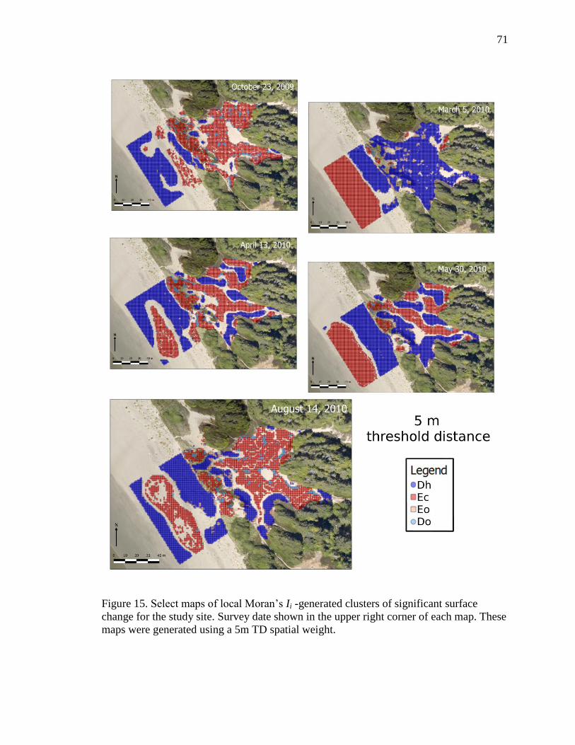
71
Figure 15. Select maps of local Moran’s Ii -generated clusters of significant surface
change for the study site. Survey date shown in the upper right corner of each map. These
maps were generated using a 5m TD spatial weight.

72
The local Moran’s Ii maps for the 1.5 m TD spatial weight (Figure 13) generally
have very little outlier areal coverage and most of the study area is classified as clusters
of Dh or Eh. Erosion dominates in the beach the winter and spring months (i.e., between
October and May) and clusters of deposition build on the upper beach in the incipient
dune zone during this time. Also, between March and May, Ec dominate the foredune
stoss and Dh develop in the foredune lee. These depositional clusters continue to build
through August. The transgressive dune complex shows the most variability with Ec
dominating in October then replaced by Dh by March (with Eo), and linear clusters of Dh
and Ec developing in subsequent surveys (largely aligned with the dominant transporting
wind direction, from WNW). The surface area of Ec is generally greater than Dh (Table
5) except for December, March, and April.
The maps of local Moran’s Ii derived using the 5 m TD spatial weight reveal an
increase the surface area of all significant clusters of change (on average ~70%), with the
outlier values increasing by an order of magnitude (e.g., for the annual Aug-Aug survey,
an increase from 14 to 683 m2). Generally, the spatial trends described above for the 1.5
m TD are continued and expanded, and patterns are smoothed out. The presence of Do
and Eo is more evident in Figure 14 where they occur dominantly in the upper beach,
foredune, and transgressive dune complex with fewer sporadic occurrences in the lower
beach face. Again, the surface area of Eo is greater than that of Do, except for January,
March, and May (when beach erosion dominates). Note also that the area of Dh clusters
is nearly double that of the Eh clusters for March, the largest discrepancy for the dataset.
3.4.2. Geomorphic and sediment volume changes

73
Figures 14 and 15 are based on the original change DEMs for each geomorphic
unit (using basic pixel subtraction described in section 2.1) with application of the 1.5 m
and 5 m TD local Moran’s Ii surfaces to filter out insignificant pixels. Corresponding
values of volumetric changes in each geomorphic unit for each spatial weight TD are also
provided in Table 6.
Table 6. Estimates of statistically significant sediment volume changes using spatial
statistical thresholds. Area normalized values (in brackets) provide an effective depth of
average sediment accretion (+) or erosion (-) within each unit.
Volumetric change from LiDAR baseline (m3) and area-normalized
(m3 m
-2)
1.5 m threshold distance 5 m threshold distance
Survey (Julian Day)
Beach:
4470 m2
Foredune
:
1565 m2
Transgressiv
e Dune:
4285 m2
Beach:
4470 m2
Foredune
:
1565 m2
Transgressiv
e Dune:
4285 m2
September 24 (267)
+572
(+0.128
)
-59
(-0.012)
+61
(+0.014)
+746
(+0.167
)
-31
(-0.020)
+187
(+0.044)
October 23 (296)
+647
(+0.145
)
+11
(+0.065)
-39
(-0.009)
+956
(+0.214
)
+45
(+0.029)
+155
(+0.036)
December 8 (342)
+322
(+0.072
)
+80
(+0.088)
+97
(+0.019)
+483
(+0.108
)
+127
(+0.081)
+221
(+0.052)
January 15 (15)
-162
(-0.036)
+82
(+0.058)
+145
(+0.034)
-133
(-0.030)
+124
(+0.079)
+302
(+0.071)
March 5 (64)
-635
(-0.142)
+136
(+0.072)
+242
(+0.057)
-650
(-0.145)
+159
(+0.102)
+368
(+0.086)
April 13 (103)
+523
(+0.117
)
-17
(-0.062)
+132
(+0.031)
+766
(+0.171
)
+31
(+0.020)
+270
(+0.063)
May 30 (150)
+232
(+0.052
)
+64
(+0.082)
+228
(+0.053)
+365
(+0.082
)
+116
(+0.074)
+348
(+0.081)
July 8 (189)
+627
(+0.140
)
+35
(+0.091)
+8
(+0.002)
+870
(+0.195
)
+198
(+0.127)
+112
(+0.026)
August 14 (226) (Annual total)
+611
(+0.137
)
+100
(+0.128)
+66
(+0.015)
+863
(+0.193
)
+162
(+0.104)
+287
(+0.067)

74
Figure 16. Select geomorphic change maps of the study area, with the survey date shown
in the upper right corner of each map. These maps generated after applying the 1.5m TD
local Moran’s Ii statistics as a significant change threshold.

75
Figure 17. Select geomorphic change maps of the study area, with the survey date shown
in the upper right corner of each map. These maps generated after applying the 5m TD
local Moran’s Ii statistics as a significant change threshold. Circles on the annual
(August) change map indicate areas of interest discussed in section 3.5.3.

76
Annually, both the 1.5 m and 5 m TD spatial weights yielded net increases in
sediment volume of +777 m3 and +1313 m
3, respectively (note that the order of
presenting results for each TD remains constant below) , and normalizing this by surface
area yielded an effective depth of sediment accretion, which was +0.280 m3m-2 and
+0.368 m3m-2. Most of this accretion was in the beach unit (+0.137 m
3 m
-2 and +0.193 m
3
m-2
), which was localized in the upper beach and incipient dune zone. In addition, lobes
of deposition in the lee side of the foredune and downwind of the dominant transport
vector (from WNW) into the transgressive dune complex account for the positive
sediment volumes observed there (Table 6).
In addition to experiencing the highest amount of accretion annually, the beach
surface exhibited the greatest total volumetric change (a general proxy for geomorphic
activity) for both TDs (1282 m3 and 1606 m
3 between the minimum and maximum
points, October and March). Erosion and beach steepening began between December and
January surveys and a low in the sediment volume (-635 m3 and -650 m
3) was
experienced by March, and the onset of summer wave conditions and transporting wind
events (recall the inferred summer wind regime dominance discussed in 1.2) resulted in
accretion after March. Most of the accretion was localized in the upper beach/incipient
dune zone, aided by aeolian sediment transport off the beachface and seasonal vegetation
growth in this area.
The foredune unit experienced deflation immediately after vegetation removal
with the 1.5m TD volumetric response (-59 m3) exceeding that of the 5m TD (-31 m
3).
Recovery was slow with accretion in the lee side of the foredune initially offset by a stoss
side scarp (see March and April change maps, Figures 14 and 15) to the extent that the

77
1.5m TD sediment volume change was negative by April (-17 m3). As with the upper
beach, the return to a positive sediment volume change coincided with the initiation of
the summer wind regime and associated aeolian transport off the beachface (Table 6).
Landward of the foredune, the transgressive dune experienced the least
volumetric change (Table 6). A decline in sediment volume occurs between the
September and October surveys (resulting in a negative volume relative to the LiDAR
survey of -39 m3 for the 1.5m TD), however a mostly regular increase in sediment
volume follows until the May survey. Between the May and July surveys, 220 m3 (1.5m
TD) and 236 m3 (5m TD) are denuded from the transgressive dune complex. Sediment
volumes recover marginally for the annual (August) surveys.
3.5. Discussion
3.5.1. Interpretation of local Moran’s Ii results and their geomorphic relevance
Using the local Moran’s Ii statistics in an exploratory manner reveals a number of
patterns across the study area. First, as discussed in Section 1.1, an intuitive interpretation
of the HH and LL clusters produced by Moran’s Ii for this study are clusters of extreme
deposition and erosion (Dh and Ec), respectively (Figs. 11, 12). However, when
interpreted this way, the difference between the October and March 5m TD local Moran’s
Ii maps indicate a notable shift from an erosive transgressive dune complex to a
depositional one. However, when the same interval is presented as the 5m TD
geomorphic change DEMs (Fig. 16), no such overall change is observable. This can be
explained by the extent of the vertical change data in each map. The beach surface
reflects a steeper winter profile by March with a highly denuded beach face. This area of

78
denudation is absent in the October survey, when a less steep summer beach profile is
still remnant. Thus, in March, there is a much lower “low” point in the elevation change
data, drawing the distribution of data downward, forcing the data in the transgressive
dune complex into a “depositional” setting, relative to the mean of the March data. Thus
care must be taken in interpreting local Moran’s Ii results, and, in the case of this study,
are more useful as both exploratory statistics and as an intermediary step (such as
statistical threshold testing, which would be largely unaffected by a distribution shift).
Implementation of local Moran’s Ii can be useful in exploratory analysis due to
the flexibility in exploring various spatial scales of analysis. For instance, in this study
two different spatial weights (TDs) were applied to identify statistically significant
responses at two different spatial scales a very local (1.5m) threshold that scales with the
saltation process and a larger landform scale (5m). A researcher could examine broader
(landscape) scales by implementing a larger threshold distance, or more specific spatial
scales with knowledge of the modal dimensions of various processes or landforms of
interest. As in Table 5, the 1.5m TD in this study resulted in a “buffering” of extreme
results (i.e., Eh and Dh were less extensive), which can be explained by the smaller
spatial neighbourhood (and thus smaller sample size) utilized to calculate the statistic.
From a geomorphic perspective, however, this may relate to the smaller TD (1.5m) only
producing locally significant changes, more directly a result of a migrating depositional
lobe (see the lee side of the foredune, May and August, Figure 15), rather than broad
scale (5m TD) landform change (note how these lobes are, for the most part, integrated
into broader depositional areas, Figure 16).

79
Recall that depositional and erosional outliers as defined by local Moran’s Ii (Do
and Eo) represent anomalies in otherwise smooth patterns across the study site. These
become more evident in Fig. 14, with the higher TD, as more outliers are revealed. This
is a result of the increased spatial neighbourhood (and thus amount of data) included in
each statistical test. Outliers are predominantly depositional (with the exception of the
March survey, when outliers are largely erosional for reasons described above). The
distribution of outliers is focused in the foredune and transgressive dune and likely
represents localized areas of deposition around sparse vegetation in these areas. In
particular, yellow sand verbena (Abronia latifolia) and sea rocket (Cakile edentula) (Fig.
17) provide low, sparse roughness to produce more uniform Do clusters (e.g., those in the
foredune). Also, big-head sedge (Carex macrocephala)(Fig. 18), which has trailing
rhizomes that often align linearly and stabilize trailing ridges of dunes in the
transgressive dune complex, may be responsible for the elongated Do clusters. Thus local
Moran’s Ii may provide a good first order remotely sensed estimate of the vegetation
characteristics of a study site.

80
Figure 18. Picture taken in August 2010 of the back of the transgressive dune complex,
showing the deflation area upwind of the precipitation ridge, with two yellow sand
verbena plants in the foreground. Note the localized deposition around each plant.
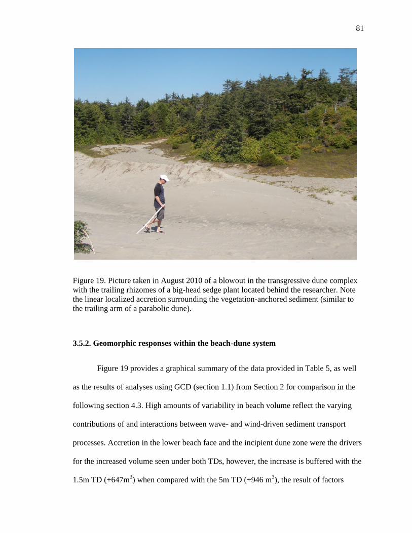
81
Figure 19. Picture taken in August 2010 of a blowout in the transgressive dune complex
with the trailing rhizomes of a big-head sedge plant located behind the researcher. Note
the linear localized accretion surrounding the vegetation-anchored sediment (similar to
the trailing arm of a parabolic dune).
3.5.2. Geomorphic responses within the beach-dune system
Figure 19 provides a graphical summary of the data provided in Table 5, as well
as the results of analyses using GCD (section 1.1) from Section 2 for comparison in the
following section 4.3. High amounts of variability in beach volume reflect the varying
contributions of and interactions between wave- and wind-driven sediment transport
processes. Accretion in the lower beach face and the incipient dune zone were the drivers
for the increased volume seen under both TDs, however, the increase is buffered with the
1.5m TD (+647m3) when compared with the 5m TD (+946 m
3), the result of factors

82
discussed in Section 4.1. The two different TDs agreed well through the erosional period
(October through April) due to the extreme nature of the changes and the spatial contrast
allowing for straightforward identification of significant change (i.e., erosional change
values are extreme relative to the mean). Beach recovery was hindered by the migration
of a rip cell embayment through the study area in May, which steepened the beach profile
and resulted in a net loss of 291 m3 and 401 m
3 of sediment from the beach for the 1.5m
and 5m TDs, respectively. Subsequent beach recovery resulted in sediment volumes that
are not much greater than those surveyed in April (Fig. 19), however the distribution of
sediment changed from swash deposited sediments in the lower beach to aeolian
deposited sediments in the upper beach/incipient dune zone (Figs. 13, 14).
Figure 20. Volumetric change time series in the dune system after the initial LiDAR
survey for each geomorphic unit. Note the values from the two TD spatial weights
generated in this study and the values from the GCD analysis approach from Section 2.
Deflation in the foredune following vegetation removal was largely attributed to
the coincident removal of sediment during the mechanical restoration procedure.
Deposition in the foredune crest and lee contributed to the positive sediment volumes

83
observed through March (+136 m3 and +159m
3 for the 1.5m and 5m TD, respectively),
even when the foredune stoss and toe were extensively deflated and scarped (Figs. 15 and
16) due to high water events and storm activity through late fall and winter. However,
between the March and April surveys, storm activity removed an appreciable amount of
sediment, with the 1.5m TD yielding a negative and the 5m TD yielding a small positive
sediment volume (Table 5). Again, as with the beach, surface deflation was modeled
similarly between the two TDs while deposition is buffered in the 1.5m TD (resulting in
the negative sediment volume for the April survey). This difference can be attributed to:
i) the more marked surface change under erosive conditions being detectable for both
TDs while gradual aeolian buildup went undetected by the smaller threshold distance,
and/or ii) wave eroded surfaces generally being flatter (and less likely to be lost in
interpolation) compared to more hummocky aeolian depositional surfaces. Finally,
aeolian rebuilding occurred after April, with sediment transport into the stoss and lee of
the foredune (+117 m3
and +131 m3 deposited between April and August for each TD)
allowing for scarp recovery and transport over the foredune into depositional lobes. The
upper circle located on the foredune in Figure 16 indicates a conduit for sediment
transport on and through the foredune into the transgressive dune (Figure 20). This was
observed in the 5m TD change maps, but less so in the 1.5m TD change map and is
discussed further in Section 4.3. The lower circle highlights erosion on the stoss side of a
kremholtz Sitka that was not removed in August 2009 (Figure 21).

84
Figure 21. Sand sheet creating a transport pathway through the foredune at the study site.
Photo taken August 2010. Location highlighted as the NW-most yellow circle in Fig. 16
.

85
Figure 22. Photo at the study site showing: i) deflation at the foredune toe in front of the
tree island, visible by the coarser, darker sediment located in the depression, and ii)
accretion in the upwind (i.e., left) side of the tree island, visible by the Sitka Spruce die-
off due to burial. Photo taken August 2010 with the location indicated by the SE-most
yellow circle in Fig. 16.
Initial accretion in the transgressive dune complex is offset by deflation by
October (-100 m3 and -32 m
3 for the 1.5 and 5m TDs, respectively), which, given
appropriate lag time following deflation of the foredune (Figure 19), could be due to a
loss of available sediment for landward transport, exhibiting the coupling between these
two units. Alternating erosional and depositional phases (with a gradual trend of
accretion) occur between January and May (Table 5, Fig. 19), with the patterns
organizing into upwind (toward WNW) deflation feeding downwind accretion. The same

86
lagged deflation pattern discussed above emerges between the April and July surveys,
where deflation of the foredune (-153 m3
and -128 m3 for each TD between March and
April) results in later deflation in the transgressive dune complex (-220 m3
and -236 m3
for each TD between May and July). Final accretion of the transgressive dune complex
occurs predominantly as sediment begins to bypass the foredune, with i) a transport
conduit at the north end of the foredune allowing deposition on the landward side of the
transgressive dune complex, ii) sediment accreting on the eastern edge of the dune
complex, fed sediment from the reworking of upwind well developed depositional lobes
in the lee side of the foredune, and iii) deposition on a transgressing arm in the eastern-
most portion of the dune complex. All this contributes to a modest +66 m3 and +287 m
3
of accretion for the 1.5m and 5m TDs, respectively, over the full year of data. Again, the
1.5m TD is preferential to erosion in the transgressive dune complex (Figures 14 and 15),
with little of the broad pattern of deposition that was observable in the 5m TD.
3.5.3. Comparison of local Moran’s Ii generated geomorphic change thresholds and
those using GCD
Section 2 present an account of the evolution of this coastal dune system, using
the same source data and similar geomorphic maps and volumetric calculations based on
DEM analyses using GCD software. Thresholds generated in that study were based on a
statistical student’s t-test using methodological uncertainties, and they were applied
uniformly over the study area for each DEM. In contrast, thresholds in this study were
applied on a local basis, with each pixel values evaluated for significance in a defined
region of values.

87
Figure 19 shows the volumetric change for each geomorphic unit over the study
period for each TD from this study and the volumetric change from Section 2. In the
beach, the volumetric change over the full year rarely differs between the GCD and 5m
TD results, with a the greatest separation between the two datasets occurring in
December (0.03 m3 m
-2). The 1.5m TD data, however, exhibit the deposition-controlled
“buffer” discussed above, where negative (erosional) sediment volumes are modeled
similarly at the expense of muted response when both the GCD and 5m TD results show
highly positive sediment volumes (e.g., 0.09 m3 m
-2 separating the 1.5m TD volume from
other results on the October survey (Figure 19)). The maps (Figures 6, 14, and 15) all
show similar cycles of erosion and deposition, with the areal extent of upper beach
accretion being more similar between the 5m TD and GCD methods. At the beach-dune
interface, however, there are more marked differences between the local Moran’s Ii and
GCD methods. The deep scarp at the foredune toe, confirmed by photographic evidence
in Section 2, is more pronounced and further landward into the stoss of the foredune at
both TDs.
In the foredune, deflation immediately following vegetation removal, as expected
by sediment removal associated with Ammophila removal, is detected by both local
Moran’s Ii TDs, but not by the GCD method. Afterwards, rapid recovery of the foredune
follows until March, with both TDs reaching sediment volumes of +0.02 m3 m
-2 and+0.04
m3 m
-2 above GCD values for 1.5m and 5m, respectively. The erosion of the foredune
between the March and April surveys, prevalent in the Moran’s Ii results (discussed
above), is minimal in the GCD results (-16 m3
between the two surveys). This is largely
due to the foredune scarp remaining largely unfilled in the local Moran’s Ii volumetric

88
change maps, while nearly gone in the GCD volumetric change maps. Finally,
photographic evidence of features largely undetected by the GCD method show a
sediment transport conduit through the foredune, outlined by the northernmost circle in
Figure 16, which was discussed above (Figure 20). Directly observed in the field, this
feature accreted sediment across the stoss and crest of the foredune, with appreciable
amounts of sediment being deposited as lee-side depositional lobes. Neither the GCD nor
1.5m TD maps convey this feature exhibited in Figure 20, while the 5m TD does. Figure
21, outlined by the southernmost circle in Figure 16, shows the erosion on the stoss side
of a kremholtz Sitka that was not removed in August 2009. Both the 1.5m and 5m TD
capture this erosion; however the GCD method does not.
In the transgressive dune, the volumetric trends of the 1.5m and 5m TDs is almost
identical, however the 1.5m TD consistently shows 0.3 to 0.5 m3 m
-2 less volumetric
change relative to the LiDAR survey. Both patterns and values are nearly identical
between the 5m TD and GCD results, with one distinction being between the months of
December and March. The March change map for the 5m TD (Figure 16) exemplifies
this difference as being one already discussed in Section 5.1. The lowering of the
distribution of data for the 5m TD in January and March due to beach steepening and
erosion lead to more surface change at the study site being extreme relative to the mean,
and thus more significant change was detected than was probably warranted. Thus the
absence of significant volumetric change in the transgressive dune complex observed in
the GCD results is likely more true to the actual volumetric change at the site.
It would appear that the two different spatial thresholds serve two different and
correspondingly useful functions. The 1.5m TD indicates a more conservative (related to

89
both the 5m TD and GCD methods) estimate of volumetric change at the site, with less of
the detrimental data distribution effects discussed in section 4.1. Annual volume changes
are more realistic in a beach dune system that has undergone one year of change
following vegetation removal: foredune sediment volumes became negative after both
mechanical and wave-driven denudation, and annual transgressive dune complex volume
change increased more modestly (after what was likely an erosional or net-zero sediment
volume change prior to restoration, given the likelihood of very low sediment input over
an Ammophila dominated dune). Recall that this spatial scale was utilized to simulate the
outer spatial limit of saltating grains. Thus using the 1.5m TD as a significance threshold
for sediment transport, and thus volumetric transfers over the beach-dune system, appears
more attractive for volumetric estimates than the 5m TD or the GCD method.
In addition, the 5m TD was ideal for feature identification in concurrent data
analyses. Sedimentological features that were confirmed with field reconnaissance, such
as the foredune transport conduit and the erosional hollow (that may develop into a
foredune blowout), were identified in the 5m TD change map (Figure 16). As the 5m TD
was generated to simulate landform development, it provided a useful threshold for
detecting spatially continuous features developed across the study site that remained
undetected in the 1.5m TD or GCD change maps.
3.6. Conclusions
This paper explored the use of spatial statistics for quantifying and examining
volumetric changes and geomorphic response in coastal dune systems using high-
resolution DEMs. The goal of this research was to investigate the properties of spatial
statistics, namely local Moran’s Ii, and how these statistics can be applied to surface

90
change maps generated from DEMs. The use of local Moran’s Ii for generating surface
change results is attractive: they are statistical in nature, they look at a local spatial
neighbourhood surrounding the value under investigation, and significance is inferred
upon rejection of the null hypothesis (i.e., complete spatial randomness). In addition, the
methodology is repeatable, cost-effective, and user friendly, based on freely-available
open source software. Using different TDs, surface change maps were generated using
local Moran’s Ii that identified clusters of statistically significant surface change, and
these maps were used to calculate volumetric change in a coastal system following a
dynamic restoration strategy. The local Moran’s Ii statistics were also useful in
investigating the first order vegetative properties of the study site. When compared to a
DEM analysis using GCD (significance based on the student’s t distribution) using the
same source data, spatial statistics were found to provide both more realistic calculated
volumes at a smaller threshold distance and better highlighting of important spatial
processes at a larger threshold distance not uncovered by the GCD-generated change
DEMs. When properly specified, using spatial statistics for threshold generation provides
a robust, quantitative account of both volumetric change and sedimentological activity in
coastal geomorphology, two important proxies for determining the state of a coastal
system.
3.7. Acknowledgements
The author gratefully acknowledges field and research assistance from Hawley
Beaugrand, Danielle Bellefleur, Mike Collyer, Derek Heathfield, and Nicholas von
Wittgenstein. LiDAR and digital orthophotography was processed by Hawley Beaugrand
in the Hyperspectral LiDAR Research Group lead by Dr. Olaf Niemann in the

91
Department of Geography, University of Victoria. Partial travel funding and logistical
support was provided by Parks Canada Agency, Pacific Rim National Park Reserve.
Fieldwork and data analyses were funded by a Natural Sciences and Engineering
Research Council (NSERC) Discovery Grant to I. Walker, a Geological Society of
America research grant and NSERC Alexander Graham Bell Canadian Graduate
Scholarship to J. Eamer.

92
4. Conclusion
4.1. Summary and conclusions
This thesis provides new methodologies for accurately quantifying geomorphic
change in a coastal setting. The study utilizes data typical to coastal geomorphology (e.g.,
total station, LiDAR) obtained from August 2009 through August 2010 and manipulate it
using easily implemented, cost effective, and repeatable processes. Results were used to
quantify volumetric and surficial change in a discrete coastal system following
devegetation of the foredune, a novel approach to coastal dune restoration. This thesis is
structured around two results sections (2 and 3) derived from data collected between
August of 2009 and 2010 at a beach-dune system located in the Wickaninnish Dunes,
Pacific Rim National Park Reserve, British Columbia, Canada. Each section is prepared
as a manuscript to be submitted for publication in a peer-reviewed journal. Section 2
documented the novel case study of a dynamic dune restoration initiative that involved
mechanical removal of invasive foredune vegetation to improve landscape dynamism.
Section 3 explored the use of spatial statistics for quantifying and examining the same
volumetric change data, with the stated goal of providing improved estimates of
volumetric and surficial change. These sections are bookended with an Introduction
(Section 1) that sets the research context and this section that reviews key findings of the
research.
The purpose of Section 2 was to refine a methodology for identifying multi-
temporal and multi-spatial geomorphic changes between and over all geomorphic units at
the study site and assess the effectiveness of the implemented treatment (dynamic dune

93
restoration) for increasing dune activity. A geostatistical approach using kriging and
open-source software designed for geomorphic change detection in river systems
(Wheaton et al. 2010) was used to model statistically significant changes within beach,
foredune, and transgressive dune geomorphic units separately. This resulted in low
average cross-validation error (0.0058 m) and the method provided a robust account for
uncertainty in each DEM. It was found that the beach maintained a positive sediment
volumetric change of 834 m3 (0.187 m
3 m
-2), largely within the incipient dune zone. This
provided a store of sediment available both as a buffer to wave attack and for further
transport beyond the backshore. In addition, the foredune profile was widened with
increased sediment transported into the lee side of the foredune (200 m3 or 0.128 m
3 m
-2).
Finally, the transgressive dune complex received additional sediment volume (+284 m3 or
0.066 m3
m-2
, largely via extension of depositional lobes from the foredune and accretion
along the downwind edge of the dune complex.
Finally, the dynamic restoration treatment at the site was effective, in terms of
increasing habitat for the SARA-listed Pink sandverbena (Abronia umbellate var
breviflora) via promoting enhanced aeolian activity, improving geomorphic diversity,
and increasing sediment exchanges between landscape units. These responses were not
observed in the control data; either prior to restoration at the study site or at a nearby site
of similar geomorphology where vegetation removal was not complete.
Section 3 utilizes tools provided by the field of spatial statistics, namely local
Moran’s Ii, to assess statistically significant patterns and change at the study site using the
same dataset from Section 2. The purpose of this section was to investigate the
applicability of local Moran’s Ii as applied to DEMs in a coastal setting by comparing this

94
method to the conventional approach of Section 2. Using different TDs, surface change
maps were generated using local Moran’s Ii that identified clusters of statistically
significant surface change, and these maps were used to calculate volumetric change in a
coastal system following a dynamic restoration strategy. The local Moran’s Ii statistics
were also useful in investigating the first order vegetative properties of the study site.
When compared to a DEM analysis using GCD (significance based on the student’s t
distribution) using the same source data, spatial statistics were found to provide both
more realistic calculated volumes at a smaller threshold distance and better highlighting
of important spatial processes at a larger threshold distance not uncovered by the GCD-
generated change DEMs.
4.2. Research contributions and future directions
The major contribution of this research is the development of new methodologies
for determining volumetric and surficial changes in a coastal system in an accurate and
repeatable manner. As discussed above, previous work on meso-scale coastal dune
studies inadequately addresses methodological concerns such as interpolation statistics
and quantification of error, and as such the comparison and synthesis of studies in the
field suffers. Through the expansion of a geostatistical framework provided by Swales
(2002), and application of GCD (section 2) and local Moran’s Ii (section 3) techniques to
data documenting a coastal dune restoration, a statistical basis for error estimation was
created. Comparison of the two methodologies revealed GCD as an ideal simple
approach to geomorphic mapping and error estimation, with local Moran’s Ii providing
more customizable and (given proper utilization) accurate estimates of volumetric change
and surficial properties at the study site. As the properties of local Moran’s Ii were

95
specifically designed for application to this study site, further use in sites of differing
morphologic conditions will provide more insight into the benefits of such an analysis.
In addition to the methodological role, the documenting of a large scale dynamic
dune restoration (a first of its kind in Canada) provides an important contribution to the
coastal geomorphology literature. Increased aeolian activity, geomorphic diversity, and
sediment exchanges across the beach-dune system were observed in both sections 2 and
3, and these factors combine to provide more habitat for the target species. Thus,
restoration success can be inferred based on these factors, however long term monitoring
and maintenance (e.g., manual marram grass removal) are recommended. Also, the
effects of vegetation removal on the foredune resulted in what can be considered an
intuitive morphodynamic response: removal of the surface roughness provided by
vegetation and aeolian sediment transfers were less hindered. Further use of data used in
this study can perhaps be beneficial to development of meso-scale process-response
modeling. Finally, recommendations for future coastal dune management scenarios are as
such:
1. Coastal restoration projects are inherently multidisciplinary, and require
inputs from many facets of science (e.g., ecology, geomorphology, GIS),
2. A strong monitoring program, with baseline control data and long-term
support, is highly beneficial to directing efforts and achieving mandates, and
3. If restoring for active sand surface habitat, the most ideal location for re-
introduction of threatened species is the lee-side of a fully de-vegetated
foredune. This should be adjusted for the burial tolerance of each species.

96
5. References
Agterberg FP. 2004. Georges Matheron: Founder of Spatial Statistics. Earth Sciences
History 23: 205-334.
Andrews BD, Gares PA, Colby, JD. 2002. Techniques for GIS modeling of coastal
dunes. Geomorphology 48: 289-308.
Anselin L. 1995. Local Indicators of Spatial Association-LISA. Geographical analysis
27: 93-114.
Anselin L, Syabri I, Kho Y. 2006. GeoDa: An introduction to spatial data analysis.
Geographical Analysis 38: 5-22.
Anthony EJ, Vanhee S, Ruz M. 2006. Short-term beach-dune sand budgets on the north
sea coast of France: Sand supply from shoreface to dunes, and the role of wind
and fetch. Geomorphology 81: 316-329.
Anthony EJ, Vanhee S, Ruz M. 2007. An assessment of the impact of experimental
brushwood fences on foredune sand accumulation based on digital elevation
models. Ecological Engineering 31: 41-46.
Arens SM. 1997. Transport rates and volume changes in a coastal foredune on a Dutch
Wadden Island. Journal of Coastal Conservation 3: 49-56.
Arens SM, Slings Q, de Vries CN. 2004. Mobility of a remobilized parabolic dune in
Kennemerland, The Netherlands. Geomorphology 59: 175-188.

97
Arens B, Geelen L, Slings R, Wondergem H. 2005. Restoration of dune mobility in the
Netherlands. In: Herrier JL, Mees J, Salman A, Seys J, Van Nieuwenhuyse H,
Dobbelaere I. (Eds.), Proceedings 'Dunes and Estuaries 2005' – International
Conference on Nature Restoration Practices in European Coastal Habitats,
Koksijde, Belgium, 19-23.
Arens SM and Geelen LHWT. 2006. Dune landscape rejuvenation by intended
destabilization in the Amsterdam water supply dunes. Journal of Coastal
Research 22: 1094-1107.
Baas ACW. 2002. Chaos, fractals and self-organization in coastal geomorphology:
simulating dune landscapes in vegetated environments. Geomorphology 48 :
309-328.
Baas ACW, Sherman DJ. 2006. Spatiotemporal variability of aeolian sand transport in a
coastal dune environment. Journal of Coastal Research 22: 1198 – 1205.
Bauer, B., Sherman, D., 1999. Coastal dune dynamics: problem and prospects. In:
Goudre, A.S., Livingston, I., Stokes, J. (Eds.), Aeolian Environments, Sediments
and Landforms. London: J. Wiley and Sons Ltd.
Bauer BO, Davidson-Arnott RGD, Hesp PA, Namikas SL, Ollerhead, J, and Walker IJ.
2009. Aeolian sediment transport conditions on a beach: Surface moisture, wind
fetch, and mean transport rates. Geomorphology 105: 106-116.
Beaugrand HER. 2010. Beach-dune morphodynamics and climate variability impacts on
Wickaninnish Beach, Pacific Rim National Park Reserve, British Columbia,
Canada. Unpublished MSc Thesis, University of Victoria, Canada.

98
Brock JC, Wright CW, Sallenger AH, Krabill WB, Swift RN. 2002. Basis and Methods
of NASA Airborne Topographic Mapper Lidar Surveys for Coastal Studies.
Journal of Coastal Research 18: 1-13.
Bruun P. 1954. Coast Erosion and the Development of Beach Profiles. Beach Erosion
Board Technical Memorandum 44, Washington DC: US Army Corps of
Engineers, 79p.
Bruun,P. 1962. Sea level rise as a cause of shore erosion. Journal of Waterways and
Harbors Division, ASCE, 88: 117-130.
Chapman C, Walker IJ, Hesp PA, Bauer BO, Davidson-Arnott RGD, Ollerhead JO. (in
review). Turbulent Reynolds stress distributions and sand transport responses
over a vegetated foredune. Earth Surface Processes and Landforms.
Chappell A, McTainsh G, Leys J, Strong C. 2003. Using geostatistics to elucidate
temporal change in the spatial variation of aeolian sediment transport. Earth
Surface Processes and Landforms 28: 567-585.
Christiansen MB, Davidson-Arnott, RGD. 2004. Rates of landward sand transport over
the foredune at Skallingen, Denmark and the role of dune ramps. Danish Journal
of Geography 104: 31-43.
D'Antonio C. and Meyerson LA. 2002. Exotic plant species as problems and solutions in
ecological restoration: a sythesis. Restoration Ecology 10: 703-713.
Darke IB, Davidson-Arnott RG, Ollerhead J. 2009. Measurement of beach surface
moisture using surface brightness. Journal of Coastal Research 25: 248 – 256.
99
Darke IB, Walker IJ. 2010. Coastal Geoindicators Monitoring for Climate Change and
Coastal Erosion in Pacific Rim NPR. Report PR-2010-03, Winter 2010.
Darke IB, Walker IJ, Eamer JBR. In review. Geomorphical Considerations for Dynamic
Dune Restoration: Pacific Rim National Park Reserve, British Colombia,
Canada. Earth Surface Processes and Landforms.
Davidson-Arnott RGD. 2005. Conceptual model of the effects of sea level rise on sandy
coasts. Journal of Coastal Research 21: 1166-1172.
Davidson-Arnott RGD, MacQuarrie K, Aagaard T. 2005. The effect of wind gusts,
moisture content and fetch length on sand transport on a beach. Geomorphology
68: 115-129.
Davidson-Arnott RGD, Bauer BO, Walker IJ, Hesp PA, Ollerhead J, and Delgado-
Fernandez I. 2009. Instantaneous and mean aeolian sediment transport rate on
beaches: An intercomparison of measurements from two sensor types. Journal of
Coastal Research SI56: 297-301.
Debruyn W, Deronde B, Fransaer D, Henriet J, Houthuys R, Lancker VV. 2006. Use of
Airborne Hyperspectral Data and Laserscan Data to Study Beach
Morphodynamics along the Belgian Coast. Journal of Coastal Research 22: 1108-
1117.
Delgado-Fernandez I, Davidson-Arnott R, Ollerhead J. 2009. Application of a remote
sensing technique to the study of coastal dunes. Journal of Coastal Research 25:
1160 – 1167.

100
Delgado-Femandez I, Davidson-Arnott RGD. 2011. Meso-scale aeolian sediment input to
coastal dunes: The nature of aeolian transport events. Geomorphology 126: 217-
232.
Eamer JBR, Walker IJ. 2010. Quantifying sand storage capacity of large woody debris
on beaches using LIDAR. Geomorphology 118: 33-47.
Eid B, Calnan C, Henschel M, McGrath B, 1993. Wind and wave climate atlas: Volume
IV the West Coast of Canada. Montreal, Quebec, Canada: Transport Canada.
Retrieved 16 May 2011 from http://www.meds-sdmm.dfo-
mpo.gc.ca/alphapro/wave/TDCAtlas/tdcatlaswc.htm
Englund E. and Sparks A. 1991. Geostatistical Environmental Assessment Software
GEO-EAS 1.2.1 Users Guide. Las Vegas, Nevada: Environmental Monitoring
Systems Laboratory, United States Environmental Protection Agency, 130p.
Gares PA, Wang Y, White SA. 2006. Using LIDAR to monitor a beach nourishment
project at Wrightsville Beach, North Carolina, USA. Journal of Coastal
Research 22: 1206-1219.
Gornitz V. 1995. Sea-level rise: a review of recent past and near-future trends. Earth
Surface Processes and Landforms 20: 7-20.
Grootjans AP, Geelen HWT, Jansen AJM, Lammerts EJ. 2002. Restoration of coastal
dune slacks in the Netherlands. Hydrobiologia 478: 181-203.

101
Heathfield DK, Walker IJ. 2011. Analysis of coastal dune dynamics, shoreline position,
and large woody debris at Wickaninnish Bay, Pacific Rim National Park, British
Columbia. Canadian Journal of Earth Sciences 48: 1185-1198.
Hesp PA. 2001. The beach backshore and beyond. In: Short, A.D. (Ed.), Handbook of
Beach and Shoreface Morphodynamics. Wiley, London, pp. 145-169.
Hesp PA. 2002. Foredunes and blowouts: initiation, geomorphology and dynamics.
Geomorphology 48: 245-268.
Hesp PA, Davidson-Arnott R, Walker IJ, Ollerhead J. 2005. Flow dynamics over a
foredune at Prince Edward Island, Canada. Geomorphology 65 : 71-84.
Houser C, Hapke C, Hamilton S. 2008. Controls on coastal dune morphology, shoreline
erosion and barrier island response to extreme storms. Geomorphology 100:
223-240.
Houser C, Hamilton S. 2009. Sensitivity of post-hurricane beach and dune recovery to
event frequency. Earth Surface Processes and Landforms 34 : 613 – 628.
Houser, C. 2009. Synchronization of transport and supply in beach-dune interaction.
Progress in Physical Geography 33, 733-746.
Jackson DWT, Beyers JHM, Lynch K, Cooper JAG, Baas ACW, Delgado-Fernandez I.
2011. Investigation of three-dimensional wind flow behaviour over coastal dune
morphology under offshore winds using computational fluid dynamics (CFD)
and ultrasonic anemometry. Earth Surface Processes and Landforms, 36: 1113-
1124.

102
Jensen JL, Lake LW, Corbett PWM, Goggin DJ. 1997. Statistics for Petroleum Engineers
and Geoscientists. Upper Saddle River, NJ: Prentice Hall, 390p.
Kollmann J, Brink-Jensen K, Frandsen SI, Hansen MK. 2011. Uprooting and burial of
invasive alien plants: a new tool in coastal restoration? Restoration Ecology 19:
371 – 378.
Krige DG. 1951. A statistical approach to some mine valuations and allied problems at
the Witwatersrand. Master's thesis, University of Witwatersrand.
Lee DS and Shan J. 2003. Combining LIDAR elevation data and IKONOS multispectral
imagery for coastal classification mapping. Marine Geodesy 26: 117-127.
Liu X. 2008. Airborne LiDAR for DEM generation: some critical issues. Progress in
Physical Geography 32: 31-49.
Lynch K, Jackson DWT, Cooper JAG. 2008. Aeolian fetch distance and secondary airfl
ow effects: the infl uence of micro-scale variables on meso-scale foredune
development Earth Surface Processes and Landforms 33: 991–1005. DOI:
Mascarenhas A and Jayakumar S. 2008. An environmental perspective of the post-
tsunami scenario along the coast of Tamil Nadu, India: role of sand dunes and
forests. Journal of Environmental Management 89: 24-34.
Mazzotti S, Jones C, Thomson RE. 2008. Relative and absolute sea level rise in western
Canada and northwestern United States from a combined tide gauge-GPS
analysis. Journal of Geophysical Research 113: 1-19.

103
Mitasova H, Overton M, Harmon RS. 2005. Geospatial analysis of a coastal sand dune
field evolution: Jockey's Ridge, North Carolina. Geomorphology 72: 204 – 221.
Nelson TA, Boots B. 2008. Detecting spatial hot spots in landscape ecology. Ecography
31: 556-566.
Nickling WG and Davidson-Arnott RGD. 1990. Aeolian sediment transport on beaches
and coastal sand dunes. In: Davidson-Arnott, R.G.D. (Ed.), Proceedings of the
Symposium on Coastal Sand Dunes. Ottawa: National Research Council of
Canada, pp. 1-35.
Nordstrom KF. 1990. The concept of intrinsic value in depositional coastal landforms.
Geographical Review 80: 68-81.
Nordstrom KF. 2008. Beach and Dune Restoration. Cambridge, England: Cambridge
University Press, 187p.
Ord JK, Getis A. 2001. Testing for local spatial autocorrelation in the presence of global
autocorrelation. Journal of Regional Science 41: 411-432.
O'Sullivan D, Unwin DJ. 2003. Geographic Information Analysis. New York: Wiley,
436p.
Psuty NP. 1988. Sediment budget and dune/beach interaction. Journal of Coastal
Research, SI 3: 1-4.
Psuty N. 1992. Spatial variation in coastal foredune development. In; Carter, R.W.G.,
Curtis, T.G.F., Sheehy-Skeffington, M.J. (Eds.), Coastal Dunes:

104
Geomorphology, Ecology, and Management for Conservation. Balkema,
Rotterdam, pp.3-13.
Psuty N. 2004. The coastal foredune: a morphological basis for regional coastal dune
development. In: Martinez ML and Psuty N (eds.), Coastal Dunes, Ecology and
Conservation. New York, NY, Springer, pp. 11-27.
Reitz MD, Jerolmack DJ, Ewing RC, Martin RL. 2010. Barchan-parabolic dune pattern
transition from vegetation stability threshold. Geophysical research letters 37,
5p.
Ribeiro JR, Diggle PJ. 2001. geoR: A package for geostatistical analysis. R-NEWS 1:
ISSN 1609-3631.
Riksen M and Goossens D. 2005. Tillage techniques to reactivate aeolian erosion on
inland drift-sand. Soil and Tillage Research 83: 218-236.
Riksen M, Ketner-Oostra R, Van Turnohout C, Nijssen M, Goossens D, Jungerious PD,
Spaan W. 2006. Will we lose the last active inland drift sands of Western
Europe? The origin and development of the inland drift-sand ecotype in the
Netherlands. Landscape Ecology 21 : 431-447.
Rozé F and Lemauviel S. 2004. Sand dune restoration in North Brittany, France: a 10-
year monitoring program. Restoration Ecology 12: 29-35.
Sallenger, Jr. AH, Krabill WB, Swift RN, Brock J, List J, Hansen M, Holman RA,
Manizade S, Sontag J, Meredith A, Morgan K, Yunkel JK, Frederick EB,

105
Stockdon H. 2003. Evaluation of Airborne Topographic LIDAR for Quantifying
Beach Changes. Journal of Coastal Research 19: 125-133.
Saye, S., Vanderwal, D., Pye, K., and Blott, S. (2005). Beach-dune morphological
relationships and erosion/accretion: An investigation at five sites in England and
Wales using LIDAR data. Geomorphology 72: 128-155.
Sherman DJ, Bauer BO. 1993. Dynamics of beach-dune systems. Progress in Physical
Geography 17: 413-447.
Sherman DJ. 1995. Problems of scale in the modeling and interpretation of coastal
dunes. Marine Geology 124: 339-349.
Short AD, Hesp PA. 1982. Wave, beach and dune interactions in Southeastern Australia.
Marine Geology 48: 259-284.
Swales A. 2002. Geostatistical estimation of short-term changes in beach morphology
and sand budget. Journal of Coastal Research 18: 338-351.
Unwin DJ. 1975. An introduction to trend surface analysis. Concepts and Techniques in
Modern Geography. Geo Abstracts Ltd: University of East Anglia, Norwich, 40p.
van Boxel JH, Jungerius PD, Kieffer N, Hampele N. 1997. Ecological effects of
reactivation of artificially stabilized blowouts in coastal dunes. Journal of
Coastal Conservation 3: 57-62.
van Hook SS. 1985. European beachgrass. Fremontia 12: 20-21.
106
Walker IJ, Beaugrand HER. 2008. Coastal Geoindicators Monitoring-Protocol for
Climate Change and Coastal Erosion in Canada’s Pacific Coastal National
Parks. Unpublished report submitted to Pacific Rim National Park Reserve,
Ucluelet, BC. 39p.
Walker IJ, Hesp PA, Davidson-Arnott RGD, and Ollerhead J. 2006. Topographic steering
of alongshore airflow over a vegetated foredune: Greenwich Dunes, Prince
Edward Island, Canada. Journal of Coastal Research 22: 1278-1291.
Walker IJ, Hesp PA, Davidson-Arnott RGD, Bauer BO, Namikas SL, Ollerhead J. 2009a.
Responses of three-dimensional flow variations in the angle of incident wind
and profile form of dunes: Greenwich Dunes, Prince Edward Island, Canada.
Geomorphology 105: 127-138.
Walker IJ, Davidson-Arnott RGD, Hesp PA, Bauer BO, Ollerhead J. 2009b. Mean flow
and turbulence responses in airflow over foredunes: New insights from recent
research. Journal of Coastal Research SI56: 366-370.
Wheaton JM, Brasington J, Darby SE, Sear DA. 2010. Accounting for uncertainty in
DEMs from repeat topographic surveys: improved sediment budgets. Earth
Surface Processes and Landforms 35: 136-156.
Wiedemann AM, Pickart A. 1996. The Ammophila problem on the Northwest Coast of
North America. Landscape and Urban Planning 34: 287 – 299.

107
Wolfe SA, Walker IJ, Huntley DJ. 2008. Holocene coastal reconstruction, Naikoon
peninsula, Queen Charlotte Islands, British Columbia. Geological Survey of
Canada, Current Research 2008-12, 16p.
Woolard JW, Colby JD. 2002. Spatial characterization, resolution, and volumetric
change of coastal dunes using airborne LIDAR: Cape Hatteras, North Carolina.
Geomorphology 48: 269-287.
Zhang K, Witman D, Leatherman S, Robertson W. 2005. Quantification of beach
changes caused by Hurricane Floyd along Florida's Atlantic coast using airborne
laser surveys. Journal of Coastal Research 21: 123-134.