detailed methodology - reason

BUILDING ROADS TO REDUCE TRAFFIC CONGESTION 47

A p p e n d i x B

Detailed Methodology

A. Measures of Congestion A variety of measures of congestion are used in the traffic engineering literature:

1. Freeways: Volume/Capacity Ratio> 1.0 For freeways, congestion is typically measured on a scale relating traffic volume (in the peak hour) to the rated capacity of the facility.i The ‘capacity’ of the facility is defined as the maximum amount of traffic that the facility can carry under prevailing conditions of geometry, traffic mix and location. The practical capacity of modern freeways is about 2,400 vehicles per lane per hour; for older freeways with tight geometrics lower numbers are typical. The so-called ‘volume/capacity ratio,’ V/C, varies from a low of 0 (free flow) to values sometimes greater than 1.0 (severely/heavily congested). Freeways are considered severely congested when the volume/capacity (V/C) ratio is greater than 1.0; for relatively short periods of time, roads can handle more traffic than their rated capacities. The ‘bible’ of traffic level-of-service and congestion is the Highway Capacity Manual.ii In this manual, the “Level of Service” (LOS) provided by the facility refer to both the amount of traffic and the quality of traffic flow. Table B-1 summarizes the descriptions of level of service, which range from “A” (free flow uncongested travel) to “F” (severely or heavily congested flow).

48 Reason Foundation

Table B-1: Levels of Service (LOS)

LOS V/C Ratio Detailed Description A 0.00 – 0.35 Represents the best operating conditions and is considered free flow. Individual users

are virtually unaffected by the presence of others in the traffic stream. B 0.35 – 0.58 Represents reasonably free-flowing conditions but with some influence by others. C 0.58 – 0.75 Represents a constrained constant flow below speed limits, with additional attention

required by the drivers to maintain safe operations. Comfort and convenience levels of the driver decline noticeably.

D 0.75 – 0.90 Represents traffic operations approaching unstable flow with high passing demand and passing capacity near zero, characterized by drivers being severely restricted in maneuverability.

E 0.90 – 1.00 Represents unstable flow near capacity. LOS E often changes to LOS F very quickly because of disturbances (road conditions, accidents, etc.) in traffic flow.

F > 1.00 Represents the worst conditions with heavily congested flow and traffic demand exceeding capacity, characterized by stop-and-go waves, poor travel time, low comfort and convenience, and increased accident exposure.

Although the definitions of specific carrying capacities of freeway lanes have changed in recent years (highway capacities have increased as drivers have become more proficient in driving in congested areas), these changes have not significantly changed the driving conditions of different levels of service.

2. Intersections: Delay > 80 seconds For signalized intersections, the Highway Capacity Manual measures congestion in terms of average delay per vehicle, and ‘levels of service’ are defined based on the average amount of delay. The scale is: LOS A <= 10 Seconds LOS B 11-20 Seconds LOS C 21-35 Seconds LOS D 36-55 Seconds LOS E 56-80 Seconds LOS F >80 Seconds Intersections are considered congested when the average delay exceeds 80 seconds per vehicle. Since many signals are timed on a 2 ½ -3 minute cycle, this is equivalent to requiring the ‘average’ vehicle to wait more than 1 cycle before getting through the light. This definition has also changed in recent years as drivers seem more willing to accept a longer delay; in the 1994 manual the LOS F delay was set at 60 seconds.


3. Travel Time Index (TTI) > 1.18 The above two measures are best suited for analysis of individual facilities but cannot be readily applied to cities. More recently, the Texas Transportation Institute has developed a delay-related index intended to measure the quality of congestion in entire cities. The index is referred to as the Travel Time Index, defined as: TTI = Average travel time in peak hour Average travel time in off-peak hours This index conveniently relates congestion to peak travel times, which people see every day and can understand. For instance, a TTI of 1.25 means that travel times in a given city take 25 percent longer in the peak than in the off-peak. Although no ‘standards’ have been yet agreed upon for what constitutes various levels of congestion using the TTI index, by interpretation travel time is considered severely congested when the TTI exceeds 1.18. This is because a TTI of 1.18 corresponds closely to travel at peak flow, the top of LOS E, which is about 18-20 percent longer travel time than free-flow travel time.

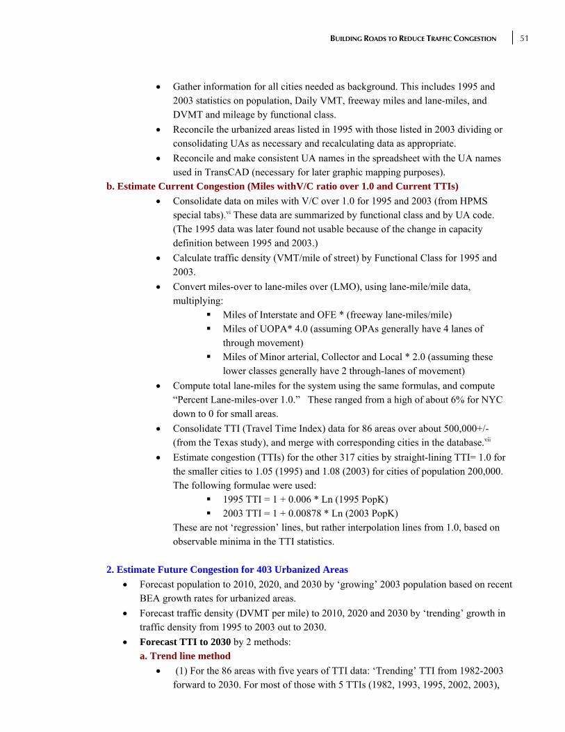
B. General Approach to the Problem In order to use the TTI method for estimating future congestion, the method must be applied to the full range of US cities, then also forecast into the future and related to the magnitude of deficient (LOS F, E, or D) mileage in each city. There are 403 cities in the United States with urbanized area population over 50,000; these typically have federally-mandated Metropolitan Planning Organizations that do formalized (“cooperative, continuing, comprehensive”) transportation planning and have traffic modeling capability. However, comparative TTI measures for congestion statistics are available for only 85 of the largest ones, generally over about 500,000 population, from the annual Texas Transportation Institute congestion survey.iii TTI statistics range from a low of 1.05 for smaller, less congested areas to a high of 1.75 for Los Angeles. These areas are shown schematically in Figure B-1, to the right of the vertical line marked ‘500k.” Most of the areas smaller than 500,000 (to the left of the vertical line) do not have TTI estimates. The Texas Transportation Institute has also estimated congestion reduction costs for 10 Texas cities, using a combination of traffic assignment methods and cost-estimation methods.iv These areas are shown schematically as red stars in Figure B-1. The procedure developed by the Institute uses traffic assignment modeling methods to estimate the additional lane-miles needed to remove ‘level-of-service F’ congestion from the network.


Figure B-1: Schematic for Estimating Congestion Removal Costs

However, this procedure would be cost-and-time prohibitive for the whole US since it would require that about 1000 traffic assignment models be performed for the remaining 395 cities. But an “approximation” methodology can be developed by using a combination of traffic assignment and meta-analysis of other estimates from other similar areas. The methodology operates by consolidating estimates made using the Texas assignment method for some additional areas and then generalizing from these estimates to other similar cities and ultimately to the United States as a whole. In the above figure, the method is analogous to drawing ‘cost lines’ on the figure and then estimating costs for all cities.

C. Detailed Steps in the Methodology Details of the methodology are described in the following steps. 1. Estimate Current Congestion for 403 Urbanized Areas a. Consolidate Data for 403 Urbanized Areas

• Identify 403 urbanized areas (UA) with populations over 50,000. The source of this information is Table HM 71 and HM 72 from the 1995 and 2003 electronic versions of Highway Statistics.v The 2003 version was used as a controlling version for cities over 50,000, since some cities have grown into the group in the past 8 years. Correct any data anomalies found.

City size

TTI for city 500K

1.00

1.50

2.0

$10B

$5B

$1B

City size

TTI for city 500K

1.00

1.50

2.0

$10B

$5B

$1B


• Gather information for all cities needed as background. This includes 1995 and 2003 statistics on population, Daily VMT, freeway miles and lane-miles, and DVMT and mileage by functional class.

• Reconcile the urbanized areas listed in 1995 with those listed in 2003 dividing or consolidating UAs as necessary and recalculating data as appropriate.

• Reconcile and make consistent UA names in the spreadsheet with the UA names used in TransCAD (necessary for later graphic mapping purposes).

b. Estimate Current Congestion (Miles withV/C ratio over 1.0 and Current TTIs) • Consolidate data on miles with V/C over 1.0 for 1995 and 2003 (from HPMS

special tabs).vi These data are summarized by functional class and by UA code. (The 1995 data was later found not usable because of the change in capacity definition between 1995 and 2003.)

• Calculate traffic density (VMT/mile of street) by Functional Class for 1995 and 2003.

• Convert miles-over to lane-miles over (LMO), using lane-mile/mile data, multiplying:

Miles of Interstate and OFE * (freeway lane-miles/mile) Miles of UOPA* 4.0 (assuming OPAs generally have 4 lanes of

through movement) Miles of Minor arterial, Collector and Local * 2.0 (assuming these

lower classes generally have 2 through-lanes of movement) • Compute total lane-miles for the system using the same formulas, and compute

“Percent Lane-miles-over 1.0.” These ranged from a high of about 6% for NYC down to 0 for small areas.

• Consolidate TTI (Travel Time Index) data for 86 areas over about 500,000+/- (from the Texas study), and merge with corresponding cities in the database.vii

• Estimate congestion (TTIs) for the other 317 cities by straight-lining TTI= 1.0 for the smaller cities to 1.05 (1995) and 1.08 (2003) for cities of population 200,000. The following formulae were used:

1995 TTI = 1 + 0.006 * Ln (1995 PopK) 2003 TTI = 1 + 0.00878 * Ln (2003 PopK)

These are not ‘regression’ lines, but rather interpolation lines from 1.0, based on observable minima in the TTI statistics.

2. Estimate Future Congestion for 403 Urbanized Areas

• Forecast population to 2010, 2020, and 2030 by ‘growing’ 2003 population based on recent BEA growth rates for urbanized areas.

• Forecast traffic density (DVMT per mile) to 2010, 2020 and 2030 by ‘trending’ growth in traffic density from 1995 to 2003 out to 2030.

• Forecast TTI to 2030 by 2 methods: a. Trend line method

• (1) For the 86 areas with five years of TTI data: ‘Trending’ TTI from 1982-2003 forward to 2030. For most of those with 5 TTIs (1982, 1993, 1995, 2002, 2003),


trend lines were extended forward to 2030. For just a few, we used four years to ‘slow’ the trend line down. These were mostly large areas that have trends showing congestion ‘slowing’ in recent years.

• (2) For 317 cities with two years of TTI data: We used the 1995 and 2003 estimates of TTI, developed above to ‘trend’ TTIs out to 2030.

b. Regression method • A second method was also used relating TTIs to population and to traffic density.

This method develops a regression model relating 2003 TTI to 2003 Ln PopK and 2003 DVMT/Mi. The idea is that as population grows and traffic density (DVMT/mile) grows, TTIs should increase. The model is:

TTI = 0.1455 Ln (popk) + 0.0000359 (DVMT/mi) t = (19.51) (4.30) R2 = 0.994 N = 86

• To use this model in forecasting TTI, forecasts of DVMT/Mi and population to

2030 from above were then applied to the regression model. For a few smaller areas 1995 DVMT/mi was edited based on missing or clearly incorrect data, usually caused by missing data on the local system, resulting in too-high average DVMT/mi for smaller cities. The editing was done by inserting values based on other similar cities.

• This method also yielded generally reasonable results for the larger areas, but TTIs for the smaller ones tended to be too low, some under 1.0 since the model has few points to work with there, and the model line is steeper than the above lines.

c. Select best estimate • These methods together yielded generally reasonable ‘trend’ TTI numbers. To

resolve the differences between these, we looked at the high and low numbers from above, and then selected the ‘best’ estimate for the 2030 forecast. These were usually the ‘trend’ lines, but for a few larger areas we selected the lower number as being more reasonable. This method produced ‘trend/growth’ forecasts of TTI for each region which look reasonable.

• Forecast LMO (Lane-miles >1.0) for 2030. To complete this task we used four separate methods, which are then averaged and a ‘best estimate’ made.

d. “Percent of system over 1.0” • In this method, the percentage of the (lane-miles) network with lane-miles over

V/C 1.0 is regressed against other ‘rate-like’ variables. The idea here is that an area’s percentage of ‘lane-miles over 1.0’ should increase with traffic density and with rated congestion index. Since this data is available for all 403 areas, the regression is based on all areas.

• The best equation found was: 2003 LMO% = -2.3104 + 0.00039 * DVMT/Mi + 1.8163* TTI

t = (7.38) (2.09)


R2 = 0.199 N = 403

• This estimate is then multiplied by the 2003 network size (lane-miles) to estimate the miles over.

• This model was found to not be very satisfactory. It tended to underestimate the lane-miles-over for large areas, and over-estimate lane-miles over 1.0 for smaller areas.

e. “Growth in population” • In this model ‘2003 lane-miles over’ is regressed directly with area 2003

population. All 403 city data points were used. • The result was:

2003 LMO = 0.254 PopK T = 57.410 R2 = .889 N = 403.000

• This model performed even worse, producing underestimates for the larger areas and overestimates for smaller ones.

f. Elasticity Model, based on DVMT/mi and TTI • In this model, the 2003 “Percent LMO” is regressed against DVMT/mi and TTI.

Then, the regression coefficients are converted to elasticities. This allows us to ‘pivot’ off the current 2003 value in forecasting, thereby using additional information (the current percent LMO) in making the forecast).

• Elasticities for DVMT/Mi and TTI versus Percent LMO are calculated from the mean of the data, using the equation for linear models:

_ _ e = (ΔX/X)/ (ΔY/Y) = (dy/dx)(X/Y) = b (X/Y) For the means of this data base, calculate:

Variable Mean b Elasticity Percent LMO 1.48 DVMT/mi 4672.97 0.00039 1.233 TTI 1.08 1.81629 1.329

The elasticity form of the model is: 2030 %LMO = 2003 %LMO * [1 + 1.233 %Ch in VMT/mi + 1.329 * %Ch in TTI ]

• Then, the estimate of lane-miles over 1.0 is just: 2030 LMO = 2030 %LMO * 2030 Net size (LM)

• This model worked well in forecasting, expanding the current estimate of LMO. However, it does not work well when the current value of LMO is 0, as for small areas since it merely forecasts 0 future LMO for any city with 0 present LMO.


g. Elasticity Model, based on Population • This is an attempt to improve on the straight population model above, using the

elasticity format. The elasticity of lane-miles over 1.0 with respect to population is:

Variable Mean b Elasticity LMO 98.04 Population-K 470.25 0.254 1.218

• The form is: 2030 LMO = 2003 LMO * (1+ 1.218 * % change in PopK)

• This model also worked well, producing similar results to the above. However, it is less useful since it has no policy variables and does not work when the 2003 lane-miles-over is 0.

These four separate methods were then studied carefully, and the best (usually an average of the four results) taken as our best estimate for “2030 Lane-Miles over 1.0”).

3. Estimate ‘Lane-miles needed’ in 2030 to relieve severe congestion Once estimates of future congestion (TTI and Lane-miles over 1.0) have been made for all areas, they must be converted to “lane-miles needed to relieve congestion”. This is done in three steps:

a. Estimate “Lane-miles Needed” from “Lane-miles over 1.0” • “Lane-miles over 1.0” is a measure of congestion for all lanes of congested facilities,

but is not the same measure as ‘lane-miles NEEDED to relieve congestion. Some facilities may need only one additional lane in each direction to relieve congestion, while others may need more than 1.

• “Lane-miles over in 2030” is first spread by functional class, using 2003 data on lane-miles over 1.0 by functional class.

• “Lane-miles over 1.0 in 2030” is then converted to “Lane-miles needed” using: • Interstates and freeways:

Large cities: 6 additional lanes (3 per direction) Mid-sized cities: 4 additional lanes (2 per direction) Smaller cities: 2 additional lanes (1 per direction)

• Other principal arterials: 2 additional lanes • Other roads: 2 additional lanes

b. Estimate “Lane-miles needed’ from assignments in participating areas • The conversion of “Lane-miles over” to “Lane-miles needed” described above does not

consider that areas may be doing additional work in the interim years between 2005 and 2030 to reduce congestion. Nor does it consider how much areas are spreading out or how traffic may divert to widened facilities. Many planners feel that this ‘diverted’ and some ‘induced’ traffic may simply fill up the added lanes. Because of these effects, facilities planned to relieve congestion would have to be larger than initially planned.

• These important factors can be best studied by using traffic assignments of future traffic over a future network that contains improved roads. Ideally, these adjustments


should be made for all 403 areas in the database. However that effort would be time-and-cost prohibitive and would require over 1000 traffic assignments from the cities’ Metropolitan Planning Organizations.

• To avoid this administrative nightmare, a ‘compromise’ method was developed. From the 403 urbanized areas, 44 were asked to participate by running the needed traffic assignments: 10 from the Texas Transportation Institute’s recent Texas Mobility Studyviii (which had already run similar assignments for that study), and 34 additional areas selected to span the range of cities by size and location. These areas ranged from the largest (New York City and Los Angeles) to several small areas (Missoula, MT and Elmira, NY). Some of these did not participate, but ultimately we obtained usable information for 32 areas.

o A list of these 44 areas is in Table B-2 and in Figure B.2. • Each area (other than the 10 in the Texas Study) was contacted and requested to

participate in the study by conducting several long-range traffic assignments using their assignment systems. Basically, these areas were asked to estimate the amount of lane-miles needed to remove LOS F congestion from the future road network, that is, the severe congestion likely to remain AFTER the current long-range plan would be completed in 2030. In essence, they were asked to go beyond their current planning, looking at “what it would take, in terms of additional capacity, to remove severe congestion remaining after the long-range plan is completed.”

Figure B-2: Participating Urbanized Areas


Table B-2: Urbanized Areas in the Texas Mobility Study or Contacted for this Study

Urbanized Area 2003 UA PopK Status of Participation 1. New York 17,170 Requested data received 2. Los Angeles 12,520 Requested data received 3. Chicago 7,702 Did not provide data 4. Miami 5,104 Requested data received 5. Dallas-Fort Worth 4,312 Data available from Texas Mobility Study 6. Washington DC 4,277 Did not provide data 7. San Francisco 4,120 Requested data received 8. Boston 3,988 Did not respond 9. Detroit 3,939 Requested data received 10. Seattle 2,946 Requested data received 11. Atlanta 2,924 Requested data received 12. Phoenix 2,907 Requested data received 13. Houston-Galveston 2,620 Data available from Texas Mobility Study 14. Denver 2,050 Requested data received 15. Cincinnati 1,606 Requested data received 16. San Antonio 1,333 Data available from Texas Mobility Study 17. Columbus 1,195 Refused to participate 18. Salt Lake City 877 Requested data received 19. Austin 757 Data available from Texas Mobility Study 20. Charlotte 725 Requested data received 21. Tucson 720 Requested data received 22. El Paso 629 Data available from Texas Mobility Study 23. Akron 614 Requested data received 24. Raleigh 528 Requested data received 25. Columbia 429 Requested data received 26. McAllen 376 Data available from Texas Mobility Study 27. Spokane 357 Requested data received 28. Little Rock 338 Requested data received 29. Corpus Christi 295 Data available from Texas Mobility Study 30. Durham 281 Requested data received 31. Lincoln 277 Did not provide data 32. Boise 254 Requested data received 33. Eugene 239 Did not respond 34. Lubbock 206 Data available from Texas Mobility Study 35. Laredo 197 Requested data received 36. Evansville 187 Did not provide data 37. Fredericksburg 168 Did not respond 38. Brownsville 156 Did not provide data 39. Binghamton 137 Requested data received 40. Sioux City, IA 108 Data determined from LRP 41.Charlottesville 92 Did not provide data 42. Missoula 74 Data determined from LRP 43. Lewiston ME 69 Did not provide data 44. Elmira NY 57 Did not provide data


• The specific instructions sent to each MPO are as follows:

7-08-05 …., it was nice to talk with you briefly …. I am doing a study I hope you can help me with. The Reason Foundation, a California think-tank, is conducting an assessment of congestion costs and how they might be reduced. One of the issues we are researching is, “What it would take, in terms of additional lane-miles of capacity, to remove the LOS F congestion from urban highway systems?” Since there are over 400 urbanized areas in the United States we can’t cover them all, but we hope to conduct analyses for about 50 cities and then expand the findings to the remainder of US cities. To get a good range of cities we need a variety of urbanized areas, large and small, in the study.

To do the assessment for an urbanized area, we are asking the MPO modeler(s) in each city to conduct a pair of traffic assignments, as follows:

1. Run an ‘all-or-nothing’ (unconstrained paths) future assignment to see what the traffic would be on unconstrained paths.

2. Then ‘expand’ the links that are over 1.0 V/C by enough lanes to reduce the future V/C to 1.0.

3. Then run another equilibrium assignment to verify that the ‘red’ links have been removed.

4. Then summarize the ‘additional lane-miles’ by functional class. 5. Then, if you can, estimate what that additional capacity might cost.

Some regions may have already conducted assessments that are similar and can be readily adapted. I am hoping that you will agree to participate in the study by running these two assignments over the next 2 months. If you can, I’ll send you a more detailed set of instructions, based on Tim Lomax’s study for Texas cities which used this procedure….”

• These initial contacts, in early July 2005, were then followed up by phone calls, suggestions and more detailed instructions. Ultimately 32 urbanized areas provided information (or similar), performing assignments to estimate “lane-miles-needed” using the Lomax method or providing a close approximation. With just a few exceptions, this information was usable.

• Information from the participating areas varied somewhat but generally consisted of estimates of additional lane-miles of capacity, by functional class, needed to remove severe congestion from the long-range plan network.

• This data was carefully compared with the preliminary estimates developed in Step 3a above. As expected, the preliminary estimates were found to be much lower than the results of the assignments, which included long-range plans, urban growth, a specific network, and diversion from slower facilities. Table B-3 shows the results, and the corresponding ‘ratios’ for the 32 urbanized areas, grouped into 9 clusters by size, growth rate, and traffic density.


Table B-3: Clusters by City Size, Growth Rate, and Traffic Density Preliminary

Est. of Lane-Miles Needed

Assignment Est. of Lane-Miles Needed

Cluster Description Urbanized Area Base ST 2030 LMN 2030 LMN Ratio 1 Denver CO 670 4,002 5.97 1 San Antonio TX 500 2,330 4.66 1 Atlanta GA 1,015 2,613 2.58 1 Miami FL 1,707 3,400 1.99 1 Dallas-Fort Worth TX 2,303 3,656 1.59 1 Houston TX 2,753 2,664 0.97 1

Over 915K, Rapid Growth

Seattle-Tacoma WA 735 704 0.96 2 San Francisco CA 1,093 2,261 2.07 2

Over 915K, Med. Growth New York NY 2,123 2,446 1.15

3 Detroit MI 903 2,301 2.55 3 Baltimore MD 445 403 0.91 3

Over 915K, Slow Growth, Low TTI

Cincinnati OH 229 167 0.73 4 Over 915K, Slow

Growth, Med-High TTI

Buffalo-Niagara Falls

NY 187 220 1.17

5 Charlotte NC 209 1,070 5.12 5 Raleigh NC 187 1,204 6.43 5 Austin TX 249 1,168 4.70 5

Between 390K-915K, High Net Density (DVMT/Mi)

Salt Lake City UT 132 477 3.61 6 El Paso TX 93 801 8.61 6 Columbia SC 84 367 4.38 6 Tucson AZ 117 374 3.20 6 Bakersfield CA 73 210 2.87 6

Between 390K-915K, Low Net Density (DVMT/Mi)

Akron OH 34 47 1.37 7 Little Rock AR 101 1,092 10.80 7 Spokane WA 59 518 8.78 7 Corpus Christi TX 61 280 4.57 7 McAllen TX 89 382 4.29 7 Durham NC 78 796 10.21 7

Between 129K-252K

Boise City ID 80 196 2.46 8 Lubbock TX 23 78 3.40 8 Laredo TX 78 239 3.06 8

Between 252K-390K

Binghamton NY 7 16 2.24 11 Missoula MT 9 17 1.89 11

Under 129K, Small Net (DVMT) Sioux City IA 11 19 1.70

*Baltimore, Buffalo and Bakersfield were not contacted. Their long-range plans contained sufficient information.


c. Compute expansion factors for other urbanized areas • This data was then used to compute average expansion factors for similar cities in the

same cluster. The computed expansion factors are:

Table B-4: Expansion Factors for City Clusters Cluster Description Expansion Factor

1 Over 915K, Rapid Growth 2.00 2 Over 915K, Med. Growth 1.40 3 Over 915K, Slow Growth, Low TTI 1.82 4 Over 915K, Slow Growth, Med-High TTI 1.17 5 Between 390K-915K, High Traffic Density (DVMT/Mi > 5658) 4.74 6 Between 390K-915K, Low Traffic Density (DVMT/Mi < 5658) 4.49 7 Between 129K-252K 6.33 8 Between 252K-390K 2.58 9 Under 129K, Unknown Traffic Density (DVMT data missing) 2.50

10 Under 129K, High Traffic Density (DVMT > 2345) 2.00 11 Under 129K, Low Traffic Density (DVMT < 2345) 1.78

• Expansion factors are multiplied by ‘lane-miles needed’ for the other cities to get a revised best estimate of “lane-miles needed”

• As reported in the main text, this totaled 104,022 lane-miles nationwide. 4. Estimate costs to add the lane-miles needed

Once the estimate of “lane-miles needed” was available, the estimation of costs was straightforward. • The total “lane-miles needed” is distributed by functional class using either assignment

results (from participating cities) or using lane-miles-over data by functional class. • Cost per lane-mile from FHWA’s Highway Economic Requirements Study.ix The

average costs per lane-mile for additional lanes are shown in Table B-5. These costs are based on 1997 numbers from the federal highway payment system. For our study, the ‘high cost’ values were applied for 10 cities with more than 3 million population.

• The 1997 costs are adjusted to 2005 using recent trend data from FHWA’s construction cost index. The factor for 1997-2005 is about 15 percent nationwide.

• Unit costs are also adjusted for differences in state construction prices. The HERS report contains information for making this adjustment. The numbers are shown in Table B-6.

Table B-5: 1997 Unit Costs of Urban Highway Construction, Per Lane-Mile, $000

Functional Class igh-Cost Reconstruction

($) ormal-Cost Reconstruction

($) Freew

ays/Expressways ,256 ,550


Other Divided ,910 ,961

Other Undivided ,468 ,268

Table B-6: State cost Factors for Highway Construction (sorted by value)

State 1997 State Highway Construction Cost

Factors

State 1997 State Highway Construction Cost

Factors

State 1997 State Highway

Construction Cost Factors

AK 1.725 OH 1.067 TN 0.896 KY 1.603 GA 1.058 DE 0.887 WA 1.557 LA 1.056 AZ 0.863 HA 1.360 OK 1.023 ND 0.862 NY 1.349 NV 1.017 WI 0.832 MA 1.301 NE 0.981 AR 0.827 VT 1.287 OR 0.977 NJ 0.808 PA 1.257 NC 0.962 MO 0.791 ME 1.215 MT 0.932 WY 0.784 WV 1.165 NM 0.930 KS 0.783 VA 1.161 DC 0.923 RI 0.775 MS 1.150 FL 0.922 IN 0.738 MI 1.141 AL 0.912 TX 0.725 MD 1.131 UT 0.912 SD 0.713 SC 1.115 MN 0.904 IA 0.707 CA 1.096 CO 0.897 NH 0.635 IL 1.076 CT 0.896 ID 0.567

• These costs factors typically show costs higher than average in a few northeast states (although some central and southern states were also above average).

• Unit costs are also adjusted for ‘induced travel’. Induced travel is similar to diverted travel, in that it is thought to be created by the addition of major highway capacity. There are many components of induced travel, including modal shifts, time-of-day shifts, day-of-week shifts, increased trip lengths, increased auto ownership, and possibly increased land use. The magnitude and impact of these components varies widely and indeed some analysts (including this one) are unsure whether induced travel exists at all. However, in this study neither the assignment method nor other adjustments account for these effects, however large they might be. For purposes of this study, we assumed that induced travel adds a maximum of about 15 percent to costs of providing highway capacity in large cities, declining to 0 for smaller cities. The factors are shown in the following table. We did not adjust the ‘mileage needed’ just the costs, since the needed mileage would also be dependent on specific circumstances.


Table B-7: Factors for Induced Travel and Major Bridge Work Population Range Factor for Induced Travel Factor for Major Bridge Work3 million + 1.15 1.10 1– 3 M 1.10 1.05 500K – 1 M 1.05 1.05 <500K 1.00 1.00

• Next, Interstate-OFE costs are also adjusted for the likelihood of major bridge work. In

some, generally larger cities, if major highways were to be expanded then major bridges across rivers and the like would also have to be widened. This factor is set at 10 percent for large cities, and 5 percent for medium cities.

• Costs are also adjusted for the possibility of needed ‘elevated’ or ‘tunnel’ sections. A review of major recent such projects in both the United States and overseas suggests that tunnel costs are about four times surface construction costs, and elevated-section costs about two times surface construction costs. Conservatively, the 4.0 factor is used, but only for a small portion of Interstate-OFE mileage, about 15 percent in larger cities, declining to 2 percent for others. For other cities, no factor is used.

• Finally, for estimating costs in ‘year of construction’ terms, a factor of 30 percent was assumed, this being the average nominal cost increase for projects initiated between 2005 (1.0 factor) and 2030 (1.5 factor).

Table B-8: Cities with Higher Elevated-Section-Tunnel Costs Base Name Percent of UI-OFE System Assumed to

Require Tunnel or Elevated Sections New York-Newark 15.00 Los Angeles-Long Beach 15.00 Chicago 15.00 Philadelphia 5.00 Miami 4.00 Dallas-Fort Worth-Arlington 2.00 Washington 4.00 San Francisco-Oakland 10.00 Boston 15.00 Detroit 10.00 Seattle-Tacoma, WA 10.00 Atlanta 10.00 Phoenix-Mesa 10.00 San Diego 5.00 Houston 5.00 Minneapolis-St. Paul 5.00 Baltimore 3.00 St. Louis 3.00


Table B-8: Cities with Higher Elevated-Section-Tunnel Costs Base Name Percent of UI-OFE System Assumed to

Require Tunnel or Elevated Sections Tampa-St. Petersburg 3.00 Denver-Aurora 3.00 Pittsburgh 3.00 Cleveland 3.00 Portland 7.00 Cincinnati 4.00

5. Uncertainty Analysis of Estimates of Costs to add the Lane-miles needed

• Once costs were calculated, the final spreadsheet was opened in Crystal Ball®,x a graphically oriented forecasting and risk analysis software package. This software uses Monte Carlo simulations to consider a range of inputs rather than an average or an extreme value for particular entries in the database.

• Ranges were used for the following cost factors in the model, to include the induced travel and bridge widening cost multipliers, the elevated or tunnel construction factors, the state construction cost differentials, cost increases over time, and the high and normal variations in construction costs.

• Two distributions were used: triangular (Table B-9) and normal (Table B-10). The distribution-shaping parameters were selected based on a ‘best guess’ approach and are reflected for each factor. Typically, a 10% spread or standard deviation was used.

• The simulation was then run 10,000 times to obtain a distribution of results for the costs to relieve severe congestion. Finally, confidence intervals were determined from this distribution and the sensitivity of the costs to the various input factors was analyzed.

Table B-9: Crystal Ball ® Factors Using a Triangular Distribution Factor Min Value Most Likely Max Value Induced Travel - 3000K+ 1.00 1.15 1.30 Induced Travel – 1000K-3000K 1.00 1.10 1.20 Induced Travel – 500K-1000K 1.00 1.05 1.10 Induced Travel - < 500K 1.00 1.00 1.05 Bridge – 3000K+ 1.00 1.10 1.20 Bridge – 1000K-3000K 1.00 1.05 1.10 Bridge – 500K-1000K 1.00 1.05 1.10 Bridge - <500K 1.00 1.00 1.05 Elevated Hwy-Tunnel 3.00 4.00 5.00 97-05 Cost Increase 1.14 1.15 1.17 State Cost Indices 0.90 1.00 1.10


Table B-10: Crystal Ball ® Factors Using a Normal Distribution Factor Mean Std. Dev. Costs/LM High, Int-Fwy 8,256.00 826.00 Costs/LM High, OPA 4,910.00 491.00 Costs/LM High, MA-COLL-LS 3,468.00 347.00 Cost/LM Norm, Int-Fwy 3,550.00 355.00 Cost/LM Norm, OPA 1,961.00 196.00 Cost/LM Norm, MA-COLL-LS 1,268.00 127.00

D. Methodology for Urban LOS D and E Analysis

The methodology for estimating the cost of removing LOS D and E congestion from the urban system is a simplified version of the LOS F analysis described above. The key differences are that the methodology is state-based, rather than urban-area based, and so estimates are made by applying costs of adding lanes to estimates of mileage at various congestion levels. The specifics of the steps are:

1. Estimate Mileage currently at LOS D and E • Mileage currently (2003) at LOS D and E is available from the Highway Performance

Monitoring System managed by FHWA. The specific tables containing the mileage estimates are Tables HM61, Functional System Length by Volume/Service Ratio, 2003.xi These tables are organized rural/urban, then by functional class and then by V/C ratio. The relevant data are in the columns named “V/C 0.8-0.95,” corresponding closely to the LOS D and E levels of service described above.

• Mileage by functional class is extracted by state. • If summed by class, this data gives reasonably current estimates of mileage of

highways at LOS D and E. The total for the nation, 2003, is 15,853 miles, about 1/3 of the urban mileage at LOS F.

2. Estimate 2030 Mileage at LOS D and E • To estimate future mileage at LOS D and E current mileage must be ‘grown’

somehow. Since we did not ask the MPOs to estimate LOS D and E mileage in 2030, a reasonable approach is to ‘grow’ the 2003 mileage by the same ratio that the urban LOS F miles has been found to grow. This information is available by comparing the 2003 and 2030 LOS F mileage in the urbanized area spreadsheet, and summing the results by state. Typical factors range from 2 to about 5 for most states.

• The estimate of LOS D and E mileage in 2030 is summed by functional class. The result is 42,035 miles, almost 3 times the current number.

3. Estimate 2030 Lane Miles Needed to Remove LOS D and E • The future lane-miles needed to remove LOS D and E is assumed to be two times the

mileage at D and E, since each road section would have to be widened by just two lanes, one on each side. Since the sections are at less than capacity, no more than 2 additional lanes are required.

• This estimate is 84,070 lane-miles.


4. Estimate the Cost of Lane Miles Needed to Remove LOS D and E • The cost of widening is calculated by multiplying the mileage by cost per mile factors.

These factors vary by whether the costs are higher-than typical, or normal cost. The relevant table is:

Table B-11: 1997 Unit Costs, per Lane-Mile, for Highway Reconstruction and Widening Road Type High ($) Normal ($) Freeways/Expressways 8,256 3,550 Other Divided 4,910 1,961 Other Undivided 3,468 1,268

• The source of this table is the federal HERS report mentioned earlier; these are the same costs used as the basis of the urbanized area cost analysis.

• Cost to widen, for each road class, are computed as: Cost = (Lane-mileage needed)*(Cost/lane mile)* State cost factor* Large bridge factor* Tunneling factor* Induced Travel factor* 1997-2005 Price Expansion Factor

• The State Cost Factor is the differential factor for different prices in various states, as described above.

• The Large Bridge Factor, assumed to be 1.05, is intended to account for increased prices of a few major bridge crossings.

• The Tunneling Factor, assumed to be 1.02, is intended to account for some limited mileage that would have to be tunneled or elevated.

• The Induced Travel Factor, assumed to be 1.02, is intended to account for some limited increase in needed mileage and costs caused by traffic created by the widenings. Since these are not fully congested roads, this factor is likely to be small.

• The Price Expansion factor, assumed to be 1.15, is intended to bring price increase up to 2005 from 1997.

Costs are then summed by state. The total estimate is $270.459 billion.

E. Methodology for Rural LOS Analysis This methodology parallels the LOS D and E analysis, with several important differences required by the nature of the unit cost data. The specific steps are: 1. Estimate Current (2003) Rural Congested Mileage

• Rural mileage currently (2003) at LOS F and D-E is also available from the Highway Performance Monitoring System managed by FHWA. The specific tables containing the mileage estimates are also Tables HM61, Functional System Length by Volume/Service Ratio, 2003. Since these tables are organized rural/urban, then by


functional class and then by V/C ratio, the relevant data is in the column named “V/C>0.95,” corresponding closely to the LOS F level of service described above. For LOS D-E, the column is the one named “V/C 0.80-0.95.”

• Mileage in each category by functional class is extracted by state. • If summed by class, this data gives reasonably current estimates of rural mileage of

highways at LOS F. The total for the nation, 2003, is 2,800 miles, very small compared with the urban mileage. For LOS D-E, the summed mileage is 3,985.

2. Estimate Future Rural Congested Mileage

• To estimate future rural congested mileage, current mileage must be ‘grown’ somehow. A reasonable (probably conservative) approach is to ‘grow’ the 2003 mileage by the same ratio that the urban LOS F miles have been found to grow. This information is available by comparing the 2003 and 2030 LOS F mileage in the urbanized area spreadsheet, and summing the results by state. Typical factors range from 2 to about 5 for most states.

• The estimate of Rural LOS F and LOS D-E mileage in 2030 is summed by functional class. For LOS F, the result is 8,177 miles, almost 3 times the current number.

3. Estimate the Lane-Miles needed to Remove Rural Congested Mileage • The future lane-miles needed to remove congested Rural LOS F and LOS D-E mileage

is assumed to be two times the mileage at LOS F or D-E, since each road section would have to be widened by just 2 lanes, one on each side. We assumed that no more than 2 additional lanes are required, one on each side.

• This estimate for LOS F is 16,354 lane-miles. 4. Estimate the Cost to Remove Rural Congested Mileage

• The cost of widening is calculated by multiplying the mileage by cost per mile factors. However, for rural sections these factors vary by functional class, terrain (flat, rolling, mountainous), and high-or-low cost. The relevant table is:

Table B-12: Unit Costs for Rural Highway Reconstruction/Widening, per Lane Mile ($000)

Functional Class/Terrain

Terrain High Cost Reconstruct + Add ($)

Normal Cost Reconstruct + Add ($)

Flat 558 558 Rolling 653 653

Rural Interstate

Mountainous 752 752 Flat 704 704 Rolling 728 728

Rural - Other Principal Arterial

Mountainous 1,036 1,036 Flat 611 611 Rolling 665 665

Rural - Minor Arterial

Mountainous 899 899 Flat 538 538 Rolling 590 590

Rural - Major Collector

Mountainous 789 789


• The source of this table is also the federal HERS report mentioned earlier; these are similar costs as urbanized area costs, but are much lower, by three-quarters, typically, reflecting the lower cost of construction in rural areas.

• To use the table, we must estimate, for each state, whether it is ‘rolling, mountainous, or flat’ in character. However, inspection of the table shows that the ‘costs’ are the same for high and low-cost construction, so that factor is not needed. The following table summarizes these assumptions (showing which states were assumed to be ‘flat, rolling, or mountainous’):

Table B-13: Rural Cost Factors and Terrain Types State State

Code 97 cost factors

Terrain 1Flat

2Rolling 3 Mountainous

Rural Lane-Miles Over 1.0

Growth to 2030

Alabama AL 0.912 1 3.85 Arizona AZ 0.863 1 3.00 Connecticut CT 0.896 1 4.29 Dist. of Columbia DC 0.923 1 2.83 Delaware DE 0.887 1 2.30 Florida FL 0.922 1 3.00 Georgia GA 1.058 1 5.95 Iowa IA 0.707 1 4.48 Kansas KS 0.783 1 5.00 Louisiana LA 1.056 1 1.53 Maryland MD 1.131 1 1.50 Michigan MI 1.141 1 3.54 Minnesota MN 0.904 1 2.28 Mississippi MS 1.150 1 1.45 North Dakota ND 0.862 1 3.13 Nebraska NE 0.981 1 4.91 New Jersey NJ 0.808 1 4.22 Ohio OH 1.067 1 1.92 Oklahoma OK 1.023 1 4.50 Rhode Island RI 0.775 1 1.41 South Carolina SC 1.115 1 3.38 South Dakota SD 0.713 1 2.37 Texas TX 0.725 1 2.92 Wisconsin WI 0.832 1 1.75 Arkansas AR 0.827 2 3.89 California CA 1.096 2 2.62 Illinois IL 1.076 2 1.96 Indiana IN 0.738 2 3.26 Kentucky KY 1.603 2 2.79 Massachusetts MA 1.301 2 1.60 Maine ME 1.215 2 6.05 Missouri MO 0.791 2 2.10 North Carolina NC 0.962 2 3.29 New Mexico NM 0.930 2 3.49


Table B-13: Rural Cost Factors and Terrain Types State State

Code 97 cost factors

Terrain 1Flat

2Rolling 3 Mountainous

Rural Lane-Miles Over 1.0

Growth to 2030

Nevada NV 1.017 2 3.00 New York NY 1.349 2 0.69 Oregon OR 0.977 2 3.09 Pennsylvania PA 1.257 2 2.29 Tennessee TN 0.896 2 2.29 Virginia VA 1.161 2 2.49 Washington WA 1.557 2 2.04 Alaska AK 1.725 3 2.00 Colorado CO 0.897 3 3.00 Hawaii HA 1.360 3 3.17 Idaho ID 0.567 3 2.01 Montana MT 0.932 3 5.00 New Hampshire NH 0.635 3 2.15 Utah UT 0.912 3 3.00 Vermont VT 1.287 3 3.07 West Virginia WV 1.165 3 2.90 Wyoming WY 0.784 3 4.04 • The cost to widen, for each road class, are computed as:

Cost = (Lane-mileage needed)*(Cost/lane mile)* State cost factor* Large bridge factor* Tunneling factor* Induced Travel factor* 1997-2005 Price Expansion Factor

• The State Cost Factor is the differential factor for different prices in various states, as described above.

• The Large Bridge Factor, assumed to be 1.05, is intended to account for increased prices of a few major bridge crossings.

• The Tunneling Factor, assumed to be 1.02, is intended to account for some limited mileage that would have to be tunneled or elevated.

• The Induced Travel Factor, assumed to be 1.02, is intended to account for some limited increase in needed mileage and costs caused by traffic created by the widenings. Since these are rural roads this factor is likely to be small.

• The Price Expansion factor, assumed to be 1.15, is intended to bring price increase up to 2005 from 1997.

Costs are then summed by state. For LOS F, the total estimate is $14.198 billion, a fraction of the urban estimates. For LOS D-E, the total is $19.7 billion.


F. Methodology for Benefit/Cost Assessment The methodology used for estimating benefits of improved travel speeds is the traditional Benefit/Cost method that was, for many years, the mainstay of project assessment. The method works by quantifying, in dollar terms, the value of 3 major ‘user benefits’ of transportation improvement: travel time savings, accident reductions, and reductions in vehicle operating costs. These are then compared with the amortized (annual) cost of the project. The specific steps are:

• Travel time savings are defined as TTS = (Difference in VHT)*Value of time, per hour

The value of time is traditionally taken as about half the wage rate, or about $10/hr in current dollars.

• Accident cost savings are defined as: ACCS = (Difference in VMT)*accident rate/vmt * $cost of an accident Accident rates vary by road class, but nationally the overall death rate is about 1.5 deaths per 100 million vehicle miles. The FHWA used $3 million as the ‘value’ of a life saved.

• Operating cost savings are computed as: OCCS = (Difference in VMT)* Operating cost per mile.

Operating cost per mile is now about 60 cents, weighting trucks and cars. To estimate cost per hour of delay saved, the procedure is:

• Estimate the average number of commuters for each region, between 2003 and 2030.

Commuters = (Pop03+Pop30)/2 * (commuter/pop factor, from the 2000 census). • Estimate each region’s median commute time, from the 2000 Census. • Estimate Ave Annual Delay Saved

Delay Saved = (Ave Commuters) *500 commutes/year *median travel time *(TTI2030 – min(1.18, TTI2003))

• Estimate Cost per hour of delay saved Cost/hour of delay saved = (Total Est cost)/25 years/Ann Delay Saved

detailed methodology - reason

Documents