detailed kinetic analysis of oil shale pyrolysis tga...
TRANSCRIPT

1
Detailed kinetic analysis of oil shale pyrolysis TGA data
Pankaj Tiwari and Milind Deo*
Department of Chemical Engineering, University of Utah, Salt Lake City, Utah, 84102, USA
Abstract
There are significant resources of oil shale in the western United States, which if exploited in an
environmentally responsible manner would provide secure access to transportation fuels.
Understanding the kinetics of kerogen decomposition to oil is critical to designing a viable process.
A dataset of thermo gravimetric analysis (TGA) of the Green River oil shale is provided and two
distinct data analysis approaches – advanced isoconversional method and parameter fitting are
used to analyze the data. Activation energy distributions with conversion calculated using the
isoconversional method (along with uncertainties) ranged between 93 kJ/mol to 245 kJ/mol. Root
mean square errors between the model and experimental data were the lowest for the
isoconversional method, but the distributed reactivity models also produced reasonable results.
When using parameter fitting approaches, a number of models produce similar results making
model choice difficult. Advanced isoconversional method is better in this regard, but maybe
applicable to a limited number of reaction pathways.
Introduction
Oil shale offers promise as a significant domestic oil source. The Green River formation contains
proven vast amounts of oil shale spread among the states of Colorado, Utah and Wyoming.1-3
Mahogany zone is one of the richest oil zone intervals.4 The organic portion of the shale, known as

2
kerogen, undergoes chemical decomposition on thermal heating or retorting to produce a liquid
(shale oil). Retorting of oil shale can be performed in different environments. Pyrolysis is a process
of heating oil shale in an inert environment. Primary products of pyrolysis are liquid, gas and coke.
The extent of decomposition (yield) and the quality of pyrolysis products depend on the
composition of the source material,5-7 the temperature-time history,8,9 pressure,10-12 residence time
(secondary reaction)13,14 and presence of other reactants such as water,15-18 methane,19 O2,20 CO2,
21
etc. Because of the chemical composition of the oil produced, moderate to significant upgrading
(nitrogen removal and/or hydrogen addition) may be required to convert the oil into a refinery
feedstock.22-24 Producing shale oil of desirable characteristics (low heteroatom content and
molecular weight, and high hydrogen) requires an understanding of the decomposition
mechanisms and kinetic parameters - activation energy E, pre-exponential factor A and the reaction
model ƒ(α).
TGA analysis of oil shale pyrolysis has appeared in the literature; Colorado oil shale (Green River
Formation),25-27 Spanish oil shale (Puetrollano),7 Chinese oil shales,28-30 Pakistani oil shale,31
Jordanian oil shale,21 Moroccan oil shale,32 etc. Elemental analysis and pyrolysis kinetics of oil
shales from all over the world were summarized by Nuttal et al. (1983)5 who observed that there
were considerable variations in the kinetic parameters of the different shales. A number of
researchers have derived relatively simple but effective kinetic expressions for oil evolution during
the pyrolysis of Green River and other oil shales based on first-order reaction,33,34 consecutive
first-order reactions,35 parallel first-order reactions,36 and logistic or autocatalytic mechanisms37.
Campbell et al. (1978)34 postulated a first-order decomposition mechanism for the pyrolysis of
Colorado oil shale and reported an activation energy of 214.4 kJ/mol and a frequency factor of
2.8E13 s-1. Leavitt et al. (1987)36 proposed two parallel first-order lumped reactions and, obtained

3
activation energies of 191.02 kJ/mol for temperature above 3500C and 87 kJ/mol for temperature
below 3500C. A controversial two-step mechanism has also been proposed by Braun and Rothman
(1975).38 Burnham (2010)39and Burnham (1995)15 have argued convincingly by using multiple
sets of data that this two step decomposition mechanism is not appropriate for oil shale pyrolysis.
More complex kinetic analysis procedures have also been used in deriving kinetics of
decomposition of oil shales.6,40-42 It has also been reported that kinetics parameters obtained using
one apparatus do not agree well with those derived using a different system. Burnham (2010), 39
notes that these differences are primarily due to the use of poor kinetic analysis methods.
The kinetic analysis round table43-47 convened to study the kinetics of reactions involving complex
solid materials concluded that it was inappropriate to use a single heating rate and a prescribed
kinetic model to derive kinetic parameters. The basic flaw in methods which followed this
procedure was that they resulted in activation energies that were heating rate dependent. By using
a variety of computational methods, the panel observed that isoconversion and multi-heating
methods were particularly useful in describing kinetics of complex material reactions.43 Burnham
and Braun (1999)48 reviewed various kinetic analysis approaches for obtaining kinetic parameters
for reactions involving complex materials. They argue for the use of well chosen models that are
able to fit the data and extrapolate beyond the time-temperature range of the data. For complex
materials such as kerogen, generalized distributed reactivity models were found to be suitable.
When studying the oil shale pyrolysis data, Burnham and Braun (1999)48 use modified Friedman
and the modified Coats and Redfern methods while also employing the discrete activation energy
model. Burnhan and Dihn (2007)49 also compared the isoconversional methods to models obtained
using nonlinear parameter estimation. They concluded that reactivity distribution of parallel
reactions involving complex materials can be modeled effectively using either the isoconversional

4
methods or parameter fitting approaches; however, they observed that the isoconversional methods
are fundamentally inappropriate for use in modeling competing reactions.
Most of these studies recommended the use of distributed reactivity or similar methods, where, the
reaction rate is inherently independent of heating rates. Variations in the application of these
concepts exist in the literature,49-52 particularly in the manner in which the equations are solved.
One the first applications of the isoconversion method, based on the differential form of the rate
equation53 is the Friedman method. Modifications and applications to different complex materials
have been reported.48,50,54 A general application of this concept is the postulation of a model-free
isoconversional method,55 where a functional form of the reaction model is not pre- supposed.
Extensions of this basic theory in the form of advanced isoconversional method have been applied
to a number of complex solid materials.54,56,57 A comprehensive suite of kinetic analysis models
based on the concepts discussed by Burnham and Braun48 is available for use (Kinetic05).
The purpose of this paper is to provide a complete TGA dataset for the pyrolysis of Green River
oil shale, and to compare the performance of the different kinetic models in being able to match
the data. Advanced isoconversional models have not seen widespread use perhaps due to their
relative computational complexity. The methodologies for implementation of these models allow
computations of parameter uncertainties as well. The sophisticated parameter fitting methods are
intuitive and easily implemented. However, selection of a unique model from a number of
available choices is sometimes difficult. In this paper, the root mean square errors between the
experimental and modeling data are compared. Selection of a model has real consequences on
process predictions – hence it is important to understand the advantages and disadvantages of
using different models.

5
Experimental Section
The oil shale samples obtained from the Utah Geological Survey were crushed and screened to 100
mesh (1.49 x10⁻⁴ m) size particles. The samples were from the Mahogany zone of the Green River
formation. The CHNSO (carbon, hydrogen, nitrogen, sulfur ad oxygen) elemental analyses of the
sample were performed using LECO CHNS-932 and VTF-900 units and results are summarized in
the Table 1. The table lists the values along with the standard deviations. The elemental analysis
shows that oil shale obtained is Type I on Van Krevelen classification diagram based on the H/C
ratio (1.1) and O/C ratio (0.67).58 The crushed samples were dried for four hours at 1000C to
remove moisture. There was no significant weight loss during drying, and hence the samples were
used as received after screening to 100 mesh. To study the reaction kinetics, a TGA instrument
(TA Instruments Q-500) was used for the entire temperature range of kerogen decomposition in N2
(pyrolysis) environment. Non-isothermal TGA offers certain advantages over the classical
isothermal method because it eliminates the errors introduced by the thermal induction period.
Non-isothermal analysis also permits a rapid and complete scan of the entire temperature range of
interest in a single experiment.
Results and Discussion
Experimental Data
Non-isothermal TGA experiments were performed at heating rates between 0.50 - 500C/min for the
decomposition of the crushed and un-dried oil shale samples (20-30 mg). Weight loss data along
with derivatives are shown in Figure 1 for seven (7) heating rates. The mass and temperature
measurements in the instrument were calibrated periodically and confirmed with a standard
material, calcium oxalate. Excellent reproducibility was observed in the mass loss curves. The
6
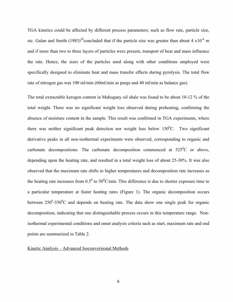
TGA kinetics could be affected by different process parameters; such as flow rate, particle size,
etc. Galan and Smith (1983)26concluded that if the particle size was greater than about 4 x10⁻⁴ m
and if more than two to three layers of particles were present, transport of heat and mass influence
the rate. Hence, the sizes of the particles used along with other conditions employed were
specifically designed to eliminate heat and mass transfer effects during pyrolysis. The total flow
rate of nitrogen gas was 100 ml/min (60ml/min as purge and 40 ml/min as balance gas).
The total extractable kerogen content in Mahogany oil shale was found to be about 10-12 % of the
total weight. There was no significant weight loss observed during preheating, confirming the
absence of moisture content in the sample. This result was confirmed in TGA experiments, where
there was neither significant peak detection nor weight loss below 1500C. Two significant
derivative peaks in all non-isothermal experiments were observed, corresponding to organic and
carbonate decompositions. The carbonate decomposition commenced at 5250C or above,
depending upon the heating rate, and resulted in a total weight loss of about 25-30%. It was also
observed that the maximum rate shifts to higher temperatures and decomposition rate increases as
the heating rate increases from 0.50 to 500C/min. This difference is due to shorter exposure time to
a particular temperature at faster heating rates (Figure 1). The organic decomposition occurs
between 2500-5500C and depends on heating rate. The data show one single peak for organic
decomposition, indicating that one distinguishable process occurs in this temperature range. Non-
isothermal experimental conditions and onset analysis criteria such as start, maximum rate and end
points are summarized in Table 2.
Kinetic Analysis – Advanced Isoconversional Methods

7
It has been noted in the earlier literature that kerogen is a cross-linked, high molecular weight
solid.59,60 During pyrolysis, bonds are broken, leading to multiple reactions. As described earlier,
one peak was observed in the organic decomposition temperature range. Consequently, globally
single stage decomposition was assumed in deriving kinetic rate expressions.
Kerogen Decomposition Products
Advanced isoconversion methods or sophisticated parameter estimation methods would be
appropriate for the analysis of kinetics of decomposition of complex materials like kerogen.43,49
The salient features of these methods are discussed here.
The conversion of solid matter in shale (kerogen) to products from TGA weight loss data is
defined as,61
WW
WW t
0
0
In general, the rate of decomposition can be expressed using the non parametric kinetic equation
)()( fTf
dt
d
Using Arrhenius expression leads to the following,
)()()( )( feAfTf
dt
d tRT
E
Isoconversional methods are specifically designed to address deficiencies in variable heating rate
analyses.43 Advanced model-free isoconversion method has been used in this paper. The concepts
(3a)
(2)
(1)
8
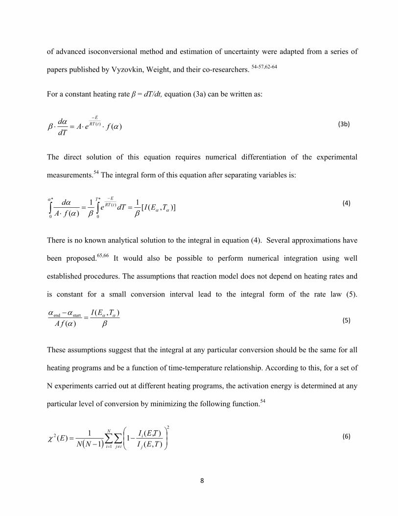
of advanced isoconversional method and estimation of uncertainty were adapted from a series of
papers published by Vyzovkin, Weight, and their co-researchers. 54-57,62-64
For a constant heating rate β = dT/dt, equation (3a) can be written as:
)()( feAdT
d tRT
E
The direct solution of this equation requires numerical differentiation of the experimental
measurements.54 The integral form of this equation after separating variables is:
*
0
)(*
0
)],([11
)(
TtRT
E
TEIdTefA
d
There is no known analytical solution to the integral in equation (4). Several approximations have
been proposed.65,66 It would also be possible to perform numerical integration using well
established procedures. The assumptions that reaction model does not depend on heating rates and
is constant for a small conversion interval lead to the integral form of the rate law (5).
),(
)(startend TEI
fA
These assumptions suggest that the integral at any particular conversion should be the same for all
heating programs and be a function of time-temperature relationship. According to this, for a set of
N experiments carried out at different heating programs, the activation energy is determined at any
particular level of conversion by minimizing the following function.54
N
i ij j
i
TEI
TEI
NNE
1
2
2
),(
),(1
1
1)(
(4)
(5)
(6)
(3b)

9
Where the subscripts i and j represent two experiments performed under different heating
programs. The trapezoidal rule is used to evaluate the integral numerically and the minimization
procedure is repeated for each value of α to find the dependence of activation energy on the extent
of conversion. The activation energy distribution obtained in equation (6) can be used to determine
[A•ƒ(α)] as a function of α. The confidence intervals for the activation energies and for the values
of A•ƒ(α) can be calculated using the statistical approach described.54,64
The experimental rate and conversion data can be reconstructed based on the model parameters
using equation (7) below.
iii TR
EfA
dT
d
,,
)(lnln
A MATLAB program utilizing the function ODE45 was used to solve the above ordinary
differential equation. E (α) and A•ƒ(α)] which were inputs to the MATLAB program were
obtained using the isoconversional analysis described above.
The kinetic models can be used to extrapolate to non-experimental rates. Slow pyrolysis that is
likely during in-situ oil shale production and high rates of flash pyrolysis are of interest. The
assumptions of the isoconversion method (Equation (5) allow calculating the temperature to reach
a level of conversion at extrapolated heating rates using the following mathematical equivalency,56
j
j
i
i TEITEI
),(),( ,,
The equation above was used to estimate the temperature at which the material starts to convert.
The procedure for reconstruction was then used to obtain conversions and rates at extrapolated
(7)
(8)

10
conditions. One of the advantages of using the advanced isocoversional approach is that
uncertainties in E values can also be estimated.
Kinetic Analysis - Advanced Parameter Fitting Approaches
Results from other parametric fitting models were compared with those obtained with advanced
isoconversional method. The Kinetic05 package developed by Braun and Burnham at Lawrence
Livermore National Laboratory and supplied by GeoIsoChem is capable of obtaining kinetic
parameters of a variety of models. These include the power law and the distributed reactivity
models. TGA or other thermal analysis data can be used. Distributed reactivity model options
include the Friedman-based isoconversional method, Gaussian and Weibull distributions, and a
few others. The application of these models were discussed by Burnham and Braun (1999)48 for
different complex materials. In Kinetic05, the model parameters are refined by minimizing the
residual sum of squares between observed and calculated reaction data by using nonlinear
regression. The details of mathematical formulas and solution procedures have been published
previously.48
Kinetic Analysis Results – Advanced Isocoversional Method
The TGA data were normalized from zero to one prior to analysis. The temperature at which the
derivative of weight loss starts to rise was chosen as the zero conversion point, and the temperature
at which the weight derivative returned to the base line was the end point. Isokin, a package
developed at the University of Utah54 was used for the calculation of the distribution of activation
energies and other kinetic parameters. Distributions in kinetic parameters, E and A·ƒ(α) were
determined as functions of conversion.

11
The confidence interval estimation was performed by using different number of heating rates
and/or different combinations of heating rates. Uncertainties were calculated for 10 conversion
intervals for different cases (Figures 2, a-d). Uncertainty values increased when fewer rates were
used. When heating rates spanning the wider range (for example 500C/min and 0.50C/min) were
included in sparse data sets, the uncertainties were generally lower. Figure 3-1 shows activation
energy distribution (as a function of conversion) and associated uncertainties when all the seven
heating rates were employed. Figure 3-b shows A·ƒ(α) as a function of conversion. Activation
energies ranged from 93 - 245 kJ/mol. The values of A·ƒ(α) varied from 1.42E6 - 4.46E16 min-1.
The kinetic parameters estimated in this work are consistent with those observed by others for
Green River oil shale.33,34 For Kukersite shales, which was considered a “standard” because of
reproducibility, the activation energies ranged from 210 kJ/mol to 234 kJ/mol.48 The values of
activation energies reported in this work of about 93 kJ/mole to 245 kJ/mol are lower at lower
conversions.
It is argued (Vyazovkin, 2003)67 that the variation in activation energy for the decomposition of a
complex material is caused by the fact that the overall rate measured by thermal analysis is a
combination of the rates of several parallel reactions, each of which has its own energy barrier, and
hence an activation energy. The effective activation energy derived from these global rate
measurements becomes a function of the individual activation energies.
Advanced isoconversion method provides combined pre-exponential factor and reaction model as
function of conversion. The values of pre-exponential factor A can be calculated after assuming a
reaction model (order, functionality, etc.). For example, the Friedman method assumes a first-order
reaction, and using the functionality of (1-α) for f(α), A can be calculated. A graphical
implementation of the Friedman approach also yields E(α) and A as functions of conversion. The

12
comparison of kinetic parameters obtained from Isokin first-order model and Friedman graphical
method are depicted in Figure 4. The agreement between kinetic parameters obtained using the two
approaches is excellent. The results support that thermal decomposition pyrolysis of Mahogany oil
shale is globally a first-order process. This is also confirmed by observing the Constable plot, that
examines the relationship between logarithm of A and E.68 The linear (or near-linear) profile in the
Constable plot may be adequate62 to confirm the order of the reaction. The Constable plots shown
in Figure 5 are remarkably linear confirming the order to be unity for both the approaches
employed.
The distributions of E and A·f(α) were used in model equations to recreate the experimental data.
A MATLAB code with the ODE45 solver was used in the calculations. In the practical
implementation of the code, temperature was the dependent variable. Results of the model
comparisons with the experimental data are shown in Figure 6. The agreement between the model
and the experimental data is good over most of the conversion range, and for all the rates. The
experimental data at 10oC/min were used as basis to calculate the conversion profiles for rates at
which experimental data was not available. Extrapolated profiles at rates ranging from 0.010C/min
to 5000C/min are shown in Figure 7. At slow heating rates, decomposition begins at lower
temperatures while in the fast pyrolysis, the products are released at higher temperatures.
Simulated decomposition rates and onset temperatures shift to higher temperatures at higher
heating rates. The extrapolated results are not all consistent with some experimental results. To
explain all aspects of the extrapolated profiles, introduction of reaction initiation type
mechanisms14,69 proposed by a few researchers may have to be considered.
Kinetic Analysis Results – Advanced Parameter Fitting Models
13
The models from Kinetic05 used for comparison purposes are listed in Table 3. Table 3 also shows
the parameters obtained. The power law model was applied in two cases; first-order and nth-order.
In the latter case, optimal values of n, E and A were obtained using non-linear regression. The nth-
order reaction model is mathematically equivalent to Gamma distribution.70 The Gaussian
distribution approach used by Braun and Burnham (1987)71 was also used with the first and the nth-
order models. Discrete reactivity distribution models are based on different combinations of A and
E assuming the reaction to be first-order. Three different cases were used in this work and the
results were compared;
1. Fixed E-spacing,
2. Initial A-range and fixed E-spacing
3. Constable relationship for A and E - (ln(A) = a + bE).
The distributions of activation energies from discrete models are shown in Figure 8. The three
different approaches produced different kinetic parameters. Use of Weibull distribution is another
parameter fitting method used extensively for petroleum source rocks by Lakshmanan et al.
(1994).72 Isoconversional method in Kinetic05 is based on the first-order Friedman-type of
analysis. The distribution of activation energies obtained using this approach in Kinetic05 is
almost identical to the distribution obtained using the advanced isoconversional method (Figure 4).
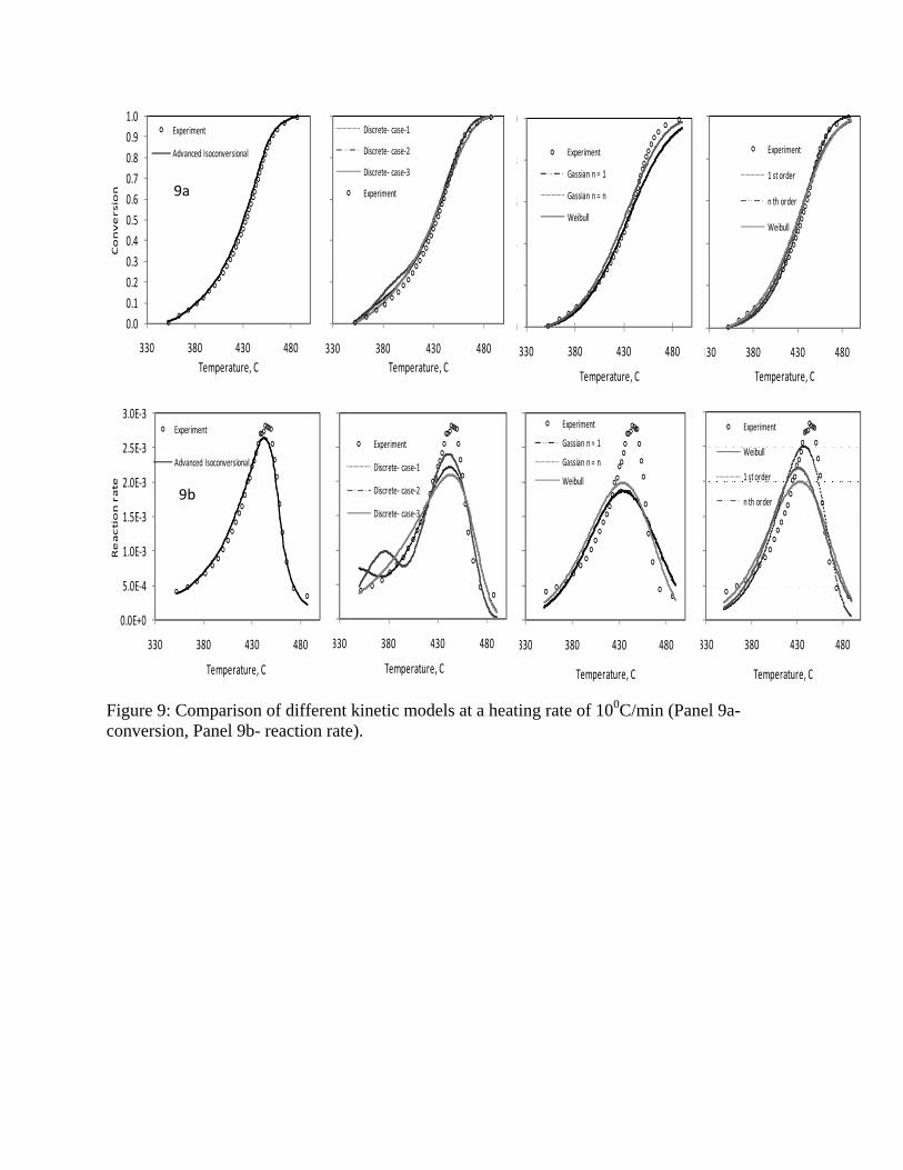
The reconstruction of conversion and rate experimental data using different Kinetic05 models and
Isokin were compared at all experimental heating rates. The results are shown for a heating rate of
100C/min in Figure 9. The general trend is that the cumulative conversions are matched reasonably
well while the rates have higher discrepancies.
Comparison of the Different Kinetic Models Used

14
The comparison of the sum of the root mean square (RMS) errors (all 7 experimental heating rates)
is shown in Figure 10 (10a- for reaction rates and 10b- for conversions). The errors were calculated
for 100 points of conversion at the same values of experimental temperatures. The RMS values are
lower for the advanced isoconversional method compared to the parameter fitting and reactivity
distribution models. The isoconversional approach from Kinetics05 also produced RMS values
comparable to the ones shown for the advanced isoconversional method. The parameter fitting
approaches, particular with discrete activation energies also result in reasonable RMS values. The
parameter fitting approaches may result in determination of parameter sets that are non-unique. For
example, the first order and nth order models with Gaussian distribution are characterized by
different parameter sets (Table 3), but produce about the same goodness of fit (Figure 10). When
this happens, model discrimination becomes an issue. However, these models are flexible, and can
be used with any reaction combinations (parallel, series, etc.). The isoconversion approach which
does not consider a kinetic model apriori gets around this, but may not be as flexible as the
parameter fitting methods. Burnham and Dinh (2007)49 argue that isocovension models are not
suitable for modeling reactions in series.
The kinetic parameters obtained from different models were used to extrapolate the data outside of
the experimental range. The resulting profiles are compared in Figure 11 for conversion and
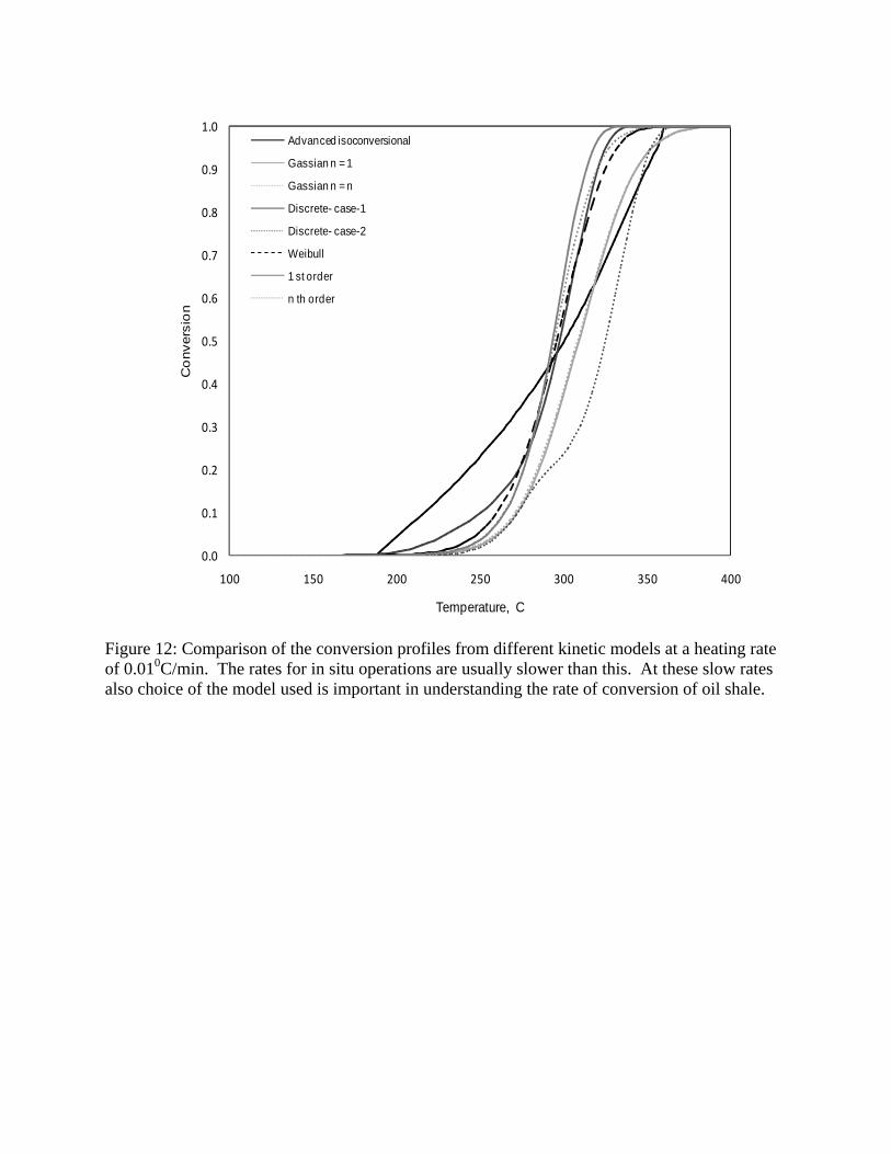
reaction rate at a heating rate of 1000C/min. Conversion profiles are also shown in Figure 12 for a
heating rate of 0.010C/min. The high heating rates would be applicable for a flash pyrolysis
process, while the slow heating rates are likely in in-situ heating of oil shale deposits. These
figures show that there are discernible consequences when the models are used to extrapolate the
data. At high heating rates, decomposition begins at much higher temperatures when the
isoconversional model is used. This trend is consistent with what is observed in the TGA. The

15
peak rates and the temperature range over which the reactions occur (spread of the rate curve) are
better reproduced when the isoconversion method is used. Similarly, at lower heating rates,
conversion begins at a lower temperature when the isoconversional model is used. The better
performance of the isoconversion model is attributed to the fact that it follows the progress of
reactions on the relevant conversion intervals.
Conclusions
In this paper, we present a thermogravimetric analysis data of oil shale pyrolysis at seven different
heating rates. Derivatives of the weight loss curves show a single major peak in the organic
weight loss region indicating that the decomposition is governed by single global mechanism.
Kinetic methods found suitable for the analysis of reactions of complex materials were used to
analyze the data and derive kinetic parameters. The advanced isoconversional method yielded
activation energies as function of conversion in the range of 93 kJ/mol to 245 kJ/mol. The
decomposition process can be viewed as consisting of multiple parallel reactions with individual
activation energies. Maximum uncertainties in activation energies computed using the advanced
isoconversion method were about 10% of the energy values calculated. Kinetic parameters were
also derived for a few other selected models using parameter fitting programs. The RMS errors
between the experimental and model values for the different approaches were compared. The
isoconversion approach produced the lowest RMS values in both rates and cumulative conversion
(for all of the heating rates, combined), but the parameter fitting approaches also produced
reasonable duplication of the data. The parameter fitting approaches using power law, activation
energy distribution or discrete energy values in specific conversion intervals are intuitive and fast.
However, model selection is difficult because numerous models produce equivalent results.
Change in one parameter (for example order) is compensated by changes in activation energies or

16
pre-exponential factors to produce comparable RMS values. Isoconversion models are in theory
“kinetic model” free and their applicability to the decomposition of a complex material like
kerogen is excellent. However, their applicability in reproducing multi-step kinetics has been
questioned. Application of these models to real life processes requires extending these models
outside of the experimental data range from which they were derived. It is shown that the choice
of the right model is of great consequence since model predictions outside of the experimental
range vary considerably between the models chosen. Even though this analysis has been conducted
with oil shale, the approach and conclusions are likely to be applicable to other complex materials.
Nomenclature
A = Frequency (pre-exponential) factor (min-1)
E = Activation energy (kJmol-1)
Eα = Activation energy at conversion α
ƒ (α) = Reaction model
ƒ (T) = Temperature dependency of the reaction rate
I = Integral symbol
N= Number of heating rates
R = Gas constant (8.314 kJmol -1 K-1)
T = Temperature (K)
T0 = Initial temperature
Tm = Temperature when reaction rate is maximum
Tα = Temperature at conversion α
W0 = Initial weight of the sample (mg)
Wt = Weight of the sample at time, t (mg)
W∞ = Weight of the sample at the end of the experiment (mg)

17
α = Conversion
β = Constant heating rate (oC/min)
Acknowledgements
The authors would like to acknowledge financial support from the U.S. Department of Energy,
National Energy Technology Laboratory – Grant Number: DE-FE0001243. The samples were
provided by Utah Geological Survey. The authors would like to thank Professor Wight for
providing the Isokin Software developed at the University of Utah for use. We would also like to
thank Dr. Burnham of American Shale Oil Company for providing key papers and insight to the
kinetic models through various discussions.
References
1. Smith JW. Oil shale resources of the United States. CSM Mineral and Energy Resources
Series. 1980;23(6).
2. Dyni JR. Geology and resources of some world oil shale deposits. Oil Shale.
2003;20(3):193-252.
3. Bartis JT, LaTourrette T, Dixon L, Peterson DJ, Cecchine G. OIl shale development in the
United States- Prospective and policy issues2005.
4. VandenBerg MD. Basin-wide evaluation of the uppermost green river formation's oil-shale
resource, Unita Basin, Utah and Colorado: Utah Geological Survey;2008.
5. Nuttall HE, Guo T, Schrader S, Thakur DS. Pyrolysis kinetics of several key world oil
shales. In: Miknis FP, McKay JF, eds. Geochemistry and chemistry of oil shales. Vol 230:
American Chemical Society; 1983:269-300.

18
6. Burham AK, Richardson JH, Coburn TT. Pyrolysis kinetics for western and eastern oil
shale. Paper presented at: In proceedings of the 17th intersociety energy conversion
engineering conference1982; New York.
7. Torrente MC, Galan MA. Kinetics of the thermal decomposition of oil shale from
puertollano (Spain). Fuel. 2001;80(3):327-334.
8. Burnham AK. Oil evolution from a self-purging reactor: Kinetic and composition at
2C/min and 2 C/h. Energy Fuels. 1991;5(1):205-214.
9. Charlesworth JM. Oil shale pyrolysis: 1. Time and temperature dependence of product
composition. Ind. Eng. Chem. Process Des. Dev. 1985;24(4):1117-1125.
10. Burnham AK, Singleton MF. High-pressure pyrolysis of green river oil shale. In: Miknis
FP, McKay JF, eds. Geochemistry and chemistry of oil shales1983:335-351.
11. Sohn HY, Yang HS. Effect of reduced pressure on oil shale retorting. 1. Kinetics of oil
generation. Ind. Eng. Chem. Process Des. Dev. 1985;24(2):265-270.
12. Yang HS, Sohn HY. Mathematical analysis of the effect of retorting pressure on oil yield
and rate of oil generation from oil shale. Ind. Eng. Chem. Process Des. Dev.
1985;24(2):274-280.
13. Stainforth JG. Practical kinetic modeling of petroleum generation and expulsion. Mar.
Petrol. Geol. 2009;26(4):552-572.
14. Burnham AK, Happe JA. On the mechanism of kerogen pyrolysis. Fuel. 1983;63(10):1353-
1356.
15. Burnham AK. Relationship between hydrous and ordinary pyrolysis. Paper presented at:
NATO advanced study institute on composition, geochemistry and conversion of oil shales
conference Akcay, Turkey1995

19
16. Pan C, Geng A, Zhong N, Liu J, Yu L. Kerogen pyrolysis in the presence and absence of
water and minerals. 1. Gas components. Energy Fuels. 2008;22(1):416-427.
17. Lewan MD, Ruble TE. Comparison of petroleum generation kinetics by isothermal
hydrous and non-isothermal open system pyrolysis. Org. Geochem. 2002;33(12):1457-
1475.
18. Michels R, Landaisa P, Torkelsonb BE, Philpc RP. Effects of effluents and water pressure
on oil generation during confined pyrolysis and high-pressure hydrous pyrolysis. Geochim.
Cosmochim. Acta. 1995;59(8):1589-1604.
19. Hill GR, Johnson DJ, Miller L, Dougan JL. Direct production of low pour point high
gravity shale oil. Ind. Eng. Chem. Prod. Res. Dev. 1967;6(1):52-59.
20. Haung ETS. Retorting of single oil shale blocks with nitrogen and air. Soc. Petrol. Eng. J.
1977;17(5):331-336.
21. Jaber JO, Probert SD. Non-isothermal thermogravimetry and decomposition kinetics of two
Jordian oil shales under different processing conditions. Fuel Process.Technol.
2000;63(1):57-70.
22. Kavianian HR, Yesavage VF, Dickson PF, Peters RW. Kinetic simulation model for steam
pyrolysis of oil shale feedstock. Ind. Eng. Chem. Res. 1990;29(4):527-534.
23. Fathoni AZ, Batts BD. A literature review of fuel stability studies with a particular
emphasis on shale oil. Energy Fuels. 1992;6(6):681–693.
24. A technical, economical and legal assesment of North maerican heavy oil, oil sands, and
oil shale resources; In responce to energy policy Act of 2005 section 369(p); Prepared by
Utah heavy oil program 2007.

20
25. Rajeshwar K. The kinetics of the thermal decomposition of green river oil shale kerogen by
non-Isothermal thermogravimetry. Thermochim. Acta. 1981;45(3):253-263.
26. Galan MA, Smith JM. Pyrolysis of oil shale: Experimental study of transport effects.
AIChE J. 1983;29(4):604-610.
27. Hillier J, Fletcher J, Orgill J, Isackson C, Fletcher TH. An Improved method for
determination of kinetic parameters from constant heating rate TGA oil shale pyrolysis
data. Prep. Pap.-Am. Chem. Soc., Div. Fuel. Chem. 2009;54(1):155-157.
28. Li S, Yue C. Study of pyrolysis kinetics of oil shale. Fuel. 2003;82(3):337-342.
29. Li S, Yue C. Study of different kinetic models for oil shale pyrolysis. Fuel
Process.Technol. 2003;85(1):51-61.
30. Qing W, Baizhong S, Aijuan H, Jingru B, Shaohua L. Pyrolysis charactristic of huadian oil
shale. Oil Shale. 2007;24(2):147-157.
31. William PT, Ahmad N. Influence of process conditions on the pyrolysis of Pakistani oil
shale. Fuel. 1999;78(6):653-662.
32. Thakur DS, Nuttal HE. Kinetics of pyrolysis of Moroccan oil shale by thermogravimetry.
Ind. Eng. Chem. Process Des. Dev. 1987;26(7):1351-1356.
33. Shin SM, Sohn HY. Nonisothermal determination of the intrinsic kinetics of oil generation
from oil shale. Ind. Eng. Chem. Process Des. Dev. 1980;19(3):420-426.
34. Campbell JH, Koskinas GH, D SN. Kinetics of oil generation from Colorado oil shale Fuel.
1978;57(6):372-376.
35. Hubbard AB, Robinson WE. A thermal decomposition study of Colorado oil shale: U.S.
Bureau of Mine:Report of investigation #4744;1954.

21
36. Leavitt DR, Tyler AL, Kafesjiant AS. Kerogen decomposition kinetics of selected green
river and eastern U.S. oil shales from thermal solution experiments. Energy Fuels.
1987;1(6):520-525.
37. Allred VD. Kinetics of oil shale pyrolysis. Chem. Eng. Prog. 1966;62(8):55-60.
38. Braun RL, Rothman AJ. Oil shale pyrolysis: Kinetics and mechanism of oil production.
Fuel. 1975;54(2):129-131.
39. Burnham AK. Chemistry and kinetics of oil shale retorting. Oil shale: A solution to the
liquid fuel dilemma. Vol 103: ACS symposium series; 2010:115–134.
40. Braun RL, Burnham AK. Analysis of chemical reaction kinetics using a distribution of
activation energies and simpler models. Energy Fuels. 1987;1:153-161.
41. Burnham AK, Braun RL. General kinetic model of oil shale pyrolysis. In Situ. 1985;9(1):1-
23.
42. Burnham AK, Braun RL, Coburn TT, Sandvik EI, Curry DJ, Schmidt BJ, Noble RA. An
appropriate kinetic model for well-preserved algal kerogen. Energy Fuels. 1996;10(6):49-
59.
43. Brown ME, Maciejewski M, Vyazovkin S, Nomen R, Sempere J, Burnham A, Opfermann
J, Strey R, Anderson HL, Kemmeler A, Janssens J, Desseyn HO, Li CR, Tang TB, Roduit
B, Malek J, Mitsuhasshi T. Computational aspects of kinetic analysis: Part A: - The ICTAC
kinetics project-data, methods and results. Thermochim. Acta. 2000;355:125-143.
44. Burnham AK. Computaional aspects of kinetic analysis. Part D: The ICTAC kinetic project
- Multi-thermal-history model fitting methods and their relation to isoconversion methods
Thermochim. Acta. Vol 3552000:165-170.

22
45. Maciejewski M. Computational aspects of kinetic analysis: Part B- The ICTAC project- the
decomposition kinetics of calcium carbonate revisited, or some tips on survival in the
kinetic minefield. Thermochim. Acta. 2000;355:125-143.
46. Roudit B. Computational aspects of kinetic analysis: Part E- Numerical techniques and
kinetics of solid state processes. Thermochim. Acta. 2000;35:171-180.
47. Vyazovkin S. Computational aspects of kinetic analysis: Part C- The ICTAC project- The
light at the end of the tunnel?. Thermochim. Acta. 2000;355:155-163.
48. Burnham AK, Braun RL. Global kinetic analysis of complex materials. Energy Fuels.
1999;13(1):1–22.
49. Burnham AK, Dinh LN. A comparision of isoconversional and model-fitting kinetic
parameter estimation and application predictions. J. Therm. Anal. Calorim.
2007;89(2):479-490.
50. Starink MJ. The determination of activation energy from linear heating rate experiments: A
comparison of the accuracy of isoconversion methods. Thermochim. Acta. 2003;404:163-
176.
51. Sundararaman P, Merz PH, Mann RG. Determination of kerogen activation energy
distribution. Energy Fuels. 1992;6(6):793-803.
52. Al-Ayed OS, Matouq M, Anbar Z, Khaleel AM, Abu-Nameh E. Oil shale pyrolysis
kinetics and variable activation energy principle. Appl. Energ. 2010;87(4):1269-1272.
53. Friedman HL. Kinetics of thermal degradation of charforming plastics from
thermogravimetry. In: Application to a phenolic plastic. J. Polym. Sci.Part C.
1964;6(1):183–195.

23
54. Vyazovkin S, Wight CA. Estimating realistic confidence intervals for the activation energy
determined from thermoanalytical measurements. Anal. Chem. 2000;72(14):3171-3175.
55. Vyazovkin S, Wight CA. Isothermal and non-isothermal kinetics of thermally stimulated
reactions of solids. Int. Rev. Phys. Chem. 1998;17(3):407-433.
56. Vyzovkin SV, Lesnikovich AL. Practical application of isoconversional methods.
Thermochim. Acta. 1992;203:177-185.
57. Vyazovkin S, Wight CA. Kinetics in solids. Annu. Rev. Phys. Chem. 1997;48:125-149.
58. Hutton A, Bharati S, Robl T. Chemical and petrographical classification of
kerogen/macerals. Energy Fules. 1994;8(6):1478-1488.
59. Behar F, Vandenbroucke M. Chemical modelling of kerogens. Org. Geochem.
1987;11(1):15-24.
60. Vandenbroucke M, Largeau C. Kerogen origin, evaluation and structure. Org. Geochem.
2007;38:719-833.
61. Blazek A. Thermal analysis. In: Tyson JF, ed. Thermal analysis: Van Nostrand Reinhold,
London; 1973.
62. Vyazovkin S, A LL. Estimation of the pre-exponential factor in the isoconversional
calculation of effective kinetic parameters. Thermochimica Acta. 1988;128:297-300.
63. Vyazovkin S, Linert W. Detecting isokinetic relationships in non-isothermal systems by the
isoconversional method Thermochim. Acta. 1995;269/270:61-72.
64. Vyazovkin S, Sbirrazzuoli N. Confidence intervals for the activation energy estimated by
few experiments. Anal. Chim. Acta. 1997;355:175-180.
65. Doyle CD. Estimating isothermal life from thermogravimetric data. J. Appl. Polym. Sci.
1962;6(24):639-642.

24
66. Senum GI, Yang RT. Rational approximations of the integral of the Arrhenius function. J.
Therm. Anal. Calorim. 1977;11(3):445-447.
67. Vyazovkin S. Reply to “What is meant by the term ‘variable activation energy’ when
applied in the kinetics analyses of solid state decompositions (crystolysis reactions)?”
Thermochim Acta. 2003;397(1-2):269-271.
68. Constable FH. The mechanism of catalytic decomposition. Proceedings of the Royal
Society of London. Vol 108: The Royal Society; 1923:355-378.
69. Charlesworth JM. Oil Shale Pyrolysis. 2. Kinetics and mechanism of Hydrocarbon
Evolution. Ind. Eng. Chem. Process Des. Dev. 1985;24:1125-1132.
70. Boudreau BP, Ruddick BR. On a reactive continuum representation of organic matter
diagenesis. Am. J. Sci. 1991;291:507-538.
71. Burnham AK, Braun RL, Gregg HR. Comparison of methods for measuring kerogen
pyrolysis rates and fitting kinetic parameters. Energy Fuels. 1987;1(6):452-458.
72. Lakshmanan CC, White N. A new distributed activation-energy model using weibull
distribution for the representation of complex kinetics. Energy Fuels. 1994;8(6):1158-
1167.

Table 1. Elemental analysis of the Green River oil shale. Ten samples were analyzed and
the mean and standard deviation are shown.
Oil Shale Sample Mean % Stdev
Carbon 17.45 0.26 Hydrogen 1.6 0.08 Nitrogen 0.53 0.06 Sulfur 0.18 0.04 Oxygen 15.69 0.79 H/C % (molar) 1.1 O/C % (molar) 0.67

Table 2. Analysis criteria for the non-isothermal TGA pyrolysis data.
Heating rate
Initial weight
Analysis Criteria Start End Maximum
β mg T 0C
wt % Loss
T 0C
wt % Loss
Tmax, 0C
wt % Loss
0.5 22.64 255.6 1.32 421.6 8.02 392.7 6.48 1 28.64 269.6 1.16 437.6 7.48 398.3 5.79 2 26.90 280.0 1.33 456.4 8.43 414.1 6.52 5 25.97 348.9 2.17 474 9.41 432.2 7.17 10 38.45 349.7 1.74 490 9.67 445.6 7.26 20 29.49 371.6 1.58 504 10.68 460.1 7.92 50 22.37 377.3 1.43 530.6 11.13 477.0 7.89

Table 3. Parameters obtained using selected kinetic models available in Kinetic05.
Kinetic models
E (kJ/mol)
A (1/s) Order Paremeter-
1 Paremeter-
2
Gaussian n = n 180.061 8.12E+10 0.53 4.19E+00 n = 1 181.446 1.29E+11 1.00 3.78E+00
Discrete Case-1 Fig 8-(a) 5.72E+09 1.00 Case-2 Fig8-(b) 1.00E+14 1.00 Case-3 Fig8-( c) e(a+bE) 1.00
Weibull 163.154 6.64E+09 1.00 1.04E+04 9.99E+00 1st order 156.968 2.19E+09 1.00 nth order 160.735 5.80E+09 1.65 1.65
Isoconversional Figure-4 1 Friedman based

Figure 1: Non-isothermal TGA pyrolysis thermograms: rates go from 0.50C/min to 500C/min. The solid lines are weight loss curves and the dashed lines are derivatives. The arrow indicates that the rates increase as we go from bottom to the top. In the derivative curves, the highest peaks for the highest rate used. The second set of derivative peaks is due to mineral decomposition.

0
50
100
150
200
250
300
0 0.2 0.4 0.6 0.8 1
Five heating rates- (0.5-1-10-20-50C/min)
5 (0.5-1-10-20-50)
0
50
100
150
200
250
300
0 0.2 0.4 0.6 0.8 1
Five heating rates- (0.5.-5-10-20-50C/min)
5 (0.5.-5-10-20-50)
0
50
100
150
200
250
300
0 0.2 0.4 0.6 0.8 1
Three heating rates- (1-5-20C/min)
3 (1-5-20)
0
50
100
150
200
250
300
0 0.2 0.4 0.6 0.8 1
Three heating rates- (10-20-50C/min)
3 (10-20-50)
Figure 2: Distribution of activation energies for pyrolysis of Green River oil shale calculated using the advanced isoconversional method. The uncertainties in activation energy values are shown for different numbers of heating rates considered and for different combinations. As all of the heating rates are used, uncertainties are reduced over the entire conversion range (2d). The final calculation of activation energies with uncertainties are shown in Figure 3.
a b
c d

0.E+00
1.E+14
2.E+14
3.E+14
4.E+14
5.E+14
6.E+14
7.E+14
8.E+14
9.E+14
1.E+15
0 0.1 0.2 0.3 0.4 0.5 0.6 0.7 0.8 0.9 1
A.f(α)
, 1/s
Extent of conversion
Distribution of A.f(α)
0
50
100
150
200
250
300
0 0.1 0.2 0.3 0.4 0.5 0.6 0.7 0.8 0.9 1
Act
ivat
ion
en
ergy
, kJ/
mol
Extent of conversion
Distribution of activation energy
Figure 3: Distribution of kinetic parameters with extent of conversion (3a- Activation energy, 3b-A·f(α)) determined using the advanced isoconversional method. All of the seven rates were used in calculating the kinetic parameters. Uncertainties in activation energy values are also shown.
3a
3b

0
50
100
150
200
250
300
0 0.1 0.2 0.3 0.4 0.5 0.6 0.7 0.8 0.9 1
Activatio
n e
nerg
y a
nd
ln(A
)
Conversion
Advanced Isoconversional_E
Friedman_E
Advanced Isoconversiona_ln(A)
Friedman_ln(A)
Figure 4: Comparison of kinetic parameters from advanced isoconversional and the Friedman method. The kinetic model is assumed to be first-order for this comparison.

Isokin ‐ y = 0.171x ‐ 1.477, R2 = 0.995
Friedman‐ y = 0.170x ‐ 1.489, R2 = 0.999
0
5
10
15
20
25
30
35
40
45
80 100 120 140 160 180 200 220 240 260
Lo
garith
mic
of
pre
-exp
onential f
acto
r (A
)
Activation energy (E), kJ/mol
Advanced Isoconversional
Friedman
Linear (Advanced Isoconversional)
Linear (Friedman)
Figure 5: Constable plots for Friedman and advanced isoconversional kinetic parameters.

0
0.1
0.2
0.3
0.4
0.5
0.6
0.7
0.8
0.9
1
200 250 300 350 400 450 500 550
Norm
alize
d co
nver
sion
Temperature, oC
Expt-0.5C/min
Simul-0.5C/min
Expt-1C/min
Simul-1C/min
Expt-2C/min
Simul-2C/min
Expt-5C/min
Simul-5C/min
Expt-10C/min
Simul-10C/min
Expt-20C/min
Simul-20C/min
Expt-50C/min
Simul-50C/min
Figure 6: Experimental and simulated conversion profiles at different heating rates using the advanced isoconversional method. MATLAB-based computational method described in the text was used.

0
0.1
0.2
0.3
0.4
0.5
0.6
0.7
0.8
0.9
1
100 200 300 400 500 600
Conv
ersi
on
Temperature, oC
Simul-0.01C/min
Simul-0.01C/min
Simul-0.1C/min
Simul-0.1C/min
Simul-10C/min
Simul-10C/min
Simul-100C/min
Simul-100C/min
Simul-500C/min
Simul-500C/min
Figure 7: Simulated conversion profiles at extrapolated constant heating rates using two different initial temperatures. Continuous lines show profiles with T0 = 1000C and dotted lines depict extrapolations with T0 calculated from equation 8.

0
10
20
30
40
50
60
26
93
160
228
295
362
429
496
564
631
698
765
832
Perc
ent
Activation energy, kJ/mol
Discrete- Case-3, A = 0.00E00
0
10
20
30
40
50
60
70
198
200
202
204
206
208
210
212
214
216
218
220
222
Perc
ent
Activation energy, kJ/mol
Discrete- Case- 2, A = 1.0E14 S-1
0
10
20
30
40
50
60
70
80
90
140
142
144
146
148
150
152
154
156
158
160
162
164
Perc
ent
Activation energy, kJ/mol
Discrete- Case-1, A = 5.73E09 S-1
Figure 8: Distribution of activation energies from discrete reactivity models (Cases 1-3 as described in the text).
0.0
0.2
0.4
0.6
0.8
1.0
330 380 430 480
Conversion
Temperature, C
Experiment
1 st order
n th order
Weibull
0.0
0.2
0.4
0.6
0.8
1.0
330 380 430 480
Conversion
Temperature, C
Experiment
Gassian n = 1
Gassian n = n
Weibull
0.0
0.2
0.4
0.6
0.8
1.0
330 380 430 480
Temperature, C
Discrete‐ case‐1
Discrete‐ case‐2
Discrete‐ case‐3
Experiment
0.0
0.1
0.2
0.3
0.4
0.5
0.6
0.7
0.8
0.9
1.0
330 380 430 480
Conversion
Temperature, C
Experiment
Advanced Isoconversional
0.0E+0
5.0E‐4
1.0E‐3
1.5E‐3
2.0E‐3
2.5E‐3
3.0E‐3
330 380 430 480
Temperature, C
Experiment
Weibull
1 st order
n th order
0.0E+0
5.0E‐4
1.0E‐3
1.5E‐3
2.0E‐3
2.5E‐3
3.0E‐3
330 380 430 480
Temperature, C
Experiment
Gassian n = 1
Gassian n = n
Weibull
0.0E+0
5.0E‐4
1.0E‐3
1.5E‐3
2.0E‐3
2.5E‐3
3.0E‐3
330 380 430 480
Temperature, C
Experiment
Discrete‐ case‐1
Discrete‐ case‐2
Discrete‐ case‐3
0.0E+0
5.0E‐4
1.0E‐3
1.5E‐3
2.0E‐3
2.5E‐3
3.0E‐3
330 380 430 480
Reaction rate
Temperature, C
Experiment
Advanced Isoconversional
Figure 9: Comparison of different kinetic models at a heating rate of 100C/min (Panel 9a- conversion, Panel 9b- reaction rate).
9a
9b

0.0E+0
1.0E‐1
2.0E‐1
3.0E‐1
4.0E‐1
5.0E‐1
6.0E‐1
Conversion-Sum of RMS
Conversion
0.0E+0
1.0E‐3
2.0E‐3
3.0E‐3
4.0E‐3
5.0E‐3
6.0E‐3
7.0E‐3Rate- Sum of RMS
Reaction rate
Figure 10: Comparison of different kinetic models based on sum of RMS (root mean square) residues. In all these calculations, 100 experimental data points were used. RMS is summed over all of the seven experimental heating rates.
10a 10b

0.0
0.1
0.2
0.3
0.4
0.5
0.6
0.7
0.8
0.9
1.0
350 400 450 500 550 600 650
Co
nvers
ion
Temperature, C
Advanced isoconversional
Gassian n = 1
Gassian n = n
Discrete- case-1
Discrete- case-2
Weibull
1 st order
n th order
0.0E+00
1.0E‐02
2.0E‐02
3.0E‐02
4.0E‐02
5.0E‐02
6.0E‐02
300 350 400 450 500 550 600R
eactio
n rate
Temperature, C
Advanced Isoconversional
Gassian n = 1
Gassian n = n
Discrete- case-1
Discrete- case-2
Weibull
1 st order
n th order
Figure 11: Comparison of different kinetic models at a heating rate of 1000C/min (11a- conversion, 11b- reaction rate). It is seen that under fast pyrolysis conditions, model of choice does have significant impact on predictions.
11a 11b
0.0
0.1
0.2
0.3
0.4
0.5
0.6
0.7
0.8
0.9
1.0
100 150 200 250 300 350 400
Co
nvers
ion
Temperature, C
Advanced isoconversional
Gassian n = 1
Gassian n = n
Discrete- case-1
Discrete- case-2
Weibull
1 st order
n th order
Figure 12: Comparison of the conversion profiles from different kinetic models at a heating rate of 0.010C/min. The rates for in situ operations are usually slower than this. At these slow rates also choice of the model used is important in understanding the rate of conversion of oil shale.