desmond user manual - national cancer institute · pdf filedesmond 2.2 user manual 1 desmond...
TRANSCRIPT

Desmond User Manual
Desmond 2.2
User Manual
Schrödinger Press

Desmond User Manual Copyright © 2009 Schrödinger, LLC. All rights reserved.
While care has been taken in the preparation of this publication, Schrödinger
assumes no responsibility for errors or omissions, or for damages resulting from
the use of the information contained herein.
Canvas, CombiGlide, ConfGen, Epik, Glide, Impact, Jaguar, Liaison, LigPrep,
Maestro, Phase, Prime, PrimeX, QikProp, QikFit, QikSim, QSite, SiteMap, Strike, and
WaterMap are trademarks of Schrödinger, LLC. Schrödinger and MacroModel are
registered trademarks of Schrödinger, LLC. MCPRO is a trademark of William L.
Jorgensen. Desmond is a trademark of D. E. Shaw Research. Desmond is used with
the permission of D. E. Shaw Research. All rights reserved. This publication may
contain the trademarks of other companies.
Schrödinger software includes software and libraries provided by third parties. For
details of the copyrights, and terms and conditions associated with such included
third party software, see the Legal Notices for Third-Party Software in your product
installation at $SCHRODINGER/docs/html/third_party_legal.html (Linux OS) or
%SCHRODINGER%\docs\html\third_party_legal.html (Windows OS).
This publication may refer to other third party software not included in or with
Schrödinger software ("such other third party software"), and provide links to third
party Web sites ("linked sites"). References to such other third party software or
linked sites do not constitute an endorsement by Schrödinger, LLC. Use of such
other third party software and linked sites may be subject to third party license
agreements and fees. Schrödinger, LLC and its affiliates have no responsibility or
liability, directly or indirectly, for such other third party software and linked sites,
or for damage resulting from the use thereof. Any warranties that we make
regarding Schrödinger products and services do not apply to such other third party
software or linked sites, or to the interaction between, or interoperability of,
Schrödinger products and services and such other third party software.
June 2009

Contents
Document Conventions ..................................................................................................... ix
Chapter 1: Introduction ....................................................................................................... 1
1.1 Installation and Configuration ................................................................................ 2
1.2 The Maestro Interface to Desmond ........................................................................ 3
1.3 Desmond Calculations Overview ........................................................................... 4
1.4 Citing Desmond in Publications ............................................................................. 5
Chapter 2: Building a Model System ........................................................................ 7
2.1 Adding Solvent .......................................................................................................... 7
2.2 Setting Up the Boundary Box ................................................................................. 8
2.3 Adding a Membrane .................................................................................................. 9
2.4 Using Custom Charges .......................................................................................... 11
2.5 Adding Ions .............................................................................................................. 11
2.5.1 Defining an Excluded Region............................................................................ 12
2.5.2 Ion Placement ................................................................................................... 12
2.5.3 Adding a Salt..................................................................................................... 14
2.6 Running the Job ...................................................................................................... 14
2.7 Quick Setup Instructions ....................................................................................... 14
Chapter 3: Running a Desmond Simulation from Maestro...................... 17
3.1 Overview of the General Desmond Panels ......................................................... 17
3.2 Selecting a Model System ..................................................................................... 18
3.3 Minimizations ........................................................................................................... 19
3.4 Molecular Dynamics Simulations......................................................................... 20
3.5 Simulated Annealing Simulations ........................................................................ 22
3.6 Replica Exchange Simulations ............................................................................. 24
3.7 Simulations on Systems with Membranes ......................................................... 26
Desmond 2.2 User Manual iii

Contents
iv
3.8 Setting Options for Desmond Simulations......................................................... 27
3.8.1 The Integration Tab ........................................................................................... 28
3.8.2 The Ensemble Tab ............................................................................................ 29
3.8.3 The Minimization Tab ........................................................................................ 31
3.8.4 The Interaction Tab ........................................................................................... 32
3.8.5 The Restraints Tab............................................................................................ 33
3.8.6 The Output Tab ................................................................................................. 33
3.8.7 The Misc Tab..................................................................................................... 35
3.9 Running a Simulation Job ..................................................................................... 36
Chapter 4: Running FEP Simulations .................................................................... 39
4.1 FEP Panels................................................................................................................ 39
4.2 Ligand Functional Group Mutation ...................................................................... 40
4.3 Ring Atom Mutation ................................................................................................ 42
4.4 Protein Residue Mutation ...................................................................................... 44
4.5 Total Solvation Free Energy Calculation............................................................. 46
4.6 Selecting the Environment and FEP Protocol.................................................... 47
4.7 FEP Results .............................................................................................................. 49
4.7.1 Relative Free-Energy Differences ..................................................................... 49
4.7.2 Total Solvation Free Energies ........................................................................... 49
4.8 Customizing and Restarting FEP Simulations .................................................. 50
Chapter 5: Analyzing Simulations ............................................................................. 53
5.1 Viewing Trajectories ............................................................................................... 53
5.2 Simulation Quality Analysis .................................................................................. 56
Desmond 2.2 User Manual

Contents
Chapter 6: Running Desmond Simulations from the CommandLine ......................................................................................................................................... 59
6.1 The desmond Command........................................................................................ 59
6.2 Running Multiple Simulations............................................................................... 62
6.2.1 Examples of Running MultiSim ......................................................................... 64
6.2.2 Sample MultiSim Job (.msj) File ....................................................................... 64
6.2.3 Treatment of Intermediate Files ........................................................................ 67
6.3 Building a Model System ....................................................................................... 67
6.3.1 Reading the Structures .................................................................................... 68
6.3.2 Adding a Membrane......................................................................................... 70
6.3.3 Setting the Box Shape and Dimensions............................................................ 70
6.3.4 Setting Force Field Information ......................................................................... 71
6.3.5 Setting the Number and Location of Ions.......................................................... 71
6.3.6 Solvating the System ....................................................................................... 72
6.3.7 Writing the Output File ...................................................................................... 72
Chapter 7: Using VMD for Desmond Trajectories .......................................... 73
7.1 Installing VMD and the Desmond Plugin ............................................................ 73
7.2 Reading a CMS File and a Desmond Trajectory ............................................... 75
7.3 Writing a Maestro File............................................................................................. 76
Chapter 8: Using Alternate Force Field Parameters andConstraints......................................................................................................................... 77
8.1 The viparr Utility ...................................................................................................... 77
8.2 The build_constraints Utility ................................................................................. 79
8.3 Input and Output Files............................................................................................ 80
8.4 Specifying Multiple Force Fields .......................................................................... 81
8.5 User-Defined Force Fields ..................................................................................... 82
8.6 Known Issues........................................................................................................... 83
Desmond 2.2 User Manual v

Contents
vi
Chapter 9: Utilities................................................................................................................ 85
9.1 solvate_pocket ......................................................................................................... 85
9.1.1 Methodology ..................................................................................................... 85
9.1.2 Command Syntax ............................................................................................. 86
9.1.3 Command File Syntax....................................................................................... 86
9.2 manipulate_trj.py..................................................................................................... 89
9.3 amber_prm2cms.py ................................................................................................ 90
9.4 mold_gpcr_membrane.py ...................................................................................... 90
Appendix A: Creating a CMS File from a Full System Maestro File . 93
Appendix B: The multisim Utility................................................................................. 95
B.1 Running multisim .................................................................................................. 95
B.1.1 Template multisim Commands.......................................................................... 95
B.1.2 Node Locking.................................................................................................... 96
B.1.3 Restarting multisim Jobs .................................................................................. 96
B.1.4 Obtaining Information from multisim Checkpoint Files ..................................... 97
B.2 The multisim File Syntax ...................................................................................... 98
B.2.1 General Keywords .......................................................................................... 100
B.2.2 Desmond-Specific Common Keywords .......................................................... 100
B.2.3 The restrain Keyword...................................................................................... 101
B.2.4 The atom_group Keyword............................................................................... 102
B.2.5 The task Stage ............................................................................................... 103
B.2.6 The system_builder Stage.............................................................................. 103
B.2.7 The simulate and replica_exchange Stages................................................... 104
B.2.8 The minimize Stage........................................................................................ 105
B.2.9 The solvate_pocket Stage .............................................................................. 106
B.2.10 The extern Stage .......................................................................................... 107
B.2.11 The fep_analysis Stage ................................................................................ 109
Desmond 2.2 User Manual
Contents
Appendix C: The Desmond Configuration File .............................................. 111
C.1 General Structure ................................................................................................ 111
C.2 Units ....................................................................................................................... 112
C.3 Configuration File Sections ............................................................................... 112
C.3.1 The boot Section ............................................................................................ 113
C.3.2 The constraint Section.................................................................................... 113
C.3.3 The Desmond Section.................................................................................... 113
C.3.4 The force Section ........................................................................................... 114
C.3.5 The global_cell Section .................................................................................. 116
C.3.6 The integrator Section .................................................................................... 117
C.3.7 The mdsim Section......................................................................................... 120
C.3.8 The minimize Section ..................................................................................... 121
C.3.9 The remd Section ........................................................................................... 121
C.3.10 The vrun Section .......................................................................................... 122
C.4 Plugin Descriptions ............................................................................................. 122
C.5 Examples ............................................................................................................... 125
C.5.1 FEP Calculations............................................................................................ 125
C.5.2 Replica Exchange........................................................................................... 127
C.5.3 Simulated Annealing....................................................................................... 127
C.5.4 Instructing Desmond to Glue Close Solute Molecules Together .................... 127
Appendix D: Analyzing a Simulation from the Command Line ........... 129
D.1 simulation_block_data.py ................................................................................. 129
D.2 simulation_block_test.py .................................................................................. 130
D.3 Simulation Block Analysis (.sba) File Syntax ................................................. 130
D.4 Simulation Block Test (.sbt) File Syntax .......................................................... 131
References .............................................................................................................................. 133
Getting Help ........................................................................................................................... 137
Desmond 2.2 User Manual vii

viii
Desmond 2.2 User Manual
Document Conventions
In addition to the use of italics for names of documents, the font conventions that are used inthis document are summarized in the table below.
Links to other locations in the current document or to other PDF documents are colored likethis: Document Conventions.
In descriptions of command syntax, the following UNIX conventions are used: braces { }
enclose a choice of required items, square brackets [ ] enclose optional items, and the barsymbol | separates items in a list from which one item must be chosen. Lines of commandsyntax that wrap should be interpreted as a single command.
File name, path, and environment variable syntax is generally given with the UNIX conven-tions. To obtain the Windows conventions, replace the forward slash / with the backslash \ inpath or directory names, and replace the $ at the beginning of an environment variable with a% at each end. For example, $SCHRODINGER/maestro becomes %SCHRODINGER%\maestro.
In this document, to type text means to type the required text in the specified location, and toenter text means to type the required text, then press the ENTER key.
References to literature sources are given in square brackets, like this: [10].
Font Example Use
Sans serif Project Table Names of GUI features, such as panels, menus,menu items, buttons, and labels
Monospace $SCHRODINGER/maestro File names, directory names, commands, envi-ronment variables, and screen output
Italic filename Text that the user must replace with a value
Sans serifuppercase
CTRL+H Keyboard keys
Desmond 2.2 User Manual ix

x
Desmond 2.2 User Manual
Desmond User Manual
Chapter 1
Chapter 1: Introduction
Desmond is a new explicit-solvent molecular dynamics program developed by D. E. ShawResearch. Desmond was created from scratch with an emphasis on accuracy, speed and scal-ability. It supports many of the most sought-after features in a modern molecular dynamicsprogram, including:
• Highly scalable parallel execution
• Explicit solvent simulations with periodic boundary conditions using cubic, orthorhom-bic, and triclinic simulation boxes. Truncated octahedron and rhombic dodecahedron aresupported via their triclinic analogues.
• Support for isotropic, semi-isotropic and anisotropic pressure coupling
• Smooth particle mesh Ewald method for accurate and efficient evaluation of long-rangeelectrostatics
• NVE, NVT, NPT, NPAT, NPγT ensembles with Berendsen, Langevin, or Nosé-Hooverthermostats, and Berendsen, Langevin, or Martyna-Tobias-Klein barostats
• Symplectic integration of the equations of motion using a multiple time step approach,RESPA
• Elimination of many sources of numerical error, permitting accurate and fast calculationsusing single-precision arithmetic
• Accurate implementation of constraints to eliminate high-frequency motions and thuspermit larger time steps
• Exploitation of modern computer chip features to enhance speed (SIMD)
• Efficient calculation of the pressure
• Accurate checkpointing mechanism for continuing or restoring simulations
• Template-based support for widely-used force fields (using viparr).
• Viewing of trajectories with VMD using a Desmond plug-in.
A description of Desmond was published, along with performance data, as part of the confer-ence proceedings of the ACM/IEEE Conference on SuperComputing 2006 (SC06) [1]. Whiledeveloping Desmond, D. E. Shaw Research has introduced and extended a number of scientific
Desmond 2.2 User Manual 1

Chapter 1: Introduction
2
algorithms, including new parallelization strategies and numerical techniques, some of whichhave been published [2–5].
Problem-solving often involves using a wide range of modelling techniques, so integratingDesmond into Schrödinger’s premier molecular modelling suite for drug developmentenhances the utility of both. Examples of such synergies include:
• The Protein Preparation Wizard, LigPrep (ligand structure) and Epik (ligand protonationstate) preparation tools can be used to ensure that the structures provided to Desmond arechemically correct. Such careful system preparation often represents a crucial step priorto initiating a molecular dynamics simulation.
• Prime can be used to create homology models for use in simulations and to repair proteinstructures.
• Glide can be used to generate relevant poses within protein binding sites for use in simu-lations. Desmond in turn can be used to thermally relax, refine, and sample conforma-tions related to the docked poses.
• Strike can be used to generate statistical models from the results of simulations.
• Desmond can be used to sample protein structures prior to performing docking calcula-tions with Glide.
• SiteMap can be used to identify potential binding sites from simulation results.
• WaterMap analyses specially designed Desmond simulations to characterize the thermo-dynamics of water in protein binding sites.
1.1 Installation and Configuration
Desmond is supported on x86 hardware under Linux, and is available in both 32-bit and 64-bitversions. Detailed requirements and installation and configuration instructions are given in theInstallation Guide.
Although Desmond can run serially, for most purposes, you will want to make use of theparallel execution capabilities. Desmond uses Open MPI for parallel execution. Before you canrun jobs, however, you must add entries to the hosts file for parallel execution with Open MPI,in addition to any configuration that is needed for the hosts and the queueing system. See theInstallation Guide for instructions, especially Chapter 6 and Section 6.3.3.
Desmond 2.2 User Manual

Chapter 1: Introduction
1.2 The Maestro Interface to Desmond
A number of Maestro panels have been provided to streamline the process of setting up,running and understanding the results of Desmond jobs so that you can focus on what you arestudying. In addition, much of the framework for running Desmond jobs has been written inPython to facilitate adaptation to user-specific requirements, including the automation of largerand more specific workflows.
System Builder panel
• Constructs systems suitable for simulation using periodic boundary conditions• Bulk solvent and membrane environments supported• Solvation and neutralization largely automated yet customizable• Seamless force-field parameter assignment
Minimization panelMolecular Dynamics panelSimulated Annealing panelReplica Exchange panel
• Desmond job launching• Ability to intuitively see and adjust the key parameters used by the Desmond program for
both minimization and dynamics calculations• Default parameters are suitable for many simulations• Intelligent coupling of related settings• Access to both minimization and simulation settings• Easy simulation continuation and restoration• Optional automated relaxation and equilibration procedures
Ligand Functional Group Mutation by FEP panelRing Atom Mutation by FEP panelProtein Residue Mutation by FEP panelTotal Free Energy by FEP panel
• Easy to use with a focus on the real problem of interest rather than the details of the cal-culation
• Support for absolute and relative solvation free energy calculations• Support for relative binding free energy calculations• Restarting and customization of FEP jobs via FEP panel
Trajectory Viewer panel
• Integrated into Maestro• Comprehensive speed controls
Desmond 2.2 User Manual 3

Chapter 1: Introduction
4
• Replication of primary simulation box for viewing• Easy creation of images and movies.
Simulation Quality Analysis panel
• Intuitive tool for examining certain markers of simulation quality
The use of these panels is described in subsequent chapters of this manual. In addition, thefollowing tool is available from the Script Center:
Simulation Event Analysis panel
• Intuitive tool for investigating what happened during a simulation
Most Desmond-related tools are available from the Desmond submenu of the Application menuin Maestro. The exceptions are the trajectory viewer, which is launched from the Project Tableusing the output entry for a job.
1.3 Desmond Calculations Overview
Desmond jobs should be started from well-prepared structures. For proteins it is recommendedthat the protein be prepared with the Protein Preparation Wizard (see the Protein PreparationGuide for details). For other types of molecules, such as ligands, the molecule should have afairly good Lewis structure (although there are some built-in capabilities for adjusting incor-rect or non-optimal Lewis structures).
If you have MacroModel you can perform a quick check on the structure by performing aCurrent Energy calculation (available from the MacroModel submenu of the Applicationsmenu) using the OPLS_2005 force field with the Solvent set to None. If that calculationsucceeds it is almost certain that Desmond and its associated tools will be able to work withthis structure as well. If the structure is problematic Maestro and MacroModel often provideuseful diagnostics for what might be wrong.
Performing a study based on a Desmond molecular dynamics simulation usually involves anumber of stages, including simulation setup, relaxing the system (this could just be a minimi-zation), running the simulation, viewing trajectories, and analyzing the results. Simulationsetup is described in Chapter 2, the basic Desmond minimization, molecular dynamics, simu-lated annealing, and replica exchange tasks are described in Chapter 3. Simplified FEP setupfor relative binding and solvation free energies and absolute solvation free energies isdescribed in Chapter 4, along with restarting and customizing FEP simulations. Examining theresults, including viewing a trajectory, and analysis of results, is described in Chapter 5.
FEP jobs are handled differently due to the complexity of the calculations and the fact that theoverall goal for an FEP job is to produce one number: the free energy change. FEP jobs are
Desmond 2.2 User Manual

Chapter 1: Introduction
supported for specific types of calculations, using automated procedures that differ from thoseused for individual, general purpose Desmond simulations.
The basic outline of a Desmond simulation as run from Maestro is as follows:
1. Import the structure file for the system of interest into Maestro.
2. Prepare the structure for simulation with the Protein Preparation Wizard. This stepinvolves removing ions and molecules (which are artifacts of crystallization), setting cor-rect bond orders, adding hydrogens, filling in missing side chains or whole residues asnecessary, reorienting various groups and varying residue protonation states to optimizethe hydrogen bonding network, and then checking the structure carefully.
3. If your system is a membrane protein, embed the protein in the membrane. This step andthe next two steps are performed in the System Builder panel.
4. Generate a solvated system for simulation.
5. Distribute positive or negative counter ions to neutralize the system, and introduce addi-tional ions to set the desired ionic strength (when necessary).
6. Relax the system either by minimization or by selecting the panel option to relax themodel system before simulation.
7. Set the simulation parameters in one of the general Desmond panels, for minimization,molecular dynamics, simulated annealing, or replica exchange.
8. Run the simulation.
9. Analyze your results using the Trajectory Viewer and other analysis tools.
1.4 Citing Desmond in Publications
The use of this product should be acknowledged in publications as:
Desmond Molecular Dynamics System, version 2.2, D. E. Shaw Research, New York, NY,2009. Maestro-Desmond Interoperability Tools, version 2.2, Schrödinger, New York, NY,2009.
Please also include a reference to the following paper:
Kevin J. Bowers, Edmond Chow, Huafeng Xu, Ron O. Dror, Michael P. Eastwood, Brent A.Gregersen, John L. Klepeis, Istvan Kolossvary, Mark A. Moraes, Federico D. Sacerdoti, JohnK. Salmon, Yibing Shan, and David E. Shaw, “Scalable Algorithms for Molecular DynamicsSimulations on Commodity Clusters,” Proceedings of the ACM/IEEE Conference on Super-computing (SC06), Tampa, Florida, November 11-17, 2006.
Desmond 2.2 User Manual 5

6
Desmond 2.2 User Manual
Desmond User Manual
Chapter 2
Chapter 2: Building a Model System
Performing simulations on aqueous biological systems requires the preparation of biologicalmolecules such as proteins and ligands, addition of counter ions to neutralize the system, selec-tion of simulation box size, solvation of the solutes using explicit solvent molecules, and align-ment of proteins to a membrane bilayer (if used). This procedure is often tedious if it has to beperformed manually. Tools for all these tasks are provided with Maestro.
Protein and ligand structures used in a Desmond simulation must be complete all-atom 3Dstructures with a reasonable geometry. The preparation of protein and ligand structures for usein a simulation can be done with the Protein Preparation Wizard and LigPrep. The ProteinPreparation Wizard corrects structural defects, adds hydrogen atoms, assigns bond orders, andcan selectively assign tautomerization and ionization states, and optimize the hydrogenbonding network. For more information, see the Protein Preparation Guide. LigPrep performs2D-to-3D conversion if necessary, adds hydrogen atoms, generates tautomers, ionizationstates, ring conformations, and stereoisomers, as requested, and produces minimized 3D struc-tures. For more information, see the LigPrep User Manual.
Once you have prepared the protein and ligand structures, you can proceed to the remainingtasks in building a model system that can include proteins, ligands, explicit solvent, amembrane, and counter ions. The System Builder automates this process and significantlyreduces the effort required. You can set up and run a System Builder job from the SystemBuilder panel, or from the command line. See Chapter 9 for information on running the SystemBuilder from the command line.
To open the System Builder panel, from the Applications menu, choose Desmond, then SystemBuilder.
2.1 Adding Solvent
The solvation model is selected in the Solvation tab. You can choose from a set of predefinedsolvent models, or specify a custom solvent model:
• None—Do not use a solvent. This option allows you to run a simulation on a pure liquid,for example, or in vacuum (with a sufficiently large box).
• Predefined—Use one of the predefined solvent models, which you can select from theoption menu. The models include four water models, SPC, TIP3P, TIP4P, and TIP4PEW,and three organic solvents, methanol, octanol, and dimethyl sulfoxide (DMSO).
Desmond 2.2 User Manual 7

Chapter 2: Building a Model System
8
Figure 2.1. The Solvation tab of the System Builder panel.
• Custom—Import a custom solvent system from file. Enter the solvent system file name inthe text box, or click Browse and navigate to the solvent system file in the file selectorthat is displayed.
The solvent is placed by replicating “boxes” of solvent molecules and deleting moleculeswhose center of mass lies outside the periodic box boundary, and molecules that are inside orhave significant overlap with the solute or the membrane (if one is used).
2.2 Setting Up the Boundary Box
The periodic boundary conditions are set up by specifying the shape and size of the repeatingunit, or box, which you can do in the Solvation tab.
To set up the box, first choose the shape from the Box shape option menu. Three basic shapesare provided: Cubic, Orthorhombic, and Triclinic. As special cases of the triclinic box shape,three other shapes are supported: Truncated octahedron, Rhombic dodecahedron xy-square,and Rhombic dodecahedron xy-hexagon.
Desmond 2.2 User Manual

Chapter 2: Building a Model System
Figure 2.2. The Membrane Setup panel.
When you have chosen the box shape, you can choose whether to specify the size of the box interms of a buffer distance or as an absolute size, by selecting one of the Box size calculationmethod options:
• Buffer—The simulation box size is calculated by using the given buffer distance betweenthe solute structures and the simulation box boundary.
• Absolute size—Specify the lengths of the sides of the simulation box size (and angles ifnecessary).
Having chosen a method, you can specify the distances and angles in the Distances and Anglestext boxes. The text boxes that are available depend on the box shape. For all choices except atruncated octahedron, the box can be displayed in the Workspace by selecting Show boundarybox.
If you want to calculate the volume of the box that encompasses the solutes, click Calculate.The volume is displayed in the Box volume text box. To minimize the volume of the box, clickMinimize Volume. The solutes are reoriented so that the box volume is minimized.
2.3 Adding a Membrane
A membrane can be added to the system using the Set Up Membrane dialog box, which youopen by clicking Set Up Membrane in the Solvation tab. This dialog box allows you to selectand position the membrane; the actual membrane is added when the system builder job is run.
There are three predefined membranes, DPPC, POPC, and POPE, which you can choose byselecting Predefined, and choosing the membrane from the option menu. The temperature at
Desmond 2.2 User Manual 9

Chapter 2: Building a Model System
10
which the membrane patch was preequilibrated is given in parentheses after the membranename. Because DPPC has a gel transition temperature around 313 K, the recommendedminimum simulation temperature is also 325 K.
If you want to position a custom membrane, select Custom, and enter the name of the Maestrofile containing the membrane model in the text box, or click Browse and navigate to the file.
If you have an existing membrane in a project entry that you want to use for the current modelsystem, you can load it by selecting the entry and clicking Load Membrane Position fromSelected Entry. The membrane from this entry is then used for the model system you arebuilding.
When you click Place Automatically, the membrane position is determined according to theinformation available, as follows:
• If you have a protein from the OPM database (http://opm.phar.umich.edu), the membraneis placed using the information provided with the protein.1
• Otherwise the surface of the membrane is placed perpendicular to the longest axis of theprotein.
• If transmembrane atoms are defined, they are placed inside the membrane. Placement oftransmembrane atoms inside the membrane takes precedence over placement perpendicu-lar to the longest axis.
To define the transmembrane atoms, click Select, and use the Atom Selection dialog boxto select the desired atoms. For more information on this dialog box, see Section 5.3 ofthe Maestro User Manual.
If you have a protein that is prealigned, you can click Place on Prealigned Structure to placethe membrane. The membrane is positioned symmetrically about the coordinate origin so thatits surfaces are parallel to the xy plane (perpendicular to the z axis). This means that the proteinmust be aligned accordingly.
When you have placed the membrane, a representation of the membrane is displayed in theWorkspace. The representation consists of two red slabs for the surfaces, with a yellow lineperpendicular to the slab planes. After the membrane has been placed, you can adjust its orien-tation by selecting Adjust membrane position, and rotating the membrane. The actualmembrane molecules are placed when the system builder job is run. The molecules are placedby replication of a membrane segment and deletion of molecules whose center of mass lies
1. The PDB files in this database have an invalid positioning of the remark fields for the membrane information,and must be fixed before use. To fix them, you can use the commandperl -pi -e 's#REMARK 1/2#REMARK 1/2#' *.pdb.Here there are two spaces after the first REMARK and five after the second.
Desmond 2.2 User Manual

Chapter 2: Building a Model System
outside the periodic box boundaries. Molecules that are inside the solute or have significantoverlap with it are removed to accommodate the solute.
If you click Place Automatically after adjusting the membrane, the membrane is returned to itsdefault position and orientation.
The membrane position and orientation can be stored in Project Table entries, by selecting theentries in the Project Table, and clicking Save Membrane Position to Selected Entries. Thisenables the membrane position and orientation to be loaded at a later time by selecting theentry and clicking Load Membrane Position from Selected Entry.
If you have a related, well-equilibrated membrane-bound protein system, you can use themold_gpcr_membrane.py script to replace the protein with a new protein. See Section 9.4on page 90 for details.
2.4 Using Custom Charges
If you want to use partial charges from a source other than the force field, you can do so byselecting Use custom charges in the Solvation tab. You can then choose from one of thepredefined properties on the Predefined option menu, or enter the name of the property thatdefines the custom charges in the Custom text box. The property name is the internal name,which should start with r_ (i.e. a real-valued property). For example, the propertyr_j_ESP_Charges selects Jaguar-generated ESP charges.
When you have selected the property, click Select to select the atoms for which these chargesare to be used. There is no default. The selection is made in the Atom Selection dialog box,which is described in detail in Section 5.3 of the Maestro User Manual. If the property youchose has values only for some of the atoms (e.g. the ligand), you can select these atoms byspecifying the entire range of values. Atoms that do not have a value for the property will notbe selected.
2.5 Adding Ions
It is usually desirable to have an electrically neutral system for simulation (though not strictlynecessary, as Desmond applies a uniform background charge distribution to neutralize thesystem in the Ewald summation). You can choose to add ions to neutralize the system in theIon placement section of the Ions tab. The system can also be set up in a salt solution ratherthan a pure solvent in the Add salt section of the Ions tab. To limit the locations in which ionscan be placed, you can define regions from which ions are excluded, in the Exclude regionsection of the Ions tab.
Desmond 2.2 User Manual 11

Chapter 2: Building a Model System
12
Figure 2.3. The Ions tab of the System Builder panel.
2.5.1 Defining an Excluded Region
To define an excluded region, click Select in the Excluded region section of the Ions tab, anduse the Atom Selection dialog box to select the desired set of residues. You should select resi-dues that are within or near the binding site. When ions are placed, they will not be placed nearthese residues. The residues that you select are colored blue and rendered in CPK. SeeSection 5.3 of the Maestro User Manual for more information on the Atom Selection dialogbox. The region is defined by the distance in the Exclude ion and salt placement within text box.Ions will not be placed within the specified distance of the selected atoms.
2.5.2 Ion Placement
Ions are placed in the solvent according to your selection in the Ion placement section of theIons tab. Each ion replaces a solvent molecule. You can, of course, choose not to add ions, byselecting None.
If you select Neutralize, the minimum number of sodium or chloride ions required to balancethe system charge is placed randomly in the solvent.
Desmond 2.2 User Manual

Chapter 2: Building a Model System
Figure 2.4. The Advanced Ion Placement dialog box.
If you select Add, you can choose the ion type from the option menu and enter the number ofions to add (which need not neutralize the system). The option menu only displays ions that areopposite in charge to that of the system. Ions are not placed in the excluded regions.
Instead of placing ions automatically, at random, you can locate and select suitable regions forions to be placed. Usually these regions are near residues that have the same charge as thesystem charge and are not near the active site. You can define these regions in the Advanced IonPlacement dialog box, which you open by clicking Advanced Ion Placement in the Ions tab.
To place the ions, you must identify suitable candidate residues. When you click Candidates,the Candidates table is populated with a list of residues in regions that have not been excludedand have the same charge as the overall charge of the system. These residues are colored redand rendered in CPK. Ions are placed near the residues that you select in the table. The numberof ions placed (initially 0), along with the number of ions remaining to be placed and the totalnumber of candidate residues are displayed above the table.
You can add candidates to the table by clicking New, and selecting the residues in the AtomSelection dialog box. When you click OK in the dialog box, the residues are added to the table,and can be selected along with the automatically located residues. To clear the table, clickReset.
When the system builder job is run, ions that are placed using the Advanced Ion Placementdialog box are placed first. Once these ions are placed, random placement is performed toplace any remaining ions that are needed to neutralized the system or complete the number ofions selected for placement in the Add text box.
Desmond 2.2 User Manual 13

Chapter 2: Building a Model System
14
2.5.3 Adding a Salt
Adding a salt is relatively simple. To do so, first select the Add salt option. The controls in theAdd salt section are then activated, and you can enter the salt concentration, in mol dm–3, andselect the desired ions. If you select multiply charged ions, the concentration is taken from theempirical formula for the salt. For example, for MgCl2 the concentration of Mg2+ would be thespecified concentration and the concentration of Cl– would be twice the specified concentra-tion. A value of 0.15M is approximately the physiological concentration of monovalent ions.
When the salt ions are placed, they are randomly distributed in the solvent, and replace solventmolecules. Salt ions are not placed in the excluded region defined in the Exclude regionsection.
2.6 Running the Job
When you have finished making settings, you can set up and start the job immediately, or writeout the input file and run the job from the command line.
To set up and run the job, click Start. The Start dialog box opens, allowing you to name thejob, choose the host and set the user name (if necessary). System Builder jobs do not usuallytake more than a few minutes, so you can run the job locally. You can also choose whether toincorporate the output CMS file back into the Maestro project, by choosing Append newentries from the Incorporate option menu. This is useful if you want to continue on to set up asimulation in Maestro. If you choose Do not incorporate, the CMS file is placed in the currentworking directory, but is not added to the project.
If you want to run the job from the command line, click Write. The Write dialog box opens, inwhich you can specify a name and then write the file. The name is used to construct the filenames, by adding the appropriate extension.
2.7 Quick Setup Instructions
The sets of instructions below take you through the simplest setup procedures. It is assumedthat you have imported the prepared protein and ligand structures into Maestro, and displayedthem in the Workspace.
To add solvent:
1. Select Predefined for the Solvent model option, and choose a model from the optionmenu.
2. Choose a box shape.
Desmond 2.2 User Manual

Chapter 2: Building a Model System
3. Choose a box size calculation method—Buffer for adding a buffer region to the solutes, orAbsolute size for specifying the actual box size.
4. Enter buffer distances or side lengths in the available text boxes.
5. Enter angles if you selected Triclinic for the box shape.
To add ions:
1. In the Ions tab, choose an option for the addition of ions.
2. If you selected Add, enter the number of ions to add in the text box.
3. Choose an ion type from the option menu.
4. If the solvent is intended to be a salt solution, select Add salt.
5. Enter the desired salt concentration in the Salt concentration text box.
6. Choose positive and negative ion types from the Salt positive ion and Salt negative ionoption menus.
To add a membrane:
1. Click Add Membrane in the Solvation tab.
2. In the Membrane tab, select Predefined for the membrane model, and choose a membranetype from the option menu.
3. Click Place Automatically.
4. Select Adjust membrane position and adjust the orientation of the membrane in the Work-space.
5. Click OK.
Click Start to run the job or click Write to write the input file.
Desmond 2.2 User Manual 15

16
Desmond 2.2 User Manual
Desmond User Manual
Chapter 3
Chapter 3: Running a Desmond Simulation fromMaestro
The general Desmond panels enable you to set up and run the main tasks available withDesmond: molecular dynamics, minimization, simulated annealing, and replica exchange,jobs. The panels are designed to make setting up these types of jobs as easy as possible, andprovide the most common simulation controls. The default values provided in the panels repre-sent a good balance between accuracy and performance, and are adequate for most jobswithout change. For more control over the simulation parameters, you can make settings in theAdvanced Options dialog box, which is described in Section 3.8 on page 27.
A much more automated approach is provided for FEP simulations of binding and solvationfree energies in four specialized panels, Ligand Functional Group Mutation by FEP, Ring AtomMutation by FEP, Protein Residue Mutation by FEP, and Total Free Energy by FEP, for which amodel system and the additional parameters are set up automatically. These panels, and theFEP panel for restarting and customizing these jobs, are described in Chapter 4.
In addition to setting up simulations, you can use the general panels to restart a simulationfrom a checkpoint file as generated by a previously interrupted simulation.
All jobs run from these panels require a model system to be built first, in the System Builderpanel—see Chapter 2 for details.
Desmond simulations can also be run from the command line—see Chapter 6.
3.1 Overview of the General Desmond Panels
The general Desmond panels have two main sections: Model system, in which the modelsystem is chosen, and Simulation, in which the parameters for the task are set up. The controlsin the Simulation section depend on the panel. Specifying a model system is described inSection 3.2 on page 18, and the various tasks are described in the subsequent sections.
At the bottom of the panel are the action buttons for the job:
• Start—Start the job. Opens the Start dialog box to set job parameters and submit the jobfor execution. See Section 3.9 on page 36 for details. A general description of this dialogbox and its features is given in Section 2.2 of the Job Control Guide.
• Read—Read a configuration (.cfg) file, to set up the simulation. Opens a file selector inwhich you can navigate to the desired file.
Desmond 2.2 User Manual 17

Chapter 3: Running a Desmond Simulation from Maestro
18
• Write—Write the input files for the job but do not start it. Opens a dialog box in whichyou can provide the job name, which is used to name the files. The job can be run fromthe command line, as described in Chapter 6.
• Reset—Reset the values in the panel to their defaults.
To run a job:
1. Specify the model system, either by loading it from the Maestro Workspace or importingit from a file.
2. Choose the task from the Simulation task option menu.
3. Adjust the simulation parameters as necessary.
For parameters that are not available in the main panel, open the Advanced Options dialogbox.
4. Click Start.
5. Set the job parameters in the Start dialog box, and click Start to run the job.
To restart a molecular dynamics job:
1. Import the checkpoint file generated by the interrupted simulation.
The default name of this file is jobname.cpt.
When the checkpoint file is imported, the Run Desmond panel enters a read-only state, inwhich most of the controls are set by the information read and cannot be changed.
2. Adjust the total simulation time if necessary.
3. Click Start.
4. Set the job parameters in the Start dialog box, and click Start to run the job.
3.2 Selecting a Model System
In the Model system section, you select the model system that you will use for the simulation.A valid model system for simulations must contain both the coordinates of the particles and theforce field parameters. In the case of FEP simulations, the model system should also containadditional FEP-specific parameters. A model system file normally has the .cms extension.
There are two options on the option menu, and the tools in this section depend on which optionyou choose.
• Load from Workspace—Load the model system from the Workspace. The Workspace
Desmond 2.2 User Manual

Chapter 3: Running a Desmond Simulation from Maestro
must contain a model system that has already been prepared with the System Builderpanel. When you choose this item, the Load button is displayed, which you click to loadthe model system from the Workspace.
• Import from file—Import the model system from a file. You can choose to import a modelsystem file (.cms) or a checkpoint file (.cpt).
If you import a model system file, it must contain a model system that has already beenprepared with the System Builder panel. When the file is imported, a message about thesystem is displayed below the option menu.
If you import a checkpoint file, most of the panel controls are unavailable. The purpose ofthe checkpoint file is to restart an interrupted simulation, so the parameters of the simula-tion cannot be altered. You can change the total simulation time, and then start the job.
3.3 Minimizations
Minimization jobs relax the system into a local energy minimum. The minimization taskperforms minimization of the model system using a hybrid method of the steepest decent andthe limited-memory Broyden-Fletcher-Goldfarb-Shanno (LBFGS) algorithms. This task is setup in the Minimization panel, which you open by choosing Applications > Desmond > Minimiza-tion in the main window.
There are only two parameters that can be set for this task:
• Maximum iterations—Enter the maximum number of iterations in this text box, or use thearrow buttons to change the maximum number of iterations in steps of 10.
• Convergence Threshold—Enter the convergence threshold for the gradient in units ofkcal mol–1 Å–1.
Figure 3.1. The Minimization panel.
Desmond 2.2 User Manual 19

Chapter 3: Running a Desmond Simulation from Maestro
20
Figure 3.2. The Molecular Dynamics panel.
3.4 Molecular Dynamics Simulations
Molecular dynamics jobs simulate the Newtonian dynamics of the model system, producing atrajectory of the particle coordinates, velocities, and energies, on which statistical analyses canbe performed to derive properties of interest about the model system. The molecular dynamicstask performs a single MD simulation under the chosen ensemble condition for a given modelsystem, generating simulation data for post-simulation analyses.
This task is set up in the Molecular Dynamics panel, which you open by choosing Applications> Desmond > Molecular Dynamics in the main window.
The controls at the top of the Simulation section allow you to specify the simulation time in nsand the recording period in ps for the energy and the trajectory.
For the recording period you can enter a value in ps in the text box, or use the arrow buttons,which change the time in increments of 50 times the far time step size. By default, the far timestep size is 0.006 ps, and thus the increments are 0.3 ps. Values entered in this text box arerounded to an integer multiple of the far time step size. This time step size is set in the Integra-tion tab of the Advanced Options dialog box, in the RESPA integrator section.
The controls in the lower part of the Simulation section allow you to choose the ensemble class,from NVE, NVT, NPT, NPAT, and NPγT, to set the temperature (except for NVE) and the pres-
Desmond 2.2 User Manual

Chapter 3: Running a Desmond Simulation from Maestro
sure (except for NVE and NVT), and set the surface tension (NPγT only). It also allows you torelax the model system before performing the simulation, and choose the protocol for therelaxation.
When Relax model system before simulation is selected, a series of minimizations and shortmolecular dynamics simulations are performed to relax the model system before performingthe simulation you set up. This option is selected by default, and a default protocol is used.Usually, if the model system was just created from the System Builder panel, it needs to berelaxed; if the model system has been relaxed before, it does not need to be relaxed again.Alternatively, you can run a minimization prior to performing the molecular dynamics calcula-tion.
The stages in the default relaxation process for the NPT ensemble are:
1. Minimize with the solute restrained
2. Minimize without restraints
3. Simulate in the NVT ensemble using a Berendsen thermostat with:
• a simulation time of 12ps• a temperature of 10K• a fast temperature relaxation constant• velocity resampling every 1ps• non-hydrogen solute atoms restrained
4. Simulate in the NPT ensemble using a Berendsen thermostat and a Berendsen barostatwith:
• a simulation time of 12ps• a temperature of 10K and a pressure of 1 atm• a fast temperature relaxation constant• a slow pressure relaxation constant• velocity resampling every 1ps• non-hydrogen solute atoms restrained
5. Simulate in the NPT ensemble using a Berendsen thermostat and a Berendsen barostatwith:
• a simulation time of 24ps• a temperature of 300K and a pressure of 1 atm• a fast temperature relaxation constant• a slow pressure relaxation constant• velocity resampling every 1ps• non-hydrogen solute atoms restrained
Desmond 2.2 User Manual 21

Chapter 3: Running a Desmond Simulation from Maestro
22
6. Simulate in the NPT ensemble using a Berendsen thermostat and a Berendsen barostatwith:
• a simulation time of 24ps• a temperature of 300K and a pressure of 1 atm• a fast temperature relaxation constant• a normal pressure relaxation constant
This protocol is used for the NPAT and NPγT ensembles as well. A similar protocol is used forthe NVT ensemble.
The protocol files can be found in $SCHRODINGER/mmshare-vversion/data/desmond. Theprocedure follows a similar pattern as for NPT. If you want to modify the protocol, you cancopy these files and edit them. To make use of the modified protocol, click Browse and navi-gate to the new protocol file, which has a .msj extension. The file name is then listed in theRelaxation protocol text box.
When the simulation finishes, the output structure file (.cms) is written to disk and incorpo-rated into the Maestro project. In addition, a new trajectory directory is created, calledjobname_trj by default. Checkpoint files are written during the simulation, but are not writtenduring the relaxation process.
3.5 Simulated Annealing Simulations
Simulated annealing methods use a temperature program rather than a single temperature forthe simulation. A temperature program is a series of times and target temperatures. Thetemperature is linearly interpolated as a function of time between adjacent target temperaturesand is controlled by a thermostat.
One of the predominant strategies used is to raise the temperature to a high value one or moretimes before relaxing the system to the desired temperature. The goal is to permit the system torelax out of an initial state that corresponds to a high energy potential minimum into a lowerstate by crossing barriers in the free-energy landscape, which is achieved more effectivelyduring the periods of elavated temperatures. The default temperature program in the SimulatedAnnealing panel falls into this catagory.
Another common use for simulated annealing is to perform an effective minimization withsome relaxation of the system by slowly decreasing the temperature down to very low temper-atures. This slow cooling should permit at least some shifts from higher energy minima tolower minima in the energy landscape.
Desmond 2.2 User Manual

Chapter 3: Running a Desmond Simulation from Maestro
Figure 3.3. The Simulated Annealing panel.
Simulated annealing calculations can be set up and run from the Simulated Annealing panel,which you open by choosing Applications > Desmond > Simulated Annealing in the mainwindow.
In the Simulation section, you can make settings for the simulated annealing job. The settingsfor the simulation time, recording interval, ensemble class and model system relaxation are thesame as for a molecular dynamics simulation, and are described in Section 3.4 on page 20. Themain specific task for simulated annealing is to provide information on the stages by providinga schedule of reference temperature changes.
The number of stages is set in the Number of stages text box. When a value has been entered,the table below is adjusted to display text boxes for each stage. The stages are indexed from 0.For each stage you can specify a starting time in the Time text box, and a starting temperaturein the Temperature text box. The temperature is linearly interpolated between adjacent timepoints. The last stage runs until the specified total simulation time.
Desmond 2.2 User Manual 23

Chapter 3: Running a Desmond Simulation from Maestro
24
Figure 3.4. The Replica Exchange panel.
3.6 Replica Exchange Simulations
Many molecular systems have conformations that are separated by significant free energybarriers. It can be difficult to sample such conformations if they differ by concerted or collec-tive shifts of many atoms. This commonly occurs in protein-ligand complexes. Randommethods such as Monte Carlo conformational searches have trouble generating such collectivechanges, while thermal methods such as molecular dynamics have trouble surmounting thefree energy barriers. Replica exchange simulations [31] attempt to tackle this problem byallowing the system to spend some time at elevated temperatures in addition to the temperatureof interest. Time spent at elevated temperatures permits the system to evolve faster, in part bymore readily crossing free energy barriers.
Desmond supports replica exchange simulations in which multiple copies of the system aresimulated at different temperatures, which usually range from the temperature of interest up to700 K or more. Periodically during the simulation, attempts are made to exchange the coordi-
Desmond 2.2 User Manual
Chapter 3: Running a Desmond Simulation from Maestro
nates of copies that are at different temperatues. The exchange is processed in a Monte Carlo-like process: select the systems to attempt to exchange and then use a Metropolis-like criterionto decide whether to accept the change [31]. The exchange acceptance ratio satisfies thedetailed balance or balance condition so that each replica remains in equilibrium after theexchange. When many such exchanges are accepted over the course of an extended simulation,multiple systems with very different histories can visit the temperature of interest. Whilesystems spend time at higher temperatures they explore conformational space signficantlymore rapidly than if they remained at the target temperature. Thus the composite trajectory atthe temperature of interest may contain a more diverse collection of conformations than ifmultiple simulations were performed at the target temperature.
As with a regular molecular dynamics simulation each replica may be run on multiple proces-sors. Since the simulations of each replica proceeds independently between exchange attemptsthe additional level of parallelization achieved by running multiple replicas is highly efficient.
Replica exchange simulations can be set up and run from the Replica Exchange panel, whichyou open by choosing Applications > Desmond > Replica Exchange in the main window.
In the Simulation section, you can make settings for the replica exchange job. The settings forthe simulation time, recording interval, ensemble class and model system relaxation are thesame as for a molecular dynamics simulation, and are described in Section 3.4 on page 20. Thedefault ensemble for replica exchange is NVT. The main specific task for replica exchange is toprovide information on the exchange scheme, temperature range and temperature profile.
There are two exchange scheme options:
• nearest neighbor—allow exchange only between replicas that are adjacent in tempera-ture.
• random—allow exchange between randomly chosen replicas.
In the Exchange attempt text boxes, you can set the starting time and the interval for makingexchanges, in ps. The first exchange occurs at the specified starting time and thereafter at thespecified interval.
The temperature range is set in the Temperature range text boxes. The defaults are 300 K forthe low temperature and 800 K for the high temperature. There are three options for thetemperature profile:
• quadratic—Set the temperatures by quadratic interpolation between the minimum andmaximum, with the high temperature at the maximum of the quadratic curve.
• linear—Set the temperatures by linear interpolation between the maximum and the mini-mum.
Desmond 2.2 User Manual 25

Chapter 3: Running a Desmond Simulation from Maestro
26
• manual—Set the temperatures manually, by editing the temperatures in the replica table.When you select this option the table becomes editable.
Information on the temperatures is displayed in the replica table. You can edit the temperaturesby selecting manual for the temperature profile. Some guidance on selecting temperatures isavailable in Ref. 32. Setting up the temperatures and the number of replicas for a meaningfulsimulation can be difficult. For assistance with this task, contact [email protected].
The replica exchange simulation produces one trajectory for each replica, labeledjobname_replicanum_trj, where num is the index of the replica, starting from 0, and corre-sponds to the replica index in the replica table.
3.7 Simulations on Systems with Membranes
Simulations of systems that contain membranes require some special consideration. This isbecause nearly all current all-atom membrane potential models in existence do not, on theirown, maintain the appropriate surface areas on the time scale of tens of ns in simulations ofpure membranes. If non-lipid components make up a significant fraction of the membraneregion (such as a protein in a relatively small amount of lipid), this issue is much lesspronounced and many not require special treatment. In this case the semi-isotropic NPTensemble may work well. However, if the simulated membrane is pure or only contains a smallsolute (e.g. ligand-sized) the following practical approach may be useful.
When a solute is placed in a pure membrane, some lipids are usually removed to make roomfor the new molecule during the system building process. As a result, adjustment of the surfacearea of the solute + membrane system is often needed. This can usually be done using a fairlyshort semi-isotropic simulation of up to about 0.5ns. When simulating beyond that time rangeit is recommended to switch to either a constant surface area, constant normal pressure simula-tion (NPAT) or a constant surface tension simulation (NPγT). If the latter is selected wesuggest using a surface tension of 2000 bar/Å for DPPC and 4000 bar/Å for POPE and POPC.We recommend examining the results of all membrane simulations carefully.
It can be difficult to relax freshly built protein-membrane systems. In particular, penetration ofthe water between the protein than the lipids can be problematic and require very lengthy simu-lations to correct. A relaxation protocol, desmond_membrane_relax.msj, is available fromthe command line that should reduce or eliminate such problems.
To use the membrane relaxation protocol:
1. Copy desmond_membrane_relax.msj to your working directory from the directory$SCHRODINGER/mmshare-vversion/data/desmond/.
Desmond 2.2 User Manual

Chapter 3: Running a Desmond Simulation from Maestro
2. Save your newly built protein-membrane system in a CMS file ( referred to here as pro-tein-membrane.cms.
3. Run the membrane relaxation protocol using the command:
$SCHRODINGER/utilities/multisim -JOBNAME protein-membrane -HOSTlocalhost -host myhost -cpu cpus -i protein-membrane.cms-m desmond_membrane_relax.msj -o protein-membrane-out.cms
This process may take hours to days since it equilbrates the system in stages for about 1.2 ns.The file protein-membrane-out.cms should be reasonably well equilibrated and can be usedas input for the production simulation for your study.
3.8 Setting Options for Desmond Simulations
The default settings used in the Desmond panels were selected to produce good results in themajority of cases. At times, you may want greater control over the parameters of the calcula-tion. The Advanced Options dialog box provides access to advanced options for control of thesimulation or the minimization, such as the frequency of data output, integration time stepsizes, thermostat and barostat parameters, restraints, cutoff radii, and so on.
To open the Advanced Options dialog box, click Advanced Options in the Desmond panel thatyou have open. This panel has several tabs, which are described in the following subsections.
• Integration tab• Ensemble tab• Minimization tab• Interaction tab• Restraint tab• Output tab• Misc tab
The selection of tabs that is displayed depends on the task. For minimizations, only the Minimi-zation, Interaction, Restraints, and Misc tabs are displayed. For MD simulations all but the Mini-mization tab are displayed.
The settings in this dialog box and the settings in the Desmond panels are not entirely indepen-dent, and can affect each other. For example, changing the far time step can affect the values ofthe recording periods in the panel, because the latter are automatically rounded by the far timestep. As another example, changing the temperature or pressure in the Desmond panel updatesthe temperature or pressure parameters in the dialog box. Changes in the Desmond panel takeeffect immediately and update parameters in the dialog box, whereas changes made in thedialog box only take effect when you click OK or Apply.
Desmond 2.2 User Manual 27
Chapter 3: Running a Desmond Simulation from Maestro
28
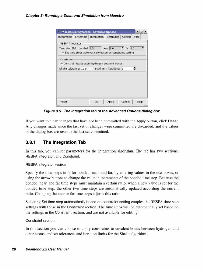
Figure 3.5. The Integration tab of the Advanced Options dialog box.
If you want to clear changes that have not been committed with the Apply button, click Reset.Any changes made since the last set of changes were committed are discarded, and the valuesin the dialog box are reset to the last set committed.
3.8.1 The Integration Tab
In this tab, you can set parameters for the integration algorithm. The tab has two sections,RESPA integrator, and Constraint.
RESPA integrator section
Specify the time steps in fs for bonded, near, and far, by entering values in the text boxes, orusing the arrow buttons to change the value in increments of the bonded time step. Because thebonded, near, and far time steps must maintain a certain ratio, when a new value is set for thebonded time step, the other two time steps are automatically updated according the currentratio. Changing the near or far time steps adjusts this ratio.
Selecting Set time step automatically based on constraint setting couples the RESPA time stepsettings with those in the Constraint section. The time steps will be automatically set based onthe settings in the Constraint section, and are not available for editing.
Constraint section
In this section you can choose to apply constraints to covalent bonds between hydrogen andother atoms, and set tolerances and iteration limits for the Shake algorithm.
Desmond 2.2 User Manual

Chapter 3: Running a Desmond Simulation from Maestro
Constrain heavy atom-hydrogen covalent bonds option
Select this option to constrain all bonds that are formed by a heavy atom and a hydrogen atomusing the Shake algorithm. Deselect this option to use bond potentials as defined in your modelsystem for these bonds.
Choice of this option affects the settings of the time steps when Set time steps automaticallybased on constraint setting is selected. With the constraint option selected, the bonded, near,and far time steps are set to 2 fs, 2 fs, and 6 fs, respectively; whereas with this option dese-lected, the time steps are set to 0.5 fs, 2 fs, and 6 fs, respectively. The larger time step permittedfor bonded interactions when constraints are used reduces the CPU time needed for a givenamount of simulation time.
Shake tolerance text box
Enter the tolerance used to check convergence of the relative bond length error for bondconstraints in the text box.
Maximum iterations text box
Enter the maximum number of iterations used in bond constraint calculations in this text box,or use the arrow buttons to change the value in increments of 1.
3.8.2 The Ensemble Tab
In this tab you can set the thermostat method and the barostat method and adjust the settingsfor these methods. The thermostat method and the barostat method are coupled: the choice youmake from the Thermostat method option menu changes the selection from the Barostatmethod option menu, and vice versa. The exception is that you can choose None for thebarostat method for any of the thermostat methods.
The Thermostat method option menu offers four choices: Nose-Hoover, Berendsen, Langevin,and None.
Although in most circumstances, only one thermostat group is needed, you can specifymultiple thermostat groups by entering the number of groups in the Number of groups text boxand supplying information on these groups in the Thermostat group settings table. Themaximum number of groups is 8. The selection of atoms that is in each group can be set up inthe Misc tab, by defining multiple groups named thermostat, with the group numbers corre-sponding to the entries in the Values column. Any atoms not explicitly added to a group areautomatically assigned to group 0, the default group. This means that you do not need to definea group if you only want to use one thermostat, and that you only need to define groups for theextra thermostats, starting from thermostat 1.
Desmond 2.2 User Manual 29

Chapter 3: Running a Desmond Simulation from Maestro
30
Figure 3.6. The Ensemble tab of the Advanced Options dialog box.
The Thermostat group settings table provides text boxes for making settings for each thermo-stat group. For the Nosé-Hoover method, you can also make barostat settings. The settings thatcan be made are:
• Reference temperature (K)• Relaxation time (ps) (not for Langevin)
Nosé-Hoover only:
• Chain length• Update frequency
The Barostat method option menu also offers four choices: Martyna-Tobias-Klein, Berendsen,Langevin, and None. For each of these methods you can set the relaxation time (ps) in theRelaxation time text box, choose a coupling style from the Coupling style option menu, and seta reference pressure in the Reference pressure text box. The coupling style choices areIsotropic, Semi-isotropic, and Anisotropic. For the Berendsen barostat, you can also enter thecompressibility in the Compressibility text box.
Desmond 2.2 User Manual

Chapter 3: Running a Desmond Simulation from Maestro
Figure 3.7. The Minimization tab of the Advanced Options dialog box.
3.8.3 The Minimization Tab
In this tab you can set parameters for the minimization, and also specify the output file. Mini-mization is performed with the LBFGS method, with an optional steepest descent initial phase.
The Minimizer section provides the following controls:
• LBFGS vectors—Specify the number of history vectors used by the LBFGS minimizerfor the update of the Hessian. The maximum is 6.
• Minimum SD steps—Specify the minimum number of steepest descent steps to be usedbefore switching to the LBFGS minimizer.
• Maximum step size—Specify the maximum step size in angstroms.
• Gradient threshold—Specify the gradient value in kcal mol–1 Å–1 at which the minimiza-tion method switches from steepest descent to LBFGS. The gradient is checked only afterthe minimum number of steps is performed.
In the Output section you can specify the name of the structure output file. You can use$JOBNAME as a variable representing the job name that you will set when you start the job orwrite out the input files. You can also select Monitor structural change in minimization if youwant results returned to the Workspace during the course of the minimization.
Desmond 2.2 User Manual 31

Chapter 3: Running a Desmond Simulation from Maestro
32
Figure 3.8. The Interaction tab of the Advanced Options dialog box.
3.8.4 The Interaction Tab
In this tab you can specify how the short-range and long-range Coulombic interactions arehandled.
To define the short-range region, choose a method from the Short range method option menu.The controls below this menu depend on the method chosen, which can be one of thefollowing:
• Cutoff—Enter a value in the Cutoff radius text box. The default is 9.0 Å.
• Force tapering or Potential tapering—Specify the range in angstroms over which theforce or the potential is tapered off in the two Tapering range text boxes.
There are two choices for handling the long-range Coulombic interactions:
• Smooth particle mesh Ewald—use the smooth particle mesh Ewald method. This methodrequires a tolerance to be set in the Ewald tolerance text box. This tolerance affects theaccuracy of the long-range Coulombic interactions. The smaller the tolerance is, the moreaccurate the computation of the long-range Coulombic interactions is, but the simulationwill be correspondingly slower.
• None—use the unmodified Coulomb interaction.
Desmond 2.2 User Manual

Chapter 3: Running a Desmond Simulation from Maestro
Figure 3.9. The Restraints tab of the Advanced Options dialog box.
3.8.5 The Restraints Tab
In this tab you can specify restraints on atom positions. A restraint is defined by a set of atomsand a force constant. The restraints are listed in the restraints table. The Atoms column is filledin automatically when you click Select and use the Atom Selection dialog box to specify theatoms. You must enter the force constant in the table manually, by editing the table cell.
To manage the restraints, you can use the buttons beside the table:
• Select—Opens the Atom Selection dialog box to specify the atoms for the selectedrestraint. Only available if a single row is selected in the table.
• Add—Adds a row to the restraints table so that a new restraint can be defined.
• Delete—Deletes the selected restraints.
• Reset—Resets the table to its default state.
3.8.6 The Output Tab
In this tab you can set names for various output files, and set the times for which recording inthese files begins, and the update frequency. For each file there is a starting time text box, inwhich you can enter the starting time for recording of information to this file or adjust thestarting time in increments of 50 times the far time step (except for the checkpoint file, wherethe increment is 5000 times the far time step). Some files also have an interval text box, inwhich you can enter or adjust the recording interval (in the same increments as the starting
Desmond 2.2 User Manual 33

Chapter 3: Running a Desmond Simulation from Maestro
34
time). The files are listed below, with any extra controls. The intervals for the energy sequencefile and for the trajectory can be set in the Desmond panel.
• Status message file—This file contains general information about the current status ofthe simulation.
• Energy sequence file—This file contains a sequence of various energies of the system.
• Trajectory directory—This directory is used by Desmond to periodically write out filesthat record coordinates and velocities (optional) of all particles in the system at a particu-lar point in the simulation. You can provide a title for the trajectory, and you can selectRecord velocities if you want the velocities to be recorded along with the coordinates.
To ensure that associated solutes appear together in the trajectory rather than on oppositesides of the simulation box, you can select Glue close solute molecules together. Thisoption only affects the way the trajectory is displayed.
• Checkpoint file—This file contains information that can be used to restart an interruptedsimulation. Checkpoint files permit bitwise continuation of simulations, so they can belarge, and should be saved infrequently if at all.
• Monitoring file—This file contains the coordinates of all particles in the system. This fileis in Maestro format and is used to monitor the progress of the simulation in Maestro.
Figure 3.10. The Output tab of the Advanced Options dialog box.
Desmond 2.2 User Manual

Chapter 3: Running a Desmond Simulation from Maestro
Figure 3.11. The Misc tab of the Advanced Options dialog box.
3.8.7 The Misc Tab
This tab provides access to various options that do not fit into the other categories. In this tabyou can initialize the velocities using a random number and a target temperature, and specifyatom groups for special treatment in the simulation.
Select Initialize velocities to initialize the velocities using the seed specified in the Randomnumber seed text box and the target temperature specified in the Target temperature text box,in kelvin.
In the Atom group section you can specify atom groups. Atom groups are used for variousspecial treatments of atoms in the simulation. For example, if you define the frozen atomgroup, the atoms in this group will be frozen in the simulation.
You can define multiple groups with the same name but a different index by setting the index inthe Value column. If you use multiple thermostats, for example, you can define the atoms ineach thermostat group by naming the group thermostat and setting the index to the thermo-stat group number in the Ensemble tab. Group 0 is the default group, to which all unassignedatoms automatically belong.
The atom groups are listed in the table. The Atoms column is filled in automatically when youclick Select and use the Atom Selection dialog box to specify the atoms. Otherwise you canedit this column to specify the ASL expression for the atoms in the group. The number ofatoms defined by the ASL expression is shown in the No. of Atoms column.
Desmond 2.2 User Manual 35
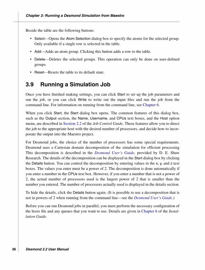
Chapter 3: Running a Desmond Simulation from Maestro
36
Beside the table are the following buttons:
• Select—Opens the Atom Selection dialog box to specify the atoms for the selected group.Only available if a single row is selected in the table.
• Add—Adds an atom group. Clicking this button adds a row to the table.
• Delete—Deletes the selected groups. This operation can only be done on user-definedgroups.
• Reset—Resets the table to its default state.
3.9 Running a Simulation Job
Once you have finished making settings, you can click Start to set up the job parameters andrun the job, or you can click Write to write out the input files and run the job from thecommand line. For information on running from the command line, see Chapter 6.
When you click Start, the Start dialog box opens. The common features of this dialog box,such as the Output section, the Name, Username, and CPUs text boxes, and the Host optionmenu, are described in Section 2.2 of the Job Control Guide. These features allow you to directthe job to the appropriate host with the desired number of processors, and decide how to incor-porate the output into the Maestro project.
For Desmond jobs, the choice of the number of processors has some special requirements.Desmond uses a Cartesian domain decomposition of the simulation for efficient processingThis decomposition is described in the Desmond User’s Guide, provided by D. E. ShawResearch. The details of the decomposition can be displayed in the Start dialog box by clickingthe Details button. You can control the decomposition by entering values in the x, y, and z textboxes. The values you enter must be a power of 2. The decomposition is done automatically ifyou enter a number in the CPUs text box. However, if you enter a number that is not a power of2, the actual number of processors used is the largest power of 2 that is smaller than thenumber you entered. The number of processors actually used is displayed in the details section.
To hide the details, click the Details button again. (It is possible to use a decomposition that isnot in powers of 2 when running from the command line—see the Desmond User’s Guide.)
Before you can run Desmond jobs in parallel, you must perform the necessary configuration ofthe hosts file and any queues that you want to use. Details are given in Chapter 6 of the Instal-lation Guide.
Desmond 2.2 User Manual
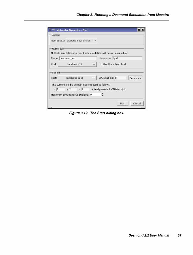
Chapter 3: Running a Desmond Simulation from Maestro
Figure 3.12. The Start dialog box.
Desmond 2.2 User Manual 37

38
Desmond 2.2 User Manual
Desmond User Manual
Chapter 4
Chapter 4: Running FEP Simulations
Maestro provides panels for quickly setting up FEP simulations for certain common scenarios:
• Mutation of ligand functional groups: a group attached to a ligand by a single bond ismutated to some other group.
• Aromatic ring atom substitution: an atom (with its attached hydrogens) is mutated intoanother atom, usually a heteroatom.
• Protein residue mutation: the side chain of a protein residue is mutated into that ofanother residue.
In these three scenarios, the binding free energy of the ligand can be calculated. For the firsttwo, the solvation free energy of the ligand relative to the original ligand can be calculated.
Total (absolute) solvation free energies can also be calculated for a ligand or a molecule, whichis done by annihilating the chosen molecule in the FEP simulation.
Free energy perturbation calculations are resource-intensive. While it is possible with the FEPpanels to set up multiple mutations in a single calculation, we recommend that only one muta-tion be performed per calculation due to the resource requirements.
4.1 FEP Panels
The FEP panels are designed to make setting up FEP jobs as easy as possible: most of thecomputational details, such as setting the force field parameters, solvation, relaxation of thesystem, and simulation time, are taken care of automatically. These predetermined parametersfor the FEP calculations should work for most systems, but you can also write out the inputfiles and then modify the simulation parameters in the FEP panel—see Section 4.8 on page 50.(Note that checkpoint files are not written out for the relaxation stages.)
The panels for these calculation types have a common design. Each panel has a Define Pertur-bation tab, in which you set up the systems to be simulated, and a Plan Calculation tab, inwhich you choose the environment (complex, pure solvent, vacuum) for the ligand and choosethe FEP protocol, which includes the ensemble. Information on setting up the system iscontained in the next few sections, followed by a section describing the Plan Calculation tab.
Desmond 2.2 User Manual 39

Chapter 4: Running FEP Simulations
40
The panels have action buttons at the bottom:
• Start—Opens the Start dialog box, in which you can set the job parameters such as jobname, host, number of CPUs, and so on, and then start the job. The general layout of thisdialog box is described in Section 2.2 of the Job Control Guide. The Desmond-specificfeatures of the Start dialog box and the issues in choosing the number of CPUs aredescribed in Section 3.9 on page 36.
• Write—Writes the input files for the job but does not start the job. Opens a dialog box inwhich you can specify a job name, which is used to name the files. This capability is use-ful if you want to change the FEP protocol.
• Reset—Resets the entire panel to its initial state. This includes clearing the Workspace. Ifyou want to use the same structures, you will have to redisplay them before proceeding.
4.2 Ligand Functional Group Mutation
In ligand mutation, a group on the ligand molecule, called the substitution group, is replacedwith selected fragments. These fragments are chosen from a list of small, predefined frag-ments. The fragments can be adjusted to reduce steric clashes, and can be modified by usingthe tools on the Build toolbar or in the Build panel.
The FEP calculations for ligand mutation are set up in the Ligand Functional Group Mutation byFEP panel, which you open by choosing Desmond from the Applications menu, then choosingLigand Functional Group Mutation by FEP.
To run a ligand mutation job:
1. Include in the Maestro Workspace the system that contains the ligand to be mutated, thereceptor protein (optional), and any other key molecules of the system.
This step can be performed prior to opening the panel.
2. Select Pick the attachment bond, then pick the attachment bond in the Workspace, at theend toward the substitution group.
This bond is the bond at which the substitution will take place. When the bond is picked,a green arrow is drawn over the bond, pointing to the substitution group, and the ligandcore is colored with green carbons. If you clicked on the wrong end of the bond, clickagain to correct the error. Once focus is returned to the panel, this option is deselected.
3. In the Fragment library table, select the fragments that you want to use to replace the orig-inal substitution group, by selecting their table rows.
Use shift-click and control-click to select multiple table rows. You can view the mutatedligand by clicking in the View column.
Desmond 2.2 User Manual

Chapter 4: Running FEP Simulations
Figure 4.1. The Ligand Functional Group Mutation by FEP panel, Define Perturbation tab.
Since each FEP mutation requires a large amount of CPU time and space, we recommendperforming only one mutation in a given calculation.
4. (Optional) Display the mutated ligand and make adjustments to the fragment.
The adjusted fragment is used as the starting point in the FEP simulations. It is possiblethat the fragment may have clashes with the protein in its default orientation or be in an inappropriate conformation. The barriers between local minima in the potential energy sur-face can be large, and thus take a long time to cross during a simulation. Adjusting theconformation can reduce clashes and help the simulation to sample the appropriateconformations.
Once the fragment is displayed, you can reorient the fragment with the adjustment tools,which are available from the Adjust toolbar button:
Desmond 2.2 User Manual 41

Chapter 4: Running FEP Simulations
42
or with the local transformation tools, which are available from the Local transformationtoolbar button:
For more information on these tools, see Section 4.8 and Section 7.2 of the Maestro UserManual.
You can also add to the fragment using the Build toolbar or the Build panel—for example,replacing a hydrogen with a methyl or a hydroxyl group. Since the quality of the resultsgoes down as you increase the size of the fragment, it is not advisable to add too much tothe fragment.
You can revert to the original fragment by clicking the button in the Reset column. Youshould not make modifications to the ligand core or other molecules in the system.
5. In the Plan Calculation tab, select the calculation types:
• For binding free energy calculations, select In complex and In pure solvent.• For solvation free energy calculations, select In pure solvent and In vacuum.
6. Choose the FEP protocol you want to use for each calculation type from the FEP protocoloption menu.
You should choose the same ensemble type for both the complex and pure solventcalculations.
7. Click Start, set the job parameters in the Start dialog box, and click Start in the dialogbox to run the job.
4.3 Ring Atom Mutation
Ring atom mutation changes a selected ring atom to a different atom type while preserving thehybridization of the atom.
To run a ring atom mutation job:
1. Include in the Maestro Workspace the system that contains the ligand to be mutated, thereceptor protein (optional), and any other key molecules of the system.
This step can be performed prior to opening the panel.
2. Select Pick the ring atom, then pick the ligand atom to be mutated in the Workspace.
Desmond 2.2 User Manual

Chapter 4: Running FEP Simulations
Figure 4.2. The Ring Atom Mutation by FEP panel, Define Perturbation tab.
When the atom is picked, it is rendered in ball-and-stick, and the ligand is colored withgreen carbons. The Mutation targets table is displayed. Once focus is returned to thepanel, this option is deselected.
3. In the Mutation targets table, select the targets that you want to use to replace the originalring atom by selecting their table rows.
Use shift-click and control-click to select multiple table rows. You can view the mutatedligand by clicking in the View column. If you want to add a functional group as well asmutate the ring atom, you can use the build tools to add to the mutated structure.
4. In the Plan Calculation tab, select the calculation types:
• For binding free energy calculations, select In complex and In pure solvent.• For solvation free energy calculations, select In pure solvent and In vacuum.
5. Choose the FEP protocol you want to use for each calculation type from the FEP protocoloption menu.
Desmond 2.2 User Manual 43
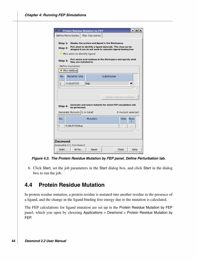
Chapter 4: Running FEP Simulations
44
Figure 4.3. The Protein Residue Mutation by FEP panel, Define Perturbation tab.
6. Click Start, set the job parameters in the Start dialog box, and click Start in the dialogbox to run the job.
4.4 Protein Residue Mutation
In protein residue mutation, a protein residue is mutated into another residue in the presence ofa ligand, and the change in the ligand binding free energy due to the mutation is calculated.
The FEP calculations for ligand mutation are set up in the Protein Residue Mutation by FEPpanel, which you open by choosing Applications > Desmond > Protein Residue Mutation byFEP.
Desmond 2.2 User Manual

Chapter 4: Running FEP Simulations
To run a protein residue mutation job:
1. Include in the Maestro Workspace the system that contains the ligand to be mutated, thereceptor protein, and any other key molecules of the system.
This step can be performed prior to opening the panel.
2. Select Pick atom to identify ligand, then pick a ligand atom in the Workspace.
3. In the Define Mutations section, select Pick residue.
4. Pick a protein residue in the Workspace.
The residue is added to the table as a mutation site.
5. In the Substitutes column, choose the residue from the list that you want to use to replacethe original.
To open the list, click the arrow button. The arrow changes direction and the list is dis-played. To close it click the arrow button again.
6. Repeat Step 4 and Step 5 for as many mutations as you want to perform.
You can pick the same residue multiple times to mutate it to different residues. If youpick different residues, each residue that you pick is mutated.
7. Click Generate Mutants.
8. The table is filled with the mutations that you have defined. For each of the original resi-dues that you picked, all possible combinations of mutations are added to the table. Forexample, if you picked two different residues, and for each you specified three substi-tutes, the table would list nine mutations, corresponding to each possible combination.
9. In the mutants table, select the mutations that you want to use, by selecting their tablerows.
Use shift-click and control-click to select multiple table rows. You can view the mutatedligand by clicking in the View column.
Once the residue is displayed, you can reorient the side chain with the adjustment tools,which are available from the Adjust toolbar button:
or with the local transformation tools, which are available from the Local transformationtoolbar button:
Desmond 2.2 User Manual 45

Chapter 4: Running FEP Simulations
46
For more information on these tools, see Section 4.8 and Section 7.2 of the Maestro UserManual.
You can also modify the residue using the Build toolbar or the Build panel—for exampleto replace sulfur with selenium, or to phosphorylate the residue. Since the quality of theresults goes down as you increase the size of the perturbation, it is not advisable to addtoo much to the residue.
You can revert to the original residue orientation and structure by clicking the button inthe Reset column. You should not make modifications to the ligand core or other mole-cules in the system.
10. In the Plan Calculation tab, choose the FEP protocol you want to use for each calculationtype from the FEP protocol option menu.
You should choose the same ensemble type for both the complex and pure solventcalculations.
11. Click Start, set the job parameters in the Start dialog box, and click Start in the dialogbox to run the job.
4.5 Total Solvation Free Energy Calculation
Calculating the absolute solvation free energy for a molecule involves running an “annihila-tion” FEP simulation, in which the selected molecule is removed from the system.
To run an annihilation job:
1. Include in the Maestro Workspace the system that contains the molecule to be annihi-lated.
This step can be performed prior to opening the panel.
2. Select Pick the molecule, then pick the molecule in the Workspace.
When the molecule is picked, it is colored with green carbons. Once focus is returned tothe panel, this option is deselected.
3. In the Plan Calculation tab, ensure that In pure solvent is selected.
4. Choose the FEP protocol you want to use for each calculation type from the FEP protocoloption menu and make any related settings.
The default simulation time is 2 ns, which is recommended for accurate results.
5. Click Start, set the job parameters in the Start dialog box, and click Start in the dialogbox to run the job.
Desmond 2.2 User Manual

Chapter 4: Running FEP Simulations
Figure 4.4. The Total Free Energy by FEP panel, Define Perturbation tab.
4.6 Selecting the Environment and FEP Protocol
The selection of the ligand environment and FEP protocol is made in the Plan Calculation tab.
The FEP simulations can be performed in three ligand environments: in the protein-ligandcomplex (with solvent), in pure solvent, and in vacuum. This permits the calculation of bindingfree energies, by selecting In complex and In pure solvent, and of solvation free energies, byselecting In pure solvent and In vacuum.
The FEP protocol defines in detail how system is solvated, relaxed, and simulated. Four mainprotocols are provided in the FEP protocol option menu for the complex and pure solvent: twoensembles, Desmond NPT and Desmond NVT, with two options for the relaxation part (stan-dard, or quick relaxation). The protocol for the simulation is the same for both ensembles (NVTand NPT). For calculations in vacuum, there is the choice of the standard or quick relaxation.
Desmond 2.2 User Manual 47

Chapter 4: Running FEP Simulations
48
Figure 4.5. The Plan Calculation tab.
In addition you can read in a protocol by choosing User defined from the FEP protocol optionmenu. A file name text box and Browse button is displayed. You can enter the name of theprotocol file (which has a .msj extension) in the text box, or navigate to it in the file selectorthat opens when you click Browse.
The default protocol is as follows. The original system is solvated by adding SPC water mole-cules with a buffer distance of 5 Å for complexes and 10 Å for pure solvent. The vacuum simu-lation uses a buffer distance of 100 Å. The system goes through a relaxation process thatincludes two minimizations followed by 4 short molecular dynamics simulations. The produc-tion simulation is run for 0.6 ns for each lambda window, and 14 windows are used for eachperturbation. You can change the buffer size and the production simulation time for each envi-ronment in the Buffer size and Production simulation time text boxes.
After the production simulations, the results are collected and analyzed using the Bennettmethod. The final result (free energy) for each perturbation is recorded as an entry-level prop-erty in the final Maestro output file.
Desmond 2.2 User Manual

Chapter 4: Running FEP Simulations
4.7 FEP Results
The results of FEP calculations usually need some further processing to produce the quantitiesof interest. The most common of these are discussed in the sections below.
4.7.1 Relative Free-Energy Differences
The estimated changes in free energy for FEP calculations are recorded as structure-level prop-erties in the mutated structures (rather than in the original structures) in the output structurefile. For ligand functional group mutation, protein residue mutation and ring atom mutation,these values are displayed in Maestro as dG jobname, and recorded in the file ass_des_dG_jobname, where jobname is the name for the multisim job and usually ends in_vacuum, _solvent or _complex for the corresponding environments (vacuum, puresolvent, and complex). These values are strings rather than real numbers because they includethe estimated uncertainty. To obtain a relative solvation free energy, subtract the vacuum resultfrom the solvent result. Similarly relative binding free energies are calculated by subtractingthe solvent result from the complex result.
You can use the script calculate_ddg.py to take the difference between the values in twodifferent environments to provide a ∆∆G value. To run this script, use the following command:
$SCHRODINGER/run -FROM desmond calculate_ddg.py jobname1-out.maejobname2-out.mae [output-file.mae]
where jobname1-out.mae and jobname2-out.mae are the Maestro output structure filesfrom the two FEP calculations. The output file output-file.mae is optional; the default name isddG.mae. This file is in Maestro format and contains the ∆G value from both input files. Thefinal ∆∆G value is recorded for each mutant as an entry property s_des_ddG_jobname1-jobname2, which is displayed in the Project Table as ddG jobname1-jobname2. The atom coor-dinates in the output file are copied from the first input structure file.
4.7.2 Total Solvation Free Energies
The total absolute free energies calculated by Desmond are recorded in the output structure fileas structure-level properties for the solute structures. The property names ares_des_dg_jobname_transfer and s_des_dg_jobname_solvation. The former, thetransfer free energy, uses the same concentration in both the vacuum and solution phases whilethe latter, the solvation free energy, uses standard state concentrations in the two phases (1 barin vacuum and 1 Molal or 1 mole of solute per kg of solvent in solution).
When charged molecules are deleted or created in absolute free energy calculations, finite sizeeffects can be significant, particularly for the pure solvent FEP calculations. A script,
Desmond 2.2 User Manual 49

Chapter 4: Running FEP Simulations
50
calculate_correction.py, has been provided to provide a correction to the free energyonce the FEP calculation is complete. To run this script, use the following command:
$SCHRODINGER/run -FROM desmond calculate_correction.py jobname [data-dir]
where jobname is the name of the λ=0 simulation job for the original FEP calculation (e.g.,myfepjob_complex_4_lambda0). This program assumes the input and output file names arederived from jobname. Specifically, this program looks for the following files and directories:jobname-in.cms, jobname-in.cfg, and jobname_trj. jobname-in.cms and jobname-in.cfg must be the input files of the simulation, and jobname_trj is the trajectory directoryproduced during the simulation. The optional argument data_dir can be used to designate thename for the directory in which to look for the for the data files. If this argument is missing, thedefault directory name is jobname.
This program reviews the trajectory and calculates the correction. The final correction isprinted to standard output. During the process, the program writes out several files:jobname_correct1.cfg, jobname_correct1.log, and jobname_correct1.dat.Depending on your system, it may also write out the analogous files:jobname_correct2.cfg, jobname_correct2.log, and jobname_correct2.dat. Youneed not be concerned with the content of these files.
4.8 Customizing and Restarting FEP Simulations
FEP jobs perform a series of MD simulations for the calculation of the free energy differencebetween two systems. These simulations are set up in the specialized FEP panels describedearlier in this chapter. The FEP panel allows you to adjust FEP protocols set up in these panels,and to rerun lambda windows for FEP jobs that failed. To open the FEP panel, choose Applica-tions > Desmond > FEP in the main window.
The settings for the simulation time, recording interval, ensemble class, temperature, pressure,and model system relaxation are the same as for a molecular dynamics simulation, and aredescribed in Section 3.4 on page 20.
There are two options for the type of FEP that can be performed, that correspond to the typesof FEP that are set up with the specialized FEP panels:
• Mutate—Mutate one set of atoms into another. The atom set may be a molecule or a frag-ment. Select this option for ligand functional group mutation or ring atom mutation.
• Annihilate—Annihilate a set of atoms. Select this option for total free energy simulations.
You can specify the parameter for the soft-core potential used to eliminate van der Waalssingularities in the Soft-core parameter text box. It is not normally necessary to change thisvalue.
Desmond 2.2 User Manual

Chapter 4: Running FEP Simulations
Figure 4.6. The FEP panel.
The number of lambda windows you want to use can be entered in the Number of windows textbox. Each window is listed in the table below, with values for each of the six lambda parame-ters, Van der Waals, Charge, Charge, and Bonding, for the two systems, labeled A and B.
You can set the lambda values automatically, which is the default, or you can deselect Setlambda values automatically and edit the values for each window and each type of lambda. Thelambda values must be within the range [0, 1]. The background color of the cell is changed topink if the value is out of range, to warn that it must be set within the range.
The windows can be selected or deselected for the simulation using the buttons in the Windowindex row. You can also use the Select All Windows and Deselect All Windows buttons to selectall windows or clear the selection. For a new FEP job, all windows should normally be selected
Desmond 2.2 User Manual 51

Chapter 4: Running FEP Simulations
52
for simulation. If a simulation for a particular lambda window needs to be re-run, select onlythat window.
Desmond 2.2 User Manual

Desmond User Manual
Chapter 5
Chapter 5: Analyzing Simulations
5.1 Viewing Trajectories
You can play through trajectories, examine individual frames, and export trajectory data in avariety of forms, in the Trajectory panel. To open the Trajectory panel, click the T button in theAux column of the Project Table for the entry whose trajectory you want to view.
The toolbar in the Trajectory panel contains a standard set of controls for playing through thetrajectory frames, which are listed below. The menu bar has one menu, Play, which containsitems that correspond to the toolbar buttons.
Go to startDisplay the first frame.
PreviousDisplay the previous frame.
Play backwardDisplay the frames in sequence, moving toward the first.
StopStop playing through the frames.
Play forwardDisplay the frames in sequence, moving toward the last.
NextDisplay the next frame.
Go to endDisplay the last frame.
LoopChoose an option for repeating the display of the frames. Single direction displays frames ina single direction, then repeats. Oscillate reverses direction each time the beginning or end ofthe frame set is reached.
Desmond 2.2 User Manual 53

Chapter 5: Analyzing Simulations
54
Figure 5.1. The Trajectory panel.
You can control the selection of frames and the speed of play in the Frame control section ofthe panel.
• The Start and End text boxes define the frames at which play starts and ends. Frames arenumbered from 0.
• The Frame slider and frame text box can be used to select the frame to view. The currentframe number is displayed in the text box below the slider. The total number of frames isalso displayed in a noneditable text box.
• The Step text box sets the number of frames to step when playing through frames. Thisvalue does not affect the Frame slider. The frames that are selected for play can beexported as a selection of frames, using the output buttons.
Desmond 2.2 User Manual
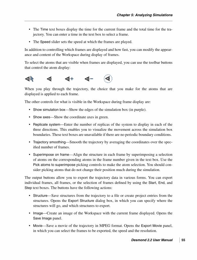
Chapter 5: Analyzing Simulations
• The Time text boxes display the time for the current frame and the total time for the tra-jectory. You can enter a time in the text box to select a frame.
• The Speed slider sets the speed at which the frames are played.
In addition to controlling which frames are displayed and how fast, you can modify the appear-ance and content of the Workspace during display of frames.
To select the atoms that are visible when frames are displayed, you can use the toolbar buttonsthat control the atom display:
When you play through the trajectory, the choice that you make for the atoms that aredisplayed is applied to each frame.
The other controls for what is visible in the Workspace during frame display are:
• Show simulation box—Show the edges of the simulation box (in purple).
• Show axes—Show the coordinate axes in green.
• Replicate system—Enter the number of replicas of the system to display in each of thethree directions. This enables you to visualize the movement across the simulation boxboundaries. These text boxes are unavailable if there are no periodic boundary conditions.
• Trajectory smoothing—Smooth the trajectory by averaging the coordinates over the spec-ified number of frames.
• Superimpose on frame—Align the structure in each frame by superimposing a selectionof atoms on the corresponding atoms in the frame number given in the text box. Use thePick atoms to superimpose picking controls to make the atom selection. You should con-sider picking atoms that do not change their position much during the simulation.
The output buttons allow you to export the trajectory data in various forms. You can exportindividual frames, all frames, or the selection of frames defined by using the Start, End, andStep text boxes. The buttons have the following actions:
• Structure—Save structures from the trajectory to a file or create project entries from thestructures. Opens the Export Structure dialog box, in which you can specify where thestructures will go, and which structures to export.
• Image—Create an image of the Workspace with the current frame displayed. Opens theSave Image panel.
• Movie—Save a movie of the trajectory in MPEG format. Opens the Export Movie panel,in which you can select the frames to be exported, the speed and the resolution.
Desmond 2.2 User Manual 55

Chapter 5: Analyzing Simulations
56
Figure 5.2. The Simulation Quality Analysis panel.
If you want to view a trajectory while a simulation is running, you can do so by importing thejobname-out.cms file for the simulation from the host on which the simulation is running.This file contains information on the location of the trajectory, and should be in the temporarydirectory for the job. There may also be a copy of the output CMS file in the working directoryon the local host, but the trajectory will not be present until the job finishes. Once you haveimported the file, click the T button for the imported entry. To update the trajectory later, youmust reimport the file.
5.2 Simulation Quality Analysis
The Simulation Quality Analysis panel displays a simulation summary and an analysis of thetotal energy, potential energy, temperature, pressure, and volume over the length of the simula-tion. The analysis includes the average value, the standard deviation, and the slope of a linearfit to the values of the property as a function of time. You can run the analysis on a completedsimulation or while the simulation is running.
To open the Simulation Quality Analysis panel, choose Applcations > Desmond > Simulation inthe main window.
To load the desired simulation, click Browse, and navigate to the desired Energy Sequence filefor the simulation, which has a .ene suffix. If you want to perform the analysis on a runningsimulation, you must use the file from the host on which the simulation is running.
Desmond 2.2 User Manual

Chapter 5: Analyzing Simulations
The analysis performs averaging of the results over short time periods (“blocks”) to reduce thenoise and eliminate correlation between consecutive reports. To change the size of the box,enter a value in the Box length for averaging text box.
When you have the desired box length, click Analyze to perform the analysis. The analysis cantake a few minutes. When it finishes, the Simulation summary and Properties sections are filledin with the results of the analysis. If you want to view a plot of the thermodynamic propertiesas a function of simulation time, click Plot. A panel is displayed with the results plotted.
You can also use the Simulation Event Analysis panel, which is not provided with the softwaredistribution, but is available from the Script Center. This panel can be used to investigate whathappened during a simulation.
Desmond 2.2 User Manual 57

58
Desmond 2.2 User Manual
Desmond User Manual
Chapter 6
Chapter 6: Running Desmond Simulations fromthe Command Line
Desmond jobs may be started from Maestro or from the command-line. The mechanisms forrunning jobs from the command line are described in this chapter. You might wish to runDesmond from the command line for any of the following reasons:
• To exercise greater control over Desmond behavior• To debug an aberrant run• For convenience• To transfer the job to a remote location
The Desmond panels can be used to write out (using the Write button) .cfg files for a simula-tion. Those .cfg files can then be run elsewhere, routinely from a batch script or customizedprior to use. More information on the contents of .cfg files is available in Appendix C.
Desmond jobs run under Schrödinger’s Job Control facility. This facility manages the execu-tion and monitoring of jobs, and handles the input and output files and the incorporation ofresults into a Maestro project. The Job Control Guide describes how to set up the informationneeded for Job Control to run on the computers to which you have access. It includes informa-tion on remote hosts, clusters, and batch queues.
As is the case for all Schrödinger software, the environment variable SCHRODINGER must beset to the directory where the Schrödinger software, including Desmond, was installed. Inaddition, there are other environment variables that can be set to override default resourcevalues. See Appendix B of the Job Control Guide for more information.
By default, the Schrödinger job control facility uses ssh to communicate between remotenodes. For more information, see Section 6.2 of the Installation Guide.
This chapter describes the command syntax for running single-stage and multistage Desmondjobs, and for building the input composite model system. For details of the file formats andtechnical background, see the Desmond User’s Guide, from D. E. Shaw Research.
6.1 The desmond Command
Desmond is run from the command-line by executing the shell script desmond, which islocated in the $SCHRODINGER directory. The desmond script determines the proper executa-bles to run for the host being used. Additional utility programs are provided in the$SCHRODINGER/utilities directory.
Desmond 2.2 User Manual 59

Chapter 6: Running Desmond Simulations from the Command Line
60
The syntax for the desmond command is as follows:
$SCHRODINGER/desmond [options] -in cms-file -c config-file$SCHRODINGER/desmond [options] -restore checkpoint-file
Use the -in option for a new job, and the -restore option for restarting a job. The input filefor a new job must be a CMS file, with extension .cms, and a configuration file (.cfg) mustalso be specified. For restarting a job, a checkpoint file, with extension .cpt, must beprovided.
The options for the desmond command are listed in Table 6.1. The standard Job Controloptions are also supported—see Section 2.3 of the Job Control Guide. Additional diagnosticoptions, which do not run the job but provide information, are also given in the sectionmentioned. In particular, you should note the syntax of the -HOST option, which is used tospecify the list of hosts used for the job.
For information on storage of temporary files, interacting with running Desmond jobs, and soon, see the Job Control Guide.
Table 6.1. Options for the desmond command.
Option Description
Job Options
-DEBUG Print diagnostic output.
-LOGINTERVAL Interval for copying the log file back to the submission host. Default: 5s.
-INTERVAL Interval for copying monitor files back to the submission host. Default:5s.
-p|-P|-PROCS|-NPROC Number of processors to use. Default: 1.
-JOBNAME name Specify the name for the job. The default is the input .cfg or .cpt filename, minus the extension.
-jin filename Files to be transferred to the execution host by Job Control.
-jout filename Files to be copied back to the submission host by Job Control.
-h[elp]|-HELP Print usage information
-v print version information and exit
Desmond 2.2 User Manual

Chapter 6: Running Desmond Simulations from the Command Line
Some examples of running desmond from command line are shown below:
1. Running a 4-processor job on a queuing system or a particular machine (myhost):
$SCHRODINGER/desmond -HOST myhost -P 4 -c x.cfg -in x.cms
2. Running a 4-processor job on two different machines (host1 and host2):
$SCHRODINGER/desmond -HOST host1:2 host2:2 -P 4 -c x.cfg -in x.cms
3. Continuing a 4-processor simulation from a checkpoint file (x.cpt):
$SCHRODINGER/desmond -HOST myhost -P 4 -restore x.cpt
4. Running a minimization job on a queuing system or a particular machine (ahost):
$SCHRODINGER/desmond -HOST ahost -c x.cfg -in x.cms -exec minimize
5. Running an energy calculation with an existing trajectory on a queuing system or a par-ticular machine (myhost):
$SCHRODINGER/desmond -HOST myhost -c x.cfg -in x.cms -exec vrun
6. Running a replica exchange simulation, in which each replica uses 2 processors with thesame input cms file:
Program Options
-exec program Run the specified Desmond program. Available programs are:mdsim—Run a molecular dynamics simulation (the default)minimize—Run a minimizationremd—Run a replica exchange molecular dynamics simulationvrun—Analyze a trajectory
-c config-file Parameter file for simulation. Required with -in for a new simulation.
-cfg key=val Specify extra simulation parameters. Multiple instances of this optioncan be supplied to specify multiple extra parameters.
-comm plugin Use the specified communication plugin. Available plugins are serialand mpi. Default: serial.
-dp Run double-precision version. Default: run single-precision version.
-noopt Do not optimize parameters automatically.
-t temperature Specify temperature in a replica exchange MD simulation. Include aninstance of this option for each temperature in the exchange.
-tpp n Specify the number of threads per processor.
Table 6.1. Options for the desmond command. (Continued)
Option Description
Desmond 2.2 User Manual 61

Chapter 6: Running Desmond Simulations from the Command Line
62
desmond -P 4 -c x.cfg -t 300 -t 310 -in x.cms -exec remd
7. Running a replica exchange simulation, in which each replica uses 2 processors with dif-ferent input cms files:
desmond -P 4 -c x.cfg -t 300 -in x300.cms -t 310 -in x310.cms \-exec remd
8. Restarting a replica exchange simulation from a checkpoint file (x.cpt):
desmond -P 4 -restore x.cpt -exec remd
6.2 Running Multiple Simulations
Molecular dynamics studies usually involve performing a series of calculations. For example, asequence of minimization, thermalization, and relaxation calculations followed by the produc-tion simulation itself is usually undertaken for molecular dynamics study. The MultiSim utility(multisim) facilitates the task of running multiple Desmond-related or MCPRO+-relatedcalculations in a sequential manner. The Desmond general and FEP panels can be used to writeout .msj files for those tasks. These .msj files can then be run elsewhere, for example from abatch script, or customized prior to use. More information on the contents of .msj files isavailable in the Maestro online help—see the list of Desmond topics.
The syntax for the multisim utility is as follows:
$SCHRODINGER/utilities/multisim [options] -i structure-file -m msj-file$SCHRODINGER/utilities/multisim [options] -r checkpoint-file
The first syntax should be used for new jobs, and the second for restarting jobs. The structurefile can be either a Maestro (.mae) file or a CMS (.cms) file. The options are described inTable 6.2, including job options. The standard Job Control options are also supported, as arethe options -LOCAL, -WAIT, and -NOJOBID—see Section 2.3 of the Job Control Guide.
Desmond 2.2 User Manual

Chapter 6: Running Desmond Simulations from the Command Line
Table 6.2. Options for the multisim utility.
Option Description
-ADD_FILE filename Additional input file to copy to the working directory of themultisim job. By default, multisim identifies and copies most filesneeded for the run.
-cfg cfg-file File that contains the default Desmond config parameters. This optionis only useful for Desmond subjobs.
-cpu num-cpus Number of CPUs for each Desmond subjob. This can be a string indi-cating the CPU topology e.g., '2 2 2'. If this option is not provided,a default value set by either the backend or the protocol will be used.All CPU counts must be a power of 2.
-d stage-file File containing information on the stages from the previous job, whenrestarting a simulation. Use one instance for each file.
-debug Turn on multisim debug mode.
-DEBUG Turn on both multisim and Job Control debug modes.
-description string Job description to print to the log file.
-h[elp], -HELP Print usage message and exit.
-host compute-host Host on which to run the subjobs.
-HOST multisim-host Host to run the multisim master job.
-JOBNAME jobname Job name of this multisim job
-max_retries maxretries Maximum number of times to restart failed subjobs
-maxjob maxjob Maximum number of simultaneous subjobs
-mode mode Run in non-default job management mode. The only allowed value isumbrella, for which subjobs run on the same node as the master job,-host is ignored and -maxjob is set to 1.
-o output-file Output .cms or .mae file. This file can be incorporated into Maestro.
-probe Probe a checkpoint file and quit.
-quiet Light log information (default).
-set string Specify parameters that take precedence over those in the .msj file.
-v[ersion] Print the multisim version and exit.
-verbose Heavy log information
Desmond 2.2 User Manual 63

Chapter 6: Running Desmond Simulations from the Command Line
64
6.2.1 Examples of Running MultiSim
A simple multisim command can take the form:
$SCHRODINGER/utilities/multisim -i input.cms -m input.msj-host mycluster -JOBNAME multistage
which runs the multisim utility with the starting structure from input.cms. The instruc-tions for different stages of multisim are provided in input.msj. The job is run on the hostlabeled mycluster in the schrodinger.hosts file. The job name is multistage.
The following command uses a different host for the master job and the subjobs:
$SCHRODINGER/utilities/multisim -i input.mae -m input_fep.msj-HOST localhost -host kyla_para -JOBNAME example_fep_job-maxjob 6 -cpu “2 2 2”
The -HOST option specifies the host of the master job, whereas -host specifies the computehost for the subjobs. The keyword -maxjob 6 means that at most 6 subjobs are simulta-neously in the queue of the compute host. When one of the subjobs finishes the next subjob islaunched on the compute host. At any time, the number of the subjobs launched from themaster job does not exceed 6 on the compute host.
6.2.2 Sample MultiSim Job (.msj) File
An example .msj file is given below. The file syntax is described in full in Appendix B. Thefile is modular, consisting of a series of stages, each of which contains a list of keywords andvalue settings enclosed within braces. Lines beginning with # are comments and hence areignored.
# Desmond standard NPT relaxation protocol# All times are in the unit of ps.# Energy is in the unit of kcal/mol.task { task = "desmond:auto"}
minimize { max_steps = 2000 steepest_descent_steps = 10 convergence = 50.0 cfg_overwrite = { minimize.maeff_snapshot.interval = inf } restrain = { atom = solute force_constant = 50.0 }}
Desmond 2.2 User Manual

Chapter 6: Running Desmond Simulations from the Command Line
minimize { max_steps = 2000 steepest_descent_steps = 10 convergence = 5.0 cfg_overwrite = { minimize.maeff_snapshot.interval = inf }}
simulate { time = 12 timestep = "0.001 0.001 0.003"
ensemble = NVT_Ber # NPT | NPT_Ber | NVT | NVT_Ber | NVE temperature = 10.0 thermostat_relaxation = 0.1 resampling_period = 1.0
cfg_overwrite = { integrator.remove_com_motion = true mdsim.maeff_snapshot.interval = inf mdsim.checkpt.first = inf mdsim.eneseq.interval = 0.3 }
restrain = { atom = solute_heavy_atom force_constant = 50.0 }}
simulate { time = 12
ensemble = NPT_Ber # NPT | NPT_Ber | NVT | NVT_Ber | NVE temperature = 10.0 thermostat_relaxation = 0.1 barostat_relaxation = 50.0 resampling_period = 1.0
cfg_overwrite = { integrator.remove_com_motion = true mdsim.maeff_snapshot.interval = inf mdsim.checkpt.first = inf mdsim.eneseq.interval = 0.3 }
restrain = retain}
simulate { time = 24
Desmond 2.2 User Manual 65

66
ensemble = NPT_Ber # NPT | NPT_Ber | NVT | NVT_Ber | NVE thermostat_relaxation = 0.1 barostat_relaxation = 50.0 resampling_period = 1.0
cfg_overwrite = { integrator.remove_com_motion = true mdsim.maeff_snapshot.interval = inf mdsim.checkpt.first = inf mdsim.eneseq.interval = 0.3 }
restrain = retain}
simulate { time = 24
ensemble = NPT_Ber # NPT | NPT_Ber | NVT | NVT_Ber | NVE thermostat_relaxation = 0.1 barostat_relaxation = 2.0
cfg_overwrite = { integrator.remove_com_motion = true mdsim.maeff_snapshot.interval = inf mdsim.checkpt.first = inf mdsim.eneseq.interval = 0.3 }}simulate { cfg_file = "example.cfg" jobname = "$JOBNAME" dir = "." compress = ""}# Job launching command:# $SCHRODINGER/utilities/multisim -JOBNAME example -HOST master_job_host -hostsubjob_host -maxjob 0 -cpu "2 2 2" -i example.cms -m example.msj -cfg example.cfg -o example-out.cms
In the above example, the first stage, task, specifies the type of job that is run so that appro-priate defaults can be set. In this case desmond:auto indicates that it is a Desmond job andthat the type of job should be detected automatically.
The second stage is a minimization of the system over a maximum of 2000 steps. Of the 2000steps, the first 10 steps are be steepest descent. The convergence criterion is set rather looselyto 50.0 kcal mol-1Å-1. The solute is restrained with a force constant of 50.0 kcal mol-1Å-1. Themonitor file is not updated. The third stage is similar except that nothing is restrained.
Desmond 2.2 User Manual

Chapter 6: Running Desmond Simulations from the Command Line
The fourth stage sets up a 12 ps Berendsen NVT simulation. For this simulation, the tempera-ture is set to 10.0 K, and the thermostat relaxation is set to 0.1 ps. Resampling is done every1 ps. The solute atoms are restrained. Checkpointing and structure monitoring are turned off.Center-of-mass motion is removed and the .ene file is updated more frequently, at intervals of0.3 ps. Subsequent simulation stages follow with progressively more freedom until the secondlast stage when conditions resemble the production run.
The last stage is the production dynamics simulation. The simulation parameters could havebeen explicitly listed here as in the preceding stages. In this example, this stage simply refers toa Desmond .cfg file. The last line gives an example of how this .msj file could be run. Youwould need to change the options for the job.
More examples can be found in the $SCHRODINGER/mmshare-vversion/data/desmonddirectory. Detailed information on the syntax of .msj files is available in [Appendix].
6.2.3 Treatment of Intermediate Files
In general, the files from each stage are copied back to the launch directory as a gzipped tararchive with the name jobname_stage-number.tgz. The production simulation stage is treateddifferently and the files are directly copied back without being archived. This treatment wouldbe similar to a simple molecular dynamics simulation (i.e. not a multisim job). This allowsthe final output CMS file to be incorporated and the trajectory to be played as a normal job.
6.3 Building a Model System
To prepare a model system from the command line, you can use the system builder utility,system_builder,. You can choose to add solvent, ions, and insert the solute into amembrane. The system_builder utility takes a composite system builder (CSB) file asinput. This file contains all the required information to convert a solute file into a solvatedsystem.
The syntax of the system_builder command is as follows:
$SCHRODINGER/utilities/system_builder input.csb
The standard Job Control options, described in Table 2.1 of the Job Control Guide, areaccepted, as are the options -WAIT, -LOCAL, and -NOJOBID, described in Table 2.2 of the JobControl Guide.
The possible steps involved in the conversion are:
• Reading the solute from a file• Reading the water model
Desmond 2.2 User Manual 67

Chapter 6: Running Desmond Simulations from the Command Line
68
• Reading the positive ion data• Reading the negative ion data• Adding a membrane• Solvating• Neutralizing• Writing out a composite molecular system (CMS) file.
The order of the keywords in a CSB file matters. Lines beginning with # are considered to becomments and are ignored. An example CSB file is shown below:
{ read_solute_structure mysolute_setup-in.mae # solute file name solvent_desmond_oplsaa_typer { input_file_name spc.box.mae run } positive_ion_desmond_oplsaa_typer { input_file_name Na.mae run } negative_ion_desmond_oplsaa_typer { input_file_name Cl.mae run } membranize POPE.mae.gz 10.000000 10.000000 create_boundary_conditions orthorhombic 0.000000 0.000000 10.000000 exclude_ion_from { 1 2 } 10.0 solvate neutralize write_maeff_file chorus_setup-out.cms}
The various sections of the file are described in the following subsections.
6.3.1 Reading the Structures
The first five sections read in all the structural information for the solute, solvent, and ions. Tolocate the files that contain this information, the current directory is searched first, then thedirectory $SCHRODINGER/mmshare-vversion/data/system_builder.
The first section reads the solute and solvent structure.
read_solute_structure mysolute_setup-in.mae # solute file name solvent_desmond_oplsaa_typer { input_file_name spc.box.mae
Desmond 2.2 User Manual

Chapter 6: Running Desmond Simulations from the Command Line
run }
The keyword read_solute_structure reads the solute structure from the specified file. Ifthe file is given as a relative path, it is copied to the temporary directory for the job. If it isgiven as an absolute path, the file must exist at that location on the execution host. The struc-tures can be a solute structure, structures for different stages of FEP simulations, or acompletely solvated system. The force-field information is obtained by either reading from anexisting ffio_ff block in the input file or running the force field server.
The solvent_desmond_oplsaa_typer section describes the solvent system that is used tosolvate the structure. The keyword input_file_name specifies the file to be used to read thesolvent model.
The next two sections determine the data to be used for counter ions to neutralize (or in somecases charge) the system.
positive_ion_desmond_oplsaa_typer { input_file_name Na.mae run
}negative_ion_desmond_oplsaa_typer {
input_file_name Cl.mae run
}
These two sections describe the ion systems to neutralize or to add ions to the current struc-tures. In each section one input_file_name keyword is provided to determine the file to beused.
The next two sections (not used in the example file above) similarly determine the ion systemsto add salts to the system.
salt_positive_ion_desmond_oplsaa_typer { input_file_name Na.mae run}salt_negative_ion_desmond_oplsaa_typer { input_file_name Cl.mae run}
The syntax for this section is same as for the positive and negative ion sections.
Desmond 2.2 User Manual 69
Chapter 6: Running Desmond Simulations from the Command Line
70
6.3.2 Adding a Membrane
The keyword membranize instructs the system builder to create a membrane patch around thecurrent solute structure.
membranize filename x-buf y-buf
The first input parameter is the name of the file that includes the membrane template and itsequilibrating solvent. The other two parameters x-buf and y-buf specify the minimum distancebetween the solute and the box boundary in the plane of the membrane.
6.3.3 Setting the Box Shape and Dimensions
The box shape and dimensions can be specified either in terms of an absolute size or in termsof a buffer distance.
The keyword boundary_conditions is used to define a box with specified absolute dimen-sions. The command using this keyword can be one of the following:
boundary_conditions cubic aboundary_conditions orthorhombic a b cboundary_conditions triclinic a b c alpha beta gamma
The box shape is the first parameter, and can be cubic, orthorhombic, or triclinic. It isfollowed by the absolute size of the box defined by a or by a, b, and c. For a triclinic box shape,the angles alpha, beta, and gamma must also be given.
Alternatively, the keyword create_boundary_conditions can be used to specify a box interms of the distance between solute atoms and box edges. he command using this keywordcan be one of the following:
create_boundary_conditions cubic acreate_boundary_conditions orthorhombic a b ccreate_boundary_conditions triclinic a b c alpha beta gamma
The parameters are similar to those for the absolute box size, but the distances are theminimum distance any solute atom and the box boundary in the given direction. The distancebetween two images of the solute structures is therefore twice the specified values. If amembrane is used, the box shape must be orthorhombic and the a and b values must be set tozero so that solvent molecules are not placed within the membrane layers.
Desmond 2.2 User Manual

Chapter 6: Running Desmond Simulations from the Command Line
6.3.4 Setting Force Field Information
The command set_oplsaa_version can be used to specify OPLSAA version. Currentlyonly OPLS_2005 (value: 2005) is supported.
set_oplsaa_version 2005
6.3.5 Setting the Number and Location of Ions
The addition of ions to the system is governed by several keywords: add_ion,ion_location, exclude_ion_from, add_salt, and neutralize.
Two commands using the keyword add_ion can be used to add specific numbers of positiveand negative ions.
add_ion positive 5add_ion negative 5
The keyword add_ion adds positive or negative ions to the system. The number of ions to beadded is specified as the second argument of this keyword.
The ion_location keyword can be used to specify the proximity of ions with reference tocertain atoms.
ion_location { { atom1 } { atom2 } }
The keyword ion_location is followed by the list of solute atom indexes. Ions are placednear the listed atoms. For each ion, the atom index is given inside braces. Extra atom indexspecifications are ignored. If there are fewer atom index specifications than there are ions, theremaining ion locations are determined randomly.
In order to exclude ions near certain atoms, the exclude_ion_from keyword can be used:
exclude_ion_from { atom-list } distance
The keyword exclude_ion_from has two arguments. The first argument is a list of atomindices of solute atoms, in braces. The second argument is the distance value. No ion, whethera single ion or from a salt, is placed within the given distance in angstroms from the listedatoms.
The salt concentration is determined using the add_salt keyword.
add_salt conc
The keyword add_salt adds the positive and negative salt ions to the system defined above.The argument specifies the salt concentration for the molecular system. Based on the volume
Desmond 2.2 User Manual 71

Chapter 6: Running Desmond Simulations from the Command Line
72
of the solvent and the concentration, the number of salt ions is calculated and rounded to aninteger value. The coordinates of salt ions are determined randomly.
The following command can be used to neutralize the system.
neutralize
The net charge of the current solute structures is calculated and the number of counter ionsnecessary to neutralize the system is added.
6.3.6 Solvating the System
This command is used to initiate the solvation of the current solute structure, which includesthe ions and the membrane.
solvate
The keyword solvate is used to solvate the current solute structures using the solvent systemdefined in the solvent_desmond_oplsaa_typer section. The solvent system is extended tobe consistent with the boundary condition defined by the boundary_conditions orcreate_boundary_conditions section. Any solvent molecules that overlap the solutestructures are removed.
6.3.7 Writing the Output File
This command is used to write the output to a “maeff” (Maestro + force-field) file, otherwiseknown as a composite model system (CMS) file, which has the extension .cms.
write_maeff_file filename
The keyword write_maeff_file writes the current composite structures and their force fieldparameters into a file in CMS format. The first structure contains all of the molecules in thesystem and is usually referred to as the “full system CT”. The following structures containdifferent components of the system. For instance there usually is a solute structure, a solventstructure (containing all of the solvent molecules) and structures for different types of ions.The force field parameters are inserted as ffio_ff blocks within each CT block (“structure”)except the first.
Desmond 2.2 User Manual

Desmond User Manual
Chapter 7
Chapter 7: Using VMD for Desmond Trajectories
VMD [7] is a powerful program for visualizing molecular dynamics simulations that is avail-able from the Theoretical and Computational Biophysics Group at the University of Illinois atUrbana-Champaign. A plugin for VMD is provided as part of Desmond that makes it possiblefor VMD to read and write Maestro files and read Desmond trajectories. The output Maestrofiles are suitable for use in building model systems that can then be used to run Desmond.
This chapter contains information on installing VMD and the Desmond plugin, reading a CMSfile and a Desmond trajectory into VMD, and writing a Maestro file from VMD.
7.1 Installing VMD and the Desmond Plugin
The plugin currently only works with alpha versions of VMD, in particular version 1.8.7a19 ornewer; referred to as 1.8.7axx. The Desmond plugin is part of VMD from version 1.8.7a48 on,and does not need to be added to the VMD installation. You can download VMD using abrowser by following these steps:
1. Go to http://www.ks.uiuc.edu/Research/vmd/alpha/1
2. Log in to BioCoRE on this page.
If you do not already have an account you can request one from this page and then log in.
3. Download vmd-1.8.7axx.bin.LINUX.opengl.tar.gz
To install and configure VMD:
1. Extract the tar file:
tar -zxvf /zone1/lin/tmp/vmd-1.8.7axx.tgz
2. Change to the VMD directory:
cd vmd-1.8.7axx
3. Edit the configure file and set the values of install_bin_dir andinstall_library_dir to the locations where you wish to install the VMD binary andits supporting libraries.
1. Please see the notice regarding third party programs and third party Web sites on the copyright page at the frontof this manual.
Desmond 2.2 User Manual 73

Chapter 7: Using VMD for Desmond Trajectories
74
4. Run the configuration:
./configure
5. Install VMD:
cd srcmake install
6. Make sure that the directory containing the vmd executable (the one that you listed forinstall_bin_dir inside the configure file above) is in the path for your shell.
For instance, if that directory was /usr/local/bin/vmd-1.8.7 and you are using thebash shell you could use the following command:
PATH=$PATH:/usr/local/bin/vmd-1.8.7
7. If you are installing a version of VMD earlier than 1.8.7a48, copy the two plugin filesinto the VMD library directory:
cp $SCHRODINGER/desmond-vversion/lib/arch/vmd_plugins/*install-library-dir/vmd/plugins/LINUX/molfile
where arch is Linux-x86 for 32-bit platforms and Linux-x86_64 for 64-bit platforms.
8. On 64-bit platforms, add $SCHRODINGER/desmond-vversion/lib/Linux-x86_64 toyour LD_LIBRARY_PATH environment variable.
You should now be able to run VMD and use the VMD plugin. You can start VMD by typingthe command:
vmd
Two windows are opened, VMD main and VMD version OpenGL Display. The former can beused to control VMD while the latter can be used to display the molecular systems and to viewtrajectories. VMD has extensive documentation which is available from the Help menu in theVMD main window.
Desmond 2.2 User Manual

Chapter 7: Using VMD for Desmond Trajectories
7.2 Reading a CMS File and a Desmond Trajectory
This section describes how to read a Maestro CMS file and a Desmond trajectory into VMD.To view a Desmond trajectory in VMD, you must first read in the output structure CMS filefrom a Desmond simulation. This file is usually named jobname-out.cms. Viewing trajecto-ries from Desmond FEP simulations is not currently supported.
To read in a CMS file:
1. Choose New Molecule from the File menu of the VMD Main window.
The Molecule File Browser panel opens.
2. Click Browse.
A file selector opens.
3. Navigate to and select the output .cms file from a Desmond simulation, and click OK.
The file selector closes.
4. In the Molecule File Browser panel, set the file type to Maestro File (no timesteps).
5. Click Load.
You have just created a Molecule listing in VMD which should appear as a new a line in theVMD Main window corresponding to the CMS file that you just read in.
To read in a trajectory for this system:
1. Ensure that the line for the CMS file that you just read in is the only one that is high-lighted.
2. Choose Load Data into Molecule from the File menu in the VMD Main window.
The Molecule File Browser panel opens.
3. Click Browse.
A file selector opens.
4. Navigate into the trajectory directory from a Desmond simulation.
5. Select the file clickme.dtr and click OK.
The file selector closes. In the Molecule File Browser the file type should now be listed asDesmond trajectory.
6. Click Load.
The trajectory should load into VMD and automatically start playing.
Desmond 2.2 User Manual 75

Chapter 7: Using VMD for Desmond Trajectories
76
7.3 Writing a Maestro File
You can export individual configurations into a Maestro file from within VMD. This can be auseful way to convert configurations produced by various programs into a format that willfunction with Maestro.
To export a Maestro file from VMD:
1. Select the molecule that you want to export in the VMD main window.
2. Choose Save Coordinates from the File menu.
The Save Trajectory panel opens.
3. Set the File type to mae0.
4. Click Save.
5. In the Filename text box, edit the directory, and append the name for the new file to thedirectory.
This is a plain Maestro file, whose extension should be .mae.
6. Click OK.
Desmond 2.2 User Manual

Desmond User Manual
Chapter 8
Chapter 8: Using Alternate Force Field Parametersand Constraints
The Desmond installation includes two utilities, viparr and build_constraints that canbe used to add or adjust the force field parameters and the accompanying constraints for chem-ical systems prior to simulating them with Desmond. Both programs read and write Maestrostructure files.
Viparr is a template-based force field assignment utility that comes with a number of built-inforce fields including some developed for Amber and CHARMM (see below for more informa-tion). User-defined force fields are also supported by viparr, if they are provided in viparr’s fileformat. Viparr can be used to specify different force fields for various components of thesystem, provided that the force fields are compatible. This flexibility makes it possible to dosome things that may be useful in force-field development including:
• Using one force field for one part of the chemical system and another force field foranother part (this allows you, for example, to easily switch between water models)
• Using one or more components from one force field (e.g., the dihedral parameters) andthe remaining components from another force field
• Overriding some of the parameters (e.g., some but not all of the angle parameters) withthose from another force field
Some classes of constraints are often used with, and in some cases required by, various forcefield representations of molecules. The utility build_constraints may be used to add theconstraints to a structure file.
8.1 The viparr Utility
To run viparr, use the following command:
$SCHRODINGER/run -FROM desmond -viparr.py [options] input-file output-file
where input-file and output-file are the input and output structure (CMS) files, respectively.This utility does not run under Job Control. It does not take much time, so it can be run locally.
The basic options are given in Table 8.1. The force field data files are located in the directory$SCHRODINGER/desmond-vversion/data/viparr.
Desmond 2.2 User Manual 77

Chapter 8: Using Alternate Force Field Parameters and Constraints
78
The available force fields are listed in Table 8.2, with references.
Table 8.1. Options for the viparr utility.
Option Description
-h Print usage message, including the names of the built-in force fields
-n name Specify force field name or other annotation to put into the output file. If not spec-ified, a default name is used.
-f ffname Specify a built-in force field. The available force fields are listed in Table 8.2. Youcan repeat this option to specify multiple force fields, one per instance of theoption. Parameters of force fields listed earlier override parameters of force fieldslisted later. When multiple force fields are specified, the order is important if someparameters are intended to override others.
-c ctnum Specify the index of a single structure (“CT block”) in the input file for processingby viparr. Structures are numbered starting at 1. Only a single -c option isallowed on the command line: you cannot specify more than one structure to pro-cess. The default is to process all structures.
-d ffdir Specify a user-defined force-field directory. You can repeat this option to specifymultiple directories. As for -f, the order is important.
-m mergedir Path to user-defined force field directory that is to be merged with previously spec-ified force field. Multiple directories can be specified with multiple instances ofthis option.
-p pdir Specify the plugin directory. The default is to use the directory defined by theenvironment variable VIPARR_PDIR, which contains the standard plugins. Allnecessary plugins, including those for the built-in force fields, must be in thedirectory specified by -p.
Table 8.2. Force fields available with viparr.
Force Field Ref. Force Field Ref.
Amber Water models
amber94 [8] spc [24]
amber96 [9] spce [25]
amber99 [10] tip3p [26]
amber99SB [10,11] tip3p_charmm [27]
amber03 [12] tip4p [28]
CHARMM tip4pew [29]
charmm22 [13] tip5p [30]
Desmond 2.2 User Manual

Chapter 8: Using Alternate Force Field Parameters and Constraints
8.2 The build_constraints Utility
To create a constraint block use the following command:
$SCHRODINGER/run $SCHRODINGER/desmond-vversion/bin/Linux-x86/build_constraints.py [options] input-file output-file
where input-file is a structure file that has been previously processed with viparr and output-file is a new structure file for the system with the constraints added. The options are given inTable 8.3. The following constraint types are detected and automatically added:
• AHn, where n is a count of the number of hydrogen atoms (1, 2, 3, ...) in a group com-posed of a heavy atom and the hydrogen atoms directly bonded to it
• HOH, oxygen bonded to two hydrogen atoms and no other atoms.
charmm27 [14]
OPLS-AA
oplsaa_impact_2001a [15-20]
oplsaa_impact_2005b,c [15-22]
a. Parameter assignment as implemented in the OPLS_2001 force field in Impact.b. Parameter assignment as implemented in the OPLS_2005 force field in Impact.c. Note that the system_builder’s implementation of OPLS_2005 has more general coverage of
ligand-like molecules than viparr.
Table 8.3. Options for the build_constraints utility.
Option Description
-a, --angles Constrain AH2 and AH3 angles.
-h, --help Show usage message and exit.
-k, --keep Keep bonded terms that coincide with constraints.
-r, --revert Remove constraints and restore built terms.
-v, --verbose Print constraint terms.
-x exclude,--exclude=exclude
Don't use the specified type of constraint (HOH, AH1, AH2, ...).
Table 8.2. Force fields available with viparr. (Continued)
Force Field Ref. Force Field Ref.
Desmond 2.2 User Manual 79
Chapter 8: Using Alternate Force Field Parameters and Constraints
80
8.3 Input and Output Files
The input structure file should contain all the atoms in the chemical system that are to be simu-lated, including hydrogen atoms, water molecules, ions, and so on. The chemical system maycontain a number of structures (also called connection tables or CTs). Residues (includingwater molecules and ions) in the chemical system are matched to templates in the force fields.The CTs should also contain the following CT-level properties:
r_chorus_box_ax, r_chorus_box_ay, … r_chorus_box_bx,… r_chorus_box_cz
that specify the size and shape of the simulation box. The output from the system_builderutility meets these conditions.
Residue Matching
Atomic numbers and the bonding pattern (graph isomorphism) are used to match residues totemplates. This methodology supports nonstandard atom or residue PDB names without modi-fication. Atom and residue names in a force field need not be edited. In particular, viparr willidentifies the N- and C-terminus versions of the residues correctly, as well as protonated anddeprotonated versions of a residue, even if they are not explicitly mentioned as such in theinput file. Modification of atom and residue names for clarity is allowed.
Residue and Atom Ordering
The atom ordering in the input file is retained in the output structure file. The residuenumbering, which also remains unaltered, can begin with any integer (including negative inte-gers) and does not need to be contiguous (viparr constructs a contiguous set of indices that ituses internally). Residues with different chain names can have the same residue number. To aidin diagnosing problems with the input structure file, messages involving residues have the form
<"chain-name",residue-number> (residue-name)
and are usually preceded by a structure number.
Output Format
A compressed force field representation is written when all the residues in a CT are the same.For a CT that only contains water molecules, this means that force field parameters are writtenonly for a single water molecule.
A version number, which is associated with a particular version of viparr along with theversions of the built-in force fields and their associated plugins, is written into the output struc-ture file (in the ffio_version field). You are responsible for versioning your custom forcefields, using Perforce, for instance.
Desmond 2.2 User Manual

Chapter 8: Using Alternate Force Field Parameters and Constraints
Potential Sources for Errors
If viparr reports that it cannot match a residue, please check the following:
• The template for the residue is really in the force field selected.• Atom numbers for the residue are correct in the input structure file.• Bonds for the residue are correct in the input structure file.
8.4 Specifying Multiple Force Fields
Multiple force fields can be specified using viparr. Common scenarios for this are outlinedbelow.
Different force fields for different parts of a chemical system
In this scenario, one force field is used for one part of a chemical system (e.g., the protein) andanother force field for another part (e.g., the water molecules). In this case, each residue inyour chemical system matches a template in exactly one of the specified force fields (warningmessages are printed otherwise).
Examples:
# use spc water model$SCHRODINGER/run $SCHRODINGER/desmond-vversion/bin/Linux-x86/viparr.py-f amber99 -f spc example.mae output.mae# use tip3p water model$SCHRODINGER/run $SCHRODINGER/desmond-vversion/bin/Linux-x86/viparr.py-f amber99 -f tip3p example.mae output.mae
Combining components of two or more force fields
In this case, residues in the chemical system match templates in more than one of the specifiedforce fields (warning messages are printed). All matching force fields are applied. For example,one force field provides the angle parameters for the residues, while another force fieldprovides the dihedral parameters. This can work if the force field components are disjoint andthere is no conflict in what parameters are assigned to each component.
Overriding parameters in a force field
Similar to the scenario mentioned above, residues in the chemical system match templates inmore than one of the specified force fields (warning messages are printed when this happens)and all matching force fields are applied. However, if two or more force fields provide parame-ters for the same term (e.g., two force fields provide parameters for the angle between atoms 1,2, and 3) the conflict is resolved by using the parameters from the first force field listed on thecommand line that matches the residue.
Desmond 2.2 User Manual 81

Chapter 8: Using Alternate Force Field Parameters and Constraints
82
In all cases, if a bond exists between two residues that are not matched by the same force field,viparr exits with an error message. You should correct the problem so that this bond is recog-nized by one of the selected force fields. The force fields must have consistent van der Waalsmixing rules: viparr exits with an error message if they do not.
When using multiple force fields, viparr does the following:
• If any residue matches more than one template in a force field, viparr exits with anerror. No viparr force field should contain identical templates.
• If any residue name is matched to a force field template with a different name, a messageis printed. A maximum of 5 messages are printed per residue-template name pair.
• If there are any unmatched residues, viparr prints all unmatched residues and exits withan error. A maximum of 5 messages are printed per unmatched residue name.
• If any residue is matched by more than one of the selected force fields, viparr prints awarning message. You should be sure that you intended multiple force fields to match andif so that the appropriate one was selected.
8.5 User-Defined Force Fields
A force field is composed of the following files:
• a template file
• a force-field parameter file, generally for each component of the force field. Angles,proper dihedrals, van der Waals, etc. are examples of force field components
• a set of plugin programs that process the parameter files
• a rules file, which includes a list of plugin programs that viparr can call
A set of plugin programs has been provided for the built-in force fields. In most cases, user-defined force fields can use these plugin programs. These plugin programs are located inVIPARR_PDIR. VIPARR_PDIR is an environment variable that should be set to$SCHRODINGER/desmond-vversion/lib/Linux-x86/viparr_plugins.
The other files, namely the templates file, parameter files, and rules file that specify a givenforce field are placed in a force field directory. The force field directories for the built-in forcefields are located in the directory given by the environment variable, VIPARR_FFDIR, whichshould be set to $SCHRODINGER/desmond-vversion/data/viparr.
The -d, -m and -p options, described in Table 8.1, are provided for working with user-definedforce fields.
Desmond 2.2 User Manual

Chapter 8: Using Alternate Force Field Parameters and Constraints
8.6 Known Issues
Two or more geometrically identical hydrogen atoms (such as in CH2 or CH3) are treatedidentically. If the force field needs to treat them differently, you must ensure that the residuename exactly matches the force field template name.
When you import a structure into Maestro, make sure you correct any problems that Maestrodetects, especially those involving the atomic numbers of ions.
Desmond 2.2 User Manual 83

84
Desmond 2.2 User Manual
Desmond User Manual
Chapter 9
Chapter 9: Utilities
The Desmond distribution contains a number of utilities for performing a range of specifictasks, apart from those described previously. These utilities are described in this chapter.
9.1 solvate_pocket
The solvate_pocket utility is a tool for solvating subregions of a system with water, and inparticular to solvate buried regions in a protein or protein-ligand complex. To solvate suchregions in a thermodynamically consistent manner, solvate_pocket uses a grand canonicalMonte Carlo approach to sample both the water molecule positions and the number of watermolecules present, by attempting to introduce or remove water molecules in a Metropolis-likemanner.
9.1.1 Methodology
In grand canonical methods, a value of the chemical potential is set and the simulation samplesthe number of water molecules in a manner consistent with the chemical potential and thespecified temperature. In principle, even the water in buried pockets is in equilibrium with bulkwater and so one should conduct the simulation using the excess chemical potential for bulkwater (for TIP4P this is about -6.95 kcal/mol).
The solvate_pocket utility samples the number and conformation of water moleculeswithin an orthorhombic region of the simulation cell using grand canonical Monte Carlo(GCMC) in the muVT (constant chemical potential, volume and temperature) ensemble. As ashort-cut it does not use periodic boundary conditions other than to center the orthorhombiccell in the simulation prior to simulating water molecules in the sampled region. As such, thesubregion sampled by solvate_pocket should be surrounded overall by bulk solution evenif the sampled region itself is not fully solvated. In its current form solvate_pocket expectsa CMS file as input and produces a CMS file containing the final conformation of the systemfrom the GCMC simulation.
Interactions are calculated using the real-space part of the Ewald sum only approximation thatstill gives reasonable energetics. For instance, the chemical potential of bulk TIP4P waterusing this approach is around -7.17 kcal/mol.
The solvate_pocket utility uses the concept of a “pass”, which is roughly 1 translation/rota-tion move for each molecule being sampled. This can be useful because 1 pass is very roughly
Desmond 2.2 User Manual 85

Chapter 9: Utilities
86
equivalent to a MD time step in terms of the amount of sampling for small molecules likewater. The passes can include insertion and deletion moves as well. Both types of moves arerequired in order to equilibrate the number of water molecules in the system.
9.1.2 Command Syntax
The syntax of the solvate_pocket command is as follows:
$SCHRODINGER/utilities/solvate_pocket -spd command-file -icms input-cms-file-ocms output-cms-file [-lmae ligand-file]
Here, command-file is the name of the command file for solvate_pocket, which has theextension .spd, and is described in Section 9.1.3; input-cms-file and output-cms-file are theinput and output CMS (composite model system) files and usually have a .cms extension. Theoptional ligand-file is a file containing the ligand. If it is present, it is used to define the subre-gion for solvation. By default, the maximum and minimum x, y, and z values in the commandfile are used.
The solvate_pocket utility is run under Job Control by default.
A solvate_pocket run on a binding site that can contain around 15 water molecules (about450 Å3) can take between 10 minutes and an hour. The cost of the simulation increases approx-imately as the square of the number of water molecules sampled. It is unlikely thatsolvate_pocket is needed to prepare systems for NPT simulations if there are no buriedpockets.
9.1.3 Command File Syntax
The solvate_pocket utility uses a keyword = value syntax that is at least nominally consis-tent with Ark syntax. This means that you can use the same keywords in both thesolvate_pocket command file and in the solvate_pocket stage of the multisim inputfile. Comments are lines that begin with a # character. Blank lines are ignored. Strings arelimited to 80 characters and must not contain a new line character. The keywords are describedin Table 9.1.
Table 9.1. Keywords for the solvate_pocket utility
Keyword Description
chemical_potential The chemical potential of water in kcal/mol. Required.Recommended: –7.17 kcal/mol (for TIP4P).
cut_off The cutoff distance for calculating electrostatic and Lennard-Jones inter-actions, in angstroms. Required. Recommended: 9.0 Å.
Desmond 2.2 User Manual

Chapter 9: Utilities
init_num_passes The number of Monte Carlo passes to perform in the equilibration prior tothe production Monte Carlo run. Recommended: 10000.
max_dctheta The maximum change used for the cosine of theta (Euler angle) for a com-bined translation/rotation move, in radians. Required. Recommended:0.0654.
max_disp The maximum change used in each of the x, y, and z directions for a com-bined translation/rotation move. Required. Recommended: 0.105 Å.
max_dpsi The maximum change used for phi and psi (Euler angles) in radians for acombined translation/rotation move. Required. Recommended: 0.318.
name A descriptive name for the simulation.
num_delete The number of attempts to delete a single water molecule per pass.Required. Recommended: half the number of water molecules expected.
num_insert The number of attempts to insert a single water molecule per pass.Required. Recommended: half the number of water molecules expected.
num_passes The number of Monte Carlo passes to perform in the production MonteCarlo run. Required. Recommended: at least 20000.
num_trans_rot The number of water molecule translations to attempt per pass. Required.Recommended: approximately the number of water molecules expected toreside in the region being sampled.
pass_term_window The number of passes over which the slope of the standard deviation of thethe number of water molecules is calculated. This keyword may be used toterminate the calculations before the number of passes specified bynum_passes has been completed. The simulation portions will run for atleast twice this duration before early termination occurs. Default: 100000.
sample_xminsample_xmaxsample_yminsample_ymaxsample_zminsample_zmax
Limits of the orthorhombic box in which the water molecules will be sam-pled. For WaterMap jobs this box should enclose the binding site. Thisbox should be completely enclosed by atoms after it is centered in theinput periodic cell.
short_dist The closest acceptable approach for any two atoms, in angstroms.Required. Recommended: 1.0 Å.
temperature The temperature used in the Monte Carlo simualtion. Required.
Table 9.1. Keywords for the solvate_pocket utility (Continued)
Keyword Description
Desmond 2.2 User Manual 87

Chapter 9: Utilities
88
Below is an example solvate pocket command file.
name= solvate_pocket example command file
temperature= 298.15init_num_passes= 10000num_passes= 100000update_frequency = 10pass_term_window = 10000term_std_slope = 0.00001
num_trans_rot= 20num_delete= 5num_insert= 5
max_disp= 0.105max_dpsi= 0.318max_dctheta= 0.0654
sample_xmin= -8.0sample_xmax= 8.0sample_ymin= -8.0sample_ymax= 8.0sample_zmin= -8.0sample_zmax= 8.0
cut_off= 9.0short_dist= 1.0chemical_potential= -7.17
This file instructs solvate_pocket to sample water within a cube, 16 Å on a side, centered at0.0. 10,000 passes will be used to equilibrate the system before the production simulationstarts. The production simulation will run up to 100,000 passes but will terminate before thatnumber is reached if the slope of the standard deviation for the number of molecules dropsbelow 0.00001 over a window of 10,000 passes.
term_std_slope Threshold for the standard deviation of the number of water molecules.The calculation is terminated if the standard deviation falls below thisvalue. Default: 0.00001.
update_frequency The number of passes between updates in the log file. Default: 10.
Table 9.1. Keywords for the solvate_pocket utility (Continued)
Keyword Description
Desmond 2.2 User Manual

Chapter 9: Utilities
9.2 manipulate_trj.py
This script can be used to generate a new trajectory from a list of input trajectories. Thecommand syntax is as follows:
$SCHRODINGER/run -FROM desmond manipulate_trj.py [-h|--help][--mode {merge|concat}] output-trj input-trj1 [input-trj2 ... ]
This script currently supports two modes of operation, specified by the --mode option:
• merge—Multiple input trajectories are merged into one new trajectory based upon thechemical time. For example, if the trajectories A = [a0 , ... , an ] and B = [b0 , ... ,bn ] aremerged, all frames from trajectory A whose chemical time is larger than that for b0 arediscarded. Here, the trajectories are represented as a list of frames ai and bi. This is thedefault mode, and is useful for merging trajectories that are continued in a new run.
• concat—Frames from the input trajectories are simply concatenated, and the time foreach frame is reset to account for the new ordering.
You can select a subset of the frames present in each input trajectory with a syntax similar tothat used for Python lists. If a list is used, the entire trajectory specification must be quoted.The examples below illustrate the syntax:
The frame index is sorted in ascending order for each trajectory before any subset is selected.
Some examples are given below.
• To merge in1_trj and in2_trj:
$SCHRODINGER/run -FROM desmond manipulate_trj.py out_trj in1_trjin2_trj
• To concatenate frame 0, 3, 6, 13, 5 of in1_trj and all frames of in2_trj:
$SCHRODINGER/run -FROM desmond manipulate_trj.py --mode concatout_trj "in1_trj[0:7:3, 13, 5]" "in2_trj[::]"
in_trj include all frames from in_trj
"in_trj[::]" include all frames from in_trj
"in_trj[0,6,8,10]" include frames 0, 6, 8 and 10 from in_trj
"in_trj[1:3:, 5]" include frames 1, 2 and 5 from in_trj
"in_trj[0, 4:11:2, 20]" include frames 0, 4, 6, 8, 10 (4–11 in increments of 2), and20 from in_trj
Desmond 2.2 User Manual 89

Chapter 9: Utilities
90
9.3 amber_prm2cms.py
The utility amber_prm2cms.py can be used to convert Amber input files (a prmtop file plus aprmcrd file) into a Desmond .cms file. The syntax for this command is:
$SCHRODINGER/run amber_prm2cms.py -c prmcrd -p prmtop -o cms-file
where prmcrd is the Amber prmcrd coordinate or restart file, prmtop is the Amber parameterand topology file, and cms-file is the output CMS file.
The Amber parameter and topology file can be generated by the PARM or LeaP programs in theAmber package. As well, AnteChamber, which is available for free under a GNU generalpublic license from http://ambermd.org/antechamber/antechamber.html can also be used toconstruct Amber input files.
9.4 mold_gpcr_membrane.py
The utility mold_gpcr_membrane.py can be used to embed a GPCR in a membrane.
With more GPCR X-ray structures being determined over the last few years and the inherentflexibility of GPCR structures, there is great interest in simulating them, particularly within amembrane. Properly constructing the system to simulate can be tedious, time consuming anderror prone. Proper alignment of the GPCR in the membrane can be difficult to attain. As well,the relaxation of the membrane around the protein can take a very long time.
Most GPCR proteins are simulated based on either b2 or rhodopsin structures. As a resultmembranes that are equilibrated around b2 or rhodopsin structures are likely to be able toaccommodate another GPCR structure with only relatively mild clashes. The utilitymold_gpcr_membrane.py, can automatically align a GPCR model to b2 or rhodopsin anduse the pre-equilibrated membrane structure from the latter to reduce the membrane relaxationtime and the potential structural problems that can arise during membrane equilibration.
To run mold_gpcr_membrane.py, use the following command:
$SCHRODINGER/run mold_gpcr_membrane.py [options] input-mae-file output-cms-file
The input Maestro file contains one or more model GPCR systems as separate structures. Anoutput structure file is generated for each structure present in the input file. The files are namedjobname.n-out.cms, where n is the index of the structure in the input file, starting from 1. Ifthere is only one input GPCR structure then .n is omitted.
The options are given in Table 9.2.
Desmond 2.2 User Manual
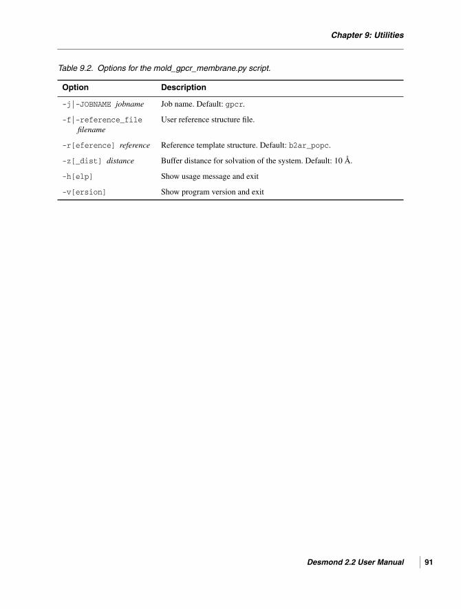
Chapter 9: Utilities
Table 9.2. Options for the mold_gpcr_membrane.py script.
Option Description
-j|-JOBNAME jobname Job name. Default: gpcr.
-f|-reference_filefilename
User reference structure file.
-r[eference] reference Reference template structure. Default: b2ar_popc.
-z[_dist] distance Buffer distance for solvation of the system. Default: 10 Å.
-h[elp] Show usage message and exit
-v[ersion] Show program version and exit
Desmond 2.2 User Manual 91

92
Desmond 2.2 User Manual
Desmond User Manual
Appendix A
Appendix A: Creating a CMS File from a Full SystemMaestro File
If you have a Maestro file that contains the entire system, including solvent, you can generate aCMS file that can be used in Desmond using the System Builder. The procedure given below isuseful when you have a system that was generated by another application.
First, if the property s_ffio_ct_type is present, you must edit the Maestro file and removeit.
To create a CMS file using the System Builder panel:
1. Import the system into Maestro.
2. From the Applications menu, choose Desmond, then System Builder.
3. Set the Solvent model to None.
4. Select the appropriate box shape.
5. Specify the box size in one of the following ways:
• Set the Box size calculation method to Absolute size and type in the box dimensions.
• Set the Box size calculation method to Buffer and enter 0.0 for the buffer distances.This approach will not give the exact box size for the input structure. However itwill work reasonably well, particularly when the exact box size is not known.
6. Click Start.
7. Enter a job name and click Start.
The output CMS file is named jobname-out.cms.
To create a CMS file from the command line:
1. Edit the Maestro file and add the properties that specify the box shape with the appropri-ate values. The properties are:
r_chorus_box_ax, r_chorus_box_ay, r_chorus_box_az,r_chorus_box_bx, r_chorus_box_by, r_chorus_box_bz,r_chorus_box_cx, r_chorus_box_cy, r_chorus_box_cz
2. Create a CSB file, my-build.csb that has the following content:
{read_solute_structure input-file.mae
Desmond 2.2 User Manual 93

Appendix A: Creating a CMS File from a Full System Maestro File
94
create_boundary_conditions cubic 0.000000write_maeff_file output-file.cms}
3. Run the System Builder with the following command:
$SCHRODINGER/utilities/system_builder my-build.csb
The CMS file that is generated is named output-file.cms.
Desmond 2.2 User Manual

Desmond User Manual
Appendix B
Appendix B: The multisim Utility
The multisim utility is useful for running tasks that consist of a sequence of steps, such asrelaxation of a system followed by a production simulation. Maestro runs multisim for jobsthat include multiple stages. This appendix provides detailed information on how to runmultisim and the format of multisim (.msj) files.
Multisim is used by both Desmond and MCPRO+ for running jobs.
B.1 Running multisim
The basic usage information for multisim, including examples, is given in Section 6.2 onpage 62. This section describes more advanced multisim features such as templatemultisim commands, node locking, restarting multisim jobs, and obtaining informationfrom multisim checkpoint files.
B.1.1 Template multisim Commands
Most .msj files produced by Maestro end with a commented out example of the commandneeded to run the job. For example
$SCHRODINGER/utilities/multisim -JOBNAME example -HOST master_job_host-host subjob_host -maxjob 0 -cpu "2 2 2" -i example.cms -m example.msj-cfg example.cfg -o example-out.cms
To use this command you would replace the following text with the values for your own setup:
• master_job_host—the host on which to run the master job (the Python script thatmanages the multisim job).
• subjob_host—the host on which to run the subjobs, which are often cpu intensive.
• example—the job name and the stem of various file names, which are constructed in astandard way from the job name.
• the cpu specification "2 2 2"—the specification of the CPUs used by the job. This spec-ification can either be a triplet of numbers that defines the spatial decomposition of thesystem, with the total number of processors being the product of these three numbers; ora single integer, which is the total number of processors, and must have only the factors 2,3 and 5.
Desmond 2.2 User Manual 95

Appendix B: The multisim Utility
96
• the value for -maxjob, which is used to specify how many subjobs can be queued at thesame time for FEP jobs. The value 0 means “all subjobs”.
B.1.2 Node Locking
Node locking involves requiring all subjobs to run on the same nodes (CPUs) as the master job.Node locking can be turned on by adding -mode umbrella to the command line. This featurecan be useful on busy computer systems that are controlled by a queuing system, because onlythe master process is submitted to the queuing system. All subjobs will then run on the nodesallocated to the master process without being resubmitted to the queuing system. When thisoption is given the -host option is ignored.
Node locking is not supported for FEP jobs.
B.1.3 Restarting multisim Jobs
The multisim job periodically writes out a checkpoint file, which records the current state ofthe workflow. The checkpoint file is named jobname-multisim_checkpoint. This file doesnot include data produced by subjobs. The checkpoint file is copied back to the job launchdirectory when the master job stops.
In most cases the multisim job can be restarted with a command similar to the following:
$SCHRODINGER/utilities/multisim -r myjob-multisim_checkpoint-d myjob_stage-out.tgz -JOBNAME myjob
where you specify the checkpoint file with the -r option and the -out.tgz file of the lastcompleted stage with the -d option. The -d option is usually necessary because the subsequentstages need access to the data produced by the last successfully completed stage. For example,if stage 5 is partially done (some subjobs finished, some did not), then you would also have toinclude myjob_4-out.tgz, and the command to use would be:
$SCHRODINGER/utilities/multisim -r myjob-multisim_checkpoint-d myjob_5-out.tgz -d myjob_4-out.tgz -JOBNAME myjob
This command restarts the job on the same compute hosts as before. Unless the -HOST optionis given the master job runs on the local host. The subjobs will run using the same number ofCPUs as before. If you want to use different hosts to restart a job you can use the -HOST and–host options. The number of CPUs used by the subjobs can also be changed using the -cpuoption, for example,
$SCHRODINGER/utilities/multisim -HOST another_master_host-host another_subjob_host -r myjob-multisim_checkpoint-d myjob_5-out.tgz -JOBNAME myjob -cpu 1
Desmond 2.2 User Manual

Appendix B: The multisim Utility
You can also modify the characteristics of some stages when you restart a job, by using the–set option. For example, if you use the command:
$SCHRODINGER/utilities/multisim -r myjob-multisim_checkpoint-d myjob_4-out.tgz -JOBNAME myjob-set "stage[5].time = 1200.0 stage[5].cutoff_radius = 16.0"
then stage 5 is modified so that its subjobs run with the time set to 1200.0, and thecutoff_radius set to 16.0. However, if you also provide the stage 5 .tgz file and some subjobsfrom stage 5 have finished, only the unfinished jobs will run with the new settings.
You can also restart a job with a different .msj file. For instance, the command:
$SCHRODINGER/utilities/multisim -r myjob-multisim_checkpoint-d myjob_5-out.tgz -JOBNAME myjob -m newworkflow.msj
runs the uncompleted stages according to newworkflow.msj. This new .msj file mustcontain the same completed stages as the original job. Any of the remaining stages can bemodified or deleted, and new stages may be inserted.
Some other changes that you can or cannot make are:
• You can restart the job with a different .cfg file by specifying the new .cfg file with the-cfg option.
• You can restart the job with a different maximum number of simultaneously running sub-jobs by using the -maxjob option.
• You cannot change the node-locking mode.
In most cases, multisim automatically detects and uses additional input files needed for a jobwhen it is restarted. If the job fails because an existing input file was not detected whenrestarting a job you can specify that file by using the -ADD_FILE option.
B.1.4 Obtaining Information from multisim Checkpoint Files
To obtain information on the contents of a multisim_checkpoint file, you can use themultisim command with the -probe option:
$SCHRODINGER/utilities/multisim -probe myjob-multisim_checkpoint
This command summarizes the contents of the checkpoint file without submitting a job tocontinue the calculation. Below is an example of the output from a successful relative solvationfree energy calculation:
Probing checkpoint file: Benzene-to-Pyridine_solvent-multisim_checkpoint multisim version: 3.2
Desmond 2.2 User Manual 97

Appendix B: The multisim Utility
98
mmshare version: 18104 Jobname: Benzene-to-Pyridine_solvent Username: me Master job host: tabitha.schrodinger.com Subjob host: myhost CPUs per subjob: "1" Original start time: Sat May 2 00:26:20 2009 Checkpoint time: Sat May 2 02:34:16 2009 Master job ID: tabitha-0-49fbcb67 Structure input file: /scr/me/Benzene-to-Pyridine_lig.mae Original *.msj file: /scr/me/Benzene-to-Pyridine_solvent.msj
Stages: Stage 1 completed. Stage 2 completed. Stage 3 completed. Stage 4 completed. Stage 5 completed. Stage 6 completed.
If the job had failed in Stage 5 you would see something like:
...Stage 5 partially completed. 1 subjobs failed, 11 subjobs done.
Jobname of failed subjobs: Benzene-to-Pyridine_5_lambda2 Stage 6 not run.
To resume the job as described earlier, this output tells you that you need to provide the .tgzfile from stage 4, and that you might want to provide the .tgz file from the partially completedstage 5. In this case only one subjob failed in stage 5 so rerunning just that subjob mightrequire significantly less computer time than rerunning the entire stage.
B.2 The multisim File Syntax
The multisim input file (.msj file) generally adheres to the Ark format from D. E. ShawResearch. This is the same syntax that is used in Desmond configuration (.cfg) files, whichare described in brief in Appendix C and in full in the Desmond User’s Guide. Ark format iscompletely compatible with the syntax used in multisim files in Schrödinger Suite 2008, butsupports other features.
The syntax rules of the Ark format can be summarized as follows.
• Values are assigned to a keyword with the keyword = value syntax.
• Values can be numbers, strings, lists, or blocks. Numbers can be integers or real numbers.Strings do not need to be enclosed in quotes unless they contain embedded blanks.
Desmond 2.2 User Manual

Appendix B: The multisim Utility
• A block is one or more settings within a pair of braces, { }. For example: a = { b = 3c = 4 }. The block in this example contains two keyword-value assignments.
• A list is a sequence values that is enclosed by a pair of square brackets [ ]. Elements of alist do not have to be of the same type. An example is [ 1 { a = 1 } 5 [ 2 3 ] ].
• Hierarchical expressions involving blocks and lists can be created: there is no limit onnesting of lists and blocks.
• Individual elements of a hierarchy can be set by joining the names of the parents withperiods to form a compound key. For example, a.b.c = 3 sets element c of block b inblock a to 3.
• If a keyword is assigned a value twice, the second takes precedence. If the value is ablock the blocks are merged and keywords present in each block are assigned the valuesfrom the latter block.
• The = sign can be omitted if the value is a block value. This means that a = { b = 1 }and a { b = 1 } are equivalent. This syntax is used to specify the multisim stages.
Multisim processing deviates from the Ark standard in the following ways:
• Multisim stages with the same name remain separate, otherwise stages that appear morethan once in an .msj file (such as simulate or minimize) would be combined into onestage.
The multisim input file consists of a sequence of stages, each of which specifies a particularcalculation to be run. Each stage has its own distinct data structure. A stage begins with a labelidentifying the type of stage followed by braces enclosing parameters for that stage. A msj filewill in general look something like:
#an outline for a msj file.first_stage_name { parameter1 = 3000.0 parameter2 = "this is a string" parameter3 = [ "list element 1" 2 "list element 3" ]}second_stage_name{
parameter5 = 20}
The types of stages that are supported for Desmond include the following:
• task—describes the type of job• minimize—minimize the system
Desmond 2.2 User Manual 99

Appendix B: The multisim Utility
100
• simulate—run an MD simulation on the system• system_builder—run the system builder• replica_exchange—run a replica exchange MD simulation on the system• solvate_pocket—add or remove water molecules in buried pockets.• fep_analysis—analyze FEP calculations• extern—custom Python stage
The keywords supported for each of these stages and their default values are described in thesections that follow.
B.2.1 General Keywords
The keywords that can be used in any stage of the multisim job are listed in Table B.1.
B.2.2 Desmond-Specific Common Keywords
The stages that run Desmond directly (minimize, replica_exchange, and simulate)accept a common set of keywords in addition to keywords specific to the Desmond task.
Table B.1. General keywords that can be used in any stage.
Keyword Description
compress File name pattern of the stage data file. If it is set to an empty string, then thedata of this stage is not packaged and compressed. Default:$JOBNAME_$STAGENO-out.tgz.
dir Pattern for the names of the directories used by subjobs of this stage. Default:[$JOBPREFIX/][$PREFIX/]$JOBNAME_$STAGENO[_lambda$LAMBDA]
jobname Jobname pattern for subjobs of this stage. Default:$JOBNAME_$STAGENO[_lambda$LAMBDA]
prefix Value of the PREFIX macro, which by default is used to specify the sub-direc-tory name of subjobs (see the dir keyword). Default is an empty string.
should_skip Skip this stage. Allowed values: true, false. Default: false.
should_sync Do not start this stage until all subjobs of the previous stage finish successfully.Allowed values: true, false. If it is set to false, this stage is started as soon asany subjob of the previous stage finishes successfully. For FEP jobs, setting thiskeyword to false can result in earlier completion of the job. Default: true.
struct_output File name of the final output structure file. This keyword is only effective whenset in the last stage, and the setting can be overwritten by the -o option ofmultisim.
title The title for the stage. Default: no title.
Desmond 2.2 User Manual

Appendix B: The multisim Utility
Keywords for the config file, the interaction and setting the number of CPUs are listed inTable B.2.
B.2.3 The restrain Keyword
The restrain keyword specifies the atom sets to be restrained. Restraints set in all stagesexcept the system_builder stage apply only to the current stage. Restraints set in thesystem_builder stage are “permanent”—they are inherited by all subsequent stages. Perma-nent restraints can be overridden in a particular stage, but only to increase the restraint forceconstants. They will still be applied in subsequent stages.
The restrain keyword supports the specific values listed in Table B.3, and also supports ablock syntax and a list syntax.
Restraints can be specified using blocks, and ASL expressions can be used to define the atomsthat are restrained within restraint blocks. The syntax is:
restrain = {atom = atoms force_constant = valuereference_position = retain|reset }
where atoms can be solute, solvent, solute_heavy_atom, or heavy_atom as before, oran ASL expression prefixed by asl:. For example,
restrain = {atom = asl:all force constant = 10}
Table B.2. Keywords for Desmond-specific stages.
Keyword Description
cfg_file Config file (.cfg) that provides the default values for simulation. Thisoption is not required and is usually used to customize simulationsbeyond the keywords supported by multisim.
cfg_overwrite Settings to override the values given in the config file. Specifies a blockin Ark syntax that contains the desired settings.
cutoff_radius Cutoff radius for the short-range interactions in angstroms. Default: 9 Å.
coulomb_method Long-range Coulomb interaction treatment. Allowed values are pme(use smooth particle mesh Ewald), cutoff (use cutoff only).Default: pme.
cpu Number of processors to use and optional topology. If given as a singleinteger, the topology is determined automatically. To specify the topol-ogy, use the format [n1 n2 n3] or "n1 n2 n3". For replica exchange,this keyword specifies the processors to use for each replica.Default: [2 2 2].
Desmond 2.2 User Manual 101

Appendix B: The multisim Utility
102
restrains all atoms with a force constant of 10 kcal mol-1 Å-2. Restraints can be applied withrespect to the positions of the atoms at the start of the current stage by settingreference_position to reset or the positions from the previous stage by settingreference_position to retain. The default is reference_position=reset.
Different groups of atoms in the system can be restrained with different force constants bylisting the restraint blocks for each set of atoms within a list using the syntax:
restrain = [{atom = "asl:ASL1" force_constant = value1}{atom = "asl:ASL2" force_constant = value2} ... ]
If the ASL expression contains quotes, they must be escaped, either by using a backslash, or byusing double quotes in the ASL expression and surrounding the entire expression in singlequotes.
B.2.4 The atom_group Keyword
The atom_group keyword can be used to define atoms groups within the .cms file. Atomgroups can be frozen, restrained or associated with particular thermostats. The atom group isdefined by the atom-level property i_ffio_grp_name. This keyword can be set to thefollowing values:
• none—Remove all atom groups.
• retain—Keep all atom groups from the previous stage.
• { atom = atoms index = i name = name }—atom group block. Put the specifiedatoms in the atom group i that has the name name. The atom keyword accepts the same
Table B.3. Specific allowed values of the restrain keyword.
Value Description
heavy_atom restrain all heavy (non-hydrogen) atoms
none Remove the temporary restraints (those set in the previous simulate orminimize stage), but do not change permanent restraints such as those setin the system_builder stage or present in the original .cms file given tothe multisim job. If you use this value in a system_builder stage, itremoves all restraints. This is the default.
retain Keep the restraints as set in the previous stage.
solute Restrain all solute atoms
solute_heavy_atom Restrain all heavy atoms in the solute
solvent Restrain all solvent atoms
Desmond 2.2 User Manual

Appendix B: The multisim Utility
values for atoms as the atom keyword for restrain, described above. The index i is thevalue for the i_ffio_grp_name property. Desmond only supports index numbers from0 to 7.
• [ group1 group2 ... ]—Specify multiple atom groups. Each group can be specified asa block, in the above format.
An atom group set in the system_builder stage is persistent, which means that it remainsdefined in all subsequent stages, until the next system_builder stage.
B.2.5 The task Stage
The .msj file should start with a task stage to specify the type of job. Although Multisim candetermine the type of job based on the input structure file provided, this can lead to unpredict-able behavior if the file was previously used by a different type of job. Explicitly stating the jobtype avoids this problem, and also permits Multisim to ensure that the input structure fileprovided is appropriate for the type of calculation requested.
If the first stage is not a task stage, Multisim inserts a task stage and issues a warning. Theinserted task stage has the task parameter set to desmond:auto or mcpro:auto.
The task stage has only one keyword, task, whose allowed values are listed in Table B.4.
B.2.6 The system_builder Stage
Keywords for the system_builder stage are listed in Table B.5. The keywords restrain(Section B.2.3 on page 101) and atom_group (Section B.2.4 on page 102) can also be used inthis stage. When they are used, the settings are persistent: they apply to all subsequent stagesunless explicitly overridden by another system_builder stage.
Table B.4. Values of the task keyword.
Value Description
desmond:regular Non-FEP Desmond job
desmond:fep Desmond absolute or relative free energy (FEP) job
desmond:afep Desmond absolute free energy (FEP) job
desmond:auto Desmond job whose type is determined from the input structure file
mcpro:auto MCPRO+ job whose type is determined from the input structure file
mcpro:fep MCPRO+ FEP job
Desmond 2.2 User Manual 103

Appendix B: The multisim Utility
104
B.2.7 The simulate and replica_exchange Stages
The keywords that are specific to the simulate and the replica_exchange stages are listedin Table B.6. The keywords restrain (Section B.2.3 on page 101) and atom_group(Section B.2.4 on page 102) can also be used in this stage. When they are used, the settings aretemporary: they apply only to the current stage.
Table B.5. Keywords for the system_builder stage.
Keyword Description
csb_file Input composite system builder (.csb) file. This option is notrequired and is usually used to customize system building beyondthe keywords supported by multisim.
solvate_system Solvate the system. Allowed values are true, false.Default: true.
neutralize_system Add counter ions to neutralize the system. Allowed values aretrue, false. Default: true.
buffer_width Minimum distance between the box edge and solute in Ang-stroms. Default: 10.0 Å.
rezero_system Reset the original of the coordinates to the center of mass of thesolutes. Allowed values are true, false. Default: true.
box_shape Specifies the box shape. Allowed values are cubic,orthorhomibic, triclinic. Default: cubic.
solvent Solvent type.Allowed values are SPC, TIP3P, TIP4P, andTIP4PEW. Default: SPC.
Table B.6. Keywords for the simulate stage.
Keyword Description
barostat_relaxation Relaxation time constant for barostat in picoseconds.Default: 2.0 ps.
coulomb_method Coulomb interactions. Allowed values are pme, cutoff.Default: pme.
ensemble Specifies the ensemble to be used for the simulation. Allowed val-ues are NPT, NPT_Ber, NVT, NVT_Ber, NVE. Default: NPT.
jin_file List of auxiliary input files for the stage. Usually only needed whencustom plugins are used.
jout List of auxiliary output files for the stage. Usually only neededwhen custom plugins are used.
Desmond 2.2 User Manual

Appendix B: The multisim Utility
B.2.8 The minimize Stage
The keywords that are specific to the minimize stage are listed in Table B.7. The keywordrestrain (Section B.2.3 on page 101) can also be used in this stage. When it is used, thesettings are temporary: they apply only to the current stage.
pressure Pressure for the simulation in bars. Default: 1.01325 bar.
rand_initial_velocities Random number used to generate the initial velocities. Set to 0 touse velocities from input .cms file. Default: 2007.
resampling_period Frequency of resampling in picoseconds.
temperature Temperature for the simulation in kelvin. For replica exchange, thismust be a list of temperatures, one for each replica. Default: 300 K.
thermostat_relaxation Relaxation time constant for thermostat in picoseconds.Default: 1.0 ps.
time Simulation time in picoseconds. Default: 1200 ps.
timestep RESPA bonded, near, and far time steps in ps, provided as a stringor a list. Default: "2 2 6" or [2 2 6].
Table B.7. Keywords for the minimize stage.
Keyword Description
max_steps Maximum iterations. Default: 200.
convergence Convergence threshold in kcal/mol/Å. Default: 1.0 kcal/mol/Å.
steepest_descent_steps Number of steepest descent steps performed before switching to theLBFGS algorithm. Default: 10.
Table B.6. Keywords for the simulate stage. (Continued)
Keyword Description
Desmond 2.2 User Manual 105

Appendix B: The multisim Utility
106
B.2.9 The solvate_pocket Stage
The keywords for the solvate_pocket stage are listed in Table B.8. This stage runs thesolvate_pocket utitlity, which is described in Section 9.1 on page 85.
Table B.8. Keywords for the solvate_pocket stage
Keyword Description
spd_file The name of the solvate_pocket command file. If omitted, the defaultsettings are used.
spd_overwrite Block that provides settings in Ark syntax to overwrite specific commandsin the command file. All keywords other than spd_file andligand_file must be inside this block.
ligand_file The name of the ligand file used to define the region sampled. If the nameis set to an empty string or omitted, the name jobname-ligand.mae isused. A ligand must be used to define the region.
name A descriptive name for the simulation. Default: name of standardsolvate_pocket command file.
temperature The temperature used in the Monte Carlo simualtion. Default: 300 K
init_num_passes The number of Monte Carlo passes to perform in the equilibration prior tothe production Monte Carlo run. Default: 10000.
num_passes The number of Monte Carlo passes to perform in the production MonteCarlo run. Default: 100000.
update_frequency The number of passes between updates in the log file. Default: 100.
pass_term_window The number of passes over which the slope of the standard deviation of thethe number of water molecules is calculated. This keyword may be used toterminate the calculations before the number of passes specified bynum_passes has been completed. The simulation portions will run for atleast twice this duration before early termination occurs. Default: 100000.
term_std_slope Threshold for the standard deviation of the number of water molecules.The calculation is terminated if the standard deviation falls below thisvalue. Default: 0.00001.
num_trans_rot The number of water molecule translations to attempt per pass. Thisshould be set to approximately the number of water molecules expected toreside in the region being sampled. Default: 100.
num_delete The number of attempts to delete a single water molecule per pass.Default: 25.
num_insert The number of attempts to insert a single water molecule per pass.Default: 25.
Desmond 2.2 User Manual

Appendix B: The multisim Utility
B.2.10 The extern Stage
The extern stage provides an extremely flexible way to include your own Python code in amultisim run. The code can be embedded in the .msj file as a string value assigned to thecommand keyword. For example:
extern { command = "import os;def main( current_stage, job ): os.system( ’ls’ )"}
In the embedded Python code, you can import and use modules from your Schrödinger Pythoninstallation. If you need extra modules, you can pass their file names to multisim by settingthe auxiliary_file parameter, and multisim transfers them to the scratch directory of themaster job at run time. For example:
extern { auxiliary_file = [mod1.py mod2.py] command = "import osimport mod1import mod2def main( current_stage, job ): // does something with mod1 and mod2
max_disp The maximum change used in each of the x, y, and z directions for a com-bined translation/rotation move. Default: 0.105 Å.
max_dpsi The maximum change used for phi and psi (Euler angles) in radians for acombined translation/rotation move. Default: 0.318.
max_dctheta The maximum change used for the cosine of theta (Euler angle) for a com-bined translation/rotation move, in radians. Default: 0.0654.
cut_off The cutoff distance for calculating electrostatic and Lennard-Jones inter-actions. Default: 9.0 Å.
short_dist The closest acceptable approach for any two atoms. Default: 1.0 Å.
chemical_potential The chemical potential of water in kcal/mol. Default: -7.17 kcal/mol (forTIP4P).
Table B.8. Keywords for the solvate_pocket stage
Keyword Description
Desmond 2.2 User Manual 107

Appendix B: The multisim Utility
108
os.system( ’ls’ )"}
The code given above is run once for each subjob in the previous stage. If you want to run itonly once, use command_once instead of command. For example:
extern { auxiliary_file = [mod1.py mod2.py] command_once = "import osimport mod1import mod2def main( current_stage ): // does something with mod1 and mod2 os.system( ’ls’ )"}
For scripts that are stage-specific, your code must provide a main function that takes two argu-ments for command or one for command_once. The first argument in both cases correspondsto information for the current stage, while the second argument for command corresponds toinformation from the previous stage.
For very simple scripts, your code for command or command_once does not need to provide amain function. The following example removes a temporary file if it exists:
extern { command = "import os# Removes a temporary file.if (os.path.isfile( ’my_temporary_file’ )) : os.remove( ’my_temporary_file’ )"}
Without the main function, multisim cannot pass the current stage and the current job objectsto the Python code, but that is presumed to be not needed for simple operations.
The extern stage is an advanced feature. Please do not hesitate to contact us for addition infor-mation on its use. The keywords for this stage are listed in Table B.9.
Desmond 2.2 User Manual

Appendix B: The multisim Utility
B.2.11 The fep_analysis Stage
Keywords for the fep_analysis stage are listed in Table B.10.
Table B.9. Keywords for the extern stage.
Keyword Description
auxiliary_file List of files containing extra modlues to be transferred to the runtime direc-tory.
command Command to execute once for each subjob of the previous stage. The com-mand specifies Python code that can span multiple lines.
command_once Command to execute once for the previous stage. The command specifiesPython code that can span multiple lines.
Table B.10. Keywords for the fep_analysis stage.
Keywords Description
bennett.random_seed Random seed for the Bennett method. Default: 2111839.
correct_vdw Calculate the long range dispersion correction for absolute free energyjobs. This keyword has no effect for relative free energy jobs. Default:true.
correct_restr Calculate the enthalpic correction for position restraints. This parameterdoes no harm if the production simulations have no restraints. Default:true.
Desmond 2.2 User Manual 109

110
Desmond 2.2 User Manual
Desmond User Manual
Appendix C
Appendix C: The Desmond Configuration File
C.1 General Structure
Desmond configuration files (“config files” for short) adhere to the Ark format from D. E.Shaw Research, and have the extension .cfg. The definitive description of this format is avail-able in the Desmond User’s Guide. This format is also used by multisim (.msj) files.
Config files are composed of a number of sections that are usually delimited with the followingstatement:
section-name = { section-contents }
In general section-contents consists of a number of keyword = value statements. The concept ofvalues includes not only a number or a string but also a block or a list. A block is one or moresettings within a pair of braces, { }. For example:
a = { b = 3 c = 4}
where a is set to the block value { b = 3 c = 4 } that contains two settings. A list is asequence of values that is enclosed by a pair of square brackets [ ]. For example:
a = [ 3 5 ]
where a is set to a list [ 3 5 ] that contains two values. Elements of a list do not have to be ofthe same type. Here are some examples of valid lists:
Hierarchical expressions involving blocks and lists help elucidate the relationships within thedata. You can also set the values of variables within a hierarchy without reference to the wholedata structure. For example,
a = { b = 3 c = 4 }
can be written as:
a.b = 3 a.c = 4
[ 1 string 5 ] a list consisting of an integer, a string and an integer.
[ 1 { a = 1 } 5 ] a list consisting of an integer, the block { a = 1 } and anotherinteger
[ [ 1 2 ] 1 3 ] a list consisting of the list [ 1 2 ] followed by two integers.
Desmond 2.2 User Manual 111

Appendix C: The Desmond Configuration File
112
The Ark standard specifies that if the same parameter is assigned two different values thesecond one will be used. If the value is a block the blocks are merged and parameters present ineach block are assigned the values from the latter block.
The = symbol can be omitted if the value is a block value. This means that
a = { b = 1 }
and
a { b = 1 }
are equivalent.
Lines starting with a # character are treated as comments.
C.2 Units
The units used in the configuration file are:
• time: ps• distance: angstroms• energy: kcal/mol• pressure: bar• surface tension: bar angstroms• temperature: kelvin
Boolean values must be set to either true or false. Time can be specified as a positive realnumber or as the string inf, meaning infinity, or “never”.
C.3 Configuration File Sections
Table C.1 lists the supported top-level sections for the configuration file. These sections aredescribed in the document sections and tables below.
Table C.1. Top-level sections.
Section Name Description Job Type
boot Sets parameters for booting the backend all
constraint Sets parameters for contraints all
Desmond Provides general information about Desmond all
force Sets parameters related to interactions amongst the atoms all
Desmond 2.2 User Manual

Appendix C: The Desmond Configuration File
C.3.1 The boot Section
The boot section contains a single keyword, file, which specifies the name of the input .cmsfile. This keyword is overwritten by the Desmond driver script.
C.3.2 The constraint Section
The keywords for the constraint section are listed in Table C.2.
C.3.3 The Desmond Section
The Desmond section contains a single keyword, config_version, which gives the configfile format version.
global_cell Provides information for domain decomposition all
integrator Sets parameters for integrating the equations of motion simulation incl.REMD
mdsim Sets parameters for simulations (e.g. duration) simulation
minimize Sets parameters for minimizations (e.g. number of steps) minimization
remd Sets parameters for replica exchange molecular dynamics(REMD) simulations
REMD simula-tion
vrun Sets parameters for analysis runs analysis
Table C.2. Keywords for the constraint section.
Keyword Description
tol Convergence tolerance. Default: 1e-8
maxit Maximum number of iterations. Default: 8.
Table C.1. Top-level sections. (Continued)
Section Name Description Job Type
Desmond 2.2 User Manual 113

Appendix C: The Desmond Configuration File
114
C.3.4 The force Section
The keywords for the force section are listed in Table C.3. This section contains subsections,whose keywords are described in Table C.4–Table C.7.
Table C.3. Keywords for the force section.
Keyword Description
Required
type Type of routine for calculating forces. Allowed values: desmond,gibbs. Use gibbs for FEP simulations.
nonbonded Section for nonbonded settings
Optional
average_dispersion Used to calculate energy and virial corrections due to cutoff. Example:69.5
bonded_terms The set of bonded terms [stretch angle dihedral improper pair cmap]
gibbs Section for setting up FEP simulations
global_forces Only available as BiasingForce
Table C.4. Keywords for the force.nonbonded section.
Keyword Description
elec Functional form of the electrostatic interactions. Allowed values: ewald, cutoff.Must be set to cutoff if force.nonbonded.far.type is none.Default: ewald.
type Functional form for pairwise nonbonded interaction. Allowed values: vdw-elec,none.
r_lazy Pair list assembly cutoff radius
r_cut Pairwise interaction cutoff distance
n_zone Number of interpolation zones (points in tabular versions of the potentials).Default: 1024.
far Section describing implementation of far-field interaction
Desmond 2.2 User Manual

Appendix C: The Desmond Configuration File
For the force.gibbs.lambda section, the schedules are lists of lambda values, e.g.
[ 0.0 0.14 0.28 0.42 0.57 0.71 0.85 1.0 1.0 1.0 1.0 1.0 ]
All lists in this section must be of the same length or empty.
Table C.5. Keywords for the force.nonbonded.far section.
Keyword Description
type Far-field interaction type. Example: pme
sigma Ewald sigma coefficient
n_k FFT grid size. The value on each axis may only have 2, 3, and 5 as factors and isrelated to the partition setting in the global_cell section (Table C.8) .Example: [64 64 64]
order PME interpolation order; 4-7
sigma_s sigma if type = gse
r_spread spread of type = gse
Table C.6. Keywords for the force.gibbs section.
Keyword Description
fec_type Free energy calculation type. Allowed values are:none—alchemical—use for relative FEPligand_binding—use for absolute FEP
alpha_vdw Alpha parameter in the soft core potential
i_window FEP window index
lambda Section for setting up lambda schedule
Table C.7. Keywords for the force.gibbs.lambda section.
Keyword Description
vdw Van der waals schedule for absolute FEP. Must be set to [ ] for relative FEP.
coulomb Coulomb schedule for absolute FEP. Must be set to [ ] for relative FEP.
vdwA Vdw schedule of initial structure for relative free energy. Must be set to [ ]for absolute FEP.
vdwB Vdw schedule of final structure for relative free energy. Must be set to [ ]for absolute FEP.
Desmond 2.2 User Manual 115

Appendix C: The Desmond Configuration File
116
C.3.5 The global_cell Section
The keywords for the global_cell section are listed in Table C.8.
chargeA Charge schedule of initial structure for relative free energy. Must be set to[ ] for absolute FEP.
chargeB Charge schedule of final structure for relative free energy. Must be set to [ ]for absolute FEP.
bondedA Bonded terms schedule of initial structure for relative free energy. Must be setto [ ] for absolute FEP.
bondedB Bonded terms schedule of final structure for relative free energy. Must be setto [ ] for absolute FEP.
output.name Name of the FEP data file. Example: fep.dE.
output.first Simulation time to start writing FEP data
output.interval Simulation time interval for writing FEP data
Table C.8. Keywords for the global_cell section.
Keyword Description
Required keywords:
n_replica Number of replicas. Should be set to 1 except for replica exchange.
partition Grid dimensions for the home boxes. The simulation box is divided intosmaller boxes by partitioning the system in the a, b, and c directions fordomain decomposition parallelization. The number of partitions on eachaxis must have only 2, 3, and 5 as factors, and must also divide evenlyinto the FFT grid size, n_k (see Table C.5). Example: [4 4 4].
r_clone Clone buffer radius. Example: 5.3125
reference_time Constant offset added to elapsed chemical time during simulation
Optional keywords:
clone_policy Allowed values: rounded, unrounded. In most situations rounded ispreferred
est_n_atom_per_voxel Estimated number of atoms per particle array voxel
est_p_dens Estimated required size of Desmond communication buffers
Table C.7. Keywords for the force.gibbs.lambda section.
Keyword Description
Desmond 2.2 User Manual

Appendix C: The Desmond Configuration File
C.3.6 The integrator Section
The keywords for the integrator section are listed in Table C.9. Keywords for sections withinthis section are listed in the following tables.
Table C.9. Keywords for the integrator section.
Keyword Description
center_frozen_group Keep frozen atoms centered. Allowed values: true, false.Default: true.
dt Innermost RESPA time step in fs.
isotropy Type of global cell changes permitted. Allowed values:isotropic, semi_isotropic, anisotropic,constant_area.
max_margin_contraction Used to maintain the integrity of PNE calculation
migrate Section describing migration.
p_ref Reference pressure
pressure Barostat section.
remove_com_motion Remove center of mass motion of the whole system. Allowed val-ues: true, false. You should set this keyword to true forBer_NVT and Ber_NPT, and to false otherwise. Default: false.
respa Section describing updates for RESPA.
temperature Thermostat section, one list per thermostat. Example:temperature = [{T_ref = 300 groups=[1]}{T_ref=100 groups=[2]}]
type Type of integrator and associated ensemble. Allowed values:V_NVE, NH_NVT, MTK_NPT, Ber_NVT, Ber_NPT, L_NVT, L_NPT,Piston_NPH, and anneal. For each integrator type there is anassociated section that provides additional information.
Optional
anneal Simulated annealing section. This section has the same keywordsas its parent, integrator, except that the type cannot be set toanneal, and it cannot contain an anneal section.
tension_ref Specifiy the surface tension for constant surface tension simula-tions. Default: 0.
V_NVE Constant-energy dynamics, no available options
Desmond 2.2 User Manual 117

Appendix C: The Desmond Configuration File
118
NH_NVT Nose-Hoover NVT dynamics section. Contains only thethermostat section described in Table C.13.
MTK_NPT Martyna-Tobias-Klein NPT dynamics section. Contains only thethermostat section described in Table C.13 and the barostatsection described in Table C.14.
Ber_NVT Berendsen NVT dynamics section. Contains only the thermostatsection described in Table C.15.
Ber_NPT Berendsen NPT dynamics section. Contains only the thermostatsection described in Table C.15 and the barostat sectiondescribed in Table C.16.
L_NVT Langevin NVT dynamics section. Contains only the thermostatsection described in Table C.17.
L_NPT Langevin NPT dynamics section. Contains only the thermostatsection described in Table C.17 and the barostat sectiondescribed in Table C.14.
Piston_NPH Constant-enthalpy dynamics section. Contains only the barostatsection described in Table C.14.
Table C.10. Keywords for the integrator.migrate section
Keyword Description
first First migration time. May be overridden automatically. Default: 0.0.
interval Time between migrations. May be overridden automatically. Default: 0.012.
Table C.11. Keywords for the integrator.respa section
Keyword Description
bonded_interval Steps between bonded force updates. Default: 1.
nonbonded_near_interval Steps between nonbonded force updates. Default: 1.
nonbonded_far_interval Steps between far field force updates. Default: 3.
Table C.9. Keywords for the integrator section. (Continued)
Keyword Description
Desmond 2.2 User Manual

Appendix C: The Desmond Configuration File
Several of the integrators have common thermostat and barostat sections. The keywords forthese sections are listed in Table C.13 and Table C.14. Keywords for other integrator sectionsare listed in the remaining tables of this section.
Table C.12. Keywords for the integrator.temperature section
Keyword Description
T_ref Reference temperature. Default: 300.0 K.
groups List of temperature groups assigned to thermostat. Default: 0, meaning the entiresystem.
Table C.13. Keywords for the common thermostat section.
Keyword Description
mts Time steps within chain. Default: 2.
tau Relaxation time for chain members. Example: [1. 1. 1.]
Table C.14. Keywords for the common barostat section.
Keyword Description
tau Barostat relaxation time. Default: 2.0.
T_ref Barostat temperature. Default: 300.0 K.
thermostat Thermostat section for the barostat. This is the section described in Table C.17 forthe L_NPT barostat, and is the common section described in Table C.13 for otherbarostats. Not used for the Piston_NPH integrator.
Table C.15. Keywords for the Ber_NPT and Ber_NVT sections.
Keyword Description
barostat Barostat section (Ber_NPT only)
tau Temperature relaxation time; one per thermostat. Default: [1.0].
min_velocity_scaling Lower bound for velocity scaling. Default: 0.85.
max_velocity_scaling Upper bound for velocity scaling. Default: 1.20.
Desmond 2.2 User Manual 119

Appendix C: The Desmond Configuration File
120
C.3.7 The mdsim Section
The keywords for the mdsim section are listed in Table C.18. This section has one subsection,whose keywords are listed in Table C.19.
Table C.16. Keywords for the Ber_NPT barostat section
Keyword Description
tau Pressure relaxation time. Default: 2.0.
kappa Compressibility. Default: 4.5e-5.
min_contraction_per_step Lower bound for home box rescaling. Default: 0.95.
max_contraction_per_step Upper bound for home box rescaling. Default: 1.10.
Table C.17. Keywords for the L_NVT and L_NPT thermostat sections.
Keyword Description
tau Velocity relaxation time. Default: 0.016129.
seed Random seed. Default: 2007.
Table C.18. Keywords for the mdsim section
Keyword Description
title Title (required for plugins). Default: Desmond Simulation.
last_time End time for simulation. Default: 1200.0.
plugins List of plugins used. Default: [status randomize_velocities eneseqtrajectory maeff_output maeff_snapshot simbox_output].
checkpt Checkpoint configuration section.
Table C.19. Keywords for the mdsim.checkpt section.
Keyword Description
name Checkpoint file name Default: jobname.cpt.
first First checkpoint time. Default: 0.0.
interval Simulation time between checkpoints. Default: 240.0.
Desmond 2.2 User Manual

Appendix C: The Desmond Configuration File
C.3.8 The minimize Section
The keywords for the minimize section are listed in Table C.20.
C.3.9 The remd Section
The keywords that are unique to the remd section are listed in Table C.21. The rest of thekeywords are the same as in the mdsim section (Section C.3.7 on page 120).
Table C.20. Keywords for the minimize section.
Keyword Description
plugins Output plugins. Default: [ maeff_output ]
m Number of vectors to keep in LBFGS. Default: 3.
maxsteps Maximum number of steps to iterate. Default: 200.
tol Convergence threshold for gradient norm. Default: 1.0.
stepsize Norm of first step. Default: 0.005.
switch Minimum gradient before switching to LBFGS. Default: 25.0.
sdsteps Minimum number of initial SD steps. Default: 10.
Table C.21. Keywords for the remd section.
Keyword Description
first First exchange trial time.
interval Simulation time between two exchange trials.
type Exchange-trial scheme. Allowed values: 0, 1. A value of 0 means exchange withneighbors; a value of 1 means exchange with a randomly selected replica.
seed Random number seed.
Desmond 2.2 User Manual 121

Appendix C: The Desmond Configuration File
122
C.3.10 The vrun Section
The keywords for the vrun section are listed in Table C.22. All keywords are optional.
C.4 Plugin Descriptions
The plugins that can be used within the mdsim, minimze, remd, and vrun sections are listedin Table C.23. The plugins themselves are described in the following tables.
Table C.22. Keywords for the vrun section.
Keyword Description
frameset Input trajectory
plugins List of plugins used.
first Earliest frame to process
last_time Last frame to process
interval Minimum chemical time between frames
max_margin_contraction Used to maintain integrity of PME calculation
Table C.23. Plugins that can be used in the mdsim, minimze, and vrun sections.
Plugin Name Plugin Description
energy_groups Plugin to control reporting on energy groups
eneseq Energy output plugin. Controls writing to the jobname.ene file.
maeff_output Maestro file output plugin. Controls writing to the jobname-out.cmsfile.
maeff_snapshot Maestro monitoring file plugin. Controls writing to jobname_mon.mae.
anneal Simulated annealing plugin. Must be included in the mdsim.pluginssection to turn on simulated annealing.
randomize_velocities Reassign velocities based on temperature
simbox_output Write out simulation box vectors. The default file name isjobname_simbox.dat.
status Status output plugin. Output goes to the main log file.
trajectory Trajectory plugin. A Desmond trajectory is in the form of a group offiles, one per frame, with names framenine-digit-number. These filesare written to a directory, with the default name jobname_trj.
Desmond 2.2 User Manual

Appendix C: The Desmond Configuration File
Table C.24. Keywords for the energy_groups plugin.
Keyword Description
first First energy_groups output. Default: 0.0.
interval Interval between energy_groups output. Default: 1.2.
name File name for energy groups output. Default: jobname_enegrp.dat.
verbose Verbosity Allowed values: true, false. Default: false.
pressure_tensor Show pressure tensor. Allowed values: true, false. Default: false.
corr_energy Show correction energy. Allowed values: true, false. Default: true.
Table C.25. Keywords for the eneseq plugin.
Keyword Description
name Energy file name. Example: eneseq.ene.
first First energy store time. Example: 0.10
interval Simulation time between storing energy values. Default: 1.2
Table C.26. Keywords for the maeff_output plugin
Keyword Description
name Output CMS file name. Default: jobname-out.cms.
full_system_only Output only full system. Allowed values: true, false. Default: false.
first First maeff output time. Default: 0.0
interval Interval between maeff output. Default: 12.0
write_last_step Force output on last step. Allowed values: true, false. Default: false.
periodicfix Keep bonded atoms together. Allowed values: true, false. Default: true.
Optional
trjidx Name of trajectory index file name. Default: jobname_trj.idx.
Desmond 2.2 User Manual 123
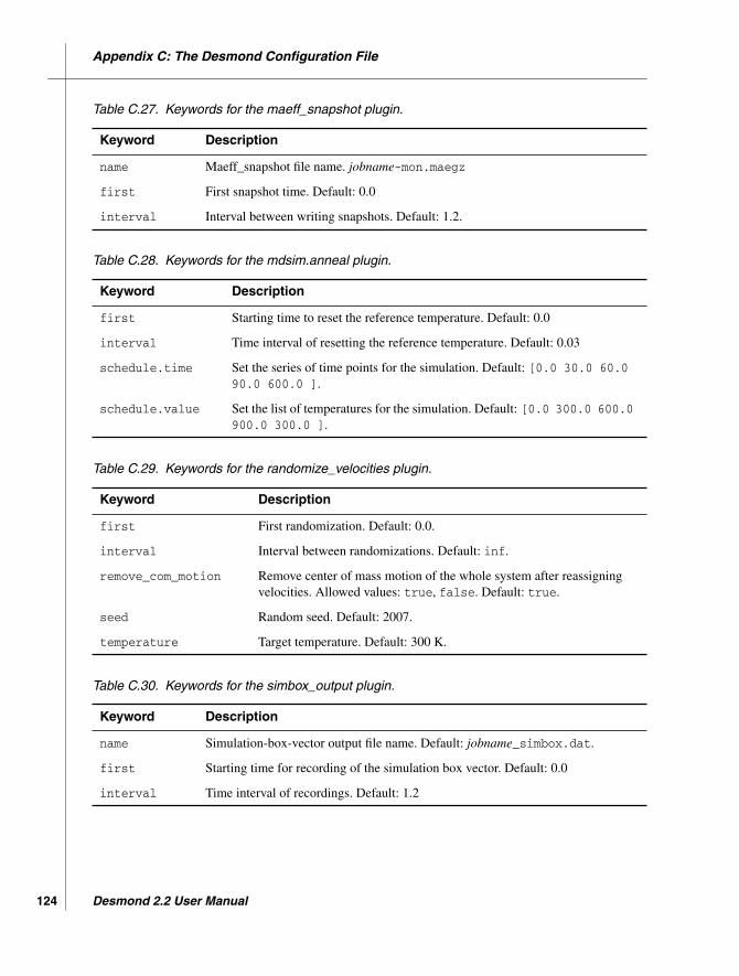
Appendix C: The Desmond Configuration File
124
Table C.27. Keywords for the maeff_snapshot plugin.
Keyword Description
name Maeff_snapshot file name. jobname-mon.maegz
first First snapshot time. Default: 0.0
interval Interval between writing snapshots. Default: 1.2.
Table C.28. Keywords for the mdsim.anneal plugin.
Keyword Description
first Starting time to reset the reference temperature. Default: 0.0
interval Time interval of resetting the reference temperature. Default: 0.03
schedule.time Set the series of time points for the simulation. Default: [0.0 30.0 60.090.0 600.0 ].
schedule.value Set the list of temperatures for the simulation. Default: [0.0 300.0 600.0900.0 300.0 ].
Table C.29. Keywords for the randomize_velocities plugin.
Keyword Description
first First randomization. Default: 0.0.
interval Interval between randomizations. Default: inf.
remove_com_motion Remove center of mass motion of the whole system after reassigningvelocities. Allowed values: true, false. Default: true.
seed Random seed. Default: 2007.
temperature Target temperature. Default: 300 K.
Table C.30. Keywords for the simbox_output plugin.
Keyword Description
name Simulation-box-vector output file name. Default: jobname_simbox.dat.
first Starting time for recording of the simulation box vector. Default: 0.0
interval Time interval of recordings. Default: 1.2
Desmond 2.2 User Manual

Appendix C: The Desmond Configuration File
C.5 Examples
Config files can contain many settings, so constructing them from scratch can be tedious anderror prone. Often it is easier to start with a config file written out from Maestro for a similartype of task. This section provides examples and hints for customizing config files for a fewcommon types of tasks. These examples involve constructing part of the config file and thentaking advantage of a multisim command feature that fills in the missing portions of theconfig file using default values.
C.5.1 FEP Calculations
Below is an example of a config file that contains the complete settings for running an FEPcalculation using multisim with a customized schedule. This file would be provided tomultisim with the -cfg option.
force = {gibbs = {fec_type = "alchemical"i_window = -1lambda = {
bonded = []coulomb = []bondedA = [1.0 1.0 1.0 1.0 1.0 0.857142857143 0.714285714286 0.571428571429
0.428571428571 0.285714285714 0.142857142857 0.0 ]bondedB = [0.0 0.142857142857 0.285714285714 0.428571428571 0.571428571429
Table C.31. Keywords for the status plugin
Keyword Description
first First status report time; written to log file. Example: 0.10
interval Simulation time between reporting status. Example: 1000
Table C.32. Keywords for the trajectory plugin
Keyword Description
first First trajectory output
interval Interval between frames
outdir Directory for trajectory data
write_velocity Include velocities in output. Allowed values: true, false. Default: true.
periodicfix Adjust atoms to make bonds pretty. Allowed values: true, false.Default: true.
Desmond 2.2 User Manual 125

Appendix C: The Desmond Configuration File
126
0.714285714286 0.857142857143 1.0 1.0 1.0 1.0 1.0 ]chargeA = [1.0 0.75 0.5 0.25 0.0 0.0 0.0 0.0 0.0 0.0 0.0 0.0 ]chargeB = [0.0 0.0 0.0 0.0 0.0 0.0 0.0 0.0 0.25 0.5 0.75 1.0 ]vdw = []vdwA = [1.0 1.0 1.0 1.0 1.0 0.674789989504 0.456296209913 0.325045439067
0.24741405481 0.189778434985 0.118514957434 0.0 ]vdwB = [0.0 0.118514957434 0.189778434985 0.24741405481 0.325045439067
0.456296209913 0.674789989504 1.0 1.0 1.0 1.0 1.0 ]}n_windows = 12
}}
gui = {selected_lambda_win = [0 1 2 3 4 5 6 7 8 9 10 11 ]should_autoset_fep = false
}
For multisim FEP jobs:
• Ensure that force.gibbs.i_window is set to -1 (or a negative number), otherwise,multisim runs only 1 window as specified by the value of theforce.gibbs.i_window parameter. By default, this parameter is set to -1.
• Ensure that gui.should_autoset_fep is set to false, otherwise, multisim auto-matically overrides the lambda schedule that you provide. By default, this parameter isset to true.
• If you use a nondefault number of lambda windows, ensure that you setgui.selected_lambda_win to include all windows in the list. For example, if you use7 windows, the gui.selected_lambda_win should be set to [0 1 2 3 4 5 6]. Ifyou miss some windows in the list, simulations will not be run for them. By default thenumber of lambda windows is 12, and gui.selected_lambda_win is set to [0 1 2 34 5 6 7 8 9 10 11].
• Ensure that you set force.gibbs.fec_type to alchemical for relative free energycalculations or ligand_binding for absolute free energy calculations.
Running an FEP job with N windows using an automatically generated schedule is muchsimpler: You can create a config file that has the following contents:
force.gibbs.n_windows = Nforce.gibbs.fec_type = "alchemical"gui.selected_lambda_win = [ 0 1 2 3 ... N-1 ]
and feed multisim’s -cfg option with this .cfg file.
Desmond 2.2 User Manual

Appendix C: The Desmond Configuration File
C.5.2 Replica Exchange
To customize REMD you will need to provide a remd top-level section. In addition you shouldadd the following at the end of the cfg file.
gui.remd.temperature = [300.0 350.0 400.0 450.0 500.0 600.0 700.0800.0]
global_cell.n_replica = 8
C.5.3 Simulated Annealing
You will need to provide a config file for simulated annealing that contains the mdsim.annealand integrator.anneal sections. In addition you should include anneal in the list ofplugins assigned to the mdsim.plugins parameter and set integrator.type to anneal.
C.5.4 Instructing Desmond to Glue Close Solute MoleculesTogether
Periodic boundary conditions can wrap associated solute moleucles separately, such that theyappear on opposite sites of the simulation box. Desmond has a “glue” feature that can signifi-cantly reduce this problem by wrapping associated molecules together.
This feature can be turned on by including the following at the end of the config file:
gui.should_glue = true
Desmond 2.2 User Manual 127

128
Desmond 2.2 User Manual
Desmond User Manual
Appendix D
Appendix D: Analyzing a Simulation from theCommand Line
This appendix documents the command line usage of two related Python scripts and the syntaxof two file formats used for analysis of a simulation. The two Python scripts aresimulation_block_data.py and simulation_block_test.py, and are located in thedirectory $SCHRODINGER/mmshare-vversion/lib/Linux-x86/lib/python2.6/site-packages/schrodinger/application/desmond/. These scripts can be run with the$SCHRODINGER/run command.
D.1 simulation_block_data.py
This command determines simulation properties from the input .log file and block averagesfrom the input .ene file, and writes the results to the output .sba file. The syntax is asfollows:
simulation_block_data.py [-n block-length] [-s simboxfile] -e enefile-l logfile -c sbafile
The options are described in Table D.1.
Table D.1. Options for the simulation_block_data.py command.
Option Description
-e enefile Input .ene file name from a simulation. No default.
-l logfile Input .log file name from a simulation. No default
-c sbafile Output .sba file name. No default.
-n block-length Input block length in ps for calculation of block averages. Default: 10 ps.
-s simboxfile Simbox .dat file name.This is the file that Desmond writes out to track how theshape of the simulation box evolves during the simulation.
Desmond 2.2 User Manual 129

Appendix D: Analyzing a Simulation from the Command Line
130
D.2 simulation_block_test.py
This command evaluates the results in an input.sba file using tests specified in an .sbt file.The output file is a plain text file that prints the job details block from the .sba file and thenprovides information on whether block averages are within the tests specified in the .sbt file.The syntax is as follows:
simulation_block_test.py [-d] -i sbafile -t sbtfile -o outfile
The output file has the following information for each test in the .sbt file.
• Test (Pass or Fail)• Testing criteria from input .sbt file• Corresponding block values from input .sba file
An example output file has the following information besides the job details block from the.sba file.
Test for E: FailTesting criteria: SD = 5.000, Slope = 4.300 kcal/mol/ps , Average = -435320.200+/- 4000.000 kcal/molBlock data: SD = 44.941, Slope = -0.034 kcal/mol/ps, Average = -128666.563 kcal/mol
D.3 Simulation Block Analysis (.sba) File Syntax
The .sba file contains properties obtained from the .log file and block averages from the.ene file. It has a header block followed by the job details block and then by data blocks.
The header block contains the information on the energy and log files and has the followingformat:
Version: versionEnergy_File: enefileLog_File: logfile
The job details block contains the information from the log file about the simulation, such asthe status of the simulation, number of atoms, ensemble, and so on. An example block isshown below:
Block: Job_Details Status = Normal Temperature = 300.0 Job_name = rin Degrees_of_freedom = 103139 Molecules = 3
Desmond 2.2 User Manual

Appendix D: Analyzing a Simulation from the Command Line
Duration = 1.2 Atoms = 50274 Ensemble = MTK_NPTEnd_Block
Subsequent data blocks printed in the .sba file are block averages enclosed between Blockand End_Block lines. A sample data block is shown below:
Block: ETime(ps) E(kcal/mol)5.0 5.010.0 4.9End_Block
The first row is a heading that indicates what quantities are listed below, and it is followed byrows of values. This block indicates that block average for E for data points up to the first 5 pswas 5.0 kcal/mol, and for the next 5 ps (5ps to 10ps) it was 4.9 kcal/mol.
D.4 Simulation Block Test (.sbt) File Syntax
Simulation block test (.sbt) files are used to test the data in .sba files and determine thestability of the simulation. These files contain the test parameters for various properties. Asample test set is as follows:
E {sd = 5.0slope = 4.3average = -435320.2average_tol = 4000.0}
This block indicates that the block values for the property called E in an input .sba file shouldhave following properties:
• Standard deviation < 5.0• Slope (i.e. drift with respect to time) < 4.3• Average should be within -435320.2 4000
Desmond 2.2 User Manual 131

132
Desmond 2.2 User Manual
Desmond User Manual
References
1. Bowers, K.J.; Chow, E.; Xu, H.; Dror, R. O.; Eastwood, M. P.; Gregerson, B. A.;Klepeis, J. L.; Kolossvary, I.; Moraes, M. A.; Sacerdoti, F. D.; Salmon, J. K.; Shan, Y.;Shaw, D. E. Scalable Algorithms for Molecular Dynamics Simulations on CommodityClusters, Proceedings of the ACM/IEEE Conference on Supercomputing(SC06),Tampa, Florida, November 11-17, 2006, http://sc06.supercomputing.org/schedule/event_detail.php?evid=9088.
2. Shaw, D.E. A fast, scalable method for the parallel evaluation of distance-limited pairwise particle interactions. J. Comput. Chem. 2005, 26, 1318.
3. Bowers, K.J.; Dror, R.O.; Shaw, D.E. The midpoint method for parallelization ofparticle simulations. J. Chem. Phys. 2006, 124, 184109.
4. Bowers, K.J.; Dror, R.O.; Shaw, D.E. Zonal methods for the parallel execution of range-limited N-body simulations. J. Comput. Phys. 2007, 221, 303.
5. Lippert, R.A.; Bowers, K.J.; Dror, R. O.; Eastwood, M.P.; Gregersen, B. A.; Klepeis, J.L.; Kolossvary, I.; Shaw, D. E. A common, avoidable source of error in moleculardynamics integrators. J. Chem. Phys. 2007, 126, 046101.
6. Arkin, I.T.; et al. Mechanism of Na+/H+ Antiporting. Science, 2007, 317, 799.
7. Humphrey, W.; Dalke, A.; Schulten, K. VMD - Visual Molecular Dynamics, J. Molec.Graphics, 1996, 14, 33.
8. Cornell, W.D. et al. J. Am. Chem. Soc. 1995, 117, 5179. Parameters converted fromthose at http://amber.scripps.edu/amber9.ffparms.tar.gz
9. Kollman, P. A. Acc. Chem. Res. 1996, 29, 461. Parameters converted from those at http://amber.scripps.edu/amber9.ffparms.tar.gz
10. Wang, J. et al. J. Comp. Chem. 2000, 21, 1049. Parameters converted from those athttp://amber.scripps.edu/amber9.ffparms.tar.gz
11. Hornak et al. Proteins: Structure, Function & Genetics, 2006, 3, 712.
12. Duan, Y. et al. J. Comp. Chem. 2003, 24, 1999. Parameters converted from those athttp://amber.scripps.edu/amber9.ffparms.tar.gz. Bugfix from http://amber.scripps.edu/bugfixes/9.0/bugix.5 applied to correct torsional assignments.
Desmond 2.2 User Manual 133

References
134
13. For proteins: MacKerell, Jr. A. D. et al. J. Phys. Chem. B. 1998, 102, 3586. For ions:Beglov, D. et al. J. Chem. Phys. 1994, 100, 9050. Parameters generated from http://www.pharmacy.umaryland.edu/faculty/amackere/param/toppar/toppar_c31b1.tar.gz.
14. For protein CMAP adjustments: MacKerell, Jr. A. D. et al., J. Comp. Chem. 2004, 25,1400. For proteins: MacKerell, Jr. A. D. et al. J. Phys. Chem. B. 1998, 102, 3586. Forions: Beglov, D. et al. J. Chem. Phys. 1994, 100, 9050. Parameters generated from http://www.pharmacy.umaryland.edu/faculty/amackere/param/toppar/toppar_c31b1.tar.gz.Missing CMAP term applied to protonated HIS.
15. Jorgensen, W. L., et al. J. Am Chem. Soc. 1996, 118, 11225.
16. Damm, W., et al. J. Comput. Chem. 1997, 18, 1955.
17. Jorgensen, W.L., et al. Theochem. 1998, 424, 145.
18. Jorgensen, W.L., et al. J. Phys. Chem. B. 1998, 102, 8049.
19. Rizzo, R.C.; Jorgensen, W.L., J. Am. Chem. Soc. 1999, 121, 4827.
20. Watkins, E.K.; Jorgensen, W.L., J. Phys. Chem. A. 2001, 205, 4118.
21. Kaminski, G. A. et al., J. Phys. Chem. B 2001, 105, 6474.
22. OPLSAA/L reparameterization, version 1 torsions used for SER, version 1 for ASP,version 3 (combined) for LEU, VAL, Jacobson, M.P., et al. J. Phys. Chem. B. 2002, 106,11673. The charges for HISE used in this force field have not been published to ourknowledge.
23. Jacobson, M.P., et al. J. Phys. Chem. B. 2002, 106, 11673.
24. Berendsen, H. J. C. et al. in Intermolecular Forces, edited by B. Pullman (Reidel,Dordrecht,1981), p. 331.
25. Berendsen, H. J. C. et al. J. Phys. Chem. 1987, 91, 6269.
26. Jorgensen, W. L. et al. Mol. Phys. 1983, 79, 926. Parameters as tabulated in: Mahoney,M. W. et al. J. Chem. Phys. 2000, 112, 8910.
27. Neria, E. et al. J. Chem. Phys. 1996, 105, 1902.
28. Jorgensen, W. L. et al. Mol. Phys. 1985, 56, 1381. Parameters as tabulated in: Mahoney,M. W. et al. J. Chem. Phys. 2000, 112, 8910.
29. Horn, H. W. et al. J. Chem. Phys. 2004, 120, 9665
30. Mahoney, M. W. et al. J. Chem. Phys. 2000, 112, 8910.
31. Earl D. J; Deem, M. W.; Phys. Chem. Chem. Phys., 2005, 7, 3910.
Desmond 2.2 User Manual

References
32. Patriksson A; van der Spoel, D. A temperature predictor for parallel tempering simula-tions. Phys. Chem. Chem. Phys. 2008, 10, 2073.
Desmond 2.2 User Manual 135

136
Desmond 2.2 User Manual
Desmond User Manual
Getting Help
Schrödinger software is distributed with documentation in PDF format. If the documentation isnot installed in $SCHRODINGER/docs on a computer that you have access to, you should installit or ask your system administrator to install it.
For help installing and setting up licenses for Schrödinger software and installing documenta-tion, see the Installation Guide. For information on running jobs, see the Job Control Guide.
Maestro has automatic, context-sensitive help (Auto-Help and Balloon Help, or tooltips), andan online help system. To get help, follow the steps below.
• Check the Auto-Help text box, which is located at the foot of the main window. If help isavailable for the task you are performing, it is automatically displayed there. Auto-Helpcontains a single line of information. For more detailed information, use the online help.
• If you want information about a GUI element, such as a button or option, there may beBalloon Help for the item. Pause the cursor over the element. If the Balloon Help doesnot appear, check that Show Balloon Help is selected in the Maestro menu of the mainwindow. If there is Balloon Help for the element, it appears within a few seconds.
• For information about a panel or the tab that is displayed in a panel, click the Help buttonin the panel, or press F1. The help topic is displayed in your browser.
• For other information in the online help, open the default help topic by choosing OnlineHelp from the Help menu on the main menu bar or by pressing CTRL+H. This topic is dis-played in your browser. You can navigate to topics in the navigation bar.
The Help menu also provides access to the manuals (including a full text search), the FAQpages, the New Features pages, and several other topics.
If you do not find the information you need in the Maestro help system, check the followingsources:
• Maestro User Manual, for detailed information on using Maestro• Maestro Command Reference Manual, for information on Maestro commands• Maestro Overview, for an overview of the main features of Maestro• Maestro Tutorial, for a tutorial introduction to basic Maestro features• Desmond Quick Start Guide, for a tutorial introduction to Desmond• Desmond User’s Guide from D. E. Shaw Research, for details of command-line opera-
tion, file formats, and technical background.
Desmond 2.2 User Manual 137

Getting Help
138
• Desmond Frequently Asked Questions pages, athttps://www.schrodinger.com/Desmond_FAQ.html
• Known Issues pages, available on the Support Center.
The manuals are also available in PDF format from the Schrödinger Support Center. Localcopies of the FAQs and Known Issues pages can be viewed by opening the fileSuite_2009_Index.html, which is in the docs directory of the software installation, andfollowing the links to the relevant index pages.
Information on available scripts can be found on the Script Center. Information on availablesoftware updates can be obtained by choosing Check for Updates from the Maestro menu.
If you have questions that are not answered from any of the above sources, contact Schrödingerusing the information below.
E-mail: [email protected]: Schrödinger, 101 SW Main Street, Suite 1300, Portland, OR 97204Phone: (503) 299-1150Fax: (503) 299-4532WWW: http://www.schrodinger.comFTP: ftp://ftp.schrodinger.com
Generally, e-mail correspondence is best because you can send machine output, if necessary.When sending e-mail messages, please include the following information:
• All relevant user input and machine output• Desmond purchaser (company, research institution, or individual)• Primary Desmond user• Computer platform type• Operating system with version number• Desmond version number• Maestro version number• mmshare version number
On UNIX you can obtain the machine and system information listed above by entering thefollowing command at a shell prompt:
$SCHRODINGER/utilities/postmortem
This command generates a file named username-host-schrodinger.tar.gz, which youshould send to [email protected]. If you have a job that failed, enter the followingcommand:
$SCHRODINGER/utilities/postmortem jobid
Desmond 2.2 User Manual

Getting Help
where jobid is the job ID of the failed job, which you can find in the Monitor panel. Thiscommand archives job information as well as the machine and system information, andincludes input and output files (but not structure files). If you have sensitive data in the joblaunch directory, you should move those files to another location first. The archive is namedjobid-archive.tar.gz, and should be sent to [email protected] instead.
If Maestro fails, an error report that contains the relevant information is written to the currentworking directory. The report is named maestro_error.txt, and should be sent [email protected]. A message giving the location of this file is written to the terminalwindow.
More information on the postmortem command can be found in Appendix A of the JobControl Guide
Desmond 2.2 User Manual 139

140
Desmond 2.2 User Manual

120 West 45th Street, 29th Floor
New York, NY 10036
101 SW Main Street, Suite 1300
Portland, OR 97204
8910 University Center Lane, Suite 270
San Diego, CA 92122
Zeppelinstraße 13
81669 München, Germany
Dynamostraße 13
68165 Mannheim, Germany
Quatro House, Frimley Road
Camberley GU16 7ER, United Kingdom
SCHRÖDINGER ®