desktop virtual reality in the enhancement of … · federal university of pernambuco computer...
TRANSCRIPT

FEDERAL UNIVERSITY OF PERNAMBUCO
COMPUTER SCIENCE CENTER
POST-GRADUATION IN COMPUTER SCIENCE
VERONICA TEICHRIEB
�DESKTOP VIRTUAL REALITY IN THE ENHANCEMENT OF
DIGITAL ELEVATION MODELS�
THESIS SUBMITTED TO THE COMPUTER SCIENCE
CENTER OF THE FEDERAL UNIVERSITY OF PERNAMBUCO
IN PARTIAL FULFILLMENT OF THE REQUIREMENTS FOR
THE DEGREE OF DOCTOR IN COMPUTER SCIENCE.
SUPERVISOR: PROF. DR. JUDITH KELNER ([email protected])
CO-SUPERVISOR: PROF. DR. ALEJANDRO C. FRERY ([email protected])
RECIFE - BRAZIL, JANUARY 2004
id32577609 pdfMachine by Broadgun Software - a great PDF writer! - a great PDF creator! - http://www.pdfmachine.com http://www.broadgun.com
ABSTRACT
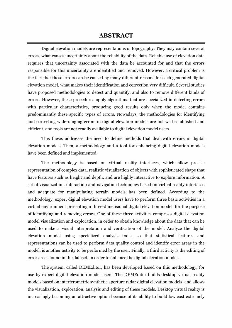
Digital elevation models are representations of topography. They may contain several
errors, what causes uncertainty about the reliability of the data. Reliable use of elevation data
requires that uncertainty associated with the data be accounted for and that the errors
responsible for this uncertainty are identified and removed. However, a critical problem is
the fact that these errors can be caused by many different reasons for each generated digital
elevation model, what makes their identification and correction very difficult. Several studies
have proposed methodologies to detect and quantify, and also to remove different kinds of
errors. However, these procedures apply algorithms that are specialized in detecting errors
with particular characteristics, producing good results only when the model contains
predominantly these specific types of errors. Nowadays, the methodologies for identifying
and correcting wide-ranging errors in digital elevation models are not well established and
efficient, and tools are not readily available to digital elevation model users.
This thesis addresses the need to define methods that deal with errors in digital
elevation models. Then, a methodology and a tool for enhancing digital elevation models
have been defined and implemented.
The methodology is based on virtual reality interfaces, which allow precise
representation of complex data, realistic visualization of objects with sophisticated shape that
have features such as height and depth, and are highly interactive to explore information. A
set of visualization, interaction and navigation techniques based on virtual reality interfaces
and adequate for manipulating terrain models has been defined. According to the
methodology, expert digital elevation model users have to perform three basic activities in a
virtual environment presenting a three-dimensional digital elevation model, for the purpose
of identifying and removing errors. One of these three activities comprises digital elevation
model visualization and exploration, in order to obtain knowledge about the data that can be
used to make a visual interpretation and verification of the model. Analyze the digital
elevation model using specialized analysis tools, so that statistical features and
representations can be used to perform data quality control and identify error areas in the
model, is another activity to be performed by the user. Finally, a third activity is the editing of
error areas found in the dataset, in order to enhance the digital elevation model.
The system, called DEMEditor, has been developed based on this methodology, for
use by expert digital elevation model users. The DEMEditor builds desktop virtual reality
models based on interferometric synthetic aperture radar digital elevation models, and allows
the visualization, exploration, analysis and editing of these models. Desktop virtual reality is
increasingly becoming an attractive option because of its ability to build low cost extremely

ABSTRACT
iii
realistic and interactive environments that can be deployed across every office. The system
improves the processing chain to generate high precision digital elevation models; after the
processing of raw data into a digital elevation model, this model can be analyzed in order to
verify the data correctness and errors can be identified and corrected to enhance it.
The DEMEditor has been used to enhance digital elevation models based on real-
world data, through the realization of case studies. Indeed, the effectiveness of the system has
been confirmed.
Visual interpretation plays an important role in this work, which exploits user�s
knowledge about the data in the decision-making process about (error) areas to be enhanced
in the digital elevation model. The background of the user allows the identification of any
type of error, relieving the need for automatic detection algorithms that specialize in
detecting errors with particular characteristics.
Key words: desktop virtual reality, remote sensing, digital elevation models,
visualization, interaction, editing, error correction.

RESUMO
Modelos digitais de elevação são representações topográficas. Estes modelos podem
conter diversos erros, o que causa incerteza sobre a confiabilidade dos dados. O uso confiável
de dados de elevação requer que a incerteza associada aos dados seja levada em consideração
e que os erros responsáveis por esta incerteza sejam identificados e removidos. Porém, um
problema crítico é o fato de que estes erros podem ser causados por várias razões diferentes
em cada modelo digital de elevação gerado, o que torna a sua identificação e a sua correção
muito difíceis. Vários estudos propuseram metodologias para detectar e quantificar, e
também para remover diferentes tipos de erros. Contudo, estes procedimentos aplicam
algoritmos especializados em detectar erros com características particulares, produzindo
bons resultados apenas quando o modelo contém predominantemente estes tipos específicos
de erros. Atualmente, as metodologias de identificação e de correção de erros de diferentes
tipos em modelos digitais de elevação não estão consolidadas e não são eficientes, e não
existem ferramentas disponíveis para os usuários de modelos digitais de elevação.
Esta tese supre a necessidade de definir métodos para atacar a problemática de erros
em modelos digitais de elevação. Para isso, uma metodologia foi definida e uma ferramenta
foi implementada para melhorar a qualidade de modelos digitais de elevação.
A metodologia é baseada em interfaces de realidade virtual, que permitem a
representação precisa de dados complexos, a visualização realista de objetos com formas
sofisticadas que possuem características como altura e profundidade, e que são bastante
interativas para explorar informações. Um conjunto de técnicas de visualização, interação e
navegação, baseadas em interfaces de realidade virtual e adequadas para manipular modelos
de terreno, foi definido. De acordo com a metodologia, usuários experientes de modelos
digitais de elevação devem realizar três atividades básicas em um ambiente virtual
apresentando um modelo digital de elevação tridimensional, para identificar e remover erros.
Uma destas três atividades é visualizar e explorar o modelo digital de elevação, a fim de obter
conhecimento sobre os dados que pode ser usado para interpretar e verificar visualmente o
modelo. Analisar o modelo digital de elevação usando ferramentas de análise especializadas,
de forma que características e representações estatísticas podem ser usadas para realizar o
controle de qualidade dos dados e identificar áreas de erro no modelo, é outra atividade a ser
realizada pelo usuário. Finalmente, uma terceira atividade é a edição de áreas de erro
encontradas no conjunto de dados, de forma a melhorar o modelo digital de elevação.
O sistema, chamado DEMEditor, foi desenvolvido com base nesta metodologia, para
usuários experientes de modelos digitais de elevação. O DEMEditor constrói modelos de
realidade virtual desktop baseados em modelos digitais de elevação de radar de abertura
RESUMO
v
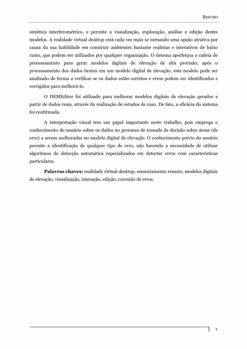
sintética interferométrico, e permite a visualização, exploração, análise e edição destes
modelos. A realidade virtual desktop está cada vez mais se tornando uma opção atrativa por
causa da sua habilidade em construir ambientes bastante realistas e interativos de baixo
custo, que podem ser utilizados por qualquer organização. O sistema aperfeiçoa a cadeia de
processamento para gerar modelos digitais de elevação de alta precisão; após o
processamento dos dados brutos em um modelo digital de elevação, este modelo pode ser
analisado de forma a verificar se os dados estão corretos e erros podem ser identificados e
corrigidos para melhorá-lo.
O DEMEditor foi utilizado para melhorar modelos digitais de elevação gerados a
partir de dados reais, através da realização de estudos de caso. De fato, a eficácia do sistema
foi confirmada.
A interpretação visual tem um papel importante neste trabalho, pois emprega o
conhecimento do usuário sobre os dados no processo de tomada de decisão sobre áreas (de
erro) a serem melhoradas no modelo digital de elevação. O conhecimento prévio do usuário
permite a identificação de qualquer tipo de erro, não havendo a necessidade de utilizar
algoritmos de detecção automática especializados em detectar erros com características
particulares.
Palavras chaves: realidade virtual desktop, sensoriamento remoto, modelos digitais
de elevação, visualização, interação, edição, correção de erros.

ACKNOWLEDGEMENTS
To God, whom the more I learn, the more I appreciate. My gratitude for the many
blessings I have received at his hand.
To my family, thanks you for the support and patience now and in the future. They
helped me �recharge my batteries� when they ran low by always being there when I called.
I wish to thank Cris. More than a single person, he has been a pillar of strength and
support through this long process. His calmness, reflection, and encouragement have enabled
me to see my work through to the end.
Prof. jk, my dear supervisor Dr. Judith Kelner, I wish sincerely to thank the advice
and guidance. I hope I can repay you for your support in some way in the future.
I wish to thank Dr. Alejandro C. Frery, who first opened my eyes to the attractive
world of virtual reality, for the talks and his critical comments.
I wish to thank the Aero-Sensing Team, Andrea Holz, Susanne Och, Frau Dastis,
Tomas Damoiseaux, Andreas Keim, and Oliver Hirsch. I would like to thank them for their
support and friendship, as well as others at this company for their kindest help in daily life. It
was a great experience to work with these enjoyable people. Especially, I would like to thank
João Moreira and Christian Wimmer for invaluable suggestions for the implementation of
the DEMEditor.
I wish to thank also my colleagues in the Networking and Telecommunications
Research Group (GPRT) of the Computer Science Center of the Federal University of
Pernambuco.
To my friends, I always remember and think about you. Forgive me if I don�t keep in
touch as well as I should.
To the members of the committee, thank you for the feedback.
Thanks to CAPES, CNPq, DAAD and Aero-Sensing Radarsysteme GmbH that partially
founded this research.
CONTENTS
LIST OF FIGURES ____________________________________________________________ XII
LIST OF TABLES ______________________________________________________________XV
CHAPTER 1 INTRODUCTION _________________________________________________ 16
1.1 STATEMENT OF THE PROBLEM ________________________________________________ 16
1.2 RESEARCH OBJECTIVES______________________________________________________ 17
1.3 RELEVANCY _______________________________________________________________ 17
1.4 THESIS OUTLINE____________________________________________________________ 18
CHAPTER 2 INTRODUCING REMOTE SENSING ________________________________ 21
2.1 INTRODUCTION TO THE CHAPTER______________________________________________ 21
2.2 CONCEPTS OF REMOTE SENSING ______________________________________________ 21
2.2.1 INTERACTION BETWEEN RADIATION AND TARGET ________________________________ 25
2.2.2 REMOTE SENSING SENSORS __________________________________________________ 30
2.2.2.1 The Radar_______________________________________________________________ 31
2.2.2.2 The Synthetic Aperture Radar _______________________________________________ 36
2.2.2.3 The Interferometric Synthetic Aperture Radar __________________________________ 38
2.2.3 INTERFEROMETRIC SYNTHETIC APERTURE RADAR PROCESSING______________________ 42
2.3 FINAL REMARKS____________________________________________________________ 46
CHAPTER 3 DIGITAL ELEVATION MODELS ___________________________________ 47
3.1 INTRODUCTION TO THE CHAPTER______________________________________________ 47
3.2 CONCEPTS OF DIGITAL ELEVATION MODELS ____________________________________ 47
3.3 CHARACTERIZING A DIGITAL ELEVATION MODEL ________________________________ 48
3.3.1 NON-SPATIAL DIGITAL ELEVATION MODEL CHARACTERIZATION ____________________ 48
3.3.1.1 Moment Statistics_________________________________________________________ 48
3.3.1.2 Accuracy Statistics________________________________________________________ 49
3.3.2 SPATIAL DIGITAL ELEVATION MODEL CHARACTERIZATION _________________________ 50
3.3.2.1 The Variogram___________________________________________________________ 50
3.3.2.2 Spatial Autocorrelation ____________________________________________________ 50
CONTENTS
viii
3.4 ERRORS IN DIGITAL ELEVATION MODELS ______________________________________ 50
3.4.1 GEOMETRIC DISTORTIONS ___________________________________________________ 52
3.4.1.1 Slant Range Scale Distortion ________________________________________________ 52
3.4.1.2 Relief Displacement_______________________________________________________ 53
3.4.1.3 Foreshortening ___________________________________________________________ 53
3.4.1.4 Layover ________________________________________________________________ 54
3.4.1.5 Shadow_________________________________________________________________ 55
3.4.2 IDENTIFYING AND REDUCING ERRORS IN DIGITAL ELEVATION MODELS _______________ 55
3.4.3 QUANTIFYING ERRORS IN DIGITAL ELEVATION MODELS ___________________________ 57
3.4.3.1 Root Mean Squared Error __________________________________________________ 57
3.4.3.2 Error Maps ______________________________________________________________ 58
3.4.3.3 Simulation Methods _______________________________________________________ 58
3.4.3.4 Visualization Techniques___________________________________________________ 58
3.4.3.5 Random Fields ___________________________________________________________ 59
3.5 FINAL REMARKS____________________________________________________________ 60
CHAPTER 4 VISUALIZATION, INTERACTION AND EDITING ____________________ 62
4.1 INTRODUCTION TO THE CHAPTER______________________________________________ 62
4.2 VISUALIZING DIGITAL ELEVATION MODELS _____________________________________ 62
4.2.1 TWO-DIMENSIONAL INTERFACES ______________________________________________ 62
4.2.2 THREE-DIMENSIONAL INTERFACES ____________________________________________ 66
4.3 INTERACTION IN THREE-DIMENSIONAL INTERFACES______________________________ 68
4.4 EDITING METHODS__________________________________________________________ 70
4.4.1 SELECTION METHODS _______________________________________________________ 70
4.4.2 EDITING METHODS _________________________________________________________ 71
4.4.2.1 Cut And Paste Editing of Multiresolution Surfaces_______________________________ 71
4.4.2.2 Point-Based Surface Editing ________________________________________________ 72
4.4.2.3 Image Editing Methods ____________________________________________________ 73
4.5 FINAL REMARKS____________________________________________________________ 74
CHAPTER 5 VIRTUAL REALITY INTERFACES APPLIED TO ENHANCE DIGITAL
ELEVATION MODELS__________________________________________________________ 76
5.1 INTRODUCTION TO THE CHAPTER______________________________________________ 76
5.2 PROBLEM STATEMENT_______________________________________________________ 76
5.3 METHODOLOGY: VIRTUAL REALITY INTERFACES APPLIED TO CORRECT ELEVATION

CONTENTS
ix
ERRORS IN DIGITAL ELEVATION MODELS ___________________________________________ 77
5.3.1 VISUALIZATION OF DIGITAL ELEVATION MODELS_________________________________ 78
5.3.2 INTERACTION IN THE VIRTUAL ENVIRONMENT ___________________________________ 79
5.3.2.1 Two-Dimensional Interaction _______________________________________________ 79
5.3.2.2 Navigation ______________________________________________________________ 79
5.3.2.3 Object Manipulation ______________________________________________________ 80
5.3.2.4 System Control___________________________________________________________ 80
5.3.3 ANALYSIS OF DIGITAL ELEVATION MODELS _____________________________________ 80
5.3.3.1 Histogram_______________________________________________________________ 81
5.3.3.2 Profile__________________________________________________________________ 82
5.3.3.3 Statistical Information _____________________________________________________ 82
5.3.3.4 Position and Height _______________________________________________________ 84
5.3.3.5 Minimum and Maximum Values _____________________________________________ 84
5.3.4 EDITING OF DIGITAL ELEVATION MODELS_______________________________________ 84
5.3.4.1 Selecting Regions Of Interest _______________________________________________ 84
5.3.4.2 Removing Dummy Values__________________________________________________ 84
5.3.4.3 Removing Error Values ____________________________________________________ 85
5.3.4.4 Interpolating Holes________________________________________________________ 85
5.3.4.5 Smoothing ______________________________________________________________ 85
5.3.4.6 Modifying Minimum and Maximum Height Values ______________________________ 89
5.4 SOME CONSIDERATIONS _____________________________________________________ 89
5.5 FINAL REMARKS____________________________________________________________ 90
CHAPTER 6 DEMEDITOR: A VIRTUAL REALITY BASED SYSTEM TO VISUALIZE,
ANALYZE AND EDIT DEMS ____________________________________________________ 91
6.1 INTRODUCTION TO THE CHAPTER______________________________________________ 91
6.2 INTRODUCING THE DEMEDITOR ______________________________________________ 91
6.3 SYSTEM ARCHITECTURE _____________________________________________________ 94
6.3.1 PRESENTATION MODULE ____________________________________________________ 94
6.3.2 REPRESENTATION MODULE __________________________________________________ 97
6.3.2.1 Digital Elevation Model Representation _______________________________________ 97
6.3.2.2 Icons__________________________________________________________________ 101
6.3.2.3 Interaction Components ___________________________________________________ 103
6.3.2.4 Navigation Components___________________________________________________ 106
6.3.3 ANALYSIS MODULE _______________________________________________________ 107
6.3.3.1 Histogram______________________________________________________________ 108
CONTENTS
x
6.3.3.2 Profile_________________________________________________________________ 109
6.3.3.3 Statistical Information ____________________________________________________ 110
6.3.3.4 Position and Height ______________________________________________________ 111
6.3.3.5 Minimum and Maximum Values ____________________________________________ 112
6.3.4 EDITING MODULE _________________________________________________________ 112
6.3.4.1 Selection_______________________________________________________________ 113
6.3.4.2 Interpolation____________________________________________________________ 114
6.3.4.3 Cut ___________________________________________________________________ 115
6.3.4.4 Smooth ________________________________________________________________ 116
6.3.4.5 Definition of Minimum and Maximum Height Values ___________________________ 117
6.4 IMPLEMENTATION ISSUES ___________________________________________________ 118
6.4.1 A HIGH-RESOLUTION VIRTUAL ENVIRONMENT__________________________________ 118
6.4.2 PERFORMANCE ___________________________________________________________ 118
6.4.3 REALISM ________________________________________________________________ 119
6.4.4 INTERACTION IN THE VIRTUAL ENVIRONMENT __________________________________ 119
6.4.4.1 Navigation Strategies _____________________________________________________ 119
6.4.4.2 Object Manipulation _____________________________________________________ 120
6.4.4.3 Interaction Icons_________________________________________________________ 120
6.5 FINAL REMARKS___________________________________________________________ 121
CHAPTER 7 CASE STUDY____________________________________________________ 122
7.1 INTRODUCTION TO THE CHAPTER_____________________________________________ 122
7.2 DATA DESCRIPTION ________________________________________________________ 122
7.3 CASE STUDY ______________________________________________________________ 122
7.3.1 REALISTIC DIGITAL ELEVATION MODEL VISUALIZATION __________________________ 123
7.3.2 USER X DIGITAL ELEVATION MODEL: INTUITIVE AND EFFECTIVE INTERACTION ________ 124
7.3.3 DIGITAL ELEVATION MODEL EXPLORATION THROUGH NAVIGATION _________________ 124
7.3.4 2D EDITING METHODS APPLIED IN A 3D ENVIRONMENT___________________________ 125
7.4 THE DEMEDITOR SYSTEM: EFFECTIVE OR NOT? _______________________________ 126
7.5 FINAL REMARKS___________________________________________________________ 128
CHAPTER 8 CONCLUSION___________________________________________________ 129
8.1 CONTRIBUTIONS ___________________________________________________________ 129
8.1.1 A METHODOLOGY TO ENHANCE DIGITAL ELEVATION MODELS _____________________ 129
8.1.2 THE DEMEDITOR SYSTEM __________________________________________________ 130

CONTENTS
xi
8.1.3 THREE-DIMENSIONAL INTERFACES ___________________________________________ 131
8.2 FUTURE WORKS ___________________________________________________________ 131
8.2.1 IMMERSIVE VIRTUAL REALITY INTERFACES ____________________________________ 131
8.2.2 EVALUATION OF INTERFACES AND INTERACTION TECHNIQUES______________________ 132
8.2.3 AUTOMATIC ERROR IDENTIFICATION __________________________________________ 132
8.2.4 REPRESENTATION OF DIGITAL ELEVATION MODEL ERRORS ________________________ 132
8.2.5 QUANTIFICATION OF DIGITAL ELEVATION MODEL ERRORS ________________________ 132
8.2.6 EDITING METHODS ________________________________________________________ 132
8.2.7 COLLABORATIVE EDITING OF DIGITAL ELEVATION MODELS _______________________ 133
8.2.8 SCENE MODELING IN THE DEMEDITOR ________________________________________ 133
8.2.9 OTHER APPLICATION AREAS ________________________________________________ 133
8.3 CLOSING THOUGHTS _______________________________________________________ 134
REFERENCES ________________________________________________________________ 135
BIBLIOGRAPHY_________________________________________________________________ 135
ADDITIONAL REFERENCES _______________________________________________________ 140
APPENDIX CLASS DIAGRAM __________________________________________________ 145

LIST OF FIGURES
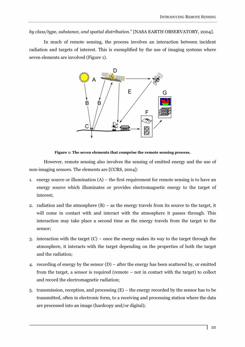
FIGURE 1: THE SEVEN ELEMENTS THAT COMPRISE THE REMOTE SENSING PROCESS. _____________ 22
FIGURE 2: WAVELENGTHS. _________________________________________________________ 23
FIGURE 3: THE ELECTROMAGNETIC SPECTRUM. _________________________________________ 24
FIGURE 4: THE MICROWAVE REGION. _________________________________________________ 24
FIGURE 5: ENERGY INTERACTING WITH THE ATMOSPHERE: A) SCATTERING; B) ABSORPTION. _____ 25
FIGURE 6: FORMS OF INTERACTION BETWEEN RADIATION AND TARGET.______________________ 26
FIGURE 7: SURFACE REFLECTION: A) SPECULAR REFLECTION; B) DIFFUSE REFLECTION. _________ 26
FIGURE 8: LOOK DIRECTION OF THE SENSOR: A) WEST-EAST DIRECTION; B) EAST-WEST DIRECTION. 28
FIGURE 9: A TYPICAL SENSOR SYSTEM. _______________________________________________ 29
FIGURE 10: REMOTE SENSING SENSORS: A) PASSIVE SENSOR; B) ACTIVE SENSOR. ______________ 30
FIGURE 11: SCENES IMAGED WITH DIFFERENT WAVELENGTHS: A) X-BAND; B) P-BAND. _________ 32
FIGURE 12: IMAGING GEOMETRY OF A RADAR SYSTEM.___________________________________ 34
FIGURE 13: RESOLUTION: A) RANGE RESOLUTION; B) AZIMUTH RESOLUTION. _________________ 35
FIGURE 14: THE SAR METHOD. _____________________________________________________ 36
FIGURE 15: IMAGING GEOMETRY OF A SAR SYSTEM. ____________________________________ 37
FIGURE 16: REFLECTIVITY OF A RESOLUTION CELL.______________________________________ 37
FIGURE 17: IMAGING PRINCIPLE OF A SAR SYSTEM. _____________________________________ 38
FIGURE 18: IMAGING PRINCIPLE OF AN INSAR SYSTEM. __________________________________ 39
FIGURE 19: PHASE DIFFERENCE OF TWO ELECTROMAGNETIC WAVES.________________________ 39
FIGURE 20: AN INTERFEROGRAM.____________________________________________________ 40
FIGURE 21: COHERENCE OF AN IMAGED SURFACE: A) COHERENCE SCENE; B) X-BAND SAR SCENE. 41
FIGURE 22: 2D AND 3D VIEWS OF THE TERRAIN HEIGHT.__________________________________ 41
FIGURE 23: MEASURE PRINCIPLE OF AN INSAR SYSTEM. _________________________________ 42
FIGURE 24: INSAR PROCESSING CHAIN. _______________________________________________ 43
FIGURE 25: RESULTS PRODUCED BY DIFFERENT STEPS OF AN INSAR PROCESSING CHAIN.________ 45
FIGURE 26: SLANT RANGE SCALE DISTORTION. _________________________________________ 52
FIGURE 27: SLANT RANGE SCALE DISTORTION: A) SLANT RANGE IMAGE; B) GROUND RANGE IMAGE. 53
FIGURE 28: FORESHORTENING. ______________________________________________________ 53
FIGURE 29: RADAR IMAGE WITH FORESHORTENING EFFECTS. ______________________________ 54
FIGURE 30: LAYOVER._____________________________________________________________ 54
FIGURE 31: RADAR IMAGE WITH LAYOVER EFFECTS. _____________________________________ 55
FIGURE 32: RADAR IMAGE WITH SHADOW EFFECTS. _____________________________________ 55
TABLE 1: SYNTHESIS OF ERROR IDENTIFICATION, QUANTIFICATION AND REMOVAL METHODS. ____ 61
FIGURE 33: AN EXAMPLE OF DEM PRESENTED AS CONTOUR LEVELS. _______________________ 63
FIGURE 34: CONTOUR LEVELS OF A DEM. _____________________________________________ 64

LIST OF FIGURES
xiii
FIGURE 35: GRAY LEVEL VISUALIZATION OF A DEM. ____________________________________ 64
FIGURE 36: PERSPECTIVE VISUALIZATION OF A DEM. ____________________________________ 65
FIGURE 37: COMPOUND VISUALIZATION OF A DEM. _____________________________________ 66
FIGURE 38: 3D SURFACE MODEL GENERATED FROM DEM DATA. ___________________________ 67
FIGURE 39: SURFACE VISUALIZATION USING THE KINETIC VISUALIZATION TECHNIQUE. _________ 68
FIGURE 40: BOUNDARY DEFINITION WITH INTELLIGENT SCISSORS. _________________________ 71
FIGURE 41: SELECTION: A) IMAGE OF A BIRD; B) REGION DEFINITION WITH INTELLIGENT PAINT. __ 71
FIGURE 42: CUT AND PASTE ALGORITHM FOR EDITING OF MULTIRESOLUTION SURFACES. ________ 72
FIGURE 43: EDITING OF A POINT-SAMPLED OBJECT: CARVING. _____________________________ 72
FIGURE 44: OBJECT-BASED IMAGE BENDING. ___________________________________________ 74
FIGURE 45: CONTRAST ENHANCEMENT USING THE LINEAR STRETCH METHOD. ________________ 82
FIGURE 46: THE MEAN FILTER: A) ORIGINAL IMAGE; B) IMAGE SMOOTHED WITH A MEAN FILTER. _ 86
FIGURE 47: ILLUSTRATING THE FUNCTIONING OF A MEDIAN FILTER._________________________ 87
FIGURE 48: MEDIAN FILTER: A) ORIGINAL IMAGE; B) SALT AND PEPPER NOISE; C) SMOOTHED.____ 88
FIGURE 49: A GRAPHICS OBJECT TREE.________________________________________________ 93
FIGURE 50: THE ARCHITECTURE OF THE DEMEDITOR. ___________________________________ 94
FIGURE 51: THE PRESENTATION MODULE. _____________________________________________ 95
FIGURE 52: THE 2D INTERFACE OF THE DEMEDITOR. ____________________________________ 96
FIGURE 53: THE 3D INTERFACE OF THE DEMEDITOR. ____________________________________ 97
FIGURE 54: THE REPRESENTATION MODULE. ___________________________________________ 97
FIGURE 55: THE DEM SURFACE RENDERED AS A WIRE MESH OBJECT. _______________________ 98
FIGURE 56: ZOOMED 3D SURFACE.___________________________________________________ 99
FIGURE 57: COMPOUND VISUALIZATION OF A DEM IN THE VIRTUAL ENVIRONMENT. __________ 100
FIGURE 58: THE DEM WRAPPED WITH ITS AMPLITUDE PICTURE. __________________________ 101
FIGURE 59: ZOOMING THE SURFACE USING A ZOOM BOX ICON. ____________________________ 102
FIGURE 60: INTERACTION MENUS: A) MAIN MENU; B) DISPLAY WINDOW; C) ZOOM WINDOW. ____ 104
FIGURE 61: INTERACTING WITH THE DEM THROUGH THE ZOOM TOOL. _____________________ 104
FIGURE 62: INTERACTING WITH THE 3D ENVIRONMENT: A) OPTIONS MENU; B) EDITING MENU. __ 105
FIGURE 63: SPOTLIGHT: A) UNSELECTED; B) SELECTED/TRANSLATION; C) ROTATION; D) SCALE. _ 106
FIGURE 64: THE NAVIGATION TOOLBAR. _____________________________________________ 106
FIGURE 65: THE ANALYSIS MODULE. ________________________________________________ 108
FIGURE 66: THE ZOOM WINDOW AND ITS CORRESPONDING HISTOGRAM. ____________________ 108
FIGURE 67: SELECTING THE WINDOW WHERE THE PROFILE LINE WILL BE DRAWN. _____________ 109
FIGURE 68: PROFILE: A) DRAWING THE LINE; B) VIEWING GRAPHICALLY THE HEIGHT VARIATIONS. 110
FIGURE 69: OBTAINING STATISTICAL INFORMATION ABOUT A DATASET. ____________________ 111
FIGURE 70: THE POSITION AND HEIGHT VISUALIZATION WINDOW. _________________________ 112
FIGURE 71: THE EDITING MODULE. __________________________________________________ 112

LIST OF FIGURES
xiv
FIGURE 72: SELECTING A ROI IN THE VIRTUAL ENVIRONMENT. ___________________________ 113
FIGURE 73: INTERPOLATING THE DATA CONTAINED IN A ROI. ____________________________ 115
FIGURE 74: CUTTING OUT THE ROI. _________________________________________________ 116
FIGURE 75: THE VIRTUAL DEM SMOOTHED WITH A MEAN FILTER. _________________________ 117
FIGURE 76: MODIFYING THE MINIMUM HEIGHT VALUE OF THE DEM: A) BEFORE; B) AFTER._____ 118
FIGURE 77: VISUALIZING A DEM: A) 2D GRAYSCALE IMAGE; B) 3D SURFACE OBJECT._________ 123
FIGURE 78: ENHANCING REALISM AND COMPREHENSION: A) COLORS; B) COMPOUND VIEW._____ 123
FIGURE 79: INTERACTIVE EDITING: A) ORIGINAL DEM; B) DEM WITH LOWER MAXIMUM VALUE. 124
FIGURE 80: REMOVING DUMMY VALUES: A) ORIGINAL DEM; B) DEM WITHOUT HOLES. _______ 125
FIGURE 81: CUTTING OUT ERROR AREAS: A) A ROI IS DEFINED; B) THE DATA ARE CUT OUT._____ 126
FIGURE 82: INTERPOLATING AND SMOOTHING: A) ORIGINAL DEM; B) EDITED DEM. __________ 126

LIST OF TABLES
TABLE 1: SYNTHESIS OF ERROR IDENTIFICATION, QUANTIFICATION AND REMOVAL METHODS. ____ 61

CHAPTER 1
INTRODUCTION
The subject of this thesis is enhancing digital elevation models (DEMs) through its
editing and the correction of errors in these models using non-immersive virtual reality (VR).
The deployment of desktop VR is increasingly becoming and attractive option for developing
applications that need realistic and interactive three-dimensional (3D) presentation of data
because of its ability to build low cost realistic and interactive environments that can be
utilized across every office. The correction of errors in DEMs has been discussed for some
years now, but still there are no technical solutions good enough for convincing remote
sensing companies to implement them and/or pay for them and commercial solutions
available. Error identification and correction methods need to address different types of
error, originated by diverse causes. The big challenge is to develop methodologies and tools
to enhance DEMs in an intuitive and efficient way, usable by expert DEM users, in order to
produce high quality DEMs.
In the following sections, the problem this thesis aims to resolve and the objectives
that will be followed proposing a solution are presented. Following on from this, the
relevancy of this work is justified by describing its contributions to the remote sensing and
virtual reality communities, as it is an interdisciplinary work. Finally, the structure of this
document is presented.
1.1 STATEMENT OF THE PROBLEM
DEMs are models of the elevation surface and are used in many types of geographic
analyses. DEMs are used for map visualization, hydrologic modeling, terrain modeling,
business applications and land use planning. Products derived from DEMs include but are
not limited to elevation contours, shaded relief, watershed boundaries, and ridge detection.
As models of topography, DEMs have inherent limitations and contain
errors [CONCAR, 2004; USGS, 1997]. Error is defined as the departure of a measurement
from its true value. The exact nature and location of errors in spatial datasets, specifically
elevation data, cannot be precisely determined in general. The lack of knowledge about this
error in spatial data results in uncertainty, which is a measure of what is not known.
Results of an informal survey conducted during this thesis through the contact with
experienced DEM users suggest that the methods used by the community to identify,
quantify and remove errors in DEMs are assorted. There do not appear to be consolidated
methodologies that are applied to DEM data to address problems of correcting errors.
INTRODUCTION
17
Decisions about how to manage errors in the data are made by individual DEM users.
Nevertheless, the survey suggests that DEM users appear to be trying out various methods to
identify, quantify and remove errors from DEMs, based on two-dimensional (2D) tools.
According to the feedback of this contact with DEM users, a system providing realistic
visualization methods and interactive exploration tools, well-known analysis functions and
editing tools to correct errors in DEMs is needed by the community.
This thesis addresses the need to develop methodologies that deal with errors in
DEMs. A methodology and a tool for correcting errors in DEMs will be defined and
implemented.
1.2 RESEARCH OBJECTIVES
The objectives of this research are:
to develop a methodology to correct elevation errors in DEMs, based on the use of 3D
interfaces to visualize, explore, analyze and edit terrain models;
to develop a system, called DEMEditor, that implements the proposed methodology;
to validate the implemented methodology, using the DEMEditor with DEMs based on
real-world data.
1.3 RELEVANCY
Errors are a fact in spatial data. Reliable and valid use of elevation data requires that
uncertainty associated with the data be accounted for and that the errors responsible for this
uncertainty are identified and removed. However, a critical problem is the fact that these
errors can be caused by many different reasons for each generated DEM, what makes their
identification and correction very difficult. Methods for correcting wide-ranging errors in
DEMs through a simple and efficient procedure are not readily available to DEM users.
This research provides users with an easily accessible method to reduce errors in
elevation models through the use of 3D interfaces for visualization, exploration, analysis and
editing. The methodology developed and utilized in this research can be applied to other
editing procedures, in addition to the correction of errors performed in this research. Results
of this research can benefit producers of DEMs as well as end-users, which will become more
accurate elevation models.
The applicability of non-immersive VR interfaces to the remote sensing field of
application is also highlighted, not only to perform visualization, but also to approach the real
problem of correcting elevation errors in DEMs. This research intends to offer to the remote
sensing community a professional tool developed for experienced DEM users to visualize and

INTRODUCTION
18
explore large terrain models, analyze the data using well-established analysis functions, and
edit elevation models in order to remove their errors.
This thesis differs from previous related investigations in the following ways:
no previous investigations have provided a systematic method for addressing the problem
of identifying and correcting wide-ranging errors in DEMs through an intuitive and
efficient procedure, based on the knowledge of experienced users and applying 3D
interfaces;
no other studies have implemented a complete tool to identify and remove errors in
DEMs that is accessible to many DEM users. Prior to this undertaking there were no tools
to simultaneously visualize and explore DEMs, analyze the data in order to verify its
accuracy, and edit errors in the elevation data, both, in two and three dimensions;
desktop VR interfaces have largely been applied for visualization of terrain data, but have
not been used to develop a complete tool for the remote sensing community, composed
not only of visualization and interaction components, peculiar to this kind of interface,
but also of specialized analysis functions and sophisticated editing methods;
several analysis and editing tools have been implemented in the system developed by this
thesis, based on requirements of expert DEM users. These tools have been re-
implemented based on sophisticated commercial tools and adapted to fulfill these
requirements, or specified and developed from scratch.
1.4 THESIS OUTLINE
This thesis is structured for introducing the concepts related to remote sensing and
VR and describing the proposal in a logical fashion. In this chapter, the problem of correcting
errors in DEMs was introduced and the objectives of the thesis were outlined. The remainder
of this document is organized as follows.
Chapter two, Introducing Remote Sensing, introduces the main concepts of remote
sensing, which represents the application area of this thesis. Doing remote sensing involves
some steps, which require the use of sophisticated devices and complex algorithms. The
process of collecting data about a specific terrain area, in order to be successful, needs a
precise configuration and control of the platform that holds the imaging sensor, and of the
sensor itself. After the imaging process, the collected raw data have to be processed so that
products such as orthorectified synthetic aperture radar (SAR) images and DEMs can be
produced. The algorithms that compose the processing chain are based on complex methods
(e.g., demultiplexing, motion compensation). Another important topic in the remote sensing
process is the interaction between electromagnetic radiation and the target to be imaged.

INTRODUCTION
19
This subject has to be understood very well, so that precise data may be produced.
Being DEMs and their inherent elevation errors the object of study of this research, a
special attention will be given to the features and problems related to them. Some
characterization methods can be used to obtain knowledge about the data, and analyses can
be performed regarding its precision. Elevation models contain height errors due to the
process used to collect the raw data, the methods applied to process the raw data into a DEM,
and also the nature of the imaged relief. Before an elevation model can be released as a
reliable product, it passes through quality controls, and therefore error identification,
quantification and reduction methods need to be used in order to provide a product of
quality. Some of the most important related works, actually done about these subjects, will be
presented by this thesis in the third chapter, Digital Elevation Models.
VR interfaces (immersive or not) have proven to be very efficient to visualize and
explore large amounts of data. They also offer very realistic and intuitive presentations of
objects with features such as depth, height and complex shapes. Due to this fact 3D interfaces
(non-immersive) will be studied and applied by this research, to facilitate the processes of
information exploration and analysis. Their main advantages over traditional 2D interfaces,
which are high interaction and realistic visualization, will be described in the chapter
Visualization, Interaction and Editing. Editing methods will also be described in this chapter,
once this thesis proposes the correction of elevation errors through the use of editing tools. In
the literature, research works focus on editing methods based on pixels, surface points
(surfels), regions of interest (ROIs), contour levels, images, image objects and surfaces.
Editing operations to be used in different levels are also approached: clone, brush, cut, paste,
move, scale, rotate, stretch, bend, warp, delete, smooth, and fill holes. In order to edit, the
area of interest has to be selected; studies related to the selection in the pixel, object and
surface level will also be presented.
The fifth chapter, Virtual Reality Interfaces Applied to Enhance Digital Elevation
Models, describes the methodology developed for this thesis. The approach is based on VR
interfaces, which are used to perform visualization and exploration of the data, as well as
statistical analyses in order to identify errors, and to edit errors, found in the models.
Chapter six, DEMEditor: a Virtual Reality Based System to Visualize, Analyze and
Edit DEM, presents the DEMEditor, a system that implements the visualization and
interaction techniques, analysis functions and editing methods that compose the
methodology described in the previous chapter.
In chapter seven, Case Study, real-world datasets are enhanced applying the
DEMEditor. The effectiveness of the system is verified.

INTRODUCTION
20
Finally, the chapter Conclusion highlights the contributions of this thesis and
proposes future applications for the methods and ideas developed herein.
CHAPTER 2
INTRODUCING REMOTE SENSING
2.1 INTRODUCTION TO THE CHAPTER
This chapter intends to highlight the application domain of this thesis: remote
sensing. Its main concepts are introduced, beginning with the definition of the term �remote
sensing�.
Doing remote sensing involves basically seven elements: (1) the energy source, (2) the
relation between radiation and atmosphere, (3) the interaction of the radiation with the
target, (4) the sensor used to perform remote sensing, (5) the transmission, reception and
processing of data collected by the sensor, (6) the interpretation and analysis of the processed
data, and (7) the application of this information.
Each of these elements is briefly described in this chapter, giving emphasis to the
interaction process of electromagnetic waves with the target being sensed, and the use of
interferometric SAR microwave sensors. This emphasis is given firstly because the
methodology proposed by this thesis, as well as the software developed to apply and validate
this methodology are based on DEMs generated from raw data collected by such sensors. It is
also important to understand the results produced by different wavelengths and scene
features interacting together, in order to facilitate the interpretation of the data and to
comprehend why they present errors.
2.2 CONCEPTS OF REMOTE SENSING
Remote sensing is the process of gathering information about something without
touching it. Imagine the following scenario: a day at the beach, seeing the glitter of the ocean
and the people in their brightly colored swimsuits, and hearing the roar of the waves and
feeling the warmth of the sun. This is doing remote sensing.
The history of remote sensing is bonded to the military use of the technology to do
Earth observation. But, recalling that remote sensing is simply obtaining information about
an object without coming into direct contact with it, it can be said that it is a process that has
been around a long time [NASA OBSERVATORIUM - History, 2004; COVRE, 1997].
The term �remote sensing� is usually used to describe � the science of identifying,
observing, and measuring an object without coming into direct contact with it. This process
involves the detection and measurement of radiation of different wavelengths reflected or
emitted from distant objects or materials, by which they may be identified and categorized
INTRODUCING REMOTE SENSING
22
by class/type, substance, and spatial distribution.� [NASA EARTH OBSERVATORY, 2004].
In much of remote sensing, the process involves an interaction between incident
radiation and targets of interest. This is exemplified by the use of imaging systems where
seven elements are involved (Figure 1).
Figure 1: The seven elements that comprise the remote sensing process.
However, remote sensing also involves the sensing of emitted energy and the use of
non-imaging sensors. The elements are [CCRS, 2004]:
1. energy source or illumination (A) � the first requirement for remote sensing is to have an
energy source which illuminates or provides electromagnetic energy to the target of
interest;
2. radiation and the atmosphere (B) � as the energy travels from its source to the target, it
will come in contact with and interact with the atmosphere it passes through. This
interaction may take place a second time as the energy travels from the target to the
sensor;
3. interaction with the target (C) � once the energy makes its way to the target through the
atmosphere, it interacts with the target depending on the properties of both the target
and the radiation;
4. recording of energy by the sensor (D) � after the energy has been scattered by, or emitted
from the target, a sensor is required (remote � not in contact with the target) to collect
and record the electromagnetic radiation;
5. transmission, reception, and processing (E) � the energy recorded by the sensor has to be
transmitted, often in electronic form, to a receiving and processing station where the data
are processed into an image (hardcopy and/or digital);

INTRODUCING REMOTE SENSING
23
6. interpretation and analysis (F) � the processed image is interpreted, visually and/or
digitally, to extract information about the target which was illuminated;
7. application (G) � the final element of the remote sensing process is achieved when
applying the information extracted from the imagery about the target in order to better
understand it, reveal some new information, or assist in solving a particular problem.
The first requirement for remote sensing is to have an energy source to illuminate the
target (unless the sensed energy is being emitted by the target). This energy is in the form of
electromagnetic radiation (element A in Figure 1). A wave or electromagnetic radiation is
described, among others, by its length and frequency, which are particularly important
concepts for understanding remote sensing [NASA SIM, 2004].
The wavelength is the length of one wave cycle, which can be measured as the distance
between two crests (hills) or two troughs (valleys) of a wave (Figure 2). Wavelength is usually
represented by the Greek letter lambda ( ë ), and is measured in meters (m) or some factor of
meters such as nanometers (nm, 910
meters), micrometers (m, 610
meters) or
centimeters (cm, 210
meters). The frequency refers to the number of cycles of a wave
passing a fixed point per unit of time. Frequency is normally measured in hertz (Hz),
equivalent to one cycle per second, and various multiples of hertz. The shorter the
wavelength, the higher the frequency, and the longer the wavelength, the lower the
frequency.
Figure 2: Wavelengths.
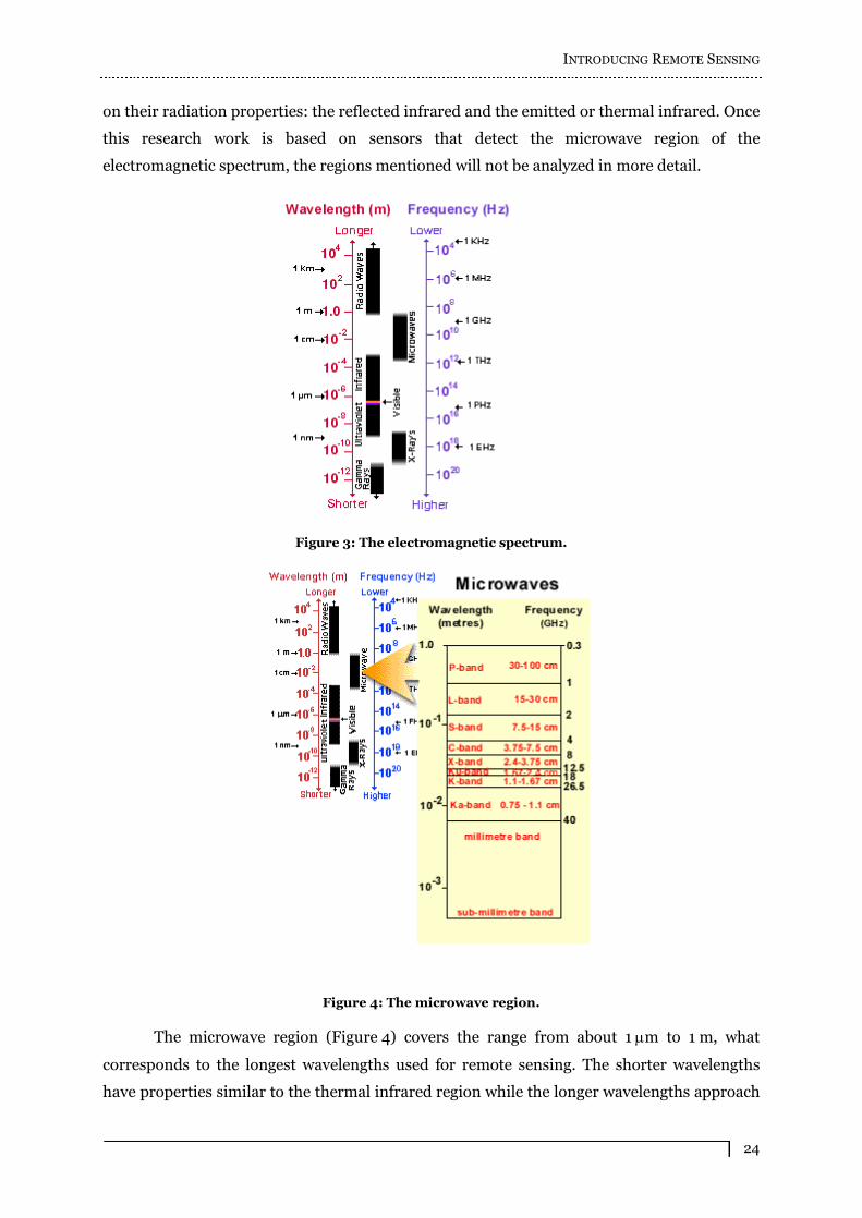
The electromagnetic spectrum (Figure 3) ranges from the shorter wavelengths
(including gamma and x-rays) to the longer wavelengths (including microwaves and
broadcast radio waves). There are several regions of the electromagnetic spectrum that are
useful for remote sensing. For most purposes, the ultraviolet portion of the spectrum has the
shortest wavelengths that are practical for remote sensing. The light that our eyes can detect
is part of the visible spectrum. The infrared region can be divided into two categories based
INTRODUCING REMOTE SENSING
24
on their radiation properties: the reflected infrared and the emitted or thermal infrared. Once
this research work is based on sensors that detect the microwave region of the
electromagnetic spectrum, the regions mentioned will not be analyzed in more detail.
Figure 3: The electromagnetic spectrum.
Figure 4: The microwave region.
The microwave region (Figure 4) covers the range from about 1 m to 1 m, what
corresponds to the longest wavelengths used for remote sensing. The shorter wavelengths
have properties similar to the thermal infrared region while the longer wavelengths approach

INTRODUCING REMOTE SENSING
25
the wavelengths used for radio broadcasts.
Before radiation used for remote sensing reaches the Earth�s surface it has to travel
through some distance on the Earth�s atmosphere (element B in Figure 1). Particles and gases
in the atmosphere can affect the incoming light and radiation causing scattering and
absorption.
Scattering (Figure 5a) occurs when the particles or large gas molecules present in the
atmosphere interact with the electromagnetic radiation and redirected it from the original
path. The quantity of scattering that takes place depends on several factors including the
wavelength of the radiation, the abundance of particles or gases, and the distance the
radiation travels through the atmosphere.
a
b
Figure 5: Energy interacting with the atmosphere: a) scattering; b) absorption.
Absorption (Figure 5b) is the other main mechanism at work when electromagnetic
radiation interacts with the atmosphere. In contrast to scattering, this phenomenon causes
molecules in the atmosphere to absorb energy at various wavelengths. Ozone, carbon dioxide,
and water vapor are the three main atmospheric constituents that absorb radiation.
In order to perform remote sensing, it must be chosen the areas of the spectrum that
are not severely affected by atmospheric absorption. These areas are called atmospheric
windows.
2.2.1 INTERACTION BETWEEN RADIATION AND TARGET
Radiation that is not absorbed or scattered in the atmosphere can reach and interact
with the Earth�s surface (element C in Figure 1). There are three forms of interaction
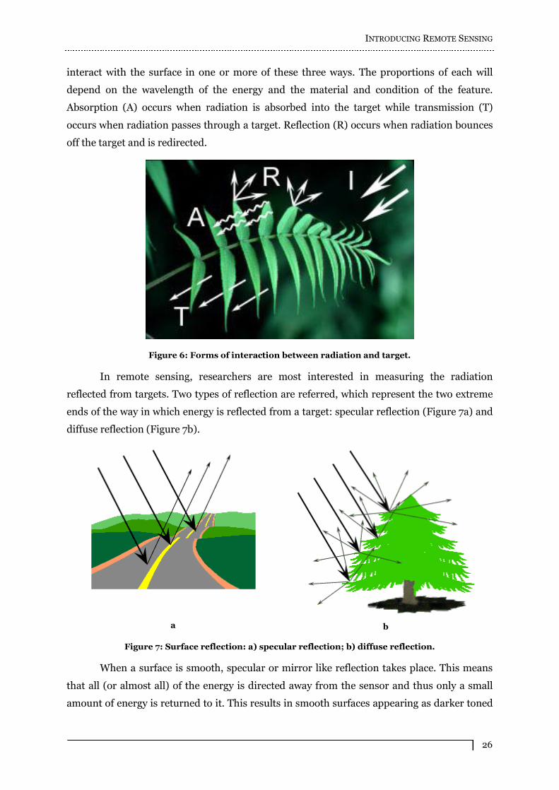
(Figure 6) that can take place when energy strikes, or is incident (I) upon the surface. These
are: absorption (A), transmission (T), and reflection (R). The total incident energy will
INTRODUCING REMOTE SENSING
26
interact with the surface in one or more of these three ways. The proportions of each will
depend on the wavelength of the energy and the material and condition of the feature.
Absorption (A) occurs when radiation is absorbed into the target while transmission (T)
occurs when radiation passes through a target. Reflection (R) occurs when radiation bounces
off the target and is redirected.
Figure 6: Forms of interaction between radiation and target.
In remote sensing, researchers are most interested in measuring the radiation
reflected from targets. Two types of reflection are referred, which represent the two extreme
ends of the way in which energy is reflected from a target: specular reflection (Figure 7a) and
diffuse reflection (Figure 7b).
a
b
Figure 7: Surface reflection: a) specular reflection; b) diffuse reflection.
When a surface is smooth, specular or mirror like reflection takes place. This means
that all (or almost all) of the energy is directed away from the sensor and thus only a small
amount of energy is returned to it. This results in smooth surfaces appearing as darker toned

INTRODUCING REMOTE SENSING
27
areas on an image. Diffuse reflection occurs when the surface is rough and the energy is
reflected almost uniformly in all directions, so that a significant portion of the energy will be
backscattered to the sensor. Thus, rough surfaces will appear lighter in tone on an
image [FREEMAN, 2004]. Most Earth surface features lie somewhere between perfectly
specular or perfectly diffuse reflectors. A particular target reflects specularly or diffusely, or
somewhere in between, depending on the surface roughness of the feature in comparison to
the wavelength of the incoming radiation. If the wavelengths are much smaller than the
surface variations or the particle sizes that make up the surface, diffuse reflection will
dominate. For example, fine-grained sand would appear fairly smooth to long wavelength
microwaves but would appear quite rough to the visible wavelengths.
The relationship between viewing geometry and the geometry of the surface features
plays an important role in how the sensor energy interacts with targets and their
corresponding brightness on an image. The local incidence angle (see Figure 12 in section
The Radar) is the angle between the sensor beam and a line perpendicular to the slope at the
point of incidence. Thus, the local incidence angle takes into account the local slope of the
terrain in relation to the sensor beam. With flat terrain, the local incidence angle is the same
as the look angle (Figure 12b) of the sensor, and with terrain with another type of relief, these
angles are different. Generally, slopes facing towards the sensor will have small local
incidence angles, causing relatively strong backscattering to the sensor, which results in a
bright toned appearance in an image.
Variations in viewing geometry will accentuate and enhance topography and relief in
different ways, such that varying degrees of foreshortening, layover, and shadow may occur
depending on surface slope, orientation, and shape. These effects are described in detail in
section Geometric Distortions.
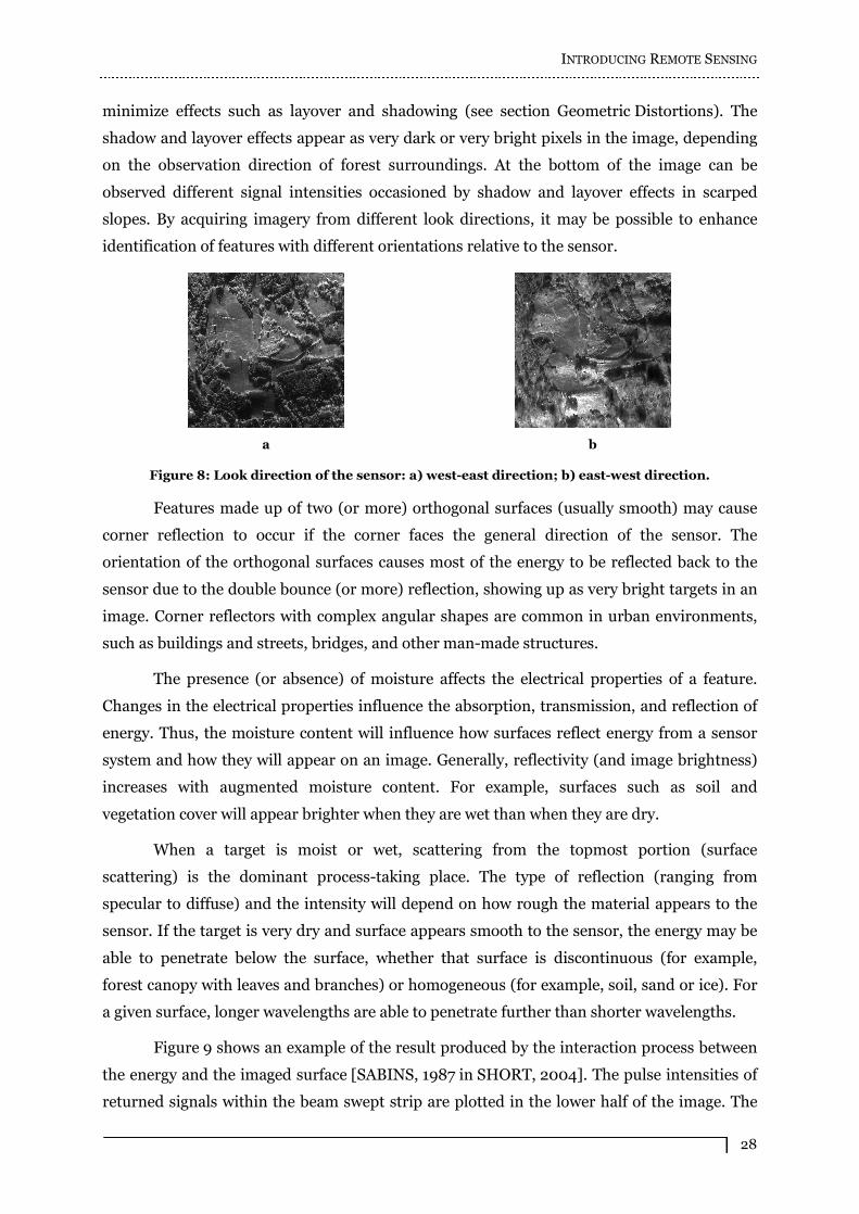
The look direction of the sensor describes the orientation of the transmitted sensor
beam relative to the direction or alignment of linear features on the surface. The look
direction can significantly influence the appearance of features on an image, particularly
when ground features are organized in a linear structure (such as agricultural crops or
mountain ranges). This can be visualized in Figure 8. The agriculture and forest areas at the
top of the figures provide different signal intensities according to the observation direction. If
the look direction is close to perpendicular to the orientation of the feature, then a large
portion of the incident energy will be reflected back to the sensor and the feature will appear
as a brighter tone. If the look direction is more oblique in relation to the feature orientation,
then less energy will be returned to the sensor and the feature will appear darker in tone.
Look direction is important for enhancing the contrast between features in an image. It is
particularly important to have the proper look direction in mountainous regions in order to
INTRODUCING REMOTE SENSING
28
minimize effects such as layover and shadowing (see section Geometric Distortions). The
shadow and layover effects appear as very dark or very bright pixels in the image, depending
on the observation direction of forest surroundings. At the bottom of the image can be
observed different signal intensities occasioned by shadow and layover effects in scarped
slopes. By acquiring imagery from different look directions, it may be possible to enhance
identification of features with different orientations relative to the sensor.
a
b
Figure 8: Look direction of the sensor: a) west-east direction; b) east-west direction.
Features made up of two (or more) orthogonal surfaces (usually smooth) may cause
corner reflection to occur if the corner faces the general direction of the sensor. The
orientation of the orthogonal surfaces causes most of the energy to be reflected back to the
sensor due to the double bounce (or more) reflection, showing up as very bright targets in an
image. Corner reflectors with complex angular shapes are common in urban environments,
such as buildings and streets, bridges, and other man-made structures.
The presence (or absence) of moisture affects the electrical properties of a feature.
Changes in the electrical properties influence the absorption, transmission, and reflection of
energy. Thus, the moisture content will influence how surfaces reflect energy from a sensor
system and how they will appear on an image. Generally, reflectivity (and image brightness)
increases with augmented moisture content. For example, surfaces such as soil and
vegetation cover will appear brighter when they are wet than when they are dry.
When a target is moist or wet, scattering from the topmost portion (surface
scattering) is the dominant process-taking place. The type of reflection (ranging from
specular to diffuse) and the intensity will depend on how rough the material appears to the
sensor. If the target is very dry and surface appears smooth to the sensor, the energy may be
able to penetrate below the surface, whether that surface is discontinuous (for example,
forest canopy with leaves and branches) or homogeneous (for example, soil, sand or ice). For
a given surface, longer wavelengths are able to penetrate further than shorter wavelengths.
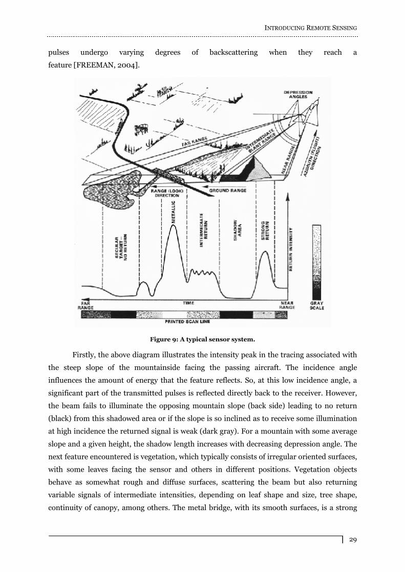
Figure 9 shows an example of the result produced by the interaction process between
the energy and the imaged surface [SABINS, 1987 in SHORT, 2004]. The pulse intensities of
returned signals within the beam swept strip are plotted in the lower half of the image. The
INTRODUCING REMOTE SENSING
29
pulses undergo varying degrees of backscattering when they reach a
feature [FREEMAN, 2004].
Figure 9: A typical sensor system.
Firstly, the above diagram illustrates the intensity peak in the tracing associated with
the steep slope of the mountainside facing the passing aircraft. The incidence angle
influences the amount of energy that the feature reflects. So, at this low incidence angle, a
significant part of the transmitted pulses is reflected directly back to the receiver. However,
the beam fails to illuminate the opposing mountain slope (back side) leading to no return
(black) from this shadowed area or if the slope is so inclined as to receive some illumination
at high incidence the returned signal is weak (dark gray). For a mountain with some average
slope and a given height, the shadow length increases with decreasing depression angle. The
next feature encountered is vegetation, which typically consists of irregular oriented surfaces,
with some leaves facing the sensor and others in different positions. Vegetation objects
behave as somewhat rough and diffuse surfaces, scattering the beam but also returning
variable signals of intermediate intensities, depending on leaf shape and size, tree shape,
continuity of canopy, among others. The metal bridge, with its smooth surfaces, is a strong
INTRODUCING REMOTE SENSING
30
reflector (buildings, with their edges and corners, also tend to behave that way but the nature
of their exterior materials somewhat reduces the returns). The lake, with its smooth surface,
works as a specular reflector to divert most of the signal away from the receiver in this far
range position. Smooth surfaces at near range locations will return more of the signal.
The signal trace shown in Figure 9 represents a single scan line, which is composed of
pixels, each corresponding to a specific area on the ground. The successions of scan lines
produce an image.
2.2.2 REMOTE SENSING SENSORS
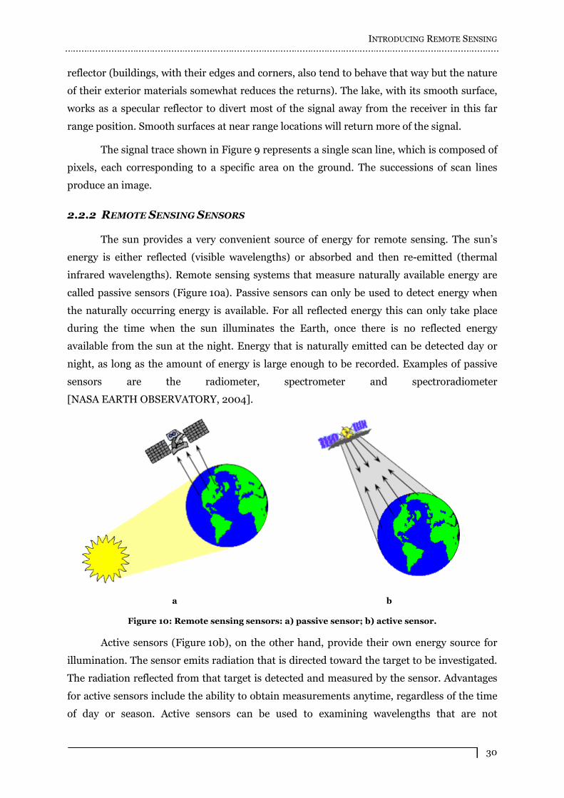
The sun provides a very convenient source of energy for remote sensing. The sun�s
energy is either reflected (visible wavelengths) or absorbed and then re-emitted (thermal
infrared wavelengths). Remote sensing systems that measure naturally available energy are
called passive sensors (Figure 10a). Passive sensors can only be used to detect energy when
the naturally occurring energy is available. For all reflected energy this can only take place
during the time when the sun illuminates the Earth, once there is no reflected energy
available from the sun at the night. Energy that is naturally emitted can be detected day or
night, as long as the amount of energy is large enough to be recorded. Examples of passive
sensors are the radiometer, spectrometer and spectroradiometer
[NASA EARTH OBSERVATORY, 2004].
a
b
Figure 10: Remote sensing sensors: a) passive sensor; b) active sensor.
Active sensors (Figure 10b), on the other hand, provide their own energy source for
illumination. The sensor emits radiation that is directed toward the target to be investigated.
The radiation reflected from that target is detected and measured by the sensor. Advantages
for active sensors include the ability to obtain measurements anytime, regardless of the time
of day or season. Active sensors can be used to examining wavelengths that are not

INTRODUCING REMOTE SENSING
31
sufficiently provided by the sun, such as microwaves, or to have better control of the way a
target is illuminated. However, active systems require the generation of a fairly large amount
of energy to adequately illuminate targets. Different types of active sensors are the radar, the
scatterometer, the LIDAR (LIght Detection And Ranging) and the laser
altimeter [NASA EARTH OBSERVATORY, 2004].
In order for a sensor to collect and record energy reflected or emitted from a target
(element D in Figure 1), it must reside on a stable platform removed from the target being
observed. Platforms for remote sensors may be situated on the ground, on an aircraft or
balloon (or some other platform within the Earth�s atmosphere), or on a spacecraft or
satellite outside of the Earth�s atmosphere. Cost is often a significant factor in choosing
among the various platform options. This research work approaches aerial
platforms [SCHWÄBISCH & MOREIRA, 1999], which are often used to collect very detailed
images and facilitate the collection of data over almost any portion of the Earth�s surface at
almost any time.
There are many types of sensors that are used for remote sensing purposes, such as
LIDAR and radar, among others [NASA OBSERVATORIUM - Resources, 2004]. This
research work approaches the use of microwave-based active radar sensors to collect
data [SCHWÄBISCH & MOREIRA, 1999].
2.2.2.1 THE RADAR
Active microwave sensors are generally divided into two distinct categories: non-
imaging and imaging. Non-imaging microwave sensors include altimeters and
scatterometers. In most cases these are profiling devices that take measurements in one
linear dimension. For the remainder of this research work the focus will be only on imaging
sensors.
The most common form of imaging active microwave sensor is the radar. Radar is an
acronym for RAdio Detection And Ranging [SHORT, 2004].
Radar is essentially a ranging or distance-measuring device. It consists fundamentally
of a transmitter, a receiver, an antenna, and an electronics system to process and record the
data. The transmitter generates successive pulses of microwave (covers the range from
approximately 1 cm to 1 m in wavelength, as can be seen in Figure 4) at regular intervals,
which are focused by the antenna into a beam. The antenna receives a portion of the
transmitted energy reflected from various objects within the illuminated beam. By measuring
the time delay between the transmission of a pulse and the reception of the backscattered
�echo� from different targets, their distance from the radar and thus their location can be
determined. As the sensor platform moves forward, recording and processing of the

INTRODUCING REMOTE SENSING
32
backscattered signals builds up a 2D image of the surface.
Because radar provides its own energy source, images can be acquired day or night.
Moreover, the long wavelengths of microwave radiation enable it to penetrate through clouds
and most rain, being possible to use it in any weather [INPE, 2004].
The microwave region of the spectrum is referenced according to wavelength and
frequency. So longer a wave is, so deeper it can penetrate. This region is quite large and there
are several wavelength ranges or bands commonly used which given code letters during
World War II remain to this day; Figure 4 illustrates them. Two of these bands, currently
more popular, are described bellow:
X-band � this short wave shows typically a high attenuation and is mainly reflected from
the surface or from the top of the vegetation and provides information about the surface
of objects;
P-band � this longest radar wavelengths normally penetrate deep into vegetation and
often also into the ground.
Figure 11 shows two scenes of the same landscape, imaged with different frequencies.
It can be seen how the frequency influences the backscattering. In the X-band scene
(Figure 11a) the agriculture areas can be easily demarcated, and the streets can be identified.
In the P-band scene (Figure 11b) these characteristics are not visible, but the difference
between forests and agriculture areas is more visible. The residential areas are visible in both
scenes.
a
b
Figure 11: Scenes imaged with different wavelengths: a) X-band; b) P-band.
When discussing microwave energy, the polarization of the radiation is also
important. Polarimetry, as its name implies, is an advanced radar research area that involves
discriminating between the polarizations that a radar system is able to transmit and receive.
Polarization refers to the orientation of the electric field. Most radar sensors are designed to

INTRODUCING REMOTE SENSING
33
transmit microwave radiation either horizontally polarized or vertically polarized. Similarly,
the antenna receives either the horizontally or vertically polarized backscattered energy, and
some radar sensors can receive both. The letters H for horizontal, and V for vertical designate
these two polarization states. Thus, there can be four combinations of both transmit and
receive polarizations as follows: HH � for horizontal transmit and horizontal receive, VV �
for vertical transmit and vertical receive, HV � for horizontal transmit and vertical receive,
and VH � for vertical transmit and horizontal receive.
The first two polarization combinations are referred to as like-polarized because the
transmit polarization and the receive polarization are the same. The last two combinations
are referred to as cross-polarized because the transmit and receive polarizations are opposite
of one another. Similar to variations in wavelength, depending on the transmit polarization
and the receive polarization, the radiation will interact with and be backscattered differently
from the surface. Both wavelength and polarization affect how radar sees the surface.
Therefore, radar imagery collected using different polarization and wavelength combinations
may provide different and complementary information about the targets.
Most radar systems transmit microwave radiation in either horizontal or vertical
polarization, and similarly, receive the backscattered signal at only one of these polarizations.
Multi-polarization radars are able to transmit either H or V polarization and receive both the
like- and cross-polarized returns. Polarimetric radars are able to transmit and receive both
horizontal and vertical polarizations. Thus, they are able to receive and process all four
combinations of these polarizations. Each of these �polarization channels� has varying
sensitivities to different surface characteristics and properties. Thus, the availability of multi-
polarization data helps to improve the identification of, and the discrimination between
features [BRANDFASS ET AL., 2000].
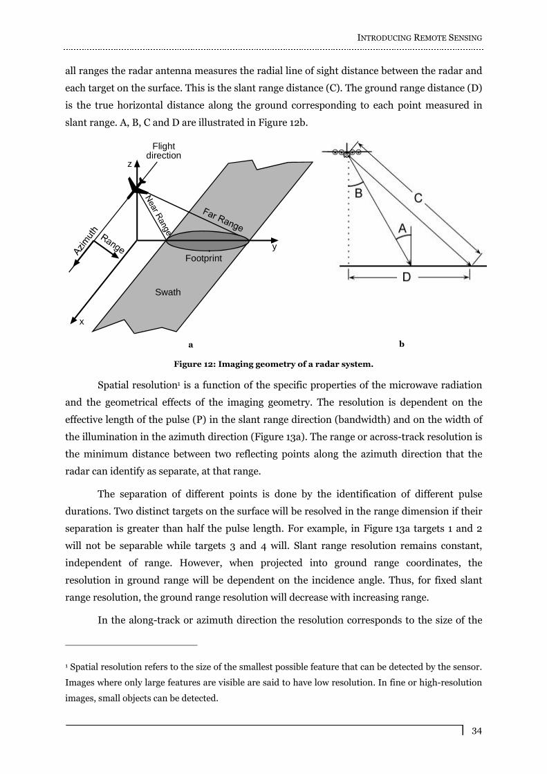
The imaging geometry of a radar system (Figure 12a) consists of a platform that
travels forward in the flight direction with the nadir directly under the platform. The
microwave beam is transmitted obliquely illuminating a swath that is offset from nadir.
Range refers to the across-track dimension perpendicular to the flight direction, while
azimuth refers to the along-track dimension parallel to the flight direction. The portion of the
image swath closest to the nadir-track of the radar platform is called the near range while the
portion of swath farthest from the nadir is called the far range. This side-looking viewing
geometry is typical of imaging radar systems.
The incidence angle (A) is the angle between the radar beam and the ground surface
that increases, moving across the swath from near to far range. The look angle (B) is the angle
at which the radar �looks� at the surface. In the near range, the viewing geometry may be
referred to as being steep, relative to the far range, where the viewing geometry is shallow. At
INTRODUCING REMOTE SENSING
34
all ranges the radar antenna measures the radial line of sight distance between the radar and
each target on the surface. This is the slant range distance (C). The ground range distance (D)
is the true horizontal distance along the ground corresponding to each point measured in
slant range. A, B, C and D are illustrated in Figure 12b.
x
y
z
Flightdirection
Footprint
Swath
a b
Figure 12: Imaging geometry of a radar system.
Spatial resolution1 is a function of the specific properties of the microwave radiation
and the geometrical effects of the imaging geometry. The resolution is dependent on the
effective length of the pulse (P) in the slant range direction (bandwidth) and on the width of
the illumination in the azimuth direction (Figure 13a). The range or across-track resolution is
the minimum distance between two reflecting points along the azimuth direction that the
radar can identify as separate, at that range.
The separation of different points is done by the identification of different pulse
durations. Two distinct targets on the surface will be resolved in the range dimension if their
separation is greater than half the pulse length. For example, in Figure 13a targets 1 and 2
will not be separable while targets 3 and 4 will. Slant range resolution remains constant,
independent of range. However, when projected into ground range coordinates, the
resolution in ground range will be dependent on the incidence angle. Thus, for fixed slant
range resolution, the ground range resolution will decrease with increasing range.
In the along-track or azimuth direction the resolution corresponds to the size of the
1 Spatial resolution refers to the size of the smallest possible feature that can be detected by the sensor.
Images where only large features are visible are said to have low resolution. In fine or high-resolution
images, small objects can be detected.

INTRODUCING REMOTE SENSING
35
antenna footprint on the ground (Figure 13b). The beam width (A) is a measure of the width
of the illumination pattern. As the radar illumination propagates to increasing distance from
the sensor, the azimuth resolution becomes coarser. In Figure 13b, targets 1 and 2 in the near
range would be separable, but targets 3 and 4 at further range would not. The radar beam
width is inversely proportional to the antenna length, which means that a longer antenna will
produce a narrower beam and finer resolution.
a
b
Figure 13: Resolution: a) range resolution; b) azimuth resolution.
Finer range resolution can be achieved by using a shorter pulse length, what can be
done within certain engineering design restrictions. Finer azimuth resolution can be achieved
increasing the antenna length. However, the actual length of the antenna is limited by what
can be carried on an airborne platform.
Radar antennas on aircrafts are usually mounted on the underside of the platform so
as to direct their beam to the side of the airplane in a direction normal to the flight path. For
aircraft, this mode of operation is implied in the acronym SLAR, for Side Looking Airborne
Radar.
There are two types of SLAR systems: the Real Aperture Radar (RAR) and the SAR. A
real aperture system, the first microwave imaging system used, operates with a long (about 5-
6 m) antenna and uses its length to obtain the desired resolution in the azimuth direction.
The azimuth resolution in RAR systems is directly proportional to the distance between the
antenna and the target, and inversely proportional to the wavelength used by the antenna.
Thus, in order to obtain a better azimuth resolution, the distance between radar and target
must be reduced, or the length of the antenna must be increased. This is practically not
possible, once to reach an azimuth resolution of 0.5 m with a wavelength of about 3 cm it
would be necessary a 180 m long antenna. The SAR is described next.
INTRODUCING REMOTE SENSING
36
2.2.2.2 THE SYNTHETIC APERTURE RADAR
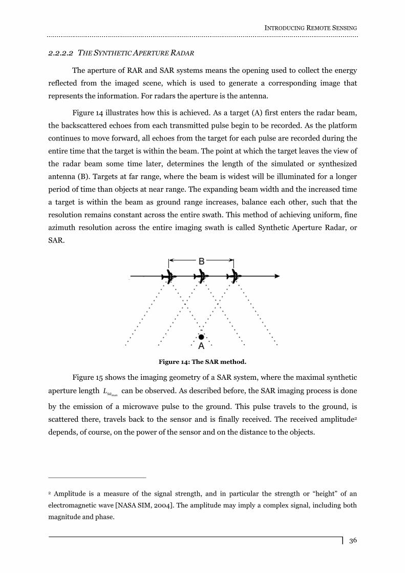
The aperture of RAR and SAR systems means the opening used to collect the energy
reflected from the imaged scene, which is used to generate a corresponding image that
represents the information. For radars the aperture is the antenna.
Figure 14 illustrates how this is achieved. As a target (A) first enters the radar beam,
the backscattered echoes from each transmitted pulse begin to be recorded. As the platform
continues to move forward, all echoes from the target for each pulse are recorded during the
entire time that the target is within the beam. The point at which the target leaves the view of
the radar beam some time later, determines the length of the simulated or synthesized
antenna (B). Targets at far range, where the beam is widest will be illuminated for a longer
period of time than objects at near range. The expanding beam width and the increased time
a target is within the beam as ground range increases, balance each other, such that the
resolution remains constant across the entire swath. This method of achieving uniform, fine
azimuth resolution across the entire imaging swath is called Synthetic Aperture Radar, or
SAR.
Figure 14: The SAR method.
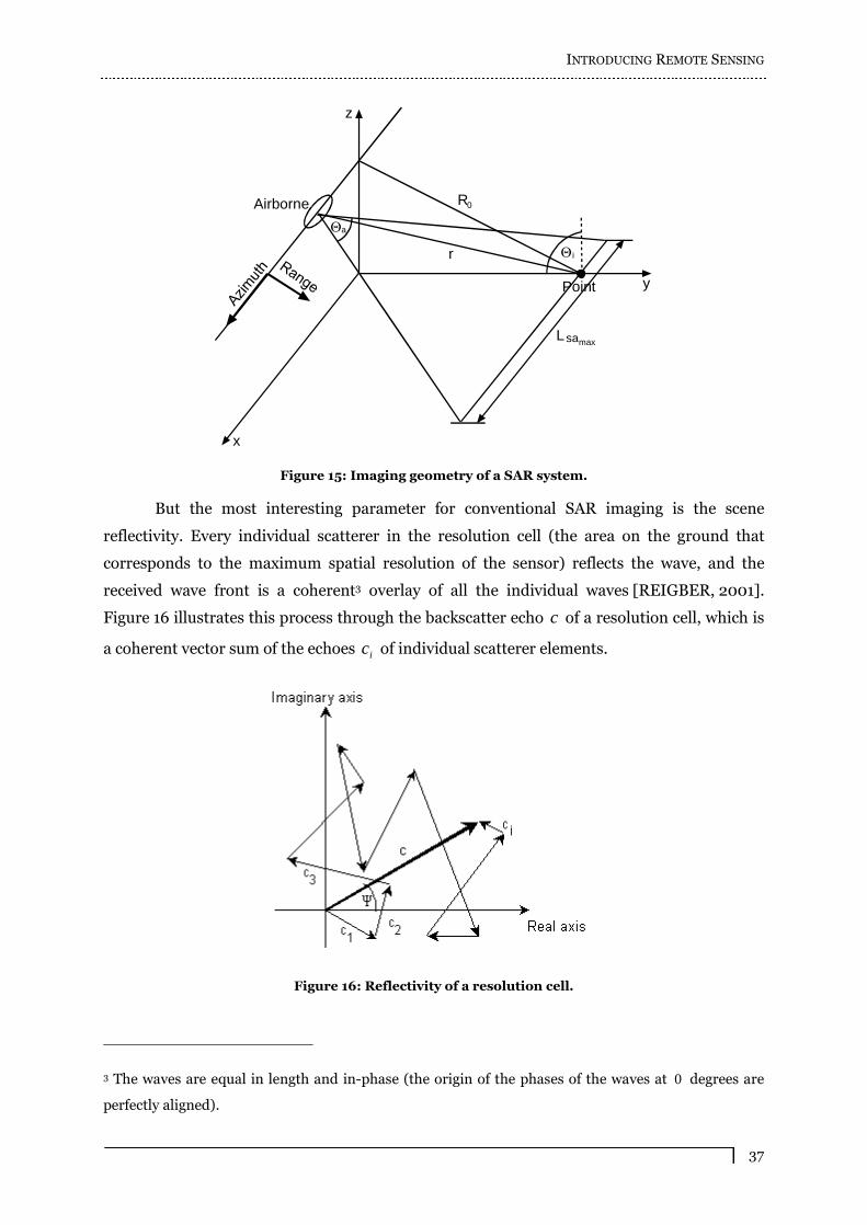
Figure 15 shows the imaging geometry of a SAR system, where the maximal synthetic
aperture length maxsaL can be observed. As described before, the SAR imaging process is done
by the emission of a microwave pulse to the ground. This pulse travels to the ground, is
scattered there, travels back to the sensor and is finally received. The received amplitude2
depends, of course, on the power of the sensor and on the distance to the objects.
2 Amplitude is a measure of the signal strength, and in particular the strength or �height� of an
electromagnetic wave [NASA SIM, 2004]. The amplitude may imply a complex signal, including both
magnitude and phase.
INTRODUCING REMOTE SENSING
37
x
y
r
z
Airborne R0
a
i
Point
Lsamax
Figure 15: Imaging geometry of a SAR system.
But the most interesting parameter for conventional SAR imaging is the scene
reflectivity. Every individual scatterer in the resolution cell (the area on the ground that
corresponds to the maximum spatial resolution of the sensor) reflects the wave, and the
received wave front is a coherent3 overlay of all the individual waves [REIGBER, 2001].
Figure 16 illustrates this process through the backscatter echo c of a resolution cell, which is
a coherent vector sum of the echoes ic of individual scatterer elements.
Figure 16: Reflectivity of a resolution cell.
3 The waves are equal in length and in-phase (the origin of the phases of the waves at 0 degrees are
perfectly aligned).

INTRODUCING REMOTE SENSING
38
The SAR system overcomes the RAR system problems mentioned above and is
designated to achieve high resolutions with small antennas over long distances. The synthetic
aperture of SAR allows a higher spatial resolution in azimuth direction, once it is only
dependent from the size of the real antenna, and not from the wavelength used or the
distance between the sensor and the target. As much as the distance increases, as much
increases the length of the synthetic aperture. The resolution in range direction is realized
through the measure of the sent pulse length; this resolution can be increased through the
shortening of the pulse length [MOREIRA, 1992].
The process of using a synthetic aperture leads up to the problem, especially severe if
the observed area has strong topography, that two points can have the same range distance to
the sensor, but are seen under a different look angle. In this case the radar echo arrives at the
same time at the sensor, and they cannot be separately identified. No height information and
no elevation angle resolution are obtained. Figure 17 illustrates the imaging principle of a
SAR system. Notice that P and 'P cannot be separately identified, because their identical
distance from the sensor S .
r
P''
h
S
r'
P
P'
Height
Range
r''
Figure 17: Imaging principle of a SAR system.
This problem took to the implementation of another approach: the Interferometric
Synthetic Aperture Radar (InSAR).
2.2.2.3 THE INTERFEROMETRIC SYNTHETIC APERTURE RADAR
Interference, the interaction of light waves, is used to measure distances and angles
precisely. The word interferometry illustrates this: interfere + measure = interfer-o-
metry [NASA SIM, 2004].
The InSAR (Interferometric Synthetic Aperture Radar) system applies a different
method as the SAR system to realize the range resolution. This method is used in order to

INTRODUCING REMOTE SENSING
39
solve the problem of the SAR imaging principle that cannot identify different points that are
at the same distance from the sensor. A second sensor position 2S is used spatially separated
from the first sensor position 1S , in order to resolve the ambiguity occurred when two
different points at different positions but with identical distance from the sensor occur.
Figure 18 illustrates this principle, and shows that different points with different heights have
different distances to the sensor positions 1S and 2S .
h
S1
P
P'
Height
Range
S2
r2'
r2
r1
r1'
Figure 18: Imaging principle of an InSAR system.
Interferometry relies on being able to measure a property of electromagnetic waves
called phase [REIGBER, 2004]. Suppose there are two waves (Figure 19) with the exact same
wavelength and frequency traveling along in space, but the starting point of one is offset
slightly from the other. The offset between matching points on these two waves (A) is called
the phase difference. The phase information of the two image data files, acquired by the two
sensors from the same scene, is superimposed.
Figure 19: Phase difference of two electromagnetic waves.
The image phase has two parts, a deterministic one due to the sensor-scatterer
distance and a random object phase, which results from the scattering process on the object.
If the same object is observed two times from nearly the same position, it can be assumed
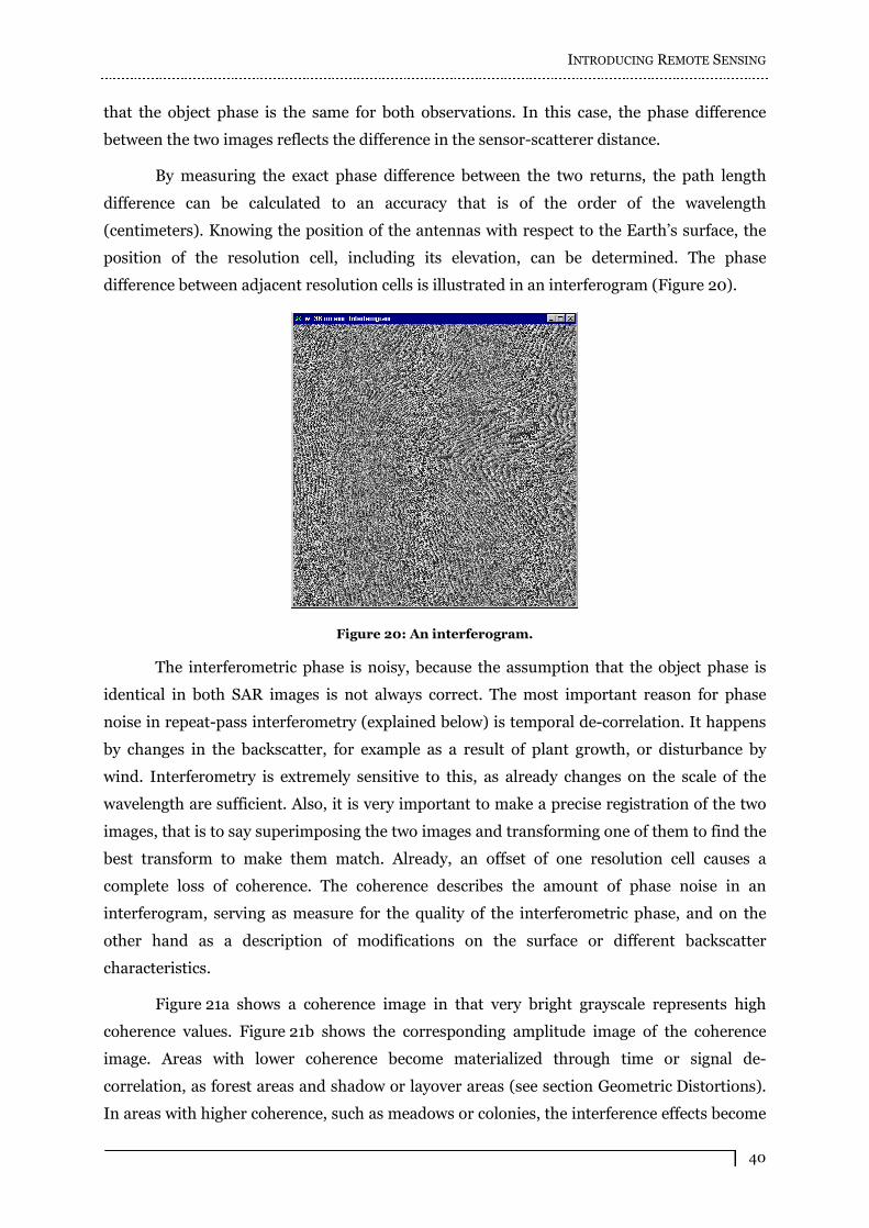
INTRODUCING REMOTE SENSING
40
that the object phase is the same for both observations. In this case, the phase difference
between the two images reflects the difference in the sensor-scatterer distance.
By measuring the exact phase difference between the two returns, the path length
difference can be calculated to an accuracy that is of the order of the wavelength
(centimeters). Knowing the position of the antennas with respect to the Earth�s surface, the
position of the resolution cell, including its elevation, can be determined. The phase
difference between adjacent resolution cells is illustrated in an interferogram (Figure 20).
Figure 20: An interferogram.
The interferometric phase is noisy, because the assumption that the object phase is
identical in both SAR images is not always correct. The most important reason for phase
noise in repeat-pass interferometry (explained below) is temporal de-correlation. It happens
by changes in the backscatter, for example as a result of plant growth, or disturbance by
wind. Interferometry is extremely sensitive to this, as already changes on the scale of the
wavelength are sufficient. Also, it is very important to make a precise registration of the two
images, that is to say superimposing the two images and transforming one of them to find the
best transform to make them match. Already, an offset of one resolution cell causes a
complete loss of coherence. The coherence describes the amount of phase noise in an
interferogram, serving as measure for the quality of the interferometric phase, and on the
other hand as a description of modifications on the surface or different backscatter
characteristics.
Figure 21a shows a coherence image in that very bright grayscale represents high
coherence values. Figure 21b shows the corresponding amplitude image of the coherence
image. Areas with lower coherence become materialized through time or signal de-
correlation, as forest areas and shadow or layover areas (see section Geometric Distortions).
In areas with higher coherence, such as meadows or colonies, the interference effects become

INTRODUCING REMOTE SENSING
41
insignificant.
a
b
Figure 21: Coherence of an imaged surface: a) coherence scene; b) X-band SAR scene.
The information contained in an interferogram can be used to derive topographic
information and produce 3D imagery of terrain height, in other words, DEMs (Figure 22).
Figure 22: 2D and 3D views of the terrain height.
Figure 23 illustrates the measure principle used by the InSAR system. The baseline B
represents the distance between the two sensor positions 1S and 2S , which define the
imaging geometry for point P through the angles 1È and 2È , and the slant distances 1r and
2r . The distance difference rÄ is measured through the definition of the phase difference,
and is dependent of the imaging geometry and mainly of the target point height h .
Two different imaging processes can be performed, applying InSAR: the single-pass
interferometry and the repeat-pass interferometry. The first uses a second antenna on the
sensor platform, sending the signal with one of the antennas and receiving the signal with
two antennas. Its advantage is that the observations occur practically at the same time, so
that the temporal de-correlation is not applicable. The second one illuminates twice the
target, using slightly displaced flight tracks. This process leads to stronger de-correlations,

INTRODUCING REMOTE SENSING
42
thus the time interval between the observations or the inaccurate flight track repetition.
Motion compensation algorithms are used to minimize the inaccuracy provoked by flight
instability [MOREIRA, 1992].
P
h
B
r1
r2
S1
S2
Reference surface Terrain
1
2
r
Figure 23: Measure principle of an InSAR system.
SAR interferometry may also be used to measure surface motion (e.g., ocean
currents). In this case the antenna positions are separated in the azimuth direction.
An important example of an InSAR sensor is the AeS-1. This radar started to be
designed and constructed in the beginning of 1996 by Aero-Sensing Radarsysteme
GmbH [AERO-SENSING, 2001], a leading German company in the development and use of
radar and InSAR technology to produce high precision DEMs (actually Aero-Sensing
integrates the Canadian company Intermap Technologies Corp. [INTERMAP, 2004]). AeS-1
can produce X-band and P-band scenes, and is flown on an airborne platform. A detailed
description of the AeS-1 system can be found in [SCHWÄBISCH & MOREIRA, 1999].
2.2.3 INTERFEROMETRIC SYNTHETIC APERTURE RADAR PROCESSING
The interferometric processing of SAR data allows the extraction of knowledge about
the topography of the imaged terrain, what is to say that the terrain height can be estimated
(element E in Figure 1) [SCHWÄBISCH, 1995].
Figure 24 shows a block diagram of a processing chain, in order to process two
complex SAR scenes into a DEM. This SAR and InSAR processor has been developed and
applied by Aero-Sensing Radarsysteme GmbH. In order to understand the main steps to be
followed to generate a DEM, they will be briefly described next. For more information about
generation of high precision DEMs, refer to [WIMMER ET AL., 2000].
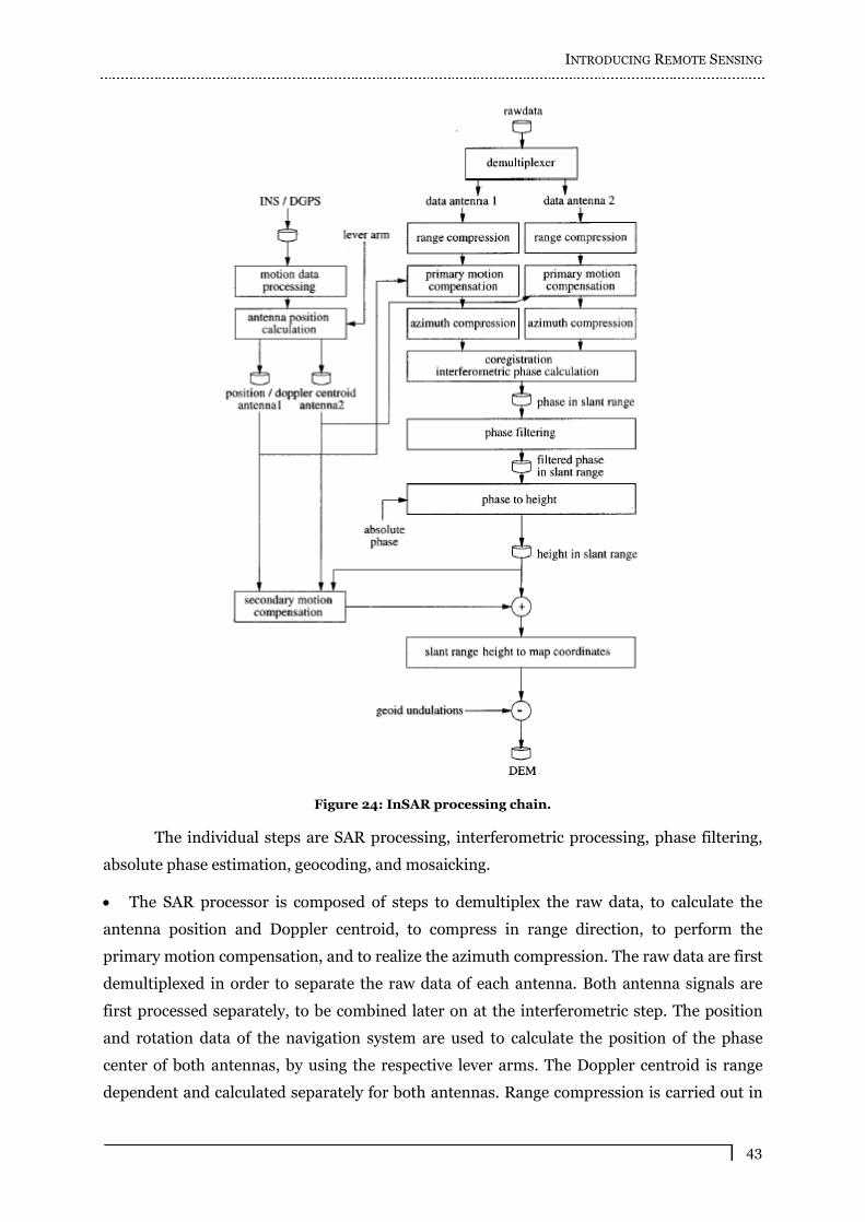
INTRODUCING REMOTE SENSING
43
Figure 24: InSAR processing chain.
The individual steps are SAR processing, interferometric processing, phase filtering,
absolute phase estimation, geocoding, and mosaicking.
The SAR processor is composed of steps to demultiplex the raw data, to calculate the
antenna position and Doppler centroid, to compress in range direction, to perform the
primary motion compensation, and to realize the azimuth compression. The raw data are first
demultiplexed in order to separate the raw data of each antenna. Both antenna signals are
first processed separately, to be combined later on at the interferometric step. The position
and rotation data of the navigation system are used to calculate the position of the phase
center of both antennas, by using the respective lever arms. The Doppler centroid is range
dependent and calculated separately for both antennas. Range compression is carried out in
INTRODUCING REMOTE SENSING
44
the frequency domain and uses the chirp replica as a reference function. Azimuth
compression is performed using a hybrid correlation algorithm that uses a frequency domain
fast correlation in the azimuth direction, with a time domain convolution operation in the
range dimension. The output of the azimuth compression is a single look complex image.
After SAR focusing, two single look complex datasets enter the interferometric processor.
Its task is to extract each target�s phase signature from both channels and combine them
coherently to form an unwrapped phase difference image (interferogram) with the best
possible signal to noise ratio. The basic processing steps are image coregistration,
interferogram formation, and phase unwrapping, which are implemented using standard
algorithms.
The phase filtering step aims to prepare the raw interferometric phase in such a form that
the resulting DEM is as close as possible to the real topography. The raw interferometric
phase contains artifacts and noisy areas that should be filtered. The filter used in this step has
to be developed according to the terrain type.
The phase offset for estimating the absolute phase is calculated based on precise
reference points, by forward or backward geocoding. Following this calibration step, a
secondary motion compensation has to be done since the primary motion compensation was
carried out without considering the topography. This compensation is performed converting
the interferometric phase into height, compensating remaining height errors and converting
the improved slant range height image into a cartographic reference system.
Solving standard range/Doppler equations and the ellipsoid equation carries out the
derivation of geocoded height information, what is to say, terrain elevation data projected
over the Earth�s surface.
The final elevation model is composed by mosaicking and averaging a stack of individual
elevation layers, using weights in order to further improve the height accuracy.
Figure 25 illustrates some results produced by the use of the processing chain to
generate the Etna Volcano DEM: a) and b) single look complex images output by the SAR
processor; c) interferogram showing the phase difference; d) absolute phase determined by
the phase unwrapping process to resolve the phase ambiguities (qualitative description of the
terrain); e) phase conversion into terrain height; f) geocoding.

INTRODUCING REMOTE SENSING
45
a
b
c
d
e
f
Figure 25: Results produced by different steps of an InSAR processing chain.

INTRODUCING REMOTE SENSING
46
2.3 FINAL REMARKS
This thesis proposes a methodology to enhance DEMs through the correction of their
inaccurate elevation values. The raw data used to generate the DEMs utilized by this work to
demonstrate the applicability of the proposed methodology are collected using an airborne
platform with a radar sensor mounted on the underside of it. This radar is an InSAR sensor
and has two simultaneously operable antennas. It can produce X-band and P-band scenes,
what makes it a powerful sensor able to produce DEMs that represent both the top elevation
of objects, and the ground elevation excluding forest vegetation. The processing chain used to
generate the height models uses an interferometric method that produces products with a
global precision of the order of centimeters. Although these results are very good, there exist
local areas in the generated DEMs where the data are not accurate, which need to be
corrected in order that the data may be reliably applied.
The seven elements that compose the remote sensing process were explained partially
during this chapter (from element 1 to 5). Element 6 tackles the subject of interpretation and
analysis of the processed DEMs. It will be explained in chapter 4, where some relevant
visualization and exploration techniques, that currently are applied to support the user to
extract information from the models, are described. Element 7, the application of the
extracted information, can be seen as a motivation for this work: the user, in order to apply
accurately the information extracted from the DEM, has to have in hand a model as precise as
possible.

CHAPTER 3
DIGITAL ELEVATION MODELS
3.1 INTRODUCTION TO THE CHAPTER
The DEM is the application used to validate the methodology proposed by this thesis.
This chapter starts reviewing the main concepts related to it.
An important subject tackled during this description is the presence of errors in DEM
data. As described in the previous chapter, DEMs are generated from raw data collected, for
example, by a radar sensor. This sensor performs distance measurements to obtain
information about the height of an imaged terrain. Therefore, an error, in the context of this
thesis, is the departure of a measurement from its true value. Why errors occur, and the kinds
of errors that exist are topics explained in detail.
Research works that focus on the identification, quantification and reduction of
different kinds of errors in DEMs generated from data collected by different sensors, coupled
on different platforms, are described. While this text is not meant to be an exhaustive review
of the literature about these themes, it introduces the major researches available. This
information should help verifying what makes the methodology proposed by this thesis stand
out from the existing ones, being more effective.
3.2 CONCEPTS OF DIGITAL ELEVATION MODELS
A Digital Elevation Model (DEM) can be defined as �a regular gridded matrix
representation of the continuous variation of relief over space� [WOOD, 1996].
In order to represent digitally a terrain, it can be described through a height map,
taking for each point the height of the terrain over this point. Formally, the height map is a
function RRUf 2: , yxfz , , where yx, are the coordinates of the plane and z is the
corresponding height. A method to represent the terrain consists of taking a grid of points
ji yx , ni ,,1 , mj ,,1 in the function domain. For each vertex ji yx , of the grid the
value of the function jiij yxfz , is taken, having the representation of the terrain by the
matrix of heights ijz [GOMES & VELHO, 1998].
An image is represented in the same way as the terrain representation described
above. For instance, observe a black and white image, that has only the colors black and
white, and degrees of gray. In this case, to each degree of gray it is associated a number in the
interval 1,0 , where 0 represents the black color and 1 represents the white color. A black
DIGITAL ELEVATION MODELS
48
and white image is a function RRUf 2: , yxfz , which associates to each point yx,
the value z of the corresponding degree of gray. In the context of this thesis, the relation
between the representation of an image and a DEM is relevant because
filters [GOMES & VELHO, 1994], commonly used with images, as well as some analysis
techniques, may be used to edit and analyze DEM datasets.
DEMs are generated based on data collected through an imaging process. Depending
on the type of remote sensing system applied to obtain these data, they can acquire
information about the imaged terrain surface (with different orders of precision, anywhere
from centimeters to meters) or about the surface of objects over the terrain, such as
vegetation or man-made objects (houses, fences, vehicles, to name only a few). Sometimes
different terminologies are used for models that represent ground surface (Digital Ground
Model DGM or Digital Terrain Model DTM) and for models that represent the objects
over the terrain surface, where they exist (Digital Surface Model DSM or Digital Elevation
Model DEM); in this thesis the term DEM is used for both kinds of models. Currently
InSAR systems, which are the ones used to collect the DEMs applied by this thesis, can
provide data for generation of DEMs that have the accuracy of few
centimeters [WIMMER ET AL., 2000; ORBISAT, 2004].
After the collection, raw data have to be processed using sophisticated algorithms in
order to produce DEMs. High resolution DEMs can be used in different applications, and
become especially relevant to supply information about regions where there are no detailed,
precise and updated topographic maps available.
3.3 CHARACTERIZING A DIGITAL ELEVATION MODEL
Techniques and issues are considered surrounding the characterization of DEMs.
Non-spatial statistical descriptors include the moments of the distribution and the accuracy
statistics. Spatial measures include experimental variograms (semivariograms) and spatial
autocorrelation.
3.3.1 NON-SPATIAL DIGITAL ELEVATION MODEL CHARACTERIZATION
Non-spatial DEM characterization can be performed using moment statistics and the
Moran�s I [CLIFF & ORD, 1981 in WOOD, 1996] accuracy statistic. These methods are
described below.
3.3.1.1 MOMENT STATISTICS
Moment descriptions are the conventional descriptions of a frequency distribution
that include measures of central tendency and dispersion (mean, standard deviation,
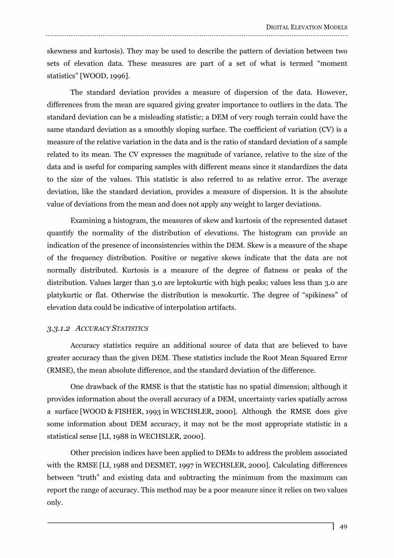
DIGITAL ELEVATION MODELS
49
skewness and kurtosis). They may be used to describe the pattern of deviation between two
sets of elevation data. These measures are part of a set of what is termed �moment
statistics� [WOOD, 1996].
The standard deviation provides a measure of dispersion of the data. However,
differences from the mean are squared giving greater importance to outliers in the data. The
standard deviation can be a misleading statistic; a DEM of very rough terrain could have the
same standard deviation as a smoothly sloping surface. The coefficient of variation (CV) is a
measure of the relative variation in the data and is the ratio of standard deviation of a sample
related to its mean. The CV expresses the magnitude of variance, relative to the size of the
data and is useful for comparing samples with different means since it standardizes the data
to the size of the values. This statistic is also referred to as relative error. The average
deviation, like the standard deviation, provides a measure of dispersion. It is the absolute
value of deviations from the mean and does not apply any weight to larger deviations.
Examining a histogram, the measures of skew and kurtosis of the represented dataset
quantify the normality of the distribution of elevations. The histogram can provide an
indication of the presence of inconsistencies within the DEM. Skew is a measure of the shape
of the frequency distribution. Positive or negative skews indicate that the data are not
normally distributed. Kurtosis is a measure of the degree of flatness or peaks of the
distribution. Values larger than 3.0 are leptokurtic with high peaks; values less than 3.0 are
platykurtic or flat. Otherwise the distribution is mesokurtic. The degree of �spikiness� of
elevation data could be indicative of interpolation artifacts.
3.3.1.2 ACCURACY STATISTICS
Accuracy statistics require an additional source of data that are believed to have
greater accuracy than the given DEM. These statistics include the Root Mean Squared Error
(RMSE), the mean absolute difference, and the standard deviation of the difference.
One drawback of the RMSE is that the statistic has no spatial dimension; although it
provides information about the overall accuracy of a DEM, uncertainty varies spatially across
a surface [WOOD & FISHER, 1993 in WECHSLER, 2000]. Although the RMSE does give
some information about DEM accuracy, it may not be the most appropriate statistic in a
statistical sense [LI, 1988 in WECHSLER, 2000].
Other precision indices have been applied to DEMs to address the problem associated
with the RMSE [LI, 1988 and DESMET, 1997 in WECHSLER, 2000]. Calculating differences
between �truth� and existing data and subtracting the minimum from the maximum can
report the range of accuracy. This method may be a poor measure since it relies on two values
only.

DIGITAL ELEVATION MODELS
50
Another measure of accuracy is the mean absolute difference between interpolated
and true values and the standard deviation of these differences. The mean absolute difference
is a measure of the surface �shift� and the standard deviation represents the measure of
dispersion of this shift. Therefore the accuracy can be reported as mean absolute difference
the standard deviation of difference [LI, 1988 in WECHSLER, 2000].
3.3.2 SPATIAL DIGITAL ELEVATION MODEL CHARACTERIZATION
Several authors have suggested that the errors distribution in elevation models will
show some form of spatial patterning [WOOD & FISHER, 1993 and MONCKTON, 1994
in WOOD, 1996]. In order to test this idea, it is necessary to provide descriptions of the
spatial error pattern.
Statistical analyses that capture spatial relationships within the DEM include
quantification of the distance of spatial dependence through the variogram and
quantification of spatial autocorrelation.
3.3.2.1 THE VARIOGRAM
The variogram is calculated by taking every data point in a DEM, and plotting the
squared difference between all pairs of points against the separation distance between the
points. The mean square elevation difference depends on the horizontal distance between
two selected points. The semi-variogram is a smooth line through these points. Analysis of
the semi-variogram provides information about the spatial characteristics of the dataset and
is often used to explore spatial interdependence [KITANIDIS, 1997 in WECHSLER, 2000].
3.3.2.2 SPATIAL AUTOCORRELATION
A characteristic of geographic data is that values at points close together in space are
more likely to be similar than values farther apart. This characteristic of spatial data is
referred to as spatial autocorrelation.
One method used to measure the degree to which values in a cell are similar to
surrounding values is the Moran�s I statistic which ranges from 1 to 1 . A value of 1
indicates that close data points have dissimilar values; zero indicates no spatial ordering or
randomness and 1 indicates high spatial ordering. Moran�s I statistic uses a global mean of
the surface and therefore is insensitive to local means and
variances [MONCKTON, 1994 in WECHSLER, 2000].
3.4 ERRORS IN DIGITAL ELEVATION MODELS
Once the imaging process of the surface and the raw data processing method are very

DIGITAL ELEVATION MODELS
51
complex and depend on a series of combined parameters (airborne parameters, radar
parameters, data correlation), several error components may be added to the data.
Taylor [TAYLOR, 1997 in WECHSLER, 2000] makes the following statement about
the word error: �In science, the word error does not carry the usual connotations of the
term mistake or blunder. Error in a scientific measurement means the inevitable
uncertainty that attends all measurements. As such, errors are not mistakes; you cannot
eliminate them by being very careful. The best you can hope to do is ensure that errors are
as small as reasonably possible and to have a reliable estimate of how large they are�.
Error is a measurement departure from a true value. Often, in geographic analysis or
analysis of complex natural systems using spatial data, it is not possible to know or to have
access to true values. The lack of knowledge about the reliability of a measurement in its
representation of the true value is referred to as uncertainty. Unfortunately the exact nature
and location of errors cannot be precisely determined.
Sources of possible errors in DEM datasets include the following, as specified by the
USGS [USGS, 1997] and [BURROUGH, 1986 and WISE, 1998 in WECHSLER, 2000]:
1. blunders: vertical errors associated with the data collection process; they are an
indication that this process has deteriorated beyond the level of simple systematic or
random errors. Blunders are mistakes caused by transposed numeric values, erroneous
correlations, careless observations, among others. Malfunctioning of the equipment can
also cause them. Observations affected by this kind of errors are useless, and are
generally identified and removed prior to data release;
2. systematic errors: introduced by systems and/or procedures used in the data collection
and DEM generation processes. These errors follow fixed patterns that can cause bias or
artifacts in the final DEM product, which need not to be constant in space. Typical
systematic errors include vertical elevation shifts, fictitious features such as phantom
tops, or ridges, and improper interpretation of terrain surfaces due to the effects of trees,
buildings and shadows;
3. random errors: these errors are of a purely random nature and completely unpredictable.
They remain in the data after blunders and systematic errors are removed, and result
from accidental and unknown combinations of causes beyond the control of the observer.
Although all three types may be reduced in magnitude by technique refinements, they
cannot be completely eliminated [USGS, 1997]. It is impossible to obtain information about
the exact source and amount of error in a particular DEM. Such an undertaking would
involve, for example, field measurements over large areas; even if physically possible, it is
subject to errors. Due to this fact, researchers make the assumption that specific errors

DIGITAL ELEVATION MODELS
52
within DEMs cannot be known and therefore the elevation model is replete with
uncertainty [WECHSLER, 2000; WOOD, 1996].
Therefore, the present research makes the assumption that supporting DEM expert
users with powerful 3D interfaces to visualize, explore and analyze data to identify and
quantify errors in DEMs, and next to edit these error data, can reduce considerable the
amount of errors in the models. Thus, enhancing the DEMs and reducing uncertainty.
3.4.1 GEOMETRIC DISTORTIONS
As explained before, any DEM is subject to some form of systematic errors, depending
on the manner in which the data are acquired. This problem is inherent in remote sensing, as
attempting to accurately represent the 3D surface of the Earth as a 2D image. Geometric
distortions are one example and constitute a severe error component in DEMs. These errors
may be due to a variety of factors, such as the perspective of the sensor optics, the terrain
relief, the motion of the scanning system, the motion and (in)stability of the platform, the
platform altitude and velocity, the curvature and rotation of the Earth, to name only a few.
During the processing of the raw data several algorithms are applied that remove total
or partially some of these errors. But, it is important to note that these correction procedures
are not sufficient to produce precise DEMs.
3.4.1.1 SLANT RANGE SCALE DISTORTION
Slant range scale distortion (Figure 26) occurs because the radar is measuring the
distance along the ground. This results in a varying image scale, moving from near to far
range. Although targets A1 and B1 are the same size on the ground, their apparent
dimensions in slant range (A2 and B2) are different. This causes targets in the near range to
appear compressed relative to the far range.
Figure 26: Slant range scale distortion.
Using trigonometry, ground range distance can be calculated from the slant range
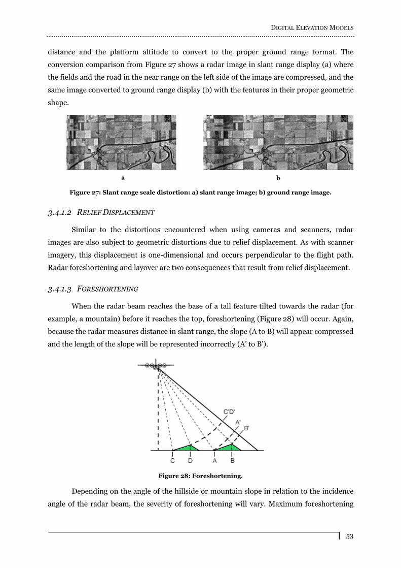
DIGITAL ELEVATION MODELS
53
distance and the platform altitude to convert to the proper ground range format. The
conversion comparison from Figure 27 shows a radar image in slant range display (a) where
the fields and the road in the near range on the left side of the image are compressed, and the
same image converted to ground range display (b) with the features in their proper geometric
shape.
a
b
Figure 27: Slant range scale distortion: a) slant range image; b) ground range image.
3.4.1.2 RELIEF DISPLACEMENT
Similar to the distortions encountered when using cameras and scanners, radar
images are also subject to geometric distortions due to relief displacement. As with scanner
imagery, this displacement is one-dimensional and occurs perpendicular to the flight path.
Radar foreshortening and layover are two consequences that result from relief displacement.
3.4.1.3 FORESHORTENING
When the radar beam reaches the base of a tall feature tilted towards the radar (for
example, a mountain) before it reaches the top, foreshortening (Figure 28) will occur. Again,
because the radar measures distance in slant range, the slope (A to B) will appear compressed
and the length of the slope will be represented incorrectly (A� to B�).
Figure 28: Foreshortening.
Depending on the angle of the hillside or mountain slope in relation to the incidence
angle of the radar beam, the severity of foreshortening will vary. Maximum foreshortening
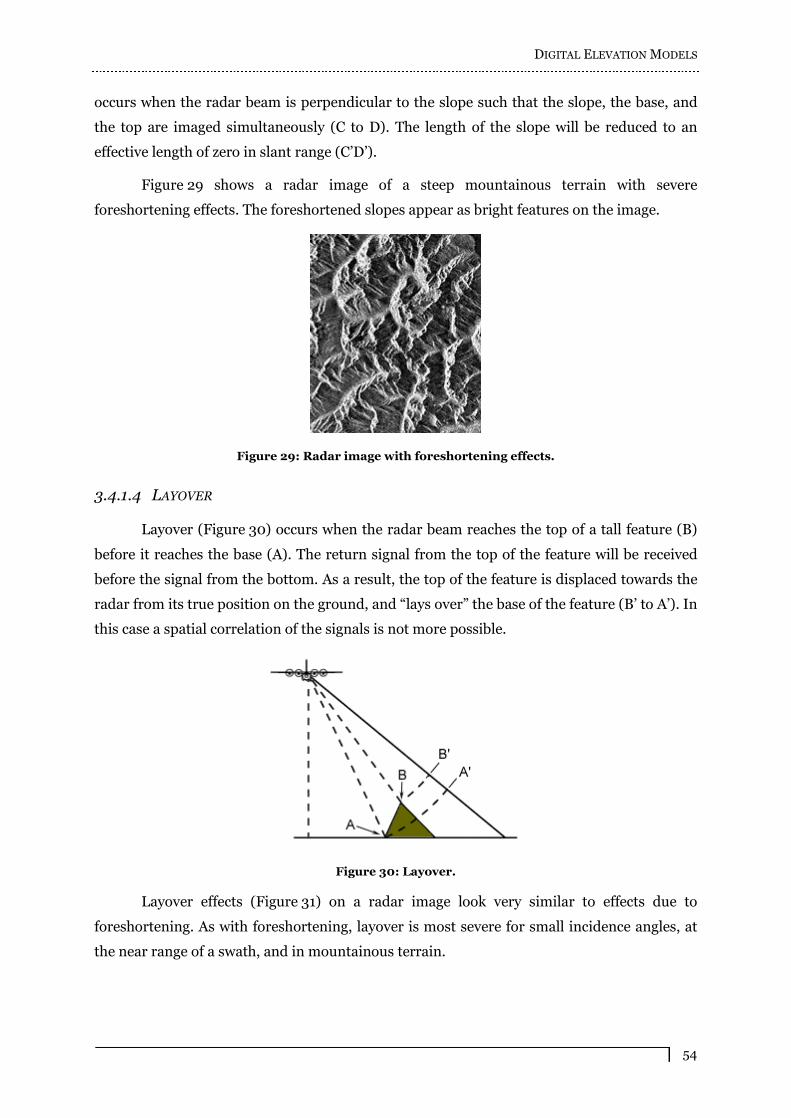
DIGITAL ELEVATION MODELS
54
occurs when the radar beam is perpendicular to the slope such that the slope, the base, and
the top are imaged simultaneously (C to D). The length of the slope will be reduced to an
effective length of zero in slant range (C�D�).
Figure 29 shows a radar image of a steep mountainous terrain with severe
foreshortening effects. The foreshortened slopes appear as bright features on the image.
Figure 29: Radar image with foreshortening effects.
3.4.1.4 LAYOVER
Layover (Figure 30) occurs when the radar beam reaches the top of a tall feature (B)
before it reaches the base (A). The return signal from the top of the feature will be received
before the signal from the bottom. As a result, the top of the feature is displaced towards the
radar from its true position on the ground, and �lays over� the base of the feature (B� to A�). In
this case a spatial correlation of the signals is not more possible.
Figure 30: Layover.
Layover effects (Figure 31) on a radar image look very similar to effects due to
foreshortening. As with foreshortening, layover is most severe for small incidence angles, at
the near range of a swath, and in mountainous terrain.
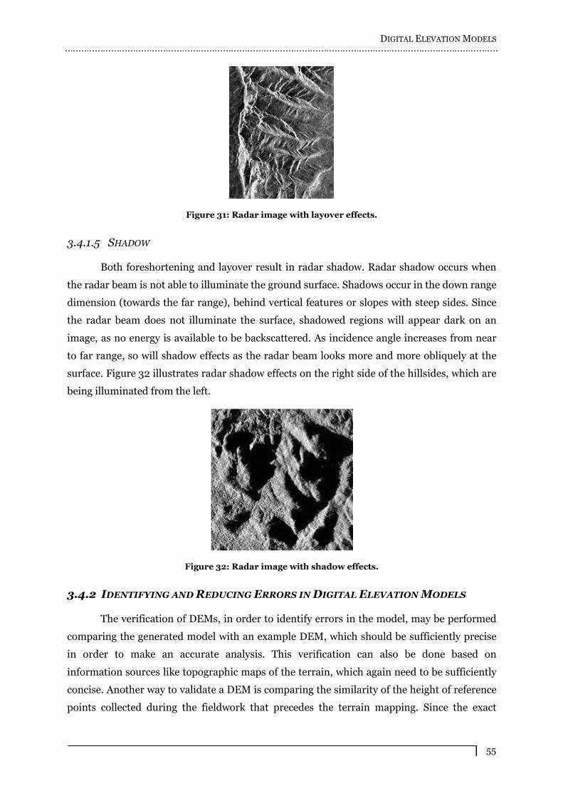
DIGITAL ELEVATION MODELS
55
Figure 31: Radar image with layover effects.
3.4.1.5 SHADOW
Both foreshortening and layover result in radar shadow. Radar shadow occurs when
the radar beam is not able to illuminate the ground surface. Shadows occur in the down range
dimension (towards the far range), behind vertical features or slopes with steep sides. Since
the radar beam does not illuminate the surface, shadowed regions will appear dark on an
image, as no energy is available to be backscattered. As incidence angle increases from near
to far range, so will shadow effects as the radar beam looks more and more obliquely at the
surface. Figure 32 illustrates radar shadow effects on the right side of the hillsides, which are
being illuminated from the left.
Figure 32: Radar image with shadow effects.
3.4.2 IDENTIFYING AND REDUCING ERRORS IN DIGITAL ELEVATION MODELS
The verification of DEMs, in order to identify errors in the model, may be performed
comparing the generated model with an example DEM, which should be sufficiently precise
in order to make an accurate analysis. This verification can also be done based on
information sources like topographic maps of the terrain, which again need to be sufficiently
concise. Another way to validate a DEM is comparing the similarity of the height of reference
points collected during the fieldwork that precedes the terrain mapping. Since the exact

DIGITAL ELEVATION MODELS
56
position and height of these reference points collected manually is known, it is possible to
verify the height of these same positions in the DEM and observe precisely their accuracy. In
this case, it is very important that the reference points are collected from open areas in the
terrain, far from reflective objects such as fences, metallic devices, trees and so on, which can
provoke distortions on the signal backscattered to the radar and, as consequence, produce
the generation of wrong height values at these locations.
Systematic errors are not easily detectable and can introduce significant bias. Many
studies have investigated methods to identify systematic errors in DEMs. Brown and
Bara [BROWN & BARA, 1994 in WECHSLER, 2000] used semi-variograms and fractal
dimensions to confirm the presence and structure of systematic errors in DEMs and
suggested filtering as a means to reduce the error. Theobald [THEOBALD, 1989
in WECHSLER, 2000] reviewed the sources of DEMs and DEM data structure to identify
how bias and errors are produced in DEM generation.
Polidori et al. [POLIDORI ET AL., 1991 in WECHSLER, 2000] used fractal techniques to
identify interpolation artifacts in DEMs. The authors suggest that the fractal dimension could
be used as a DEM quality indicator by revealing directional tendency or excessive smoothing
in the model.
Monckton [MONCKTON, 1994 in WECHSLER, 2000] examined the spatial structure
of errors in a DEM by using the spot height data provided on paper maps. Two methods of
utilizing these spot heights to assess DEMs were employed. The first approach compared the
value of the spot height with the value of the elevation that occurred on the DEM at that exact
location. The second method interpolated the value to be compared with the spot height from
a 55 window surrounding the location where the spot height fell on the DEM. This
experiment justified the use of spot height data in evaluating DEMs, provided by the United
Kingdom�s Ordnance Survey.
Spatial autocorrelation of error was investigated using a variation of Moran�s I
statistic where the weight factor applied was based on the lag distance between points. A
resulting correlogram (weight exponent versus Moran�s I statistic) indicated no spatial
autocorrelation at distances of 250 m.
López [LÓPEZ, 1997] developed a work that attempted to locate some types of
randomly distributed, weakly spatially correlated errors by applying a new methodology
based on Principal Components Analysis. López conducted a prototype implementation using
MATLAB [MATHWORKS, 2004], and the overall procedure has been numerically tested
using a Monte Carlo approach. The preliminary results for the so-called pyramid-like error
shape model were slightly worse than for the spike shaped errors model. The spike-like error
shape model represents completely isolated errors (spatially uncorrelated), and the pyramid-
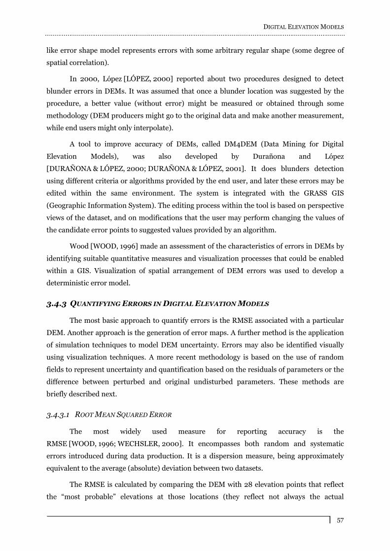
DIGITAL ELEVATION MODELS
57
like error shape model represents errors with some arbitrary regular shape (some degree of
spatial correlation).
In 2000, López [LÓPEZ, 2000] reported about two procedures designed to detect
blunder errors in DEMs. It was assumed that once a blunder location was suggested by the
procedure, a better value (without error) might be measured or obtained through some
methodology (DEM producers might go to the original data and make another measurement,
while end users might only interpolate).
A tool to improve accuracy of DEMs, called DM4DEM (Data Mining for Digital
Elevation Models), was also developed by Durañona and López
[DURAÑONA & LÓPEZ, 2000; DURAÑONA & LÓPEZ, 2001]. It does blunders detection
using different criteria or algorithms provided by the end user, and later these errors may be
edited within the same environment. The system is integrated with the GRASS GIS
(Geographic Information System). The editing process within the tool is based on perspective
views of the dataset, and on modifications that the user may perform changing the values of
the candidate error points to suggested values provided by an algorithm.
Wood [WOOD, 1996] made an assessment of the characteristics of errors in DEMs by
identifying suitable quantitative measures and visualization processes that could be enabled
within a GIS. Visualization of spatial arrangement of DEM errors was used to develop a
deterministic error model.
3.4.3 QUANTIFYING ERRORS IN DIGITAL ELEVATION MODELS
The most basic approach to quantify errors is the RMSE associated with a particular
DEM. Another approach is the generation of error maps. A further method is the application
of simulation techniques to model DEM uncertainty. Errors may also be identified visually
using visualization techniques. A more recent methodology is based on the use of random
fields to represent uncertainty and quantification based on the residuals of parameters or the
difference between perturbed and original undisturbed parameters. These methods are
briefly described next.
3.4.3.1 ROOT MEAN SQUARED ERROR
The most widely used measure for reporting accuracy is the
RMSE [WOOD, 1996; WECHSLER, 2000]. It encompasses both random and systematic
errors introduced during data production. It is a dispersion measure, being approximately
equivalent to the average (absolute) deviation between two datasets.
The RMSE is calculated by comparing the DEM with 28 elevation points that reflect
the �most probable� elevations at those locations (they reflect not always the actual
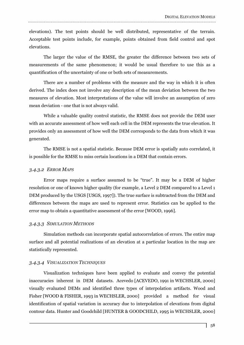
DIGITAL ELEVATION MODELS
58
elevations). The test points should be well distributed, representative of the terrain.
Acceptable test points include, for example, points obtained from field control and spot
elevations.
The larger the value of the RMSE, the greater the difference between two sets of
measurements of the same phenomenon; it would be usual therefore to use this as a
quantification of the uncertainty of one or both sets of measurements.
There are a number of problems with the measure and the way in which it is often
derived. The index does not involve any description of the mean deviation between the two
measures of elevation. Most interpretations of the value will involve an assumption of zero
mean deviation - one that is not always valid.
While a valuable quality control statistic, the RMSE does not provide the DEM user
with an accurate assessment of how well each cell in the DEM represents the true elevation. It
provides only an assessment of how well the DEM corresponds to the data from which it was
generated.
The RMSE is not a spatial statistic. Because DEM error is spatially auto correlated, it
is possible for the RMSE to miss certain locations in a DEM that contain errors.
3.4.3.2 ERROR MAPS
Error maps require a surface assumed to be �true�. It may be a DEM of higher
resolution or one of known higher quality (for example, a Level 2 DEM compared to a Level 1
DEM produced by the USGS [USGS, 1997]). The true surface is subtracted from the DEM and
differences between the maps are used to represent error. Statistics can be applied to the
error map to obtain a quantitative assessment of the error [WOOD, 1996].
3.4.3.3 SIMULATION METHODS
Simulation methods can incorporate spatial autocorrelation of errors. The entire map
surface and all potential realizations of an elevation at a particular location in the map are
statistically represented.
3.4.3.4 VISUALIZATION TECHNIQUES
Visualization techniques have been applied to evaluate and convey the potential
inaccuracies inherent in DEM datasets. Acevedo [ACEVEDO, 1991 in WECHSLER, 2000]
visually evaluated DEMs and identified three types of interpolation artifacts. Wood and
Fisher [WOOD & FISHER, 1993 in WECHSLER, 2000] provided a method for visual
identification of spatial variation in accuracy due to interpolation of elevations from digital
contour data. Hunter and Goodchild [HUNTER & GOODCHILD, 1995 in WECHSLER, 2000]

DIGITAL ELEVATION MODELS
59
identified the errors associated with defining the horizontal position of a terrain elevation
and recommended that users should combine the RMSE statistic with simple probability
theory to communicate uncertainty to the end user. Wood [WOOD, 1996] used the visual
spatial arrangement of DEM error to develop a deterministic error model. A fractal surface
was generated to represent elevation and considered the control elevation surface. Sparse
contours were fit to the surface. Uncertainty associated with four different interpolation
methods was evaluated. Different visualization tools were used to show the differences in the
interpolation methods.
Spear et al. [SPEAR ET AL., 1996 in WECHSLER, 2000] conducted a survey to
investigate the effectiveness of different visualization techniques in conveying interpolation
uncertainty. The authors compared the effectiveness of three visualization representations:
(1) presentation of a map of the interpolated prediction next to a map of the predicted error;
(2) presentation of a confidence interval as three separate maps; (3) presentation of a
confidence interval as one combined map. Participants preferred the three confidence
interval maps closely followed by preference for the combined map.
Visualization of different potential DEM realizations enables users to understand the
potential accuracy loss resulting from DEM creation. However a series of maps identifying
these possible scenarios can overwhelm a decision-maker. Therefore visualization of
uncertainty alone may not be an efficient method for communicating uncertainty to the
decision-maker. Quantitative estimates of error and their consequences should be developed
and provided [ENGLUND, 1993 in WECHSLER, 2000].
Animation has been employed to combine output from the many realizations
produced in Monte Carlo simulations [RUBINSTEIN, 1981] of uncertainty. Movies
containing series of animations can be used to demonstrate the effect of spatial
autocorrelation [EHLSCHLAEGER, 1998] or the effect of adding random error to a DEM.
3.4.3.5 RANDOM FIELDS
Wechsler [WECHSLER, 2000] developed a methodology to quantify uncertainty in
DEMs and in derived parameters, such as slope, upslope area, and topographic index. This
methodology was based on the representation of uncertainty due to random errors in the
form of random fields, and the quantification of the effects of this uncertainty on the DEM
based on the residuals of the parameters. The methodology was implemented within the
ESRI ArcView Spatial Analyst GIS [ESRI, 1998] environment and utilizes Monte Carlo
simulations to quantify DEM uncertainty using random error fields.
Different methods for simulating random error were developed. The methodology and
resulting tool were applied to investigate the effects of uncertainty on elevation and derived

DIGITAL ELEVATION MODELS
60
topographic parameters, the effects of uncertainty on DEMs of different scale, and the effects
of uncertainty in flat and varied terrain. Results demonstrated that DEM parameters were
affected by random errors, and this effect varied with the method in which the random error
was represented. DEM error manifested itself differently in DEMs of diverse scales. At higher
grid resolution, slope and topographic index were more susceptible to DEM error than
elevation and upslope area. Slope and upslope area grids were more sensitive to uncertainty
than elevation and topographic index grids with a more pronounced effect in flatter areas.
3.5 FINAL REMARKS
DEMs may contain several errors, what causes uncertainty about the reliability of the
data. The detection of these errors is highly desirable, because errors significantly affect all
statistics habitually used to report about the quality of the generated model. Performing a
quality control of the model by comparing height values of specific coordinates with their
corresponding values in the real surface may help remote sensing users to detect most of
these errors. However, a critical problem is the fact that these errors can be caused by many
different reasons for each generated DEM, what makes their identification and correction
very difficult.
Although several studies have proposed methodologies to detect and quantify, and
also to remove different kinds of errors, these procedures cannot guarantee that the DEM is
precise. This happens because the applied algorithms are specialized in detecting errors with
particular characteristics, producing good results only when the model contains
predominantly these special types of errors. This can be observed in Table 1, which presents a
brief synthesis of the main identification, quantification and removal methods, described in
this chapter, where the type of error or error characteristic they approach can be visualized.
During the development of this thesis, and interacting strongly with (In)SAR data
users, it could be observed that the knowledge that these experienced users own can be
efficiently and intuitively used to identify and remove errors in DEMs. Traditionally,
experienced SAR data users employ their previous acquired knowledge about the data
combined with some powerful analysis tools to make final adjustments to the DEMs and,
therefore, build more precise models. Although, this becomes an arduous, time demanding
and inefficient task since there do not exist specialized tools to perform the corrections. This
fact can also be observed in Table 1, since only one removal tool (the DM4DEM prototype)
could be listed in the presented synthesis.
The association of these analysis tools and sophisticated editing methods with 3D
interfaces, that provide realistic and interactive data visualization and exploration, will allow
expert DEM users to perform identification and correction of errors (of different types) in an
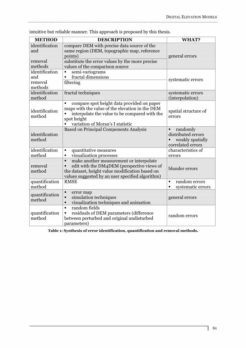
DIGITAL ELEVATION MODELS
61
intuitive but reliable manner. This approach is proposed by this thesis.
METHOD DESCRIPTION WHAT?
compare DEM with precise data source of the
same region (DEM, topographic map, reference
points)
identification
and
removal
methods substitute the error values by the more precise
values of the comparison source
general errors
semi-variograms
fractal dimensions
identification
and
removal
methods filtering
systematic errors
identification
method
fractal techniques systematic errors
(interpolation)
identification
method
compare spot height data provided on paper
maps with the value of the elevation in the DEM
interpolate the value to be compared with the
spot height
variation of Moran�s I statistic
spatial structure of
errors
identification
method
Based on Principal Components Analysis randomly
distributed errors
weakly spatially
correlated errors
identification
method
quantitative measures
visualization processes
characteristics of
errors
removal
method
make another measurement or interpolate
edit with the DM4DEM (perspective views of
the dataset, height value modification based on
values suggested by an user specified algorithm)
blunder errors
quantification
method
RMSE random errors
systematic errors
quantification
method
error map
simulation techniques
visualization techniques and animation
general errors
quantification
method
random fields
residuals of DEM parameters (difference
between perturbed and original undisturbed
parameters)
random errors
Table 1: Synthesis of error identification, quantification and removal methods.
CHAPTER 4
VISUALIZATION, INTERACTION AND EDITING
4.1 INTRODUCTION TO THE CHAPTER
The remote sensing community normally visualizes and manipulates its data using 2D
interface based systems. These systems are very well accepted by the users and offer
sophisticated functions for, mainly, analyze the data. However, remote sensing data, such as
DEMs, have a 3D nature because they represent Earth�s surface. Shape, height and depth are
inherent features of these data that cannot be intuitively and realistically represented with 2D
interfaces, making the realization of processing and quality control tasks, as well as editing
procedures, arduous.
VR uses three dimensions to represent and present data, and to interact with data in
order to retrieve the information they contain. High-resolution, realistic virtual environments
can actually be constructed, also with desktop VR technology.
This chapter shows how DEMs can be visualized and manipulated using 2D and 3D
interfaces. Only non-immersive VR interfaces are considered here, since the immersive
approach needs special devices and platforms, what is not the case for this thesis. The
techniques explained in the text fulfill the requirements of the methodology proposed by this
thesis, and therefore of the system that validates this methodology.
Editing methods are also briefly described in this chapter, in order to construct a
background about some techniques that can be effectively used to edit terrain surfaces, such
as selection methods, cut and paste tools, among others.
4.2 VISUALIZING DIGITAL ELEVATION MODELS
Visualization technology is indeed very useful, enabling users to understand masses of
data. Visualization systems may be categorized in two main classes: the ones that use 2D
interfaces, and the ones that exploit the 3D paradigm. This classification is related to the way
the data to be visualized are represented.
4.2.1 TWO-DIMENSIONAL INTERFACES
DEMs are traditionally visualized and analyzed through 2D interfaces. There are
several classical manners of visualizing and assessing DEMs: contour lines or levels, gray
levels, perspective views and compound plots. These are presented in the following, being the
transcription of the text extracted, partially, from the paper titled �Simulation and
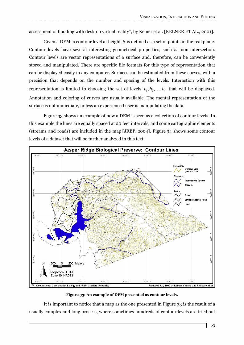
VISUALIZATION, INTERACTION AND EDITING
63
assessment of flooding with desktop virtual reality�, by Kelner et al. [KELNER ET AL., 2001].
Given a DEM, a contour level at height h is defined as a set of points in the real plane.
Contour levels have several interesting geometrical properties, such as non-intersection.
Contour levels are vector representations of a surface and, therefore, can be conveniently
stored and manipulated. There are specific file formats for this type of representation that
can be displayed easily in any computer. Surfaces can be estimated from these curves, with a
precision that depends on the number and spacing of the levels. Interaction with this
representation is limited to choosing the set of levels
hhh ,,, 21 that will be displayed.
Annotation and coloring of curves are usually available. The mental representation of the
surface is not immediate, unless an experienced user is manipulating the data.
Figure 33 shows an example of how a DEM is seen as a collection of contour levels. In
this example the lines are equally spaced at 20 feet intervals, and some cartographic elements
(streams and roads) are included in the map [JRBP, 2004]. Figure 34 shows some contour
levels of a dataset that will be further analyzed in this text.
Figure 33: An example of DEM presented as contour levels.
It is important to notice that a map as the one presented in Figure 33 is the result of a
usually complex and long process, where sometimes hundreds of contour levels are tried out
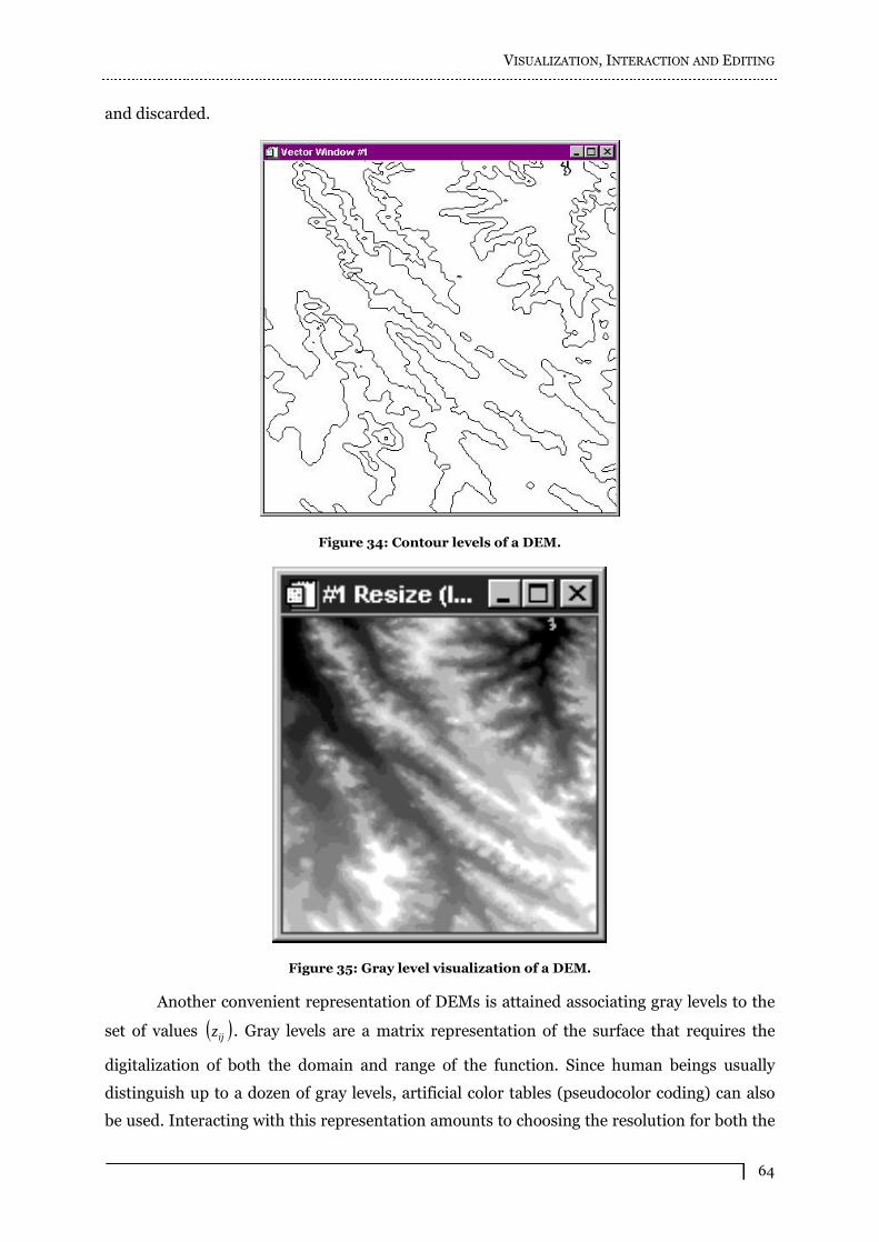
VISUALIZATION, INTERACTION AND EDITING
64
and discarded.
Figure 34: Contour levels of a DEM.
Figure 35: Gray level visualization of a DEM.
Another convenient representation of DEMs is attained associating gray levels to the
set of values ijz . Gray levels are a matrix representation of the surface that requires the
digitalization of both the domain and range of the function. Since human beings usually
distinguish up to a dozen of gray levels, artificial color tables (pseudocolor coding) can also
be used. Interacting with this representation amounts to choosing the resolution for both the

VISUALIZATION, INTERACTION AND EDITING
65
grid (matrix size) and the levels (pixel depth), and eventually specifying the color table. A
mental model may be easier to grasp than with the previous representation, but at the cost of
losing precision.
For instance, drawing as black the minimum height, as white the maximum and as
intermediate gray levels values in between, an image-like representation is obtained.
Figure 35 illustrates this method using the dataset presented in Figure 34.
Direct visualization of data can also be used. A perspective view is always interesting,
because it is intuitive. In order to do this, standard software with graphical abilities can be
used. The problem with this kind of information representation is that it may be hard to have
the complete scene with a single perspective view. Many views could be generated to improve
this situation, but with dubious results. Figure 36 shows the perspective visualization of the
same dataset presented in Figure 34 and in Figure 35.
Figure 36: Perspective visualization of a DEM.
Compound visualization, where contour levels, gray levels and a perspective view are
overlaid, is the richest of all the possibilities. It can be built using some advanced platforms
such as IDL (Interactive Data Language) [IDL, 1998] or ENVI (ENvironment for Visualizing
Images) [RESEARCH SYSTEMS, 2004]. It is computer demanding and, for this reason, no
system offers tools for simultaneously rendering, navigating and editing such a structure.
Figure 37 illustrates a compound view of a DEM, with gray levels at the bottom,
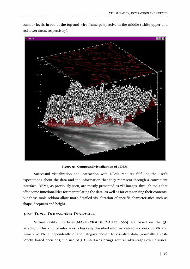
VISUALIZATION, INTERACTION AND EDITING
66
contour levels in red at the top and wire frame perspective in the middle (white upper and
red lower faces, respectively).
Figure 37: Compound visualization of a DEM.
Successful visualization and interaction with DEMs requires fulfilling the user�s
expectations about the data and the information that they represent through a convenient
interface. DEMs, as previously seen, are mostly presented as 2D images, through tools that
offer some functionalities for manipulating the data, as well as for categorizing their contents,
but these tools seldom allow more detailed visualization of specific characteristics such as
shape, deepness and height.
4.2.2 THREE-DIMENSIONAL INTERFACES
Virtual reality interfaces [MAZURYK & GERVAUTZ, 1996] are based on the 3D
paradigm. This kind of interfaces is basically classified into two categories: desktop VR and
immersive VR. Independently of the category chosen to visualize data (normally a cost-
benefit based decision), the use of 3D interfaces brings several advantages over classical
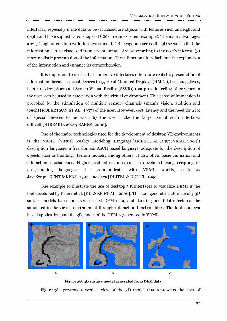
VISUALIZATION, INTERACTION AND EDITING
67
interfaces, especially if the data to be visualized are objects with features such as height and
depth and have sophisticated shapes (DEMs are an excellent example). The main advantages
are: (1) high interaction with the environment; (2) navigation across the 3D scene, so that the
information can be visualized from several points of view according to the user�s interest; (3)
more realistic presentation of the information. These functionalities facilitate the exploration
of the information and enhance its comprehension.
It is important to notice that immersive interfaces offer more realistic presentation of
information, because special devices (e.g., Head Mounted Displays (HMDs), trackers, gloves,
haptic devices, Surround Screen Virtual Reality (SSVR)) that provide feeling of presence to
the user, can be used in association with the virtual environment. This sense of immersion is
provoked by the stimulation of multiple sensory channels (mainly vision, audition and
touch) [ROBERTSON ET AL., 1997] of the user. However, cost, latency and the need for a lot
of special devices to be worn by the user make the large use of such interfaces
difficult [HIBBARD, 2000; BAKER, 2000].
One of the major technologies used for the development of desktop VR environments
is the VRML (Virtual Reality Modeling Language [AMES ET AL., 1997; VRML, 2004])
description language, a free domain ASCII based language, adequate for the description of
objects such as buildings, terrain models, among others. It also offers basic animation and
interaction mechanisms. Higher-level interactions can be developed using scripting or
programming languages that communicate with VRML worlds, such as
JavaScript [KENT & KENT, 1997] and Java [DEITEL & DEITEL, 1998].
One example to illustrate the use of desktop VR interfaces to visualize DEMs is the
tool developed by Kelner et al. [KELNER ET AL., 2000]. This tool generates automatically 3D
surface models based on user selected DEM data, and flooding and tidal effects can be
simulated in the virtual environment through interaction functionalities. The tool is a Java
based application, and the 3D model of the DEM is generated in VRML.
a
b
c
Figure 38: 3D surface model generated from DEM data.
Figure 38a presents a vertical view of the 3D model that represents the area of
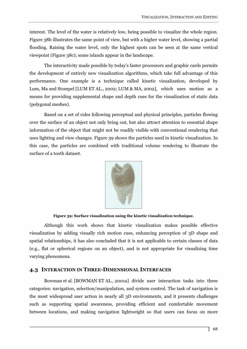
VISUALIZATION, INTERACTION AND EDITING
68
interest. The level of the water is relatively low, being possible to visualize the whole region.
Figure 38b illustrates the same point of view, but with a higher water level, showing a partial
flooding. Raising the water level, only the highest spots can be seen at the same vertical
viewpoint (Figure 38c); some islands appear in the landscape.
The interactivity made possible by today�s faster processors and graphic cards permits
the development of entirely new visualization algorithms, which take full advantage of this
performance. One example is a technique called kinetic visualization, developed by
Lum, Ma and Stompel [LUM ET AL., 2002; LUM & MA, 2002], which uses motion as a
means for providing supplemental shape and depth cues for the visualization of static data
(polygonal meshes).
Based on a set of rules following perceptual and physical principles, particles flowing
over the surface of an object not only bring out, but also attract attention to essential shape
information of the object that might not be readily visible with conventional rendering that
uses lighting and view changes. Figure 39 shows the particles used in kinetic visualization. In
this case, the particles are combined with traditional volume rendering to illustrate the
surface of a tooth dataset.
Figure 39: Surface visualization using the kinetic visualization technique.
Although this work shows that kinetic visualization makes possible effective
visualization by adding visually rich motion cues, enhancing perception of 3D shape and
spatial relationships, it has also concluded that it is not applicable to certain classes of data
(e.g., flat or spherical regions on an object), and is not appropriate for visualizing time
varying phenomena.
4.3 INTERACTION IN THREE-DIMENSIONAL INTERFACES
Bowman et al. [BOWMAN ET AL., 2001a] divide user interaction tasks into three
categories: navigation, selection/manipulation, and system control. The task of navigation is
the most widespread user action in nearly all 3D environments, and it presents challenges
such as supporting spatial awareness, providing efficient and comfortable movement
between locations, and making navigation lightweight so that users can focus on more
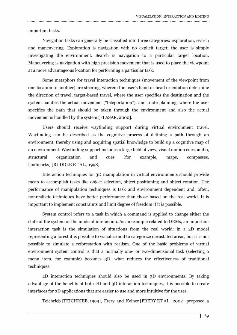
VISUALIZATION, INTERACTION AND EDITING
69
important tasks.
Navigation tasks can generally be classified into three categories: exploration, search
and maneuvering. Exploration is navigation with no explicit target; the user is simply
investigating the environment. Search is navigation to a particular target location.
Maneuvering is navigation with high precision movement that is used to place the viewpoint
at a more advantageous location for performing a particular task.
Some metaphors for travel interaction techniques (movement of the viewpoint from
one location to another) are steering, wherein the user�s hand or head orientation determine
the direction of travel, target-based travel, where the user specifies the destination and the
system handles the actual movement (�teleportation�), and route planning, where the user
specifies the path that should be taken through the environment and also the actual
movement is handled by the system [FLASAR, 2000].
Users should receive wayfinding support during virtual environment travel.
Wayfinding can be described as the cognitive process of defining a path through an
environment, thereby using and acquiring spatial knowledge to build up a cognitive map of
an environment. Wayfinding support includes a large field of view, visual motion cues, audio,
structural organization and cues (for example, maps, compasses,
landmarks) [RUDDLE ET AL., 1998].
Interaction techniques for 3D manipulation in virtual environments should provide
mean to accomplish tasks like object selection, object positioning and object rotation. The
performance of manipulation techniques is task and environment dependent and, often,
nonrealistic techniques have better performance than those based on the real world. It is
important to implement constraints and limit degree of freedom if it is possible.
System control refers to a task in which a command is applied to change either the
state of the system or the mode of interaction. As an example related to DEMs, an important
interaction task is the simulation of situations from the real world: in a 2D model
representing a forest it is possible to visualize and to categorize devastated areas, but it is not
possible to simulate a reforestation with realism. One of the basic problems of virtual
environment system control is that a normally one- or two-dimensional task (selecting a
menu item, for example) becomes 3D, what reduces the effectiveness of traditional
techniques.
2D interaction techniques should also be used in 3D environments. By taking
advantage of the benefits of both 2D and 3D interaction techniques, it is possible to create
interfaces for 3D applications that are easier to use and more intuitive for the user.
Teichrieb [TEICHRIEB, 1999], Frery and Kelner [FRERY ET AL., 2002] proposed a
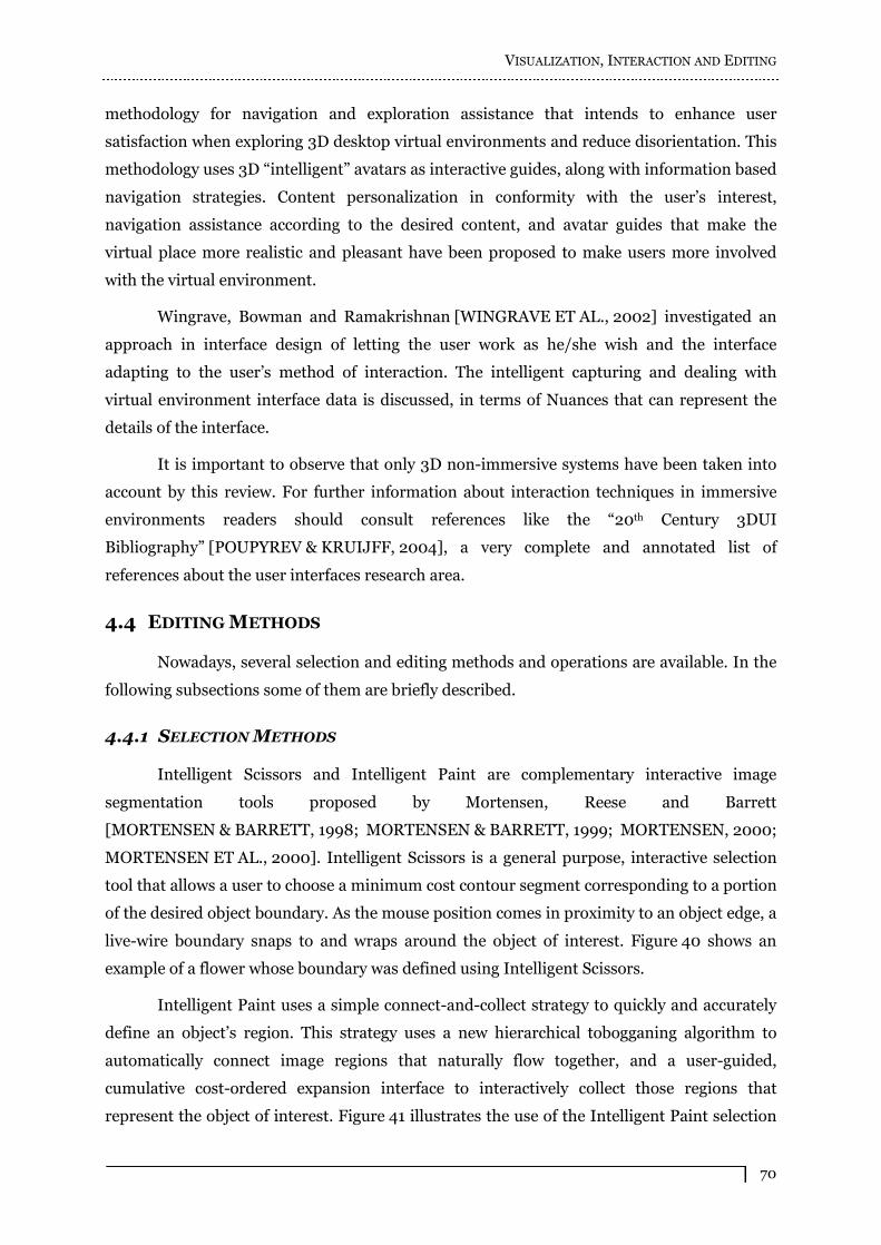
VISUALIZATION, INTERACTION AND EDITING
70
methodology for navigation and exploration assistance that intends to enhance user
satisfaction when exploring 3D desktop virtual environments and reduce disorientation. This
methodology uses 3D �intelligent� avatars as interactive guides, along with information based
navigation strategies. Content personalization in conformity with the user�s interest,
navigation assistance according to the desired content, and avatar guides that make the
virtual place more realistic and pleasant have been proposed to make users more involved
with the virtual environment.
Wingrave, Bowman and Ramakrishnan [WINGRAVE ET AL., 2002] investigated an
approach in interface design of letting the user work as he/she wish and the interface
adapting to the user�s method of interaction. The intelligent capturing and dealing with
virtual environment interface data is discussed, in terms of Nuances that can represent the
details of the interface.
It is important to observe that only 3D non-immersive systems have been taken into
account by this review. For further information about interaction techniques in immersive
environments readers should consult references like the �20th Century 3DUI
Bibliography� [POUPYREV & KRUIJFF, 2004], a very complete and annotated list of
references about the user interfaces research area.
4.4 EDITING METHODS
Nowadays, several selection and editing methods and operations are available. In the
following subsections some of them are briefly described.
4.4.1 SELECTION METHODS
Intelligent Scissors and Intelligent Paint are complementary interactive image
segmentation tools proposed by Mortensen, Reese and Barrett
[MORTENSEN & BARRETT, 1998; MORTENSEN & BARRETT, 1999; MORTENSEN, 2000;
MORTENSEN ET AL., 2000]. Intelligent Scissors is a general purpose, interactive selection
tool that allows a user to choose a minimum cost contour segment corresponding to a portion
of the desired object boundary. As the mouse position comes in proximity to an object edge, a
live-wire boundary snaps to and wraps around the object of interest. Figure 40 shows an
example of a flower whose boundary was defined using Intelligent Scissors.
Intelligent Paint uses a simple connect-and-collect strategy to quickly and accurately
define an object�s region. This strategy uses a new hierarchical tobogganing algorithm to
automatically connect image regions that naturally flow together, and a user-guided,
cumulative cost-ordered expansion interface to interactively collect those regions that
represent the object of interest. Figure 41 illustrates the use of the Intelligent Paint selection

VISUALIZATION, INTERACTION AND EDITING
71
tool. Figure 41b presents the defined region showing the mouse movements (white lines) and
mouse clicks (mouse pressing: green circle; mouse releasing: red circle).
Figure 40: Boundary definition with Intelligent Scissors.
a
b
Figure 41: Selection: a) image of a bird; b) region definition with Intelligent Paint.
4.4.2 EDITING METHODS
Next, a cut and paste editing method for multiresolution surfaces, a point-based
surface editing method, and some image editing methods are presented. These editing
methods give a brief overview of techniques nowadays in use.
4.4.2.1 CUT AND PASTE EDITING OF MULTIRESOLUTION SURFACES
Cut and paste operations to combine different elements into a common structure are
widely used operations that have been successfully adapted to many media types. Biermann

VISUALIZATION, INTERACTION AND EDITING
72
and co-workers [BIERMANN ET AL., 2002] describe a set of algorithms based on
multiresolution subdivision surfaces that perform at interactive rates and enable intuitive cut
and paste operations. In order to perform pasting the user selects an area of interest on the
source surface. Both the source and the target surfaces are separated into base and detail,
such that the detail surface represents a vector offset over the base surface. Next, the user
specifies a location and an orientation on the target surface where the source feature is to be
pasted and interactively adjusts the position, orientation, and size of the pasted feature.
Figure 42 illustrates (row-wise from top left) the main steps needed to perform the
pasting operating: a) feature selection on the source surface; b) base source surface; c) source
parameterization onto the plane; d) target region finding by geodesic walking; e) source
(black) and target (red) parameterizations superimposed in the plane; f) source feature
pasted onto the target surface.
Figure 42: Cut and paste algorithm for editing of multiresolution surfaces.
4.4.2.2 POINT-BASED SURFACE EDITING
Figure 43: Editing of a point-sampled object: carving.
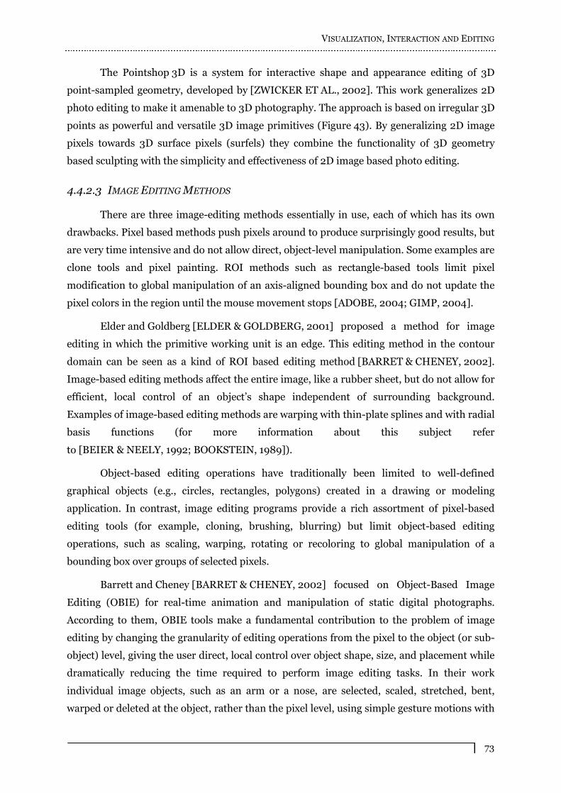
VISUALIZATION, INTERACTION AND EDITING
73
The Pointshop 3D is a system for interactive shape and appearance editing of 3D
point-sampled geometry, developed by [ZWICKER ET AL., 2002]. This work generalizes 2D
photo editing to make it amenable to 3D photography. The approach is based on irregular 3D
points as powerful and versatile 3D image primitives (Figure 43). By generalizing 2D image
pixels towards 3D surface pixels (surfels) they combine the functionality of 3D geometry
based sculpting with the simplicity and effectiveness of 2D image based photo editing.
4.4.2.3 IMAGE EDITING METHODS
There are three image-editing methods essentially in use, each of which has its own
drawbacks. Pixel based methods push pixels around to produce surprisingly good results, but
are very time intensive and do not allow direct, object-level manipulation. Some examples are
clone tools and pixel painting. ROI methods such as rectangle-based tools limit pixel
modification to global manipulation of an axis-aligned bounding box and do not update the
pixel colors in the region until the mouse movement stops [ADOBE, 2004; GIMP, 2004].
Elder and Goldberg [ELDER & GOLDBERG, 2001] proposed a method for image
editing in which the primitive working unit is an edge. This editing method in the contour
domain can be seen as a kind of ROI based editing method [BARRET & CHENEY, 2002].
Image-based editing methods affect the entire image, like a rubber sheet, but do not allow for
efficient, local control of an object�s shape independent of surrounding background.
Examples of image-based editing methods are warping with thin-plate splines and with radial
basis functions (for more information about this subject refer
to [BEIER & NEELY, 1992; BOOKSTEIN, 1989]).
Object-based editing operations have traditionally been limited to well-defined
graphical objects (e.g., circles, rectangles, polygons) created in a drawing or modeling
application. In contrast, image editing programs provide a rich assortment of pixel-based
editing tools (for example, cloning, brushing, blurring) but limit object-based editing
operations, such as scaling, warping, rotating or recoloring to global manipulation of a
bounding box over groups of selected pixels.
Barrett and Cheney [BARRET & CHENEY, 2002] focused on Object-Based Image
Editing (OBIE) for real-time animation and manipulation of static digital photographs.
According to them, OBIE tools make a fundamental contribution to the problem of image
editing by changing the granularity of editing operations from the pixel to the object (or sub-
object) level, giving the user direct, local control over object shape, size, and placement while
dramatically reducing the time required to perform image editing tasks. In their work
individual image objects, such as an arm or a nose, are selected, scaled, stretched, bent,
warped or deleted at the object, rather than the pixel level, using simple gesture motions with
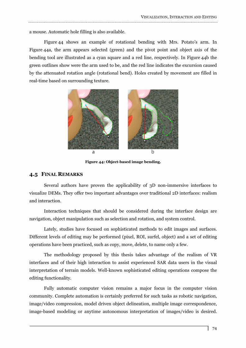
VISUALIZATION, INTERACTION AND EDITING
74
a mouse. Automatic hole filling is also available.
Figure 44 shows an example of rotational bending with Mrs. Potato�s arm. In
Figure 44a, the arm appears selected (green) and the pivot point and object axis of the
bending tool are illustrated as a cyan square and a red line, respectively. In Figure 44b the
green outlines show were the arm used to be, and the red line indicates the excursion caused
by the attenuated rotation angle (rotational bend). Holes created by movement are filled in
real-time based on surrounding texture.
Figure 44: Object-based image bending.
4.5 FINAL REMARKS
Several authors have proven the applicability of 3D non-immersive interfaces to
visualize DEMs. They offer two important advantages over traditional 2D interfaces: realism
and interaction.
Interaction techniques that should be considered during the interface design are
navigation, object manipulation such as selection and rotation, and system control.
Lately, studies have focused on sophisticated methods to edit images and surfaces.
Different levels of editing may be performed (pixel, ROI, surfel, object) and a set of editing
operations have been practiced, such as copy, move, delete, to name only a few.
The methodology proposed by this thesis takes advantage of the realism of VR
interfaces and of their high interaction to assist experienced SAR data users in the visual
interpretation of terrain models. Well-known sophisticated editing operations compose the
editing functionality.
Fully automatic computer vision remains a major focus in the computer vision
community. Complete automation is certainly preferred for such tasks as robotic navigation,
image/video compression, model driven object delineation, multiple image correspondence,
image-based modeling or anytime autonomous interpretation of images/video is desired.

VISUALIZATION, INTERACTION AND EDITING
75
However, general purpose image editing will continue to require human guidance due to the
essential role of the user in the creative process and in identifying the image components of
interest.

CHAPTER 5
VIRTUAL REALITY INTERFACES APPLIED TO ENHANCE
DIGITAL ELEVATION MODELS
5.1 INTRODUCTION TO THE CHAPTER
This thesis proposes a methodology based on VR interfaces aiming to resolve the
problem of correcting elevation errors in DEMs, in order to enhance them. In this chapter,
the tackled problem is explained, so that the main difficulties can be understood, and in
sequence the methodology is described.
Two facts make up the motivation for this thesis: (1) DEMs present elevation errors
produced by different kinds of problems, which should be corrected in an intuitive and
efficient way relieving the need for specific detection and removing algorithms that specialize
in finding errors with particular characteristics, and (2) the remote sensing community, as far
as it is known, has not got an efficient and complete tool for this purpose. Such a tool should
combine a realistic visualization and intuitive manipulation of the data, as well as a
qualitative analysis, together with a toolkit composed of editing functionalities for correction
of different types of errors found in a DEM.
According to the methodology, expert remote sensing data users have to perform
three basic activities in a virtual environment presenting a 3D DEM, for the purpose of
identifying and removing errors. One of these three activities comprises DEM visualization
and exploration, in order to obtain knowledge about the data that can be used to make a
visual interpretation and verification of the model. Analyze the DEM using specialized
analysis tools, so that statistical features and representations can be used to identify error
areas in the model, is another activity to be performed by the user. Finally, a third activity is
the editing of error areas found in the dataset, in order to enhance the DEM.
Considerations about differences between the proposed methodology and other
methods mentioned in the literature are also presented at the end of the chapter,
demonstrating why the VR based approach of this thesis is successful and more effective in
the identification and correction of errors in DEMs.
5.2 PROBLEM STATEMENT
DEMs contain inherently elevation errors, due to the imaging process used to collect
raw data and their processing to generate products (e.g., cartographic maps, ortho images,
DEMs) [USGS, 1997; WECHSLER, 2000]. The complexity of the imaged relief may also
VIRTUAL REALITY INTERFACES APPLIED TO ENHANCE DIGITAL ELEVATION MODELS
77
cause severe geometric distortions on the final elevation model. Therefore, these models can
have different types of errors, originated by different causes. For example, blunders
associated with the data collection process, systematic errors introduced by systems and/or
procedures used in the data collection and DEM generation processes, and random errors
resulting from accidental and unknown combinations of causes (see
subsection Errors in Digital Elevation Models).
DEMs, after their generation, are submitted to a quality control, in order to verify if
the required precision has been accomplished. This quality level is a relevant point to be
considered, since remote sensing companies have to agree with rigorous precision levels in
order to sale their products. Besides, DEMs, in order to be conveniently used, should be a
reliable information source about the region they represent. Actually, expert remote sensing
data users perform this task manipulating DEMs with 2D systems combined with proper
analysis tools, such as IDL and ENVI. The knowledge about the data owned by the users is
decisive to make successful decisions about which adjustments should be performed on the
DEMs. When needed, users correct data realizing arduous and time demanding editing tasks
using command line based interfaces.
Summarizing, two facts make up the motivation for this research work: (1) DEMs
present elevation errors produced by different kinds of problems, which should be corrected
in an intuitive and efficient way relieving the need for specific detection and removing
algorithms that specialize in detecting errors with particular characteristics, and (2) the
remote sensing community, as far as it is known, has not got an efficient and complete tool
for this purpose. Such a tool should combine a realistic visualization and intuitive
manipulation of the data, as well as a qualitative analysis, together with a toolkit composed of
editing functionalities for correction of different types of errors found in the DEM.
This thesis is related to the accuracy improvement of DEMs. It will not consider errors
in the generation process of DEMs, but will concentrate on errors remaining in the final
product.
5.3 METHODOLOGY: VIRTUAL REALITY INTERFACES APPLIED TO CORRECT
ELEVATION ERRORS IN DIGITAL ELEVATION MODELS
The approach proposed by this thesis in order to correct elevation errors in DEMs is
based on VR interfaces. These interfaces are used to perform visualization and exploration of
the data, as well as statistical analyses in order to identify errors, and editing of errors found
in the models. Once adjusted, these models become more accurate, as well as reliable.
According to the methodology, expert remote sensing data users have to perform
three basic activities in a virtual environment presenting a 3D DEM:
VIRTUAL REALITY INTERFACES APPLIED TO ENHANCE DIGITAL ELEVATION MODELS
78
visualize the DEM and explore it, in order to obtain knowledge about the data that can be
used to make a visual interpretation and verification of the model;
analyze the DEM using specialized analysis tools, so that precise statistical values can be
used to find error areas;
edit error areas identified visually and/or through statistical analyses, enhancing the
DEM.
It is important to say that users that utilize the methodology should own knowledge
about the data to be corrected (e.g., InSAR data), in order to produce as good as possible
results. This requirement is due to the fact that visual interpretation plays an important role
in this methodology, which exploits user�s knowledge in the decision-making process about
areas in the DEM to be enhanced.
5.3.1 VISUALIZATION OF DIGITAL ELEVATION MODELS
How the user chooses to portray a dataset can have a significant effect on how
accurately and efficiently visualization communicates the information the user seeks to
reveal. Therefore, an assumption that can be made is that when visualization is performed in
three dimensions and in an interactive manner, the user is able to quickly derive expressive
visualizations. Such visualizations may be accomplished using VR technology.
Following the methodology, the major way of representing and visualizing a DEM is
as a 3D surface, constructed based on its corresponding InSAR data. In order to add
emphasis and clarity to aspects of the visualization that are of interest for the user, rendering
parameters may be selected.
The DEM may also be presented using contour levels. A functionality to enhance
visualization in the VR environment is to present data as a compound view, composed by the
3D surface, overlapped by contour levels. This form of visualization is usually used to
enhance comprehension of elevation data in two dimensions, as can be seen in Figure 34,
what is also true in three dimensions.
Color can be manipulated based on height to improve height perception. Often
warmer hues are used for the lower values and become cooler in the higher values. Each
vertex of the surface is mapped with height-based predefined colors, so that terrain�s shape
can be easily observed.
Wrap 3D objects with textures is a sophisticated way to enhance the realism of
content presented in VR. Specialized research groups have given special effort to produce
textures of high-resolution and at the same time usable, so that the objects can be loaded in a
low time consuming manner. In the DEM context, the amplitude image generated from the

VIRTUAL REALITY INTERFACES APPLIED TO ENHANCE DIGITAL ELEVATION MODELS
79
same raw data as the DEM is an adequate texture to be used. The virtual terrain, wrapped
with its corresponding amplitude image, allows the reproduction of the terrain appearance
(vegetation coverage, for example) in the real world, when imaged by the sensor (see
Figure 58 in subsection Digital Elevation Model Representation).
5.3.2 INTERACTION IN THE VIRTUAL ENVIRONMENT
The variety of reported interaction techniques can be overwhelming for the developer.
However, some general principles regarding the choice of these techniques can be stated.
None of the techniques can be identified as the best: their effectiveness is task and
environment dependent. Often, nonrealistic techniques have better performance than those
based on the real world.
Navigation, manipulation and system control are the three types of interaction
activities that normally take place in a virtual environment [BOWMAN ET AL., 2001a;
WINGRAVE ET AL., 2002]. The presented methodology uses techniques that make possible
to the user perform these interaction activities to explore and edit errors on DEMs.
5.3.2.1 TWO-DIMENSIONAL INTERACTION
A common misconception in 3D user interface design is that, because the applications
usually contain 3D worlds in which users can create, select, and manipulate 3D objects, the
interaction design space should utilize only 3D interaction. In reality, 2D interaction offers a
number of distinct advantages (very accurate, picking objects is much easier in two
dimensions) over 3D interaction techniques for certain tasks. If haptic or tactile devices are
not present, 2D interaction on a physical surface provides a sense of feedback that is
especially useful for drawing and annotating. By taking advantage of the benefits of both 2D
and 3D interaction techniques, it can be created interfaces for 3D applications that are easy
to use and intuitive for the user.
The methodology described here intends to apply both, 2D and 3D interaction
techniques. It suggests the use of widget-based interfaces, with menus, sliders, buttons and
command-line input, to perform specific navigation, manipulation and system control tasks.
5.3.2.2 NAVIGATION
The methodology uses different metaphors to travel through the virtual environment
(move the viewpoint of the user from one location to another, considering his/her orientation
as well):
steering: the user specifies continuously the direction of motion, using a pointing
technique. The user�s hand orientation determines the direction of travel, moving forward
VIRTUAL REALITY INTERFACES APPLIED TO ENHANCE DIGITAL ELEVATION MODELS
80
with the mouse;
target-based travel: the user specifies the destination, and the system handles the actual
movement. This may take the form of �teleportation�, in which the user jumps
immediately to the new location, or, preferably, the system may perform some
transitional movement between the starting point and the destination;
route planning: the user specifies the path that should be taken through the environment,
and the system handles the actual movement. These techniques allow the user to control
travel while he/she retains the ability to perform other tasks during motion.
5.3.2.3 OBJECT MANIPULATION
Interaction techniques for 3D manipulation in virtual environments should provide
means to accomplish at least one of three basic tasks: object selection, object positioning, and
object rotation. Direct hand manipulation is a major interaction modality in physical
environments, so that the design of interaction techniques in virtual environments using this
metaphor has a profound effect on the environment user interface.
The methodology uses the approach of �touching� an object with the mouse to select it
and then rotate or translate it. This approach simulates a real-world interaction with objects.
Some objects in the virtual environment, in order to perform predefined actions, are
associated to touch sensors. The user may select them and after that, for example, change
their position in the virtual world or scale them.
5.3.2.4 SYSTEM CONTROL
System control refers to a task in which a command is applied to change either the
system state or the interaction mode. System control is often part of another task, like
manipulation.
The use of tools, that is to say, virtual objects and menu systems with an implicit
function or mode, is a technique used for virtual environments and adopted by this
methodology.
5.3.3 ANALYSIS OF DIGITAL ELEVATION MODELS
Interpretation and analysis of remote sensing imagery involves the identification
and/or measurement of various targets (points, lines, area features) in an image in order to
extract useful information about them. A human interpreter performs much interpretation
and identification of targets in remote sensing imagery manually or visually. Digital
processing and analysis may be used to enhance data as a prelude to visual interpretation.
Digital processing and analysis may also be carried out, in order to automatically identify
VIRTUAL REALITY INTERFACES APPLIED TO ENHANCE DIGITAL ELEVATION MODELS
81
targets and extract information completely without manual intervention by a human
interpreter. However, rarely is digital processing and analysis carried out as a complete
replacement for manual interpretation. Often, it is done to supplement and assist the human
analyst.
Remote sensing data users perform analysis on data using some well-established
methods. The proposed methodology approaches analysis through the use of a histogram
tool, a tool to extract profiles, a position-height pick up tool, as well as through the
verification of statistical information about the DEM, such as mean, variance, skewness and
kurtosis, and the minimum and maximum height values of the dataset. This set of analysis
tools has been defined based on requirements specified by expert DEM users.
5.3.3.1 HISTOGRAM
Contrast enhancement involves changing the original values of an image whose useful
data often populates only a small portion of the available range of digital values (e.g., 256
levels for an 8 bit image), so that more of the available range is used, thereby increasing the
contrast between targets and their backgrounds. By manipulating the range of digital values
in an image, it can be applied assorted enhancements to the data. The key to understand
contrast enhancements is to understand the concept of a histogram.
A histogram of a digital image with gray levels in the interval ]1,0[ L is a discrete
function nnrp kk / , where kr is the thk gray level in the image, kn is the number of pixels
in the image with this gray level, n is the total number of pixels in the image and
1,,2,1,0 Lk . It can be said that krp gives an estimate of the probability to occur the
gray level kr [GONZALEZ & WOODS, 2000].
The histogram is a graphical statistical representation of this function. Each entry on
the horizontal axis of the histogram is one of the possible values that a pixel can have ( k )
and, usually, each vertical bar in the graph indicates the number of pixels at a specific value
relative to the number of pixels at other values [BURDICK, 1997].
The histogram affords a global description of the appearance of an image; in other
words, the overall darkness or brightness of an image. For example, given a digital image
with gray levels in the interval ]1,0[ L , if the gray levels are concentrated near the darkest
extreme of the gray levels interval, the histogram corresponds to an image with
predominantly dark features, and if the gray levels are concentrated near the brightest
extreme of the gray levels interval, the histogram corresponds to an image with mainly bright
features. If the histogram presents a low dynamic range, it corresponds to an image with low
contrast, and, finally, if the histogram presents a more even distribution of pixels over the

VIRTUAL REALITY INTERFACES APPLIED TO ENHANCE DIGITAL ELEVATION MODELS
82
entire intensity range, it corresponds to an image with high contrast (see Figure 66).
In despite of these properties be global descriptions that do not tell something specific
about the content of the image, the histogram provides useful information about how to
enhance its contrast. Contrast enhancement may help users to comprehend specific areas of
the terrain, since bright and dark areas can be highlighted.
In order to enhance the contrast of an image, commonly used operations are
histogram sliding and stretching [BAXES, 1994]. These operations involve identifying lower
and upper bounds from the histogram (the minimum and maximum brightness values of the
image) and applying a transformation to slide the histogram and stretch this range to fill the
full range. For example, if the minimum value of an image is 84 and the maximum value is
153, through the stretch method this smaller range will be stretched to the range of 0 to 255,
in order to fill the whole available range (see Figure 45).
Figure 45: Contrast enhancement using the linear stretch method.
5.3.3.2 PROFILE
A profile represents the heights of a set of points along a line, drawn by the user. This
elevation information may be compared to the corresponding height data collected from the
real-world terrain, in order to verify its precision. The points from which height values are
compared to true values are usually located at areas of the terrain in which it is difficult for
the sensor to collect data. Consequently, the inaccuracy level presented by these points
represents the worst case for the whole DEM. If this level remains low for all verified points,
the DEM can be considered reliable.
5.3.3.3 STATISTICAL INFORMATION
Mean and variance are useful statistical features of an image. Mean indicates the
image�s average value. Therefore, given a sample population contained in an n -element
vector X , the mean of this population when ),,,,( 1210 nxxxxx is defined as
VIRTUAL REALITY INTERFACES APPLIED TO ENHANCE DIGITAL ELEVATION MODELS
83
1
0
1 N
jjx
NxMean .
For example, considering the n -element sample population
]70,65,66,71,69,67,68,66,70,62,68,64,67,63,65[x , the mean is equal to 7333,66 .
The variance is a measure of how spread out (dispersed) a distribution
is [JAIN, 1989]. It is computed as the average squared deviation of each number from its
mean. Therefore, given a sample population contained in an n -element vector X , the
variance of this population when ),,,,( 1210 nxxxxx is defined as
1
0
2
1
1 N
jj xx
NVariance .
For example, considering the n -element sample population
]70,65,66,71,69,67,68,66,70,62,68,64,67,63,65[x , the variance is equal to 06667,7 .
Skewness indicates a lack of symmetry in a frequency distribution [JAIN, 1989].
Therefore, given a sample population contained in an n -element vector X , the skewness of
this population when ),,,,( 1210 nxxxxx is defined as
1
0
3
1 N
j
j
Variance
xx
NSkewness . If the
variance of the vector is zero (the vector contains n identical elements), the skewness is not
defined, and returns a NaN (Not a Number) value. NaN is the result of an undefined
computation such as zero divided by zero.
For example, considering the n -element sample population
]70,65,66,71,69,67,68,66,70,62,68,64,67,63,65[x , the skewness is equal to 0942851,0 .
Kurtosis represents the peakedness or flatness of the graph of a frequency distribution
especially with respect to the concentration of values near the mean as compared with the
normal distribution [JAIN, 1989]. Therefore, given a sample population contained in an n -
element vector X , the kurtosis of this population when ),,,,( 1210 nxxxxx is defined as
1
0
4
31 N
j
j
Variance
xx
NKurtosis . Again, if the variance of the vector is zero, the kurtosis is
not defined and returns a NaN value.
For example, considering the n -element sample population
]70,65,66,71,69,67,68,66,70,62,68,64,67,63,65[x , the kurtosis is equal to 18258,1 .

VIRTUAL REALITY INTERFACES APPLIED TO ENHANCE DIGITAL ELEVATION MODELS
84
5.3.3.4 POSITION AND HEIGHT
Each pair of coordinates ),( yx has a z value associated, which represents the height
value at that point. The user may verify the height value associated to each position of the
DEM.
5.3.3.5 MINIMUM AND MAXIMUM VALUES
The minimum and maximum values of a terrain dataset represent the extreme height
values of that terrain. The user may verify these smallest and largest height values.
5.3.4 EDITING OF DIGITAL ELEVATION MODELS
In the context of this thesis, in order to remove errors in DEMs, the user will, through
editing, construct a model that represents accurately the terrain he/she is modeling. In order
to edit DEMs, some well-established methods are normally used: selection of a ROI, cut,
interpolation, and smoothing. As with the analysis tools, these editing functionalities have
been defined based on requirements specified by expert DEM users.
5.3.4.1 SELECTING REGIONS OF INTEREST
In order to modify height values and correct errors found in the DEM, the user needs
to select the regions identified as of interest before performing some editing task on the
terrain. Once selected, the values of the coordinates held by the ROI may be removed,
interpolated and smoothed using an adequate algorithm.
Functionalities to manipulate the ROIs are also needed. Therefore, tools to select
inactive ROIs, and to delete specified ones, are also available to the user.
5.3.4.2 REMOVING DUMMY VALUES
DEMs usually present positions where there are no height data available. This
happens because the sensor (e.g., a radar) could not collect data for these points. Normally, if
no value for a specific position can be obtained, a so-called �dummy value� equal to 9999 is
assigned to it.
Obviously these dummy values do not correspond to the correct height values of the
terrain, and have to be replaced. In order to accomplish this, a method known as
interpolation is used to compute a new value for the pixel. The methodology foresees the use
of linear and bilinear interpolation algorithms, in order to perform this editing task.
Interpolation comes from the Latin inter (between) and polare (to
polish) [ROCKWOOD & CHAMBERS, 1996]. To interpolate, in mathematics, means to
VIRTUAL REALITY INTERFACES APPLIED TO ENHANCE DIGITAL ELEVATION MODELS
85
estimate values between given known values. For linear interpolation, given two points in
space, a line in parametric form 101 tbbttl can be defined that passes through them,
where
0
00 y
xb and
1
11 y
xb are the two points in space. Thus, tl is a point somewhere on
the line between the two points, depending on the parameter t
[ROCKWOOD & CHAMBERS, 1996].
Bilinear interpolation defines the value of a pixel performing two linear
interpolations, one on the row and another on the column of the image that holds the
pixel [BURDICK, 1997; GONZALEZ & WOODS, 2000].
5.3.4.3 REMOVING ERROR VALUES
Since an error value has been identified in the DEM, it has to be removed. A scissor
tool can be used to cut out selected ROIs that hold the error areas.
5.3.4.4 INTERPOLATING HOLES
The Earth surface does not contain holes (in this context, positions without associated
height values), and similarly should not a reliable DEM. Beyond, if the user cuts out a set of
height values (ROI), the holes left have to be closed. Interpolation techniques, described in
section Removing Dummy Values, can satisfactory be used for this purpose.
5.3.4.5 SMOOTHING
Another functionality associated to editing DEMs is terrain smoothing. Different
types of filters may be used to perform the smoothing of an image. An image is composed of
basic frequency components, ranging from low frequencies to high frequencies. Where rapid
brightness transitions are prevalent, there are high spatial frequencies. Slowly changing
brightness transitions represent low spatial frequencies. An image can be filtered to
accentuate or remove the high frequencies or the low frequencies.
The methodology suggests the use of four filters: the mean filter, the median filter, the
sigma filter and the ìë algorithm of Taubin.
Mean filtering is a method of smoothing images, reducing the amount of intensity
variation between one pixel and the next. It is often used to reduce noise in images.
Performing mean filtering means replacing each pixel value in an image with the mean value
of its neighbors, including itself. This has the effect of eliminating pixel values that are
unrepresentative of their surroundings. Mean filtering is usually thought of as a convolution
filter. Like other convolutions it is based around a kernel, which represents the shape and
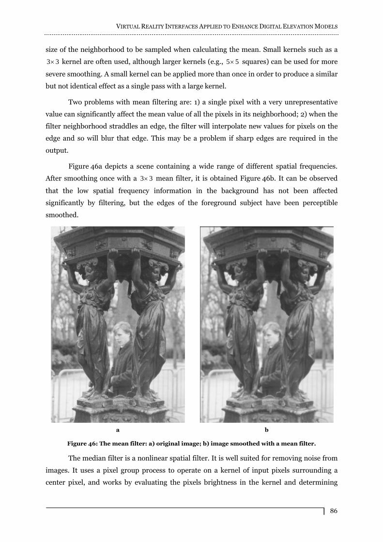
VIRTUAL REALITY INTERFACES APPLIED TO ENHANCE DIGITAL ELEVATION MODELS
86
size of the neighborhood to be sampled when calculating the mean. Small kernels such as a
33 kernel are often used, although larger kernels (e.g., 55 squares) can be used for more
severe smoothing. A small kernel can be applied more than once in order to produce a similar
but not identical effect as a single pass with a large kernel.
Two problems with mean filtering are: 1) a single pixel with a very unrepresentative
value can significantly affect the mean value of all the pixels in its neighborhood; 2) when the
filter neighborhood straddles an edge, the filter will interpolate new values for pixels on the
edge and so will blur that edge. This may be a problem if sharp edges are required in the
output.
Figure 46a depicts a scene containing a wide range of different spatial frequencies.
After smoothing once with a 33 mean filter, it is obtained Figure 46b. It can be observed
that the low spatial frequency information in the background has not been affected
significantly by filtering, but the edges of the foreground subject have been perceptible
smoothed.
a
b
Figure 46: The mean filter: a) original image; b) image smoothed with a mean filter.
The median filter is a nonlinear spatial filter. It is well suited for removing noise from
images. It uses a pixel group process to operate on a kernel of input pixels surrounding a
center pixel, and works by evaluating the pixels brightness in the kernel and determining

VIRTUAL REALITY INTERFACES APPLIED TO ENHANCE DIGITAL ELEVATION MODELS
87
which pixel brightness value is the median value of all pixels. The median value is determined
by placing the pixels brightness in ascending order and selecting the center value so that an
equal number of pixels brightness are less than, and greater than, the center value. The
median filter cleans up images with bright noise spikes, because the bright pixels tend to end
up the top of the ascending order of pixels in each pixel group. As a result, the bright spikes
are replaced by the median values of the group.
For example, consider the 55 matrix representing an image illustrated in Figure 47,
with ordered kernel values 150,127,126,125,124,123,120,119,115 . Calculating the median value of
the pixel kernel, the central pixel value of 150 is rather unrepresentative of the surrounding
pixels and is replaced with the median value 124 . A 33 kernel is used in this example;
larger kernels will produce more severe smoothing.
123 125 126 130 140
122 124 126 127 135
118 120 150 125 134
119 115 119 123 133
111 116 110 120 130
Figure 47: Illustrating the functioning of a median filter.
The median filter has two main advantages: 1) the median is a more robust average
than the mean and so a single very unrepresentative pixel in a pixel group will not affect the
median value significantly; 2) since the median value must actually be the value of one of the
pixels in the kernel, the median filter does not create new unrealistic pixel values when the
filter straddles an edge. For this reason the median filter is much better at preserving sharp
edges than the mean filter.
In order to illustrate the use of the median filter, consider the original image shown in
Figure 48a, corrupted with salt and pepper noise (bits have been flipped with probability 5%)
(see Figure 48b). After smoothing with a 33 filter, most of the noise has been eliminated, as
can be observed in Figure 48c.
If the image would be smoothed with a larger median filter, for example a 77
median filter, all the noisy pixels would disappear, but the image would look a bit imperfect,
as gray level regions are mapped together. Alternatively, the 33 median filter could be
passed over the image three times in order to remove all the noise with less loss of detail.

VIRTUAL REALITY INTERFACES APPLIED TO ENHANCE DIGITAL ELEVATION MODELS
88
a
b
c
Figure 48: Median filter: a) original image; b) salt and pepper noise; c) smoothed.
The sigma filter smoothes noise, preserves edges, and can leave lines untouched. This
filter works computing for each pixel in the input image the mean value of a set of pixels
within sigmavalue2 of the pixel of interest. Only pixels with a preliminary specified
neighborhood are considered in the calculation. If too few points within the local
neighborhood lie within the sigmavalue2 , then the pixel of interest is left unchanged,
otherwise, the calculated mean value is assigned to the output pixel. The sigma value, for a
given window, is computed as 2
2
Óx
ó .
Taubin has proposed a smoothing algorithm called ìë to smooth polygonal
meshes [TAUBIN, 2000]. This algorithm solves the problem of shrinkage presented by the
Laplacian smoothing algorithm. Laplacian smoothing is an iterative process, where in each
step every vertex of the mesh is moved to the barycenter of its neighbors. When Laplacian
smoothing is applied to a noisy 3D polygonal mesh without constraints, noise is removed, but
significant shape distortion may be introduced. Laplacian smoothing produces shrinkage,
because at the limit, all the vertices of the mesh converge to their barycenter.
The ìë algorithm uses the second degree transfer function kìkëkf 11 to
solve the problem of shrinkage. It can be implemented as two consecutive steps of Laplacian
smoothing with different scaling factors: the first one with 0ë , and the second one with
0 ëì . That is, after the Laplacian smoothing step with positive scale factor ë is
performed (shrinking step), a second Laplacian smoothing step with negative scale factor ì
is performed (unshrinking step).

VIRTUAL REALITY INTERFACES APPLIED TO ENHANCE DIGITAL ELEVATION MODELS
89
5.3.4.6 MODIFYING MINIMUM AND MAXIMUM HEIGHT VALUES
The user can edit the minimum and maximum values of the DEM. The input of the
new value can be done specifying directly a height value to be assigned to the DEM, or
modifying interactively this value and visualizing the result on the virtual DEM, until the
desired height is accomplished.
The user can modify the marginal height values of the terrain only for visualization
purposes, or he/she may cut out the values from the dataset less than (minimum
modification) the minimum value specified by the user and greater than (maximum
modification) the maximum value specified by the user, if they do not correspond to the true
minimum/maximum elevations of the DEM.
5.4 SOME CONSIDERATIONS
The first consideration to be made is that the methods proposed in the literature to
identify errors in DEMs give priority to the automatic identification of errors using
specialized algorithms. The automatic detection of errors makes possible the identification of
specific types of error only, because the algorithms look for specific characteristics. Moreover,
the use of automatic detection algorithms may be an efficient way to identify errors in terrain
models when the user does not know the data he/she is manipulating. But, if experienced
remote sensing data users are considered, which own an important background about their
data, the utilization of this knowledge in the identification process certainly implies in the
detection of any kind of errors possible in the DEM, making the identification process much
more efficient.
The methodology proposed by this thesis makes strong use of user�s knowledge about
DEM data, assisting him/her with visualization and interaction tools, as well as with
adequate analysis functions. Contact with experienced remote sensing data users has shown
that automation is not always desirable; users prefer visualize the data and errors will be
identified through visual interpretation supported by some statistical analysis.
A second consideration is that the methods actually applied to identify and remove
errors in DEMs are based on 2D interfaces. In this research work both, 2D and 3D interfaces
are applied to visualize and analyze terrain data in order to identify errors, and also to edit
data to remove incorrect elevation values. Indeed, 3D interfaces are widely used to visualize
terrain models, but yet are rarely utilized to resolve practical problems of remote sensing data
users.
Finally, an important differential of this thesis is that the implementation of the
proposed methodology resulted in a system to identify and remove errors in DEMs, as well as
VIRTUAL REALITY INTERFACES APPLIED TO ENHANCE DIGITAL ELEVATION MODELS
90
to visualize and analyze data in two and three dimensions.
5.5 FINAL REMARKS
The methodology presented in this chapter intends to make possible the identification
and correction of errors in DEMs, in order to enhance their precision (the correction is made
using known true height values), accuracy and reliability. Although this is the main goal of
this thesis, the user can apply the methodology to perform other enhancements to the
models, according to his/her interests.
The proposed methodology is a combination of visualization and interaction
techniques, analysis functions and editing methods. Since the objects of study are the DEMs,
all components of the methodology were carefully selected and adapted to manipulate this
specific type of data. In this way, the methodology can be seen as a specification of a
framework for DEM based applications.
CHAPTER 6
DEMEDITOR: A VIRTUAL REALITY BASED SYSTEM
TO VISUALIZE, ANALYZE AND EDIT DEMS
6.1 INTRODUCTION TO THE CHAPTER
Chapter 5 described the methodology proposed by this thesis to tackle the problem of
correcting elevation errors in DEMs; this chapter describes the DEMEditor, a system that
implements this methodology.
The DEMEditor is a system for visualizing, analyzing and editing DEMs. It is a
desktop VR based system, which reconstructs real-world terrain in VR. The virtual
environment is meant to be a place where specialized SAR data users explore and analyze
their large amounts of data, validate them according to known quality parameters and make
corrections on the DEM. Although the methodology is based on a 3D interface to enhance
DEMs, the DEMEditor offers, moreover the 3D one, a 2D interface to perform visualization,
analysis and editing. This approach makes the DEMEditor a complete software, offering the
user the 2D environment already known by the remote sensing community to manipulate its
data, and the 3D interface that brings realism and interaction.
The system is composed of four modules: the presentation module, the representation
module, the analysis module, and the editing module. Each of them implements specific
functionalities. This modular development makes it easy to add new functions to the system,
such as analysis or editing ones.
This chapter also gives an insight into some relevant implementation issues taken into
account during the development of the DEMEditor. Resolution, performance, realism and
interaction are briefly discussed in the context of this work.
6.2 INTRODUCING THE DEMEDITOR
The DEMEditor, as the name already suggests, is a system to edit DEMs in order to
enhance them. Beyond, the user may also use it to visualize and analyze DEM data. A set of
requirements were collected and specified during the development of the DEMEditor, to
define a user-friendly interface for the system and implement a tool that attends expert
remote sensing data users� expectations. A prototype was developed and made available to
such users, which provided an important feedback about the efficiency of the editor, and
allowed the test and enhancement of consistency and robustness of the software, as well as
the adding of new required functionalities.
DEMEDITOR: A VIRTUAL REALITY BASED SYSTEM TO VISUALIZE, ANALYZE AND EDIT DEMS
92
A non-immersive approach has been chosen to implement the DEMEditor, taking
quickly evolving technology into consideration (e.g., processing and display technologies), as
well as the need for using low cost technology in order to match customer�s interests. The
goal of bringing realistic, real-time technology to desktop computers has challenged the VR
community. Desktop VR is increasingly becoming an attractive option because of its ability to
build low cost realistic and interactive environments that can be deployed across every office.
The DEMEditor builds and manipulates desktop VR models based on InSAR DEMs. It
can be used with a common personal computer and with default input and output devices for
interaction (monitor, and keyboard and mouse). Using ordinary monitors to display VR
environments has some advantages: they are least expensive in terms of additional hardware
over other output devices, have good resolution, and the user can take advantage of keyboard
and mouse. Obviously, their main disadvantage is that they are not immersive. The keyboard
is a discrete input device. It simply generates one event at a time, based on the user; when
he/she presses a button an event is generated that is usually a Boolean value stating whether
the button was pressed down or released. The mouse is a more flexible combination/hybrid
input device that combines both discrete and continuous event generation. Continuous input
devices generate a continual stream of events in isolation (no user manipulation) or in
response to user action.
Using 2D interaction devices offers some advantages (very accurate, picking objects is
much easier in two dimensions, some operations such as 3D modeling that are 3D in nature
are more easily done with a 2D input device) over 3D interaction devices for certain tasks to
be performed with the DEMEditor. If haptic or tactile devices are not present, 2D interaction
on a physical surface provides a sense of feedback that is especially useful for drawing and
annotating. On the other hand, manipulate 3D objects with 2D interaction devices is least
natural.
The system is implemented in IDL version 5.x, a language developed by Research
Systems, Inc. The remote sensing community largely uses IDL, as it offers a number of built
in functions for image analysis and visualization. The DEMEditor runs across the Linux and
Microsoft Windows platforms, but only the Linux version has been tested for consistency and
robustness. Since IDL programs run across these platforms with some modifications, there
may occur errors when IDL�s portability fails.
IDL supports a graphics mode called �object graphics�, which uses an object-oriented
approach to create graphics objects, which must then be drawn, explicitly, to a specified
destination (for example, a window). IDL organizes a group of graphics objects into a
hierarchy or tree, which may contain scene, viewgroup, view, model, and atomic graphics
objects (graphics atoms). A graphics tree may have any number of branches, each of which in
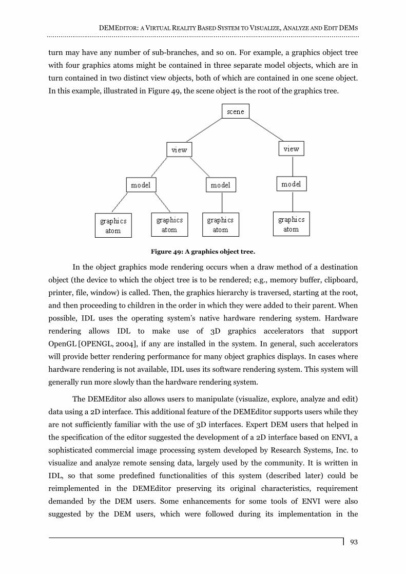
DEMEDITOR: A VIRTUAL REALITY BASED SYSTEM TO VISUALIZE, ANALYZE AND EDIT DEMS
93
turn may have any number of sub-branches, and so on. For example, a graphics object tree
with four graphics atoms might be contained in three separate model objects, which are in
turn contained in two distinct view objects, both of which are contained in one scene object.
In this example, illustrated in Figure 49, the scene object is the root of the graphics tree.
Figure 49: A graphics object tree.
In the object graphics mode rendering occurs when a draw method of a destination
object (the device to which the object tree is to be rendered; e.g., memory buffer, clipboard,
printer, file, window) is called. Then, the graphics hierarchy is traversed, starting at the root,
and then proceeding to children in the order in which they were added to their parent. When
possible, IDL uses the operating system�s native hardware rendering system. Hardware
rendering allows IDL to make use of 3D graphics accelerators that support
OpenGL [OPENGL, 2004], if any are installed in the system. In general, such accelerators
will provide better rendering performance for many object graphics displays. In cases where
hardware rendering is not available, IDL uses its software rendering system. This system will
generally run more slowly than the hardware rendering system.
The DEMEditor also allows users to manipulate (visualize, explore, analyze and edit)
data using a 2D interface. This additional feature of the DEMEditor supports users while they
are not sufficiently familiar with the use of 3D interfaces. Expert DEM users that helped in
the specification of the editor suggested the development of a 2D interface based on ENVI, a
sophisticated commercial image processing system developed by Research Systems, Inc. to
visualize and analyze remote sensing data, largely used by the community. It is written in
IDL, so that some predefined functionalities of this system (described later) could be
reimplemented in the DEMEditor preserving its original characteristics, requirement
demanded by the DEM users. Some enhancements for some tools of ENVI were also
suggested by the DEM users, which were followed during its implementation in the
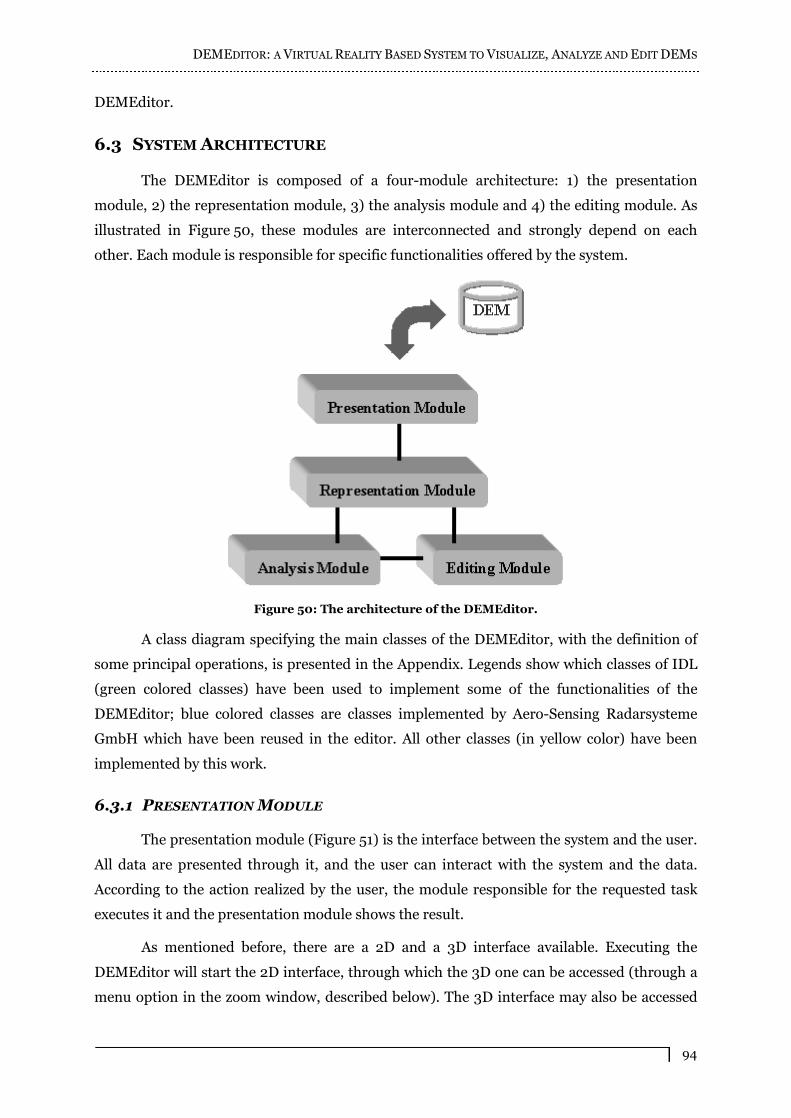
DEMEDITOR: A VIRTUAL REALITY BASED SYSTEM TO VISUALIZE, ANALYZE AND EDIT DEMS
94
DEMEditor.
6.3 SYSTEM ARCHITECTURE
The DEMEditor is composed of a four-module architecture: 1) the presentation
module, 2) the representation module, 3) the analysis module and 4) the editing module. As
illustrated in Figure 50, these modules are interconnected and strongly depend on each
other. Each module is responsible for specific functionalities offered by the system.
Figure 50: The architecture of the DEMEditor.
A class diagram specifying the main classes of the DEMEditor, with the definition of
some principal operations, is presented in the Appendix. Legends show which classes of IDL
(green colored classes) have been used to implement some of the functionalities of the
DEMEditor; blue colored classes are classes implemented by Aero-Sensing Radarsysteme
GmbH which have been reused in the editor. All other classes (in yellow color) have been
implemented by this work.
6.3.1 PRESENTATION MODULE
The presentation module (Figure 51) is the interface between the system and the user.
All data are presented through it, and the user can interact with the system and the data.
According to the action realized by the user, the module responsible for the requested task
executes it and the presentation module shows the result.
As mentioned before, there are a 2D and a 3D interface available. Executing the
DEMEditor will start the 2D interface, through which the 3D one can be accessed (through a
menu option in the zoom window, described below). The 3D interface may also be accessed
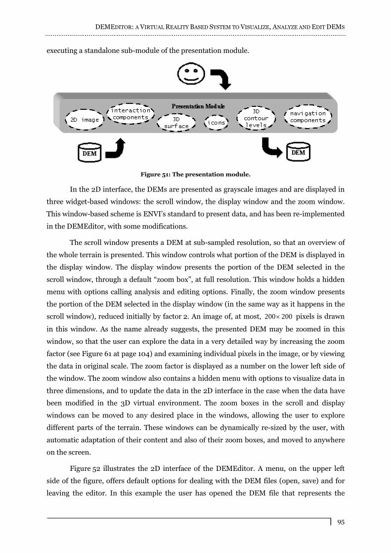
DEMEDITOR: A VIRTUAL REALITY BASED SYSTEM TO VISUALIZE, ANALYZE AND EDIT DEMS
95
executing a standalone sub-module of the presentation module.
Figure 51: The presentation module.
In the 2D interface, the DEMs are presented as grayscale images and are displayed in
three widget-based windows: the scroll window, the display window and the zoom window.
This window-based scheme is ENVI�s standard to present data, and has been re-implemented
in the DEMEditor, with some modifications.
The scroll window presents a DEM at sub-sampled resolution, so that an overview of
the whole terrain is presented. This window controls what portion of the DEM is displayed in
the display window. The display window presents the portion of the DEM selected in the
scroll window, through a default �zoom box�, at full resolution. This window holds a hidden
menu with options calling analysis and editing options. Finally, the zoom window presents
the portion of the DEM selected in the display window (in the same way as it happens in the
scroll window), reduced initially by factor 2. An image of, at most, 200200 pixels is drawn
in this window. As the name already suggests, the presented DEM may be zoomed in this
window, so that the user can explore the data in a very detailed way by increasing the zoom
factor (see Figure 61 at page 104) and examining individual pixels in the image, or by viewing
the data in original scale. The zoom factor is displayed as a number on the lower left side of
the window. The zoom window also contains a hidden menu with options to visualize data in
three dimensions, and to update the data in the 2D interface in the case when the data have
been modified in the 3D virtual environment. The zoom boxes in the scroll and display
windows can be moved to any desired place in the windows, allowing the user to explore
different parts of the terrain. These windows can be dynamically re-sized by the user, with
automatic adaptation of their content and also of their zoom boxes, and moved to anywhere
on the screen.
Figure 52 illustrates the 2D interface of the DEMEditor. A menu, on the upper left
side of the figure, offers default options for dealing with the DEM files (open, save) and for
leaving the editor. In this example the user has opened the DEM file that represents the
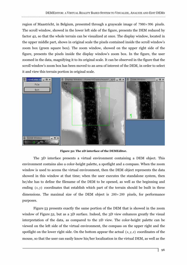
DEMEDITOR: A VIRTUAL REALITY BASED SYSTEM TO VISUALIZE, ANALYZE AND EDIT DEMS
96
region of Maastricht, in Belgium, presented through a grayscale image of 9967980 pixels.
The scroll window, showed in the lower left side of the figure, presents the DEM reduced by
factor 42, so that the whole terrain can be visualized at once. The display window, located in
the upper middle part, shows in original scale the pixels contained inside the scroll window�s
zoom box (green square box). The zoom window, showed on the upper right side of the
figure, presents the pixels inside the display window�s zoom box. In the figure, the user
zoomed in the data, magnifying it to its original scale. It can be observed in the figure that the
scroll window�s zoom box has been moved to an area of interest of the DEM, in order to select
it and view this terrain portion in original scale.
Figure 52: The 2D interface of the DEMEditor.
The 3D interface presents a virtual environment containing a DEM object. This
environment contains also a color-height palette, a spotlight and a compass. When the zoom
window is used to access the virtual environment, then the DEM object represents the data
showed in this window at that time; when the user executes the standalone system, then
he/she has to define the filename of the DEM to be opened, as well as the beginning and
ending ),( yx coordinates that establish which part of the terrain should be built in three
dimensions. The maximal size of the DEM object is 200200 pixels, for performance
purposes.
Figure 53 presents exactly the same portion of the DEM that is showed in the zoom
window of Figure 52, but as a 3D surface. Indeed, the 3D view enhances greatly the visual
interpretation of the data, as compared to the 2D view. The color-height palette can be
viewed on the left side of the virtual environment, the compass on the upper right and the
spotlight on the lower right side. On the bottom appear the actual ),,( zyx coordinates of the
mouse, so that the user can easily know his/her localization in the virtual DEM, as well as the
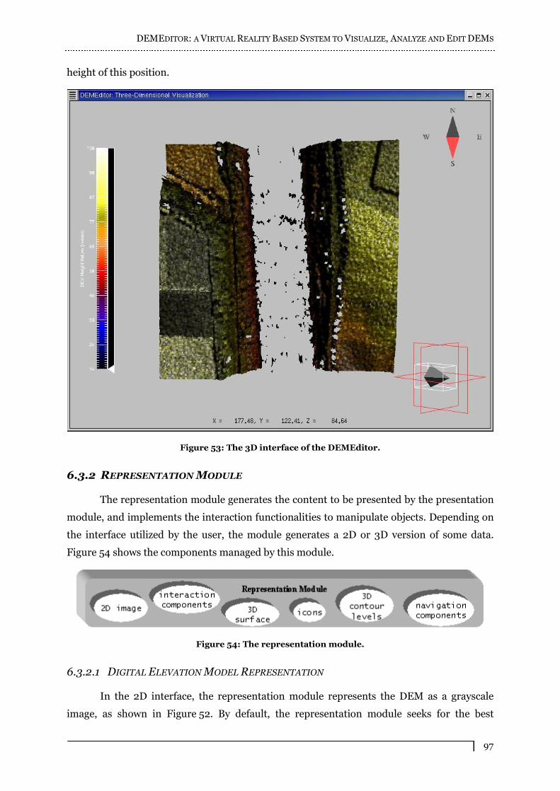
DEMEDITOR: A VIRTUAL REALITY BASED SYSTEM TO VISUALIZE, ANALYZE AND EDIT DEMS
97
height of this position.
Figure 53: The 3D interface of the DEMEditor.
6.3.2 REPRESENTATION MODULE
The representation module generates the content to be presented by the presentation
module, and implements the interaction functionalities to manipulate objects. Depending on
the interface utilized by the user, the module generates a 2D or 3D version of some data.
Figure 54 shows the components managed by this module.
Figure 54: The representation module.
6.3.2.1 DIGITAL ELEVATION MODEL REPRESENTATION
In the 2D interface, the representation module represents the DEM as a grayscale
image, as shown in Figure 52. By default, the representation module seeks for the best

DEMEDITOR: A VIRTUAL REALITY BASED SYSTEM TO VISUALIZE, ANALYZE AND EDIT DEMS
98
contrast for the dataset when the file is opened or reloaded by the system: the optimal
minimum and maximum values for the image are identified by the system, which are used to
scale all values of the dataset that lie in the range )maximumminimum( x into the range
)top0( x . The top range represents the maximum value of the scaled result, which is
specified as 255 by the system. The minimum value of the scaled result is always 0 . All
values greater or equal to maximum are set equal to top in the result, all values less than or
equal to minimum are set equal to 0 , and intermediary values are slid (a constant brightness
value is added to or subtracted from all pixels) and stretched (all pixels are multiplied or
divided by a constant value) to redistribute the brightness values in the image.
Figure 55: The DEM surface rendered as a wire mesh object.
In the 3D interface, the representation module constructs a default virtual
environment that contains a 3D surface representing part of a DEM (see Figure 53). This
object is rendered by the system as a solid surface. The user may control how the surface is
rendered, to display, for example, a single pixel for each data point of the surface, the surface
as a wire mesh, the surface using only lines drawn parallel to the x -axis or the y -axis, or a
wire mesh or a solid lego-type surface (similar to a histogram plot). Figure 55 illustrates a

DEMEDITOR: A VIRTUAL REALITY BASED SYSTEM TO VISUALIZE, ANALYZE AND EDIT DEMS
99
surface rendered as a wire mesh. The rendering quality at which data are to be drawn to the
window is by default set as medium, but it can be set as low or high by the user.
Two types of shading can be used: flat shading or Gouraud shading (default). In flat
shading the color of the first vertex in the surface is used to define the color for the entire
surface. The color has a constant intensity. In Gouraud shading each polygon is shaded by
using linear interpolation of vertex intensities along each edge and then between edges along
each scan line. Gouraud shading may be slower than flat shading, but results in a smoother
appearance. If a light source (not an ambient light) is not supplied in the scene, the solid
surface object will appear flat with either flat or Gouraud shading. Therefore, the virtual
environment constructed by the representation module uses a permanent directional light to
illuminate the scene. The surface illustrated in Figure 53 uses Gouraud shading and the
virtual environment is illuminated by a directional light source.
By default, the representation module, in order to represent point and wire frame
surfaces, does not draw the hidden lines (lines that are behind the visible parts of the
surface), but the user may require that these lines are rendered. The control of the rendering
style and quality, the shading, and the hidden lines is performed through a widget-based
menu interface showed in Figure 62a.
In the 3D interface, the user may also zoom a specific area of the virtual DEM, as
illustrated in Figure 56. The generation of the zoomed surface object is done in the same way
as the construction of the original DEM surface, explained above. The zoomed surface
illustrated below presents the terrain area selected with a zoom box icon in Figure 59.
Figure 56: Zoomed 3D surface.

DEMEDITOR: A VIRTUAL REALITY BASED SYSTEM TO VISUALIZE, ANALYZE AND EDIT DEMS
100
The representation of the DEM with contour levels is performed creating an object
derived from the DEM data. The system selects the elevation values to be plotted according to
the number of contour levels required, in real-time, by the user. The contour levels object is
placed in the virtual environment, so that a compound view composed by the surface and the
contour levels is created. The user can also select the color to be used to draw the lines.
Figure 57 illustrates this form of representation, where the user has required a contour levels
representation with 30 lines, to be drawn in blue color. This object can be added to/removed
from the virtual environment by switching on/off the contour levels option in a menu (see
Figure 62a).
Figure 57: Compound visualization of a DEM in the virtual environment.
The representation of height values through colors is implemented applying a vector
of colors (RGB values) to each vertex of the 3D surface in turn. If there are more vertices than
colors supplied, the system will cycle through the colors. The DEMEditor allows the user to
select a predefined color table to serve as colors vector to be applied to the vertices of the
surface. Figure 57 illustrates an example were the elevations are presented in a gradient
starting with the blue color (low height values) and ending with the yellow color (high height
values). Vertex colors may be switched on/off by the user through an option in a menu
contour
levels
parameters
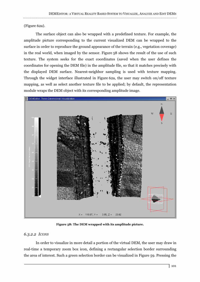
DEMEDITOR: A VIRTUAL REALITY BASED SYSTEM TO VISUALIZE, ANALYZE AND EDIT DEMS
101
(Figure 62a).
The surface object can also be wrapped with a predefined texture. For example, the
amplitude picture corresponding to the current visualized DEM can be wrapped to the
surface in order to reproduce the ground appearance of the terrain (e.g., vegetation coverage)
in the real world, when imaged by the sensor. Figure 58 shows the result of the use of such
texture. The system seeks for the exact coordinates (saved when the user defines the
coordinates for opening the DEM file) in the amplitude file, so that it matches precisely with
the displayed DEM surface. Nearest-neighbor sampling is used with texture mapping.
Through the widget interface illustrated in Figure 62a, the user may switch on/off texture
mapping, as well as select another texture file to be applied; by default, the representation
module wraps the DEM object with its corresponding amplitude image.
Figure 58: The DEM wrapped with its amplitude picture.
6.3.2.2 ICONS
In order to visualize in more detail a portion of the virtual DEM, the user may draw in
real-time a temporary zoom box icon, defining a rectangular selection border surrounding
the area of interest. Such a green selection border can be visualized in Figure 59. Pressing the

DEMEDITOR: A VIRTUAL REALITY BASED SYSTEM TO VISUALIZE, ANALYZE AND EDIT DEMS
102
right mouse button over the virtual DEM and moving it, the zoom box is drawn; releasing the
button, the zoom box is destroyed and a window presenting a virtual environment equal to
the original one is created, showing a 3D surface object generated from the data selected by
the zoom box icon (see Figure 56). All functionalities included by the original virtual
environment are implemented in the same way in the zoomed scene. The user can also select
the color to be used to draw the zoom box.
Figure 59: Zooming the surface using a zoom box icon.
The color-height palette is an icon that represents a color bar indicating the height
variations of the terrain (see left side of Figure 59). This indication helps the user to
understand what the colors mapped to the terrain�s vertices mean, since they are associated
to corresponding height values in the palette. If a vector of colors is applied to the vertices of
the 3D surface, these colors are shown in the color bar (see Figure 57), and if an amplitude
image wraps the surface, the palette presents the gray levels of the image as illustrated in
Figure 58. In the case where the surface is presented without a texture and no colors are
mapped to the vertices, it appears as a white colored object, and the color-height palette will
present height variations also in white color, according to the surface.
zoom box
icon
parameters
color-height palette
icon
spotlight
icon
compass
icon
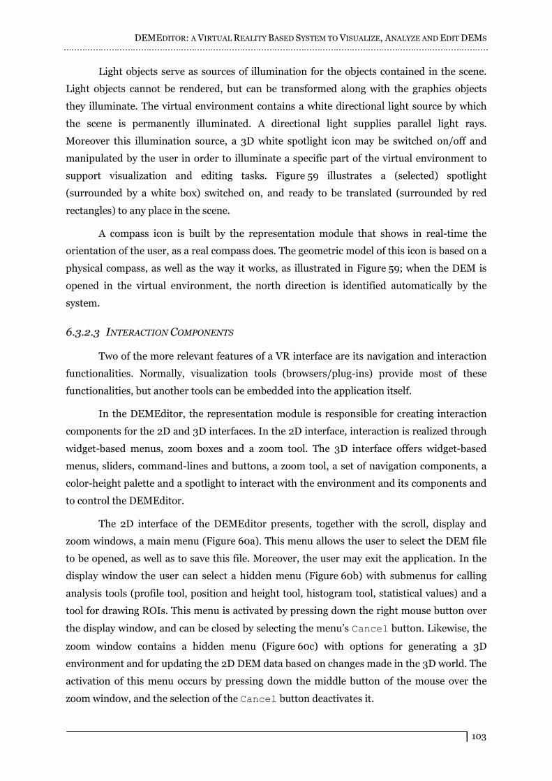
DEMEDITOR: A VIRTUAL REALITY BASED SYSTEM TO VISUALIZE, ANALYZE AND EDIT DEMS
103
Light objects serve as sources of illumination for the objects contained in the scene.
Light objects cannot be rendered, but can be transformed along with the graphics objects
they illuminate. The virtual environment contains a white directional light source by which
the scene is permanently illuminated. A directional light supplies parallel light rays.
Moreover this illumination source, a 3D white spotlight icon may be switched on/off and
manipulated by the user in order to illuminate a specific part of the virtual environment to
support visualization and editing tasks. Figure 59 illustrates a (selected) spotlight
(surrounded by a white box) switched on, and ready to be translated (surrounded by red
rectangles) to any place in the scene.
A compass icon is built by the representation module that shows in real-time the
orientation of the user, as a real compass does. The geometric model of this icon is based on a
physical compass, as well as the way it works, as illustrated in Figure 59; when the DEM is
opened in the virtual environment, the north direction is identified automatically by the
system.
6.3.2.3 INTERACTION COMPONENTS
Two of the more relevant features of a VR interface are its navigation and interaction
functionalities. Normally, visualization tools (browsers/plug-ins) provide most of these
functionalities, but another tools can be embedded into the application itself.
In the DEMEditor, the representation module is responsible for creating interaction
components for the 2D and 3D interfaces. In the 2D interface, interaction is realized through
widget-based menus, zoom boxes and a zoom tool. The 3D interface offers widget-based
menus, sliders, command-lines and buttons, a zoom tool, a set of navigation components, a
color-height palette and a spotlight to interact with the environment and its components and
to control the DEMEditor.
The 2D interface of the DEMEditor presents, together with the scroll, display and
zoom windows, a main menu (Figure 60a). This menu allows the user to select the DEM file
to be opened, as well as to save this file. Moreover, the user may exit the application. In the
display window the user can select a hidden menu (Figure 60b) with submenus for calling
analysis tools (profile tool, position and height tool, histogram tool, statistical values) and a
tool for drawing ROIs. This menu is activated by pressing down the right mouse button over
the display window, and can be closed by selecting the menu�s Cancel button. Likewise, the
zoom window contains a hidden menu (Figure 60c) with options for generating a 3D
environment and for updating the 2D DEM data based on changes made in the 3D world. The
activation of this menu occurs by pressing down the middle button of the mouse over the
zoom window, and the selection of the Cancel button deactivates it.
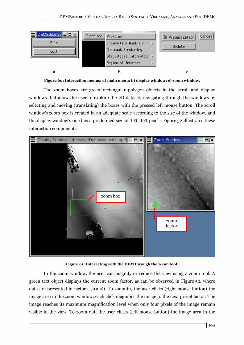
DEMEDITOR: A VIRTUAL REALITY BASED SYSTEM TO VISUALIZE, ANALYZE AND EDIT DEMS
104
a b c
Figure 60: Interaction menus: a) main menu; b) display window; c) zoom window.
The zoom boxes are green rectangular polygon objects in the scroll and display
windows that allow the user to explore the 2D dataset, navigating through the windows by
selecting and moving (translating) the boxes with the pressed left mouse button. The scroll
window�s zoom box is created in an adequate scale according to the size of the window, and
the display window�s one has a predefined size of 100100 pixels. Figure 52 illustrates these
interaction components.
Figure 61: Interacting with the DEM through the zoom tool.
In the zoom window, the user can magnify or reduce the view using a zoom tool. A
green text object displays the current zoom factor, as can be observed in Figure 52, where
data are presented in factor 1 (100%). To zoom in, the user clicks (right mouse button) the
image area in the zoom window; each click magnifies the image to the next preset factor. The
image reaches its maximum magnification level when only four pixels of the image remain
visible in the view. To zoom out, the user clicks (left mouse button) the image area in the
zoom box
zoom
factor

DEMEDITOR: A VIRTUAL REALITY BASED SYSTEM TO VISUALIZE, ANALYZE AND EDIT DEMS
105
zoom window; each click reduces the view to the previous preset factor. Factor 1 corresponds
to the maximum reduction level, where the image appears at full resolution. The zoom tool
affects directly the zoom box of the display window, which is automatically rescaled
according to the zoom factor; after the zoom box is rescaled, the pixels selected by the box are
updated in the zoom window. Figure 61 illustrates this interaction process, where the content
of the zoom window has been reduced by factor 4, which corresponds to a zoom percentage
of 25%. The rescaling of the zoom box of the display window can be observed, when
comparing Figure 61 to Figure 52.
In the 3D interface, widgets, illustrated in Figure 62a, are used to control the 3D
presentation of the DEM (rendering style, drag quality, shading, hidden lines, vertex colors,
texture mapping, contour levels, minimum and maximum height values control), as well as to
choose some interaction (viewpoints, walk/pan) and analysis components (minimum and
maximum values, mean, variance, skewness and kurtosis values, histogram, profile), and call
the editing menu (see Figure 62b) and exit the environment.
a b
Figure 62: Interacting with the 3D environment: a) options menu; b) editing menu.
Hidden widgets displaying parameters to be adjusted to control the contour levels
object (bottom part of Figure 57) and the zoom tool (bottom part of Figure 59) are also
automatically activated by the system when the user requires these functionalities.
Object selection in the DEMEditor was simple to implement, because IDL allows that
by the creation of an object it is configured as selectable or not. Therefore, if the user presses
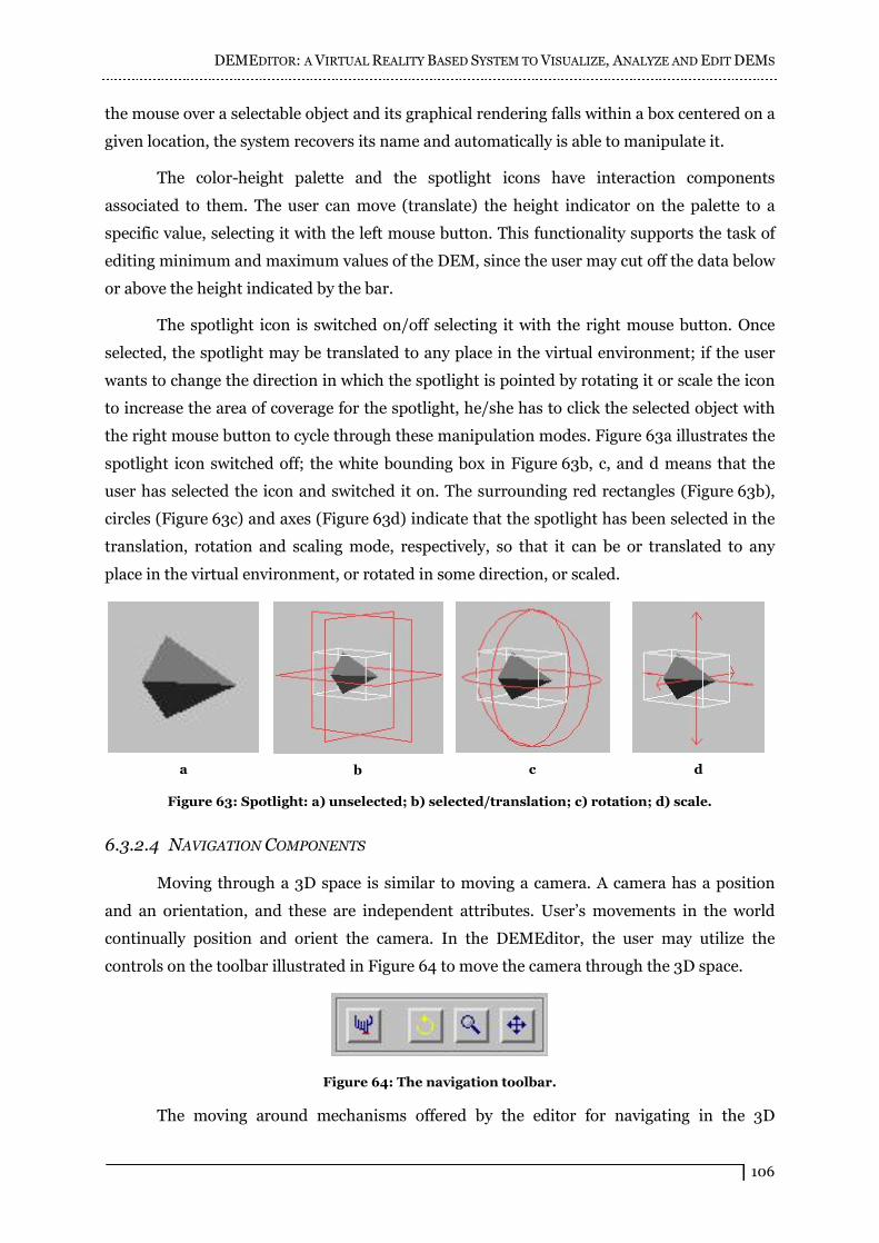
DEMEDITOR: A VIRTUAL REALITY BASED SYSTEM TO VISUALIZE, ANALYZE AND EDIT DEMS
106
the mouse over a selectable object and its graphical rendering falls within a box centered on a
given location, the system recovers its name and automatically is able to manipulate it.
The color-height palette and the spotlight icons have interaction components
associated to them. The user can move (translate) the height indicator on the palette to a
specific value, selecting it with the left mouse button. This functionality supports the task of
editing minimum and maximum values of the DEM, since the user may cut off the data below
or above the height indicated by the bar.
The spotlight icon is switched on/off selecting it with the right mouse button. Once
selected, the spotlight may be translated to any place in the virtual environment; if the user
wants to change the direction in which the spotlight is pointed by rotating it or scale the icon
to increase the area of coverage for the spotlight, he/she has to click the selected object with
the right mouse button to cycle through these manipulation modes. Figure 63a illustrates the
spotlight icon switched off; the white bounding box in Figure 63b, c, and d means that the
user has selected the icon and switched it on. The surrounding red rectangles (Figure 63b),
circles (Figure 63c) and axes (Figure 63d) indicate that the spotlight has been selected in the
translation, rotation and scaling mode, respectively, so that it can be or translated to any
place in the virtual environment, or rotated in some direction, or scaled.
a
b
c
d
Figure 63: Spotlight: a) unselected; b) selected/translation; c) rotation; d) scale.
6.3.2.4 NAVIGATION COMPONENTS
Moving through a 3D space is similar to moving a camera. A camera has a position
and an orientation, and these are independent attributes. User�s movements in the world
continually position and orient the camera. In the DEMEditor, the user may utilize the
controls on the toolbar illustrated in Figure 64 to move the camera through the 3D space.
Figure 64: The navigation toolbar.
The moving around mechanisms offered by the editor for navigating in the 3D
DEMEDITOR: A VIRTUAL REALITY BASED SYSTEM TO VISUALIZE, ANALYZE AND EDIT DEMS
107
environment are the study, the walk, and the pan modes (the second, third and fourth
buttons of the toolbar, respectively). The user can switch the navigation mode by clicking
buttons on the toolbar. The user can navigate with the mouse, choosing a navigation mode,
position the pointer anywhere in the 3D window and pressing the left mouse button, moving
the mouse while holding down its left button (the direction in which the user drags the mouse
determines the camera motion) and, finally, releasing the left mouse button to stop moving.
The distance that the user drags the mouse determines the speed with which the camera
moves.
The walk mode moves the camera closer or further in a horizontal plane. By moving
forward, the camera moves closer from the central point of the geometry in the 3D scene, and
by moving backward, the camera moves further. The study mode can be used to examine an
object from various angles. Forward, backward, right and left move the camera around the
central point that is defined by the center of bounding box of the geometry in the 3D scene.
The pan mode moves the camera up, down, left or right within a vertical plane. Forward
moves up, backward moves down, right moves right and left moves left.
A restore function (first button of the toolbar) returns automatically to the loaded
world�s original active viewpoint. This mechanism can help to re-orient a camera if the user
has lost his/her way in a world. Unlike the navigation modes, this button invokes a
predefined action that takes place as the user clicks on it.
The user can utilize a set of predefined viewpoints (available through the menu
interface showed in Figure 62a) to navigate through the virtual environment: perspective
view, overview, north-south, west-east, east-west and south-north views. The selection of one
of the viewpoints rotates the surface object about a specified axis by a specified angle. This
transformation moves the camera of the user and gives him/her the impression that he/she
moved in the scene, viewing the world from another position and orientation. For example, in
Figure 57 the user selected the overview point of view that allows the visualization of the
whole scene at once. Figure 55 shows a perspective view of the DEM.
6.3.3 ANALYSIS MODULE
The analysis module, as illustrated in Figure 65, contains components for drawing a
histogram and profile lines, for computing the mean, variance, skewness and kurtosis of the
actual dataset, for showing the height value of any position of the DEM, and for returning the
minimum and maximum height values of the terrain. When the user performs an analysis
task, the function responsible for that task is executed and managed by this module.
Additional analysis tools may be easily associated to this module in order to be used
with the DEMEditor, when other analysis and validation tasks will be required.
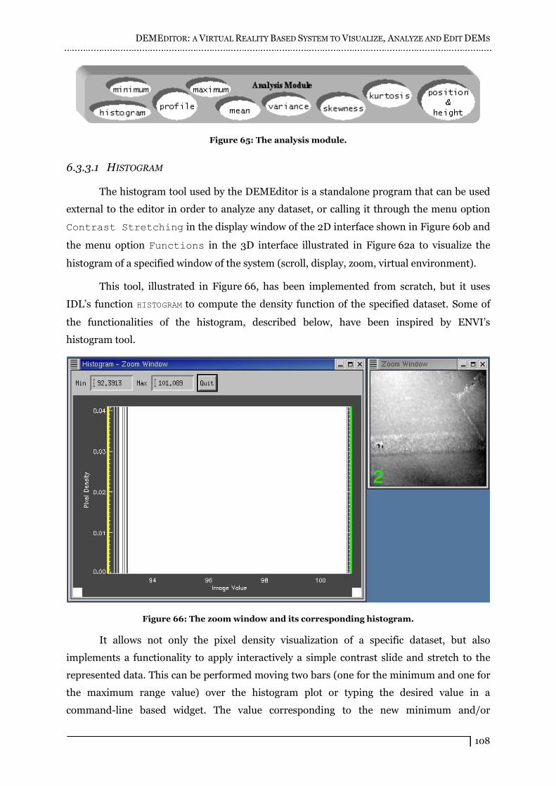
DEMEDITOR: A VIRTUAL REALITY BASED SYSTEM TO VISUALIZE, ANALYZE AND EDIT DEMS
108
Figure 65: The analysis module.
6.3.3.1 HISTOGRAM
The histogram tool used by the DEMEditor is a standalone program that can be used
external to the editor in order to analyze any dataset, or calling it through the menu option
Contrast Stretching in the display window of the 2D interface shown in Figure 60b and
the menu option Functions in the 3D interface illustrated in Figure 62a to visualize the
histogram of a specified window of the system (scroll, display, zoom, virtual environment).
This tool, illustrated in Figure 66, has been implemented from scratch, but it uses
IDL�s function HISTOGRAM to compute the density function of the specified dataset. Some of
the functionalities of the histogram, described below, have been inspired by ENVI�s
histogram tool.
Figure 66: The zoom window and its corresponding histogram.
It allows not only the pixel density visualization of a specific dataset, but also
implements a functionality to apply interactively a simple contrast slide and stretch to the
represented data. This can be performed moving two bars (one for the minimum and one for
the maximum range value) over the histogram plot or typing the desired value in a
command-line based widget. The value corresponding to the new minimum and/or
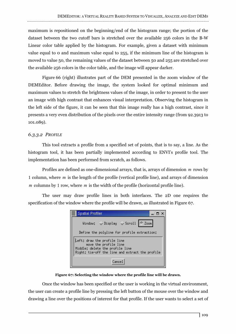
DEMEDITOR: A VIRTUAL REALITY BASED SYSTEM TO VISUALIZE, ANALYZE AND EDIT DEMS
109
maximum is repositioned on the beginning/end of the histogram range; the portion of the
dataset between the two cutoff bars is stretched over the available 256 colors in the B-W
Linear color table applied by the histogram. For example, given a dataset with minimum
value equal to 0 and maximum value equal to 255, if the minimum line of the histogram is
moved to value 50, the remaining values of the dataset between 50 and 255 are stretched over
the available 256 colors in the color table, and the image will appear darker.
Figure 66 (right) illustrates part of the DEM presented in the zoom window of the
DEMEditor. Before drawing the image, the system looked for optimal minimum and
maximum values to stretch the brightness values of the image, in order to present to the user
an image with high contrast that enhances visual interpretation. Observing the histogram in
the left side of the figure, it can be seen that this image really has a high contrast, since it
presents a very even distribution of the pixels over the entire intensity range (from 92.3913 to
101.089).
6.3.3.2 PROFILE
This tool extracts a profile from a specified set of points, that is to say, a line. As the
histogram tool, it has been partially implemented according to ENVI�s profile tool. The
implementation has been performed from scratch, as follows.
Profiles are defined as one-dimensional arrays, that is, arrays of dimension m rows by
1 column, where m is the length of the profile (vertical profile line), and arrays of dimension
m columns by 1 row, where m is the width of the profile (horizontal profile line).
The user may draw profile lines in both interfaces. The 2D one requires the
specification of the window where the profile will be drawn, as illustrated in Figure 67.
Figure 67: Selecting the window where the profile line will be drawn.
Once the window has been specified or the user is working in the virtual environment,
the user can create a profile line by pressing the left button of the mouse over the window and
drawing a line over the positions of interest for that profile. If the user wants to select a set of

DEMEDITOR: A VIRTUAL REALITY BASED SYSTEM TO VISUALIZE, ANALYZE AND EDIT DEMS
110
continuous points to create a profile line, he/she may release the mouse button, move the
mouse to the next desired point of the sequence and again press the left mouse button.
Pressing the right mouse button ties off the profile line and extracts the profile from the
points that compose the line; this profile is presented in a separate window, as can be
observed in Figure 68. In this figure have been drawn three profile lines, and the profile
window of the third one is shown.
a b
Figure 68: Profile: a) drawing the line; b) viewing graphically the height variations.
Pressing the left mouse button over a profile line selects it (makes it active). An active
line such as line #3 in Figure 68a, may be moved to any place of the window or deleted with
the middle mouse button. In the case the user moves the profile line to another positions in
the DEM, the analysis module automatically updates the profile according to the set of points
defined at the moment, allowing the user to observe interactively the profile changes in the
terrain. The analysis module can manage a maximum of ten profile lines at once.
The profile tool can be accessed through the menu option Profiles in the display
window of the 2D interface (Figure 60b) and the menu option Functions in the 2D widget-
based interface of the 3D interface (Figure 62a). In this interface the profile tool goes along
with the terrain, according to its height at each position, which enhances comprehension
about the profile of the set of points being analyzed.
6.3.3.3 STATISTICAL INFORMATION
The mean, variance, skewness and kurtosis tools return the mean, variance, skewness
and kurtosis, respectively, of the current dataset. They call IDL�s function named MOMENT,
which computes the mean, variance, skewness and kurtosis of a sample population contained
inactive
profile
lines #1
and #2
selected
profile line #3
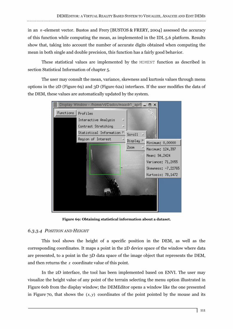
DEMEDITOR: A VIRTUAL REALITY BASED SYSTEM TO VISUALIZE, ANALYZE AND EDIT DEMS
111
in an n -element vector. Bustos and Frery [BUSTOS & FRERY, 2004] assessed the accuracy
of this function while computing the mean, as implemented in the IDL 5.6 platform. Results
show that, taking into account the number of accurate digits obtained when computing the
mean in both single and double precision, this function has a fairly good behavior.
These statistical values are implemented by the MOMENT function as described in
section Statistical Information of chapter 5.
The user may consult the mean, variance, skewness and kurtosis values through menu
options in the 2D (Figure 69) and 3D (Figure 62a) interfaces. If the user modifies the data of
the DEM, these values are automatically updated by the system.
Figure 69: Obtaining statistical information about a dataset.
6.3.3.4 POSITION AND HEIGHT
This tool shows the height of a specific position in the DEM, as well as the
corresponding coordinates. It maps a point in the 2D device space of the window where data
are presented, to a point in the 3D data space of the image object that represents the DEM,
and then returns the z coordinate value of this point.
In the 2D interface, the tool has been implemented based on ENVI. The user may
visualize the height value of any point of the terrain selecting the menu option illustrated in
Figure 60b from the display window; the DEMEditor opens a window like the one presented
in Figure 70, that shows the ),( yx coordinates of the point pointed by the mouse and its

DEMEDITOR: A VIRTUAL REALITY BASED SYSTEM TO VISUALIZE, ANALYZE AND EDIT DEMS
112
corresponding z value. When the user moves the mouse over any of the windows, the
analysis module updates this information automatically.
Figure 70: The position and height visualization window.
In the virtual environment, the position-height information are presented on the
bottom of the environment window (see Figure 53), so that the user may manipulate the
virtual DEM (select, navigate, and so on) and always have precise information about the
coordinates of the mouse position and their corresponding height value.
6.3.3.5 MINIMUM AND MAXIMUM VALUES
The minimum and maximum tools, that call IDL�s functions named MINIMUM and
MAXIMUM, respectively, return the values of the smallest and largest elements of the DEM
array presented in a specified window. They basically seek the whole array and compare the
values until the minimum and maximum ones are found. These values are then returned by
the functions.
The minimum and maximum tools look automatically for the minimum and
maximum values of the dataset, and the user may consult these values through menu options
in the 2D (Figure 69) and 3D (Figure 62a) interfaces. The system keeps these values updated
if the user makes modifications on the data of the DEM.
6.3.4 EDITING MODULE
The editing module (see Figure 71) implements generally used editing methods, such
as selection, interpolation, cut, and smoothing. These tools allow users to remove elevation
errors from the DEM, smooth the terrain, modify the minimum and maximum values of a
dataset, and so on.
Figure 71: The editing module.
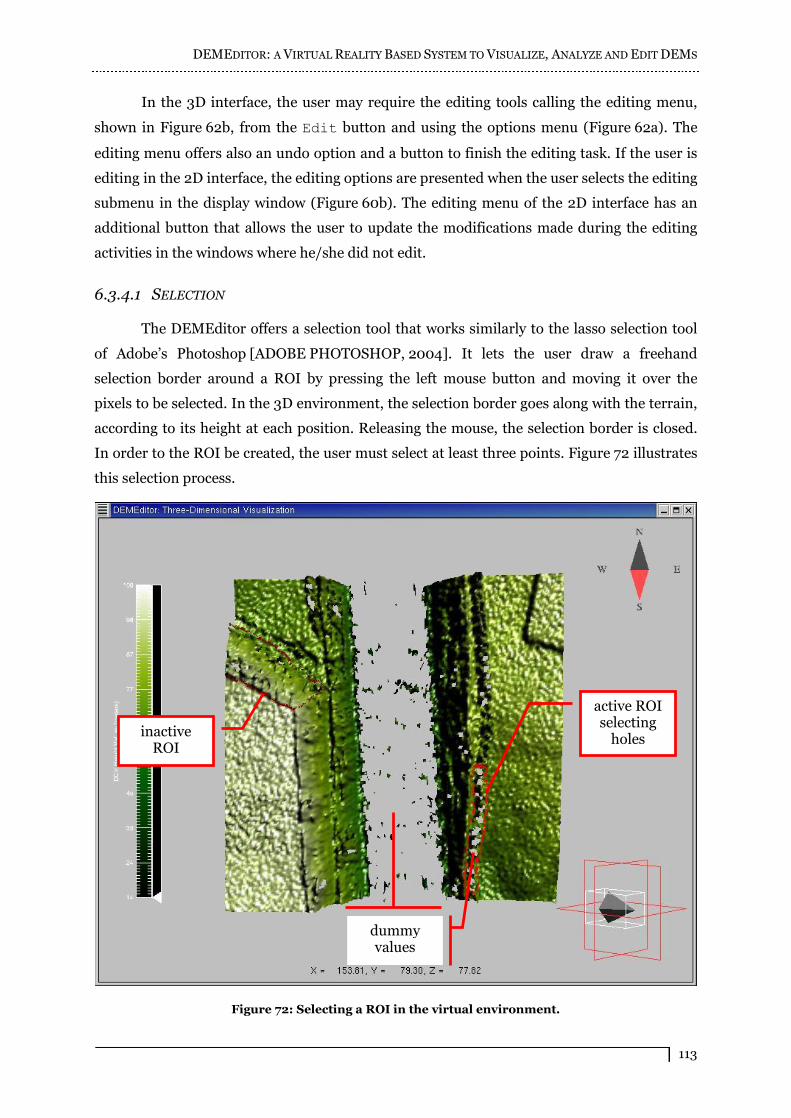
DEMEDITOR: A VIRTUAL REALITY BASED SYSTEM TO VISUALIZE, ANALYZE AND EDIT DEMS
113
In the 3D interface, the user may require the editing tools calling the editing menu,
shown in Figure 62b, from the Edit button and using the options menu (Figure 62a). The
editing menu offers also an undo option and a button to finish the editing task. If the user is
editing in the 2D interface, the editing options are presented when the user selects the editing
submenu in the display window (Figure 60b). The editing menu of the 2D interface has an
additional button that allows the user to update the modifications made during the editing
activities in the windows where he/she did not edit.
6.3.4.1 SELECTION
The DEMEditor offers a selection tool that works similarly to the lasso selection tool
of Adobe�s Photoshop [ADOBE PHOTOSHOP, 2004]. It lets the user draw a freehand
selection border around a ROI by pressing the left mouse button and moving it over the
pixels to be selected. In the 3D environment, the selection border goes along with the terrain,
according to its height at each position. Releasing the mouse, the selection border is closed.
In order to the ROI be created, the user must select at least three points. Figure 72 illustrates
this selection process.
Figure 72: Selecting a ROI in the virtual environment.
inactive
ROI
active ROI
selecting
holes
dummy
values
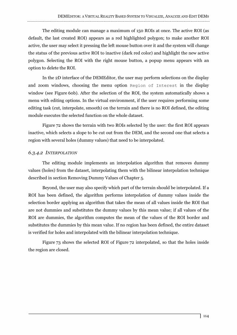
DEMEDITOR: A VIRTUAL REALITY BASED SYSTEM TO VISUALIZE, ANALYZE AND EDIT DEMS
114
The editing module can manage a maximum of 150 ROIs at once. The active ROI (as
default, the last created ROI) appears as a red highlighted polygon; to make another ROI
active, the user may select it pressing the left mouse button over it and the system will change
the status of the previous active ROI to inactive (dark red color) and highlight the new active
polygon. Selecting the ROI with the right mouse button, a popup menu appears with an
option to delete the ROI.
In the 2D interface of the DEMEditor, the user may perform selections on the display
and zoom windows, choosing the menu option Region of Interest in the display
window (see Figure 60b). After the selection of the ROI, the system automatically shows a
menu with editing options. In the virtual environment, if the user requires performing some
editing task (cut, interpolate, smooth) on the terrain and there is no ROI defined, the editing
module executes the selected function on the whole dataset.
Figure 72 shows the terrain with two ROIs selected by the user: the first ROI appears
inactive, which selects a slope to be cut out from the DEM, and the second one that selects a
region with several holes (dummy values) that need to be interpolated.
6.3.4.2 INTERPOLATION
The editing module implements an interpolation algorithm that removes dummy
values (holes) from the dataset, interpolating them with the bilinear interpolation technique
described in section Removing Dummy Values of Chapter 5.
Beyond, the user may also specify which part of the terrain should be interpolated. If a
ROI has been defined, the algorithm performs interpolation of dummy values inside the
selection border applying an algorithm that takes the mean of all values inside the ROI that
are not dummies and substitutes the dummy values by this mean value; if all values of the
ROI are dummies, the algorithm computes the mean of the values of the ROI border and
substitutes the dummies by this mean value. If no region has been defined, the entire dataset
is verified for holes and interpolated with the bilinear interpolation technique.
Figure 73 shows the selected ROI of Figure 72 interpolated, so that the holes inside
the region are closed.
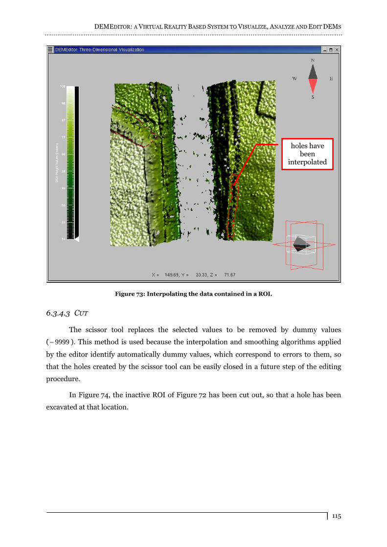
DEMEDITOR: A VIRTUAL REALITY BASED SYSTEM TO VISUALIZE, ANALYZE AND EDIT DEMS
115
Figure 73: Interpolating the data contained in a ROI.
6.3.4.3 CUT
The scissor tool replaces the selected values to be removed by dummy values
( 9999 ). This method is used because the interpolation and smoothing algorithms applied
by the editor identify automatically dummy values, which correspond to errors to them, so
that the holes created by the scissor tool can be easily closed in a future step of the editing
procedure.
In Figure 74, the inactive ROI of Figure 72 has been cut out, so that a hole has been
excavated at that location.
holes have
been
interpolated
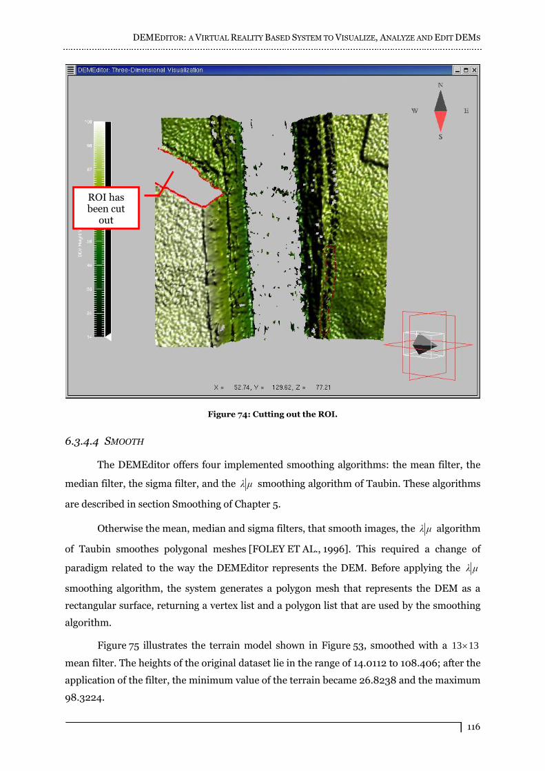
DEMEDITOR: A VIRTUAL REALITY BASED SYSTEM TO VISUALIZE, ANALYZE AND EDIT DEMS
116
Figure 74: Cutting out the ROI.
6.3.4.4 SMOOTH
The DEMEditor offers four implemented smoothing algorithms: the mean filter, the
median filter, the sigma filter, and the ìë smoothing algorithm of Taubin. These algorithms
are described in section Smoothing of Chapter 5.
Otherwise the mean, median and sigma filters, that smooth images, the ìë algorithm
of Taubin smoothes polygonal meshes [FOLEY ET AL., 1996]. This required a change of
paradigm related to the way the DEMEditor represents the DEM. Before applying the ìë
smoothing algorithm, the system generates a polygon mesh that represents the DEM as a
rectangular surface, returning a vertex list and a polygon list that are used by the smoothing
algorithm.
Figure 75 illustrates the terrain model shown in Figure 53, smoothed with a 1313
mean filter. The heights of the original dataset lie in the range of 14.0112 to 108.406; after the
application of the filter, the minimum value of the terrain became 26.8238 and the maximum
98.3224.
ROI has
been cut
out

DEMEDITOR: A VIRTUAL REALITY BASED SYSTEM TO VISUALIZE, ANALYZE AND EDIT DEMS
117
Figure 75: The virtual DEM smoothed with a mean filter.
6.3.4.5 DEFINITION OF MINIMUM AND MAXIMUM HEIGHT VALUES
In the 3D interface, the modification of the minimum and/or maximum height value
of the DEM can be done typing the new value in a command-line based widget or moving a
slider to the new desired height value (Figure 76), or manipulating the color-height palette
(Figure 59).
By changing the height value of the terrain through these options, they are only
removed visually. In order to remove the height values from the terrain, the cut tool has to be
executed, so that values less than (minimum modification) the minimum value specified by
the user are set to 9999 , and if there exist height values in the DEM array greater than
(maximum modification) the maximum value specified by the user, these values are also set
to 9999 .
Figure 76a illustrates a portion of a DEM with minimum height value 15.4586. Using
the widget interface, this value has been modified to 55.2528, what can be observed in the
new drawn DEM of Figure 76b.

DEMEDITOR: A VIRTUAL REALITY BASED SYSTEM TO VISUALIZE, ANALYZE AND EDIT DEMS
118
a b
Figure 76: Modifying the minimum height value of the DEM: a) before; b) after.
6.4 IMPLEMENTATION ISSUES
Some relevant implementation issues have been taken into account for the
development of the VR based system. An insight into each topic is given next.
6.4.1 A HIGH-RESOLUTION VIRTUAL ENVIRONMENT
Precise representation of data was a fundamental requirement for the successful use
of the DEMEditor, since without the adequate support for validation and editing procedures
it has no legality. Each pair of coordinates ),( yx and its corresponding z value had to be
represented accurately in order to construct a reliable 3D model of the DEM (see
section Concepts of Digital Elevation Models). Since airborne InSAR-based data can be of
very high-resolution (e.g., Orbisat da Amazônia S.A. [ORBISAT, 2004] released recently
OrbiSAR-1, an airborne InSAR sensor that achieves spatial resolution of 25 cm), the virtual
DEM should also be a high-resolution model, with high level of details (LOD) about the
imaged terrain.
6.4.2 PERFORMANCE
Traditionally, remote sensing users have to manipulate large amounts of data. A
system that intends to present lots of data for manipulation has to achieve this in a way that
allows the user to perform his/her tasks in a satisfactory manner.
Users of the DEMEditor should be able to explore DEMs stored in files with several
megabytes, perform analysis of the data and editing them. Consequently, performance was a
critical point in the implementation of the system.
In order to satisfy performance levels, the user may generate 3D DEM objects of
maximal 200200 pixels. This requirement was identified based on experiences with expert
DEMEDITOR: A VIRTUAL REALITY BASED SYSTEM TO VISUALIZE, ANALYZE AND EDIT DEMS
119
users, which had to perform exploration and editing tasks on real DEM data.
6.4.3 REALISM
Realism or impression of reality leads the user into a state commonly referred to as
immersion, or the suspension of disbelief. In the case presented here, representing precisely
the DEM as a 3D surface object, and offering the user resources to enhance reliability of the
virtual DEM made it possible to accomplish realism. In other words, the DEMEditor offers
the following functionalities:
to wrap the surface with an amplitude image of the terrain that matches precisely the
region represented in 3D;
to present elevation differences in the terrain through different levels of colors (for
example, dark colors represent lower areas, and bright colors represent higher areas);
to construct a compound representation through the presentation of contour levels
mapped over the surface model.
Whether to use or not these resources can be seen as a function of the LOD selected to
present the virtual world, which increases or decreases the realism of the environment and
supports data interpretation.
It is important to observe that a virtual environment, in order to be considered
realistic, does not need to present real-world objects exactly as they are in real life. A realistic
virtual environment is one where the user visualizes and interacts with the objects believing
them, and becomes involved with the environment.
6.4.4 INTERACTION IN THE VIRTUAL ENVIRONMENT
Interaction is one of the major advantages of VR interfaces, and a powerful tool for
exploring large sets of data. The DEMEditor contains some interaction tools that can be
exploited by specialist SAR data users without knowledge of how exploring DEMs in the 3D
space; this is a requirement in our system.
The DEMEditor implements simple, but powerful interaction techniques, that can be
used intuitively for manipulation of the virtual 3D DEM and for navigation through the
environment.
6.4.4.1 NAVIGATION STRATEGIES
Predefined walk-through tours to explore the virtual environment take the user to
places of interest for understanding the world. For example, an overview tour may show the
whole environment from a high position and help the user to obtain knowledge about the

DEMEDITOR: A VIRTUAL REALITY BASED SYSTEM TO VISUALIZE, ANALYZE AND EDIT DEMS
120
data. Another one would be a tour that takes the user to the four corners (south, north, east,
west) of the virtual 3D DEM. These tours allow the user to investigate the environment in an
easy way, since he/she is positioned and oriented during travel while obtaining constantly the
best angular view from each position.
Viewpoint navigation is a technique that allows the user to jump from one position in
the environment to another one, so that he/she obtains diverse impressions about the terrain
from different perspectives; each viewpoint is composed of a position and an orientation.
There are predefined viewpoints available for selection, and moreover these points of view,
the user can define his/her own viewpoints by creating new ones.
Free navigation through the virtual environment (walk tool of VRML plug-
ins [FRERY ET AL., 1999]), using the mouse, allows the user to explore the data without any
help from the system, what is sometimes desirable.
A compass icon has been introduced in the virtual environment to orient the user
about what direction to follow when he/she wants, for example, to go to a particular location.
Remote sensing users frequently use support material, such as maps, when performing
validation tasks on the data, so that an orientation tool may help them remain oriented
(avoid being overwhelmed) between all information sources.
6.4.4.2 OBJECT MANIPULATION
The user can select the virtual 3D DEM by pointing a mouse to it (study tool of
VRML plug-ins [FRERY ET AL., 1999]). This functionality is very important in order to
manipulate the DEM object, since the user can deal with the surface as he/she is used to do
with 3D objects in the real world. Once selected, the object may be rotated in space while it is
examined.
During exploration or edition tasks, the user may switch on a light source, and direct
it to a specific area of interest that he/she needs to visualize more carefully. This kind of
interaction uses translation, scaling and rotation transformations to manipulate objects, as
well as selection.
6.4.4.3 INTERACTION ICONS
Some icons have been introduced into the environment to help the user to interact
with the DEM data.
A color-height palette icon shows elevation information about the active DEM, and
the user can modify the minimum and maximum height values of the model by moving the
indicator to the new desired value.
DEMEDITOR: A VIRTUAL REALITY BASED SYSTEM TO VISUALIZE, ANALYZE AND EDIT DEMS
121
6.5 FINAL REMARKS
The DEMEditor has been developed in order to validate the methodology proposed by
this thesis, whose intention is to correct elevation errors in DEMs. However, another editing
tasks may also be performed using the system. For instance, if the terrain model is a digital
surface model that represents the objects over the terrain surface, it can be edited in order to
transform it in a digital ground model that represents the ground height information for that
terrain. On the other hand, a digital ground model could be populated with trees, roads,
houses, to name only a few, in order to create the digital surface model of a specific terrain. In
this case, a library containing 3D icons representing the objects to be used to modeling the
surface model would be required by the DEMEditor.
The DEMEditor has already been exhaustively tested, and also introduced to the VR
and remote sensing communities. Some works that focus on an overview of the
system [TEICHRIEB ET AL., 2002a; TEICHRIEB ET AL., 2002b; TEICHRIEB & KELNER,
2003], a detailed explanation of the editing module of the
DEMEditor [TEICHRIEB ET AL., 2003] and a description of a case study developed with the
editor [TEICHRIEB & KELNER, 2004] have been published.
CHAPTER 7
CASE STUDY
7.1 INTRODUCTION TO THE CHAPTER
After specifying the methodology proposed by this thesis to correct elevation errors in
DEMs and describing the implementation of this methodology through the development of
the DEMEditor, this chapter describes the system using real-world DEM data in order to
demonstrate how it may be utilized by the user to achieve his/her objectives.
Firstly, a brief introduction about the DEM used to perform the case study is given.
During the case study four tasks will be performed: DEM visualization, interaction with the
data, navigation through the virtual environment in order to explore it and, finally, editing of
errors found in the DEM.
At the end of the chapter a discussion is presented about the effectiveness of the
DEMEditor with respect to the application area.
7.2 DATA DESCRIPTION
This research work tackles data collected by an InSAR sensor, residing on an airborne
platform, and processed by a SAR and an interferometric processor. DEMs generated from
raw data collected by the AeS-1 [SCHWÄBISCH & MOREIRA, 1999] InSAR sensor,
developed by the company Aero-Sensing Radarsysteme GmbH, and processed by a
processing chain [WIMMER ET AL., 2000] based on InSAR technology have a total height
error of approximately 5 cm, when the imaged area has a flat topography with height
variations less than 5 m and is free of vegetation. With other types of land coverage and
topography the height accuracy remains of the order of 15 to 25 cm. DEMs with such levels of
accuracy are categorized as high precise elevation models.
The DEM used to present the case study described next has been collected in
Maastricht, Belgium, and has been supplied by Aero-Sensing Radarsysteme GmbH.
7.3 CASE STUDY
In the next subsections a case study is described, in which visualization, interaction,
exploration, analysis and editing are realized with the DEMEditor. Each topic is discussed
and illustrated, using the real-world dataset collected from the region of Maastricht.

CASE STUDY
123
7.3.1 REALISTIC DIGITAL ELEVATION MODEL VISUALIZATION
Figure 77 illustrates two ways to visualize DEM data: as a 2D image, and as a 3D
surface presented in a virtual environment. Indeed, the VR interface brings realism to the
presentation.
Figure 77b shows the DEM as a 3D surface wrapped with its corresponding grayscale
amplitude image, so that the user obtains a realistic impression about the shape of the
terrain, and also about how it looks when visualized in the real world. The 3D surface has
been positioned in the environment exactly in the same orientation as it appears in the 2D
image; this allows observing that the bright points presented as a diagonal line in Figure 77a
are spikes in the terrain, and that the dark area on the lower part of the image is the lowest
region of the terrain, which also contains some spikes.
a
b
Figure 77: Visualizing a DEM: a) 2D grayscale image; b) 3D surface object.
a
b
Figure 78: Enhancing realism and comprehension: a) colors; b) compound view.
Other ways to enhance realism of the virtual DEM are illustrated in Figure 78. In this
figure the vertices of the 3D surface are colored according to an elected color table to

CASE STUDY
124
highlight height variations in the terrain. The presented example shows the lowest areas in
blue and the highest as yellow colored areas. A smooth degrade between blue and yellow is
applied on the areas with intermediary height values. In Figure 78b the DEM is represented
as contour levels, combined with the 3D solid surface model, constituting a compound view
of the DEM in the virtual environment.
7.3.2 USER X DIGITAL ELEVATION MODEL: INTUITIVE AND EFFECTIVE
INTERACTION
Figure 79a shows a DEM with elevations between 86.94 and 108.37 m. The highest
values appear as bright areas on the surface whereas the lowest areas appear dark. The user
may modify these two values changing the height indicator, available on the bar on the left
side of the virtual environment, to a new desired minimum and/or maximum value. This
interactive way to edit the surface is especially useful if the user does not know exactly which
should be the new minimum/maximum values for the terrain. In this case, he/she can move
the height indicator until the DEM appears as desired. Figure 79b shows the same surface
with a maximum value modified to 100.00 m, obtained by moving the height indicator in the
virtual environment.
a
b
Figure 79: Interactive editing: a) original DEM; b) DEM with lower maximum value.
7.3.3 DIGITAL ELEVATION MODEL EXPLORATION THROUGH NAVIGATION
The imaging of a specific place using an airborne as a platform for the sensor allows
the people that perform field work to become important spatial knowledge about the terrain;
they can observe where are the highest areas that will be imaged, what vegetation cover is
present in the area, and possible reflection objects that could provoke spikes in the processed
DEM. The user can observe exactly the same things when he/she navigates through a virtual
environment to explore the 3D DEM.
Figure 78b shows an overview of a DEM. The user can see the whole terrain from this
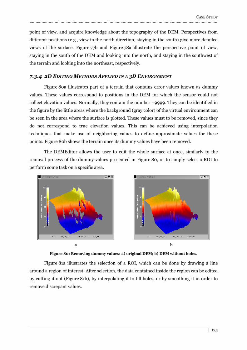
CASE STUDY
125
point of view, and acquire knowledge about the topography of the DEM. Perspectives from
different positions (e.g., view in the north direction, staying in the south) give more detailed
views of the surface. Figure 77b and Figure 78a illustrate the perspective point of view,
staying in the south of the DEM and looking into the north, and staying in the southwest of
the terrain and looking into the northeast, respectively.
7.3.4 2D EDITING METHODS APPLIED IN A 3D ENVIRONMENT
Figure 80a illustrates part of a terrain that contains error values known as dummy
values. These values correspond to positions in the DEM for which the sensor could not
collect elevation values. Normally, they contain the number �9999. They can be identified in
the figure by the little areas where the background (gray color) of the virtual environment can
be seen in the area where the surface is plotted. These values must to be removed, since they
do not correspond to true elevation values. This can be achieved using interpolation
techniques that make use of neighboring values to define approximate values for these
points. Figure 80b shows the terrain once its dummy values have been removed.
The DEMEditor allows the user to edit the whole surface at once, similarly to the
removal process of the dummy values presented in Figure 80, or to simply select a ROI to
perform some task on a specific area.
a
b
Figure 80: Removing dummy values: a) original DEM; b) DEM without holes.
Figure 81a illustrates the selection of a ROI, which can be done by drawing a line
around a region of interest. After selection, the data contained inside the region can be edited
by cutting it out (Figure 81b), by interpolating it to fill holes, or by smoothing it in order to
remove discrepant values.
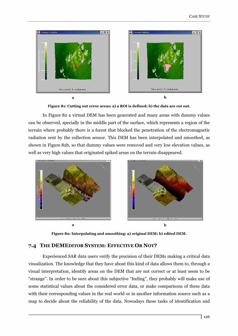
CASE STUDY
126
a
b
Figure 81: Cutting out error areas: a) a ROI is defined; b) the data are cut out.
In Figure 82 a virtual DEM has been generated and many areas with dummy values
can be observed, specially in the middle part of the surface, which represents a region of the
terrain where probably there is a forest that blocked the penetration of the electromagnetic
radiation sent by the collection sensor. This DEM has been interpolated and smoothed, as
shown in Figure 82b, so that dummy values were removed and very low elevation values, as
well as very high values that originated spiked areas on the terrain disappeared.
a
b
Figure 82: Interpolating and smoothing: a) original DEM; b) edited DEM.
7.4 THE DEMEDITOR SYSTEM: EFFECTIVE OR NOT?
Experienced SAR data users verify the precision of their DEMs making a critical data
visualization. The knowledge that they have about this kind of data allows them to, through a
visual interpretation, identify areas on the DEM that are not correct or at least seem to be
�strange�. In order to be sure about this subjective �feeling�, they probably will make use of
some statistical values about the considered error data, or make comparisons of these data
with their corresponding values in the real world or in another information source such as a
map to decide about the reliability of the data. Nowadays these tasks of identification and

CASE STUDY
127
verification of errors in DEMs are normally realized using systems based on 2D interfaces.
Examples of such systems are IDL and ENVI.
Although these environments are powerful tools for data visualization and analysis,
the task of making adjustments to DEMs with 2D interfaces is more intuitive and easy when
the third dimension is made available to the user through the use of a 3D interface. Figure 77
confirms the fact that DEMs may be much better visually interpreted when visualized with
3D interfaces, such as it is also done in the DEMEditor. Moreover that 3D interfaces enhance
realism of visualization, features pointed during the realization of analyses may be more
easily understood when seeing data as a 3D terrain.
The DEMEditor is a system based on VR interfaces. VR interfaces are essentially
interactive, since the user should be able to interfere with the stuff that happens in the
environment, and vice-versa. In spite of the fact that the DEMEditor uses a default flat
computer display instead of special immersion devices, which compromises the sensation of
being immersed in the virtual world as well as the level of user involvement with the
environment, it offers to the user the possibility to highly interact with the virtual DEM.
Interaction functionalities usually are poorly implemented or even do not exist in 2D
interfaces, and become important tools for performing exploration of large amounts of data
in order to seek for error areas in the DEM.
A point that certainly makes the DEMEditor an efficient system for correcting errors
in DEMs is that it makes possible visualize, explore, analyze and edit a DEM within the same
environment, through a 3D interface, and also a 2D one. This combination of functions
makes the DEMEditor a professional tool for the remote sensing community.
The DEMEditor supports DEM data with a raster format. In order to allow the
manipulation of other types of data, their file formats must be added to the system.
The DEMEditor has been developed for expert remote sensing users. If this is not the
case, the identification of errors in the DEM will be practically impossible with a system such
as the DEMEditor, since a user without knowledge about SAR data has not the ability to
interpret visually such data in order to identify anomalies. In this case, algorithms to identify
automatically error areas should be incorporated to the system. This can be accomplished
selecting adequate different methods already suggested in the literature (see Final Remarks
in Chapter 3) to be implemented in the editor, so that different kinds of errors can be
automatically identified. Another way to add automatic identification functionalities to the
DEMEditor is developing a new method able to identify different kinds of errors by specifying
characteristics of different errors to be identified and, based on this specification, build an
algorithm that is able to detect these errors; several studies have shown the difficulty to
accomplish such an objective.

CASE STUDY
128
7.5 FINAL REMARKS
The case study presented in this chapter shows that the DEMEditor may be used to
perform realistic visualization of DEMs, mainly due to the fact that data are presented as a
3D surface. Moreover, compound views may be constructed adding to the surface a model of
the contour levels of the surface, or elevation variations may be highlighted through the
association of colors to the surface vertices, or even a texture (for instance, the amplitude
picture corresponding to the DEM area) may be mapped to the surface enhancing its
appearance.
Interaction with the virtual data is another important functionality of the DEMEditor.
Basic navigation modes like walk and pan are available to explore the whole environment. In
order to manipulate 3D icons, the user may use rotation, translation and scaling
transformations, so that predefined actions are executed.
Analysis functions are available in the DEMEditor, which can be used during
exploration of the data in order to verify the precision of the DEM.
The editing functions of the DEMEditor become very relevant since the final objective
of the system is to correct errors in DEMs. The case study has presented some of these
functions, as they are used to enhance the accuracy of the terrain model.
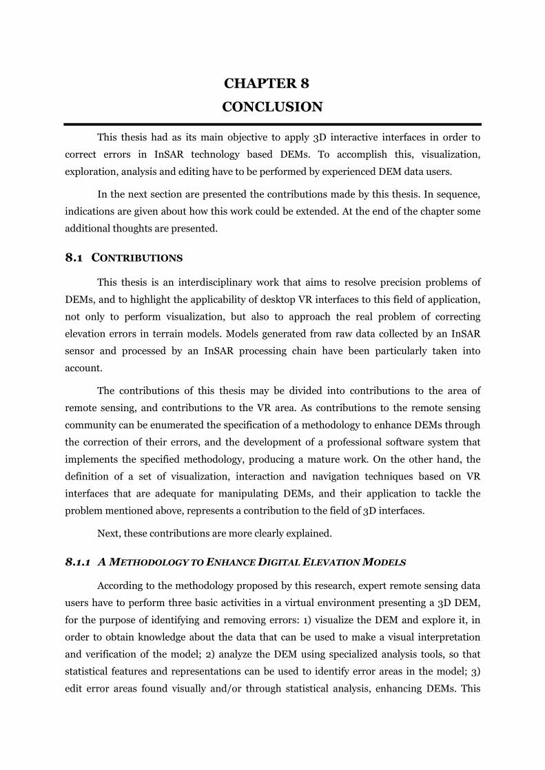
CHAPTER 8
CONCLUSION
This thesis had as its main objective to apply 3D interactive interfaces in order to
correct errors in InSAR technology based DEMs. To accomplish this, visualization,
exploration, analysis and editing have to be performed by experienced DEM data users.
In the next section are presented the contributions made by this thesis. In sequence,
indications are given about how this work could be extended. At the end of the chapter some
additional thoughts are presented.
8.1 CONTRIBUTIONS
This thesis is an interdisciplinary work that aims to resolve precision problems of
DEMs, and to highlight the applicability of desktop VR interfaces to this field of application,
not only to perform visualization, but also to approach the real problem of correcting
elevation errors in terrain models. Models generated from raw data collected by an InSAR
sensor and processed by an InSAR processing chain have been particularly taken into
account.
The contributions of this thesis may be divided into contributions to the area of
remote sensing, and contributions to the VR area. As contributions to the remote sensing
community can be enumerated the specification of a methodology to enhance DEMs through
the correction of their errors, and the development of a professional software system that
implements the specified methodology, producing a mature work. On the other hand, the
definition of a set of visualization, interaction and navigation techniques based on VR
interfaces that are adequate for manipulating DEMs, and their application to tackle the
problem mentioned above, represents a contribution to the field of 3D interfaces.
Next, these contributions are more clearly explained.
8.1.1 A METHODOLOGY TO ENHANCE DIGITAL ELEVATION MODELS
According to the methodology proposed by this research, expert remote sensing data
users have to perform three basic activities in a virtual environment presenting a 3D DEM,
for the purpose of identifying and removing errors: 1) visualize the DEM and explore it, in
order to obtain knowledge about the data that can be used to make a visual interpretation
and verification of the model; 2) analyze the DEM using specialized analysis tools, so that
statistical features and representations can be used to identify error areas in the model; 3)
edit error areas found visually and/or through statistical analysis, enhancing DEMs. This

CONCLUSION
130
methodology has been explained in detail in Chapter 5, Virtual Reality Interfaces Applied to
Enhance Digital Elevation Models.
Initially, there are no well-established methodologies applied to DEM data to address
problems of correcting errors. Decision rules about managing the errors in the data are
defined by individual DEM users. In this way, the presented methodology is an attempt to
define a functional methodology.
It has been considered that experienced remote sensing data users will use this
methodology. In this way, the background of the users about the data is an important tool
applied by the methodology in the error identification process. This characteristic allows the
identification (and correction) of any types of error in the DEMs, contrary to methods that
automatically identify errors looking for specific characteristics on the data, being able to
identify some specific types of anomalies only.
8.1.2 THE DEMEDITOR SYSTEM
The DEMEditor is a system that implements the methodology proposed by this thesis.
It has been described in Chapter 6, DEMEditor: a Virtual Reality Based System to Visualize,
Analyze and Edit DEM.
The DEMEditor is used for visualizing, analyzing and editing DEMs. It is a desktop
VR based system, which reconstructs real-world terrain (or surface) in VR. The virtual
environment is meant to be a place where specialized SAR data users explore and analyze
their large amounts of data, validate them according to known quality parameters and make
corrections on the DEM. Although the methodology is based on a 3D interface to correct
errors, the DEMEditor offers, moreover the 3D one, a 2D interface to perform visualization,
analysis and editing. This approach makes the DEMEditor a sophisticated system, offering to
the user the 2D environment already known by the remote sensing community to manipulate
its data, and the 3D interface that brings realism and interaction.
It is an important contribution to the remote sensing community, since the already
implemented systems are very simple and do only offer functionality to identify and/or
quantify errors in DEMs (with the exception of the DM4DEM tool, mentioned in Chapter 3).
In fact, most methods proposed for performing identification, quantification and correction
of errors has not been implemented as a useable application.
Finally, another mentionable aspect is that many analysis and editing functionalities
implemented in the DEMEditor have been developed based on requirements of expert DEM
users. These tools have been re-implemented based on sophisticated commercial tools and
adapted to fulfill these requirements, or specified and developed from scratch. For example,
CONCLUSION
131
the histogram and profile tools with the purpose of validating DEMs, and the ìë smoothing
algorithm of Taubin [TAUBIN, 2000], which has not previously been applied to smooth DEM
data.
8.1.3 THREE-DIMENSIONAL INTERFACES
This thesis shows that expert remote sensing data users can effectively use desktop
VR interfaces to tackle the problem of errors in DEMs, that is to say enhance DEMs, solving a
relevant problem of the remote sensing application area. The definition of a set of
visualization, interaction and navigation techniques based on VR interfaces that are adequate
for manipulating DEMs, and their application, served to accomplish this.
Interfaces perform an important role in this work because visual interpretation is a
central aspect of the process of identifying and correcting errors in DEMs. Experienced
remote sensing data users own knowledge about the data to be corrected, and feeling about
which areas are strong candidates to be error areas.
The area of remote sensing is a very promising, but yet unexplored application area
for VR. Although VR interfaces have largely been applied to visualize terrain data, they are
rarely used to implement applications that tackle real problems of this area. VR technology
has lots of benefits to bring to the remote sensing community; some of them have been
approached by this thesis.
8.2 FUTURE WORKS
This research has raised many questions and opened ways for additional applications
of the methodology specified in it and of the developed system, which will be briefly
presented next. Some alternatives to enhance the work produced by this thesis are also
explained below.
8.2.1 IMMERSIVE VIRTUAL REALITY INTERFACES
The desktop VR interface applied by this thesis brings realism and interaction, when
compared to the 2D interfaces commonly used by the remote sensing community. It has been
chosen to use non-immersive VR technology because it can be used with common computers
without the need for special immersion devices, which have a very high cost. Indeed, the use
of immersive VR interfaces to edit a terrain model would greatly enhance the realism,
interactivity and efficiency of the process. The sense of presence of the user certainly would
increase a lot when being in an immersive virtual environment during visualization and
editing of a DEM. Some researchers [SONG ET AL., 2000; BOWMAN ET AL., 2002b] have
studied and proposed interaction techniques for immersive virtual environments, which

CONCLUSION
132
could be applied in this work.
8.2.2 EVALUATION OF INTERFACES AND INTERACTION TECHNIQUES
Interfaces should be usable and intuitive in order that users can perform adequately
their tasks. Therefore, the evaluation of interfaces in order to assess their usability is a
relevant aspect [THOMAS & MACREDIE, 2002]. Moreover, as interaction plays an
important role in the work presented by this thesis, the techniques used could also be
evaluated in order to verify their applicability to the
application [BOWMAN ET AL., 1998; BOWMAN, 1999; BOWMAN ET AL., 2002a]. A testbed
evaluation for the assessment of interaction techniques for virtual environments can be
found in [BOWMAN ET AL., 2001b].
8.2.3 AUTOMATIC ERROR IDENTIFICATION
The DEMEditor does not use specialized algorithms to identify errors in DEMs.
Experienced users of such data are able to make a visual interpretation of the data and, using
their feeling, identify possible error areas that can later be verified in order to confirm their
suspicion. On the other hand, the use of �intelligent� tools specialized on specific types of
errors to verify data could support the user, helping him/her in the process of finding errors
in DEMs.
8.2.4 REPRESENTATION OF DIGITAL ELEVATION MODEL ERRORS
An additional functionality that the DEMEditor could include is the generation of
error models that represent the errors found in the DEM. Some algorithms to represent the
errors identified in terrain models are available in the literature. This option can be seen as
an information source for the user about the quality of the DEM.
8.2.5 QUANTIFICATION OF DIGITAL ELEVATION MODEL ERRORS
The quantification of errors in a DEM may also be a functionality desired in a system
that is used to correct errors, as the DEMEditor. The community has already proposed some
algorithms, which could be associated to the software. As the representation, the
quantification of errors in DEMs allows the verification of the precision level of a dataset.
8.2.6 EDITING METHODS
The DEMEditor contains some necessary functions for editing the terrain models.
Several important research works have defined sophisticated editing methods, which support
a set of editing operations. One example is the work of Barret and
Cheney [BARRET & CHENEY, 2002], which uses the concept of TRAPS (Tobogganed

CONCLUSION
133
Regions of Accumulated Plateaus) to edit in the object level. This and other methods could be
implemented in the DEMEditor and applied to edit the DEMs, enhancing the editing
capabilities of the system.
8.2.7 COLLABORATIVE EDITING OF DIGITAL ELEVATION MODELS
The system implemented in this thesis is a stand-alone system that allows a unique
user to exploit the application. The migration of this system to the Internet, so that the virtual
DEM can be accessed online through a Web browser, for example, would allow data to be
available for many users at the same time. Moreover, if such users would be able to work
simultaneously on the terrain model, in a collaborative environment, exchanging in real time
information about the data and editing the DEM, the process of correcting the model could
be improved in efficiency and accuracy. Techniques to manipulate objects collaboratively in
immersive virtual environments can be found in [PINHO ET AL., 2002].
8.2.8 SCENE MODELING IN THE DEMEDITOR
Frequently the DEM is required to represent the height values of the ground of the
mapped terrain, as well as the height values of the objects that cover the terrain, such as
fences, trees, houses, among others. In this case, the sensor used to collect raw data has to
pursue the capability to work in the X-band and in the P-band, in order to penetrate deeper
and map ground heights. If the user has a DEM that contains height information about the
objects above the ground, the DEMEditor could be used to edit these objects and construct a
ground based DEM. On the other hand, if the DEM represents the ground of the terrain, the
user could populate this DEM according to information sources about the terrain (pictures,
maps) and construct a 3D scene from this model, transforming it in a ground-coverage based
DEM.
8.2.9 OTHER APPLICATION AREAS
This research work has been developed with the objective of proposing a methodology
based on 3D desktop VR interfaces to edit DEMs. This methodology has been implemented,
originating an editor that can be used to visualize, explore, analyze and edit DEMs. Although
this system has the original function of supporting the correction of errors in DEMs, it could
be used for another applications. For instance, the DEMEditor could be used in the field of
telecommunications, for designing and simulating the installation of communication
antennas in a specific region modeled by the system, and for scientific visualization, in order
to manipulate molecular structures.
CONCLUSION
134
8.3 CLOSING THOUGHTS
This thesis tackles the problem of errors in DEMs, which occur basically due to
anomalies in the collection and processing procedures. The first thought is: in order to
produce as precise as possible DEMs, why are not realized several mappings on the terrain
and, finally, an average of the results is taken to generate the DEM? Certainly, a more precise
DEM would be generated as supposedly would be possible when a unique map had been
performed!
The answer for this question can be summarized with three words: cost, time and
external influence. The costs of maintaining a platform (e.g., an airborne) carrying an
imaging sensor, as well as the on field team that receives the raw data and starts processing
tasks are very high and would increase the projects budget in a unviable way. It would be a
very time consuming procedure that also increases the costs of the project. Moreover, natural
environment influences, such as wetness and vegetation grow, change fast terrain�s
conditions. If the imaging process takes to much time between each mapping, data become
different for each mapping, and produce inconsistent datasets.
The second thought is a consideration about the DEMEditor. The DEMEditor is not a
GIS, which mixes a geographic information visualization tool with data base functionalities to
query the data. The DEMEditor is a system implemented to edit DEMs, as well as visualize,
explore and analyze these models.

REFERENCES
BIBLIOGRAPHY
[BAKER, 2000] BAKER, Polly. Visualization spaces. ACM SIGGRAPH Computer Graphics,
34(4):8-10, 2000.
[BARRET & CHENEY, 2002] BARRET, William A.; CHENEY, Alan S. Object-based image
editing. In: INTERNATIONAL CONFERENCE ON COMPUTER GRAPHICS AND
INTERACTIVE TECHNIQUES, 29., 2002, San Antonio, Texas, Proceedings� New York,
USA: ACM Press, 2002. p. 777-784.
[BEIER & NEELY, 1992] BEIER, Thaddeus; NEELY, Shawn. Feature-based image
metamorphosis. In: INTERNATIONAL CONFERENCE ON COMPUTER GRAPHICS AND
INTERACTIVE TECHNIQUES, 19., 1992, Chicago, Proceedings� New York, USA: ACM
Press, 1992. p. 35-42.
[BIERMANN ET AL., 2002] BIERMANN, Henning; MARTIN, Ioana; BERNARDINI, Fausto;
ZORIN, Denis. Cut-and-paste editing of multiresolution surfaces. In: INTERNATIONAL
CONFERENCE ON COMPUTER GRAPHICS AND INTERACTIVE TECHNIQUES, 29., 2002,
San Antonio, Texas, Proceedings� New York, USA: ACM Press, 2002. p. 312-321.
[BOOKSTEIN, 1989] BOOKSTEIN, Fred L. Principal warps: thin-plate splines and the
decomposition of deformations. IEEE Transactions on Pattern Analysis and Machine
Intelligence, 11(6):567-585, 1989.
[BOWMAN ET AL., 2001a] BOWMAN, Doug A.; KRUIJFF, Ernst; LAVIOLA JR., Joseph J.;
POUPYREV, Ivan. An introduction to 3-D user interface design. Presence, 10(1):96-108,
2001.
[BUSTOS & FRERY, 2004] BUSTOS, Oscar H.; FRERY, Alejandro C. Statistical Functions
and Procedures in IDL 5.6. Preprint submitted to Elsevier Science, 2003.
URL: http://www.mathpreprints.com, visited on January 2004.
[CCRS, 2004] Fundamentals of remote sensing. Available: Canada Centre for Remote
Sensing site (Nov. 9, 1998).
URL: http://www.ccrs.nrcan.gc.ca/ccrs/learn/tutorials/fundam/fundam_e.html, visited on
January 2004.
[CONCAR, 2004] Comissão Nacional de Cartografia. Available: Comissão Nacional de
Cartografia site. URL: http://www.concar.ibge.gov.br/, visited on January 2004.
[COVRE, 1997] COVRE, Marcos. Do balão ao satélite. Revista Fator GIS. Curitiba, n. 20,
REFERENCES
136
October 1997.
[DURAÑONA & LÓPEZ, 2000] DURAÑONA, Gonzalo; LÓPEZ, Carlos. DM4DEM: a GRASS-
compatible tool for blunder detection of DEM. In: INTERNATIONAL SYMPOSIUM ON
SPATIAL ACCURACY ASSESSMENT IN NATURAL RESOURCES AND ENVIRONMENTAL
SCIENCES, 4., 2000, De Rode Hoed, Amsterdam, The Netherlands, Proceedings�
Amsterdam, The Netherlands: Delft University Press, 2000.
[DURAÑONA & LÓPEZ, 2001] DURAÑONA, Gonzalo; LÓPEZ, Carlos. Outlier detection in
DEMs. GIM INTERNATIONAL, 15(1):46-47, 2001.
[EHLSCHLAEGER, 1998] EHLSCHLAEGER, Charles R. The stochastic simulation
approach: tools for representing spatial application uncertainty. Santa Barbara, USA:
University of California, 1998. Ph.D. Dissertation.
[ELDER & GOLDBERG, 2001] ELDER, James H.; GOLDBERG, Richard M. Image editing in
the contour domain. IEEE Transactions on Pattern Analysis and Machine Intelligence,
23(3):291-296, 2001.
[FLASAR, 2000] FLASAR, Jan. 3D interaction in virtual environment. In: CENTRAL
EUROPEAN SEMINAR ON COMPUTER GRAPHICS, 4., 2000, Budmerice, Austria,
Proceedings�
[FREEMAN, 2004] FREEMAN, Tony. What is imaging radar? Available: Tropical Rain
Forest Information Center at NASA�s Jet Propulsion Laboratory site.
URL: http://trfic.jpl.nasa.gov/GRFM/cdrom/africa/docs/html/imgv3.htm, visited on
January 2004.
[FRERY ET AL., 1999] FRERY, Alejandro C.; KELNER, Judith; PAULA, Gustavo E. de;
SIEBRA, Clauirton de A.; SILVA, Danielle R. D. da; TEICHRIEB, Veronica. Avaliação
comparativa de tecnologias de suporte à VRML. In: WORKSHOP BRASILEIRO DE
REALIDADE VIRTUAL, 2., 1999, Marília, São Paulo, Brazil, Proceedings... Marília, São
Paulo, Brazil: Sociedade Brasileira de Computação, 1999. p. 127-138.
[FRERY ET AL., 2002] FRERY, Alejandro C.; KELNER, Judith; MOREIRA, João;
TEICHRIEB, Veronica. User satisfaction through empathy and orientation in three-
dimensional worlds. CyberPsychology and Behavior, 5(5):451-459, 2002.
[HIBBARD, 2000] HIBBARD, Bill. Confessions of a visualization skeptic. ACM SIGGRAPH
Computer Graphics, 34(3):11-13, 2000.
[INPE, 2004] Tutorial de Geoprocessamento. Available: Instituto Nacional de Pesquisas
Espaciais site. URL: http://www.dpi.inpe.br/, visited on January 2004.
[KELNER ET AL., 2000] KELNER, Judith; FRERY, Alejandro C.; MOREIRA, João; PESSOA,
REFERENCES
137
Bárbara; ALHEIROS, Daniel; ARAÚJO FILHO, Mozart de S. C.; TEICHRIEB, Veronica.
Desktop virtual reality in the assessment of tidal effect. In: INTERNATIONAL GEOSCIENCE
AND REMOTE SENSING SYMPOSIUM, 20., 2000, Honolulu, Hawaii, USA, Proceedings�
Hawaii, USA: IEEE Press, 2000, v.1. p. 1-3.
[KELNER ET AL., 2001] KELNER, Judith; FRERY, Alejandro C.; TEICHRIEB, Veronica;
ARAÚJO FILHO, Mozart de S. C. Simulation and assessment of flooding with desktop virtual
reality. In: SYMPOSIUM ON VIRTUAL REALITY, 4., 2001, Florianópolis, Brazil,
Proceedings� Florianópolis, Brazil: Sociedade Brasileira de Computação, 2001. p. 56-66.
[LÓPEZ, 1997] LÓPEZ, Carlos. Locating some types of random errors in digital terrain
models. International Journal of Geographical Information Science, 11(7):677-689, 1997.
[LÓPEZ, 2000] LÓPEZ, Carlos. On the improving of elevation accuracy of digital elevation
models: a comparison of some error detection procedures. Transactions on GIS, 1(1):43-64,
2000.
[LUM & MA, 2002] LUM, Eric B.; MA, Kwan-Liu. Interactivity is the key to expressive
visualization. ACM SIGGRAPH Computer Graphics, 36(3): 5-9, 2002.
[LUM ET AL., 2002] LUM, Eric B.; STOMPEL, Aleksander; MA, Kwan Liu. Kinetic
visualization: a technique for illustrating 3D shape and structure. In: IEEE VISUALIZATION,
2002, Boston, Massachusetts, USA, Proceedings� Piscataway, USA: IEEE Press, 2002. p.
435-442.
[MAZURYK & GERVAUTZ, 1996] MAZURYK, Tomasz; GERVAUTZ, Michael. Virtual reality
history, applications, technology and future. Technical Report TR-186-2-96-06, 1996.
[MOREIRA, 1992] MOREIRA, João. Bewegungsextraktionsverfahren für radar mit
synthetischer apertur. Munich, Germany: DLR, 1992. 131p. Doktorarbeit.
[MORTENSEN, 2000] MORTENSEN, Eric N. Simultaneous multi-frame subpixel boundary
definition using toboggan-based intelligent scissors for image and movie editing. Provo, UT:
Department of Computer Science, Brigham Young University, 2000. 289p. Doctoral
Dissertation.
[MORTENSEN & BARRETT, 1998] MORTENSEN, Eric N.; BARRETT, William A.
Interactive segmentation with intelligent scissors. Graphical Models and Image Processing,
60(5):349-384, 1998.
[MORTENSEN & BARRETT, 1999] MORTENSEN, Eric N.; BARRETT, William A. Toboggan-
based intelligent scissors with a four parameter edge model. In: IEEE COMPUTER VISION
AND PATTERN RECOGNITION, 2., 1999, Fort Collins, CO, Proceedings� USA: IEEE Press,
1999. p. 452-458.

REFERENCES
138
[MORTENSEN ET AL., 2000] MORTENSEN, Eric N.; REESE, L. Jack; BARRETT, William
A. Intelligent selection tools. IEEE Computer Vision and Pattern Recognition, II:776-777,
2000.
[NASA EARTH OBSERVATORY, 2004] Earth Observatory. Available: NASA�s Earth
Observatory site. URL: http://earthobservatory.nasa.gov, visited on January 2004.
[NASA OBSERVATORIUM - History, 2004] Remote sensing in history. Available: NASA�s
Observatorium site.
URL: http://observe.arc.nasa.gov/nasa/exhibits/history/history_0.html, visited on January
2004.
[NASA OBSERVATORIUM - Resources, 2004] Remote sensing resources. Available: NASA�s
Observatorium site.
URL: http://observe.arc.nasa.gov/nasa/education/reference/main.html, visited on January
2004.
[NASA SIM, 2004] Interferometry. Available: NASA�s Space Interferometry Mission site.
URL: http://sim.jpl.nasa.gov/interferometry/index.html, visited on January 2004.
[ORBISAT, 2004] Orbisat Remote Sensing. Available: Orbisat da Amazônia S.A. site.
URL: http://www.orbisat.com.br/remote_sensing/index.html, visited on January 2004.
[REIGBER, 2001] REIGBER, Andreas. SAR interferometry: an introduction. Rennes:
Andreas Reigber, 2001. 46 transparencies, color.
[REIGBER, 2004] REIGBER, Andreas. Synthetic aperture radar � Basic concepts and image
formation. Available: Epsilon.Nought Radar Remote Sensing site.
URL: http://epsilon.nought.de/tutorials/processing/index.php, visited on January 2004.
[SCHWÄBISCH, 1995] SCHWÄBISCH, Marcus. Die SAR-Interferometrie zur erzeugung
digitaler geländemodelle. Stuttgart, Germany: Stuttgart University, 1995. 125p.
Doktorarbeit.
[SCHWÄBISCH & MOREIRA, 1999] SCHWÄBISCH, Marcus; MOREIRA, João. The high
resolution airborne interferometric SAR AeS-1. In: INTERNATIONAL AIRBORNE REMOTE
SENSING CONFERENCE AND CANADIAN SYMPOSIUM ON REMOTE SENSING, 4. and
21., 1999, Ottawa, Canada, Proceedings�
[SHORT, 2004] SHORT, Nicholas M. The remote sensing tutorial. Available: NASA site.
URL: http://rst.gsfc.nasa.gov/start.html, visited on January 2004.
[TAUBIN, 2000] TAUBIN, Gabriel. Geometric signal processing on polygonal meshes.
In: EUROGRAPHICS, 2000, Pasadena, USA, STAR � State of The Art Report� The
Eurographics Association, 2000.
REFERENCES
139
[TEICHRIEB, 1999] TEICHRIEB, Veronica. Avatares como Guias Interativos para Auxílio
na Navegação em Ambientes Virtuais Tridimensionais. Recife, Brazil: Centro de
Informática, Universidade Federal de Pernambuco, 1999. 148p. Dissertação de Mestrado.
[TEICHRIEB & KELNER, 2003] TEICHRIEB, Veronica; KELNER, Judith. Virtual reality
interfaces applied to correct elevation errors in digital elevation models. In: SYMPOSIUM
ON VIRTUAL REALITY, 6., 2003, Ribeirão Preto, Brazil, Proceedings� Ribeirão Preto,
Brazil: Brazilian Computer Society, 2003.
[TEICHRIEB & KELNER, 2004] TEICHRIEB, Veronica; KELNER, Judith. DEMEditor: a
virtual reality system to enhance the precision of digital elevation models. In: ASPRS, 2004,
Denver, USA, Proceedings� To be presented in May 2004.
[TEICHRIEB ET AL., 2002a] TEICHRIEB, Veronica; FRERY, Alejandro C.; KELNER,
Judith. DEMEditor: a tool for editing DEMs. In: INTERNATIONAL CONFERENCE IN
CENTRAL EUROPE ON COMPUTER GRAPHICS, VISUALIZATION AND COMPUTER
VISION, 10., 2002, Plzen, Czech Republic, Proceedings� Plzen, Czech Republic: INSPEC,
2002.
[TEICHRIEB ET AL., 2002b] TEICHRIEB, Veronica; KELNER, Judith; FRERY, Alejandro C.
Visualization, analysis and editing of digital elevation models. In: SYMPOSIUM ON
VIRTUAL REALITY, 5., 2002, Fortaleza, Brazil, Proceedings� Fortaleza, Brazil: Brazilian
Computer Society, 2002. p. 250�261.
[TEICHRIEB ET AL., 2003] TEICHRIEB, Veronica; KELNER, Judith; FRERY, Alejandro C.
Virtual reality interfaces applied to the editing of digital elevation models. In: SIMPÓSIO
BRASILEIRO DE SENSORIAMENTO REMOTO, 11., 2003, Belo Horizonte, Brazil, Anais�
São José dos Campos, Brazil: INPE (Instituto Nacional de Pesquisas Espaciais), 2003. p.
401�408. CD-ROM.
[USGS, 1997] Standards for digital elevation models, part 1: general, part 2: specifications,
part3: quality control. United States Department of the Interior, United States Geological
Survey (USGS), National Mapping Division, Washington, DC. 1997. National Mapping
Program, Technical Instructions.
[WECHSLER, 2000] WECHSLER, Suzanne P. Effect of DEM uncertainty on topographic
parameters, DEM scale and terrain evaluation. New York, USA: State University of New
York College of Environmental Science and Forestry, 2000. 380p. Ph.D. Thesis.
[WIMMER ET AL., 2000] WIMMER, Christian; SIEGMUND, Robert; SCHWÄBISCH,
Marcus; MOREIRA, João. Generation of high precision DEMs of the Wadden Sea with
airborne interferometric SAR. IEEE Transactions on Geoscience and Remote Sensing,
38(5):2234-2245, 2000.
REFERENCES
140
[WINGRAVE ET AL., 2002] WINGRAVE, Chadwick; BOWMAN, Doug A.;
RAMAKRISHNAN, Naren. Towards preferences in virtual environment interfaces.
In: EUROGRAPHICS WORKSHOP ON VIRTUAL ENVIRONMENTS, 8., 2002,
Proceedings� The Eurographics Association, 2002.
[WOOD, 1996] WOOD, Joseph. The geomorphological characterization of digital elevation
models. Leicester, UK: Department of Geography, University of Leicester, 1996. 185p. Ph.D.
Thesis.
[ZWICKER ET AL., 2002] ZWICKER, Matthias; PAULY, Mark; KNOLL, Oliver; GROSS,
Markus. Pointshop 3D: an interactive system for point-based surface editing. In:
INTERNATIONAL CONFERENCE ON COMPUTER GRAPHICS AND INTERACTIVE
TECHNIQUES, 29., 2002, San Antonio, Texas, Proceedings� New York, USA: ACM Press,
2002. p. 322-329.
ADDITIONAL REFERENCES
[ACEVEDO, 1991] ACEVEDO, W. First assessment of US Geological Survey 30-minute
DEM's: a great improvement over existing 1-degree data. ASPRS-ACSM - Technical Papers,
2:1-14, 1991.
[ADOBE, 2004] Adobe. Available: Adobe Systems Incorporated site.
URL: http://www.adobe.com, visited on January 2004.
[ADOBE PHOTOSHOP, 2004] Adobe Photoshop 7. Available: Adobe Systems Incorporated
site. URL: http://www.adobe.com/products/photoshop/main.html, visited on January 2004.
[AERO-SENSING, 2001] Aero-Sensing Radarsysteme. Available: Aero-Sensing
Radarsysteme GmbH site. URL: http://www.aerosensing.de/, visited on November 2001.
[AMES ET AL., 1997] AMES, Andrea L.; NADEAU, David R.; MORELAND, John L. VRML
2.0 Sourcebook. 2nd ed. New York, USA: Wiley, 1997.
[BAXES, 1994] BAXES, Gregory A. Digital image processing. Principles and applications.
New York: John Wiley & Sons, Inc., 1994. 452p.
[BOWMAN, 1999] BOWMAN, Doug A. Interaction techniques for common tasks in
immersive virtual environments. Design, evaluation, and application. Georgia, USA: Georgia
Institute of Technology, 1999. 142p. Doctoral dissertation.
[BOWMAN ET AL., 1998] BOWMAN, Doug A.; HODGES, Larry F.; BOLTER, Jay. The
virtual venue: user-computer interaction in information-rich virtual environments. Presence,
7(5):478-493, 1998.
[BOWMAN ET AL., 2001b] BOWMAN, Doug A.; JOHNSON, Donald B.; HODGES, Larry F.
REFERENCES
141
Testbed evaluation of virtual environment interaction techniques. Presence, 10(1):75-95,
2001.
[BOWMAN ET AL., 2002a] BOWMAN, Doug A.; GABBARD, Joseph L.; HIX, Deborah. A
survey of usability evaluation in virtual environments: classification and comparison of
methods. Presence, 11(4):404-424, 2002.
[BOWMAN ET AL., 2002b] BOWMAN, Doug A.; RHOTON, Christopher J.; PINHO, Márcio
S. Text input techniques for immersive virtual environments: an empirical comparison. In:
HUMAN FACTORS AND ERGONOMICS SOCIETY ANNUAL MEETING, 46., 2002,
Proceedings� p. 2154-2158.
[BRANDFASS ET AL., 2000] BRANDFASS, Michael; HOFMANN, Christoph; MURA, Jose
C.; PAPATHANASSIOU, Konstantinos P. Polarimetric SAR interferometry as applied to fully
polarimetric rain forest data. In: INTERNATIONAL GEOSCIENCE AND REMOTE SENSING
SYMPOSIUM, 20., 2000, Honolulu, Hawaii, USA, Proceedings� Hawaii, USA: IEEE Press,
2000.
[BROWN & BARA, 1994] BROWN, Daniel; BARA, Thaddeus. Recognition and reduction of
systematic error in elevation and derivative surfaces from 7.5-minute DEMs.
Photogrammetric Engineering and Remote Sensing, 60(2):189-194, 1994.
[BURDICK, 1997] BURDICK, Howard E. Digital imaging: theory and applications. New
York: McGraw-Hill, 1997. 315p.
[BURROUGH, 1986] BURROUGH, Peter. Principles of geographical information systems
for land resources assessment. New York: Oxford University Press, 1986. 194p.
[CLIFF & ORD, 1981] CLIFF, A. D.; ORD, J. K. Spatial processes, models and applications.
London: Pion, 1981.
[DEITEL & DEITEL, 1998] DEITEL, Harvey M.; DEITEL, Paul J. Java: how to program. 2nd
ed. New Jersey, USA: Prentice Hall, 1998.
[DESMET, 1997] DESMET, P. Effects of interpolation errors on the analysis of DEMs. Earth
Surface Processes and Landforms, 22:563-580, 1997.
[ENGLUND, 1993] ENGLUND, Evan. Spatial simulation: environmental applications.
In: ENVIRONMENTAL MODELING WITH GIS, Edited by Michael Goodchild, Bradley
Parks, Louis Steyaert. New York, NY: Oxford University Press, 1993. p. 432-446.
[ESRI, 1998] Environmental Systems Research Institute (ESRI). ArcView Spatial Analyst
Online User Guide. Redlands, California, 1998.
[FOLEY ET AL., 1996] FOLEY, James D.; VAN DAM, Andries; FEINER, Steven K.;
REFERENCES
142
HUGHES, John F. Computer graphics: principles and practice. Second edition in C. USA:
Addison-Wesley Publishing Company, 1996.
[GIMP, 2004] The GIMP. Available: GIMP site. URL: http:www.gimp.org, visited on January
2004.
[GOMES & VELHO, 1994] GOMES, Jonas; VELHO, Luiz. Computação gráfica: imagem. Rio
de Janeiro: IMPA e SBM, 1994. 424p. (Série de Computação e Matemática).
[GOMES & VELHO, 1998] GOMES, Jonas; VELHO, Luiz. Computação gráfica, volume 1.
Rio de Janeiro: IMPA, 1998. 323p. (Série de Computação e Matemática).
[GONZALEZ & WOODS, 2000] GONZALEZ, Rafael C.; WOODS, Richard E. Processamento
de imagens digitais. São Paulo: Editora Edgard Blücher Ltda., 2000. 509p.
[HUNTER & GOODCHILD, 1995] HUNTER, G.; GOODCHILD, M. Dealing with error in
spatial databases: a simple case study. Photogrammetric Engineering and Remote Sensing,
61(5):529-537, 1995.
[IDL, 1998] IDL objects and object graphics. Colorado: Research Systems, Inc., 1998. 380p.
[INTERMAP, 2004] Intermap Technologies. Available: Intermap Technologies Corp. site.
URL: http://www.intermaptechnologies.com/, visited on January 2004.
[JAIN, 1989] JAIN, Anil K. Fundamentals of digital image processing. Englewood Cliffs,
New Jersey: Prentice Hall, 1989. 569p.
[JRBP, 2004] Jasper Ridge Biological Preserve. Available: Stanford University site.
URL: http://jasper1.stanford.edu/research/sitedata/maps/contours.html, visited on January
2004.
[KENT & KENT, 1997] KENT, Peter; KENT, John. JavaScript para Netscape: guia oficial.
São Paulo, Brazil: Makron Books do Brasil, 1997. 437p.
[KITANIDIS, 1997] KITANIDIS, P. Introduction to geostatistics: applications in
hydrogeology. New York, NY: Cambridge University Press, 1997. 249p.
[LI, 1988] LI, Zhilin. On the measure of digital terrain model accuracy. Photogrammetric
Record, 12(72):873-877, 1988.
[MATHWORKS, 2004] The MathWorks. Available: The MathWorks, Inc. site.
URL: http://www.mathworks.com/, visited on January 2004.
[MONCKTON, 1994] MONCKTON, Colin. An investigation into the spatial structure of error
in digital elevation data. In: INNOVATIONS IN GIS, volume 1, Ed. Michael F. Worboys.
Bristol: Taylor and Francis, Inc., 1994. 267p.

REFERENCES
143
[OPENGL, 2004] OpenGL. Available: Silicon Graphics, Inc. site.
URL: http://www.opengl.org/, visited on January 2004.
[PINHO ET AL., 2002] PINHO, Márcio S.; BOWMAN, Doug A.; FREITAS, Carla M. D. S.
Cooperative object manipulation in immersive virtual environments: framework and
techniques. In: ACM VIRTUAL REALITY SOFTWARE TECHNOLOGY, 2002, Hong Kong,
Proceedings� New York, USA: ACM Press, 2002. p. 171-178.
[POLIDORI ET AL., 1991] POLIDORI, L.; CHOROWICZ, J.; GUILLANDE, R. Description of
terrain as a fractal surface and application to digital elevation model quality assessment.
Photogrammetric Engineering and Remote Sensing, 57(10):1329-1332, 1991.
[POUPYREV & KRUIJFF, 2004] POUPYREV, Ivan; KRUIJFF, Ernst. 20th century 3DUI
bibliography: annotated bibliography of 3D user interfaces of the 20th century.
Available: ATR Media Integration & Communications Research Laboratories site.
URL: http://www.mic.atr.co.jp/~poup/3dui/3duibib.htm, visited on January 2004.
[RESEARCH SYSTEMS, 2004] Research Systems. Available: Research Systems, Inc. site.
URL: http://www.rsinc.com/, visited on January 2004.
[ROBERTSON ET AL., 1997] ROBERTSON, George; CZERWINSKI, Mary; DANTZICH,
Maarten van. Immersion in desktop virtual reality. In: ACM SYMPOSIUM ON USER
INTERFACE SOFTWARE AND TECHNOLOGY, 10., 1997, Alberta, Canada, Proceedings�
New York, USA: ACM Press, 1997. p. 11-19.
[ROCKWOOD & CHAMBERS, 1996] ROCKWOOD, Alyn; CHAMBERS, Peter. Interactive
curves and surfaces: a multimedia tutorial on CAGD. San Francisco, California: Morgan
Kaufmann Publishers, Inc., 1996. 192p. (The Morgan Kaufmann Series in Computer Graphics
and Geometric Modeling). Series edited by Brian A. Barsky.
[RUBINSTEIN, 1981] RUBINSTEIN, Reuven Y. Simulation and the monte carlo method.
New York: John Willey and Sons, 1981.
[RUDDLE ET AL., 1998] RUDDLE, Roy A.; PAYNE, Stephen J.; JONES, Dylan M.
Navigating large-scale �desktop� virtual buildings: effects of orientation aids and familiarity.
Presence, 7(2):179-192, 1998.
[SABINS, 1987] SABINS, F. F. Remote sensing principles and interpretation. 2nd ed. W. H.
Freeman & Co., 1987. 449p.
[SONG ET AL., 2000] SONG, Chang Geun; KWAK, No Jun; JEONG, Dong Hyun. Developing
an efficient technique of selection and manipulation in immersive V.E. In: ACM VIRTUAL
REALITY SOFTWARE TECHNOLOGY, 2000, Seoul, Korea, Proceedings� New York, USA:
ACM Press, 2000. p. 142-146.

REFERENCES
144
[SPEAR ET AL., 1996] SPEAR, Morwenna; HALL, Jane; WADSWORTH, Richard.
Communication of uncertainty in spatial data to policy makers. In: INTERNATIONAL
SYMPOSIUM ON SPATIAL ACCURACY ASSESSMENT IN NATURAL RESOURCES AND
ENVIRONMENTAL SCIENCES, 2., Fort Collins, Colorado, USA, Report RM-GTR-277�
1996. p. 199-207.
[TAYLOR, 1997] TAYLOR, John. An introduction to error analysis: the study of
uncertainties in physical measurements. Sausalito, CA: University Science Books, 1997.
327p.
[THEOBALD, 1989] THEOBALD, David. Accuracy and bias issues in surface representation.
In: THE ACCURACY OF SPATIAL DATABASES, Eds. Michael F. Goodchild and Sucharita
Gopal. Bristol: Taylor and Francis, Inc., 1989. p. 99-106.
[THOMAS & MACREDIE, 2002] THOMAS, Peter; MACREDIE, Robert D. Introduction to
the new usability. ACM Transactions on Computer-Human Interaction, 9(2):69-73, 2002.
[VRML, 2004] The Virtual Reality Modeling Language. Available: Web 3D Consortium site
(1999). URL: http://www.web3d.org/technicalinfo/specifications/ISO_IEC_14772-
All/index.html, visited on January 2004.
[WISE, 1998] WISE, Stephen. The effect of GIS interpolation errors on the use of digital
elevation models in geomorphology. Edited by S. N. Lane, K. S. Richards and J. H. Chandler,
John Wiley and Sons, 1998. 300p.
[WOOD & FISHER, 1993] WOOD, J.; FISHER, P. Assessing interpolation accuracy in
elevation models. IEEE Computer Graphics and Applications, 13(2):48-56, 1993.

APPENDIX
CLASS DIAGRAM
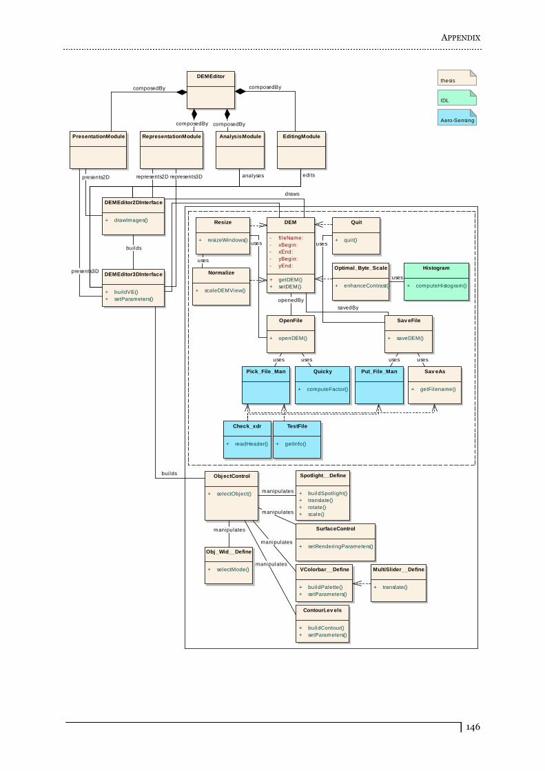
APPENDIX
146
DEMEditor
DEMEditor2DInterface
+ drawImages()
DEMEditor3DInterface
+ bui ldVE()+ setParameters()
Aero-Sensing
IDL
thesis
PresentationModule RepresentationModule AnalysisModule EditingModule
DEM
- fi leName: - xBegin: - xEnd: - yBegin: - yEnd:
+ getDEM()+ setDEM()
Quit
+ quit()
Pick_File_Man
Resize
+ resizeWindows()
Check_xdr
+ readHeader()
TestFile
+ getInfo()
Normalize
+ scaleDEMView()
OpenFile
+ openDEM()
Quicky
+ computeFactor()
Put_File_Man Sav eAs
+ getFi lename()
Sav eFile
+ saveDEM()
Optimal_Byte_Scale
+ enhanceContrast()
Histogram
+ computeHistogram()
VColorbar__Define
+ buildPalette()+ setParameters()
MultiSlider__Define
+ translate()
ObjectControl
+ selectObject()
Obj_Wid__Define
+ selectMode()
SurfaceControl
+ setRenderingParameters()
Spotlight__Define
+ buildSpotlight()+ translate()+ rotate()+ scale()
ContourLev els
+ buildContour()+ setParameters()
uses
openedBy
uses
uses
savedBy
usesuses
builds
uses
usesuses
presents3D
manipulates
composedBy
composedBycomposedBy
composedBy
represents3D
builds
manipulates
presents2D
draws
manipulates
manipulates
manipulates
editsanalysesrepresents2D
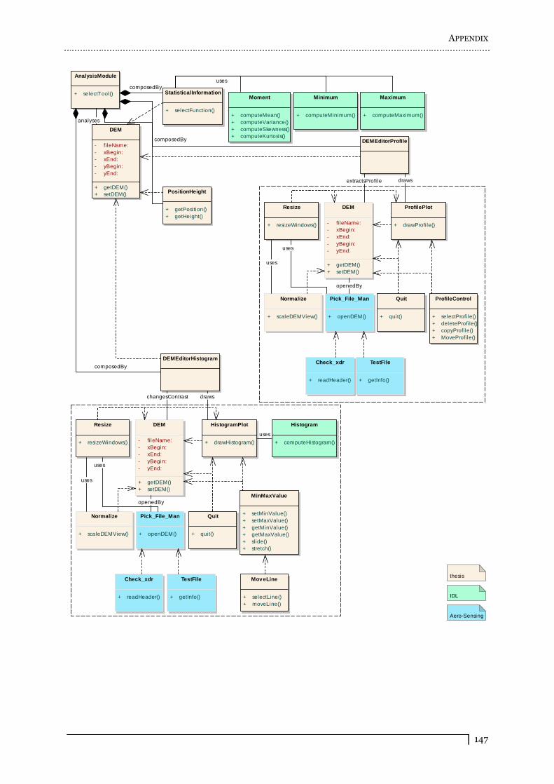
APPENDIX
147
MoveLine
+ selectLine()+ moveLine()
Normalize
+ scaleDEMView()
MinMaxValue
+ setMinValue()+ setMaxValue()+ getMinValue()+ getMaxValue()+ sl ide()+ stretch()
Histogram
+ computeHistogram()
TestFile
+ getInfo()
Check_xdr
+ readHeader()
Resize
+ resizeWindows()
Pick_File_Man
+ openDEM()
Quit
+ quit()
HistogramPlot
+ drawHistogram()
DEM
- fileName: - xBegin: - xEnd: - yBegin: - yEnd:
+ getDEM()+ setDEM()
DEM
- fileName: - xBegin: - xEnd: - yBegin: - yEnd:
+ getDEM()+ setDEM()
DEMEditorHistogram
StatisticalInformation
+ selectFunction()
PositionHeight
+ getPosition()+ getHeight()
DEMEditorProfile
DEM
- fileName: - xBegin: - xEnd: - yBegin: - yEnd:
+ getDEM()+ setDEM()
ProfilePlot
+ drawProfi le()
Quit
+ quit()
Resize
+ resizeWindows()
Check_xdr
+ readHeader()
TestFile
+ getInfo()
Normalize
+ scaleDEMView()
ProfileControl
+ selectProfile()+ deleteProfi le()+ copyProfile()+ MoveProfile()
Moment
+ computeMean()+ computeVariance()+ computeSkewness()+ computeKurtosis()
Minimum
+ computeMinimum()
Maximum
+ computeMaximum()
AnalysisModule
+ selectTool()
Pick_File_Man
+ openDEM()
Aero-Sensing
IDL
thesis
extractsProfi le draws
changesContrast
uses
openedBy
uses
uses
composedBy
uses
composedBy
composedBy
uses
uses
openedBy
analyses
draws

APPENDIX
148
DEM
- fi leName: - xBegin: - xEnd: - yBegin: - yEnd:
+ getDEM()+ setDEM()
ROI
+ drawROI()+ selectROI()+ deleteROI()+ getROI()
Interpolation
+ selectInterpolation()+ getROIPoints()+ countDummy()
Smooth
+ getParameter()+ selectFi lter()+ getROIPoints()
Cut
+ getROIPoints()+ cut()
MinMax
+ getMin()+ getMax()+ setMin()+ setMax()
bilinearInterpolation
+ interpolate()
meanInterpolation
+ interpolate()
meanFilter
+ smooth()
medianFilter
+ smooth()
sigmaFilter
+ smooth()
taubinAlgorithm
+ smooth()
EditingModule
+ selectTool()+ undo()+ update()
Aero-Sensing
IDL
thesis
uses
composedBy
composedBy
edits
uses
uses
uses
composedBycomposedBy
composedBy
uses
uses