designing collective decision-making dynamics for multi
TRANSCRIPT
Designing collective decision-making
dynamics for multi-agent systems
with inspiration from honeybees
Rebecca A.L. Gray
A Dissertation
Presented to the Faculty
of Princeton University
in Candidacy for the Degree
of Doctor of Philosophy
Recommended for Acceptance
by the Department of
Mechanical and Aerospace Engineering
Adviser: Naomi Ehrich Leonard
September 2019

c© Copyright by Rebecca A.L. Gray, 2019.
All rights reserved.
Abstract
For many multi-agent systems, collective decision-making among alternatives is a
crucial task. A group of agents may be required to collectively decide on their next
action, and may face limitations on their sensing, communication and computational
abilities. A swarm of honeybees choosing a new nest-site faces these challenges, and
has been shown to reliably make decisions with accuracy, efficiency and adaptability.
The honeybee decision-making dynamics can be modelled by a pitchfork bifurcation,
a nonlinear phenomenon that is ubiquitous in animal decision-making.
We describe and analyse a model for collective decision-making that possesses
a pitchfork bifurcation. The model allows us to leverage the characteristics of the
honeybee dynamics for application in multi-agent network systems and to extend the
capabilities of our decision-making dynamics beyond those of the biological system.
Using tools from nonlinear analysis, we show that our model retains some impor-
tant characteristics of the honeybee decision-making dynamics, and we examine the
impact of system and environmental parameters on the behaviour of the model. We
derive an extension to an existing centrality measure to describe the relative influence
of each agent, and to show how agent preferences can lead to bias in the network.
We design decentralised, adaptive feedback dynamics on a parameter of the model,
which ensure that a decision is made. We discuss how this system parameter, which
quantifies how much each agent is influenced by its neighbours, provides an intuitive
mechanism to involve a human operator in the decision-making. We continue this
discussion as we implement our model with a simple robotic system.
Throughout this thesis, we discuss the trade-off in the design of decision-making
dynamics between systems that are robust to unwanted disturbances, but are also
sensitive to the values of important system parameters. We show how dynamics
modelled by a pitchfork bifurcation exhibit hypersensitivity close to the bifurcation
point, and hyperrobustness far away from it.
iii

Acknowledgements
Before moving to USA to begin graduate schooling I had several conversations with
my father about his graduate school experience in the USA, and what he had enjoyed
about it. In particular I remember him saying that he loved the enthusiasm of the
people about the work they were doing, and the positive research and learning en-
vironment that this enthusiasm created. My adviser Naomi Leonard truly embodies
this quality, and I am so grateful to have had the opportunity to work with her.
No matter how lost I felt when entering her office, I would leave every meeting with
Naomi with a strong sense of excitement and purpose for the work I was about to
begin. I have always appreciated Naomi’s encouragement, and her ability to combine
her creativity with critical thinking and technical skills is inspiring. Naomi, thank
you for your never-ending support, I have learned so much from you.
My PhD project involved collaborating with two amazing researchers; Alessio
Franci and Vaibhav Srivastava. Alessio and Vaibhav have been so giving of their time
to discuss our work and to share their extensive knowledge with me. I feel so lucky
to have found not just one but three great mentors during my graduate schooling.
I would also like to thank my PhD committee members Clancy Rowley and Corina
Tarnita for their insight on this project, and I am especially grateful to Clancy, who,
along with Alessio, took the time to read and provide feedback on this thesis.
Thank you to all the members of the Leonard Lab that I have worked with - Vaib-
hav, Biswadip Dey, Kayhan Ozcimder, Karla Kvaternik, Tian Shen, Katie Fitch, Will
Scott, Peter Landgren, Renato Pagliara, Liz Davidson, Desmond Zhong, Anthony
Savas, Anastasia Bizyaeva and Udari Madhushani. I would like to say a particular
thank you to Peter for all his work in the lab space, and for his endless patience in
teaching and helping me. Anastasia’s work is a continuation of this project, and I
feel very fortunate for our discussions together. Anastasia was incredibly supportive
as I was writing my thesis, she even made me some morale-boosting thesis muffins!
iv

The MAE Department at Princeton has been a wonderful environment to work in,
and greatly contributed to me leading a very full life over in the USA. The Graduate
Administrators Jill Ray and Theresa Russo are lovely people who make our lives
very easy, and Jill is always so welcoming and encouraging. I’m very grateful to the
MAE ‘MAEjor League’ Softball Team for allowing someone who knows nothing about
softball to be their coach, and I would like to say a particular thank you to my fellow
coaches Matt Fu, AAron, DD and Kris with a K for always making me look good. I
would also like to thank my favourite MAE Social Committee members, Bruce Perry
and Thomas Hodson who have facilitated a wide range of new cultural experiences
for me, and helped me make many great memories during my time in the USA.
As proud as I am of my professional growth during the time period represented
by this thesis, I am equally proud of my personal growth, and I credit a large part of
that to my friends and colleagues in the MAE department here at Princeton. I have
never in my life been around a group of people who are so accepting of each other,
and I have never felt so free from any pressure to be anyone other than myself. I
think we have a very special department here, and I am truly grateful to everyone for
how this environment has allowed me to grow as a person.
Although I have spent most of my time in the USA as a single lady, I have always
felt so much love in my life thanks to my amazing friends. My ‘American parents’
Cat and Clay and my lovely friends Percy and Shirley have always felt like home,
and my girl Katie is amazing in more ways than I can describe. I’m so happy that I
got to know my friend Bruce, and I’m very excited for us to take ‘Bec and Bruce’s
Gay Vegan Tours’ international. I have thoroughly enjoyed all the wonderful camping
trips with Mark, Elizabeth, Mike and Caroline, and I’m so sad that I will just miss
seeing my friends Chuck and Kelsea walk down the aisle. I will also miss my lunches
with Kas, Rom-Com Club nights with Kerry and Danielle, karaoke with Nikita, Kelly,
v

Matt and Kat, and card games and video games with Alex and Vince. Lastly, I would
like to say thank you to Sebastian for being a really great friend.
I’m very grateful for all the support and encouragement that I have received
from my lovely friends and whanau back home in NZ. I’m eternally grateful for my
lifelong friends Randy, Sarah, Alex, Maddy and Hannah, and I’m very excited to be
moving back into the same time-zone as some of you. Thank you to my wonderful
grandparents, Keith and Helen and my whanau Sue, Craig, Sam, Hannah and Ollie.
Coming home for Christmas has always been very restorative, and I look forward to
it every year. My biggest thanks are to my family - Mum and Dad, Cam and Jess
and Charly; thank you for everything.
This dissertation carries the number T-3380 in the records of the Department of
Mechanical and Aerospace Engineering.
vi

To Julia and Donald.
vii

Contents
Abstract . . . . . . . . . . . . . . . . . . . . . . . . . . . . . . . . . . . . . iii
Acknowledgements . . . . . . . . . . . . . . . . . . . . . . . . . . . . . . . iv
List of Tables . . . . . . . . . . . . . . . . . . . . . . . . . . . . . . . . . . xi
List of Figures . . . . . . . . . . . . . . . . . . . . . . . . . . . . . . . . . . xii
1 Introduction 1
1.1 Multi-agent systems . . . . . . . . . . . . . . . . . . . . . . . . . . . 1
1.1.1 Collective decision-making . . . . . . . . . . . . . . . . . . . . 2
1.2 Contributions and thesis outline . . . . . . . . . . . . . . . . . . . . . 8
2 Background: Collective decision-making organised by a pitchfork
bifurcation 12
2.1 The honeybee nest-site selection process . . . . . . . . . . . . . . . . 13
2.2 Decision-making dynamics in schooling fish . . . . . . . . . . . . . . . 19
2.3 The pitchfork bifurcation . . . . . . . . . . . . . . . . . . . . . . . . . 22
2.3.1 The flexibility-stability trade-off . . . . . . . . . . . . . . . . . 29
2.4 Design of engineered systems . . . . . . . . . . . . . . . . . . . . . . . 30
3 The agent-based model for collective decision-making 35
3.1 Relevant theory, terms and notation . . . . . . . . . . . . . . . . . . . 36
3.2 A model for agent-based decision-making
organised by a pitchfork singularity . . . . . . . . . . . . . . . . . . . 40
viii
3.2.1 Inspiration for the agent-based model . . . . . . . . . . . . . . 40
3.2.2 The agent-based model . . . . . . . . . . . . . . . . . . . . . . 40
3.2.3 A pitchfork bifurcation by design in generic networks . . . . . 45
3.2.4 A pitchfork bifurcation with heterogeneous u . . . . . . . . . . 48
3.3 Behaviour of the model with respect to design considerations . . . . . 49
4 Analysis of the agent-based model on a low dimensional manifold 54
4.1 Reducing the agent-based dynamics to a
low-dimensional manifold . . . . . . . . . . . . . . . . . . . . . . . . . 55
4.2 Exploring behaviours and their implications for design . . . . . . . . 58
4.2.1 Transcritical singularity . . . . . . . . . . . . . . . . . . . . . 59
4.2.2 A symmetric pitchfork for β 6= 0 . . . . . . . . . . . . . . . . 61
4.2.3 Value-sensitivity . . . . . . . . . . . . . . . . . . . . . . . . . 64
4.2.4 Influence of group size . . . . . . . . . . . . . . . . . . . . . . 67
4.2.5 Symmetric unfolding of pitchfork . . . . . . . . . . . . . . . . 68
4.3 Heterogeneity in social effort parameter values . . . . . . . . . . . . . 70
5 The symmetry-breaking effects of agent preferences 75
5.1 Results from singularity theory: eigenvector centrality and βp . . . . . 76
5.1.1 Limitations of eigenvector centrality and βp . . . . . . . . . . 79
5.2 Analysis of some nonlocal effects for
undirected graphs . . . . . . . . . . . . . . . . . . . . . . . . . . . . . 81
5.3 Implications for design . . . . . . . . . . . . . . . . . . . . . . . . . . 85
5.4 Decision-making in the presence of noise . . . . . . . . . . . . . . . . 87
5.4.1 The linearised, stochastic model . . . . . . . . . . . . . . . . . 88
5.4.2 Analysis of the linear-stochastic dynamics . . . . . . . . . . . 91
5.5 Results for the linear and nonlinear models with noise. . . . . . . . . 94
ix
6 Adaptive dynamics to ensure a decision 99
6.1 Design objectives . . . . . . . . . . . . . . . . . . . . . . . . . . . . . 100
6.2 Adaptive dynamics for an all-to-all network with β = 0 . . . . . . . . 102
6.3 Generalising to all strongly-connected
networks and β 6= 0 . . . . . . . . . . . . . . . . . . . . . . . . . . . . 110
6.3.1 Phase 1: Estimating the group average . . . . . . . . . . . . . 110
6.3.2 Phase 2: Adaptive feedback dynamics . . . . . . . . . . . . . . 111
7 Robotic Implementation 121
7.1 Experimental set-up . . . . . . . . . . . . . . . . . . . . . . . . . . . 121
7.2 Results . . . . . . . . . . . . . . . . . . . . . . . . . . . . . . . . . . . 125
7.2.1 Experiment 1: Social effort breaks deadlock . . . . . . . . . . 125
7.2.2 Experiment 2: Hard and soft decision-making . . . . . . . . . 129
7.2.3 Experiment 3: Hysteresis due to unfolding . . . . . . . . . . . 133
7.2.4 Experiment 4: Changes during decision-making . . . . . . . . 138
8 Final remarks 143
8.1 Future directions . . . . . . . . . . . . . . . . . . . . . . . . . . . . . 146
8.1.1 Current extensions and applications . . . . . . . . . . . . . . . 148
A Supporting material for Chapter 3 149
A.1 Proof of Theorem 1 . . . . . . . . . . . . . . . . . . . . . . . . . . . . 149
A.2 Proof of Corollary 2 . . . . . . . . . . . . . . . . . . . . . . . . . . . . 152
A.3 Proof of Theorem 3 . . . . . . . . . . . . . . . . . . . . . . . . . . . . 152
Bibliography 154
x

List of Tables
2.1 Honeybee nest site preferences. . . . . . . . . . . . . . . . . . . . . . 14
xi
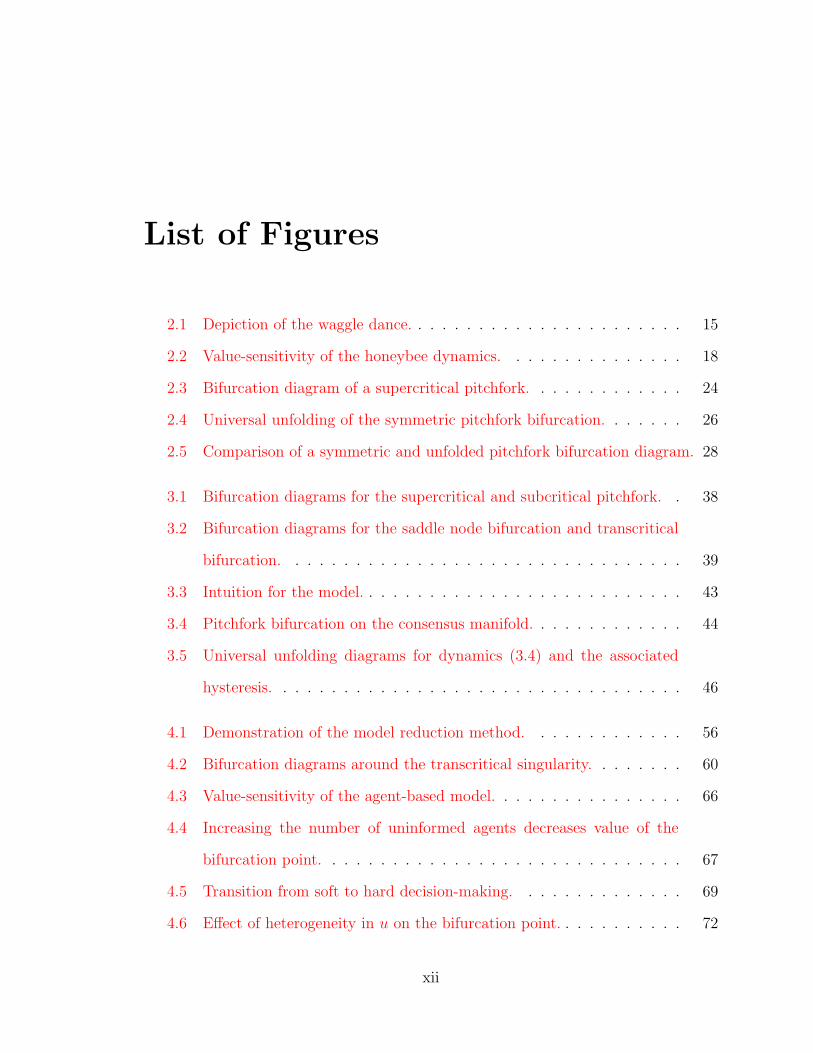
List of Figures
2.1 Depiction of the waggle dance. . . . . . . . . . . . . . . . . . . . . . . 15
2.2 Value-sensitivity of the honeybee dynamics. . . . . . . . . . . . . . . 18
2.3 Bifurcation diagram of a supercritical pitchfork. . . . . . . . . . . . . 24
2.4 Universal unfolding of the symmetric pitchfork bifurcation. . . . . . . 26
2.5 Comparison of a symmetric and unfolded pitchfork bifurcation diagram. 28
3.1 Bifurcation diagrams for the supercritical and subcritical pitchfork. . 38
3.2 Bifurcation diagrams for the saddle node bifurcation and transcritical
bifurcation. . . . . . . . . . . . . . . . . . . . . . . . . . . . . . . . . 39
3.3 Intuition for the model. . . . . . . . . . . . . . . . . . . . . . . . . . . 43
3.4 Pitchfork bifurcation on the consensus manifold. . . . . . . . . . . . . 44
3.5 Universal unfolding diagrams for dynamics (3.4) and the associated
hysteresis. . . . . . . . . . . . . . . . . . . . . . . . . . . . . . . . . . 46
4.1 Demonstration of the model reduction method. . . . . . . . . . . . . 56
4.2 Bifurcation diagrams around the transcritical singularity. . . . . . . . 60
4.3 Value-sensitivity of the agent-based model. . . . . . . . . . . . . . . . 66
4.4 Increasing the number of uninformed agents decreases value of the
bifurcation point. . . . . . . . . . . . . . . . . . . . . . . . . . . . . . 67
4.5 Transition from soft to hard decision-making. . . . . . . . . . . . . . 69
4.6 Effect of heterogeneity in u on the bifurcation point. . . . . . . . . . . 72
xii
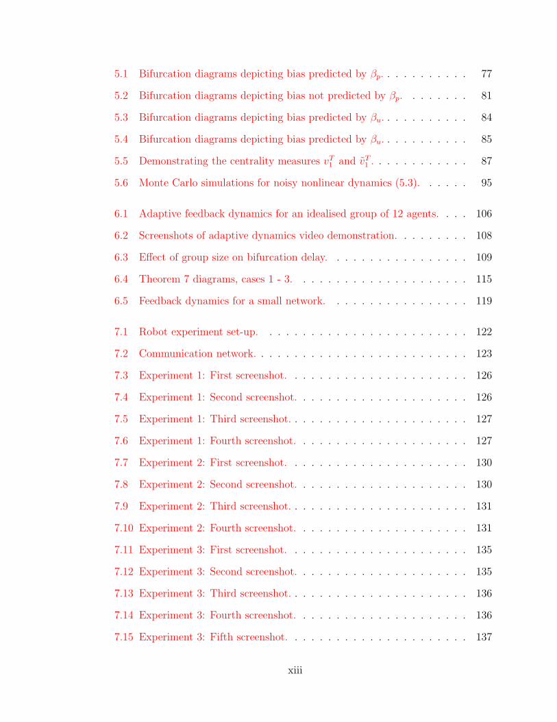
5.1 Bifurcation diagrams depicting bias predicted by βp. . . . . . . . . . . 77
5.2 Bifurcation diagrams depicting bias not predicted by βp. . . . . . . . 81
5.3 Bifurcation diagrams depicting bias predicted by βu. . . . . . . . . . . 84
5.4 Bifurcation diagrams depicting bias predicted by βu. . . . . . . . . . . 85
5.5 Demonstrating the centrality measures vT1 and vT1 . . . . . . . . . . . . 87
5.6 Monte Carlo simulations for noisy nonlinear dynamics (5.3). . . . . . 95
6.1 Adaptive feedback dynamics for an idealised group of 12 agents. . . . 106
6.2 Screenshots of adaptive dynamics video demonstration. . . . . . . . . 108
6.3 Effect of group size on bifurcation delay. . . . . . . . . . . . . . . . . 109
6.4 Theorem 7 diagrams, cases 1 - 3. . . . . . . . . . . . . . . . . . . . . 115
6.5 Feedback dynamics for a small network. . . . . . . . . . . . . . . . . 119
7.1 Robot experiment set-up. . . . . . . . . . . . . . . . . . . . . . . . . 122
7.2 Communication network. . . . . . . . . . . . . . . . . . . . . . . . . . 123
7.3 Experiment 1: First screenshot. . . . . . . . . . . . . . . . . . . . . . 126
7.4 Experiment 1: Second screenshot. . . . . . . . . . . . . . . . . . . . . 126
7.5 Experiment 1: Third screenshot. . . . . . . . . . . . . . . . . . . . . . 127
7.6 Experiment 1: Fourth screenshot. . . . . . . . . . . . . . . . . . . . . 127
7.7 Experiment 2: First screenshot. . . . . . . . . . . . . . . . . . . . . . 130
7.8 Experiment 2: Second screenshot. . . . . . . . . . . . . . . . . . . . . 130
7.9 Experiment 2: Third screenshot. . . . . . . . . . . . . . . . . . . . . . 131
7.10 Experiment 2: Fourth screenshot. . . . . . . . . . . . . . . . . . . . . 131
7.11 Experiment 3: First screenshot. . . . . . . . . . . . . . . . . . . . . . 135
7.12 Experiment 3: Second screenshot. . . . . . . . . . . . . . . . . . . . . 135
7.13 Experiment 3: Third screenshot. . . . . . . . . . . . . . . . . . . . . . 136
7.14 Experiment 3: Fourth screenshot. . . . . . . . . . . . . . . . . . . . . 136
7.15 Experiment 3: Fifth screenshot. . . . . . . . . . . . . . . . . . . . . . 137
xiii

7.16 Experiment 3: Sixth screenshot. . . . . . . . . . . . . . . . . . . . . . 137
7.17 Experiment 4: First screenshot. . . . . . . . . . . . . . . . . . . . . . 139
7.18 Experiment 4: Second screenshot. . . . . . . . . . . . . . . . . . . . . 139
7.19 Experiment 4: Third screenshot. . . . . . . . . . . . . . . . . . . . . . 140
7.20 Experiment 4: Fourth screenshot. . . . . . . . . . . . . . . . . . . . . 140
xiv

Chapter 1
Introduction
1.1 Multi-agent systems
Multi-agent systems are systems comprised of two or more agents that can commu-
nicate and interact with each other. Each agent is capable of autonomous action,
and can also sense and react to its environment [92]. It is common for agents to be
limited in their communication, actuation, computation and sensing abilities, and a
fundamental aim in the study of multi-agent systems is to show that through carefully
designed feedback dynamics and interaction between agents, the system as a whole
can perform complex tasks and produce rich behaviour [58].
Multi-agent systems have many applications in engineering, including mobile sens-
ing networks [24, 56, 57, 73], arrays of micro-devices [4], mobile robotic networks and
power networks [6,14,64]. Multi-agent sensing networks can traverse large or inacces-
sible areas, and extend human capabilities in inhospitable environments [14]. They
can be made up of simple, cheaper agents that are more easily replaceable in the case
of agent failure. Some multi-agent systems may include competitive interactions and
promote individualistic behaviour, but in this thesis we focus on systems that are
cooperative, and are working to achieve a common goal.
1
We also focus on systems that are decentralised, in which each agent uses local
interactions and information to inform its behaviour. Because decentralised systems
do not rely on a central leader, they are robust to agent failures [56]. Often these
decentralised system require simple hardware and computation, as complexity can be
developed through behaviour at the group level, rather than from a single agent. A
multi-agent system may involve heterogeneous agents and asynchronous dynamics [6],
and as such present challenges in coordinating communication and control [4].
We focus on systems that are largely autonomous, but also provide means for
humans to interact with the system in a supervisory role. While full manual control
of a multi-agent system is too high a burden [61], a system should retain the ability
to take advantage of the superior cognitive abilities of a human operator [27]. The
human can provide supervision and task management, and use the data collected by
the agents to develop an overview of the environment and make high-level decisions
[37,56,68].
Some important tasks and objectives for multi-agent systems include decision-
making, formation control, task allocation, distributed estimation and group naviga-
tion [56,64]. In this thesis our focus is on decision-making. We ask the question: how
can a group of agents make a single, collective choice among alternatives?
1.1.1 Collective decision-making
For a multi-agent system, reaching consensus means reaching an agreement regarding
some quantity of interest [66, 67]. For instance, a system of agents performing a
collective task may be required to decide which direction to travel in, what is the
correct value for a measurement being taken, or how to allocate tasks among the
group. Consensus problems have been broadly studied, with a variety of applications
and outcomes. Some examples of consensus problems are the synchronisation of
2
coupled oscillators, coordination of movement for a group of mobile agents, and task
assignment for networked systems [3, 50,77].
In the literature, consensus problems often fall into two main areas of study:
collective sensing and collective decision-making. Collective sensing involves sharing
knowledge to reach an agreement about the true value of a measured environmental
parameter [55, 59, 76, 77]. Agreement must be reached despite limits on the level
and nature of inter-agent interaction, sensor noise and unreliable communication.
Collective decision-making tasks, such as deciding on a direction of travel for the
group, involve reaching an agreement about future group behaviour [60].
In this thesis we focus on collective decision-making, and in particular on a choice
between two alternatives. We present dynamics that allow a group of agents to choose
one of the two alternatives, despite challenges of agent heterogeneity, limited commu-
nication and the possibility of multiple, competing sources of external information.
While some previous studies have combined consensus algorithms with additional dy-
namics, such as dynamics to adjust the direction of travel for agents on the move [60],
here we present general dynamics on the agents’ ‘opinions’ only. These dynamics can
be applied to multiple collective decision-making tasks, and combined with additional
dynamics to achieve complex objectives.
Inspiration from animal behaviour
Collective decision-making dynamics have also been studied in animal groups, in-
cluding situations in which animals rely on successful collective decision-making for
survival. For instance, a swarm of honeybees must quickly and accurately choose a
new nest-site from scouted alternatives that will provide sufficient protection during
the following winter [78–81]. Other examples of collective decision-making in animals
are schooling fish choosing among potential food sources [17, 18, 60], flocks of birds
deciding when to take off together during migration [9,21] and groups of gorillas coor-
3

dinating rest and travel periods [86]. These animal groups are observed to choose with
speed, accuracy, robustness, and adaptability [70], even though they are thought to
be using decentralised strategies and may face limitations on sensing, communication,
and computation [89].
In this dissertation we discuss the honeybee nest-site selection process in detail,
and in particular the contributing mechanisms that allow the bees to make an accurate
and efficient choice from among alternatives. The dynamics of the decision can be
modelled by a pitchfork bifurcation, which captures the remarkable ability of the bees
to remain flexible and to adapt to the environmental conditions while also reliably
reaching an accurate decision. The honeybees perform successfully in the flexibility-
stability trade-off, and provide inspiration for our agent-based model for collective
decision-making.
A first look at the model
In this thesis we present a general agent-based model for collective decision-making
that is organised by a pitchfork bifurcation. The model is nonlinear, and was derived
by Alessio Franci, Vaibhav Srivastava and Naomi Ehrich Leonard [31]. It was designed
to leverage mechanisms from the decision-making dynamics of animal groups for
application in engineered systems, as well as to provide further insights about the
natural systems by studying them from a new perspective. The agent-based model
possesses a pitchfork bifurcation by design, a result that was first proven in [31]. We
refer to the model as “general” because it is not designed for a specific application.
The dynamics model the evolution of each agent’s opinion, which can be thought
of as an internal parameter for each agent. The decision-making dynamics can be
combined with additional dynamics controlling the external behaviour of the agents
to provide successful collective decision-making in the given application.
4
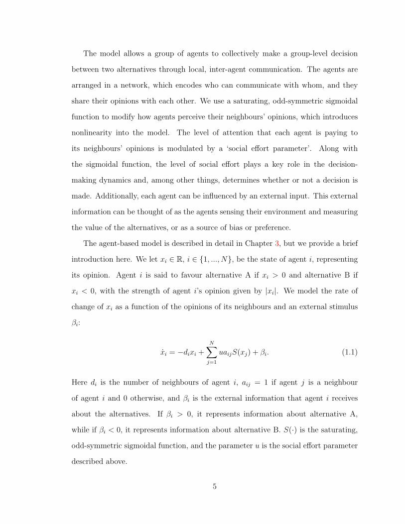
The model allows a group of agents to collectively make a group-level decision
between two alternatives through local, inter-agent communication. The agents are
arranged in a network, which encodes who can communicate with whom, and they
share their opinions with each other. We use a saturating, odd-symmetric sigmoidal
function to modify how agents perceive their neighbours’ opinions, which introduces
nonlinearity into the model. The level of attention that each agent is paying to
its neighbours’ opinions is modulated by a ‘social effort parameter’. Along with
the sigmoidal function, the level of social effort plays a key role in the decision-
making dynamics and, among other things, determines whether or not a decision is
made. Additionally, each agent can be influenced by an external input. This external
information can be thought of as the agents sensing their environment and measuring
the value of the alternatives, or as a source of bias or preference.
The agent-based model is described in detail in Chapter 3, but we provide a brief
introduction here. We let xi ∈ R, i ∈ {1, ..., N}, be the state of agent i, representing
its opinion. Agent i is said to favour alternative A if xi > 0 and alternative B if
xi < 0, with the strength of agent i’s opinion given by |xi|. We model the rate of
change of xi as a function of the opinions of its neighbours and an external stimulus
βi:
xi = −dixi +N∑j=1
uaijS(xj) + βi. (1.1)
Here di is the number of neighbours of agent i, aij = 1 if agent j is a neighbour
of agent i and 0 otherwise, and βi is the external information that agent i receives
about the alternatives. If βi > 0, it represents information about alternative A,
while if βi < 0, it represents information about alternative B. S(·) is the saturating,
odd-symmetric sigmoidal function, and the parameter u is the social effort parameter
described above.
5
The collective decision-making model is an agent-based realisation that was in-
spired by a population-level model for honeybee decision-making dynamics [69, 81],
and the Hopfield network model [45,46]. In [31], Franci et al. showed numerically that
the model retains an important sensitivity to system parameters that was analysed
in [69].
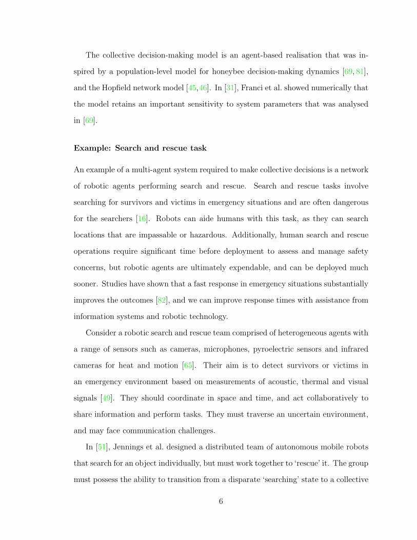
Example: Search and rescue task
An example of a multi-agent system required to make collective decisions is a network
of robotic agents performing search and rescue. Search and rescue tasks involve
searching for survivors and victims in emergency situations and are often dangerous
for the searchers [16]. Robots can aide humans with this task, as they can search
locations that are impassable or hazardous. Additionally, human search and rescue
operations require significant time before deployment to assess and manage safety
concerns, but robotic agents are ultimately expendable, and can be deployed much
sooner. Studies have shown that a fast response in emergency situations substantially
improves the outcomes [82], and we can improve response times with assistance from
information systems and robotic technology.
Consider a robotic search and rescue team comprised of heterogeneous agents with
a range of sensors such as cameras, microphones, pyroelectric sensors and infrared
cameras for heat and motion [65]. Their aim is to detect survivors or victims in
an emergency environment based on measurements of acoustic, thermal and visual
signals [49]. They should coordinate in space and time, and act collaboratively to
share information and perform tasks. They must traverse an uncertain environment,
and may face communication challenges.
In [51], Jennings et al. designed a distributed team of autonomous mobile robots
that search for an object individually, but must work together to ‘rescue’ it. The group
must possess the ability to transition from a disparate ‘searching’ state to a collective
6
‘rescue’ state, a task that requires decision-making and coordination. When surveying
a large area, the group of search and rescue robots must remain close enough to be
able to assemble to perform rescue tasks, and thus they need to be able to collectively
decide where to travel as they search, as well as when to come together for a rescue.
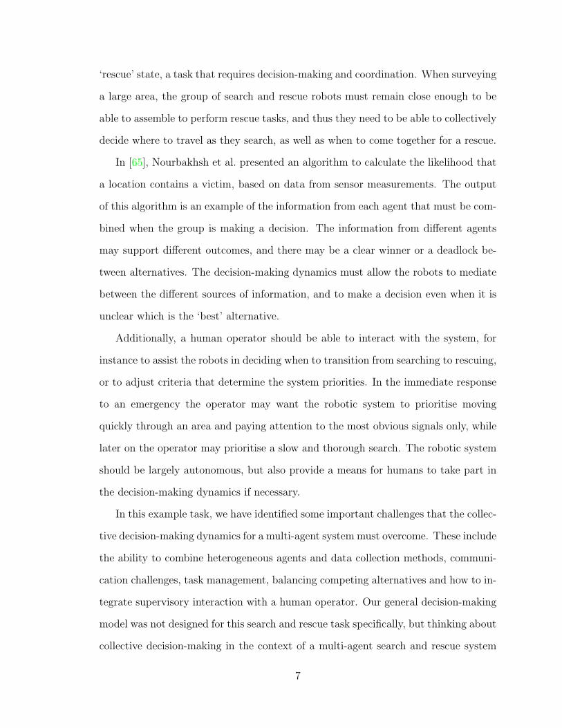
In [65], Nourbakhsh et al. presented an algorithm to calculate the likelihood that
a location contains a victim, based on data from sensor measurements. The output
of this algorithm is an example of the information from each agent that must be com-
bined when the group is making a decision. The information from different agents
may support different outcomes, and there may be a clear winner or a deadlock be-
tween alternatives. The decision-making dynamics must allow the robots to mediate
between the different sources of information, and to make a decision even when it is
unclear which is the ‘best’ alternative.
Additionally, a human operator should be able to interact with the system, for
instance to assist the robots in deciding when to transition from searching to rescuing,
or to adjust criteria that determine the system priorities. In the immediate response
to an emergency the operator may want the robotic system to prioritise moving
quickly through an area and paying attention to the most obvious signals only, while
later on the operator may prioritise a slow and thorough search. The robotic system
should be largely autonomous, but also provide a means for humans to take part in
the decision-making dynamics if necessary.
In this example task, we have identified some important challenges that the collec-
tive decision-making dynamics for a multi-agent system must overcome. These include
the ability to combine heterogeneous agents and data collection methods, communi-
cation challenges, task management, balancing competing alternatives and how to in-
tegrate supervisory interaction with a human operator. Our general decision-making
model was not designed for this search and rescue task specifically, but thinking about
collective decision-making in the context of a multi-agent search and rescue system
7

will allow us to discuss the implications of our general model for design in a specific
setting. We will return to this example throughout this dissertation to illustrate how
the behaviours of our model that we analyse can be applied to improve the design of
collective decision-making dynamics for multi-agent systems.
The flexibility-stability trade-off
An important design consideration that we will return to often in this dissertation is
the flexibility-stability trade-off, which we define here. A stable or robust system is one
in which the desired behaviour will persist in spite of disturbances, while a flexible or
sensitive system is one that can react (for example, respond with different behaviours)
to a variety of parameter regimes. In other words, a robust system should maintain
its behaviour in the presence of inconsequential perturbations, while a flexible system
should be sensitive to meaningful changes, and adapt appropriately. If a system is
required to be both stable and flexible, there is a tension, as in many cases enhancing
one will diminish the other. A successful engineered system must be able to balance
these two requirements in collective decision-making tasks. Fortunately, collective
decision-making and the flexibility-stability trade-off are not unique to engineered
systems, and we can look to other occurrences of these dynamics for inspiration.
1.2 Contributions and thesis outline
In this dissertation, we focus on analysis of the agent-based model, and in particular
how system parameters and the external inputs affect the behaviour. The model
was created for application to the design of engineered systems, and also to allow
further study of the biological sources of inspiration. Here we focus on the design
application, and discuss our results in the context of informing design decisions for
engineered systems.
8

We discuss six important design considerations, which are:
• How can we ensure that the group of agents can make a decision in all circum-
stances?
• How can we improve the ability of the model to remain both sensitive to the
relevant environment parameters but also robust to disturbances (the flexibility-
stability trade-off)?
• How does the communication network affect the behaviour of the system?
• What impact do heterogeneities in the system have on the decision outcome?
• How do internal system and external environmental parameters influence the
behaviour?
• How we can allow humans to interact with the system in meaningful ways?
Our analysis of the model provides answers to these questions, thereby improving
our ability to implement the decision-making dynamics in engineered systems.
In Chapter 2 we discuss the honeybee nest-site selection process, as well as pre-
vious analysis of the honeybee decision-making dynamics. We present results from
the perspectives of both biology and engineering that demonstrate how the bees be-
have and communicate to make efficient and accurate decisions. We also discuss
the decision-making dynamics of schooling fish that must choose between two food
sources, another example of an animal group using local communication to achieve
a collective decision. We then provide an overview of the theory of the pitchfork
bifurcations, a nonlinear phenomenon that is ubiquitous in animal decision-making
and models the remarkable ability of these animal groups to balance flexibility and
stability. We conclude Chapter 2 with a discussion of the six design considerations
9

listed above. We discuss how the biological dynamics provide inspiration for system
design, based on these objectives.
In Chapter 3 we summarise important theory and definitions that are relevant
to this dissertation. In Section 3.2, we present our generalised, agent-based model,
as well as the proof that the model possesses a pitchfork bifurcation. The theorems
and associated proofs in Chapter 3 have been published in [40]. The work from [40]
presented in Chapter 3 was led by Alessio Franci, with contributions from Vaibhav
Srivastava and Naomi Leonard. It has been included in this dissertation because it
provides the foundation for the work that follows. In Section 3.3 we return to our
list of design considerations and discuss how aspects of these have been addressed
implicitly by the design of the agent-based model. From this point forward, this
dissertation represents my contributions to the project.
In Chapter 4 we present a method to reduce the model to a low-dimensional mani-
fold for special cases of graphs. The reduced model provides improved tractability, and
we use the low-dimensional model to analyse additional behaviours to those discussed
in the previous chapter. We discuss how knowledge of each of these behaviours can
be applied to the design of engineered systems that implement the decision-making
dynamics. In Chapter 5 we present results describing the effect of external informa-
tion on the outcome of the decision-making dynamics, and also how the position of
each agent impacts its influence on the group dynamics. We show that these results
persist in the presence of noise.
In Chapter 6 we design an adaptive feedback dynamic on the level of the social
effort parameter u which ensures that the group can always make a decision. The
adaptive dynamic can be ‘switched on’ when it is necessary for the group to reach a
decision, and we discuss how this switch can be triggered both internally by the system
or externally by environmental conditions or a human operator. This discussion leads
us to Chapter 7, where we implement the agent-based decision-making dynamics with
10

a group of three simple robots that must choose which side of a space to drive to. We
performed four experiments with this robotic platform, which demonstrate some of
the behaviours discussed earlier in the thesis, as well as some ways in which a human
operator could interact with the system and control the behaviour at the high-level.
We conclude in Chapter 8 with some summarising remarks, as well as a discussion
of future directions for this work. We briefly discuss some related projects that have
already begun, as well as additional ideas for continuation of this project.
11

Chapter 2
Background: Collective
decision-making organised by a
pitchfork bifurcation
In his book ‘A Honeybee Democracy’ [79] Thomas D. Seeley describes the work of
his academic predecessors Karl von Frisch [33] and Martin Lindauer [62], as well as
his own contributions, to our knowledge of the honeybee Apis mellifera and how
swarms of these bees behave and communicate in order to select a new nest-site. The
passion and delight of these men for their work is clear, and one can easily see why
we now have such a sophisticated and detailed knowledge of many aspects of this
decision-making process. We understand not only the characteristics and qualities,
but also the underlying mechanisms. This understanding places us in a powerful
position to leverage our understanding of honeybee decision-making dynamics for use
in engineered systems. The motive for this chapter is to describe the honeybee nest-
site selection process, the insights we draw from it, and how we can build on this
knowledge in an engineering context.
12

2.1 The honeybee nest-site selection process
In this dissertation, the word ‘honeybee’ is used to describe the species Apis mellifera.
Reproduction of honeybees can be thought of as occurring at two levels; the queen
bee laying eggs to produce new workers, queens or drones, and the colony dividing
to produce new colonies. It is this colony-level reproduction that necessitates the
honeybee nest-site selection process. Roughly half of the existing colony stays behind
in the old nest, while the rest of the bees depart and must find a new home for their
new colony. The bees cluster around the new colony’s queen in a swarm and send
out scouts to search for nest-site candidates, which are typically cavities in trees.
The decision is time sensitive; the bees gorge themselves on honey before leaving and
do not feed again during the decision-making process, so they must choose within a
limited time-frame.
Over spring and summer the worker bees from a hive collect pollen to accumulate
food stores. During the colder months all bees must focus their energy on preserving
warmth in order to stay alive. They cluster together and use a contracting motion
of their flight muscles to produce heat, and rely on stored food for nourishment.
Appropriate nest selection is crucial to successfully enduring the winter, as character-
istics of the nest-site affect the bees’ chance of survival. A summary of their nest-site
preferences and the underlying reasons for them is given in Table 2.1. Typically the
honeybees prioritise sites that provide sufficient storage and shelter. We refer to how
well a site meets these priorities as the value or quality of the site, and use these
terms interchangeably. Poor nest-site selection can lead to the death of the colony
over winter, so the bees must make the high-valued choice accurately. In our agent-
based decision-making model, the value of the alternatives is represented by βi in
(1.1).
During the decision-making process some of the older worker bees, known as
scouts, leave the swarm to search for potential nest-sites and report back to the swarm
13
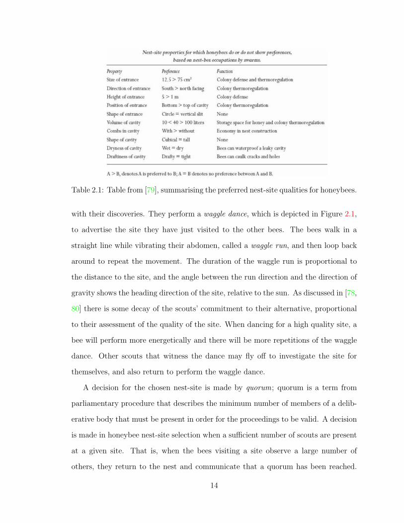
Table 2.1: Table from [79], summarising the preferred nest-site qualities for honeybees.
with their discoveries. They perform a waggle dance, which is depicted in Figure 2.1,
to advertise the site they have just visited to the other bees. The bees walk in a
straight line while vibrating their abdomen, called a waggle run, and then loop back
around to repeat the movement. The duration of the waggle run is proportional to
the distance to the site, and the angle between the run direction and the direction of
gravity shows the heading direction of the site, relative to the sun. As discussed in [78,
80] there is some decay of the scouts’ commitment to their alternative, proportional
to their assessment of the quality of the site. When dancing for a high quality site, a
bee will perform more energetically and there will be more repetitions of the waggle
dance. Other scouts that witness the dance may fly off to investigate the site for
themselves, and also return to perform the waggle dance.
A decision for the chosen nest-site is made by quorum; quorum is a term from
parliamentary procedure that describes the minimum number of members of a delib-
erative body that must be present in order for the proceedings to be valid. A decision
is made in honeybee nest-site selection when a sufficient number of scouts are present
at a given site. That is, when the bees visiting a site observe a large number of
others, they return to the nest and communicate that a quorum has been reached.
14

Figure 2.1: Figure from [79], depicting the waggle dance that is used by scout beesto communicate the distance, direction and quality of a potential nest-site.
Thus, the bees do not require a majority or unanimity to make a selection; once a
quorum of dancers for a given site is reached, that site is chosen. The scouts produce
a particular ‘piping’ sound when the decision is made, and approximately one hour
later, the swarm takes off to inhabit the site that has been chosen. In [80], it is shown
experimentally that the swarms can reliably choose the best nest-site from among
alternatives. This high level of accuracy in choosing the highest valued alternative is
desirable in a decision-making process, and is therefore a characteristic that we want
to leverage for our decision-making model.
In [13], Brown et al. postulated that decisions between two alternatives in a human
brain can be thought of as competition between two populations of neurons, and that
there is cross inhibition between competing populations. We see a similar mechanism
in honeybee decision-making, which gives the bees an efficient way to deal with a
deadlock when choosing between two alternatives that are close in value. Choosing
an alternative when there is a clear winner is a matter of accuracy, but a reliable
decision-making process must also also allow for a decision to be made when the
alternatives are near equal. Decision-making between near-equal alternatives was
the subject of [81], where Seeley et al. showed that the honeybee nest-site selection
process also involves a form of cross inhibition. In addition to the waggle dance, bees
communicate via stop signalling. Neighbouring bees that are not committed to the
same site will head-butt a dancing bee and emit a vibrational signal from their head.
15

Experimental results showed that the accumulation of stop signals will lead to a bee
abandoning their waggle dance. Assuming a well-mixed and large population, a model
for the proportion of bees committed to each alternative, as well as the uncommitted
population, was developed in [81] to study how stop signalling affects the decision-
making process. Seeley et al. showed that with low rates of stop signalling, the
presence of two equal alternatives will lead to a deadlock and no decision being made.
When the stop signalling is occurring at a high rate, the deadlock is broken and one
of the alternatives is chosen at random. The stop signalling allows the bees to make a
decision between equal alternatives. Thus, in addition to a high level of accuracy, the
nest-site selection process also possesses the necessary mechanisms to manage equal
alternatives when an outcome is non-trivial.
Population-level model
The population-level model from [81] was further analysed in [69], to find the critical
value of stop signalling required to break a deadlock between equal alternatives. The
model describes a population of total size N that can be divided into three subpop-
ulations, depending on their commitment or lack thereof to the two alternatives. NA
of the N agents are committed to site A, NB agents are committed to site B and NU
agents have no commitment. The fraction of the population for each of the subpop-
ulations are yA(t) = NA(t)N
, yB(t) = NB(t)N
, and yU(t) = NU (t)N
. The model describes the
evolution of each subpopulations, and because NA+NB +NU = N , yA +yB +yU = 1,
and it suffices to study the evolution of the two committed populations only. The
model encodes the four mechanisms that will result in a change in subpopulation size:
dyA
dt= γAyU − yA(αA − ρAyU + σByB)
dyB
dt= γByU − yB(αB − ρByU + σAyA). (2.1)
16

γi is the rate at which an uncommitted agent discovers and commits to alternative i.
αi is the rate of decay of the commitment of an agent to alternative i and represents
a return to the uncommitted subpopulation. ρi is the rate of recruitment of an
uncommitted agent by an agent committed to alternative i to that alternative, and σi
is the rate of stop signalling between agents with opposing commitment. The assessed
quality of alternative i is νi and, as discussed previously, the experimental results
of [78,80] show that the liveliness and duration of the waggle dance is proportional to
the assessed quality of the site. It is therefore assumed that γi = ρi = νi and αi = 1νi
.
In [69], Pais et al. set σi = σ, and considered a quorum decision to be reached when
yA or yB crosses some threshold ω ∈ (0.5, 1].
Pais et al. showed that when νA = νB = ν, the critical rate of stop signalling
required to break deadlock is given by
σ∗ =4ν3
(ν2 − 1)2. (2.2)
This means that when σ < σ∗, the only option is for the deadlock to remain, but
when σ > σ∗, there are two options, which correspond to a decision for each of the two
alternatives. This transition between the number of possible outcomes (or equilibria)
is called a pitchfork bifurcation, a ubiquitous phenomenon in animal decision-making
between two alternatives [58]. At the critical value of stop signalling σ∗, known as
the bifurcation point, there is a transition from one stable outcome which corresponds
to a deadlock, to two stable outcomes which correspond to a decision for either
alternative, and the deadlock becomes unstable. In Section 2.3, we will discuss the
pitchfork bifurcation in detail, and present the associated theory that is relevant to
this dissertation.
The inverse relationship between the critical value of stop signalling σ∗ and the
assessed value ν given in (2.2) makes the breaking of deadlock sensitive to the value of
17
Stop Signal σ
1 fixed point
3 fixed points
A
B
U
A
B
U
Quality
v
v = 2, σ = 1
v = 3, σ = 5
σ∗ =4v3
(v2 − 1)2
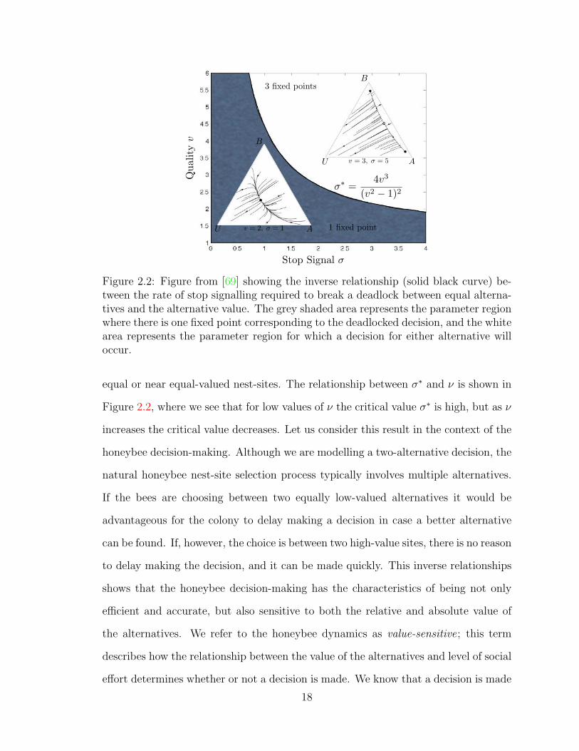
Figure 2.2: Figure from [69] showing the inverse relationship (solid black curve) be-tween the rate of stop signalling required to break a deadlock between equal alterna-tives and the alternative value. The grey shaded area represents the parameter regionwhere there is one fixed point corresponding to the deadlocked decision, and the whitearea represents the parameter region for which a decision for either alternative willoccur.
equal or near equal-valued nest-sites. The relationship between σ∗ and ν is shown in
Figure 2.2, where we see that for low values of ν the critical value σ∗ is high, but as ν
increases the critical value decreases. Let us consider this result in the context of the
honeybee decision-making. Although we are modelling a two-alternative decision, the
natural honeybee nest-site selection process typically involves multiple alternatives.
If the bees are choosing between two equally low-valued alternatives it would be
advantageous for the colony to delay making a decision in case a better alternative
can be found. If, however, the choice is between two high-value sites, there is no reason
to delay making the decision, and it can be made quickly. This inverse relationships
shows that the honeybee decision-making has the characteristics of being not only
efficient and accurate, but also sensitive to both the relative and absolute value of
the alternatives. We refer to the honeybee dynamics as value-sensitive; this term
describes how the relationship between the value of the alternatives and level of social
effort determines whether or not a decision is made. We know that a decision is made
18

for σ > σ∗, and now we also see that the critical stop-signalling level σ∗ depends the
value of the alternatives ν.
Pertinent insights from the honeybee dynamics
We have now seen that the honeybee decision-making dynamics are efficient, accu-
rate and value-sensitive, and possess the necessary mechanisms to make a decision
when the two alternatives are equal. As discussed, the honeybee dynamics can be
modelled by a pitchfork bifurcation, which captures these characteristics, as well as
the remarkable ability of the dynamics to balance flexibility and stability in decision-
making between two alternatives, concepts that we broadly defined in Chapter 1. In
the context of the honeybee dynamics specifically, by flexibility we mean sensitivity
of the decision-making to small differences in the quality of the alternatives, which
can change with changing environmental conditions. By stability, we mean robust-
ness of the decision-making to unwanted disturbances. Since the results from [69,81]
show that these desirable characteristics of flexibility and stability arise from decision-
making that is organised by a pitchfork bifurcation, they motivate the design of an
agent-based model that inherits these advantageous features. In the next section
we consider decision-making dynamics from another animal group, which provided
additional insight and inspiration for our model.
2.2 Decision-making dynamics in schooling fish
In [18], Couzin et al. used numerical simulations to study a large school of fish deciding
between two food sources, when a subgroup of individuals have a prior preference for
one of the two alternatives. They modelled the evolution of the direction of each
fish, which is governed by rules requiring it to swim away from neighbours that are
too close, and swim towards neighbours that are too far away. They also performed
19

experiments in which a number of fish were trained to swim towards one of the
two food sources, introducing a source of external information. They showed that
although the fish in the school are not aware of which individuals are or are not
‘informed’, the simple interactions described above are sufficient for the information
to be communicated to the group.
Couzin et al. performed experiments in which a school of fish must swim towards
one of two food sources. They first considered the case in which the informed in-
dividuals all prefer the same alternative. For large schools, only a small number of
informed individuals are required for the school to make an accurate decision, and to
choose the alternative favoured by the trained individuals. Additionally the propor-
tion of informed individuals required to ensure accuracy decreased with increasing
school size.
When they introduced a second group of informed individuals with a preference
for the other alternative, the decision-making dynamics also exhibited what appeared
to be a pitchfork bifurcation. They considered the symmetric case, where the number
of informed individuals for each alternative was equal. The apparent bifurcation
parameter was the difference in the preferred direction of the two informed groups.
When the degree to which the preferred directions differ was small, the school moved
in the average preferred direction; this is directly analogous to the deadlocked decision
in honeybees discussed in the previous section. As the difference in preferred direction
increased, the school selected one of the two directions with equal likelihood; the
two preferred directions become stables solutions and the average solution becomes
unstable.
Leonard et al. studied this symmetric case in [60], where it was shown that
adding uniformed individuals improves the stability of the collective decision-making.
Leonard et al. defined a continuous-time dynamic model with the same rules governing
the direction of the fish as in [18]. They showed that adding uninformed individuals
20

with no preference increases the parameter region in which a decision is the only sta-
ble solution, and also lowers the critical value of the difference in preferred direction
that is required for a decision to be made. Adding more uninformed individuals was
shown to provide the same effect as increasing the strength of social interaction, and
made the system more robust to parameter variations.
Returning to [18], Couzin et al. showed that if the sizes of the groups of informed
individuals are unequal, the school will reliably choose the alternative favoured by
the majority. This is explained by a phenomenon called an unfolding of the pitchfork
bifurcation, which we will also discuss in Section 2.3 below.
Couzin et al. introduced further asymmetry in [17], where they investigated the
case in which the informed individuals have different preference strengths. They
found that a smaller number of individuals, or a minority, with stronger opinions
could dominate the school outcome over a majority group with weaker opinions when
no uninformed individuals were present. If uninformed individuals were added to
the school, the outcome of the decision could be returned to favouring the majority,
which Couzin et al. described as “inhibiting” the minority group, and “enforcing equal
representation”.
In [18], Couzin et al. postulated that because only a small number of informed
individuals was required to influence the school, having an uninformed population
may be advantageous if the presence of informed individuals is costly. From the
results of [17,60] we also know that the presence of uninformed individuals improves
the ability of the group to make decisions reliably. Leonard et al. showed in [60] that
adding uninformed individuals improves the stability of the decision-making process
to perturbation by enlarging the parameter region for which a decision is ensured.
The results presented in [17,18,60] are either from numerical simulations, or couple
the decision-making dynamics with the movement dynamics. These methods do not
21

allow for easy translation to engineered systems, hence the design of our general,
agent-based model.
Pertinent insights from the schooling fish dynamics
The results from [17,18,60] provide another example of a group of animals that uses
decentralised communication to achieve a group-level consensus, and also of decision-
making dynamics that are organised by a pitchfork bifurcation. The schooling fish
dynamics also provide an example of how asymmetry in the system affects the under-
lying pitchfork bifurcation, leading to an unfolding of the pitchfork. We saw that in-
troducing different-sized informed subgroups, as well as different preference strengths
lead to a bias in the group, which was reflected in the outcome of the decision. Once
we have introduced our general decision-making model, we will analyse and quantify
the effects of asymmetry on the decision-making dynamics. We will return to the
results discussed in this section, particularly the effect of the total group and unin-
formed subgroup size on the dynamics throughout this thesis, as we see similar results
in the analysis of our model.
2.3 The pitchfork bifurcation
We have now seen several examples of decision-making dynamics in biological sys-
tems that display desirable characteristics, and that motivate further study of the
intricacies involved. In this dissertation we present a model that abstracts out the
fundamental properties of these decision-making dynamics and is general enough to
allow us to consider a range of applications. The feature that unites the decision-
making dynamics that we have seen is the pitchfork bifurcation, which appears in
this context as a change from indecision to decision based on a particular system
parameter. The bifurcation occurs at a singularity, and around this singularity there
22
is a heightened sensitivity to changes in parameters, which will allow us to model
the remarkable flexibility of the animal decision-making dynamics in their response
to environmental changes. Away from the singularity the bifurcation dynamics are
robust, which provides stability in the presence of disturbances. By deriving a model
that by design possesses a pitchfork bifurcation, we achieve the desired generalisabil-
ity while maintaining the chosen decision-making dynamics. In this section we review
the relevant bifurcation theory: for a broader understanding see [91] and [88].
Let us begin with the system
y = g(y, u),
where y(t) ∈ R is the resulting trajectory and u ∈ R is a system parameter. From [53],
a point yeq is an equilibrium of the system if
g(yeq, ueq) = 0,
and yeq is a stable equilibrium if for each ε > 0 there exists some δ = δ(ε) > 0 such
that
||y(0)|| < δ =⇒ ||y(t)|| < ε.
An equilibrium point yeq is unstable if it it not stable, and it is asymptotically stable
if it is stable and
||y(0)|| < δ =⇒ limt→∞
y(t) = yeq.
The qualitative behaviour of a system is determined by the pattern of equilibria
(and/or periodic orbits) and their stability, as well as whether this behaviour persists
under small perturbations [53]. A bifurcation is a change in the qualitative behaviour
of the system as the parameter u is varied. This parameter is called the bifurcation
23

parameter, and values of u at which the changes occur are called bifurcation points
(denoted u∗).
We can illustrate these changes in behaviour using a bifurcation diagram, such as
the one given in Figure 2.3, for the system g(y, u) = uy− y3. The diagram shows the
loci of the equilibria over a range of values of the bifurcation parameter u, as well as
the stability of the equilibria. Figure 2.3 shows a supercritical pitchfork bifurcation;
for u < u∗ = 0 there is one stable equilibrium point at y = 0, and for u > u∗ = 0
there are two stable equilibria at yeq = ±√u and one unstable equilibrium point at
yeq = 0. At u = 0, yeq = 0 is a singular point since dgdy
∣∣0,0
= 0. This point is still
stable, but the flow towards it is very slow.
Figure 2.3: Bifurcation diagram of a supercritical pitchfork bifurcation for the systemy = uy− y3. The solid blue lines represent stable equilibria, and the dashed red linesare unstable equilibria. We see that the bifurcation point is at u = u∗ = 0.
When we consider bifurcations in systems with a higher dimensionality, we use
methods that allow us to reduce the number of dimensions while still considering the
salient behaviours [88]. The centre manifold theorem [42, Theorem 3.2.1], tells us
that if f is a vector field on RN , then there are three invariant manifolds W s, W u
and W c that are tangent to the stable, unstable and centre eigenspaces respectively.
The stable (unstable) eigenspace corresponds to the negative (positive) eigenvalues,
while the centre eigenspace corresponds to eigenvalues with zero real parts [91]. If
24
we assume that there are no unstable eigenvalues, the flow will converge along the
stable manifold to the centre manifold and, if this is two-dimensional, we can use
the above bifurcation theory. In this dissertation, the method used to find a two-
dimensional approximation to the system is called the Lyapunov-Schmidt reduction,
and an approachable explanation is given in the first chapter of [35]. This method
involves considering solutions of the N -dimensional system
x = f(x, u)
locally around an equilibrium. We are considering the solutions of f(x, u) = 0. The
Jacobian is the matrix of first-order partial derivates with Jij = dfidxj
. If the Jacobian
of the system at this point is minimally degenerate (having rank N−1) we can divide
the solutions into two sets of equations
Ef(x, u) = 0 (2.3a)
(I − E)f(x, u) = 0, (2.3b)
where E is the projection of RN onto the range of the Jacobian, and I − E is the
complementary projection. (2.3a) can be solved for N − 1 of the variables, which are
then substituted into (2.3b) to give the desired one-dimensional equation, g(y, u) = 0.
g(y, u) = 0 gives the equation for the bifurcation diagram for the reduction of the
N -dimensional system f(x, u).
The normal form of a bifurcation is a simplified form of the system that readily
allows for analysis of the system behaviour. For example, the supercritical pitchfork
bifurcation has the normal form y = uy − y3. In order to prove that our system
exhibits a pitchfork bifurcation, we can prove that our system is equivalent (exhibits
qualitatively similar behaviour) to this normal form using singularity theory [35]. The
singular point of g(y, u) = 0 (a point at which the Jacobian has a zero eigenvalue) is
25

the bifurcation point (y∗, u∗), and as shown in [35, Chapter II] if we can show that
g(y∗, u∗) = gy(y∗, u∗) = gyy(y
∗, u∗) = gu(y∗, u∗) = 0
and
gyyy(y∗, u∗) > 0, guy(y
∗, u∗) < 0
then our system is equivalent to the normal form of a pitchfork bifurcation. Here,
gy = dgdy
and similar for higher orders. This method is the basis for the proof of
Theorem 1. The theorem is presented in Chapter 3 and the proof can be found in
Appendix A.
Figure 2.4: From [35], a universal unfolding of the pitchfork bifurcation. Any per-turbation to the system will lead to one of the four topologically distinct bifurcationdiagrams.
The pitchfork bifurcation shown in Figure 2.3 is a symmetric pitchfork; and is
invariant under the transformation y 7→ −y. Small perturbations to the system
near the singularity will produce changes in the qualitative behaviour, but a powerful
aspect of bifurcation and singularity theory is that we can still characterise all possible
26
behaviours in the presence of these small perturbations. An unfolding is a behaviour
that arises from any small perturbation to the system near the singularity. From [35],
we can define a universal unfolding, G(y, u,α). A universal unfolding for a pitchfork
bifurcation is given by
G(y, u,α) = y3 − uy + α1 + α2y2, (2.4)
and there are just four possible topologically distinct behaviours, as shown in the plot
of the α1, α2 plane in Figure 2.4. Here, α1 and α2 are the unfolding parameters, and
they determine the shape of the bifurcation diagram. Any perturbation of g(y, u) is
equivalent to (2.4) for small α, and can be captured by some combination of α1 and
α2.
In Figure 2.5 we reproduce the symmetric pitchfork of Figure 2.3 with a horizontal
scaling, along with an unfolding from Region (2) of Figure 2.4 overlaid. We can
observe that around the singular point y = 0, u = 1, the unfolded diagram is very
different to the symmetric pitchfork, while away from this point the diagrams are
similar. Close to the singular point, the behaviour of the bifurcation diagram is
very sensitive to parameter changes and this is reflected by the differences between
the diagrams. By inspection of (2.4), we see that close to y = 0, the α1 term,
which is one of the unfolding parameters, will dominate the equation. Far away from
y = 0, the dominant term of (2.4) will be the y3 term, which is not affected by the
unfolding parameters, hence the similarity of the diagram to the symmetric pitchfork.
This observation will prove important in our discussion of the flexibility and stability
properties of dynamics that are organised by a pitchfork bifurcation.
We can see from Figure 2.4 that over a range of the α parameters, we will see
a variety of qualitative system behaviours. We also know that all these behaviours
will occur within a small neighbourhood of α = 0. As described in [35, Chapter I],
27

Figure 2.5: Bifurcation diagram of a symmetric supercritical pitchfork bifurcation(transparent), with the unfolding from region (2) of Figure 2.4 (opaque) overlaid.The solid blue lines represent stable equilibria, and the dashed red lines are unstableequilibria.
an organising centre is an equation that occurs in a model for certain values of pa-
rameters such that most of the system behaviours can be observed within a small
neighbourhood of these values. In other words, most of the bifurcation diagrams that
arise from the dynamics we are describing are captured by a universal unfolding of
this equation. We take inspiration from this concept for our design methodology. The
generalised dynamics that we present model the behaviour of the honeybee dynamics,
and also allow us to consider the role of uninformed individuals that was observed in
the schooling fish. By taking the model through a time-scale change, we also present
a system that can be easily implemented in engineered systems, and allows us to
consider design problems. The model is relevant both to the study of the biological
systems, and also design of dynamics for engineered systems. The model provides
an ‘organising centre’ that allows us to translate insights between these settings. For
another example of work that takes inspiration from the concept of organising centres
for system design, see [30].
28

2.3.1 The flexibility-stability trade-off
We defined the flexibility-stability trade-off in Chapter 1 and discussed in Section 2.1
how the honeybee nest-site selection process performs remarkably in the flexibility-
stability trade-off. The sensing and communication tasks that make up the decision-
making process are carried out by individual bees, and will likely involve some error,
but the process remains stable. Additionally, the bees reliably make a decision when
there is a clearly superior alternative and also when there are alternatives that are
nearly equal. The dynamics are also flexible, due to the apparent value-sensitivity of
the bees to both the relative and absolute values of the alternatives.
The trade-off between flexibility and stability, as well as successful realisation of
both properties is widely studied in neurophysiological systems, where it has been
shown that the nervous system can produce stable behaviour despite perturbations
but also respond flexibly to component variation [63]. Nonlinear models that allow
for both flexibility and stability can be found in [19, 20, 28], but little work has been
done to understand this trade-off in other settings.
Now that we have an overview of the pitchfork bifurcation theory, we can begin
to understand how it models the ability to cope with both unwanted disturbances
and legitimate perturbations, and allows us to translate the favourable properties
of honeybee nest-site selection to our system. As we saw in the previous section, a
universal unfolding of a pitchfork captures the four possible ways in which a system
can change in response to disturbance, so there are a finite number of predictable
behaviours. Recall from Section 2.3, we discussed how the behaviour of the unfolding
of the pitchfork bifurcation is very different to the symmetric bifurcation close to the
bifurcation point, and very similar to the symmetric bifurcation far away from the
bifurcation point. This effect, which is illustrated in Figure 2.5, shows how systems
that exhibit a pitchfork bifurcation are highly sensitive to parameter changes around
the bifurcation point, and highly robust to changes far away from the bifurcation
29

point. This is an important concept that we will return to throughout this dissertation
and we will see numerous examples that illustrate this behaviour.
The discussion of the flexibility and stability of our proposed model is continued
in Chapter 3, where we describe further how the pitchfork bifurcation allows for an in-
herently successful performance in the flexibility-stability trade-off. Throughout this
thesis, as we continue to investigate the behaviour of our agent-based model, we will
return to these notions of flexibility and stability. We will see how the new behaviours
of the model that we have analysed further contribute to successful performance in
this trade-off.
2.4 Design of engineered systems
The honeybee decision-making dynamics described in this chapter provide inspira-
tion for our agent-based model, which can be applied to engineering applications that
require network-level decision-making among alternatives. As outlined in previous
sections, we have a deep understanding of the desirable qualities of the honeybee
decision-making dynamics, as well as the underlying mechanisms that can produce
these outcomes, and we may now apply them to our dynamics. The collective decision-
making model presented in this thesis was designed to accomplish two main aims:
both to leverage the successful mechanisms of the nest-site selection process for ap-
plication in engineered systems and also to ask further questions about the biological
decision-making dynamics. In this dissertation, we focus on the former aim, and in
particular on how the insights gained as we study the model can be applied to the
design of engineered systems. We are not confined by the intrinsic parameter regimes
of the natural systems, and we can explore new possibilities in the engineering setting.
Let us now return to the example of a robotic search and rescue task, and discuss
the design considerations and objectives that would arise when applying decision-
30

making dynamics to this multi-agent system, as well as the sources of inspiration
from the biological dynamics and the tools from engineering that we will use to
address these objectives.
Transition from deadlock to decision: When we introduced the example of search
and rescue task, we discussed a study by Jennings et al. [51] in which the robots were
required to autonomously transition between performing search tasks separately, and
rescue tasks collectively. In the honeybee decision-making dynamics, we saw that it
is crucial that the honeybees reach a group decision, and that they use stop signalling
to break a deadlock between near equal alternatives. The stop signalling facilitates a
transition from deadlock to decision, and we use a similar parameter in our model. It
was postulated in [69] that the rate of stop signalling might gradually increase over
time, to ensure that the bees reach a decision. We take inspiration from this to design
an adaptive feedback dynamic which ensures a decision is made.
Flexibility-stability trade-off : Robotic agents performing a search and rescue task
will likely operate in an uncertain environment, and therefore successful performance
in the flexibility-stability trade-off is a key requirement. When searching for signs of
human life it is crucial that the robotic agents do not overlook true signals, but the
task is also time-sensitive so the system cannot afford to be constantly disrupted by
false signals. As we have seen, decision-making dynamics organised by a pitchfork
bifurcation possess an innate ability to balance flexibility and stability, and this is a
quality that our model should also possess. We use the tools of nonlinear systems
analysis [41] and bifurcation analysis via singularity theory [36] to demonstrate that
our model possesses a pitchfork bifurcation, and therefore the associated flexibility
and stability properties.
Influence of the network structure: If the search and rescue task is being carried
out in response to a natural disaster, there will likely be limitations on, or disruption
of, communication. To ensure successful performance despite these limitations, it is
31

crucial to know how the communication network will affect the system performance
and behaviour. The previous population level models of the honeybee dynamics
studied in [69, 81] do not accommodate examination of the role of communication
networks, and do not allow easy translation of the mechanisms from the honeybee
dynamics to a multi-agent system. The agent-based model presented in this thesis
considers a group of agents arranged in a communication network, and allows us to
encode a network structure into the model. We can then analyse the effect of the
network structure on system performance using graph theory [64], which will inform
design decisions when implementing the decision-making model.
The role of heterogeneity in the system: A robotic search and rescue system may
consist of heterogeneous agents with differing sensors and communication abilities,
which must all be incorporated into the group dynamics. Also, in some cases, hetero-
geneity in a system can be advantageous; if sensing equipment is costly then we may
wish to design a system in which agents are fitted with varying qualities of sensors.
Additionally, in [17,60], the authors showed evidence that adding uninformed individ-
uals to the group returned the decision-making dominance to a majority, which was
previously dominated by a minority with stronger opinions. We will investigate the
role of heterogeneity in our model. Adding heterogeneity to the system adds complex-
ity, which can limit our abilities to analyse the dynamics. We can use tools such as
the centre manifold theorem [41], the Lyapunov-Schmidt reduction [36] and LaSalle’s
invariance principle [53] to describe the behaviour of complex, high-dimensional sys-
tem in lower dimensions. We can perform the necessary analysis while maintaining a
level of complexity in the original system that allows us to consider heterogeneity.
Effect of system parameters : In addition to designing systems that balance flex-
ibility and stability, we can improve the performance of our engineered systems by
developing a strong understanding of how system parameters affect the behaviour. As
we discussed in Section 2.1, during the honeybee decision-making process the rate of
32
stop signalling between bees determines whether or not a decision is made when the
swarm is choosing between two alternatives of equal value. As shown in [69] the rate
of stop signalling required to break a deadlock is inversely proportional to the value
of the two alternatives. This value-sensitivity would allow the bees to delay making
a decision when they are choosing between two equally low-valued alternatives, and
make a decision quickly when choosing between high-valued alternatives. In a search
and rescue task, it would be advantageous to design decision-making dynamics that
lead to a quick decision when the agents have a high level of confidence in their sen-
sor measurements, but can delay making a decision when their confidence level is
low. We can use techniques from applied mathematics such as asymptotic expansion
and spectral analysis to improve our understanding of how system parameters affect
the behaviour, and how we can design system dynamics that take advantage of the
properties that we discover.
Incorporating human interaction: As discussed in Chapter 1, humans taking
part in the search and rescue task should be able to interact with the robotic
system in a manner that takes advantage of our superior cognitive abilities, without
overburdening the human operator with unnecessary decisions and responsibilities.
This design consideration has no parallel in the honeybee decision-making dynamics,
and requires us to think beyond the biology. We implement our decision-making
dynamics in a small robotic network, and the results of these experiments allow us to
think about how human operators could control system behaviour through simple,
high-level interactions.
In this chapter we have learnt of the sources of inspiration for the agent-based
model for collective decision-making presented in this thesis; the dynamics of house-
hunting honeybees and schooling fish. We have discussed the pitchfork bifurcation,
which is ubiquitous in two-choice animal decision-making, and models the abilities
33

of these animals groups to perform successfully in the flexibility-stability trade-off.
In the next chapter we describe our generalised decision-making model and show
that, by design, it possesses the pitchfork bifurcation. We see that some of the
design considerations mentioned here are addressed by the inherent properties of the
dynamics, while others require further study.
34
Chapter 3
The agent-based model for
collective decision-making
In this chapter we provide the theory, terms and notation that are relevant for this
thesis. We then present the generalised, agent-based model for collective decision-
making, and prove that it exhibits a pitchfork bifurcation. The model was first
presented in [31] by Alessio Franci, Vaibhav Srivastava and Naomi Ehrich Leonard,
who together formed the idea and approach for the model and derived the model along
with an early version of the proof that it contains a pitchfork bifurcation. In my work
I have analysed, extended and applied the model in various contexts, and aspects of
my work have been published in [39] and [40]. I was the lead author for [39] and the
lead contributor to the analysis, results, discussion and writing. Alessio Franci and
Vaibhav Srivastava provided the proof that a specialised case of the model contains
the pitchfork bifurcation which is presented here as Corollary 2, and along with Naomi
Ehrich Leonard contributed to and provided guidance for all aspects of the work. I
was the joint lead author for [40] along with Alessio Franci. Alessio Franci was the
lead contributor to the sections discussed in this chapter, in particular Theorems 1
35
and 3 and the associated proofs given in Appendix 1. Vaibhav Srivastava and Naomi
Ehrich Leonard provided guidance and contributed to all aspects of the work.
In the following chapter, in Section 3.2, the mathematical description of the vari-
ables, the model, its extensions and Theorem 1, Corollary 2 and Theorem 3 are taken
verbatim from [40], and were mostly written by Alessio Franci. Figure 3.5 was cre-
ated by myself for [40] and Figure 3.3 is original. All other sections as well as some
explanations and discussion in Section 3.2 are original.
3.1 Relevant theory, terms and notation
We wish to consider a group of N individuals performing a decision-making task
together, and we refer to each member of the group as an agent. Some examples of
possible agents are honeybees, fish, or robots in a sensing network. Throughout the
decision-making process, we keep track of the opinion of each agent, i ∈ {1, . . . , N},
which is represented as a state variable xi ∈ R. Information about who communicates
with whom is encoded into the model through network representation.
Network representation and theory
For a network of N agents, agent i is able to measure the opinion of agent j if there
is a directed edge in the network from agent i to agent j, in which case we say that
j is a neighbour of i. This information is encoded in a network adjacency matrix A.
We define the entries of A using the following rules:
aij =
0 if j is not a neighbour of i, and for j = i
1 if j is a neighbour of i.
We use network diagrams to visually represent a network, such as the network de-
picted on the far right of Figure 3.5. We use the convention that an arrow directed
36
from agent i to agent j means that agent i is sensing agent j. Small black arrows
represent individual communication, and block white arrows represent all-to-all com-
munication between subgroups of agents.
We define D, a diagonal matrix with entries di, known as the degree of each
agent. We use di =∑N
j=1 aij, known as the in-degree, and∑N
i=1 aij is the out-degree.
A network is undirected if for every i, j ∈ {1, ..., N}, aij = aji, and directed if this is
not the case. If the in-degree and out-degree are equal, a network is balanced, which
is always the case for an undirected network. A directed network is connected if there
exists a directed path (sequence of directed edges) between each pair of nodes, and
is strongly connected if there are directed paths in both direction between each pair.
An all-to-all graph, also known as a complete graph, contains undirected edges that
connect all nodes.
L = D − A is the Laplacian matrix of the graph; it is a powerful tool for the
analysis of a network’s performance in consensus tasks. If we consider the linear
consensus dynamic
x = −Lx, (3.1)
because each di =∑N
j=1 aij, every row of the network Laplacian will sum to zero,
so therefore the matrix L will have a zero eigenvalue corresponding to the (right)
eigenvector ζ1N , with ζ ∈ R. If the network represented by L is strongly connected,
there will be only one zero eigenvalue; this means that ζ1N is in the nullspace of L, so
the dynamics (3.1) will converge to a consensus [23, 66]. Additionally, the remaining
N − 1 eigenvalues of a strongly connected Laplacian L are positive.
We will also refer to the left eigenvector of L corresponding to the null eigenvalue
often throughout this thesis, which we denote vT1 . We use the result that vT1 1N 6= 0,
which we will now prove here. Again assuming a strongly connected graph, we may
37

write the Laplacian matrix L in Jordan normal form [87] J = PAP−1, such that
J =
λ1 0
0 M
,where M is a matrix of the Jordan blocks for the remaining N − 1 eigenvalues. We
know that vT1 = eT1 P−1 and 1N = Pe1, where ei is the i-th vector of the standard
basis for RN . Therefore
vT1 1N = eT1 P−1Pe1
= 1 6= 0. �
Henceforth, the vector vT1 is normalised such that vT1 1N =√N .
Types of bifurcation diagram
Figure 3.1: Left: Bifurcation diagram of a supercritical pitchfork bifurcation. Right:Bifurcation diagram of a subcritical pitchfork bifurcation. For both diagrams thesolid blue lines represent stable equilibria, the dashed red lines are unstable equilibriaand the bifurcation point is at u = u∗ = 0.
In addition to the supercritical pitchfork bifurcation described in Chapter 2 we
will encounter other types of bifurcation in this thesis, which are summarised here.
Another form of pitchfork bifurcation is the subcritical pitchfork bifurcation, which
38

has the normal form y = uy + y3. Unlike the supercritical pitchfork, where there is a
change from one stable equilibrium, to two stable and one unstable equilibria at the
bifurcation point, the subcritical pitchfork involves a change from one stable and two
unstable equilibria to one unstable equilibrium. The two pitchfork bifurcations are
shown side-by-side in Figure 3.1.
Figure 3.2: Left: Bifurcation diagram of a saddle-node bifurcation. Right: Bifurcationdiagram of a transcritical bifurcation. For both diagrams the solid blue lines representstable equilibria, the dashed red lines are unstable equilibria and the bifurcation pointis at u = u∗ = 0.
A saddle-node bifurcation has the normal form y = u+y2, and is characterised by
the appearance of one stable and one unstable node at the bifurcation point. Prior to
the bifurcation point there are no equilibria. A saddle-node bifurcation is depicted in
Figure 3.2 (left). A transcritical bifurcation has the normal form y = uy− y2, and as
shown in Figure 3.2 (right) the two equilibria persist before and after the bifurcation
point, but exchange stabilities. As shown in Chapter 4, under certain parametric
conditions our model will produce bifurcation behaviour that is a combination of
these types of bifurcation.
39
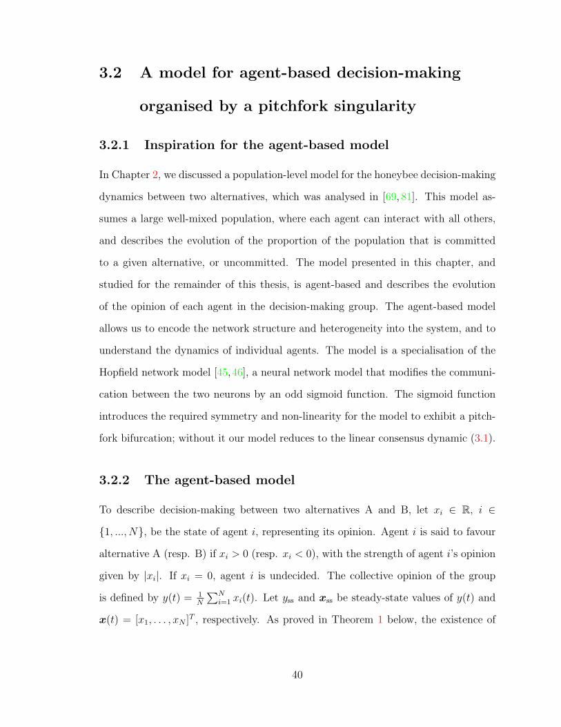
3.2 A model for agent-based decision-making
organised by a pitchfork singularity
3.2.1 Inspiration for the agent-based model
In Chapter 2, we discussed a population-level model for the honeybee decision-making
dynamics between two alternatives, which was analysed in [69, 81]. This model as-
sumes a large well-mixed population, where each agent can interact with all others,
and describes the evolution of the proportion of the population that is committed
to a given alternative, or uncommitted. The model presented in this chapter, and
studied for the remainder of this thesis, is agent-based and describes the evolution
of the opinion of each agent in the decision-making group. The agent-based model
allows us to encode the network structure and heterogeneity into the system, and to
understand the dynamics of individual agents. The model is a specialisation of the
Hopfield network model [45,46], a neural network model that modifies the communi-
cation between the two neurons by an odd sigmoid function. The sigmoid function
introduces the required symmetry and non-linearity for the model to exhibit a pitch-
fork bifurcation; without it our model reduces to the linear consensus dynamic (3.1).
3.2.2 The agent-based model
To describe decision-making between two alternatives A and B, let xi ∈ R, i ∈
{1, ..., N}, be the state of agent i, representing its opinion. Agent i is said to favour
alternative A (resp. B) if xi > 0 (resp. xi < 0), with the strength of agent i’s opinion
given by |xi|. If xi = 0, agent i is undecided. The collective opinion of the group
is defined by y(t) = 1N
∑Ni=1 xi(t). Let yss and xss be steady-state values of y(t) and
x(t) = [x1, . . . , xN ]T , respectively. As proved in Theorem 1 below, the existence of
40

yss and xss is ensured by the boundedness of trajectories and the monotonicity of the
proposed model.
Let the group’s disagreement δ be defined by δ = |yss|− 1N‖xss‖1, where ‖·‖1 is the
vector 1-norm. If each entry of xss has the same sign, then there is no disagreement,
i.e., δ = 0. We say that the group’s decision-making is in deadlock if either xss = 0
(no decision) or δ 6= 0 (disagreement). A collective decision is made in favour of
alternative A (resp. B) if δ = 0 and yss > η (resp. yss < −η), for some appropriately
chosen threshold η ∈ R>0.
We model the rate of change in state of each agent over time as a function of the
agent’s current state, the state of its neighbours, and a possible external stimulus νi:
dxidt
= −uIdixi +N∑j=1
uSaijS(xj) + νi. (3.2)
Here, νi ∈ R encodes external information about an alternative received by agent i,
or it represents the agent’s preference between alternatives (we will use “information”
and “preference” interchangeably). We let νi ∈ {νA, 0,−νB}, νA, νB ∈ R+. If νi = νA
(resp. νi = −νB) agent i is informed about, or prefers, alternative A (resp. B). If
νi = 0 agent i receives no information or has no preference. uI > 0 and uS > 0 are
control parameters and S : R→ R is a smooth, odd sigmoidal function that satisfies
the following conditions: S ′(z) > 0, ∀z ∈ R (monotone); S(z) belongs to sector
(0, 1]; and sgn(S ′′(z)) = −sgn(z), where (·)′ denotes the derivative with respect to
the argument of the function, and sgn(·) is the signum function.
The control uI can be interpreted as the inertia that prevents agents from rapidly
developing a strong opinion. The term uSaijS(xj) can be interpreted as the opinion
of agent j as perceived by agent i. Since S(x) is a saturating function, opinions of
small magnitude are perceived as they are, while opinions of large magnitude are
41

perceived as saturating at some cap. The control uS represents the strength of the
social effort : a larger uS means more attention is paid to other agents’ opinions.
Let ν = (ν1, . . . , νN)T , and S(x) = (S(x1), . . . , S(xN))T . Then (3.2) can be
written in vector form as
dx
dt= −uIDx+ uSAS(x) + ν. (3.3)
To simplify notation, we study (3.3) using a time-scale change s = uIt. We denote
x(s) by x and dx/ds by x. Let u = uS/uI , βi = νi/uI , βA = νA/uI , βB = νB/uI and
β = (β1, . . . , βN)T . Then each βi ∈ {βA, 0,−βB} and (3.3) is equivalent to
x = −Dx+ uAS(x) + β. (3.4)
To provide intuition for the model, let us consider the simplest possible network of
two agents, depicted in the Figure 3.3. We model the interaction between these agents
in the block diagram shown in Figure 3.3 (top). Each agent receives information
about the environment via a scalar parameter βi and a negative feedback on the
agent’s own opinion which drives the opinions back towards zero and prevents a large
opinion developing quickly. In addition, there is a positive feedback of information
about the opinion of its neighbour via the function block uS(xi). The sigmoidal
term S(xi) has a saturating effect on how the agent’s opinion is perceived, and the
parameter u modulates the size of this effect. The effect of the function block uS(xi)
is illustrated in Figure 3.3 (bottom). We plot nullclines of this system for β = 0
with S(·) = tanh(·), and we see that for small u and u < 1 we have one intersection
at zero which represents a deadlock (no decision). The negative feedback, shown in
blue is dominant and drives the opinions back towards zero. As u is increased the
positive feedback in red destabilises the deadlock solution and we see the appearance
of two more equilibria representing a decision for the one of the two alternatives. The
42
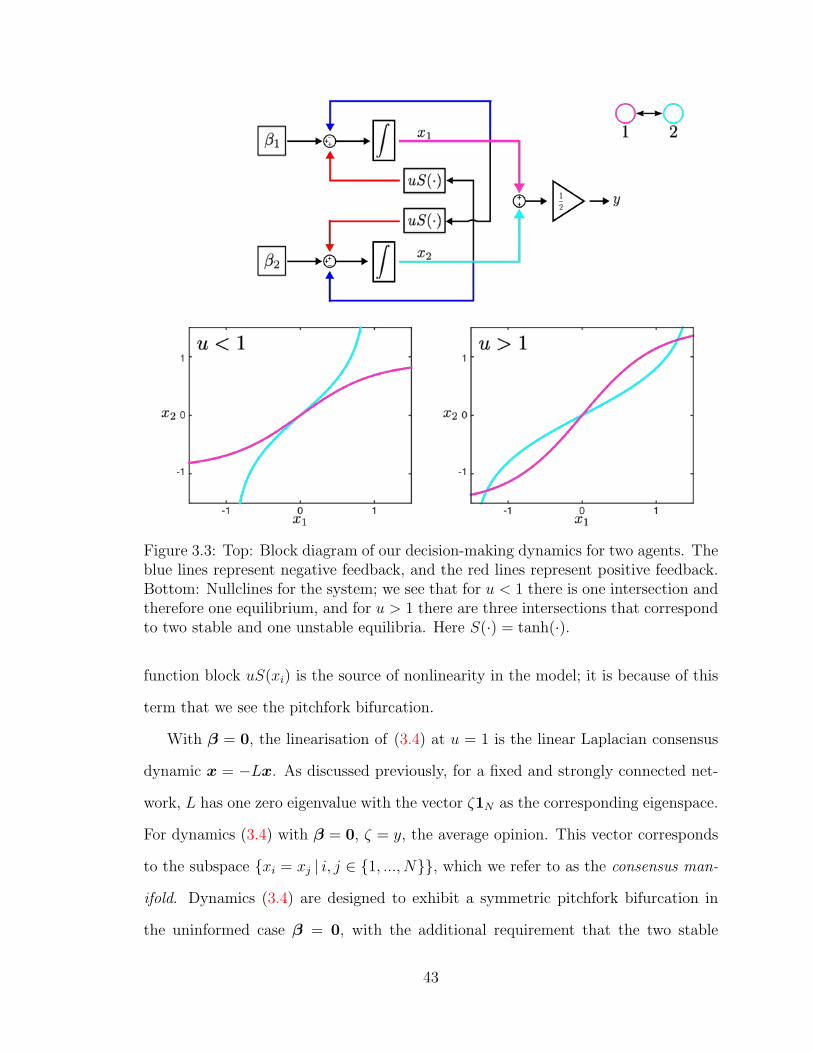
Figure 3.3: Top: Block diagram of our decision-making dynamics for two agents. Theblue lines represent negative feedback, and the red lines represent positive feedback.Bottom: Nullclines for the system; we see that for u < 1 there is one intersection andtherefore one equilibrium, and for u > 1 there are three intersections that correspondto two stable and one unstable equilibria. Here S(·) = tanh(·).
function block uS(xi) is the source of nonlinearity in the model; it is because of this
term that we see the pitchfork bifurcation.
With β = 0, the linearisation of (3.4) at u = 1 is the linear Laplacian consensus
dynamic x = −Lx. As discussed previously, for a fixed and strongly connected net-
work, L has one zero eigenvalue with the vector ζ1N as the corresponding eigenspace.
For dynamics (3.4) with β = 0, ζ = y, the average opinion. This vector corresponds
to the subspace {xi = xj | i, j ∈ {1, ..., N}}, which we refer to as the consensus man-
ifold. Dynamics (3.4) are designed to exhibit a symmetric pitchfork bifurcation in
the uninformed case β = 0, with the additional requirement that the two stable
43
x i
− x j u
x i = x j
Figure 3.4: For u = 1 and β = 0, dynamics (3.4) exhibit a pitchfork bifurcation atx = 0. The steady-state branches emerging at the singularity lie on the consensusmanifold {xi = xj | i, j ∈ {1, ..., N}} shown in grey. Branches of stable and unstablesolutions are shown as solid and dashed lines, respectively.
steady-state branches emerging at the pitchfork do so along the consensus manifold.
In other words, we have designed dynamics (3.4), equivalently dynamics (3.3), with
β = 0 as a model of unanimous collective decision-making between two alternatives.
It follows from the center manifold theorem [41, Theorem 3.2.1] that (3.4) possesses
a one-dimensional invariant manifold that is tangent to the consensus manifold at
the origin. On this manifold, the reduced one-dimensional dynamics undergo a bi-
furcation, which, by odd (that is, S2) symmetry of (3.4) with β = 0, will generically
be a pitchfork [35, Theorem VI.5.1, case (1)]. A geometric illustration for N = 2
with β = 0 is given in Figure 3.4. The grey plane represents the consensus manifold
xi = xj on which the steady-state bifurcation dynamics evolve.
For β 6= 0 there is an additional term in the linearisation and the opinion values
x 6= ζ1N . For sufficiently small β the opinions remains close to ζ1N , and we say that
the consensus manifold has been perturbed.
A note on Z2 and S2 symmetry
Several results in this thesis rely on the Z2 symmetry of our dynamics. On R, the
group Z2 can be represented by the set {1,−1}, where the element 1 maps y ∈ R
to y and the element −1 maps y ∈ R to −y. When we say our dynamics are Z2
symmetric, we imply that they are invariant under the transformations that result
44

from the action of the Z2 group. Our model is Z2 symmetric because it is odd
symmetric. In our modelling approach, we represent the alternative A by positive
values and the alternative B by negative values, so multiplying by the element −1
corresponds to swapping the alternatives.
The finite symmetric group S2 is the set of permutations that can be performed
on a set of two symbols, and has two elements: the identity and the element that
swaps the two symbols. S2 is isomorphic to Z2 (from an abstract group theoretical
perspective, they are the same order-two group generated by {e, a}, where e is the
identity and a2 = e). From an option permutation perspective, our model is thus
both S2 and Z2 symmetric, and we may use these terms interchangeably.
3.2.3 A pitchfork bifurcation by design in generic networks
A preliminary version of the following theorem can be found in the preprint [31].
Theorem 1. [40] The following hold for the dynamics (3.4) where the graph is fixed
and strongly connected:
i. For β = 0, x = 0 is globally asymptotically stable if 0 < u ≤ 1, and locally
exponentially stable if 0 < u < 1.
ii. Let g(y, u,0) be the Lyapunov-Schmidt reduction of (3.4) at (x, u) = (0, 1) for
β = 0. The equilibria satisfying g(y, u,0) = undergo a symmetric pitchfork
singularity at (x∗, u∗) = (0, 1). For u > 1 and |u − 1| sufficiently small the
Jacobian of (3.4) at x = 0 possesses a single positive eigenvalue and all other
eigenvalues are negative. The (N−1)-dimensional stable manifold separates the
basins of attraction of the other two steady states bifurcating from the pitchfork,
which attract almost all trajectories. Further, the steady-state branches bifur-
cating from the pitchfork for u > 1 are exactly the origin and ±ys1N , where
{0,±ys} are the three solutions of the equation y − uS(y) = 0, u > 1.
45

iii. For β 6= 0, the solutions to g(y, u,β) = 0 undergo an N-parameter unfolding of
the symmetric pitchfork. Moreover ∂g∂βi
(0, 1,0) = vT1 ei, where vT1 is a null left
eigenvector of L and ei is the i-th vector of the standard basis of RN .
The proof for Theorem 1 can be found in Appendix 1. Theorem 1 proves that
dynamics (3.4) possess a pitchfork bifurcation, and therefore the associated qualities
of decision-making dynamics that are organised by this phenomenon. When β =
0, there is a symmetric pitchfork bifurcation, and for u > u∗ there are two stable
solutions that represent a decision for either of the two alternatives. For β 6= 0 we
see an unfolding of the symmetric pitchfork.
Figure 3.5: Figure taken from [40]. Left: the four persistent bifurcation diagramsof a universal unfolding of the pitchfork in model (3.4), for the network shown onthe right. Blue lines are stable solutions and red lines unstable solutions. Right:Hysteresis behaviour in the unfolding of the pitchfork. The graph topology and thedistribution of βi values is represented by the node colour, with βA = 5 and βBvarying. White arrows represent all-to-all directed connections from one populationto another and u = 1.5.
Figure 3.5 (left) shows the four persistent bifurcation diagrams in a universal
unfolding of the pitchfork in dynamics (3.4) for the network shown on the far right.
The agents in green have information value βA, for alternative A, and the agents in
pink have information value βB, for alternative B. As stated in Theorem 1, part (iii),
the scalar representation of dynamics (3.4), g(y, u,β), is an N -parameter unfolding
46

of the symmetric pitchfork. By changing the values of βA and βB, we can reproduce
the four diagrams from Figure 2.4. β enters dynamics (3.4) linearly, so most often
we will see diagrams I and II. However, asymmetry due to the network structure also
causes an unfolding, and we can exploit this to realise the remaining two diagrams. In
order to move throughout all regions of Figure 2.4, we must manipulate both the α1
and α2 parameters. Due to the formulation of (3.4) we can only change α1 explicitly
via changing β. We can implicitly manipulate α2 by changing the network structure
and information distribution, but we don’t have an analytical relation to guide us.
Figure 3.5 (right) shows the hysteresis that occurs when we fix βA and u and vary
the value of βB. Let us begin at in the bottom left corner of Figure 3.5 (right), close
to (0, -1). Here, βA = βB, but due to asymmetry in the network structure, y = −1
and alternative B is preferred. The bifurcation diagram would look like diagram I in
Figure 3.5 (left). As we decrease βB and move to the right in Figure 3.5 (right), close
to (1, -1), the bifurcation diagram would change to look like diagram II of Figure 3.5
(left). Although the positive branch of II has become stable for low u values, due
to the bistability of solutions we remain on the negative branch. As we continue to
increase βA − βB, and move to the far right of Figure 3.5 (right), the saddle node
that creates the negative branch in II also moves to the right, until eventually there is
only one stable equilibria for the current value of u. At this point the solution jumps
to the positive branch of II and the upper branch in Figure 3.5 (right). We see this
effect in reverse as βB increases. What this means for dynamics (3.4) is that once a
decision has been made for an alternative even if there are small perturbations to the
perceived alternative values, the decision will persist. However, if there are significant
changes to the alternative values, the dynamics will respond by making a different
decision. This hysteresis behaviour contributes to the robustness of the dynamics, as
we will discuss below. As shown in [69], the same hysteresis behaviour was observed
for the population-level model of the honeybee decision-making dynamics.
47

All-to-all networks
In an all-to-all network and β = 0, the dynamics (3.4) specialize to
xi = −(N − 1)xi +N∑
j=1,j 6=i
uS(xj), (3.5)
and Theorem 1 holds globally in u and x.
Corollary 2. [40] The following statements hold for the stability of invariant sets of
dynamics (3.5):
i. The consensus manifold {xi = xj | i, j ∈ {1, ..., N}} is globally exponentially
stable for each u ∈ R, u ≥ 0;
ii. x = 0 is globally exponentially stable for u ∈ [0, 1) and globally asymptotically
stable for u = u∗ = 1;
iii. x = 0 is exponentially unstable and there exist two locally exponentially stable
equilibrium points ±ys1N for u > 1, where ys > 0 is the positive non-zero
solution of −y + uS(y) = 0. In particular, almost all trajectories converge to
{ys1N} ∪ {−ys1N} for u > 1.
The proof for Corollary 2 can be found in Appendix 1.
3.2.4 A pitchfork bifurcation with heterogeneous u
We consider an extension of model (3.4) that will be important in the adaptive bi-
furcation control setting analysed in Chapter 6. We let the social effort parameter u
be heterogeneous across the agents by considering the decision dynamics
x = −Dx+ UAS(x) + β, (3.6)
48

where U = diag(u + u1, . . . , u + un
)and
∑Ni=1 ui = 0. The value u is the average
social effort and each ui = u+ ui. The evolution of the opinion of agent i is governed
by the dynamics
xi = −dixi +N∑j=1
(u+ ui)aijS(xj) + βi.
Let u = (u1, . . . , uN)T be the vector of social effort heterogeneities. The following
theorem shows that the same results as in Theorem 1 qualitatively persist for small
heterogeneities in agent social efforts.
Theorem 3. [40] For dynamics (3.6) with fixed, strongly connected graph and suffi-
ciently small ui, i ∈ {1, . . . , N}, the following hold:
i. There exists a smooth function u∗(u) satisfying u∗(0) = 1 such that the lin-
earisation of (3.6) for β = 0 possesses a unique zero eigenvalue at (x, u) =
(0, u∗(u)). Moreover, the associated null right eigenvector vT1 satisfies ‖vTN −
1TN‖1 = O(‖u‖1) and the associated singularity is isolated.
ii. Let g(y, u,0) be the Lyapunov-Schmidt reduction of (3.6) with β = 0 at (x, u) =
(0, u∗(u)). The equilibria satisfying g(y, u,0) = 0 undergo a symmetric pitch-
fork singularity at (y, u) = (0, u∗(u)).
iii. For β 6= 0, there is an N-parameter unfolding of the symmetric pitchfork.
The proof for Theorem 3 can be found in Appendix 1.
3.3 Behaviour of the model with respect to design
considerations
In the previous section we defined our agent-based model for collective decision-
making between two alternatives. We provided an intuition for how the negative
feedback on each agent’s own opinion and a positive feedback on its neighbours’
49
opinions, modified by a sigmoidal function and a term to represent the social effort,
interact such that the agents remain in a deadlock (indecision) for low values of social
effort, and choose one of the two alternatives for high values of social effort. We
showed that when the term representing the external information β = 0, there is a
symmetric pitchfork. This is a local result around the bifurcation point (y∗, u∗) for
general networks, and for an all-to-all network this result holds globally. When β 6= 0
we see a universal unfolding of the symmetric pitchfork, and we can expect one of the
four behaviours shown in Figure 3.5. We also showed that these results persist when
we consider small heterogeneities in the social effort values of each agent.
In Chapter 2, we discussed six important design considerations that we would
address throughout this thesis. Now that we have introduced the decision-making
model, we can identify which of these considerations are addressed implicitly through
the design of the model, and which require further analysis.
Transition from deadlock to decision: In Chapter 2, Section 2.1, we saw that
the inhibitory stop signalling of the honeybees allows for the breaking of a deadlock
between equal alternatives, a behaviour that is captured by dynamics (3.4). With
β = 0 and u < 1, the deadlock state x = 0 is globally exponentially stable, and
for u > 1 and |u − 1| sufficiently small, the deadlock state x = 0 is unstable and
there are two symmetric decision states that are jointly almost-globally asymptotically
stable. For larger values of u there may be further bifurcations, see [26] for details.
Thus, increasing the value of u breaks a deadlock and leads to a decision for either
alternative. The parameter u can be thought of both as a level of social effort intrinsic
to the agents, and also a control parameter which can be modulated externally. In
Chapter 4, we use an approximation to the bifurcation point for some special classes
of network to analyse how system parameters such as the number of agents or value of
external information affect the value of bifurcation point, and therefore influence the
level of social effort that is required to break a deadlock between equal alternatives.
50

In Chapter 6 we develop a decentralised adaptive feedback dynamic that increases
the average social effort level and ensures that the group will make a decision.
Flexibility-stability trade-off : As stated in the first presentation of the model
in [31], Franci et al. designed the decision-making dynamics (3.4) specifically to be
organised by a pitchfork bifurcation, so that it would mimic the desirable properties of
flexibility and stability from the honeybee decision-making dynamics. In the previous
section we saw that the Lyapunov-Schmidt reduction of the model (3.4), g(y, u,0) ex-
hibits a symmetric pitchfork singularity at (x∗, u∗) = (0, 1), and for β 6= 0, g(y, u,β) is
an N -parameter unfolding of the symmetric pitchfork. Perturbations to the systems,
breaking of symmetry or unmodelled dynamics will change the system behaviour, but
we know from unfolding theory [35, Chapter III] that only the four cases depicted
in Figure 3.5 (left) can generically occur. The decision-making dynamics are robust
(stable) in the sense that almost all behaviours we can expect from this model will
be represented by one of the cases shown, and there will be no aberrant behaviour.
Additionally, the hysteresis behaviour depicted in Figure 3.5 (right) provides ro-
bustness of a decision once the decision has been made. We discussed in Section 3.2.2
how a decision for either alternative will persist for small changes in the perceived
alternative values, but be abandoned for larger changes. The system will be robust
(stable) despite small fluctuations, but also adaptive (flexible) for more significant
changes. A detailed study of the bifurcation diagrams associated with a given sys-
tem would allow for tuning of the perturbation size that would or would not cause a
change in decision. In Chapter 6 we illustrate this hysteresis behaviour with a robotic
system.
For dynamics (3.4), close to the bifurcation point u∗, small deviations from the
perfectly symmetric state will lead to an unfolding of the pitchfork, and a decision
for either alternative. The dynamics are therefore hypersensitive to changes in this
region of the bifurcation diagram. Conversely, the unfolding resembles the symmetric
51

diagram far away from the bifurcation point, so in this region the dynamics are hyper-
robust. In an engineered systems, asymmetry may enter the system due to legitimate
environmental changes, but also due to sensor noise, heterogeneity between agents
and influence of the network topology. Successful performance in the flexibility-
stability trade-off requires a system to distinguish between unwanted disturbances and
legitimate perturbations. We can improve the behaviour of engineered systems that
employ dynamics (3.4) by developing a stronger understanding of how the network
topology and system parameters influence the unfolding and bifurcation behaviour.
In the remaining chapters of this thesis we analyse and extend dynamics (3.4) and
develop a more refined understanding of the behaviour of this model. The results
presented here will allow us to implement systems based on this model with a higher
level of control.
Influence of network structure: The communication network of the agents is en-
coded in the model via the adjacency matrix A. We are considering unit weightings
on communication, so we can study the influence the number of neighbours of each
agent, and how these neighbours are arranged. The model was designed such that
with β = 0 at u = 1, the linearisation of the model is the Laplacian consensus
dynamics. The influence of the network on this linear consensus dynamics is well-
studied [77], and in this dissertation we investigate how this analysis can be extended
to the nonlinear model. In particular in Chapter 5, we present results that allow
us to predict how the network structure and distribution of the external information
combine to influence the decision outcome.
The role of heterogeneity in the system: The results of Theorem 3 extend the
results of Theorem 2, and show that when the level of social effort of each agent is
heterogeneous, the model still possesses a pitchfork bifurcation. We apply this results
in Chapters 4 and 6 where we quantify the affect of the agent heterogeneities on the
value of the bifurcation point.
52

Effect of system parameters : In [69], Pais et al. showed that the level of social
effort required to break the deadlock is inversely proportional to value of alternatives
being considered. In Chapter 4, we will show under certain conditions that the agent-
based model captures this value-sensitivity. The agent-based model retains the ability
to break a deadlock between equal alternatives in a distributed control manner, and
we will see in Chapters 6 and 7 how an operator can interact at a high level with the
system through modulating the parameter u, e.g. as a global signal. The influence of
network structure, the role of heterogeneity and the effect of system parameters are
overlapping considerations, for instance, in Chapter 5, the effect of the information
vector β and the network structure of the group are coupled. Where possible, it can
be useful to isolate how each of these three consideration affect the system behaviour
individually, but it is also important to remember that the effects are often combined.
Incorporating human interaction: The value of u also provides a means by which
a human operator can interact with the system. We can think of the value of u as
being set by a dial, which the operator can turn up or down. Unlike the individual
agents, a human operator will likely have a broad overview of the environment and
with sufficient awareness of how the system will behave at various values of u, the
operator can interact with the agents in a simple way to determine how the agents
will respond to the environment. Although human intervention is not required for
a system that implements the agent-based decision-making model, it may still be
beneficial. The results of Chapter 7 demonstrate ways in which a human can interact
with the system, and discuss scenarios in which this interaction may be advantageous.
53

Chapter 4
Analysis of the agent-based model
on a low dimensional manifold
This chapter contains analysis of the agent-based model (3.4) presented in Chapter 3
and demonstrates additional behaviours to those discussed in the previous chapter.
Section 4.1 describes a method to reduce the model to a low-dimensional manifold.
We use the reduced system to find a transcritical singularity that can occur in the
transition between unfolding diagrams of the bifurcation, a region of the parameter
space where we see non-persistent behaviour, i.e. the topology does not persist under
small perturbations. In Sections 4.2.2 and 4.2.5 we show that a symmetric pitchfork
occurs for β 6= 0, an extension to the results of Theorem 1, and show that for large β
there is a symmetric unfolding. The symmetric unfolding represents a transition from
‘soft’ to ‘hard’ decision-making, and allows us to change how reactive the system is
to small changes in the bifurcation parameter u. We also derive an approximation to
the bifurcation point for systems with S2 symmetry, and use this expression to show
that we can recover the value-sensitivity of the honeybee dynamics, an important
characteristic of the population-level model. We also analyse the effect of the number
of uninformed agents on the bifurcation point. These results provide an understanding
54

of how system parameters effect the bifurcation behaviour, and we discuss how we
can apply these results when designing an engineered system. Some of an early
version of the work in Sections 4.1 and 4.2.2-4.2.4 was first presented in [39] for
which I was the lead author. The results were further developed in [40], and I led
the analysis and writing for the relevant sections. In both papers Alessio Franci,
Vaibhav Srivastava and Naomi Ehrich Leonard provided guidance on all work. The
mathematical preamble, theorems and proofs are taken verbatim from [40], where for
the most part it was my own original wording. The explanations and discussion, along
with Sections 4.2.1 and 4.2.5 were not a part of these publications and are original.
In Section 4.3 we consider the model extension that was the subject of Theorem 3
given in the previous chapter, and use the reduction method to consider the effect
of heterogeneous control parameters on the decision-making dynamics. This analysis
has not been previously published. We conclude by discussing how the social effort
level u allows us to exercise a high level of control over the system by interacting with
just one parameter, an observation that we will return to throughout this thesis.
4.1 Reducing the agent-based dynamics to a
low-dimensional manifold
For certain classes of network graph it is possible to identify a globally attracting,
low-dimensional manifold on which to reduce the dynamics (3.4), and to perform
analysis on the reduced model. The dimensionality N of the system and the sizes of
the informed and uninformed subgroups are treated discrete parameters. As in [60],
where Leonard et al. considered the decision-making behaviour of animal groups on
the move, simulations of (3.4) show that under the conditions described below, the
dynamics exhibit fast and slow time-scale behaviour. Initially agents with the same
preference and neighbours reach agreement in the fast time-scale, and then in the slow
55

Figure 4.1: Figure from [40] demonstrating the model reduction. Opinions are sim-ulated over time for N = 8 agents arranged in the undirected network shown in thetop box. βA = βB = 1 and u = 2. Opinions of agents of the same subgroup (colour)aggregate, and then the three subgroup opinions evolve according to the reduced sys-tem, which is modelled by the network shown in the bottom box. The black dashedline is the average opinion for the total group.
time-scale the dynamics of these subgroups evolve (see Figure 4.1). We can therefore
reduce the N -dimensional system to a system that models only the slow time-scale
behaviour, with a reduced number of dimensions. This method can be applied to any
number of groupings, but in order to consider both the informed subgroups for the
two alternatives and an uninformed subgroup, while retaining tractability, we reduce
the dynamics to three dimensions.
Let us consider a network that can be divided into three subgroups, and let Ik ⊂
{1, ..., N}, k ∈ {1, 2, 3} be the index set associated with each subgroup k. For i ∈ I1,
βi = βA = β1 and the subgroup size is given by n1 and for i ∈ I2, βi = −βB = −β2
and the subgroup size is given by n2. The number of agents with no information is
n3 = N −n1−n2, so for i ∈ I3, βi = 0 = β3. We also assume that each agent in each
subgroup has the same neighbours, so
aij =
akm if i ∈ Ik, j ∈ Im, and if i and j are neighbours
0 otherwise,
56

for i, j ∈ {1, ..., N}, where akm = 1 if k = m. Under these assumptions, each node in
the same subgroup k has the same in-degree, dk = (nk− 1) +∑
m6=k nmakm, where nk
is the cardinality of Ik. The opinion dynamics (3.4) for agent i ∈ Ik are
xi = −dkxi + u∑j∈Ikj 6=i
S(xj) + u∑
m∈{1,2,3}m 6=k
∑j∈Im
akmS(xj) + βi. (4.1)
Theorem 4 allows the analysis of (4.1) to be restricted to the subspace where each
agent in the same subgroup has the same opinion. We can therefore represent all
agents in the same subgroup with one equation, and the system evolves on a three-
dimensional manifold. This theorem is illustrated in the inset schematic of Figure 4.1.
Theorem 4. [40] Every trajectory of the dynamics (4.1) converges exponentially to
the three-dimensional subspace
E = {x ∈ RN | xi = xj, ∀i, j ∈ Ik, k = 1, 2, 3}.
Define the reduced state as y = (y1, y2, y3) ∈ E. Then, dynamics on E are
y1 = −d1y1 + u((n1 − 1)S(y1) + n2a12S(y2)
+ n3a13S(y3))
+ βA
y2 = −d2y2 + u(n1a21S(y1) + (n2 − 1)S(y2) (4.2)
+ n3a23S(y3))− βB
y3 = −d3y3 + u(n1a31S(y1) + n2a32S(y2)
+ (n3 − 1)S(y3)).
57
Proof of Theorem 4. Let V (x) =∑3
k=1 Vk(x), where Vk(x) = 12
∑i∈Ik
∑j∈Ik(xi−
xj)2, for k ∈ {1, 2, 3}. It follows that
Vk(x) =∑i∈Ik
∑j∈Ik
(xi − xj)(xi − xj)
=∑i∈Ik
∑j∈Ik
(− dk(xi − xj)2 − u(xi − xj)(S(xi)− S(xj))
)≤ −dkVk(x),
so V (x) ≤ −dkV (x). By LaSalle’s invariance principle (see [53]), every trajectory of
(4.1) converges exponentially to the largest invariant set in V (x) = 0, which is E . Let
yk = xi, for any i ∈ Ik, k ∈ {1, 2, 3}. Then dynamics (4.1) reduce to (4.2). �
Unlike the N -dimensional model (3.4), the reduced dynamics (4.2) contain ‘self-
loops’, to represent the influence of the agents within a subgroup upon each other.
The communication weights of the adjacency matrix are multiplied by the size of each
subgroup, which encodes the weighting that results from the associated subgroup size.
For the special classes of networks to which it can be applied, the reduction method
provides a powerful tool for analysing the decision-making dynamics 3.4. In some
cases, we can now write a scalar expression for the dynamics in closed form, which we
can analyse numerically to find an approximation to the bifurcation point in terms
of system parameters such as external information value and group size.
4.2 Exploring behaviours and their implications
for design
We now present five results of analysis of the low-dimensional system, and discuss
the implications of each for the design of multi-agent systems that implement our
collective decision-making model.
58
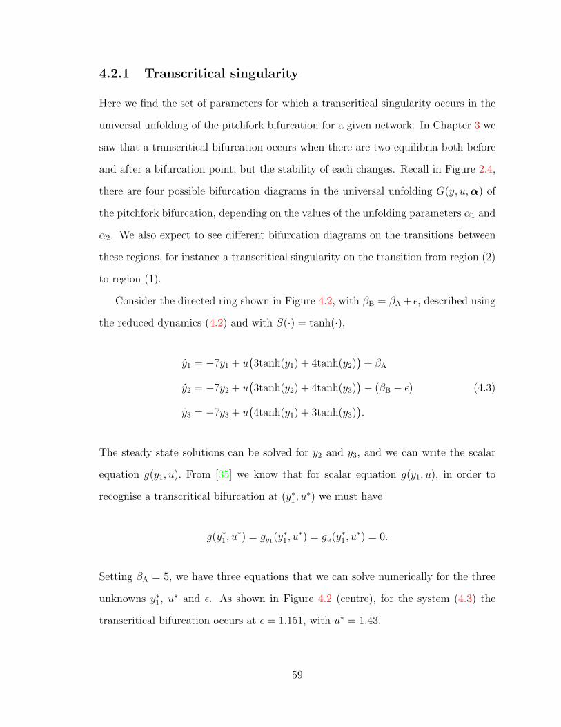
4.2.1 Transcritical singularity
Here we find the set of parameters for which a transcritical singularity occurs in the
universal unfolding of the pitchfork bifurcation for a given network. In Chapter 3 we
saw that a transcritical bifurcation occurs when there are two equilibria both before
and after a bifurcation point, but the stability of each changes. Recall in Figure 2.4,
there are four possible bifurcation diagrams in the universal unfolding G(y, u,α) of
the pitchfork bifurcation, depending on the values of the unfolding parameters α1 and
α2. We also expect to see different bifurcation diagrams on the transitions between
these regions, for instance a transcritical singularity on the transition from region (2)
to region (1).
Consider the directed ring shown in Figure 4.2, with βB = βA + ε, described using
the reduced dynamics (4.2) and with S(·) = tanh(·),
y1 = −7y1 + u(3tanh(y1) + 4tanh(y2)
)+ βA
y2 = −7y2 + u(3tanh(y2) + 4tanh(y3)
)− (βB − ε) (4.3)
y3 = −7y3 + u(4tanh(y1) + 3tanh(y3)
).
The steady state solutions can be solved for y2 and y3, and we can write the scalar
equation g(y1, u). From [35] we know that for scalar equation g(y1, u), in order to
recognise a transcritical bifurcation at (y∗1, u∗) we must have
g(y∗1, u∗) = gy1(y
∗1, u
∗) = gu(y∗1, u
∗) = 0.
Setting βA = 5, we have three equations that we can solve numerically for the three
unknowns y∗1, u∗ and ε. As shown in Figure 4.2 (centre), for the system (4.3) the
transcritical bifurcation occurs at ε = 1.151, with u∗ = 1.43.
59

Figure 4.2: Bifurcation diagrams for the network shown, with βA = 5 and βB = βA−ε.Left: With ε = 1 there is an unfolding towards alternative A. Centre: At ε = 1.151there is a transcritical singularity in the universal unfolding. Right: With ε = 1.3there is an unfolding towards alternative B.
Bifurcation diagrams for ε < 1.151 and ε > 1.151 are shown in Figures 4.2 (left)
and (right). The transcritical singularity occurs when the saddle node of Figure 4.2
(left) collides with the stable branch as ε increases. In Figure 4.2 (left) and (right) as
u increases from 1 to 2, the equilibrium varies smoothly and the trajectory does not
pass through the bifurcation point. The branch of the diagram corresponding to the
stable equilibrium for u = 1 remains stable for all u. In the transcritical bifurcation
diagram (Figure 4.2 (centre)), the branch that represents the stable equlibria for
u = 1 loses stability at the bifurcation point. The diagram in Figure 4.2 (centre) is
non-persistent, and we note that there are three equilibria before the bifurcation point
u∗. From a design perspective, the transcritical singularity represents a parameter
region in which the system is more sensitive to perturbations. When u− u∗ is small,
perturbations to the system could cause the trajectory of the average opinion y to
jump to the negative branch of the bifurcation diagram. This analysis also shows the
values of β at which the bifurcation diagram will change between regions of Figure 2.4.
60
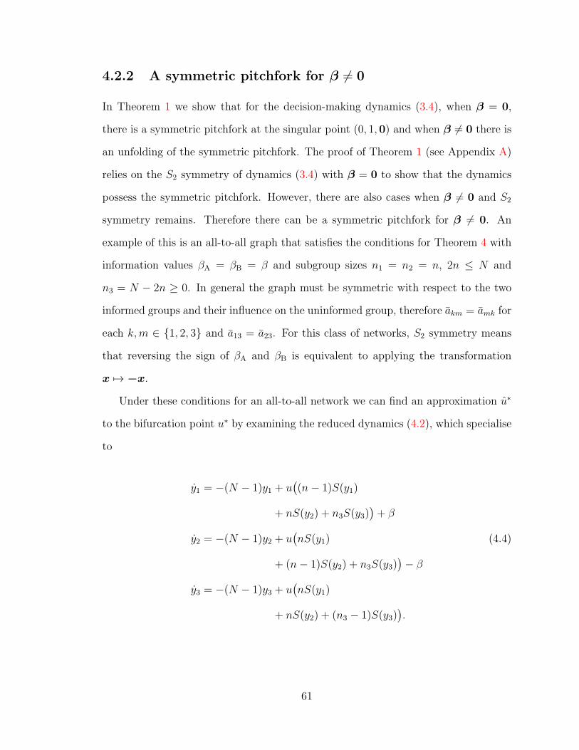
4.2.2 A symmetric pitchfork for β 6= 0
In Theorem 1 we show that for the decision-making dynamics (3.4), when β = 0,
there is a symmetric pitchfork at the singular point (0, 1,0) and when β 6= 0 there is
an unfolding of the symmetric pitchfork. The proof of Theorem 1 (see Appendix A)
relies on the S2 symmetry of dynamics (3.4) with β = 0 to show that the dynamics
possess the symmetric pitchfork. However, there are also cases when β 6= 0 and S2
symmetry remains. Therefore there can be a symmetric pitchfork for β 6= 0. An
example of this is an all-to-all graph that satisfies the conditions for Theorem 4 with
information values βA = βB = β and subgroup sizes n1 = n2 = n, 2n ≤ N and
n3 = N − 2n ≥ 0. In general the graph must be symmetric with respect to the two
informed groups and their influence on the uninformed group, therefore akm = amk for
each k,m ∈ {1, 2, 3} and a13 = a23. For this class of networks, S2 symmetry means
that reversing the sign of βA and βB is equivalent to applying the transformation
x 7→ −x.
Under these conditions for an all-to-all network we can find an approximation u∗
to the bifurcation point u∗ by examining the reduced dynamics (4.2), which specialise
to
y1 = −(N − 1)y1 + u((n− 1)S(y1)
+ nS(y2) + n3S(y3))
+ β
y2 = −(N − 1)y2 + u(nS(y1) (4.4)
+ (n− 1)S(y2) + n3S(y3))− β
y3 = −(N − 1)y3 + u(nS(y1)
+ nS(y2) + (n3 − 1)S(y3)).
61
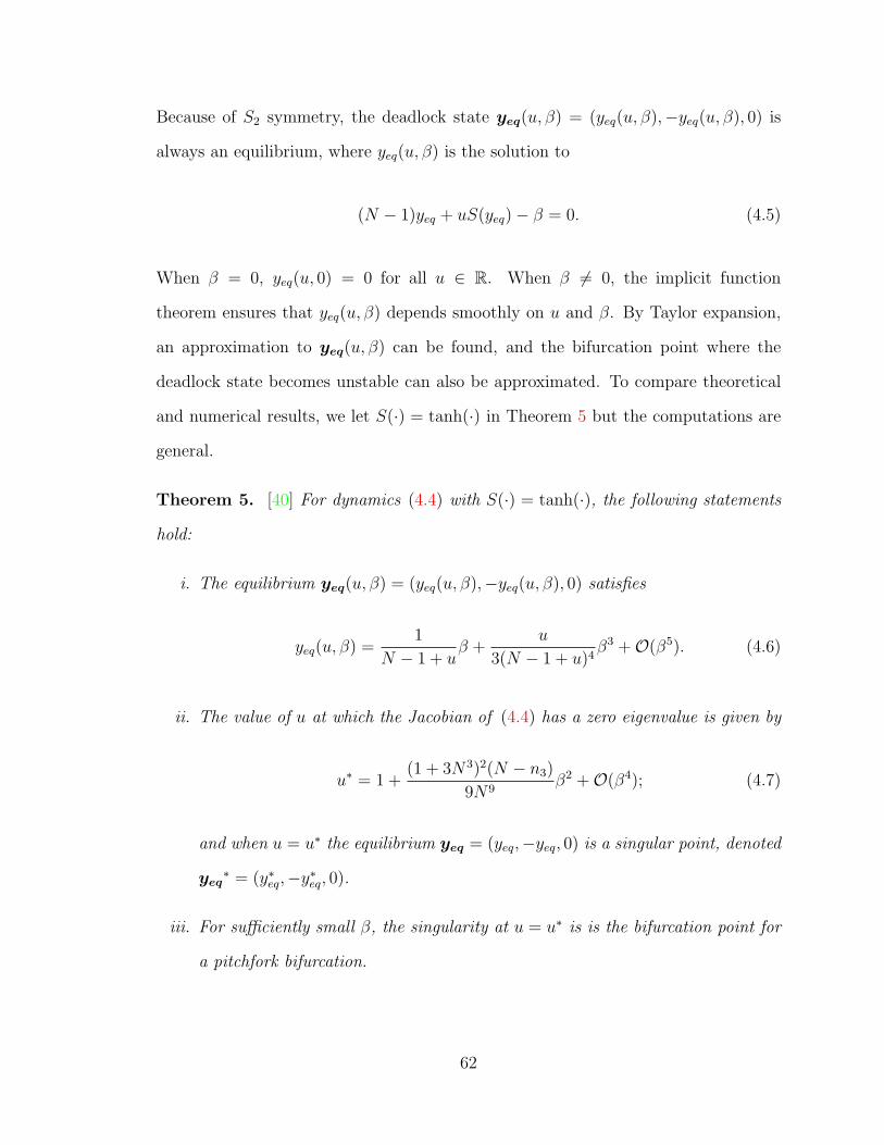
Because of S2 symmetry, the deadlock state yeq(u, β) = (yeq(u, β),−yeq(u, β), 0) is
always an equilibrium, where yeq(u, β) is the solution to
(N − 1)yeq + uS(yeq)− β = 0. (4.5)
When β = 0, yeq(u, 0) = 0 for all u ∈ R. When β 6= 0, the implicit function
theorem ensures that yeq(u, β) depends smoothly on u and β. By Taylor expansion,
an approximation to yeq(u, β) can be found, and the bifurcation point where the
deadlock state becomes unstable can also be approximated. To compare theoretical
and numerical results, we let S(·) = tanh(·) in Theorem 5 but the computations are
general.
Theorem 5. [40] For dynamics (4.4) with S(·) = tanh(·), the following statements
hold:
i. The equilibrium yeq(u, β) = (yeq(u, β),−yeq(u, β), 0) satisfies
yeq(u, β) =1
N − 1 + uβ +
u
3(N − 1 + u)4β3 +O(β5). (4.6)
ii. The value of u at which the Jacobian of (4.4) has a zero eigenvalue is given by
u∗ = 1 +(1 + 3N3)2(N − n3)
9N9β2 +O(β4); (4.7)
and when u = u∗ the equilibrium yeq = (yeq,−yeq, 0) is a singular point, denoted
yeq∗ = (y∗eq,−y∗eq, 0).
iii. For sufficiently small β, the singularity at u = u∗ is is the bifurcation point for
a pitchfork bifurcation.
62

Proof of Theorem 5. We begin with (i). Consider the Taylor series expansion of
yeq(u, β) with respect to β:
yeq(u, β) = βyI + β2yII + β3yIII + β4yIV +O(β5). (4.8)
Substitute (4.8) for yeq(u, β) into (4.5) and differentiate with respect to β to get
(N − 1)yeq′(u, β) + usech2
(yeq(u, β)
)yeq′(u, β)− 1 = 0.
Letting β = 0 yields yI = 1N−1+u
. Proceeding similarly for higher order deriva-
tives gives yII = yIV = 0 and yIII = u3(N−1+u)4
. Substituting these values into (4.8)
yields (4.6), establishing (i).
At the singular point u∗, the Jacobian of (4.4) computed at yeq∗ has a zero
eigenvalue, and the Jacobian drops rank. The Jacobian of (4.4) at yeq∗ is
[ −(N−1)+u(n−1)S′(y∗eq) unS′(y∗eq) un3
unS′(y∗eq) −(N−1)+u(n−1)S′(y∗eq) un3
unS′(y∗eq) unS′(y∗eq) −(N−1)+u(n3−1)
],
where we have used the fact that S ′(·) is an even function. For S(·) = tanh(·) the
determinant d of the Jacobian is
d = −1
4η(−1 +N + 2u+ ηcosh(2y1))(η + 3u+ n3u− 2Nu
− 2u2 + (η + u− n3u)cosh(2y1))sech4(y1),
with η = N − 1. A positive u = u∗ for which d = 0 satisfies
u∗ =1
4(3 + n3 − 2N + cosh(2y∗eq)− n3cosh(2y∗eq)
+√
16ηcosh2(y∗eq) + (3 + n3 − 2N − (−1 + n3)cosh2(2y∗eq])).
63

Note that y∗eq is also a function of u∗ and the above equation is a transcendental
equation in u∗, which can be solved numerically. To compute u∗ we use the Taylor
Series expansion u∗(β) = 1 + u∗Iβ + u∗IIβ2 + u∗IIIβ
3 +O(β4) and match coefficients to
obtain (4.7).
To prove that the singular point (yeq∗, u∗, β) corresponds to a pitchfork we in-
voke singularity theory for S2 symmetric bifurcation problems [35, Chapter VI]. By
Theorem 1, the singular point (yeq∗, u∗, β) is a pitchfork for β = 0. Because (4.4)
is S2 symmetric, for small β > 0 we obtain a small S2 symmetric perturbation of
the pitchfork at β = 0. Invoking genericity of the pitchfork in S2 symmetric sys-
tems [35, Theorem VI.5.1], we conclude that (4.4) possesses a pitchfork at u = u∗.
�
Theorem 5 shows that under the required symmetry conditions, the all-to-all net-
work possesses a symmetric pitchfork for β 6= 0. Additionally, we have approxima-
tions to the bifurcation point (yeq∗, u∗) that depend on the information value β, and
the sizes of the total group and uninformed subgroup (and implicitly the informed
subgroups). In the next section we use these expressions to analyse the effect of the
information value β and the group sizes n3 and N on the bifurcation point.
4.2.3 Value-sensitivity
In Chapter 2, Section 2.1 we discussed results from [69, 81] which showed how the
population-level model of the honeybee decision-making is value-sensitive. The criti-
cal level of stop-signalling required to break a deadlock between two equal alternatives
is inversely proportional to the value of those alternatives [69], which provides an as-
sociated sensitivity to environmental parameters, as discussed in Section 2.3.1. In
this section we demonstrate that dynamics (3.3), which are equivalent to our gener-
alised model (3.4) with time-scale change t = 1νs, recover the value-sensitivity of the
population-level model.
64
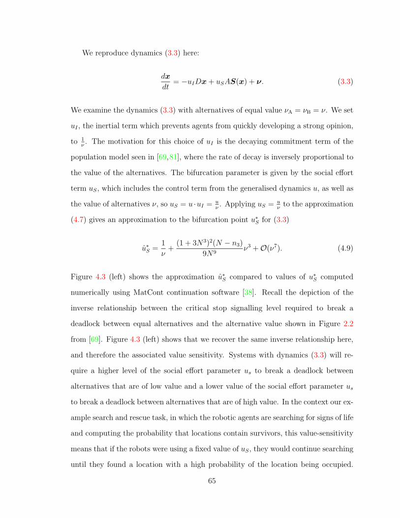
We reproduce dynamics (3.3) here:
dx
dt= −uIDx+ uSAS(x) + ν. (3.3)
We examine the dynamics (3.3) with alternatives of equal value νA = νB = ν. We set
uI , the inertial term which prevents agents from quickly developing a strong opinion,
to 1ν. The motivation for this choice of uI is the decaying commitment term of the
population model seen in [69,81], where the rate of decay is inversely proportional to
the value of the alternatives. The bifurcation parameter is given by the social effort
term uS, which includes the control term from the generalised dynamics u, as well as
the value of alternatives ν, so uS = u ·uI = uν. Applying uS = u
νto the approximation
(4.7) gives an approximation to the bifurcation point u∗S for (3.3)
u∗S =1
ν+
(1 + 3N3)2(N − n3)
9N9ν3 +O(ν7). (4.9)
Figure 4.3 (left) shows the approximation u∗S compared to values of u∗S computed
numerically using MatCont continuation software [38]. Recall the depiction of the
inverse relationship between the critical stop signalling level required to break a
deadlock between equal alternatives and the alternative value shown in Figure 2.2
from [69]. Figure 4.3 (left) shows that we recover the same inverse relationship here,
and therefore the associated value sensitivity. Systems with dynamics (3.3) will re-
quire a higher level of the social effort parameter us to break a deadlock between
alternatives that are of low value and a lower value of the social effort parameter us
to break a deadlock between alternatives that are of high value. In the context our ex-
ample search and rescue task, in which the robotic agents are searching for signs of life
and computing the probability that locations contain survivors, this value-sensitivity
means that if the robots were using a fixed value of uS, they would continue searching
until they found a location with a high probability of the location being occupied.
65
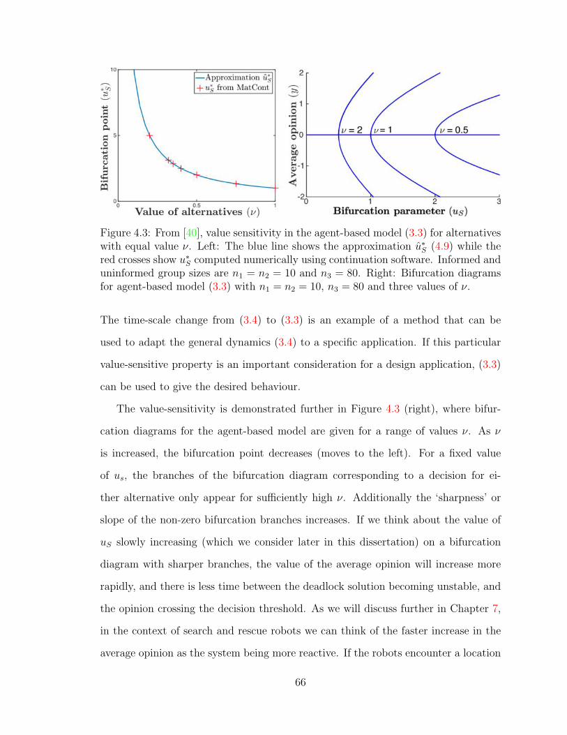
Figure 4.3: From [40], value sensitivity in the agent-based model (3.3) for alternativeswith equal value ν. Left: The blue line shows the approximation u∗S (4.9) while thered crosses show u∗S computed numerically using continuation software. Informed anduninformed group sizes are n1 = n2 = 10 and n3 = 80. Right: Bifurcation diagramsfor agent-based model (3.3) with n1 = n2 = 10, n3 = 80 and three values of ν.
The time-scale change from (3.4) to (3.3) is an example of a method that can be
used to adapt the general dynamics (3.4) to a specific application. If this particular
value-sensitive property is an important consideration for a design application, (3.3)
can be used to give the desired behaviour.
The value-sensitivity is demonstrated further in Figure 4.3 (right), where bifur-
cation diagrams for the agent-based model are given for a range of values ν. As ν
is increased, the bifurcation point decreases (moves to the left). For a fixed value
of us, the branches of the bifurcation diagram corresponding to a decision for ei-
ther alternative only appear for sufficiently high ν. Additionally the ‘sharpness’ or
slope of the non-zero bifurcation branches increases. If we think about the value of
uS slowly increasing (which we consider later in this dissertation) on a bifurcation
diagram with sharper branches, the value of the average opinion will increase more
rapidly, and there is less time between the deadlock solution becoming unstable, and
the opinion crossing the decision threshold. As we will discuss further in Chapter 7,
in the context of search and rescue robots we can think of the faster increase in the
average opinion as the system being more reactive. If the robots encounter a location
66

Figure 4.4: From [40], the inverse relationship between u∗S from (4.9) and the value ofthe equal alternatives ν in the agent-based model for three values of n3 with N = 7and n1 = n2 = N−n3
2.
with a very high probability of containing a survivor, they can move from indecision
to decision quickly, with only a small increase in the value of uS.
4.2.4 Influence of group size
An advantage of the agent-based framework is that it makes it possible to systemati-
cally study the sensitivity of the dynamics to model parameters including those that
describe network structure and heterogeneity. An examination of (4.9) shows that
u∗S decreases with increasing total group size N , implying that less social effort is
required to make a decision with a larger group. In the limit as N increases, u∗S → 1ν.
Figure 4.4 shows the inverse relationship between ν and u∗S for different values of
n3 with fixed N and n1 = n2 = N−n3
2. As n3 increases, the number of informed agents
decreases, and the curve drops, implying that increasing the number of uninformed
agents reduces the requirement on social effort to destabilise deadlock. We can also
think of decreasing the number of informed agents as decreasing the level of hetero-
geneity in the system. Recall from Chapter 2, Section 2.2, the results from [17, 60]
showed that adding uninformed individuals to a school of fish improved the ability
of the school to make decisions reliably. In particular, Leonard et al. showed in [60]
67
that increasing the number of uninformed individuals lowered the critical value of the
difference in preferred direction that was required for a decision to be made. The
findings of Leonard et al. are directly analogous to the relationship between n3 and
u∗ that we have found here, suggesting that our general dynamics (3.4) could also
be mapped to describe the dynamics of the schooling fish in [17, 60]. This analysis
directly addresses our design consideration of the effect of systems parameters on the
decision-making dynamics. When designing a multi-agent system that uses decision-
making dynamics (3.4), this result tells us that if we have a smaller total group, or a
larger number of agents collecting information about the environment, we will need
a higher level of social effort to break a deadlock. When we think about a group of
robots performing search and rescue, it is likely that one would want to maximise
the number of robots using sensing equipment in order to cover a large area, and this
would move the bifurcation point to the right, thereby making it harder to the group
to make a decision. In order to offset this effect, we could multiply each agent’s exter-
nal information value by some gain, which will move the bifurcation to the left. This
gain could be tuned depending on how many agents with are using sensing equipment.
4.2.5 Symmetric unfolding of pitchfork
We have now seen that under S2 symmetry, dynamics (3.4) possess a symmetric
pitchfork for β 6= 0. Additionally, when we map to dynamics (3.3), we see that the
approximation to the bifurcation point u∗S given by (4.9) is inversely proportional
to the value ν of the alternatives being considered. If we return to the generalised
dynamics (3.4) and the approximation to the bifurcation point u∗ of given by (4.7),
we see that the effect of increasing the value of the alternatives βA = βB = β is
to delay the bifurcation point, and for β > 0, u∗ > 1. Results from numerical
simulations of (3.4) showed a further effect of increasing the value of β; a transition
from the supercritical pitchfork, to a subcritical pitchfork and the emergence of two
68
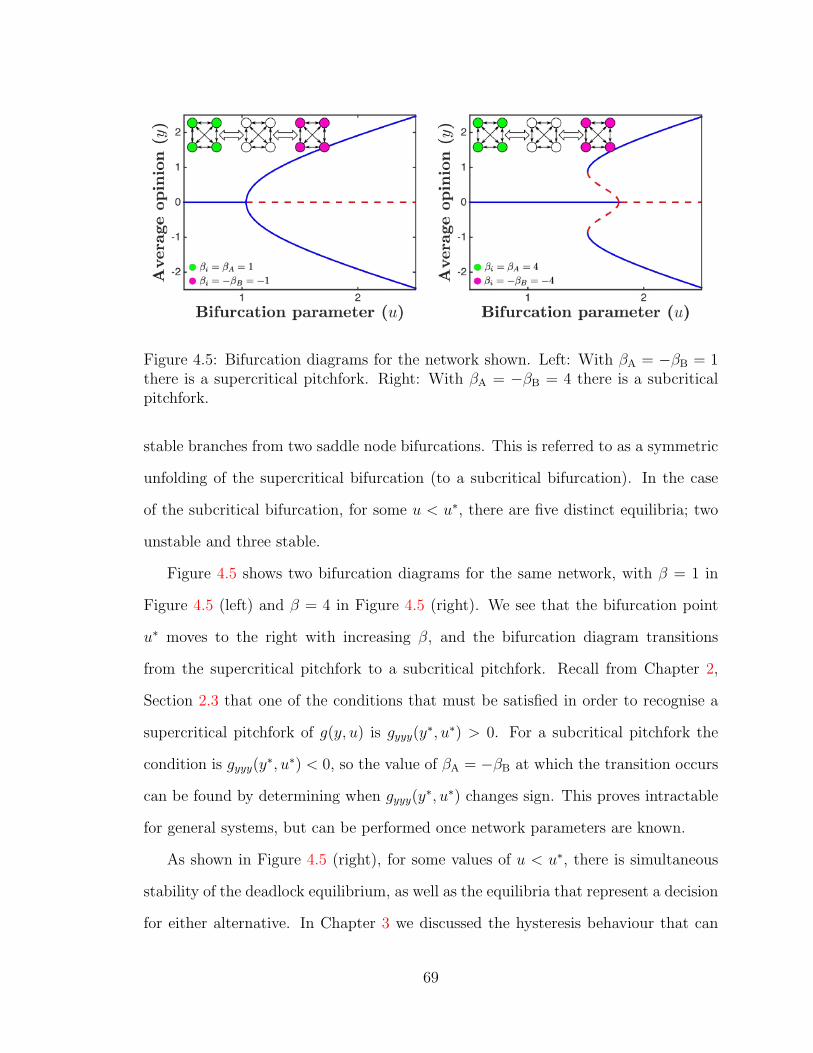
Figure 4.5: Bifurcation diagrams for the network shown. Left: With βA = −βB = 1there is a supercritical pitchfork. Right: With βA = −βB = 4 there is a subcriticalpitchfork.
stable branches from two saddle node bifurcations. This is referred to as a symmetric
unfolding of the supercritical bifurcation (to a subcritical bifurcation). In the case
of the subcritical bifurcation, for some u < u∗, there are five distinct equilibria; two
unstable and three stable.
Figure 4.5 shows two bifurcation diagrams for the same network, with β = 1 in
Figure 4.5 (left) and β = 4 in Figure 4.5 (right). We see that the bifurcation point
u∗ moves to the right with increasing β, and the bifurcation diagram transitions
from the supercritical pitchfork to a subcritical pitchfork. Recall from Chapter 2,
Section 2.3 that one of the conditions that must be satisfied in order to recognise a
supercritical pitchfork of g(y, u) is gyyy(y∗, u∗) > 0. For a subcritical pitchfork the
condition is gyyy(y∗, u∗) < 0, so the value of βA = −βB at which the transition occurs
can be found by determining when gyyy(y∗, u∗) changes sign. This proves intractable
for general systems, but can be performed once network parameters are known.
As shown in Figure 4.5 (right), for some values of u < u∗, there is simultaneous
stability of the deadlock equilibrium, as well as the equilibria that represent a decision
for either alternative. In Chapter 3 we discussed the hysteresis behaviour that can
69
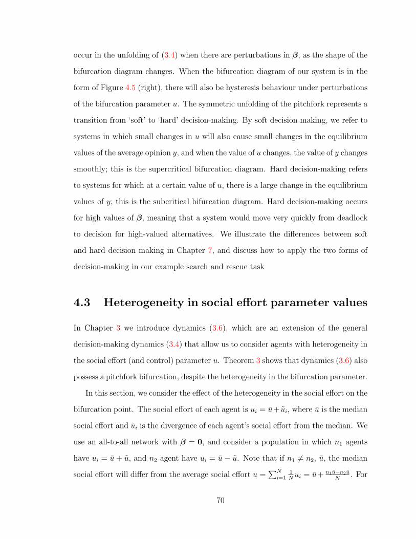
occur in the unfolding of (3.4) when there are perturbations in β, as the shape of the
bifurcation diagram changes. When the bifurcation diagram of our system is in the
form of Figure 4.5 (right), there will also be hysteresis behaviour under perturbations
of the bifurcation parameter u. The symmetric unfolding of the pitchfork represents a
transition from ‘soft’ to ‘hard’ decision-making. By soft decision making, we refer to
systems in which small changes in u will also cause small changes in the equilibrium
values of the average opinion y, and when the value of u changes, the value of y changes
smoothly; this is the supercritical bifurcation diagram. Hard decision-making refers
to systems for which at a certain value of u, there is a large change in the equilibrium
values of y; this is the subcritical bifurcation diagram. Hard decision-making occurs
for high values of β, meaning that a system would move very quickly from deadlock
to decision for high-valued alternatives. We illustrate the differences between soft
and hard decision making in Chapter 7, and discuss how to apply the two forms of
decision-making in our example search and rescue task
4.3 Heterogeneity in social effort parameter values
In Chapter 3 we introduce dynamics (3.6), which are an extension of the general
decision-making dynamics (3.4) that allow us to consider agents with heterogeneity in
the social effort (and control) parameter u. Theorem 3 shows that dynamics (3.6) also
possess a pitchfork bifurcation, despite the heterogeneity in the bifurcation parameter.
In this section, we consider the effect of the heterogeneity in the social effort on the
bifurcation point. The social effort of each agent is ui = u+ ui, where u is the median
social effort and ui is the divergence of each agent’s social effort from the median. We
use an all-to-all network with β = 0, and consider a population in which n1 agents
have ui = u + u, and n2 agent have ui = u− u. Note that if n1 6= n2, u, the median
social effort will differ from the average social effort u =∑N
i=11Nui = u+ n1u−n2u
N. For
70

n1 = n2, u = u. By adapting the reduction method above, we can reduce the system
in this case to two equations
x1 = −(N − 1)x1 + (u+ u)((n1 − 1)S(x1) + n2S(x2))
x2 = −(N − 1)x2 + (u− u)(n1S(x1) + (n2 − 1)S(x2)).
The heterogeneity in ui means that the agents in group 1 are paying more attention
to their neighbours (from both groups) while the agents in group 2 are paying less
attention. The nullclines of this system are given by
x1 =1
N − 1(u+ u)((n1 − 1)S(x1) + n2S(x2))
x2 =1
N − 1(u− u)(n1S(x1) + (n2 − 1)S(x2)),
and there are three solutions, (x1, x2) = {(0, 0), (+x∗1,+x∗2), (−x∗1,−x∗2)}. u ± u con-
trols the slope of the sigmoidal function S(·), so for small values of u±u, the nullclines
intersect only once at the origin, while for larger values there will be three intersec-
tions.
To find the value of u (as a function of u) at which the bifurcation occurs, we
consider the Jacobian of the system at the origin
J =
−(N − 1) + (n1 − 1)(u+ u) n2(u+ u)
n1(u− u) −(N − 1) + n2(u− u)
.The bifurcation point in terms u∗ is the value of u at which det(J) = 0. We know
n1 = N − n2, so u∗ is given by
u∗ = 1− N
2+
√u2 + u(2n2 −N) +
N2
4. (4.10)
71

Figure 4.6: The value of the bifurcation point u∗ in terms of the average u =∑N
i=11Nui
plotted against ui, for various sized groupings. Left: u =∑N
i=11Nui plotted against ui
for different total group sizes N , with n1 = n2. Right: u =∑N
i=11Nui plotted against
ui for a fixed N = 10, for various sizes of the group with reduced ui, n2.
The eigenvalues of J at (0, 0) are λ1,2 = −(N − 1)±√
(n1n2)(u2 − u2), so there are
two negative eigenvalues for u < u∗ and one positive and one negative eigenvalue for
u > u∗. For n1 = n2 = 1, (4.10) reduces to u∗ =√
1 + u2, and we see that the effect
of increasing u is to delay the bifurcation point, so higher social effort is required to
make a decision when there are higher inter-agent differences.
We can also study the effects of the group sizes n2 and N . In Figure 4.6 the value
of the bifurcation point in terms of the average social effort u =∑N
i=11Nui is plotted
against the size of ui, for various sized groupings. For Figure 4.6 (left) u∗ = u∗,
and we see that the delaying of the bifurcation point that occurs when we increase u
decreases with increasing group size N . In [60], Leonard et al. showed that increasing
the number of uninformed agents increases the parameter region in which a decision
is the only stable solution. We are not considering informed agents here, but we
do find that increasing the total group size leads to the same effect. In Figure 4.6
(right) we fix the total group size N , and consider different values of n1 and n2. The
bifurcation point is lowest for n2 = 1 and n2 = 9, so a decision is made with less social
effort when there are less agents with a different ui to the remainder of the group.
72

If our objective is to design a system with the lowest possible bifurcation point, we
should choose and large number of agents and minimise the level of heterogeneity in
the system.
In general, throughout this chapter we have seen that the effect of increasing the
level of heterogeneity of the group, such as through increasing the number of informed
agents or the difference in social effort values, is to delay the bifurcation point. The
result in Section 4.2.3, which showed that increasing the value of the alternatives
decreased the bifurcation point, is specific to dynamics (3.3) in time-scale t. For the
general dynamics (3.4) in time-scale s, which we consider for the majority of this
dissertation, increasing the value of the alternatives moves the bifurcation parameter
to the right. The location of the bifurcation parameter controls whether or not the
group reaches a decision, and is clearly an important parameter for the system. We
have shown that the effect of added heterogeneity is to delay the bifurcation point,
or move it to the right.
Returning to our example application; a search and rescue task occurs in an
emergency situation, so it is unlikely that operators of the system will be able to
make choices in terms of how many agents to use, and how to allocate sensors.
The results shown here demonstrate that by controlling the social effort value u,
an operator can ensure that the system reaches a decision when necessary, in spite
of parameters such as group size that they cannot control. The parameter u is a
powerful and simple way for the operator to interact with the system, a concept that
we will explore more in Chapters 6 and 7.
In this chapter we have used low-dimensional systems to explore the different
behaviours that we can expect from dynamics (3.4). We have shown that we recover
the value-sensitivity of the honeybee dynamics studied in [69, 81], as well as seeing
a similar improvement in decision-making abilities to those seen in [17, 60] when we
73

increase the total group size and decrease the level of heterogeneity in the system.
Although we cannot show that these results generalise to all networks, they provide
insight into the kinds of behaviour we can expect for general systems, and an example
of the types of analysis that can be performed once the system details are known.
In the next chapter we consider more general results that predict the effect of
asymmetry on the system, and also consider the performance of (3.4) in the presence
of noise.
74
Chapter 5
The symmetry-breaking effects of
agent preferences
In Chapter 2, Section 2.3, we saw that when asymmetry is introduced to a system
organised by a pitchfork bifurcation we see a qualitative change in the system be-
haviour, which we can characterise through unfolding theory [35]. In this chapter
we will consider the changes in behaviour due to asymmetry that arise when agents
have external information or prior preferences, and the β term of the decision-making
dynamics (3.4) is non-zero. We refer to the vector β as the information distribution.
We know that each βi ∈ {βA,−βB, 0}, and the information distribution tells us how
the values of βi are distributed amongst the group. As shown in Figure 4.5 if β 6= 0
but S2-symmetry is preserved the symmetry of the pitchfork bifurcation will persist,
and we see a symmetric unfolding to the subcritical pitchfork. However, this is a
special class of networks and information distribution, and we seek to understand
how external information will affect the dynamics generally, for any network and in
the absence of S2 symmetry.
75

We then consider decision-making in the presence of noise. We use the linearisation
of the nonlinear dynamics to predict the decision-making outcomes for a variety of
networks.
5.1 Results from singularity theory: eigenvector
centrality and βp
We begin by restating part (iii) of Theorem 1 from [40], given in full in Chapter 3;
“For β 6= 0, the solutions to g(y, u,β) = 0 undergo an N -parameter unfolding of
the symmetric pitchfork. Moreover, ∂g∂βi
(0, 1,0) = vT1 ei, where vT1 is the null left
eigenvector of L and ei is the i-th vector of the standard basis of RN”. This implies
that the influence of the external information βi of agent i on the reduced expression
g(y, u,β) is given by the ith element of the left eigenvector of the zero eigenvalue of
L, which we shall denote (vT1 )i.
Bonacich proposed the first left eigenvector of the largest eigenvalue of a network
as a centrality measure in [11], known as eigenvector centrality. A centrality measure
is a quantity that can be used to compare nodes in a graph in terms of their location
in the network, i.e., it defines a notion of how central a node is in a network. Cen-
trality measures have been used to describe the connection between the performance
outcomes of a network and the network structure. In [32], Freeman proposed the
intuitive notion that a centrality measure should always award the highest evaluation
to the central node of a star-shaped graph. An example of a centrality measure is
degree centrality ; the degree centrality of an agent in a network represented by an
unweighted graph is simply the number of its neighbours. Different problem formu-
lations and desired outcomes lead to different choices for measuring centrality. For
instance, for noisy networks, [71, 85] show how information centrality predicts the
ordering of nodes by certainty, while in [25] Fitch et al. define joint centrality and
76
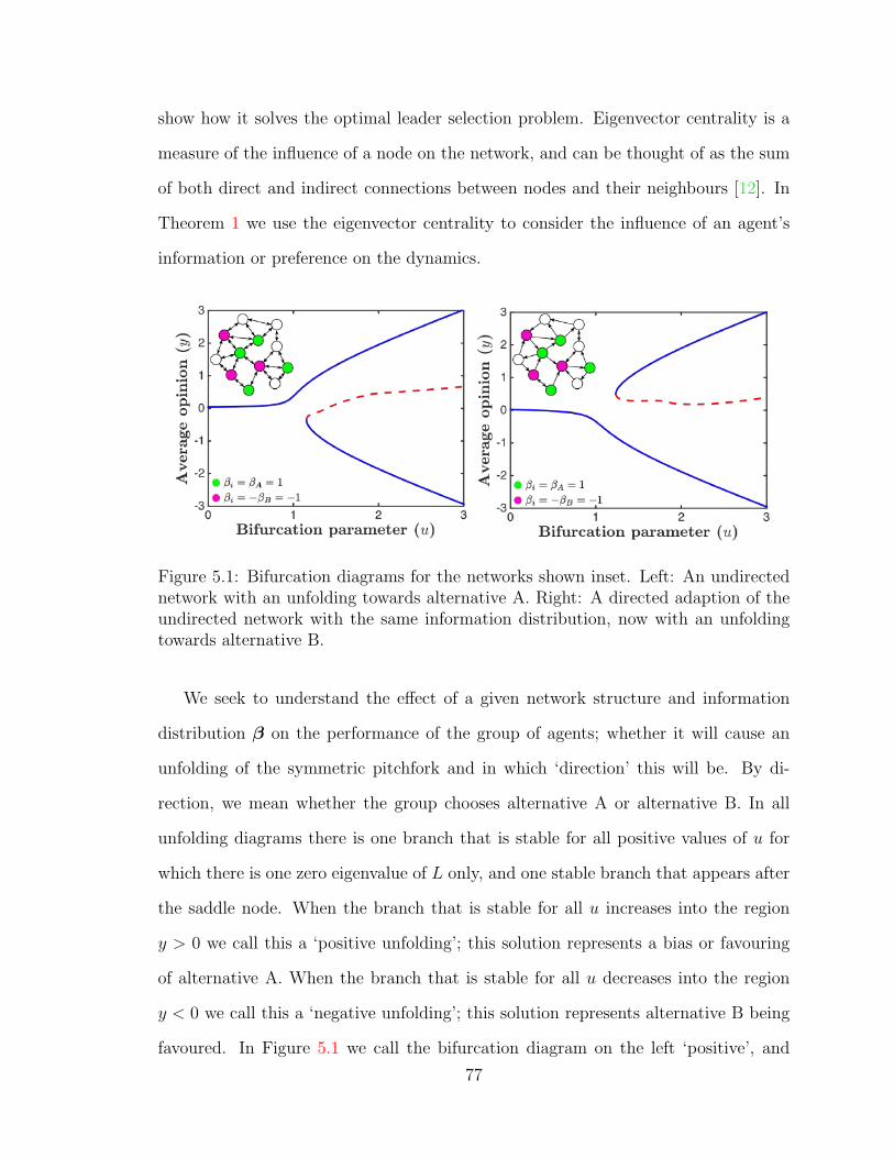
show how it solves the optimal leader selection problem. Eigenvector centrality is a
measure of the influence of a node on the network, and can be thought of as the sum
of both direct and indirect connections between nodes and their neighbours [12]. In
Theorem 1 we use the eigenvector centrality to consider the influence of an agent’s
information or preference on the dynamics.
Figure 5.1: Bifurcation diagrams for the networks shown inset. Left: An undirectednetwork with an unfolding towards alternative A. Right: A directed adaption of theundirected network with the same information distribution, now with an unfoldingtowards alternative B.
We seek to understand the effect of a given network structure and information
distribution β on the performance of the group of agents; whether it will cause an
unfolding of the symmetric pitchfork and in which ‘direction’ this will be. By di-
rection, we mean whether the group chooses alternative A or alternative B. In all
unfolding diagrams there is one branch that is stable for all positive values of u for
which there is one zero eigenvalue of L only, and one stable branch that appears after
the saddle node. When the branch that is stable for all u increases into the region
y > 0 we call this a ‘positive unfolding’; this solution represents a bias or favouring
of alternative A. When the branch that is stable for all u decreases into the region
y < 0 we call this a ‘negative unfolding’; this solution represents alternative B being
favoured. In Figure 5.1 we call the bifurcation diagram on the left ‘positive’, and
77

the diagram on the right ‘negative’. Understanding whether the bifurcation diagram
for a given system displays a positive or negative unfolding allows us to understand
which alternative the network is biased towards. These biases may be due to genuine
differences in the alternatives being considered, but also due to asymmetry associated
with how agents are located in the network. Developing an understanding of how the
various biases enter the system will improve our ability to design engineered systems;
for instance we can detect and remove unwanted biases.
Let us define
βp = vT1 β,
a scalar quantity that combines the eigenvector centrality with the information vector.
Because we associate alternatives A and B with positive and negative respectively,
we can use the sign of βp to predict the direction of the unfolding according to part
(iii) of Theorem 1 from [40]. When we discussed the universal unfolding of (3.4) in
Chapter 3, Subsection 3.2.3, we noted that our unfolding parameters β enter (3.4) and
the Lyapunov-Schmidt reduction g(y, u,β) of (3.4) linearly. In [35], Golubitksy et al.
show via the Lyapunov-Schmidt reduction that g = 〈vT1 ,f(x, u)〉 and ∂g∂βi
= 〈vT1 , ∂f∂βi 〉,
hence Theorem 1. Consequently, in the universal unfolding
G(y, u,α) = y3 − uy + α1 + α2y2, (2.4)
we conclude that this weighted combination of the information values βp = −α1
exactly. Returning to Figure 2.4 we see that for positive values of α1, and therefore
negative values of βp we see a negative unfolding, while for negative values of α1, and
therefore positive values of βp we see a positive unfolding.
Take, for instance, the networks shown in Figure 5.1. For Figure 5.1 (left), for the
network shown βp = 0.29, so βp > 0 and we predict an unfolding towards alternative
A. We can compare these results to the numerical results shown in Figure 5.1, which
78

indeed show a positive unfolding. For the network in Figure 5.1 (right), βp = −0.32,
so βp < 0 and, as predicted, we see an unfolding towards the negative alternative B.
The outcome in both cases is predicted correctly by the sign of βp.
Interestingly, both networks contain four nodes with a preference for A, and three
nodes for a preference for B. Intuitively we would expect A to be the preferred alter-
native in both cases, because there are more agents with this preference. However,
we see in Figure 5.1 (right) that alternative B, which is preferred by fewer agents, is
favoured. Clearly, the influence of the nodes with a preference for alternative B is
stronger. In Section 5.3 below we will revisit both networks and discuss the relative
influence of each agent.
5.1.1 Limitations of eigenvector centrality and βp
Theorem 1 addresses the bifurcation behaviour of the scalar equation g(y, u,β), which
is the Lyapunov-Schmidt reduction of our N -dimensional system (3.4). The results
of Theorem 1 show that for β = 0, dynamics (3.4) have S2 symmetry and undergo a
symmetric pitchfork bifurcation at the singularity (y∗, u∗). In Chapter 4 we showed
via Theorem 5 that a symmetric pitchfork also occurs for β 6= 0 when S2 symmetry
is preserved in the network structure and information distribution. If S2 symmetry is
not preserved, we see an unfolding of the pitchfork, and our aim is to understand how
and why this unfolding occurs. Developing a full understanding of how asymmetry
has entered the system is challenging, because there are many different ways in which
the S2 symmetry can be broken.
In the section prior we showed that for our system βp = −α1 in the universal
unfolding, and there is no dependence of α2 on β. α1 and α2 allow us to move
through all regions of Figure 2.4, so when considering the effect of β through the
present analysis, we can only move along one line in the parameter region. We
79

are therefore limited in our ability to study the unfolding behaviour, as there are
additional nonlinear, symmetry-breaking effects that we cannot describe analytically.
In Chapter 3, Section 3.1 we defined a balanced graph as a network for which the
in-degree and out-degree of each node are equal. For balanced graphs, just as every
row sums to zero so does every column, so vT1 = 1√N
1TN . Therefore, the eigenvector
centrality of each agent is equal. In this case, to the level that we have analysed,
there is symmetry between the agents and their influence on the network. Below,
we discuss cases in which the direction of unfolding for balanced graphs cannot be
predicted by the sign of βp, and we extend our analysis for some of these cases.
Recall in Figure 4.2 we considered a directed ring of subgroups of agents in which
the agents with a preference for alternative B have a direct influence on the unin-
formed agents, and the agents with a preference for alternative A do not. Each agent
has exactly seven neighbours, so it is a balanced network. When we set βA = 5 we
found that for βB < 3.849 (βp > 1.33) the unfolding was towards alternative A, and
for βB > 3.849 (βp < 1.33) the unfolding was towards alternative B. Therefore, the
sign of βp does not correctly predict the unfolding direction. For this balanced net-
work, the asymmetry in the graph that causes the unfolding behaviour is not captured
by the Lyapunov-Schmidt reduction and the subsequent analysis of Theorem 1.
Additionally, βp does not allow us to correctly predict the behaviour for the net-
works shown in Figure 5.2. In both cases βp = 0 which we would assume predicts
no unfolding, and the persistence of the symmetric bifurcation diagram. However, in
both cases we see an unfolding towards alternative B. There is an unfolding towards
the alternative preferred by the agents with more direct influence on the agents with
no preference.
Let us consider all balanced graphs with nA agents with βi = βA and nB agents
with βi = βB. Simulations show that if nA = nB, the left eigenvector centrality and
βp are not sufficient to predict the unfolding direction. There is symmetry in the
80
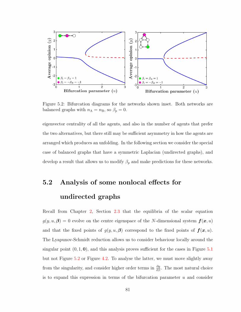
Figure 5.2: Bifurcation diagrams for the networks shown inset. Both networks arebalanced graphs with nA = nB, so βp = 0.
eigenvector centrality of all the agents, and also in the number of agents that prefer
the two alternatives, but there still may be sufficient asymmetry in how the agents are
arranged which produces an unfolding. In the following section we consider the special
case of balanced graphs that have a symmetric Laplacian (undirected graphs), and
develop a result that allows us to modify βp and make predictions for these networks.
5.2 Analysis of some nonlocal effects for
undirected graphs
Recall from Chapter 2, Section 2.3 that the equilibria of the scalar equation
g(y, u,β) = 0 evolve on the centre eigenspace of the N -dimensional system f(x, u)
and that the fixed points of g(y, u,β) correspond to the fixed points of f(x, u).
The Lyapunov-Schmidt reduction allows us to consider behaviour locally around the
singular point (0, 1,0), and this analysis proves sufficient for the cases in Figure 5.1
but not Figure 5.2 or Figure 4.2. To analyse the latter, we must move slightly away
from the singularity, and consider higher order terms in ∂g∂β
. The most natural choice
is to expand this expression in terms of the bifurcation parameter u and consider
81
values of u slightly above u = 1. Expanding ∂g∂β
at u = 1 gives
∂g
∂β(u) =
∂g
∂β
∣∣∣∣u=1
+d
du
(∂g
∂β
) ∣∣∣∣u=1
du. (5.1)
We know that ∂g∂β
∣∣u=1
= vT1 , so in order to find ddu
(∂g∂β
) ∣∣u=1
we seekdvT1du
∣∣u=1
. We
let L = D − uA, with L = L at u = 1, and consider how the first left eigenvector
of L perturbs for u > 1. We know balanced graphs have N linearly independent
eigenvectors that will perturb continuously with u, and the first eigenvalue λ1 and
associated left eigenvector vT1 must satisfy
vT1 (u)L(u) = vT1 (u)λ1(u).
To study how vT1 perturbs, we take the derivative with respect to u:
dvT1 (u)
duL(u)− vT1 (u)A =
dvT1 (u)
duλ1(u) + vT1 (u)
dλ1(u)
du.
At u = 1, λ1 = 0, and vT1 = 1TN , so
dvT1du
∣∣∣∣u=1
L− 1TNA = 1TNdλ1
du
∣∣∣∣u=1
dvT1du
∣∣∣∣u=1
= 1TN
(A+
dλ1
du
∣∣∣∣u=1
I
)L†, (5.2)
where L† is the pseudoinverse of L. Let us define the row vectors
bT =dvT1du
∣∣∣∣u=1
and dT = (diag(D))T .
82

Here, dT is row vector with each element dTi corresponding to the degree of agent i.
Like L, the rows and columns of L† sum to 0, so 1TNL† = 0. Returning to (5.2)
bT = dTL†.
Additionally, assuming a strongly connected network, we can write L† as L† =
V TˆV , where V is a matrix with rows vT1 , ..., vTN , the left eigenvectors of L, and
Λ† is a diagonal matrix with Λ†11 = 0 and Λ†ii = 1λi
for i ∈ {2, ..., N}. Recall from
Chapter 3 that for strongly connected networks λi > 0 for i = 2, ..., N . Therefore
bT = dTV TˆV.
From this expression we can find an expression for bi in terms of the remaining 2, ..., N
eigenvalues and eigenvectors of L. This expression is
bTi =N∑j=2
vji
∑Nk=1 d
Tk vjk
λj.
In the previous section we defined
βp =∂g
∂β=
⟨vT1 , β
⟩.
With the analysis of this section we now define
βu(u) =∂g
∂β(u) =
⟨vT1 +
dvT1du
∣∣∣∣u=1
du, β
⟩=
⟨vT1 + (u− 1)bT , β
⟩
for small (u− 1). βu allows us to predict how the consensus manifold perturbs, and
thus the direction of the unfolding, for some cases in which βp fails.
83

Let us now return to the networks shown in Figures 5.2, for which βp = 0. For
Figure 5.2 (left) at u = 1.1, βu = −0.03, and the sign of βu correctly predicts the
unfolding towards alternative B. Similarly for Figure 5.2 (right), βu = −0.02. For
these networks, the sign of βu correctly predicts the unfolding direction.
Figure 5.3: Bifurcation diagrams for the systems shown inset. The network is identicalfor both diagrams, but the information distribution has been changed.
We show further how βu makes it possible to distinguish the effect of differences in
information distribution vectors, where βp fails to do so. In Figure 5.3, we consider the
same network from Figure 5.2 (left), but with two different information distributions.
We have already seen that βu is negative for Figure 5.3 (left), corresponding to an
unfolding towards alternative B. For Figure 5.3 (right) βu = 0 which correctly predicts
that there is no unfolding, as the symmetry is preserved to a higher order.
To illustrate further, let us return to the undirected network shown in Figure 5.1
(left), but with a different information distribution such that nA = nB. With βA = βB
(and βp = 0) the bifurcation diagram unfolds towards alternative A, which is predicted
by a value of βu = 0.0133 at u = 1.1. In Figure 5.4 we slowly increase βB, so
βB > βA. For βB = 1.01, βu = 0.0041 predicting an unfolding towards A, while
for βB = 1.02, βu = −0.0051 predicting an unfolding towards B. These results are
confirmed numerically in Figure 5.4. Here the change in sign of βu allows us to
84

Figure 5.4: Bifurcation diagrams for the networks shown inset.
predict when the direction of the unfolding changes as we vary βB, to a high degree
of accuracy.
The predictions from βu do not apply to Figure 4.2 however. For all three values
of βB depicted, βu = βp > 0, but clearly the direction of the unfolding changes. This
result is as expected, because the analysis of this section was developed for undirected
graphs, which have a symmetric Laplacian matrix. The shown network in Figure 4.2
is a directed graph, so the Laplacian is not symmetric.
5.3 Implications for design
From the above results and analysis, we now have the following guidelines for pre-
dicting which alternative will be favoured in an unfolding of the symmetric pitchfork:
(a) For non-balanced graphs, and balanced graphs with nA 6= nB, the direction of
the unfolding is predicted by sgn(βp).
(b) For undirected graphs that do not satisfy (a) (with nA = nB) the direction of
unfolding is predicted by sgn(βu(u)) for small (u− 1).
(c) For directed, balanced graphs with nA = nB our criteria do not predict the
unfolding.
85

Many networks are covered by (a) and (b), so we are in a powerful position to
predict the effect of information distribution and network structure on the decision-
making outcomes of a group that behaves according to our dynamic model.. If ‘fair-
ness’ is a consideration, and a design criteria of high importance is designing a system
that will maintain a symmetric pitchfork bifurcation for equal alternatives, we can
design networks that satisfy (a) and/or (b) with βp = βu = 0, so there is no bias
due to network structure. Given that many engineered systems will be operating in
uncertain environments it is unlikely that the high level of symmetry required for a
symmetric pitchfork will be maintained in all scenarios, but when designing a system
we can at least ensure that the asymmetry is not entering the system via means that
are preventable.
If we consider just the left eigenvector vT1 and also vT1 , we can develop an under-
standing of the most influential nodes in the network. In our motivating example of a
search and rescue task, we discussed that different agents may have different sensing
capabilities. In some cases there may be a difference in the quality of sensor that
each agent is equipped with, so some agents will receive more reliable data. vT1 and
vT1 show us which nodes are the most influential in the network, and to improve the
accuracy of the group, the agents with better sensors should be placed in these more
influential positions. We can use vT1 and vT1 to determine how to arrange the agents
in a communication network, based on sensor quality.
To provide some intuition into how the centrality measures vT1 and vT1 distinguish
the influence of the agents, consider the the networks from Figure 5.1, which are
reproduced in Figure 5.5 with the values of vT1 and vT1 indicated. In Figure 5.5 (left)
we show the undirected network. For u = 1, vT1 = 1√12
1N ≈ 0.291N . For u = 1.1,
(vT1 )i increases for agents 1 and 3-6, stays roughly the same for agents 2, 8 and 9 and
decreases for agents 7 and 10-12. Agents 6 and 9 both have the highest number of
neighbours (5), but the neighbours of 6 have more neighbours than the neighbours
86

Figure 5.5: Values of vT1 for the networks from Figure 5.1. Left: the network is incategory (b), so we consider vT1 . Right: the network is in category (a), so vT1 suffices.
of 9, and this is reflected in vT1 . Eigenvector centrality considers both the direct and
indirect influence of an agent on its neighbours, hence the difference between agents
6 and 9.
In Figure 5.5 (right) there is a much larger inter-agent variation in the values of
vT1 . The most influential agent is agent 1, and the least influential is agent 11. Recall
from Figure 5.1 (right), agents 4, 6, 10 and 11 had a preference for alternative A and
agents 3, 8 and 9 for alternative B. Now that we have examined the values of vT1 , we
can easily see why alternative B was preferred by the group, as agents 3 and 9 have
a larger influence than all other informed agents.
5.4 Decision-making in the presence of noise
We now move to consider the network decision-making dynamics (3.4) in the presence
of uncertainty. We will also encounter a noisy system in Chapter 7, when we perform
experiments with robotic agents. Uncertainty or noise can enter the system through
the inter-agent communication channels or the sensing of external information. Suc-
cessful performance in the flexibility-stability trade-off requires sufficient robustness
to reject this uncertainty, while still remaining sensitive to system parameters. Suc-
cessful performance can be defined in a number of ways, for instance [43, 93, 94]
87
consider the robustness of consensus under uncertainty, and [71,72] study the contri-
bution of each agent to the overall uncertainty. For our system, we will consider the
performance of the group average, and the outcome of the group decision as defined
in Chapter 3.
To consider uncertainty we will use additive noise, and assume a zero mean and
independent and uncorrelated noise for each agent. The dynamics (3.4) become
dx = (−Dx+ uAS(x) + β)dt+ σdWN(t), (5.3)
where σ is the diffusion rate, which is homogeneous for all agents and WN(t) is the
standard N -dimensional vector of Weiner processes, which represents the additive
noise. We have only briefly defined these new terms here, but in the following subsec-
tion we will develop further understanding. Analysis of the noisy nonlinear dynamics
proves largely intractable, but like the deterministic nonlinear dynamics, these noisy
dynamics were designed around the linear consensus dynamics, and we can use anal-
ysis of the noisy linear system to make predictions for this nonlinear system. In the
next subsection we introduce the drift-diffusion model and Ornstein-Uhlbeck process,
which are the stochastic linear systems on which this (5.3) is based. We first present
the associated theory for these models, and then perform analysis that allows us to
predict the decision-making outcomes in the presence of noise for the linear dynamics,
and the nonlinear dynamics by extension.
5.4.1 The linearised, stochastic model
The linearisation of the noisy model at u = 1 is the drift-diffusion model (DDM),
which is often applied to the study of human performance in free-response two-
alternative choice tasks [10, 74, 75]. A free-response task is one in which there is
no time limit on making the decision, and a two-alternative choice task is a decision
88
between alternatives A and B, as in our nonlinear model. Many other forms of two-
alternative choice models can be shown to be equivalent to the DDM under optimal
parameter conditions [10]. The DDM models the integration over time of evidence
for the two alternatives, and a decision is made when the evidence crosses one of two
thresholds ±η. For a single agent, the DDM is
dx(t) = βdt+ σdW1(t). (5.4)
Here β is the drift rate, and the sign of β drives x towards ±η, while σ is the diffusion
rate, which scales the effects of the random noise simulated by the Weiner process
W1. Here E[W1(t)] = 0 and E[W1(t)2] = t. Results are given in [10] for how the
choice of β, σ and η values affect the dynamics and decision results. The DDM for a
network of agents with network Laplacian L is given by
dx(t) = (β − Lx(t))dt+ σdWN(t), (5.5)
so we see the drift term is modified to include the effects of an agent’s neighbours.
Prior analysis of the linear-stochastic model
In [83,84] Srivastava et al. used principal component analysis to separate the network
DDM into the principal component xp(t) = 1√NvT1 x(t) and the residual components
ε(t) = x(t)− xp(t)1N . The dynamics for these components are
dxp(t) = βpdt+ σdW1(t)
dε(t) =((β − βp1N)− Lε(t)
)dt+ σ(IN − v1v
T1 )dWN(t),
where IN is the N × N identity matrix and βp = 1√NvT1 β = 1√
Nβp. Recalling that
the first eigenvalue of L, λ1 = 0, they showed that the expected value and variance
89

of the principal component satisfy
E[xp(t)] = limλ1→0
βpλ1
(1− e−λ1t) = βpt
Var[xp(t)] = limλ1→0
σ2
2λ1
(1− e−2λ1t) = σ2t.
We see that the outcome of the centralised component depends on βp = 1√NvT1 β, a
scaling of the product of the eigenvector centrality and external preference vector.
Additionally, in [83], Srivasatava et al. discussed the speed-accuracy trade-off. This
is analogous to the flexibility-stability trade-off discussed in this thesis, but seeking
to balance decision-making performance that will favour a quick decision or a highly
accurate one. They showed that performance in this trade-off depends on the selection
of the threshold η.
Considering u > 1
Thus far we have considered the linearisation of the nonlinear model at u = 1 only.
We now wish to consider values of u > 1, so we introduce the Ornstein-Uhlbeck
process [15]
dx(t) = (β − Lx(t))dt+ σdWN(t). (5.6)
As in Section 5.2, we let L = D − uA to consider values of u > 1. The eigenvalues
and left eigenvectors of L are denoted λTi and vi respectively. For u > 1, λ1 > 0,
and we restrict ourselves to values of u ∈ [1,Ψ) for which λ1 is the only non-positive
eigenvalue. The condition on u for which there is only one non-positive eigenvalue
was found in [26], with
u <1
λn−1(D−1A)= Ψ,
90

where λn−1(D−1A) is the second largest eigenvalue of the matrix D−1A. When u = 1,
L = L. (5.6) is a mean-reverting model: over time the process drifts towards some
mean value.
5.4.2 Analysis of the linear-stochastic dynamics
The analysis of [83, 84] considered the central component xp(t) = 1√NvT1 x(t), but we
wish to consider the performance of the group average y(t) = 1N
∑Ni=1 xi(t), which
differs from xp(t) when (vT1 )i 6= (vT1 )j ∀ i 6= j with i, j ∈ {1, ..., N}. We consider all
graphs for which the network Laplacian L and the adapted form L are diagonalisable,
and therefore have N linearly independent left eigenvectors.
Theorem 6. For dynamics (5.5), with information vector β and L diagonalisable,
we define V , a matrix with rows vT1 , ..., vTN , the left eigenvectors of L.
i. The expected value of the average opinion y(t) is given by
E[y(t)] ≈ g11βp
−λ1
e−λ1t
where βp = vT1 β and g11 = 1N
1TN V−1∗1 . V −1
∗1 is the first column of V −1. We know
g11 > 0 and −λ1 > 0, so sgn(E[y(t)]
)= sgn(βp).
ii. For u = 1, this reduces to
E[y(t)] ≈ g11βpt,
iii. and for balanced graphs at u = 1
E[y(t)] =βp√Nt.
91

Proof of Theorem 6.
(i) L is diagonalisable so we can write L = V −1ΛV , where V is a matrix with
rows vT1 , ..., vTN , the left eigenvectors of L and Λ is a diagonal matrix of the associated
eigenvalues. We define the change of coordinates
x =
x1
x2
...
xN
→ z =
y
x2
...
xN
where y(t) = 1
N1TNx(t). The transformation matrix z(t) = Tx(t) is therefore
T =
1n
1n
1n
. . . 1n
0 1 0 . . . 0
0 0 1 . . . 0
......
.... . .
...
0 0 0 . . . 1
,
so dz = Tdx. Applying this change of coordinates to (5.5) we may write
dz(t) = (Tβ − TLT−1z(t))dt+ TσdW n(t).
The expected value of z(t) is given by
E[z(t)] =
∫ t
0
e−T LT−1τTβdτ
=
∫ t
0
Te−Lτβdτ
=
∫ t
0
T V −1e−Λτ V βdτ. (5.7)
92

We are interested in E[y(t)], which is the first entry of (5.7), and we let
Ge−Λτ = T V −1e−Λτ .
For large t, the 2,...,N entries of the first row of matrix Ge−Λτ will decay quickly to
zero as 0 < λ2 < ... < λN . Therefore the first entry g11e−λτ will dominate and we can
write
E[y(t)] ≈∫ t
0
g11e−λ1tvT1 βdτ
≈ g11βp
−λ1
e−λ1t.
We know that g11,−λ1 > 0, so the sign of the expected value of y and therefore the
expected alternative chosen are determined by βp.
(ii) For u = 1 we have L = L and λ1 = 0, and in this case e−Λτ is a diagonal
matrix with (e−Λτ )11 = 1. The 2,...,N entries will decay to zero, so
E[y(t)] ≈∫ t
0
g11vT1 βdτ
≈ g11βpt.
(iii) The eigenvectors vT2 , ...,vTN are all orthogonal to vT1 which is 1√
N1TN for bal-
anced graphs, so the first row of TV −1 is [ 1√N, 0, ..., 0], and we can therefore write the
first entry of (5.7) exactly as
E[y(t)] =βp√Nt. �
Theorem 6 shows that, as in the deterministic nonlinear case, we can use the sign
of βp to predict how the network structure and information distribution will affect
the outcome of the decision for the linear-stochastic dynamics. Unlike the previous
93

analysis in Section 5.2, where βp was a local result around the singularity (0, 1,0),
the analysis of this section allows us to consider behaviour for u > 1 via βp. The
changes in vT1 with u are incorporated in the result, and our extension with βu is not
necessary. In the next section we will use results from simulations to examine how
well this analysis of the noisy linear dynamics allows us to predict the results of the
noisy nonlinear dynamics (5.3).
5.5 Results for the linear and nonlinear models
with noise.
We now perform Monte Carlo simulations on the noisy nonlinear system (5.3), to
demonstrate how the results of Theorem 6 for the linearised system predict the
decision-making outcomes of the nonlinear system in the presence of noise. Fig-
ure 5.6 shows results for a variety of networks that we have discussed throughout this
chapter. Each simulation advances dynamics (5.3) with the parameter values shown
until the average opinion of the group of agents being considered crosses one of the
two decision thresholds ±η. We performed 5000 simulations for each data point, over
u ∈ [1.5, 4] and in all simulations the decision threshold η = 1, and the diffusion
rate σ = 0.2. When the average opinion of the group crosses η = 1 we say that the
group has chosen alternative A, and when it crosses η = −1 we say that the group
has chosen alternative B. The initial opinion of each agent xi(0) = 0 for all trials.
To guarantee that a decision was made in reasonable time, we used values of u that
correspond to |y(t)| > |η| on the bifurcation diagrams of the networks. In each trial
we recorded whether alternative A or B was chosen, and then for each value of u we
found the percentage of trials for which the alternative chosen was predicted by the
sign of βp.
94

Figure 5.6: Results of the Monte Carlo simulations of dynamics (5.3) for Networks 1- 5 shown. In all simulations σ = 0.2 and η = ±1.
The values of η and σ naturally affect the results of the decision, and these could
be optimised to improve the accuracy and speed of decision-making. Our interest is
in how well the sign of βp predicts which alternative is chosen by the group, so we do
not consider the affects of our choices for these parameters.
95

In the first set of simulations, in Figures 5.6 (top, left and right) we set βA = 1.5
and βB = 1. For all networks, this means βp > 0 (shown in Figure 5.6 (top, left)) so
we expect the network to choose alternative A by crossing the positive threshold. As
shown in Figure 5.6 (top, right) for u = 1.5 the groups chose alternative A in > 80%
of the trials. Network 1 is the closest to 100% accurate, as nA > nB, so there is a
bias for alternative A both in the values of β, and the number of agents with that
preference. Generally we see an overall correlation between the magnitude of |βp|
for each network, and the level of accuracy across all u values. As u increases, the
accuracy for all networks declines. If we recall dynamics (5.3), we see that the drift
rate of each agent is affected by the agent’s preference value βi as well as the opinions
of the agent’s neighbours. As u increases the influence of each agent’s neighbours
will increase relative to the value of its preference, so less importance is placed on
this information value. Notice that the performance of Networks 4 and 5 decays the
most. In Chapter 4 we discussed how increasing the total group size improved the
performance of the group by lowering the level of social effort u required to break
a deadlock between alternatives. Here we see that increasing the group size also
improves the ability of the group to reject disturbances in a noisy system.
Recall from Chapter 2, Figure 2.5, we showed that close to the bifurcation point, an
unfolding of the bifurcation diagram causes very different behaviour to the symmetric
pitchfork, while far away from the bifurcation point (u >> 1) the unfolded bifurcation
diagram remains similar to the symmetric diagram. As we increase u in Figure 5.6
(top, right) we move to a part of the bifurcation diagram where the bias due to the
different β values is less prevalent, and this is likely why the percentage of times
that the result is predicted by βp decreases. In all simulations here, the value of u
was constant during each simulation, so for higher values of u, the system did not
come close to the highly sensitive bifurcation point. There is only one branch of the
bifurcation diagram that is stable for u < 1, so if a simulation is begun with u < 1
96

and the value of u is increased, the equilibrium of that system will remain on that
stable branch and move in the direction of that unfolding. Here for simulations with
large u we did not move through the bifurcation point, but began already past it, so
the system does not benefit from the high sensitivity around the bifurcation point.
High values of u may be advantageous to force a system to make a decision quickly,
but in order to remain highly sensitive to system parameters the value of u should
be slowly raised from u < 1. In the next chapter we design an adaptive feedback
dynamic which does exactly this.
In the second set of simulations, shown in Figures 5.6 (bottom), we set βA =
βB = 1, so here we consider the effect of asymmetry due to the network structure
and information distribution rather than information value. For an all-to-all network,
with nA = nB, we would expect each alternative to be chosen 50% of the time because
the system is symmetric, but here we consider networks that introduce asymmetry. In
the deterministic case these networks cause an unfolding of the symmetric pitchfork,
and a bias towards one of the two alternatives.
For Network 1 nA > nB and βp > 0, therefore we predict that alternative A
would be chosen. This prediction is correct > 60% of the time, but less often than
in the first set of simulations. In the first set, nA > nB and βA > βB. For the
first set of simulations the value of the external information in the expression for the
average opinion y is 0.75, while in the second set the value is 0.25. The value of the
diffusion rate is 0.2, which is much closer to the value of the external information in
the expression for y in the second set of simulations, so it is harder for the system to
distinguish between the noise and the external information.
The percentage of times that either alternative is chosen is close to 50% for Net-
works 2-4. These are cases where nA = nB, so the noise seems to inhibit some of
the bias that appears due to the asymmetric information distribution. Given than
βA = βB, we can consider the bias in the networks due to asymmetrical network struc-
97

ture as an unwanted effect. The addition of noise appears to counteract the sources
of bias, and we see results close to what we would expect for a symmetric pitchfork
bifurcation. Note that nA = nB for Network 5 also but there is more apparent bias.
This could be due to the fact that there are fewer uninformed agents, or fewer agents
overall. We discussed above how increasing the number of agents in a network im-
proves the performance, and if we interpret the removal of bias as an advantage, we
observe a similar improvement with increasing group size here.
The results of this chapter can be applied to several of our six design consider-
ations, and therefore aid design choices. We again saw that the influence of system
parameters, particularly the total group size, improves the performance of the system.
Also, the eigenvector centrality vT1 and adapted vector vT1 provide an understanding
of the role of the network structure. In our search and rescue example this result
would inform where in a communication network to place robots with higher quality
sensors. Finally, the results of this last section demonstrated the sensitivity close to
the bifurcation point, and robustness far away from the bifurcation point that we
have discussed as an important result for the flexibility-stability trade-off. In the
next chapter, where we design an adaptive feedback dynamic, we must ensure that
our dynamics allow the trajectory to pass through the region around the bifurcation
point in order to remain sensitive to environmental parameters.
98

Chapter 6
Adaptive dynamics to ensure a
decision
In this chapter we design a decentralised adaptive feedback dynamic that increases
the value of u, the bifurcation parameter and social effort level, until the magnitude of
the average opinion |y| of a group of agents reaches some set threshold. u is increased
slowly, so that the dynamics move through the region close to the bifurcation point,
thus ensuring that we retain the high level of sensitivity that occurs in this parameter
region. We present a feedback algorithm that can be implemented by a group of agents
with or without external information, and with any strongly connected network. The
work in this chapter was originally presented in [40]. I was the co-lead contributor to
the section relevant to this chapter along with Alessio Franci, who wrote the version
of Theorem 7 that appeared in [40]. Vaibhav Srivastava and Naomi Ehrich Leonard
provided oversight and guidance. The writing and results presented here are a revision
of the work presented in [40], and provide a more thorough presentation. Theorem
7 has also been revised. In Section 6.2 we reference a video that implements the
proposed feedback dynamics with a robotic system. The video was created for [48] a
99

Princeton University senior thesis written by Sofi Inglessis, with guidance from myself
and Naomi Ehrich Leonard. The video was created by Sofi Inglessis and myself.
6.1 Design objectives
In the previous chapters we have seen how the network topology and system param-
eters influence the behaviour of systems with the decision-making dynamics (3.4), by
altering the underlying bifurcation diagram. For instance, we know that increasing
the value of the alternatives being considered will delay the bifurcation point for dy-
namics (3.4) with bifurcation parameter u, and make the bifurcation appear earlier
for dynamics (3.3) with bifurcation parameter uS. In this chapter we consider the
network topology and the system parameters to be characteristics determined exter-
nally, i.e., by the environment. In our example setting of a search and rescue task, the
agents will be sensing values of β as they explore the environment, and the network
topology may change depending on the availability of communication. The range and
values of β and disruptions to the communication will not be known ahead of time,
but the group must still be able to make a decision. We wish to design feedback
dynamics which can ensure that a group of autonomous agents will be able to make
a decision in any set of environmental conditions.
Recall from the introduction to the model in Chapter 3, we defined a decision as
occurring when the magnitude of the steady state value average opinion |y| is greater
than a threshold η and when all the opinion of all agents has the same sign, which is
the case when the disagreement δ = |yss| − 1N‖xss‖1 = 0. In order to ensure that a
decision is made, we must ensure that |y| crosses the threshold, and the agent opinions
remain sufficiently close to the average. The value of u at which the stable branches of
the bifurcation diagram and therefore |y| will cross η depend on the network topology
and system parameters, and how they alter the bifurcation diagram.
100

In the literature, typical objectives in control of nonlinear systems that exhibit
bifurcation behaviour involve controlling characteristics of the bifurcation diagram.
For instance, in [90], Wang et al. delay the onset of an inherent bifurcation and
introduce a new bifurcation, while in [1,2], Abed et al. stabilise a bifurcated solution
or branch. For our system, the shape of the bifurcation diagram should remain
unconstrained and free to respond to the environmental conditions, as this is what
provides system sensitivity. Therefore we seek to change the value of u without
affecting the behaviour of the underlying bifurcation. Additionally, we saw in the
previous chapter how systems that begin deliberating with u > u∗ (the bifurcation
point) do not have the same sensitivity as systems with u close to u∗. The dynamics
on u must begin at u < u∗ and increase u slowly to allow the trajectory to pass
through the region around the singularity.
The parameter u was inspired by the inhibitory stop-signalling performed by hon-
eybees during their nest-site selection process. As shown in [69,81], when the bees are
considering equal alternatives, the level of stop-signalling required to break a dead-
lock between alternatives is sensitive to the value of the alternatives being considered.
Pais et al. postulated in [69] that the bees may increase the level of stop-signalling
during the decision-making process. The bees do not feed during the deliberation, so
over time they may feel an increased urgency to make a decision. We take inspiration
from this hypothesis here, and design dynamics that slowly increase u proportional to
the distance of the group average y from a threshold yth. yth could be set as equal to
the decision threshold η, or slightly higher to allow for disturbances. The dynamics
on u are
u = ε(y2th − y2) (6.1)
101
where ε is a small constant that ensures the dynamics are sufficiently slow. We begin
by considering a system in which each agent has identical u dynamics, and then
generalise to systems for which this is not the case, i.e., where the control is fully
decentralised.
6.2 Adaptive dynamics for an all-to-all network
with β = 0
In order to demonstrate the adaptive feedback dynamics and the associated theory,
we begin with an all-to-all network with β = 0. In an all-to-all network every agent
has access to every other agent’s opinions and therefore can calculate the average
opinion of the group y = 1N
∑Ni=1 xi. We consider an idealised case in which the
dynamics on the bifurcation parameter u are a function of the global parameters y,
yth and u(0) only, and each agent has identical u dynamics.
To design adaptive feedback dynamics for an all-to-all network with N uninformed
agents we modify dynamics (3.4) as follows:
x = −Dx+ uAS(x) (6.2a)
u = ε(y2th − y2). (6.2b)
We may use the centre manifold theorem [41, Theorem 3.2.1] to show that dynam-
ics (6.2) converge to a low-dimensional manifold. We augment (6.2) with a dummy
dynamic for ε, giving
x = −Dx+ uAS(x) (6.3a)
u = ε(y2th − y2), (6.3b)
ε = 0. (6.3c)
102
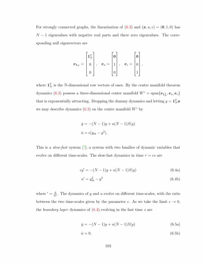
For strongly connected graphs, the linearisation of (6.3) and (x, u, ε) = (0, 1, 0) has
N − 1 eigenvalues with negative real parts and three zero eigenvalues. The corre-
sponding null eigenvectors are
e1N=
1TN
0
0
, eu =
0
1
0
, eε =
0
0
1
,
where 1TN is the N-dimensional row vectors of ones. By the centre manifold theorem
dynamics (6.3) possess a three-dimensional center manifold W c = span{e1TN, eu, eε}
that is exponentially attracting. Dropping the dummy dynamics and letting y = 1TNx
we may describe dynamics (6.3) on the centre manifold W c by
y = −(N − 1)y + u(N − 1)S(y)
u = ε(yth − y2).
This is a slow-fast system [7]; a system with two families of dynamic variables that
evolve on different time-scales. The slow-fast dynamics in time τ = εs are
εy′ = −(N − 1)y + u(N − 1)S(y) (6.4a)
u′ = y2th − y2 (6.4b)
where ′ = ddτ
. The dynamics of y and u evolve on different time-scales, with the ratio
between the two time-scales given by the parameter ε. As we take the limit ε → 0,
the boundary layer dynamics of (6.4) evolving in the fast time s are
y = −(N − 1)y + u(N − 1)S(y) (6.5a)
u = 0, (6.5b)
103

and the reduced dynamics evolving in the slow time τ are
0 = −y + uS(y) (6.6a)
u = y2th − y2. (6.6b)
These dynamics can be analysed using geometric singular perturbation theory from
[22], see [52, Chapters 1 & 2] for a review.
The reduced dynamics in slow time are defined on the slow manifold M =
{(y, u) | y = y(u)}, where y(u) is the solution to −y + uS(y) = 0. The manifold
is normally hyperbolic; the eigenvalues have non-zero real parts. The reduced dy-
namics (6.6) describe the behaviour of the system (6.2) close to the slow manifold
M, while the boundary layer dynamics (6.5) describe the behaviour far away from
M. At ε = 0 we can consider the two sets of dynamics separately, but this does not
allow us to understand the full behaviour of the system. Geometric singular pertur-
bation theory [22, 52] allows us to study both simultaneously, and requires that ε be
small but non-zero.
Fenichel theory [22], [52, Theorems 1 and 3] states that for small ε > 0, there
exists a manifoldMε that lies within O(ε) ofM. Mε is diffeomorphic toM, locally
invariant under dynamics (6.2) and Cr for r < ∞. Additionally, there exist stable
and unstable manifolds W s(Mε) and W u(Mε) that lie within O(ε) of W s(M) and
W u(M). The results of these theorems tell us that the flow of our adaptive feedback
system (6.2) remains (ε) close to the flow of (6.5a) for small ε.
For dynamics (6.2), from the above theory and Corollary 2, we know that for u < 1
the slow manifold M consists of one globally exponentially stable branch at y = 0,
and for u > 1 that branch becomes exponentially unstable and we see the appearance
of two locally exponentially stable branches at y = ±ys(u) where ys
S(ys)= u. The
104
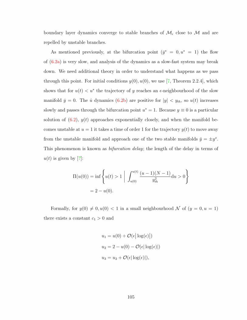
boundary layer dynamics converge to stable branches of Mε close to M and are
repelled by unstable branches.
As mentioned previously, at the bifurcation point (y∗ = 0, u∗ = 1) the flow
of (6.2a) is very slow, and analysis of the dynamics as a slow-fast system may break
down. We need additional theory in order to understand what happens as we pass
through this point. For initial conditions y(0), u(0), we use [7, Theorem 2.2.4], which
shows that for u(t) < u∗ the trajectory of y reaches an ε-neighbourhood of the slow
manifold y = 0. The u dynamics (6.2b) are positive for |y| < yth, so u(t) increases
slowly and passes through the bifurcation point u∗ = 1. Because y ≡ 0 is a particular
solution of (6.2), y(t) approaches exponentially closely, and when the manifold be-
comes unstable at u = 1 it takes a time of order 1 for the trajectory y(t) to move away
from the unstable manifold and approach one of the two stable manifolds y = ±ys.
This phenomenon is known as bifurcation delay ; the length of the delay in terms of
u(t) is given by [7]:
Π(u(0)) = inf
{u(t) > 1
∣∣∣∣ ∫ u(t)
u(0)
(u− 1)(N − 1)
y2th
du > 0
}
= 2− u(0).
Formally, for y(0) 6= 0, u(0) < 1 in a small neighbourhood N of (y = 0, u = 1)
there exists a constant c1 > 0 and
u1 = u(0) +O(ε∣∣ log(ε)
∣∣)u2 = 2− u(0)−O(ε| log(ε)|)
u3 = u2 +O(ε| log(ε)|),
105

such that
0 ≤ y(t) ≤ ε for u1 ≤ u(t) ≤ u2
|y(t)| − ys(u) ≤ c1ε for u(t) ≥ u3,
for all times t such that (y(t), x(t)) ∈ N . See [7, Theorem 2.2.4] for the full theorem
and proof. This theorem describes how the trajectory (y(t), u(t)) converges to the
deadlock equilibrium y = 0 for u(0) < 1, slides along it past the bifurcation point and
then after a delay (until u(t) > 2−u(0)) converges to one of the two stable branches.
We can now describe the trajectory y(t) under the adaptive dynamics (6.2).
Finally, it remains to show that the dynamics converge to |y(t)| = yth. By inspec-
tion of dynamics (6.2b), we see that for |y(t)| < yth, u > 0 and for |y| > yth, u < 0.
The dynamics (6.2b) drive u to increase until |y| reaches the threshold value yth.
Therefore the adaptive feedback ensures a group of agents with dynamics (6.2) will
make a decision for yth > η.
Figure 6.1: Bifurcation diagram and sample trajectory for a group of 12 agents withdynamics (6.2), with ε = 0.01.
Figure 6.1 shows the bifurcation diagram and trajectory for an all-to-all system
of 12 agents with dynamics 6.2, threshold yth = 2 and ε = 0.01. The bifurcation
diagram is shown with the stable branches in blue and the unstable branch in red,
106

while the trajectory for (y(t), u(t)) is shown in purple. The trajectory begins at the
initial conditions (y(0), u(0)) and as |y(t)| < yth, u > 0. As u(t) increases from u(0)
to u1, y(t) approaches ±ε of the stable branch y = 0. u(t) continues to increase and
passes through the bifurcation point u∗ = 1, but due to the bifurcation delay effect,
y(t) remains within ε of the now unstable branch y = 0 until u(t) = u2. As u(t)
increases from u2 to u3, y(t) approaches ±ε of the positive stable branches y = ys.
For u(t) > u3, y(t) increases along the stable branch until y(t) = yth.
Thus we have, for a special case, shown that with the addition of adaptive feed-
back to decision-making dynamics (3.4), the behaviour of the group average y of the
adapted system (6.2a) remains close to the behaviour of the original system (3.4).
The effect of the feedback (6.2b) is to increase the social effort term u, until the
group average y has reached a (positive or negative) threshold and therefore can en-
sure that the group has made a decision. Note that whether y crosses the positive
or negative threshold, i.e. chooses alternative A or B, will depend on initial con-
ditions and no agent in the group will know in advance which alternative will be
chosen. Because the consensus manifold x = y1N is globally attracting, these re-
sults hold globally. The dynamics (6.2) are demonstrated in a video, which can be
found at https://youtu.be/6ismnvwTmjc [48]. There are several screenshots below
in Figure 6.2.
In the top left frame of Figure 6.2, u(t) ≈ u0, and the robots are at their initial
positions, with y(0) 6= 0. In the top right frame u(t) ≈ u1, and the robots have
converged close to the stable equilibrium y = 0. In the bottom left frame u(t) ≈ u2,
and the value of u(t) has passed beyond the bifurcation point and the equilibrium
y = 0 has become unstable. We see that the yellow spot in the light strip have
moved away from y = 0 but the robots remain at this location due to the bifurcation
delay. In the bottom right frame u(t) ≈ u3 and the robots have ‘caught up’ to the
equilibrium value, and we say that a decision has been made. The robotic system
107

Figure 6.2: Screenshots from a video made with Sofi Inglessis [48]. The video can befound at https://youtu.be/6ismnvwTmjc. The robots implement dynamics (6.2).Each robot represents an agent so N = 3. The colour of the light strips under eachrobot represents the current value of u (see the bottom of each frame for a key). Theyellow spots represent the stable values of y∗ for the current value of u. The videoillustrates the bifurcation delay, as the yellow lights representing y∗ move away fromy = 0 before the robots do (see the bottom left frame denoted u2).
used in the demonstration is very simple, with very little uncertainty, but in more
complex systems the adaptive feedback allows us to ensure that a decision is made
by an autonomous system. The group of robots has the flexibility to choose which
alternative to decide for, and no external interaction with the system is required.
In Figure 6.3 we plot the trajectory of the group average y for dynamics (6.2) for
two groups of different sizes. The teal line represents a small group with N = 12,
while the purple line represents a larger group with N = 50. Both networks had the
same initial control value u(0). We see that the bifurcation delay for the larger group
is much smaller. The bifurcation delay occurs because the trajectories approach the
deadlock solution y = 0 very closely, so even after the bifurcation point has been
crossed, it takes time for the flow to grow large enough for the trajectory to move
108

Figure 6.3: Bifurcation diagram and trajectories of the average group opinion for twoall-to-all networks with β = 0.
away from y = 0. With a larger group, the higher number of agents seem to develop
enough ‘momentum’ to move the trajectory away from the deadlock sooner. The
effect of group size is not captured in the bound on the bifurcation delay Π(u(0), so
we may consider this effect part of the error O(ε|log(ε)|). In Figure 6.1, ε = 0.05, so
ε|log(ε)| ≈ 0.35, which accounts for the difference in delay lengths of the trajectories.
Throughout this thesis, we have seen benefits in system performance that result from
an increase in total group size. We saw in Chapter 4 that larger groups of decision-
making agents can lead to a decrease in the value of the bifurcation point u∗ and
in [18], Couzin et al. found that larger groups require proportionally less informed
agents to ensure that the correct alternative is chosen by the group. Here we see that
there is a shorter delay as the trajectory of the group moves through the bifurcation
point. From a design perspective, there are certainly benefits to designing systems
with a larger group of agents.
109
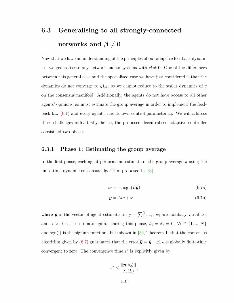
6.3 Generalising to all strongly-connected
networks and β 6= 0
Now that we have an understanding of the principles of our adaptive feedback dynam-
ics, we generalise to any network and to systems with β 6= 0. One of the differences
between this general case and the specialised case we have just considered is that the
dynamics do not converge to y1N , so we cannot reduce to the scalar dynamics of y
on the consensus manifold. Additionally, the agents do not have access to all other
agents’ opinions, so must estimate the group average in order to implement the feed-
back law (6.1) and every agent i has its own control parameter ui. We will address
these challenges individually, hence, the proposed decentralised adaptive controller
consists of two phases.
6.3.1 Phase 1: Estimating the group average
In the first phase, each agent performs an estimate of the group average y using the
finite-time dynamic consensus algorithm proposed in [34]
w = −αsgn(Ly) (6.7a)
y = Lw + x, (6.7b)
where y is the vector of agent estimates of y =∑N
i=1 xi, wi are auxiliary variables,
and α > 0 is the estimator gain. During this phase, ui = xi = 0, ∀i ∈ {1, ..., N}
and sgn(·) is the signum function. It is shown in [34, Theorem 1] that the consensus
algorithm given by (6.7) guarantees that the error y = y−y1N is globally finite-time
convergent to zero. The convergence time s∗ is explicitly given by
s∗ ≤ ||y(s0)||λ2(L)
,
110
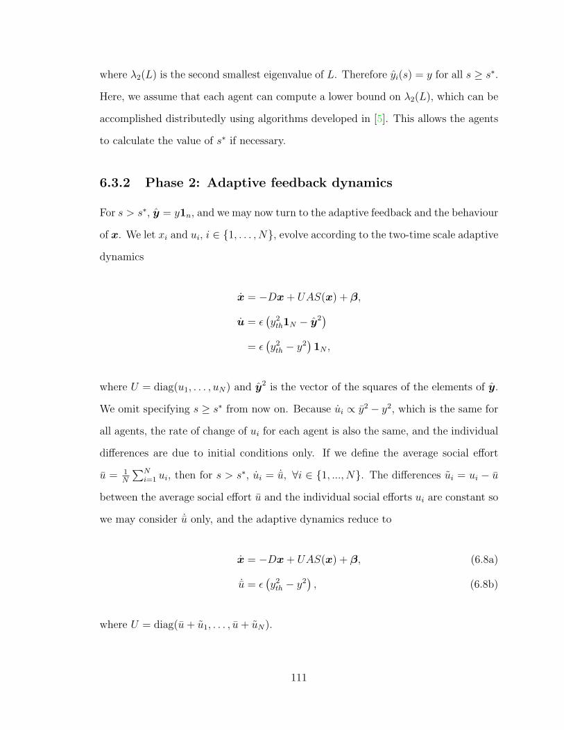
where λ2(L) is the second smallest eigenvalue of L. Therefore yi(s) = y for all s ≥ s∗.
Here, we assume that each agent can compute a lower bound on λ2(L), which can be
accomplished distributedly using algorithms developed in [5]. This allows the agents
to calculate the value of s∗ if necessary.
6.3.2 Phase 2: Adaptive feedback dynamics
For s > s∗, y = y1n, and we may now turn to the adaptive feedback and the behaviour
of x. We let xi and ui, i ∈ {1, . . . , N}, evolve according to the two-time scale adaptive
dynamics
x = −Dx+ UAS(x) + β,
u = ε(y2th1N − y2
)= ε
(y2th − y2
)1N ,
where U = diag(u1, . . . , uN) and y2 is the vector of the squares of the elements of y.
We omit specifying s ≥ s∗ from now on. Because ui ∝ y2 − y2, which is the same for
all agents, the rate of change of ui for each agent is also the same, and the individual
differences are due to initial conditions only. If we define the average social effort
u = 1N
∑Ni=1 ui, then for s > s∗, ui = ˙u, ∀i ∈ {1, ..., N}. The differences ui = ui − u
between the average social effort u and the individual social efforts ui are constant so
we may consider ˙u only, and the adaptive dynamics reduce to
x = −Dx+ UAS(x) + β, (6.8a)
˙u = ε(y2th − y2
), (6.8b)
where U = diag(u+ u1, . . . , u+ uN).
111

As discussed previously, the dynamics of x do not converge to y1N , so instead
we must find a suitable low-dimensional invariant manifold for (6.8) by means of the
centre manifold theorem [41, Theorem 3.2.1]. To use the centre manifold computation
we extend (6.8) with dummy dynamics for ε and β [91, Section 18.2]:
x = −Dx+ UAS(x) + β, (6.9a)
˙u = ε(y2th − y2
), (6.9b)
ε = 0, (6.9c)
β = 0. (6.9d)
By Theorem 3, if the graph is strongly connected, the linearisation of (6.9) at
(x, u, ε,β) = (0, u∗(u), 0,0) has N − 1 eigenvalues with negative real part and 3 +N
zero eigenvalues, with corresponding null eigenvectors
evTN =
vTN
0
0
0
, eu =
0
1
0
0
, eε =
0
0
1
0
, eβ,i
0
0
0
ei
, i = 1, ..., N,
where vN is defined in Theorem 3 as the right null eigenvector of the linearisation
of the dynamics (3.6). ei is the i-th vector of the standard basis of RN . It follows
by the centre manifold theorem, that (6.9) possesses an (N + 3)-dimensional centre
manifold W c = span{evTN , eu, eε, eβ,i, i = 1, ..., N} that is exponentially attracting.
112
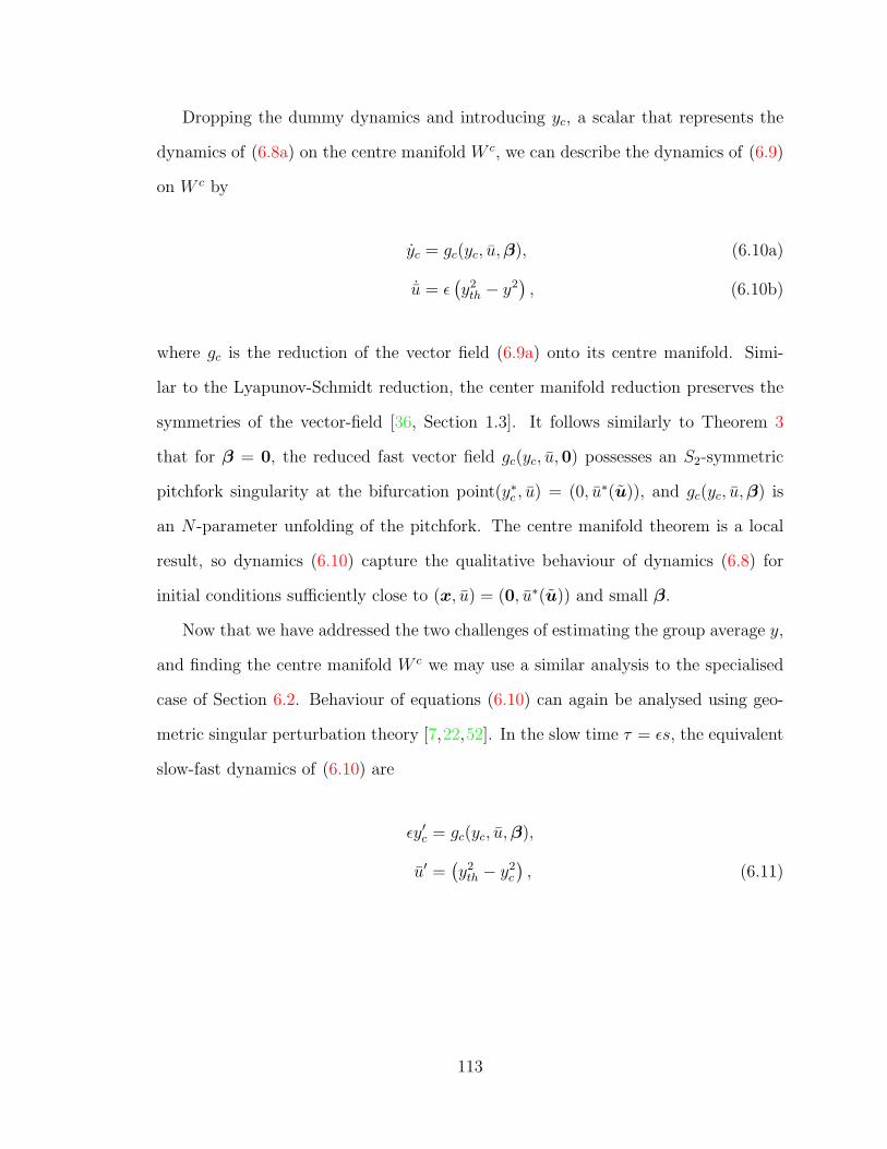
Dropping the dummy dynamics and introducing yc, a scalar that represents the
dynamics of (6.8a) on the centre manifold W c, we can describe the dynamics of (6.9)
on W c by
yc = gc(yc, u,β), (6.10a)
˙u = ε(y2th − y2
), (6.10b)
where gc is the reduction of the vector field (6.9a) onto its centre manifold. Simi-
lar to the Lyapunov-Schmidt reduction, the center manifold reduction preserves the
symmetries of the vector-field [36, Section 1.3]. It follows similarly to Theorem 3
that for β = 0, the reduced fast vector field gc(yc, u,0) possesses an S2-symmetric
pitchfork singularity at the bifurcation point(y∗c , u) = (0, u∗(u)), and gc(yc, u,β) is
an N -parameter unfolding of the pitchfork. The centre manifold theorem is a local
result, so dynamics (6.10) capture the qualitative behaviour of dynamics (6.8) for
initial conditions sufficiently close to (x, u) = (0, u∗(u)) and small β.
Now that we have addressed the two challenges of estimating the group average y,
and finding the centre manifold W c we may use a similar analysis to the specialised
case of Section 6.2. Behaviour of equations (6.10) can again be analysed using geo-
metric singular perturbation theory [7,22,52]. In the slow time τ = εs, the equivalent
slow-fast dynamics of (6.10) are
εy′c = gc(yc, u,β),
u′ =(y2th − y2
c
), (6.11)
113
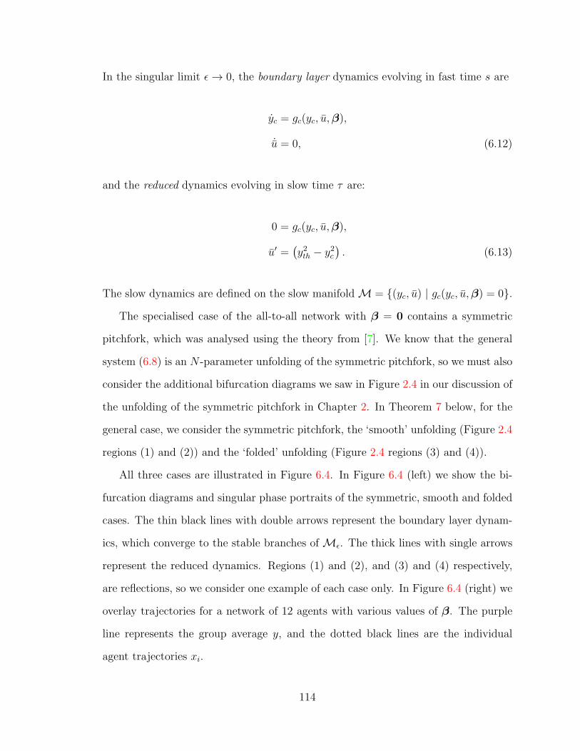
In the singular limit ε→ 0, the boundary layer dynamics evolving in fast time s are
yc = gc(yc, u,β),
˙u = 0, (6.12)
and the reduced dynamics evolving in slow time τ are:
0 = gc(yc, u,β),
u′ =(y2th − y2
c
). (6.13)
The slow dynamics are defined on the slow manifoldM = {(yc, u) | gc(yc, u,β) = 0}.
The specialised case of the all-to-all network with β = 0 contains a symmetric
pitchfork, which was analysed using the theory from [7]. We know that the general
system (6.8) is an N -parameter unfolding of the symmetric pitchfork, so we must also
consider the additional bifurcation diagrams we saw in Figure 2.4 in our discussion of
the unfolding of the symmetric pitchfork in Chapter 2. In Theorem 7 below, for the
general case, we consider the symmetric pitchfork, the ‘smooth’ unfolding (Figure 2.4
regions (1) and (2)) and the ‘folded’ unfolding (Figure 2.4 regions (3) and (4)).
All three cases are illustrated in Figure 6.4. In Figure 6.4 (left) we show the bi-
furcation diagrams and singular phase portraits of the symmetric, smooth and folded
cases. The thin black lines with double arrows represent the boundary layer dynam-
ics, which converge to the stable branches of Mε. The thick lines with single arrows
represent the reduced dynamics. Regions (1) and (2), and (3) and (4) respectively,
are reflections, so we consider one example of each case only. In Figure 6.4 (right) we
overlay trajectories for a network of 12 agents with various values of β. The purple
line represents the group average y, and the dotted black lines are the individual
agent trajectories xi.
114
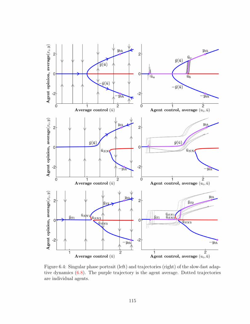
Figure 6.4: Singular phase portrait (left) and trajectories (right) of the slow-fast adap-tive dynamics (6.8). The purple trajectory is the agent average. Dotted trajectoriesare individual agents.
115

Theorem 7. For dynamics (6.10), with a strongly connected interconnection network,
there exists ε > 0 such that, for all ε ∈ (0, ε] and all yth > 0, the following hold.
i. Case 1: Symmetric Pitchfork, shown in Figure 6.4 (top). For all initial con-
ditions yc(0), u(0) in a small neighbourhood N of ((y∗, < u∗(u)) such that
|yc(0)| > 0 is sufficiently small, 0 < u(0) < u∗(u), and |u(0) − u∗(u)| suffi-
ciently small, let us define
a(yc, u) =dgcdyc
Π(u(0)) = inf
{u(t) > u∗
∣∣∣∣ ∫ u(t)
u(0)
a(y∗, u)
y2th
du > 0
}.
There exists a constant c1 > 0 and
ua = u(0) +O(ε∣∣ log(ε)
∣∣)ub = Π(u(0))−O(ε| log(ε)|)
uc = ub +O(ε| log(ε)|),
such that
0 ≤ yc(t) ≤ ε for ua ≤ u(t) ≤ ub
|yc(t)− y(u)| ≤ c1ε for u(t) ≥ uc,
for all times t such that (yc(t), u(t)) ∈ N . For u ≥ uc and |yc(t)| < yth, the
trajectory of (6.10) slides along the stable branch ±y(u) until |y(t)| = yth.
ii. Case 2: ‘Smooth’ Unfolding, shown in Figure 6.4 (middle). For all initial con-
ditions yc(0), u(0) such that |yc(0)| > 0 is sufficiently small, 0 < u(0) < u∗(u),
and |u(0)− u∗(u)| sufficiently small, the trajectory of (6.10) exponentially ap-
116
proaches the manifold y(u) at u = u(0) + O(ε∣∣ log(ε)
∣∣), and slides along y(u)
with ˙u > 0 until |y(t)| = yth.
iii. Case 3: ‘Folded’ Unfolding, shown in Figure 6.4 (bottom). Note that there are
two saddle node bifurcations at (ySN1, uSN1) and (ySN2, uSN2). For all initial
conditions yc(0), u(0) such that |yc(0)| > 0 is sufficiently small, 0 < u(0) <
u∗SN1, and |u(0)− u∗SN1| sufficiently small, there exist constants c1, c2, c3 and c4
such that
|yc(t)− yS1| ≤ c1ε
u(t)for u(0) ≤ u(t) ≤ uSN2 − c2ε
23
|yc(t)− ySN2| ≤ c3ε13 for uSN2 − c2ε
23 ≤ u(t) ≤ uSN2 + c4ε
23 .
yc(t) then approaches yS2 and slides along it until yc(t) = yth.
Proof of Theorem 7
i. Case 1: For all times such that u(t) ≤ uc, the behaviour of the trajectory follows
exactly from [7, Theorem 2.2.4]. The behaviour of the trajectory is exactly as
described for the all-to-all network in section 6.2 with the appropriate constants
given above, and with the exceptions that the consensus manifold y is replaced
by the centre manifold yc. For u(t) ≥ uc we note that for |yc(t)| < yth, ˙u > 0,
so yc(t) increases until |yc(t)| = yth.
ii. Case 2: The smooth branch of the bifurcation diagram is normally hyperbolic
and attracting, so the behaviour of the trajectory follows directly from Fenichel
theory [22], [52, Theorems 1,3]. That is, the trajectory approaches the smooth
branch y(u) of the slow manifoldM for u > u(0)+O(ε∣∣ log(ε)
∣∣), ˙u > 0. There is
no bifurcation point between the ‘deadlock’ region with y(u) close to 0, and the
‘decision’ region with y(u) close to yth, so yc(t) slides along the smooth branch
until |yc(t)| = yth.
117
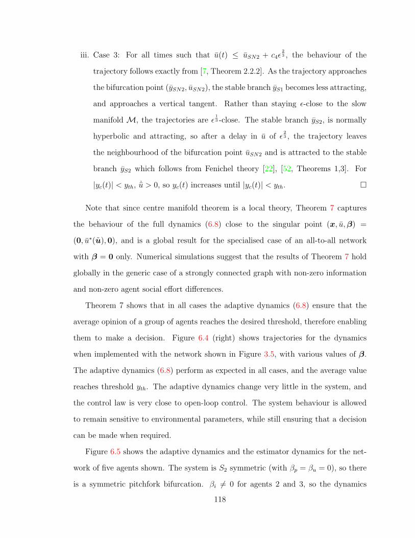
iii. Case 3: For all times such that u(t) ≤ uSN2 + c4ε23 , the behaviour of the
trajectory follows exactly from [7, Theorem 2.2.2]. As the trajectory approaches
the bifurcation point (ySN2, uSN2), the stable branch yS1 becomes less attracting,
and approaches a vertical tangent. Rather than staying ε-close to the slow
manifold M, the trajectories are ε13 -close. The stable branch yS2, is normally
hyperbolic and attracting, so after a delay in u of ε23 , the trajectory leaves
the neighbourhood of the bifurcation point uSN2 and is attracted to the stable
branch yS2 which follows from Fenichel theory [22], [52, Theorems 1,3]. For
|yc(t)| < yth, ˙u > 0, so yc(t) increases until |yc(t)| < yth. �
Note that since centre manifold theorem is a local theory, Theorem 7 captures
the behaviour of the full dynamics (6.8) close to the singular point (x, u,β) =
(0, u∗(u),0), and is a global result for the specialised case of an all-to-all network
with β = 0 only. Numerical simulations suggest that the results of Theorem 7 hold
globally in the generic case of a strongly connected graph with non-zero information
and non-zero agent social effort differences.
Theorem 7 shows that in all cases the adaptive dynamics (6.8) ensure that the
average opinion of a group of agents reaches the desired threshold, therefore enabling
them to make a decision. Figure 6.4 (right) shows trajectories for the dynamics
when implemented with the network shown in Figure 3.5, with various values of β.
The adaptive dynamics (6.8) perform as expected in all cases, and the average value
reaches threshold yth. The adaptive dynamics change very little in the system, and
the control law is very close to open-loop control. The system behaviour is allowed
to remain sensitive to environmental parameters, while still ensuring that a decision
can be made when required.
Figure 6.5 shows the adaptive dynamics and the estimator dynamics for the net-
work of five agents shown. The system is S2 symmetric (with βp = βu = 0), so there
is a symmetric pitchfork bifurcation. βi 6= 0 for agents 2 and 3, so the dynamics
118
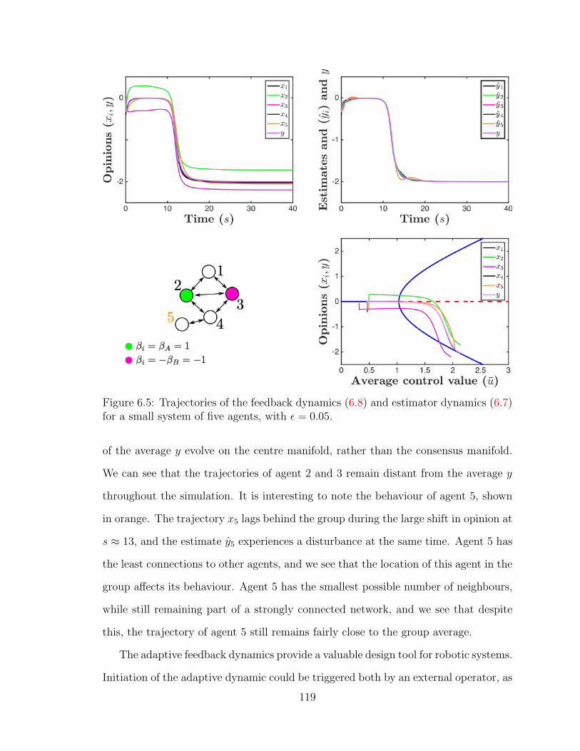
Figure 6.5: Trajectories of the feedback dynamics (6.8) and estimator dynamics (6.7)for a small system of five agents, with ε = 0.05.
of the average y evolve on the centre manifold, rather than the consensus manifold.
We can see that the trajectories of agent 2 and 3 remain distant from the average y
throughout the simulation. It is interesting to note the behaviour of agent 5, shown
in orange. The trajectory x5 lags behind the group during the large shift in opinion at
s ≈ 13, and the estimate y5 experiences a disturbance at the same time. Agent 5 has
the least connections to other agents, and we see that the location of this agent in the
group affects its behaviour. Agent 5 has the smallest possible number of neighbours,
while still remaining part of a strongly connected network, and we see that despite
this, the trajectory of agent 5 still remains fairly close to the group average.
The adaptive feedback dynamics provide a valuable design tool for robotic systems.
Initiation of the adaptive dynamic could be triggered both by an external operator, as
119

well as in response to measurements of the environment by the agents. Let us return
to our example of a search and rescue task, and discuss how these dynamics could
be applied in this situation. With the adaptive dynamics ‘on’, the agents are in a
state that enforces decision-making quickly, while with the dynamics ‘off’ the agents
have more time to explore and measure the environment. In our introduction to the
search and rescue task we discussed how the agents need to be able to transition
between searching separately, and rescuing together, and turning these dynamics on
and off provide a means for facilitating this transition. Additionally, in the early
stage of a search and rescue response, the operators may want the group of agents
to assemble and fully investigate every possible location to search for survivors, but
as time passes the agents should require more evidence to decide on a location. The
adaptive dynamics can be used to modulate how reactive a system is, and how quickly
they make a decision.
Initiating the adaptive dynamics is a simple way for a human operator to interact
with the system at a high level. With these dynamics we provide a method for humans
to interact with the system that does not overly burden them. If the operator was
required to manually adjust the value of u or the decision threshold, it would require
a knowledge of the system dynamics, and how the choices of parameter values will
affect them. With our adaptive dynamics the operator is simply choosing between
“would I like the robots to make a decision soon?” or “would I prefer them to keep
searching?”. The human operator can switch the system between these two states
easily and with limited interaction. In the next chapter, we use a robotic system to
demonstrate more involved interactions between the operator and the system, as well
as to illustrate the flexibility-stability properties of the dynamics.
120

Chapter 7
Robotic Implementation
7.1 Experimental set-up
In this chapter we present the results of experiments performed with a robotic test
platform to demonstrate the application of the decision-making dynamics (3.4) to
a physical system. The format is very simple, and represents the decision-making
sub-system of a full robotic system. The robots choose between two alternatives A
and B, by driving to the right and left sides respectively of the experiment space.
Their horizontal position in the space represents their opinion xi, with the centre of
the room representing xi = 0, and the far right and left of the space strong opinions
for alternatives A (xi > 0) and B (xi < 0). When the robots have collectively reached
a decision they circle in place at the location they have chosen, which represents the
task that a full robotic system would perform once a decision has been made. The
experimental process is depicted in Figure 7.1.
Information about the environment is represented using a coloured light field. Blue
light represents evidence that supports the selection of alternative A and red light
represents evidence that supports the selection of alternative B. The light intensity
corresponds to the evidence strength. In these experiments the light field is controlled
121

Figure 7.1: Flowchart of the experiment process.
by the operator, i.e., the operator assigns the design parameters, but it can also be
thought of as being set by environmental conditions. The light field is not uniform,
as it is created using six spotlights and the intensity is stronger closer to the centre
of the spotlight; this introduces noise into the system.
The robots used were the two-wheeled TurtleBot2 [47], a robot kit for educa-
tional purposes based on the iClebo Kobuki [54]. Each robot has a platform built
on top that supports a single-board computer and light sensor, and the robots can
122

be identified by the platform colour. The robots are each fitted with a light sensor
and take measurements to compute their value of βi, based on a running average.
In our experiments, the pink robot senses red light and the green robot senses blue
light, while the orange robot is an uninformed agent. The robots are connected in a
communication network, which is shown in Figure 7.2.
Figure 7.2: Communication network for the robots.
To achieve a closed-loop system, we use a Vicon motion-capture system that
measures the position and orientation of each robot. We use the horizontal (xi)
position of each robot to represent their opinion xi in the decision-making dynamics,
and the vertical position and orientation for steering commands. The positions x1, x2
and x3 are sent between robots in the communication network, and this is how they
communicate their opinions with each other. We also use the motion capture data in
post-processing, to create the visualisations shown later in this chapter.
Throughout this thesis we have thought of the bifurcation parameter u as the
social effort of the decision-making agents, and also as a control parameter. Here
we focus on the control parameter perspective and consider u a global parameter
that is set by the operator. In other applications the value of u could be set by a
human interacting with the system, or by the robots in response to environmental
parameters. In the previous chapter we discussed thinking of the adaptive feedback on
u as a switch that can be turned on or off, depending on whether a human operator
wishes to enforce a decision being made. In these experiments we can think of a
slightly more complex interaction between a human and the system, where the value
of u is set by a dial, and we will demonstrate ways in which the human can control
various aspects of the behaviour.
123

For ease of use, the decision-making dynamics (3.4) are run on a central computer,
with only the resulting velocities sent to each robot. However, the dynamics of
each agent are calculated separately, so remain distributed, and the system is still
decentralised.
As shown at the bottom of Figure 7.1, the robots can be in one of two states:
the ‘deliberating’ state and the ‘decision’ state. To define the decision state we use
the decision criteria defined in Chapter 3: the decision state is reached if |yss| > η
where η is some threshold value. To determine yss we use the magnitude of the group
average |y|, as well as the `1 norm of the rate of change of their opinion ||x||1. The
condition below on on ||x||1 ensures that the value of y is a steady-state value. For a
choice of threshold η and constants ξ1, ξ2 and ξ3, the robots are in the decision state
if
i. y − η = 0 and ||x||1 < ξ1; the robots have chosen alternative B
ii. y + η = 0 and ||x||1 < ξ1; the robots have chosen alternative A
iii. |y| < ξ2 and ||x||1 < ξ3; the robots are in deadlock, they have chosen to remain
at y = 0.
Otherwise they are in the deliberating state. When they are in the decision state
their velocities are calculated to give a circling motion, and when they are in the
deliberating state their velocities are calculated to represent their changing opinion
xi(t).
The experiments were designed to demonstrate the performance of the decision-
making dynamics and to highlight how the model (3.4) can provide performance that
is both flexible and stable. We describe the results of the experiments and discuss
the performance of the system below.
124
7.2 Results
Videos of each experiment are linked in the text below. This chapter also includes
screenshots of important video frames. Each screenshot shows the network diagram
and the colour of light sensed by each agent, as well as the values of β being broadcast
by the light field and the control value u set by the operator. Additionally, the data
recorded from the motion capture system was used to plot the trajectory of the
average position of the robots against the control value u. The bifurcation diagram
and phase portrait for the current values of u and β parameters are also shown. The
value of the threshold η is represented on the bifurcation diagrams by a dashed black
line. The information displayed showing the values of β are based on the values set by
the operator, not the measurements made by the robots. Hence, the true bifurcation
diagram will differ slightly from what is shown, but due to the robustness properties
of the decision-making dynamics, the expected performance is still achieved.
7.2.1 Experiment 1: Social effort breaks deadlock
Video found at: https://youtu.be/mLdyPezCwQM
The first experiment demonstrates how the social effort u breaks a deadlock between
equal alternatives, and one of the two alternatives is then chosen at random. The
external information parameters were βA = βB = 0.5, and the value of u was raised
and lowered throughout the experiment. In this experiment, both alternatives have
equal value, so when the robots select one of the alternatives for u > u∗, their choice
is determined by their initial conditions. Figures 7.3-7.6 show key frames of the video
of the experiment, with a description of the events shown in each given below.
i. Figure 7.3 : With βA = βB the bifurcation diagram is a symmetric, supercritical
pitchfork. The value of u = 0.8 < u∗ and thus the robots are circling because
they have chosen to remain at the deadlock equilibrium.
125

Figure 7.3: Experiment 1: First screenshot.
Figure 7.4: Experiment 1: Second screenshot.
126

Figure 7.5: Experiment 1: Third screenshot.
Figure 7.6: Experiment 1: Fourth screenshot.
127
ii. Figure 7.4 : The value of u was quickly increased to u = 2.5 > u∗. The dead-
lock equilibrium has become unstable, and the robots move to the equilibrium
corresponding to alternative A and enter the decision state.
iii. Figure 7.5 : The value of u was quickly decreased to u = 0.8 < u∗. The
equilibria representing a decision for either alternative has become unstable,
and the robots return to circle the stable deadlock equilibrium at y = 0.
iv. Figure 7.6 : The value of u was again increased to u = 2.5 > u∗. This time
the position of the robots when they stopped circling was such that they were
closer to the side of the space representing alternative B, so they chose this
alternative.
Although the information broadcast by the lights represented equal alternatives,
due to the non-uniformity of the light field and sensor error, the values of βi sensed by
the robots were not equal. However, as the value of u was quickly increased to a value
much larger than the bifurcation point, the trajectory was in an area of the bifurcation
diagram that is highly robust to disturbances, so we still saw behaviour that we would
expect in a system exhibiting a symmetric pitchfork. By choosing a high u-value, we
chose to prioritise robustness for this experiment, and as such experienced a lower
level of sensitivity. This is a design choice that could be replicated in other situations
when a high level of robustness is required. With high u values, alternatives that
are of near equal value are treated as equal valued, and only a very strong difference
between alternatives would influence the system. Similar to switching on the adaptive
feedback dynamics from the previous chapter, quickly raising the value of u forces
the agents to make a choice, but unlike the adaptive dynamics quickly raising u does
not maintain sensitivity to the environment, except to highly unequal alternatives.
From a design perspective, this experiment shows how a human can interact with
128
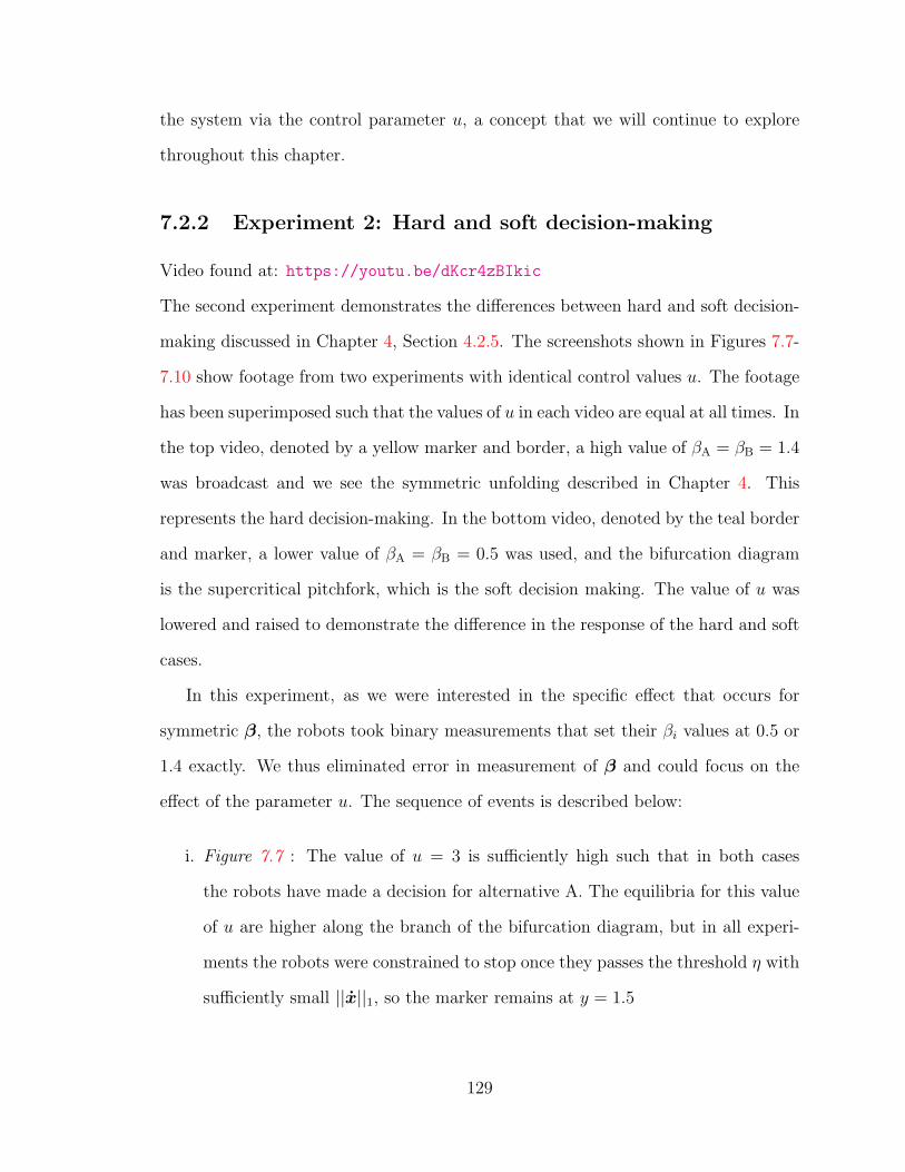
the system via the control parameter u, a concept that we will continue to explore
throughout this chapter.
7.2.2 Experiment 2: Hard and soft decision-making
Video found at: https://youtu.be/dKcr4zBIkic
The second experiment demonstrates the differences between hard and soft decision-
making discussed in Chapter 4, Section 4.2.5. The screenshots shown in Figures 7.7-
7.10 show footage from two experiments with identical control values u. The footage
has been superimposed such that the values of u in each video are equal at all times. In
the top video, denoted by a yellow marker and border, a high value of βA = βB = 1.4
was broadcast and we see the symmetric unfolding described in Chapter 4. This
represents the hard decision-making. In the bottom video, denoted by the teal border
and marker, a lower value of βA = βB = 0.5 was used, and the bifurcation diagram
is the supercritical pitchfork, which is the soft decision making. The value of u was
lowered and raised to demonstrate the difference in the response of the hard and soft
cases.
In this experiment, as we were interested in the specific effect that occurs for
symmetric β, the robots took binary measurements that set their βi values at 0.5 or
1.4 exactly. We thus eliminated error in measurement of β and could focus on the
effect of the parameter u. The sequence of events is described below:
i. Figure 7.7 : The value of u = 3 is sufficiently high such that in both cases
the robots have made a decision for alternative A. The equilibria for this value
of u are higher along the branch of the bifurcation diagram, but in all experi-
ments the robots were constrained to stop once they passes the threshold η with
sufficiently small ||x||1, so the marker remains at y = 1.5
129
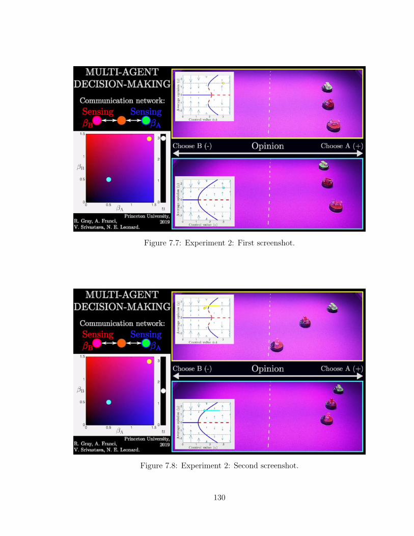
Figure 7.7: Experiment 2: First screenshot.
Figure 7.8: Experiment 2: Second screenshot.
130

Figure 7.9: Experiment 2: Third screenshot.
Figure 7.10: Experiment 2: Fourth screenshot.
131

ii. Figure 7.8 : The value of u was slowly decreased to u = 1.5. In the hard decision-
making (top) case, u < uSN the value of u at the bifurcation of the saddle
node on the upper branch of the diagram, and the robot opinions are attracted
towards to stable branch at y = 0. In the soft decision-making (bottom) case,
the branch of the bifurcation diagram representing a decision for alternative
B remains stable, so the robots stay in the decided state. If u was decreased
further, the trajectory of y would slide down the stable branch towards y = 0,
but would not converge to y = 0 until u < u∗, the bifurcation point of the
supercritical pitchfork.
iii. Figure 7.9 : In the hard decision-making (top) case the robots have converged
to the deadlock equilibrium, which is currently the only stable equilibrium for
this system. In the soft decision-making (bottom) case the robots remain at a
decision for alternative A.
iv. Figure 7.10 : The value of u is slowly increased again back to u = 3. As we
saw in the previous chapter, when u is slowly increased passed the bifurcation
point of a symmetric pitchfork there is some delay before the robots move away
from the now unstable deadlock equilibrium and return to one of the stable
decision branches. In this experiment, the robots returned to choose alternative
A, but either alternative could have been chosen as the bifurcation diagram is
symmetric. Again, in the soft decision-making (bottom) case, the position is
unchanged.
In the hard decision-making case, slowly lowering and then raising u causes hys-
teresis in the trajectory. If the trajectory of the agents is on a branch of the bifurcation
diagram representing a decision for alternatives A or B, when u is lowered past uSN ,
the agents will return to the deadlock solution. The same occurs in reverse if the value
of u is raised again. In the region around the saddle nodes that create the positive
132

and negative branches, the system is highly sensitive to the value of the bifurcation
parameter u, and small changes in u can cause large changes in the average opinion
y.
In the soft decision-making case, slowly lowering u causes the trajectory to slide
down the positive or negative branches. In this case, the change in u was sufficiently
small for the agents to remain at a decision for alternative A for the entire experiment.
If u had been decreased further the trajectory would slide down the positive branch,
and the agents would return to the deliberating state. They would be at a steady-state
value that is less than the threshold, so they would remain in the deliberating state
indefinitely, until the value of u was raised again or lowered below the bifurcation
point.
The symmetric unfolding that leads to hard decision-making occurs for large,
symmetric values of β, and the soft decision-making occurs for small values. Once
the size of a group of agents and the network structure is known, we can determine
that value of β at which the change will occur, and then design gains that multiply
β and determine whether the system is implementing hard or soft decision-making.
When we consider the value of u as a means for human interaction with the system,
adding a tunable gain to β would provide further refinement for how the human
controlling the value of u can affect the system. Alternatively, we can think of u
as being set by a parameter in the environment, or by autonomous dynamics of the
system. The transition from hard to soft decision-making provides a tool to determine
how much changes in the value of u affect the system, or how sensitive the system is
to the value of u.
7.2.3 Experiment 3: Hysteresis due to unfolding
Video found at: https://youtu.be/d12Is2MRrME
In this experiment, we demonstrate the hysteresis that occurs when the value of the
133

two alternatives β is slowly varied, and the shape of the unfolding of the bifurcation
diagram changes. We again show footage from two experiments, with the same values
of β, but with different values of u. The teal markers and border denote the system
with a higher u value, and the yellow markers and border denote the system with a
lower value of u. The yellow system is closer to the bifurcation point, and therefore
more sensitive to the changes in β. Important frames from the video are shown in
Figures 7.11-7.16, and a description of the important events is given below:
i. Figure 7.11 : Initially, βA = 1 and βB = 0, so the bifurcation diagram has
unfolded towards alternative A. For both systems, the value of u is sufficiently
high for them to cross the threshold η, and enter the decision state at alternative
B.
ii. Figure 7.12 : Now βA is slowly lowered from 1 to 0 and βB is slowly raised
from 0 to 1. The shape of the unfolding has changed and for the system at the
lower value of u (yellow/bottom), the equilibrium value of y < η, the decision
threshold, and the trajectory is attracted in the negative direction.
iii. Figure 7.13 : Here, βA < βB, and the direction of the unfolding has changed.
The system with the higher value of u (teal/top) has u > uSN , the value of u at
which the saddle node that creates the positive branch appears, so the robots
in the teal/top remain in the decision state for alternative A.
iv. Figure 7.14 : The trajectory of the (yellow/bottom) system with the lower u
value has now converged to the negative equilibrium branch, and the robots
have made a decision for alternative B
v. Figures 7.15 and 7.16 : As βA is slowly raised from 0 to 1 and βB is slowly
lowered from 1 to 0, we see the same behaviour as Figures 7.13 and 7.14, but
in reverse.
134
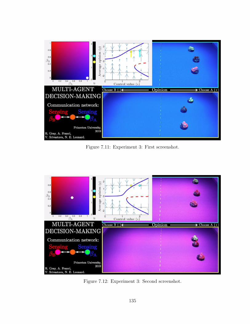
Figure 7.11: Experiment 3: First screenshot.
Figure 7.12: Experiment 3: Second screenshot.
135
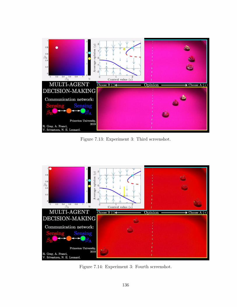
Figure 7.13: Experiment 3: Third screenshot.
Figure 7.14: Experiment 3: Fourth screenshot.
136
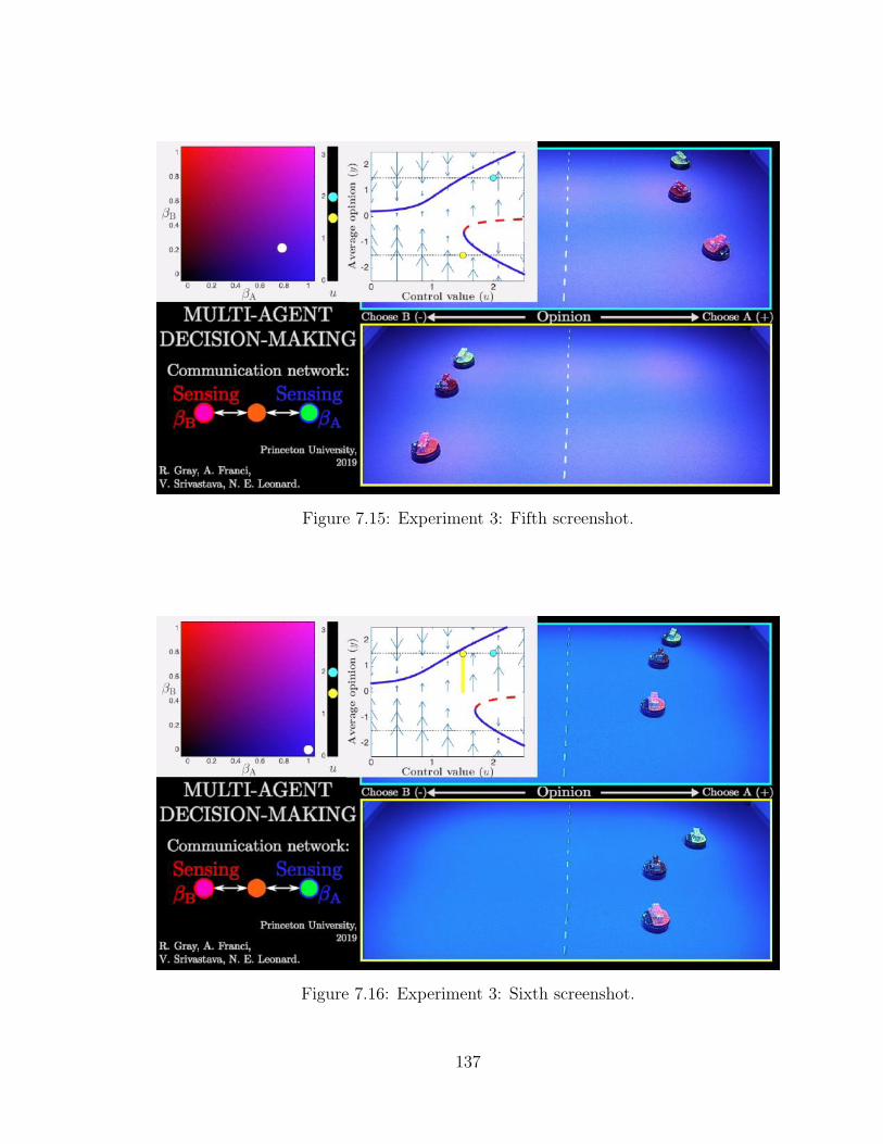
Figure 7.15: Experiment 3: Fifth screenshot.
Figure 7.16: Experiment 3: Sixth screenshot.
137
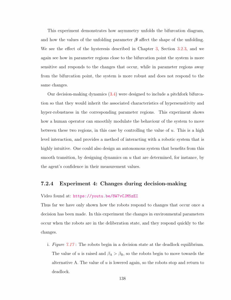
This experiment demonstrates how asymmetry unfolds the bifurcation diagram,
and how the values of the unfolding parameter β affect the shape of the unfolding.
We see the effect of the hysteresis described in Chapter 3, Section 3.2.3, and we
again see how in parameter regions close to the bifurcation point the system is more
sensitive and responds to the changes that occur, while in parameter regions away
from the bifurcation point, the system is more robust and does not respond to the
same changes.
Our decision-making dynamics (3.4) were designed to include a pitchfork bifurca-
tion so that they would inherit the associated characteristics of hypersensitivity and
hyper-robustness in the corresponding parameter regions. This experiment shows
how a human operator can smoothly modulate the behaviour of the system to move
between these two regions, in this case by controlling the value of u. This is a high
level interaction, and provides a method of interacting with a robotic system that is
highly intuitive. One could also design an autonomous system that benefits from this
smooth transition, by designing dynamics on u that are determined, for instance, by
the agent’s confidence in their measurement values.
7.2.4 Experiment 4: Changes during decision-making
Video found at: https://youtu.be/8W7vCJM5zEI
Thus far we have only shown how the robots respond to changes that occur once a
decision has been made. In this experiment the changes in environmental parameters
occur when the robots are in the deliberation state, and they respond quickly to the
changes.
i. Figure 7.17 : The robots begin in a decision state at the deadlock equilibrium.
The value of u is raised and βA > βB, so the robots begin to move towards the
alternative A. The value of u is lowered again, so the robots stop and return to
deadlock.
138
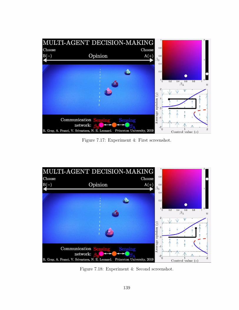
Figure 7.17: Experiment 4: First screenshot.
Figure 7.18: Experiment 4: Second screenshot.
139

Figure 7.19: Experiment 4: Third screenshot.
Figure 7.20: Experiment 4: Fourth screenshot.
140
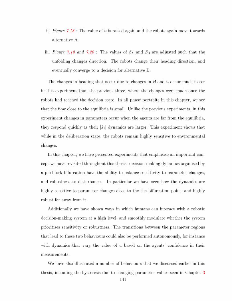
ii. Figure 7.18 : The value of u is raised again and the robots again move towards
alternative A.
iii. Figure 7.19 and 7.20 : The values of βA and βB are adjusted such that the
unfolding changes direction. The robots change their heading direction, and
eventually converge to a decision for alternative B.
The changes in heading that occur due to changes in β and u occur much faster
in this experiment than the previous three, where the changes were made once the
robots had reached the decision state. In all phase portraits in this chapter, we see
that the flow close to the equilibria is small. Unlike the previous experiments, in this
experiment changes in parameters occur when the agents are far from the equilibria,
they respond quickly as their |xi| dynamics are larger. This experiment shows that
while in the deliberation state, the robots remain highly sensitive to environmental
changes.
In this chapter, we have presented experiments that emphasise an important con-
cept we have revisited throughout this thesis: decision-making dynamics organised by
a pitchfork bifurcation have the ability to balance sensitivity to parameter changes,
and robustness to disturbances. In particular we have seen how the dynamics are
highly sensitive to parameter changes close to the the bifurcation point, and highly
robust far away from it.
Additionally we have shown ways in which humans can interact with a robotic
decision-making system at a high level, and smoothly modulate whether the system
prioritises sensitivity or robustness. The transitions between the parameter regions
that lead to these two behaviours could also be performed autonomously, for instance
with dynamics that vary the value of u based on the agents’ confidence in their
measurements.
We have also illustrated a number of behaviours that we discussed earlier in this
thesis, including the hysteresis due to changing parameter values seen in Chapter 3
141

and the transition to the subcritical pitchfork seen in Chapter 4. Also, although we
used a different mechanism to increase the value of u, we saw the same bifurcation
delay that we discussed in Chapter 6, which occurs when the bifurcation parameter
u is slowly varied across the bifurcation point.
142

Chapter 8
Final remarks
In this dissertation, we presented a nonlinear, agent-based model for collective
decision-making between two alternatives. The model was inspired by the dynamics
of a swarm of honeybees selecting a new nest-site. These honeybee dynamics can
be modelled by a pitchfork bifurcation, and by organising our agent-based model
around the same, we can translate mechanisms from the honeybee dynamics to the
agent-based model. The model was derived by Alessio Franci, Vaibhav Srivastava
and Naomi Ehrich Leonard, who also proved, prior to my involvement in the project,
that the agent-based model possesses the pitchfork bifurcation. My contribution to
this project was to analyse and extend the behaviour of the model; to characterise
the behaviour of the model in various parameter regimes, to analyse the influence
of network structure and system parameters on the dynamics, and to demonstrate
ways to augment the model via an adaptive feedback on the social effort parameter,
and interaction with a human operator.
The agent-based dynamics were designed with two aims; to allow us to leverage
mechanisms from the biological settings for application in engineered systems, and
also to ask additional questions about the biological sources of inspiration. In this
thesis we focus on the former aim, and consider how the model and the results of
143

our analysis of the model can be applied to the design of collective decision-making
dynamics for multi-agent systems. We used the example of a network of robotic
agents performing a search and rescue task to consider the results of our analysis in
the context of a real system and also implemented the model with a simple robotic
platform.
We focussed on six design objectives, and discussed how the results of our analysis
improve our abilities to make design choices when implementing our decision-making
dynamics. In Chapter 4 we considered how the system parameters and heterogeneity
affected the dynamics, and showed that, generally speaking, adding heterogeneity to
the system will delay the bifurcation point, and increasing the number of agents in
a group has the opposite effect. We developed a method that reduced the model
to a low-dimensional system for special cases of graphs, which provided additional
tractability for analysis. We used the low-dimensional model to develop a detailed
understand of how the values of the external information about the two alternatives,
the number of uninformed and total number of agents, and heterogeneity in the social
effort parameters affects the decision-making before by changing the location of the
bifurcation point. In the context of a robotic search and rescue task, these results
can be used to inform decisions about the level of social effort u that is required for
the system to make a decision.
In Chapter 5 we showed how the combination of the distribution of external in-
formation and the network structure can lead to a bias in the network even if the
value of the alternatives is equal. This bias is unrepresented by an unfolding of the
symmetric pitchfork bifurcation. We defined two scalar quantities that allow us to
predict the direction of the unfolding for most networks. We then considered the
effects of additive noise, and used analysis of the linearisation of the noisy dynamics
to show that the predictions from the deterministic case could also be applied to the
noisy dynamics. These results are pertinent to our design considerations of the effect
144

of system parameters and the role of the network structure and again, these results
can be applied to making design decisions for decision-making in a robotic network.
Additionally, we showed that the left eigenvector corresponding to the zero eigenvalue
of the network Laplacian is a centrality measure that describes the relative influence
of the nodes in a graph, and can be used to inform decisions about where to place
sensors in a robotic network.
In Chapter 6 we designed decentralised adaptive feedback dynamics that slowly
increase the value of the bifurcation parameter u to ensure that the group will make
a decision. These dynamics addressed the design consideration that the group must
be able to transition from indecision to decision. The slow increase ensures that the
dynamics pass through the region around the bifurcation parameter; an area of high
sensitivity to system parameters.
In Chapter 7 we considered how a human operator can interact with the system, by
performing a series of experiments with a simple network of three agents that choose
which side of the room to drive towards, and received information about the external
environment through sensing a coloured light field. We showed how an operator can
modulate the behaviour of the system through the parameter u. By raising and
lowering the value of u, a human operator can control whether or not a decision is
made, and how sensitive the system is to external parameters. Although this external
control is not necessary for operation of the system, it provides an intuitive means by
which humans can be a part of the decision-making dynamics.
Our final design consideration was the flexibility-stability trade-off; the tension
between designing a system that is sensitive to environmental parameters, but also
robust to disturbances. Throughout this thesis, we saw how the decision-making
dynamics that can be modelled by a pitchfork bifurcation perform successfully in this
trade-off. The dynamics are highly sensitive to environmental and system parameters
in the region close to the bifurcation point, and highly robust far away from it. We
145

can use the value of the bifurcation parameter u to control how close the dynamics
are to the bifurcation point, and therefore how sensitive the system will be at the
given moment. Additionally, through universal unfolding theory we can characterise
all possible behaviours that will occur with perturbations of the dynamics, so there
will be no unexpected behaviour.
8.1 Future directions
A future direction for this work is to return to the other objective identified during the
design of the model; how can we use these dynamics to ask further questions about
the biological sources of inspiration? Previous models for the honeybee dynamics
modelled the decision-making at the population level, and did not allow for consid-
eration of agent heterogeneity or communication network structure. The results of
Chapter 4 prompt questions about the role of heterogeneity in the system; we saw
that an increased level of heterogeneity delayed the bifurcation point, which means
that more social effort is required to break a deadlock and to make a decision. In
our robotic system raising the value of the parameter u was not costly, as it is simply
a parameter in the internally computed dynamics of each agent. We can therefore
easily respond to the level of heterogeneity in a system by changing the value of u. In
the biological setting, raising the level of social effort may be costly. In the honeybee
dynamics the social effort level corresponds to the level of stop-signalling between
bees, and a higher level of social effort requires more activity and energy expenditure.
It may be advantageous for the honeybee dynamics to minimise the amount of het-
erogeneity in the system, so that the decision-making dynamics require less energy
overall.
The results of Chapter 5 show how some agents in a network are more influential
than others, and this can cause a bias in the decision-making dynamics. We used the
146

eigenvector centrality to determine the influence of each node, and this result could
be used to create testable hypotheses for the study of decision-making dynamics in
animal groups. We can model communication networks using proximity or sightlines,
and then use the combination of the simulated networks and eigenvector centrality
to develop an understanding of the role of the communication network for decision-
making in natural systems.
We discussed in Chapter 5 how the external information parameters β entered
the dynamics linearly, and also the Lyapunov-Schmidt reduction. There are two
parameters in the universal unfolding of the symmetric pitchfork, α1 and α2, but with
our model α1 = −βp and α2 = 0. A future project is to adapt the dynamics (3.4)
such that there are analytical relations for both unfolding parameters. This would
allow us to control our location in the parameter region shown in Figure 2.4 (of the
possible unfoldings of the symmetric pitchfork) exactly, and therefore have a higher
level of control over the shape of the bifurcation diagram.
At times in this dissertation we have touched on the speed of decision-making. In
Chapter 4 we discussed the effect of increasing the information value in a system with
S2 symmetry, which led to a sharpening of the pitchfork bifurcation and a transition
from the supercritical pitchfork bifurcation to a subcritical pitchfork bifurcation. If
the value of u was increased at a constant rate, the value of the average opinion y
would increase more quickly for ‘sharper’ bifurcation diagrams. With our current
analysis we can only think about the rate of change of y with respect to the control
parameter u and not time s. Additionally, in Chapter 7 we performed an experiment
which showed that the robots responded to changes in environmental parameters more
quickly when these changes occur while they are in the deliberating state, rather than
the decision state. These observations do not quantify the speed of decision-making
and a extension to this work would be to find bounds on the time until decision, and
to understand the effect of system parameters on the decision-making speed.
147

8.1.1 Current extensions and applications
The transition from the supercritical pitchfork bifurcation to the subcritical pitchfork
bifurcation, and the associated transition from soft to hard-making was considered by
Zhong et al. in [95]. In this work they studied cascade dynamics in a network, and used
the transition between bifurcation diagrams to model when a cascade would or would
not propagate throughout a network. They used similar methods to the analysis
presented here in Chapter 4 to find the parameter values at which the transition
occurs for networks with S2 symmetry.
In this dissertation, we considered a group of N agents choosing between two
alternatives, and in some instances we considered systems with S2 symmetry. An on-
going extension to this work is to consider decision-making between a higher number
of alternatives. In [8], Bizyaeva et al. study decision-making dynamics in systems
with S2 × S2 symmetry; two identical agents choosing between two identical alterna-
tives. The S2 × S2 case is a starting point from which to generalise to higher orders
of symmetry in the number of agents and alternatives, which is the subject of [29].
The ability to decide between a larger number of alternatives would further improve
the applicability of the model to engineered systems.
148

Appendix A
Supporting material for Chapter 3
The following proofs are taken verbatim from [40]. Alessio Franci was the lead con-
tributor to the analysis and writing for these sections, and Vaibhav Srivastava and
Naomi Ehrich Leonard also contributed to and provided guidance for all aspects. An
earlier version of Corollary 2 was presented in [39], provided by Alessio Franci and
Vaibhav Srivastava.
A.1 Proof of Theorem 1
(i) Let V (x) = 12xTx. Then, for 0 < u ≤ 1,
V = x>(−Dx+ uAS(x))
= x>(−Dx+ uDS(x)− uDS(x) + uAS(x))
= −x>D(x− uS(x))− uxTLS(x))
< −ux>LS(x) ≤ 0, ∀x 6= 0,
since uS is a monotone function in the sector [0, 1], D is diagonal and positive definite,
and L is positive semi-definite. Local exponential stability for 0 < u < 1 follows since
149

the linearization of (3.4) at x = 0 is
˙δx = (−D + uA)δx,
and (−D + uA) is a diagonally dominant and Hurwitz matrix.
(ii) Let F (x, u,β) = −Dx + uAS(x) + β, i.e., the right hand side of dynamics
(3.4). Observe that, by odd symmetry of F in x,
F (−x, u,0) = −x = −F (x, u,0).
That is, for β = 0, F commutes with the action of −IN . It follows by [35, Propo-
sition VII.3.3] that the Lyapunov-Schmidt reduction of F at (x, u) = (0, 1) is also
an odd function of its scalar state variable, that is, g(−y, u,0) = −g(y, u,0). To
show that g, and therefore F , possesses a pitchfork bifurcation at the origin for
u = 1, it suffices to show that gyyy(0, 1,0) < 0 and gyu(0, 1,0) > 0. This follows
because all of the degeneracy conditions in the recognition problem of the pitchfork
(gyy(0, 1,0) = gu(0, 1,0) = 0) are automatically satisfied by odd symmetry of g,
and g(0, 1,0) = gy(0, 1,0) = 0 because of the properties of the Lyapunov-Schmidt
reduction [35, Equation I.3.23(a)].
Let v ∈ (Im(L))⊥ be a null left eigenvector of L with |vT1 | =√N , and P =
IN − 1√N
1v> be a projector on Im(L) = 1⊥N . Then, using [35, Equation I.3.23(c)] it
holds that
gyyy(0, 1,0) =⟨v, d3F0,1,0(1,1,1)− 3d2F0,1,0(1, L−1Pd2F0,1,0(1,1))
⟩,
150

where 〈·, ·〉 denotes the inner product, and dkFy,u,β is the k-th order derivative defined
by [35, Equation I.3.16]:
dkFx,u,β(v1, . . . ,vk) =∂
∂t1. . .
∂
∂tkF
(k∑i=1
tivi, u,β
)∣∣∣∣t1=...=tk=0
.
Note that d2F0,1,0 = 0N×N×N because S ′′(0) = 0. On the other hand
∂3
∂xlxkxhFi(x, u,0) = uδkl δ
hkδ
jhaijS
′′′(xj),
which implies that d3F0,1,0(1,1,1)i = uS ′′′(0)∑N
j=1 aij < 0. Since v is a non-negative
vector and not all entries are zero, it follows that gyyy(0, 1,0) < 0.
Similarly, using [35, Equation I.3.23(d)], we have
guy(0, 1,0) =
⟨v, d
∂F0,1,0
∂u(1)
⟩=
⟨v,
[N∑j=1
aij
]Ni=1
⟩> 0,
where we have already neglected the second-order term depending on d2F0,1,0, which
is zero.
It follows by the recognition problem for the pitchfork [35, Proposition II.9.2] that
(3.4) undergoes a pitchfork bifurcation at the origin when u = 1. For u > 1 and |u−1|
sufficiently small, there are exactly three fixed points. The origin is a saddle with an
(N − 1)-dimensional stable manifold corresponding to the N − 1 negative eigenvalues
of −L at the bifurcation and a one-dimensional unstable manifold corresponding to
the bifurcating eigenvalue. The other two fixed point are both locally exponentially
stable because they share the same N − 1 negative eigenvalues as the origin and the
bifurcating eigenvalue is also negative by [35, Theorem I.4.1]. Noticing that (3.4) is a
positive monotone system and that all trajectories are bounded for |u−1| sufficiently
small, it follows from [44, Theorem 0.1] that almost all trajectories converge to the
two stable equilibria, the stable manifold of the saddle separating the two basins of
151

attractions. The location of the three equilibria follows by direct substitution in the
dynamic equations.
(iii) The first part of statement is just the definition of an N -parameter unfolding.
The second part follows directly by [35, Equation I.3.23(d)] �
A.2 Proof of Corollary 2
To prove (i) consider a Lyapunov function Vij(x) =(xi−xj)2
2. It follows that
Vij(x) = −(N − 1)(xi − xj)(xi − xj + u(S(xi)− S(xj)))
< −(N − 1)(xi − xj)2 = −2(N − 1)Vij,
for all xi 6= xj. Therefore, for V (x) =∑n
i=1
∑nj=1 Vij(x), V (x) < −2(N−1)V (x), for
all x 6= ζ1N , ζ ∈ R. V (x) = 0 for xi = xj = ζ, so by LaSalle’s invariance principle,
the consensus manifold is globally exponentially stable.
Using (i), it suffices to study dynamics (3.5) on the consensus manifold, where
they reduce to the scalar dynamics
y = −(N − 1)y + u(N − 1)S(y).
(ii) and (iii) follow by inspection of these scalar dynamics and properties of S. �
A.3 Proof of Theorem 3
Let F (x, u, u,0) denote the right hand side of (3.6) for β = 0. Observe that
F (0, u, u,0) ≡ 0. We show that there exists a smooth function u∗(u) with u∗(0) = 1
such that the Jacobian J(u, u) = ∂F∂x
(0, u, u,0) is singular for u = u∗(u) and suffi-
ciently small u. Moreover, there exist no other singular points close to (0, u∗(u), u).
152

To show this, we apply the implicit function theorem [35, Appendix 1] to the scalar
equation
det (J(u, u)) = 0.
Using Jacobi’s formula for the derivative of the determinant of a matrix, we obtain
∂
∂udet J(u, u) = tr
(adj(J)
∂J
∂u
),
where adj(J) is the adjugate matrix of J [87]. Because Jadj(J) = adj(J)J = det(J)IN
and det(J(1,0)) = detL = 0, it follows that at (u, u) = (1,0) the image of adj(J)
is the kernel of J and that the image of J is in the kernel of adj(J). Recalling that
rank adj(J) = N − rank J = 1, it follows that adj(J(1,0)) = c1NvT0 , where vT0 is a
left null eigenvector of L and c 6= 0. Now, at (u, u) = (1,0),
∂J
∂u= A.
A is non-negative and, by the strong connectivity assumption, at least one element
in each of its columns is different from zero. Furthermore, adj(J)∂J∂u
= c1NvT0A,
and it follows that tr(adj(J)∂J∂u
) = cvT0A1N , which is non-zero. Consequently,
∂∂u
det J(u, u) 6= 0. The existence of the smooth function u∗(β) with the properties
of the statement now follows directly from the implicit function theorem.
Using continuity arguments and the odd symmetry of (3.6), the rest of the theorem
statement follows by Theorem 1. �
153

Bibliography
[1] E. Abed and J. Fu. Local feedback stabilisation and bifurcation control, i. Hopfbifurcation. Systems & Control Letters, 7:11–17, 1986.
[2] E. Abed and J. Fu. Local feedback stabilisation and bifurcation control, ii.stationary bifurcation. Systems & Control Letters, 8:467–473, 1987.
[3] Z. Aminzare, B. Dey, E. N. Davison, and N. E. Leonard. Cluster synchronizationof diffusively coupled nonlinear systems: A contraction-based approach. Journalof Nonlinear Science, pages 1–23, 2018.
[4] P. Antsaklis and J. Baillieul. Guest editorial special issue on networked controlsystems. IEEE Transactions on Automatic Control, 49(9):1421–1423, 2004.
[5] R. Aragues, G. Shi, D. V. Dimarogonas, C. Sagues, K. H. Johansson, andY. Mezouar. Distributed algebraic connectivity estimation for undirected graphswith upper and lower bounds. Automatica, 50(12):3253–3259, 2014.
[6] J. Baillieul and P. J. Antsaklis. Control and communication challenges in net-worked real-time systems. Proceedings of the IEEE, 95(1):9–28, 2007.
[7] N. Berglund and B. Gentz. Noise-induced phenomena in slow-fast dynamicalsystems: a sample-paths approach. Springer Science & Business Media, 2006.
[8] A. Bizyaeva, A. Franci, and N. E. Leonard. Flexible allocation dynamics for twoagents and two options. In preparation, 2019.
[9] J. M. Black. Preflight signalling in swans: a mechanism for group cohesion andflock formation. Ethology, 79(2):143–157, 1988.
[10] R. Bogacz, E. Brown, J. Moehlis, P. Holmes, and J. D. Cohen. The physics ofoptimal decision making: A formal analysis of performance in two-alternativeforced choice tasks. Psychological Review, 113(4):700–765, 2006.
[11] P. Bonacich. Factoring and weighting approaches to status scores and cliqueidentification. Journal of Mathematical Sociology, 2(1):113–120, 1972.
[12] P. Bonacich. Some unique properties of eigenvector centrality. Social Networks,29(4):555–564, 2007.
154

[13] E. Brown, J. Gao, P. Holmes, R. Bogacz, M. Gilzenrat, and J. D. Cohen. Simpleneural networks that optimize decisions. International Journal of Bifurcationand Chaos, 15(3):803–826, 2005.
[14] F. Bullo, J. Cortes, and S. Martinez. Distributed control of robotic networks: amathematical approach to motion coordination algorithms, volume 27. PrincetonUniversity Press, 2009.
[15] J. R. Busemeyer and J. T. Townsend. Decision field theory: a dynamic-cognitiveapproach to decision making in an uncertain environment. Psychological Review,100(3), 1993.
[16] J. Casper and R. R. Murphy. Human-robot interactions during the robot-assistedurban search and rescue response at the world trade center. IEEE Transactionson Systems, Man, and Cybernetics, Part B (Cybernetics), 33(3):367–385, 2003.
[17] I. D. Couzin, C. C. Ioannou, G. Demirel, T. Gross, C. J. Torney, A. Hartnett,L. Conradt, S. A. Levin, and N. E. Leonard. Uninformed individuals promotedemocratic consensus in animal groups. Science, 334(6062):1578–1580, 2011.
[18] I. D. Couzin, J. Krause, N. R. Franks, and S. A. Levin. Effective leadershipand decision-making in animal groups on the move. Nature, 433(7025):513–516,2005.
[19] J. Dethier, G. Drion, A. Franci, and R. Sepulchre. A positive feedback at thecellular level promotes robustness and modulation at the circuit level. Journalof Neurophysiology, 114(4):2472–2484, 2015.
[20] G. Drion, J. Dethier, A. Franci, and R. Sepulchre. Switchable slow cellular con-ductances determine robustness and tunability of network states. PLoS Compu-tational Biology, 14(4):e1006125, 2018.
[21] C. Eikenaar, T. Klinner, L. Szostek, and F. Bairlein. Migratory restlessness incaptive individuals predicts actual departure in the wild. Biology Letters, 10(4),2014.
[22] N. Fenichel. Geometric singular perturbation theory for ordinary differentialequations. Journal of Differential Equations, 1979.
[23] M. Fiedler. Algebraic connectivity of graphs. Czechoslovak mathematical journal,23(2):298–305, 1973.
[24] E. Fiorelli, N. E. Leonard, P. Bhatta, D. A. Paley, R. Bachmayer, and D. M.Fratantoni. Multi-auv control and adaptive sampling in Monterey Bay. IEEEjournal of oceanic engineering, 31(4):935–948, 2006.
[25] K. Fitch and N. Leonard. Joint centrality distinguishes optimal leaders in noisynetworks. IEEE Transactions on Control of Network Systems, 3(4):366–378,2016.
155

[26] A. Fontan and C. Altafini. Multiequilibria analysis for a class of collectivedecision-making networked systems. IEEE Transactions on Control of NetworkSystems, 5(4):1931–1940, 2018.
[27] A. Franchi, C. Secchi, M. Ryll, H. H. Bulthoff, and P. R. Giordano. Sharedcontrol: Balancing autonomy and human assistance with a group of quadrotoruavs. IEEE Robotics & Automation Magazine, 19(3):57–68, 2012.
[28] A. Franci, G. Drion, and R. Sepulchre. Robust and tunable bursting requiresslow positive feedback. Journal of Neurophysiology, 119(3):1222–1234, 2017.
[29] A. Franci, M. Golubitsky, and N. E. Leonard. Flexibility and stability of multi-agent multi-option decision making: A nonlinear dynamics perspective. In prepa-ration, 2019.
[30] A. Franci and R. Sepulchre. Realization of nonlinear behaviors from organizingcenters. In IEEE Conference on Decision and Control, pages 56–61, Los Angeles,CA, Dec. 2014.
[31] A. Franci, V. Srivastava, and N. E. Leonard. A realization theory for bio-inspiredcollective decision making. https://arxiv.org/abs/1503.08526, Mar. 2015.
[32] L. C. Freeman. Centrality in social networks: I. conceptual clarification. SocialNetworks, 1(3), 1979.
[33] K. v. Frisch. Bees-Their Vision, Chemical, Senses And Language. Cornell Uni-versity Press; New York, 1950.
[34] J. George, R. A. Freeman, and K. M. Lynch. Robust dynamic average consensusalgorithm for signals with bounded derivatives. In American Control Conference,2017.
[35] M. Golubitsky and D. G. Schaeffer. Singularities and Groups in BifurcationTheory, volume 51 of Applied Mathematical Sciences. Springer-Verlag, New York,NY, 1985.
[36] M. Golubitsky and I. Stewart. The symmetry perspective: from equilibrium tochaos in phase space and physical space, volume 200. Springer Science & BusinessMedia, 2003.
[37] M. A. Goodrich, A. C. Schultz, et al. Human–robot interaction: a survey. Foun-dations and Trends R© in Human–Computer Interaction, 1(3):203–275, 2008.
[38] W. Govaerts and Y. A. Kuznetsov. Matcont and cl matcont: Continuationtoolboxes in matlab. https://sourceforge.net/projects/matcont/, August 2015.
[39] R. Gray, A. Franci, V. Srivastava, and N. E. Leonard. An agent-based frame-work for bio-inspired, value-sensitive decision-making. IFAC-PapersOnLine,50(1):8238–8243, 2017.
156
[40] R. Gray, A. Franci, V. Srivastava, and N. E. Leonard. Multiagent decision-making dynamics inspired by honeybees. IEEE Transactions on Control of Net-work Systems, 5(2):793–806, 2018.
[41] J. Guckenheimer and P. Holmes. Nonlinear oscillations, dynamical systems andbifurcations of vector fields. J. Appl. Mech, 51(4):947, 1984.
[42] J. Guckenheimer and P. Holmes. Nonlinear Oscillations, Dynamical Systems,and Bifurcations of Vector Fields, volume 42 of Applied Mathematical Sciences.Springer, New-York, 7th edition, 2002.
[43] Y. Hatano, A. K. Das, and M. Mesbahi. Agreement in presence of noise: pseu-dogradients on random geometric networks. In Proceedings of the 44th IEEEConference on Decision and Control, pages 6382–6387. IEEE, 2005.
[44] M. W. Hirsch. Stability and convergence in strongly monotone dynamical sys-tems. Journal fur die reine und angewandte Mathematik, 383(1):53, 1988.
[45] J. J. Hopfield. Neural networks and physical systems with emergent collec-tive computational abilities. Proceedings of the National Academy of Sciences,79(8):2554–2558, 1982.
[46] J. J. Hopfield. Neurons with graded response have collective computationalproperties like those of two-state neurons. Proceedings of the National Academyof Sciences, 81(10):3088–3092, 1984.
[47] O. S. R. F. Inc. Turtlebot2. https://www.turtlebot.com/turtlebot2/, 2019.
[48] S. Inglessis. The flight of the honeybees: Using a multi-agent distributed controlmodel to investigate visual data display. Princeton University Senior Thesis;http://arks.princeton.edu/ark:/88435/dsp01m039k7661, 2018.
[49] A. Jacoff, E. Messina, and J. Evans. A standard test course for urban searchand rescue robots. NIST Special Publication (SP), pages 253–259, 2001.
[50] A. Jadbabaie, J. Lin, and A. S. Morse. Coordination of groups of mobile au-tonomous agents using nearest neighbor rules. Departmental Papers (ESE),page 29, 2003.
[51] J. S. Jennings, G. Whelan, and W. F. Evans. Cooperative search and rescuewith a team of mobile robots. In 1997 8th International Conference on AdvancedRobotics. Proceedings. ICAR’97, pages 193–200. IEEE, 1997.
[52] C. K. Jones. Geometric singular perturbation theory. In Dynamical Systems,pages 44–118. Springer, 1995.
[53] H. K. Khalil. Nonlinear systems. Prentice Hall, third edition, 2002.
[54] Kobuki. About. http://kobuki.yujinrobot.com/about2/.
157
[55] P. Landgren, V. Srivastava, and N. E. Leonard. On distributed cooperativedecision-making in multiarmed bandits. In 2016 European Control Conference(ECC), pages 243–248. IEEE, 2016.
[56] N. Leonard, D. A. Paley, R. E. Davis, D. Fratantoni, F. Lekien, and F. Zhang.Coordinated control of an underwater glider fleet in an adaptive ocean samplingfield experiment in Monterey Bay. Journal of Field Robotics, 27(6):718–740,2010.
[57] N. Leonard, D. A. Paley, F. Lekien, R. Sepulchre, D. Fratantoni, and R. E.Davis. Collective motion, sensor networks, and ocean sampling. Proceedings ofthe IEEE, 95(1), 2007.
[58] N. E. Leonard. Multi-agent system dynamics: Bifurcation and behavior of animalgroups. IFAC Annual Reviews in Control, 38(2):171–183, 2014.
[59] N. E. Leonard and A. Olshevsky. Cooperative learning in multiagent systemsfrom intermittent measurements. SIAM Journal on Control and Optimization,53(1):1–29, 2015.
[60] N. E. Leonard, T. Shen, B. Nabet, L. Scardovi, I. D. Couzin, and S. A. Levin.Decision versus compromise for animal groups in motion. Proceedings of theNational Academy of Sciences, 109(1):227–232, 2012.
[61] W. Li, D. Sadigh, S. S. Sastry, and S. A. Seshia. Synthesis for human-in-the-loopcontrol systems. In International Conference on Tools and Algorithms for theConstruction and Analysis of Systems, pages 470–484. Springer, 2014.
[62] M. Lindauer. Communication among social bees. Harvard University Press, 1971.
[63] E. Marder, T. O’Leary, and S. Shruti. Neuromodulation of circuits with variableparameters: single neurons and small circuits reveal principles of state-dependentand robust neuromodulation. Annual Review of Neuroscience, 37:329–346, 2014.
[64] M. Mesbahi and M. Egerstedt. Graph theoretic methods in multiagent networks,volume 33. Princeton University Press, 2010.
[65] I. R. Nourbakhsh, K. Sycara, M. Koes, M. Yong, M. Lewis, and S. Burion.Human-robot teaming for search and rescue. IEEE Pervasive Computing,4(1):72–79, 2005.
[66] R. Olfati-Saber, J. A. Fax, and R. M. Murray. Consensus and cooperation innetworked multi-agent systems. Proceedings of the IEEE, 95(1):215–233, 2007.
[67] R. Olfati-Saber and R. M. Murray. Consensus problems in networks of agentswith switching topology and time-delays. IEEE Transactions on automatic con-trol, 49(9):1520–1533, 2004.
158

[68] M. Orsag, T. Haus, D. Tolic, A. Ivanovic, M. Car, I. Palunko, and S. Bogdan.Human-in-the-loop control of multi-agent aerial systems. In 2016 European Con-trol Conference (ECC), pages 2139–2145. IEEE, 2016.
[69] D. Pais, P. M. Hogan, T. Schlegel, N. R. Franks, N. E. Leonard, and J. A. R. Mar-shall. A mechanism for value-sensitive decision-making. PloS ONE, 8(9):e73216,2013.
[70] J. K. Parrish and L. Edelstein-Keshet. Complexity, pattern, and evolutionarytrade-offs in animal aggregation. Science, 284(5411):99–101, 1999.
[71] I. Poulakakis, L. Scardovi, and N. E. Leonard. Node classification in networksof stochastic evidence accumulators. arXiv preprint arXiv:1210.4235, 20.
[72] I. Poulakakis, G. F. Young, L. Scardovi, and N. E. Leonard. Information central-ity and ordering of nodes for accuracy in noisy decision-making networks. IEEETransactions on Automatic Control, in press, 2016.
[73] S. R. Ramp, R. E. Davis, N. E. Leonard, I. Shulman, Y. Chao, A. Robinson,J. Marsden, P. Lermusiaux, D. Fratantoni, J. D. Paduan, et al. Preparing topredict: the second autonomous ocean sampling network (aosn-ii) experiment inthe Monterey Bay. Deep Sea Research Part II: Topical Studies in Oceanography,56(3-5):68–86, 2009.
[74] R. Ratcliff. A theory of memory retrieval. Psychological Review, 85(2):59, 1978.
[75] R. Ratcliff and G. McKoon. The diffusion decision model: theory and data fortwo-choice decision tasks. Neural Computation, 20(4):873–922, 2008.
[76] W. Ren and R. W. Beard. Consensus seeking in multiagent systems under dy-namically changing interaction topologies. IEEE Transactions on automatic con-trol, 50(5):655–661, 2005.
[77] W. Ren, R. W. Beard, and E. M. Atkins. A survey of consensus problems inmulti-agent coordination. In Proceedings of the 2005, American Control Confer-ence, 2005., pages 1859–1864. IEEE, 2005.
[78] T. D. Seeley. Consensus building during nest-site selection in honey bee swarms:the expiration of dissent. Behavioral Ecology and Sociobiology, 53(6):417–424,2003.
[79] T. D. Seeley. Honeybee democracy. Princeton University Press, 2010.
[80] T. D. Seeley and S. C. Buhrman. Nest-site selection in honey bees: how welldo swarms implement the “best-of-N” decision rule? Behavioral Ecology andSociobiology, 49:416–427, 2001.
[81] T. D. Seeley, P. K. Visscher, T. Schlegel, P. M. Hogan, N. R. Franks, and J. A. R.Marshall. Stop signals provide cross inhibition in collective decision-making byhoneybee swarms. Science, 335(6064):108–111, 2012.
159
[82] T. Simon, B. Adini, M. El-Hadid, A. Goldberg, and L. Aharonson-Daniel. Therace to save lives: demonstrating the use of social media for search and rescueoperations. PLoS currents, 6, 2014.
[83] V. Srivastava and N. E. Leonard. Collective decision-making in ideal networks:The speed-accuracy trade-off. IEEE Transactions on Control of Network Sys-tems, 1(1):121–132, 2014.
[84] V. Srivastava and N. E. Leonard. On first passage time problems in collectivedecision making with heterogeneous agents. In American Control Conference,pages 2113–2118, Chicago, IL, June 2015.
[85] K. Stephenson and M. Zelen. Rethinking centrality: Methods and examples.Social Networks, 11(1):1–37, 1989.
[86] K. J. Stewart and A. H. Harcourt. Gorillas’ vocalizations during rest periods:signals of impending departure? Behaviour, pages 29–40, 1994.
[87] G. Strang. Linear algebra and its applications. Thomson, Brooks/Cole, Belmont,CA, 2006.
[88] S. H. Strogatz. Nonlinear Dynamics and Chaos: With Applications to Physics,Biology, Chemistry and Engineering. Westview Press, 2000.
[89] D. J. T. Sumpter. Collective Animal Behavior. Princeton University Press, 2010.
[90] H. O. Wang and E. H. Abed. Bifurcation control of a chaotic system. Automatica,31(9):1213–1226, 1995.
[91] S. Wiggins. Introduction to applied nonlinear dynamical systems and chaos.Springer Science & Business Media, 2003.
[92] M. Wooldridge. An introduction to multiagent systems. John Wiley & Sons,2009.
[93] L. Xiao, S. Boyd, and S.-J. Kim. Distributed average consensus with least-mean-square deviation. Journal of Parallel and Distributed Computing, 67(1):33–46,2007.
[94] G. F. Young, L. Scardovi, and N. E. Leonard. Robustness of noisy consensusdynamics with directed communication. In Proceedings of the 2010 AmericanControl Conference, pages 6312–6317. IEEE, 2010.
[95] Y. D. Zhong and N. E. Leonard. A continuous threshold model of cascadedynamics. Submitted to IEEE Conference on Decision and Control, 2019.
160