Designing Bus Bridging Services for RegularEgress

Jiali Du, Shih-Fen Cheng, and Hoong Chuin Lau

School of Information SystemsSingapore Management University

{jiali.du.2012,sfcheng,hclau}@smu.edu.sg

Abstract. We are concerned with the regular egress problem after a ma-jor event at a known location. Without properly design complementarytransport services, such sudden crowd build-ups will overwhelm the ex-isting infrastructure. In this paper, we introduce a novel flow-rate basedmodel to model the dynamic movement of passengers over the trans-portation flow network. Based on this basic model, an integer linearprogramming model is proposed to solve the bus bridging problem per-manently. We validate our model against a real scenario in Singapore,where a newly constructed mega-stadium hosts various large events reg-ularly. The results show that the proposed approach effectively enablesregular egress, and achieves almost 24.1% travel time reduction with anaddition of 40 buses serving 18.7% of the passengers.

Keywords: egress design, bus bridging service,crowd control

1 Introduction

In architectural and urban design community, there is a growing trend to de-sign and build increasingly larger facilities that integrate diverse functions [15].Examples of such facilities include stadiums, convention centers and airports.Operating such facilities with high volumes of human traffic is very challengingand needs to be carefully planned. Issues related to the operation of such fa-cilities include, but not limited to, wayfinding inside the facility, regular egress,and emergency egress. In particular, to serve the transportation needs of crowdsmoving into and out of such facilities, an important consideration is to integratemass transit to the facilities.

In this paper we focus on designing a bus bridging service to complement masstransit during regular egress in order to minimze total journey time of crowds.While regular egress is predictable in both crowd volume and timing (the plannershould know exactly how many people will be leaving the facility, and at whattime), and all utilities can be assumed to be in perfect working condition (whichcontrasts the case of emergency egress, where the timing is uncertain, and someutilities could be faulty), the planning problem is still challenging. The majorchallenge in regular egress is to avoid bottlenecks and crowd buildups, which ishard to avoid since mass transit is designed to satisfy regular transport demands

and not demand surges. A popular solution adopted by many planners is tocomplement mass transit with bus bridging services, yet despite the long historyof using such services, optimizing its delivery has not received much attention;as a result, the design of bus bridging services for regular egress is usually adhoc and static.

In the area of disruption management, however, there are rich literatureon how to optimally utilize bus bridging services to make up for the lost linkor capacity due to disruptions (for instance, in [4], [6], a two-step frameworkfor bus bridging service planning is proposed). Despite the similarity betweendisruption management and regular egress, they are fundamentally different, inthe following aspects. For disruption management, the priority is on restoringas much connectivity as possible, and as a result, the modeling effort has beenmostly on maximizing the amount of flow that can pass through the point ofdisconnection. For regular egress, on the other hand, the focus is on experiencemanagement, which aims at minimizing total journey time including both traveland waiting time. To accurately account for the journey time, we have to modifythe classical flow network so that both travel and waiting times can be quantifiedand thus minimized.

The objective of this paper is to formulate and study the design of busbridging services for regular egress at crowded facilities. In doing so, we makethe following three major contributions:

1. We formulate regular egress as a normalized flow network in which the totaljourney time can be easily calculated.

2. We model the introduction of bus bridging services as an increase to the linkcapacities in the above normalized flow network, and we create an integerprogramming model to derive the optimal design of the bus bridging servicethat would minimize the total journey time for all flows to reach destinations.

3. We demonstrate the practical usage of our model by solving instances in-spired by a real-world scenario. The key parameters of this scenario arederived from a real-world public transport dataset in Singapore.

2 Literature Review

There are extensive works in the literatures discussing about the strategic plan-ning for public transportation services. The general process consists of three ma-jor problems: network design, line planning and timetabling. On solving thesethree major problems, various approaches and techniques were proposed. Net-work design problems focus on altering the configuration of the transportationnetwork for achieving a specific target. This problem was modelled in differ-ent aspects, such as elastic demand [7], directness of both transfer and routes[16]. Due to the high combinatorial complexity of the problem, approximationmethods were proposed in two major streams: heuristics (e.g. [2],[17]) and meta-heuristics (e.g. [9],[11]). Line planning problems mainly discuss the design ofroutes and their relative frequencies over the public transportation network. In[14], Anita et al. proposed an integer programming approach and apply the

Dantzig-Wolfe decomposition method to get the solution. Year after, Ralf et al.presented the branch and price method to solve the problem in [1]. Later in2012, A comprehensive survey of line planning problem was summarized in [13].Timetabling problems refer to the generation of schedules for a set of vehicles ortrains that under specific operational constraints. Various works in the literaturesolve this problem with different objective functions. In [8], Liebchen et al. pro-posed a periodic event-scheduling method to minimize passengers’ waiting timeat transfers by optimizing the Berlin subway timetable. In [5], with the objectiveof minimizing both user inconvenience and operational costs, Kaspi et al. solvethis problem using a cross-entropy metaheuristic method.

Unlike the above works, whose focus were on the strategic planning undernormal situations and improving the service quality during a long term period,our work put the emphasis on minimizing the negative effect caused by the largeevents through establishing the temporary bus links. Reasonable bus planningstrategy in context of the normal cases might not be applicable under the largeevent cases as the passengers demand change dramatically during special hours.Moreover, regular bus service that is suitable for the long term period is un-necessary with respect to the special cases, since the impact results from theevent only last for a few hours. Therefore, we seek strategic planning for thetransportation services under special situations.

One of the special cases is the metro infrastructure disruption managementproblem. Contingency plans were investigated in case of disruption, which canbe found in [3] and [10]. A survey did by Pender et al. on the various practicesto manage the disruption in [12] , which indicated that bus bridging service isthe most common way to minimize the negative impact of the disruption.

In [6], Konstantinos et al. proposed a methodological framework for planningthe bus services. There were two key steps: bus routes planning on the networkand shuttle bus assignment over the selected routes. The optimal bus routeswere generated by using a shortest path algorithm and improved by a heuristicapproach. Following this framework, Jin et al. in [4] formulated the problem byapplying a different approach for generating candidate bus routes compared to[6]. Though the the two-step framework makes the problem tractable to someextent, separation of the two processes, namely candidate routes selection andresources assignment, may cause some inconsistencies. Whereas we optimize theplanning problem in an integrated manner, which covers both processes in oneoptimization model and guarantees optimality for the two simultaneously.

3 Normalized Flow Model for Regular Egress at Facilitieswith Ultra High Demand

3.1 Background

Defined formally, our problem can be represented by a graph incorporating ex-isting public transport service lines, where stations are denoted as nodes andconnectivities denoted as directed links. An example can be seen in Figure 1a,

where there are three lines, each represented by a different line style. Stationsalong all lines are represented as hollow nodes in Figure 1a, the node with ultra-high demand is shaded as node s. Note that node s is not necessarily connectedto existing stations, and visitors at node s might need to find their ways to theclosest station. This might be feasible during normal circumstances, yet whenthe demand is beyond planned capacity, this sudden inflow of demands mightoverwhelm the service provided at the nearby stations.

Line ①

Line ②

Line ③

Source node s

(a) An example of public transporta-tion network with a node emitting ul-tra high demands.

s

d

d d d

l

boundary

ldestinationd rail station transfer station

(b) An example of individual’s trip overthe transportation networks

Fig. 1: Problem description

3.2 Overview

The problem is defined on a graph G = (N , E), where the set N represents allstations, and the set E represents directed links connecting stations. Every linkis defined with a link-specific flow capacity, which will be defined next. In thiscontext, the bus bridging service between two stations is essentially a way toadd capacity to the graph: if the selected two stations are not already connected,a link with corresponding flow capacity will be created; if the selected two sta-tions are already connected, its flow capacity will be increased accordingly. Theplanning horizon is discretized into T time units with equal intervals, whereT is large enough for all travelers to reach their destinations even without anybridging service. The planned bus bridging service can be dynamic, which meansthat it can change over time. The total number of buses that can be deployed isbounded by B.

Let s ∈ N be the source node where surge demands originate. To focus onlyon the part of graph where the bridging service can reach within reasonableamount of time, we define N ⊆ N to be the set containing only nodes thatcan be reached from node s within X minutes (X is empirically set to be large

enough to contain all nodes we will ever consider). Similarly, we define E ⊆ Eto contain all edges between nodes in N . The reduced graph G = (N,E) will beour focus for the rest of the paper. To accurately estimate total journey time, fora passenger who travels to a destination node d not in N , a transfer node l ∈ Nthat’s closest to node d will be chosen as the transfer node, and the remainingtravel time will be accounted for from l to d. In other words, the total journeytime should contain two components: (1) from node s to transfer node l, and (2)from transfer node l to destination d. For travelers whose destination nodes arealready in N , the transfer time will be set to 0. Figure 1b illustrates an exampleof individual’s trip over the transportation networks.

3.3 Normalized Flow Network Model

In classical flow network models (such as the one introduced in [6]), the primaryfocus is on flows, and journey time cannot be derived from the model directly. Toenable the quantification of journey time from flow networks, we introduce timeperiods to the model. To ensure that the model is still tractable after we introducethe time dimension, we make following assumptions. (a). The time period hasequal length; (b). Train arrives with equal frequencies; (c). Travel time on eachlink is equivalent to the train frequency. With these assumptions, we can thensimply recover journey time by summing up flows waiting at all nodes across alltime periods. However, having uniform time periods implies that the travel timebetween any pair of nodes has to be set to the same (single time period) as well.To enable such normalization, for each edge we will calculate the normalizedflow rate to replace capacity, which intuitively refers to the amount of flow thatcan pass through the edge within a single time period. (To understand how thisworks, assume that it takes 5 minutes for a train with the capacity of 100 totravel from a to b, the normalized flow rate for edge (a, b) is then 20 per minute.)

Formally speaking, we define nl,du,t to be the amount of flow waiting at nodeu in time t, with destination node being d and transfer node being l. Similarly,we define xl,du,v,t to be the flow going through the edge (u, v) in time t, withdestination node being d and transfer node being l. The normalized capacity ofthe edge (u, v) in time t is defined as cu,v,t. In other words, for time period t, atmost cu,v,t units of flow can pass from u to v. The normalization procedure willbe described in detail in Section 3.4.

3.4 Deriving Normalized Flow Capacity

As highlighted earlier, total journey time is composed of two major components:the time required to move from s to the transfer node l, which is denoted as δs,l,and the time required to move from l to the final destination d, which is denotedas φl,d. If d ∈ N , φl,d will be set to 0, otherwise it will be pre-computed. δs,l, onthe other hand, will be computed from the normalized flow network as follows:

δs,l =∑

t,u,d,l,u6=l

nl,du,t. (1)

The journey time can be computed as above since flow waiting at any nodesother than the transfer node will require one time period to move forward. Nextwe will explain how we can compute the normalized capacity.

s don board time: Δt

capacity: ϵ t=0t=1t=2

.

.

.t=t

ns=ϵ ns=ϵ-ϵ/Δtns=ϵ-2ϵ/Δt

.

.

.ns=0

nd=0nd=ϵ/Δtnd=2ϵ/Δt

.

.

.ns=ϵ

Fig. 2: An example to illustrate the normalization procedure.

Figure 2 shows an example with two nodes explaining the rationality of thenormalization procedure, where ε is the capacity between the start point s anddestination d and ∆t is the travel time from s to d before normalization.

The purpose of the normalization procedure is to normalize the capacityof the link to be the amount of flow that can pass through in one time unit.The normalized capacity is therefore ε/∆t. After normalization, at the time stept = 1, the total journey time, which consists of wait time and travel time, forthe first ε/∆t unit of flow who successfully pass through the link is (1 + 0) ×ε/∆t = ε/∆t. Similarly, the total journey time for the second ε/∆t unit of flowis (1 + 1)× ε/t = 2ε/t. Generally, the total journey time for the ithε/∆t unit offlow is (i − 1 + 1) × ε/t = iε/∆t. Thus the total journey time for all ε units offlow is

∑ti=1 iε/t = (1 + t)ε/2, which indicates the journey time over the link is

(1+∆t)/2. To correct the bias, we can adding a constant ∆t−(1+∆t)/2 = (∆t−1)/2 to the final average journey time via normalization. As in an optimizationmodel, adding constant to the objective function does not change the solution,therefore, we maintain the calculation of δs,l as formula 1.

Total travel time out of the boundary can be measured according to the num-ber of passengers at transfer node l at the last time step nl,dl,T and the estimatedshortest travel time from l to d: φl,d. Therefore, the total journey time that weseek to minimize will be: ∑

s,l

δs,l +∑l,d

nl,dl,T · φl,d. (2)

Finally, the bus bridging service in our context can be thought of as eithercreating a new edge with capacity αu,v or increasing the existing capacity cu,v,tby αu,v. αu,v is the normalized capacity that corresponds to a particular busservice connecting u and v. The bridging can be time dependent, yet everyassigned bus need to complete its current service before being re-assigned to

serve another route. Our goal is to come up with a bus bridging service thatwould minimize the above total journey time.

4 The Integer Linear Programming (ILP) Model forDynamic Bus Bridging Service During Regular Egress

As highlighted in the previous section, the objective of introducing bus bridgingservice in our paper focuses on reducing total journey time, not making up for thelost capacity (as in the cases of disruption management). The major innovationswe introduce in our mathematical model are: 1) normalization of link capacity toreflect uniform time period length, and 2) the separation of node delay and linkdelay. With these two modeling innovations, we can now formally introduce theinteger linear programming model for optimizing dynamic bus bridging serviceduring regular egress. In our model, the objective is to minimize the total journeytime experienced by all travelers.

min∑s,l

δs,l +∑l,d

nl,dl,T · φl,d.

Let qds,t be the demand size that comes out of node s with destination d in timet. With such dynamic demand, (3) is to ensure the flow conservation for demandnode s, which states that the flow at s in time t is constrained by the flow intime (t − 1) plus the difference between new demands and outgoing flow. Flowconservation for other nodes is described by (4). The next two constraints, (5)and (6), state that outgoing flow of a node u should not exceed the flow at nodeu as well as the capacity of the edge taken.∑

l

nl,ds,t =∑l

nl,ds,t−1 + qds,t −∑l,u

xl,ds,u,t−1 ∀s, t, d, (3)

nl,du,t+1 = nl,du,t +∑w

xl,dw,u,t −∑v

xl,du,v,t ∀u, l, d, t, (4)∑v

xl,du,v,t ≤ nl,du,t ∀u, l, d, t, (5)∑

v

xl,du,v,t ≤ cu,v,t ∀u, l, d, t. (6)

The decision variable ak,ts,u,r is set to 1 if bus k is assigned to link (s, u) in timet. This decision will add additional capacity of αs,u units to edge (s, u), and isexpressed in constraint (7).

cs,u,t = cs,u,0 +∑k,r

ak,ts,u,r · αs,u, ∀s, u, t. (7)

In our formulation, each bus k is allowed to make one intermediate stop beforereaching its destination. In other words, a bus route should contain leg 1 and leg

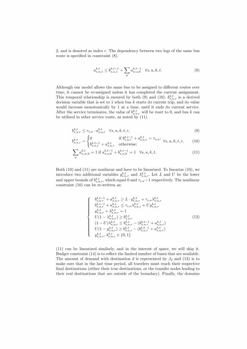
2, and is denoted as index r. The dependency between two legs of the same busroute is specified in constraint (8).

ak,ts,u,1 ≤ bk,t−1s,u,1 +

∑w

ak,t−1w,s,0 ∀s, u, k, t. (8)

Although our model allows the same bus to be assigned to different routes overtime, it cannot be re-assigned unless it has completed the current assignment.This temporal relationship is ensured by both (9) and (10). bk,ts,u,r is a deriveddecision variable that is set to 1 when bus k starts its current trip, and its valuewould increase monotonically by 1 at a time, until it ends its current service.After the service terminates, the value of bk,ts,u,r will be reset to 0, and bus k canbe utilized in other service route, as noted by (11).

bk,ts,u,r ≤ τs,u · ak,ts,u,r ∀s, u, k, t, r, (9)

bk,ts,u,r =

{0 if bk,t−1s,u,r + ak,ts,u,r = τs,u;

bk,t−1s,u,r + ak,ts,u,r otherwise;∀s, u, k, t, r, (10)∑

w

ak,tu,w,0 = 1 if ak,t−1s,u,0 + bk,t−1s,u,0 = 1 ∀s, u, k, t. (11)

Both (10) and (11) are nonlinear and have to be linearized. To linearize (10), weintroduce two additional variables yk,ts,u,r and λk,ts,u,r. Let L and U be the lower

and upper bounds of bk,ts,u,r, which equal 0 and τs,u−1 respectively. The nonlinearconstraint (10) can be re-written as:

bk,t−1s,u,r + ak,ts,u,r ≥ L · yk,ts,u,r + τs,uλk,ts,u,r

bk,t−1s,u,r + ak,ts,u,r ≤ τs,uλk,ts,u,r + Uyk,ts,u,r

yk,ts,u,r + λk,ts,u,r = 1

U(1− λk,ts,u,r) ≥ bk,ts,u,r

(1− U)λk,ts,u,r ≤ bk,ts,u,r − (bk,t−1s,u,r + ak,ts,u,r)

U(1− yk,ts,u,r) ≥ bk,ts,u,r − (bk,t−1s,u,r + ak,ts,u,r)

yk,ts,u,r, λk,ts,u,r ∈ {0, 1}

(12)

(11) can be linearized similarly, and in the interest of space, we will skip it.Budget constraint (14) is to reflect the limited number of buses that are available.The amount of demand with destination d is represented by βd and (13) is tomake sure that in the last time period, all travelers must reach their respectivefinal destinations (either their true destinations, or the transfer nodes leading totheir real destinations that are outside of the boundary). Finally, the domains

of decision variables are listed as the last two constraints.∑l

nl,dl,T = βd ∀d, (13)∑k,s,u,r

ak,ts,u,r ≤ B ∀t, (14)

ak,ts,u,r ∈ {0, 1} ∀s, u, k, t, r, (15)

bk,ts,u,r ∈ {0, τs,u − 1} ∀s, u, k, t, r. (16)

5 Experiment

The effectiveness of our model is demonstrated by a real-world inspired scenarioin Singapore, where a newly constructed multi-purpose national stadium is de-signed to host large events. In this section, we first estimate passengers’ traveldemands based on a real-world public transport dataset. We then perform com-putational experiments to measure the effectiveness of our ILP model. We solvethe ILP model using CPLEX 12.5.

5.1 Dataset Description

The public transport dataset we obtained from our industry partners is calledEZlink1 dataset, which contains each passenger’s boarding and alighting infor-mation (the boarding/alighting stations and times). It contains over one millioncard users’ tap records from 1 Nov 2011 to 31 Jan 2012. We use only recordsfrom work days for consistency.

Inferring Destinations For each card holder h, we maintain a list of candidatedestinations and append the station s′ to the list if: (1) s′ is the first station thath registered as boarding in the morning (before 12 : 00) of a day; or (2) s′ isthe last station that h has registered as alighting during a day after 16 : 00. Theintuition behind this filtering process is based on the assumption that majorityof public transport users would depart from homes in the morning, and leavetheir workplaces in the afternoon. By aggregating records collected over threemonths, we can obtain the frequency of visited stations from the list.

Figure 3 plots an example of the candidate list extracted from 4 card holders.Card holders maintain a set candidate destination stations. It is observed thatmost of the card holders (1,2,3) in the figure have one dominant station s′ whosefrequency is much higher than the rest. This pattern is common when we processthe dataset. We consider a station s′ to be the home location for card holder hif its appearance frequency is over 80%.

If no dominant station can be detected in the list, we will try to clusterstations based on their distance. If the combined frequency of all stations be-longing to the same cluster is high enough, we will consider the home station to

1 http://www.transitlink.com.sg/PSdetail.aspx?ty=catart&Id=1

s1 s2 s3 s4 s5 s6

(a) Card holder 1

s1 s2 s3 s4 s5

(b) Card holder 2

s1 s2 s3 s4 s5 s6

(c) Card holder 3

s1 s2 s3 s4 s5 s6

(d) Card holder 4

Fig. 3: Candidate destination list

be within the cluster. For example, card holder 4 in Figure 3d maintains a listof 6 stations. Although no dominant station can be found, we can identify thecluster of (s1, s2, s3) as they are less than 800 meters from each other. And thecombined frequency for these 3 stations is 90.3%, well above the threshold. Inthis case, we conclude that all of them are close enough to card holder 4’s realhome and thus we use station s1 as the representative home station. If dominanthome station cannot be found for a card hold after the above two checks, we willremove this card from consideration.

In total, we have extracted |D| = 22 important destinations. The distributionof each station s and the travel times from the national stadium s0 to s ∈D are shown in table 1. We treat the set of card users that we identified asrepresentative of the whole city.

Inferring Edge Capacity We obtain the aggregate number of passengers onrail way link (u, v) at time t from the EZLink dataset. The actual flow rate cu,v,ton each link is extracted according to train frequencies. The edge capacity cu,v,tin the model is represented by the additional flow rate, which is defined as thespare space available for passengers and can be inferred from the designed flowrate and actual flow rate .

cu,v,t = dcu,v − acu,v,t. (17)

We assume that the capacity of each bus is 140. In our experiment, the capacityof bus is small compared to the capacity on the links. To reduce the solutionspace (and make the numerical experiments tractable), we assume that we willassign 4 buses at a time.

Table 1: Destination distributions.

station s percentage ∆ts0,s station s percentage ∆ts0,s

Yishun 7.6% 34 Aljunied 4.0% 10Sembawang 7.4% 38 Simei 3.9% 21Admiralty 6.9% 41 Hougang 3.8% 20Yew Tee 6.0% 44 Boon Lay 3.8% 40Ang Mo Kio 5.4% 24 Tiong Bahru 3.8% 16Khatib 4.9% 32 Sengkang 3.7% 24Tampines 4.5% 23 Bukit Batok 3.7% 36Lakeside 4.5% 37 Bukit Gombak 3.7% 38Pioneer 4.3% 42 Woodlands 3.6% 44Choa Chu Kang 4.0% 42 Clementi 3.4% 29Serangoon 4.0% 16 Toa Payoh 3.3% 22

5.2 The Scenario

Let the stadium be the demand originator (s0) with up to 30, 000 people. Timehorizon is assumed to be T = 12 and is enough for all passengers to reach theirrespective destinations. Each time period refers to 6 minutes. In total, there are19 nodes (stations) and 38 links within the boundary.

5.3 Effectiveness

We first discuss the effectiveness of our approach by comparing our ILP model toa rule-of-thumb assignment policy. After consulting industry experts on regularegress from a sports complex, they recommend a rule-of-thumb assignment policyto create a recurrent bus service line running between the sports facility and amajor nearby station (called Cityhall station). Finally, we also assume that theegress for all 30,000 visitors would occur at the same time. Travel time reductionfor both ILP model and rule-of-thumb approach is shown in Figure 4a. Traveltime decreases along the y-axis for both approaches as the number of availablebuses increases along the x-axis. When the number of buses is set to be 0, itshows the very baseline indicating the situation of assigning no bus. On onehand, in terms of the average waiting time reduction, our ILP model improvethe total journey by 15.7 minutes, i.e., a 24.1% reduction, compared to theno bus situation. On the other hand, with a fixed budget, the journey timereduction of our ILP model is larger than the ad hoc method, which indicatesthat the ILP model is more effective in planning the bus bridging services. Forexample, with 40 buses, the ILP model saves almost 4 minutes (8% reduction)for each passenger compared to the rule-of-thumb assignment. This result isnot surprising as the rule-of-thumb assignment only considers the approximatedemand and does not change its strategy over time as need.

Figure 4b depicts the number of passengers that arrives at their target trans-fer nodes over time horizon under 3 different situations. Arriving at the transfer

Num. of buses

Ave

rage

jour

ney

time

(tim

e st

ep)

0 4 8 12 16 20 24 28 32 36 40

7.5

8.0

8.5

9.0

9.510.0

11.0

ILPrule-of-thumb

(a) Average journey time.

time step

Num

. of p

asse

nger

s

0 1 2 3 4 5 6 7 8 9 10 11

05000

15000

25000

No busILPrule-of-thumb

(b) Arrivals to the transfer node.

Fig. 4: Effectiveness.

node is the first step of the whole trip. When there is no bus services incor-porated, passengers gradually approach the target transfer node with a muchslower pace. Before t = 7, when all things being equal, the naive rule-of-thumbapproach serves a increase of around 20% passengers when the planning horizonis going up. This is a stark contrast to our ILP model, in which almost 82% ofpassengers were sent to the transfer node in time t = 4.

One phenomenon observed from Figure 4b is that the ILP approach is notonly effective in sending people to the final destinations but also efficient insending passengers to the transfer node. However, the rate of sending passengerstowards the transfer node after t = 4 decreases significantly. On the other hand,such rate for the rule-of-thumb approach keeps the same even after t = 4.This isbecause the rule-of-thumb strategy requests all of the buses serving on the edgefrom s0 to the preselected station, Cityhall, hence passengers quickly diffuse tothe transfer node. When t = 6, most of the passengers are sent to the transfernode and serving on the route (s0,Cityhall) does not help any more. Rest ofpassengers who did not reach the transfer node would have to rely on regulartrain services and this accounts for the slower movement pace during this t = 6and t = 7.

In our problem, besides the trip within the boundary, another significantfactor that affect the total journey time is the trip from transfer nodes to des-tinations. In addition to the fact that the ILP model can disperse the crowdto the transfer nodes quickly, it also assign passengers to the optimal nodes lfor making transfers. While for the rule-of-thumb approach, it fails to assignpassengers to the optimal transfers which lead to the situation that people maytake longer time to their final destinations.

5.4 Effect of Stop

In this section, we discuss the effect of having alighting stops in our bus bridgingservice. For simplicity, we assume that buses can only start their services fromthe demand node s0 and operate in 2 different ways: 1) creating a direct linkconnecting two stations, and 2) creating a route with one alighting stop. Weassume that all 30, 000 passengers exit the source node simultaneously at timet = 0.

We show the map illustrating the optimal bus routes taken by the above twoservices in Figure 5. In Figure 5a, buses start from the national stadium (labelA with red circle) to a set of stations with label B. In figure 5b, buses start fromthe national stadium and have one alighting stop labeled as B and then at thesame station, start their service towards the end of the service stop.

(a) Direct service (b) One stop service

Fig. 5: Bus routes

Num. of buses

Ave

rage

jour

ney

time

(tim

e st

ep)

0 8 16 24 32 40 48

78

910

11 direct serviceone stop

Fig. 6: Direct service vs one stop service

Figure 6 plots the average journey time experienced by passengers when thenumber of employed buses varies along the x-axis. Intuitively, we observe that forboth services, the average journey time reduces as the number of bus increases.Another observation from Figure 6 is that direct bus service is more effectivecompared to setting an alighting stop under our scenario.

In our ILP model, buses serve for two major roles: (1) facilitate the movementof crowds out of congested area near the demand node s0 (which reduce the traveltime within the boundary); (2) adjust passengers’ trip and accommodate themto the proper transfer node l at lower-density area, which reduce the travel timebeyond the boundary. Easing the congestion near the demand node is the keyfactor that affect passengers’ total journey time. Adjusting the transfer nodefurther improve passengers’ travel experience. As the number of buses is toosmall to handle the demand (48 buses provides services for over 2% passengers),plenty of passengers are clogged near station s0.

6 Conclusion

In this work, we presented a novel normalized flow network approach to modelthe regular egress of a large-scale facility. With such movement model, we proposean ILP-based approach to generate the optimal bus bridging services. The resultsfrom a real-world scenario show that our ILP formulation obtains 24.1% journeytime reduction with only 40 buses providing services for 18.7% of the passengers.Even compared to the rule-of-thumb strategy, where authorities set a bus routebased on experience, it is able to save 8% of the journey time for each passenger.Furthermore, we learn that setting an alighting node along the bus route is nota good choice when the number of available buses is not enough. The futureresearch is to seek more efficient approaches to handle problem instances on alarger scale. In addition, we also look at extending the existing model to provideonline planning strategies.

References

1. Borndorfer, R., Grotschel, M., Pfetsch, M.E.: A column-generation approach toline planning in public transport. Transportation Science 41(1), 123–132 (2007)

2. Chakroborty, P., Wivedi, T.: Optimal route network design for transit systemsusing genetic algorithms. Engineering Optimization 34(1), 83–100 (2002)

3. Janarthanan, N., Schneider, J.B.: Computer-aided design as applied to transit sys-tem emergency contingency planning. Computers, Environment and Urban Sys-tems 9(1), 33–52 (1984)

4. Jin, J.G., Teo, K.M., Odoni, A.R.: Optimizing bus bridging services in response todisruptions of urban transit rail networks. Transportation Science (2015)

5. Kaspi, M., Raviv, T.: Service-oriented line planning and timetabling for passengertrains. Transportation Science 47(3), 295–311 (2013)

6. Kepaptsoglou, K., Karlaftis, M.G.: The bus bridging problem in metro operations:conceptual framework, models and algorithms. Public Transport 1(4), 275–297(2009)

7. Lee, Y.J., Vuchic, V.R.: Transit network design with variable demand. Journal ofTransportation Engineering 131(1), 1–10 (2005)

8. Liebchen, C.: The first optimized railway timetable in practice. TransportationScience 42(4), 420–435 (2008)

9. Mauttone, A., Urquhart, M.E.: A route set construction algorithm for the tran-sit network design problem. Computers & Operations Research 36(8), 2440–2449(2009)

10. Meyer, M.D., Belobaba, P.: Contingency planning for response to urban trans-portation system disruptions. Journal of the American Planning Association 48(4),454–465 (1982)

11. Pattnaik, S., Mohan, S., Tom, V.: Urban bus transit route network design usinggenetic algorithm. Journal of Transportation Engineering 124(4), 368–375 (1998)

12. Pender, B., Currie, G., Delbosc, A., Shiwakoti, N.: Disruption recovery in passengerrailways. Transportation Research Record: Journal of the Transportation ResearchBoard 2353(1), 22–32 (2013)

13. Schobel, A.: Line planning in public transportation: models and methods. ORspectrum 34(3), 491–510 (2012)

14. Schobel, A., Scholl, S.: Line planning with minimal traveling time. In: ATMOS2005-5th Workshop on Algorithmic Methods and Models for Optimization of Rail-ways. Internationales Begegnungs-und Forschungszentrum fur Informatik (IBFI),Schloss Dagstuhl (2006)

15. Tubbs, J., Meacham, B.: Egress design solutions: A guide to evacuation and crowdmanagement planning. John Wiley & Sons (2007)

16. Zhao, F., Ubaka, I.: Transit network optimization-minimizing transfers and opti-mizing route directness. Journal of Public Transportation 7(1), 63–82 (2004)

17. Zhao, F., Zeng, X.: Simulated annealing–genetic algorithm for transit networkoptimization. Journal of Computing in Civil Engineering 20(1), 57–68 (2006)