Design Tradeoffs for Radiation Detection Sensor Networks

Annie Liu, Matt Wu, K. Mani Chandy, Daniel Obenshain, Mason Smith, Ryan McLeanCalifornia Institute of Technology

Pasadena, CA 91125Email: aliu@cs.caltech.edu

ABSTRACTThe detection of hazardous radiation sources is diffi-cult for several reasons. Sensors detect when photons,generated randomly by sources, strike crystals and sosensors don’t get continuous information streams. Ra-diation emanates from threats but also from walls, theground and medical patients undergoing radiation treat-ment. There may be multiple, mobile, evasive sources.The number of parameters is so large that fundamen-tal tradeoffs in designing sensor networks for the prob-lem are unclear. This paper reports on analyses of ba-sic tradeoffs such as mobile versus static sensors; fewlarge sensors versus several small ones; unlimited com-munication range and bandwidth versus limited rangeand bandwidth between sensors. The paper restricts at-tention to detecting sources in a two-dimensional area.Understanding basic tradeoffs - such as the reductionin detection time that accrues from increased speed ofmobile sensors within a 2D field - helps in designingsystems for more complex settings such as urban areaswith buildings and roads.

General TermsAlgorithms, Simulations

KeywordsRadiation detection, wireless sensor network, mobile sen-sors, distributed data processing, detection and tracking

1. INTRODUCTIONIntelligent Personal Radiation Locators (IPRLs) have

been developed recently to detect hazardous radiation

Permission to make digital or hard copies of all or part of this work forpersonal or classroom use is granted without fee provided that copies arenot made or distributed for profit or commercial advantage and that copiesbear this notice and the full citation on the first page. To copy otherwise, torepublish, to post on servers or to redistribute to lists, requires prior specificpermission and/or a fee.Copyright 200X ACM X-XXXXX-XX-X/XX/XX ...$5.00.

sources. These devices have small form factors andare carried by security personnel or on mobile robots.IPRLs communicate with each other and with infor-mation fusion stations through wireless or, in the caseof tethered devices, through wired connections. Intel-ligent radiation sensor systems (IRSS) have been pro-posed to integrate information from multiple detectorsin real time so as to improve the probability of detect-ing hazards, reduce rates of false positives, localize haz-ardous sources more quickly, and differentiate threatsfrom naturally occurring radioactive material (NORM).This paper studies basic tradeoffs in IRSS. Next, someof the fundamental questions that arise in IRSS designsare discussed briefly; details are provided later.

The core of an IPRL is a plate of material that gener-ates current when struck by a photon. Larger plates aremore sensitive because they are more likely to be hit byphotons, but they are also more expensive. What aretradeoffs between fewer, more expensive, more sensitivesensors and greater numbers of less expensive, less sen-sitive sensors? How do these tradeoffs change when sen-sors can or cannot communicate with each other? Whatare good designs for using combinations of stationaryand mobile sensors? Should mobile sensors search spacesindependently and meet periodically to exchange andfuse data, or should they attempt to stay within com-munication range of each other at all times? This pa-per studies such questions using a mathematical modelbased on Bayesian statistics. Parameters of the studyare based on existing and future IPRLs.

Prevention of illicit trafficking of fissionable nucleardevices is a major concern for humanity in general andthe Department of Homeland Security in particular [10].The current solution to the detection of these devices in-volve the use of individual, large, portal-monitor-styledetectors positioned at gate points [11]. Research sug-gests that IRSS are cheaper, more power efficient andenable more rapid deployment than portal monitors [12].Some earlier work suggests diminishing marginal returnsfrom increasing the size of detectors because the signal-to-noise ratio (SNR) does not improve proportionately

to surface area [14]. In this paper we study basic prob-lems, using simple models and easily reproducible ex-periments to gain insight into design tradeoffs.

The major source of error in radiation detection isbackground radiation [5, 14, 11, 6]. Background radia-tion is ionizing radiation emitted from a variety of nat-ural and artificial sources. Primary contributions comefrom the earth’s surface, sky, buildings, and people. Thelevel of background radiation varies with envrionmentalconditions such as rain and snow. Patients who have re-ceived radiological treatment such as Technetium-99 orIodine-131 also emanate photons [12]. More expensivesensors can distinguish harmful radiation sources frombenign sources by their energy spectrum. One of themany tradeoffs to be considered are the relative numberof expensive sensors that identify source signatures ac-curately and the number of less expensive sensors thatdo not.

IRSS are useful in a variety of settings including thedetection of dirty bombers infiltrating political rallieswhile carrying radiation material in backpacks [1]; de-tection of nuclear material on ships by boarding par-ties [2]; and detection of radioactive contraband at air-ports [3]. Models of realistic scenarios, such as detectionby maritime boarding parties carrying sensors, are com-plex; they have to deal with shielding by metal shieldssuch as ship hulls and evasive action likely to be takenby smugglers. We study the simpler problem of detect-ing static sources in a 2-dimensional region so as to gainfundnamental insights into tradeoffs.

We consider the scenario in which radioactive materi-als, such as Cesium-137 or Cobalt-60 are carried into a2-D field and then left in place or are moved slowly bypedestrian terrorists. Sensors have wireless communica-tion capability, as well as GPS or some other locationdetermination mechanism. The system architectures weconsider include combinations of static and handhelddetectors. We study tradeoffs between wireless sensorswith long communication ranges that allow mobile sen-sors to remain in communication contact much of thetime and sensors with short ranges which reduce oppor-tunities for information aggregation.

2. DETECTOR MODELThe traditional Geiger counter is limited by its long

dead time and large size [10]. A collaborative effortbetween Caltech, Smith Technology, and Motorola isbuilding an IPRL based on a Cademinum Zinc Telluride(CdZnTe) detector coupled with GPS, gyroscope, andwirelss capacity.

The CdZnTe detector was introduced only in the lastdecade and has shown great improvement in both sizeand energy resolution over other room temperature op-erated gamma-ray spectrometers, such as NaI scintilla-

tor. The technology with CdZnTe has also made com-pact, light-weight detector systems possible [7] [5]. Theprototype of the IPRL detector consists of a 20mm ×20mm×5mm slab of CdZnTe crystal which is pixelatedinto an aray of 32 × 32 smaller detectors, each withsmaller SNR than a single readout of the full detector.The detector and the platform it is mounted on is light-weight, compact, inexpensive, and potentially suitablefor carrying onto small ground robots and UAVs. Fig-ure 1 shows a model of the IPRL detector

Figure 1: IPRL handheld detector

The current specification of the wireless/GPS moduleis listed below.

Table 1: Wireless Communication Capacity

Parameter Requirement Goal

Location <5m, latitude, longitude <5m(GPS) <50m, altitude

outdoorWireless Range >20m >200m(peer-peer)Wireless Range >300m >5km(peer-master)

3. RADIATION MODEL

3.1 Photon Emission from Radiation SourcePhotons are generated by a radiation source in a Pois-

son manner. Consider a fixed radiation source and afixed detector where the rate at which the detector recordsphotons from the source is λ. Then the probability ofthe detector recording n hits in time interval ∆t givenintensity λ is

P (n | λ,∆t) =(λ∆t)n · e−λ∆t

n!(1)

We approximate a radiation source as a point source.This approximation is reasonable when detectors are farfrom the source. We also assume that photons are sent

with equal intensity in all directions, that is, the sourceis shielded evenly. The detector crystal is approximatedto be a flat plate with surface area A and arbitrarilysmall thickness. These approximations help us gain in-sight into basic tradeoffs such those between many largesensors and few small ones.

Let µ be the rate at which photons are generated bythe source. Let d be the distance between the source andthe detector. The rate at which photons pass througha surface area A on the surface of a sphere of radius dis proportional to A

d2 . The rate λ at which photons aredetected by the sensor is given by:

λ =µ ·A · cos θ

d2(2)

Where θ is the angle between the incoming photon di-rection and the normal to the surface it hits. This equa-tion is only valid when the distance d from the sourceis large. For the parameters of interest, this equationis a satisfactory approximation when d is of the orderof a few meters. In the limiting case, as d approacheszero, λ approaches µ; and we use this correction factorto model the small d case.

Photon Absorption.Equation 2 does not consider absorption of photons by

material on the path between the source and detector.Absorption is calculated as follows. We consider theray from the source to a point on the detector surfaceand determine the material and its density along thatray. We then calculate the probabilty of absorption ofphotons along that ray, and adjust λ accordingly.

Simulating Photon Stream.When the sensor and the source move, the values of

d and θ change with time. In this case λ is time vary-ing and the process by which the sensor detects pho-tons is an inhomogeneous Poisson process. We handlethe time-varying nature of the process by carrying outcalculations in time increments and assuming that thePoisson intensity does not vary within each increment.Using Equation 1, the probability of a detector with in-tensity λ receiving at least one photon hit in time ∆tis:

P (n > 0 | λ,∆t) = 1− e−λ∆t (3)

This equation is accurate provided the time increment∆t is small relative to the linear velocities of the sourceand sensor and the angular velocity of the sensor. Inscenarios such as maritime boarding or patrolling po-litical rallies, IPRLs are carried by security personnel.Changes in orientation when a person turns or looksdown changes θ; We approximate that λ does not change

during the interval when ∆t is small enough. We cannotmake ∆t arbitrarily small, however, because of the deadtime of the sensor. The dead time is the minimum timethat must elapse between consecutive hits in order forthem to register as unique events [5]. The IPRL has adead time of about 2 milliseconds, which is 1

10 of the ∆tused in our simulation. We chose this ∆t to conservethe processing power. This approximation is reasonablebecause in real scnarios, we are likely to be far awayfrom the source and frequent updates are unnecessary.

3.2 Background RadiationContributions from cosmic and atmospheric radiations

do not vary much in a small area and are modeledwith a fixed probability of photon hits at the detec-tor. Contributions of photons from material such asrocks and bricks do vary from detector location to lo-cation. Though our mathematical model accounts forbackground radiation from material, we do not considerthem in the experiments reported in this paper exceptthe very last one because fundamental insights into ba-sic tradeoffs are clouded by consideration of too manyparameters such as location-dependendent backgroundradiation. Therefore, background radiation from ma-terial and cosmic rays is assumed to exist but to beuniform at all points in the area.

4. LOCATION ESTIMATIONWe describe problems in order of increasing realism

and complexity. We begin by considering the problemof detecting a single source and later consider multi-ple sources. We first consider static sources and laterdiscuss moving sources. We begin by assuming thatthe intensity of the source is known and then considerthe more realistic case where source intensity is un-known. In practice, the intensity of a hazardous sourceis unknown because the source may be shielded or theamount of hazardous material is not known. Neverthe-less, simplifying assumptions help us gain insight intobasic tradeoffs.

We use Bayesian methods to calculate the probabil-ity that the source is at each point in the region. Achallenge is to calculate these probabilities quickly. Weassume that each IPRL has computational capability oris connected to a handheld computer. The granularityof calculations can be adjusted to suit available compu-tational power.

The region to be searched is partitioned into incre-mental areas. A simple partitition is an equally-spacedrectangular grid. This approach has the problem of ei-ther too many grid points or grid sizes that are toolarge. Later we consider dynamic gridding where thesizes of grid elements are modified over time so that thetotal number of grid elements is modest and where ar-

eas with parameters changing rapidly over space havesmaller grid elements.

4.1 Single Static Source with Known IntensityIn this scenario we consider the case where a single

source, with known intensity µ, is known to exist some-where in the region. The problem is only to detect wherethe source is. This contrived scenario is useful for ana-lyzing realistic situations.

Consider a uniform grid over the search space. Let thegrid elements be indexed k for k = 1, . . . ,K. Let theprobability that the source is present in a grid elementk at time t be ptk for 1 ≤ k ≤ K, and t = 0, 1, . . .. Sincewe are certain that there is exactly one source in theregion, the sum of probabilities for the region is unity.

∀t :K∑k=1

ptk = 1 (4)

We begin with an a priori distribution of values p0k.

For our experiments we assume a uniform prior distribu-tion over grid elements. For each time step t = 1, 2, . . .,we compute the a posteriori distribution ptk, for all k,given the sensor readings between times t−1 and t, andthe prior distribution pt−1

k for all k. The duration ofeach time step is a constant ∆t.

Consider a scenario with J sensors indexed j = 1, . . . , J ,where J > 0. Let λtj,k be the rate at which photonsfrom a source at grid point k strike sensor j. This ratedepends on the location and orientation of sensor j asspecified in Equation 2. We compute the probabilitythat the source is located at each grid point given thetrajectories of all J sensors. This calculation assumesthat all sensors can communicate with each other or toa base station. Later, we compare these results with thecase where sensor communication bandwidth and rangeare limited.

Let f(ntj |j, k,∆t) be the conditional probability of ntjphotons striking sensor j during the t-th time step giventhat the source is at grid element k. Then, from BayesLaw,

ptkpt−1k

= C

J∏j=1

f(ntj |j, k,∆t) (5)

where C is a constant of proportionality computedfrom Equation 4.

We display pk as gradient of colors on a map, alsoknown as heat map (Figure 2).

We assume that the duration of each time step is smallenough that the probability of two photons striking asensor in a single tick is very small and can be ignored.Thus, during each time step, a sensor detects either no

photons or exactly one photon. Then,

f(n|j, k,∆t) =

{e−λ

tj,k.∆t if n = 0

1− e−λtj,k.∆t if n > 0

(6)

Communication Bandwidth.Consider the bandwidth required for all J sensors to

exchange information. During each update a sensor hasto convey its position (x and y coordinates), orienta-tion (x, y, and z coordinates) and a single bit indicat-ing whether it received a photon or not. The five real-number coordinate values require much more bandwidththan the single bit that indicates the presence or ab-sence of a photon. If, however, the sensors are static orif they are moving along pre-arranged trajectories thencoordinate values of all sensors are known beforehand.

4.2 Unknown IntensityThe Bayesian update method for location estimation

is limited in that it requires knowing all the parametersin Equation 5. In Equation 5, ntj is measured and ∆t isapproximated. However, λj,k is related to the intensityof the source µ, which is often unknown in a real worldsituation (e.g. a dirty bomb threat). A close estimateof source intensity is crucial to estimate the source lo-cation. In this section, we present three methods foracquiring an estimate of source location without know-ing the source intensity.

4.2.1 Parametric Update Using A Priori Distribu-tion of Intensity

We introduce another dimension into the original spaceof uncertainty. The result is a three-dimensional estima-tion problem with the dimensions of consideration being— x, y, µ. We then apply the Bayesian method overthis three dimensional space given an a priori distribu-tion of µ till we reach convergence in both location andintensity. The detailed steps are listed in Appendix A.

4.2.2 Non-Parametric Update in A Sensor GridThe parametric update method is powerful but com-

putationally intensive. Experimental results have alsoshown that the choice of the a priori distribution ofsource intensity is critical to the quality of the pre-dictions. In fact, an ill-posed a priori distribution isworse than no distribution at all. Therefore, the secondmethod for intensity estimation is to neglect µ com-pletely in Equation 5 and update the probability basedonly on the relative distance to the source. More in-formation is included in Appendix B. Though simple toapply, this method does not have the same accuracy asthe other two methods.

4.2.3 Maximum Likelihood Estimator Method

The source intensity and location can be estimated atthe same time using the Maximum Likelihood Estima-tor (MLE) given that we can log the readings from thesensor, GPS, and gyroscope for each detector at eachudpate. The detailed method and derivation are givenin Appendix C.

4.3 Mobile SourceThe position of a source moving along a straight line

can be easily estimated using the Bayesian method withan array of detectors on the side [11]. However, thismethod fails when source movement is random [13]. Wetrack a slow moving source by applying a smoothingbox filter at the ”hot spot” by spreading the probabilityof the most probable location to its neighbors. Ourresult shows that this simple method is robust for speedsup to human running pace. More elaborate methodsuch as Kalman Filter or Particle Filter can be applied.This scenario can be simplified given information of theenvironment that can help predict the movement of thesource [9].

4.4 Multiple SourcesThe conditional probability calculated from Equation 5

assumes the presence of exactly one source in the areaof interest. Multiple sources can thus be identified in aone-at-a-time manner. Our experiments show that sen-sors locate sources near them without too much interfer-ence from distant sensors. After a source is identified,(i.e. when a certain percentage of probability is con-centrated in a small area), it is marked as found at theposition and the conditional probability is recalculatedgiven this information.

4.5 Effect of NoiseThe noise in sensor readings comes mainly from back-

ground radiation. The amount of background radiationcan be coarsely modeled as a uniform increase in de-tector intensity. This information can be collected be-forehand by monitoring the environment with detectorsover a long period of time. If this cannot be done, wecan still estimate the background intensity based on thetypes of objects, such as brick, that are present. Theinfluence from background radiation is considered whencalculating the detector intensity λ using Equation 2.The background noise is generally much weaker thanthe radiation source and does not affect the collabora-tive result of multiple detectors.

Other significant sources are patients who recently re-ceived radiological treatment. In this case, the traceradiation is strong enough to affect the outcome of thedetection (i.e. a false positive). This problem is un-avoidable unless we can examine the spectrum of theraidation. The current solution is to treat it as another

radiation source and rule out its influence after it isidentified using the algorithm descrribed in Section 4.4.

5. DETECTION ALGORITHMSThe Bayesian update method described in Section 4

allows us to partition the field of interest into the moreprobable area and the less probable area. This sectionillustrates three algorithms to efficiently explore theseareas based on the constraints given. We first considerthe simplified case where there is no restriction on wire-less capacity. This discussion serves as a stepping stonewhen we discuss the realistic case where detectors havelimited range and bandwidth.

5.1 Unlimited Range and BandwidthAt each update (∆t = 0.02), all detectors broadcast

messages of new data obtained since the last update.The message consists of the current position of the de-tector, the direction it is facing, and whether it receivesa hit or not in the last ∆t. The packet takes the follow-ing format.

Table 2: Packet Format (20 bytes + 1 bit)

4 bytes 4 bytes 4 bytes 4 bytes 4 bytes 1 bit

xpos ypos xfac yfac zfac 0/1

The detectors udpate their local a posteriori distri-bution based on all the information received. Since alldetectors can communicate with each other, their localmaps should be the synchronous view of the global map.

Algorithm 1.Each detector then moves towards the hottest spot

(area with the highest probability) xhot on its map in-dependently. The trajectory is not a straight line fromits current position to xhot but a spiral that maximizesthe sum of probabilites on its way to xhot. It is sufficientthat the detector stays at a distance of 4 meters awayfrom xhot because little is gained by moving closer. Ifthe source is real, the detector marks the spot as a foundsource and notifies all other sensors in the network.

5.2 Limited Range and BandwidthBased on the specification in Table 2, we assume the

wireless communication is limited by 100 bytes/sec and100 meters for peer-to-peer message exchange. To meetthese constraints, we first reduce the udpate rate fromevery 0.02 seconds to every 0.3 seconds. We can com-pensate for the loss of information between udpates bychanging the packet format to include photon hits sincethe last updates. Other sensor can use this informationto extrapolate the trajectory of a certain detector sincethe last update. The new packet becomes:

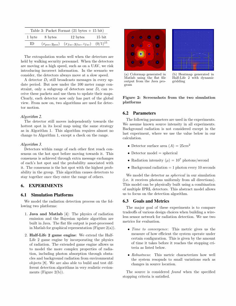
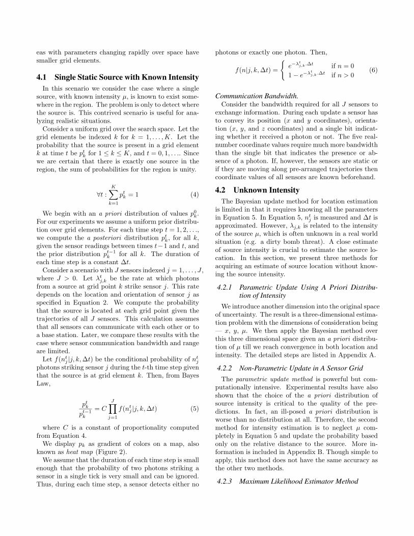
Table 3: Packet Format (21 bytes + 15 bit)

1 byte 8 bytes 12 bytes 15 bit

ID (xpos, ypos) (xfac, yfac, zfac) (0/1)15

The extrapolation works well when the detectors areheld by walking security personnel. When the detectorsare moving at a high speed, such as on a UAV, we riskintroducing incorrect information. In the scenario weconsider, the detectors always move at a slow speed.

A detector Di still broadcasts messages in every up-date period. But now under the 100 meter range con-straint, only a subgroup of detectors near Di can re-ceive these packets and use them to update their maps.Clearly, each detector now only has part of the globalview. From now on, two algorithms are used for detec-tor motion.

Algorithm 2.The detector still moves independently towards the

hottest spot in its local map using the same strategyas in Algorithm 1. This algorithm requires almost nochange to Algorithm 1, except a check on the range.

Algorithm 3.Detectors within range of each other first reach con-

sensus on the hot spot before moving towards it. Thisconsensus is achieved through extra message exchangesof each’s hot spot and the probability associated withit. The consensus is the hot spot with the highest prob-ability in the group. This algorithm causes detectors tostay together once they enter the range of others.

6. EXPERIMENTS

6.1 Simulation PlatformsWe model the radiation detection process on the fol-

lowing two platforms:

1. Java and Matlab [4]: The physics of radiationemission and the Bayesian update algorithm arebuilt in Java. The flat file output is post-processedin Matlab for graphical representation (Figure 2(a)).

2. Half-Life 2 game engine: We extend the Half-Life 2 game engine by incorporating the physicsof radiation. The extended game engine allows usto model the more complex properties of radia-tion, including photon absorption through obsta-cles and background radiation from environmentalobjects [8]. We are also able to build and test dif-ferent detection algorithms in very realistic evrion-ments (Figure 2(b)).

(a) Colormap generated inMatlab using the flat fileoutput from the Java pro-gram

(b) Heatmap generated inHalf-Life 2 with dynamicgridding

Figure 2: Screenshots from the two simulationplatforms

6.2 ParametersThe following parameters are used in the experiments.

We assume known source intensity in all experiments.Background radiation is not considered except in thelast experiment, where we use the value below in ourcalculation.

• Detector surface area (A) = 25cm2

• Detector model = spherical

• Radiation intensity (µ) = 107 photons/second

• Background radiation = 1 photon every 10 seconds

We model the detector as spherical in our simulation(i.e. it receives photons uniformly from all directions).This model can be physically built using a combinationof multiple IPRL detectors. This abstract model allowsus to focus on the detection algorithm.

6.3 Goals and MetricsThe major goal of these experiments is to compare

tradeoffs of various design choices when building a wire-less sensor network for radiation detection. We use twometrics for evaluation.

• Time to convergence: This metric gives us themeasure of how efficient the system operate undercertain configuration. This is given by the amountof time it takes before it reaches the stopping cri-teria as listed below.

• Robustness: This metric characterizes how wellthe system resopnds to small variations such aschanges in source location.

The source is considered found when the specifiedstopping criteria is satisfied.

• Criteria 1 : 50% of the probability is concentratedin 1% of the area of the field.

• Criteria 2 : 95% of the probability is concentratedin 1% of the area of the field.

6.4 Formations of Static DetectorsWe start by asking the question, ”How should we de-

ploy a collection of static detectors?”. In this section, wepresent two types of formations — Line, and Square —and compare the result based on the assumptions thatthe detector can communicate with unlimited range andbandwidth. These experiments provide insight into sit-uations where sensors are arranged randomly with thestraight line and square being extreme cases becausethe square formation is desirable and the straight line ispoor. The results are evaluated using Criteria 1. Eachdata point is the average of 50 independent trials.

6.4.1 LineWe consider a line of nine spherical detectors, each 30

meters apart, on one side of a 300×300 meters field, 30meters from each edge. A radiation source is placed ata distance L perpendicular from the center of the line.

Figure 3 shows that the convergence time increasesexponentially as the source moves away from the lineformation. As expected, the line formation is not robustto variations in source location. However, if we limit thefield size to a narrow area (i.e. a road with detectorslining along a side), then the performance is good.

Figure 3: The convergence time increases expo-nentially as the source moves away from the lineformation.

6.4.2 SquareWe study how the system behaves in a square forma-

tion as we increase the field size and as we change therelative position of the detectors and the source in thefield.

Varying Field Size.

In an empty field of dimension L meters by L meters,we place one detector at each corner and a radiationsource in the center of the field (Figure 5(a)).

As the field size (L2) increases, the convergence timeincreases approximately quadratically (Figure 4). Asexpected, this growth is much better than a line forma-tion.

Figure 4: The convergence time increasesquadratically as the field size increases in asquare formation.

Varying Sensor Positions.In a fixed field of dimension 300×300 meters, we place

four detectors forming a square with sides of length L inthe middle of the field, surrounding a radiation source.While keeping the field size constant, we increase thesize of the square and measure the time it takes to locatethe source (Figure 5(b)). The difference between thisexperiment and the previous one is that the sensors arenot at the corners of the square field.

(a) Varying field size (b) Varying sensor posi-tions

Figure 5: Experiment setups

The convergence time increases as the detector for-mation moves further away from the source as shownin Figure 6. Note a local minimum present at L = 200m. The experiment is repeated for various field size,and this local minimum consistenly appear at L = 2

3S,where S is the side length of the field. This phenomenon

occurs because at this distance, the inverse relationshipbetween detector intensity and distance allows the de-tectors to rapidly rule out the possibility of having asource in the corner.

Figure 6: Convergence time increases as detec-tors move away from the source. Local minimumoccurs at L = 2

3S.

Varying Source Position.We study the optimal position for deploying detectors

in a square formation in a fixed sized field. In a 50× 50meters field, four sensors are locked in a square forma-tion of side length L = [10, 20, 30, 40, 50] centered inthe field. A radiation source is positioned at a distanced = [0, 5, 10, 15, 20] from the center of the field (Fig-ure 7). We measure the convergence time as L increasesand as d increases.

Figure 7: Detectors are placed at the corners of asquare of varying size L with a source at varyingdistance d to the center.

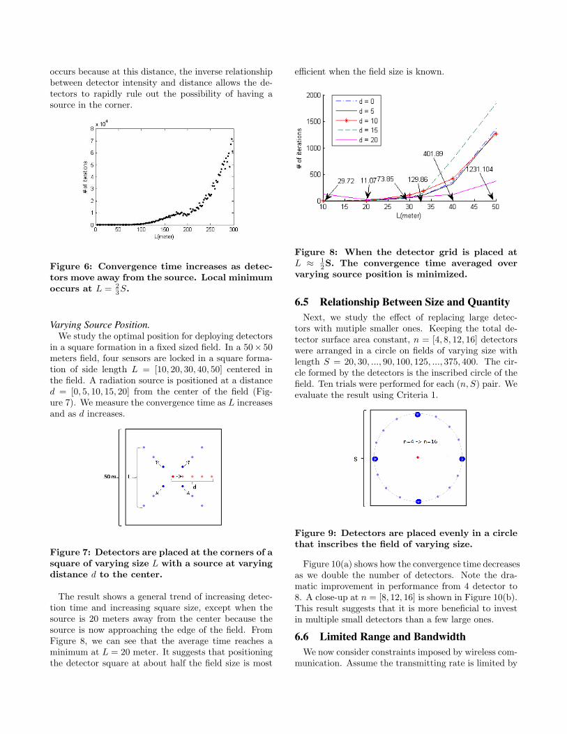
The result shows a general trend of increasing detec-tion time and increasing square size, except when thesource is 20 meters away from the center because thesource is now approaching the edge of the field. FromFigure 8, we can see that the average time reaches aminimum at L = 20 meter. It suggests that positioningthe detector square at about half the field size is most

efficient when the field size is known.

Figure 8: When the detector grid is placed atL ≈ 1

2S. The convergence time averaged overvarying source position is minimized.

6.5 Relationship Between Size and QuantityNext, we study the effect of replacing large detec-

tors with mutiple smaller ones. Keeping the total de-tector surface area constant, n = [4, 8, 12, 16] detectorswere arranged in a circle on fields of varying size withlength S = 20, 30, ..., 90, 100, 125, ..., 375, 400. The cir-cle formed by the detectors is the inscribed circle of thefield. Ten trials were performed for each (n, S) pair. Weevaluate the result using Criteria 1.

Figure 9: Detectors are placed evenly in a circlethat inscribes the field of varying size.

Figure 10(a) shows how the convergence time decreasesas we double the number of detectors. Note the dra-matic improvement in performance from 4 detector to8. A close-up at n = [8, 12, 16] is shown in Figure 10(b).This result suggests that it is more beneficial to investin multiple small detectors than a few large ones.

6.6 Limited Range and BandwidthWe now consider constraints imposed by wireless com-

munication. Assume the transmitting rate is limited by

(a) n=4,8,12,16 (b) n=8,12,16

Figure 10: The convergence time decreases aseach doubling of the detector number while thetotal surface area remains constant. Note theperformance gain has deminishing marginal re-turns.

100 byte/sec and the transmitting range between peersby 100 meters.

6.7 Study of Group SizeOne way to overcome the range limitation is to have

the detectors move in tight formations as stated in Al-gorithm 3. But if so, how big should the group big?Do larger groups always perform better? This exper-iment studies the relationship between group size anddetection efficiency. In a field of 300× 300 meters witha radiation source in the center, n = [4, 8, 16] detectorsare placed on the perimeter of a circle of diameter 100meters at a distance d = [0, 25, 50, 75, 100, 125, 150] me-ters away from the source (Figure 11). Any two detec-tors can communicate with each other in this formation.The result is evaluated using Criteria 1.

Figure 11: A group of n detectors form a cicularformation at a distance d from the source.

Figure 12 shows that as we increase the number ofdetectors in the group, the detection time goes down.However, the incremental improvement decreases as thegroup size gets larger. From n = 4 to n = 8, the amountof time for detecting a source 150 meters away is halved.But from n = 8 to n = 16, it only improves by less than

Figure 12: The convergence time decreases aswe increase the group size. However, the perfor-mance gain has deminishing marginal returns.

13 . In fact, for d > 150 the stopping criteria is not satis-fied for any group size. This result is expected becauseat a distance, a group of tightly formed detectors can beviewed as one large detector. Thus, the result from Sec-tion 6.5 can be generalized to explain this phenonmenon,that is, multiple smaller groups are more effecient thanone large group.

6.8 Gains from SpeedThe performance of a static detector is limited by its

distance to the radiation source. If static detectors areill-positioned and distance to the source is large, detec-tors may not get a single photon hit over a long periodof time, as shown in the previous experiments. Mobiledetectors overcome this problem. But will mobile detec-tors out-perform static ones even under range and band-width constraints? How will the performance changewhen the field size is increased? Will mobility help dealwith noise? This experiment studies the performanceimprovement, if any, from increasing the speed of thedetectors in two different size of fields. We test the sim-ple Detection Algorithm 2 and compare it to the naiveAlgorithm 1 where there is no range or bandwidth lim-itation. The result is evaluated using Criteria 2.

6.8.1 Small FieldIn a field of 300 × 300 meters, 16 detectors are laid

down evenly in a grid formation at time t = 0 (Fig-ure 13(a)). Initially, each detector is 80 meters awayfrom its nearest neighbors, and can thus communicatewith at most 4 detectors, as opposed to 16 when therange and bandwidth are unlimited. The detection timeis measured for detector with speed v = [0, 0.5, . . . , 10]m/s.

The result is shown in Figure 14(a). At speed v = 0m/s (static), detectors with range limitation take 217seconds to determine the location of the radiation source,

(a) Small field (b) Large field

Figure 13: 16 detectors are placed evenly in thefield initially.

whereas detectors with no limitation take only 173 sec-onds. The difference in performance between the twodiminish for v ≥ 1 m/s. For v ≥ 2 m/s, there is almostno gain in performance from increasing the speed in asmall field. This result may be due to the simplicityof Algorithm 2, where the detectors do not collaborateessentially.

6.8.2 Large FieldThe same experiment in 6.8.1 is repeated in a larger

field of 1000 × 1000 meters. Initially, each detector is250 meter away from its nearest neighbors. The resultis shown in Figure 14(b). Note the missing data pointat v = 0. Stationary detectors with range limitationare unable to communicate with anyone else and thusthe source can never be identified. However, once thedetectors start moving, even as slow as 0.5 m/s, thisproblem is resolved. Also note that in a larger field,where detectors are out of range with each other morefrequently than in Section 6.8.1, the detectors with norange limitation consistently perform better by ≈ 150seconds.

6.9 Effect of Background NoiseThe experiment in 6.8.1 is repeated with the presence

of a strong uniform background radiation of detectorintensity of 1 photon hit every 10 seconds. The result isshown in Figure 14(c). Compared to Figure 14(a), thedetection time doubles for each data point for both typeof detectors. However, the shape of the curve remainsthe same, so our findings above are still valid under theinfluence of background noise.

7. CONCLUSIONThis paper evaluates design tradeoffs in designs of in-

telligent radiation sensor systems constructed by fus-ing data from multiple wireless-enabled, static and mo-bile intelligent personal radiation locators. The develop-ment of IRSS from existing and planned IPRLs is impor-tant for the nation’s security. IRSS are ideal examples

(a) Small field

(b) Large field

(c) Small field with background noise

Figure 14: Mobile detectors with communica-tion range and bandwidth limitation

of information processing in sensor networks. Our groupat Caltech has been working with partners on designingand implementing IPRLs; the research reported in thispaper explores basic questions about potential benefitsfrom integrating information from multiple IPRLs. Theanalysis presented here deals with fundamental issuessuch as understanding the decrease in time to locate aradiation source as a function of the number of sensors,speeds of mobile sensors, and tradeoffs of more smallsensors versus few large sensors. Understanding thesebasic canonical problems gives insight that helps in deal-

ing with more complex problems such as the optimumstrategies to be used by maritime boarding parties thathave to deal with the photon-shielding effects of ships’metal structures and evasive action taken by traffickers.

The experiments show that networks of collaboratingIPRLs locate threats much faster than non-collaboratingIPRLs. Thus, our experiments make a strong case forIRSS. The analysis also demonstrates that networks ofmobile sensors are much more effective than networksof stationary sensors. Our analysis shows that there arebenefits to increasing the number of sensors with dimin-ishing marginal returns with the addition of each sensor.Likewise, the time to detect a source decreases with thespeed of mobile sensors, but here too there is diminish-ing marginal returns. An important finding is that bymoving, using the simplest algorithm, at a speed as slowas 0.5 m/s, and under the range and bandwidth con-straints with the presence of background noise, the un-solvable detection problem becomes solvable. This resultstrengthens the idea of replacing large portal style sen-sor with mobile handheld sensor network carried by se-curity personnel. The analysis and programs describedhere can be used to determine configurations of networksof static and mobile sensors most appropriate to givenproblems.

Further work needs to be carried out on realistic sce-narios such as protecting people in stadiums and publicmalls from dirty bombers, and in interdicting nuclearmaterial from ships and at ports and airports. Suitesof experiments should be carried out on evasive actionthat may be taken by people carrying nuclear mate-rial. Gaming environments that help security peopleplay roles of terrorists and first responders will help indealing with evasive action[8]. Finally, IRSS will haveto be tested in the field to evaluate their effectiveness inrealistic situations.

8. REFERENCES[1] Thomas Tisch Devabhaktuni Srikrishna, A.

Narasimha Chari. Deterrence of nuclear terrorismwith mobile radiation detectors. TheNonproliferation Review, 12(3):573–614, 2005.

[2] Shawn P. Gallagher. A system for the detection ofconcealed nuclear weapons and fissile materialaboard cargo cotainerships. Master’s thesis,Massachusetts Institute of Technology. Dept. ofNuclear Engineering, 2005.

[3] Timothy Coffey Gary W. Phillips, David J. Nagel.A primer on the detection of nuclear andradiological weapons. Technical report, Center forTechnology and National Security Policy NationalDefense University, 2005.

[4] Ryan McLean K. Mani Chandy, Concetta Pilotto.Networked sensing systems for detecting people

carrying radioactive material. Fifth InternationalIEEE Conference on Networked Sensing Systems(INSS), June 2008.

[5] Glenn F. Knoll. Radiaiton Detection andMeasurement. John Wiley and Sons Inc., 3rdedition, 2000.

[6] Hai-Feng Ji Thomas Thundat LalA. Pinnaduwage, Member. Moore’s law inhomeland defense: An integrated sensor platformbased on silicon microcantilevers. IEEE SensorsJournal, 5(4), 2005.

[7] William A. Mahoney Larry S. Varnell. Radiationeffects in cdznte gamma-ray detectors producedby 199 mev protons, 1996.

[8] K. Mani Chandy Matt Wu, Annie Liu. Virtualenvironment for developing strategies forinterdicting terrorists carrying dirty bombs. 6thInternational Conference on Information Systemsfor Crisis Response and Management (ISCRAM),2008.

[9] Timothy G. McGee and J. Karl Hedrick.Guaranteed strategies to search for mobile evadersin the plane. Proceedings of the 2006 AmericanControl Conference Minneapolis, Minnesota,USA, 2006.

[10] Brad Millet Chester G. WilsonRandy Waguespack, Scott Pellegrin. Integratedsystem for wireless radiation detection andtracking. IEEE Region 5 Technical Conference,2007.

[11] David C. Torney Tony T. Warnock RobertJ. Nemzek, Jared S. Dreicer. Distributed sensornetworks for detection of mobile radioactivesources. IEEE Transactions on Nuclear Science,51(4), 2004.

[12] David C. Torney Sean M. Brennan, AngelaM. Mielke. Radiation detection with distributedsensor networks. Computer, 37(8):57–59, August2004.

[13] Mukundan SridharanVinodkrishnan Kulathumani, Anish Arora. Trail:A distance sensitive sensor network service fordistributed object tracking. Proceedings ofEuropean Conference on Wireless SensorNetworks (EWSN), 2006.

[14] K.P. Ziock and W.H. Goldstein. The lost source,varying backgrounds and why bigger may not bebetter. In J. I. Trombkar, editor, UnattendedRadiation Sensor Systems for RemoteApplications, pages 60–70. American Institute ofPhysics, New York, 2002.

APPENDIXA. PARAMETRIC UPDATE USING A PRI-

ORI DISTRIBUTION OF SOURCE INTEN-SITY

The modified Bayesian Update method for intensityestimation is as follows. Initially we choose a distri-bution of [µ1, µ2, . . . , µn] with uniform probability thatsums to 1. The range of µi is based on informed guessof the source intensity. Of each µi, we apply Equation 5to get the a posteriori distribution.

ptikpt−1ik

=J∏j=1

f(ntj , λijk,∆t) (7)

The resulting probability distribution map is the nmaps superimposed onto one with ptk being the sum ofall ptik.

ptk =n∑i=1

ptik (8)

After normalizating using Equation 4, we get the finalpk. We can also examine the a posteriori distribution ofµi. The probability of a specific µi being the real sourceintensity is calculated.

P (µi = µ) =∑Kk=1 pik∑Kk=1 pk

(9)

After a few iterations of the above process, the a pos-teriori distribution in intensity and location both con-verge.

B. NON-PARAMETRIC UPDATE METHODWe can define pj(x, y) as the conditional probability

that detector Dj detects a photon emitted by a source atlocation(x, y) given that one of the D detectors detectsa photon from the same location.

pj(x, y) =λj(x, y)∑Dj=1 λj(x, y)

(10)

Let dj(x, y) be the distance from detector j to location(x, y). Combined with Equation 2, we find that pj(x, y)is inverse proportional to dj(x, y)

pj(x, y) ∝ 1d2j (x, y)

(11)

We apply Equation 11 to all grids (xk, yk). The resultis a rapid convergence in a posteriori distribution to thedetector positions that are closest to the source. How-ever, it does not pin-point down the exact location of thesource. This result is anticipated for lack of informationin source intensity.

C. MAXIMUM LIKELIHOOD ESTIMATORFOR SOURCE INTENSITY AND LOCA-TION

The frequency of photons received by a radiation de-tector is given by Equation 1. In the presence of multipledetectors, the combined probability becomes:

ΠKk=1P (nk|µ, t) = ΠK

k=1

λnk

k e−λk

nk!(12)

Where nk is the number of photon received by detec-tor Dk in time t. λk is the intensity at detector Dk andis related to the source intensity µ by Equation 2.

We can measure nk for 1 ≤ k ≤ K and dk, whichis the distance from detector Dk to the source. Giventhis information, the correct estimate of source intensityand location will maximize this probability as well as thelogarithm of it.

ln(ΠKk=1P (nk|µ, t))

= ln(ΠKk=1

e−λkλnk

k

nk!)

=K∑k=1

ln(eλkλnk

k

nk!)

=K∑k=1

−λk +K∑k=1

nkln(λk)−K∑k=1

ln(nk!)

=K∑k=1

−µA4t4πd2

k

+K∑k=1

nkln(µA4t4πd2

k

)−K∑k=1

ln(nk!)

Let µMLE and xMLE be the source intensity and lo-cation that optimize this target function. µMLE is re-lated to xMLE by maximizing this function with respectto µ first.

d

dµln(ΠK

k=1P (nk|µ, t)) =K∑k=1

−A4t4πd2

k

+K∑k=1

nk1µ

= 0

(13)We get,

1λ

K∑k=1

nk =K∑k=1

A4t4πd2

k

(14)

After simplying,

µMLE =∑Kk=1 nk∑Kk=1

A4t4πd2k

=4πA

∑Kk=1 nk∑Kk=1

4td2k

(15)

This relationship allows us to reduce the variables tobe maximized to one (x). After xMLE is found, we canuse this relationship to calcualte µMLE .