design recommendations and methods

DESIGN RECOMMENDATIONS AND METHODS

FOR REINFORCED CONCRETE FLOOR DIAPHRAGMS

SUBJECTED TO SEISMIC FORCES

A thesis submitted in partial fulfilment

of the requirements for the degree

of

Doctor of Philosophy

at the

University of Canterbury

by

Debra Gardiner

February, 2011

Department of Civil and Natural Resources Engineering

University of Canterbury

Christchurch

New Zealand

iii

ABSTRACT

The magnitudes of seismic forces which develop in floor diaphragms were investigated in this

report to enable the development of a desktop floor diaphragm force design method for use in

a structural design office. The general distributions of the forces which develop within the

floor diaphragm were also investigated.

Two and three dimensional, non�linear numerical integration time history analyses were

performed to determine the trends and estimates of inertial and self�strain compatibility

transfer forces within floor diaphragms. Sensitivity studies were carried out to determine

which simplifying analytical modelling assumptions could be made in the analytical models.

It was found that foundation flexibility, shear deformations in walls and the type of plastic

hinge model, all affected the magnitudes of forces within floor diaphragms. A range of

buildings with different stiffness, strength, height, types of lateral force resisting systems and

different locations of the building including different seismic zones and soil types were

modelled with the time history analyses method.

The results indicated that the magnitudes of inertial forces were primarily related to higher

dynamic modes of the structure and the transfer forces were related to the lower modes of

vibration of the structure. It was identified that the maximum magnitudes of inertial and

transfer forces do not occur simultaneously. The results also indicated that larger inertial and

transfer forces, than those predicted by the Equivalent Static Analysis method, developed in

the lower levels of the buildings. From these results a static force floor diaphragm design

method was developed. Comparisons were made between both the inertial and transfer floor

diaphragm forces obtained from the proposed static method, to values from time history

analyses. These comparisons indicated that the floor forces obtained by the proposed method

were generally larger than the floor forces obtained by the time history results.

Elastic and inelastic finite element analyses were used to estimate the in�plane distributions of

floor diaphragm forces for floor diaphragms with different geometries and lateral force

resisting elements. Comparisons were made between the total tension forces obtained from

the finite element analyses and Strut and Tie Analysis methods; these comparisons indicated

the relative levels of redistribution of internal forces which could induce cracking within the

floor. The comparisons indicated that redistribution cracking in the floors could develop

around corner columns, re�entrant corners and openings.

v

ACKNOWLEDGMENTS

The research presented in this thesis was carried out at the University of Canterbury under the

supervision of Professor Des Bull and Professor Athol Carr. I wish to sincerely thank both of

you for your support and guidance throughout this project. I would like to thank Professor

Richard Fenwick for offering valuable suggestions and his time during the later stages of this

thesis. I am also thankful to Dr Kevin McManus for his advice on some sections of this

research.

I would like to sincerely thank the following organisations and trusts for the financial support

that was provided during this project: the New Zealand Foundation for Research, Science and

Technology (Future buildings), H J Hopkins trust fund, Haynes Williamson Fellowship and

the Sadie Balkind trust from the New Zealand Federation for Graduate Women, the New

Zealand Society for Earthquake Engineering and the Todd Foundation trust. Without your

kind help this project would have been significantly more difficult.

I am thankful to my fellow postgraduate students for their help, advice and friendship over my

time at the University. You have made this time both educational and enjoyable and left me

with some wonderful memories.

I would like to give special thanks to my friends and family for your support and

encouragement over the years. To my parents Marie and Philip Gardiner, my sister Jenny

Gardiner and my partner Mathew Shearer, thank you so much for always being there with

unwavering love, support, patience and encouragement through my numerous years at

university.

vii

TABLE OF CONTENTS

1 INTRODUCTION.......................................................................................................... 1�1

1.1 Background ............................................................................................................ 1�1

1.2 Objectives of Research........................................................................................... 1�4

1.3 Organisation of Thesis............................................................................................ 1�4

1.4 References .............................................................................................................. 1�6

2 TRENDS OF FORCES IN FLOOR DIAPHRAGMS.................................................... 2�1

2.1 Literature Review................................................................................................... 2�1

2.1.1 Inertial Forces................................................................................................. 2�1

2.1.2 Compatibility Transfer Forces........................................................................ 2�2

2.1.3 DSDM Consortium......................................................................................... 2�4

2.1.4 Goodsir (1982) ............................................................................................... 2�5

2.1.5 Beyer (2005)................................................................................................... 2�5

2.1.6 Sullivan et al. (2006) ...................................................................................... 2�5

2.1.7 Priestley et al. (2007)...................................................................................... 2�6

2.1.8 Diaphragm Flexibility .................................................................................... 2�6

2.1.9 Higher Mode Affects...................................................................................... 2�7

2.1.10 Reviews of Previous Analytical Models ........................................................ 2�8

2.1.10.1 Damping ................................................................................................. 2�8

2.1.10.2 Rigid End Blocks.................................................................................... 2�8

2.1.10.3 Foundation Modelling .......................................................................... 2�10

2.1.10.4 Shear Deformations.............................................................................. 2�10

2.1.10.5 Plastic Hinge Element .......................................................................... 2�11

2.1.11 Summary of Literature Review .................................................................... 2�12

2.2 Description of Analytical Models ........................................................................ 2�13

2.2.1 Analysis Program ......................................................................................... 2�13

2.2.2 Structural System ......................................................................................... 2�14

2.2.3 General Parameters....................................................................................... 2�16

2.2.4 Members....................................................................................................... 2�17

2.2.5 Weights and Loads ....................................................................................... 2�21

2.2.6 Time History Records .................................................................................. 2�22

2.2.6.1 Scaling...................................................................................................... 2�24

viii

2.3 Analyses and Results ............................................................................................ 2�25

2.3.1 General Concepts.......................................................................................... 2�28

2.3.2 Variations of Stiffness Ratio......................................................................... 2�32

2.3.2.1 Transfer Floor Forces ............................................................................... 2�32

2.3.2.2 Total Floor Forces..................................................................................... 2�33

2.3.3 Variations of Structural Ductility ................................................................. 2�36


2.3.3.2 Total Forces .............................................................................................. 2�38

2.3.4 Flexibility of Structure.................................................................................. 2�41


2.3.5 Floor Diaphragm Strength ............................................................................ 2�46


2.3.6 Floor Diaphragm Stiffness............................................................................ 2�49

2.3.7 Structures of Different Heights..................................................................... 2�50

2.3.7.1 Total Floor Forces – 9 Storey ................................................................... 2�52

2.3.7.2 Total Floor Forces – 6 Storey ................................................................... 2�55

2.3.7.3 Total Floor Forces 3�Storey...................................................................... 2�58

2.3.8 Total Forces in Low Seismic Zones ............................................................. 2�59


2.3.9 Tower�to�Podium Structures ........................................................................ 2�63

2.3.9.1 Floor Forces for the 3�Storey Wall 9�Storey Frame Structure ................. 2�64

2.3.9.2 Floor Forces for the 6�Storey Wall 9�Storey Frame Structure ................. 2�67

2.3.10 Structures with Different Length Walls........................................................ 2�69

2.3.10.1 Total Floor Force .................................................................................. 2�72

2.3.11 Can Inertia and Transfer Forces be Treated Separately? .............................. 2�74

2.4 Conclusions .......................................................................................................... 2�75

2.5 References ............................................................................................................ 2�76

3 SENSITIVITY STUDY: MODELLING FLOOR DIAPHRAGM FORCES ................ 3�1

3.1 Foundation Flexibility ............................................................................................ 3�1

3.1.1 Simple Foundation Model .............................................................................. 3�8

3.1.2 9�Storey Stiff Building Results: Total and Components of Total Forces..... 3�10

3.1.3 9�Storey Flexible Structures Results: Total and Components of Total

Forces............................................................................................................ 3�13

3.1.4 Tower�to�Podium Structure with Foundation Compliance........................... 3�16

3.2 Shear Deformation................................................................................................ 3�22

3.2.1 Results: Total and Components of Floor Diaphragm Forces for

ix

Frame�to�Wall Structures ............................................................................. 3�23


Wall�to�Wall Structures................................................................................ 3�25

3.3 Plastic Hinge Model ............................................................................................. 3�27


Frame�to�Wall Structures ............................................................................. 3�34


Wall�to�Wall Structures................................................................................ 3�38

3.4 Results Including: Foundation Flexibility, Shear Deformation and

Distributed Plastic Hinge Model .......................................................................... 3�40

3.4.1 Wellington Buildings ................................................................................... 3�43

3.4.1.1 Floor Diaphragm Forces: 9�Storey Stiff Building.................................... 3�43

3.4.1.2 Floor Diaphragm Forces: 9�Storey Flexible Building.............................. 3�44

3.4.1.3 Floor Diaphragm Forces: 6�Storey Stiff and Flexible Building ............... 3�46

3.4.1.4 Floor Diaphragm Forces: 3�Storey Stiff and Flexible Building ............... 3�47

3.5 Conclusions .......................................................................................................... 3�48

3.6 References ............................................................................................................ 3�51

4 MOMENT RESISTING FRAME .................................................................................. 4�1

4.1 Analytical Model.................................................................................................... 4�1

4.1.1 Structural System ........................................................................................... 4�1

4.1.2 General Parameters......................................................................................... 4�4

4.1.3 Members......................................................................................................... 4�4

4.1.4 Weights and Loads ......................................................................................... 4�4

4.1.5 Time History Results...................................................................................... 4�5

4.2 Results: Inertial Floor Diaphragm Forces .............................................................. 4�5

4.2.1 Wellington ...................................................................................................... 4�5

4.2.2 Auckland ........................................................................................................ 4�8

4.3 Conclusions .......................................................................................................... 4�12

4.3 References ............................................................................................................ 4�14

5 FLOOR DIAPHRAGM FORCE METHOD.................................................................. 5�1

5.1 Introduction ............................................................................................................ 5�1


5.2.1 Structural Design Methods............................................................................. 5�1

5.2.1.1 Equivalent Static Analysis.......................................................................... 5�2

5.2.1.2 Modal Analysis........................................................................................... 5�3

x

5.2.1.3 Parts and Components ................................................................................ 5�4

5.2.1.4 Pushover Analyses...................................................................................... 5�4

5.2.1.5 Time History Analysis................................................................................ 5�5

5.2.2 Design Procedures: Standards and Codes....................................................... 5�6

5.2.2.1 NZS1170.5.................................................................................................. 5�6

5.2.2.2 FEMA450 ................................................................................................... 5�6

5.2.2.3 Eurocode 8.................................................................................................. 5�8

5.2.3 Bull (2003)...................................................................................................... 5�8

5.2.4 Rodriguez et al. (2000) ................................................................................... 5�9

5.3 Motivation ............................................................................................................ 5�10

5.4 The pseudo�Equivalent Static Analysis (pESA) method...................................... 5�11

5.4.1 Basis of pESA Method ................................................................................. 5�12

5.4.2 Overview of Method..................................................................................... 5�12

5.4.2.1 The Upper Region..................................................................................... 5�13

5.4.2.2 The Lower Region .................................................................................... 5�14

5.4.3 Modified Spectral Shape Factor (Chmod(T1))............................................. 5�15

5.4.3.1 Moment Resisting Frame Structures ........................................................ 5�17

5.4.3.2 Dual System Structure .............................................................................. 5�22

5.5 Comparison of Diaphragm Design Methods to Time History Results ................. 5�26

5.5.1 Moment Resisting Frame Structures ............................................................ 5�26

5.5.2 Dual Structures ............................................................................................. 5�31

5.6 Summary of pESA method................................................................................... 5�33

5.7 Limitations of Use ................................................................................................ 5�37

5.8 Conclusions .......................................................................................................... 5�38

5.9 References ............................................................................................................ 5�39

6 ANALYTICAL WALL MODEL................................................................................... 6�1

6.1 Introduction ............................................................................................................ 6�1

6.2 Shear Deformation in Reinforced Concrete Beams and Walls............................... 6�1

6.2.1 General............................................................................................................ 6�1

6.2.2 Shear Deformation in Reinforced Concrete Beams........................................ 6�2

6.2.3 Plastic Hinge Model for Beam (Peng, 2009).................................................. 6�6

6.2.4 Mechanisms of Shear Deformation in Walls.................................................. 6�8

6.3 Wall Plastic Hinge Element.................................................................................. 6�10

6.3.1 General.......................................................................................................... 6�10

6.3.2 Plastic Hinge Length..................................................................................... 6�11

6.3.3 Width of Diagonal Strut................................................................................ 6�12

xi

6.3.4 Axial Stiffness of Longitudinal Springs ....................................................... 6�12

6.3.5 Shear Deformation ....................................................................................... 6�12

6.3.6 Contact Stress Parameters ............................................................................ 6�14

6.3.7 Modifications made to the Beam Plastic Hinge Model................................ 6�17

6.4 Experimental Comparisons .................................................................................. 6�18

6.4.1 General ......................................................................................................... 6�19

6.4.2 Sittipunt – W2 .............................................................................................. 6�19

6.4.3 Oesterle – R1................................................................................................ 6�22

6.4.4 Oesterle – R2................................................................................................ 6�25

6.4.5 Oesterle – B8................................................................................................ 6�28

6.4.6 Oesterle – B9R ............................................................................................. 6�31

6.4.7 Holden Wall ................................................................................................. 6�33

6.4.8 Shiu – S1 ...................................................................................................... 6�35

6.5 Limitations of Model............................................................................................ 6�37

6.6 References ............................................................................................................ 6�38

7 TORSION STUDY ........................................................................................................ 7�1

7.1 Introduction ............................................................................................................ 7�1


7.2.1 Paulay (2001) ................................................................................................. 7�1

7.2.2 Castillo (2004)................................................................................................ 7�2

7.2.3 Priestley (2007) .............................................................................................. 7�4

7.2.4 New Zealand Loadings Standard: NZS1170.5 ............................................... 7�6

7.3 What is the Purpose of this Study?......................................................................... 7�6

7.4 Description of Analyses ......................................................................................... 7�6

7.4.1 General ........................................................................................................... 7�6

7.4.2 Eccentricities .................................................................................................. 7�9

7.4.3 Analytical Model.......................................................................................... 7�10

7.4.4 Earthquake Records...................................................................................... 7�12

7.4.5 pESA Method............................................................................................... 7�13

7.5 Results .................................................................................................................. 7�14

7.5.1 Inertial Forces............................................................................................... 7�15

7.5.2 Displacements .............................................................................................. 7�17

7.6 Conclusions .......................................................................................................... 7�20

7.7 References ............................................................................................................ 7�20

xii

8 FORCE PATHS IN FLOOR DIAPHRAGMS ............................................................... 8�1

8.1 Introduction ............................................................................................................ 8�1

8.2 Literature Review ................................................................................................... 8�2

8.2.1 Floor Diaphragm Design Methods ................................................................. 8�2

8.2.1.1 Beam Analogy Method............................................................................... 8�2

8.2.1.2 Strut and Tie Method.................................................................................. 8�3

8.2.1.3 Finite Element Analysis.............................................................................. 8�4

8.2.2 Requirements in New Zealand Standards and Codes ..................................... 8�5

8.2.3 Past Research.................................................................................................. 8�6

8.2.3.1 Kolston and Buchanan................................................................................ 8�6

8.2.3.2 Paulay and Priestley.................................................................................... 8�6

8.2.3.3 Jensen.......................................................................................................... 8�7

8.2.4 Cracking Patterns in Floor Diaphragms.......................................................... 8�7

8.2.5 Modified Compression Field Theory............................................................ 8�10

8.2.6 Summary of Literature Review .................................................................... 8�11

8.3 Description of Analysis ........................................................................................ 8�12

8.3.1 Floor Layouts................................................................................................ 8�13

8.3.1.1 Different Rectangular Geometries ............................................................ 8�13

8.3.1.2 Irregular Plan Geometry ........................................................................... 8�14

8.3.1.3 Openings in the Floor Diaphragm ............................................................ 8�15

8.3.1.4 Walls for Lateral Force Resisting System ................................................ 8�16

8.3.2 Analytical Floor Diaphragm Model.............................................................. 8�17

8.3.3 Analytical Modelling Problems.................................................................... 8�18

8.3.4 Member Size and Stiffness ........................................................................... 8�19

8.3.5 Material Model ............................................................................................. 8�20

8.3.5.1 Concrete.................................................................................................... 8�20

8.3.5.2 Steel .......................................................................................................... 8�23

8.3.6 Wall Model ................................................................................................... 8�23

8.3.7 Applied Forces.............................................................................................. 8�24

8.3.8 Output ........................................................................................................... 8�24

8.3.9 Strut and Tie Analysis .................................................................................. 8�25

8.4 Results .................................................................................................................. 8�26

8.4.1 Tensile Capacity of Concrete........................................................................ 8�26

8.4.2 Comparison between Inelastic FE and Strut and Tie Results ....................... 8�30

8.4.3 Significant vs. insignificant concrete cracking in the FE model .................. 8�44

8.4.4 Elastic Truss Method .................................................................................... 8�45

xiii

8.4.5 Angles of Forces in the Concrete ................................................................. 8�49

8.4.5.1 Columns.................................................................................................... 8�56

8.4.5.2 Walls......................................................................................................... 8�62

8.4.6 Geometry of Forces at Node......................................................................... 8�64

8.4.7 Distribution of Forces at Walls..................................................................... 8�67

8.5 Conclusions .......................................................................................................... 8�70

8.6 References ............................................................................................................ 8�73

9 CONCLUSIONS............................................................................................................ 9�1

9.1 Summary ................................................................................................................ 9�1

9.2 Key Findings .......................................................................................................... 9�3

9.2.1 Transfer Forces............................................................................................... 9�3

9.2.2 Modelling of Structures with Transfer Forces................................................ 9�4

9.2.3 Inertial Forces................................................................................................. 9�6

9.2.4 pseudo�Equivalent Static Analysis Design Method ....................................... 9�6

9.2.5 Wall Model..................................................................................................... 9�7

9.2.6 Strut and Tie Method...................................................................................... 9�8

9.2.7 Trends of In�plane Floor Diaphragm Forces ................................................ 9�10

9.3 Suggested Future Research .................................................................................. 9�11

9.4 References ............................................................................................................ 9�15

APPENDIX A TRENDS OF FORCES IN FLOOR DIAPHRAGMS.................................. A�1

A.1 Modeling Parameters............................................................................................. A�1

A.1.1 Plastic Hinge Length ..................................................................................... A�1

A.1.2 Damping Model............................................................................................. A�3

A.1.3 Rigid End Blocks........................................................................................... A�5

A.1.4 Time Step ...................................................................................................... A�7

A.2 Variations of Structural Ductility .......................................................................... A�9

A.3 Total Floor Diaphragm Forces ............................................................................ A�16

A.3.1 Structural Ductility Factor of 2.................................................................... A�16


A.4 Components of Total Force................................................................................. A�41


A.4.2 Structural Ductility Factor of 3.................................................................. A�191

A.5 Podium Structures Floor Force Results............................................................. A�341

A.5.1 Components of Total Forces ..................................................................... A�341

A.6 WALL�TO�WALL STRUCTURES FLOOR FORCE RESULTS ................... A�425

xiv

A.6.1 Total Floor Diaphragm Force .................................................................... A�425

A.6.2 Components of Total Force ....................................................................... A�428

APPENDIX B SENSITIVITY STUDY: FLOOR DIAPRHAGMS ...................................... B�1

B.1 Floor Diaphragm Forces for Different Foundation Models................................... B�1

B.1.1 Total Floor Forces for 6�Storey Structure...................................................... B�1

B.1.2 Total Floor Forces for 3�Storey Structure...................................................... B�4

B.1.3 Podium Foundation Components of Total Forces ......................................... B�8

B.2 Floor Diaphragm Forces for Different Plastic Hinge Models ............................. B�91

B.2.1 Total and Components of Floor Forces for Frame�to�Wall Structures........ B�91

B.2.2 Total and Components of Floor Forces for Wall�to�Wall Structures .......... B�98

B.3 Affect of Including Wall Shear Deformation .................................................... B�100

APPENDIX C STATIC DESIGN ENVELOPE ................................................................... C�1

C.1 Comparison between Inertial Forces ..................................................................... C�1

C.1.1 Moment Resisting Frame............................................................................... C�1

C.1.2 Dual Structure................................................................................................ C�7

APPENDIX D IN�PLANE FLOOR DIAPHRAGM FORCES............................................. D�1

D.1 Element used to represent Floor Diaphragm ......................................................... D�1

D.1.1 Lattice Element � RUAUMOKO ................................................................... D�1

D.1.2 Finite Element – ABAQUS ........................................................................... D�6

D.1.3 Finite Element versus Lattice Element Results ............................................. D�8

D.2 Distribution of Static Loads................................................................................. D�11

D.3 Finite Element Mesh Size.................................................................................... D�13

D.4 Thickness of the Floor Diaphragm ...................................................................... D�15

D.5 Torsion Stiffness of Beams.................................................................................. D�17

D.6 Stiffness of Flexible Columns ............................................................................. D�21

D.7 Boundary Conditions........................................................................................... D�28

D.8 Finite Element Singularities ................................................................................ D�30

D.9 Reinforcing Mesh Sensitivities............................................................................ D�32

D.10 General Trends .................................................................................................... D�35

D.10.1 Geometric Length to Width Study............................................................... D�35

D.10.2 L�Shaped...................................................................................................... D�38

D.10.3 U�Shape Results .......................................................................................... D�41

D.10.4 T�Shape Results ........................................................................................... D�43

D.10.5 Openings...................................................................................................... D�45

xv

D.10.6 L�Shaped floor with Openings .................................................................... D�48

D.10.7 Walls............................................................................................................ D�52

D.11 Tensile Capacity of Concrete .............................................................................. D�58

D.11.1 L�Shaped Floors .......................................................................................... D�59

D.11.2 Floors with Openings .................................................................................. D�64

D.11.3 Walls............................................................................................................ D�70

D.12 Angles of Forces in the Floor .............................................................................. D�78

D.12.1 L�Shaped Floors .......................................................................................... D�79

D.12.2 Openings...................................................................................................... D�83

D.12.3 Walls............................................................................................................ D�86

D.13 Angles of Forces at the Columns and Walls ....................................................... D�89

D.13.1 Columns....................................................................................................... D�89

D.13.2 Walls............................................................................................................ D�92

APPENDIX E REFERENCES.............................................................................................E�1

The Appendices are provided in electronic form on a CD, located in the pocket at the back of

this thesis.

xvii

LIST OF FIGURES

Figure 1�1 Self strain forces in floor due to elongation affects .............................................. 1�2

Figure 1�2 Self strain forces in floor due to P�delta affects ................................................... 1�3

Figure 2�1 Deformation patterns for frame and wall elements (Paulay and Priestley 1992) . 2�3

Figure 2�2 The Sears Tower, Chicago.................................................................................... 2�4

Figure 2�3 Hotel Ukraina Moscow......................................................................................... 2�4

Figure 2�4 Rigid end block method Flores Ruiz (2005)........................................................ 2�9

Figure 2�5 Backbone curve for concrete shear wall (Kelly 2004) ....................................... 2�11

Figure 2�6 Model used to investigate transfer forces in the floor diaphragm ...................... 2�14

Figure 2�7 Structures used in the analysis of varying frame�wall height ............................. 2�15

Figure 2�8 Walls of different length analytical model ......................................................... 2�15

Figure 2�9 Concrete beam�column yield interaction surface (Carr 1981�2009b) ................ 2�17

Figure 2�10 Revised Takada hysteresis (Carr 1981�2009b)................................................. 2�18

Figure 2�11 Layout of nodes for 9�storey structure.............................................................. 2�21

Figure 2�12 Displacements for different dynamic modes from modal analyses .................. 2�28

Figure 2�13 Transfer forces in the elastic structures for different mode shapes .................. 2�29

Figure 2�14 Transfer forces in the inelastic structures for different mode shapes ............... 2�29

Figure 2�15 Comparisons between fundamental deformation patterns for frame and

wall element..................................................................................................... 2�30

Figure 2�16 Variation of transfer forces for different frame�to�wall stiffness

ratios at Level 1 – El Centro N ........................................................................ 2�32





Figure 2�19 Combination of inertia and transfer forces at level 1 for SR1:0.85 at

T=45.36s � Llolloe N ....................................................................................... 2�34


T=33.16s � Llolloe N ....................................................................................... 2�34


T=38.58s � Llolloe N ....................................................................................... 2�35


T=45.36s � Llolloe N ....................................................................................... 2�35

Figure 2�23 Variation of transfer forces for different structural ductility levels at

xviii

level 1 – Chile N ............................................................................................. 2�36


level 2 – Chile N .............................................................................................. 2�36


level 9 – Chile N .............................................................................................. 2�37

Figure 2�26 Combination of inertia and transfer forces at level 1 for SR 1:1.69

for elastic structure at T=16.52s � El Centro N ................................................ 2�38

Figure 2�27 Combination of inertia and transfer forces at level 1 for SR 1:1.69 for

ductility of 2 at T=7.88s – El Centro N............................................................ 2�38


ductility of 3 at T=7.88s – El Centro N............................................................ 2�38


elastic structure of 2 at T=8.48s � El Centro N ................................................ 2�39


Structural Ductility of 2 at T=8.48s � El Centro N........................................... 2�39


Structural Ductility of 2 at T=7.50s � El Centro N........................................... 2�39

Figure 2�32 Average peak total force envelopes for structures of different

fundamental periods for SR 1:0.85 .................................................................. 2�42

Figure 2�33 Average peak total force envelopes for structures with different

fundamental periods for SR 1:1.69 .................................................................. 2�42

Figure 2�34 Maximum total force all of the earthquakes for SR 1:0.85 and T1=0.58s ........ 2�43

Figure 2�35 Maximum total force for all of the earthquakes for SR 1:0.85 and T1=0.97s... 2�43

Figure 2�36 Maximum total force all of the earthquakes for SR 1:0.85 and T1=1.44 s ....... 2�44




Figure 2�40 Comparison of transfer forces for frame to wall structure

with varying connection element strength � El Centro N................................. 2�47

Figure 2�41 Comparison of transfer forces for different floor diaphragm

thicknesses for the 9�storey stiff structure � El Centro N................................. 2�48

Figure 2�42 Comparison of transfer forces for different floor diaphragm

thicknesses for the 9�storey flexible structure � El Centro N ........................... 2�49

Figure 2�43 Structures of varying heights ............................................................................ 2�50

Figure 2�44 Maximum negative total force envelope for different stiffness ratios

with ductility of 3 � El Centro N ...................................................................... 2�51

Figure 2�45 9� Maximum positive total force envelope for different stiffness ratios

xix

with ductility of 3 � El Centro N ...................................................................... 2�51


with ductility of 3 � Izmit N ............................................................................. 2�52

Figure 2�47 Maximum positive total force envelope for different stiffness ratios

with ductility of 3 � Izmit N ............................................................................. 2�52


with ductility of 3 � Lucerne S ......................................................................... 2�52


with ductility of 3 � Lucerne S ......................................................................... 2�52


with ductility of 3 � Tabas S............................................................................. 2�53


with ductility of 3 � Tabas S............................................................................. 2�53

Figure 2�52 Comparison of accelerations at the top level of the structure for

Lucerne N and El Centro N ............................................................................. 2�54

Figure 2�53 Maximum negative force envelope for different stiffness ratios with

structural ductility of 3 � El Centro N .............................................................. 2�54

Figure 2�54 Maximum positive force envelope for different stiffness ratios with

structural ductility of 3 � El Centro N .............................................................. 2�54


structural ductility of 3 � Izmit N ..................................................................... 2�55


structural ductility of 3 � Izmit N ..................................................................... 2�55


structural ductility of 3 � Lucerne S ................................................................. 2�55


structural ductility of 3 � Lucerne S ................................................................. 2�55


structural ductility of 3 � Tabas S..................................................................... 2�56


structural ductility of 3 � Tabas S..................................................................... 2�56

Figure 2�61 Maximum negative total force envelope for different stiffness

ratios with structural ductility of 3 � El Centro N ............................................ 2�57

Figure 2�62 Maximum positive total force envelope for different stiffness

ratios with structural ductility of 3 � El Centro N ............................................ 2�57

Figure 2�63 Maximum positive combination of transfer and inertial forces for

SR 1:0.3 with structural ductility of 3 – El Centro N ...................................... 2�57

xx

Figure 2�64 Maximum positive combination of transfer and inertial forces

for SR 1:1.14 with structural ductility of 3 � El Centro N................................ 2�57

Figure 2�65 Maximum negative total force envelopes for different time history

records with structural ductility of 3 ................................................................ 2�60

Figure 2�66 Maximum positive total force envelopes for different time history

records with structural ductility of 3 ................................................................ 2�60

Figure 2�67 Comparison of the transfer and inertia components that give the

maximum envelope for El Centro N ................................................................ 2�60


maximum envelope for El Centro S................................................................. 2�60


maximum envelope for Delta S........................................................................ 2�61


maximum envelope for Kalamata N ................................................................ 2�61

Figure 2�71 New Zealand Post Building, Wellington .......................................................... 2�62

Figure 2�72 Maximum total force envelopes for different stiffness ratios with

structural ductility of 3 – El Centro N.............................................................. 2�64


structural ductility of 3– Lucerne N................................................................. 2�64


structural ductility of 3 – Izmit N..................................................................... 2�64


structural ductility of 3 – La Union N.............................................................. 2�64

Figure 2�76 Maximum force component envelopes for SR1:4.9 with structural

ductility of 3 – La Union N.............................................................................. 2�65

Figure 2�77 Maximum force component envelopes for SR1:9.9 with structural

ductility of 3 – La Union N.............................................................................. 2�65


structural ductility of 3 – El Centro N.............................................................. 2�66




structural ductility of 3 – La Union N.............................................................. 2�66


structural ductility of 3 – Llolloe N.................................................................. 2�66

Figure 2�82 Maximum total force envelope components for SR1:1.8 with


xxi

Figure 2�83 Maximum total force envelope components for SR1:3.3 with

structural ductility of 3 – Izmit N .................................................................... 2�67

Figure 2�84 Walls of different length analytical model ....................................................... 2�68

Figure 2�85 Maximum negative total force envelopes for different stiffness ratios

� El Centro N.................................................................................................... 2�70

Figure 2�86 Maximum positive total force envelopes for different stiffness ratios

� El Centro N.................................................................................................... 2�70


SR1:232– El Centro N ..................................................................................... 2�71


SR1:24 – El Centro N ...................................................................................... 2�71


SR1:2 –El Centro N ......................................................................................... 2�71

Figure 2�90 Comparison between maximum total forces and combination of

maximum inertia and transfer forces SR1:0.85 – El Centro N ........................ 2�72

Figure 2�91 Comparison between maximum total forces and combination of

maximum inertia and transfer forces SR 1:2.58 – La Union N ....................... 2�72

Figure 3�1 Layout of the foundation model used in the analysis ........................................... 3�3

Figure 3�2 Foundation element model in RUAUMOKO (Carr 1981�2009a) ........................ 3�4

Figure 3�3 Ramberg�Osgood hysteresis loop for non�linear soil ........................................... 3�5

Figure 3�4 Envelope of total floor forces for building with frame�to�wall

SR 1:0.85 – El Centro N ................................................................................... 3�7

Figure 3�5 Simple foundation model (Wolf and Meek 1994) ................................................ 3�9

Figure 3�6 Comparison between maximum average total force envelopes for

complex foundation and rigid foundation models with SR 1:0.85 .................. 3�11


complex foundation and rigid foundation with SR 1:1.69............................... 3�11


complex foundation and simple foundation with SR 1:0.85........................... 3�11


complex foundation and simple foundation with SR 1:1.69............................ 3�11

Figure 3�10 Affects of the increase in overall flexibility of the structure ............................ 3�12

Figure 3�11 Comparison of maximum average envelope of transfer forces between

a structure with foundation compliance and a rigid foundation SR 1:0.85...... 3�13

Figure 3�12 Comparison of maximum average envelope of inertial forces between

a structure with foundation compliance and rigid foundation SR 1:0.85 ........ 3�13

Figure 3�13 Comparison of average peak total forces for structures with different

xxii

foundation models for 9�storey flexible structure � SR 1:0.85......................... 3�14


foundation models for 9�storey flexible structure � SR 1:1.69......................... 3�14


foundation models for 9�sotrey flexible structure � SR 1:0.85......................... 3�14


foundation models for 9�sotrey flexible structure � 1:1.69............................... 3�14

Figure 3�17 Comparison of average peak transfer forces for structures with

different foundation models for 9�storey flexible structure � SR 1:0.85 .......... 3�15

Figure 3�18 Comparison of average peak inertial forces for structures with

different foundation models for 9�storey flexible structure � SR 1:0.85 .......... 3�15

Figure 3�19 Comparison between podium and podium�foundation total floor

forces for 3�storey podium SR 1:4.9 – La Union S.......................................... 3�17

Figure 3�20 Comparison between podium and podium�foundation transfer floor

forces for 3�storey podium SR 1: 4.9 – La Union S......................................... 3�17

Figure 3�21 Comparison between podium and podium�foundation inertial floor






Figure 3�24 Differences due to including a foundation model on the inertia floor

forces results for SR 1: 9.9 – La Union S ........................................................ 3�18

Figure 3�25 Spectral acceleration records for each of the south component time

history events ................................................................................................... 3�19








forces for 6�storey podium SR 1: 3.3– La Union S.......................................... 3�21





xxiii

Figure 3�32 Comparison between average peak total floor forces including and

excluding shear deformations for 9�storey stiff structure – SR1:0.85 ............. 3�24

Figure 3�33 Comparison between average peak total floor forces including and

excluding shear deformations for 9�storey stiff structure – SR1:1.69 ............. 3�24

Figure 3�34 Response spectra of scaled time history records .............................................. 3�25

Figure 3�35 Comparison between average peak total floor forces for including and

excluding shear deformation for 9�storey wall structures – SR1:4.................. 3�26


excluding shear deformation for 9�storey wall structures – SR1:14................ 3�26


excluding shear deformation for 9�storey wall structures – SR1:24................ 3�26


excluding shear deformation for 9�storey wall structures – SR1:107.............. 3�26

Figure 3�39 Two component beam model............................................................................ 3�29

Figure 3�40 Distributed plasticity model.............................................................................. 3�29

Figure 3�41 Force displacement curves for analytical wall model and experimental

results for Wall 1 � Elnashai ............................................................................ 3�30

Figure 3�42 Force displacement curves for analytical wall model and experimental

results for Wall 2 � Elnashai ............................................................................ 3�30

Figure 3�43 Force displacement curves for different analytical wall models and

experimental results for Wall 1 � Elnashai....................................................... 3�31

Figure 3�44 Force displacement curves for different analytical wall models and

experimental results for Wall 2 � Elnashai....................................................... 3�32

Figure 3�45 Comparison of base shear in the wall for different wall hinge plasticity

models – El Centro N....................................................................................... 3�34

Figure 3�46 Comparison between average peak total floor forces for different

plastic hinge models for 9�storey stiff structure� SR 1:0.85 ............................ 3�35


plastic hinge models for 9�storey stiff structure � SR 1:1.69 ........................... 3�35

Figure 3�48 Comparison between average peak transfer component of floor

forces for different plastic hinge models for 9�storey � SR 1:0.85 .................. 3�35

Figure 3�49 Comparison between average peak transfer component of floor

forces for different plastic hinge models for 9�storey– SR 1:1.69................... 3�35

Figure 3�50 Comparison between average peak inertia component of floor forces

for different plastic hinge models for 9�storey stiff structure� SR 1:0.85........ 3�36

Figure 3�51 Comparison between average peak inertia component of floor forces

for different plastic hinge models for 9�storey stiff structure � SR 1:1.69....... 3�36

xxiv


plastic hinge models for 9�storey flexible structure � SR 1:0.85...................... 3�37


plastic hinge models for 9�storey flexible structure � SR 1:1.69...................... 3�37


plastic hinge models for 6�storey stiff structure � SR 1:0.61............................ 3�38








plastic hinge models for 9�storey wall structure � SR 1:45 .............................. 3�39

Figure 3�59 C Comparison between average peak total floor forces for different

plastic hinge models for 9�storey wall structure – SR 1:14 ............................. 3�39


plastic hinge models for 9�storey wall structure – SR 1:6 .............................. 3�39

Figure 3�61 Comparison between average peak transfer floor forces for different

plastic hinge models for 9�storey wall structure SR 1:14 ................................ 3�39

Figure 3�62 Comparison between average peak transfer component of floor forces

for different plastic hinge models for 9�storey wall structure SR 1:6 .............. 3�40

Figure 3�63 Comparison between average peak transfer component of floor forces

for different plastic hinge models for 9�storey wall structure SR 1:14 ............ 3�40

Figure 3�64 Comparison of average peak components of total floor force for the

9�storey stiff – SR 1:0.85 ................................................................................. 3�44


9�storey stiff – SR 1:1.69 ................................................................................. 3�44

Figure 3�66 Force distribution for maximum total forces at different times for

9�storey stiff structure SR1:0.85– El Centro N................................................ 3�45


complete 9�storey flexible– SR 1:0.85............................................................. 3�46


complete 9�storey flexible – SR 1:1.69............................................................ 3�46

Figure 3�69 Force distribution for maximum total forces at different times

for 9�storey flexible SR1:0.85 structure – El Centro N.................................... 3�46


xxv

complete 6�storey stiff– SR 1:0.61 .................................................................. 3�47


complete 6�storey stiff – SR 1:1.49 ................................................................. 3�47






complete 3�storey stiff– SR 1:0.3 .................................................................... 3�48


complete 3�storey stiff – SR 1:1.14 ................................................................. 3�48


complete 3�storey flexible – SR 1:0.3.............................................................. 3�49



Figure 4�1 Moment resisting frame........................................................................................ 4�1

Figure 4�2 Average peak inertial floor diaphragm forces for 9�storey stiff moment

resisting frame structures ................................................................................... 4�5

Figure 4�3 Average peak inertial floor diaphragm forces for 9�storey flexible

moment resisting frame structures ..................................................................... 4�5









Figure 4�8 Force distribution for peak inertial forces at different floor levels of the

9�storey stiff structure � El Centro S .................................................................. 4�7


9�storey flexible structure � El Centro S ............................................................ 4�7


6�storey stiff structure � El Centro S .................................................................. 4�7




xxvi

3�storey stiff structure� El Centro S ................................................................... 4�8












resisting frame structures ................................................................................. 4�10


moment resisting frame structures ................................................................... 4�10


9�storey stiff structure � El Centro S ................................................................ 4�10


9�storey flexible structure � El Centro S .......................................................... 4�10


6�storey stiff structure � El Centro S ................................................................ 4�11


6�storey flexible structure � El Centro S .......................................................... 4�11

Figure 4�24 Force distribution for peak inertial forces at different floor levels of

the 3�storey stiff structure � El Centro S .......................................................... 4�11

Figure 4�25 Force distribution for peak inertial forces at different floor levels of

the 3�storey flexible structure � El Centro S..................................................... 4�11

Figure 5�1 Schematic of the inertial forces from pESA method .......................................... 5�13

Figure 5�2 Design action spectrum....................................................................................... 5�14

Figure 5�3 Modified spectral shape values for soil class A/B with period between

T1=0.3 to T1=1.5s............................................................................................ 5�17


T1=1.5 to T1=3.0s............................................................................................ 5�18

Figure 5�5 Modified spectral shape values for soil class C with period between

T1=0.3 to T1=1.5s............................................................................................ 5�19


T1=1.5 to T1=3.0s............................................................................................ 5�20

xxvii

Figure 5�7 Modified spectral shape values for soil class D with period between

T1=0.56 to T1=1.5s ......................................................................................... 5�21


T1=1.5 to T1=3.0s ........................................................................................... 5�21


T1=0.3 to T1=1.5s ........................................................................................... 5�22


T1=0.3 to T1=1.5s ........................................................................................... 5�23


T1=0.5 to T1=1.5s ........................................................................................... 5�25

Figure 5�12 Inertial floor diaphragm force comparisons for 9�storey stiff Wellington

structure ........................................................................................................... 5�27

Figure 5�13 Inertial floor diaphragm force comparisons for 9�storey flexible Wellington

structure ........................................................................................................... 5�27


structure ........................................................................................................... 5�27


structure .......................................................................................................... 5�27


structure ........................................................................................................... 5�28


structure ........................................................................................................... 5�28

Figure 5�18 Inertial floor diaphragm force comparisons for ..................9�storey stiff Auckland

structure ........................................................................................................... 5�29

Figure 5�19 Inertial floor diaphragm force comparisons for 9�storey flexible Auckland

structure ........................................................................................................... 5�29

Figure 5�20 Inertial floor diaphragm force comparisons for 6�storey stiff Auckland

structure ........................................................................................................... 5�29


structure .......................................................................................................... 5�29

Figure 5�22 Inertial floor diaphragm force comparisons for 3�storey stiff Auckland

structure ........................................................................................................... 5�30


structure ........................................................................................................... 5�30

Figure 5�24 Total floor diaphragm force comparisons for 9�storey stiff structure

with SR1:1.69 ................................................................................................. 5�31

Figure 5�25 Total floor diaphragm force comparisons for 9�storey flexible structure

xxviii

with SR1:1.69.................................................................................................. 5�31


with SR1:1.69.................................................................................................. 5�31


with SR1:1.69.................................................................................................. 5�31


with SR1:1.69.................................................................................................. 5�32


with SR1:1.69.................................................................................................. 5�32

Figure 5�30 Modified spectral shape values for moment resisting frame buildings

with soil class A/B ........................................................................................... 5�34


with soil class C ............................................................................................... 5�35


with soil class D ............................................................................................... 5�35

Figure 5�33 Modified spectral shape values for frame�to�wall dual buildings

with soil class A/B ........................................................................................... 5�36


with soil class C ............................................................................................... 5�36


with soil class D ............................................................................................... 5�37

Figure 6�1 Cantilever beam subjected to inelastic cyclic loading (Fenwick and Fong, 1979)6�3

Figure 6�2 Flexural deformation of a beam (Peng, 2009) ...................................................... 6�4

Figure 6�3 Force in beam with diagonal crack ....................................................................... 6�4

Figure 6�4 Shear force versus shear deformation hysteresis for a beam ................................ 6�5

Figure 6�5 Shear deformation due to elongation (Peng, 2009)............................................... 6�6

Figure 6�6 Analytical plastic hinge model for beams (Peng, 2009) ....................................... 6�7

Figure 6�7 Shear stresses in wall ............................................................................................ 6�9

Figure 6�8 shear transfer of forces in wall............................................................................ 6�10

Figure 6�9 General layout of analytical wall plastic hinge element ..................................... 6�11

Figure 6�10 Shear flexibility factor compared with ratio of transverse capacity to

axial load factor................................................................................................ 6�14

Figure 6�11 Linear representation of contact stress (Peng, 2009) ........................................ 6�15

Figure 6�12 Contact stress parameters and magnification parameters (Peng, 2009)............ 6�16

Figure 6�13 Relationship between contact stress and axial load ratio .................................. 6�17

Figure 6�14 Geometry and reinforcing details for Sittipunt et al. (2001) wall W2 .............. 6�20

Figure 6�15 Shear force versus top of wall displacement for Sittipunt W2.......................... 6�21

xxix

Figure 6�16 Shear force versus total shear distortion for Sittipunt W2................................ 6�22

Figure 6�17 Wall geometry and reinforcing details for Oesterle R1.................................... 6�23

Figure 6�18 Shear force versus top of wall displacement for Oesterle R1........................... 6�24

Figure 6�19 Shear force versus total shear distortion for Oesterle R1 ................................. 6�25

Figure 6�20 Wall geometry and reinforcing details for Oesterle R2.................................... 6�26

Figure 6�21 Shear force versus top of wall displacement for Oesterle R2 wall ................... 6�27

Figure 6�22 Shear force versus total shear distortion for Oesterle R2 ................................. 6�28

Figure 6�23 Wall geometry and reinforcing details for Oesterle B8.................................... 6�29

Figure 6�24 Shear force versus top of wall displacement for Oesterle B8 wall ................... 6�30

Figure 6�25 Shear force versus total shear distortion for Oesterle B8 ................................. 6�30

Figure 6�26 Wall geometry and reinforcing details for Oesterle B9R ................................. 6�31

Figure 6�27 Shear force versus top of wall displacement for Oesterle B8 wall ................... 6�32

Figure 6�28 Shear force versus total shear distortion for Oesterle B9R............................... 6�33

Figure 6�29 Wall geometry and reinforcing details for Holden wall ................................... 6�34

Figure 6�30 Shear force versus top of wall displacement for Holden wall .......................... 6�34

Figure 6�31 Wall geometry and reinforcing details for Shiu, S1 ......................................... 6�35

Figure 6�32 Shear force versus top of wall displacement for Shiu S1 wall ......................... 6�36

Figure 6�33 Shear force versus total shear distortion for Shiu S1........................................ 6�37

Figure 7�1 Rational of the proposed design strategy (Castillo, 2004).................................... 7�4

Figure 7�2 Plan view of floors used in torsion study.............................................................. 7�8

Figure 7�3 Displacement of floor diaphragm subjected to torsion....................................... 7�15

Figure 7�4 Ratio between inertial forces for the maximum combination of

forces and the maximum inertial forces........................................................... 7�16

Figure 7�5 Comparison between maximum inertial forces from pESA and

TH methods for structure A............................................................................. 7�17

Figure 7�6 Comparison between maximum inertial forces from pESA and TH

methods for structure B.................................................................................... 7�17

Figure 7�7 Comparison between maximum inertial forces from pESA and TH

methods for structure C.................................................................................... 7�17

Figure 7�8 Comparison between maximum inertial forces from pESA and

TH methods for structure D............................................................................. 7�17

Figure 7�9 Ratio of displacements at maximum combination of forces to

the maximum displacements............................................................................ 7�18

Figure 7�10 Comparison between maximum displacements from pESA and

TH results for Structure A ............................................................................... 7�19


TH results for Structure B................................................................................ 7�19

xxx


TH results for Structure C................................................................................ 7�19


TH results for Structure D................................................................................ 7�19

Figure 8�1 Beam analogy for Diaphragm Design (NZCS 1994)............................................ 8�3

Figure 8�2 Transfer of seismic forces through a concrete slab by the use of a

Strut and Tie solution (Bull, 2003) .................................................................... 8�3

Figure 8�3 Plan configuration in buildings (Paulay and Priestley 1992)................................ 8�6

Figure 8�4 Topping cracks in floor diaphragm after the completion of the +2.5%

and �2.0% drift cycles from the experimental work of Matthews (2004) .......... 8�8

Figure 8�5 Crack pattern of floor diaphragm at 5% drift along the infill from the

experimental work of Lindsay (2004)................................................................ 8�9

Figure 8�6 Crack patterns observed in a reinforced concrete floor diaphragm of a

dual system at 3% drift from the experimental work of Blandón and

Rodriguez (2005) ............................................................................................... 8�9

Figure 8�7 Tension stiffening of concrete and shear transfer by aggregate interlock

actions .............................................................................................................. 8�11

Figure 8�8 Plan view of the floor diaphragms ...................................................................... 8�14

Figure 8�9 Different geometric shapes used in the analysis of floors with re�entrant

corners.............................................................................................................. 8�15

Figure 8�10 Model used in the study of floor diaphragms with openings............................ 8�16

Figure 8�11 Typical wall layout for open front structures used in this study....................... 8�17

Figure 8�12 Lattice truss element (Carr 1981�2009b) .......................................................... 8�18

Figure 8�13 Analytical model for simple peak to average stress study ................................ 8�21

Figure 8�14 Wall model used in the analysis........................................................................ 8�24

Figure 8�15 Width of principal stress values in finite element analysis ............................... 8�25

Figure 8�16 Finite element force trajectories for the 28m by 28m floor loaded

along the y�axis with a FR of 0.1 ..................................................................... 8�27

Figure 8�17 Finite element force trajectories for the 28m by 28m floor loaded

along the y�axis with a FR of 0.002 ................................................................ 8�27

Figure 8�18 Finite element force trajectories for FR=0.002 1m from columns and

FR=0.1 for remaining region of floor with loading in the y�direction............. 8�29

Figure 8�19 Finite element force trajectories for FR=0.002 2m from columns and

FR=0.1 for remaining region of floor with loading in the y�direction............. 8�29

Figure 8�20 Magnitude of forces obtained from using the truss method for 28m

by 28m floor diaphragm with mesh size of 7m by 7m..................................... 8�31

Figure 8�21 Strut and tie solution for L�shaped floor 7x7m mesh ....................................... 8�33

xxxi

Figure 8�22 Finite element analysis force trajectories for the L�shaped floor load

in the y�direction with a tension�to�compression FR of 0.002 2m

around the columns and a FR of 0.1 for the rest of the floor ........................... 8�34

Figure 8�23 Strut and tie solution for L�shaped floor 3.5x3.5m mesh ................................. 8�36

Figure 8�24 Distribution of forces from the strut and tie method 7x7m mesh..................... 8�37

Figure 8�25 Magnitudes of floor force trajectories from finite element analysis

for a floor with an opening and tension�to�compression concrete FR of

0.002 for 2m around the columns and opening and FR of 0.1 elsewhere........ 8�38

Figure 8�26 Distribution of forces from the strut and tie method 3.5x3.5m mesh............... 8�40

Figure 8�27 Floor force vectors from the truss analysis method for wall floor layout 1...... 8�42

Figure 8�28 Finite element analysis force trajectories for wall floor layout 1 with

loading in the y�direction and FR of 0.002 2m around the wall and FR of

0.1 for the rest of the floor ............................................................................... 8�43

Figure 8�29 Truss method force trajectories for L�shape floor with a refined mesh............ 8�46

Figure 8�30 Truss method force trajectories for floor with opening and refined mesh........ 8�48

Figure 8�31 Angles of the finite element force trajectories for floor with FR0.1 ................ 8�50

Figure 8�32 Angles of the finite element force trajectories for floor with FR0.002 ............ 8�50

Figure 8�33 Angles of the finite element force trajectories for floor with FR0.002

1m around the edge with FR0.1 elsewhere...................................................... 8�52

Figure 8�34 Angles of the finite element force trajectories for floor with FR0.002

2m around the edge with FR0.1 elsewhere...................................................... 8�52

Figure 8�35 Angles of the force trajectories for floor diaphragm with walls and

a concrete tension to compression FR of 0.1 ................................................... 8�54


a concrete tension to compression FR of 0.002 ............................................... 8�54


a concrete tension to compression FR of 0.002 for 1m and FR of 0.1 for

the rest of the floor........................................................................................... 8�55


a concrete tension to compression FR of 0.002 for 2m and

FR of 0.1 for the rest of the floor ..................................................................... 8�55

Figure 8�39 Orientation of compression and tension forces at columns .............................. 8�56

Figure 8�40 Sensitivity of forces with respect to changes in compression

strut angle for columns .................................................................................... 8�58

Figure 8�41 Strut and tie solution for 1:1 geometry floor plan with strut angle

of 52 degrees at the corner columns ................................................................ 8�59

Figure 8�42 Strut and tie solution for L�shaped floor with 52 degree compression

xxxii

struts at corner columns ................................................................................... 8�60

Figure 8�43 Sensitivity of forces with respect to changes in compression strut

angle for an elastically responding wall........................................................... 8�63

Figure 8�44 Sensitivity of forces with respect to changes in compression strut angle

for an in�elastically responding wall ................................................................ 8�63

Figure 8�45 Shape of compression struts and tension ties at columns for the 1 to 1

geometric ratio floor diaphragm....................................................................... 8�64

Figure 8�46 Compression and tension stress fields at the re�entrant corner of the

L�shaped floor .................................................................................................. 8�65

Figure 8�47 Compression and tension field at the 7m wall for floor layout 1...................... 8�66

Figure 8�48 Compression and tension field at the 7m wall for floor layout 4...................... 8�67

Figure 8�49 Compression and tension stress field distribution for floor layout 3 ................ 8�67

Figure 8�50 Distribution of total tension forces along the length of the wall for

floor layout 1.................................................................................................... 8�68

Figure 9�1 Different plastic hinge models .............................................................................. 9�5

Figure 9�2 Possible deformation modes as a result of beam elongation (Bull 2003) ........... 9�13

Figure 9�3 Overall diaphragm growth between floor diaphragm and east and

west beams (Matthews 2004)........................................................................... 9�14

The captions for the figures which were presented in the appendix have not been included due

to the large numbers of figures presented in the Appendix.

xxxiii

LIST OF TABLES

Table 2�1 Parameters to define revised Takada hysteresis loop........................................... 2�19

Table 2�2 Weights of elements............................................................................................. 2�20

Table 2�3 Information about the earthquake used in the regular analysis............................ 2�23

Table 2�4 Geometries of the members of the models for the different stiffness ratios ........ 2�26

Table 2�5 Scale factors for the earthquake records for 9�storey structure............................ 2�27

Table 2�6 Parameters for structures with different fundamental periods ............................. 2�41

Table 2�7 Scale factors for the earthquake records used in the analyses ............................. 2�42

Table 2�8 Parameters used in the investigation of the strength of the connection element.. 2�46

Table 2�9 Member sizes used in the 3�storey analytical model ........................................... 2�50

Table 2�10 Scale factors for the earthquake records used in the analyses............................ 2�51

Table 2�11 Low seismicity earthquake records.................................................................... 2�59

Table 2�12 Scale factors for the earthquake records used in the analyses............................ 2�59

Table 2�13 Fundamental periods for each of the structures ................................................. 2�63

Table 2�14 Scale factors for the earthquake records used for the podium structure models 2�63

Table 2�15 Different wall lengths and stiffness ratios.......................................................... 2�69

Table 2�16 Time history scale factors .................................................................................. 2�69

Table 3�1 Elastic fundamental periods for rigid foundation structures .................................. 3�1

Table 3�2 Horizontal soil stiffness values for Wellington CBD ............................................ 3�3

Table 3�3 Parameters used to determine the ultimate and yielding strength of the soil ......... 3�5

Table 3�4 Elastic fundamental periods for complex foundation compliant structures........... 3�7

Table 3�5 Time history scale factors for foundation compliant stiff buildings ...................... 3�8

Table 3�6 Time history scale factors for foundation compliant flexible buildings ................ 3�8

Table 3�7 Parameters for simple foundation model ............................................................. 3�10

Table 3�8 Scale factors for the earthquake records used in the podium�foundation

analyses for 3 and 6�storey wall structure............................................................ 3�16

Table 3�9 Summary of podium structure floor force values and podium�foundation

structure floor force values for 9�storey tower and 3�storey podium................... 3�18

Table 3�10 Summary of podium structure floor force values and podium�foundation

structure floor force values 9�storey two and 6�storey podium ........................... 3�21

Table 3�11 Largest magnitudes of total force at level 1 for model with and without

consideration for shear deformation for 9�storey frame�to�wall structure........... 3�24

Table 3�12 Largest magnitudes of total force at level 1 for different shear

deformation models for wall�to�wall structures................................................... 3�26

xxxiv

Table 3�13 Frame�to�wall distributed plastic hinge parameters for stiff 9�storey structure . 3�32

Table 3�14 Wall�to�wall distributed plastic hinge parameters for 9�storey wall structure ... 3�32

Table 3�15 Fundamental periods for structures with shallow foundations........................... 3�41

Table 3�16 Fundamental periods for the structures on rock or deep/soft foundation types.. 3�42

Table 4�1 Member geometries for Wellington seismic frame structures ............................... 4�1

Table 4�2 Member geometries for Auckland seismic frame structures.................................. 4�2

Table 4�3 Fundamental periods for Wellington seismic frames............................................. 4�3

Table 4�4 Fundamental periods for Auckland seismic frames ............................................... 4�3

Table 4�5 Weights used in analyses........................................................................................ 4�4

Table 6�1 Shear flexibility parameter compared with shear ratio ........................................ 6�13

Table 6�2 Contact stress parameter and concrete compressive strength............................... 6�16

Table 7�1 Description of symbols shown in Figure 7�1 ......................................................... 7�4

Table 7�2 Coordinates of the centres of mass, stiffness and strength eccentricities............. 7�10

Table 7�3 Geometry of members.......................................................................................... 7�11

Table 7�4 Elastic fundamental periods ................................................................................. 7�11

Table 7�5 Earthquake record scale factors for z�direction loading....................................... 7�13

Table 7�6 Structural ductility factors.................................................................................... 7�14

Table 7�7 Over�strength values ............................................................................................ 7�14

Table 8�1 Investigated floor geometries ............................................................................... 8�13

Table 8�2 Length and location of walls around the floor diaphragms.................................. 8�17

Table 8�3 Dimensions of the column members .................................................................... 8�19

Table 8�4 Total tension forces for strut and tie and finite element solution for

L�shaped floor .................................................................................................. 8�35

Table 8�5 Total tension forces for refined strut and tie solution for L�shaped floor ............ 8�36


floor with opening............................................................................................ 8�39

Table 8�7 Total tension forces for refined strut and tie solution for the floor with opening 8�40





Table 8�10 Total tension forces for truss method and finite element solution for

L�shaped floor .................................................................................................. 8�47

Table 8�11 Total tension forces for truss method and finite element solution for



28m by 28m floor with 52 degree strut angles at the columns ........................ 8�61

xxxv


L�shape floor with 52 degree strut angles at the columns................................ 8�61

Table 8�14 Ratio of peak force�to�average force for floor layouts....................................... 8�68

Table 8�15 Trends of the ratio of peak force to average force ............................................. 8�69

Table 8�16 Ratio of strut and tie force to max force ............................................................ 8�70

1�1

1 INTRODUCTION

1.1 Background

Floor diaphragms play a primary role in the performance of buildings in major earthquakes.

These tie the structure together, which increases its robustness, and these transfer forces by

diaphragm action to and between the lateral force resisting elements (walls, moment resisting

frames, for some examples) of the structure. Investigations of buildings that have been

subjected to major earthquakes (Norton et al. 1994) and structural tests in laboratories

(Matthews (2004), Lindsay (2004) and MacPherson (2005)) of floors have shown that they do

not always behave as envisaged by design. This is particularly common for buildings with

precast flooring systems.

There are two different types of diaphragm forces which may act in floors, these are:

1. Inertial forces: induce storey shears;

2. Self strain forces: induce diaphragms forces in the floors, but do not change the storey

shears. There are three types of these self strain forces;

a. Forces which arise from lateral force resisting elements with different

displacement patterns (Clough 1982). These forces are known as “transfer

forces”;

b. Forces induced by elongation of plastic hinges in beams, columns and walls;

c. Forces associated with P�delta actions.

Inertial floor diaphragm forces arise due to the accelerations of the floor diaphragm masses at

the different levels in the structure. These forces are transferred to the lateral force resisting

elements by diaphragm of the floor.

Self strain transfer forces arise where a structural system is made up of lateral force resisting

elements with incompatible lateral deformation patterns, such as a combination of walls and

moment resisting frames in a building (known as a “dual” structure). These actions can also

develop in structures with walls of different heights (podium structures) and lengths. An

example of this behaviour is illustrated in Figure 2.1 in Chapter 2.

Self strain forces associated with elongation of members, that arises due to tensile strains in

concrete members. These members are subjected to flexure, with the tensile strains being

1�2

greater than the corresponding compression strains of the same level in the member under

cyclic loading. The resultant elongation of the member due to this affect becomes particularly

significant when structural members become inelastic and form “plastic hinges”. The

behaviour of beam elongation has been studied by a number of researchers (Fenwick and

Fong (1979), Fenwick and Megget (1993), Fenwick and Davidson (1995), Matthews (2004),

Lindsay (2004) and MacPherson (2005)). Fenwick et al. (2010) provides a summary of

elongation measurements and structural effects. Elongation of plastic hinges in beams can

cause a transfer of forces between lateral force resisting elements and induce tension forces in

the floor which can consequently significantly increase the flexural strength of a beam. Figure

1�1 indicates how elongation can induce tension forces in the floor diaphragm.

Elongation of plastic hinge

Tension forces induced in floor

Figure 1�1 Self strain forces in floor due to elongation affects

Self strain forces associated with P�delta actions develop in the floor diaphragm due to the

overturning action of the axial load, P, requiring a shear force, Vs, at the base of the gravity

column for equilibrium with the external load. A shear force then develops in the floor

diaphragm for internal equilibrium of the structure. This behaviour is illustrated in

Figure 1�2.

1�3

Stiff walls

Flexible gravity

columns

P

Vs

Vs

Vs

P

Wall

Gravity column

Figure 1�2 Self strain forces in floor due to P�delta affects

The research described in this document considers inertial forces and self strain forces

associated with transfer and P�delta actions. Self strain forces associated with beam

elongation were outside of the scope of this research.

Simplistic design methods are commonly employed by design engineers to determine the

approximate magnitude and distribution of inertial forces in reinforced concrete floor

diaphragms of multi�storey buildings. Various researchers have identified that the commonly

employed design methods, the Equivalent Static Analysis (ESA) method, in some cases,

provides an inadequate estimation of forces that develop in floor diaphragms, particularly in

the lower levels (Bull (1997), Nakaki (2000), Fleischman, Farrow et al. (2002) and

Rodriguez, Restrepo et al.(2002)). Traditionally, floor diaphragms are designed for inertial

forces with little consideration for deformation compatibility type transfer forces that can

develop in floor diaphragms.

Careful detailing of the floor diaphragm needs to be carried out to ensure that admissible

forces paths can develop within the floor diaphragm and the floor forces transferred safely to

the vertical lateral force resisting elements of the structure. Structures designed today are

required to meet various functional, geometrical and architectural requirements. These

requirements result in the design of complex floor diaphragm layouts including floors with

voids and irregular geometries. Simplistic design methods, such as the ‘beam analogy’

method, which assumes the floor acts as a deep beam, are not applicable for the design of

complex floor diaphragms.

The strut and tie method (Schlaich et al. 1987) has been suggested as an alternative simple

design method by the New Zealand Concrete Structures Standard (Standards New Zealand

1�4

2006). This approach was carried out by assigning compression struts (concrete) and tension

ties (reinforcing steel) throughout the floor diaphragm so that equilibrium of resulting forces

is obtained. The struts and ties form a truss system of admissible force paths within the floor

and out to the lateral force resisting elements of the structure. Numerous strut and tie

solutions can be developed, the most desirable solution is the solution which results in the

least redistribution of forces associated with extensive cracking of the floors.

1.2 Objectives of Research

The main aims of this research project were to develop a method of assessing inertial and self

strain compatibility�transfer floor diaphragm forces. The buildings considered were medium

sized multi�storey buildings, where complex design procedures were not warranted. The

objectives of this research in detail were to:

1. Determine general trends and obtain an understanding of sizes and paths of transfer

forces;

2. Develop a suitable “desktop” method, for use in a structural engineering design

office, that can be used to assess diaphragm forces associated with inertial and

transfer floor diaphragm forces induced by earthquake actions;

3. Compare relative magnitudes of inertial and transfer forces obtained from a proposed

design method with predictions from numerical integration non�linear time history

analyses;

4. Make comparisons between results from the strut and tie method and inelastic finite

element analysis to determine the general order of redistribution of floor forces which

is likely to occur;

5. Provide suggestions for reducing the amount redistribution and cracking at

connections between columns and walls and the floor diaphragms.

1.3 Organisation of Thesis

This thesis has two main parts: the development of a floor diaphragm force design method

and an investigation on the strut and tie method. The details of the chapters, which relate to

these design aspects, are presented in the following paragraphs.

The trends of compatibility transfer forces in floor diaphragms are discussed in Chapter 2.

These trends were determined by analytically modelling structures were transfer forces were

expected to be large, such as buildings with dual structural systems. The affects of variations

of the stiffness and strength of the structure, on the magnitudes of transfer forces were

investigated. The purpose of this section was to develop an understanding of how transfer

forces were affected by these structural parameters.

1�5

Chapter 3 details the affects of different modelling assumptions on the magnitudes of transfer

forces for dual structures. The modelling assumptions investigated included:

− Foundation affects;

− Shear deformation in walls;

− The type of plastic hinge model used to represent the inelastic deformation of

members.

Analytical models which included appropriate modelling assumptions were developed for a

range of structures and soil types to determine realistic estimates of inertial and transfer floor

diaphragm forces.

Chapter 4 was concerned with determining similar results to those obtained in Chapter 3 but

for moment resisting frame buildings. A range of: different seismic zones, soil types and

structural heights are considered.

Chapter 5 describes the newly proposed floor diaphragm static design method. Details of

how this method was used and the parameters that should be considered used are provided in

this chapter. Comparisons of the inertial and transfer forces predicted by the proposed

method and corresponding values obtained from inelastic time history analysis, from the

results of Chapters 3, 4 and 7, were made.

In Chapter 6, the development of an analytical element model designed to represent the

actions in a plastic hinge region in a wall is described. This model was based on an element

developed by Peng (2009) which was modified to enable it to predict actions in walls with

distributed reinforcement. Predictions using this element are compared against experimentally

obtained load deflection curves for seven walls.

In Chapter 7, the analytical wall model, described in Chapter 6, was used in the analysis of, a

series of buildings consisting of structural walls and moment resisting frames. The objective

of these analyses was to determine the affects of torsion on the magnitudes of floor

diaphragms forces for dual structures. The purpose of this study was to define limitations

with respect to the torsional susceptibility of the structure for the newly proposed static design

method, which is described in Chapter 5.

Chapter 8 investigated the distribution of in�plane floor diaphragm forces for a range of

different floor diaphragms. The inelastic finite element analysis and the strut and tie methods

1�6

were used to determine the distribution of in�plane floor diaphragm forces. The magnitudes

and distribution of forces obtained from the inelastic finite element method were assumed to

provide the most accurate estimate of the floor diaphragm actions. Comparisons were made

between magnitudes of tension forces from the inelastic finite element method to the

corresponding tension from the strut and tie method to indicate the general magnitude of

redistribution and subsequent associated cracking of the concrete of the floors. Comments

were provided on ways of reducing the amount of redistribution which could develop in

floors. General comments were also provided regarding the distribution of floor diaphragm

forces over the floor.

Appendices are included at the end to supplement the information provided in this thesis. The

appendices are provided in electronic form on a CD located in the pocket at the back of this

thesis. Appendix A provides additional information regarding the modelling parameters used

for the analytical study carried out in Chapter 2. Appendix B includes additional results from

the analytical foundation study carried out in Chapter 3. Appendix C includes comparisons

between the proposed static method and inelastic time history results that support the results

provided in Chapter 5. Appendix D provides detailed descriptions of the sensitivity studies

that were reported in Chapter 8; this section also includes additional floor force distribution

results to the results that are given in Chapter 8.

1.4 References

Bull, D. K. (1997). “Diaphragms”, Seismic Design of Reinforced Concrete Structures,

Technical Report No. 20, New Zealand Concrete Society. Technical Report No. 20:

Clough, D. P. (1982). "Considerations in the Design and Construction of Precast Concrete

Diaphragms for Earthquake Loads." Journal Prestressed Concrete Institute 27(2): 78�

93.

Fenwick, R. C., Bull, D. K., and Gardiner, D. R. (2010). Assesment of Hollow�core Floors for

Seismic Performance, University of Canterbury. Research Report 2010�02.

Fenwick, R. C. and Davidson, B. J. (1995). "Elongation in Ductile Seismic�Resistant

Reinforced Concrete Frames." ACI SP�157 Recent Developments in Lateral Force

Transfer in Buildings: 143�170.

Fenwick, R. C. and Fong, A. (1979). The Behaviour of Reinforced Concrete Beams under

Cyclic Loading. Report No 176, University of Auckland, Auckland, New Zealand.

1�7

Fenwick, R. C. and Megget, L. M. (1993). "Elongation and Load Deflection Characteristics of

Reinforced Concrete Members Containing Plastic Hinges." Bulletin of the New

Zealand National Society for Earthquake Engineering 26(1): 28�41.

Fleischman, R. B., et al. (2002). "Seismic Performance of Perimeter Lateral System

Structures with Highly Flexible Diaphragms." Earthquake Spectra 18(2): 251�286.

Lindsay, R. (2004). Experiments on the Seismic Performance of Hollow�core Floor Systems

in Precast Concrete Buildings. Department of Civil Engineering. Christchurch, New

Zealand, University of Canterbury. Master of Engineering.

MacPherson, C. (2005). Seismic Performance and Forensic Analysis of a Precast Concrete

Hollow�Core Floor Super�Assemblage. Department of Civil Engineering.

Christchurch, University of Canterbury. Masters of Engineering.

Matthews, J. (2004). Hollow�core Floor Sab Performance Following a Severe Earthquake.

Department of Civil Engineering. Christchurch, University of Canterbury. Doctor of

Philosophy.

Nakaki, S. D. (2000). Design Guidelines for Precast and Cast�in�place Concrete Diaphragms.

Technical Report. E. P. Fellowship, Earthquake Research Institute.

Norton, J. A., et al. (1994). "Northridge Earthquake Reconnaissance Report." Bulletin of the

New Zealand National Society for Earthquake Engineering 27(4): 235�345.

Peng, B. (2009). Seismic Performance Assesment of Reinforced Concrete Buildings with

Precast Concrete Floor Systems. Department of Civil and Natural Resources

Engineering. Christchurch, University of Canterbury. Doctor of Philosophy: 460.

Rodriguez, M. E., et al. (2002). "Earthquake�Induced Floor Horizontal Accelerations in

Buildings." Earthquake Engineering & Structural Dynamics 31(3): 693�718.

Schlaich, J., et al. (1987). "Toward a Consistent Design of Structural Concrete " PCI Journal

32(3): 74�149.

Standards New Zealand (2006). Concrete Structures Standard. Wellington, New Zealand,

Standards New Zealand.

2�1

2 TRENDS OF FORCES IN FLOOR

DIAPHRAGMS

Traditional design procedures, and recent research, regarding the design of in�plane forces in

floor diaphragms has been based on considering the affects of only lateral inertial forces. It

has been shown by various researchers that another type of forces, compatibility of

deformation transfer forces, can develop in floor diaphragms and can be many times larger

than inertial forces. These forces develop due to the floor diaphragms forcing the vertical

lateral force resisting systems to deform in a similar manner.

An investigation on the magnitudes of compatibility transfer and total forces (combination of

inertia and transfer forces) which develop within reinforced concrete floor diaphragms was

carried out. The aim of this investigation was to determine the trends associated with floor

diaphragm forces, especially compatibility transfer forces. The trends obtained from this

study were used to help develop a simple static desktop design method used to design floor

diaphragm forces. The development of this design method is described in Chapter 5.

The affects of a range of different structure geometries and parameters on the magnitudes of

floor diaphragm forces were investigated in this study. Both modal analyses and non�linear

numerical integration time history analysis were employed.

2.1 Literature Review

2.1.1 Inertial Forces

Inertial forces develop in buildings when the mass of the building is accelerated due to

induced accelerations from an earthquake. The magnitudes and distributions of these inertial

forces are related to the magnitude of ground motion, strength, stiffness and the dynamic

properties of the structure.

The propagation and amplification of accelerations into structures has been studied by various

researchers. It was found that the magnitude of floor accelerations is very dependent on

inelastic higher mode contributions (Bull (1997), Rodriguez et al. (2002) and Fleischman

(2002)) and the ductility of the system (Rodriguez et al. (2002)). High accelerations

associated with short period higher modes can induce larger inertial forces, and consequently

affect the magnitudes of floor accelerations.

2�2

2.1.2 Compatibility Transfer Forces

Compatibility transfer forces are self strain forces which develop in floor diaphragms due to

the deformation compatibility that a floor diaphragm imposes on the connected vertical lateral

force resisting elements. Vertical lateral force resisting elements of different stiffnesses

would deform differently if unconnected via the diaprhagm. Therefore when the vertical

systems are forced to deform in a similar maner, resisting forces (compatibility transfer

forces) develop. These forces are internal forces and they do not affect storey shears.

Clough (1982) discussed the existence of two types of internal forces in floor diaphragms.

These are equilibrium forces which are associated with externally applied loads (inertial

forces) and compatibility forces associated with the deformation of the structure (transfer

forces). This paper explains that the magnitudes of compatibility forces are a function of

equilibrium of the applied load to the structure and the relative lateral stiffness of the vertical

subsystems. Clough further suggested that the compatibility forces depend on the structural

plan; the locations, orientations, stiffnesses, relative deformation of the vertical force resisting

system, the loads applied to the structure and the thermal effects within the structure.

A dual or a hybrid structure (combination of frames and walls) provides lateral force

resistance through both frames and structural wall systems. A dual system is a favourable

system to use due to the ability to dissipate large amounts of energy. The wall element in the

system provides an increase in stiffness which has a beneficial effect in terms of drift control

and also with spreading inelastic deformation over the height of the building. These types of

structures typically develop transfer forces. The issues of size and location of inertia and

transfer diaphragm forces are not limited to “dual” systems. Tower�to�podium floors and

ground floors over basements are further examples. Also, buildings with a series of walls or

frames or varying geometries and strengths will have similar diaphragm issues.

Paulay and Priestley (1992) discussed that when a dual system is subjected to lateral forces,

such as during a seismic event, a form of “fighting” exists between both the wall and frame

elements. This “fighting” relates to the transfer of lateral shear forces between structural

elements of different stiffness, otherwise referred to as transfer forces. These transfer forces

develop due to the contrasting deformation patterns of frames and walls; this is similar to that

described by Clough. The frame, by itself, primarily deforms in shear type mode when

subjected to lateral forces and the wall deforms in a predominantly flexural mode, see

Figure 2�1.

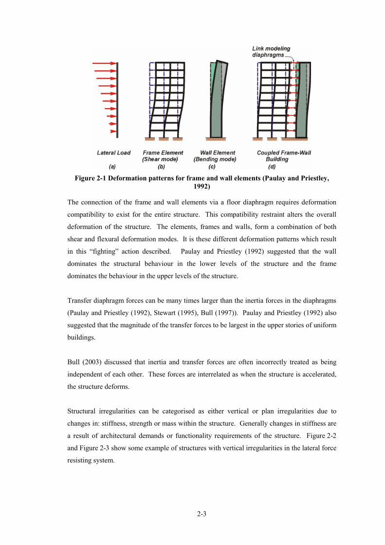
2�3

Figure 2(1 Deformation patterns for frame and wall elements (Paulay and Priestley,

1992)

The connection of the frame and wall elements via a floor diaphragm requires deformation

compatibility to exist for the entire structure. This compatibility restraint alters the overall

deformation of the structure. The elements, frames and walls, form a combination of both

shear and flexural deformation modes. It is these different deformation patterns which result

in this “fighting” action described. Paulay and Priestley (1992) suggested that the wall

dominates the structural behaviour in the lower levels of the structure and the frame

dominates the behaviour in the upper levels of the structure.

Transfer diaphragm forces can be many times larger than the inertia forces in the diaphragms

(Paulay and Priestley (1992), Stewart (1995), Bull (1997)). Paulay and Priestley (1992) also

suggested that the magnitude of the transfer forces to be largest in the upper stories of uniform

buildings.

Bull (2003) discussed that inertia and transfer forces are often incorrectly treated as being

independent of each other. These forces are interrelated as when the structure is accelerated,

the structure deforms.

Structural irregularities can be categorised as either vertical or plan irregularities due to

changes in: stiffness, strength or mass within the structure. Generally changes in stiffness are

a result of architectural demands or functionality requirements of the structure. Figure 2�2

and Figure 2�3 show some example of structures with vertical irregularities in the lateral force

resisting system.

2�4

Figure 2(2 The Sears Tower, Chicago Figure 2(3 Hotel Ukraina Moscow

Transfer forces also develop in structures with vertical irregularities. Examples of these

include podium structures and office structure with car parking beneath. Transfer forces are

expected to develop in podium structures due to the sudden change of stiffness between the

podium and tower of the structure. The podium laterally deforms significantly less than the

tower.

NZS1170.5 (Standards New Zealand., 2004) requires rational analysis to be carried out for

structures with mixed lateral force resisting systems. It is suggested that the analysis should

account for relative stiffness and location of elements to allocate the seismic resistance of

each element. The Standard does not give any further details on how to analyse or deal with

these structural systems.

2.1.3 DSDM Consortium

Research on reinforced concrete floor diaphragms is currently being undertaken by a

university research team which was formed to develop a seismic design methodology for

precast/prestressed concrete floor diaphragms (Fleischman et al., 2004). The research team

that is involved with this work is referred to as DSDM (Diaphragm Seismic Design

Methodology) Consortium. This research is jointly carried out by the: University of Arizona,

Lehigh University, University of California San Diego and input is also received from an

industry task group. This research includes: finite element analysis, full�scale experimental

tests to investigate reinforcing details and shaking table tests.

2�5

The objectives for this research were to develop an industry endorsed design methodology for

precast/prestressed diaphragms which include:

1. The forces, displacements and deformations for which the diaphragm should be

designed;

2. The diaphragm reinforcing details that can provide this performance;

3. The required stiffness of the diaphragm relative to the primary lateral force resisting

system.

At this stage no results have been published regarding this work.

2.1.4 Goodsir (1982)

Goodsir (1982) examined the inelastic seismic response of reinforced concrete frame�to�wall

structures. This work focused on the overall performance of frame�to�wall structures and the

actions induced in the floor diaphragm were not considered.

2.1.5 Beyer (2005)

Beyer (2005) carried out work which extended the study of Rutenberg and Leibovich (2002)

on the seismic response of walls of different lengths. The results of analytical predictions

from the direct displacement based design approach were compared to the results from non�

linear time history analyses. Beyer also extensively investigated the sensitivity of various

modelling assumptions used for the walls. The effects of the following structural responses

were considered in this study: displacements, drift, shear, bending moment demand, hysteretic

behaviour of walls, flexibility of floor diaphragms, shear stiffness of walls and modelling of

plasticity in structural walls. It was shown that modelling assumptions of: rigid floor

diaphragms, high shear stiffness of walls and lumped plasticity may lead to the overestimation

of the base shear demand of the smaller wall. The item which had the largest affect on the

response was related to the lumped plasticity assumption. This conclusion was determined by

comparing the results of lumped plasticity models to fibre element models. The sudden

change of stiffness associated with the lumped plasticity bi�linear hysteresis model caused

sudden changes in the displacements, which induced large transfer forces unlike the more

gradual change of displacements which occurs for a fibre model where the inelastic

deformation is distributed over a number of different fibres.

2.1.6 Sullivan et al. (2006)

Research carried out by Sullivan et al. (2006) on developing the direct displacement based

design method for frame�to�wall structures included a section on the floor behaviour in frame�

to�wall structures. The purpose of Sullivans work was to investigate the accuracy of the

2�6

newly proposed direct displacement based design methodology. The objectives of the

investigation of the floor behaviour were to:

− Validate the assumption of rigid floor diaphragms used in the analysis by determining

the effects of flexible floor diaphragms on the drift of the structure;

− Review the maximum forces in the floors of the structure;

− Ensure the performance of the capacity design procedure for the floor diaphragm

forces was acceptable.

The analyses carried out in Sullivan et al. (2006) work were modelled using RUAUMOKO3D

(Carr, 1981�2009c) with 7 different time history records. The floor diaphragm was modelled

using Giberson�beam elements, which allowed the flexural and shear stiffness of the floor to

be controlled. The moment of inertia of the slab was reduced to 25% of the gross section

stiffness to make allowance for cracking. The hysteretic model used in this analysis was the

Takada model and the damping used in the structure was tangent stiffness Rayleigh damping.

The results indicated that: there is no need to account for diaphragm flexibility when

performing displacement–based design of the frame�to�wall structures with length to width

aspect ratios of less than 1:3, the magnitude of shear forces in the floor diaphragm reduced

when the diaphragm increased in flexibility, the floor forces at three�quarters of the height of

the structure were found to be the smallest and the forces at the top of the structure were

found to be the greatest.

2.1.7 Priestley et al. (2007)

Research carried out by Priestley et al. (2007) discusses the incompatible deformation

patterns of walls of different lengths. This research identifies that yield displacement of walls

of different lengths is inversely proportional to the length of the wall. Therefore it was

concluded that the displacement ductility demands on the walls must differ since the

maximum response displacement of the structure will be the same for each wall. This

research also indicates that the long wall yield firsts which consequently results in a shear

transfer to the shorter wall.

2.1.8 Diaphragm Flexibility

Diaphragm flexibility is becoming more of an issue due to the types of structures being

designed in recent times. Precast concrete floor diaphragms are currently being constructed

with a reduced depth of topping slab or with no topping slab above the precast units. The

purpose of reducing or excluding the topping slab is to make the structure lighter and hence

2�7

reduce the inertial forces which may develop in the structure. The consequences of reducing

the weight and the thickness of the diaphragm are an increase in diaphragm flexibility of the

floor, a reduction in the connectivity of the diaphragm to the external frames and a reduction

in the shear transfer capacity within the diaphragm.

Stewart (1995) found that diaphragm flexibility can alter the magnitude of the actions induced

in the diaphragms. Further, Fleischman and Farrow (2002) found that highly flexible

diaphragms can change the dynamic properties of the structure.

Research carried out by Fleischman and Farrow (2002) showed that the dynamic force

distribution produced by a structure with a flexible diaphragm can significantly differ from

the force pattern given by the equivalent static analysis (ESA) method (first mode). The

research looked at the instantaneous effective centroid location of the force distribution for

the flexible diaphragms compared to the location of the centroid that is implied by the ESA

method; it was found that the flexible diaphragm centroid was slightly lower than the ESA

method centroid. This downward shift is said to be a result of higher mode effects and has the

potential to cause larger than expected diaphragm forces.

Diaphragm flexibility is defined in various international standards and codes (NZS1170.5

(2004), FEMA450 (2004) and Eurocode 8 (2004)) as a diaphragm where the maximum lateral

deflection is more than two times the value of the average inter�storey drift of the lateral force

resisting system. All of these Standards and Codes do not clearly identify the implications of

designing a structure with flexible diaphragms or provide clear guidance on how to design

structures with diaphragm flexibility.

FEMA450 (2004) assumes that diaphragm flexibility results entirely from local floor

properties. Fleischman and Farrow (2002) disagrees with this assumption, because it was

found that the local storey dependence for flexible diaphragms is only true for a certain

flexibility of the diaphragm relative to the lateral system. When the flexibility is large

diaphragm flexibility was found to dominate the dynamic response of the entire structure and

not just a localised part of the structure.

2.1.9 Higher Mode Affects

Higher mode affects can influence the magnitude of forces felt within a floor diaphragm and

can also change the response of the structure. Basically, higher modes excite the structure in

different deflection profiles and therefore can lead to a variety of forces forming in the

structure.

2�8

Research carried out by Rodriguez et al. (2002) identified that floor peak horizontal

accelerations were much greater than peak ground acceleration. The floor acceleration

magnification coefficients for Northridge earthquake were found to range from 1.1 to 4.6. It

was suggested that the amplification of accelerations could be due to higher mode effects.

2.1.10 Reviews of Previous Analytical Models

2.1.10.1 Damping

Various opinions exist on what type of damping model should be used in dynamic analysis.

The uncertainty surrounding damping forces is because damping forces are not simply

derived from equations of theoretical mechanics. The common types of damping are:

viscous, hysteretic and Coulomb. In some cases, for mathematical convenience, a

mathematical formulation describing damping is used in analysis. This type of damping

(viscous) is sometimes referred to as Rayleigh damping, which is one of the most commonly

used types of damping model in analysis.

Research carried out by Priestley and Grant (2005) suggests that tangent stiffness proportional

damping is a more realistic representation of damping for inelastic systems compared to

uniform damping. Concerns with this method related to high damping forces which can

develop in the structure due to the excitation of higher modes within the structure.

Carr (1997) provides recommendations for damping models to be used when carrying out

inelastic analyses. It is suggested that uniform damping should be specified for all modes. It

is also recommended that if a Rayleigh damping model is to be used then care must be taken

to ensure that high modes are not overly damped.

2.1.10.2 Rigid End Blocks

Rigid end blocks at the junction of members frame together account for extra stiffness of

members and the subassemblies of the members. The magnitude of any additional stiffness

will reduce as inelastic action develops in a structure due to: non�linear deformations in the

concrete, flexural and shear cracking in the joint, distortion of the joint, slippage or de�

bonding of the reinforcement and loss of cover concrete. In RUAUMOKO (Carr, 1981�

2009d) the assumed stiffness in the joint zone is constant and consequently allowance for the

degradation of the joint stiffness is not incorporated in the model. To determine if the loss of

stiffness of the joint should be incorporated into the model an investigation of the sensitivity

2�9

of the length of rigid end blocks on the magnitude of transfer forces was carried out and

described in Section A.1.3 of the Appendix.

The New Zealand Loadings Standard (Standards New Zealand, 2004a) states that rigid end

blocks for reinforced concrete frames should be taken as a proportion of the dimensions of the

beam�column joint. No details are provided regarding how large this proportioning should

be. Various researchers have commonly used the value 0.4 of the width of the column

member for the end block length of the beam member.

An issue with using rigid end blocks in RUAUMOKO is that they alter the length of the

member, resulting in the beam and column actions not being calculated at the beam or column

face of the member. The affect of this was considered by Flores Ruiz (2005).

Rigid Elements

Flexural springs

Rigid Elements

Rigid Elements

M/EIM/EIM/EI

AN

AL

YT

ICA

L

RE

PR

ES

EN

TA

TIO

N

RE

SU

LT

ING

C

UR

VA

TU

RE

Option A Option B Option C

Figure 2(4 Rigid end block method Flores Ruiz (2005)

Figure 2�4 represents the different rigid end block modelling options that were discussed by

Flores Ruiz (2005). Option A represents the case where the flexural stiffness of the member

was increased to represent realistic stiffness of the member. For this option the analytical

model would output the resulting curvatures at the centre line of the column which are

incorrect. Option B represent the case where the original beam stiffness was used, this

method also resulted in the curvatures being incorrectly output by the analytical model.

Option C is the method that Flores Ruiz (2005) came up with to get around the problem with

the response of the members not being calculated at the face of the beam or column member.

2�10

This option represents the stiffness of the beam column joint by the rigid elements and allows

the actions to be determined at the column face by incorporating flexural springs.

Comparisons were made between the magnitudes of transfer floor diaphragm forces for

identical structures with rigid end blocks modelled as Option A and Option C. The length of

the rigid end blocks, used for these models, for the beams and columns were equal to 0.4

times depth of the column and beam respectively. Comparisons between the results, shown in

Appendix A.1.3, indicated insignificant variations of the results for the two methods.

2.1.10.3 Foundation Modelling

Considerable research exists on the significance that foundation soil properties have on the

dynamic response of a structural system. Clendon (1985) carried out research on the

interaction between a foundation and a frame structure. This research indicated that generally

the forces of the frame reduced due to a lengthening of the fundamental period, T1, of the

frames, when allowance was made for foundation soils, but there was an increase in the

maximum levels of deflection of the frames.

Flexibility of the foundation alters the dynamic properties of structures and the fundamental

period of the system. Two mechanisms of interaction have been identified to develop

between the structure, foundation and soil components. These are inertial interaction and

kinematic interaction (Stewart et al., 1999). Inertial interaction results from the development

of inertia in the structure which causes the foundation to displace. Kinematic interaction

initiates due to the interaction between a stiff foundation and the soil. In this situation the stiff

foundation can alter the free field motion that is applied to the structure.

2.1.10.4 Shear Deformations

A paper by Kelly (2004) on non�linear analysis of reinforced concrete shear wall structures

uses a macro model to represent the response of a wall. This model is similar to a finite

element model, but it uses substantially larger elements to reduce the computational effort

required. Kelly modelled the shear behaviour of the wall by developing an empirical

hysteretic model, which was based on: experimental data from squat shear walls, the New

Zealand Structural Concrete Standard and requirements and recommendations from FEMA

guidelines for the evaluation of shear wall structures. This hysteresis model has a tri�linear

backbone curve which incorporates the following sections; elastic stiffness, cracked stiffness,

strain hardening, strength degradation, and residual strength. Figure 2�5 shows the proposed

hysteresis backbone curve.

2�11

Shear strain

Sh

ear

str

ess (

kP

a)

Residual Strength

1/222

1/133

1/50

VC

VC+VS

VC+1.25VS

Figure 2(5 Backbone curve for concrete shear wall (Kelly, 2004)

The symbols, Vc and Vs in this figure refer to concrete and components of shear strength in a

wall. It can be clearly seen that the strength degradation in the back bone curve shown in this

figure increases with increasing strain or ductility of the structure.

Priestley et al. (2007) models shear deformations using an approach which assumes bi�linear

flexural force assumption. The method is based on 3 stages. The first stage is when the

member is elastic prior to shear cracking, the second stage considers the member when it is

elastic after shear cracking and the final stage corresponds to the ductile phase.

Priestley et al. (2007) describes that in the post yield phase, the concrete compression struts

within the plastic hinge region continue to soften, which in turn causes the shear deformations

to increase. It is also recommend, that because rational computation of the shear deformation

is difficult to determine, the shear deformation should be increased in proportion to the

flexural deformation after yield.

2.1.10.5 Plastic Hinge Element

An analytical ductile reinforced concrete plastic hinge beam element was developed by

Peng (2009). This element was made up of a variety of springs which represent the

reinforcing steel, shear deformations, cover and core concrete in the hinge element.

Comparisons of this element with experimental results indicated that this element was capable

of predicting the flexure, shear, axial and elongation response of a ductile plastic hinge.

2�12

2.1.11 Summary of Literature Review

In this research, one of the aims was to develop a floor diaphragm “desktop” static force

design method. To do this, an understanding of the different types of forces (inertial and

transfer), which typically develop in floor diaphragms, is required. Reviews of the literature

indicate that there is reasonable understanding around inertial forces but not such a good

understanding relating to transfer forces. This chapter of research will investigate the trends

associated with the magnitudes and distributions of transfer forces.

The findings from this literature search provides suggestions for different analytical

modelling parameters that should be used in analyses and also indicate some parameters that

could be sensitive to the presences of transfer forces. Summaries of these are provided in the

following paragraphs.

Priestley et al. (2007) discussed that two walls connected together of different lengths can

yield at different times resulting in a lateral force transfer developing between the walls.

These walls are likely to have different displacements, due to yielding at different times, and

therefore compatibility transfer forces would also be expected to develop. Walls of different

lengths will be included in this study.

The outcomes from Beyers (2005) work indicated that a lumped plasticity assumption,

representing the plastic hinge behaviour in walls, may affect the magnitudes of compatibility

transfer forces. In the initial analytical dual structure models used to determine some of the

fundamental trends relating to transfer forces, the soil properties, shear deformations of the

wall elements and the distributed plastic hinge model, were not included. The literature

indicated that these parameters could possibly affect the magnitudes of transfer forces. A

sensitivity study, detailed in Chapter 3, was later carried out to determine the sensitivity of

these parameters to transfer forces.

Research carried out by Sullivan et al. (2006) reported some vertical distribution of forces

which developed in dual structures. These force distributions were compared to the

distribution of forces found in the analyses carried out in this research.

It is expected that transfer forces will dominate for the first few inelastic modes of response of

the structure and the inertial forces will dominate for the higher modes of the structure. A

simple study on the magnitude of transfer forces for different dynamic modes was carried out

in Section 2.3.1.

2�13

2.2 Description of Analytical Models

A variety of different structural models were developed for this research to investigate the

trends of compatibility transfer forces which develop in floor diaphragms of multi�storey

structures. Numerical integration time history analysis was carried out for each of these

models. These models were 2�dimensional analytical models with consideration for the

inelastic response of the structure. A rigid foundation was assumed for the analyses carried

out in this section. The affects of foundation flexibility were considered in the sensitivity

study described in Chapter 3.

The variations of the analytical structural models, which were incorporated in this study, on

the trends of transfer forces included variations of:

− Frame�to�wall stiffness ratio;

− Design ductility of the structure;

− Strength of the floor diaphragm;

− Stiffness of the floor diaphragm;

− Height of the structure;

− Flexibility of the structure;

− Seismic region;

− Type of structural system: podium structures and walls of different lengths.

The general parameters used for each of these analytical models are provided in the following

sections. Specific parameters relating to a specific variation, such as the variation in the

frame�to�wall stiffness ratio, are provided at the start of the relative results section.

Compatibility transfer forces are referred to as “transfer forces” in subsequent sections.

2.2.1 Analysis Program

The analytical program that was used for this research was RUAUMOKO (Carr, 1981�

2009d). The initial version of this program was developed in 1981, since this time many

additional features have been added and are still being added to this program. RUAUMOKO

is a numerical integration time history analysis program which can perform: two�dimensional

and three�dimensional, static, dynamic, elastic and inelastic analyses. This program provides

various modelling options to carry out a variety of different types of analyses, such as: static

analysis, dynamic time history analyses, pushover analyses and ground displacement history

analyses. The options available in RUAUMOKO provided flexibility in terms of: how the

mass is modelled, the type of damping model used in the analysis, the type of member used,

2�14

the stiffness, strengths and hysteretic properties for each member, the type of input motion or

external forces which act on the structure, P�delta effects, foundation modelling and external

forces applied to the structure during dynamic analysis.

RUAUMOKO has an extensive range of hysteretic models available to model a variety of

types of inelastic action in various situations. This program was chosen for this research as a

result of its capacity to perform non�linear time history analyses and its flexibility in terms of

the choice of modelling parameters.

2.2.2 Structural System

Different structural systems with different vertical lateral force resisting systems were

analysed in this study. For the majority of the research presented in this section, frame�to�

wall structural systems were used; other analytical models with different structural systems

including, podium systems and wall�to�wall systems were included for minor sections. The

relative behaviour between the seismic resisting systems, of the structure, was represented in

two dimensions. The seismic systems were connected via a rigid pin spring element which

represented the floor diaphragm. This element was elastic for the majority of the analyses,

the affects of inelasticity of the floor diaphragm were considered in Section 2.3.5.

(a) Plan View (b) Side View

Figure 2(6 Model used to investigate transfer forces in the floor diaphragm

Figure 2�6 indicates the geometry of the frame�to�wall structural model. For the frame�to�

wall structural system, the frame consisted of 3 bays with a span of 7m, the walls were

400mm thick with varying lengths and the inter�storey height was 3.6m. Specific geometry

parameters such as the frame to wall stiffness ratios are provide in the results section for each

study in Section 2.3.

The thickness of the floor diaphragm, including both the topping and precast floor thickness,

was 390mm. Different floor diaphragm thicknesses were analysed to determine the affect on

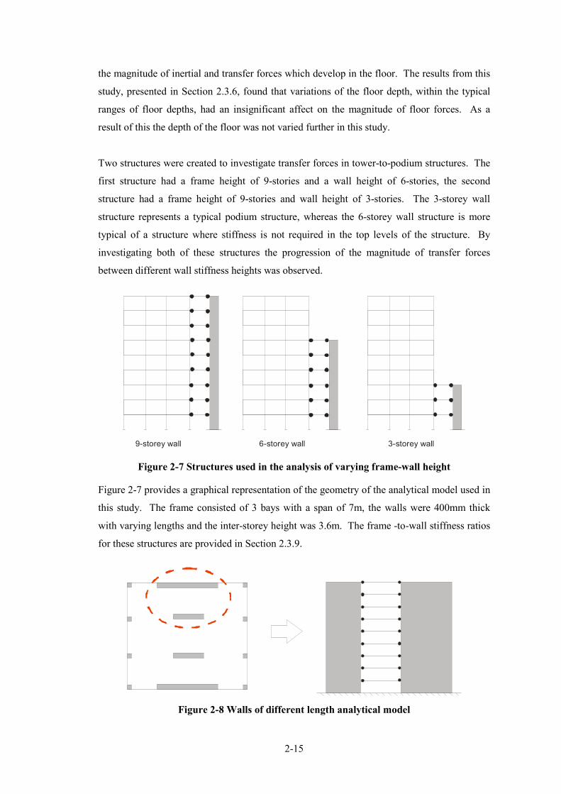
2�15

the magnitude of inertial and transfer forces which develop in the floor. The results from this

study, presented in Section 2.3.6, found that variations of the floor depth, within the typical

ranges of floor depths, had an insignificant affect on the magnitude of floor forces. As a

result of this the depth of the floor was not varied further in this study.

Two structures were created to investigate transfer forces in tower�to�podium structures. The

first structure had a frame height of 9�stories and a wall height of 6�stories, the second

structure had a frame height of 9�stories and wall height of 3�stories. The 3�storey wall

structure represents a typical podium structure, whereas the 6�storey wall structure is more

typical of a structure where stiffness is not required in the top levels of the structure. By

investigating both of these structures the progression of the magnitude of transfer forces

between different wall stiffness heights was observed.

9�storey wall 6�storey wall 3�storey wall

Figure 2(7 Structures used in the analysis of varying frame(wall height

Figure 2�7 provides a graphical representation of the geometry of the analytical model used in

this study. The frame consisted of 3 bays with a span of 7m, the walls were 400mm thick

with varying lengths and the inter�storey height was 3.6m. The frame �to�wall stiffness ratios

for these structures are provided in Section 2.3.9.

Figure 2(8 Walls of different length analytical model

2�16

Transfer forces were investigated for wall�to�wall structures. The analytical model used for

this wall�to�wall study consisted of two walls, of different lengths, joint by stiff links which

represented the floor diaphragm. Further details relating to the lengths of the walls are

provided in the results in Section 2.3.10.

Tremayne and Kelly (2005) carried out time history analysis to investigate the time history

record scaling method presented in the New Zealand Loadings Standard NZS1170.5 (2004).

This analysis included, 8 prototype moment frames and shear wall buildings. These buildings

were 6 and 12 stories high and located on sites in Wellington and Auckland. The drift limits

and fundamental periods of these structures were used as guidance to ensure realistic

structures were developed in this study. The lateral force resisting systems for the structures

used in Tremayne and Kellys study were different to the structures used in this research. The

structural systems of the buildings in Tremayne and Kelly’s study were wall and frame

elements that were perpendicular to each other, whereas the frame and wall elements were

parallel to each other for this research.

2.2.3 General Parameters

The mass matrix, in the analytical model, was represented as a lumped mass matrix where the

surrounding mass of the structure was lumped at the nodes in the analytical model. Large

displacement effects were included in the analysis to account for the additional overturning

effects that can occur within a structure. The time step used for the analyses was 0.002s. A

study was carried to determine that this step size led to acceptable accuracy, the results from

this study are presented the Appendix in Section A.1.4.

Damping is a parameter that is very structure specific. There are various types of damping

models which have been developed to represent different structural damping actions. Some

of the different damping models include; Viscous Damping, Hysteretic Damping, Coulomb

Damping and Proportional (Rayleigh) Damping. Engineers have a variety of different

opinions on what damping model is the best. The Proportional Rayleigh Damping model is

the most commonly used. A study was carried out to determine the sensitivity of some of

these damping models to the magnitudes of floor diaphragm forces. A description and the

results from this study are provided in the Appendix in Section A.1.2. The results from this

study indicated variations of the magnitudes of damping forces of around 2% of the total floor

diaphragm forces. The damping model that was used in this research was a Rayleigh

damping model which used the tangent damping matrix as a secant damping matrix. For this

model 5% damping was applied to the 1st and 9

th dynamic modes of the structure.

2�17

The magnitudes of inertial forces in the floor diaphragms were obtained by multiplying the

mass by the total accelerations of the floor from the analyses. The magnitude of transfer

forces in the analytical model were obtained by subtracting the inertial forces from the total

floor forces for each time step. This was done wherever transfer forces were obtained.

2.2.4 Members

Column members of the structures were initially modelled as reinforced concrete members

with an axial force moment interaction yield surface. A diagram of the axial force�moment

interaction yield surface used to model the column interaction is provided in Figure 2�9.

In later models, the plastic hinge behaviour of the columns was modelled separately with the

modified plastic hinge element that is described in Section 2.1.10.5. Beam members were

modelled using beam elements where axial force moment interactions are not included in the

response of the member. The beam elements were modelled using Giberson one component

members and the wall members were initially model as two�component beam members and

later modelled using a wall plastic hinge element. The wall plastic hinge element was used to

represent the wall elements in the sensitivity study that is described in Chapter 3.

P (Axial force �

negative)

P , MB B

2/3.P , MB 1B

1/3.P , MB 2B

MO

Pyt

Pyc

Figure 2(9 Concrete beam(column yield interaction surface (Carr, 1981(2009b)

In this figure, Pyc, refers to the axial compression yield force, Pb, represents the axial

compression force at a point b, where, b, is any point on the curve, Mb, refers to the yield

moment at point, b, Mo, represents the yield moment at zero axial load and, Pyt, refers to the

axial tension yield force.

2�18

The floor diaphragm was represented by an elastic spring element in the analytical model.

The affects of allowing inelasticity in this element were considered in Section 2.3.5. The

stiffness of the spring element was made to represent the typical stiffness of a floor diaphragm

with large in�plane stiffness and negligible out of plane stiffness which represented the shear

transfer action which typically occurs in floor diaphragms. This spring element adequately

represents the floor diaphragm as long as the transfer of forces within the floor is

predominantly by shear transfer and not flexure.

Effective section properties were assumed in the analysis to account for the stiffness

degradation which occurs in the members due to flexural cracking of the section. The

effective section properties reported in New Zealand Concrete Structures Standard

NZS3101 (2006) were used. The effective axial stiffness of the floor diaphragm was taken as

0.25 of the elastic stiffness as suggested by ACI Committee 318 (2008).

The response of structures to earthquake motion requires the use of realistic stiffness

degradation models. The hysteresis model employed to represent the inelastic action in the

frame and the wall members was the Revised Takeda Model (Takeda et al., 1970). This

model is based on results from a number of medium sized reinforced concrete members with

low to medium axial forces applied. These columns were subjected to cyclic loading. This

model was used because it represents typical hysteretic behaviour of reinforced concrete

members.

2�19

Displacement

Φβk

Force

ko

dy

YP

FCRP.YP

YN

FCRN.YN

Φko

αko

Φrko

Ddu

Arko

k (dy/du)o

γ

Figure 2(10 Revised Takada hysteresis (Carr, 1981(2009b)

Where YP and YN refer to the tension and compression yield forces, ko, is the initial stiffness,

α, is the positive cracking to yield bi�linear factor, β is the negative cracking to yield bi�linear

factor, r, is the positive yield to ultimate bi�linear factor, dy ,and, du, are the yield and ultimate

displacements, Ф, is the compression to tension stiffness ratio and, γ, is the unloading power

factor.

The bi�linear and unloading parameters required to define the revised Takada hysteresis loop

were obtained from the moment curvature analysis that was carried out for each member by

the moment curvature analysis program RESPONSE (Bentz E. C., 2002). The other

parameters that were used to define the revised Takada hysteresis loop are provided in

Table 2�1.

Table 2(1 Parameters to define revised Takada hysteresis loop

Positive cracking to yield bi�linear factor, α 0.6

Negative cracking to yield bi�linear factor, β 0.6

Unloading power factor, γ 0.4

Ratio of compressive to tensile stiffness, Ф 1.0

Cracking action as ratio of positive yield, FCRP 0.3

Cracking action as ratio of negative yield, FCRN 0.3

2�20

The strengths of the members used in the analytical models were obtained by carrying out a

static analysis in RUAUMOKO. The Equivalent Static Analysis (ESA) method given in New

Zealand Loadings Standard (2004a) was used to determine the seismic base shear for the

structure. The majority of the structures were designed for the Wellington region of New

Zealand with a design structural ductility of 3 (variations of this are reported in Section 2.3 on

the analysis and results for each model). The calculated base shear forces were then

distributed according to the New Zealand Loadings Standard (2004a) and statically applied to

the structure. From the statically applied loads, the moments and shears in each of the

columns and beams were obtained. These values were initially roughly checked using hand

calculations and approximating the location of the inflection point per column, via the Muto

method (Muto, 1974), and calculating the moment from the distributed shears. Capacity

design, as required by the New Zealand Loadings Standard, was carried out to ensure a strong

column�weak beam mechanism would form in the structural system. For these analyses the

member strengths were based on nominal strength values which were determined from lower

characteristic reinforcement strengths defined in (Standards New Zealand, 2006). The yield

surfaces for each member were calculated using modified compression field theory to

determine capacity of a section (Bentz and Collins, 2002).

There are a variety of different methods, suggested in various publications, to calculate the

effective plastic hinge lengths of different elements in a structure. Comparisons were made

between the floor forces obtained when the effective plastic hinge lengths were determined by

the two different methods described in Paulay and Priestley (1992) and Priestley et al (2007).

The results from this study are given in the Appendix in Section A.1.1. This study indicated

that the floor diaphragm forces were not significantly sensitive for these two plastic hinge

methods. The plastic hinge length prediction method that was used in these analyses was the

model presented in Priestley et al (2007). This model has been used as it is the most

comprehensive model. It accounts for inelastic action affects, strain penetration and tension

shift affects on the length of the hinge.

During an earthquake, the stiffness of beam column joints in a structure degrade due to

inelastic behaviour such as, cracking of the concrete and yielding of the bars within the joint.

In analytical modelling, the effects of stiffness degradation of the joint are not typically taken

into account. To determine how sensitive the magnitudes of floor diaphragm forces were to

the size of the rigid end blocks, comparisons were made to floor force results for structures

with different sized rigid end block which represented different levels for degradation of the

joining. This study is described in the Appendix in Section A.1.3. The results from this study

2�21

indicated that floor diaphragms forces were not sensitive to different rigid end block lengths.

Therefore, rigid end blocks with a value of 0.4 times the depth of the column for the beams

and 0.4 times the depth of the beams for the column were used for the analytical models in

this study.

2.2.5 Weights and Loads

The weights used in the analysis are based on the values supplied in Table 2�2.

Table 2(2 Weights of elements

Hollow core floor 300kg/m2

Thickness of topping slab 90mm

Density of concrete 23.5kN/m3

Super imposed dead load 1.3kPa

Curtains walls and glazing 0.4kPa

Live Load 3kPa

Reduction factors were used to determine the appropriate live load for the structure according

to the New Zealand Structural Loadings Standard. The weight was found per area of the

structure and then distributed in proportion to the area attributed to the node. The weights of

the columns were lumped at the adjacent upper and lower nodal points in the analytical model

as indicated in the general layout of the nodes for the 9�storey structure shown in Figure 2�11.

2�22

Figure 2(11 Layout of nodes for 9(storey structure

2.2.6 Time History Records

The New Zealand Loadings Standard, NZS1170.5 (Standards New Zealand, 2004a) requires

that at least 3�time history records be used when carrying out non�linear time�history records.

Twelve time history records (six records in the North�South and six records in East�West

direction) were employed to investigate the trends of inertial and transfer forces. These

records were obtained from the institute of Geological and Nuclear Sciences (GNS) and from

Pacific Earthquake Engineering Research Centre (PEER) Strong Motion Database (University

of California, 2005).

It is paramount when choosing time history records that the record is representative of the site

of interest. Considerations must be given to the: soil type, faulting types, rupture depth,

duration, frequency and the location of the site compared to location of the fault. Generally

there are not enough genuine time history records recorded at the site of interest to conduct a

respectable number of time history analyses. Therefore the characteristics of world�wide

records are generally selected to match the characteristics of the site of interest. Due to the

randomness of earthquake excitation, the New Zealand Loadings Standard require that more

than three time history record are employed when carrying out time history analysis, they also

require the records are scaled to match the site of interest.

2�23

The records chosen for the majority of research in this section were records with similar

motion characteristics to that expected of a seismic event in the Wellington region in New

Zealand. Wellington was chosen for this study as it is a high seismic region in New Zealand.

There are three major types of possible fault motion that are likely to occur in Wellington

(McVerry, 2003). These are:

− Strong�forward directivity motion caused by the possible rupture of the Wellington

fault (active right lateral strike�slip fault);

− Near�neutral directivity due to rupture on the Wellington fault;

− Motion which is related to a large subduction zone type event.

The earthquake records chosen generally represent these identified motion characteristics for

Wellington.

Strong directivity effects would be associated with the Wellington fault rupturing near

Kaitoke and propagating southwards, this would result in maximum directivity effects in

central Wellington. The 1992 Landers, California earthquake recorded at the Lucerne station

was recommended by Somerville et al. (1997) as it contains characteristics of large directivity

effects. Large directivity effects are generally related to earthquakes which have large

velocity pulses such as the Lucerne record. The Lucerne record was obtained from the PEER

Strong Motion Database (University of California, 2005).

The Wellington Central Business District is located in a high seismic zone which could

potentially sustain a seismic ground motion with non�directivity affects. The 1999 Kocaeli,

Turkey earthquake recorded at the Izmit station was used to represent this type of ground

motion with no directivity. The Kocaeli ground motion record was recorded close to the

epicentre (7.2 km) and therefore the directivity effects did not develop. Rathje et al. (2000)

considered the acceleration response spectra for a variety of records located at various

distances from the epicentre. The large acceleration peaks that are typically present in ground

motion records with significant directivity affects were not present in the Izmit ground motion

record. This record was obtained from the PEER Strong Motion Database.

A subduction zone type event is considered a possible threat to the Wellington region as the

Hikurangi subduction zone is located on the eastern coast of the North Island, which is in the

vicinity of the Wellington region. The Pacific tectonic plate is thrusting under the Australian

plate in this subduction zone. Scientists believe that this subduction zone is capable of

producing an earthquake of magnitude 7.5�8.3. The 1985 Michoacan Mexico Cocos Plate

subduction zone record at the La Union station was 8.1 in magnitude; this event has been

2�24

recommended as an example of a great subduction zone event (McVerry, 2003). This record

was obtained from the GeoNet Strong Motion Database (GeoNet, 2008).

The 1940 Imperial Valley, USA earthquake recorded at El Centro station was chosen as a

time history record for this study. The El Centro record was one of the first recorded ground

motion record. It has been used numerous times in research, so this record was used as a

benchmark. It allows comparisons to be made between the results from the other time history

records and the response of other types of structures. This record was obtained from the

GeoNet Strong Motion Database.

The 7.8 magnitude, 1985 Chile earthquake recorded at Llolleo station resulted from rupture

along the Chilean subduction zone. This record was incorporated as it is a subduction zone

event, again representing a possible rupture along the Hikurangi subduction zone. This time

history record is also of a magnitude that is similar to the expected magnitude of a subduction

type event in the Wellington area. This record was obtained from the GeoNet Strong Motion

Database.

The 1978 Tabas, Iran earthquake recorded at the Tabas station was associated with 85km of

surface rupture along a previously unknown quaternary thrust fault (Tabas fault) (Berberian,

1978). This record has been used as parts of the Hikurangi subduction zone could rupture due

to possible thrusting action (Reyners et al., 1999). This record was obtained from the GeoNet

Strong Motion Database.

Information on each of the ground motion records that were chosen for this study are

summarised in Table 2�3. The North and South components recorded at each of the stations

were used for the analyses of Wellington buildings carried out in the research.

Table 2(3 Information about the earthquake used in the regular analysis

Ref Location Station Fault type Date Magnitude

1 Landers, California Lucerne Strike�slip 28 June 1992 7.3

2 Kocaeli, Turkey Izmit Strike�slip 17 August

1999 7.4

3 Michoacán,

Mexico La Union

Subduction

zone

19 September

1985 8.1

4 USA, El Centro,

Imperial Valley El Centro Strike slip 19 May 1940 7.0

5 Chile Llolleo Subduction

zone 3 March 1985 7.8

6 Iran, Tabas Tabas Thrust 16 September

1978 7.2

2�25

2.2.6.1 Scaling

These time history records were scaled according to the New Zealand Loadings Standard

(Standards New Zealand, 2004a) for each analyses to match the site specific design spectra.

For design purposes the scaling consists of two parts. The first part requires the difference

between the earthquake record response spectra and the design response spectra to be

minimised over the range of 0.4T1 to 1.3T1, where T1 is the fundamental translational natural

period of the structure. The difference between the two response spectra is calculated by

Equation 2�1 below. Where, k1, is the record scale factor, SAcomponent, refers to the spectral

acceleration of the time history record and SAtarget is the spectral acceleration of the design

response spectra.

=

ett

component

SA

SAkdifference

arg

1ln Equation 2(1

This is carried out by multiplying the earthquake record by a factor, k1, which minimises the

differences. The second part of scaling a time history record requires that at least one of the

earthquake records is larger than the response spectra at every point within the time band

given above. This constraint is satisfied by multiplying all of the earthquake records by a

factor, kt, until at least one of the earthquake records is greater than the elastic response

spectra.

Where the time history method is used for design the individual record scale factors are

obtained by multiplying the k1 factor by a kt factor. The kt factor is a factor that ensures, for

every period over the range of interest, the ground motion response spectra of at least one

record is above the design response spectra. However in this project only the k1 factor was

used to scale the time history records for these analyses to avoid unnecessary conservatism in

the results. The scale factors obtained from scaling the earthquake records are given in each

section of this report as they are specific to the fundamental period of each structure.

The Geology of the Wellington Area map (geological map 22) produced by GNS (Begg and

Mazengarb, 1996) was used to obtain some information about the soil properties in this area.

This information indicated that a variety of soil deposit lay beneath the Wellington CBD area.

The deposits in the Lambton Quay/water front zone are marginal marine sediments, further

inland in the CBD area the deposits are alluvium, silt, peat and loess. This information in

combination with information about the depth of the soil in the Wellington CBD area

(between 0�60m) allowed the site class to be identified. The site subsoil class used to scale the

time history records was shallow soil, or site class C.

2�26

2.3 Analyses and Results

The effects of varying: frame�to�wall stiffness ratios, structural ductility, frame�to�wall

connection strengths, structural heights, level of seismicity, and structural layouts on the

magnitude of transfer and inertial forces in floor diaphragms were investigated in this section.

To determine the trends that are associated with floor diaphragm forces, a number of static

and dynamic analyses were carried out. Simple modal analyses were performed to determine

some fundamental trends relating to transfer forces; these results are described in

Section 2.3.1.

Time history analyses were then carried out to determine the time dependent behaviour of the

forces which develop in floor diaphragm. A range of analyses investigating the affects of

variations of frame�to�wall stiffness ratios, structural ductility, flexibility of the structure,

variations of floor diaphragm strength and stiffness and different heights of the structures

were carried out using analytical models with the frame�to�wall structural system.

Descriptions of the frame�to�wall model that were used for these analyses are provided in the

below paragraphs.

Time history analyses were carried out to investigate the magnitudes of floor diaphragm

forces for structures designed for low seismic regions. For this analysis a structure located in

the Auckland region was designed. Details of this structure and the results from this study are

provided in Section 2.3.8.

Different structural systems were investigated, using time history analysis, to determine how

different structural systems affect floor diaphragm forces. Podium structures and structures

with different length walls were included in this study. Descriptions of these structures and

the results from this study are provided in Sections 2.3.9 and 2.3.10.

A further study was carried out to investigate whether transfer and inertial forces could be

determined separately and then added together. Comparisons were made between adding

these forces together separately and the forces obtained from time history analysis. A

description of this analysis and the results is provided in Section 2.3.11.

The parameters that were used in the frame�to�wall model that was used in the analyses for

Sections 2.3.1 through to Section 2.3.7 are provided in the following paragraphs.

2�27

The frame�to�wall stiffness was varied to investigate the influence of relative stiffness of the

vertical lateral force resisting system on the magnitude of the forces which develop in the

floor. The variation of stiffness between the frame and wall elements was measured by

determining the relative ratio of stiffness for the frame and the wall. The stiffness of the

frame and the stiffness of the wall were determined separately by carrying out pushover

analyses. From these stiffness values the ratio between the stiffness of the frame and the wall

components (frame�to�wall stiffness ratio) was determined. The frame�to�wall stiffness ratios

that were investigated in this study were; SR1:0.85, SR1:1.23, SR1:69 and SR1:2.58. These

ratios were chosen as they represent a realistic range of stiffness ratios for frame�to�wall

structures. The member sizes for the 9�storey structures, which correlated to these different

stiffness ratios, are provided in Table 2�4. The properties for the 9�storey structures have only

been described here as these structures have been used for the majority of the analyses. The

affects of different heights of the structure on the magnitudes of diaphragm forces was

considered in Section 2.3.7, the parameters fro these structures were provided in this section

with the results.

Table 2(4 Geometries of the members of the models for the different stiffness ratios

Stiffness ratio Beam Column Wall

1:0.85 0.9m by 0.6m 1.2m by 1.2m 9.45m by 0.40m

1:1.23 0.9m by 0.6m 1.0m by 1.0m 10.05m by 0.40m

1:1.69 0.9m by 0.6m 0.85m by 0.85m 10.53m by 0.40m

1:2.58 0.9m by 0.6m 0.70m by 0.70m 11.10m by 0.40m

The fundamental translational period of the 9�storey analytical frame�to�wall structure model

was 0.57s. To ensure each of the structures with different stiffness ratios had the same

dynamic properties, the elastic fundamental translational period of each of these structures

was kept constant. An investigation on the affects of structures with different overall

flexibility was carried out, descriptions of these structures and the results from this

investigation are provided in Section 2.3.4.

The earthquake scale factors that were used for the time history analysis for the 9�storey

structure are provided in Table 2�5.

2�28

Table 2(5 Scale factors for the earthquake records for 9(storey structure

Record Component k1 9(storey

Lucerne North 1.02

Lucerne South 1.40

Izmit North 1.84

Izmit South 1.57

La Union North 1.69

La Union South 1.98

El Centro North 0.96

El Centro South 1.40

Llolleo North 0.82

Llolleo South 0.56

Tabas North 0.49

Tabas South 0.42

2.3.1 General Concepts

To obtain a general understanding of transfer forces both modal and pushover analyses were

carried out.

Reviews of the literature indicated that transfer forces can develop in floor diaphragms due to

compatibility constraints, imposed by the connection with the floor diaphragm, between

lateral force resisting elements which have different fundamental deformation patterns; such

as frames and walls for example. This indicates that transfer forces are deformation

controlled, therefore it is expected that transfer forces will be the dominant force for the lower

dynamic modes of the structure and inertial forces will be dominant for the higher modes of

the structures. To investigate this, modal and pushover analyses were carried out to determine

the contribution that different dynamic modes had to the magnitudes of transfer forces.

The 9�storey analytical frame�to�wall model with a stiffness ratio of SR 1:1.23 designed for

structural ductility of 3 was used for this study. This structure was chosen as it represents a

typical medium rise dual structure. Only one structure was considered for this initial study to

allow initial trends to be identified. The affects of variations of: stiffness, strength and height

are provided in the Sections 2.3.2 to 2.3.7.

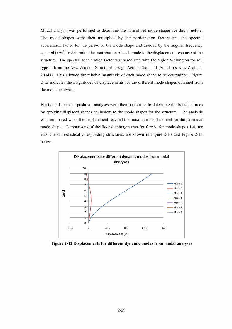
2�29

Modal analysis was performed to determine the normalised mode shapes for this structure.

The mode shapes were then multiplied by the participation factors and the spectral

acceleration factor for the period of the mode shape and divided by the angular frequency

squared (1/ω2) to determine the contribution of each mode to the displacement response of the

structure. The spectral acceleration factor was associated with the region Wellington for soil

type C from the New Zealand Structural Design Actions Standard (Standards New Zealand,

2004a). This allowed the relative magnitude of each mode shape to be determined. Figure

2�12 indicates the magnitudes of displacements for the different mode shapes obtained from

the modal analysis.

Elastic and inelastic pushover analyses were then performed to determine the transfer forces

by applying displaced shapes equivalent to the mode shapes for the structure. The analysis

was terminated when the displacement reached the maximum displacement for the particular

mode shape. Comparisons of the floor diaphragm transfer forces, for mode shapes 1�4, for

elastic and in�elastically responding structures, are shown in Figure 2�13 and Figure 2�14

below.

0

1

2

3

4

5

6

7

8

9

10

-0.05 0 0.05 0.1 0.15 0.2

Lev

el

Displacement (m)

Displacements for different dynamic modes from modal

analyses

Mode 1

Mode 2

Mode 3

Mode 4

Mode 5

Mode 6

Mode 7

Figure 2(12 Displacements for different dynamic modes from modal analyses

2�30

-4000 -2000 0 2000 4000

1

2

3

4

5

6

7

8

9

Transfer force

Le

ve

l

Transfer forces in the elastic

structure for different mode shapes

Mode 4

Mode 3

Mode 2

Mode 1

Figure 2(13 Transfer forces in the elastic structures for different mode shapes

-4000 -2000 0 2000

1

2

3

4

5

6

7

8

9

Transfer force

Le

ve

l

Transfer forces in inelastic structure

for different mode shapes

Mode 1

Mode 2

Mode 3

Mode 4

Figure 2(14 Transfer forces in the inelastic structures for different mode shapes

The results from the modal and simple pushover analyses, for the 2 dimensional 9�storey

building with stiffness ratio of SR1:1.23 and structural ductility of 3, showed the following

trends:

− The displacements are much larger for mode 1 compared to other modes, indicating

that transfer forces reduce with increasing modes;

2�31

− For the elastically responding structure, mode 1 resulted in the largest transfer forces

compared to the higher modes. The maximum values for mode 2, mode 3 and mode

4 were 77%, 41% and 17%, respectively of the maximum value for mode 1;

− For the inelastically responding structure the forces are again shown to be largest for

mode 1 and smaller for the higher modes. The maximum floor forces in mode 2, 3

and 4 were 66%, 47% and 19% of the maximum floor forces observed to develop for

mode 1;

− For the elastic structure, the distribution of transfer forces for mode 1 indicated

compression forces in the floor diaphragms link elements which represent the average

floor diaphragm forces for all levels apart from level 9 were tension forces were

observed to develop. These tension forces are thought to be due to the variation of

relative stiffness between the frame and the wall element with height of the structure.

This is illustrated in Figure 2�15;

− For the inelastic structure the distribution of transfer forces for mode 1 indicated net

compression forces for level 1, 6�8 and tension forces for levels 2�5 and 9. This

pattern of forces is different to the elastic results due to the development of plastic

hinges in the beams in the upper levels;

− The distributions of transfer forces seem to be similar for the higher modes. This is

possibly because inelastic behaviour typically affects the fundamental mode and not

higher modes (Rodriguez et al., 2002). This is also explains why a large reduction of

transfer forces occurs between elastic and inelastic for mode 1.

Deformation

Hei

gh

t

Frame

Wall

Figure 2(15 Comparisons between fundamental deformation patterns for frame and

wall element

The trends obtained from this study provide some interesting results. These results indicate

that the magnitudes of transfer forces are expected to decrease with increasing modes as these

2�32

are compatibility displacement driven. The magnitudes of transfer forces for modes 3 and 4,

of the order of 47% and 19% respectively of the magnitude of transfer forces for mode 1,

developed due to displacements of the order of 1�3mm. Displacements of this size are likely

to be affected by redistribution and cracking within the floor diaphragm and the lateral force

resisting elements. As a consequence of this the magnitudes of transfer forces for these

higher modes are likely to reduce as demonstrated for the 9�storey case study Figure 2�13 and

Figure 2�14. The amount of redistribution and cracking which develops and the affect that it

has on the transfer forces is unknown. It is not expected to result in zero displacement and

consequently zero transfer forces due to interactions from the inertial forces and other

dynamic modes occurring in the structure at the same time which could result in different

displacements. Due to this complex behaviour, non�linear time history analyses, on a range

of structures, has been carried out in the following sections to determine further trends

associated with transfer and inertial forces. Time history analysis will allow the interaction

between transfer and inertial forces to be considered.

2.3.2 Variations of Stiffness Ratio

This section investigates the affects that variations in the frame�to�wall stiffness ratios have

on the magnitudes of forces which develop in the floor diaphragm. The 9�storey structures,

designed for structural ductility of 3, with frame�to�wall stiffness ratios of SR1:0.85,

SR1:1.23, SR1:69 and SR1:2.58 were used for this analytical study.

2.3.2.1 Transfer Floor Forces

A selection of the results from the time history analysis for different frame�to�wall stiffness

ratios are shown in the Figure 2�16 to Figure 2�18. These figures show the magnitudes of

transfer forces that were observed to develop in the floor diaphragms for levels 1, 2 and 9 of

the structure. These levels were found to be the most critical in terms of the magnitude of

transfer forces which developed in the structure. The results shown in Figure 2�16 to

Figure 2�18 indicate the affects of different frame�to�wall stiffness ratios on the magnitude of

transfer forces. The transfer force component of the total floor force has been shown to

indicate the magnitudes and trends associated with transfer forces alone. It should be noted

that these forces should not be dealt with separately during the design process as they act

simultaneously with inertial forces, as previously discussed.

2�33

-500

-400

-300

-200

-100

0

100

200

300

400

500

600

0 10 20 30 40

Fo

rce

(k

N)

Time (s)

Variation of transfer forces different frame-to-wall

stiffness ratios at level 1 - El Centro N

SR 1:0.85

SR 1:1.23

SR 1:1.69

SR 1:2.58

Figure 2(16 Variation of transfer forces for different frame(to(wall stiffness ratios at

Level 1 – El Centro N

Figure 2�16 indicates that, for level 1, the greatest diaphragm transfer forces occur in

structures with frame�to�wall stiffness ratios that are close to 1 (SR 1:0.85 and SR1:1.23).

This occurs as both the wall and the frame elements are able resist the deformations imposed

by the other element. When the relative stiffness between the wall and frame element differ

significantly (SR1:2.58) the more flexible element (the frame in this case) is unable to resist

the deformations imposed by the stiff element, therefore the flexible element conforms to the

deformed shape of the stiff element; which results in lower transfer forces developing

between the frame and wall elements.

The results shown in this figure indicates the transfer forces appear to drift in one direction.

This drift represents residual forces which have developed in the floor diaphragm between

frame and the wall element. These forces develop as, during the unloading phase, the in�

elastically deformed elements unload at different rates resulting in residual forces within the

floor diaphragms with zero external lateral load.

2�34

-600

-400

-200

0

200

400

600

800

1000

1200

0 10 20 30 40

Fo

rce

(k

N)

Time (s)

Variation of Transfer forces different frame-to-wall


SR 1:0.85

SR 1:1.23

SR 1:1.69

SR 1:2.58



Figure 2�17 provides a comparison of the magnitude of transfer forces for the different

stiffness ratios at level 2 of the structure. The results indicate similar trends to those shown in

Figure 2�16 for level 1 of the structure. This figure indicates smaller residual forces develop

compared to the residual forces found in level 1 of the structure. This is because less relative

inelastic deformation occurs in the wall for this level compared to level 1.

-1000

-500

0

500

1000

1500

0 10 20 30 40

Fo

rce

(k

N)

Time (s)

Variation of Transfer forces different frame-to-wall


SR 1:0.85

SR 1:1.23

SR 1:1.69

SR 1:2.58



Figure 2�18 shows the results of transfer forces for different stiffness ratios at level 9 of the

structure. Almost no residual forces were observed for all of the different stiffness ratios at

2�35

this level. Small residual forces are shown at t=40s in this figure, this is due to the analysis

being stopped before the acceleration reached zero in the earthquake record. The residual

forces are almost zero for this level as very little inelastic action in the wall, which controls

the deformation, is expected to develop for this level.

For this study, the seismic system of the structure was inelastic, but the floor diaphragm was

elastic. It is thought that the magnitude of these residual forces may be reduced or removed,

at the lower levels, as a result of inelastic action within the floor diaphragm. The effect of

inelastic action in the diaphragm on transfer forces is investigated in Section 2.3.5.

2.3.2.2 Total Floor Forces

To determine the magnitudes and trends of the forces which developed in floor diaphragms,

the components of forces were obtained at the different times of the earthquake excitation.

The times that are shown represent the time at which the combination of inertial and transfer

forces (referred to as total forces) were maximum for level 1 of the structure. These results

are shown in Figure 2�19 to Figure 2�22 for different frame�to�wall stiffness ratios.

0

2

4

6

8

10

�2000 �1000 0 1000 2000 3000

Level

Force (kN)

Combination of Inertia and Transfer forces at level 1 forSR 1:0.85 at level 1

at T=45.36s & Llolloe N

Transfer

Inertia

Combo

0

2

4

6

8

10

�2000�1000 0 1000 2000 3000

Level

Force (kN)

Combination of Inertia and Transfer forces at level 1 forSR 1:1.23 at level 1

at T=33.16s & Llolloe N

Transfer

Inertia

Combo

Figure 2(19 Combination of inertia and

transfer forces at level 1 for SR1:0.85 at

T=45.36s ( Llolloe N




2�36

0

2

4

6

8

10

�2000 �1000 0 1000 2000 3000

Level

Force (kN)

Combination of Inertia and Transfer

forces at level 1 forSR 1:1.69 at level 1 at T=38.58s & Llolloe N

Transfer

Inertia

Combo

0

2

4

6

8

10

�2000 �1000 0 1000 2000 3000

Level

Force (kN)


forces at level 1 forSR 1:2.58 at level 1 at T=45.36s & Llolloe N

Transfer

Inertia

Combo







These figures show the distribution of transfer and inertial forces at all floor levels of the

structure when the maximum combination of transfer and inertial forces were predicted at

level 1. The general trends shown in these figures are similar to the results obtained with

other time history records which are shown in Appendix A.4. The figures shown in this

appendix provide comparisons between the components of inertia and transfer forces for 3, 6

and 9 storey structures with structural ductility’s of 2 and 3. These results indicated the

magnitude of the total forces for the other levels in the structure are less than the maximum

total forces at level 1. This indicates that maximum total forces in these structures do not

occur simultaneously.

These results indicate magnitude of transfer forces changing significantly at level 9 of the

structure. This result is similar to what was found in the simple study carried out in

Section 2.3.1 on general concepts of transfer forces.

2.3.3 Variations of Structural Ductility

The structural design ductility of the frame�to�wall models was altered to investigate how

variations in ductility influenced the distribution and magnitude of transfer and total floor

forces. The structural design ductility levels investigated were: elastic, ductility of two and

ductility of three. The structure used for this analysis was the frame�to�wall structure with a

stiffness ratio of 1:1.69. The geometry of the members in this structure are provided in

Section 2.3.2.

2�37


Transfer force results in the floor diaphragm link element are provided in the following

figures for levels 1, 2 and 9 for the dual structure with a frame�to�wall stiffness ratio of 1:1.69

for the Chile N earthquake record. This stiffness ratio was used as it was found from previous

results to provide relatively large transfer forces. The results for levels 1, 2 and 9 are shown

in these figures as they represent levels were large and small inelasticity in the wall element is

expected to occur. Further results for the other levels of the structure for the Chile N

earthquake and the El Centro S earthquake are found in Appendix A.2. This appendix

provides results with variations in the structural ductility. The following figures provide a

comparison between the magnitudes of transfer forces for different levels of structural

ductility. Similar results, to the results shown in these figures were observed in the results

presented in the Appendices.

-1500

-1000

-500

0

500

1000

1500

0 20 40 60 80Fo

rce

(k

N)

Time (s)

Varitaion of transfer forces for different

structural ductility levels at level 1 - Chile N

Elastic

Ductility 2

Ductility 3

Figure 2(23 Variation of transfer forces for different structural ductility levels at level 1

– Chile N

-1500

-1000

-500

0

500

1000

1500

0 20 40 60 80Fo

rce

(k

N)

Time (s)



Elastic

Ductility 2

Ductility 3

2�38


– Chile N

-1500

-1000

-500

0

500

1000

1500

0 20 40 60 80Fo

rce

(k

N)

Time (s)



Elastic

Ductility 2

Ductility 3


– Chile N

Figure 2�23 to Figure 2�25 provides a comparison between the different magnitudes of

transfer forces for elastic and inelastically responding structures in the floor for level 1, 2 and

9 of the 9�storey structure. The largest variation in the response is shown to occur for level 1.

This is expected as the most inelastic deformation and variation of the column and wall

stiffness occurs at this level. For this level the largest transfer forces are found to occur for

the structures designed for both elastic and structural ductility of 2. Smaller transfer forces

were observed to occur for the structure designed for structural ductility 3.

2.3.3.2 Total Forces

The total forces acting in the diaphragm represent, as described above, the combination of

inertial and transfer forces. The following figures provide a comparison of the components

which contribute to the maximum total forces at level 1 of the structure for actual points in

time with different structural ductility levels. In these figures “Transfer” represents transfer

forces, “Inertia” represents inertial forces and “Combo” represents the combination of transfer

and inertial forces.

2�39

0

2

4

6

8

10

�2000 �1000 0 1000 2000

Level

Force (kN)

Combination of Inertia and Transfer forces at level 1 for

SR1:1.69 for elastic structure at

T=16.52s & El Centro N

Transfer

Inertia

Combo

0

2

4

6

8

10

�2000 �1000 0 1000 2000

Level

Force (kN)

Combination of Inertia and Transfer force at Level 1 for SR 1:1.69 with

Structural Ductility of 2 at T=7.88s &El Centro N

Transfer

Inertia

Combo


transfer forces at level 1 for SR 1:1.69 for

elastic structure at T=16.52s ( El Centro N



ductility of 2 at T=7.88s –El Centro N

0

2

4

6

8

10

�2000 �1000 0 1000 2000

Le

vel

Force (kN)

Combination of Inertia and Transfer force at Level 1 for SR 1:1.69 with Structural Ductility

of 3 at T=7.88s & El Centro N

Transfer

Inertia

Combo

Figure 2(28 Combination of inertia and transfer forces at level 1 for SR 1:1.69 for

ductility of 3 at T=7.88s –El Centro N

Figure 2�26 to Figure 2�28 indicate the distribution of the components of total floor forces for

all levels when the combination of transfer and inertial forces were a maximum at level 1 of

the structure. These figures indicate that when the total forces are a maximum, the transfer

forces seem to be distributed in a fundamental or second mode shape distribution and the

inertial forces seem to have some type of higher mode distribution. These trends correlate to

the transfer force trends shown in the simple study carried out in Section 2.3.1.

2�40

0

2

4

6

8

10

�2000 �1000 0 1000 2000

Le

ve

l

Force (kN)


forces at level 2 for SR1:1.69 with structural for elastic structure at

T=8.48s & El Centro N

Transfer

Inertia

Combo

0

2

4

6

8

10

�2000 �1000 0 1000 2000

Level

Force (kN)

Combination of Inertia and Transfer force at Level 2 for SR 1:1.69 and

Structural Ductility of 2 at T=17.52s & El Centro N

Transfer

Inertia

Combo



elastic structure of 2 at T=8.48s (

El Centro N



Structural Ductility of 2 at T=8.48s (

El Centro N

0

2

4

6

8

10

�2000 �1000 0 1000 2000

Leve

l

Force (kN)

Combination of Inertia and Transfer force at Level 2 for SR 1:1.69 and Structural Ductility

of 3 at T=7.50s & El Centro N

Transfer

Inertia

Combo

Figure 2(31 Combination of inertia and transfer forces at level 2 for SR 1:1.69 for

Structural Ductility of 2 at T=7.50s ( El Centro N

Figure 2�29 to Figure 2�31 show the distribution of floor forces when the combination of

forces was a maximum at level 2 of the structure. These figures show similar trends to the

trends shown for level 1 of the structure.

Comparisons between the transfer force distributions for the elastic and ductility two and

three structures indicate how the localised plastic hinge patterns affects the displacements and

consequently the transfer forces in the structure. These results indicate that the distribution of

transfer forces changes from a fundamental elastic mode distribution of forces to a higher

2�41

mode type distribution of forces. This occurs due to the non�uniform displacement profile

which develops as a consequence of the location of plastic hinges in different members of the

structure. A range of earthquake records were used in this study to capture the different

displacement profiles, and subsequently the different distributions of transfer forces which

developed due to the formation of localised plastic hinge zones.

The magnitudes of the transfer and inertial forces are shown to increase for level 1 and 2 for

increasing displacement ductility levels. The transfer forces in the link element are shown to

be opposite in sign, in compression when the other levels are in tension, for level 9 of the

structure. Theses results are reasonably similar to the results obtained from other earthquake

excitations shown in Appendix A.4 which provide figures shown comparisons between

inertial and transfer forces for structures of different heights and ductilities.

2.3.4 Flexibility of Structure

The models used in the analysis so far have been designed to have a specific fundamental

period for each of the structures of different heights. Two further analytical models, with

different fundamental periods, were developed to investigate whether different dynamic

properties of a structure affect the trends of transfer forces. These structures represented a

range from stiff to flexible frame�to�wall structures to ensure that all extremes of the dynamic

behaviour of the structures were included in the study.

Two 9�storey structures with larger overall flexibility compared to the 9�storey structures

analysed in previous analysis were develop for this study. Two different frame�to�wall

stiffness ratios, of SR1:0.85 and SR1:1.69, similar to the ratios used in past structures, were

also used in this study. Similar stiffness ratios were used to allow comparisons to be made

between the results.

The fundamental period for the 9�storey structure that was used in the preceding sections was

T1=0.58s. This period is reasonably stiff for a 9�storey frame�to�wall structure assumed to

have a rigid foundation. The periods for the two other structures that were developed for this

study were T1=0.97s and T1=1.44s. Comparisons of these periods were made to the periods

of the structures developed in a study by Tremayne (2005). A description this study is

provided in Section 2.2. This comparison indicated that the periods of the structures used in

this study were reasonable.

The geometry of the members was obtained by using Rayleigh’s formula (Equation 2�2)

which approximates the fundamental period of the structure. The desired fundamental

2�42

periods of the new structures were chosen to provide a realistic range of total structural

stiffness. Knowing the fundamental period, T1, of the structure allowed the ratio of stiffness

from the original structure to the new structure to be determined. It was assumed the change

in mass due to the change in different element sizes was not going to significantly affect the

member stiffness.

K

MT π21 = Equation 2(2

The member sizes were then approximated by multiplying the second moment of area of the

original section by the ratio of stiffness. This gave the second moment of area and the

dimensions for the new section. The section sizes were then adjusted by a small amount by

carrying out a static analysis in RUAUMOKO (Carr, 1981�2009d) to ensure that the

fundamental periods for each of the structures of different frame�to�wall stiffness ratios were

the same. The new masses of the members in the structures were included when these

adjustments were made. A summary of the geometric information for the structures that were

developed for this study are provided in Table 2�6.

Table 2(6 Parameters for structures with different fundamental periods

Parameter Structure 1 Structure 2

T1 0.97s 1.44s

No. stories 9 9

Inter�storey height 3.6m 3.6m

Bay length 7m 7m

Wall dimensions:

SR 1:0.85 6.40m by 0.4m 4.97m by 0.4m

SR 1:1.69 7.25m by 0.4m 5.53m by 0.4m

Column dimensions:

SR 1:0.85 0.88m by 0.88m 0.73m by 0.73m

SR 1:1.69 0.65m by 0.65m 0.53m by 0.53m

Beam dimensions: 0.70m by 0.50m 0.60m by 0.40m

Structural Ductility 3 3

The time history records that were used for this study were described in Section 2.2.6. The

scale factors used in these analyses are provided in Table 2�7.

2�43

Table 2(7 Scale factors for the earthquake records used in the analyses

Record Component k1 T=0.97s k1 T=1.44s

Lucerne North 0.93 0.76

Lucerne South 1.46 1.70

Izmit North 1.76 1.59

Izmit South 1.65 1.39

La Union North 1.59 1.78

La Union South 2.49 3.00

El Centro North 0.87 1.11

El Centro South 1.22 1.38

Llolleo North 0.88 1.26

Llolleo South 0.58 0.70

Tabas North 0.45 0.44

Tabas South 0.48 0.57


The results from this study were compared to the results from the above study for the 9�

storey, ductility 3 structure with a fundamental period of 0.58s. Comparisons between the

envelopes of average of the peaks of total floor forces for all the time history records, for

these structures with different fundamental translational periods and different stiffness ratios

were made. These comparisons are provided in Figure 2�32 and Figure 2�33 below.

0

1

2

3

4

5

6

7

8

9

10

0 2000 4000

Level

Total force (kN)

Average PeakTotal Force Envelopes for Structures of Dif ferent

Fundemental Time Periods with

SR1:0.85

T=0.58s

T=0.97s

T=1.44s

0

1

2

3

4

5

6

7

8

9

10

0 2000 4000

Level

Total force (kN)

Average PeakTotal Force Envelopes for Structures of Dif ferent

Fundemental Time Periods with

SR1:1.69

T=0.58s

T=0.97s

T=1.44s

Figure 2(32 Average peak total force

envelopes for structures of different

fundamental periods for SR 1:0.85

Figure 2(33 Average peak total force

envelopes for structures with different

fundamental periods for SR 1:1.69

2�44

Figure 2�32 and Figure 2�33 indicate that the magnitude of total forces in the floor

diaphragms for levels above level 1 of the structure are larger for flexible structures compared

to stiffer structures. These figures also show that the difference in the magnitude of total

force between the structures with fundamental period of 0.97s and 1.44s is small. These

observations are explained by the acceleration response spectra. For short period structures

the accelerations, and subsequently inertial forces, were much greater than for long period

structures. Relatively, as the period of the structure increase the reduction of accelerations

becomes less and less. This is why small differences are observed between the magnitude

total diaphragm force for the structures with fundamental periods of 0.97s and 1.44s

compared to large differences between the results of the structure with the shorter

fundamental period.

The expected force reduction according to the New Zealand Loadings Standard (Standards

New Zealand, 2004a) between the structures with fundamental period of 0.58s and 0.97s is

68% (Ch(0.58s) = 1.802 and Ch(0.97s) = 1.218) with all other parameters remaining the same

(structure type soil class, fixed foundation). The actual total force reduction observed for the

structure with the stiffness ratio of SR1:0.85 was found to be approximately 65% (average

value of 1100kN / 1700kN).

0

1

2

3

4

5

6

7

8

9

10

0 2500 5000

Level

Total force (kN)

Maximum total forces for all of the earthquakes for SR 1:0.85 and

T=0.58s

El Centro 1

El Centro 2

Izmit 1

La Union 1

La Union 2

Llolloe 1

Llolloe 2

Tabas 1

Tabas 2

Izmit 2

0

1

2

3

4

5

6

7

8

9

10

0 2500 5000

Level

Total force (kN)


T=0.97s

El Centro 1

El Centro 2

Izmit 1

La Union 1

La Union 2

Llolloe 1

Llolloe 2

Tabas 1

Tabas 2

Izmit 2

Figure 2(34 Maximum total force all of the

earthquakes for SR 1:0.85 and T1=0.58s

Figure 2(35 Maximum total force for all of

the earthquakes for SR 1:0.85 and T1=0.97s

2�45

0

1

2

3

4

5

6

7

8

9

10

0 2500 5000

Level

Total force (kN)


T=1.44s

El Centro 1

El Centro 2

Izmit 1

La Union 1

La Union 2

Llolloe 2

Tabas 1

Tabas 2

Izmit 2

0

1

2

3

4

5

6

7

8

9

10

0 2500 5000

Leve

l

Total force (kN)


T=0.58s

El Centro 1

El Centro 2

Izmit 1

La Union 1

La Union 2

Llolloe 1

Llolloe 2

Tabas 1

Tabas 2

Izmit 2


earthquakes for SR 1:0.85 and T1=1.44 s



0

1

2

3

4

5

6

7

8

9

10

0 2500 5000

Level

Total force (kN)


T=0.97s

El Centro 1

El Centro 2

Izmit 1

La Union 1

La Union 2

Llolloe 1

Llolloe 2

Tabas 1

Tabas 2

Izmit 2

0

1

2

3

4

5

6

7

8

9

10

0 2500 5000

Level

Total force (kN)


T=1.44s

El Centro 1

El Centro 2

Izmit 1

La Union 1

La Union 2

Llolloe 1

Llolloe 2

Tabas 1

Tabas 2

Izmit 2





Figure 2�34 to Figure 2�39 provides a comparison of the actual maximum force envelopes for

different time history records. The thick black line in these figures provides and indication of

a smoothed average envelope for the figure. These lines have been used to assist with

comparisons between the figures. Comparisons between the floor force results for these

structures with different fundamental periods and different stiffness ratios indicate that

variations in the distribution of forces occurs with the height of the structure.

Typically for the stiff structure (T1=0.576s) the magnitude of total forces at level 1 was not

observed to be as large as the forces at level 1 for the more flexible structures. Comparisons

2�46

between the floor force patterns for the two more flexible structures (T1=0.972s and

T1=1.437s) indicate that the force patterns are reasonably similar. The only variation from the

general pattern occurs for the very flexible structure (T1=1.437s) which has a stiffness ratio of

SR1:1.69. For this structure, shown in Figure 2�39, the forces at the level 9 were observed to

increase relative to level 8, rather than decrease, which was what was observed to occur for

the structures with shorter periods and different stiffness ratios (shown in Figure 2�34 to

Figure 2�38). The decrease of forces at the top level of the structure was explained in

previous sections to be due to the change in the relative stiffness between of the wall and the

frame. For this structure there is no change in the relative stiffness between the elements.

The relative stiffness of the frame and the wall elements for this structure are similar to the

other structures analysed in this study, but for this structure, the total stiffness is

comparatively less. Due to the flexible nature of the structure and the large stiffness ratio

between the frames and the wall, the frames that were used in this structure are very flexible

and therefore provide little resistance to the deformations that are imposed by the wall

element. This is why the forces increase at the top level rather than decrease as in the other

structures.

From these analyses it is clear that changes in the flexibility of the structure can influence the

force patterns that develop in the floor diaphragms.

2.3.5 Floor Diaphragm Strength

In this section the affect of varying the strength of the floor diaphragm, on the magnitude of

transfer floor forces and the residual floor forces, was investigated. In New Zealand it is

recommended that floor diaphragms are designed to remain elastic but realistically some level

of damage will occur.

A structural ductility of two and a frame�to�wall stiffness ratio of 1:1.69 were used for this

study. This model was used as it was shown to produce reasonably large transfer forces from

previous results.

The hysteretic model used to represent the inelastic action of the floor diaphragm was the

Revised Takeda Model. A range of different yielding strengths of the frame�to�wall link

diaphragm were employed to represent different levels of inelasticity. The floor yielding

values used in the analyses were; elastic, 250kN, 500kN, 1000kN and 2000kN. These

magnitudes were scaled from the magnitudes of total forces which were observed to develop

for the elastic responding floor diaphragms. This study represents the general trends of

inelasticity in a floor diaphragm; extensions to this could include three dimensional analyses

2�47

which incorporates realistic strengths of the floor and the connections of the floor to the

lateral force resisting systems.

Table 2(8 Parameters used in the investigation of the strength of the connection element

Parameter Spring


Negative cracking to yield bi�linear factor, β 0.6

Unloading power factor, γ 0.4

Ratio of compressive to tensile stiffness, Ф 1.0

Cracking action as ratio of positive yield, FCRP 0.3

Cracking action as ratio of negative yield, FCRN 0.3


Consideration of the degradation of the strength of the connections was outside of the scope

of this research. The elastic stiffness of the floor link element was kept the same as

previously used. The bi�linear factor used in the model was 0.0125 and the Revised Takeda

parameters used are given in Table 2�8.


Figure 2�40 indicates the different levels of floor transfer force obtained for different frame�

to�wall connection strengths. This figure shows that when the connection between the wall

and the frame element was inelastic, smaller transfer forces were obtained compared to when

the connection was elastic. When the floor diaphragm is allowed to deform some of the

differential deformation that develops between the frame and the wall element is taken by the

diaphragm; this results in the wall and frame elements being less constrained by the others

inherent deformation profiles and reduces the transfer forces. This figure also shows that the

magnitude of residual forces reduces with increasing inelasticity of the floor diaphragm.

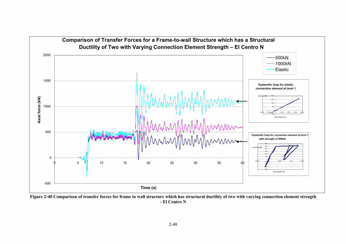
2�48

Figure 240 Comparison of transfer forces for frame to wall structure which has structural ductility of two with varying connection element strength

El Centro N

Comparison of Transfer Forces for a Frame�to�wall Structure which has a Structural

Ductility of Two with Varying Connection Element Strength – El Centro N

�500

0

500

1000

1500

2000

0 5 10 15 20 25 30 35 40

Time (s)

Ax

ial

forc

e (

kN

)

500kN

1000kN

Elastic

Hysteretic loop for connection element at level 1

with strength of 500kN

�400 �300 �200 �100

0 100 200 300 400 500 600

�0.0005 0 0.0005 0.001 0.0015

Axail elongation (m)

Axail force (kN)

Hysteretic loop for elastic

connection element at level 1

�500 0

500 1000 1500 2000

�0.0004 �0.0002 0 0.0002 0.0004 0.0006 0.0008

Axail elongation (m)

Axial force (kN)

2�49

2.3.6 Floor Diaphragm Stiffness

It was important to determine how sensitive the results were to the floor diaphragm thickness.

A sensitivity study was carried out on structures with floor diaphragm depths ranging between

0.25m to 0.4m thick which covers a realistic range of typical thicknesses that are used in

practice. The structures used were the 9�storey stiff and flexible structure with a fundamental

period of 0.58 and 1.44s. The parameters of these structures are provided in Section 2.3.4.

The floor diaphragms in this study represent floors which are relatively insensitive to flexural

deformations.

0 400 800 1200 1600 2000 2400

1

2

3

4

5

6

7

8

9

Transfer force (kN)

Le

ve

l

Comparison of Transfer Forces for Different Floor Diaphragm Thicknesses for the 9�Storey Stiff Structure �

El Centro N

0.4m

0.35m

0.30m

0.25m

Figure 2�41 Comparison of transfer forces for different floor diaphragm thicknesses for

the 9�storey stiff structure � El Centro N

2�50

0 500 1000 1500

1

2

3

4

5

6

7

8

9

Transfer force (kN)

Le

ve

l

Comparison of Transfer Forces for Different Floor Diaprhagm Thicknesses for the Flexible 9�Storey

Structure � El Centro N

0.4m

0.35m

0.3m

0.25m

Figure 2�42 Comparison of transfer forces for different floor diaphragm thicknesses for

the 9�storey flexible structure � El Centro N

Figure 2�41 and Figure 2�42 and provides comparisons between the magnitudes of floor

diaphragm link transfer forces for floor diaphragms of varying stiffness (thickness). These

figures indicate small variations in the trends and magnitudes of transfer forces for the range

of floor diaphragm thicknesses investigated. This indicates that significant variations in the

results should not be expected for different diaphragm thicknesses for floors which are

insensitivity to flexural deformations.

2.3.7 Structures of Different Heights

The influence of the height of the structure on the formation of floor diaphragm forces was

investigated. The heights of the structures included in the study were 3, 6, and 9 storey

buildings. The member sizes used in the 9 and 6�storey structure are the same as the member

sizes that were provided in Section 2.3.2. The member sizes that were used in the analytical

model for the 3�storey structure are provided in Table 2�9. Figure 2�43 indicates the

geometry of the structures used in the analysis.

2�51

Table 2�9 Member sizes used in the 3�storey analytical model

Stories SR Column Wall

3 1:0.3 0.85x0.85m 3.35x0.4m

1:1.14 0.64x0.64m 4.3x0.4m

6 1:0.61 1.1x1.1m 8.5x0.4m

1:1.49 0.95x0.95m 9x0.4m

1:2.63 0.85x0.85m 9.5x0.4m

1:3.51 0.7x0.7m 10x0.4m

6 storey 4 bay frame


Height =10.8m

Height =21.6m

Building details:

Storey height = 3.6m

Bay length=7m


Height =32.4m

Figure 2�43 Structures of varying heights

The structures investigated in this section have the same parameters as given in Section 2.2.3.

The structures were all designed for structural displacement ductility of 3. The fundamental

periods for the 3, 6 and the 9�storey structures were T1=0.275s, T1=0.321s and T1=0.567s

respectively.

The earthquake scale factors for the 3�storey and 6�storey structures are provided in Table

2�10. The earthquake scale factors for the 9�storey structure were provided in Section 2.3.

The New Zealand Structural Design Actions Standard NZS1170.5 (2004a) requires that when

the fundamental period for the structure is less than T1=0.4s the actual fundamental period

should not be used to scale the time history records and a period of 0.4s should be used

instead. For these cases, the scale factors were found by using a period of 0.4s.

2�52

Table 2�10 Scale factors for the earthquake records used in the analyses

Record Component k1 3�storey k1 6�storey

Lucerne North 0.92 1.01

Lucerne South 0.96 1.63

Izmit North 2.30 2.06

Izmit South 1.47 1.27

La Union North 2.13 1.98

La Union South 2.00 2.13

El Centro North 1.42 1.18

El Centro South 2.16 1.67

Llolleo North 0.95 0.89

Llolleo South 0.62 0.59

Tabas North 0.44 0.48

Tabas South 0.40 0.42

2.3.7.1 Total Floor Forces – 9 Storey

The following figures show the trends of average of the peak positive and negative total floor

diaphragm forces for structures with different heights for a selection of the structures that

were analysed. These figures show similar trends to the results from the other earthquake

records which are shown in Appendix A.3. The figures shown in this appendix provide

comparisons between total floor diaphragm forces for structures with different heights (3, 6

and 9 stories) and different structural ductilities.

0

1

2

3

4

5

6

7

8

9

10

2000 1000 0

Level

Force (kN)

Maximum Negative Force Envelope for

Different Stiffness Ratios with Structural

Ductility of 3 � El Centro N

SR 1:0.85

SR 1:1.23

SR 1:1.69

SR 1:2.58

0

1

2

3

4

5

6

7

8

9

10

0 1000 2000

Level

Force (kN)

Maximum Positive Force Envelope for

Different Stiffness Ratios with Structural


SR 1:0.85

SR 1:1.23

SR 1:1.69

SR 1:2.58

Figure 2�44 Maximum negative total force Figure 2�45 9� Maximum positive total

2�53

envelope for different stiffness ratios with

ductility of 3 � El Centro N

force envelope for different stiffness

ratios with ductility of 3 � El Centro N

0

1

2

3

4

5

6

7

8

9

10

4000 2000 0

Level

Force (kN)

Maximum Negative Force Envelope for Different Stiffness Ratios with Structural Ductility of 3 � Izmit N

SR 1:0.85

SR 1:1.23

SR 1:1.69

SR 1:2.58

0

1

2

3

4

5

6

7

8

9

10

0 2000 4000

Level

Force (kN)

Maximum Positive Force Envelope for Different Stiffness Ratios with Structural Ductility of 3 � Izmit N

SR 1:0.85

SR 1:1.23

SR 1:1.69

SR 1:2.58

Figure 2�46 Maximum negative total force


ductility of 3 � Izmit N

Figure 2�47 Maximum positive total force


ductility of 3 � Izmit N

0

1

2

3

4

5

6

7

8

9

10

6000 4000 2000 0

Level

Force (kN)

Maximum Negative Force Envelope for Different Stiffness Ratios with Structural

Ductility of 3 � Lucerne S

SR 1:0.85

SR 1:1.23

SR 1:1.69

SR 1:2.58

0

1

2

3

4

5

6

7

8

9

10

0 2000 4000 6000

Level

Force (kN)

Maximum Positive Force Envelope for Different Stiffness Ratios with Structural

Ductility of 3 � Lucerne S

SR 1:0.85

SR 1:1.123

SR 1:1.69

SR 1:2.58



ductility of 3 � Lucerne S



ductility of 3 � Lucerne S

2�54

0

1

2

3

4

5

6

7

8

9

10

4000 2000 0

Level

Force (kN)


Ductility of 3 � Tabas S

SR 1:0.85

SR 1:1.23

SR 1:1.69

SR 1:2.58

0

1

2

3

4

5

6

7

8

9

10

0 2000 4000

Level

Force (kN)



SR 1:0.85

SR 1:1.23

SR 1:1.69

SR 1:2.58



ductility of 3 � Tabas S



ductility of 3 � Tabas S

Figure 2�44 to Figure 2�51 show the maximum total floor force envelopes for the 9�storey

structure for different time history records. These figures provide information regarding how

the maximum total forces change for different levels in the structure.

The general magnitude of total forces over the height of the structure, observed from these

results, indicates that the total forces were variable at level 1 relative to the forces at the other

levels and the total forces were less at level 9 of the structure compared to the total forces at

the other levels. The variability in the total forces at level 1 is most likely due to the

variability in the inelastic deformation which develops in this level. The reason the forces

reduce at level 9 of the structures is due to the reason described in Section 2.3.1.

The distribution of the floor forces in the top levels of the structure for the Lucerne time

history records are slightly different to the values for the other earthquakes. Instead of a peak

occurring at level 8 a reduction occurs and a peak occurs at level 9 rather than a reduction

which is what is observed for the other earthquake records. The Lucerne record is a near fault

record which incorporates large directivity effects that applies a large pulse of energy to the

structure. The magnitudes of the scaled accelerations for the Lucerne and El Centro time

history records are shown in Figure 2�52.

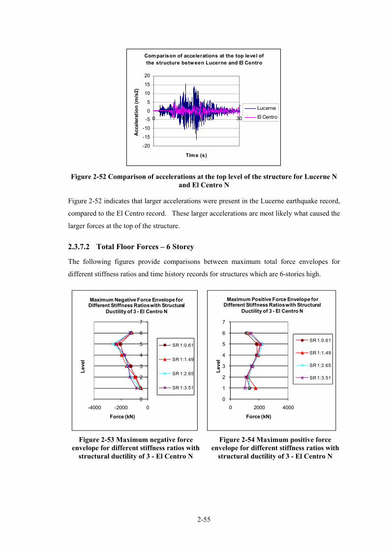
2�55

Comparison of accelerations at the top level of

the structure between Lucerne and El Centro

20

15

10

5

0

5

10

15

20

0 10 20 30

Time (s)

Accele

rati

on

(m

/s2)

Lucerne

El Centro

Figure 2�52 Comparison of accelerations at the top level of the structure for Lucerne N

and El Centro N

Figure 2�52 indicates that larger accelerations were present in the Lucerne earthquake record,

compared to the El Centro record. These larger accelerations are most likely what caused the

larger forces at the top of the structure.

2.3.7.2 Total Floor Forces – 6 Storey

The following figures provide comparisons between maximum total force envelopes for

different stiffness ratios and time history records for structures which are 6�stories high.

0

1

2

3

4

5

6

7

4000 2000 0

Level

Force (kN)



SR 1:0.61

SR 1:1.49

SR 1:2.65

SR 1:3.51

0

1

2

3

4

5

6

7

0 2000 4000

Level

Force (kN)



SR 1:0.61

SR 1:1.49

SR 1:2.65

SR 1:3.51

Figure 2�53 Maximum negative force


structural ductility of 3 � El Centro N

Figure 2�54 Maximum positive force



2�56

0

1

2

3

4

5

6

7

4000 2000 0

Level

Force (kN)

Maximum Negative Force Envelope for

Different Stiffness Ratios with

Structural Ductility of 3 � Izmit N

SR 1:0.61

SR 1:1.49

SR 1:2.63

SR 1:3.51

0

1

2

3

4

5

6

7

0 2000 4000

Level

Force (kN)

Maximum Positive Force Envelope for Different Stiffness Ratios with

Structural Ductility of 3 � Izmit N

SR 1:0.61

SR 1:1.49

SR 1:2.63

SR 1:3.51



structural ductility of 3 � Izmit N


envelope for different stiffness ratios

with structural ductility of 3 � Izmit N

0

1

2

3

4

5

6

7

10000 5000 0

Level

Force (kN)

Maximum Negative Force Envelope for Different Stiffness Ratios with

Structural Ductility of 3 � Lucerne S

SR 1:0.61

SR 1:1.49

SR 1:2.63

SR 1:3.51

0

1

2

3

4

5

6

7

0 5000 10000

Level

Force (kN)


Structural Ductility of 3 � Lucerne S

SR 1:0.61

SR 1:1.49

SR 1:2.63

SR 1:3.51



structural ductility of 3 � Lucerne S


envelope for different stiffness ratios

with structural ductility of 3 � Lucerne S

2�57

0

1

2

3

4

5

6

7

4000 2000 0

Level

Force (kN)



SR 1:0.61

SR 1:1.49

SR 1:2.63

SR 1:3.51

0

1

2

3

4

5

6

7

0 2000 4000

Level

Force (kN)



SR 1:0.61

SR 1:1.49

SR 1:2.63

SR 1:3.51



structural ductility of 3 � Tabas S



structural ductility of 3 � Tabas S

The distribution of floor forces for the 6�storey structure shown in Figure 2�53 to Figure 2�60

are similar to the trends for the 9�storey structures. The variations of the total forces with

height of the structure are much less compared to those variations for the 9�storey structures.

This is because higher modes are not as significant for shorter structures. The similarities

between the total floor force distribution for the 6 and 9�storey structures indicate the

possibility of developing a static type method to approximate the forces in the floor

diaphragm. These figures also illustrate that different trends developed for the force

envelopes at the top of the structure when subjected to Lucerne time history record.

2�58

2.3.7.3 Total Floor Forces 3�Storey

0

1

2

3

4

4000 2000 0

Level

Force (kN)

Maximum Negative Force Envelope for Different Stiffness Ratios with

Structural Ductility of 3 � El Centro N

SR 1:0.30

SR 1:1.14

0

1

2

3

4

0 2000 4000

Level

Force (kN)


Structural Ductility of 3 � El Centro N

SR 1:0.30

SR 1:1.14




Figure 2�62 Maximum positive total

force envelope for different stiffness

ratios with structural ductility of 3 –

El Centro N

Figure 2�61 and Figure 2�62 show the typical maximum total force envelopes for a 3�storey

structure for all time history records. These figures show a decrease of total force for the

floor at level 3 of the structure which is similar to the findings for the taller structures. Also

similar to the taller structures, different trends are shown for the results from the near field

record of Lucerne.

The inertial floor forces for these structures are generally found to increase with the height of

the structure as shown in Figure 2�63 to Figure 2�64.

0

1

2

3

4

2000 0 2000 4000

Level

Force (kN)

Maximum Positive Combination of Transfer and Inertial Forces for SR

1:0.30 with Structural Ductility of 3 �El Centro N

Transfer

Inertia

Total

0

1

2

3

4

2000 0 2000 4000

Level

Force (kN)


1:1.14 with Structural Ductility of 3 �El Centro N

Transfer

Inertia

Total

Figure 2�63 Maximum positive

combination of transfer and inertial forces

for SR 1:0.3 with structural ductility of 3 –

El Centro N



for SR 1:1.14 with structural ductility of 3

� El Centro N

2�59

Figure 2�63 and Figure 2�64 indicate that transfer forces are less than inertial forces,

especially at levels 1 and 3. The small transfer forces which have been observed to develop at

level 1 of the structure are not similar to the results of the 6 and 9�storey structures. The

reason that transfer forces are smaller for this height of structure is because the wall and the

frame elements are not tall enough to form large deformation patterns and therefore resist

each other. The transfer forces here are not negligible though; they still increase the level of

total force noticeably as shown in the figures above and therefore should still be considered

for shorter structures.

2.3.8 Total Forces in Low Seismic Zones

For this research, the magnitude of total floor forces and the components of the total forces,

inertia and transfer forces, in the floor diaphragm link element were investigated for low

seismic zones. This study was carried out to determine the importance of considering transfer

forces in structures that are typically constructed in these zones.

Auckland is a reasonably low seismic region in New Zealand; the design response spectra

from NZS1170.5 (2004a) for this region will be used to scale various time history records for

the analyses. The analytical model that was used for this analysis was similar to the model

described above but it was adjusted for strength and stiffness to represent typical Auckland

structures.

Frame�to�wall dual structures in low seismic regions generally result in the frame hanging off

the wall structure as the frame is typically relatively flexible to the wall elements. It has been

shown previously for a structure with very flexible element and a stiff element, only small

transfer forces develop and the structure will deform predominantly like the stiff element in

this case the walls, typically. The structure for this investigation was developed to represent

the case where transfer forces would be the largest. From previous sections of this study it

was found that a structure with similar stiffness between the frame and wall elements and a

structure which is reasonably tall, in general, results in larger transfer forces.

The structure used for this study was a 9�storey structure with a frame�to�wall stiffness ratio

of 1:0.7; this consisted of columns of 0.60m by 0.60m, a wall of 2m by 0.2m, 0.6m by 0.4m

beams and 3.6m inter�storey height. The fundamental translational period of the structure was

T1 = 1.435s which is comparable to the fundamental periods of Tremayne and Kellys’ work

(2005).

2�60

The time history records used to represent the Auckland region were suggested by the

Institute of Geological and Nuclear Sciences (GeoNet, 2008). The records used were the

North and South components of; El Centro, Delta, Kalamata, Karinthos, Matahina and

Bovino. A description of these earthquake records is provided in Table 2�11.

Table 2�11 Low seismicity earthquake records

Ref Name Location Date Magnitude

1 El Centro USA, El Centro, Imperial

Valley

19 May 1940 7.0

2 Delta USA, Mexico, Delta,

Imperial Valley

15 October

1979

6.5

3 Kalamata Greece, Kalamata 13 September

1986

5.8

4 Karinthos Greece, Karinthos, Alkion 24 February

1981

6.7

5 Matahina Edgecumbe Earthquake,

Matahina Dam

2 March 1987 6.5

6 Bovino Italy, Bovino, 23 November

1980

6.8

These records have been scaled for the Auckland region with a soil structure of shallow soil

representing the sedimentary rocks in the Ponsonby area, for example (Kermonde, 1992).

The earthquake scale factors used for this analysis are provided in Table 2�12. The gaps

shown in this table represent records which were discarded by the limitations in the scaling

procedure presented in the New Zealand Loadings Standard (Standards New Zealand, 2004a).

Table 2�12 Scale factors for the earthquake records used in the analyses

Record Component k1 9storey

El Centro North 0.36

El Centro South 0.45

Delta North �

Delta South 0.45

Kalamata North 0.47

Kalamata South 0.51

Karinthos North 0.46

Karinthos South 0.58

Matahina North 0.58

Matahina South 0.61

Bovino North �

Bovino South �

2�61

As for the previous time history record scaling only the k1 factor has been used here. The k2

factor has been discarded as it introduces unnecessary conservatism in the results.


The following figures show the maximum total floor force envelopes for the range of time

history records for the Auckland structures.

0

1

2

3

4

5

6

7

8

9

10

800 600 400 200 0

Level

Force (kN)

Maximum Negative Force Envelopes for Different Time History Records with

Structural Ductility of 3

El Centro 1

El Centro 2

Delta 2

Kalamata 1

Kalamata 2

Karinthos1

Karinthos 2

Matahina 1

Matahina 2

0

1

2

3

4

5

6

7

8

9

10

0 200 400 600 800

Le

vel

Force (kN)

Maximum Positive Force Envelopes for Different Time History Records with

Structural Ductility of 3

El Centro 1

El Centro 2

Delta 2

Kalamata 1

Kalamata 2

Karinthos1

Karinthos 2

Matahina 1

Matahina 2


envelopes for different time history records

with structural ductility of 3


envelopes for different time history

records with structural ductility of 3

Figure 2�65 and Figure 2�66 show the maximum total force envelopes for the Auckland

structures. These figures indicate a general trend of increasing total force with increasing

height of the structure. Both of the total force envelopes show a reduction of magnitude

around levels 6 and 7 of the structure. The components of transfer and inertial which make up

the total force envelopes were investigated. Figures showing this comparison are provided

below.

2�62

200 0 200 400 600

1

3

5

7

9

Force (kN)

Level

Comparison of the transfer and

inertia components that give the

maximum envelope for El Centro N

Transfer

Inertia

200 0 200 400 600

1

3

5

7

9

Force (kN)

Level

Comparison of the transfer and inertia components that give the

maximum envelope for El Centro S

Transfer

Inertia

Figure 2�67 Comparison of the transfer

and inertia components that give the

maximum envelope for El Centro N



maximum envelope for El Centro S

200 0 200 400 600

1

3

5

7

9

Force (kN)

Level

Comparison of the transfer and

inertia components that give the

maximum envelope for Delta S

Transfer

Inertia

200 0 200 400 600

1

3

5

7

9

Force (kN)

Level

Comparison of the transfer and inertia

components that give the maximum envelope for Kalamata N

Transfer

Inertia



maximum envelope for Delta S



maximum envelope for Kalamata N

Figure 2�67 to Figure 2�70 show that the magnitudes of transfer forces are negligible

compared to the inertial forces for these structures designed for a low seismic region. The

reason the magnitudes of transfer forces are less for this structure is due to the flexible nature

of both the wall and the frame components of the structure. The high flexibility of these

elements allows each element to conform to a similar deformation pattern much easier than

stiff elements would. This research indicates that for flexible structures, designed for low

seismic regions, transfer forces are significantly less than for stiff structures in high seismic

regions.

2�63

2.3.9 Tower�to�Podium Structures

As discussed in the introduction to transfer forces, a variety of structures exist, other than

frame�to�wall structures, where transfer forces are likely to be significant. Tower to podium

structures are examples of this. Transfer forces are likely to be important in these structures

due to the variation of the vertical stiffness of the lateral force resisting elements. An

example of this type of structure is provided in Figure 2�71.

Figure 2�71 New Zealand Post Building, Wellington

Section 2.2.2 provides a description of the general layout of the structural system used in the

analytical model. The layout of this set of structures was based on the original 9�storey

frame�to�wall structure with a fundamental period of T1=0.58s which was used in Section

2.2.3. This set of structures is the stiffest of the group of structures 9�storey structures

analysed so far (T1=0.58s, T1=0.97s and T1=1.44s). The structure with the largest global

stiffness has been chosen as when the wall terminates the change in stiffness will be larger

than for the other more flexible structures. This therefore presents the worst case. Two

different frame�wall stiffness ratios for each type of podium structure were investigated; these

were SR1:4.9and SR 1:9.9 for the 3�storey podium and SR1:1.8 and SR1:3.3 for the 6�storey

podium structure. These stiffness ratios are from comparing the stiffness of the individual

frame and wall elements at the top of the podium. These values were selected as they cover

the range of stiffness ratios used in previous sections of this research. This allowed

comparisons to be made with previous results and also allowed investigations to be made on

the effect of varying frame�to�wall stiffness ratios in this type of structure.

2�64

It has been found by previous work that the two structural displacement ductility levels

(ductility of two and three) both produce large magnitudes of total diaphragm forces. A

pushover analysis was carried out to determine the ductility level of these structures. As the

structure is not a regular structure, three different loading shape functions were used in the

pushover analyses; these were the ESA load pattern from the New Zealand Structural Design

Action Standards (Standards New Zealand, 2004a), pESA method mentioned earlier in this

report and a constant load pattern with height. The force displacement plots from the

pushover analysis were found to be similar for each of these loading profiles. From these

results the structural ductility level for this group of structures was found to be around three.

The fundamental periods of the structures with differing frame�to�wall SRs was allowed to

vary slightly. In other sections of this research the fundamental periods have been kept

similar, here they have not as the structural system has been changed. The fundamental

translational period, T1, for the 3�storey structures of different stiffness ratios were found to

vary, the period for the 6�storey structures remained reasonably constant. This occurred

because the frame is the predominant part of the structure (9�stories) in relation to the wall (3�

stories). Therefore the period changes as the sizes of the columns in each of the frames are

different due to the different frame�to�wall stiffness ratios.

Table 2�13 Fundamental periods for each of the structures

SR 1:1.8 SR 1:3.3

6�storey wall 0.53s 0.53s

SR 1:4.4 SR 1:9.9

3�storey wall 0.59s 0.68s

To ensure reasonable trends were identified from the results, twelve time history records

which represent the Wellington region were used in this investigation. A description of these

records and how these records are scaled are described in Section 2.2.6.

2�65

Table 2�14 Scale factors for the earthquake records for the podium structure models

k1 3�storey wall k1 6�storey wall

Record Comp. SR 1:4.4 SR 1:9.9 SR 1:1.8 SR 1:3.3

Lucerne North 0.99 1.02 1.06 1.06

Lucerne South 1.39 1.44 1.39 1.39

Izmit North 1.88 1.93 1.88 1.82

Izmit South 1.59 1.65 1.56 1.56

La Union North 1.65 1.58 1.75 1.75

La Union South 1.98 2.05 2.00 2.00

El Centro North 0.95 0.91 0.97 0.97

El Centro South 1.38 1.32 1.42 1.42

Llolleo North 0.80 0.78 0.82 0.82

Llolleo South 0.55 0.54 0.55 0.55

Tabas North 0.47 0.46 0.50 0.50

Tabas South 0.40 0.41 0.42 0.42

2.3.9.1 Floor Forces for the 3�Storey Wall 9�Storey Frame Structure

A selection of the figures which present the total floor diaphragm forces obtained from the

time history analysis for the 3�storey wall podium structures are provided below. The results

shown in these figures are similar to the results obtained from other time history records that

were included in the study. These figures are provided in Appendix A.5.1.1.

0

1

2

3

4

5

6

7

8

9

10

0 2500 5000

Level

Force (kN)

Maximum Total Force Envelope for Different Stiffness Ratios with Structural


SR 1:4.9

SR 1:9.9

0

1

2

3

4

5

6

7

8

9

10

0 2500 5000

Level

Force (kN)


Ductility of 3 � Lucerne N

SR 1:4.9

SR 1:9.9

Figure 2�72 Maximum total force

envelopes for different stiffness ratios with

structural ductility of 3 – El Centro N



structural ductility of 3– Lucerne N

2�66

0

1

2

3

4

5

6

7

8

9

10

0 2500 5000

Lev

el

Force (kN)


Ductility of 3 � Izmit N

SR 1:4.9

SR 1:9.9

0

1

2

3

4

5

6

7

8

9

10

0 2500 5000

Level

Force (kN)


Ductility of 3 �La Union N

SR 1:4.9

SR 1:9.9



structural ductility of 3 – Izmit N



structural ductility of 3 – La Union N

Figure 2�72 to Figure 2�75 provides a comparison of the maximum total force envelopes for

the floor diaphragms for structure with different stiffness ratios and different time history

records. These figures show similar trends. A large increase in total force for the diaphragms

was found to develop at level 3 of the structure compared to the other levels in the structure.

This is due to the large change in vertical stiffness which occurs at this level. These results

indicate that floor diaphragms at the podium�to�tower interface need special attention in the

design process. To verify that the large force at this interface is due to transfer forces the

components of force have been looked at in the following figures.

0

1

2

3

4

5

6

7

8

9

10

0 2500 5000

Le

vel

Force (kN)

Maximum Total Force Component Envelopes for SR1:4.9 with Structural


Transfer

Inertia

Total

0

1

2

3

4

5

6

7

8

9

10

0 2500 5000

Lev

el

Force (kN)

Maximum total Force Component Envelopes for SR1:9.9 with Structural


Transfer

Inertia

Total

Figure 2�76 Maximum force component

envelopes for SR1:4.9 with structural

ductility of 3 – La Union N

Figure 2�77 Maximum force component

envelopes for SR1:9.9 with structural

ductility of 3 – La Union N

2�67

Figure 2�76 to Figure 2�77 show the maximum force component envelopes for the floor

diaphragm for each of the stiffness ratios. It should be noted that the transfer forces are zero

above level 3 as this is where the wall finishes. These figures show the large forces at level 3

of the 3�storey wall podium structure are due to transfer forces and not inertial forces. All of

these figures show that at level 3 the magnitudes of transfer forces are many times large than

inertial forces.

2.3.9.2 Floor Forces for the 6�Storey Wall 9�Storey Frame Structure

A selection of the total floor force results for the 6�storey wall 9�storey frame structures from

some of the time history records are shown in the following figures. These figures are

generally representative of all the results from the different time history records that were

included in this study. The results from the different time history records are provided in

Appendix A.5.1.2.

0

1

2

3

4

5

6

7

8

9

10

0 2000 4000

Level

Force (kN)



SR 1:1.8

SR 1:3.3

0

1

2

3

4

5

6

7

8

9

10

0 2000 4000

Level

Force (kN)



SR 1:1.8

SR 1:3.3



structural ductility of 3 – El Centro N



structural ductility of 3 – Izmit N

2�68

0

1

2

3

4

5

6

7

8

9

10

0 2000 4000

Level

Force (kN)



SR 1:1.8

SR 1:3.3

0

1

2

3

4

5

6

7

8

9

10

0 2000 4000

Level

Force (kN)


Ductility of 3 �Llolleo N

SR 1:1.8

SR 1:3.3



structural ductility of 3 – La Union N



structural ductility of 3 – Llolloe N

Figure 2�78 to Figure 2�81 indicates different results to those of the 3�storey wall 9�storey

frame podium structure. The 6�storey wall podium structure results seem to be a combination

of the typical full height 9�storey frame�to�wall structure results and the results of the 3�storey

wall podium structure. Large transfer forces are observed at level 1 of the structure; this is

typical of the non�podium structure with the full height wall. This trend was not so obvious

for the 3�storey wall structure as a result of the large transfer forces which developed at

level 3. For the 6�storey wall podium structure the total forces then increase up to level 5 and

then decrease over level 6 and 7. The increase of forces in the vicinity of terminated wall is

similar, but not as severe as the large forces observed at level 3 of the 3�storey podium

structure.

To determine the relative contribution of inertia and transfer forces the components total force

for these structure was plotted in the following figures.

2�69

0

1

2

3

4

5

6

7

8

9

10

0 2000 4000

Le

vel

Force (kN)

Maximum Total Force Envelope Components for SR 1:1.8 with Structural


Transfer

Inertia

Total

0

1

2

3

4

5

6

7

8

9

10

0 2000 4000

Le

vel

Force (kN)

Maximum total Force Envelope Components for SR 1:3.3 with Structural


Transfer

Inertia

Total

Figure 2�82 Maximum total force envelope

components for SR1:1.8 with structural

ductility of 3 – Izmit N

Figure 2�83 Maximum total force envelope

components for SR1:3.3 with structural

ductility of 3 – Izmit N

Figure 2�82 to Figure 2�83 show that transfer forces generally provide the largest contribution

to the total forces at level 1 of the structure. These figures show for level 6 of the structure

with the stiffness ratio of SR1:8 the magnitude of inertial and transfer forces were similar and

for SR 1:43 and SR 1:233 the magnitude of transfer forces was larger than inertial forces.

This result was typical for half of the time history records. For the other time history records,

the magnitude of transfer and inertial forces were found to be similar at level 6 of the

structure for all of the stiffness ratios.

The difference in the magnitude of transfer forces between the 3 and the 6�storey podium�to�

wall structures is due to the relative change in vertical stiffness. For the 3�storey wall

structure the change in vertical stiffness is much greater than for the 6�storey wall structure.

Typically a wall element is stiffest at the lower levels and more flexible at the upper levels

whereas a frame element is more flexible at the lower levels and relatively stiffer at the upper

levels. For the 3�storey wall structure the wall is terminated at a level where it provides large

stiffness contribution and the frame contributes little stiffness. Further, for the 6�storey wall

structure the wall is terminated when the wall is becoming flexible and the frame is becoming

stiff; therefore the relative change in stiffness is less abrupt than the 3�storey wall structure.

2.3.10 Structures with Different Length Walls

Research carried out by Rutenberg and Leibovich (2002), Beyer (2005) and Priestley et

al.(2007), which is described in the literature review in Section 2.1, suggested that walls of

different lengths typically deform differently. Beyer (2005) carried out an extensive study on

2�70

the design and analysis of walls of different length and also the sensitivity of transfer forces in

the floor diaphragm. Investigations are carried out, which focus on transfer forces in walls of

different lengths, to complete this study and also tie in with the research carried out by Beyer.

Figure 2�84 Walls of different length analytical model

The trends of transfer forces were investigated for these structures. Figure 2�84 provides a

graphical representation of the model that will be analysed in this section. Nine different

wall�to�wall stiffness ratios will be investigated using 12 earthquake records that represented

the seismicity in the Wellington region (Section 2.2.6). The stiffness ratios were calculated

by carrying out pushover analyses for the individual walls. The fundamental periods for each

structure were kept constant to allow comparisons between structures with similar dynamic

flexibilities. The period for these structures was T1 = 0.482s. This value is slightly less than

the 9�storey frame�to�wall structure with a period of T1=0.576s. Wall�to�wall structures are

inherently stiffer than frame�to�wall structures therefore a shorter fundamental period is

expected. The lengths of walls in this study vary between 1m and 13m long. The stiffness

ratios and wall lengths used in the analyses are provided in Table 2�15.

2�71

Table 2�15 Different wall lengths and stiffness ratios

Wall A

(m)

Wall B

(m)

Stiffness

Ratio

1 12.65 1:232

2 12.85 1:107

3 12.95 1:45

4 13.05 1:24

5 13.00 1:14

6 12.95 1:9

7 12.85 1:6

8 12.60 1:4

9 12.20 1:2

Structures of 9�stories high were investigated for this study as it was identified in previous

studies that taller structures provide larger transfer forces. Plastic hinges have been designed

to develop at the base of each of the walls. Lumped plasticity was used in the model; the

effects of this assumption were investigated in Chapter 3. Shear deformations were ignored

in this initial study, the effect of this assumption is considered in the sensitivity study

provided in Chapter 3. The time history records for the Wellington region were used in this

study. The time history records were scaled as described in Section 2.2.6. The scale factors

are provided in Table 2�16 below.

Table 2�16 Time history scale factors

Record k1

Lucerne N 1.06

Lucerne S 1.31

Izmit N 1.88

Izmit S 1.59

La Union N 1.86

La Union S 2.03

El Centro N 1.05

El Centro S 1.50

Llolleo N 0.88

Llolleo S 0.56

Tabas N 0.48

Tabas S 0.40

2�72

2.3.10.1 Total Floor Force

Figures showing some of the total, inertial and transfer force results in the floor diaphragms

for the wall�to�wall structures are shown below.

0

1

2

3

4

5

6

7

8

9

10

3000 2000 1000 0

Le

ve

l

Force (kN)

Maximum Negative Total Force Envelope for Different Stiffness

Ratios � El Centro N

SR 1:232

SR 1:107

SR 1:45

SR 1:24

SR 1:14

SR 1:9

SR 1:6

SR 1:4

SR 1:2

0

1

2

3

4

5

6

7

8

9

10

0 1000 2000 3000

Level

Force (kN)

Maximum Positive Total Force Envelope for Different Stiffness

Ratios � El Centro N

SR 1:232

SR 1:107

SR 1:45

SR 1:24

SR 1:14

SR 1:9

SR 1:6

SR 1:4

SR 1:2


envelopes for different stiffness ratios �

El Centro N


envelopes for different stiffness ratios �

El Centro N

Figure 2�85 and Figure 2�86 show the total floor force envelope for the wall�to�wall structures

in response to El Centro earthquake excitation. These results are typical of the results from

the other time history records which are presented in Appendix A.6. This appendix provides

total floor diaphragm forces and components of total floor diaphragm forces for structures

with walls of different lengths. These figures generally show an increase of forces with

height up the structure. This is expected due to the increase of accelerations and hence

inertial forces which occur with height. For some of the results large total forces were

observed at level 1 of the structure. Large forces develop because walls are stiffest at the

lower levels and the most inelastic deformations occur at the lower levels. The research

carried out by Beyer indicated that walls are better modelled with distributed plasticity

compared to lumped plasticity. The sensitivity affects of using a lumped plasticity model is

considered in Chapter 3.

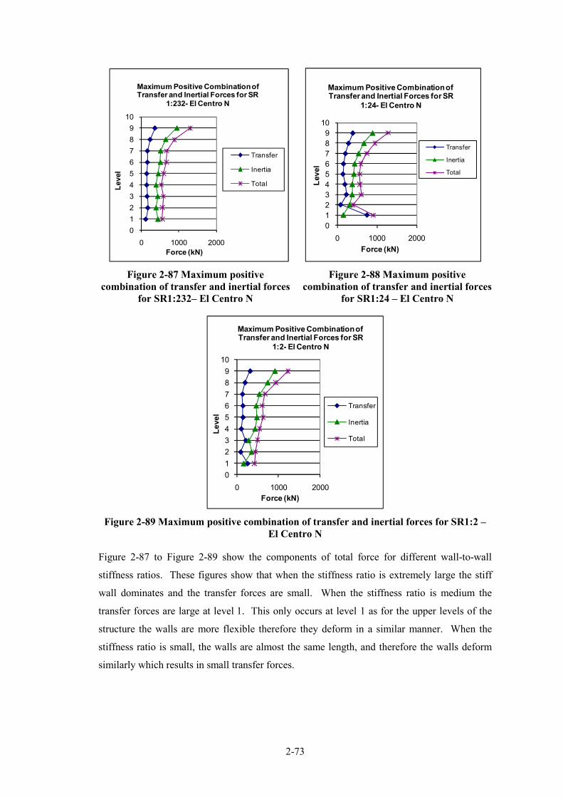
2�73

0

1

2

3

4

5

6

7

8

9

10

0 1000 2000

Level

Force (kN)


1:232� El Centro N

Transfer

Inertia

Total

0

1

2

3

4

5

6

7

8

9

10

0 1000 2000

Level

Force (kN)


1:24� El Centro N

Transfer

Inertia

Total



for SR1:232– El Centro N



for SR1:24 – El Centro N

0

1

2

3

4

5

6

7

8

9

10

0 1000 2000

Level

Force (kN)


1:2� El Centro N

Transfer

Inertia

Total

Figure 2�89 Maximum positive combination of transfer and inertial forces for SR1:2 –

El Centro N

Figure 2�87 to Figure 2�89 show the components of total force for different wall�to�wall

stiffness ratios. These figures show that when the stiffness ratio is extremely large the stiff

wall dominates and the transfer forces are small. When the stiffness ratio is medium the

transfer forces are large at level 1. This only occurs at level 1 as for the upper levels of the

structure the walls are more flexible therefore they deform in a similar manner. When the

stiffness ratio is small, the walls are almost the same length, and therefore the walls deform

similarly which results in small transfer forces.

2�74

2.3.11 Can Inertia and Transfer Forces be Treated Separately?

As described in Section 2.1.2, traditionally transfer and inertial forces have been treated

separately. However, theoretically, these forces should be treated simultaneously. An

investigation on the effect of treating these forces separately is carried out in this section.

The total floor force envelope where the combination of inertial and transfer force was

maximum, over the height of the structure, is compared to the combination of the maximum

inertial forces plus the maximum transfer forces.

0

2

4

6

8

10

0 1000 2000 3000

Le

vel

Force (kN)

Comparison between Maximum Total

forces and combination of maximum Inertia and Transfer Force SR 1:0.85 �

El Centro N

Approximate

envelope

Actual

Envelope

0

2

4

6

8

10

0 1000 2000

Level

Force (kN)

Comparison between Maximum Total forces and combination of maximum

Inertia and Transfer Force R 1:2.58 �La Union N

Approximate

envelope

Actual

Envelope

Figure 2�90 Comparison between

maximum total forces and combination of

maximum inertia and transfer forces

SR1:0.85 – El Centro N

Figure 2�91 Comparison between

maximum total forces and combination of

maximum inertia and transfer forces SR

1:2.58 – La Union N

Figure 2�90 and Figure 2�91 provide comparisons between the maximum envelope of the

components of inertia and transfer force summed together separately (approximate envelope)

and the maximum actual total force envelope from the maximum combination of inertial and

transfer forces from actual time step (actual envelope). These figures suggest that taking the

maximum inertial and maximum transfer forces and independently adding them together

provides reasonable results for the middle levels of the structure, but poor results for the top

and bottom levels of the structure. The poor results for the top and bottom levels of the

structure indicate that maximum inertial and transfer forces at these levels occur at different

times. By using independent transfer and inertial forces this phenomenon is not identified.

This indicates that both transfer and inertia forces need to be determined simultaneously by

considering both forces with respect to time of occurrence.

2�75

2.4 Conclusions

The following bullet points provide a summary of the findings of the above described

investigations on the forces which develop in floor diaphragms:

− Large transfer forces with the floors, acting as diaphragms, have been found to

develop in structures where the relative stiffness of the vertical elements such as

frame and wall elements are of similar magnitudes and the structure is of a

reasonable height (greater than 3�stories). This occurs as both elements are stiff

enough to resist the desired deformation pattern of the other element;

− In structures where the stiffness contribution of the frame and the wall elements are

different, where one element is very stiff and the other is very flexible, the flexible

element goes ‘along for the ride’ and provides little resistance to the deformations

imposed by the stiffer element. This results in smaller transfer forces developing

within the floor diaphragm;

− The magnitudes of the transfer forces are found to change direction (sign) compared

to inertial forces for the upper level of the frame�to�wall structures. This is due to

the different deformation patterns for these elements; at the lower levels of the

structure the wall will pull the frame and at the upper levels the frame will pull the

wall;

− Inelastic deformation of a structure results in permanent lateral deformations, which

is the cause of residual forces in floors;

− Inelastic action in the diaphragm between the wall and the frame element is found to

reduce the residual transfer forces but may not completely remove them;

− Elastic analysis has been found to poorly predict transfer force results and is not

recommended for any type of analysis where transfer forces maybe significant.

Also elastic analysis of these structures does not identify the development of

residual transfer forces in the structure;

− General trends of the distributions of floor forces were found to be reasonably

consistent for dual structures of different heights. The magnitudes of these forces

were found to vary as a result of different flexibilities of the vertical lateral force

resisting elements within the structures;

− Transfer forces are found to be small for low seismic regions such as Auckland due

to the typical flexibility of structures in these zones;

− Large transfer forces were found to occur for podium structures. These large forces

occurred at the interface of the podium and the tower. It was found that the transfer

forces were less when the podium of the structure was located higher up the

structure;

2�76

− Transfer forces were found to develop in structures with walls of different length.

These forces predominantly formed at the bottom of the structure where the

deformation patterns differ. The magnitude of transfer forces was found to reduce

with increasing height of the walls as the flexibility of the wall increased;

− It was found that if inertia and transfer forces were treated separately, poor

predictions were obtained for the total force in the upper and lower levels of the

structure and reasonable comparisons were found for the middle levels of the

structure. This indicates that maximum inertia and transfer forces occur at similar

times in the middle levels of the structure but not at the upper and lower levels.

2.5 References

ACI Committee 318. (2008). Building Code Requirements for Structural Concrete (ACI318�

08) and Commentary. American Concrete Insitute.

Begg, J. G. and Mazengarb, C. (1996). Geology of the Wellington Area. Lower Hutt, New

Zealand, Institute of Geological & Nuclear Sciences Limited.

Bentz E. C., a. C. M. P. (2002). Response, Reinforce Sectional Analysis using Modificed

Compression Field Theory.

Bentz, E. C. and Collins, M. P. (2002). Response, Reinforce Sectional Analysis using

Modificed Compression Field Theory.

Berberian, M. (1978). "Tabas�e�Golshan (Iran) Catastrophic Earthquake of 16 September

1978: A Preliminary Field Report." Disasters Volume 2( 4): 207�219.

Beyer, K. (2005). Design and Analysis of Walls Coupled by Floor Diaphragms. European

school of advanced studies in reduction of seismic risk. Pavia, ROSE School. Master

Degree: 118.


Technical Report No. 20, New Zealand Concrete Society. Technical Report No. 20: .

Bull, D. K. (2003). "Understanding the Complexities of Designing Diaphragms in Buildings

for Earthquakes." Bulletin of the New Zealand National Soicety for Earthquake

Engineering 37(2).

2�77

Carr, A. J. (1981�2009b). Ruaumoko Computer Program Library Volume 2: User Manual for

the 2�Dimensional Version Ruaumoko 2D. Christchurch, New Zealand, University of

Canterbury.

Carr, A. J. (1981�2009c). Ruaumoko Computer Program Library Volume 3: User Manual for


Canterbury.

Carr, A. J. (1981�2009d). Ruaumoko Computer Program Library Christchurch, New Zealand,

University of Canterbury.

Carr, A. J. (1997). Damping Models for Inelastic Analyses. Asia�Pacific Vibration

Conference, Kyongju, Korea.

Clendon, J. E. (1985). Alternative Damping Models Civil Engineering. Christchurch, New

Zealand, University of Canterbury. Master of Engineering 65.

Clough, D. P. (1982). "Considerations in the Design and Construction of Precast Concrete

Diaphragms for Earthquake Loads." Journal Prestressed Concrete Institute 27(2): 78�

93.

Fleischman, R. B. and Farrow, K. T. (2002). "Dynamic Behavior of Perimeter Lateral�system

Structures with Flexible Diaphragms." Earthquake Spectra 18(2): 251�286.

Fleischman, R. B., et al. (2004). "Development of a Seismic Design Methodology for Precast

Diaphragms Part 1: Design Framework." PCI Journal 50(5): 68�83.

Flores Ruiz, J. A. (2005). Performance of Ductile Reinforced Concrete Moment Resisting

Frames Subject to Earthquake Actions. Civil Engineering. Christchurch, New Zeland,

University of Canterbury. Master of Engineering: 233.

GeoNet (2008). Strong Motion Database, Geological Nueclear Science and Earthquake

Commision.

Goodsir, W. J. (1982). The Inelastic Seismic Response of Reinforced ConcreteFrame Shear�

wall Structures. Christchurch, N.Z., Department of Civil Engineering University of

Canterbury: 155.

Kelly, T. (2004). "Nonlinear Analysis of Reinforced Concrete Shear Wall Structures."

Bulletin of the New Zealand National Society for Earthquake Engineering 37(4): 156�

180.

2�78

Kermonde, L. (1992). Geology of the Auckland Urban Area. Lower Hutt, New Zealand,

Institute of Geological & Nuclear Sciences Limited.

McVerry, G. (2003). Accelerograms Selected as Rock Records for Wellington City, Institute

of Geological and Neclear Sciences.

Muto, K. (1974). A Seismic Design Anaysis of Buildings. Maruzen, Tokyo.

Paulay, T. and Priestley, M. J. N. (1992). Seismic Design of Reinforced Concrete and

Masonry Buildings. New York, N.Y., Wiley.




Priestley, M. J. N., et al. (2007). Displacement�Based Seismic Design of Structures. Pavia,

Italy, IUSS Press.

Priestley, M. J. N. and Grant, D. N. (2005). "Viscous Daming in Seismic Design and

Analysis." Journal of Earthquake Engineering 9(2): 229�255.

Rathje, E., et al. (2000). "Strong Ground Motions and Site Effects." Earthquake Spectra 16(n

SUPPL. A): 65�96.

Reyners, M., et al. (1999). "A Three�Dimensional Image of Shallow Subduction: Crustal

Structure of the Raukumara Peninsula, New Zealand." Geophysical Journal

International 137: 873�890.



Rutenberg, A. and Leibovich, E. (2002). "On the Lateral Force Distribution Among Structural

Walls in Multistorey Buildings." Bulletin of the New Zealand National Soicety for

Earthquake Engineering 35(4): 231�242.

Somerville, P. G., et al. (1997). "Modification of Emperical Strong Ground Motion

Attenuation Relations to Include the Amplitude and Duration Effects of Rupture

Directivity." Seismological research letters, Seismological Society of America.

Eastern Section., Vol. 68(1): 199�222.

2�79

Standards New Zealand (2004a). Structural Design Actions Part 5. Wellington, Standards

New Zealand.



Standards New Zealand. (2004). Structural design actions part 5. Wellington [N.Z.],


Stewart, J. P., et al. (1999). "Seismic Soil�Structure Interaction in Buildings: Analytical

Methods." Journal of Geotechnical and geoenvironmental engineering 125(1): 26�37.

Stewart, N. L. (1995). An Analytical Study of the Seismic Response of Reinforced Concrete

Frame�Shear Wall Structures Civil Engineering. Christchurch, New Zealand,

University of Canterbury. Master of Engineering: 126.

Sullivan, T. J., et al. (2006). Seismic Design of Frame�Wall Structures. Pavia, Italy, IUSS

Press.

Takeda, T., et al. (1970). "Reinforced Concrete Response to Simulated Earthquakes."

Tremayne, B. and Kelly, T. (2005). Time History Analysis as a Method of Implementing

Performanced Based Design. New Zealand National Soicety for Earthquake

Engineering. Taupo, New Zealand.

University of California (2005, 2007). "Pacific Earthquake Engineering Strong Motion

Database: NGA."

2�80

3�1

3 SENSITIVITY STUDY: MODELLING FLOOR

DIAPHRAGM FORCES

Sensitivity analyses were carried out on the modelling assumptions that were made for the

floor force analytical models described in Chapter 2 of this report. This was carried out to

determine the importance of each modelling assumption by determining how these affected

the results. It was anticipated that an importance hierarchy of the modelling parameters could

be developed.

3.1 Foundation Flexibility

The sensitivity of the rigid foundation assumption was investigated. It was thought that this

assumption would have a reasonable affect on the forces which develop in the floor

diaphragms as additional flexibility from the foundation would affect the deformations of the

structure. A variety of literature has also indicated that foundation flexibility effects should

be considered when modelling any type of structure. This section describes how foundation

flexibility affects the magnitudes of total floor forces which develop in a variety of different

structures. Foundation models of different complexity were analysed to determine whether a

simple model would be adequate to represent the flexibility of the foundation.

The foundation compliance model was developed to represent the soil conditions in the CBD

area of Wellington. The geological map (number 22) of Wellington provided in Begg and

Mazengarb (1996) indicates that the typical soil in the CBD area of Wellington consists of:

Alluvium, Silt, Peat and Loess, which include Haywards and Kaitoke gravels and subsurface

Moera gravel.

Table 3%1 Elastic fundamental periods for rigid foundation structures

Structure Frame%to%wall SR Period, T1 (s)

9�storey stiff SR1:0.85, SR1:1.69 0.58

9�storey flexible SR1:0.85, SR1:1.69 1.44





3�2

The analytical models of the structures, from previous sections of this study, were used in this

investigation. The floor diaphragm forces from these models represented the results for the

rigid foundation case. Foundation compliance models were added to these rigid foundation

models. The global flexibilities and the relative frame�to�wall flexibilities of the rigid

foundation structures are presented in Table 3�1. The labels stiff and flexible in this table

refer to the relative flexibility of the building obtained from the elastic fundamental period for

the building, T1.

The design of the complex foundation and the soil model used for this analysis is based on the

foundation compliance model provided in the Red Book (NZCS, 1998). The foundation

model that was used in this study was a reinforced concrete pile foundation system.

The foundation beams under the frame of the structure were 1m by 0.6m in depth. The wall

foundation beam was much larger than the frame foundation beam due to large moments

which form in the wall; the wall foundation beam was 2.5m by 0.6m. The piles in this model

were 1m in diameter and were 20m long. One pile was placed under each of the columns in

the frame and two piles were place under the wall of the structure.

The foundation piles for this structure were designed to remain elastic to avoid damage

occurring in the foundation. Inelastic behaviour in the surrounding soil was incorporated into

the model. Figure 3�1 provides a graphical representation of the analytical foundation model.

20m

1m

Floor diaphragmFrame Wall

Figure 3%1 Layout of the foundation model used in the analysis

3�3

The stiffness of the soil in this model was represented by a series of springs. The sub�grade

reaction or the stiffness of the soil�pile interaction in the horizontal direction was obtained

from information provided by a practising senior geotechnical engineer. It was advised that

the modulus of subgrade reaction for alluvium soils, in the Wellington region, ranged between

10MPa from ground level to a depth of around 10m and varies around 30MPa for depths

greater than 10m. The sub�grade reaction of the soil was then calculated using the Vesic

Equation provided in Equation 3�1. The soil parameters used in these models and for this

calculation are provided in Table 3�2.

−

=

2

12

1

4

1

65.0

νE

IE

EB

Bk

pp

s Equation 3%1

Table 3%2 Horizontal soil stiffness values for Wellington CBD

Depth of soil (m) Soil stiffness

(kN/m3)

0�5 4574

5�10 9806

10�20 15037

Other Parameters

Poisson’s ratio 0.25

Mass density 1.8t/m3

Pile stiffness 30 GPa

Pile diameter 1.0 m

RUAUMOKO 2D (Carr, 1981�2009b) has the ability to model foundation elements. The

foundation elements used in this program are based on the Winkler spring model. A

representation of the model is provided in Figure 3�2.

Figure 3%2 Foundation element model in RUAUMOKO (Carr, 1981%2009a)

3�4

The model used for this analysis was similar to the Winkler beam model available in

RUAUMOKO (Carr, 1981�2009d). In the foundation models for this study springs were used

to represent the stiffness of the soil�pile interaction along the lengths of the piles as shown in

Figure 3�1.

Non�linearity of the soil elements due to the movement of the piles was modelled using the

Ramberg�Osgood hysteresis model (Kaldjian and Fan, 1967). Figure 3�3 shows the

back�bone curve for this hysteresis loop.

Figure 3%3 Ramberg%Osgood hysteresis loop for non%linear soil

It was found that this model needed to be adjusted to incorporate an alpha factor which

multiplies the force ratio to adjust for the damping. This factor is proportional to the level of

damping in the structure. In RUAUMOKO, the damping of the structural members is

accounted for by using a global damping value applied to the entire structure. When this

Ramberg�Osgood model is used to represent a structural material such as steel, the alpha

factor is assumed to be 1, assuming no damping for the model. In the case where soil is

modelled, the damping needs to be accounted for separately in each Winkler spring. The

constant damping ratio of 0.1 for soil, which was recommended by McManus and Alabaster

(2004), was used in this model. Checks were made on this new Ramberg�Osgood hysteresis

loop, which was incorporated into RUAUMOKO, to ensure it was behaving as it should.

The book by Reese and van Impe (2001) was used to determine the ultimate and yielding

strength of the soil. This book provided an equation for determining the ultimate strength of a

soil�pile foundation for cohesionless soil. This equation is shown in Equation 3�2. This

equation is approximate due to the models that it is based on. However, it provides an idea of

3�5

the magnitude of the ultimate soil resistance which can generally not be found unless various

onsite tests are performed.

Equation 3%2

Where, γ is the weight density of the soil, Ko is the at rest pressure of the soil, z is the depth of

the soil, φ the angle of shearing resistance (otherwise known as the angle of internal friction),

β = 45o+φ /2, αs describes the density of the soil, b is the diameter of the pile and Ka is the

Rankin active pressure coefficient. The parameters that were used in this equation are

provided in Table 3�3.

Table 3%3 Parameters used to determine the ultimate and yielding strength of the soil

Parameter Value

Weight density, γ (kN/m3) 18.0

At rest pressure, Ko 0.5

Angle of internal friction, φ 30o

Density parameter, αs 0.26

Active pressure, Ka 0.33

The soil yielding values were obtained using the backbone formula of the Ramberg�Osgood

hysteresis rule which is provided in Figure 3�3 and fitting a bi�linear approximation to the

curve.

McManus and Alabaster (2004) suggested that it is important to include the inertial affects of

soil�pile foundation systems when developing an analytical model to represent the behaviour

of soil�pile�structure interaction. This paper describes that it is appropriate to model the

foundation using generalised mass, stiffness and damping values (m*, k*, and c*). In this

model the mass of the surrounding soil was lumped with the mass of the pile at the nodes of

the piles which are located at regular 1m intervals over the length of the piles. Results from a

study carried out by McManus and Alabaster (2004) indicated that the mass of the foundation

should be made equivalent to the mass of the pile cap plus one�third of the mass of the piles

and two pile diameters of the surrounding soil. This suggested method of determining the

masses was used to determine the foundation mass for this study.

3�6

Shaft resistance, alternatively known as “skin friction”, provides vertical stiffness between the

soil and the pile. Two sets of empirical values for determining the limiting skin friction for a

type of soil, one based on Standard Penetrometer Test (SPT) and the other on Cone

Penetration Test (CPT), are provided in Tomlinson and Boorman (2001). The information

provided from this publication indicates that the skin friction could range between 67�

80kN/m2 for the soil in the Wellington CBD region. These values indicate the variability of

this sort of data. Another form of vertical resistance comes from the end bearing of the piles.

Tomlinson and Boorman (2001) provides a limiting end bearing value of 2.9MN/m2 based on

SPT values for soil similar to that in the Wellington region. The vertical resistance of the end

bearing of the pile (1m diameter) was compared to the shaft resistance of the pile to determine

the relative contributions of each component. It was found that the end bearing resistance

provided a contribution of the order of 30 times greater than the shaft resistance. As a result

of this the model was constructed with the base of the piles fixed in the vertical direction and

the shaft resistance of the piles was ignored. A sensitivity analysis was carried out to

determine the effect on floor forces of ignoring the shaft resistance and fixing the pile at the

base.

0

1

2

3

4

5

6

7

8

9

10

0 2000 4000

Level

Force (kN)

Envelop of total floor forces for building with frame�to�wall SR 1:0.85

� El Centro N

No Skin Friction

Skin Friction

Figure 3%4 Envelope of total floor forces for building with frame%to%wall SR 1:0.85 –

El Centro N

Figure 3�4 shows a comparison between the two cases where skin friction is and is not

included in the analytical model. This figure clearly shows that there is negligible difference

in the two methods.

The fundamental translational periods for the stiff and flexible buildings which incorporate

the complex foundation compliance model, indicated in Figure 3�1, are provided in Table 3�4.

3�7

Table 3%4 Elastic fundamental periods for complex foundation compliant structures

Structure description Stiff T1 (s) Flex T1 (s)

9�Storey SR 1:0.85 1.156 1.756

9�Storey SR 1:1.69 1.202 1.821

6�storey SR1:0.61 0.909 1.090

6�storey SR1:1.49 0.915 1.083

3�storey SR1:3, 1.14 0.760 0.842

The fundamental periods, for the different stiffness ratios, were found to vary slightly for the

9 and the 6 storey structures. This is due to the frame and the wall elements providing

relatively less overall stiffness for the structure due to the contribution of stiffness of the

foundation piles.

The twelve time history records, described in Section 2.2.6, to represent the seismic motion in

the Wellington region were used for the stiff buildings with foundation compliance, in this

study. Only six of the records were used for the more flexible buildings with foundation

compliance. The time history scaling coefficients are provided in Table 3�5 below.

Table 3%5 Time history scale factors for foundation compliant stiff buildings

k1 3 storey k1 6%storey k1 9%storey

Record Comp All SR SR1:1.0.61 SR1:1.49 SR1:0.85 SR1:1.69

Lucerne North 1.06 0.98 0.98 0.99 0.82

Lucerne South 1.48 1.46 1.46 1.25 1.55

Izmit North 1.85 1.75 1.75 0.83 1.66

Izmit South 1.68 1.66 1.66 1.53 1.50

La Union North 1.55 1.57 1.57 1.67 1.69

La Union South 2.10 2.36 2.36 1.52 2.80

El Centro North 0.86 0.85 0.85 1.66 1.01

El Centro South 1.27 1.25 1.25 2.75 1.27

Llolleo North 0.81 0.86 0.86 0.98 1.00

Llolleo South 0.54 0.56 0.56 0.61 0.62

Tabas North 0.43 0.45 0.45 0.44 0.44

Tabas South 0.41 0.45 0.45 0.52 0.52

3�8

Table 3%6 Time history scale factors for foundation compliant flexible buildings

k1 3 storey k1 6%storey k1 9%storey

Record Comp All SR All SR SR1:0.85 SR1:1.69

Lucerne North 1.05 0.86 0.74 0.73

Izmit North 1.78 1.70 1.61 1.63

La Union North 1.56 1.62 1.86 1.83

El Centro North 0.86 0.94 1.17 1.16

Llolleo North 0.84 0.92 1.72 1.81

Tabas North 1.56 0.44 0.44 0.44

3.1.1 Simple Foundation Model

A simple foundation model was developed to determine if a simple model could adequately

represent the deformations of the structure and therefore adequately predict the magnitudes of

floor forces. A simple model would reduce the complexity required and the computational

effort.

The simple model employed, for this study, was an elastic model that was based on the

physical model proposed by Wolf and Meek (1994). The model coupled horizontal, vertical

and rocking motions of the structure on soil for horizontal seismic excitation. The layout of

this model is shown in Figure 3�5.

Rest of the structure

Figure 3%5 Simple foundation model (Wolf and Meek, 1994)

The damping model, which was described in Section 2.2.3, was used for this model.

RUAUMOKO allows the damping to be described at one time for all the members in the

model. Therefore, individual foundation dashpots were not incorporated into the foundation

model.

3�9

The simple model was based on the assumption of a rigid plate on an elastic half space.

Empirical formulas that are presented in Newmark and Rosenblueth (1971) were used to

determine the stiffness parameters for the analytical model. These empirical formulae are

shown in Equation 3�3 to Equation 3�5 below.

Equation 3%3

Equation 3%4

Equation 3%5

Where E is Young’s modulus for soil; A is the area of the foundation; Cs, KT and K φ are

constants obtained from Newmark and Rosenblueth (1971) and v is poisons ratio. The

stiffness values used in this simple model are provided in Table 3�7.

Table 3%7 Parameters for simple foundation model

Vertical stiffness, KV 498.5x106

Horizontal stiffness, KH 408.2x106

Rotational stiffness, K φ 4.25x106

3.1.2 9%Storey Stiff Building Results: Total and Components of Total

Forces

Comparisons were made between the magnitude and distribution of total floor forces that

were obtained from the analytical models with rigid, simple and complex foundations for the

9�storey stiff buildings. The results for the flexible 9�storey buildings are presented in

Section 3.1.3. The results represent the average maximum total force envelope for all of the

time history records.

3�10

0 1000 2000 3000

1

2

3

4

5

6

7

8

9

Le

vel

Force (kN)

Comparison of maximum average envelope forces between a structure with foundation

compliance and a structure with rigid foundation assumption � SR 1:0.85

No FC

FC

0 1000 2000 3000

1

2

3

4

5

6

7

8

9

Le

vel

Force (kN)



No FC

FC

Figure 3%6 Comparison between

maximum average total force envelopes

for complex foundation and rigid

foundation models for the stiff structure

with SR 1:0.85



for complex foundation and rigid

foundation models for the stiff structure

with SR 1:1.69

0 1000 2000 3000

1

2

3

4

5

6

7

8

9

Level

Force (kN)



SF

FC

0 1000 2000 3000

1

2

3

4

5

6

7

8

9

Level

Force (kN)



SF

FC



for complex foundation and simple

foundation model for the stiff structure

with SR 1:0.85



for complex foundation and simple

foundation model for the stiff structure

with SR 1:1.69

Figure 3�6 to Figure 3�9 showed some interesting comparisons of the total average floor force

results for the rigid (No FC) and simple foundation (SF) to the complex foundation (FC)

results. It can be seen that the simple foundation does not provide any benefits in estimating

the magnitude of floor forces compared to the results, of the much simpler, rigid foundation

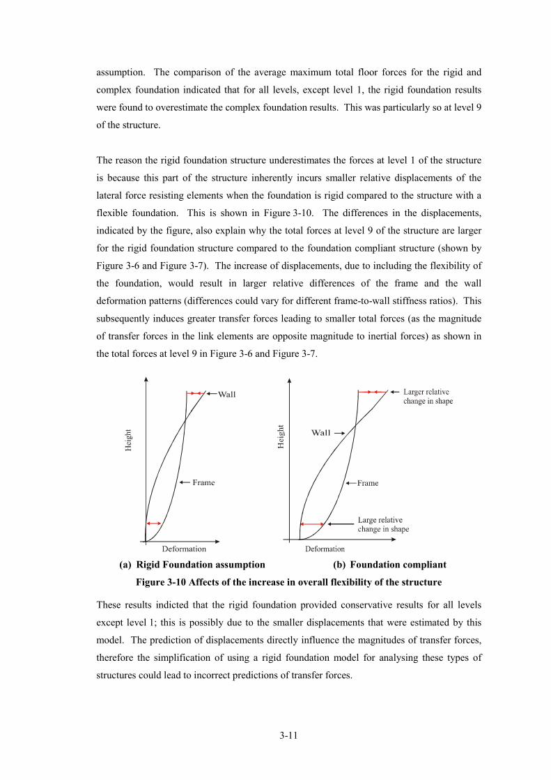
3�11

assumption. The comparison of the average maximum total floor forces for the rigid and

complex foundation indicated that for all levels, except level 1, the rigid foundation results

were found to overestimate the complex foundation results. This was particularly so at level 9

of the structure.

The reason the rigid foundation structure underestimates the forces at level 1 of the structure

is because this part of the structure inherently incurs smaller relative displacements of the

lateral force resisting elements when the foundation is rigid compared to the structure with a

flexible foundation. This is shown in Figure 3�10. The differences in the displacements,

indicated by the figure, also explain why the total forces at level 9 of the structure are larger

for the rigid foundation structure compared to the foundation compliant structure (shown by

Figure 3�6 and Figure 3�7). The increase of displacements, due to including the flexibility of

the foundation, would result in larger relative differences of the frame and the wall

deformation patterns (differences could vary for different frame�to�wall stiffness ratios). This

subsequently induces greater transfer forces leading to smaller total forces (as the magnitude

of transfer forces in the link elements are opposite magnitude to inertial forces) as shown in

the total forces at level 9 in Figure 3�6 and Figure 3�7.

(a) Rigid Foundation assumption (b) Foundation compliant

Figure 3%10 Affects of the increase in overall flexibility of the structure

These results indicted that the rigid foundation provided conservative results for all levels

except level 1; this is possibly due to the smaller displacements that were estimated by this

model. The prediction of displacements directly influence the magnitudes of transfer forces,

therefore the simplification of using a rigid foundation model for analysing these types of

structures could lead to incorrect predictions of transfer forces.

3�12

0 1000 2000

1

2

3

4

5

6

7

8

9

Level

Force (kN)

Comparison of maximum average envelope of transfer forces between a structure with

foundation compliance and a structure with rigid foundation assumption � SR 1:0.85

No FC

FC

0 500 1000 1500

1

2

3

4

5

6

7

8

9

Level

Force (kN)

Comparison of maximum average envelope of inertial forces between a structure with foundation


No FC

FC

Figure 3%11 Comparison of maximum

average envelope of transfer forces

between a structure with foundation

compliance and a structure with rigid

foundation assumption SR 1:0.85

Figure 3%12 Comparison of maximum

average envelope of inertial forces

between a structure with foundation

compliance and a structure with rigid

foundation assumption SR 1:0.85

Figure 3�11 and Figure 3�12 provide comparisons between the magnitude of transfer and

inertial forces for the rigid and complex foundations. The transfer and inertial floor force

results shown here, for the stiffness ratio of SR 1:0.85 were similar for the structures with

stiffness ratios of SR 1:1.69. These figures indicate that the underestimation of total floor

forces for the rigid foundation assumption at level 1 is due to the poor estimation of transfer

forces at level 1. Transfer forces are poorly estimated due to the increase in displacements

which occur for the complex foundation structure, as described above and shown in

Figure 3�10.

These figures also indicate that the inertial forces are overestimated by the structure with the

rigid foundation assumption. The inertial forces are overestimated by the structure with the

rigid foundation assumption due to the shorter fundamental period of the structure, compared

to the structure which includes the foundation flexibility. The shorter period, stiffer structure,

induces larger acceleration or inertial forces in accordance with the acceleration response

spectra.

3.1.3 9%Storey Flexible Structures Results: Total and Components of

Total Forces

Comparisons were made between results for the flexible 9�storey structure with different

foundation models. These comparisons were made to determine the affects of the flexibility

of the structure on the results for different foundation models.

3�13

0 1000 2000 3000

1

2

3

4

5

6

7

8

9

Level

Force

(kN)

Comparison of average peak total forces for structures with different foundation models

for 9�storey flexible structure � SR 1:0.85

No FC

FC

0 1000 2000 3000

1

2

3

4

5

6

7

8

9

Level

Force (kN)

Comparison of average peak total forces for structures with different foundation models

for 9�storey flexible structure � SR 1:1.69

No FC

FC

Figure 3%13 Comparison of average peak

total forces for structures with different

foundation models for 9%storey flexible

structure % SR 1:0.85



foundation models for 9%storey flexible


0 1000 2000 3000

1

3

5

7

9

Level

Force

(kN)

Comparison of average peak total forces for structures with different

foundation models for 9�storey flexible structure � SR 1:0.85

SF

FC

0 1000 2000 3000

1

3

5

7

9

Level

Force (kN)

Comparison of average peak total forces for structures with different

foundation models for 9�storey flexible structure � SR 1:1.69

SF

FC



foundation models for 9%sotrey flexible




foundation models for 9%sotrey flexible

structure % 1:1.69

Figure 3�13 to Figure 3�16 provide comparisons between the total floor forces for the

different foundation models for the 9�storey flexible structures. These results indicate that the

simple foundation model provided poor comparisons to the complex foundation model.

These figures show that the rigid foundation floor force results predict values that are greater

than the complex foundation floor results for all levels except level 8. This is different to the

results for the stiffer structures where level 1 was underestimated. The under prediction of

forces at level 8 for the rigid foundation structure is most likely due to the greater flexibility

3�14

of this structure. Greater structural flexibility results in larger deformations of both the frame

and wall elements at the upper levels of the structure and therefore results in larger transfer

forces.

The pattern of total forces is also slightly different for these flexible structures compared to

the results for the stiffer structures, described in Section 3.1.2. The inertial forces in general

are shown to decrease up until level 7 of the structure (shown in Figure 3�18), whereas for the

stiffer structures the inertial follow the more typical pattern of increasing with increasing

height of the structure (Figure 3�12). Figure 3�18 provides a comparison between the inertial

forces obtained for both a model with a rigid foundation and a model with a complex

foundation. These results both indicate this pattern of inertial forces which decrease with

height. This indicates that this pattern is not due to the foundation but due to the flexibility of

the structure.

0 500 1000 1500

1

3

5

7

9

Level

Force (kN)

Comparison of average peak transfer forces for structures with different foundation models for

9�storey flexible structure � SR 1:0.85

No FC

FC

0 500 1000 1500

1

3

5

7

9

Level

Force(kN)

Comparison of average peak inertia forces for structures with different foundation models for

9�storey flexible structure � SR 1:0.85

No FC

FC


transfer forces for structures with

different foundation models for 9%storey

flexible structure % SR 1:0.85


inertial forces for structures with

different foundation models for 9%storey

flexible structure % SR 1:0.85

Figure 3�17 and Figure 3�18 provide a typical indication of the comparisons between the

inertial and transfer floor force components for rigid and complex foundations for all the

range of different stiffness ratios discussed here. These figures show similar trends, to those

observed, for the 9�storey stiff structures.

These figures indicate that the magnitude of transfer forces are generally larger, at level 8 and

level 1, for the structural model which considers the flexibility of the foundation of the

structure compared to the results for the results for the rigid foundation. The inertial forces

3�15

were shown to be larger at level 8 for the structure which considers the flexibility of the

foundation.

The results from the 9�storey study have indicated that there are no benefits from using a

simple foundation model assumption compared to a rigid foundation model to represent the

real structural behaviour. These results have indicated that the rigid foundation assumption

fails to accurately predict the displacements, and consequently transfer forces, compared to

the complex foundation results.

Results for the comparisons between the foundation models for the 3 and 6 storey structures

are shown in Appendix B.1.1 and B.1.2. These results only show the comparisons between

the rigid foundations and the complex foundations as no benefits are observed by the rigid

foundation model.

3.1.4 Tower%to%Podium Structure with Foundation Compliance

To ensure realistic conclusions were drawn from the study on tower�to�podium structures,

foundation compliance was added to the tower�to�podium analytical models. The foundation

compliance model, developed in Section 3.1, was used to represent the foundation. The same

parameters that were used to represent the complex analytical foundation model were used for

this model.

Both the 9�storey tower and 3 and 6�storey�podium structures were used in this analysis with

stiffness ratios of SR 1:4.9 and SR 1:9.9 for the 3�storey podium structure and SR1:1.8 and

SR1:3.3 for the 6�storey podium structure. The twelve Wellington time history records,

described in Section 2.2.6 were used to investigate the response of the structure in this

section. The k1 scale factors used in these analyses are provided in Table 3�8.

Table 3%8 Scale factors for the earthquake records used in the podium%foundation

analyses for 3 and 6%storey wall structure

k1 3�storey wall k1 6�storey wall

Record Comp. SR1:4.9 SR1:9.9 SR1:1.8 SR1:3.3

Lucerne North 0.88 0.86 0.86 0.84

Lucerne South 1.47 1.49 1.49 1.50

Izmit North 1.71 1.70 1.70 1.68

Izmit South 1.60 1.58 1.58 1.54

La Union North 1.60 1.62 1.62 1.63

La Union South 2.61 2.67 2.67 2.71

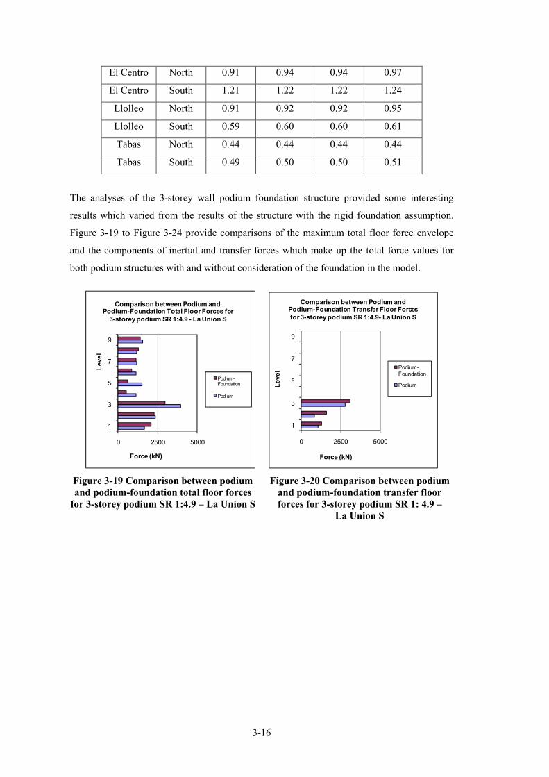
3�16

El Centro North 0.91 0.94 0.94 0.97

El Centro South 1.21 1.22 1.22 1.24

Llolleo North 0.91 0.92 0.92 0.95

Llolleo South 0.59 0.60 0.60 0.61

Tabas North 0.44 0.44 0.44 0.44

Tabas South 0.49 0.50 0.50 0.51

The analyses of the 3�storey wall podium foundation structure provided some interesting

results which varied from the results of the structure with the rigid foundation assumption.

Figure 3�19 to Figure 3�24 provide comparisons of the maximum total floor force envelope

and the components of inertial and transfer forces which make up the total force values for

both podium structures with and without consideration of the foundation in the model.

0 2500 5000

1

3

5

7

9

Force (kN)

Level

Comparison between Podium and Podium�Foundation Total Floor Forces for

3�storey podium SR 1:4.9 � La Union S

Podium'Foundation

Podium

0 2500 5000

1

3

5

7

9

Force (kN)

Level

Comparison between Podium and Podium�Foundation Transfer Floor Forces

for 3�storey podium SR 1:4.9� La Union S

Podium'

Foundation

Podium

Figure 3%19 Comparison between podium

and podium%foundation total floor forces

for 3%storey podium SR 1:4.9 – La Union S


and podium%foundation transfer floor

forces for 3%storey podium SR 1: 4.9 –

La Union S

3�17

0 2500 5000

1

3

5

7

9

Force (kN)

Level

Comparison between Podium and Podium�Foundation Inertial Floor Forces

for 3�storey podium SR 1:4.9 � La Union S

Podium'Foundation

Podium

0 2500 5000

1

3

5

7

9

Force (kN)

Level


3�storey podium SR 1:9.9 � La Union S

Podium'Foundation

Podium


and podium%foundation inertial floor forces

for 3%storey podium SR 1: 4.9 – La Union S




0 2500 5000

1

3

5

7

9

Force (kN)

Level



Podium'Foundation

Podium

0 2500 5000

1

3

5

7

9

Force (kN)

Level

Comparison between Podium and Podium�Foundation Inertial Floor Forces


Podium'Foundation

Podium


and podium%foundation transfer floor forces

for 3%storey podium SR 1: 9.9 – La Union S

Figure 3%24 Differences due to including

a foundation model on the inertia floor

forces results for SR 1: 9.9 – La Union S

Table 3%9 Summary of podium structure floor force values and podium%foundation

structure floor force values for 9%storey tower and 3%storey podium

Transfer Force Inertial Force Total Force

Lucerne N Generally greater for

PF structure

Generally greater for

P structure

Generally greater

for P structure

Lucerne S Generally greater for P

structure


P structure

Generally greater

for P structure

Izmit N Generally greater for P

structure


P structure

Generally greater

for P structure

Izmit S * * *

La Union N Generally greater for

PF structure

Greater for P

structure, PF greater

for upper levels (7�9)

Similar, P larger for

levels 4�5 and PF

larger for 7�9

3�18

La Union S Generally greater for

PF structure


P structure

Slightly greater for

P structure

El Centro N Generally greater for

PF structure

Greater for P structure

SR 1:4.9, 1:9.9

Similar for both P

and PF

El Centro S Slightly greater for PF

structure


P structure

Generally greater

for P structure

Llolleo N PF greater for levels 1

and 2


P structure

Generally greater

for P structure

Llolleo S Similar for both P and

PF


P structure

Generally greater

for P structure

Tabas N PF larger in general

especially for SR1:9.9


P structure

Generally greater

for P structure

Tabas S PF larger in general

especially for SR1:9.9


P structure

Generally greater

for P structure

Key: P= Podium structure with rigid foundation, PF=Podium structure with foundation

compliance, SR=Stiffness ratio

A summary of the comparisons made between the podium structure results and the podium�

foundation structure results for the time history records is provided in Table 3�9.

* Results for Izmit S were not included. The spectral acceleration of the Izmit S

component is above the design spectrum envelope at and around the fundamental

translational period for the structure. This is show in Figure 3�25.

Scaled Time History Records to T=1.140s

0

0.5

1

1.5

2

2.5

3

3.5

0 1 2 3 4

Time (s)

Accele

ration (g)

Satarget

Elcentro

Lucerne

Izmit

LaUnion

Chile

Iran

Figure 3%25 Spectral acceleration records for each of the south component time

history events

These large accelerations resulted in large demands on the structure and required the

strengths of the members in the structure to be increased to obtain acceptable results.

If the member strengths were adjusted then a direct comparison between the results of

the structures could not be made, therefore the results of Izmit�S were neglected.

The general trends found from these results, shown in Figure 3�19 to Figure 3�24 indicate

similar distribution of total forces for both the podium structures with and without foundation

compliance. The magnitudes were found to vary though. In general, the magnitudes of total

3�19

forces were found to be less for the podium structures which includes foundation flexibility

compared to structures with a rigid foundation assumption. The inertial force comparisons

generally indicated a decrease in the magnitude of inertial forces for the analytical models

included the foundation. This is expected due to the increase in flexibility of this structure

and therefore a decrease in the accelerations which develop in the floors of the structure. The

transfer force comparisons showed that, in some cases, the magnitudes of transfer forces were

larger for the foundation compliant podium structures compared to the non�compliant podium

structures. This increase was due to the increase in flexibility of the structure which caused

larger deformations of the lateral force resisting elements and therefore increases the transfer

forces.

A selection of the results for the 6�storey podium 9�storey frame structures are provided in

Figure 3�26 to Figure 3�31. These results are from the La Union 2 time history record. The

results for the other time history records were found to have similar results to the results

shown.

0 2000 4000

1

3

5

7

9

Force (kN)

Level


6 storey podium SR 1:1.8 � La Union S

Podium'

Foundation

Podium

0 2000 4000

1

3

5

7

9

Force (kN)

Level


for 6 storey podium SR 1:1.8 La Union S

Podium'

Foundation

Podium






forces for 6%storey podium SR 1:1.8 –

La Union S

3�20

0 2000 4000

1

3

5

7

9

Force (kN)

Level

Comparison between Podium and Podium�Foundation Inertia Floor Forces

for 6 storey podium SR 1:1.8 � La Union S

Podium'

Foundation

Podium

0 2000 4000

1

3

5

7

9

Force (kN)

Level


6 storey podium SR 1:3.3� La Union S

Podium'

Foundation

Podium


and podium%foundation inertial floor forces




for 6%storey podium SR 1: 3.3– La Union S

0 2000 4000

1

3

5

7

9

Force (kN)

Le

vel

Comparison between Podium and Podium�Foundation Transfer Floor for 6 storey

podium Forces SR 1:3.3 La Union S

Podium'

Foundation

Podium

0 2000 4000

1

3

5

7

9

Force (kN)

Leve

l

Comparison between Podium and Podium�Foundation Inertia Floor Forces

for 6 storey podium SR 1:3.3 � La Union S

Podium'

Foundation

Podium



forces for 6%storey podium SR 1: 3.3 –

La Union S


and podium%foundation inertial floor

forces for 6%storey podium SR 1:3.3 –

La Union S

Table 3%10 Summary of podium structure floor force values and podium%foundation

structure floor force values 9%storey two and 6%storey podium

Transfer Force Inertial Force Total Force

Lucerne N Similar, PF greater for

level 6 P greater for

level 1

Generally greater for P

structure


structure

Lucerne S Generally greater for P

structure


structure


structure

Izmit N P generally larger for

larger SR values


structure


structure

Izmit S � � �

La Union N P generally larger P larger for lower P larger for lower

3�21

especially level 1 levels PF larger for

upper levels

levels PF larger for

upper levels

La Union S Generally greater for P

structure

Greater for P structure,

PF slightly greater at

upper levels


PF slightly greater at

upper levels

El Centro N PF generally greater, P

greater for Level 1, 6

PF slightly larger than

F values

PF generally greater

except for levels 1, 6

El Centro S Greater for P structure Generally greater for P

structure


structure

Llolleo N Greater for P structure

especially for level 1


PF greater at upper

levels SR1:3.3


structure

Llolleo S Generally greater for P

structure


structure


structure

Tabas N Generally greater for P

structure


structure


structure

Tabas S Greater for P structure,

PF larger for SR1:3.3

at levels 1 and 6


PF larger at levels 8, 9

for SR 1:3.3


structure

Key: P= Podium structure rigid foundation, PF=Podium structure with foundation compliance.

A summary of the comparisons made between the podium structure results and the podium�

foundation structure results for all the time history records is provided in Table 3�10. Further

results for the 3 and 6 storey podium structures are presented in Appendix B.1.3.

These results indicate that for the 6�storey tower podium structures larger transfer, inertia and

total forces were found when the foundation was not considered in the analysis. This makes

sense for inertial forces as when foundation compliance is considered the flexibility of the

structure increases reducing the accelerations and consequently the inertial forces. For the

transfer forces, this result is different to what was observed for the 3�storey wall podium

structure. The reason the transfer forces were greater for this structure is possibly due to the

larger height of the wall of this structure. For the 3�storey podium structure the short wall is

relatively stiff compared to the more flexible 6�storey wall in the 6�storey podium structure.

The relative larger flexibility of the wall in the 6�storey podium structure causes these

observed smaller transfer forces.

3.2 Shear Deformation

To accurately model the behaviour of shear walls considerations should be given to both the

development of flexural and shear deformations in the wall. Typically, in non�linear

modelling, flexural deformations of walls are modelled well, whereas shear deformations are

not modelled so well due to the complex nature of how shear walls deform. Shear

3�22

deformations have been ignored in this study up until this point, the sensitivity of including

shear deformations into the models was investigated in this section.

To model shear deformations in walls a variety of considerations need to be made. Paulay

and Priestley (1992) suggest that the following items need to be considered: failure due to

diagonal tension or compression within the concrete caused by shear, sliding shear along

construction joints, and bond failure along lapped splices or anchorages. Only approximate

methods are currently available to model shear deformations and the complexities suggested

in Paulay and Priestley (1992) are not typically accounted for.

Research that has been carried out on shear deformations relates shear deformations of the

wall to the cyclic ductility of the wall. The analytical modelling program, RUAUMOKO

represents shear deformations by the use of ductility limits. RUAUMOKO requires

parameters which describe the ductility level at which strength degradation starts and where it

stops. Ductility values that were used for this research were obtained from the empirical

hysteresis model developed in Kelly (2004). The values were a ductility of 1.7 for the starting

strength degradation value and a ductility of 4.4 as the stopping strength degradation value.

Parameters are also required to describe the stiffness degradation of the member after

cracking of the concrete and yielding of the longitudinal and shear reinforcement has occurred

were also obtained from the hysteresis model described in Kelly (2004).

The models that were employed in these analyses were the same as the models used for the 9�

storey wall�to�wall structures and 9�storey frame�to�wall structures with a structural ductility

of 3 and fundamental translational periods of T=0.48s and T=0.58s respectively. The

softening action due to the shear deformations was thought to have the largest effect on the

stiffer group of structures and also the shear deformations are expected to be largest in these

structures.


Frame%to%Wall Structures

The results from this study indicate that there are some differences between the magnitudes of

forces which develop in the floor diaphragm when shear deformations are and are not

included in the model. The following figures represent the average of the peak total forces

and components of total forces (inertia and transfer forces) for frame�to�wall structures.

3�23

0 1000 2000 3000

1

3

5

7

9

Force (kN)

Lev

el

Comparison between average peak total floor forces for including and excluding shear deformation for 9�

storey stiff structure � SR1:0.85

No SD

SD

0 2000 4000

1

3

5

7

9

Force (kN)

Level

Comparison between average peak total floor forces for including and excluding shear deformation for 9�


No SD

SD

Figure 3%32 Comparison between average

peak total floor forces including and

excluding shear deformations for 9%storey

stiff structure – SR1:0.85


peak total floor forces including and

excluding shear deformations for 9%storey

stiff structure – SR1:1.69

“SD” refers to the results from the analytical model where shear deformations are included

and “No SD” refers to the model where shear deformations are excluded. Figure 3�32 and

Figure 3�33 show that excluding shear deformations in the analytical model results in slightly

larger total forces, than the total forces obtained from including shear deformations, for the

upper levels of the 9�storey structures and smaller total forces for the lower levels. It was

found that typically the effect on the forces, at the lower levels of the structure, was related to

the earthquake instead of the relative stiffness of the structure. Table 3�11 provides a

summary of which model provided the largest total forces at level 1 of the structure for the

different stiffness ratios and time�history records used in the study.

Table 3%11 Largest magnitudes of total force at level 1 for model with and without

consideration for shear deformation for 9%storey frame%to%wall structure

SR 1:0.85 SR 1:1.69

El Centro No SD No SD

Lucerne SD SD

Izmit SD No SD

La Union No SD No SD

Llolleo No SD No SD

Tabas SD SD

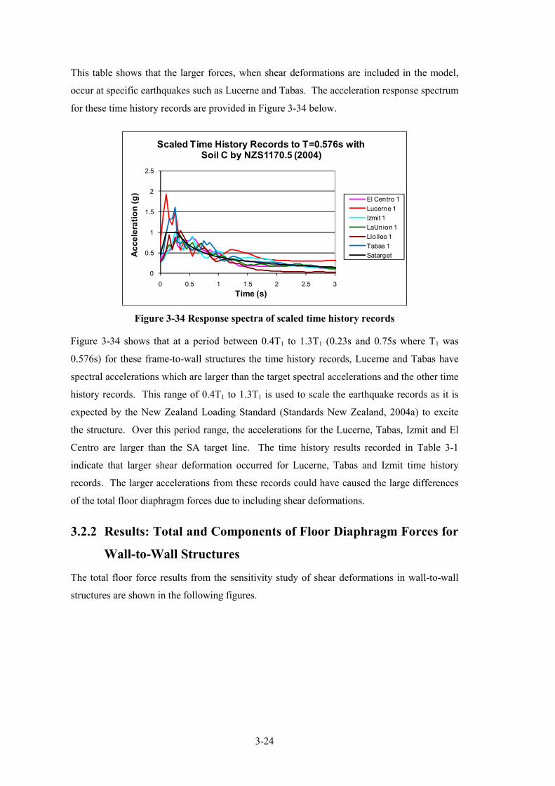
3�24

This table shows that the larger forces, when shear deformations are included in the model,

occur at specific earthquakes such as Lucerne and Tabas. The acceleration response spectrum

for these time history records are provided in Figure 3�34 below.

0

0.5

1

1.5

2

2.5

0 0.5 1 1.5 2 2.5 3

Ac

ce

lera

tio

n (

g)

Time (s)

Scaled Time History Records to T=0.576s with Soil C by NZS1170.5 (2004)

El Centro 1

Lucerne 1

Izmit 1

LaUnion 1

Llolleo 1

Tabas 1

Satarget

Figure 3%34 Response spectra of scaled time history records

Figure 3�34 shows that at a period between 0.4T1 to 1.3T1 (0.23s and 0.75s where T1 was

0.576s) for these frame�to�wall structures the time history records, Lucerne and Tabas have

spectral accelerations which are larger than the target spectral accelerations and the other time

history records. This range of 0.4T1 to 1.3T1 is used to scale the earthquake records as it is

expected by the New Zealand Loading Standard (Standards New Zealand, 2004a) to excite

the structure. Over this period range, the accelerations for the Lucerne, Tabas, Izmit and El

Centro are larger than the SA target line. The time history results recorded in Table 3�1

indicate that larger shear deformation occurred for Lucerne, Tabas and Izmit time history

records. The larger accelerations from these records could have caused the large differences

of the total floor diaphragm forces due to including shear deformations.


Wall%to%Wall Structures

The total floor force results from the sensitivity study of shear deformations in wall�to�wall

structures are shown in the following figures.

3�25

0 1000 2000 3000

1

3

5

7

9

Force (kN)

Level

Comparison between average peak total

floor forces for including and excluding shear deformation for 9�storey wall

structures � SR1:4

No SD

SD

0 1000 2000 3000

1

3

5

7

9

Force (kN)

Level

Comparison between average peak total

floor forces for including and excluding shear deformation for 9�storey wall

structures � SR1:14

No SD

SD


peak total floor forces for including and

excluding shear deformation for 9%storey

wall structures – SR1:4





0 1000 2000

1

3

5

7

9

Force (kN)

Lev

el

Comparison between average peak total floor forces for including and excluding

shear deformation for 9�storey wall structures � SR1:24

No SD

SD

0 1000 2000

1

3

5

7

9

Force (kN)

Lev

el

Comparison between average peak total floor forces for including and excluding

shear deformation for 9�storey wall structures � SR1:107

No SD

SD









Figure 3�35 to Figure 3�38 shows the variation in the distribution of average peak total forces

that was observed to occur between structures where shear deformations were and were not

included in the analytical model. A summary of the comparisons between the magnitude of

the total floor forces at level one of the structure for the model with and without shear

deformation for all the time history records is provided in Table 3�12.

3�26

Table 3%12 Largest magnitudes of total force at level 1 for different shear deformation

models for wall%to%wall structures

Wall�to�Wall Stiffness Ratios

1:232 1:107 1:45 1:24 1:14 1:9 1:6 1:4 1:2

Izmit 1 S SD S S SD No SD S No SD S

Tabas 1 S S S S No SD No SD S No SD No SD

Llolleo 1 S SD SD S No SD S S No SD S

Llolleo 2 S SD SD S S SD S No SD S

LaUnion 1 S S S S No SD S S S S

ElCentro 1 S S SD S SD No SD S No SD S

The label “S” in this table refers to the magnitude of the total floor force at level 1 of the

structure being similar for both structures which include and excluded shear deformations in

the analysis.

The results from Table 3�12 show that the trends are not as clear as they were for the frame�

to�wall structures. The blurred trends for these wall�to�wall structures are possibly a result of

shear deformations developing in both walls. The general trends shown in Figure 3�35 to

Figure 3�38 indicate for large wall�to�wall stiffness ratios (greater than SR1:24) larger total

floor diaphragm forces develop at level 1 of the structure for a model which includes shear

deformations for one which excludes shear deformations. The reason larger forces develop

for these structures is due to the changes in the relative stiffness of both of the walls. With a

large stiffness ratio one wall is much stiffer (or longer) than the other wall. Large shear

deformation would be expected to develop in the longer wall due to the smaller height�to�

length ratio of the longer wall. The larger shear deformations in the longer wall would reduce

the stiffness of the wall making the stiffness more similar to the stiffness of the shorter wall.

Initially, before shear deformations developed in the wall, the shorter wall is much more

flexible relative to the longer wall. Therefore, the magnitude of transfer forces which

developed between these walls is reasonably small as the shorter wall typically conforms to

deformations of the longer wall as it was relatively very flexible. After shear deformations

developed in the longer wall the relative stiffness between the two walls reduces and therefore

larger transfer forces develop, as seen in Section 2.3.10 for wall�to�wall interaction. This

explains why larger total forces develop for walls with larger stiffness ratios.

For small stiffness ratios (less than SR1:24) the results from the analytical model, where shear

deformations were neglected, were found to have larger total forces at level 1 of the structure

in comparison to the results from the model which incorporates the effects of shear

3�27

deformations. This is due to slightly larger shear deformations developing in the longer of the

two walls causing the stiffness of the two walls to become more similar. For walls with

similar stiffness transfer forces would be very small as the walls will deform similarly.

Additional results to the results shown are provided in Appendix B.3 for 3, 6 and 9 storey

wall�to�wall structures.

3.3 Plastic Hinge Model

Research carried out by Beyer (2005), which is described in the literature review in

Section 2.1.5, found that when modelling walls of different lengths, the lumped plasticity

assumption used to represent the plastic hinges in walls can lead to inaccurate results. This

section will provide comparisons between the results from lumped plasticity hinge models

and distributed plasticity hinge models for the walls in the frame�to�wall and wall�to�wall

structures.

The same structures will be used here as was used in previous analyses in this research. The

frame�to�wall structures of 9, 6 and 3�storey, stiffness ratios of SR1:0.85 and SR1:1.69 for the

9�storey structures, SR1:1.49 and SR1:3.51 for the 6�storey structures and SR1:0.3 and

SR1:1.14 for the 3�storey structures were included in this study. The fundamental periods of

9, 6 and 3�storey stiff structures that were used are respectively; T1 9storey=0.576s, T1

6storey=0.321s and T1 3storey=0.275s. The 9�storey flexible structure with a fundamental period

of T1 9storey=1.437s was also used in this study. The 9�storey flexible structure was included in

this study to check that what differences may have occurred in the results. It was expected

that similar results would be achieved as the stiffness ratios between the components were the

same.

The wall�to�wall structures used for this study were the 9�storey structures with the following

stiffness ratios; SR1:6, SR1:14, and SR1:45. Only the 9�storey wall�to�wall structures were

included in this study as the study by Beyer (2005) provides a reasonably comprehensive

sensitivity study on plastic hinge types for wall structures.

3�28

Possible hinge

location

M1M2

(1�r).E.I

ar.E.I EI

ArEI1

1

Beam

Figure 3%39 Two component beam model

Where Mx, represents the applied moment, r represents the bi�linear factor, E represents the

elastic modulus of the beam and I represents the second moment of area for the beam. The

lumped plasticity hinges used in previous studies were modelled by using the two component

beam model represented in Figure 3�39. This model has two elements which represent the

elastic perfectly plastic behaviour and the strain hardening behaviour.

The distributed plasticity in the hinge zones were modelled in this study by using a plastic

hinge element that was developed by Peng (2009) in parallel with a multi�spring element.

This plastic hinge element was used to represent the concrete strength and stiffness

contribution of the wall and to also model the core, cover and shear components of the

concrete. The element has the ability to model the longitudinal steel bars in typical beam

sections, but not the distributed of reinforcing bars, typical of larger wall type sections. To

model the distributed reinforcing bars of walls, the multi�spring element was used.

Figure 3�40 provides a representation of the configuration of the elements used to model the

distributed plasticity in the hinge zone.

NodeBrian Peng Hinge Multi spring

Figure 3%40 Distributed plasticity model

3�29

Eight of these elements were vertically connected in series to represent the segment of wall

between the floors of the structure. Multiple elements were used to ensure an accurate

response of the wall was captured. The hinge element and the multi�spring element were

connected in parallel to ensure strain compatibility was maintained between the concrete and

the steel material. The inelastic action of the concrete was modelled using the concrete

hysteresis model (Peng, 2009) that was available in RUAUMOKO. A bi�linear hysteresis

model was used to represent the behaviour of the reinforcing steel in the multi�spring element.

Extensive verification of this plastic hinge model for beam elements has been carried out and

is described by Peng (2009). However, the configuration of the plastic hinge element

combined with a multi�spring element to represent the response of a reinforced concrete wall

has not been verified. Therefore a verification study was carried out by comparing the

response of an analytical wall model, which included the Peng hinge element and the multi�

spring element, to some results obtained from an external experimental study which was

carried out by Elnashai et al. (1990) on the behaviour of reinforced concrete walls. Nine

different wall specimens were constructed and tested in that experimental study. Each wall

had a varying proportion of longitudinal and transverse reinforcement. The experimental

results for two of the walls were compared to the analytical results from a push�over analysis

for walls with similar parameters. The geometry of these walls was 1.2m high, 0.6m long and

0.06m wide. The first wall (referred to latter as wall 1) contained 2.83% flexural

reinforcement and 0.39% shear reinforcement and the second wall (referred to later as wall 2)

contained 2.93% flexural reinforcement and 0.56% shear reinforcement. The comparisons of

the hysteresis loops from this experiment and to the analytical results produced here are

shown in Figure 3�41 and Figure 3�42.

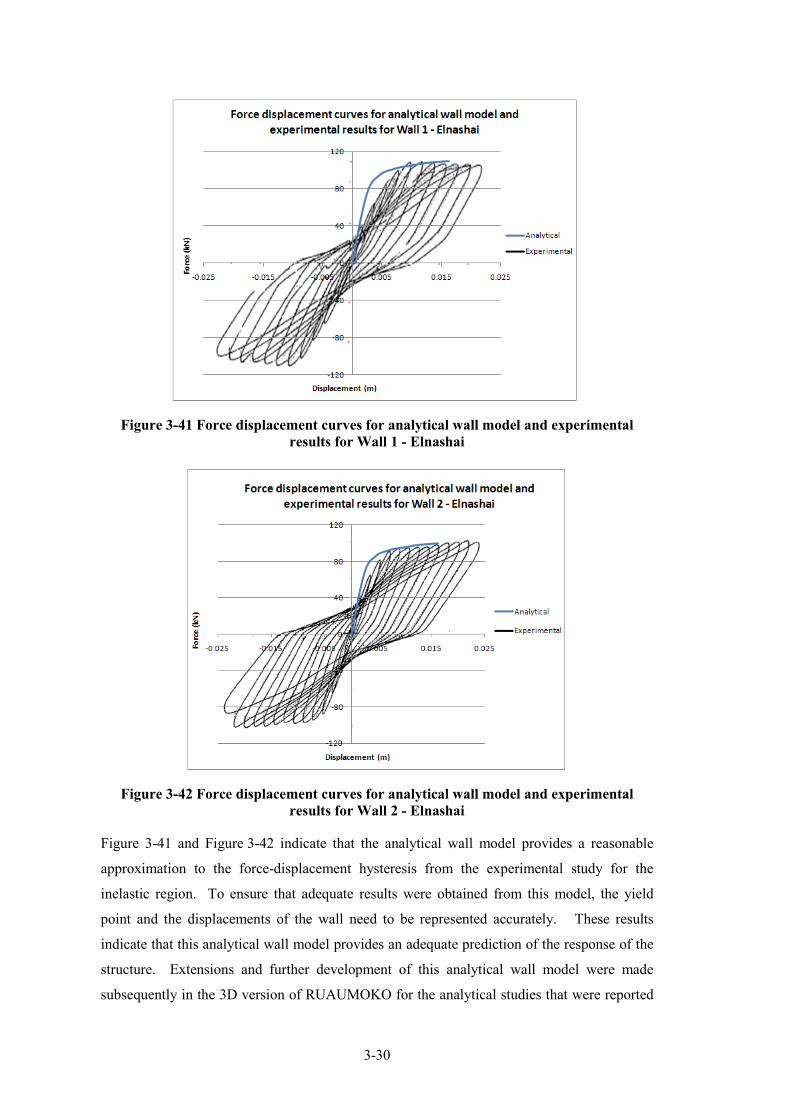
3�30

Figure 3%41 Force displacement curves for analytical wall model and experimental

results for Wall 1 % Elnashai

Figure 3%42 Force displacement curves for analytical wall model and experimental

results for Wall 2 % Elnashai

Figure 3�41 and Figure 3�42 indicate that the analytical wall model provides a reasonable

approximation to the force�displacement hysteresis from the experimental study for the

inelastic region. To ensure that adequate results were obtained from this model, the yield

point and the displacements of the wall need to be represented accurately. These results

indicate that this analytical wall model provides an adequate prediction of the response of the

structure. Extensions and further development of this analytical wall model were made

subsequently in the 3D version of RUAUMOKO for the analytical studies that were reported

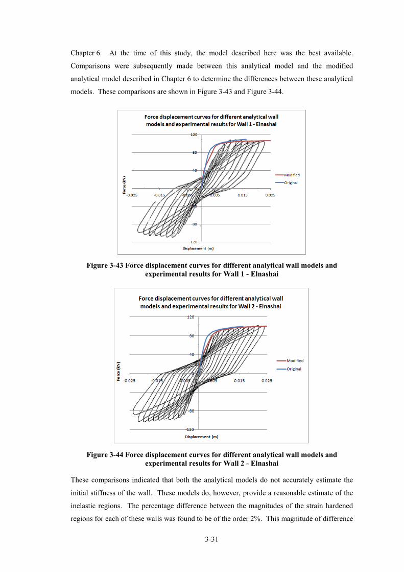
3�31

Chapter 6. At the time of this study, the model described here was the best available.

Comparisons were subsequently made between this analytical model and the modified

analytical model described in Chapter 6 to determine the differences between these analytical

models. These comparisons are shown in Figure 3�43 and Figure 3�44.

Figure 3%43 Force displacement curves for different analytical wall models and

experimental results for Wall 1 % Elnashai

Figure 3%44 Force displacement curves for different analytical wall models and

experimental results for Wall 2 % Elnashai

These comparisons indicated that both the analytical models do not accurately estimate the

initial stiffness of the wall. These models do, however, provide a reasonable estimate of the

inelastic regions. The percentage difference between the magnitudes of the strain hardened

regions for each of these walls was found to be of the order 2%. This magnitude of difference

3�32

between these two analytical models is within the errors of the analyses. This indicates that

the results from this original analytical wall model and the results from the modified

analytical wall model are comparable.

The parameters that were used in the hinge model to investigate the sensitivity of the lumped

hinge assumption are provided in Table 3�13 and Table 3�14.

Table 3%13 Frame%to%wall distributed plastic hinge parameters for stiff 9%storey

structure

Parameter SR1:0.85 SR1:1.69

Width (m) 0.4 0.4

Depth (m) 9.45 10.53

Cover (m) 0.05 0.05

Length of hinge (m) 3.00 3.10

Modulus of elasticity�Concrete (GPa) 26.5 26.5

Compressive strength f’c (MPa) 30.0 30.0

Tensile Strength ft (MPa) 2.2 2.2

Modulus of elasticity�Shear (GPa) 10.06 10.06

Compressive strength f’c –shear (MPa) 10.6 10.6

Modulus of elasticity –Steel (GPa) 200 200

Yield strength of reinforcement (MPa) 500 500

Effective depth of concrete strut (m) 2.86 2.98

Area of steel � total (m2) 6.03x10

�3 6.43x10

�3

The length of the hinge element and the effective depth of the structure, provided in Table

3�13 and Table 3�14, were determined from the procedure described in Chapter 6.

Similar parameters were used for the 3 and 6�storey structures. The area of the steel was

determined in accordance with the strength requirements of the NZ concrete design standard

(Standards New Zealand, 2006).

Table 3%14 Wall%to%wall distributed plastic hinge parameters for 9%storey wall structure

SR 1:6 SR 1:14 SR 1:45

Parameter Wall 1 Wall 2 Wall 1 Wall 2 Wall 1 Wall 2

Width (m) 0.4 0.4 0.4 0.4 0.4 0.4

Depth (m) 7.00 12.85 5.00 13.00 3.00 12.95

Cover (m) 0.05 0.05 0.05 0.05 0.05 0.05

3�33

Length of hinge (m) 2.75 3.34 2.55 3.35 2.35 3.35

Modulus of elasticity�

Concrete (GPa)

26.5 26.5 26.5 26.5 26.5 26.5

Compressive strength f’c

(MPa)

30.0 30.0 30.0 30.0 30.0 30.0

Tensile Strength ft (MPa) 2.2 2.2 2.2 2.2 2.2 2.2

Modulus of elasticity�

Shear (GPa)

10.06 10.06 10.06 10.06 10.06 10.06

Compressive shear

strength f’vc (MPa)

10.6 10.6 10.6 10.6 10.6 10.6

Tensile shear strength fvt

(MPa)

1.0 1.0 1.0 1.0 1.0 1.0

Modulus of elasticity –

Steel (GPa)

200 200 200 200 200 200

Yield strength of

reinforcement (MPa)

500 500 500 500 500 500

Effective depth of

concrete strut (m)

2.56 3.23 2.27 3.24 1.85 3.24

Area of steel � total (m2) 6.84x10

�3 0.0209 8.04x10

�3 0.0209 2.49x10

�3 0.0209

Comparisons were made between the base shear forces in the wall and columns for the 9�

storey stiff frame�to�wall model to verify that the distributed plastic hinge model was working

properly. Exact comparisons were not expected, however, similar trends were expected as the

initial stiffness should be similar.

'3000

'2000

'1000

0

1000

2000

3000

0 10 20 30 40

Ba

se

sh

ea

r (k

N)

Time (s)

Comparison of Base Shear in the Columns for Different Wall Hinge Plasticity Models � El Centro N

DPH

LH

Figure 3%45 Comparison of base shear in the wall for different wall hinge plasticity

models – El Centro N

These figures indicate that the distributed plastic hinge model provided reasonably

comparable shear forces to those of the lumped plasticity model. It is shown that for the

initial loading the base shear forces are similar, which is as expected. The differences in the

magnitudes of shear force, as time proceeds, is due to the changed plasticity of the wall for

each of the models.

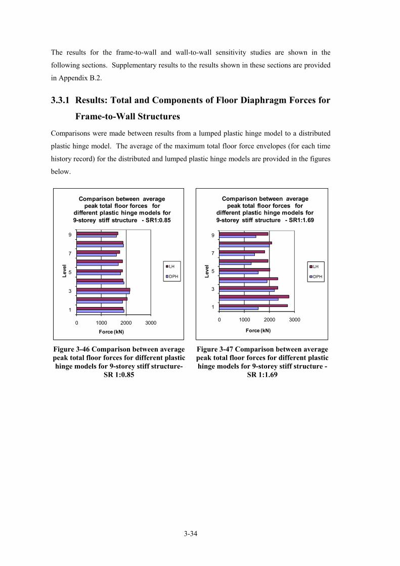
3�34

The results for the frame�to�wall and wall�to�wall sensitivity studies are shown in the

following sections. Supplementary results to the results shown in these sections are provided

in Appendix B.2.


Frame%to%Wall Structures

Comparisons were made between results from a lumped plastic hinge model to a distributed

plastic hinge model. The average of the maximum total floor force envelopes (for each time

history record) for the distributed and lumped plastic hinge models are provided in the figures

below.

0 1000 2000 3000

1

3

5

7

9

Force (kN)

Level

Comparison between average peak total floor forces for

different plastic hinge models for

9�storey stiff structure � SR1:0.85

LH

DPH

0 1000 2000 3000

1

3

5

7

9

Force (kN)

Level

Comparison between average peak total floor forces for

different plastic hinge models for


LH

DPH


peak total floor forces for different plastic

hinge models for 9%storey stiff structure%

SR 1:0.85



hinge models for 9%storey stiff structure %

SR 1:1.69

3�35

0 1000 2000 3000

1

3

5

7

9

Force (kN)

Leve

l

Comparison between average peak transfer component of floor forces

for different plastic hinge models for


LH

DPH

0 1000 2000 3000

1

3

5

7

9

Force (kN)

Lev

el

Comparison between average peak transfer component of floor forces

for different plastic hinge models for


LH

DPH


peak transfer component of floor forces

for different plastic hinge models for 9%

storey stiff structure % SR 1:0.85


average peak transfer component of floor

forces for different plastic hinge models

for 9%storey stiff structure – SR 1:1.69

0 1000 2000 3000

1

3

5

7

9

Force (kN)

Level

Comparison between average peak inertia component of floor forces for different plastic hinge models for 9�


LH

DPH

0 1000 2000 3000

1

3

5

7

9

Force (kN)

Level

Comparison between average peak inertia component of floor forces for different plastic hinge models for 9�


LH

DPH


peak inertia component of floor forces for

different plastic hinge models for 9%storey

stiff structure% SR 1:0.85


peak inertia component of floor forces for


stiff structure % SR 1:1.69

Note: DPH = Distributed plastic hinge, LH= Lumped plastic hinge

Figure 3�46 and Figure 3�47 provide a comparison between the total floor force results for the

two plastic hinge models and Figure 3�48 and Figure 3�49 provide a comparison between the

transfer forces and Figure 3�50 and Figure 3�51 provide a comparison between the inertial

forces. The most significant change in the total floor forces was observed at level 1 of the

structure for all stiffness ratios, which was where the most plastic deformation occurs. Both

the transfer and inertia components of total force were found to contribute to these large

changes of force at level 1 of the structure.

3�36

The magnitude of transfer and inertial forces were affected by the type of plastic hinge model

due to the different hinge models imposing different stiffness and deformation responses

elements. For the lumped hinge model, plasticity occurs at one point in the wall which

concentrates the deformation at one point and therefore induces large transfer forces. For the

distributed plastic hinge model, the plasticity is spread over a greater height of the wall. As

transfer forces develop due to differences in the deformation patterns, when the deformation

in the wall is more spread the development of transfer forces becomes less concentrated

(compared to the lumped plastic hinge model) and therefore affects the magnitudes of transfer

forces. This finding is similar to the findings reported in the wall study by Beyer (2005). The

response of the structure was found to sustain smaller inertial forces for the distributed plastic

hinge model as the spread of plasticity reduces the stiffness and subsequently the inertial

forces which develop in the floor. This indicates that the reduction in total forces is due to

both the reduction of transfer and inertial forces.

To ensure that these results do not differ for more flexible structures a study was carried out

on the sensitivity of the plastic hinge model for the 9�storey flexible structures. Similar

figures were developed for these results showing the maximum average total force

comparison between the floor force results for the lumped hinge and the distributed hinge

models.

0 1000 2000 3000

1

3

5

7

9

Force (kN)

Level

Comparison between average peak total floor forces for different plastic

hinge models for 9�storey flexible structure �SR 1:0.85

LPH

DPH

0 1000 2000 3000

1

3

5

7

9

Force (kN)

Lev

el

Comparison between average peak total floor forces for different plastic hinge

models for 9�storey flexible structure �SR 1:1.69

LPH

DPH



hinge models for 9%storey flexible structure

% SR 1:0.85



hinge models for 9%storey flexible



3�37

Figure 3�52 and Figure 3�53 show similar results for level 1 to those predicted for the stiff 9�

storey structure for the same level. The components of total force also indicated similar

trends, where both transfer and inertial forces were observed to reduce at level 1.

These figures indicate there is no significant sensitivity to the plastic hinge model for

structures of different flexibilities. Therefore only the stiff structures were included to

investigate the sensitivity for the 6 and the 3�storey structures. Similar results were obtained

for the 6 and the 3�storey structures as shown in Figure 3�54 to Figure 3�57.

0 1000 2000 3000

1

2

3

4

5

6

Force (kN)

Leve

l


models for 6�storey stiff structure � SR 1:0.61

LPH

DPH

'1000 0 1000 2000 3000

1

2

3

4

5

6

Force (kN)

Level


models for 6�storey stiff structure � SR 1:1.49

LPH

DPH




SR 1:0.61




SR 1:1.49

'1000 1000 3000

1

2

3

Force (kN)

Level

Comparison between average peak Inetia floor forces for different plastic

hinge models for 3�storey stiff structure � SR 1:0.3

No FC

FC

'1000 1000 3000

1

2

3

Force (kN)

Level

Comparison between average peak Inetia floor forces for different plastic

hinge models for 3�storey stiff structure � SR 1:1.14

No FC

FC




SR 1:0.30




SR 1:1.14

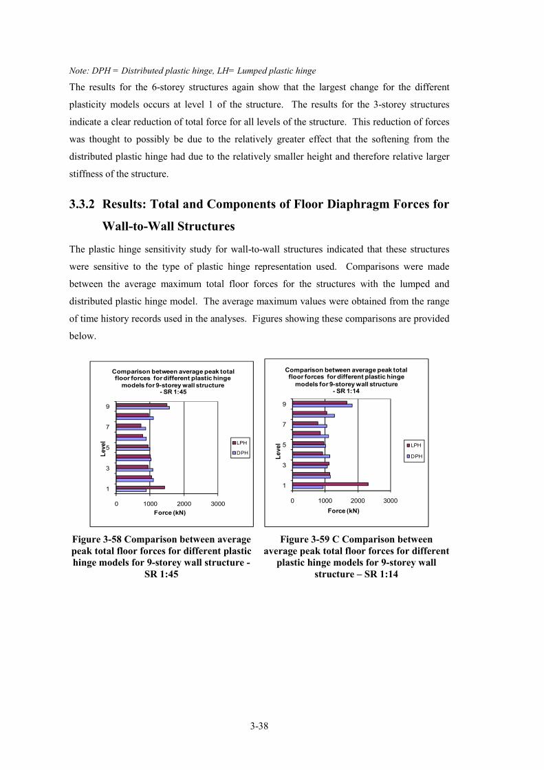
3�38


The results for the 6�storey structures again show that the largest change for the different

plasticity models occurs at level 1 of the structure. The results for the 3�storey structures

indicate a clear reduction of total force for all levels of the structure. This reduction of forces

was thought to possibly be due to the relatively greater effect that the softening from the

distributed plastic hinge had due to the relatively smaller height and therefore relative larger

stiffness of the structure.


Wall%to%Wall Structures

The plastic hinge sensitivity study for wall�to�wall structures indicated that these structures

were sensitive to the type of plastic hinge representation used. Comparisons were made

between the average maximum total floor forces for the structures with the lumped and

distributed plastic hinge model. The average maximum values were obtained from the range

of time history records used in the analyses. Figures showing these comparisons are provided

below.

0 1000 2000 3000

1

3

5

7

9

Force (kN)

Level


models for 9�storey wall structure � SR 1:45

LPH

DPH

0 1000 2000 3000

1

3

5

7

9

Force (kN)

Le

vel



LPH

DPH



hinge models for 9%storey wall structure %

SR 1:45

Figure 3%59 C Comparison between

average peak total floor forces for different

plastic hinge models for 9%storey wall

structure – SR 1:14

3�39

0 1000 2000 3000

1

3

5

7

9

Force (kN)

Level



LPH

DPH

0 1000 2000 3000

1

3

5

7

9

Force (kN)

Level

Comparison between average peak transfer floor forces for different

plastic hinge models for 9�storey wall structure � SR 1:14

LPH

DPH



hinge models for 9%storey wall structure –

SR 1:6


peak transfer floor forces for different

plastic hinge models for 9%storey wall

structure SR 1:14


0 1000 2000 3000

1

3

5

7

9

Force (kN)

Leve

l

Comparison between average peak transfer component of floor forces for different plastic hinge


LPH

DPH

0 1000 2000 3000

1

3

5

7

9

Force (kN)

Level

Comparison between average peak inertia component of floor forces for different plastic hinge models

for 9�storey wall structure � SR 1:45

LPH

DPH


peak transfer component of floor forces

for different plastic hinge models for 9%

storey wall structure – SR 1:6


peak transfer component of floor forces for


wall structure SR 1:14


Figure 3�58 to Figure 3�60 indicate that the magnitudes of total floor forces for level 1 of all

of the structures reduced greatly when the distributed plastic hinge model was employed

compared to the floor forces for the lumped plastic hinge model. Figure 3�68 and Figure 3�69

indicate the average transfer and inertial components of forces which made up the peak

average total forces for the 9�storey wall structure with wall�to�wall SR of 1:45. The

reduction of floor forces at level 1 for these wall�to�wall buildings was much larger than for

the frame�to�wall structures. Figure 3�68 indicates that the large reduction of total forces at

3�40

level 1 is due to a large reduction of transfer forces, Figure 3�69 indicates small differences of

inertial forces. This reduction is much larger compared to what was observed for the frame�

to�wall structures due to the larger stiffness values of the walls compared to frames and

further, after yielding the walls in the wall�to�wall structures the walls deform more similarly

to each other than the frames and walls of the dual structures.

The reduction of total forces and transfer forces due to including distributed plasticity in the

wall members found in this study are in line with the findings of Beyers’ (2005) work on

coupled wall structures.

3.4 Results Including: Foundation Flexibility, Shear

Deformation and Distributed Plastic Hinge Model

Models were developed and analysed which included all of the recommended modelling

parameters from the sensitivity study in Sections 3.1, 3.2 and 3.3. The parameters were:

− A complex foundation model which accounts for the flexibility of the foundation and

surrounding soil

− Shear deformation behaviour of the wall members

− Distributed representation of the plastic hinge behaviour of the columns and walls

members

These analytical models were thought to provide the most accurate estimate of the magnitudes

of floor diaphragm forces. The floor diaphragm forces obtained from these analyses were

used to develop the floor diaphragm static design method described in Chapter 5.

This study included structures located in the Wellington region and not the Auckland region

as analyses in Section 2.3.8, on transfer forces in low seismic regions, indicated that transfer

forces were found to be negligible. The magnitudes of the floor diaphragm forces from this

study, where the analytical models incorporated all of the modelling parameters that were

found to be sensitive to transfer forces, to develop the new static design method that is

discussed in Chapter 5.

To adequately verify the proposed static design, the behaviour of these structures needed to be

verified on different soil types. Three different soil types were included in this study, these

were: rock, shallow soil and deep or soft soil defined in the New Zealand Structural Design

Actions Standard (Standards New Zealand, 2004a). Very soft soil exists were not included in

this study. In the Wellington region all three of these soil types could exist: the Torlesse rock

outcrops could represent rock, the alluvium deposits in the CBD area could represent the

3�41

shallow soil regions and the deposits in the Lambton Quay/water front zone of marginal

marine sediments could represent the deep or soft soil sites (Begg and Mazengarb, 1996).

The member sizes, strengths and stiffness properties for the models on shallow soils are the

same as the values used for the same models in previous analyses. The strengths values used

in these models were based on probable strengths, as for the other analytical models. The

values for the structures on both rock and deep or soft soils were obtained in a similar way to

the methods described in previous chapters.

The foundation of the structures that were assumed to be located on rock ground was

modelled with rigid foundations. Where the structures were located on deep or soft soils a

pile foundation model was assumed similar to that described in Section 3.1. The differences

between deep and soft soils lay with the foundation strength and stiffness parameters. The

foundation parameters used to model the foundation at the Wellington waterfront were

obtained from a practicing senior geotechnical engineer. It was advised that the typical soil

conditions were a 10m thickness of end�dumped fill overlying dense gravels. The depth to

bed rock in this region was 150m (Murashev and Palmer, 1998). Standard Penetration Test

(SPT) blow count values for the fill and gravel were advised to be N=10 and N=50+

respectively. The sub�grade reaction for this soil type was obtained using Equation 3�6 and

the provided parameters.

75.0

056 −= NDk Equation 3%6

Where N= the SPT blow count value and Do represents the pile diameter.

Structures of 3, 6 and 9�storey with a range of flexibilities from stiff to flexible, designed for

structural ductility of 3, with frame�to�wall stiffness ratios of SR 1:0.85 and SR 1:1.69, were

analysed. The time history records were all scaled to match the seismicity of the Wellington

CBD area and the appropriate soil conditions.

The frame�to�wall stiffness ratios of SR1:0.85 and SR1:1.69 were used in the analyses of the

structures on the shallow soil. Only structures with a frame�to�wall stiffness ratio of 1:0.85

were only included in the analytical studies of the structures on both rock and soft or deep

soil. The results from the structures on shallow soils indicated that variations in the frame�to�

wall stiffness ratios did not greatly affect the results that were used to calibrate that static

design envelope. This is therefore why only structures with stiffness ratios of 1:0.85 were

included in the studies for structures on other soil types.

3�42

The fundamental periods for the structures on shallow foundations are provided in Table 3�15

and the periods for the structures on rock and deep foundation are provided in Table 3�15. It

was attempted to keep the fundamental periods for the buildings of similar heights, with

different stiffness ratios, the same to remove the dynamic affects between the behaviour of

these buildings.

Table 3%15 Fundamental periods for structures with shallow foundations

Structure SR T1

9�storey stiff 1:0.85 1.19

1:1.69 1.24

9�storey flex 1:0.85 1.79

1:1.69 1.87


1:1.49 0.93


1:1.49 1.12


1:1.14 0.77


1:1.14 0.83

Table 3%16 Fundamental periods for the structures on rock or deep/soft foundation

types

T1

Structure SR Rock Deep/soft

9�storey stiff 1:0.85 0.57 1.00

9�storey flex 1:0.85 1.30 1.60

6�storey stiff 1:0.61 0.37 0.72

6�storey flex 1:0.61 0.63 0.93

3�storey stiff 1:0.3 0.31 0.53

3�storey flex 1:0.3 0.60 0.85

The earthquake time history records that were incorporated into this study were the same as

the records described in Section 2.2.6.

3�43

3.4.1 Wellington Buildings

3.4.1.1 Floor Diaphragm Forces: 9%Storey Stiff Building

Comparisons were made between the components of total force for each of the different

stiffness ratios for the 9�storey stiff structure. The average maximum values from all of the

time history records have been used to make these comparisons. Figures showing these

comparisons are provided below for the structures on shallow soil.

0 1000 2000

1

2

3

4

5

6

7

8

9

Force (kN)

Le

ve

l

Comparison of Average Peak Components of Total Floor Forces for

the 9�storey stiff SR 1:0.85

Transfer

Inertia

Total

0 2000 4000

1

2

3

4

5

6

7

8

9

Force (kN)

Le

ve

l


the 9�storey stiff SR 1:1.69

Transfer

Inertia

Total


components of total floor force for the 9%

storey stiff – SR 1:0.85


components of total floor force for the 9%

storey stiff – SR 1:1.69

These comparisons indicate slightly different results to what has been observed in previous

analyses. The large magnitudes of transfer forces at the base of the structure (shown in the

results of Section 2.3) have disappeared as a result of the inclusion of distributed plastic hinge

zones in to the analytical model. The large forces that were identified in previous analyses

are still evident at level 8 of the structure. These forces are due to both the large transfer that

occurs due to the change in dominant vertical lateral force resisting element and the large

accelerations that occur with increasing height of the structure. The small forces at level 9 are

again observed in these figures. This force is due to the frame stiffness dominating the wall

stiffness at the upper levels and therefore the direction of transfer has changed. The transfer

forces at level 1 are shown to be less than the inertial forces. This is plausible due to the

relative displacements at the lower levels being less than the displacements at the upper

levels.

The distributions of the forces, shown in these figures, are different to the distribution of the

forces expected. The expected distribution of forces is a distribution that is similar an

3�44

Equivalent Static Analysis distribution. It is possible that the forces shown in these figures

are different to the expected distribution due to higher mode effects because the Equivalent

Static Analysis (ESA) method is based on a first mode response. To determine if this is the

case the distribution of forces, that make up these average maximum envelopes, from

different earthquakes at different times were graphed.

0

1

2

3

4

5

6

7

8

9

10

'2000 '1000 0 1000 2000 3000

Level

Force (kN)

Force distribution for maximum total forces at different times for 9�storey stiff

structure SR 1:0.85 � El Centro N

T=7.52s

T=16.82s

T=16.84s

T=16.88s

T=16.94s

T=16.96s

T=17.02s

T=17.62s

T=18.12s

Figure 3%66 Force distribution for maximum total forces at different times for 9%storey

stiff structure SR1:0.85– El Centro N

Figure 3�66 shows the distribution of force which relate to the maximum force envelope.

This figure indicates that the distribution of forces that developed in this structure is not based

on the fundamental mode shape of the structure. This explains why the distribution of forces

in the average maximum envelope figures above are different to the distributions of the ESA

method and further, why larger forces are observed to develop in the lower levels of the

structure.

3.4.1.2 Floor Diaphragm Forces: 9%Storey Flexible Building

Comparisons were made between the components of total force for each of the different

stiffness ratios for the 9�storey flexible structure. It is expected that some differences will be

observed compared to the results of the 9�storey stiff structures as differences existed in the

results between these two structures in the sensitivity study. The average maximum values

from all of the time history records have been used to make the comparisons between the total

forces. Figures showing these comparisons are provided below.

3�45

0 1000 2000

1

2

3

4

5

6

7

8

9

Force (kN)

Le

ve

l

Comparison of Average Peak Components of Total Floor Force for the

complete 9�storey flexible�SR 1:0.85

Transfer

Inertia

Total

0 1000 2000

1

2

3

4

5

6

7

8

9

Force (kN)

Le

ve

l

Comparison of Average Peak Components of Total Floor Force for

the complete 9�storey flexibleSR 1:1.69

Transfer

Inertia

Total


components of total floor force for the

complete 9%storey flexible– SR 1:0.85



complete 9%storey flexible – SR 1:1.69

These results indicated that for these structures, the forces at level 8 are relatively greater than

the forces at the levels below compared to the forces at level 8 for the stiff structure. This

result is similar to what was found in the foundation sensitivity study in Section 3.1. These

larger forces are a result of the larger displacements inherent in these more flexible structures.

0

1

2

3

4

5

6

7

8

9

10

'2000 '1000 0 1000 2000

Level

Force (kN)

Force distribution for maximkum total forces at different times for 9�storey flexible

structure SR1:0.85 � El Centro N

T=7.6s

T=7.62s

T=8.24s

T=10.28s

T=10.34s

T=16.76s

T=16.82s

T=17.14s

T=17.16s

Figure 3%69 Force distribution for maximum total forces at different times for 9%storey

flexible SR1:0.85 structure – El Centro N

Figure 3�69 shows the distribution of force which relate to the maximum force envelope.

This figure indicates similar trends to what was shown above for the 9�storey stiff structure in

that the distribution of forces that developed in this structure is not based on the fundamental

mode shape of the structure.

3�46

3.4.1.3 Floor Diaphragm Forces: 6%Storey Stiff and Flexible Building

The results for the 6�storey stiff and flexible model on shallow soils are provided in the

following figures. The results for these models have been presented using the average

maximum floor forces values for each of the time history records.

'1000 0 1000 2000 3000

1

2

3

4

5

6

Force (kN)

Level

Comparison of Average Peak

Components of Total Floor Forces for the complete 6�storey stiff SR 1:0.61

Transfer

Inertia

Total

'1000 0 1000 2000 3000

1

2

3

4

5

6

Force (kN)

Level

Comparison of Average Peak Components of Total Floor Forces for the complete 6�storey stiff SR 1:1.49

Transfer

Inertia

Total



complete 6%storey stiff– SR 1:0.61



complete 6%storey stiff – SR 1:1.49

'1000 0 1000 2000 3000

1

2

3

4

5

6

Force (kN)

Le

vel


the complete 6�storey flexible SR 1:0.61

Transfer

Inertia

Total

'1000 0 1000 2000 3000

1

2

3

4

5

6

Force (kN)

Level


the complete 6�storey flexible SR 1:1.49

Transfer

Inertia

Total







These figures again show similar trends to the trends shown for the 9�storey structures. The

distribution of forces for the stiff structure follows the same trends of increasing in inertial

forces with increasing height of the structure up until level 9. Similar trends are also shown

for the flexible 6�storey structures compared to the flexible 9�storey structure where the

3�47

inertial forces in the middle levels of the structure decrease with height. The reduction of

inertial forces is not as large for the 6�storey structures compared to the 9�storey structures.

This is thought to be because the flexibility of the 6�storey structure is less than that of the 9�

storey structure.

Similar trends to those observed from previous analyses and the 9�storey results in this section

are again shown in these figures for the top level of the structure where the total forces are

much less for the top level, level 6, and large total forces are observed at the level below the

top level, level 5, for the flexible structures. Higher modes are also found to develop for these

structures. This explains why larger forces developed in the lower levels of the structure.

3.4.1.4 Floor Diaphragm Forces: 3%Storey Stiff and Flexible Building

The results for the 3�storey stiff and flexible model structures on shallow soil are provided in

the following figures. These figures provide comparisons between the components of floor

forces for each of the structures.

'1000 0 1000 2000

1

2

3

Force (kN)

Level

Comparison of Average Peak

Components of Total Floor Forces for

the complete 3�storey stiff SR 1:0.30

Transfer

Inertia

Total

'1000 0 1000 2000

1

2

3

Force (kN)

Level


the complete 3�storey stiff SR 1:1.14

Transfer

Inertia

Total



complete 3%storey stiff– SR 1:0.3



complete 3%storey stiff – SR 1:1.14

3�48

'1000 0 1000 2000

1

2

3

Force (kN)

Level

Comparison of Average Peak Components of Total Floor Forces for the

complete 3�storey flexibleSR 1:0.3

Transfer

Inertia

Total

'1000 0 1000 2000

1

2

3

Force (kN)

Level

Comparison of Average Peak Components of Total Floor Forces for the

complete 3�storey flexibleSR 1:1.14

Transfer

Inertia

Total







These floor force envelopes shown in these figures are slightly different to the envelopes

shown for the taller structures. The floor forces at the level below the top level, level 2, are

not significantly larger than the other levels in the structure. This structure has a larger

relative stiffness compared to the other structures due to the fewer levels which affects the

dynamic properties of the structure. The distributions of the floor forces shown in these

figures are different to the distributions shown from the analyses carried out in Section 2.3,

due to the addition of the flexibility of the foundation into the model.

3.5 Conclusions

The purpose of this chapter was to determine how different modelling assumptions affected

the magnitudes of floor diaphragm forces. The modelling assumptions investigated included

consideration of the: flexibility of the foundation, shear deformation in walls and the type of

plastic hinge used to model the inelastic behaviour of the columns and walls.

Comparisons were made between the affects of foundation flexibility on the floor diaphragm

forces for three different foundation models with the same building. The three different

foundation models were:

1. Rigid foundation;

2. Simple foundation which lumped the additional flexibility of the foundation at the

base of the structure;

3. Complex foundation model which represented the flexibility of the foundation by

modelling the components of the foundation such as the soil and piles.

3�49

Buildings of different heights, frame�to�wall stiffness ratios and structural flexibilities were

included in these analyses. The findings from these analyses are summaries in the following:

− The total floor diaphragm forces predicted by the analytical model with the complex

foundation were different to the forces for the model with the rigid foundation:

o For the 9�storey stiff structures, the rigid foundation predicted larger total

forces (equal to inertia plus transfer forces) for all levels except level 1 of the

structure. The rigid foundation model provided a lower prediction of the

transfer forces and inertial force for all levels, especially at level 1 and level 9

of the structure compared to the forces predicted by the complex foundation

model;

o The transfer floor force results for the rigid foundation of the 9�storey flexible

structure were lower than for the complex foundation at levels 1 and 8.

Similar trends were observed for the inertial forces;

o Similar trends, to these summarised trends, of total, inertial and transfer

forces were observed for the structures of different heights and with different

frame�to�wall stiffness ratios;

− Comparisons between the total, transfer and inertial floor forces obtained from the

complex foundation model and the simple foundation model indicated significant

differences in the predictions.

These results indicated that the magnitudes of floor diaphragm forces are sensitive to the type

of foundation model. The sensitivity is due to the affect that the foundation model has on

both the displacements, which subsequently affect transfer forces, and the dynamics of the

structure which affects both transfer and inertial forces. Therefore, these results indicate that

it is important to consider realistic flexibilities of the foundation to adequately determine floor

diaphragm forces.

The shear deformation sensitivity study investigated the affects of including shear

deformations of the wall elements in the analytical models. The analytical models included

dual frame�to�wall structures and wall�to�wall structures. The results for the dual structures

indicated that the magnitudes of total floor diaphragm forces were greater for the upper levels

of the structure and less for the lower levels of the structure, for the model excluding shear

deformation affects compared to the model including shear deformation. For some cases the

total forces were of the order of 25% larger for the model which included shear deformations

compared to the model which excluded shear deformations. The total floor force results for

the wall�to�wall structure which excluded shear deformation were found to generally be larger

than the total forces for the structure which included shear deformations for all levels of the

3�50

structure with a wall�to�wall SR of 1:24 or less. Larger total forces for the structure which

included shear deformations were observed for the structure with wall�to�wall SR of 1:107.

Comparisons were made between the magnitudes of total floor diaphragm forces for buildings

with either lumped plastic hinges or distributed plastic hinges at the bases of walls and

columns. The lumped plastic hinge model had one yield point whereas the distributed

plasticity model, similar to a filament model, consisted of distributed yielding of the

individual materials, such as the concrete and the longitudinal reinforcing bars. Analyses

were carried out for 3, 6 and 9�storey frame�to�wall structures and 9�storey wall�to�wall

structures with different structural flexibilities and frame�to�wall stiffness ratios. The findings

from this study are summaries in the following bullet points:

− Total floor forces predicted for the frame�to�wall buildings with the lumped plastic

hinge model were found to be greater than the forces predicted by the distributed

plastic hinge model;

o The vertically distributed plastic hinge model represents a more gradual

change in the stiffness values and the displacements of the members during

inelastic response, which consequently reduces the magnitudes of inertial

forces;

o Similar total force comparisons were found for all frame�to�wall building

heights, stiffness ratios and flexibilities;

− Significant differences in the magnitudes of total forces at level 1 for the wall�to�wall

structures were observed. These differences were predominantly due to large

reductions in transfer forces. The distributed yielding of the plastic hinge members

allowed the deformation differences between the wall elements to be reduced which

subsequently reduced the magnitudes of transfer forces.

Each of these modelling assumptions was found to affect the magnitudes of floor diaphragm

forces in different ways. In terms of a hierarchy of including these modelling assumptions in

an analytical model the following order, from the greatest affect to the least, is recommended:

1. Foundation compliance;

2. Wall shear deformations;

3. Plastic hinge model.

It is recommended that both foundation compliance and wall shear deformation, for frame�to�

wall structures of all stiffness ratios and wall�to�wall structures with stiffness ratios of greater

than 1:24, should be included in analytical models developed to determine the magnitudes of

total floor diaphragm forces. Neglecting these modelling parameters has been shown, in the

results from this chapter, to lead to non�conservative total force results. The comparisons

3�51

between total forces for different plastic hinge models indicated that a simple plastic hinge

model leads to conservative total force results. Therefore, a more sophisticated distributed

plastic hinge model is not required for modelling these types of structures.

3.6 References





Degree: 118.

Carr, A. J. (1981�2009a). Ruaumoko Computer Program Library Volume 1: Theory and User

Guide to Associated programs. Christchurch, New Zealand, University of Canterbury.



Canterbury.

Carr, A. J. (1981�2009d). Ruaumoko Computer Program Library Christchurch, New Zealand,


Elnashai, A. S., et al. (1990). "Experimental Behaviour of Reinforced Concrete Walls under

Earthquake Loading." Earthquake Engineering and Structural Dynamics 19: 389 �

407.

Kaldjian, M. J. and Fan, W. R. S. (1967). The Response of Steel Frame Structures to

Earthquake Forces, Part I: Single�Degree�of�FreedomSystems, Dept of Civil

Engineering, University of Michigan.

Kelly, T. (2004). "Nonlinear Analysis of Reinforced Concrete Shear Wall Structures."

Bulletin of the New Zealand National Society for Earthquake Engineering 37(4): 156�

180.

McManus, K. J. and Alabaster, D. (2004). "Constant Force Shaking of a Group of Four

Drilled Shafts." Journal of Geotechnical and Geoenvironmental Engineering 130(2):

123�128.

3�52

Murashev, A. and Palmer, S. (1998). "Geotechnical Issues Assoicated with Development on

Wellington's Waterfront." IPENZ Transactions 25(1/CE).

Newmark, N. M. and Rosenblueth, E. (1971). Fundamentals of Earthquake Engineering.

Englewood Cliffs, N.J., Prentice�Hall.

NZCS (1998). Examples of Concrete Structrual Design to New Zealand Standard 3101,

Cement &Concrete Association of New Zealand.

Paulay, T. and Priestley, M. J. N. (1992). Seismic Design of Reinforced Concrete and





Reese, L. C. and van Impe, W. F. (2001). Single Piles and Pile Groups under Lateral Loading.

Rotterdam Netherlands, A.A Balkema Publishers.


New Zealand.



Tomlinson, M. J. and Boorman, R. (2001). Foundation Design and Construction. Upper

Saddle River, N.J., Prentice Hall.

Wolf, J. P. and Meek, J. W. (1994). Linear Seismic Soil�Structure Interaction using Simple

Physical Models of the Soil Fifth U.S. National Conference on Earthquake

Engineering, Chicago, Illinois, Earthquake Engineering Research Institute.

4�1

4 MOMENT RESISTING FRAME

Analytical models were developed to represent a range of typical moment resisting frame

structures designed for both the Wellington and Auckland regions of New Zealand. These

models were developed to verify, for moment resisting frame structures, a newly proposed

floor diaphragm static design method which is described in Chapter 5.

4.1 Analytical Model

4.1.1 Structural System

Figure 4�1 Moment resisting frame

The analytical model represented the behaviour of a moment resisting frame structure with

perimeter seismic resisting frames and an interior gravity supporting system. The stiffness of

the two parallel seismic frames was combined to form a 2�dimensional model which

neglected the lateral capacity of the gravity system. This is represented in Figure 4�1.

Table 4�1 Member geometries for Wellington seismic frame structures

Structure Beams Corner Columns Side Column

3 Storey Flex 0.9x0.6m 0.8x0.8m 0.8x0.5m

3 Storey Stiff 0.9x0.6m 1.0x1.0m 1.0x0.5m





4�2

Table 4�2 Member geometries for Auckland seismic frame structures

Structure Beams Corner Columns Side Column







Structures of 3, 6 and 9�storeys, with an inter�storey height of 3.6m, were included in this

study to ensure a range of different dynamic effects were considered. Two different levels of

flexibility of the structure for the different height categories were included to incorporate any

affects that the flexibility of the structure has on the structural performance. The geometry of

the members used in the different structures is provided in Table 4�1 and Table 4�2.

The analytical structural models developed for this study included the complex foundation

model, which was developed in Section 3.1, as this was shown to affect the magnitude of

transfer forces for dual structures. The complex foundation model was incorporated into the

analytical model for the study of dual structures, described in Section 3.1. For consistency

between this moment resisting frame study and the dual structures study, the complex

foundation was included in the analytical model for this study.

To adequately verify the proposed static design method three different soil types, categorised

by the New Zealand Loadings Standard NZS1170.5 (Standards New Zealand, 2004a), were

included in the study. These three soil types were rock (type A/B), shallow soil (type C) and

deep or soft soil (type D). A further soil category of very soft soil exists. This type of soil

has not been included in this study as it as not as common as the other soil types. For the

Wellington region, all three of these soil types could exist: the Torlesse rock outcrops could

represent rock, the alluvium deposits in the Central Business District (CBD) could represent

the shallow soil regions and the deposits in the Lambton Quay/water front zone of marginal

marine sediments could represent the deep or soft soil sites (Begg and Mazengarb, 1996).

The soil stiffness parameters used to represent the foundation behaviour for these different

regions are presented in previous sections. For soil type C, the soil parameters are provided in

Section 3.1 and for soil type A/B and D the soil parameters are provided in Section 4.1.1

4�3

These three soil categories are also present in the Auckland region. The Auckland region is

built on various volcanic rock sites, weathered rock sites resulting in shallow soil and very

soft harbour mud around the waterfront region (Kermonde, 1992). The parameters used in the

foundation model to represent the waterfront soil conditions were provided by a practising

senior geotechnical engineer. The thickness of the harbour mud soils was taken as 10m and

was assumed to be underlain with weak sandstone. The harbour mud was assumed to have an

increasing stiffness of E=20MPa to 30MPa and a poisons ratio of v=0.5. The equivalent

coefficient of sub�grade reaction for this foundation was calculated using the Vesic equation

which is presented in the foundation flexibility study in Section 3.1. The weak sandstone

layer was assumed to have a shear wave velocity of vs = 500m/s. The maximum Young’s

modulus for this soil was calculated using the empirical equation shown by Equation 4�1.

)1(22

max νρν += sE Equation 4�1

Where ρ represents the density of the soil (taken as 2400kg/m3 as advised by practising senior

geotechnical engineer), vs represents the shear wave velocity and v represents the poisons

ratio taken as 0.3 for this soil type. It was advised that generally for soil foundations, 1/3 Emax

is used in the calculation of the sub�grade reaction coefficient.

Table 4�3 Fundamental periods for Wellington seismic frames

Structure Soil A/B Soil C Soil D

3 Storey Flex 0.54 0.76 0.95

3 Storey Stiff 0.38 0.66 0.86

6 Storey Flex 0.95 1.20 1.41

6 Storey Stiff 0.84 1.16 1.34

9 Storey Flex 1.45 1.73 2.02

9 Storey Stiff 1.28 1.60 1.90

Table 4�4 Fundamental periods for Auckland seismic frames

Structure Soil A/B Soil C Soil D

3 Storey Flex 0.78 0.91 1.19

3 Storey Stiff 0.66 0.71 1.03

6 Storey Flex 1.59 1.89 1.98

6 Storey Stiff 1.38 1.64 1.88

9 Storey Flex 2.51 2.66 2.75

9 Storey Stiff 2.28 2.44 2.56

4�4

4.1.2 General Parameters

The general analytical modelling parameters that were used for this moment resisting frame

study were similar to the general parameters used for the transfer force study that were

described in Section 2.2.3. The time step used for the analyses described in this section was

0.002 seconds.

4.1.3 Members

The analytical models used to represent the beams and columns, for this moment resisting

frame study, were the same as the models described in Section 2.2.4 for the transfer force

study. Other properties that were similar to the properties described in Section 2.2.4 include:

− The hysteresis model and parameters that were used to describe the behaviour of the

beam and column element;

− The method used to determine the effective section properties;

− The method used to determine the strength of the members;

− The method used to determine the plastic hinge lengths;

− The size of the rigid end blocks.

4.1.4 Weights and Loads

The weights used in the analysis are based on the values supplied in Section 2.2.5.

Table 4�5 Weights used in analyses

Wellington Auckland

Hollow core floor 3.5kPa 2.7kPa

Thickness of topping slab 90mm 75mm

Density of concrete 23.5kN/m3 23.5kN/m

3

Super imposed dead load 1.3kPa 1.3kPa

Curtains walls and glazing 0.4kPa 0.4kPa

Live Load 3kPa 3kPa

Reduction factors were used to determine the appropriate live load for the structure according

to the New Zealand Structural Loadings Standard. The weight was found per area of the

structure and then distributed evenly per node attached to the area. The weights of the

columns were lumped at the adjacent upper and lower nodal points in the analytical model.

4�5

4.1.5 Time History Records

The time history records that were used in the analysis of the Wellington structures were the

same as the records described in Section 2.2.6. The time history records used in the analysis

for the Auckland structures were the same as the records used for the study on transfer forces

in low seismic regions that were described in Section 2.3.8.

4.2 Results: Inertial Floor Diaphragm Forces

4.2.1 Wellington

The results obtained from the analysis of the 3, 6 and 9�storey Wellington buildings are

shown in the following figures. These figures show the average peak (of all of the earthquake

records) distribution of inertial forces in the floor diaphragms for different levels in the

structures.

0 500 1000 1500 2000

1

2

3

4

5

6

7

8

9

Force (kN)

Le

ve

l

Average peak inertial floor

diaprhagm forces for 9-storey stiff

moment resisting frame structure

0 500 1000 1500 2000

1

2

3

4

5

6

7

8

9

Force (kN)

Le

ve

l


diaprhagm forces for 9-storey

flexible moment resisting frame

structure

Figure 4�2 Average peak inertial floor

diaphragm forces for 9�storey stiff moment

resisting frame structures


diaphragm forces for 9�storey flexible

moment resisting frame structures

4�6

0 500 1000 1500 2000

1

2

3

4

5

6

Force (kN)

Le

ve

lAverage peak inertial floor



0 500 1000 1500 2000

1

2

3

4

5

6

Force (kN)

Le

ve

l




structure


diaphragm forces for 6�storey stiff





0 500 1000 1500 2000

1

2

3

Force (kN)

lev

el




0 500 1000 1500 2000

1

2

3

Force (kN)

lev

el




structure







These figures show the average maximum inertia force distribution envelopes for the 3, 6 and

9�storey Wellington structures. The results for each of these structures indicated that the

maximum inertia floor forces for all levels in the structure do not occur simultaneously.

Therefore figures which show sets of equivalent maximum forces, which occur

simultaneously, could not be presented. Therefore envelops of average peak forces, which do

not occur simultaneously, have been shown instead.

4�7

These results show that in the lower levels of the buildings the diaphragm forces were larger,

with respect to the first mode distribution of forces, in the lower floors of the structures. This

is in�line with findings from past researchers (Bull (1997), Rodriguez, Restrepo et al. (2002)

and Fleischman (2002)). These larger forces at the lower levels could possibly be due to

higher mode effects. The distributions of inertia forces, for all levels, which lead to the

maximum inertia force for each level of the structure, are shown in the following figures to

determine if higher modes can be attributed to the larger forces in the lower levels of the

structure.

1

2

3

4

5

6

7

8

9

�1000 0 1000 2000

Level

Force (kN)

Force distribuiton for peak inertial forces at different floor levels of the 9�storey stiff

structure � El Centro S

L5 T=8.28s

L6 T=8.64s

L1 T=16.64s

L2 T=16.72s

L3 T=16.78s

L4 T=16.8s

L7 T=16.98s

L8 T=17.06s

L9 T=17.1s

1

2

3

4

5

6

7

8

9

�1000 0 1000 2000

Level

Force (kN)

Force distribuiton for peak inertial forces at different floor levels of the 9�storey flexible structure � El Centro S

L6 T=8.54s

L4 T=8.82s

L1 T=16.54s

L5 T=16.74s

L3 T=16.82s

L7 T=17.06s

L8 T=17.08s

L9 T=17.18s

L2 T=17.56s

Figure 4�8 Force distribution for peak

inertial forces at different floor levels of

the 9�storey stiff structure � El Centro S


inertial forces at different floor levels of the

9�storey flexible structure � El Centro S

0

1

2

3

4

5

6

7

�1000 0 1000 2000

Level

Force (kN)



L2 T=14.36s

L4 T=14.40s

L1 T=16.58s

L2 T=16.58s

L5 T=16.84s

L6 T=16.90s

0

1

2

3

4

5

6

7

�1000 0 1000 2000

Level

Force (kN)

Force distribuiton for peak inertial forces at different floor levels of the 6�storey flexible


L4 T=8.40s

L1 T=16.64s

L2 T=16.64s

L3 T=16.64s

L5 T=16.90s

L6 T=16.94s






the 6�storey flexible structure � El Centro S

4�8

0

1

2

3

4

0 1000 2000

Level

Force (kN)



L1 T=7.98s

L2 T=8.02s

L3 T=16.70s

0

1

2

3

4

0 1000 2000

Level

Force (kN)

Force distribuiton for peak inertial forces at different floor levels of the 3�storey

flexible structure � El Centro S

L1 T=8.02s

L2 T=16.72s

L3 T=16.76s



the 3�storey stiff structure� El Centro S




These figures show the distributions of floor forces at the other levels of the structure whilst

the forces are at a maximum at one of the levels, for the El Centro South record. The

corresponding time when the maximum at each level occurred is provided in each of these

figures.

The trends shown in these figures were:

− That the maximum floor force at each level of the structure does not occur

simultaneously and secondly the distribution of forces is not predominantly from the

first mode response of the structure;

− The maximum forces at the lower levels of the 9�storey structure are related to mode

shapes similar to mode 2 and mode 3;

− The 6�storey structure the mode shapes are more similar to mode 1 and 2 and for the

3�storey structure the mode shape is more similar to the fundamental mode shape.

4.2.2 Auckland

The results obtained from the analytical study for the Auckland seismic frame buildings are

shown in figures Figure 4�14 to Figure 4�19. These figures show the average maximum

distribution of inertial floor diaphragm forces at the different levels in the structures for all the

earthquake records.

4�9

0 200 400 600 800

1

2

3

4

5

6

7

8

9

Force (kN)

Le

ve

l


diaphragm forces for 9-storey stiff


0 200 400 600 800

1

2

3

4

5

6

7

8

9

Force (kN)

Le

ve

l


diaphragm forces for 9-storey flexible








0 200 400 600 800

1

2

3

4

5

6

Force (kN)

Le

ve

l




0 200 400 600 800

1

2

3

4

5

6

Force (kN)

Le

ve

l


diaphragm forces for 6-storey


structure







4�10

0 200 400 600 800

1

2

3

Force (kN)

leve

l




0 200 400 600 800

1

2

3

Force (kN)

leve

l


diaphragm forces for 3-storey


structure







The maximum average inertia floor diaphragm force distributions shown in these figures

differ from the distributions shown in the results for the Wellington seismic frame structures.

The distribution of forces seems to be large at the bottom and then decrease to the second to

top level of the structure and then there is an increase in force for the top level. This is

different to the Wellington structures where the forces decreased to about two thirds of the

height of the structure and then started to increase again. This difference in distribution is

possibly due to the greater flexibility of the Auckland structures in comparison to the

Wellington structures. The distributions of the time dependent forces, which resulted in

maximum forces at each of the levels for these structures, are shown in Figure 4�20 to

Figure 4�25.

0

1

2

3

4

5

6

7

8

9

10

�500 0 500 1000

Lev

el

Force (kN)

Force distribution for peak inertial forces at different floor levels of the 9�storey stiff


T=7.18s

T=7.24s

T=7.3s

T=7.38s

T=7.42s

T=9.82s

T=9.9s

T=9.98s

T=10.2s

0

1

2

3

4

5

6

7

8

9

10

�500 0 500 1000

Le

ve

l

Force (kN)

Force distribution for peak inertial forces at different floor levels of the 9�storey flexible


T=7.2s

T=7.28s

T=7.36s

T=7.4s

T=7.52s

T=7.54s

T=10.04s

T=10.14s

T=10.36s







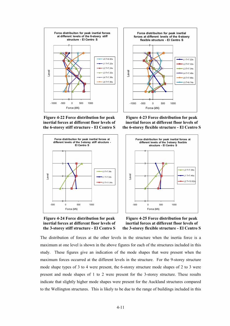
4�11

0

1

2

3

4

5

6

7

�1000 �500 0 500 1000

Level

Force (kN)

Force distribuiton for peak inertial forces at different levels of the 6�stoery stiff


L5 T=6.92s

L1 T=7.22s

L2 T=7.24s

L3 T=7.32s

L4 T=7.38s

L6 T=7.56s

0

1

2

3

4

5

6

7

�1000 �500 0 500 1000

Level

Force (kN)

Force distribuiton for peak inertial forces at different levels of the 6�stoery

flexible structure � El Centro S

L1 T=7.22s

L2 T=7.32s

L3 T=7.34s

L4 T=7.46s

L6 T=7.66s

L5 T=9.74s







0

1

2

3

4

�500 0 500 1000

Level

Force (kN)

Force distribuiton for peak inertial forces at different levels of the 3�storey stiff structure �

El Centro S

L3 T=7.38s

L1 T=7.52s

L2 T=11.04s

0

1

2

3

4

�500 0 500 1000

Level

Force (kN)

Force distribuiton for peak inertial forces at different levels of the 3�stoery flexible


L3 T=7.36s

L1 T=7.46s

L2 T=10.92s







The distribution of forces at the other levels in the structure when the inertia force is a

maximum at one level is shown in the above figures for each of the structures included in this

study. These figures give an indication of the mode shapes that were present when the

maximum forces occurred at the different levels in the structure. For the 9�storey structure

mode shape types of 3 to 4 were present, the 6�storey structure mode shapes of 2 to 3 were

present and mode shapes of 1 to 2 were present for the 3�storey structure. These results

indicate that slightly higher mode shapes were present for the Auckland structures compared

to the Wellington structures. This is likely to be due to the range of buildings included in this

4�12

study being in different period ranges of the response spectrum, which subsequently possibly

explains why the average maximum force distribution shapes differed between the structures

on different soil conditions.

4.3 Conclusions

This chapter investigated the distribution of forces which developed in the floor diaphragms

of moment resisting frame structures. The study investigated buildings of different heights (3,

6 and 9 stories), flexibilities (different fundamental elastic periods) and seismic locations

(Wellington with high seismicity and Auckland with low seismicity). The trends and

magnitudes of floor diaphragm forces obtained from this study were used to develop the floor

diaphragm force method which is described in Chapter 5.

The trends obtained from the results are listed in the following bullet points:

− The general vertical distribution of the average maximum inertial floor diaphragm

forces was different to that of the ESA method where forces reduce with reducing

levels of the building. The floor forces, for the 9�storey buildings, were found to be

large in the lower levels, decrease gradually to around 2/3rds of the height of the

building and then increase for the upper levels of the building;

− The average maximum inertial floor forces were not maximums at all levels for the

same time step during the time history analysis (did not occur simultaneously);

− The distribution of maximum average inertial forces was not predominantly from the

first mode response of the structure, it was typically from higher modes;

− The average maximum inertial forces at the lower floor levels of the 9�storey

Wellington building were related to dynamic mode shapes similar to mode 2 and

mode 3 for moment resisting frame buildings; for the 6�storey Wellington structure

mode 1 and 2 shapes were present; and for the 3�storey building the mode shapes

were found to be similar to the fundamental dynamic mode shape;

− The average maximum inertial forces at the lower floor levels of the 9�storey

Auckland building were related to dynamic mode shapes which were similar to mode

3 and mode 4; for the 6�storey Auckland structure mode shapes similar to 2 and 3;

and for the 3�storey building the mode shape were similar to modes 1 and 2;

− Higher mode shapes associated with the average maximum inertial floor forces were

observed for more flexible Auckland buildings compared to stiffer Wellington

structures.

4�13

4.4 References







Kermonde, L. (1992). Geology of the Auckland Urban Area. Lower Hutt, New Zealand,

Institute of Geological & Nuclear Sciences Limited.




New Zealand.

4�14

5�1

5 FLOOR DIAPHRAGM FORCE METHOD

5.1 Introduction

Simplistic floor diaphragm structural design methods play an important role in seismic

design. They enable quick efficient design to be carried out for regular structures and can

also be used to check results from more complex analytical models. Past researchers

(Bull (1997), Nakaki (2000) and Fleischman et al. (2002)) have indicated that some of the

currently available diaphragm design methods can give poor estimates of structural actions

compared with more sophisticated methods of analysis.

A new floor diaphragm design method, the pseudo Equivalent Static Analysis (pESA)

method, has been proposed in an attempt to capture more realistic design actions (Bull, 2003).

The pESA method is based on the concept of the ESA method, with some modifications to

account for the behaviour that the ESA approach fails to consider. These modifications

include; consideration of higher mode forces at the base of the structure and the amplification

of forces due to the over�strength actions which develop in the lateral force resisting systems.

To check the validity of the pESA method for determining floor diaphragm design actions,

the predictions from this approach were compared with corresponding values from time

history analyses. The magnitudes of inertial forces and displacements for each floor were of

particular concern. The numerical integration time history results used for this comparison

were from the studies that are described in Sections 3.4 and 4 for dual structures (walls and

frames) and moment resisting frame structures respectively. These time history results were

assumed to provide the most accurate estimate of inertial forces and displacements of the

structures.


5.2.1 Structural Design Methods

Various structural design methods, of differing degrees of complexity and accuracy, are used

to design floor diaphragms in structures. These include the; equivalent static analysis (ESA),

displacement based design, parts and components, modal analysis, pushover analysis and

elastic and inelastic time history analysis methods. Brief descriptions of these methods and

5�2

how they are used in the design of floor diaphragm design are provided in the following

sections.

5.2.1.1 Equivalent Static Analysis

The Equivalent Static Analysis (ESA) method is based on the assumption that the building

deforms in its fundamental translational free vibration mode and that essentially all the mass

contributes to this mode. On the basis of this assumption, the design base shear force is found

by multiplying the mass by a lateral force coefficient, which is determined from factors such

as: the seismic hazard factor, the soil class factor, the structural importance factor, the near

fault factor, the calculated or assumed fundamental period and the structural ductility factor

(Standards New Zealand, 2004a).

The individual equivalent static forces at each level are found by distributing the design base

shear force over the height of the structure. The New Zealand Structural Design Actions

Standard NZS1170.5 (Standards New Zealand, 2004a) 92% of the base shear is distributed

according to the maximum acceleration that the mass of each level would be expected to

sustain if the building remains in the elastic range. The accelerations at each level are

proportioned to the lateral deflections. For simplicity lateral deflections are assumed to be

proportioned to height above the base. The remaining 8% of the base shear is added to the

mass at the highest level to allow for higher elastic modes. For simplicity in the NZS1170.5,

the lateral deflection of the structure relative to the ground is assumed to increase linearly

with height.

Modal analyses of regular multi�storey buildings indicate that for taller buildings less of the

mass contributes to the first mode compared to shorter buildings. As a very high proportion

of the lateral deflection is accounted with the first mode, it follows that the ESA method,

which assumes 100% participation, overestimates lateral deflections when compared with

modal analyses. In NZS1170.5 a displacement modification factor is used to reduce the

discrepancy of displacements obtained from the ESA method and the modal analysis method.

Empirically derived coefficients are used to amplify lateral deflections to allow for the

anticipated level of inelastic deformation corresponding to the chosen structural ductility

factor used in assuming the design forces.

5.2.1.2 Modal Analysis

The modal response spectrum analysis is generally used when the higher mode affects are

considered to be significant. The property of orthogonallity of mode shapes is used to

5�3

transform the coupled equations of the Multi�Degrees�of�Freedom (MDOF) system, from the

equation of motion, to uncoupled Single Degree of Freedom (SDOF) systems. The SDOF

systems represent various modes of the structure. For each mode the: period, effective mass

and participation factors are found. These values are then used with the response spectra,

similar to the response spectra used for the ESA method, to determine the spectral

accelerations and displacements for each mode.

To find the design actions from a modal response spectrum analysis, it is necessary to

combine the actions from the different modes. As the peak mode values occur at different

times, the resultant actions cannot be found by a simple addition. Design values are

determined by methods such as the Sum Root Sum of the Squares (SRSS) or the Complete

Quadratic Combination (CQC) method. The number of mode shapes to be incorporated, to

determine the response of the structure, is determined by ensuring that in excess of 90% of the

total mass of the structure participates in the response of the structure, in the direction under

consideration. The deformations obtained from this method are increased to allow for

inelastic actions in a similar manner to that in the ESA method.

This method is based on linear elastic engineering theory, but has some assumptions which

simplify the method. However, the assumptions make it less accurate than more complicated

approaches such as time history analysis. The assumptions of this method include:

� The structure remains linearly elastic;

� Higher modes, which provide insignificant effective mass contribution, are assumed

to cause insignificant affects to the response of the structure;

� The use of the response spectra is appropriate for the design;

� The combination method used to determine the responses is practical.

The assumption that the system remains linearly elastic is questionable. The majority of

buildings today are designed to sustain some level of inelastic deformation to reduce the

costs.

Ignoring insignificant higher modes is a reasonable assumption. If a large proportion of the

effective mass is included in the response of the structure, then errors should be small due to

omission of higher modes with a small proportion of effective mass.

The use of the combination methods, the SRSS or the CQC, results in a loss of information,

such as the sign of the action. Consequences of this are:

− Design actions do not satisfy equilibrium;

5�4

− Design moments are not consistent with design shear, torsion or displacements.

The output values obtained from this method are maxima for each level of the structure and

they are not equivalent to a set of actions that occur simultaneously. Consequently, these

values should not be applied to the structure simultaneously, in an envelope fashion like the

ESA method, as the forces are not in equilibrium.

5.2.1.3 Parts and Components

The “Parts and Components” method is a force based design approach used for the design of

“parts” or “components” of a structure. This method was previously used to design the forces

which develop within floor diaphragms, as traditionally these elements were considered a part

(secondary in nature to the “primary” structure resisting lateral forces) and their influence on

the overall behaviour of the structure was neglected. The current New Zealand Structural

Design Actions Standard NZS1170.5:2004 (Standards New Zealand, 2004b) states that floor

diaphragms must be designed by considering the interaction of the floor with the structure as

a whole; therefore the “parts” method is no longer appropriate for the design of floor

diaphragms.

The Parts and Components method is carried out in a similar way to the ESA method. Firstly,

the elastic design spectrum for the part (or component) is determined with consideration of

the vertical location of the part within the structure and the fundamental period of the part.

The ductility, risk and weight of the part or component are taken account in determining the

design actions on the part. This method does not to consider force equilibrium, or the

interaction of the part or component with the remainder of the structural system.

5.2.1.4 Pushover Analyses

Pushover analyses are generally carried out by applying a monotonically increasing force

pattern to an elastic or inelastic responding structure. The lateral forces are increased until

either the total capacity of the structure is exceeded or a predetermined displacement of the

structure is reached. Damping of the structural response is not considered during pushover

analyses.

There are two difficulties with the general pushover method, they include: choosing an

appropriate load pattern to apply to the structure and determining an appropriate displacement

termination point. The results of general pushover analyses can be sensitive to the load

pattern used in the analysis and the termination point.

5�5

A variation of the general pushover is the adaptive pushover method. The phrase “adaptive”

is used because the parameters at each step of the analysis are updated. This includes

parameters such as lateral force distribution, period and displacement of the structure.

The adaptive pushover method was developed to avoid the uncertainties surrounding the

pattern of forces to be applied to the structure. With this approach, the loading pattern adjusts

itself to the level of deformation of the structure. The loading pattern is dependent on the

mass, the equivalent frequency and displaced shape of the structure.

Comparisons of predictions from pushover and time history analyses show that the pushover

values tend to under�estimate inter�storey drifts in the lower levels of buildings. This aspect

is particularly significant in multi�storey moment resisting frame buildings. The

discrepancies arise as pushover analyses fail to allow for higher mode affects associated with

the formation of plastic hinges in the lower reaches of buildings (Fenwick and Davidson

(1991),(1997)).

5.2.1.5 Time History Analysis

Numerical integration non�linear time history analysis (THA) is a complex and time

consuming analytical method for determining the seismic response of structures. This method

appears to be the most comprehensive technique as it makes allowance for the designed

strength of plastic hinge zones and the hysteretic behaviour of these zones. However, due to

the sensitivity of response to individual seismic ground motions, a number of different

analyses are required, using different ground motions, to enable a safe design to be made.

Time history analyses use numerical integration to solve the response of a multi�degree of

freedom structure. It can directly modify the stiffness of the elements and joints based on the

deformation states. The equation of motion incorporates the mass, damping and stiffness of

the structure and the dynamic loading from the earthquake ground motion.

The design process requires a vast range of information for the elements of a structure such

as: geometries, strength, yield and hysteretic properties. The time history records, which are

applied when using THA, need to be carefully chosen to ensure they are representative of the

likely ground motion for the location of structure of interest. For example, the records chosen

should match the typical type of ground rupture, duration of shaking, frequency content and

other effects associated with the site. To ensure the time history records are of reasonable

magnitude, they are generally required to be scaled to match a response spectrum for the site.

5�6

5.2.2 Design Procedures: Standards and Codes

5.2.2.1 NZS1170.5

The New Zealand Structural Design Actions Standard NZS1170.5:2004 (Standards New

Zealand, 2004a) provides restrictions on the use of some analysis methods. The ESA method

may be employed when at least one of the following criteria is satisfied:

� The height between the base and the top of the structure is less than 10m;

� The largest translational period calculated is less than 0.4s;

� The structure is not classified as irregular by the Standard and the largest translational

period is less than 2.0s.

For structures which do not met the criteria for the ESA method, a two dimensional (2D)

modal response spectrum method may be employed if the structure is not classified as

torsionally sensitive, as per (Standards New Zealand, 2004a). If the structure is classified as

torsionally sensitive either a three dimensional modal response spectrum or a time history

analysis should be employed. Generally, time history analyses are made for major structures

to check that structures, designed on the basis of the modal response spectrum approach, are

adequate.

The New Zealand Structural Design Actions Standard provides requirements on how floor

diaphragms should be analysed. These require buildings over 15m in height, which are

classified as irregular, to be analysed with either the three dimensional modal response

spectrum method or by three dimensional THA and also consideration is given to the of

flexibility diaphragms for diaphragms which are assessed to be flexible.

5.2.2.2 FEMA450

The American Seismic Design Standard FEMA450 (National Earthquake Hazards Reduction

Program (U.S.) et al., 2004) is similar to other design codes in that it imposes restrictions on

the use of some design methods for more complicated types of structures. The use of all

analytical methods including: the ESA, modal response spectrum procedure, elastic and

inelastic time history analysis methods, are permitted for both regular and irregular structures

which have a low associated seismic hazard level. Further, a structure which is of light�

framed construction, limited irregularities and has a fundamental period which is less than 3.5

times Ts, where Ts is the period where the constant velocity section of the response spectrum

starts, may also be designed with all of these analyses methods. All other structures are not

permitted to be designed using the ESA method and other, more complex, approaches are

required.

5�7

In the USA, the design method for diaphragms depends on the seismic design category and

the structural characteristics of the building (seismic force resisting system, fundamental

period of vibration and the configuration of the structure). The seismic design category is

based on the importance of the structure and the seismicity of the region. Seismic design

category A is the least hazardous and seismic design category F is the most hazardous.

For seismic design category A, the lateral force applied to the diaphragms shall be calculated

from Equation 5�1.

xx wF 01.0= Equation 501

Where Fx is the design lateral force and wx is the portion of total seismic weight, located at

level x.

For seismic category B, a minimum force that should be used, applied to the diaphragm, is

equal to 20% of the short period design spectral response acceleration, SDS, multiplied by the

weight of the floor, together with the weight of other attached elements plus the portion of

base shear force at the level which is to be resisted by the seismic force resisting system.

For seismic design category C, the structural analysis methods, which are allowed to be used

to determine the design forces, are the same as those in seismic category B with some

additional restrictions.

For seismic design category D, E and F, diaphragms shall be designed to resist the forces

obtained from proportioning the values from the ESA method to the relative weight of the

floor diaphragm, as indicated by Equation 5�2.

pxn

xi

i

n

xi

i

px w

w

F

F

∑

∑

=

== Equation 502

Where wi is the weight associated with level i, Fi is the lateral force at level i, n represents the

number of levels and wpx is the weight associated with the diaphragm of interest.

In the situation where vertical or plan irregularity may exist, the design forces are increased

by an adjustment factor which gives an additional 25% for connections of diaphragms to

5�8

vertical resisting system elements. Criteria for when diaphragm flexibility should be

considered in a design are also provided.

5.2.2.3 Eurocode 8

In Eurocode 8 (British Standards Institution., 2005) the design criterion for floor diaphragms

is similar to that provided in the New Zealand Structural Design Actions Standard. The ESA

method may be used for structures where higher modes do not significantly affect the

structural response and the structure meets the regularity requirements. Modal response

spectrum analyses are to be carried out when the ESA method does not satisfy the criteria

outlined above. Structures which do not meet these criteria were required to be designed

using modal response spectrum 3�dimensional analysis.

Structural regularity is considered in Eurocode 8 (2004) by considering the: symmetry,

stiffness and mass distribution of the building, set backs in the floor, stiffness and the

slenderness of the floor diaphragm. If the structure is found to be irregular, a reduction factor

of 0.8 is applied to the behaviour factor (the behaviour factor is an approximation of the ratio

of the seismic force that is expected to occur in the structure if the structure was to remain

elastic and the seismic force that can be used in design) and limits are imposed on the method

of analysis that can be used. This factor results in increasing the strength of the structure by

25% and it is similar to the adjustment factor that is used in FEMA450.

5.2.3 Bull (2003)

Bull (2003) suggested that a type of pseudo�equivalent static analysis (pESA) method could

be used to find floor diaphragm forces. This approach was suggested as an alternative method

to the “Parts and Component” and the ESA methods. The “Parts and Components” approach

vastly over predicts the forces and the ESA method under predicts the forces at the lower

levels of the structure. Bull (2003) described the pESA method as one that is based on the

application of a set of static forces, which is static method which is similar to the ESA

method, but it accounts for over�strength of the structure due to the inelastic response of the

lateral force resisting system.

The pESA method was visualised as an equivalent type of method where equilibrium was

maintained in the system allowing the force paths to be tracked through the floor diaphragm

to different parts of the lateral force resisting system. The method was also envisaged to

account for both the affects of transfer and inertial forces.

5�9

5.2.4 Rodriguez et al. (2000)

Rodriguez et al. (2000) carried out an analytical investigation on earthquake induced

horizontal floor accelerations that developed in regular buidings with rigid diaprhagms. A

new method, referred to as the first mode reduced method, which estimates the accelerations

which develop in floor diaphagms was proposed from their work.

The first mode reduced method determines the absolute floor accelerations by the use of

Equation 5�3. It is based on findings from a parametric analysis that was carried out on a

twelve�storey cantilever wall building that was designed with a structural ductility of 5. The

parametric study was carried out using non�linear time history analysis. The findings from

this parametric study were:

− The maximum floor amplification occurs when the building responds elastically;

− The floor amplification tends to diminish as the ductility demand increases.

The absolute floor acceleration, Aq

n, is given by Equation 5�3.

q

qqq

nq

q

nR

TSaA

),( ξΦΓ=

Equation 503

Where Гq is the participation factor for mode q, Φq

n is the mode shape for mode q at level n,

Sa is the spectral acceleration, Tq is the period of free vibration associated with mode q, ξq is

the damping ratio for mode q and Rq is the reduction factor to account for the ductility of the

system.

A simplification of this method was made as a parametric study found that higher modes are

not significantly affected by the ductility of the system. This allowed Rq, for modes greater

than 1, to equal 1. Additional assumptions were made to allow it to be used with a generic

design spectrum. These included:

− Assume all modes of free vibration have the same damping ratios, which allows the

spectral acceleration terms to be obtained from the same design spectra;

− All natural periods of free vibration corresponding to the high translational modes are

associated with the maximum spectral ordinate.

The simplified equation, based on these assumptions, is shown in Equation 5�4 and how this

correlates to the horizontal design force for a floor is given in Equation 5�5.

5�10

[ ]2

2

1

1

1 )ln(7.0)1,( hohpm CnTCR

nC +

=

Equation 504

ppippph WZCRSF = Equation 505

Where n1, is a first mode contribution coefficient, R1, a ductility factor (�/2 or 1, the greater),

Ch(T,1), is the horizontal seismic coefficient, Cho, is the peak ground acceleration divided by

the acceleration of the gravity defined in the basic hazard acceleration design spectra, Sp is

the structural performance factor, Rp is the risk factor for the part, Z is the seismic zone factor,

Cpi is the basic design coefficient at the intermediate level between the base and the level

corresponding to the uppermost principle seismic weight and Wp is the weight of the part.

5.3 Motivation

The Equivalent Static Analysis (ESA) method, which is commonly used for seismic design of

structures, determines the forces for the lateral force resisting system of the structure.

However, this approach does not adequately account for the forces which develop in floor

diaphragms. These forces are under predicted due to over�strength affects and both higher

elastic and inelastic mode actions.

Various researchers, as described in Section 5.2.2.1, have indicated that the ESA method

poorly predicts the forces which develop in the lower floors of structures. Findings from both

the dual structures study and the moment resisting frame study (described in Chapter 3 and 4)

indicate diaphragm forces are higher than the forces predicted by the ESA due to higher mode

effects.

Inelastic time history analysis (THA) currently provides the most accurate estimate of the

behaviour of a structure in response to earthquake actions. This method requires a

considerable amount of information about the details of the structure and a substantial amount

of time to carry out the required analyses. Static design approaches provide a simpler,

quicker option for regular structures which avoid the sensitivity of the predicted actions to the

choice of earthquake records and the hysteretic response relationships assumed for plastic

regions, associated with THA procedures.

The first mode reduced method, proposed by Rodriguez et al. (2000), provides an approach

with a level of complexity that lies between the ESA and inelastic time history analysis

5�11

methods. The forces are obtained by using the philosophy of the “parts” method. Floor

diaphragms interact with the lateral force resisting elements in the structure and consequently

should be designed alongside the whole structure rather separately. Therefore applicability of

the first mode reduced method is in doubt.

Floor diaphragms were previously constructed as cast insitu elements, but are now

constructed using precast flooring systems with a cast topping to increase the speed of

construction. Precast flooring systems do not provide as robust a system compared to cast

in�situ floor system due to the increased number of connections involved with precast

construction. The lack of robustness of precast flooring systems provides further motivation

to ensure that better methods are used to estimate the forces which develop in floor

diaphragms.

This review of the literature indicates that there is currently no existing simple design

approach based on the applied static forces that gives a realistic estimate of the design floor

diaphragm forces. To fill this gap, the suggestions made by Bull (2003) regarding the general

concept of the pseudo�Equivalent Static Design method have been used, and extended, with

use of results from earlier sections of this study, to develop a simple desktop floor diaphragm

design method. Descriptions of this proposed method are provided in the following sections.

5.4 The pseudo0Equivalent Static Analysis (pESA) method

The proposed pESA desktop method may be used to determine the design actions in floors,

which act as diaphragms in multi�storey buildings with beam sway mechanisms. The inertial

forces are determined by carrying out the pESA method. The details of this approach are

given in Sections 5.4.2 and 5.4.3. The transfer forces are obtained from statically applying

the inertial forces, obtained from the pESA method, to an elastic structure. These forces were

found to provide about the right displacements and therefore magnitudes of transfer forces.

Comparisons of the estimates from total floor diaphragm forces from different static

diaphragm design methods and the time history method are provided in Section 5.5. Findings

from the literature, and past researchers, which were used as part of the basis for this method

are provide in Section 5.4.1.

The forces obtained from this method represent the inertial forces which develop in the floor

diaphragm. The compatibility transfer forces, which are discussed in Chapter 2 and 3, are

also considered by ensuring that this approach provides an adequate prediction of the

displacements, which control transfer forces, of the structure.

5�12

5.4.1 Basis of pESA Method

Reviews of the literature and findings from former Chapters of this research have provided

information with regard to developing a possible floor diaphragm design method. A summary

of these findings, which were used in the development of this method, are provided in the

following bullet points:

− Transfer forces have a significant contribution to the total magnitude of floor

diaphragm forces (Chapter 2, Chapter 3, Beyer (2005));

− Transfer forces were found to be controlled by the displacements of the structure

(Chapter 2 and 3);

− Transfer forces were found to be affected by the changes of displacement patterns due

to the development of localised plastic hinge zones in the structure (Chapter 2.3.3.2).

The affects of localised plastic hinge zones on the distributions of transfer forces were

captured by determining the trends and magnitudes of transfer forces for a range of

earthquake records;

− Inertial forces were found to be controlled by higher modes. Larger inertial forces

compared to actions from Equivalent Static Analysis (ESA) methods develop in the

lower levels of buildings (Chapter 3, 4, Bull (1997), Rodriguez et al. (2002) and

Fleischman (2002));

− Both transfer forces and inertial forces were found to occur simultaneously (Chapter 2

and 3);

− Maximum floor diaphragm inertial and transfer forces were found to occur at

different times. The total floor diaphragm forces were determined by the maximum

combination of inertial and transfer forces and not the maximums of the components

(Chapter 2 and 3).

Descriptions of how each of these findings was incorporated into the pESA method are

provided in the following Sections.

5.4.2 Overview of Method

The pESA and ESA methods are similar in that lateral forces, which represent the seismic

actions at each level of the structure, are given by the product of the seismic weight of the

level times a lateral force coefficient for that level.

5�13

Lateral force

Lev

el Upper region:

pESA1 = Ø .ESAo.b

Lower region:pESA2 L

fc

pESA envelopeESA envelope

Figure 501 Schematic of the inertial forces from pESA method

The distribution of the pESA lateral force coefficients on a multi�storey building are

illustrated in Figure 5�1. As illustrated in the figure, there are two sets of lateral force

coefficients. In the upper region, denoted by pESA1, the lateral forces are equal to the ESA

forces multiplied by an over�strength factor, Øob, see Section 5.4.2.1. In the lower region,

pESA2, the lateral coefficient is constant, see Section 5.4.2.2.

5.4.2.1 The Upper Region

The upper region pESA forces are found by scaling the ESA forces by an over�strength factor,

Øob and they are applied to the centre of mass at each level. The ESA forces correspond to

the design action values action at the centre of mass of each level.

The over�strength factor, Øob, is obtained by locating the plastic hinge regions in the building

and either:

1. The over�strength of each potential plastic hinge is formed and these values are used

to calculate the base shear; or

2. The practical strength of the plastic hinges is found together with an appropriate

strain hardening rate, and then a pushover analysis is performed. The pushover

analysis is continued until the lateral displacement at the top of the building is equal

to 3.75% of the height. This drift is deemed to be the maximum credible drift

expected in a building designed to the New Zealand Structural Design Actions

Standard NZS1170.5 (Standards New Zealand, 2004a).

5�14

The over�strength factor, Øob, is equal to the base shear force given by either 1 or 2 above

divided by the design action base shear from the ESA method. The commentary of the New

Zealand Structural Design Actions Standard (Standards New Zealand, 2004b) indicates that

the minimum building over�strength factor should be in the range of 2�2.5.

5.4.2.2 The Lower Region

Past research, together with the results from Chapters 3 and 4, has indicated that inelastic

higher modes contribute to the forces which develop in floor diaphragms. These additional

forces have been incorporated by the pESA method by the forces which are applied to the

lower levels indicated by the “lower region” in Figure 5�1. The lateral forces in the lower

region are found by multiplying the mass at each level by a lateral force coefficient, which is

the same for all levels in the lower region. The region is bounded by the bottom level of the

structure and the level at which the Lfc value equal to the Øob.ESA value. The Lfc value

represents ground motion and higher mode effects that are not captured by the ESA or the

modal analysis response spectrum methods.

Period

Design action spectrum, C (T )h 1

Modified spectrum, C (T )hmod 1

T1

Sp

ectr

um

va

lue

Figure 502 Design action spectrum

The modified spectral shape factor, Chmod(T) allows the influence of higher modes actions on

the lower levels of the building to be represented in analyses. The lateral force coefficient,

Lfc, is found from a modified form of the inelastic design response spectrum (Figure 5�2).

The inelastic design response spectrum, Cd(T1), is found from the New Zealand Structural

Design Actions Standard NZS1170.5 or other appropriate earthquake action code. For the

New Zealand Structural Design Actions Standard, the design spectrum is given by

Equation 5�6.

5�15

Cd(T1) = Ch(T).Z.R.N(T,D).Sp/kI Equation 506

Where Ch(T) is the spectral shape factor for the subsoil type, Z is the seismic zone factor, R is

the return factor, N(T,D) is the near fault factor, Sp is the structural performance factor and k�

is the structural ductility factor.

The factor used to determine the lower floor diaphragm forces, Lfc, is obtained by using

Equation 5�7. This factor is obtained from the product of: the modified spectral shape factor,

Chmod(T), a seismic zone factor, Z, return period factor, R, structural performance factor, Sp,

over�strength factor of the lateral force resisting system, Øob, and the structural ductility

factor, k�. The Chmod(T) is obtained from the values provided in Section 5.4.3. The over�

strength factor of the lateral force resisting system was included in this equation to adjust the

magnitude of forces which developed in the lateral force resisting system to the magnitude of

over�strength actions. The other factors represent the affects of the: period of the structure,

category of the seismic hazard, importance of the structure and performance of the structure.

Lfc(T1) = Chmod(T).Z.R.Sp.Øob/KI Equation 507

5.4.3 Modified Spectral Shape Factor (Chmod(T1))

To calculate the value of, Lfc, the design spectra shape factor is modified, Chmod(T1). This

change is made to allow for higher (elastic and inelastic) mode effects in the lower levels of

buildings and peak ground accelerations to be represented in analyses. Results from

Chapters 3 and 4 and past researchers (Bull (1997), Rodriguez et al. (2002) and Fleischman

(2002)) indicated that higher modes influences the inertial forces in the floor diaphragms at

lower levels of buildings. Comparisons with ESA methods indicated that the floor diaphragm

forces are underestimated in these levels. This Chmod(T1) factor has been introduced to

account for this underestimation of forces.

This factor was based on the Ch(T) value from the New Zealand Structural Design Actions

Standard (Standards New Zealand, 2004a). The factor was based on this value to capture the

variation of floor diaphragm forces for different soil conditions including soil type A, B, C

and D as defined in New Zealand Structural Design Actions Standard (Standards New

Zealand, 2004a) and variation in different fundamental elastic periods of the buildings. The

results presented in Chapters 3 and 4 for dual frame�to�wall and moment resisting frame

buildings indicated that the type of soil has an affect on the magnitude of total (transfer and

inertial) floor diaphragm forces. The results from Section 2.3.4 and Chapters 3 and 4 also

5�16

indicated that the results are significantly affected by the elastic fundamental period of the

structure.

Calibration of the modified spectral shape factors was carried out by using the average peak

time history inertial force results, for the dual structures which were presented in Chapter 3,

and for the moment resisting frame structures presented in Chapter 4. Comparisons are made

between the pESA values, the calibrated (modified) spectral shape factor curves, Chmod(T1)

and the spectral shape factor curves according to the New Zealand Structural Design Actions

Standard (Standards New Zealand, 2004a), NZS1170.5Ch(T). These comparisons are

provided in Sections 5.4.3.1 and 5.4.3.2 for moment resisting frames and dual structures,

respectively; the results are for a range of soil types.

The calibrated values were based on 1 in 10 (90th percentile) pESA floor force results being

below the time history values. The reason behind choosing the 90th percentile was based on:

the ability of the structure to redistribute internal forces and the material strengths were based

on nominal strength values. Therefore, it was thought that a less stringent value, compared to

the 95th percentile which is used for nominal material strengths in the New Zealand Concrete

Structures Standard (Standards New Zealand, 2006), would be acceptable.

In the following development of the Chmod(T1) design curves, there are cases where limited

data points are available. Past results, presented in Chapters 3 and 4, indicated that higher

mode effects are less prevalent for shorter period structures. Therefore, the higher mode

acceleration factors should reduce with smaller elastic fundamental periods, T1. The spectral

shape factor curves according to the New Zealand Structural Design Actions Standard

(Standards New Zealand, 2004a), NZS1170.5Ch(T), represents the influence of elastic

fundamental period of the structure and the affects due to the soil conditions. The difference

of the gradient between the NZS1170.5Ch(T) curve and the Chmod(T1) curve is related to higher

mode affects (the magnitudes of these curves differ due to the different uses for these two

values). For shorter period structures the gradient of the Chmod(T1) curve reduces compared to

the gradient of the NZS1170.5Ch(T) curve due to reducing higher mode affects (the opposite

for longer period structures) as shown in the comparisons between the curves in Sections

5.4.3.1 and 5.4.3.2. For the cases where limited data was available and the Chmod(T1) curve

was shown to be reducing with reducing fundamental period relative to the NZS1170.5Ch(T)

curve, the modified spectral shape factor, Chmod(T1), curve was kept at a constant distance

(similar gradient) from the NZS1170.5Ch(T) curve. This gives conservative results as it does

not represent the reduction of the Chmod(T1) value due to reducing higher mode affects for

buildings with reducing elastic fundamental periods for this range of buildings.

5�17

5.4.3.1 Moment Resisting Frame Structures

Soil category A/B:

0.0

0.5

1.0

1.5

2.0

2.5

3.0

3.5

0.3 0.6 0.9 1.2 1.5

Sp

ect

ral s

ha

pe

fa

cto

r C

h(T

)

Period (s)

Modified spectral shape values for soil class

A/B with period between T1=0.3 to T1=1.5s

pESA Ch(T)

Modified

Ch(T)

NZS1170.5

Ch(T)

Figure 503 Modified spectral shape values for soil class A/B with period between T1=0.3

to T1=1.5s

Figure 5�3 provides a comparison between the calibrated data indicated in this figure by,

pESA Ch(T1), the proposed modified spectral shape factor curve for determining the higher

mode forces, indicated by Modified Chmod(T1), and the spectral shape factor curve from the

New Zealand Structural Design Actions Standard, NZS1170.5 Ch(T1).

The calibrated data shown in this figure is predicted reasonably well by the proposed

modified spectral shape factor curve for structures with fundamental translational periods

between 0.5s and 1.5s. The data points represent a reasonable spread of structures with

different fundamental periods. The comparison over the range of 0.3s to 0.5s is poor. Over

this range, the values for the suggested modified spectral shape factor was kept at a constant

distance from the modified spectral shape factor values presented in the New Zealand

Structural Design Actions Standards.

5�18

0.0

0.5

1.0

1.5

2.0

2.5

3.0

3.5

1.5 1.8 2.1 2.4 2.7 3

Sp

ect

ral s

ha

pe

fa

cto

r (C

h(T

))

Period (s)

Modified spectral shape values for soil class A/B

with period between T1=1.5 to T1=3.0s

pESA Ch(T)

Modified

Ch(T)

NZS1170.5

Ch(T)


to T1=3.0s

Figure 5�4 shows the comparison of calibrated data to the proposed modified spectral shape

curve for structures with periods from 1.5 to 3.0s. This figure indicates that a constant line

provides a reasonable correlation to the calibrated data. Only 3�data points were available

from the results for this comparison, this does not provide enough information to prudently

determine modified spectral shape factors for this region of the curve. The results for similar

structures on different soil conditions indicate that over this region a straight line was

appropriate in this region. As a result of this, it is recommended that a straight line be used

for this region. The values for the curves shown in Figure 5�3 and Figure 5�4 are the same at

T1=1.5s.

Structures which have fundamental periods in the constant acceleration range, T1=0s to 0.3s,

have not been included in this study. Multi�storey buildings are typically more flexible than

this. Higher mode effects were found in the above results to be less significant for shorter

period structures. Therefore, the modified spectral shape factor is assumed to be constant

between T1=0 to T1=0.3s. Using this value should provide conservative results as the higher

mode effects are expected to decrease for shorter period structures.

Structures with fundamental periods of greater than 3s were not included in this study. They

inherently posses complex dynamic behaviour and therefore were not included in these

comparisons. The design of the floors for these flexible buildings should be carried out by

more comprehensive analyses methods than the proposed pESA method.

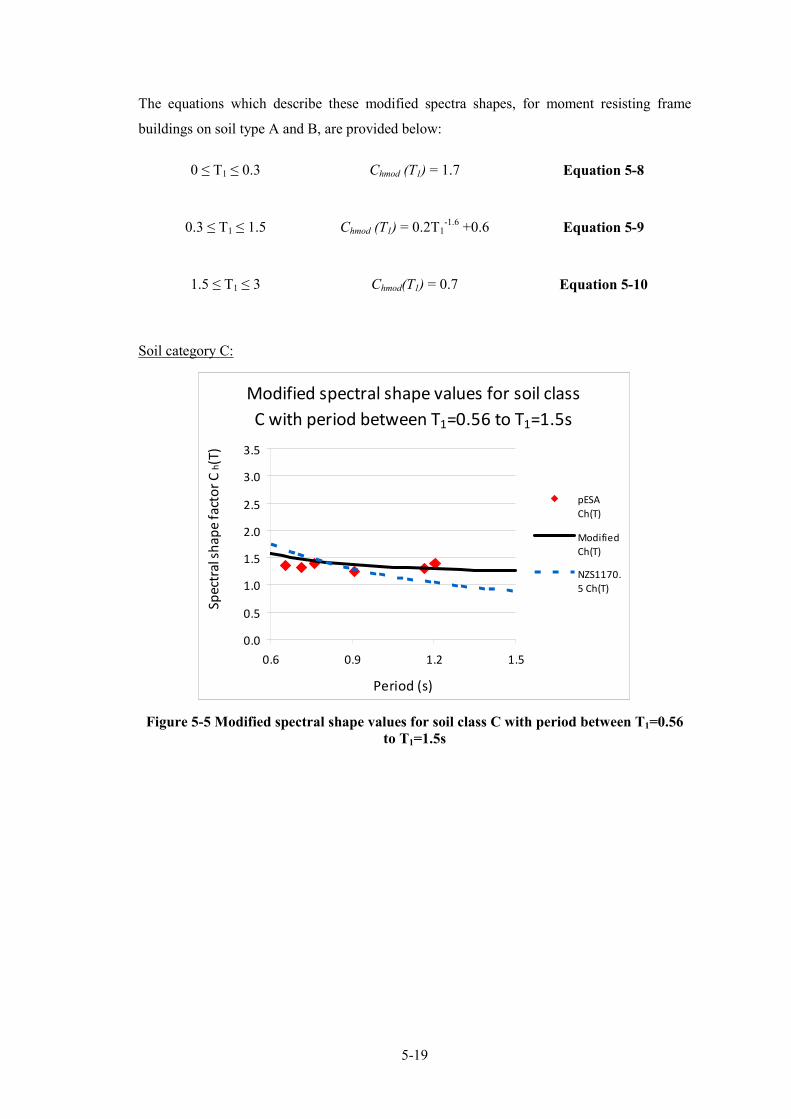
5�19

The equations which describe these modified spectra shapes, for moment resisting frame

buildings on soil type A and B, are provided below:

0 ≤ T1 ≤ 0.3 Chmod (T1) = 1.7 Equation 508

0.3 ≤ T1 ≤ 1.5 Chmod (T1) = 0.2T1�1.6

+0.6 Equation 509

1.5 ≤ T1 ≤ 3 Chmod(T1) = 0.7 Equation 5010

Soil category C:


C with period between T1=0.56 to T1=1.5s

0.0

0.5

1.0

1.5

2.0

2.5

3.0

3.5

0.6 0.9 1.2 1.5

Period (s)

Sp

ect

ral s

ha

pe

fa

cto

r C

h(T

)

pESA

Ch(T)

Modified

Ch(T)

NZS1170.

5 Ch(T)

Figure 505 Modified spectral shape values for soil class C with period between T1=0.56

to T1=1.5s

5�20


C with period between T1=1.5 to T1=3.0s

0.0

0.5

1.0

1.5

2.0

2.5

3.0

3.5

1.5 1.8 2.1 2.4 2.7 3

Period (s)

Sp

ect

ral s

ha

pe

fa

cto

r (C

h(T

))

pESA Ch(T)

Modified

Ch(T)

NZS1170.5

Ch(T)

Figure 506 Modified spectral shape values for soil class C with period between T1=1.5 to

T1=3.0s

The comparisons shown in Figure 5�5 and Figure 5�6 indicate that the calibrated data is

predicted reasonably well by the proposed modified spectral shape factor curves. Limited

data was available for structures with fundamental periods between 1.2 and 1.5s. The results

shown in Figure 5�6 indicate that a constant line is adequate to predict the values between 1.5

and 3.0s therefore a constant value between 1.2 and 1.5s should be acceptable.

The equations which describe these spectra shapes, for moment resisting frame buildings on

soil type C, are provided below:

0 ≤ T1 ≤ 0.56 Chmod(T1) = 1.6 Equation 5011

0.56 ≤ T1 ≤ 1.5 Chmod(T1) = 0.2T1�1.8

+1.2 Equation 5012


5�21

Soil category D:

Modified spectral shape values for soil class D


0.0

0.5

1.0

1.5

2.0

2.5

3.0

3.5

0.3 0.6 0.9 1.2 1.5

Period (s)

Sp

ect

ral s

ha

pe

fa

cto

r C

h(T

)

pESA Ch(T)

M odified

Ch(T)

NZS1170.5

Ch(T)

Figure 507 Modified spectral shape values for soil class D with period between T1=0.3 to

T1=1.5s

Figure 5�7 provides a comparison between the calibrated data, pESA Ch(T1), the proposed

modified spectral shape factor curve, Modified Chmod(T1), and the spectral shape factor curve

from the New Zealand Structural Design Actions Standard, NZS1170.5 Ch(T1).

The calibrated data shown in this figure is predicted reasonably well by the proposed

modified spectral shape factor curve for structures with fundamental translational periods, T1,

between 0.7s and 1.5s. No data was obtained for structures with periods between of less than

0.7s. The modified spectral shape factor curve, for the structures with fundamental periods

between 0.4s and 0.7s, was assumed to be at a constant distance below the New Zealand

Structural Design Actions Standard spectral shape factor curve to give conservative results.

5�22



0.0

0.5

1.0

1.5

2.0

2.5

3.0

3.5

1.5 1.8 2.1 2.4 2.7 3

Period (s)

Sp

ect

ral s

ha

pe

fa

cto

r (C

h(T

))

pESA Ch(T)

M odified

Ch(T)

NZS1170.5

Ch(T)

Figure 508 Modified spectral shape values for soil class D with period between T1=1.5 to

T1=3.0s

Figure 5�8 provides comparisons of the results for structures on soil type D with a

fundamental period between 1.5s to 3.0s. This figure indicates that a constant line, for the

modified spectral shape value, provides a reasonable comparison to the calibrated results.

Structures with a fundamental period in the range, T1=0 to 0.4s, were not included in this

study. For structures with these fundamental periods it is suggested, as above, that a constant

value equal to the modified spectral shape factor at 0.4s should be used.

The equations which describe these spectra shapes, for moment resisting frame buildings on

soil type D, are provided below:

0 ≤ T1 ≤ 0.3 Chmod (T1) = 2.1 Equation 5014

0.3 ≤ T1 ≤ 1.5 Chmod (T1) = 0.3T1�1.4

+0.5 Equation 5015


5�23

5.4.3.2 Dual System Structure

Soil category A/B:

0.0

0.5

1.0

1.5

2.0

2.5

3.0

3.5

0.3 0.6 0.9 1.2 1.5

Sp

ect

ral s

ha

pe

fa

cto

r C

h(T

)

Period (s)

Modified spectral shape values for soil class A/B


pESA Ch(T)

Modified

Ch(T)

NZS1170.5

Ch(T)


to T1=1.5s

Figure 5�9 provides a comparison between the calibrated data (pESA Ch(T1)), the proposed

modified spectral shape factor curve (Modified Chmod(T1)) and the spectral shape factor curve

from the New Zealand Structural Design Actions Standard (NZS1170.5 Ch(T1)) for soil types

A/B. The proposed modified spectral shape factor curve is shown to provide a reasonable

approximation to the calibrated pESA data results.

No data was available for structures with fundamental periods of less than 0.3s and greater

than 1.5s. For structures with fundamental period of less than 0.3s it is suggested that a

constant value of Chmod(0.3) is used. For structures with periods greater than 1.5s, additional

studies would be required for the use of this method. Frame�to�wall structures, on a rigid

foundation with a fundamental period greater than 1.5s are not likely to be greater than 9�

storeys high, and therefore not commonly constructed in New Zealand.

The equations which describe these spectra shapes, for dual buildings on soil type A and B,

are provided below:


5�24

0.3 ≤ T1 ≤ 1.5 Chmod(T1) = 0.1T1�1.8

+0.7 Equation 5018

Soil category C:

Modified spectral shape values for soil class C


0.0

0.5

1.0

1.5

2.0

2.5

3.0

3.5

0.5 0.7 0.9 1.1 1.3 1.5

Period (s)

Sp

ect

ral s

ha

pe

fa

cto

r C

h(T

)

pESA Ch(T)

Modified

Ch(T)

NZS1170.5

Ch(T)

Figure 5010 Modified spectral shape values for soil class C with period between T1=0.5

to T1=1.5s

This figure provides a reasonable comparison between the calibrated pESA values from time

history analysis and the suggested modified pESA method spectral shape factor for structures

with periods between 0.5s to 1.0s. No data was available for structures with fundamental

periods of greater than 1.0s. It is expected, that the Chmod(T1) values would be larger for

buildings with fundamental periods of greater than 1.0 compared to the values found for

buildings with fundamental periods of less than 1.0 due to the increase in higher mode affects.

The increase of Chmod(T1) values is unknown and therefore no Chmod(T1) values have been

provided for this range. Subsequently, this method should not be used for dual structures with

fundamental periods greater than this period.

The equations which describe these spectra shapes, for dual buildings on soil type C, are

provided below:


0.56 ≤ T1 ≤ 1.0 Chmod(T1) = 0.2T1�2.3

+1.9 Equation 5020

5�25

Soil Category D:



0.0

0.5

1.0

1.5

2.0

2.5

3.0

3.5

0.3 0.6 0.9 1.2 1.5

Period (s)

Sp

ect

ral s

ha

pe

fa

cto

r C

h(T

)

pESA Ch(T)

Modified

Ch(T)

NZS1170.5

Ch(T)

Figure 5011 Modified spectral shape values for soil class D with period between T1=0.3

to T1=1.5s

Figure 5�11 provides a comparisons between the calibrated data (pESA Ch(T1)), the proposed

modified spectral shape factor curve (Modified Chmod(T1)) and the spectral shape factor curve

from the New Zealand Structural Design Actions Standard (NZS1170.5 Ch(T1)) for soil

type D.

For structures with fundamental periods between 0.3 and 1.5s, the proposed modified spectral

shape factor curve is shown to provide a reasonable approximation to the calibrated results

from time history analysis. For these results, no data points were available for structures with

fundamental periods of less than 0.7s. For reasons previously discussed, the higher mode

acceleration factors were kept at a constant distance to respect to the spectral shape factors

from the New Zealand Structural Design Actions Standard.

No data was available for structures with fundamental periods of less than 0.3s. As

previously described the constant value at Chmod(0.3) will be used. Three data points were

available for structures with fundamental periods greater than 1.5s; these were all

concentrated with fundamental periods of around 1.8s. The available data was too limited to

provide prudent suggestions for the use of this method over this data range; further research is

suggested for this area. Structures in this range of flexibility are likely to exhibit higher mode

affects (as indicated in the results presented in Section 3.4.1.2) which could influence the

Chmod factor. Therefore structures in this range should not be designed using this method.

5�26

The equations which describe these spectra shapes, for dual buildings on soil type D, are

provided below:


0.3 ≤ T1 ≤ 1.5 Chmod(T1) = 0.1T1�1.8

+1.4 Equation 5022

5.5 Comparison of Diaphragm Design Methods to Time

History Results

Comparisons were made between the average maximum time history total floor forces for the

seismic frame structures, presented in Chapter 4, and the dual structures, presented in Chapter

3, to corresponding values predicted by different diaphragm design methods. The time

history results were assumed to provide the most accurate estimate of the response of the

structure. The diaphragm design methods which were used in this comparison were: the ESA,

the pESA and the Parts and Components methods.

The fundamental translational periods used to determine the set of static forces for the

diaphragm design methods are reported in Chapter 3 and Chapter 4 for the dual buildings and

the seismic frame buildings, respectively.

The over�strength factors for the lateral force resisting systems of these structures, which are

required for the pESA method, were calculated by carrying out pushover analyses. The Parts

and Components method was carried out according to the New Zealand Structural Design

Actions Standard (Standards New Zealand, 2004a).

5.5.1 Moment Resisting Frame Structures

Comparisons between the average maximum floor diaphragm total force results from time

history analyses and the different floor diaphragm design methods, for the structures in the

moment resisting frames, are provided in the following figures. Results are shown for the 3, 6

and 9�storey buildings that were proportioned for soil type D for both the Auckland and the

Wellington regions of New Zealand. Results are provided for each height, and flexibility;

including both stiff and flexible buildings, as categorised in Section 2.3.4. Results for other

soil types are shown in Appendix C.1.1.

5�27

For the following figures, P+C refers to parts and components, ESA refers to the Equivalent

Static Analysis method multiplied by over�strength, pESA refers to the pseudo�Equivalent

Static Analysis method and TH refers to Numerical Integration Time History Analyses.

Inertial floor diaphragm force

comparison for 9-storey stiff

Wellington structure

0 5000 10000 15000

1

2

3

4

5

6

7

8

9

Le

ve

l

Force (kN)

P+C

ESA

pESA

TH


comparison for 9-storey flexible

Wellingtonstructure

0 5000 10000 15000

1

2

3

4

5

6

7

8

9

Le

ve

l

Force (kN)

P+C

ESA

pESA

TH

Figure 5012 Inertial floor diaphragm force

comparisons for 90storey stiff Wellington

structure


comparisons for 90storey flexible





0 5000 10000 15000

1

2

3

4

5

6

Le

ve

l

Force (kN)

P+C

ESA

pESA

TH




0 5000 10000 15000

1

2

3

4

5

6

Le

ve

l

Force (kN)

P+C

ESA

pESA

TH



structure




5�28




0 5000 10000 15000

1

2

3

Le

ve

l

Force (kN)

P+C

ESA

pESA

TH




0 5000 10000 15000

1

2

3

Le

ve

l

Force (kN)

P+C

ESA

pESA

TH



structure

Figure 5017 Inertial floor diaphragm

force comparisons for 30storey flexible


Figure 5�12 to Figure 5�17 show the comparisons of the predicted total design forces in the

floor diaphragms for different floor diaphragm design methods to time history results, for the

Wellington buildings (P+C refers to parts and components, ESA refers to the Equivalent

Static Analysis method multiplied by over�strength, pESA refers to the pseudo�Equivalent

Static Analysis method and TH refers to Numerical Integration Time History Analyses).

These figures indicate in all the buildings that the “Parts and Components” method

significantly overestimates the average maximum total floor diaphragm forces in comparison

to the total forces predicted by time history analyses.

Comparisons between the total forces found from the time history analyses and the total

forces found from the ESA results indicates that the ESA method is non�conservative in the

lower levels. This is due to the distribution of the ESA method being based on the

fundamental mode response of the structure. The results from the dual structures and moment

resisting frame structures, described in Chapter 3 and 4 respectively, have indicated that the

distribution of floor diaphragm forces has contributions from both the fundamental mode and

higher modes of the structure. Comparisons of the total forces predicted by the time history

and ESA methods are conservatively predicted for the upper levels of the buildings.

Comparisons between the total forces from the time history results and the pESA method

results indicate the pESA method, in general, provides a conservative comparison for all

levels of the buildings. The total forces predicted in the upper portion of the building by the

5�29

pESA method, are the same as the forces predicted by the ESA method multiplied by the

over�strength of the lateral force resisting systems because transfer forces for moment

resisting frame systems are negligible. The pESA method provides adequate comparisons to

the time history total diaphragm forces in the lower levels for the majority of structures

considered in the study. The pESA method is shown to predict slightly lower total diaphragm

forces for the taller flexible structures. The level of conservatism for these results was based

on a similar criterion to that used for the moment resisting frame structures of 1 in 10 results

below the predicted design value. This was thought to be acceptable for two reasons. Firstly,

the results are based on average maximum values, and the results from Chapter 3 indicated

that these forces do not occur at all levels simultaneously, which would allow some

redistribution of the forces to occur. Secondly the analytical buildings constructed for this

study were based on nominal strengths values. In addition to this, these structures represent

the upper bound of realistic flexibilities for structures and are therefore not that common.



Auckland structure

0 2000 4000

1

2

3

4

5

6

7

8

9

Le

ve

l

Force (kN)

P+C

ESA

pESA

TH



Auckland structure

0 1000 2000 3000 4000

1

2

3

4

5

6

7

8

9

Le

ve

l

Force (kN)

P+C

ESA

pESA

TH


comparisons for 90storey stiff Auckland

structure



Auckland structure

5�30



Auckland structure

0 1000 2000 3000 4000

1

2

3

4

5

6

Le

ve

l

Force (kN)

P+C

ESA

pESA

TH



Auckland structure

0 1000 2000 3000 4000

1

2

3

4

5

6

Le

ve

l

Force (kN)

P+C

ESA

pESA

TH



structure



Auckland structure



Auckland structure

0 1000 2000 3000 4000

1

2

3

Le

ve

l

Force (kN)

P+C

ESA

pESA

TH



Auckland structure

0 1000 2000 3000 4000

1

2

3

Le

ve

l

Force (kN)

P+C

ESA

pESA

TH



structure

Figure 5023 Inertial floor diaphragm

force comparisons for 30storey flexible

Auckland structure

Comparisons between different diaphragm force envelopes and the time history results are

shown in Figure 5�18 to Figure 5�23 for the Auckland structures on soil type D. The stiff and

flexible labels referred to in these figures relate to the structures described in the moment

resisting frame study in Chapter 4.

The comparisons between the forces from the “Parts and Components” method and the

numerical integration time history analysis, again, indicate that the “Parts and Components”

5�31

method provides a very conservative estimate of the results. The ESA method was again

found to underestimate the forces at the lower levels of the structures, especially for taller

structures. The forces at the upper levels of the structures were shown to be conservative.

The pESA method was found to provide conservative comparisons at the lower and upper

levels of all of the structures.

5.5.2 Dual Structures

Comparisons between total forces in the floor diaphragm from the time history results and the

results from different diaphragm design methods, for dual structures, are shown in

Figure 5�24 to Figure 5�29. These figures are for the 3, 6 and 9�storey dual structures on soil

type D with frame to wall stiffness ratio of 1:1.7. Total floor force comparisons for other soil

types and stiffness ratios are provided in Appendix C.1.2.

Independent comparisons were made between inertial and transfer forces estimated by the

pESA method and time history analysis method. These comparisons indicated that the pESA

method provided reasonable estimates of both components of inertial and transfer forces.

Total floor diaphragm force comparisons

for 9%storey stiff structure with

SR 1:1.69

0 5000 10000

1

2

3

4

5

6

7

8

9

Level

Floor force (kN)

P+C

ESA

pESA

TH


for 9%storey flexible structure with

SR 1:1.69

0 5000 10000

1

2

3

4

5

6

7

8

9

Level

Floor force (kN)

P+C

ESA

pESA

TH

Figure 5024 Total floor diaphragm force

comparisons for 90storey stiff structure with

SR1:1.69



structure with SR1:1.69

5�32



SR 1:1.69

0 5000 10000

1

2

3

4

5

6

Level

Force (kN)

P+C

ESA

pESA

TH



SR 1:1.69

0 5000 10000

1

2

3

4

5

6

Level

Force (kN)

P+C

ESA

pESA

TH



SR1:1.69






SR 1:1.69

0 5000 10000

1

2

3

Lev

el

Force (kN)

P+C

ESA

pESA

TH



SR 1:1.69

0 5000 10000

1

2

3

Le

ve

l

Force (kN)

P+C

ESA

pESA

TH



SR1:1.69




These figures provide some interesting comparisons between the magnitudes of total floor

diaphragm forces for different diaphragm design methods and the inelastic time history

analyses. Comparisons between the parts and components total forces and the time history

total forces show that the former significantly overestimates the values from time history

analyses. This was found for all of the different soil conditions that were examined.

The results from the ESA method, multiplied by the over�strength of the structure, were found

to be non�conservative at the lower levels of the building and conservative at the upper levels.

This held similar for all soil types and for the results for the moment resisting frame

structures.

5�33

The pESA method was found to provide, in general, a conservative representation of the total

floor forces when compared to the corresponding time history values. For some of the

buildings, at the lower levels, the higher mode forces were found to be slightly less than the

forces from the time history analyses. The level of conservatism for these results was based

on a similar criterion to that used for the moment resisting frame structures of 1 in 10 results

below the predicted design value. This was thought to be acceptable for two reasons. Firstly,

the results are based on average maximum values, and the results from Chapter 3 indicated

that these forces do not occur at all levels simultaneously, which would allow some

redistribution of the forces to occur. Secondly the analytical buildings constructed for this

study were based on nominal strengths values. In addition to this, these structures represent

the upper bound of realistic flexibilities for structures and are therefore not that common.

5.6 Summary of pESA method

A summary of how to determine total floor diaphragm forces by using the pESA method is

presented in the following steps. A more detailed description of the pESA method, including

the background and reasoning for the method, is presented in Section 5.4.

1. Determine upper and lower region pESA forces (see Section 5.4.2 for a detailed

descriptions of these regions).

a. Upper region forces are obtained by multiplying the ESA forces (obtained

from the New Zealand Loadings Standard, NZS1170.5) by the over�strength

of the lateral force resisting system as indicated in Equation 5�24. The

over�strength of the lateral force resisting system, osφ can be obtained by

carrying out a pushover analysis.

Upper region forces = osφ .ESA Equation 5024

b. Lower region forces are obtained by multiplying the seismic mass of each

level by a lateral force acceleration coefficient, Lfc. The lateral force

acceleration coefficient is determined by Equation 5�25. The modified

design spectra values, Chmod, from this equation are obtained using

Figures 5�30 to 5�35 for different types of structures, fundamental periods

and different soil conditions. The other parameters including Z, R, Sp and K�

are equivalent to the parameters presented in the New Zealand Structural

Design Actions Standard NZS1170.5 (Standards New Zealand, 2004a) and

can be obtained by using the procedure presented in this Standard.

Lfc (T1) = Chmod(T).Z.R.Sp. osφ / µk Equation 5025

5�34

2. Apply the pESA forces to a static model of the structure where the diaphragms

between the lateral force resisting elements are represented as pin�ended members.

The forces which develop in the “diaphragm” represent the transfer forces.

3. Add pESA forces to the transfer forces to get the total floor diaphragm forces at each

level.

The modified spectral shape factors, Chmod, described in Step 1b which are used to determine

the lateral force coefficients for the lower region forces are obtained from the following

figures or equations. A detailed description of where these figures come from is provided in

Section 5.4.3.

Moment Resisting Frames � Soil type A/B:

Modified spectral shape values for

frame buildings with soil class A/B

0.0

0.5

1.0

1.5

2.0

2.5

0 0.5 1 1.5 2 2.5 3

Period (s)

Sp

ect

ral s

ha

pe

fa

cto

r C

h(T

)

Figure 5030 Modified spectral shape values for moment resisting frame buildings with

soil class A/B

0 < T1 ≤ 0.3 Chmod(T1) = 1.7

0.3 < T1 ≤ 1.5 Chmod(T1) = 0.2T1�1.6 +0.6

1.5 < T1 ≤3 Chmod(T1) = 0.7

5�35


frame buildings for soil class C

0.0

0.5

1.0

1.5

2.0

2.5

0 0.5 1 1.5 2 2.5 3

Period (s)

Sp

ect

ral s

ha

pe

fa

cto

r C

h(T

)


soil class C


frame buildings for soil class D

0.0

0.5

1.0

1.5

2.0

2.5

0 0.5 1 1.5 2 2.5 3

Period (s)

Sp

ect

ral s

ha

pe

fa

cto

r C

h(T

)


soil class D

0 < T1 ≤ 0.56 Chmod(T1) = 1.6

0.3 < T1 ≤ 1.5 Chmod(T1) = 0.2T1�1.8 +1.2

1.5 < T1 ≤3 Chmod(T1) = 1.3

0 < T1 ≤ 0.3 Chmod(T1) = 2.1

0.3 < T1 ≤ 1.5 Chmod(T1) = 0.3T1�1.4 +0.5

1.5 < T1 ≤3 Chmod(T1) = 0.6

5�36

Dual structures:

Modified spectral shape values for dual

buildings for soil class A/B

0.0

0.5

1.0

1.5

2.0

2.5

3.0

0 0.3 0.6 0.9 1.2 1.5

Period (s)

Spe

ctra

l sh

ap

e f

act

or

Ch

mo

d(T

)

Figure 5033 Modified spectral shape values for frame0to0wall dual buildings with

soil class A/B


buildings for soil class C

0.0

0.5

1.0

1.5

2.0

2.5

3.0

0 0.3 0.6 0.9 1.2 1.5

Period (s)

Sp

ect

ral s

ha

pe

fa

cto

r C

h(T

)


soil class C

0 < T1 ≤ 0.3 Chmod(T1) = 1.25

0.3 < T1 ≤ 1.5 Chmod(T1) = 0.06T1�1.8 +0.73

0 < T1 ≤ 0.3 Chmod(T1) = 2.6

0.3 < T1 ≤ 1.5 Chmod(T1) = 0.2T1�2.3 +1.9

5�37


buildings with soil class D

0.0

0.5

1.0

1.5

2.0

2.5

3.0

0 0.3 0.6 0.9 1.2 1.5

Period (s)

Sp

ect

ral s

ha

pe

fa

cto

r C

h(T

)


soil class D

5.7 Limitations of Use

The pESA method, proposed in this research, has certain limitations in its use. These

limitations relate to the boundaries of this research, and also the simplistic nature of this

method. The pESA method was developed with the intent that it could be used for design of

regular structures that are commonly constructed.

The limitations for the use of the pESA method include:

− The factors for obtaining the higher mode forces at the lower levels of the structures

were determined for structures with a range of elastic fundamental periods (0.3s to

2.7s) and for different soil types (soil type A, B, C and D as described in the New

Zealand Structural Design Actions Standard);

− The displacements and inertial forces were calibrated for for dual structures with

fundamental translational periods in the range of 0.3s to 1.8s;

− The displacement and inertial forces were calibrated for seismic frame structure with

fundamental translational periods between 0.3s and 2.7s;

− The structure is torsionally restrained (with lateral force resisting systems in at least

two planes, defined in Chapter 7);

− The frame�to�wall stiffness ratio of the lateral force resisting system of the structure is

less than SR 1:2.6 (Chapter 7);

0 < T1 ≤ 0.3 Chmod(T1) = 2.6

0.3 < T1 ≤ 1.5 Chmod(T1) = 0.1T1�1.8 +1.4

5�38

− Soil type E is not common in New Zealand and therefore this type of soil has been

left out of the scope of this research. In the case where soil type E is present, special

studies are commonly required;

− Transfer forces were obtained from structures with beam sway mechanisms, column

sway mechanisms were not considered in this study.

These boundaries used in the development of this method provide the framework for the

limitations of use of this method.

5.8 Conclusions

The aim of this section of research was to develop a simplistic floor diaphragm design

methodology that could be used by practitioners in the design office. The pESA method has

been presented in this chapter (with a summary in Chapter 5.6) and the accuracy assessed in

this research. The development of this method was based on trends and results found from

Chapters 2, 3 and 4 and trends from past researchers.

The accuracy of the pESA method was measured by comparing the pESA forces to envelopes

of average maximum inertial forces from numerical integration time history analyses. These

comparisons indicated that the pESA method, in general, conservatively predicted the average

maximum time history inertial forces.

Comparisons were made between the average peak displacements from the pESA method and

the time history analysis method to indirectly assess the adequacy of the pESA method to

predict transfer forces. The average peak displacements of the structures were, in general

found, to be under predicted by the pESA method. To account for this, a displacement

modification factor was developed to ensure the pESA method could accurately predict the

maximum deflections of the structure. The modified displacements, compared to the

displacements from time history analysis, were found in general to be conservatively

predicted. Conservative predictions of the displacements would results in an over prediction

of the magnitudes of transfer forces and consequently conservatively designed connections,

this is desirable due to the difficulties associated with retrofit solutions for floors, and repair

of floors, post earthquake.

Reviews of the pESA method used to determine the magnitudes of floor transfer forces have

indicated that this could be improved by future research. The study on the trends of transfer

forces, described in Chapter 2, indicated that the transfer forces were predominantly

5�39

controlled by the first two translational dynamic modes of the building. This indicates that

the transfer force component of the pESA method could be determined by applying the

displacements patterns, of the first and second mode, to the building and the transfer forces

could subsequently be obtained. Some allowance for the differences between the elastic and

inelastic displacements would be required due to modal analysis being based on elastic

dynamic modes. To do this, consideration of the inelastic mechanism of the building would

be required (column or wall cantilever action) and further, the relationship between the

dynamics of the building and the forces or displacements (equal acceleration, energy or

displacement range).

5.9 References



Degree: 118.

British Standards Institution. (2005). Eurocode 8 : Design of Structures for

EarthquakeResistance; Part 1, General Rules, Seismic Actions and Rules for

Buildings. London, BSI. Part 1.





Engineering 37(2).

Fenwick, R. C. and Davidson, B. J. (1991). The Seismic Response of Multi�storey Buildings,

Department of Civil Engineering,University of Auckland. Report number 495.

Fenwick, R. C. and Davidson, B. J. (1997). "P�delta Actions and the Loadings Code." SESOC

10(1): 58�62.



Fleischman, R. B., et al. (2002). "Seismic Performance of Perimeter Lateral System

Structures with Highly Flexible Diaphragms." Earthquake Spectra 18(2): 251�286.

5�40

Nakaki, S. D. (2000). Design Guidelines for Precast and Cast�in�place Concrete Diaphragms.

Technical Report. E. P. Fellowship, Earthquake Research Institute.

National Earthquake Hazards Reduction Program (U.S.), et al. (2004). NEHRP

Recommended Provisions for Seismic Regulations for New Buildings and other

Structures (FEMA 450) Part 1: Provisions. Washington, D.C., Building Seismic

Safety Council National Institute of Building Sciences.

Rodriguez, M. E., et al. (2000). Earthquake Resistant Precast Concrete Buildings: Floor

Accelerations in Buildings. Research Report. C. Engineering. Christchurch,

University of Canterbury. 200006.




New Zealand.

Standards New Zealand (2004b). Structural Design Actions Part 5 � Commentary. Wellington,

New Zealand, Standards New Zealand.



6�1

6 ANALYTICAL WALL MODEL

6.1 Introduction

A 3D wall element was required in this research to complete the building torsion study which

is described in Chapter 7. This study was carried out to check the accuracy of the proposed

static design method, the pESA method, which is described in Chapter 5. The analytical

program used for this research, RUAUMOKO, did not have any elements capable of

adequately modelling plastic hinge zones in walls. Therefore, a new 3�D wall element was

developed for this study, which was based on the concepts of the reinforced concrete plastic

hinge element for beams developed by Peng (2009). Modifications were made to Pengs’

element as it did not handle wall members which have spread reinforcement and axial forces.

The modifications that were made to the Peng plastic hinge element are described in

Section 6.3. Analytical wall models, which represented past experimental wall tests, were

developed and compared the results from the experimental tests. These comparisons are

provided in Section 6.4.

Findings from Chapter 3 of this research, on modelling structures with transfer forces,

indicated that the magnitudes of transfer forces were sensitive to: the plasticity assumption,

shear deformations and foundation flexibility. For the building torsion study, it was important

the magnitudes of transfer forces obtained were of the right magnitude and not affected by

inaccurate analytical assumptions. The wall element for this study needed to be able to model

both distributed plasticity and the shear deformation in walls.

6.2 Shear Deformation in Reinforced Concrete Beams and

Walls

6.2.1 General

The basic mechanics of shear resistance and deformation in plastic hinge zones of reinforced

concrete beams has been outlined in a number of research projects (Fenwick and Megget

(1993), Fenwick and Davidson (1995) and Lee and Watanabe (2003)). Peng (2009)

developed an analytical element that predicted the flexural, shear and elongation deformations

in plastic hinge zones of reinforced concrete beams. Test results on cantilever beams

indicated that typical shear deformations in cantilever beams can account for between 30 and

6�2

50 percent of the total deflection before strength degradation occurs (Fenwick and Megget

(1993) and Fenwick and Thom (1982)). It should be noted that the beams used in these tests

had low aspect ratios. This highlights the importance of accounting for shear deformations.

A new analytical element, which could predict flexural, shear and elongation deformations for

analytical structural walls, was developed in this project to enable realistic analyses to be

carried out for analytical structures containing structural walls. An examination of the actions

which develop in structural walls indicated that the behaviour is appreciably more complex

for walls, than for beams. Consequently, a number of additional approximations and changes

were required to ensure that analytical wall element could adequately predict the response of

plastic hinges in structural walls.

6.2.2 Shear Deformation in Reinforced Concrete Beams

Figure 6�1(a) shows the typical crack pattern that may be observed for a ductile cantilever

beam subjected to reversed inelastic displacements. This figure indicates the flexural

reinforcement yields for a distance of between hb and 1.5hb along the beam, where hb is the

overall depth of the beam, before strength degradation occurs. Reinforcement strains vary,

approximately, linearly over this zone (Fenwick and Fong, 1979). As the applied cyclic

loading is increased, intersecting diagonal cracks form and widen. With wider cracks,

interface shear transfer across the cracks decreases, essentially, to zero.

h �1.5hb b

Fixed base

block hb

(a) Crack pattern due to cyclic loading

6�3

ey

� eyCurv

ature

(b) Maximum curvatures in the beam

Figure 6/1 Cantilever beam subjected to inelastic cyclic loading (Fenwick and Fong,

1979)

At the high curvature end of the plastic hinge, the shear force is resisted by a truss�like action

with the diagonal compression forces in the concrete and tension forces in the stirrups. In

beams with more shear reinforcement than is required to resist all the shear (calculated using

the method described in the Concrete Structures Standard (Standards New Zealand, 2006)),

the diagonal cracks at the high curvature end of the plastic hinge become more steeply

inclined than at the low curvature end as shown in Figure 6�1(a).

C

T

(a) Truss mechanism (b) Forces in a section

A1 B1

A ,B2 2

f

θ

f

A2

B2

f /2θ

f /2θ

f /2θ B1

A1

(c) Crack along compression strut (d) Deformation due to crack

Figure 6/2 Flexural deformation of a beam (Peng, 2009)

6�4

Figure 6�2(a) and Figure 6�2(b) shows the truss mechanism and the distribution of forces

which typically develop in a beam that has been subjected to cyclic inelastic loading. During

cyclic loading both the top and bottom reinforcement of the beam typically yields in tension,

resulting in the development of diagonal cracking in the concrete. The yielding of the

longitudinal bars can result in the diagonal cracks not fully closing during the unloading

cycle.

Figure 6�2 (c) and (d) show the deformation that develops in a plastic hinge containing a

major diagonal crack. The diagonal crack is bounded by section A1�A2 and B1�A2, with the

distance between these sections, being equal to f, which is the longitudinal projection of the

diagonal crack. Flexural curvature of the compression zone between A1�A2 and B1�A2 causes

the section A1�A2 to rotate relative to B1�A2 by an angle, shown as θ in Figure 6�2(d). The

compression zone consequently rises by approximately fθ/2 and the bottom of the beam at the

end of the diagonal compression strut, at A2, moves down by a distance of fθ/2. This causes

the depth of the beam to increase consequently causing any shear reinforcement in the zone to

be additionally strained due to the increase in beam depth. This increase in beam depth could

induce yielding in the stirrups. If yielding occurs in the stirrups, when the shear force is

removed and not all of the strain in the shear reinforcement is recovered, this could

consequently cause the diagonal cracks remain open.

v

f

Crack remains open after shear force is removed

Compression strut for reversed shear

(a) Equilibrium of forces (b) Reverse shear

Figure 6/3 Force in beam with diagonal crack

When the curvature in the plastic hinge exceeds the limiting value, corresponding to the yield

strain in the stirrups, the length of the diagonal crack, f, can be found. As all the shear is

resisted by the stirrups (assuming Vc=0), the stirrup force crossing the diagonal crack can not

exceed the applied shear (Figure 6�3). Therefore the value of f can be calculated from

Equation 6�1.

6�5

s

ffAV yv=

Equation 6/1

Where Avfy represents the yield force in each stirrup, s is the stirrup spacing (where f/s is the

number of stirrups) and V is the shear force corresponding to the ultimate flexural strength of

the beam. Strain hardening of longitudinal and shear reinforcement occurs at similar rates,

therefore the value of shear force, V, is based on the yield strength of the longitudinal

reinforcement (Peng, 2009).

Shear force

Shear reverses

Closure of diagonal crack

Additional yielding of stirrups

Figure 6/4 Shear force versus shear deformation hysteresis for a beam

When the shear force is reversed the diagonal cracks that opened in the previous half cycle of

loading have to close to enable the diagonal compression forces for the other direction of

loading to develop. This occurs at low shear stress levels following the reverse in shear force

direction. Figure 6�4 shows a typical shear force versus shear displacement hysteresis for a

inelastic reinforced concrete beam with applied cyclic displacement.

6�6

C

T

M

Elongation

Shear deformation

Diagonal

compression strut

Initial position of beam

(a) Forces in a section (b) Equivalent section

Figure 6/5 Shear deformation due to elongation (Peng, 2009)

Figure 6�5(a) shows components of the forces which can develop at a section in a plastic

hinge. For longitudinal equilibrium the flexural tension force equals the sum of the

longitudinal components of the diagonal compression forces in the in the web and the flexural

compression force. Consequently the flexural compression, C, force is always smaller than

the flexural tension force, T, due to the tension steel yielding to a greater extent than the

compression steel in the compression zone (Peng, 2009). A consequence of this is that the

plastic hinge zone elongates until either the concrete in the web crushes or the longitudinal

reinforcement buckles and the plastic hinge shortens. The elongation is further increased by

dislocated aggregate particles at the cracks forcing the cracks open, which is referred to as this

contact stress effect. Elongation of the plastic hinge results in shear deformation as the

diagonal compression strut has to rotate to close the diagonal crack and enable the strut to

carry compression forces. This behaviour is represented by in Figure 6�5(b).

6.2.3 Plastic Hinge Model for Beam (Peng, 2009)

The Peng element for the 2D version of the reinforced concrete plastic hinge is shown in

Figure 6�6. Peng also developed a 3D element which differs from this element in terms of the

geometry.

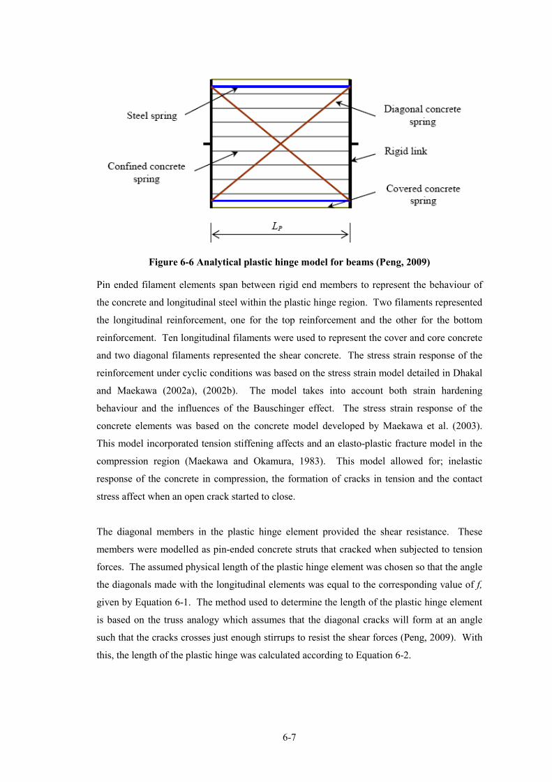
6�7

Figure 6/6 Analytical plastic hinge model for beams (Peng, 2009)

Pin ended filament elements span between rigid end members to represent the behaviour of

the concrete and longitudinal steel within the plastic hinge region. Two filaments represented

the longitudinal reinforcement, one for the top reinforcement and the other for the bottom

reinforcement. Ten longitudinal filaments were used to represent the cover and core concrete

and two diagonal filaments represented the shear concrete. The stress strain response of the

reinforcement under cyclic conditions was based on the stress strain model detailed in Dhakal

and Maekawa (2002a), (2002b). The model takes into account both strain hardening

behaviour and the influences of the Bauschinger effect. The stress strain response of the

concrete elements was based on the concrete model developed by Maekawa et al. (2003).

This model incorporated tension stiffening affects and an elasto�plastic fracture model in the

compression region (Maekawa and Okamura, 1983). This model allowed for; inelastic

response of the concrete in compression, the formation of cracks in tension and the contact

stress affect when an open crack started to close.

The diagonal members in the plastic hinge element provided the shear resistance. These

members were modelled as pin�ended concrete struts that cracked when subjected to tension

forces. The assumed physical length of the plastic hinge element was chosen so that the angle

the diagonals made with the longitudinal elements was equal to the corresponding value of f,

given by Equation 6�1. The method used to determine the length of the plastic hinge element

is based on the truss analogy which assumes that the diagonal cracks will form at an angle

such that the cracks crosses just enough stirrups to resist the shear forces (Peng, 2009). With

this, the length of the plastic hinge was calculated according to Equation 6�2.

6�8

vyv

yc

pfA

sVL =

Equation 6/2

Where Vyc is equal to the shear force which corresponds to the theoretical flexural strength of

the beam, Myc, s relates to the spacing of the stirrups, Av corresponds to the area of the shear

reinforcement and fvy is associated with the yield stress of the shear reinforcement.

The Peng plastic hinge element was found to provide satisfactory predictions of flexural, axial

load and elongation response. However, it did not adequately predict shear deformation due

to yielding of the transverse shear reinforcement. Peng examined the magnitudes of shear

deformation measured in an extended series of beam tests and concluded that, generally, the

total shear deformation in a plastic hinge was of the order of twice the shear deformation from

elongation of the plastic hinge of the beam (from yielding of the longitudinal bars and

cracking of the concrete). Consequently the total shear deformation predicted by the

analytical model was modified to account for the additional shear deformation due to yielding

of the transverse stirrups in the beam.

6.2.4 Mechanisms of Shear Deformation in Walls

There are many similarities and some marked differences in the shear resistance and

deformation response of plastic hinges in structural walls compared to those in beams. The

differences are described in the following paragraphs.

Generally in a beam, the longitudinal reinforcement is concentrated at the top and bottom of

the beam. The shear force is resisted by diagonal compression struts that balance the

longitudinal bond force in the reinforcement and the vertical force from the stirrups. The

diagonal struts extend the full distance between the top and bottom reinforcement as shown in

Figure 6�5. In a wall, the longitudinal reinforcement is spread over the length of the wall and

the bond force is sustained by each bar. Consequently diagonal struts must bear against each

bar with the shear stress rising from the extreme flexural tension bars towards the bars which

are subjected to compression, as illustrated in Figure 6�7.

6�9

Concrete

Zero stress fiber

Longitudinal

reinforcement forces

12

Compression

Tension

(a) Forces in concrete and reinforcing bars

Force in bar 1

Force in bar 2

(b) Shear stresses

Concrete wall

12

Reinforcing bars

(c) Layout of longitudinal reinforcement in wall

Figure 6/7 Shear stresses in wall

The zero stress fibre in the plastic hinge zone of a wall lies closer to the extreme compression

fibre than the extreme tension fibre. A net result of this is that many more longitudinal bars

are subjected to tension forces than bars subjected to compression forces. Therefore under

inelastic loading conditions, the tension forces are considerably greater than compression

forces carried by the reinforcement. This causes the flexural cracks to close in the

compression zone and results in a significant proportion of the total compression force being

resisted by the concrete. The closure of the flexural cracks in the compression zone enables

the compression force to become inclined relative to the longitudinal axis of the wall.

6�10

Shear resisted due to dowel action

Shear transfer by concrete due to inclined compression strut

Tension in longitudinal reinforcement

Tension in transverse reinforcement

Compression in concrete

Figure 6/8 shear transfer of forces in wall

The inclination of this force resists some of the shear, which reduces the shear resisted by the

transverse bars in the wall (as shown in Figure 6�8). Due to this behaviour in a wall plastic

hinge zone, the inclination of the diagonal struts can not be readily determined. This

behaviour does not develop in a beam plastic hinge due to the different geometry.

To overcome the difficulties described above, assumptions were made regarding the plastic

hinge and the inclination of the diagonal struts. The assumptions made for the parameters

used in the wall element are described in Section 6.3.

6.3 Wall Plastic Hinge Element

6.3.1 General

Figure 6�9 illustrates the 2D version of the plastic hinge element. As indicated in the figure

the element has many similarities to the beam element (Peng, 2009).

6�11

Lw

Lp

Lw

Lp

Rigid end memberConcrete

filament

Steel filament

Concrete diagonal spring

Figure 6/9 General layout of analytical wall plastic hinge element

Pin ended filaments which represent the longitudinal reinforcement, core and cover concrete

are spread over the length of the wall. Additional diagonal filaments represent the shear

forces which are resisted by concrete. The stress�strain material models for the concrete and

steel elements were identical to those used in the beam hinge (Peng, 2009) analytical model,

except where mention otherwise in the following sections.

6.3.2 Plastic Hinge Length

The plastic hinge length for this wall element controls the shear stiffness of the wall element

as it controls the angle of the diagonal compression strut. It is therefore not a typical plastic

hinge length which relates to the amount of curvature in the section. The angle of the

diagonal compression strut continuously changes as the wall is loaded and unloaded and the

neutral axis location changes. This behaviour could not be incorporated into the analytical

model at the time of development.

The length of the plastic hinge element was assumed to be equal to the length of the wall,

which results in the diagonal compression strut acting at an angle of 45 degrees. A sensitivity

study was carried out by using different strut angles and comparing the estimates from time

history analysis to experimental results. These comparisons indicated that the results were not

too sensitive to the angle and that an angle of 45 degrees provided a reasonable estimate to the

experimental results.

6�12

6.3.3 Width of Diagonal Strut

The cross sectional area of the diagonal strut was based on the product of the wall thickness

and the effective width dimension which was made equal to 0.55Lw, where Lw is equal to the

length of the wall. Hand analysis which compared the relative stiffness of the diagonal struts

to the horizontal ties (stirrups) showed that the shear deformation was dominated by the

stiffness of the reinforcement and the assumed stiffness of the strut did not have a significant

affect on to the magnitude of shear deformation which developed.

6.3.4 Axial Stiffness of Longitudinal Springs

The flexural stiffness of the beam plastic hinge element is governed by the axial stiffness of

the longitudinal springs. The parameters used to represent the length of the longitudinal steel

springs for beam members were based on the moment distribution principles of a beam

member. These principles are significantly different for a wall member as the internal bars

will most likely not have yielded when the outer bars have first yielded. This method is

therefore not appropriate to determine the length of the steel spring for the wall model. The

length of the steel spring that was used in the analytical model was determined by calibrating

the results from the analytical model to experimental results (Section 6.4). From this

calibration, the length of the steel springs were made to equal the plastic hinge length of the

member. Comparisons between the experimental and analytical results, shown in Section 6.4,

indicated that this length provided reasonable comparisons.

6.3.5 Shear Deformation

As with the Peng method for beams, the wall plastic hinge element could not predict the shear

deformation associated with elastic and inelastic yielding strains in the reinforcement. To

overcome this difficulty, the same assumption that was made in the Peng beam element was

made. That is, the total shear deformation due to strains in the stirrups and the elongation of

the beam hinge region (from yielding of the longitudinal bars and cracking of concrete) was

taken as the product of a coefficient and the deformations associated with the elongation of

the beam hinge region. This coefficient is referred to as the shear flexibility, Vflex, parameter.

The method used to determine the values used for the Vflex parameter is discussed in the

following paragraphs.

To determine the difference between shear deformation from beam elongation and stirrup

extension, reviews of the literature were conducted. It was found that very little experimental

data existed on the components of shear deformations which developed in different types of

walls and only data indicating the total shear deformation of walls during experimental tests

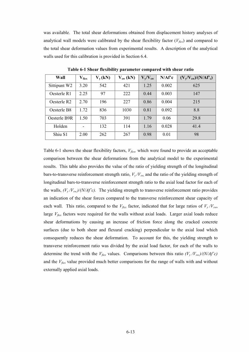
6�13

was available. The total shear deformations obtained from displacement history analyses of

analytical wall models were calibrated by the shear flexibility factor (Vflex) and compared to

the total shear deformation values from experimental results. A description of the analytical

walls used for this calibration is provided in Section 6.4.

Table 6/1 Shear flexibility parameter compared with shear ratio

Wall Vflex Vy (kN) Vsw (kN) Vy/Vsw N/Af’c (Vy/Vsw)/(N/Af’c)

Sittipunt W2 3.20 542 421 1.25 0.002 625

Oesterle R1 2.25 97 222 0.44 0.003 147

Oesterle R2 2.70 196 227 0.86 0.004 215

Oesterle B8 1.72 836 1030 0.81 0.092 8.8

Oesterle B9R 1.50 703 391 1.79 0.06 29.8

Holden � 132 114 1.16 0.028 41.4

Shiu S1 2.00 262 267 0.98 0.01 98

Table 6�1 shows the shear flexibility factors, Vflex, which were found to provide an acceptable

comparison between the shear deformations from the analytical model to the experimental

results. This table also provides the value of the ratio of yielding strength of the longitudinal

bars�to�transverse reinforcement strength ratio, Vy /Vsw, and the ratio of the yielding strength of

longitudinal bars�to�transverse reinforcement strength ratio to the axial load factor for each of

the walls, (Vy /Vsw,)/(N/Af’c). The yielding strength to transverse reinforcement ratio provides

an indication of the shear forces compared to the transverse reinforcement shear capacity of

each wall. This ratio, compared to the Vflex factor, indicated that for large ratios of Vy /Vsw,

large Vflex factors were required for the walls without axial loads. Larger axial loads reduce

shear deformations by causing an increase of friction force along the cracked concrete

surfaces (due to both shear and flexural cracking) perpendicular to the axial load which

consequently reduces the shear deformation. To account for this, the yielding strength to

transverse reinforcement ratio was divided by the axial load factor, for each of the walls to

determine the trend with the Vflex values. Comparisons between this ratio (Vy /Vsw,)/(N/Af’c)

and the Vflex value provided much better comparisons for the range of walls with and without

externally applied axial loads.

6�14

0

0.5

1

1.5

2

2.5

3

3.5

4

0 200 400 600

Sh

ea

r fl

exi

bil

ity

fa

cto

r (V

fle

x)

Transverse capacity - axial load factor

Shear flexibilty factor compared with ratio of

transverse capacity to axial load factor

Analytical Data

Trend

Figure 6/10 Shear flexibility factor compared with ratio of transverse capacity to axial

load factor

The Vflex factor compared to the transverse capacity divided by the axial load factor was

shown in Figure 6�10 to provide, in general, a linear relationship. The relationship for this

linear trend line is represented by Equation 6�3. The parameter x in this equation is related to

the value of the transverse capacity to axial load factor ratio (Vy /Vsw,)/(N/Af’c).

Vflex = 0.0026x+1.748 Equation 6/3

The values obtained from this equation were used in the comparisons between the

experimental and analytical wall results provided in Section 6.4. Variations of the Vflex

parameter in the analytical model indicated insignificant differences between the analytical

and experimental force�shear displacement response.

6.3.6 Contact Stress Parameters

Contact stresses develop between pre�existing flexural and shear cracks as the cracks begin to

close during unloading of reinforced concrete walls. Contact stresses develop before the

cracks are fully closed due to the dislocation of aggregate particles over the cross section of

the wall.

The concrete material model that was used, in the reinforced concrete hinge element, in the

program RUAUMOKO accounts for contact stress by simple linear relationships (shown in

Figure 6�11 where the positive strain denotes tension). These linear relationships are based

on unidirectional push�pull tests as this was the only testing data available on contact stress

behaviour. Magnification parameters, TLIMIT and CLIMIT, were incorporated into the

model to account for the differences which exist in contact stresses between unidirectional

6�15

behaviour, which the loop is based on, and cyclic behaviour. During cyclic behaviour more

cracking will develop in a wall which consequently would result in larger contact stresses

compared to contact stresses in a wall subjected to unidirectional loading. The relationships

of these magnification factors with the contact strain parameters are shown in Figure 6�12.

Figure 6/11 Linear representation of contact stress (Peng, 2009)

(a) Strain at end of contact stress, εcl (b) Strain at start of contact stress, εtl

Figure 6/12 Contact stress parameters and magnification parameters (Peng, 2009)

Where, εtl and εcl are functions of the maximum incremental tension strains, εp is plastic strain,

Fεtmax is the maximum incremental tensile strain and σbo is the residual compression bond

strength which indicates when the contact stress is initiated. CLIMIT and TLIMIT are

parameters controlling the maximum of εtl and εcl. CFACTOR and TFACTOR are used as

multiplication factors on both εtl and εcl to account for the magnification of the contact stress

affect for concrete under tensile and shear actions. The affects of different multiplication

values of CFACTOR and TFACTOR on εtl and εcl is shown in Figure 6�12.

6�16

The residual contact stress parameters used in the experimental wall models were calibrated

against results from the experimental wall tests described in Section 6.4. The residual contact

stress parameters, σbo, that were obtained from the calibration between the experimental and

analytical results are shown in Table 6�2. The axial load factor, N/Af’c, is also shown in this

table for each of the walls as this factor provides an indication of the amount of cracking and

subsequent contact stress which should developed for a wall.

Table 6/2 Contact stress parameter and concrete compressive strength

Wall σbo N/Af’c

Sittipunt � W2 0.15 0.002

Oesterle � R1 0.20 0.003

Oesterle � R2 0.20 0.004

Oesterle � B8 1.00 0.092

Oesterle � B9R 0.80 0.06

Holden � 0.028

Shiu � S1 0.20 0.01

0

0.2

0.4

0.6

0.8

1

1.2

0 0.02 0.04 0.06 0.08 0.1

Co

nta

ct

stre

ss f

acto

r (σ

bo)

Axial load ratio

Relationship between contact stress and

axial load ratio

Analytical Data

Trend

Figure 6/13 Relationship between contact stress and axial load ratio

Figure 6�13 provides a comparison between the contact stress parameter, σbo, and the axial

load ratio for each of the walls for both the calibrated data and a suggested trend line. The

general trend shown in this figure indicates that for walls with lower axial load ratios, a lower

contact stress parameter results. Greater dislocation of the concrete is expected to occur for a

wall with a lower axial load ratio, due to the development of more cracking from lower

strength concrete and gaps not closing as well for a wall with a low applied axial load. The

6�17

dashed line shown in this figure indicates the trend line; the equation for this line is given by

Equation 6�4. The parameter x in this equation refers to the axial load ratio.

Contact stress = 9.70x+ 0.148 Equation 6/4

The contact stress parameter suggested by Peng (2009) for beam members was 0.2. This

value was found to be adequate for walls which resisted gravity loads only. The factors

which affect the magnitude of the strain which represents the start and the finish of the contact

behaviour were found to provide reasonable results for all walls with values of 1.5 for the

start and 1.0 for the finish are acceptable. These values are similar to the values

recommended by Peng (2009) for beam members.

The analytical model used in the comparisons between the experimental and analytical wall

results, shown in Section 6.4, included the parameters from Equation 6�4. The comparisons

with the experimental wall results indicate small variations of the contact stress parameter do

not significantly affect the response from the analytical model.

6.3.7 Modifications made to the Beam Plastic Hinge Model

Modifications were made to the beam plastic hinge analytical model (Peng, 2009). Simple

studies revealed that the Peng model, available in the current version of RUAUMOKO, was

not predicting adequate results compared to analytically calibrated experimental results. A

number of modifications were made to the current version of RUAUMOKO to fix the beam

hinge model. A summary of the modifications are listed in the following bullet points, details

to these are provided in the following paragraphs:

− The reinforced concrete material model;

− The stiffness representation of the filament springs;

− Inclusion of bi�linear factors;

− Sign changes within the FORTRAN code;

− Changes to the format of the FORTRAN code relating to the adjustment for shear

flexibility due to stirrup elongation.

The reinforced concrete material model that was used to represent the concrete material

behaviour, in the plastic hinge model, was found to have some analytical continuity problems

between the loading and unloading paths. When the material strains reached a discontinuity

in the model the path was lost and the model resulted in incorrect response. All possible

unloading, reloading, compression, tension and contact stress paths for each of the regions in

the material model were checked, and modified if required, to ensure that continuity existed

6�18

between all paths in the model. Checking of the continuity was done by reviewing the

FORTRAN code that described the material behaviour and checking the material hysteresis

plots, for different loading cases, by the use of the program HYSTERES (Carr, 2004�2010).

In the original hinge model the initial stiffness was used to represent the stiffness of the

filament springs for the entire analysis. The beam hinge model was modified to use the

tangent stiffness during the analysis rather than using the constant initial stiffness. This

required the derivatives of the stress, with respect to strain, to be determined for each of the

loading�unloading compression�tension paths in the material model.

A bi�linear factor was added to the plastic hinge element to allow the strain hardening of steel

to be represented by the analytical model. In the available model, from RUAUMOKO, no bi�

linear factor was supplied. In addition, a number of corrections were made to the FORTRAN

code where incorrect signs were used in the analytical model.

In the beam hinge model, shear flexibility due to stirrup elongation could not be directly

modelled. To allow for this, a shear flexibility factor, which increased the total shear

deformation of the element, was incorporated. In the original beam hinge model, the total

shear was adjusted to account for the shear flexibility, but was not adjusted back to ensure

equilibrium was maintained in the analytical model. The analytical model was left to find

equilibrium by itself, which was found to cause some numerical stability problems in the

results. The shear deformation in the analytical model was consequently adjusted back to

equilibrium within the program to avoid the problems which developed.

After the changes to the beam hinge element had been made comparisons of the estimates

from time history analysis were made to experimental results. Reasonable comparisons were

obtained.

6.4 Experimental Comparisons

Experimental data for eight different walls was obtained from the literature. Each of these

walls had different properties such as: aspect ratios, reinforcement ratios, concrete strengths,

steel strengths and applied axial loads. The walls included in the comparison were chosen to

ensure a range of walls with different geometric and material properties were included in the

comparisons.

6�19

6.4.1 General

The analytical modelling parameters used for each of these analytical wall models were

obtained from the suggested values given in Section 6.3.

General comparisons between the experimental and analytical results indicted there are some

discrepancies in the initial measured and predicted deformations in the elastic cycles. This is

likely to be due to assumptions made regarding the initial elastic properties of the concrete,

deformation of the response in the base pad of the wall and the variations in the initial stresses

in the concrete associated with shrinkage of the concrete. In view of the overall deformation

sustained by the wall, the relatively small discrepancies of deformation in the pre�yielding

range are of little significance.

Some of the wall hysteresis plots, showing the results for the analytical wall model, were

observed to develop sudden spikes (sometimes referred to as ringing effects) at locations

where displacement reversals occurred. These spikes developed due to sudden changes of

stiffness of the wall causing local convergence problems. These spikes were found to be most

prominent in the analytical model representing the Oesterle�R2 wall. This wall has a very

high proportion of boundary reinforcement and compressive concrete strength which, when

the loading direction changed, a large change in stiffness of the different materials which

were taking the load occurred. The Shiu�S1 wall also had a large boundary reinforcement

ratio. Ringing effects were not present for this wall due to the low concrete compressive

strength.

6.4.2 Sittipunt – W2

Experimental wall tests were carried out by Sittipunt et al. (2001) to determine the influence

of diagonal web reinforcing steel on the hysteretic response of the wall. For this study four

walls were constructed, two walls with conventional horizontal and vertical reinforcement and

two with inclined diagonal web reinforcement. Wall, W2, from these experimental tests had

conventional horizontal and vertical reinforcement; this wall was used in the comparisons for

this study. The walls were designed using the procedures in the ACI Building Code (ACI318�

99) for regions of low and moderate seismic risk. The assumed concrete design strength was

29MPa and the yield stress of the reinforcing steel was 390MPa. A single layer of web

reinforcement (horizontal) was used in the walls, consistent with design practice in Thailand

in 2001, which was equivalent to 1/5 of the transverse reinforcement required in the United

States (ACI Committee 318, 2008). The geometry and reinforcing details of this wall are

shown in Figure 6�14.

6�20

1900mm

1000mm

1500mm

500mm

Horizontal loading

7 10mmΦ

250mm

25

0m

m

100mm

6 16mm and

2 2mm

ΦΦ1

Φ10 at 100mm

Φ6 at 100mm

Figure 6/14 Geometry and reinforcing details for Sittipunt et al. (2001) wall W2

The geometry of this was wall was barbell shape with a thin web and a height to length aspect

ratio of 1.43. The longitudinal reinforcement ratios for this wall were 2.3% in the boundary

elements and 0.5% in the web and the transverse reinforcement ratio was 0.8%. The

measured compressive strength of the concrete was 36MPa and the size and yield strengths of

the reinforcing bars were: 10mm: fy=450MPa, 16mm: fy=473MPa and 12mm: fy=425MPa.

Only one tensile strength can be assigned to represent the strength of the reinforcing bars in

the analytical model. Therefore, an average area weighted value (of the flexural boundary

element reinforcement) of 461MPa was used in the analytical model.

The wall was subjected to cyclic displacement controlled loading. The peak displacements

were increased from a displacement ductility of 1 to a displacement ductility of 5 with three

cycles per ductility level. The results indicated that large shear deformations developed

during the displacement ductility 5 cycle. The analytical wall model has not been developed

to represent failure behaviour in shear. Therefore, comparisons were made between the

analytical and the experimental results up to the displacement cycle of ductility 4.

6�21

Figure 6/15 Shear force versus top of wall displacement for Sittipunt W2

Figure 6�15 shows the comparison between the experimental results and the analytical results

for the Sittipunt wall, W2. This comparison indicates that the analytical model adequately

represented the results, particularly for the positive quadrant response. The analytical

predictions do not match the results in the negative quadrant as well. This is possibly due to

the shear distortions that developed due to significant crushing of the web. The web crushing

was not captured in the analytical model as the shear behaviour is represented by two

diagonal springs which represents the average shear behaviour and not the behaviour of each

individual diagonal compression strut, which would form in reality.

6�22

Figure 6/16 Shear force versus total shear distortion for Sittipunt W2

Comparisons between this analytical wall model and the experimental results, shown in

Figure 6�16, indicate that the analytical model adequately predicts the shear distortion

behaviour up to the point where the shear failure begins to occur at +/�0.15 radians.

6.4.3 Oesterle – R1

Experimental tests were carried out by Oesterle et al. (1976) to improve understanding

associated with the strength and deformation behaviour of walls. Nine wall specimens were

tested in this experimental study. Each specimen was loaded as a vertical cantilever with

forces applied through a slab attached to the top of the wall. Analytical models, using the

proposed wall element, were developed to represent wall R1, R2, B8 and B9R from this

experimental study.

The design moments for the walls were calculated following the 1971 ACI Building Code.

The design concrete strength was taken as 41.4MPa and the strength of the flexural

reinforcement was 414MPa. A range of different methods were used to design the shear

reinforcement for the walls. For wall R1, R2 and B9R the horizontal shear reinforcement was

determined using the minimum requirements of the 1971 ACI Building Code as this governed

6�23

the design. For wall B8, the shear reinforcement was determined using the shear force

corresponding to the calculated maximum moment capacity of the wall, which incorporated

strain hardening affects of the longitudinal bars. The results from wall R1 are discussed in

this section and the results for the other walls are discussed in Sections 6.4.4 to 6.4.6.

4369mm

203mmHorizontal

loading

102mm

1905mm

Centreline4D9.5mm 6mm

6mm

Figure 6/17 Wall geometry and reinforcing details for Oesterle R1

The geometry and reinforcing details for wall R1, from the experimental study, are shown in

Figure 6�17. This wall was rectangular in geometry with an aspect ratio of 2.35 and a width

of 0.102m. The boundary and web longitudinal reinforcing ratios for this wall were 1.47%

and 0.25% respectively. The transverse reinforcement ratio was 0.31%. The measured

compressive strength of the concrete was 45MPa and the tensile strength of the reinforcing for

the 9.3mm bars and 6mm bars were 512MPa and 522MPa respectively. The capacity used in

the analytical model was 512MPa which was the strength of the flexural reinforcement. This

wall had no external axial loads applied to it.

The displacement loading that was applied to this specimen was applied in cycles of three.

The maximum displacement that was applied to this specimen was 0.127m. The experimental

results indicated that during the maximum displacement cycle reinforcing bars began to

fracture. As this model can not predict the failure behaviour, for this comparison with the

analytical wall results the maximum displacement cycle that was applied was 0.102m.

6�24

Figure 6/18 Shear force versus top of wall displacement for Oesterle R1

Figure 6�18 indicates that generally a reasonable fit between the experimental and analytical

results was obtained except at small displacements the analytical model over predicts the

forces. The analytical model predicts the forces, displacements and contact forces adequately

up until the point where the first bar was observed to fracture in the experimental test at

displacements of +/�0.1m.

6�25

Figure 6/19 Shear force versus total shear distortion for Oesterle R1

Comparisons between the analytical wall model and the experimental shear results for this

wall indicate that the analytical model adequately predicts the general shear force – shear

distortion behaviour. However initial loading and displacements under reversed direction of

loading were not modelled satisfactorily.

6.4.4 Oesterle – R2

This wall was part of the experimental testing regime that was carried out by Oesterle et al.

(1976) for the wall described in Section 6.4.3. The geometry and reinforcing details for this

wall are provided in Figure 6�20.

6�26

4369mm

203mmHorizontal

loading

102mm

1905mm

Centreline6D12.7mm 6mm

6mm

Figure 6/20 Wall geometry and reinforcing details for Oesterle R2

The geometry of this wall was rectangular shape with a height to length aspect ratio of 2.35

and width of 0.102m. The boundary and web longitudinal reinforcing ratios for this wall

were 4.0% and 0.25% respectively and the transverse reinforcement ratio was 0.31%. The

geometry and reinforcement details for this wall were similar to the Oesterle R1 with the

exception of much larger boundary reinforcement. The measured compressive strength of the

concrete was 46MPa and the yield strength of the reinforcing for the 12.7mm bars and 6mm

bars were 450MPa and 535MPa respectively. The capacity used in the analytical model was

450MPa which was the strength of the predominant flexural reinforcement. This wall had no

external axial loads applied to it.

The displacements that were applied to this wall were similar to the displacements applied to

Oesterle R1. The maximum displacements applied to this wall were 0.152m, with 0.127m

used for this comparison with the analysis of wall Oesterle R1, as reinforcing bars were

observed to fracture in the experimental test during displacements of 0.152m.

6�27

Figure 6/21 Shear force versus top of wall displacement for Oesterle R2 wall

Figure 6�21 indicates that the analytical wall model used to represent the behaviour of the

Oesterle R2 wall provides a reasonable prediction of the results, except for the over�prediction

of force during initial loading. The wavy response along the yield plateau is due to the

ringing affects in the analytical model due to sudden changes of stiffness in the analytical

model, this is discussed in Section 6.4.1. The response is wavy rather than sharp as the data

points for this figure were plotted for every 200 steps rather than every step to reduce the size

of the data file. The analysis of the wall model was stopped before the bars were observed to

fracture in the experimental test.

6�28

Figure 6/22 Shear force versus total shear distortion for Oesterle R2

Comparisons between the analytical wall and the experimental shear results, showing in

Figure 6�22, for this wall indicate that the analytical model adequately predicts the general

shear force � shear distortion behaviour after first yield of the longitudinal bars in the wall.

The analytical model was again unable to predict large shear deformations as the model failed

to predict the contact stress behaviour as accurately.

6.4.5 Oesterle – B8

The experimental wall testing that was carried out by Oesterle et al. (1976) was extended by

Oesterle et al. (1979) to further investigate the behaviour of walls. Wall B8 from this

experimental study was used to help to verify the analytical model. The geometry and

material properties for this wall are provided in Figure 6�23

6�29

4369mm

1295mm

2362mm

203mmHorizontal

loading

305mm

305

mm

102mm

1295mm

1905mm

12D19mm6mm 6mm

Figure 6/23 Wall geometry and reinforcing details for Oesterle B8

The geometry of this wall was a barbell shape with a height to length aspect ratio of 2.35, a

web width of 0.102m and flange width of 0.305m. The boundary and web longitudinal

reinforcing ratios for this wall were 3.7% and 0.3% respectively. This wall had a transverse

reinforcement ratio of 1.38% which is greater than the transverse reinforcement ratios for the

other experimental walls that were used in this comparison. The compressive strength of the

concrete was 42MPa and the tensile strength of the reinforcing bars for the #6 bars and 6mm

bars were 447MPa and 454MPa respectively. This wall had an external axial load of 1164kN

applied to it.

The maximum displacement applied to this wall was 0.152m, for this displacement web

crushing was observed to occur. Again, for the comparison between the analytical and

experimental results a maximum displacement of 0.127m was used.

6�30

Figure 6/24 Shear force versus top of wall displacement for Oesterle B8 wall

Figure 6�24 indicates the analytical model predicts the behaviour of the experimental wall

reasonably well.

Figure 6/25 Shear force versus total shear distortion for Oesterle B8

6�31

Figure 6�25 indicates the comparisons between the analytical wall and the experimental shear

results for this wall, these results indicate similar trends to the trends shown for Oesterle R1.

These comparisons indicted that the analytical model adequately predicted the general shear

force�shear distortion behaviour but did not predict the unloading behaviour as well.

6.4.6 Oesterle – B9R

The Oesterle B9R wall was part of the experimental testing program that was carried out by

Oesterle et al. (1979), similar to wall B8. Wall B9R was a repaired version specimen Wall

B9. The web of specimen B9 was damaged after testing, but the columns and reinforcement

in the columns were in good condition. The maximum measured crack widths in the columns

of 1.4mm on the tension side and 0.2mm on the compression side from the peak load. The

concrete in the web of this wall was replaced to 3.7m of height of the wall, from the base; the

reinforcing bars were not changed. Wall B9R was modelled by the analytical wall element to

help to verify the analytical model. The geometry and material properties for this wall are

provided in Figure 6�26.

4369mm

1295mm

2362mm

203mmHorizontal

loading

305mm

30

5m

m

152mm

1295mm

1905mm

12D19mm6mm 6mm

Figure 6/26 Wall geometry and reinforcing details for Oesterle B9R

The geometry of this wall was a barbell shape with a height to length aspect ratio of 2.35, a

web width of 0.152m, which was thicker than the other walls, and flange width of 0.305m.

The boundary and web longitudinal reinforcing ratios for this wall were 3.7% and 0.2%

respectively and a transverse reinforcement ratio of 0.42%. The compressive strength of the

concrete was 52MPa and the tensile strength of the reinforcing for the #6 bars and 6mm bars

were 430MPa and 461MPa respectively. Strain hardening of the reinforcing bars was not

accounted for in these strength values. This wall had an additional axial load of 1190kN

applied to it.

6�32

The maximum displacement applied to this wall was 0.241m, for this displacement web

crushing and bar fracture was observed to occur in the experimental testing. For the

comparison between the analytical and experimental results a maximum displacement of

0.178m was used.

Figure 6/27 Shear force versus top of wall displacement for Oesterle B8 wall

Figure 6�27 indicates the analytical model predicts the loading behaviour of the wall

reasonably well. This analytical model of the wall is shown to not predict the unloading

stiffness as well for large displacement cycles compared to smaller displacement cycles.

6�33

Figure 6/28 Shear force versus total shear distortion for Oesterle B9R

Comparisons between the analytical wall and the experimental shear results, shown in

Figure 6�28 for this wall indicate that the analytical model did not predict the initial behaviour

well. This is most likely due to this wall having been previously tested and then repaired.

The analytical model seems to adequately predict the shear deformation and the yielding

shear force for the inelastic displacement cycles. The unloading behaviour is also predicted

reasonably well.

6.4.7 Holden Wall

Two experimental wall tests were carried out by Holden et al. (2001) to investigate the change

in performance between a conventionally reinforced wall and a hybrid wall which

incorporated post�tensioned un�bonded carbon fibre tendons and steel fibre reinforced

concrete. The conventionally reinforced wall was used in this study. The conventional wall

was design for ductile response using the procedures presented in the Concrete Structures

Standard (NZS3101:1995). It was found during the design a number of minimum

requirements governed. Figure 6�29 indicates the geometry and reinforcing details for this

wall.

6�34

3.75m

125mm

1.35m

CL6HD10

Cover 6mm

R6

675mm

F

Hd10

Figure 6/29 Wall geometry and reinforcing details for Holden wall

The shape of this wall was rectangular with a height to length aspect ratio of 3.75m and width

of 0.125m. The boundary and web longitudinal reinforcing ratios for this wall were 1.25%

and 0.6% respectively. The transverse reinforcement ratio for this wall was 0.25% which is

the smallest for all of the walls included in this verification study. The compressive strength

of the concrete was 46MPa and the tensile strength of the longitudinal reinforcing bars was

476MPa. This wall had an additional axial load of 200kN applied to it. The testing schedule

used for this wall was displacement controlled with a maximum drift angle of 3%.

Figure 6/30 Shear force versus top of wall displacement for Holden wall

6�35

Figure 6�30 indicates that the results from the analytical model over�predict the experimental

data. Reviews of the observations of the response of the wall during the experimental tests

provided no insight as to why the strength was over predicted by this analytical model. The

strength is shown in this figure to be over predicted from the beginning of the analysis. This

suggests that a material strength property could possibly have been incorrectly recorded in the

report that detailed the experimental test.

6.4.8 Shiu – S1

Two 1/3�scale structural walls were experimentally tested by Shiu et al. (1981) to investigate

the affects of openings in walls. One of the walls in this experimental test had openings and

the other did not. For this study the wall with no opening was used for comparisons with the

analytical model. These walls were design as coupled wall systems by following the

provisions in the 1971 ACI Building Code and the 1976 Uniform Building Code. The

concrete and steel material strengths that were used in the design were respectively 20.7MPa

and Grade 60 steel (minimum yield strength of 414MPa). The geometry and material

properties of this wall are shown in Figure 6�31.

5.486m

Horizontal loading

102mm

1.905m

12D12.7mm 6mm

6mm

0.71m

0.610m

0.064m

0.102m

953mm

Centreline

Figure 6/31 Wall geometry and reinforcing details for Shiu, S1

This wall was rectangular in geometry with diaphragm stubs at certain levels of the wall. The

wall had a height to length aspect ratio of 2.88 and a width of 0.102m. The diaphragm stubs

were not used to provide vertical loads or act as points for horizontal loading and therefore

would not greatly affect the overall performance of the wall. The boundary and web

longitudinal reinforcing ratios for this wall were 4.8% and 0.26% respectively and the

6�36

transverse reinforcement ratio for this wall was 0.42%. The measured compressive strength

of the concrete was 23MPa and the tensile strength of the reinforcing bars for the 12.7mm

bars and 6mm bars were 476MPa and 473MPa respectively. This concrete compressive

strength was the lowest for all of the walls included in this comparison study. This strength

was less than the recommended range of concrete compressive strengths provided in the New

Zealand Concrete Structures Standard (Standards New Zealand, 2006). This wall did not have

any external axial load applied to it.

Figure 6/32 Shear force versus top of wall displacement for Shiu S1 wall

This comparison indicates that the analytical model provides a reasonable prediction of the

experimental results including the unloading affects.

6�37

Figure 6/33 Shear force versus total shear distortion for Shiu S1

Comparisons between the analytical wall and the experimental shear results shown in

Figure 6�33, for this wall, indicate that the analytical model adequately predicts magnitudes of

the shear force and total shear distortion. The analytical model does not predict the reloading

stiffness well though. The experimental results for this specimen indicated that several

horizontal cracks developed along the bottom level of the wall, with a major horizontal crack

forming at 0.46m from the base of the wall. These cracks lead to sliding behaviour of the

wall. This analytical model is unable to represent sliding behaviour and dowel action of the

longitudinal bars. The inability to predict sliding behaviour for this wall resulted in less shear

distortion at the end of the contact phase resulting in a poor (more flexible) prediction during

the reloading phase.

6.5 Limitations of Model

The results from this study have indicated that parameters used to represent the wall

behaviour vary depending on parameters such as the: concrete strength, axial load and

yielding (of longitudinal bars) strength to transverse reinforcement ratio. A range of walls

with a variety of these parameters were included in this study. This model should not be used

for walls outside of the ranges of the parameters of the walls included in this experimental

comparison. The range of allowable parameters is provided in the following:

6�38

− The yielding strength (of longitudinal bars) to transverse reinforcement ratios and

axial load factors were used to determine the shear flexibility factors (Section 6.3.4)

and contact stress parameters (Section 6.3.6) in the analytical model. The limits for

the yield strength to transverse reinforcement ratio were between 0.44 and 1.79 and

the limits for the axial load factors were 0.002 to 0.092;

− This model is not to be used to represent the behaviour of walls with large axial loads

such as coupled walls. Only a limited number of comparisons were made between

the analytical results and experimental results for walls with external loads that were

greater than gravity loads;

− This analytical model should only be used for walls with longitudinal and transverse

reinforcement layouts. The steel filament springs which represent the reinforcement

in this model represent these layouts;

− The analytical model was found for some of the comparisons in Section 6.4 to

provided poor representations of the experimental results for small displacements.

This model should only be used for walls which are exposed to displacements which

are greater than the expected yield displacement of the wall where consideration is

given to the cracked stiffness values;

− The analytical wall model was found to poorly predict the unloading stiffness for a

small number of the comparisons indicated in Section 6.4. Poor predictions of the

unloading stiffness could affect the response of other members when exposed to small

forces. This analytical model should therefore only be used where the maximum

responses are of interest.

This analytical wall model was developed to represent the walls used in the torsion study

carried out in Chapter 7. The axial loads that were expected to develop in these walls were

predominantly gravity loads. A calculation to determine the axial loads indicate that axial

load ratio of around 0.015 would be expected. An axial load of this magnitude can be

adequately represented by this analytical model.

6.6 References

ACI Committee 318 (2008). Building Code Requirements for Structural Concrete (ACI318�

08) and Commentary. American Concrete Insitute.

Carr, A. J. (2004�2010). Computer Program Library: Hysteres. Christchurch, New Zealand,


6�39

Dhakal, R. P. and Maekawa, K. (2002a). "Modeling for Postyield Buckling of

Reinforcement." Journal of Structural Engineering 128(9): 1139�1147.

Dhakal, R. P. and Maekawa, K. (2002b). "Reinforcement Stability and Fracture of Cover

Concrete in Reinforced Concrete Members." Journal of Structural Engineering

128(10): 1253�1262.

Fenwick, R. C. and Davidson, B. J. (1995). "Elongation in Ductile Seismic�Resistant

Reinforced Concrete Frames." ACI SP�157 Recent Developments in Lateral Force

Transfer in Buildings: 143�170.

Fenwick, R. C. and Fong, A. (1979). The Behaviour of Reinforced Concrete Beams under

Cyclic Loading. Report No 176, University of Auckland, Auckland, New Zealand.

Fenwick, R. C. and Megget, L. M. (1993). "Elongation and Load Deflection Characteristics of

Reinforced Concrete Members Containing Plastic Hinges." Bulletin of the New

Zealand National Society for Earthquake Engineering 26(1): 28�41.

Fenwick, R. C. and Thom, C. W. (1982). Shear Deformation in Reinforced Concrete Beams

Subjected to Inelastic Cyclic Loading. School of Engineering Research Report

Auckland, University of Auckland. 279.

Holden, T., et al. (2001). A comparison of the Seismic Performance of Precast Wall

Construction: Emulation and Hybrid Approaches. Christchurch, Department of Civil

Engineereing, Univeristy of Canterbury. 2001�04.

Lee, J. Y. and Watanabe, F. (2003). "Predicting the Longitudinal Axail Strain in the Plastic

Hinge Regions of Reinforced Concrete Beams Subjected to Reversed Cyclic

Loading." Engineering structures 25(7): 927�939.

Maekawa, K. and Okamura, H. (1983). "The Deformation Behaviour and Constitiutive

Equation of Concrete Using Elastic�Plastic and Fracture Model." Journal of Faculty

of Engineering, University of Tokyo 37(2): 253�328.

Maekawa, K., et al. (2003). Nonlinear Mechanics of Reinforced Concrete. London, Spon

Press.

Oesterle, R. G., et al. (1979). Earthquake�Resistant Structural Walls � Tests of Isolated Walls:

Phase 2. Report to National Science Foundation. Skokie, Illinois, Construction

Technology Laboratories, Portland Cement Association: 338.

6�40

Oesterle, R. G., et al. (1976). Earthquake�Resistant Structural Walls � Tests of Isolated Walls,.

Report to National Science Foundation,. Skokie, Illinois, Construction Technology

Laboratories, Portland Cement Association,: 315.




Shiu, K. N., et al. (1981). Earthquake Resistant Structural Walls � Tests of Walls With and

Without Openings, Construction Technology Laboratories, Portland Cement

Association, Skoki, Illinois.

Sittipunt, C., et al. (2001). "Cyclic Behaviour of Rieinforced Concrete Structural Walls with

Diagonal Web Reinforcement." ACI Structural Journal 98(4): 554�562.



7�1

7 TORSION STUDY

7.1 Introduction

A newly proposed force based floor diaphragm design method, the pESA method, is

described in Chapter 5. The intention of the torsion study described in this Chapter was to

verify the pseudo�Equivalent Static Analysis (pESA) method for the use with torsionally

susceptible dual structures (about the vertical axis). This torsion study was carried out to

determine how torsion affects the response of the structure and what limitations should be

placed on the use of the pESA method with regard to torsionally susceptible dual structures.

A range of analytical models with dual structural systems were developed and analysed using

non�linear numerical integration analyses. These structures had a range of strength, stiffness

and mass eccentricities. The structural systems investigated were torsionally restrained

structural systems. Torsionally restrained refers to a structural system which has lateral force

resisting elements in at least two planes (Paulay, 2001).


Design of torsionally susceptible structures was traditionally based on eccentricity of the

centre of mass of each floor from the centre of (lateral) stiffness of the lateral force resisting

elements (walls and frames). This perspective was based on the elastic behaviour of the

system. However, the torsion about the vertical axis of a building that results from

eccentricity of the centre of mass for the centre of strength (elastic and inelastic ranges) was

typically ignored. Recent research (Priestley and Kowalsky (1998), Paulay (2000)) has

highlighted that stiffness is dependent on strength, which is contrary to the traditional

assumption that strength and stiffness were independent. This finding of the inter�dependence

of stiffness and strength has made the assumptions used in traditional torsional design

methods incorrect. As a result of this, researchers (Castillo (2004), Paulay (1999), Beyer

(Beyer, 2007) and Priestley et al. (2007)) have developed displacement based “desktop”

methodologies for designing asymmetric structures that incorporate the inter�dependence of

strength and stiffness.

7.2.1 Paulay (2001)

Paulay (2001) suggested that strength eccentricities in a system could be equally, if not more,

significant than stiffness eccentricities. It was discussed that during elastic dynamic response

7�2

of a structure, the stiffness eccentricities would control the torsional response and when the

system began to deform inelastically, the strength eccentricities would dominate. It was

suggested that the design of torsionally susceptible structures should follow a strength

approach as the designer has full control over the distribution of strength of the structure.

Paulay’s paper discussed some design aims for the design of torsional structures. The focus

of these aims was related to earthquake�induced displacements in buildings with adequate

strength. These aims included:

− Displacements observed to develop, due to seismic attack, should be less than the

ductility capacity of the elements of the structure;

− Inter�storey drifts of elements away from the centre of mass should be less than the

maximum acceptable inter�storey drift limits;

− Checks should be carried out to ensure that the displacements of individual structure

elements satisfy the design criteria including not excluding the plastic rotation

capacities of the elements.

7.2.2 Castillo (2004)

An analytical study was carried out at the University of Canterbury by Castillo (2004) on

asymmetric ductile structures. The focus of Castillo’s study was to develop a better

understanding of the response of torsionally susceptible structures and to subsequently

develop a simple design strategy for these structures. The analytical results were found to be

in satisfactory agreement with the results from laboratory tests.

Castillo carried out a multi�dimensional parametric study to identify the parameters which

influenced the torsional behaviour of structures. The parameters included: strength

eccentricity, mass eccentricity, the ratio of the radii of gyration of both strength and mass of

the system, changes in the system displacement ductility capacity, the influence of transverse

elements on torsional restraint of the system, different ratios of nominal yield displacement

for different elements in the system, stiffness eccentricity of the elements and uncoupled

translational periods. The analyses were made using a range of different earthquake records

and different application orientations.

The in�plane behaviour of one storey building was modelled. Multi�storey affects were not

considered. The material behaviour of the wall elements were modelled with an elasto�plastic

hysteretic model. The following conclusions were made:

7�3

For torsionally restrained structures which have lateral force resisting elements in at least two

planes (Paulay, 2001):

− Rotations were restricted by mass rotational inertia and further reduced by transverse

elements which were perpendicular to the direction of the earthquake forces;

− Variations in the distribution of strength and mass were found to have a small affect

on displacement demands;

For torsionally unrestrained structures which have lateral force resisting elements in one

plane only:

− The mass rotational inertia reduces the system rotations expected to occur compared

to results were mass rotation inertia is not incorporated in the model;

− Stiffness and strength eccentricities were found to have a large affect on the

displacement demands;

− Strength eccentricity was the predominant parameter that influenced the response of

the ductile system;

− Rotations about the vertical axis that develop in the system, due to torsion, could be

managed by ensuring that adequate displacement capacity of the structural elements

was provided.

The results from Castillo’s study lead to the development of a proposed design strategy. An

overview of this is provided in the following steps:

1. The displacement ductility capacity of the system is determined by obtaining the

displacement ductility capacity of the elements in the system using displacement

based design method (Priestley et al., 2007). This type of design is based on a single

degree of freedom structure representation which indicates the performance at peak

displacement response.

2. The nominal strengths are then assigned to the system with the aim of minimising

strength eccentricity:

a. A check should be made to ensure that the assigned nominal strength does

not exceed the previously established capacity of the elements.

3. It was recognised that due to variable tolerances in detailing, construction and

codified requirements of maximum and minimum reinforcement ratios, removing

strength eccentricity in a system, in some cases, can not easily be achieved.

Therefore strength eccentricity can be tolerated on the condition that the nominal

strength of the lateral force resiting elements is greater than the strength required to

obtain zero strength eccentricity in the system.

7�4

4. Accidental eccentricities are recommended to be dealt with as per current code

recommendations.

The justification of this methodology was that the total displacement demand on the critical

element of the system (exposed to both translational and rotational displacements) should not

exceed the displacement capacity of the element. This is illustrated in Figure 7�1 and the

symbols shown in this figure are defined in Table 7�1.

Figure 7'1 Rational of the proposed design strategy (Castillo, 2004)

Table 7'1 Description of symbols shown in Figure 7'1

�d Design displacement of system

�ue1 Displacement demand or capacity of element 1

�ue2 Displacement demand or capacity of element 2

�us Displacement demand or capacity of system

�ye1 Displacement at first yield for element 1

�ye2 Displacement at first yield for element 2

�ys Nominal yield displacement of system

ev Strength eccentricity of system

er Stiffness eccentricity of system

θ System rotation

Vns Excess nominal strength of system

Vnsx Nominal strength assigned to system

7.2.3 Priestley (2007)

The book by Priestley (2007) provides reference on how to deal with torsionally sensitive

structures in the framework of displacement based design. This book presents methodologies

7�5

to deal with the design of the lateral force resisting system for both torsionally restrained and

unrestrained structures. Predictions from the proposed method of analysis were compared

with time history analysis of structures reported by Castillo (2004) and Beyer (2007). The

proposed method was found to provide reasonable comparisons to the displacements at the

extremities of the structure from the displacements obtained from time history analyses. This

method is described in the following paragraphs.

The maximum displacement of the building is obtained by determining the translational

displacement of the building by using Direct Displacement Base Design (DDBD) principles

and determining the rotation of the building from Equation 7�1.

θN = VBase . eR / JR,� Equation 7'1

Where VBase is the design base shear, eR is the elastic stiffness eccentricity and JR,� is the

modified elastic rotational stiffness (details with how to calculate these values can be found in

the book).

From this, the displacements at the end walls are then obtained from Equation 7�2, where �CM

is the displacement at the centre of mass, xi is the distance from the centre of mass and ev is

the strength eccentricity.

�i = �CM + θN . (xi – ev) Equation 7'2

For displacement based design, Equation 7�2 is reorganised to determine the displacement at

the centre of mass with �i representing the limit drift of the lateral force resisting element (for

both torsional and translational displacement) from the code. To obtain the design

displacement an iterative process, with respect to determining the torsional displacements,

may be required.

It was recommended in this text that the best design solution for torsionally susceptible

structures was to eliminate, as best possible, any strength eccentricity in the system. If this is

not possible the strength eccentricities of the system should be minimised.

No details were provided in this book regarding how to deal with the design of floor

diaphragm for torsionally susceptible structures.

7�6

7.2.4 New Zealand Loadings Standard: NZS1170.5

The New Zealand Design Actions Standard, NZS1170.5 (Standards New Zealand, 2004a)

provides some limitations for the use of static methods in relation to the torsional

susceptibility of structures. It is stated that 3D modal analysis or a special study, such as

numerical integration time history analysis, shall be used for structures that are classified as

torsionally sensitive. A structure is classified as torisonally sensitive by the New Zealand

Design Actions Standard when γ, defined in Equation 7�3, exceeds 1.4.

γ = Max( γi = dmax/dav) Equation 7'3

Where γ is the maximum value for each orthogonal direction, γi is the ratio for each level i, dav

is the average of the displacements at the extreme points of the structure at level i and dmax is

the maximum of the storey displacements at the extreme points of the structure induced by the

equivalent static actions (centred at +/� 0.10 times the plan dimension of the floor,

perpendicular to the load direction).

7.3 What is the Purpose of this Study?

This review of the literature indicated that to this point there is no research regarding floor

diaphragm design methods for torsionally sensitive structures. The aim of this study was to

determine how torsionally susceptible dual structures affect the magnitudes of floor

diaphragm forces. In addition to this, it was envisaged that the results from this study would

give an indication of the limits of the use of the proposed pESA floor diaphragm method with

regard to torsionally sensitive structures.

Reviews of the literature indicated distinct differences between torsionally restrained and

torsionally unrestrained structures. It was found in the studies carried out by Castillo that the

influence of strength and mass eccentricites were less for torsionally restrained structures

compared to unrestrianed structures. From these findings, it was decided for this torsion

study, only torsionally restrained structures would be considered. Consideration of the ability

of the pESA method to predict the behaviour of torsionally unrestrained structures could be a

possible avenue of future research.

7.4 Description of Analyses

7.4.1 General

Four dual buildings, which contained moment resisting frames and structural walls, were

analysed to study the affects of torsion. A general plan view of these buildings is shown in

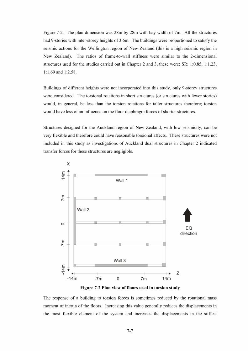
7�7

Figure 7�2. The plan dimension was 28m by 28m with bay width of 7m. All the structures

had 9�stories with inter�storey heights of 3.6m. The buildings were proportioned to satisfy the

seismic actions for the Wellington region of New Zealand (this is a high seismic region in

New Zealand). The ratios of frame�to�wall stiffness were similar to the 2�dimensional

structures used for the studies carried out in Chapter 2 and 3, these were: SR: 1:0.85, 1:1.23,

1:1.69 and 1:2.58.

Buildings of different heights were not incorporated into this study, only 9�storey structures

were considered. The torsional rotations in short structures (or structures with fewer stories)

would, in general, be less than the torsion rotations for taller structures therefore; torsion

would have less of an influence on the floor diaphragm forces of shorter structures.

Structures designed for the Auckland region of New Zealand, with low seismicity, can be

very flexible and therefore could have reasonable torsional affects. These structures were not

included in this study as investigations of Auckland dual structures in Chapter 2 indicated

transfer forces for these structures are negligible.

Wall 3

Wall 1

�7m�14m

Z

X

7m 14m0

�7m

�14

m7

m1

4m

0

EQ

direction

Wall 2

Figure 7'2 Plan view of floors used in torsion study

The response of a building to torsion forces is sometimes reduced by the rotational mass

moment of inertia of the floors. Increasing this value generally reduces the displacements in

the most flexible element of the system and increases the displacements in the stiffest

7�8

element. Modal analysis can predict torsional actions associated with stiffness eccentricities.

To include both stiffness and strength eccentricities non�linear time history analysis are

required; this method was used to analyses the buildings in this study.

The buildings were analysed using the computer program RUAUMOKO. The floors were

represented by elastic (hybrid stress) finite elements. Comparisons between analyses using

elastic and inelastic elements in floor diaphragms, described in Chapter 8, indicated that there

is less than 5% difference in the magnitude of forces that develop at the walls due to

modelling the floor diaphragm as either inelastic or elastic. Errors of this magnitude are

within the tolerances of this study. The New Zealand Structural Actions Standard (Standards

New Zealand, 2004a) states that variations of actions in dynamic response to earthquakes of

less than 10% may be considered insignificant.

Beam members with lumped plasticity representation were used for these analytical models.

Consideration of beam elongation was not incorporated into the models; this would only

affect the out of plane movement of the columns in the lower levels of the structure and

micro�behaviour of the connections between the floor diaphragm and the beams. Ignoring

elongation affects should not significantly influence the response of the structure and the

variations should be within the tolerances of the study.

Investigations that were described in Chapter 2 and 3 indicated that transfer forces, which

develop in floor diaphragms, are sensitive to the overall displacement of the structure. The

irregular nature of the lateral force resisting systems of the buildings, employed for this study,

could result in the development of transfer forces in the floor diaphragms. Therefore, in

developing the analytical models care was taken to ensure that realistic displacements were

obtained by including the following in the analytical models: consideration of the flexibility

of the foundation, shear deformations of the walls and P�delta affects.

A suitable wall element was not available in the analytical programme, RUAUMOKO3D

(Carr, 2009d). Consequently a new wall element, which is described in Chapter 6, was

developed for these analyses.

The structural displacement ductility for each of these buildings was determined by obtaining

the average ductility of the frame and the wall elements from base shear�top floor

displacement results from the time history analyses. The structural displacement ductilities

are provided in Table 7�6 in Section 7.4.5. The inter�storey deflections were checked against

7�9

the limits provided in the New Zealand Structural Design Actions Standard, NZS1170.5

(Standards New Zealand, 2004a).

The affects of accidental torsion were incorporated into the analytical models by shifting the

centre of mass by +/�0.1b, where b is the length of the floor normal to the earthquake

direction, which gives the worst torsion effect on the structure. The mass, stiffness and

strength eccentricities for each of the structures included were determined; these values are

presented in Section 7.4.2.

In the initial analyses the time steps were reduced from 0.005 to 0.001 seconds to ensure

convergences was obtained. It was found that this was achieved with a time step of 0.002s.

The New Zealand Design Actions Standard (2004b) indicates that convergence may be

assumed to have occurred when the difference in values is less than 5%.

7.4.2 Eccentricities

The stiffness, strength and mass eccentricities for the structures were determined to provide

an indication of the torsional susceptibility of each structure. The stiffness and strength

eccentricities are equal to the distance between the centre of mass and the centre of either

stiffness or strength, respectively. The centres of the mass (emZ), stiffness (erZ) and strength

(evZ) of the floors were calculated using Equation 7�4 to Equation 7�6.

Equation 7'4

Equation 7'5

Equation 7'6

Where mxi represents the mass at location xi, zi represents the distance from the centre of mass,

kxi indicates the element stiffness in the x�direction and vxi represents the element strength in

the x�direction.

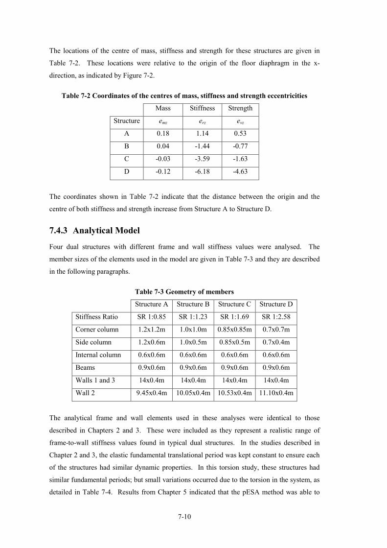
7�10

The locations of the centre of mass, stiffness and strength for these structures are given in

Table 7�2. These locations were relative to the origin of the floor diaphragm in the x�

direction, as indicated by Figure 7�2.

Table 7'2 Coordinates of the centres of mass, stiffness and strength eccentricities

Mass Stiffness Strength

Structure emz erz evz

A 0.18 1.14 0.53

B 0.04 �1.44 �0.77

C �0.03 �3.59 �1.63

D �0.12 �6.18 �4.63

The coordinates shown in Table 7�2 indicate that the distance between the origin and the

centre of both stiffness and strength increase from Structure A to Structure D.

7.4.3 Analytical Model

Four dual structures with different frame and wall stiffness values were analysed. The

member sizes of the elements used in the model are given in Table 7�3 and they are described

in the following paragraphs.

Table 7'3 Geometry of members

Structure A Structure B Structure C Structure D

Stiffness Ratio SR 1:0.85 SR 1:1.23 SR 1:1.69 SR 1:2.58

Corner column 1.2x1.2m 1.0x1.0m 0.85x0.85m 0.7x0.7m

Side column 1.2x0.6m 1.0x0.5m 0.85x0.5m 0.7x0.4m

Internal column 0.6x0.6m 0.6x0.6m 0.6x0.6m 0.6x0.6m

Beams 0.9x0.6m 0.9x0.6m 0.9x0.6m 0.9x0.6m

Walls 1 and 3 14x0.4m 14x0.4m 14x0.4m 14x0.4m

Wall 2 9.45x0.4m 10.05x0.4m 10.53x0.4m 11.10x0.4m

The analytical frame and wall elements used in these analyses were identical to those

described in Chapters 2 and 3. These were included as they represent a realistic range of

frame�to�wall stiffness values found in typical dual structures. In the studies described in

Chapter 2 and 3, the elastic fundamental translational period was kept constant to ensure each

of the structures had similar dynamic properties. In this torsion study, these structures had

similar fundamental periods; but small variations occurred due to the torsion in the system, as

detailed in Table 7�4. Results from Chapter 5 indicated that the pESA method was able to

7�11

satisfactory predict results for structures with different elastic fundamental periods, therefore

the elastic fundamental periods of the structures were not varied in this study.

Table 7'4 Elastic fundamental periods

Period (s)

Structure A 1.45

Structure B 1.45

Structure C 1.45

Structure D 1.46

The columns were modelled as reinforced concrete members with an axial force moment

interaction yield surface. The beam members were modelled using Giberson one components

elements without axial force moment interaction on flexural response. The hysteretic

behaviour of the beam and the column members was represented by the Revised Takada

hysteresis loop, which is available in RUAUMOKO (Carr, 2009d). The plastic hinge lengths

for the beams and columns were determined by the values presented in Priestley et al. (2007).

The effective stiffness of the beam column joints in the analytical model was accounted for by

using rigid end block factors of 0.4 times the beam depth for the columns and 0.4 times the

column depth for the beams. This value was kept constant thought the analyses. A sensitivity

study, described in Appendix A.1.3, was carried out to determine if this assumption affected

the results; it was found to have negligible affect.

Effective section properties were used in the analysis to allow for the reduction in stiffness of

the members due to flexural cracking. The effective section properties reported in New

Zealand Concrete Structures Standard NZS3101 (2006) were used.

The analytical model of the wall, which is described in Chapter 6, was used in the analyses.

The reinforcing steel and concrete hysteretic behaviour was modelled using the Dhakal steel

hysteresis model developed by Dhakal and Maekawa (2002a), (2002b) and the Brian Peng

Concrete hysteresis model, which was developed by Maekawa et al. (2003). The plastic

hinge length of the wall was made equivalent to the length of the wall resulting in a 45

degrees strut angle. The effective length of the reinforcing bars was made equal to the plastic

hinge length. The width of the diagonal strut was made equal to 0.55Lw. The shear

deformation parameters and the contact stress values were determined using the formulas

provided in the chapter on the wall element in Sections 6.3.5 and 6.3.6. The initial elastic

modulus for the concrete was 28GPa and for the steel was 200GPa. The compressive strength

of the concrete was 40MPa and the tensile strength was 3.8MPa

7�12

The floor diaphragm was modelled using elastic hybrid stress elements with 8 degrees of

freedom. The elastic modulus was taken as 28MPa with a Poisson’s ratio of 0.2. The floor

was modelled as a hollow�core floor with in�situ topping.

The foundation model was similar, but extended into 3�dimensions, to the foundation model

described in Section 3.1. The soil conditions in the analytical model represented shallow soil

conditions in the Wellington region, which relates to type C in the New Zealand Design

Actions Standard (Standards New Zealand, 2004a). Different soil conditions were considered

in Chapter 5 on the Floor Diaphragm Force Method, therefore only one soil type was included

in these analyses. The soil stiffness and strength parameters used for this foundation model

were the same as those detailed in Section 3.1.

The weight of the structures was applied at each of the node points in the structure. The

weights of the columns and walls were lumped proportionally to the nodes located above and

below the elements. The weights used to determine the floor forces were the same as these

detailed in Section 2.2.5.

7.4.4 Earthquake Records

The earthquake records used in the analyses are appropriate for the Wellington region. The

records were the North and South components of: El Centro, Lucerne, Izmit, La Union,

Llolleo and Tabas earthquakes. Additional details and the reasons of why these records were

chosen are given in Section 2.26.

These records were scaled according to the method provided in the New Zealand Structural

Design Actions Standard (Standards New Zealand, 2004a). The soil type assumed was

type C. The k1 scale factors used for each of the buildings modelled in this study are provided

in Table 7�5. The ground motion was applied along the z�direction, indicated by Figure 7�2.

Table 7'5 Earthquake record scale factors for z'direction loading

Record Direction k1

El Centro N 1.13

S 1.40

Lucerne N 0.77

S 1.72

Izmit N 1.61

7�13

S 1.40

La Union N 1.80

S 3.10

Llolleo N 1.27

S 0.71

Tabas N 0.45

S 0.58

7.4.5 pESA Method

The pESA method used in this study was performed by using the approach described in

Section 5.4. The parameters that were used are presented in the following paragraphs.

The fundamental periods used for the pESA method were the elastic fundamental periods

obtained from modal analyses, which are listed in Table 7�4 in Section 7.4.3. The modified

spectral shape factors, used to determine the pESA floor forces, were found from

Equation 5�20 in Section 5.4.3.2 for type C foundation soils.

Table 7'6 Structural ductility factors

Structural ductility factor

Structure A 2.1

Structure B 2.5

Structure C 2.3

Structure D 2.3

The strengths of the members used for this torsion study were determined by carrying out

time history analysis and checking that an acceptable response was obtained with respect to

the displacements and ductility capacities of members. The structural ductility factors,

required to determine the pESA method forces were obtained by determining the average

displacement ductility experienced by the frame and wall in the structure. The average

displacement ductility was obtained by averaging the displacement ductility for the frame and

wall for the range of earthquake records. The structural ductility factors that were used for

the pESA method are given in Table 7�6. Variations of the structural displacement ductility

were found by Castillo (2004) to have an insignificant affect on the displacements of

torsionally restrained structures. Therefore variations of the structural ductility were not

considered in these analyses.

7�14

The over�strength values, Øsb, of the lateral force resisting system required for the pESA

method were obtained from pushover analyses of the structures undertaken as part of this

research. These values are provided in Table 7�7.

Table 7'7 Over'strength values

Over�strength, Øsb

Structure A 2.4

Structure B 2.7

Structure C 2.2

Structure D 2.0

7.5 Results

The structural models A, B, C and D were analysed by inelastic time history and the pESA

methods. The results from inelastic time history analysis were assumed to provide the most

accurate estimate of the response. Comparisons were made between the predicted responses

to see how reliably the pESA method predicted inertial forces and the displacements at the

centre of mass. This was done to indirectly compare the ability of the pESA method to

predict the magnitudes of transfer forces. These comparisons were made to determine the

limitations of the pESA method with respect to torsionally susceptible structures.

The transfer forces, which develop in floor diaphragms, are related to the displacements of the

structure. In 3�dimensions, the magnitudes of transfer forces are expected to vary across floor

diaphragms. The forces are expected to be greatest between the vertical lateral force resisting

systems. For torsionally susceptible structures the displacements at the lateral force resisting

elements varies due to torsion. The displacements that were used in this study, to represent

the transfer forces in the floor diaphragm, were the values at the centre of mass parallel to the

orientation of the lateral force resisting elements. This displacement is indicated, in

Figure 7�3 by, �t, this represents the relative translational displacement of both lateral force

resisting systems.

7�15

X

Z

∆x

∆z

∆t

EQ

direction

Figure 7'3 Displacement of floor diaphragm subjected to torsion


Comparisons were made between the inertial forces predicted in the floor diaphragms by the

time history analysis and pESA methods. The inertial forces were obtained by multiplying

the accelerations at the centre of mass by the mass of the structure at the level being

considered. The averages of the peaks of inertial forces from the time history method were

used for these comparisons. Results presented in Chapter 2 and 3 indicated that inertial and

transfer forces, which contribute to the maximum total forces, do not necessarily occur

simultaneously. The magnitudes of transfer forces in the floor diaphragms were not obtained

for this torsion study due to limitations in the available modelling programs (this is a possible

area for future research). To determine the difference between using the maximum

combination inertial forces (from the maximum combination of total forces as was used in

Chapter 3) and the maximum inertial forces, ratios between these were obtained from the

results of the two dimensional transfer forces study that is described in Section 3.4.

7�16

0.0

0.2

0.4

0.6

0.8

1.0

1.2

0 10 20 30 40

Rati

o

Data number

Ratio between inertial forces for maximum

combination of forces and maximum inertial

forces

Figure 7'4 Ratio between inertial forces for the maximum combination of forces and the

maximum inertial forces

Figure 7�4 indicates the ratio of the maximum combination inertial force to the maximum

inertial forces for all of the levels of the 9�storey structures on soil D. This figure shows large

variations between the maximum combination of inertial forces and maximum inertial forces.

Ratio values of 1.0 in this figure indicate the maximum combination inertial force was equal

to the maximum inertial force. Ratios of less than 1.0 indicate the maximum combination of

inertial forces was less than the maximum inertial force. For this study, the maximum inertial

force values were used to ensure conservative comparisons between the pESA method and the

time history forces were made.

0 5000 10000

1

2

3

4

5

6

7

8

9

Force (kN)

Le

ve

l

Comparison between maximum

inertial forces from pESA and TH

methods for Structure A

TH

pESA

0 5000 10000

1

2

3

4

5

6

7

8

9

Force (kN)

Le

ve

l



methods for Structure B

TH

pESA

Figure 7'5 Comparison between maximum


methods for structure A



methods for structure B

7�17

0 5000 10000

1

2

3

4

5

6

7

8

9

Force (kN)

Le

ve

l



methods for Structure C

TH

pESA

0 5000 10000

1

2

3

4

5

6

7

8

9

Force (kN)

Le

ve

l



methods for Structure D

TH

pESA



methods for structure C



methods for structure D

Figure 7�5 to Figure 7�8 provides comparisons between inertial floor forces from time history

analyses and the pESA method. These results indicate that the pESA method provides a

conservative comparison to the time history results for Structures A and B for all levels and

Structure C for the upper levels. The floor diaphragm forces in the lower levels for Structure

C and D were underestimated by the pESA method. Levels 1 and 2 were underestimated by

20% and 10%, respectively for Structure C and Levels 1, 2, 3 and 4 were underestimated by

40% , 30%, 20% and 10% respectively for Structure D.

These comparisons indicated that with increasing torsional susceptibility (increasing from

Structure A to D) higher mode affects have a greater influence on the inertial forces at all

levels, but particularly at the lower levels of the structure. This is indicated by the poorer

representation of inertial forces by the pESA method, with increasing eccentricities, from

Structure A to D.

7.5.2 Displacements

Comparisons were made between the displacements at the centre of mass from time history

analyses and the pESA method to indicate the ability of the pESA method to predict the floor

diaphragm transfer forces.

As discussed in Section 7.5.1 for the inertial forces, the transfer forces were not obtained in

these analyses. Therefore the displacements which occurred when the combination of forces

were maximum were not obtained. To determine the differences between the displacements

7�18

for the maximum combination forces and the maximum displacements ratios between the

displacements were obtained.

0.0

0.2

0.4

0.6

0.8

1.0

1.2

0 10 20 30 40

Ra

tio

Data points

Ratio of displacements at maximum

combination of forces to the maximum

displacements

Figure 7'9 Ratio of displacements at maximum combination of forces to the maximum

displacements

Figure 7�9 shows the magnitude of the ratios between the displacements which occurred when

the combination of total floor forces were a maximum and the maximum displacements.

These results were from the analyses described in Section 3.4 for the all levels of the 9�storey

structures on soil type D. These results indicate that the majority of displacements for the

maximum combination of total forces were almost equal to the maximum displacements. On

the basis of the results shown in this figure, the average peak displacements were used to

represent the transfer forces from the time history analyses for each of the structures.

7�19

0.00 0.20 0.40

1

2

3

4

5

6

7

8

9

Displacement (m)

Le

ve

l


displacements from pESA and TH

results for Structure A

TH

pESA

0.00 0.20 0.40

1

2

3

4

5

6

7

8

9

Displacement (m)

Le

ve

l



results for Structure B

TH

pESA

Figure 7'10 Comparison between

maximum displacements from pESA and

TH results for Structure A



TH results for Structure B

0.00 0.20 0.40

1

2

3

4

5

6

7

8

9

Displacement (m)

Le

ve

l



results for Structure C

TH

pESA

0.00 0.20 0.40

1

2

3

4

5

6

7

8

9

Displacement (m)

Le

ve

l



results for Structure D

TH

pESA



TH results for Structure C



TH results for Structure D

Comparisons between the average peak displacements and the displacements obtained from

the pESA method are shown in Figure 7�10 to Figure 7�13. These figures indicate that the

displacements are very conservatively predicted by the pESA method. The pESA method can

not represent the reduction in displacements, which occurs in time history analysis, due to the

affects of rotational inertia in the floor diaphragm. This could provide a reason why the

pESA method provides a very conservative result.

7�20

7.6 Conclusions

The results from this torsion study indicate that the pESA method can satisfactorily predict

inertial forces for dual structures with frame�to�wall stiffness ratio of SR 1:1.23 (structure B).

Displacement comparisons indicate that the pESA method could conservatively predict the

displacements, and consequently the transfer forces, for structures with frame�to�wall stiffness

ratios of up to SR1:2.58 (structure D).

For Structure C and D the inertial forces were under predicted at the lower levels of the

structure by up to 40%. Displacement comparisons in the lower levels, for structures C and

D, indicated the pESA method predicts displacements of the order of two times the

displacements from time history analyses. The results from the study described in

Section 5.5.2.2 indicated that overestimating the displacements by a factor of two would lead

to twice the magnitude of transfer forces. Results providing comparisons between the

magnitudes of transfer and inertial forces, described in Chapter 2 and 3, indicate that the

magnitudes of transfer forces are typically greater than 40% of magnitude of inertial forces.

This would result in the total forces predicted by the pESA method for structure C and D

being conservative but the components of inertia and transfer forces being non�conservative.

From these results it is recommended that the pESA method be used for dual structures with

frame�to�wall stiffness ratios up to SR1:2.6.

7.7 References

Beyer, K. (2007). Seismic Desing of Torsionally Eccentric Buildings with RC U�Shaped

Walls. Rose School. Pavia, IUSS. Doctor of Philosophy.

Carr, A. J. (2009d). Ruaumoko Computer Program Library Christchurch, New Zealand,


Castillo, R. (2004). Seismic Design of Asymmetric Ductile Systems. Department of Civil

Engineering. Christchurch, University of Canterbury. Ph.D.

Dhakal, R. P. and Maekawa, K. (2002a). "Modeling for Postyield Buckling of

Reinforcement." Journal of Structural Engineering 128(9): 1139�1147.

Dhakal, R. P. and Maekawa, K. (2002b). "Reinforcement Stability and Fracture of Cover

Concrete in Reinforced Concrete Members." Journal of Structural Engineering

128(10): 1253�1262.

7�21

Maekawa, K., et al. (2003). Nonlinear Mechanics of Reinforced Concrete. London, Spon

Press.

Paulay, T. (1999). "A Simple Seismic Design Strategy Based on Displacement and Ductility

Compatibility." Earthquake Engineering and Engineering Seismology 1(1): 51�67.

Paulay, T. (2000). "Understanding Torsional Phenomena in Ductile Systems." Bulletin of the

New Zealand National Society for Earthquake Engineering 33(4): 403�420.

Paulay, T. (2001). "Some Design Principles Relevant to Torsional Phenomena in Ductile

Buildings." Journal of Earthquake Engineering 5(3): 273�308.

Priestley, M. J. N., et al. (2007). Displacement�Based Seismic Design of Structures. Pavia,

Italy, IUSS Press.

Priestley, M. J. N. and Kowalsky, M. J. (1998). "Aspects of Drift and Ductility Capacity of

Rectangular Cantilever Structural Walls." Bulletin of the New Zealand National

Society for Earthquake Engineering 31(2): 73�85.


New Zealand.

Standards New Zealand (2004b). Structural Design Actions Part 5 � Commentary. Wellington,

New Zealand, Standards New Zealand.



7�22

8�1

8 FORCE PATHS IN FLOOR DIAPHRAGMS

8.1 Introduction

The floor diaphragm of a structure provides a primary role in the performance of the structure.

It connects the elements (such as frames and walls) of the structure together to form a

structural system. It also transfers the forces which develop within the floor of the structure,

from dynamic affects such as wind or earthquake action, out to the vertical lateral forces

resisting elements of the structure. Careful design of the floor diaphragm is required to ensure

that admissible force paths can develop within the floor diaphragm and be transferred

successfully to the vertical lateral force resisting elements of the structure.

The majority of in�plane floor diaphragm design procedures that are available are based on

the assumption that the geometry of the floor is simple and regular. This assumption was

valid for the majority of structures built pre�1990s. Over the past decades the geometries of

floor diaphragms have change significantly resulting in previously employed floor diaphragm

design methods becoming obsolete. These changes have come about due to functional,

geometrical and architectural requirements of owners and clients. Complex floor diaphragms

include: irregular plan geometries of the floor diaphragm such as re�entrant corners, openings

or voids within the floor diaphragm to allow vertical traffic to move within the building and

floor diaphragms with different vertical lateral force resisting elements such as a combination

of frames and walls located asymmetrically around the structure. These irregularities can

cause force concentrations within the floor in zones such as, around re�entrant corners or

close to openings.

Limited guidance is currently available for designers on methodologies to design complex

floor diaphragms subjected to dynamic loadings. The New Zealand Concrete Structures

Standard (Standards New Zealand, 2006) suggests rational analysis, based on strut and tie

methods, should be used to ensure that admissible forces paths can develop within the floor

diaphragm. Limited verification has been carried out on the adequacy of using the strut and

tie methods to predict floor diaphragm forces.

In this chapter comparisons are made between analyses carried out using:

− Finite element analyses where the elements model cracking in concrete, elastic

behaviour of reinforcement, tension stiffening of concrete and non�linear response of

8�2

concrete in compression. This method of analysis is referred to as the inelastic finite

element method;

− Simplified finite element analyses where the concrete was assumed to be uncracked

and the reinforcement was assumed to be elastic. This method was referred to as

elastic finite element method;

− Strut and tie method.

The inelastic finite element method is assumed to provide the most reliable prediction of the

distribution of forces in floor diaphragms. Comparisons of the other methods were made to

this method.

The floor diaphragm layouts in this study included: variations of floor diaphragm geometries,

different locations of voids and penetrations within the floor, which represent lift shafts and

stair wells, and different layouts of vertical lateral force resisting elements such as walls.


8.2.1 Floor Diaphragm Design Methods

Descriptions of the design methods that are currently used to design floor diaphragm are

given in the following paragraphs. These methods include: the Beam Analogy method, the

Strut and Tie method, the Truss Analogy method and the Finite Element Analysis method.

These methods vary in the level of complexity and also in the level of accuracy that is

achieved.

8.2.1.1 Beam Analogy Method

The Beam Analogy method is a simple approach where the floor diaphragm is assumed to

behave like a simply supported deep beam. The loads are applied to the beam and the

moments and shear forces are calculated accordingly. Figure 8�1 provides a graphical

representation of a beam analogy design of a floor diaphragm.

8�3

Figure 8+1 Beam analogy for Diaphragm Design (NZCS, 1994)

This method is only suitable for the design of floors where the floor is not subjected to high

forces and the floor is reasonably regular in terms of geometry.

8.2.1.2 Strut and Tie Method

The Strut and Tie method is a more general approach than the beam analogy method. The

Strut and Tie method is carried out by assigning compression struts and tension ties

throughout the floor to develop a truss system of admissible force paths over the floor

diaphragm. This approach allows detailing of more complex floor layouts as the force paths

can be tracked for more irregular floor geometries. This method is appropriate for structures

where flexural and shear stresses are significant such as in buildings with long floors or

irregular floor layouts with voids and/or wings and re�entrant corners (Bull, 2004). An

example of a strut and tie solution, for a floor diaphragm, is provided in Figure 8�2.

Figure 8+2 Transfer of seismic forces through a concrete slab by the use of a Strut and

Tie solution (Bull, 2004)

Figure 8�2 shows the distribution of compression struts and tension ties for the Strut and Tie

method. The inertial forces which develop within the floor are equilibrated with compression

8�4

struts in the concrete and the tension ties in the steel to develop admissible force paths, around

obstructions such as openings, within the floor diaphragm. This diagram illustrates how the

strut and tie method can provide a much more detailed design compared to the beam analogy

method due to the greater detail of the method.

In general the strut and tie method is performed by subdividing the structural element into two

zones which represent two different types of deformation (Schlaich et al., 1987). The first

zone is known as the Bernoulli zone where strains vary linearly across a section as in standard

engineering flexural theory. The second zone is a disturbed region where engineering flexural

theory does not apply. The extent of a disturbed zone is determined by Saint Vénants

Principle, which states that the localised effects caused by any load acting on a body should

dissipate or smooth out within regions that are at a sufficiently distance from the irregularity.

These two regions are denoted as the B�region (beam or Bernoulli region) and the D�regions

(disturbed or discontinuous region). In the B�regions, the Bernoulli Hypothesis of plane

strain distributions can be assumed. The stresses can be easily derived from the forces within

these regions. The D�region denotes a disturbed or discontinuous region of internal forces,

where the strain distribution is non�linear. Such zones are associated with regions of

concentrated loads, openings and changes in geometry.

In many structural members different methods are used to determine the reinforcing layouts

for these two regions. The simple B�region can be designed using standard flexural theory

whereas the more complex D�region is generally designed with the load path or strut and tie

method (Schlaich et al., 1987).

In the case of floors diaphragms in buildings, there are no Bernoulli regions and the whole

floor needs to be designed as a disturbed strut and tie region. For any particular loading

situation, there are multiple possible strut and tie models. There are a number of requirements

for each solution:

− The load paths tend to take the shortest possible path with the least amount of strain

energy;

− Equilibrium of the struts and ties, at each node is maintained;

− The ties should be arranged using a practical reinforcement layout for the member;

− Struts (compression force paths) should not cross.

8.2.1.3 Finite Element Analysis

Inelastic finite element analysis methods can produce the most accurate representation of

floor forces. This method can be very time consuming and complicated. To carry out finite

8�5

element analyses, for a floor diaphragm, the floor is broken down into small elements which

allow the stress and strain actions within the floor to be calculated from the response of the

elements to the external loads. The size of the elements needs to be reduced until

convergence in predictions is obtained in successive analyses with reduced element sizes.

Finite element analyses allow the continuous nature of reinforced concrete floor diaphragms

to be modelled, unlike the Strut and Tie method which represents the floor diaphragm as

discrete elements. This allows the magnitudes of stresses around zones where stress

concentrations may be expected to occur, such as openings and re�entrant corners for

example, to be examined in detail.

Simplified finite element analyses, where the concrete is assumed to remain elastic, are

sometimes used for the design of floor diaphragms. The maximum and minimum principal

compression and tension forces in the concrete are identified from the analysis and

reinforcing steel is assigned to resist the principal tension forces. This is a much simpler

method in comparison to inelastic finite element analysis.

8.2.2 Requirements in New Zealand Standards and Codes

The design of reinforced concrete floor diaphragms in New Zealand is covered by two design

Standards: the New Zealand Loadings Standard (Standards New Zealand, 2004a) and the

New Zealand Concrete Structures Standard (Standards New Zealand, 2006). Both these

Standards recommend that floor diaphragms are to be designed to behave in an elastic manner

when distributing seismic forces to the lateral force resisting elements. “Elastic” in this

context refers to elastic behaviour for the majority of the floor away from the connections

between the floor and the supporting structure. The standard requires that the design is based

on rational analysis such as the strut and tie method.

When designing floor diaphragms by the use of the strut and tie method, the Standard requires

that the cyclic action and direction of a seismic event should be considered. The cyclic action

of a seismic event causes the external loads to change direction and hence change the load

paths of the internal forces acting in the diaphragm. Different sets of load paths should be

developed for seismic design of diaphragms ensuring all earthquake attack directions are

represented by the analysis.

The New Zealand Concrete Structures Standard requires the diaphragm is adequately

connected to the horizontal lateral load resisting elements to ensure there is sufficient capacity

to form admissible load paths throughout the structure and the deformations at the interfaces

8�6

to the supporting structure can be accommodated. The Standard also notes that penetrations

within floor diaphragms should be considered during the design of the floor diaphragm.

8.2.3 Past Research

8.2.3.1 Kolston and Buchanan

Kolston and Buchanan (1980) stated that floor diaphragms should be designed to perform

elastically to avoid affecting the behaviour of the primary vertical elements of the structure. It

is thought that the floor diaphragm may behave very poorly in the inelastic range due to the

slender shape and lack of detailing for inelastic behaviour.

The Reference stresses that care should be taken in the design of floor diaphragms with

openings. It was suggested that the location of openings should be positioned well away from

the edge of the floor diaphragm to ensure sufficient compression struts can form and therefore

allow adequate transfer of the compression forces between the lateral force resisting elements

and the floor.

8.2.3.2 Paulay and Priestley

Paulay and Priestley (1992) discussed issues involved with complex floor diaphragm layouts,

such as floors with: re�entrant corners, openings and irregular systems where torsional effects

about the vertical axis may develop. It was noted that re�entrant corners in floor diaphragms

may result in the development of stress concentrations at the re�entrant corner and lead to the

formation of severely damaged zones within the floor. It was suggested that seismic gaps,

which separate the structure into regular units, should be utilised to avoid the development of

these stress concentrations. This concept is illustrated in Figure 8�3 (a), (b) and (c).

Figure 8+3 Plan configuration in buildings (Paulay and Priestley, 1992)

8�7

Concerns were raised in Paulay and Priestley (1992) that openings or voids within floor

diaphragms, for lift shafts for example, may affect the ability of the floor to resist in�plan

shear and flexural force demands. It is suggested that openings should be located in a

symmetrical manner around the floor with either sufficient surrounding floor diaphragm, or

appropriate vertical lateral force resisting elements, to ensure the flexural and shear forces

demands are met. Examples of this are shown in Figure 8�3 (d) and (e). It is suggested in the

reference that most of the major problems associated with floor diaphragms can be minimised

by ensuring the design of the structure is symmetric.

8.2.3.3 Jensen

Research was carried out by Jensen (2004) on the distribution of forces predicted to develop

in a floor diaphragm using different design methods. The methods used were: elastic finite

element analysis, strut and tie analysis and the beam analogy method. The objective was to

assess the accuracy of the simpler methods.

The layout and geometry of the floor diaphragm that was used in most of Jensen’s analytical

studies was based on the size and dimensions of the floor diaphragm tested in a 3�dimensional

experimental study carried out by Matthews (2004) at the University of Canterbury. An

overview of the structure that was used in Matthews experimental testing is provided in

Section 8.2.4. A few other floor diaphragms with different geometric aspect ratios were also

included in Jensen’s study. Simple supports were provided in the direction of the applied load

but not in the direction perpendicular. This was done to allow tension forces to develop in

floor diaphragm. The applied forces were distributed at the nodes over the floor diaphragm.

The findings from this study are listed below:

− The horizontal beam analogy method was found to be adequate in predicting the

external reaction forces but it could not predict the internal stress flows within the

floor diaphragm;

− The strut and tie hand analysis method was found to compare well with the elastic

finite element results.

8.2.4 Cracking Patterns in Floor Diaphragms

Past experimental testing on floor diaphragms, carried out by Matthews (2004), Lindsay

(2004) and Blandón and Rodriguez (2005), showed that extensive cracking tended to develop

round structural elements that provided lateral force resistance.

8�8

The experimental work carried out by Matthews (2004) investigated the seismic performance

of precast hollow�core floors in a two�way moment resisting frame structure. The bay widths

were 6.1m and the columns were 750 by 750mm in size. The structure was tested under quasi

static cyclic loading where the structure was pushed through positive and negative drifts of

0.5%, 1.0%, 2.0% and 2.5%. Between each drift level the structure was unloaded. Research

carried out by Lindsay (2004) extended the work that was carried out by Matthews (2004).

The precast frames of Matthews (2004) testing were repaired, modified and used for

Lindsay’s testing. The crack patterns which developed in the Mathews and Lindsay tests are

shown in Figure 8�4 and Figure 8�5.

In the Matthews and Lindsay tests the lateral forces were applied to the South frame shown in

Figure 8�4 and Figure 8�5. The columns in the North frame were on rollers and consequently

this frame provided no lateral resistance. In the two tests the only diaphragm shear in the

floor was induced by incompatibility force effects due to the floor restraining elongation from

the plastic hinges which developed in the moment resisting frame (the south frame). The

forces simulate local inertia forces of the floor diaphragm.

The work carried out by Blandón and Rodriguez (2005) was based on an experimental study

of a half scale, two�storey precast concrete structure with a frame�to�wall structural system.

The crack pattern obtained from this experimental test is shown in the Figure 8�6. The lateral

forces, which represent the inertial forces, were applied to the floor at mid�span position

between the end walls. For practical purposes a concentrated lateral load force was applied,

which is different to in an earthquake where the inertial forces would be distributed across the

floor.

Figure 8+4 Cracks in the concrete topping of the floor diaphragm after the completion of

the +2.5% and +2.0% drift cycles from the experimental work of Matthews (2004)

8�9

South frame

Figure 8+5 Crack pattern of floor diaphragm at 5% drift along the infill from the

experimental work of Lindsay (2004)

Figure 8+6 Crack patterns observed in a reinforced concrete floor diaphragm of a dual

system at 3% drift from the experimental work of Blandón and Rodriguez (2005)

Figure 8�4 to Figure 8�6 show various crack patterns from laboratory experiments on cyclic

testing on floor diaphragms. Matthews (2004) full scale experimental results indicated that a

zone of extensive cracking extended in a near circular pattern with a diameter of around 1.5m

around the columns when subjected to 3% drift. A circular diameter of around 1.2m was

shown to form around the columns at a drift of 3% in the full scale experimental work of

Lindsay (2004). This distance related to the distance from the edge of the floor to the edge of

the timber infill between the perimeter beam and the first precast concrete floor unit which

was used in Lindsay’s experiment to ensure the hollow core floor acted as a one way floor

system. This arrangement is a common design feature used in newly constructed multi�storey

buildings.

8�10

Experimental work carried out by Blandón and Rodriguez (2005), on the half scale specimen,

found that the extensive crack pattern had a diameter of about 1m for the half scale building at

a global drift ratio of 3%. These tests indicate that the extensive zone of cracking, for cyclic

loading, is around 1m to 2m in size around columns. The cracks located around the wall of

this test were observed to develop at the slab to wall interface.

8.2.5 Modified Compression Field Theory

Modified compression field theory (Vecchio and Collins, 1986) is currently one of the most

sophisticated methods available for analytically modelling the behaviour of reinforced

concrete elements. Modified compression field theory is based on a smeared crack approach

which considers cracks at the integration points of the elements rather than tracks the

formation of large cracks which form over multiple elements. This method incorporates

equilibrium, compatibility and stress�strain relationships to describe the stress�strain

characteristics of each element. Average stresses and average strains of the reinforced

concrete elements are used for obtaining these stress�strain relationships.

The effects of localised stresses and strains are incorporated in the modified compression field

model to represent the transfer of loads across cracks. The following items are incorporated

in the modified compression field model to ensure that the integrity of the elements remains at

cracked locations:

− Change in tensile stress in the concrete (low across a crack and high between);

− The change in stress in the reinforcing steel (high across the crack and less between

cracks, see Figure 8�7a);

− Aggregate interlock (due to the cracking pattern in the concrete) across and along the

crack interface (shown in Figure 8�7b).

8�11

Cra

ck

Cra

ck

Tension in reinforcement

Tension in concrete

T

Elevation of floor

(a) Variation of stress in concrete and steel

across a crack

(b) Aggregate interlock across

a crack

Figure 8+7 Tension stiffening of concrete and shear transfer by aggregate interlock

Experimental testing has been carried out by various researchers (Vecchio and Collins (1986),

Mau and Hsu (1987) and Ang (1985)) to verify the accuracy of this method for analytical

modelling. The comparisons between experimental results and analytical results have been

found to provide good agreement for beam and walls subjected to shear, flexure and axial

load.

8.2.6 Summary of Literature Review

In recent decades, the geometry of floor diaphragms, in multi�storey structures have tended to

become more complex. Earlier design methods, based on simplifying assumptions, are not

applicable to the complex geometry of floor diaphragms that are frequently required today.

The research carried out by Jensen indicated that the Beam Analogy method was adequate at

predicting the reaction forces between the diaphragm and vertical structure. However, the

method was inadequate for describing the forces which develop within floor diaphragms. His

research also indicated that the strut and tie method provided comparable results to elastic

finite element results for floor diaphragms of varying length�to�width geometries, provided in

the strut and tie model was chosen with care.

The New Zealand Concrete Structures Standard NZS3101:2006 (Standards New Zealand,

2006) recommends the use of strut and tie methods to design and detail floor diaphragms.

Limited verification (Bull, 2004) has been carried out on the ability of this method to

8�12

adequately predict floor diaphragm forces. The accuracy of the strut and tie method is

considered in the next section of this report.

8.3 Description of Analysis

Inelastic finite element analytical models have been developed herein to allow the distribution

of forces, which develop in floor diaphragms due to lateral forces, to be tracked within the

floor diaphragm. A range of different floor diaphragm layouts are incorporated in this study

to determine how different floor diaphragm types affect the distribution of forces in the floor

diaphragm. The floor diaphragm layouts included are:

− Regular with varying length to width geometry;

− Irregular with re�entrant corners, such as L�shaped floors;

− Openings representing lift shafts and stairs;

− Different vertical lateral force resisting elements consisting of frames or walls.

The analytical models represent the in�plan behaviour of a floor diaphragm located at level 9

of a 9�storey building designed for a structural ductility of 3 in the Wellington region of

New Zealand. Static forces, determined from the pESA method, which are described in

Chapter 5, were applied to the floor diaphragm to represent the distribution of inertia forces.

A sensitivity study was carried out (reported on in Appendix D.2) to determine how the

distribution of forces, which developed in the floor, was affected by different applications of

lateral forces in the analyses. This study indicated that the best way to distribute the loads

was in proportion to the masses of the floor diaphragm at the individual nodes, where nodes

are the locations in the analytical model where the masses are lumped and the elements are

connected. The direction of the applied static forces to the floors was varied to ensure that a

range of possible earthquake attack directions were considered.

The analyses in this section are based on assessing diaphragm forces due to inertial actions

associated with the mass of the floor. Forces due to incompatibility self strain actions, which

developed due to differential displacements of the lateral force resisting elements, were not

considered. The buildings considered in this study were generally vertically regular with

lateral force resisting elements of either structural walls of the same length or moment

resisting frames. For these structures, diaphragm forces which are induced due to

deformation incompatibilities between the vertical lateral force resisting elements are

negligible, except for the forces associated with elongation of plastic hinge zones which is

outside the scope of this study.

8�13

Some of the floor layouts, described in Section 8.3.1, have irregular vertical lateral force

resisting systems which could develop torsional response. Static analyses overestimate the

rotation of a floor diaphragm of torsionally susceptible buildings due to static methods

neglecting the mass rotational moment of inertia (as observed in Chapter 7). Neglecting this

should not affect the results of this section as the results are primarily focused on the trends of

the forces rather than the absolute magnitudes. Further to this, variations in the rotation of the

structure could occur due to different orientations of earthquake loading and for different

member stiffness values.

The floor system, represented in the analytical models is based on a hollow�core flooring

system with a depth of 300mm and a concrete topping of 75mm. A constant floor thickness

was used in all of the models described in this chapter. Analyses, described in Appendix D.4,

using different floor thicknesses indicated that the thickness of the floor did not significantly

affect the flow of forces in the floor diaphragm.

8.3.1 Floor Layouts

Analyses were carried out on all of the floor layouts, described in the following sections, for

earthquake directions at 45 degree increments around the structure to ensure the possible load

paths that could eventuate from an earthquake were considered. In the case where symmetry

of the floor layouts exists, some of the loading orientations were omitted to avoid repeating

results. The size and stiffness of the members used in these models are described in

Section 8.3.4.

8.3.1.1 Different Rectangular Geometries

Three different geometric length�to�width ratios of floor diaphragms were investigated.

These ratios are typical of geometries of buildings constructed in New Zealand. The length�

to�width ratios of the floors that were used in this study are provided in Table 8�1 below.

Table 8+1 Investigated floor geometries

Floor Ratio Geometry

1 1:2 14x28m

2 1:1 28x28m

3 2:1 28x14m

The seismic system for these floors is a seismic perimeter frame with internal vertical load

resisting frames. The width of the bays for these floors is 7m, the sizes of the columns and

8�14

beams used in these floors are described in Section 8.3.4. Figure 8�8 provides a plan view of

the floor diaphragms.

Geometric ratio of 1 to 2

0m

7m

14m

21m

28m

0m 7m 14m 0m 7m 14m 21m 28m 0m 7m 14m 21m 28mX

Y

0m

7m

14m

21m

28m

Y

0m

7m

14m

Y

X X

Geometric ratio of 1 to 1 Geometric ratio of 2 to 1

Figure 8+8 Plan view of the floor diaphragms

8.3.1.2 Irregular Plan Geometry

L, U and T structures were investigated to determine the affects of re�entrant corners on the

distribution of forces which flow through floor diaphragms. Structures with re�entrant

corners have been found by past researchers to develop large stress concentrations at the

location of the re�entrant corner of the floor. Figure 8�9 provides a plan view of the geometry

of the floor diaphragms.

8�15

7m

0m

14m

21m

28m

7m0m

14

m

21m

28m

7m

0m

14m

21m

28m

7m0m

14m

21

m

28m

35m

7m

0m

14m

21m

28m

7m0m

14m

21

m

28

m

Y

X X

Y

Y

X

Re�entrant corner

Figure 8+9 Different geometric shapes used in the analysis of floors with re+entrant

corners

The structural system of these floors consisted of frames which were to resist both vertical

and lateral forces. The wings of the L�shaped structure are 28m long and 14m wide and the

bay lengths spanned 7m. The U�shaped structure is 28m long and 35m wide with 7m wide

bay lengths. The T�shaped structure is 28m high and 28m wide, with a width and the length

of the base of the T is 14m.

8.3.1.3 Openings in the Floor Diaphragm

Openings, voids and penetrations of various sizes exist in floor diaphragms to allow for

vertical traffic, such as people, vehicles and electrical services, to move vertically within a

building. The presence of openings can affect the flow of forces through floor diaphragms

and cause stress concentrations near the openings.

8�16

The typical size of floor space required to construct a lift shaft is 2.5m by 2.5m and the size

for a stair�wells is typically 2.5m by 5 to 6m. The combination of one stair well and two lift

shafts, which is a common combination used in New Zealand buildings, was used to model

the openings in this study. For this combination of lifts and stairs, an opening size of 7m by

7m, which is equivalent to one bay width for the buildings used in this study, was used. This

size is slightly larger than the size required for the two lifts and one stair well, but additional

space is typically required for mechanical and electrical services. The geometric dimension

of the floor diaphragm used in this study was 28m by 28m.

Opening

X

Y

Figure 8+10 Model used in the study of floor diaphragms with openings

A beneficial study would be to determine whether it is acceptable to ignore the effects of

small openings such as those for electrical services in the design process; this is beyond the

scope of this research. To determine the affects of openings, considerations must be given to

the: size of the opening, the location of the opening within the floor diaphragm, the

reinforcing steel within the floor and the shape of the floor diaphragm.

8.3.1.4 Walls for Lateral Force Resisting System

Analyses were carried out on a variety of floors with different wall arrangements to determine

how walls in different locations, around a floor diaphragm, influence the distributions and

magnitudes of floor forces. The floors investigated in this section consisted of walls on three

sides of the structure. This type of wall layout is common for buildings that have a street

frontage. The generalised layout of the location of the walls around the floor diaphragms that

are used in this study are shown in Figure 8�11.

8�17

0 147 21 28m

X

Wall A

Wall C

Wall B

014

72

12

8m

Y

Figure 8+11 Typical wall layout for open front structures used in this study

The labels Wall A, B and C in this figure indicate the location of the walls that are referred to

in Table 8�2. The length and location of each of these walls for the different floor layouts

included in this study are provided in the table. These layouts provide a reasonable

representation of the length and layout of reinforced concrete wall structures that are typically

constructed in New Zealand.

Table 8+2 Length and location of walls around the floor diaphragms

Floor layout

Wall A (m)

Location of wall A

Wall B (m)

Location of wall B

Wall C (m)

Location of wall C

1 7 y: 14�21m 14 x:7�21m 7 y: 14�21m

2 14 y:14�28m 14 x:7�21m 14 y:14�28m

3 7 y: 7�14m 28 x:0�28m 7 y: 7�14m

4 7 y: 14�21m 28 x:0�28m 7 y: 14�21m

8.3.2 Analytical Floor Diaphragm Model

Two possible elements were available to represent the floor diaphragm in the analysis. These

elements were the lattice element available in RUAUMOKO (Carr, 1981�2009b) and inelastic

finite elements available in ABAQUS (ABAQUS, 2004a).

The lattice element is based on the Hrenikoff lattice analogy and the lattice framework which

was presented in the early 1940s (Hrennikoff, 1941). This element provides a simple

8�18

alternative compared to modelling a continuous material, such as in finite elements as the

lattice element represents a continuum by discrete elements. In the analytical modelling

program RUAUMOKO, this element is represented by four nodes with six adjoining spring

members joined together in a lattice formation with four perimeter members and two diagonal

members configured in a chosen geometry which is fixed for the analysis, as shown in

Figure 8�12.

Figure 8+12 Lattice truss element (Carr, 1981+2009b)

A study was carried out to determine whether the lattice element could adequately represent

the distribution of force in the floor diaphragm. The results from this study indicated that the

fixed geometry of the struts affect both the magnitudes and the orientation of the forces in the

floor diaphragm. A detailed description of the lattice element is provided in Appendix D.1.1

including how the principle stresses were obtained. Comparisons between lattice element

results and finite element results are provided in Appendix A.1.3. As a consequence, inelastic

finite elements were used in the analyses of the floor diaphragms.

The model used to represent the reinforced concrete floor diaphragm consisted of two, two�

dimensional four node shell finite elements, which represented the concrete and the steel

reinforcing components of the floor. These two material layers were artificially separated to

allow the average forces which developed in each material, to be separately identified. Strain

compatibility between the two materials was maintained. The finite element mesh type, used

for both materials, was an iso�parametric quadrilateral mesh. The finite element mesh size

that was used for this study was 1m by 1m. A succession of inelastic finite element analysis

was made using different sized elements. It was found that a mesh size of 1m by 1m gave

convergence of predicted actions with smaller mesh sizes. Details of this study are provided

in Appendix D.3.

8�19

8.3.3 Analytical Modelling Problems

When developing the analytical model, for this study, some analytical modelling problems

arose due to issues associated with singularities in the analyses. The columns in the analytical

models were initially represented by singular points. This caused stress concentrations to

develop at the column nodes. A simple study was carried out to determine if this problem

could be avoided by representing the width of the columns in the analytical model rather than

representing the columns by a singular node. The results indicated that incorporating the

width of the columns in the analytical model removed the singularity problem. The results

from this study are provided in Appendix D.7.

Another analytical modelling problem, which was observed in the initial results, was the

development of singularities in the floor diaphragm associated with changes of the floor

diaphragm geometry. A number of different methods to deal with this problem were

considered in Appendix D.8. The method that was used was based on an approach suggested

in ABAQUS (2004b). This method requires the region of the singularity to be excluded from

the re�meshing process by partitioning the area around the singularity and obtaining

convergence for the remaining region of the floor diaphragm.

8.3.4 Member Size and Stiffness

The sizes of the columns, beams and walls used in the models are provided in Table 8�3.

“Gravity columns”in this table refer to the columns which only resist vertical loads. The

length of the walls used in the different models was varied depending on what was being

investigated. The specific lengths of the walls that were used for the floors with walls

analytical models are provided in Section 8.3.1.4.

Table 8+3 Dimensions of the column members

Corner columns 1.0x1.0m

Exterior columns 1.0x0.5m

Gravity columns 0.6x0.6m

All Beams 0.9x0.6m

Walls 0.4xAm

The various lengths of the walls used in this study, indicated by parameter A in Table 8.3, are

provided in Table 8�2. The stiffness assigned to the lateral force resisting elements was based

on the gross section stiffness times a factor to allow for the reduction in stiffness due to

cracking. The factors used for this are from the Concrete Structures Standard (Standards New

8�20

Zealand, 2006). The geometry of the wall members included in this study correlate to walls

that are typically flexural dominated. The shear deformations were assumed to be negligible.

A study, described in Appendix D.6, was carried out to determine the values to use in these

analytical models for the relative stiffness of the out�of�plane deforming exterior columns and

interior columns which only resist vertical loads. This study indicated that in the strong

direction of the floor, which is parallel to the direction of the floor beams, the weak direction

exterior columns should have a stiffness of 54% of the effective cracked column stiffness and

the gravity columns should have a stiffness of 48% of the effective cracked column stiffness.

For the weak direction of the floor, which is the direction perpendicular to the floor beams,

both the weak direction exterior columns and the columns which resist only vertical loads

were observed to have negligible stiffness contribution and therefore for this direction the

stiffness of these columns was neglected in the analytical models. Further details regarding

this study are provided in Appendix D.6.

8.3.5 Material Model

8.3.5.1 Concrete

Various material models are available to represent the behaviour of reinforced concrete.

These models vary in complexity ranging from representing the macro behaviour which

includes basic yielding of the reinforcement to micro behaviour such as modelling the

orientation of cracks, opening and closing of cracks, tension stiffening effects of reinforced

concrete, local stresses in reinforcing bars at cracks and shear and compression transfer across

cracked concrete.

Two concrete material models are available in ABAQUS (2004a); these are the smeared

cracking concrete model and the concrete damage plasticity model. A description of each of

these is provided in the following paragraphs.

The concrete damage plasticity model is a continuum, plasticity�based, damage model. The

inelastic response of the concrete is based on the concepts of isotropic damage elasticity along

with isotropic tensile and compressive plasticity (ABAQUS, 2004b). This model assumes

two main failure mechanisms; tensile cracking and compressive crushing of the concrete

material. The concrete damage plasticity model is a simpler model in comparison to the

smeared cracking model as it is based on isotropic damage plasticity. In reality, as plasticity

forms in a concrete member, the response becomes orthotropic (Lee and Willam, 1997). This

8�21

model does not incorporate any micro affects, such as the affects of additional shear stiffness

due to aggregate interlock when a crack forms.

The concrete smeared cracking model, available in ABAQUS (2004a), is intended for

modelling reinforced concrete members subjected to monotonic loading conditions. It is

based on modified compression field theory (Vecchio and Collins, 1986). The concrete is

assumed to behave isotropically to the point of cracking, once cracking has occurred the

material is then assumed to behave orthotropically (ABAQUS, 2004b). Average stresses and

strains for each finite element are used for the calculations of the response of each element.

The use of average stresses and strains conceal the large stresses which can develop in

reinforcement at cracks in concrete. This occurs in the intermediate phase between when the

section is elastic and when the section is fully cracked. For the uncracked and fully cracked

cases, peak forces (not average forces) are reported.

A simple study was carried out to determine the ratio between peak stresses at the cracks and

average stresses provided by the concrete model. The analytical model used for this study

was a 40m by 10m element with tension forces applied down the shorter side; this model is

shown in Figure 8�13. This model used similar elements to the elements used to represent the

floor diaphragms.

Figure 8+13 Analytical model for simple peak to average stress study

The model was loaded until it was fully cracked so the concrete provided very little tensile

capacity. For the intermediate case where some cracks had developed, average stresses in the

concrete were recorded. For this case, the magnitudes of the concrete and steel for different

stages of cracking were obtained from the results and compared to the total expected force to

determine the ratio between the average stress and the peak stress. For different stages of

cracking the ratio of the peak to average forces varies. The maximum peak to average ratio

was found to be 1.4.

In the smeared cracking model, the effects of tension stiffening and shear retention are

considered. Shear retention represents the additional shear stiffness which exists in a cracked

element as a result of aggregate interlock between adjacent surfaces of concrete either side of

8�22

a crack. The inclusion of tension stiffening in the model helps to represent the interactions

between the reinforcing bar and the concrete such as bond slip and dowel action. Tension

stiffening effects can be modelled using either a stress�strain relation or a fracture energy

criterion.

When a crack develops with this smeared concrete material model (described in Section

8.3.2) the orientation of the crack is fixed. A fixed crack orientation is appropriate for this

model as this model is monotonically loaded. If the orientation of cracks in a floor diaphragm

due to cyclic loading was to be analytically modelled, a different concrete material model

would be required.

For the concrete isotropic elastic behaviour a Young’s modulus of 30GPa and a Poisons ratio

of 0.2 was assumed. The yielding compressive stress of the concrete was taken as 40MPa.

Tension stiffening effects were incorporated into the model.

The strength of concrete in tension is variable and localised cracking may occur due to

shrinkage, differential temperature and gravity loading for some examples. As a result,

design reinforcement is provided to resist the total tension forces, which in terms of the model

corresponds to the average tension force in the reinforcement plus the average component of

tension force in the direction of the reinforcement. For this research, it is of interest to

determine how cracking in the floor diaphragm affects the distribution of the forces paths.

This affect is investigated by repeating the same analysis with different tensile strengths of

concrete.

The New Zealand Concrete Structures Standard NZS3101:2006 (Standards New Zealand,

2006) suggests that the indirect tensile strength for normal density concrete is of the order of

0.36√f’c. For a concrete with compressive strength of 40MPa, as used in these studies, the

modulus of rupture should be taken as 2.3MPa. This leads to a concrete tension�to�

compression failure ratio of around 0.1. A further tension�to�compression ratio of 0.002 was

used to represent the case where significant cracking in the concrete occurred. Zero concrete

tension strength could not be used in this analytical model. For this study tension�to�

compression failure ratio of 0.1 and 0.002 were employed to represent the two cases tension

capacity in the concrete.

In this research the affects of a range of different concrete tensile strengths on the distribution

of floor diaphragm forces were considered. To determine the affects, floor force distribution

patterns were developed for floors with different concrete tension�to�compression strength

8�23

failure ratios (FR). The concrete tensile to compressive strength failure ratios that were

included for each of the floor layouts were:

− FR of 0.1 which represented no or limited cracking of the concrete over the whole

floor diaphragm;

− FR of 0.002 which represented significant cracking of the concrete over the whole

floor diaphragm;

− FR of 0.002 for 1m around the vertical lateral force resisting elements and FR of 0.1

over the rest of the floor;

− FR of 0.002 for 2m around the vertical lateral force resisting elements and FR 0.1

over the rest of the floor.

The floor diaphragms analytical models which had significant cracking over 1m or 2m

distance around the vertical lateral force resisting elements represented similar cracking

patterns observed in tests of floor diaphragms (Matthews (2004), Lindsay (2004), and

Blandon and Rodriguez (2005)). A description of the experimental tests and cracking patterns

is provided in the literature review in Section 8.2.4. Analytical models of both 1m and 2m

cracking regions were developed to determine the sensitivity the size of the cracking region in

Section 8.4.1.

8.3.5.2 Steel

The reinforcing used in the analytical floor diaphragm models was assumed to be D12

reinforcing bars. Reinforcing mesh was not used in the analytical floor diaphragm model due

past results from experimental tests which indicated poor performance (Matthews (2004) and

Lindsay (2004)) of the reinforcing mesh. The steel material in these analytical models was

assumed to remain elastic, with an elastic modulus of 200GPa and the Poisons ratio used

was 0.3.

The reinforcement in the floor diaphragm was represented in the model by a smeared layer of

steel with axial stiffness in the longitudinal and transverse directions and no shear stiffness.

This smeared layer approach was employed to avoided complications associated with finite

element mesh sensitivities due to the size and location of the reinforcement within the floor.

This modelling representation is realistic as the reinforcing bars are typically closely spaced.

A sensitivity study was carried out, which is described in Appendix D.9, to investigate if the

smeared layer of steel representation verses the individual bars representation of the

reinforcing steel mesh affected the distribution of the forces which developed in the floor

diaphragm. The results from this study indicated that there was little difference in the

distribution of the forces.

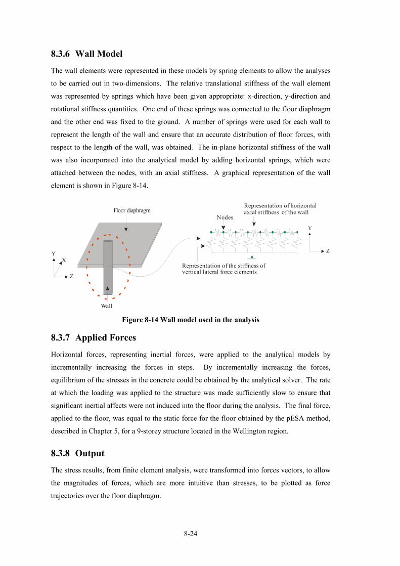
8�24

8.3.6 Wall Model

The wall elements were represented in these models by spring elements to allow the analyses

to be carried out in two�dimensions. The relative translational stiffness of the wall element

was represented by springs which have been given appropriate: x�direction, y�direction and

rotational stiffness quantities. One end of these springs was connected to the floor diaphragm

and the other end was fixed to the ground. A number of springs were used for each wall to

represent the length of the wall and ensure that an accurate distribution of floor forces, with

respect to the length of the wall, was obtained. The in�plane horizontal stiffness of the wall

was also incorporated into the analytical model by adding horizontal springs, which were

attached between the nodes, with an axial stiffness. A graphical representation of the wall

element is shown in Figure 8�14.

Floor diaphragm

Wall

Nodes

Representation of the stiffness of vertical lateral force elements

Representation of horizontal axial stiffness of the wall

YX

Z

Y

Z

Figure 8+14 Wall model used in the analysis

8.3.7 Applied Forces

Horizontal forces, representing inertial forces, were applied to the analytical models by

incrementally increasing the forces in steps. By incrementally increasing the forces,

equilibrium of the stresses in the concrete could be obtained by the analytical solver. The rate

at which the loading was applied to the structure was made sufficiently slow to ensure that

significant inertial affects were not induced into the floor during the analysis. The final force,

applied to the floor, was equal to the static force for the floor obtained by the pESA method,

described in Chapter 5, for a 9�storey structure located in the Wellington region.

8.3.8 Output

The stress results, from finite element analysis, were transformed into forces vectors, to allow

the magnitudes of forces, which are more intuitive than stresses, to be plotted as force

trajectories over the floor diaphragm.

8�25

Principal stress values can be directly obtained from the ABAQUS (2004a) output. The

orientation and components for each orientation, of these principal stresses can not be easily

obtained though. Therefore, the values for the force trajectories were obtained by converting

the normal and shear stresses for each finite element, into principle stresses for each finite

element. This was done using the same procedure as described for the Lattice Element in

Appendix D.1.1.3. During this conversion the orientation and the x and y�components of the

forces were obtained.

Width

Width

Principal stress

Figure 8+15 Width of principal stress values in finite element analysis

The principal stresses that were obtained during this process were cross checked with the

principal stress values obtained from ABAQUS (2004) to verify the hand method used to

calculate the principal stresses. To transform these stress values, into force values, the width

of the principal force vectors were determined with consideration of the angle of the force

vector fore each finite element. This is graphically represented by Figure 8�15. Care was

taken to ensure that the correct principle force angle was used, with the correct width, to

obtain the force vector. This width was multiplied by the thickness of the floor diaphragm to

obtain the force vectors.

8.3.9 Strut and Tie Analysis

Simple strut and tie models, similar to those typically used in design offices, were constructed

in this study to determine how accurate the strut and tie method is in comparison to the

inelastic finite element method.

8�26

This strut and tie model consists of a grillage of longitudinal, transverse and diagonal truss

members. The diagonal 45 degree angled truss members only resisted compression forces as

the assumption that the concrete had no tensile capacity was made for these models. The

axial stiffness of the truss members for the simple truss models were made to be equivalent to

the stiffness of the members for the finite element model. The analytical strut and tie model

was analysed using the static analysis program QSE (Research Engineers Ltd, 1999).

8.4 Results

A number of trends relating to the distributions and magnitudes of in�plane floor forces, for a

range of different floor diaphragms layouts, were investigated. This included investigations

on:

− The sensitivity of the tensile capacity of concrete;

− Comparisons between inelastic finite element results and strut and tie results.

Comments were provided on possible reinforcement details to minimise the affects of

significant cracking over zones were redistribution of forces are expected to occur;

− Comparisons between the inelastic finite element results to elastic finite element

results;

− The trends of the angles of the concrete forces both at the interface between the

lateral force resisting elements and in the general region of the floor diaphragm away

from the lateral force resisting elements;

− The geometry of the forces at the interface between the lateral force resisting

elements and the floor diaphragm (at the nodes);

− The distribution of compression and tension forces at the interface of walls.

Discussions of these trends are provided in the following paragraphs. It should be noted that,

for the following figures, the reactions with the interior columns are not shown.

Results and comments on the general trends of forces which develop in floor diaphragms are

provided for a selection of the floor layouts in the following Sections. The results for the rest

of the floor layouts considered in the study are provided in Appendix D.10. Appendix D.10.1

provides general trends for floor diaphragms of different geometry including; L, U, T�shaped

floors, floors with openings, L�shaped floors with openings and floors with walls as the lateral

force resisting system.

8.4.1 Tensile Capacity of Concrete

Floor force distributions for each of the different floor layouts, with different concrete tensile

to compressive strength failure ratios, were developed to determine how the concrete tensile

8�27

capacity affected the force distribution within the floor plate. Comparisons between the force

distributions indicated how the change in stiffness due to cracking affected the distribution of

forces. The results for the regular floor diaphragm of 28m by 28m load monotonically in the

y�direction as indicated by the key are shown in Figure 8�16 to Figure 8�19. The angles for

these force trajectories are provided in Figure 8�31 and Figure 8�32 located in Section 8.4.5.

The results for regions in the floor with concrete tension�to�compression failure ratio FR of

0.1 were found to remain elastic for all of the floors. This indicates that the reported results

represent peak total forces and not a combination of peak steel forces and average concrete

forces. This is because the forces from the smeared concrete material model, when cracking

has occurred are average forces and not the peak forces at the crack location.

241K

N

220K

N

175KN179KN

142KN157KN

129KN108KN

61KN

39KN

28KN

12KN

36kN

45KN

89KN

129KN100K

N103KN

80KN

53KN

141KN

183KN

175KN

67KN

108KN

124KN

110kN97KN

76KN

95KN

103KN

121KN

131KN

104KN

30KN

109KN

127kN

120KN

103kN

111kN

49KN

79KN

24KN18

6K

N

24KN

67KN

103K

N

111KN

49KN

95KN

127K

N

76KN

120K

N

109K

N

30KN

104KN

131K

N

121K

N10

3KN

97KN

124K

N

108K

N

67KN

53KN

36KN

12KN

80KN

103K

N

129K

N

141K

N

183K

N

175K

N17

9KN

186K

N

157K

N

129K

N

100K

N

89KN

45KN

28KN

39KN

61KN

108K

N

142K

N

175K

N

220KN

241K

N

110K

N

116kN

94kN

129kN

78KN

44KN

21KN

8KN

44KN

78KN

129KN

94KN

116KN

21KN

8KN

8KN

8KN

275

KN

46kN

43

KN

43K

N46

KN

275kN

55KN

29

KN

29K

N

35KN547KN

272KN

547KN

272KN

272KN

Region 1 Region 1

Region 3

Region 2Region 2

306K

N

238K

N

201KN179KN

166KN140KN

108KN110K

N

72KN

30KN

17KN

9KN

13KN

33KN

57KN

138KN76K

N110K

N

64KN

29KN

160KN

188KN

154KN

139KN

152KN

126KN

116kN90KN

29KN

72KN

114KN

143KN

163KN

95KN

117KN

145KN

108kN

138KN

178kN

170kN

91KN

141KN

72KN18

8K

N

30KN

54KN

135KN

103K

N

27KN

60KN

83KN

55KN

106K

N

114K

N

70KN

29KN

80KN

83KN

73KN

68KN

82KN

77KN

93KN

57KN

75KN

80KN

61KN

70KN

75KN

89KN

89KN

29KN

174K

N

236K

N

152K

N

106K

N

85KN

68KN

73KN

77KN

75KN

99KN

103K

N

134K

N

155K

N

118K

N66K

N

84KN

217kN

120kN

70kN

20KN

12KN

6KN

8KN

30KN

46KN

79KN

148KN

126KN

13KN

10KN

9KN

1KN

59KN

81KN

440

KN

121

kN

25

7K

N8

2K

N4K

N2

26kN

13

6K

N3

KN

547KN

272KN

547KN

272KN

272KN

148

KN42KN

26kN

38KN

48KN

15KN

19KN

Region 3

Tension in concrete Compression in concreteCompression in steelTension in steel

KEY:EQ X

Y

Figure 8+16 Inelastic finite element force

trajectories for the 28m by 28m floor

loaded along the y+axis with a FR of 0.1


trajectories for the 28m by 28m floor

loaded along the y+axis with a FR of 0.002

8�28

Figure 8�16 and Figure 8�17 provide the internal floor force trajectories that were extracted

from the finite element analysis results by the method described in Section 8.3.8. Double

arrows shown in this figure indicate that tensions or compressions from both concrete and

steel are present; the indicated force for this case represents the total force present in both

materials. The angles of the compression struts and tension ties of the concrete at each of the

columns are provided in Section 8.4.5. Figure 8�16 shows the floor force distribution for a

floor where very little cracking was assumed to occur with a tension�to�compression FR of

0.1 and Figure 8�17 shows the distribution of forces for a floor where significant cracking of

the concrete was assumed with a tension�to�compression FR 0.002. The general solution

shown in these floor diaphragms indicates that the floor is acting partially like a tied arch.

Comparisons between the relative magnitudes and distributions of the forces in both of these

floors indicate that the magnitude and distribution of the internal forces are reasonably

sensitive to the tensile capacity of the concrete. The magnitude of forces differs between

these floors due to the development of cracking in the concrete. The cracking caused the

force path to change significantly at the bottom corners of the floor (indicated by region 1 in

the figures). The change of force path was from a diagonal tension tie in the concrete at the

corner column, for the un�cracked floor, to lateral and transverse tension ties in the

reinforcing steel of the floors at the same corner, for the highly cracked floor. The magnitude

of the total tension tie forces in the y�direction in region 1, for the floor with the tension�to�

compression concrete FR of 0.1, was 509kN compared to the floor with the tension�to�

compression concrete FR of 0.002 was a tension value of 499kN. The largest notable

differences between these two cases is associated with the tension forces in the reinforcing

steel with a change from 275kN for FR of 0.1 to 440kN for FR of 0.002. This indicates the

increase in the forces transferred by the reinforcement due to the development of tension

cracking within the concrete.

The magnitude of the total tension and compression forces in the x�direction indicated by

regions 2 and 3 respectively in the figures differ for these floors with different tension�to�

compression failure ratios. The magnitudes of the x�direction total tension forces in region 2

of the floor, with a FR of 0.1, are shown to be 485kN and for the floor with FR of 0.002

419kN. This indicates that the elastic, FR of 0.1, case provides a conservative representation

of the forces.

The magnitudes of the x�direction total tension forces in region 3 of the floor were 55kN for

FR of 0.1 compared to 81kN for FR0.002. This indicates that the elastic solution

underestimates the results from the significantly cracked region.

8�29

Region 2Region 2

257K

N

220

KN

153KN172K

N

117KN147KN

121KN

81KN

42KN

28KN

16KN

10KN

32KN

40KN

77KN

105KN

117KN80KN

66KN

59KN

147KN

191KN

201KN

111KN

115KN

113KN

112kN

98KN

76KN

92KN

110KN

117KN

125KN

122KN

88KN

87KN

116kN

85KN

118kN

136kN

94KN

101KN

51KN

185K

N

21KN

40KN

79KN

108KN

28KN

85KN

149K

N

94KN

125K

N

90KN

26KN

30KN

94KN

109K

N10

1KN

115K

N

134K

N

120K

N

89KN

83KN

54KN

21KN

95KN

119K

N

126K

N

129K

N

101K

N

37KN

336K

N

369K

N

285K

N

211K

N

150K

N

101K

N70

KN

29KN

46KN

60KN

82KN

103K

N

88KN

100K

N

71

KN

125K

N

140KN

107KN

112KN

70KN

37KN

15KN

10KN

64KN

73KN

153KN

76KN

91KN

29KN

15KN

8KN

11KN

450K

N11kN

147

KN

10

4K

N67K

N26

7kN

28KN

52KN

35KN

17KN

7KN

62K

N49

KN

255K

N

177

KN

128KN247K

N

114KN174KN

135KN

105KN

81KN

63KN

36KN

20KN

46KN

64KN

77KN

119KN114KN

110KN

79KN51KN

142KN

173KN

188KN

106KN

129KN

118KN

109kN98K

N

81KN

99KN

110KN

124KN

137KN

120KN

48KN

78KN

129kN

100KN

95kN

133kN

83KN

100KN

27KN

168K

N

29KN

68KN

92KN

114K

N

27KN

94KN

130K

N

86KN

118K

N

92KN

25KN

25KN

84KN

106K

N10

2KN

109K

N

140K

N

137K

N

112K

N

68KN

40KN

13KN

89KN

110K

N

114K

N

123K

N

85KN

32KN

335K

N

363K

N

263K

N

191K

N

138K

N

83KN

56KN

27KN

48KN

69KN

96KN

118K

N

104K

N

106K

N

66

KN

123K

N

128KN

99KN

129KN

74KN

44KN

20KN

15KN

54KN

84KN

129KN

95KN

116KN

19KN

12KN

9KN

5KN

428K

N9

k N140

KN

89

KN

50K

N25

6kN

26KN

48KN

16KN

7KN

53K

N5

5K

N

35KN547KN

272KN

272KN

272KN

547KN

547KN 547KN

272KN

272KN

272KN

547KN

Region 4 Region 4

Region 1Region 1

Region 3 Region 3


KEY:EQ X

Y


trajectories for FR=0.002 1m from columns

and FR=0.1 for remaining region of floor

with loading in the y+direction


trajectories for FR=0.002 2m from columns

and FR=0.1 for remaining region of floor

with loading in the y+direction

Figure 8�18 and Figure 8�19 show the distribution of compression and tension forces that

developed in the analytical floor models with a 1m and a 2m zone of significant cracking

around the columns respectively due to monotonic loading in the y�direction as indicated by

the key. The angles of the force trajectories of these figures are provided in Figure 8�33 and

Figure 8�34 located in Section 8.4.5. Comparisons were made between the results shown in

these two figures, to indicate how sensitive the force distributions were to the size of cracking

region around the vertical lateral force resisting elements. Further comparisons were also

made between the results shown in these figures and the results shown in Figure 8�16 and

Figure 8�17 to indicate how sensitive the results were to the tensile capacity.

The magnitude of the total tensile forces in region 2 for 1m cracked zone was 498kN

compared to 487kN for the 2m cracked zone. This comparison indicates a very similar

8�30

overall result which suggests that the size of the cracked zone does not affect the total tension

forces. The x�direction total tension forces at the column in region 4 were compared to

determine if a similar conclusion could be drawn for localised regions of the floor. The x�

direction tension forces in region 4 for FR of 0.1 were 44kN compared to 53kN for FR

of 0.002. Starter bars, such as D12 Grade 300, would be used in this region to carry the

tension forces. The difference in total force in this region is 9kN which is much less than the

tensile capacity of one starter bar of 34kN (with no allowance for strength reduction). From

these comparisons it is concluded that the total tension forces are not sensitive to small

variations in the size of the cracked zones.

Comparisons between the force distribution patterns for the floors with 1m and 2m FR

of 0.002 zones shown in Figure 8�18 and Figure 8�19 with the floor with FR of 0.002 over the

whole floor shown in Figure 8�17, small differences between the magnitudes and distributions

of the forces. Comparisons between the total tension forces in region 1 for the y�direction of

these figures indicated similar results with variations within 5% (488kN and 514kN for FR of

0.002 for 1m and 2m and 499kN for FR of 0.002 over whole floor). The total tension forces

which developed in region 2 for the x�direction (514kN and 512kN with FR of 0.002 for 1m

and 2m and 453kN for FR of 0.002 for whole floor) differed by around 13% and a total of

60kN. This indicates some variations in the results. Appendix D.11 provide supplementary

results showing the tensile capacity of concrete for L�shaped floors, floors with openings and

floors with walls as the lateral force resisting system. These results indicate similar trends to

the trends described above for the regular 28m by 28m floor diaphragm.

8.4.2 Comparison between Inelastic FE and Strut and Tie Results

Many different admissible solutions can be developed by the strut and tie method to design

the reinforcing steel within a floor diaphragm. The most desirable solution is a solution

which is most similar to the real behaviour as it minimise the cracking which develops due to

redistribution actions within the floor.

Comparisons were made in this section between the distribution of floor forces which were

obtained from the inelastic finite element method and the strut and tie method for each of the

floor layouts. These comparisons indicated differences between the two methods. The results

from inelastic finite element analyses, with 2m cracked zones around regions of high stress

concentration, were assumed to provide the best estimate of the actual distribution of floor

diaphragm forces. This is because this cracking pattern is most similar to the cracking

patterns of floor diaphragms observed during past experimental testing. Details of some floor

8�31

diaphragm cracking patterns, obtained from past experimental testing, are described in

Section 8.2.4.

Floor diaphragm with frames as the lateral force resisting elements:

A strut and tie solution for the 28m by 28m floor diaphragm was developed with nodes

located on a uniform 7m grillage and compression strut angles of 45 degrees. Y�direction

forces (as indicated by the key), proportional the nodal area, were applied to each node of the

strut and tie grillage. The magnitude of the applied forces was equivalent to the magnitude of

forces applied in the finite element solution. The floor force distribution obtained from the

strut and tie method is shown in Figure 8�20.

288KN 288KN

289KN 91KN 91KN 289KN

341KN

354KN152KN152KN354KN

341KN 128KN 128KN

368KN 368KN 368KN 368KN

110K

N11

2KN

321K

N47

8KN

108K

N13

5KN

150K

N18

11K

N

1 08K

N3 3

6KN

2 32K

N1 7

9KN

108K

N13

5KN

150K

N18

1KN

110K

N11

2KN

321K

N47

8KN

521KN

501N

483KN

408KN

203KN

235KN23

5KN

199KN

203K

N

408KN

483KN

501KN

521K

N

199KN

547KN

547KN

272KN

272KN

272KN

272KN

272KN

272KN

547KN

547KN

Region 2Region 3

Region 1

Compression in concreteCompression in steel

Tension in steelKEY:EQ X

Y

Figure 8+20 Magnitude of forces obtained from using the strut and tie

method for 28m by 28m floor diaphragm with mesh size of 7m by 7m

Figure 8�20 shows the magnitudes of forces that were obtained using the strut and tie method.

Comparisons between this strut and tie solution and the floor force distributions obtained

from the finite element analysis model, shown in Figure 8�19 located in Section 8.4.1, were

made. This comparison indicated that differences exist between these results in terms of the

distribution and the magnitude of floor forces.

The magnitudes of the total tension forces in the x and y�directions at region 1 of the floor

diaphragm for the strut and tie solution were observed to be 0kN and 478kN respectively. For

the equivalent regions in the finite element solution the x and y�direction forces total tension

8�32

forces were 30kN and 514kN respectively. This comparison indicates the strut and tie

method predicts different forces, to the finite element method, at this column to floor

connection point. The y�direction forces were underestimated by 8% and no x�direction

forces were predicted.

Comparisons between the magnitudes of total tension forces over region 2 for Figure 8�19 and

Figure 8�20 indicate the strut and tie method (with total tension forces of 739kN) provides a

conservative approximation (50% larger) of the forces from the finite element method (with

total tension forces of 487kN). Some of the local tension forces over this region for the strut

and tie results are less than the forces indicated over the equivalent region for the finite

element solution.

The strut and tie method provides a very conservative approximation to the x�direction forces

in region 3 with 368kN compared to 52kN from the finite element method.

L+shaped floor diaphragm:

A strut and tie solution for the L�shaped floor diaphragm, with similar parameters to the L�

shaped floor diaphragm used for the inelastic finite element analysis, is shown in Figure 8�21.

The strut and tie solution was based on a 7m grillage with strut angles of 45 degrees. The

layout of this floor diaphragm is provided in Section 8.3.1.2. Forces weighted with respect to

the mass of floor associated with each node point were applied in the y�direction (as indicated

by the key) for the strut and tie method. This force was equivalent to the magnitude of force

applied in the finite element solution. The results from the strut and tie solution were

compared to the results from inelastic finite element analysis shown in Figure 8�22, for the

floor with significant cracking over a 2m distance around the column and limited cracking

over the remainder of the floor.

Two of the compression struts for the strut and tie solution, shown in Figure 8�21, cross. This

is not strictly allowed by the rules of strut and tie. For this situation the compression struts

cross due to uniform compression being applied to the element.

8�33

236KN 277KN

216KN 68KN 11KN 268KN

290KN

151KN110KN

240KN

310KN 289KN

162KN 170KN

151K

N82

KN

119K

N29

7KN

100K

N12

KN

22K

N11

7KN

97K

N22

KN

139K

N49

KN

1 02K

N1 3

6KN

24K

N26

7 KN

206KN

154KN

340KN

307KN

131KN214

KN

262KN

82K

N37

8KN

413K

N38KN

13KN13KN

33KN

41KN

369KN

185KN

185KN

185KN

369KN 340KN

170KN

340KN355KN

178KN

355KNRegion 1

Region 3 Region 2

Region 4



Y

Figure 8+21 Strut and tie solution for L+shaped floor 7x7m mesh

8�34

65KN

52KN

43K

N

163K

N

174K

N

45K

N311K

N

6K

N97KN

68KN

16KN

33KN

17KN

48KN

60KN

92KN

140KN

109KN

42KN55KN

89KN

142KN

27KN11KN

89KN

123KN

121KN

154KN 60KNKN

31KN

11KN

7KN 7KN

10KN

76KN

58KN

29KN

30KN

31KN

7KN

22KN

52KN

47KN

35KN 44

KN

60KN

61KN

18KN

41KN

86KN

72KN

123KN

124K

N

80KN

163K

N

109K

N

114K

N

92KN

192K

N

186KN

15KN

31KN

109K

N

134KN

114KN

115KN

134KN120KN

145KN

119KN

99KN

109KN

42KN

45K

N

129

KN

66KN106KN

93KN

86KN

66K

N30K

N147

KN

88KN

46KN

109KN192KN

75KN

97KN

168KN13

7KN

156

KN

132K

N302KN

46KN

78KN

64KN

14KN

2K

N40

KN

35K

N14

KN

93K

N

33K

N

51K

N

45KN

28KN

103KN

110KN

72KN

59KN

48KN

47KN

44KN

92KN

11KN

127

KN

37KN

53KN

66KN

188KN

65KN

204KN

135KN

85KN

134KN140KN

207KN

194KN

47KN

149KN

83KN

174KN

90KN

43K

N

106KN

56KN

136KN

122K

N

170KN

195K

N17

0KN

137KN

168KN

153K

N108

KN

42K

N

180K

N128K

N315K

N

18KN

104K

N

234

KN

7K

N13

KN

7K

N16

KN

36

KN

16K

N210

KN

91K

N

60KN33

KN

59KN

91KN

18KN

35K

N

47KN

49KN294KN

142KN

96KN

369KN

185KN

185KN

186KN

370KN

360KN

180KN

360KN

172N

345KN

346KN

Region 1

Region 2

Region 3

Region 4


KEY:EQ X

Y

Figure 8+22 Inelastic finite element analysis force trajectories for the L+shaped floor load

in the y+direction with a tension+to+compression FR of 0.002 2m around the columns and

a FR of 0.1 for the rest of the floor

Comparisons were made in the following paragraphs between the total tension force

trajectories shown in Figure 8�21 for a strut and tie solution and Figure 8�22 for the finite

element solution. The angles of the force trajectories show for this finite element solution are

provided in Appendix D.12. The magnitude of the total tension forces for the indicated

regions of these diagrams is provided in Table 8�4.

8�35

Table 8+4 Total tension forces for strut and tie and inelastic finite element solution for

L+shaped floor

Region Direction Strut and tie Finite element Ratio FE/S&T

1 X 166kN 174kN 1.05

2 X 290kN 478kN 1.65

3 X 310kN 214kN 0.69

Y 22kN 145kN 6.59

4 X 0kN 41kN �

Y 297kN 335kN 1.13

The values for “Ratio FE/S&T” represent the ratio of the total finite element tension forces

divided by the total strut and tie tension forces. The values shown in this table indicates that

the strut and tie method underestimated a number of the forces predicted by the finite element

method. This indicates that significant cracking and redistribution could occur in these

regions. Some of the regions are at columns where significant cracking redistribution in these

zones could lead large cracks which could result in the compression strut load path for the

reverse cycle to be lost. Further significant differences in the x�direction total tension forces

for region 2 were observed. Significant cracking in this region could cause the floor

diaphragm to split.

A refined strut and tie solution was developed to determine if the localised behaviour could be

indentified with a finer mesh (3.5m by 3.5m). The refined strut and tie solution is shown in

Figure 8�23.

8�36

111KN 137KN

102KN 21KN 48KN 126KN

117KN

19KN118KN

104KN 10KN 43KN

138KN 138KN22

9KN

75K

N12

1KN

18K

N

36K

N11

KN

10K

N19

KN

9 KN

64K

N9K

N7K

N

2KN

3KN

38K

N

124 K

N

173KN

166KN

145KN

145KN

30KN

71KN

57KN

178K

N

167K

N34KN

19KN 125KN

146KN146KN

36K

N4K

N

176K

N15

KN

80K

N17

6KN

228KN

196KN 112KN

70KN 3KN 39KN 125KN

177KN

123KN143KN

31KN 84KN 115KN

266KN 266KN

138K

N49

KN

23K

N76

KN

36K

N89

KN

75K

N83

KN

7KN

73K

N68

KN

98K

N

101K

N88

KN

160K

N32

1KN

28KN

24KN

1KN

127K

N98

KN

185KN

129KN

177KN

250KN

136KN

115KN 195KN

205KN267KN

98K

N91

KN

114K

N11

7KN

88KN

181K

N

276K

N

294KN

125KN196KN

112KN 26KN 11KN 53KN

32KN

122KN153KN

151KN 103KN 72KN

141KN

10K

N19

9KN

203K

N35

1KN

24K

N65

KN

90K

N76

KN

22K

N43

KN

38K

N74

KN

23K

N53

KN

199KN

217KN

21KN

159KN

92KN

155KN

103KN

113KN

96KN

30KN

35KN

148KN

114KN 126KN

263KN

57K

N10

KN

10KN

91KN

27KN

34KN

13KN257KN243KN13KN

53KN

43KN

41KN

369KN

185KN

185KN

369KN 340KN

170KN

340KN356KN

178KN

355KN

185KN

Region 1

Region 3

Region 2

Region 4



Y

Figure 8+23 Strut and tie solution for L+shaped floor 3.5x3.5m mesh

The results for the refined strut and tie method are shown in Figure 8�23. The magnitudes of

the forces for the specified regions are provided in Table 8�5.

Table 8+5 Total tension forces for refined strut and tie solution for L+shaped floor

Region Direction Refined strut and tie Ratio FE/S&T

1 X 157kN 1.11

2 X 389kN 1.23

3 X 263kN 0.81

Y 124kN 1.17

4 X 0kN �

y 351kN 0.95

8�37

Comparisons between the total tension forces for the refined strut and tie method and the

inelastic finite element method indicate that for regions 1, 2 and 3 (y�direction) the strut and

tie method underestimates the forces.

Floor diaphragms with openings:

Comparisons can be between the force trajectories from a strut and tie design solution and an

inelastic finite element analysis solution for the floor diaphragm with an opening. The layout

of this floor diaphragm is described in Section 8.3.1.3. The column and floor diaphragm

stiffness values for these two design methods were identical. The analytical model for the

finite element analysis used similar concrete material properties to the analytical models

described in the previous paragraphs. Forces of the same magnitude were applied to the floor

in the y�direction (as indicated by the key) in relation to the mass attributed to each node.

197KN 267KN

202KN66KN

114KN 260KN

260KN


327KN 87KN 10KN

313KN 311KN 308KN 306KN

84K

N62

KN

294K

N40

2KN

83K

N19

3KN

104K

N11

9KN

82K

N30

4KN

120K

N

223K

N

82K

N13

1KN

102K

N17

8KN

1 10K

N8 9

KN

2 50K

N4 1

1KN

450KN

339KN

462KN

285KN

269KN

291KN18

2KN

68KN

163K

N

368K

N

368K

N

422K

N

426K

N

475KN

239KN

239KN

239KN

475KN 475KN

239KN

239KN

239KN

475KN

178KN5KN

Region 1

Region 2a

Region 2b

Region 3



Y

Figure 8+24 Distribution of forces from the strut and tie method 7x7m mesh with an

opening

8�38

204K

N

180

KN

158KN

148KN

133KN

125KN

101KN

111KN94KN

69KN96K

N

136KN

175KN

71KN

94KN

100KN

138K

N

149KN

145KN

124KN

67KN

98KN

97KN

82KN

106KN

69KN

77KN

148K

N

26KN

24KN

98KN

84KN

26KN

133K

N

106K

N

94KN

76KN

26KN

30KN

67KN

81KN

98KN

136K

N

102K

N

110K

N

48KN

158K

N

183KN

176K

N

136K

N

83KN

32KN

230K

N

293K

N

229K

N

101K

N

56KN

104KN

177KN

114KN20KN

78KN

128KN

80KN3

75K

N16

KN

137

KN

72K

N54K

N23

9K

N

26KN

59KN53

KN

16

KN

13KN

163KN

7KN

40KN

23KN

103KN

74KN

42KN

48KN

77KN98KN

135KN

102KN

36KN

22KN

100KN

28KN

120KN

99KN

29KN

98KN

98KN

74KN

29KN

115KN

103KN

49K

N

108KN

24KN

246KN

225KN

173KN

113KN

81KN

96KN

11KN

113KN 130KN

76KN

119KN

61KN

45KN

85KN

111KN

119KN

79KN

30KN

70KN

96KN

105KN

88KN48KN

67KN

29KN

105K

N

87KN

82KN

115K

N

79KN

91KN

82KN

60KN

82KN

85KN

53KN

56KN

122KN

90KN

64KN

140KN 45KN

87KN

73KN

76KN

80KN

106KN

130

KN

81K

N

88KN

114K

N154

KN

171K

N

164KN

204K

N

6KN

16KN

39K

N88K

N58

KN

248K

N5

0K

N140

KN

17

KN

36

9K

N

54KN

64KN

91KN

109K

N 153KN

169K

N

67K

N

87KN

98K

N

83KN

10KN

120KN

473KN

471KN 480KN

482KN

241KN

241KN

241KN236KN

236KN

236KN

Region 1

Region 2a

Region 2b

Region 3


KEY:EQ X

Y

Figure 8+25 Magnitudes of floor force trajectories from inelastic finite element analysis

for a floor with an opening and tension+to+compression concrete FR of 0.002 for 2m

around the columns and opening and FR of 0.1 elsewhere

The floor force trajectories from the strut and tie design method are shown in Figure 8�24 and

the floor force trajectories from the inelastic finite element design method are shown in

Figure 8�25. The angles of the force trajectories for this finite element solution are provided

in Appendix D.12. Comparisons between these results indicate differences in the distribution

and the magnitudes of the forces, especially around the opening in the floor.

8�39


floor with opening


1 X 435kN 426kN 0.98

2a X 87kN 165kN 1.90

Y 193kN 216kN 1.12

2b X 327kN 206kN 0.63

Y 104kN 267kN 2.57

3 X 5kN 30kN 6.00

y 402kN 445kN 1.11

Comparisons between the magnitude of the strut and tie forces and the inelastic finite element

forces, shown in Table 8�6, indicates the strut and tie solution under predicts the total tension

forces around the opening. The Ratio FE/S&T value indicates that for some regions the

forces are significantly underestimated.

The inelastic finite element method solution indicates that to the right of region 2a both

tension and compression forces are present; this is not shown in the strut and tie results. The

coarse nature of the strut and tie solution inhibits the ability of this method to pick up details

of localised force changes, as shown in the finite element analysis results. A refined strut and

tie solution was developed to determine if a solution more similar to the inelastic finite

element solution could be obtained (mesh 3.5m by 3.5m).

Two of the compression struts for the strut and tie solution, shown in Figure 8�26, cross. This

is not strictly allowed by the rules of strut and tie. For this situation the compression struts

cross due to uniform compression being applied to the elements.

8�40

197KN

114KN

160KN 88KN 100KN 12KN

49KN

78KN165KN

154KN 117KN 106KN

224KN 224KN

226K

N25

KN

72K

N12

4KN

36K

N20

KN

54K

N53

KN

24K

N13

4KN

132K

N21

5KN

120K

N10

4KN

56K

N98

KN

324KN

233KN

219KN

226KN

117KN

187KN

41KN180KN

165KN 165KN

222KN222KN

36K

N10

7KN

24K

N47

KN

123KN

229KN 146KN

58KN 8KN 40KN 142KN

181KN

76KN7KN

67KN 117KN 136KN

68KN 38KN

41K

N83

KN

75K

N11

9KN

65K

N66

KN

73K

N78

KN

51K

N7 6

KN

66K

N1 0

5KN

136K

N10

6KN

287K

N46

4KN

128K

N

99KN

173K

N

114KN

200KN

257KN

137K

N

122KN 168KN

161KN105KN

8 5K

N1 1

0KN

1 08K

N3 1

1KN

152K

N

164KN

237K

N

227K

N

113KN 152KN


67KN

143KN186KN

145KN 53KN 32KN

213KN

136K

N35

8KN

302K

N45

5KN

107K

N13

5KN

114K

N82

KN

124K

N16

KN

14K

N66

KN

7 0K

N5 6

KN

302KN

263KN

2059KN

166KN

59KN

241KN

202KN

211KN

145KN

15KN

49KN

133KN

25KN

202KN

5KN295KN265KN5KN

91KN

44KN

34KN

6KN

17KN 77KN 114KN 164KN

186KN

165KN165KN

48KN 103KN 139KN

219KN

219KN

36K

N10

7 KN

122 K

N10

0 KN

25K

N10

2KN

75K

N10

9KN

49K

N70

KN

46K

N15

4KN

202KN

192K

N

232K

N

263K

N

110KN 191KN

217KN217KN

36K

N25

KN

252K

N46

KN

186KN

270KN

301KN

197KN

64KN 15

0KN

4KN

78KN

136K

N

473KN

236KN

236KN

236KN

472KN

241KN

241KN

241KN

482KN

483KN

87K

N

9KN

Region 1

Region 2a

Region 2b

Region 3

Compression in concrete Compression in steelTension in steelKEY:

Figure 8+26 Distribution of forces from the strut and tie method 3.5x3.5m mesh

Figure 8�26 indicates the distribution of forces for a refined strut and tie mesh. Comparisons

were made between the magnitudes of forces for this finer strut and tie solution to the

inelastic finite element analysis solution, shown in Figure 8�25. The magnitudes of the total

tension forces for the specified regions are shown in Table 8�7.

Table 8+7 Total tension forces for refined strut and tie solution for the floor with

opening

Region Direction Refined strut and tie Ratio FE/S&T

1 X 448kN 0.95

2a X 114kN 1.45

Y 215kN 1.00

2b X 197kN 1.05

Y 124kN 2.15

3 X 5kN 6.00

Y 455kN 0.98

8�41

The refined strut and tie method is shown to provide results that are closer, but still less for

some cases, compared to the inelastic finite element results. The magnitudes of the tension

forces in the x�direction for region 2a and the y�direction for 2b for the inelastic finite element

method are significantly greater than the magnitudes of forces predicted by the strut and tie

method. The difference between the magnitudes for the x�direction forces in region 2a is

51kN and for the y�direction forces in region 2b 143kN. Differences of these sizes could lead

to significant cracking developing around the opening if the reinforcement is based on the

strut and tie solution.

The results shown in Figure 8�26 for the refined strut and tie solution indications both

compression and tension forces above the opening, similar to what was shown for the

inelastic finite element results.

Floor diaphragm with walls as the lateral force resisting elements:

Comparisons between floor diaphragm forces obtained from strut and tie analysis and floor

diaphragm forces from inelastic finite element analysis were also made for the floor

diaphragm with walls. Floor layout 1, described in Section 8.3.1.4 was used for this

comparison. Forces, equivalent the magnitude of forces used for the inelastic finite element

analysis, were applied to the nodes according to the weight of the floor diaphragm in the y�

direction (as indicated by the key). The inelastic finite element analysis force trajectories for

the floor with a cracking zone of 2m around the walls were used for this comparison.

8�42

255k

N

462k

N

497k

N39

3kN

166k

N

174k

N

196k

N

196kN174kN

393kN

166kN

497kN

462kN255kN 15

2kN

485k

N43

1kN

431k

N48

5kN

152k

N

155kN 155kN

278kN278kN270kN270kN

180kN8kN8kN180kN

327kN 98kN 98kN 327kN

351kN191kN191kN351kN

32kN

68kN

144k

N15

2kN

152k

N30

5kN

222k

N12

9kN

32kN

68kN

144k

N15

2kN

1895kN 1895kN

Region 2a

Region 2b

Region 1



Y

Figure 8+27 Floor force vectors from the truss analysis method for wall floor layout 1

8�43

156

KN

175KN

190KN

183KN

208K

N

249K

N

63KN

194KN

142KN

145KN

129KN

78KN

166KN

229KN

212KN

35KN

396K

N

350KN

187KN

249KN

37KN

84KN

31KN

16KN

531

KN

51KN

216KN

195KN

153KN

164KN

106K

N

68KN

46KN

19KN

57KN

127KN

128KN

127KN

142KN

122K

N

68KN

52KN

17KN

60KN

89KN

93KN

91KN

85KN

134K

N

32KN

27KN

15KN

114KN

106K

N

92KN

109K

N

397K

N

488KN

67KN

128K

N

205K

N

175K

N

87KN

44KN

281K

N

121K

N

140

KN

143

KN

380K

N

89KN

134KN

178KN

93KN

20KN

44K

N30

KN

33K

N

40

KN

17K

N2

7K

N

62K

N

128KN

76KN

30KN

141K

N

99KN

60K

N

17

0K

N189

3K

N

23KN

Region 2b

25

7K

N

Region 2a

Region 1


KEY:EQ X

Y

Figure 8+28 Inelastic finite element analysis force trajectories for wall floor layout 1 with

loading in the y+direction and FR of 0.002 2m around the wall and FR of 0.1 for the rest

of the floor

The floor force vectors for the strut and tie method are shown in Figure 8�27 and the floor

force vectors from the inelastic finite element analysis method are shown in Figure 8�28. The

angles of the force trajectories show for this finite element solution are provided in

Appendix D.12. The magnitudes of total tension forces for the regions indicated in the

figures are shown in Table 8�8.

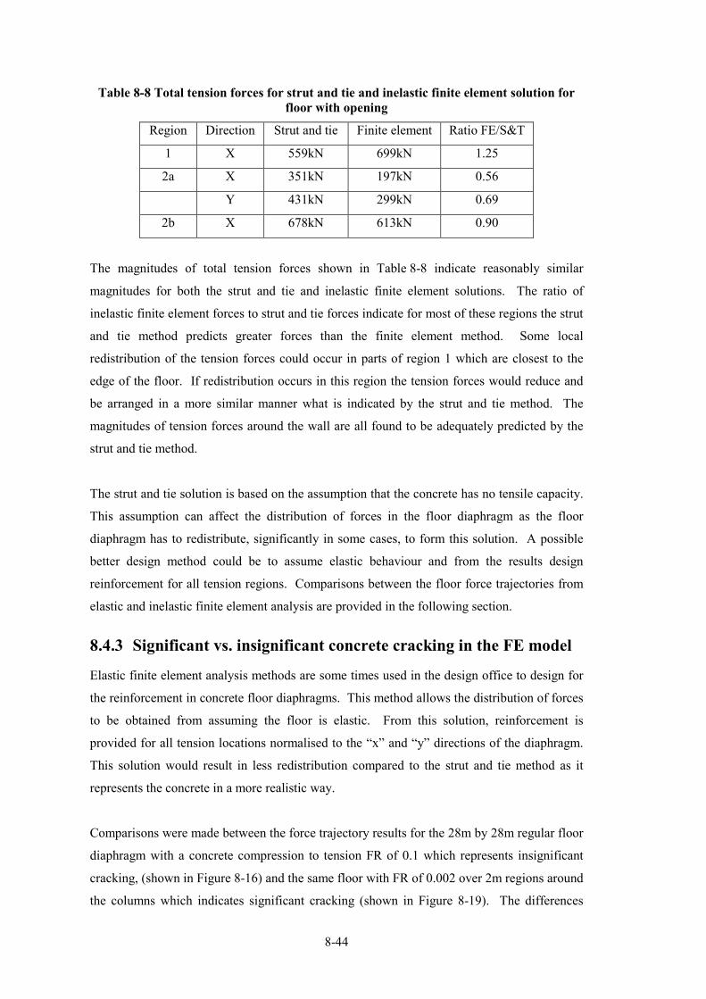
8�44


floor with opening


1 X 559kN 699kN 1.25

2a X 351kN 197kN 0.56

Y 431kN 299kN 0.69

2b X 678kN 613kN 0.90

The magnitudes of total tension forces shown in Table 8�8 indicate reasonably similar

magnitudes for both the strut and tie and inelastic finite element solutions. The ratio of

inelastic finite element forces to strut and tie forces indicate for most of these regions the strut

and tie method predicts greater forces than the finite element method. Some local

redistribution of the tension forces could occur in parts of region 1 which are closest to the

edge of the floor. If redistribution occurs in this region the tension forces would reduce and

be arranged in a more similar manner what is indicated by the strut and tie method. The

magnitudes of tension forces around the wall are all found to be adequately predicted by the

strut and tie method.

The strut and tie solution is based on the assumption that the concrete has no tensile capacity.

This assumption can affect the distribution of forces in the floor diaphragm as the floor

diaphragm has to redistribute, significantly in some cases, to form this solution. A possible

better design method could be to assume elastic behaviour and from the results design

reinforcement for all tension regions. Comparisons between the floor force trajectories from

elastic and inelastic finite element analysis are provided in the following section.

8.4.3 Significant vs. insignificant concrete cracking in the FE model

Elastic finite element analysis methods are some times used in the design office to design for

the reinforcement in concrete floor diaphragms. This method allows the distribution of forces

to be obtained from assuming the floor is elastic. From this solution, reinforcement is

provided for all tension locations normalised to the “x” and “y” directions of the diaphragm.

This solution would result in less redistribution compared to the strut and tie method as it

represents the concrete in a more realistic way.

Comparisons were made between the force trajectory results for the 28m by 28m regular floor

diaphragm with a concrete compression to tension FR of 0.1 which represents insignificant

cracking, (shown in Figure 8�16) and the same floor with FR of 0.002 over 2m regions around

the columns which indicates significant cracking (shown in Figure 8�19). The differences

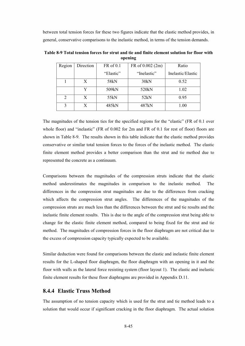
8�45

between total tension forces for these two figures indicate that the elastic method provides, in

general, conservative comparisons to the inelastic method, in terms of the tension demands.

Table 8+9 Total tension forces for strut and tie and finite element solution for floor with

opening

Region Direction FR of 0.1

“Elastic”

FR of 0.002 (2m)

“Inelastic”

Ratio

Inelastic/Elastic

1 X 58kN 30kN 0.52

Y 509kN 520kN 1.02

2 X 55kN 52kN 0.95

3 X 485kN 487kN 1.00

The magnitudes of the tension ties for the specified regions for the “elastic” (FR of 0.1 over

whole floor) and “inelastic” (FR of 0.002 for 2m and FR of 0.1 for rest of floor) floors are

shown in Table 8�9. The results shown in this table indicate that the elastic method provides

conservative or similar total tension forces to the forces of the inelastic method. The elastic

finite element method provides a better comparison than the strut and tie method due to

represented the concrete as a continuum.

Comparisons between the magnitudes of the compression struts indicate that the elastic

method underestimates the magnitudes in comparison to the inelastic method. The

differences in the compression strut magnitudes are due to the differences from cracking

which affects the compression strut angles. The differences of the magnitudes of the

compression struts are much less than the differences between the strut and tie results and the

inelastic finite element results. This is due to the angle of the compression strut being able to

change for the elastic finite element method, compared to being fixed for the strut and tie

method. The magnitudes of compression forces in the floor diaphragm are not critical due to

the excess of compression capacity typically expected to be available.

Similar deduction were found for comparisons between the elastic and inelastic finite element

results for the L�shaped floor diaphragm, the floor diaphragm with an opening in it and the

floor with walls as the lateral force resisting system (floor layout 1). The elastic and inelastic

finite element results for these floor diaphragms are provided in Appendix D.11.

8.4.4 Elastic Truss Method

The assumption of no tension capacity which is used for the strut and tie method leads to a

solution that would occur if significant cracking in the floor diaphragm. The actual solution

8�46

which develops is somewhere between an elastic responding floor diaphragm and a

significantly cracked floor diaphragm. A truss solution was developed for the L�shaped floor

diaphragm which allows both positive and negative tensions in the diagonal struts. This

solution was developed to capture the results for an elastic L�shaped floor.

46KN 92KN

28KN 26KN 38KN 15KN

17KN

3KN38KN

30KN 2KN 8KN

104KN 127KN

264K

N11

2KN

142K

N22

KN

17K

N47

KN

46K

N61

KN

4 3K

N13

KN

39K

N52

KN

19K

N85

KN

99K

N

37K

N

124KN

108KN

104KN

79KN42KN

47KN

21KN

81KN

102KN

34KN

0KN 32KN

79KN123KN

10K

N30

KN

242K

N84

KN

47KN

109K

N

134KN

196KN 157KN

91KN 80KN 42KN 36KN

2KN

76KN104KN

7KN 3KN 5KN

251KN226KN

162K

N55

KN

16K

N72

KN

58K

N27

KN

9KN

50K

N

67K

N6K

N1K

N64

KN

191K

N15

KN

28K

N22

4KN

18KN

1KN

22KN

74KN

41K

N

107KN

72KN

85KN

131K

N

72KN

40KN 34KN

98KN272KN

15K

N13

KN

222K

N25

KN

16KN

96K

N137

KN

142KN

152KN186KN

39KN 25KN 59KN 81KN

20KN

41KN9KN

13KN 18KN 26KN

23KN

57K

N86

KN

85K

N25

8KN

32K

N18

KN

20K

N15

KN

81K

N44

KN

34K

N53

KN

20K

N3

9KN

97KN

82KN

96KN

13KN51KN

78KN

64KN

73KN

66KN

40KN

44KN

79KN

72KN 109KN

166KN

94K

N75

KN

35KN

61KN

13KN

27KN

87KN214KN204KN106KN

47KN

43KN

49KN

369KN

185KN

185KN

369KN 340KN

170KN

340KN356KN

178KN

355KN

185KN

Region 1

Region 3

Region 2

Region 4

21KN

33KN

61KN

76KN

34KN

33KN60KN

18KN148KN

21KN

64KN

39K

N

4KN

63KN

11KN

55KN

15KN

7KN142KN

34KN

67KN

85KN81KN

92KN

110KN

136KN

134KN

89KN

23KN

13KN

49KN

3KN

5KN

29KN

68KN

123K

N

133K

N

114K

N

68KN

77KN

50KN

51KN

29KN

22KN

22KN

22KN

30KN

11KN

4KN

69KN

2KN


KEY:EQ X

Y

Figure 8+29 Truss method force trajectories for L+shape floor with a refined mesh

(3.5m by 3.5m)

Figure 8�29 shows the distribution of forces for a truss solution of the L�shape floor loaded

monotonically in the y�direction (as indicated in the key). The magnitudes of the total tension

forces in the specified regions of the figure are provided in Table 8�10.

8�47

Table 8+10 Total tension forces for truss method and inelastic finite element solution (FR

of 0.002 for 2m around columns) for L+shaped floor

Region Direction Truss Finite element Ratio FE/Truss

1 X 148kN 174kN 1.18

2 X 304kN 478kN 1.57

3 X 270kN 214kN 0.79

Y 142kN 145kN 1.02

4 X 94kN 41kN 0.44

Y 352kN 335kN 0.95

Table 8�10 indicates that the truss method approximates the inelastic finite element (FR of

0.002 for 2m) forces adequately for region 3 and 4. Comparisons between the results from

the Truss method, shown in Table 8�10, and the Strut and Tie method (no tension in the

concrete), shown in Table 8�5, indicates the Strut and Tie method predicts more similar

tension forces to the forces obtained from the inelastic finite element analysis for the tension

tie regions (Region 1 and Region 2) of the floor diaphragm compared to the Truss method.

The Truss method is found to predict more similar forces to the forces from inelastic finite

element analysis at the stress concentration region of the floor (Region 3) compared to the

Strut and Tie method.

8�48

39KN 9KN

24KN 23KN 29KN 3KN

28KN

26KN53KN

32KN 10KN 1KN

114KN 161KN

336K

N14

4KN

179K

N15

KN

21K

N47

KN

9KN

17K

N

63K

N28

KN

36K

N10

4KN

28K

N11

KN

13K

N6K

N

168KN

148KN

140KN

108KN51KN

87KN

27KN

95KN

67KN 95KN

199KN184KN

41K

N1K

N

79K

N1K

N

37KN

201KN 173KN

89KN 63KN 31KN 56KN

38KN

3KN9KN

18KN 10KN 2KN

54KN 25KN

34K

N9K

N9K

N90

KN

7KN

34K

N8K

N45

KN

8 KN

5 KN

20K

N6 7

KN

57K

N25

KN

144K

N34

4KN

65K

N

63KN

77KN

48KN

77KN

103K

N

67KN

3KN 21KN

5KN9KN

2 9K

N3 2

KN

9 KN

1 68K

N

91KN

82KN

85KN

118KN

131KN 161KN


18KN

6KN22KN

65KN 59KN 40KN

23KN

31K

N18

2KN

172K

N38

4KN

16K

N50

KN

66K

N13

KN

54K

N47

KN

81K

N39

KN

2 4K

N4 2

KN

147KN

110KN

89KN

54KN34KN

132KN

92KN

126KN

82KN

27KN

33KN

76KN

69KN

181KN


57KN

36KN

48KN

29KN

5KN 15KN 6KN 15KN

36KN

81KN101KN

34KN 16KN 8KN

204KN 200KN

47K

N12

KN

13K

N16

KN

73K

N8K

N7K

N24

KN

27K

N16

KN

155K

N26

KN

112K

N

102KN

114K

N

159K

N

39KN 57KN

126KN176KN

26K

N58

KN

343K

N13

9KN

87KN

160K

N

172K

N

88KN47K

N

77KN

34KN

28KN

75KN

473KN

236KN

236KN

236KN

472KN

241KN

241KN

241KN

482KN

483KN

55KN

12KN

Region 1

Region 2a

Region 2b

Region 3

6KN10KN

43KN34KN

73KN

45KN

64KN

44KN

55KN

30KN

53KN

85KN

80KN

95KN

74KN

92KN

105KN

50KN

8KN

62KN49KN

79KN

109KN

85KN

73KN

93KN96KN

78KN22K

N

16KN

77KN

99KN124K

N

115KN

95KN52KN

36KN

47KN

98KN155KN

156KN

170KN

8KN12KN

324KN

6KN

26KN

79KN

13KN

0KN

13KN

14KN

152KN

144KN

31KN

49KN

7KN

101K

N

182KN

144K

N14

0KN

115K

N

103KN

135KN

23KN

32KN

10KN

9KN

19KN


KEY:EQ X

Y

Figure 8+30 Truss method force trajectories for floor with an opening and refined mesh

(3.5m by 3.5m)

Figure 8�30 shows the distribution of forces for a truss solution for the floor with a 7m

opening monotonically loaded in the y�direction (as indicated by the key). The magnitudes of

the total tension forces in the specified regions of the figure are provided in Table 8�11.

8�49

Table 8+11 Total tension forces for truss method and inelastic finite element solution (FR

of 0.002 for 2m around columns) for floor with opening

Region Direction Truss Finite element Ratio FE/Truss

1 X 466kN 426kN 0.91

2a X 104kN 165kN 1.59

Y 199kN 216kN 1.09

2b X 141kN 206kN 1.46

Y 156kN 267kN 1.71

3 X 107kN 30kN 0.28

Y 491kN 445kN 0.91

The total tension forces for the truss method and the inelastic finite element method, shown in

Table 8�11, indicate that the truss method under�estimates the values from the inelastic finite

element method (FR of 0.002 for 2m around columns) indicating some zones of

redistribution. Comparisons between these results and the results for the strut and tie method

indicate that the truss method would result in less redistribution for some regions of the floor.

8.4.5 Angles of Forces in the Concrete

The angles of the compression struts and tension ties, which develop within floor diaphragms,

vary due to a number of different factors. The angles of the force trajectories for the 28m by

28m structure are provided in the following figures to help to identify the trends of how the

angles vary. The angles shown in the following figures are the magnitude of the angles from

the x�direction axis, which is given in the key for each figure.

8�50

76

o

67 o

54 o

63 o

48 o

54 o

49 o

47 o

45 o

44 o

44 o

41 o

46 o

45 o

45 o

47 o

46 o45 o

45 o

46 o

48 o

53 o

64 o

55 o

48 o

43 o

44 o

45 o

39 o

36 o

43 o

42 o

38 o

45 o

25 o

37 o

25 o

38 o

28 o

24 o

32 o

25 o

12 o67

o

12o

25o

28o

24o

32o

36o

25o

39o

38o

37o

25o

45o

38o

42o

43o

45o

43o

48o

55o

46o

46o

41o

45o

45o

47o

48o

53o

68o

63o

67o

54o

49o

46o

45o

45o

44o

44o

45o

47o

48o

54o

67

o

76

o

44o

1o

2o

3o

7o

20o

45o

50o

20o

7o

3o

2o

1o

45o

50o

68o

68o

0o

0o

90o

90o

90o

90o

90o

90o

90o

90o

74

o

59 o

58 o

62 o

55 o

60 o

55 o

51 o

45 o

53 o

46 o

40 o

36 o

39 o

42 o

49 o

49 o46 o

36 o

30 o

55 o

59 o

64 o

43 o

60 o

56 o

51 o

49 o

41 o

40 o

47 o

52 o

55 o

45 o

34 o

55 o

41 o

50 o

42 o

44 o

34 o

30 o

16 o

64

o

15o

32o

31o

28o

32o

25o

36o

40o

34o

29o

36o

46o

31o

33o

39o

39o

35o

31o

55o

52o

63o

70o

47o

44o

41o

34o

34o

52o

57o

70o

40o

38o

40o

43o

54o

62o

46o

41o

39o

40o

45o

51

o

63

o

38o

1o

12o

23o

23o

24o

12o

17o

52o

16o

9o

3o

1o

82o

78o

9o

78o

0o

90o

90o

90o

90o

90o

90o

90o

90o


KEY:EQ X

Y

Figure 8+31 Angles of the inelastic finite

element force trajectories for floor with

FR of 0.1



FR of 0.002

Figure 8�31 and Figure 8�32 show the angles of the force trajectories from the inelastic finite

element analysis which developed in the floor diaphragm for the regular floor diaphragm of

28m by 28m. The force trajectory results which these angles are related to are shown in

Figure 8�16 and Figure 8�17.

The angles of concrete compression strut and concrete tension tie forces, which developed in

the central region of the floor diaphragm, away from the perimeter columns, are shown in

general to be around 45 degrees. In the region at the centre of the floor the force angles are

observed to tend towards 0 degrees.

8�51

Comparisons were made between the angles of the forces, located away from the perimeter

columns, for floors with different concrete tension�to�compression failure ratios (described in

Section 8.3.5.1). This comparison indicated that the angles of the concrete compression strut

forces were larger for the significantly cracked floor compared to the angles for the un�

cracked floor. As a consequence of this the angles of the concrete tension ties were smaller

for the significantly cracked floor compared to the angles for the un�cracked floor. These

angles change due to cracking of the concrete altering the stiffness of the floor.

The angles of the compression strut and tension tie forces at the interface between the floor

and the perimeter columns vary depending on the column locations within the floor. The

compression strut angles are shown to be reasonably large for the tension tie end of the floor

and smaller for the compression strut region of the floor. The reason these angles change, for

different column locations within the floor, is due to the magnitude of the inertial forces that

were transferred to each of the columns by the compression struts. For the exterior columns

located in top of the figure, much greater inertial forces are transferred by compression struts

compared to the columns located in the bottom region of the figure. The angles of the

compression struts increase with larger compression forces, as a larger angle requires less

tension force to tie the column back into the floor to satisfy equilibrium. The most desirable

solution for the forces within floor diaphragm is the solution which induces minimum strain

energy in the floor (Schlaich et al., 1987). Greater strain energy is associated with

deformations of reinforcing steel compared to the strain energy associated with deformations

of concrete.

8�52

78

o

68 o

59 o

59 o

58 o

49 o

45 o

53 o

50 o

46 o

44 o

42 o

48 o

45 o

45 o

47 o

44 o44 o

45 o

47 o

50 o

53 o

69 o

58 o

47 o

43 o

43 o

45 o

42 o

38 o

43 o

41 o

37 o

60 o

26 o

31 o

28 o

37 o

22 o

26 o

46 o

22 o

14 o

74

o

10o

18o

20o

29o

32o

21o

20o

34o

38o

35o

22o

46o

42o

44o

42o

45o

44o

46o

48o

46o

47o

41o

47o

46o

45o

49o

52o

56o

59o

73o

49o

47o

45o

45o

45o

43o

44o

46o

48o

54o

60o

65

o

66

o

45o

1o

1o

1o

4o

26o

54o

66o

21o

8o

2o

1o

1o

46o

58o

22o

18o

0o

90o

90o

90o

90o

90o

90o

90o

90o

0o

79

o

62 o

62 o

69 o

57 o

55 o

49 o

52 o

46 o

43 o

41 o

41 o

44 o

43 o

44 o

43 o

45 o44 o

44 o

47 o

46 o

51 o

70 o

61 o

48 o

42 o

43 o

46 o

44 o

34 o

45 o

43 o

37 o

59 o

38 o

30 o

28 o

36 o

31 o

36 o

44 o

42 o

27 o

79x o

9o

27o

15o

27o

30o

31o

15o

35o

37o

34o

21o

42o

38o

44o

43o

46o

45o

48o

40o

49o

47o

29o

48o

47o

46o

56o

55o

47o

49o

63o

54o

52o

49o

46o

46o

42o

43o

44o

46o

53o

68o

60

o

65

o

46o

1o

1o

1o

5o

31o

57o

60o

17o

3o

3o

6o

3o

49o

72o

18o

19o

0o

90o

90o

90o

90o

90o

90o

90o

90o

0o


KEY:EQ X

Y



FR of 0.002 1m around the edge with

FR of 0.1 elsewhere



FR of 0.002 2m around the edge with

FR of 0.1 elsewhere

Figure 8�33 and Figure 8�34 show the force trajectory angles that were obtained for the

regular 28m by 28m floor diaphragms with cracked zones of 1m and 2m loaded

monotonically in the y�direction (indicated by the key). The magnitudes of the angles for the

compression strut forces at and away from the columns are found to be similar in both figures.

Comparisons between angles of the tension tie forces for both of these figures indicate

reasonably similar results. Some small variations in the angles are shown. These variations

are similar to the variations described for the floors with limited and significant cracking,

where the angles of the tension tie forces, at the columns, are shown to reduce for the floor

with greater cracking with a corresponding increase in the compression strut angle.

8�53

Comparisons were made between the angles of the forces shown in these figures to the angles

shown in Figure 8�31 and Figure 8�32. These comparisons indicated that the compression

strut angles, at the interface between the floor and the columns, were larger for both of these

floors, with specified zones of cracking, compared to the angles for the floors with cracking

assigned over the entire floor diaphragm. For these floors the zone of cracking are much

more concentrated which could possibly have caused the compression strut angles at the

floor�to�column interface to increase.

Similar trends to these trends for the regular 28m by 28m diaphragm were observed for the L�

shaped floor diaphragm and openings. These trends are provided in Appendix D.12.

The angles of the force trajectories for a floor diaphragm with walls as the lateral force

resisting system, for layout 1, are provided in Figure 8�35 to Figure 8�38. The angles shown

in these figures represent the magnitudes of the angles measured from the compression strut

or tension tie orientation to the x�axis.

Figure 8�35 and Figure 8�36 indicate the orientation of the force trajectories for floor layout

one with concrete tension to compression failure ratios of 0.1 and 0.002 over the whole floor

respectively. Comparison of these angles indicates the concrete compression strut angles, at

the wall interface, were larger for the severely cracked floor compared to the corresponding

values for the un�cracked floor. The angles are larger for the severely cracked floor which

correlates to the philosophy of developing less strain energy within the reinforcement of the

floor as discussed previously. The concentration of steel forces at the walls, for these floors

with walls, is much larger than at the columns in frames. This is why there is a greater affect

on the angles for these wall results compared to the results from frames.

8�54

70 o

57 o

37 o

48 o

33o

33o

29o

9o

12o

13o

12o

4o

54 o

48 o

36 o

43 o

19o

33o

37o

46o

48

o

39o

44 o

39 o

26 o

34 o

42o

46o

47o

49o

48o

40 o

32 o

19 o

24 o

43o

55o

55o

55o

51o

39 o

30 o

12 o

27 o

37o

61o

65o

64o

52 o

47o

49 o

53 o

57 o

34o

37o

37o

31o

35o

39o

48

o

55 o

49 o

20 o

39 o

4o

0o

0o

44o

51o

42o

42o

0o

0o

0o

0o

0o

0o

Xx

o0

o

0o

0o

6o

13o

30o

63o

0o

0o

69 o

55 o

39 o

47 o

37o

34o

27o

9o

13o

15o

13o

19o

57 o

48 o

31 o

42 o

20o

29o

40o

48o

60

o

38o

49 o

42 o

27 o

35 o

37o

41o

47o

50o

43o

47 o

37 o

19 o

25 o

38o

48o

55o

55o

42o

48 o

33 o

14 o

26 o

34o

52o

64o

62o

57 o

45o

52 o

57 o

66 o

24o

33o

33o

31o

34o

48o

53

o

58 o

54 o

37 o

55 o

4o

0o

0o

41o

36o

35o

30o

0o

0o

0o

0o

0o

0o

0o

0o

0o

0o

8o

21o

33o

55o

0o

0o


KEY:EQ X

Y

Figure 8+35 Angles of the force trajectories

from inelastic finite element analysis for

floor diaphragm with walls and a concrete

tension to compression FR of 0.1




tension to compression FR of 0.002

The magnitudes of the concrete tension tie angles at the wall interface are much larger for the

un�cracked floor compared to the cracked floor. This is due to the development of cracking in

the floor altering the stiffness and causing the concrete tension tie angle to reduce.

The angles of the compression and tension forces in the concrete, away from the walls, are

observed to tend towards zero degrees, similar to the frame results. The force orientation

tends towards zero away from the walls as the forces need to tie the walls together and the

most effective way of doing this is by forces with a zero degree angle. This correlates to large

angles in high shear regions (around the walls) and smaller angles in high moment regions

(away from the wall).

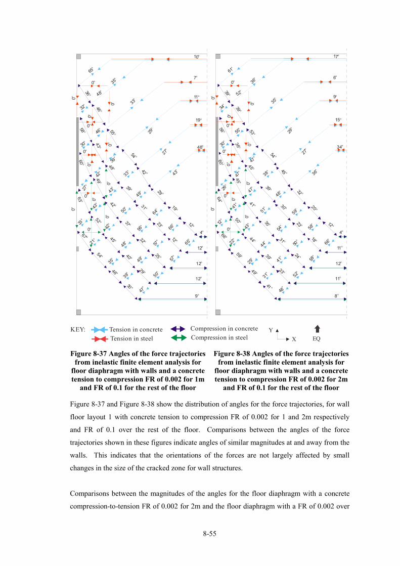
8�55

67 o

54 o

30 o

46 o

35o

33o

33o

9o

12o

12o

12o

10o

52 o

45 o

29 o

40 o

21o

35o

39o

47o

60

o

42o

42 o

37 o

25 o

32 o

43o

48o

49o

50o

50o

39 o

31 o

12 o

23 o

43o

56o

57o

57o

49o

42 o

29 o

12 o

19 o

33o

64o

66o

65o

54 o

65o

48 o

49 o

63 o

27o

42o

39o

29o

27o

43o

43

o

55 o

46 o

36 o

58 o

4o

0o

0o

48o

32o

46o

30o

0o

0o

0o

0o

0o

0o

0o

0o

0o

0o

7o

11o

19o

48o

0o

0o

66 o

59 o

41 o

49 o

36o

35o

12o

8o

11o

12o

11o

17o

50 o

44 o

33 o

39 o

22o

29o

31o

48o

60

o

43o

41 o

35 o

24 o

31 o

41o

44o

41o

52o

51o

39 o

30 o

18 o

23 o

47o

54o

50o

58o

48o

45 o

32 o

12 o

20 o

38o

59o

58o

66o

54 o

61o

45 o

45 o

64 o

26o

47o

47o

29o

27o

36o

36

o

53 o

39 o

39 o

56 o

4o

0o

0o

52o

34o

55o

30o

0o

0o

0o

0o

0o

0o

0o

0o

0o

0o

6o

9o

15o

34o

0o

0o


KEY:EQ X

Y




tension to compression FR of 0.002 for 1m

and FR of 0.1 for the rest of the floor




tension to compression FR of 0.002 for 2m

and FR of 0.1 for the rest of the floor

Figure 8�37 and Figure 8�38 show the distribution of angles for the force trajectories, for wall

floor layout 1 with concrete tension to compression FR of 0.002 for 1 and 2m respectively

and FR of 0.1 over the rest of the floor. Comparisons between the angles of the force

trajectories shown in these figures indicate angles of similar magnitudes at and away from the

walls. This indicates that the orientations of the forces are not largely affected by small

changes in the size of the cracked zone for wall structures.

Comparisons between the magnitudes of the angles for the floor diaphragm with a concrete

compression�to�tension FR of 0.002 for 2m and the floor diaphragm with a FR of 0.002 over

8�56

the entire floor were made. These comparisons indicate that the angles of the forces at the

wall�to�floor interface were similar. Similar forces are expected as cracking has occurred

around the walls for both of these floors. The angles of the compression forces within the

floor diaphragm, away from the walls, are shown to be slightly smaller for the floor

diaphragm with specified cracking regions. This is due to the larger concrete tensile capacity

for this region of the floor. Comparisons between the angles of the concrete tension tie values

within the floor indicate slightly larger angles for the floor with specified cracking regions.

This is due to less cracking of the concrete developing within the floor diaphragm.

Appendix D.12 provide additional results for the angles of the force trajectories which

develop in the floor diaphragm for L�shaped floors, floors with openings and floors with walls

as the lateral force resisting system.

8.4.5.1 Columns

A study was carried out to determine if compression strut angles at columns could be

specified and used in strut and tie methods to improve strut and tie solutions in comparison

with results from inelastic finite element analysis. The affect of the following parameters on

the compression strut angle which develops at the columns were considered in this

investigation:

− Angle of monotonic loading of the floor diaphragm;

− Different concrete tension to compression failure ratios (FRs);

− Different floor diaphragm geometry;

− Relative location of column within the floor diaphragm.

The analytical finite element models used to obtain this data are described in Section 8.3. The

compression strut angle data at the columns which was obtained from the inelastic finite

element analyses is provided in Appendix D13.1.

8�57

Trends of compression strut angles:

θ1

θ2

θ3

θ4

Tfx1

Cf1

Tfx2

Tfx3

Tfx4

Cf2

Cf3

Cf4

Direction of

earthquake

Y

X

Top

Bottom

Figure 8+39 Orientation of compression and tension forces at columns

It was found that the angle between the compression strut and x�direction tension tie, θ, was

much greater in zones where the compression strut into the column was large (Figure 8�39).

The magnitudes of the compression struts differ depending on the loading direction and

location of column around the floor diaphragm. Figure 8�39 indicates the trends of how the

magnitude and angle of compression struts alter within a simple floor diaphragm which is

monotonically loaded in the y�direction. The magnitudes of the compression struts change

from the bottom to the top of the floor due to cracking of the concrete and the interaction from

tension tie forces in the concrete and the beam members. The compression strut angle, with

the x�direction, was found to be smaller at columns where the magnitude of the compression

strut into the columns was small, such as for Cf4, and larger at columns with large

compression strut forces, such as Cf1, as indicated in Figure 8�39.

The data of the different compression strut angles at the columns, provided in

Appendix D.13.1, ranged from an average value of 45 degrees for the columns with small

compression struts to an average of 82 degrees for columns with large compression struts for

all of the floor diaphragm layouts which were described in Section 8.3.1. Negligible

differences between the compression strut angles from the inelastic finite element analysis

with different concrete tension to compression failure ratios (the ratios are provided in Section

8.3.5.1) and with applied forces of different orientations (0 degrees and 45 degrees to the y�

direction) were observed in the data.

8�58

Magnitude of compression struts and tension ties:

The strut and tie method is unable to predict both compression and tension forces which are

greater than the forces predicted by inelastic finite element analysis methods due to the fixed

angles of the compression struts which are used in the strut and tie method. Reinforced

concrete floor diaphragms typically have excess compression capacity and are limited by the

tensile capacity due to the material properties of concrete. Therefore, if a compression strut

angle could be provided for the strut and tie method the angle should be based on an angle

which would lead to tension forces which are greater than the tension forces obtained from

inelastic finite element analysis.

It was determined from the inelastic finite element results (provided in Appendix D13.1) that

the magnitude of the tension tie forces were greatest for the columns in the central region of

the floor (Figure 8�39). This is because for the columns which have large compression strut

forces (at the top of the floor in Figure 8�39) the angle is large therefore the x�component

tension force is small and for the columns with small compression strut forces (at the bottom

of the floor in Figure 8�39) the forces are small and therefore the x�component tension force is

also small.

The average angle between the x�direction and the compression struts at the columns in the

central region of the floor was found to be 65 degrees. If this angle was used to represent the

strut angle for the other columns at the top and bottom of the floor (Figure 8�39), the x�

direction tension ties would be greater than what they were found to be for the inelastic finite

element analysis. The variation of the maximum and minimum actual compression strut

angles from the average value for the columns in the central region of the floor was of the

order of +/� 13 degrees, which is a large variation. An example indicating the affect of this

variation on the magnitudes of tension forces, for the case where the shear removed by the

column is kept constant, is provided in Figure 8�40.

270kN

291kN

126kN

65o

270kN

343kN

211kN

52o

(a) Angle of 65 degrees (b) Angle of 52 degrees

Figure 8+40 Sensitivity of forces with respect to changes in compression strut angle for

columns

This figure shows the effect of changing the compression strut angle on the magnitude of

compression strut and tension tie forces for a constant amount of shear removed by the

8�59

column. This indicates that variations of the angle of the concrete compression struts have a

large affect on the magnitude of both the tension and compression forces which develop at

column node. A smaller angle typically produces larger tension forces and smaller

compression forces if the shear removed by the column remains constant. In terms of the

strut and tie method, it would be prudent to use a smaller compression strut angle due to

tension capacity of a concrete floor diaphragm (between both tensile capacity of the concrete

and that of the reinforcement in the x�direction) typically limiting the strength capacity of the

floor.

From these results strut and tie models with compression strut angles to the columns of

52 degrees (which is �13 degrees from the average value) were developed and consequently

compared to the inelastic finite element analysis results with concrete tension to compression

FR of 0.002 over 2m around the columns. The floors were monotonically loaded in the y�

direction as indicated by the key in the diagrams.

230KN

141KN

177KN

177KN

424KN

95K

N12

7KN

329K

N4

76K

N

100 K

N19

6 KN

201 K

N2

07K

N

242KN

238KN

165KN

236KN

2KN

231KN

291KN

275KN

298KN

169K

N17

7KN

196K

N2

37K

N380KN

473KN

487KN

443KN

230KN

141KN

177KN

177KN

424KN10

0KN

196K

N20

1KN

207K

N

242K

N23

8KN

165K

N

236K

N

291KN

298KN

380K

N47

3KN

487K

N

443K

N

2KN

95K

N12

7KN

329K

N4

76K

N



Y

Figure 8+41 Strut and tie solution for 1:1 geometry floor plan with compression strut

angle of 52 degrees at the columns for coarse mesh

8�60

113KN 66KN 55KN81KN 14KN70KN73KN73KN 102KN84KN 80KN 102KN70KN70KN8KN 109KN

16KN 38KN80KN 69KN30KN61KN137KN74KN 124KN38KN 16KN 134KN64KN35KN75KN 133KN







107KN 107KN110KN 93KN107KN110KN110KN91KN 121KN56KN 68KN 149KN49KN

49KN53KN 110KN

K62N 57KN40KN 46KN 47KN24KN16KN30KN

40KN 34KN25KN 28KN 28KN11KN1KN22KN







112K

N

35KN

35KN

123KN

32KN56KN

59KN

26KN

16KN

32KN

29KN

56KN28KN

35KN15KN

37KN

87K

N80K

N

65KN

95KN

45KN47KN

41KN

20KN

20KN

22KN

17KN

84KN

81K

N93KN

91KN

83KN

71KN61KN

44KN

22KN

17KN

4KN 8K

N

47KN77KN

95KN 118KN

105K

N14KN

3KN

105K

N78KN

96KN

103KN

81KN68KN

42KN

20KN

12KN

KN 40KN

80KN104K

N130KN

102K

N12KN

82K

N85KN

109KN

67KN

86KN66KN

34KN

13KN

6KN

24KN68KN

101KN

144KN

120K

N13KN

87K

N87KN

106KN

55KN

80KN

51KN12KN

4KN

KN 10KN

44KN76KN 133KN

133K

N18KN

122K

N83KN

88KN

61KN

57KN21KN

19K

N

16KN

KN 21KN

29KN81KN

124K

N

27KN

164K

N54KN

57KN

86KN

24KN10KN

31K

N

94KN

8KN

23KN

25KN

51KN 49KN

49KN 9KN 9KN

54KN

61K

N

76K

N

138KN

168K

N

82KN

126KN 31KN

8KN

111K

N

89KN

54KN

73KN 13KN

71KN

95K

N

69K

N

72KN

61KN

61KN 21KN

71KN

75K

N

59K

N

50KN

47KN

80KN

4KN24KN

58KN

55K

N

81K

N

58KN

49KN

45KN 10KN 25KN

60KN

64K

N

49K

N

51KN

49KN

35KN 12KN 22KN

59KN

60K

N

45K

N

33KN48KN

38KN53KN

25K

N

27K

N

14K

N

26K

N

65KN66KN

43KN39KN

87KN70KN

65KN

46KN

13K

N

9KN

13K

N

13K

N

12KN

4KN

3KN

8KN

3KN

98K

N

Region 1

Region 3Region 2

Region 4



Y

Figure 8+42 Strut and tie solution for L+shaped floor with 52 degree compression struts

at columns for refined mesh

Both Figure 8�41 and Figure 8�42 show strut and tie solutions with compression strut angles

of 52 degrees over the regions of the floor where the columns were located for the 28m by

28m floor diaphragm and the L+shaped floor diaphragm, respectively. The corresponding

results from inelastic finite element analysis (FR of 0.002 for 2m around the columns) are

shown in Figure 8�19 and Figure 8�22, respectively and the corresponding results from strut

and tie analysis with 45 degree compression strut angles over the entire floor are shown in

Figure 8�20 and Figure 8�23, respectively. The magnitudes of the total tension forces for the

regions which are specified in the figures are provided in Table 8�12 and Table 8�13.

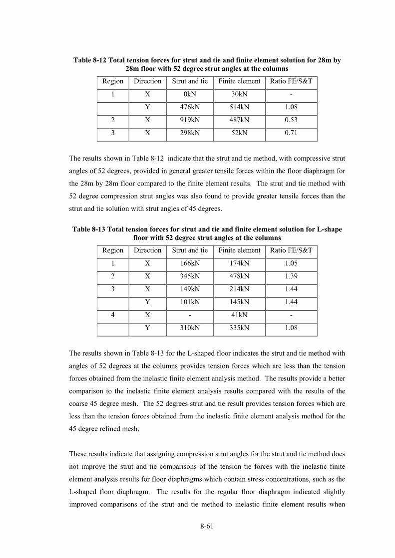
8�61

Table 8+12 Total tension forces for strut and tie and finite element solution for 28m by

28m floor with 52 degree strut angles at the columns


1 X 0kN 30kN �

Y 476kN 514kN 1.08

2 X 919kN 487kN 0.53

3 X 298kN 52kN 0.71

The results shown in Table 8�12 indicate that the strut and tie method, with compressive strut

angles of 52 degrees, provided in general greater tensile forces within the floor diaphragm for

the 28m by 28m floor compared to the finite element results. The strut and tie method with

52 degree compression strut angles was also found to provide greater tensile forces than the

strut and tie solution with strut angles of 45 degrees.

Table 8+13 Total tension forces for strut and tie and finite element solution for L+shape

floor with 52 degree strut angles at the columns


1 X 166kN 174kN 1.05

2 X 345kN 478kN 1.39

3 X 149kN 214kN 1.44

Y 101kN 145kN 1.44

4 X � 41kN �

Y 310kN 335kN 1.08

The results shown in Table 8�13 for the L�shaped floor indicates the strut and tie method with

angles of 52 degrees at the columns provides tension forces which are less than the tension

forces obtained from the inelastic finite element analysis method. The results provide a better

comparison to the inelastic finite element analysis results compared with the results of the

coarse 45 degree mesh. The 52 degrees strut and tie result provides tension forces which are

less than the tension forces obtained from the inelastic finite element analysis method for the

45 degree refined mesh.

These results indicate that assigning compression strut angles for the strut and tie method does

not improve the strut and tie comparisons of the tension tie forces with the inelastic finite

element analysis results for floor diaphragms which contain stress concentrations, such as the

L�shaped floor diaphragm. The results for the regular floor diaphragm indicated slightly

improved comparisons of the strut and tie method to inelastic finite element results when

8�62

compression strut angles were assigned. The additional work and the lack of benefit gain

from assigning compression strut angles in the strut and tie method suggests that compression

strut angles of 45 degrees provide a reasonable approximation to the forces which develop

within floor diaphragms.

8.4.5.2 Walls

The angles of the compression struts at walls for floor diaphragms with wall lateral force

resisting systems were recorded to determine if a compression strut angle could be specified

for the strut and tie method to improve results obtained from the strut and tie method

compared with results from inelastic finite element analyses. The affect of the following

parameters on the compression strut angle which develops at the walls were considered in this

investigation:

− Angle of monotonic loading of the floor diaphragm;

− Different concrete tension to compression FRs;

− Relative location of walls within the floor diaphragm.

The analytical finite element models used to obtain the compression strut angles are described

in Section 8.3. The data used to determine the compression strut angles is provided in

Appendix D.13.2. A number of finite elements exist along the length of the walls resulting in

a range of magnitudes and angles of compression struts. The average of the compression strut

angles along the length of the wall was used for this study. Comment is provided in

Section 8.4.7 regarding how the magnitudes of the compression struts and tension tie forces

varies along the length of the wall.

From the inelastic finite element analysis results it was observed that the average angle

between the compression strut forces and the x�axis, at the floor�to�wall interface, was found

to be around 50 degrees for relatively elastic responding floors (floors with concrete tension

to compression FR of 0.1) and around 60 degrees for floors which were exposed to significant

cracking (floors with FR of 0.002). Section 8.4.5 provides an explanation to why these angles

vary for different levels of cracking within the floor. The maximum and minimum angle sizes

for the struts at the floor�to�wall interface were found to vary respectively by +/� 8 degrees

and +/� 6 degrees for the relatively un�cracked and significantly cracked floor diaphragms

loaded in different directions. The magnitude of forces, in terms of compression struts and

tension ties, to create equilibrium are reasonably sensitive to the compression strut angle, an

example of the sensitivity for 8 and 6 degree angle variations are provided below. For these

cases the magnitude of shear forces resisted by the wall remained constant.

8�63

50o2

611kN

1678kN

200

0kN

2989

kN

2221kN

200

0kN

42o

Compression in concrete Tension in steelKEY:X

Y

EQ

(a) Angle of 50 degrees (b) Angle of 42 degrees


an elastically responding floor (FR of 0.01)

2309

kN

1155kN

200

0kN

2472k

N

1453kN

200

0kN

60o

54o

Compression in concrete Tension in steelKEY:X

Y

EQ

(c) Angle of 60 degrees (d) Angle of 54 degrees


an in+elastically responding floor (FR of 0.002 for 2m around columns)

Figure 8�43 and Figure 8�44 provide a comparison between the magnitudes of compression

and tension forces for variations in the compression strut angle at the floor�to�wall interface

for different levels of inelasticity within the floor. The magnitude of shear forces resisted by

the wall was kept the same for this comparison to indicate the affects of varying the

compression strut angle. These figures clearly show the tension and compression forces are

sensitive to changes in the angles of compression struts. The variation of the compression

strut angles shown in these figures correlates to the maximum variations from the average

angle found in the results. For the elastically responding floor, the magnitude of the

compression strut force was found to vary by 14% for the change in angle and the tension tie

force was found to vary by 32%. For the in�elastically responding floor the magnitude of the

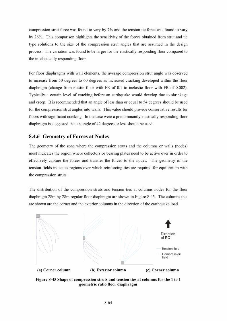
8�64

compression strut force was found to vary by 7% and the tension tie force was found to vary

by 26%. This comparison highlights the sensitivity of the forces obtained from strut and tie

type solutions to the size of the compression strut angles that are assumed in the design

process. The variation was found to be larger for the elastically responding floor compared to

the in�elastically responding floor.

For floor diaphragms with wall elements, the average compression strut angle was observed

to increase from 50 degrees to 60 degrees as increased cracking developed within the floor

diaphragm (change from elastic floor with FR of 0.1 to inelastic floor with FR of 0.002).

Typically a certain level of cracking before an earthquake would develop due to shrinkage

and creep. It is recommended that an angle of less than or equal to 54 degrees should be used

for the compression strut angles into walls. This value should provide conservative results for

floors with significant cracking. In the case were a predominantly elastically responding floor

diaphragm is suggested that an angle of 42 degrees or less should be used.

8.4.6 Geometry of Forces at Nodes

The geometry of the zone where the compression struts and the columns or walls (nodes)

meet indicates the region where collectors or bearing plates need to be active over in order to

effectively capture the forces and transfer the forces to the nodes. The geometry of the

tension fields indicates regions over which reinforcing ties are required for equilibrium with

the compression struts.

The distribution of the compression struts and tension ties at columns nodes for the floor

diaphragm 28m by 28m regular floor diaphragm are shown in Figure 8�45. The columns that

are shown are the corner and the exterior columns in the direction of the earthquake load.

Tension field

Compression field

Direction of EQ

(a) Corner column (b) Exterior column (c) Corner column

Figure 8+45 Shape of compression struts and tension ties at columns for the 1 to 1

geometric ratio floor diaphragm

8�65

Figure 8�45 indicates the geometric distribution of the compression struts (dark blue) and

tension ties (light blue) at the interface of the columns in the floor diaphragm. The

distribution of the compression forces that were observed to enter the corner column (shown

in (a)) are similar to a bottle shaped compression field distribution.

The bottle shaped compression field (Schlaich, J., K. Schafer, et al. (1987)) developed for the

corner columns maximise the amount of inertial forces that can be transferred to the column.

The inertial forces that are not transfer to the corner column in the compression need to be

pulled back across the floor by tension forces to the column node. Therefore by developing a

bottle shaped compression field a more optimal force path solution is developed by

minimizing the strain energy which develops in the floor diaphragm.

The distributions of the compression and tension fields that enter/exit the exterior column

(shown in Figure 8�45(b)) are shown to be slightly different to the distribution of the stress

fields at the corner columns. The general distribution is like a prism stress field distribution

(Schlaich, J., K. Schafer, et al. (1987)) at a distance away from the column and the

distribution close to the column is like a local bottle stress field distribution. The stress

distribution away from the exterior columns is more like a prism due to the surrounding

compression fields that are located around this compression field.

The geometries of the compression and tension fields, which were observed to develop at the

re�entrant corner, for the L�shape floor diaphragm are shown in Figure 8�46.

Figure 8+46 Compression and tension stress fields at the re+entrant corner of the L+

shaped floor

The shape of the compression field shown for the re�entrant corner of the L�shaped structure

is prismatic away from the column and converges locally at the column. This type of strut

would require some kind of collector, in the direction perpendicular to the earthquake, to

Tension field

Compression field

Direction of

EQ Re-entrant

corner Floor

diaphragm

8�66

capture the compression field at the top end of the column. For the results shown in

Figure 8�22 the collector would need to extend around 2m either side of the column,

additional reinforcement may be required for this.

The tension stress field away from the column is of a fanned shaped. The tension stress field

very close to the column is perpendicular to the direction of the earthquake. Consequently, in

the region close to the column, cracking is likely to develop perpendicular to the tension field,

in the same direction to the earthquake. If significant cracking develops in this region,

particularly under cyclic loading, the compression field may not be able to transfer force into

the column. This would consequently require the force paths in this region to redistribute.

The geometries of the forces at the nodes for the floor diaphragms with openings were found

to be similar to the above reported trends. Therefore the geometries of the nodes are not

shown in this section with floor with openings.

Tension field

Compression field

Direction of EQ

Figure 8+47 Compression and tension field at the 7m wall for floor layout 1

The shape of the compression field for the 7m wall is a bottle shape type where the forces

converge at the floor�to�wall interface. This compression field indicates that large

compression forces are present at the end of the wall. Therefore, careful detailing should be

considered around the ends of the walls.

The shape of the tension field for the 7m wall is more of a prism shape. A reason as to why a

prism shaped stress field has developed, rather than a bottle shaped field for the tension field,

could be due to the limited space left in the upper region of the floor diaphragm to transfer the

tension forces. The magnitudes of tension forces which developed at the floor�to�wall

interface were of the order of around 100kN over a 1m length of floor�to�wall interface.

Additional tension steel would be required to resist this tension force.

8�67

Tension field

Compression field

Direction of EQ

Figure 8+48 Compression and tension field at the 7m wall for floor layout 4

The distributions of compression and tension fields shown in Figure 8�48 are similar to the

distributions shown for the 7m walls in floor layout 1 shown in Figure 8�47. The difference is

that the compression field is of the same distribution to the tension field (in the opposite

direction) and likewise for the tension field. As the distributions are similar in terms of the

relative space above/below the walls in the floor diaphragm it is concluded that the shape of

the stress field is affected when the space for the stress field to develop is limited.

Tension field

Compression field

Direction

of EQ

Figure 8+49 Compression and tension stress field distribution for floor layout 3

The distributions of both the tension and compression stress fields shown in Figure 8�49 are

similar to the distributions shown above for the floors with different orientations of walls.

The tension forces for the 14m wall are also affected by the location of the wall at the edge of

the floor diaphragm.

8.4.7 Distribution of Forces at Walls

The distribution of the concrete compression and tension forces that act on the walls were

found to be irregularly distributed. This is different to the distribution that is assumed in

8�68

practice. In practice, it is assumed that the forces enter the wall from the floor with evenly

distributed magnitudes along the length of the wall, and therefore a uniform distribution of

steel is supplied in the design.

0

20

40

60

80

100

120

140

14 15 16 17 18 19 20 21

Fo

rce

(k

N)

Distance along the wall

Distribution of total tension forces along the length of the wall for floor layout 1

Figure 8+50 Distribution of total tension forces along the length of the wall for floor

layout 1

Figure 8�50 shows the distribution of the tension forces over the length of the wall (the wall

length spans between 14m to 21m in layout 1). This figure indicates that the distribution of

forces over the length of the wall is not uniform and that the magnitudes of the forces are

larger at the ends of the wall. This variation in the distribution of forces needs to be

considered to ensure the magnitude of the peak force is not significantly larger than the

average force and therefore would not result in significant cracking developing at the floor�to�

wall interface. This situation could lead to undesirable performance of some of the brittle

precast flooring systems that are used in New Zealand construction.

Table 8+14 Ratio of peak force+to+average force for floor layouts

Floor layout Floor layout Wall Ratio

1 7�14�7 A 1.2

2 14�14�14 A 1.1

3 7�28�7 A 1.3

4 7�28�7 A 1.3

The magnitudes of the total tension forces from the floors were examined in this section to

assess how the maximum tension forces compared to the average tension forces. The ratios

between these tension force values, for each of the wall floor layouts, are shown in

Table 8�14. The floor layout numbers provided in this table correlate to the wall layouts

8�69

provided in Table 8�2. These ratios refer to the maximum�to�average ratio of the x�direction

total tension force over the length of the wall.

These results indicated that the maximum tension forces ranged between 1.1 to 1.3 times

larger than the average tension forces. No trends could be identified with regards to the ratio

of maximum to average tension forces for different floor diaphragm wall layouts. Additional

floors with in different locations were investigated to determine the affects of the relative

position of the walls on the maximum�to�average tension force ratio. The floor layouts

included in this study and the maximum�to�average tension force ratios obtained from this

study are shown in Table 8�15.

Table 8+15 Trends of the ratio of peak force to average force

Floor layout Wall A Wall B Wall C Wall Ratio

Irregular wall layout:

7�14�7 y:14�21m x:14�21m y:21�28m A 1.2

B 1.2

7�14�7 y:14�21m x:14�21m y:7�14m A 1.2

B 1.5

14�14�14 y:7�21m x:14�21m y:14�28m A 1.1

B 1.1

Variation of walls location:

7�14�7 y:7�14m x:14�21m y:7�14 A 1.4

7�14�7 y:21�28m x:14�21m y:21�28 A 1.2

7�28�7 y:21�28m x:7�28m y:21�28 A 1.1

14�14�14 y:7�21m x:14�21m y:7�21m A 1.2

The results, shown in Table 8�15, indicate that the largest variation of the maximum�to�

average force ratio is related to the position of the walls. As the y�direction walls get closer to

the x�axis (y=0), the force ratio increases. The ratio increases because the region which needs

to be tied together, beyond the walls, is much greater when the y�direction walls are close to

y=0 on the x�axis. Therefore a concentration of tension forces develops at the end of the wall

which is the greatest distance from the x�axis, as the end of the wall is trying to tie the rest of

the floor together.

The comparisons between the tension forces from the Strut and Tie method and the inelastic

finite element analysis method (FR of 0.002 for 2m), in Section 8.4.2, indicated that the Strut

and Tie method predicted larger tension forces. Comparisons of the total tension forces that

8�70

were predicted by the Strut and Tie method, along the length of walls, to the forces from the

inelastic finite element method were made to determine how to deal with the concentrations

of forces that have been found to develop along the length of walls in this Section. The

results from these comparisons are shown in Table 8�16. The S&T to FE category, shown in

this table, represents the ratio of the average strut and tie forces at the wall interface to the

maximum recorded steel tension force from the inelastic finite element method (FR of 0.002

for 2m around the columns). Floor layout 5* refers to the irregular wall layout 7�14�7 with

walls located at y:14�21m, x:14�21m and y:7�14m; the results shown are for wall y:7�14m.

This wall layout was included as it was shown to produce the largest peak force to average

force ratio in Table 8�15.

Table 8+16 Ratio of average strut and tie force to max force

Floor layout Floor layout Wall S&T/FE

1 7�14�7 A 1.31

2 14�14�14 A 2.35

3 7�28�7 A 1.29

4 7�28�7 A 1.30

5* 7�14�7 B 1.24

The results shown in this table indicate that the average strut and tie forces are greater than

the maximum tension in the steel recorded from inelastic finite element analysis. These

results indicate that the large tension forces which can develop over the length of the wall

would be accounted for by the conservatism associated with the Strut and tie Method for

regular floor diaphragms with walls as the lateral force resisting system. Therefore additional

factors to represent the maximum tension forces are not necessary as they would result in

overly conservative results when Strut and Tie methods are used.

8.5 Conclusions

Trends associated with internal forces which develop in floor diaphragms have been

investigated in this chapter. A variety of floor diaphragm geometries have been included

which represent typically constructed structural systems. The key findings from this study are

summarised in the following paragraphs.

Reviews of past experimental floor diaphragm testing indicated that significant cracking

formed in the floor diaphragm around the perimeter columns over a distance of 1 to 2m.

Comparisons were made between the total tension forces for floors with different zones of

assigned cracking. This included an elastic floor, a fully cracked floor and floors with 1m and

8�71

2m cracked zones around the perimeter columns and elastic for the remaining regions. These

comparisons indicated:

− The forces which develop in floor diaphragms are sensitive to the level of concrete

tension capacity assumed;

− Variations of the size of the cracking region of 1�2m did not have a large affect on the

results.

Comparisons were made between the distributions of in�plane floor diaphragm forces for two

different analytical modelling elements; finite elements and lattice elements. The finite

elements represent the continuum of the reinforced concrete floor diaphragm whereas, the

lattice element represents the floor by discrete truss members (horizontal, vertical and

diagonal to represent the shear and axial behaviour) assumed to represent an equivalent

stiffness of the floor diaphragm. Comparisons of the distributions of floor diaphragm forces,

for these two analytical modelling elements, indicated differences. The distributions differed

due to the discrete trusses, and the fixed angle of the shear struts used in the lattice element.

It is therefore recommended, that discrete methods, such as the lattice element method, should

not be employed for analyses where the distributions of forces in a continuous material is

important to the outcome of the analyses.

Comparisons were made between the total tension forces from the elastic and inelastic finite

element analysis solutions and the strut and tie solutions. The findings from these

comparisons indicated:

− The total tension forces were adequately predicted by the strut and tie method for a

regular floor diaphragm for most regions. The strut and tie method could not predict

accurately the local tension forces which developed around one of the corner

columns;

− The total tension forces for the strut and tie solution for the L�shaped floor diaphragm

provided a poor prediction of the total tension forces when compared to the values

from inelastic finite element analysis. Refinement of the strut and tie solution (from

7m by 7m to 3.5m by 3.5m) was carried out which lead to better predictions of the

total tension forces with comparison to inelastic finite element analysis results;

− For a floor diaphragm with an opening the coarse strut and tie method was found to

provide a poor prediction of total tension forces compared with the inelastic finite

element results, especially around the opening. A refined strut and tie solution was

developed (from 7m by 7m to 3.5m by 3.5m) but comparisons with the finite element

results were again poor;

8�72

− The strut and tie solution provided a conservative approximation to the finite element

solution for floor diaphragms with walls.

These results indicate that significant redistributions could occur. To minimise redistributions

it is advised to continue to refine the mesh of nodes for the strut and tie solutions until no

changes occur. The regions which large redistributions could develop include: around the re�

entrant corner, the opening and corner columns.

Comparisons were made between the results from elastic and inelastic finite element methods.

These results indicated that the elastic finite element method provided predominantly good

comparisons in terms of the tension forces to the inelastic finite element results. The elastic

finite element method provides better comparisons, compared to the strut and tie method, as

more realistic strut angles are used. The elastic finite element method also represents the

solution before cracking occurs in the concrete and therefore results in a solution with less

redistribution.

From these comparisons it is recommended that in the case where a floor diaphragm has

potential stress concentration regions and redistribution cracking is undesirable elastic finite

element analysis should be employed. For floor diaphragms which are not expected to have

significant stress concentrations the strut and tie method may be used.

The angles of the compression struts were investigated in this study. It was found for a

perimeter frame structure the angle of the compression struts at the floor�to�columns interface

varied depending on the location of the column within the structure. The angles of the forces

in the floor diaphragm were found to change due to increased cracking causing changes of the

stiffness and also due to minimising the strain energy within the floor. The average of the

angles the compression struts (measured in the direction perpendicular to the wall) were

found to be:

− 65 degrees with +/� 13 degrees variation for the columns;

− 50 degrees for no concrete cracking in the floor diaphragm with +/�8 degrees

variation for the walls;

− 60 degrees for significant concrete cracking in floor for walls.

Strut and tie solution were developed using these angle sizes. Comparisons between the strut

and tie results with these angles and the inelastic finite element results indicated that using

these angles did not significantly improve the comparisons to the finite element results.

8�73

The distribution of the total tension forces which developed along the length of the walls were

found to vary and not be uniform as is assumed in practice. Investigations of the maximum

forces were made to ensure undesirable performance of some of the brittle precast flooring

systems that are used in New Zealand construction would not occur. Comparison of the

maximum forces from the inelastic finite element method with the forces from strut and tie

methods indicated that the maximum forces were less than the forces predicted by the strut

and tie method for walls. Therefore additional allowance for these forces was not required as

it is accounted for in the conservatism of the strut and tie method for wall structures.

8.6 References

ABAQUS (2004a). ABAQUS/CAE Version 6.7�1, ABAQUS, Inc.

ABAQUS (2004b). ABAQUS Analysis user manual version 6.7 online documentation.

Ang, B. G. (1985). Seismic Shear Strength of Circular Bridge Piers. Departement of Civil

Engineering. Christchurch, University of Canterbury. Doctor of Philosophy.

Blandón, J. J. and M. E. Rodriguez (2005). "Behavior of Connections and Floor Diaphrgms in

Seismic�Resisting Precast Concrete Buildings." PCI Journal 50(2): 56�75.



Engineering 37(2).



Canterbury.

Hrennikoff, A. (1941). "Solution of Problems of Elasticity by the Framework Method."

Journal of Applied Mechanics 8(4): 169�175.

Jensen, J. (2004). Diaphragm Action Issues in a Jointed Precast Concrete System. Final year

project report, Department of Civil Engineering, University of Canterbury, NZ.

Kolston, D. and B. W. Buchanan (1980). "Diaphragms in Seismic Resistant Buildings."

Bulletin of the New Zealand Soicety for Earthquake Engineering 12(2): 162�170.

Lee, Y. and K. J. Willam (1997). "Anisotropic Vertix Plasticity Formulation for Concrete In�

Plane Stress." Journal of Engineering Mechanics 123(7): 714�726.

8�74






Philosophy.

Mau, S. T. and T. Hsu, T. C;, (1987). "Shear Behaviour of Reinforced Concrete Framed Wall

Panels with Vertical loads." ACI Structural Journal 84(3): 228�234.

NZCS (1994). Revisions to the New Zealand Standard for the Design of Concrete

Structures:NZS3101. Technical report No. 15 (TR15). N. Z. C. Society.

Paulay, T. and M. J. N. Priestley (1992). Seismic Design of Reinforced Concrete and


Research Engineers Ltd (1999). STAAD/Pro QSE Plan Frame. Almondsbury, Bristol, UK.,

Draycott House.

Schlaich, J., K. Schafer, et al. (1987). "Toward a Consistent Design of Structural Concrete "

PCI Journal 32(3): 74�149.


New Zealand.



Vecchio, F. J. and M. P. Collins (1986). "The Modified Compression�Field Theory for

Reinforced Concrete Elements Subjected to Shear." ACI Journal 83(2): 219�231.

9�1

9 CONCLUSIONS

9.1 Summary

The trends and magnitudes of seismic forces which develop in floors of multi�storey buildings

were investigated in this research project. Two types of forces develop in floor diaphragms,

namely: inertial and self strain forces. Inertial floor forces develop due to the accelerations of

the mass of the floor diaphragm. There are a number of types of self strain forces, these

include: forces which develop in structures with lateral force resisting elements of different

deformation patterns (referred to as “transfer forces”), forces induced due to elongation of

plastic hinges and forces due to p�delta affects. All of these forces, except self strain forces

due to elongation of plastic hinge, were considered in this study. Details of the key findings

from this research are provided in Section 9.2. Limitations of these findings and suggestions

for extensions to this research are provided in Section 9.3. An overview of the research that

was carried out is presented in the following paragraphs.

The trends associated with compatibility self strain transfer forces which develop in floor

diaphragms were investigated. A preliminary study using pushover analyses was carried out

to determine fundamental trends. Non�linear time history analyses were carried out to ensure

that the interaction between inertial and transfer forces could be captured in the results. The

following variations were included in the time history analysis study to determine further

trends:

− Variations of the stiffness ratio for frame�to�wall (dual) structures;

− Variations of the structural ductility factors of dual structures;

− Variations of the flexibilities of dual structures;

− Variations of the strength of the floor diaphragm in dual structures;

− Variations of the stiffness of the floor diaphragm in dual structures;

− Variations of the heights of dual structures;

− Variation of seismicity level including low and high seismicity regions;

− Type of lateral force resisting system including: walls and podium structures.

The sensitivities of modelling assumptions on the magnitudes of floor diaphragm forces were

investigated using non�linear time history analyses. The modelling assumptions that were

investigated included the affects of: foundation flexibility, shear deformation and variations in

9�2

the beam, column and wall plastic hinge model used to represent stiffness degradation of the

materials.

The trends of inertial forces for moment resisting frame structures were also investigated by

non�linear time history analyses. A range of buildings were developed including: different

heights, soil conditions and different levels of seismicity.

An analytical model, which was developed by Peng (2009) to predict the plastic hinge zones

of beams, was modified to enable the performance of structural walls to be predicted by time

history analysis. The predictions obtained using the modified model were found to compare

satisfactory with load deformation results obtained from seven experimental wall tests from

the literature.

A simplified floor diaphragm design method, which gives a set of static floor forces, was

developed with the intension of use in the design office. Satisfactory comparisons of transfer

and inertia forces were obtained between results from non�linear time history analyses and

results from this floor design method. These comparisons indicated that this design method

provides an adequate approach for the design of floor diaphragms. Three dimensional time

history analyses were also carried out to validate that the design method is appropriate for

design of torsionally susceptible buildings.

An investigation was carried out on the distribution of inertial floor forces for a range of

different floor diaphragms including:

− Perimeter frame floor;

− L�shaped floor;

− Floors with openings;

− Floors with walls at the lateral force resisting elements.

Finite element and strut and tie methods were used to determine the distribution of diaphragm

forces. The finite element model represented cracking of concrete and indicated both the

tension and compression forces which developed in both the concrete and reinforcement of

the floor. The outputs from the finite element method were considered to provide the most

accurate estimate of the floor diaphragm forces. Comparisons were made between the total

tension force, which developed in the concrete and reinforcement in specific regions of the

floor, to indicate the amount of cracking due to redistribution of forces within the floor.

9�3

9.2 Key Findings

The main findings obtained from this research are detailed in the following sections.

9.2.1 Transfer Forces

The influence of the variations of parameters described in Section 9.1 on the magnitudes of

transfer forces were identified from the pushover and time history analyses that are described

in Chapter 2. Two dimensional frame�to�wall dual structures were used for these analyses.

The trends determined from these analyses included:

− The magnitudes of transfer forces were found to be largest for the first few dynamic

modes of the structure. This is because the displacements, which induce transfer

forces, are largest for these modes;

− The magnitudes of transfer forces in floor diaphragms were observed to be less for

structures with large frame�to�wall stiffness ratios. This is because the flexible

element provides very little resistance to the deformations imposed by the stiff

element;

− Large transfer forces with the floors, acting as diaphragms, have been found to

develop in structures where the relative stiffness of the vertical elements such as

frame and wall elements are of similar magnitudes and the structure is of a reasonable

height (greater than 3�stories). This occurs as both elements are stiff enough to resist

the actual deformation pattern of the other element (if deforming in isolation).

− The magnitudes of the transfer forces were found to change direction (sign) in the

floor diaphragm (represented by a spring member in the models) compared to inertial

forces for the upper level of the frame�to�wall structures. This is due to the different

deformation patterns for these elements; at the lower levels of the building the wall is

typically stiffer than the frame and at the upper levels the frame has deflected less

than the upper levels of the walls.

− Inelastic deformation of a structure results in permanent lateral deformations, which

induces residual forces in the floors.

− Inelastic action in the diaphragm between the wall and the frame element is found to

reduce the residual transfer forces but may not completely remove these.

− Elastic analysis of the various buildings has been found to poorly predict transfer

force results and is not recommended for any type of analysis where transfer forces

maybe significant. Also elastic analysis of these structures does not identify the

development of residual transfer forces in the structure.

− The magnitudes of transfer forces were found to be insignificant for flexible

structures which are typically built in low seismic regions, such as Auckland;

9�4

− Large transfer forces were found to occur in the floors of podium structures, as

expected. These large transfer forces occurred at the interface of the podium and the

tower. Transfer forces were found to be less when the podium of the structure was

located higher relative to the tower.

− Transfer forces were found to develop in the floor diaphragms of structures with

walls of different length. These forces predominantly formed in the lower floor levels

where the deformation patterns of the walls differed;

− It was found that if inertia and transfer forces were treated separately, poor

predictions were obtained for the total force in the upper and lower levels of the

structure and reasonable comparisons were found for the middle levels of the

structure. This indicates firstly, that inertia and transfer forces are coupled and should

not be treated as separate load cases, to be combined at a later stage of design and

secondly, that maximum inertia and transfer forces occur at similar times in the

middle levels of the structure but not at the upper and lower levels;

9.2.2 Modelling of Structures with Transfer Forces

A sensitivity study, described in Chapter 3, was carried out to determine the affect of different

modelling simplifications on the magnitudes of transfer forces within floor diaphragms.

Modelling simplifications such as the: foundation model, shear deformation and beam column

and wall plastic hinge behaviour were investigated. The foundation models considered

included: a rigid foundation, a simple foundation which lumped the foundation flexibility at

one point and a foundation model which considered the distributed flexibility of both the soil

and piles. The affects of shear deformation on floor forces were considered by including and

excluding the affects of shear deformation on the wall elements. The affects of the plastic

hinge model was examined by creating similar buildings with either a lumped plastic hinge

model or a distributed plastic hinge model. The change in stiffness for the lumped plastic

hinge model was located at one point whereas the change in stiffness for the distributed hinge

model was gradual, as indicated by Figure 9�1.

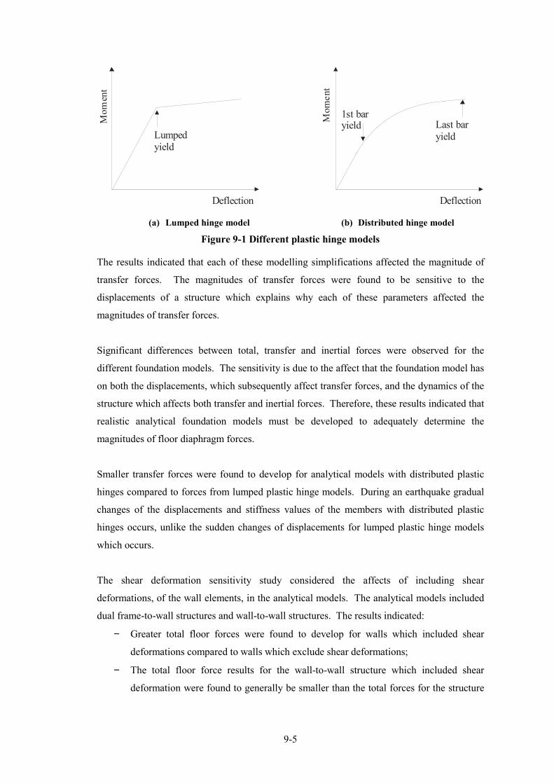
9�5

DeflectionDeflection

Mom

ent

Mo

men

t

1st bar yield Last bar

yieldLumped yield

(a) Lumped hinge model (b) Distributed hinge model

Figure 9(1 Different plastic hinge models

The results indicated that each of these modelling simplifications affected the magnitude of

transfer forces. The magnitudes of transfer forces were found to be sensitive to the

displacements of a structure which explains why each of these parameters affected the

magnitudes of transfer forces.

Significant differences between total, transfer and inertial forces were observed for the

different foundation models. The sensitivity is due to the affect that the foundation model has

on both the displacements, which subsequently affect transfer forces, and the dynamics of the

structure which affects both transfer and inertial forces. Therefore, these results indicated that

realistic analytical foundation models must be developed to adequately determine the

magnitudes of floor diaphragm forces.

Smaller transfer forces were found to develop for analytical models with distributed plastic

hinges compared to forces from lumped plastic hinge models. During an earthquake gradual

changes of the displacements and stiffness values of the members with distributed plastic

hinges occurs, unlike the sudden changes of displacements for lumped plastic hinge models

which occurs.

The shear deformation sensitivity study considered the affects of including shear

deformations, of the wall elements, in the analytical models. The analytical models included

dual frame�to�wall structures and wall�to�wall structures. The results indicated:

− Greater total floor forces were found to develop for walls which included shear

deformations compared to walls which exclude shear deformations;

− The total floor force results for the wall�to�wall structure which included shear

deformation were found to generally be smaller than the total forces for the structure

9�6

which excluded shear deformations; this was not the case for wall�to�wall structures

with stiffness ratios greater than 1:24.

It is recommended that both foundation compliance and wall shear deformation, for frame�to�

wall structures of all stiffness ratios and wall�to�wall structures with stiffness ratios of greater

than 1:24, should be included in analytical models developed to determine the magnitudes of

total floor diaphragm forces. Neglecting these modelling parameters has been shown to lead

to total force results that are less than the forces if the modelling parameters were included in

the inelastic time history analysis.

The comparisons between total forces for different plastic hinge models, “lumped” and

“distributed”, indicated that a “lumped” plastic hinge model leads to total force results which

were larger than the “distributed” plastic hinge model. Therefore, a more sophisticated

distributed plastic hinge model is not required for modelling these types of structures.

Transfer forces, rather than inertial forces, were predominantly affected by the different types

of plastic hinge model. This is because the distributed inelastic behaviour of a plastic hinge

can reduce the displacement incompatibilities between lateral force resisting elements.


Studies were carried out in Chapter 2 and 3 on the magnitudes of inertial forces in the floor

diaphragms for wall�frame (dual) structures and moment resisting frame structures. These

studies indicated:

− That the inertial forces which developed in the floors were affected by high dynamic

modes of the structure;

− Large inertial forces were found in the floors of lower levels of the structure. These

forces where found to be greater than the forces predicted by the Equivalent Static

Analysis (ESA) method described in Section 5.5.

9.2.4 pseudo(Equivalent Static Analysis Design Method

The pseudo�Equivalent Static Analysis (pESA) design method is described in Chapter 5. This

method was developed as a simple desktop design method for estimating the magnitude of

total floor diaphragm forces. This method uses available software to carryout static and

pushover analysis required by this method. The inertial force values obtained from this static

method were compared to the average of the peak inertial forces values, which corresponded

to the maximum combination of transfer and inertial forces, obtained from inelastic time

history analysis. These comparisons indicated that the pESA method adequately predicted the

inertial forces obtained from the inelastic time history results.

9�7

Comparisons were made between the displacements obtained from these two methods to

indirectly compare the magnitudes of transfer forces. The displacements were used as the

displacements control the magnitudes of transfer forces. It was found that the displacements

predicted by the pESA method were less than the displacements predicted by inelastic time

history analysis. A displacement modification method was subsequently developed. The

comparisons between the modified pESA displacements and the time history displacements

indicated that the pESA method predicted displacements which were larger than the

displacements obtained from inelastic time history analysis. A summary of how to carry out

the pESA method was presented in Section 5.6.

Limitations associated with the use of this floor force design method (pESA) are listed in the

following:

− The analytical structures included in this study had elastic fundamental periods

between 0.3s to 1.8s for dual structures and 0.3 to 2.7s for moment resisting frame

structures. The parameters of the model were calibrated for structures with

fundamental periods in this range and therefore this method should not be used for

structures with elastic fundamental periods which lie out of this range;

− The method has been satisfactorily compared with non�linear time history analyses

results for soil types A, B C and D. These soil types are defined in the New Zealand

Design Actions Standard were included (Standards New Zealand, 2004a);

− The floor diaphragms of dual structures with frame�to�wall stiffness ratios up to

SR1:2.6 are allowed to be designed using this method. This correlates to a stiffness

eccentricity of 0.2b where b is the width of the floor diaphragm perpendicular to the

earthquake direction;

− Transfer forces were obtained from structures designed for beam sway mechanisms,

column side sway mechanisms were not considered in this study.

9.2.5 Wall Model

An analytical wall model was developed in this research; this model is described in Chapter 6.

This model accounted for spread reinforcement typical in wall members. Comparisons were

made between analytical and experimental force�displacement and shear�distortion plots

obtained from 7 wall tests reported in the literature. Adequate post yield results were

obtained for the majority of the comparisons between the analytical and experimental

responses for the walls.

The limitations of the use of this wall element include:

9�8

− The yield strength of longitudinal bars to the yield strength of transverse

reinforcement ratios and axial load factors were used to determine the shear flexibility

factors (Section 6.3.4) and contact stress parameters (Section 6.3.6) in the analytical

model. The limits for the yield strength of longitudinal bars to the yield strength of

transverse reinforcement ratio were between 0.44 and 1.79 and the limits for the axial

load factors (Section 6.4) were 0.002 to 0.092;

− This model is not to be used to represent the behaviour of walls with large axial loads

such as coupled walls. Only a limited number of comparisons were made between

the analytical results and experimental results for walls with external loads that were

greater than gravity loads;

− This analytical model should only be used for walls with longitudinal and transverse

reinforcement layouts. The steel filament springs which represent the reinforcement

in this model represent these layouts;

− The analytical model was found for some of the comparisons in Section 6.4 to

provided poor representations of the experimental results for small displacements.

This model should only be used for walls which are exposed to displacements which

are greater than the expected yield displacement of the wall where consideration is

given to the cracked stiffness values;

− The analytical wall model was found to poorly predict the unloading stiffness for a

small number of the comparisons as indicated in Section 6.4. Poor predictions of the

unloading stiffness could affect the response of other members when exposed to small

forces. This analytical model should therefore only be used where the maximum

responses are of interest.

9.2.6 Strut and Tie Method

Comparisons were made between the total tension forces (tension forces in the concrete and

steel) over similar regions from the inelastic finite element analysis solutions and strut and tie

solutions. The findings from these comparisons indicated:

− The total tension forces were adequately predicted by the strut and tie method for a

regular floor diaphragm for most regions. The strut and tie method could not predict

the local tension forces which developed around the corner columns;

− The total tension forces determined by a strut and tie solution for the L�shaped floor

diaphragm, over regions of the floor diaphragm close to columns or stress

concentrations, provided a poor prediction of the total tension forces obtained over an

equivalent region from the finite element analyses. Refinement of the strut and tie

solution (from 7m by 7m to 3.5m by 3.5m) was carried out and a solution within 30%

9�9

of the forces indicated by the inelastic finite element method was obtained indicating

insignificant redistribution cracking would occur;

− Comparisons between the coarse mesh (7m by 7m) strut and tie solution and the finite

element solution, for a floor diaphragm with an opening, indicated significant

redistribution cracking would develop, especially around the opening. A refined strut

and tie solution was (3.5m by 3.5m) compared with the finite element results; the

tension forces predicted by the strut and tie method were found to be less than the

tension forces obtained by inelastic finite element analysis indicating redistribution

cracking would develop;

− For floor diaphragms with walls, the strut and tie solution provided larger tension

forces with comparison to the tension forces obtained by the inelastic finite element

solution indicating insignificant zones of cracking would develop;

− The strut and tie method for all floors, predicted compression forces which were less

than the compression forces predicted by the inelastic finite element method. The

maximum compression forces indicated by the finite element analysis were found to

be less than the permissible maximum crushing strength of the concrete (Standards

New Zealand, 2006) in the floor diaphragm.

These results indicate that significant redistributions of internal forces, associated with

localised extensive cracking of the concrete of the floor diaphragms, could occur for some

floor diaphragms designed by the strut and tie method. To minimise redistributions, it is

advised to refine strut and tie solutions until insignificant changes in the forces are obtained.

The regions which large redistributions could develop include around: re�entrant corners,

openings and corner columns.

Comparisons were made between the results from elastic and inelastic finite element methods.

These results indicated that the elastic finite element method provided predominantly larger

total tension forces in comparisons with the forces predicted by the inelastic finite element

analysis. This method provides better comparisons, compared to the strut and tie method, as

more realistic force trajectories developed due to the continuous nature of the solution. This

method also represents the solution before cracking occurs in the concrete and therefore

results in a solution with less redistribution compared to the strut and tie method, which

represents a fully cracked solution. Limitations on using elastic finite element analysis

include: the knowledge and time it takes to set up a model in comparison to as strut and tie

solution, the limited availability of finite element analysis software in design offices and the

costs of finite element analysis software.

9�10

The results from an elastic truss method, where it was assumed the diagonal members could

sustain both tension and compression forces, were obtained and compared. The tension

forces in the diagonals and the horizontal or vertical members were added to give the total

tension forces for different regions of the floor. This method represented the elastic case.

Comparisons of this method to inelastic finite element results, for both the L�shaped floor and

floor with an opening, indicated that this method provided tension forces which were greater

than the tension forces provided by the inelastic finite element analysis method for some

regions that the strut and tie method predicted forces which were less than the tension forces

predicted by the inelastic finite element method. Connections between the floor and the

columns and walls in a structure are important; it is desirable to minimise the amount of

redistribution which develops around these regions to avoid loss of load paths. Therefore to

minimise the redistribution, it is suggested that both the strut and tie method and the elastic

truss method are used in conjunction and reinforcement is provided for the largest tension

forces from both methods, for the different regions in the floor diaphragm.

The results from this study indicated, when the strut and tie mesh was refined to a point where

the magnitudes of tension forces in the floor diaphragm where not significantly changing, the

tension forces obtained from the strut and tie method were less than the tension forces

obtained from the inelastic finite element analysis method by a percentage of around 30%.

Differences in the tension forces of this magnitude are believed to result in acceptable levels

of cracking redistribution within the floor diaphragm. From this, it is concluded that the strut

and tie method is an acceptable method to model the force trajectories which develop in floor

diaphragms and it is also acceptable to design the amount of reinforcement required within

the floor diaphragm.

9.2.7 Trends of In(plane Floor Diaphragm Forces

Reviews of past experimental floor diaphragm testing indicated that zones of significant

cracking of between 1 to 2m developed around the perimeter columns of floor diaphragms. A

sensitivity analysis was carried out, described in Chapter 8, to determine how the magnitudes

of in�plan forces were affect by different cracked regions. It was found that the distribution of

forces in floor diaphragms are affected by the level of cracking, but for small variations of the

cracking region size, of 1 to 2m around columns, insignificant variations of the forces were

observed.

The angles of the compression struts were investigated in this study. It was found for a

perimeter frame structure the angle of the compression struts at the floor�to�columns interface

9�11

varied depending on the location of the column within the structure. The angles of the forces

in the floor diaphragm were found to change due to increased cracking in the floor causing

changes of the stiffness and subsequently minimising the strain energy within the floor. The

average size of the compressions strut angles (measured in the direction perpendicular to the

wall or frame) were found to be:

− 65 degrees with +/� 13 degrees variation for the columns;

− 50 degrees for no concrete cracking in the floor diaphragm with +/�8 degrees

variation for the walls;

− 60 degrees for significant concrete cracking in floor for walls.

Strut and tie solution were developed using these angle sizes. Comparisons between the strut

and tie results with these angles and the inelastic finite element results indicated that using

these angles did not improve the comparisons to the finite element results.

The magnitude of tension forces, which developed along the length of the walls were found to

vary in Section 8.4.7. This is different to practice where the distribution of tension forces is

assumed to be uniform. Investigations of the maximum tension forces were made to ensure

undesirable performance of some of the brittle precast flooring systems that are used in

New Zealand construction would not occur. Comparison of the maximum tension forces

obtained from inelastic finite element analysis, which developed along the length of the walls,

with the forces from strut and tie methods indicated that the maximum of the tension forces

along the length of the wall were less than the tension forces predicted by the strut and tie

method for walls. The results indicated that the strut and tie method typically predicted

tension forces which were greater than 25% larger than the maximum tension forces at the

floor to wall interface obtained by the inelastic finite element analysis method. Therefore

additional allowance for these forces when using the strut and tie method is not required for

all cases investigated in Section 8.4.7 as the maximum tension forces are accounted for in the

conservatism of the strut and tie method for wall structures.

9.3 Suggested Future Research

Extension could be made to some of the studies that were carried out in this research. These

extensions are listed below. Elaborations to some of these suggestions for future research are

provided in the following paragraphs.

− Further comparisons could be made between the pESA method and time history

analysis for:

o Soil type E;

9�12

o Torsionally restrained and unrestrained structures (as defined in Chapter 7) to

better define the use of the pESA method for torsionally susceptible

structures;

− Determine whether there is a size of openings within floor diaphragms which has an

insignificant affect on the magnitudes and distributions of floor forces and therefore

could be safely ignored in design;

− Consideration of the distribution of transfer forces within the floor diaphragm for

three dimensional dual structures (or for other structural systems);

− Investigation on the magnitudes of forces at the connections between the floor,

columns and walls, to determine whether current detailing practices of the

connections are adequate;

− Consideration of the affects of elongation of plastic hinge zones in beams on transfer

forces of the floor and columns of the structural system;

− Investigate how delamination between precast flooring units and the topping slab may

affect the distribution of forces which develop in floor diaphragms;

− Investigate the affects of localised damage zones in the floor diaphragm on the force

paths when force paths are lost due to elongation affects;

− Investigation of how different longitudinal reinforcement ratios in beams, subjected

to beam elongation, affect the damage between the floor diaphragm and the adjacent

beam. Determine when failure “mode 1” and “mode 2” occurs, which is shown in

Figure 9�2 and described in Matthews (2004).

Additional sensitivity studies on torsionally susceptible structures, with varying structural

parameters (strength, stiffness and mass eccentricities) is recommended to further investigate

the ability of the pESA method to predict floor diaphragm forces for these types of structures.

The design and detailing of floor diaphragms could be improved by indentifying the size of

openings that have insignificant affects on floor forces, and therefore could be ignored in the

design process. To determine the affects of openings, considerations should be given to the:

size and location of the opening within the floor, reinforcing within the floor, shape of the

floor diaphragm and location of adjacent lateral force resisting elements.

Determination of the distribution of transfer forces across floor diaphragms would contribute

to the understanding of the locations within a floor diaphragm where stress concentrations

may develop. To successfully do this, an analytical model which could realistically represent

the following would be required:

9�13

− The deformations of the structural system to capture correct transfer forces, including

an appropriate foundation and wall shear deformation models, as determined in

Chapter 3;

− Model the inelastic material behaviour of the floor diaphragm and the inelastic

response of the connections between the floor and the vertical lateral force resisting

elements. Reduction of stiffness and strength of the floor diaphragm was found in

Chapter 2 to reduce transfer forces;

− Inelastic finite elements to model the floor to represent realistic orientations of the

floor forces.

Experimental testing of a floor diaphragm super assemblage by Matthews (2004) resulted in a

gap opening between the floor diaphragm and the beam due beam elongation causing the

adjoining column to drift. A consequence of this gap opening was the loss of floor diaprhagm

support and further, the loss of force paths to the columns. Bull (2003) suggested that one of

two types of deformation modes could develop during a major earthquake. These modes are

shown in Figure 9�2.

(a) Mode 1 – beam plastic hinge

rotates to allow for beam

elongation

(b) Mode 2 – Entire beam rotates to

allow for beam elongation

Figure 9(2 Possible deformation modes as a result of beam elongation (Bull, 2003)

The demec readings from the experimental testing were used to determine the gap growth of

the floor diaphragm and also the mode of the beam to floor connection failure that developed

for Matthews experimental study. Figure 9�3 shows the demec readings for the growth

between the floor diaphragm and the east and west beams.

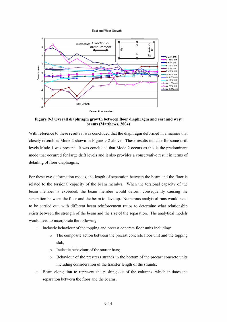
9�14

Figure 9(3 Overall diaphragm growth between floor diaphragm and east and west

beams (Matthews, 2004)

With reference to these results it was concluded that the diaphragm deformed in a manner that

closely resembles Mode 2 shown in Figure 9�2 above. These results indicate for some drift

levels Mode 1 was present. It was concluded that Mode 2 occurs as this is the predominant

mode that occurred for large drift levels and it also provides a conservative result in terms of

detailing of floor diaphragms.

For these two deformation modes, the length of separation between the beam and the floor is

related to the torsional capacity of the beam member. When the torsional capacity of the

beam member is exceeded, the beam member would deform consequently causing the

separation between the floor and the beam to develop. Numerous analytical runs would need

to be carried out, with different beam reinforcement ratios to determine what relationship

exists between the strength of the beam and the size of the separation. The analytical models

would need to incorporate the following:

− Inelastic behaviour of the topping and precast concrete floor units including:

o The composite action between the precast concrete floor unit and the topping

slab;

o Inelastic behaviour of the starter bars;

o Behaviour of the prestress strands in the bottom of the precast concrete units

including consideration of the transfer length of the strands;

− Beam elongation to represent the pushing out of the columns, which initiates the

separation between the floor and the beams;

9�15

− Realistic models of the connection between adjacent precast concrete units with

considerations for the affects of stones lodging in the gap between the support

structure (beams and walls) and the ends of the precast units;

− Realistic representation of the connections between the precast concrete floor units

and the beam which incorporate realistic friction;

− Consideration of the contact behaviour between the beam and the adjacent precast

concrete unit where the precast unit is not seated on the beam;

− The shear behaviour between the topping and hollow�core unit. It may be difficult to

model the shear delamination failure mode due to limitations of engineering

methodologies in the current available literature.

Verifications of the analytical model could be made by comparisons with previous

experimental testing carried out by Matthews (2004), Lindsay (2004) and MacPherson

(2005). Models representing the construction techniques used in each of these experimental

tests would be useful in identifying the performance of past construction techniques and also

assist with developing retrofit solutions.

Unless someone like you,

cares a whole awful lot,

nothing is going to get better.

Its not.

Seuss (1971)

9.4 References



Engineering 37(2).




9�16

MacPherson, C. (2005). Seismic Performance and Forensic Analysis of a Precast Concrete

Hollow�Core Floor Super�Assemblage. Department of Civil Engineering.

Christchurch, University of Canterbury. Masters of Engineering.



Philosophy.




Seuss Geisel, T., (Dr Seuss) (1971). The Lorax, Randon House, New York, USA.


New Zealand.



design recommendations and methods

Documents