HAL Id: tel-02149704https://tel.archives-ouvertes.fr/tel-02149704

Submitted on 6 Jun 2019

HAL is a multi-disciplinary open accessarchive for the deposit and dissemination of sci-entific research documents, whether they are pub-lished or not. The documents may come fromteaching and research institutions in France orabroad, or from public or private research centers.

L’archive ouverte pluridisciplinaire HAL, estdestinée au dépôt et à la diffusion de documentsscientifiques de niveau recherche, publiés ou non,émanant des établissements d’enseignement et derecherche français ou étrangers, des laboratoirespublics ou privés.

Design of the Cherenkov TOF whole-body PET scannerusing GATE simulation

Marharyta Alokhina

To cite this version:Marharyta Alokhina. Design of the Cherenkov TOF whole-body PET scanner using GATE simulation.Medical Physics [physics.med-ph]. Université Paris Saclay (COmUE); Kiïvskij nacìonalnij unìversitetimeni Tarasa Ševčenka (Ukraine), 2018. English. NNT : 2018SACLS279. tel-02149704

NNT

:2018SACLS279

Design of the Cherenkov TOFwhole-body PET scanner using

GATE simulationThese de doctorat de l’Universite Paris-Saclay et de Taras Shevchenko National

University of Kyivpreparee a l’Universite Paris-Sud au sein du CEA-Saclay

Ecole doctorale n576 Particules, Hadrons, Energie, Noyau, Instrumentation, Imagerie,Cosmos et Simulation (PHENIICS)

Specialite de doctorat: Imagerie medicale et radioactivite

These presentee et soutenue a Gif-sur-Yvette, le 20 Septembre 2018, par

Marharyta Alokhina

Composition du Jury :

Achille StocchiProfesseur, Universite Paris-Sud, Directeur de Recherche, Laboratoirede l’Accelerateur Lineaire

President

Gerard MontarouDirecteur de Recherche, CNRS, Laboratoire de Physique deClermont-Ferrand

Rapporteur

Klaus Peter SchafersProfesseur, Westfalische Wilhelms-Universitat Munster Rapporteur

Oleg BezshyykoProfesseur, Taras Shevchenko National University of Kyiv Examinateur

Viatcheslav SharyyIngenieur-chercheur, IRFU, CEA Directeur de these

Igor KadenkoProfesseur, Taras Shevchenko National University of Kyiv Co-directeur de these

2

To my parents

3

4

Contents

List of abbreviations and acronyms 7

Introduction 20

1 Positron Emission Tomography 221.1 Main Principle . . . . . . . . . . . . . . . . . . . . . . . . . . . . . . 221.2 Types of PET scanners . . . . . . . . . . . . . . . . . . . . . . . . . . 241.3 Isotopes production . . . . . . . . . . . . . . . . . . . . . . . . . . . . 26

1.3.1 Cyclotron . . . . . . . . . . . . . . . . . . . . . . . . . . . . . 261.3.2 Ion source . . . . . . . . . . . . . . . . . . . . . . . . . . . . . 271.3.3 Positron emitter production . . . . . . . . . . . . . . . . . . . 28

1.4 Physics in PET . . . . . . . . . . . . . . . . . . . . . . . . . . . . . . 291.4.1 Positron decay . . . . . . . . . . . . . . . . . . . . . . . . . . 291.4.2 Interaction of high energy photons with matter . . . . . . . . 32

1.4.2.1 Photoelectric effect . . . . . . . . . . . . . . . . . . . 321.4.2.2 Compton scattering . . . . . . . . . . . . . . . . . . 331.4.2.3 Pair production . . . . . . . . . . . . . . . . . . . . . 351.4.2.4 Attenuation of photons . . . . . . . . . . . . . . . . . 36

1.4.3 Interaction of optical photons with matter . . . . . . . . . . . 381.4.3.1 Rayleigh and Mie scattering . . . . . . . . . . . . . . 391.4.3.2 UNIFIED model . . . . . . . . . . . . . . . . . . . . 39

1.4.4 Charged particle interaction with matter . . . . . . . . . . . . 391.4.4.1 Cherenkov radiation . . . . . . . . . . . . . . . . . . 40

2 Instrumentation in PET 432.1 Main characteristics of the detectors for PET . . . . . . . . . . . . . 43

2.1.1 Sensitivity . . . . . . . . . . . . . . . . . . . . . . . . . . . . . 432.1.2 Energy resolution . . . . . . . . . . . . . . . . . . . . . . . . . 442.1.3 Spatial resolution . . . . . . . . . . . . . . . . . . . . . . . . . 462.1.4 Timing resolution . . . . . . . . . . . . . . . . . . . . . . . . . 47

2.2 Conventional approach: scintillators . . . . . . . . . . . . . . . . . . . 49

5

2.3 Non-conventional approaches . . . . . . . . . . . . . . . . . . . . . . . 502.4 Data Acquisition. Types of coincidences . . . . . . . . . . . . . . . . 502.5 Image reconstruction algorithms in PET . . . . . . . . . . . . . . . . 53

2.5.1 Analytical . . . . . . . . . . . . . . . . . . . . . . . . . . . . . 542.5.2 Iterative . . . . . . . . . . . . . . . . . . . . . . . . . . . . . . 542.5.3 CASToR platform for image reconstruction . . . . . . . . . . . 55

2.6 Corrections . . . . . . . . . . . . . . . . . . . . . . . . . . . . . . . . 562.6.1 Normalization . . . . . . . . . . . . . . . . . . . . . . . . . . . 572.6.2 Attenuation correction . . . . . . . . . . . . . . . . . . . . . . 582.6.3 Scatter correction . . . . . . . . . . . . . . . . . . . . . . . . . 582.6.4 Random correction . . . . . . . . . . . . . . . . . . . . . . . . 58

2.7 Main directions of improvement in PET . . . . . . . . . . . . . . . . 602.7.1 Reconstruction DOI . . . . . . . . . . . . . . . . . . . . . . . 602.7.2 Transition from 2D-PET to 3D-PET imaging . . . . . . . . . 602.7.3 Use of combined modalities: PET/CT, PET/MRI . . . . . . . 612.7.4 TOF PET . . . . . . . . . . . . . . . . . . . . . . . . . . . . . 61

3 Modeling 663.1 GATE simulation software . . . . . . . . . . . . . . . . . . . . . . . . 663.2 Choice of the Cherenkov radiator . . . . . . . . . . . . . . . . . . . . 673.3 Photodetection . . . . . . . . . . . . . . . . . . . . . . . . . . . . . . 69

3.3.1 MCP-PMT . . . . . . . . . . . . . . . . . . . . . . . . . . . . 693.3.2 Optical interfaces . . . . . . . . . . . . . . . . . . . . . . . . . 773.3.3 Crystal coating and detection surfaces . . . . . . . . . . . . . 77

3.4 Simulated scanner geometry . . . . . . . . . . . . . . . . . . . . . . . 82

4 PET performance estimation according to the NEMA NU 2-2007Standard 844.1 CRT . . . . . . . . . . . . . . . . . . . . . . . . . . . . . . . . . . . . 844.2 NECR . . . . . . . . . . . . . . . . . . . . . . . . . . . . . . . . . . . 85

4.2.1 Phantom NEMA for NECR . . . . . . . . . . . . . . . . . . . 864.3 Spatial Resolution . . . . . . . . . . . . . . . . . . . . . . . . . . . . . 914.4 Image quality and Contrast Recovery Coefficients (CRC) . . . . . . . 96

Conclusion 106

Acknowledgements 108

References 109

6

List of abbreviations and acronyms

CRC ... contrast recovery coefficient

CRT ... coincidence resolving time

CT ... computed tomography

DOI ... depth of interaction

DQR ... dark count rate

FOV ... field of view

GATE ... Geant4 Application for Tomographic Emission

IRFU ... Institute of Research into the Fundamental Laws of the Universe

kcps ... kilo counts per second

LOR ... line of response

MCP ... micro-channel-plate

MLEM ... Maximum Likelihood Expectation Maximization

MRI ... Magnetic Resonance Imaging

NEMA ... National Electrical Manufacturers Association

OP-OSEM ... Ordinary Poisson Ordered-Subset Expectation Maximization

PET ... positron emission tomography

PMT ... photo-multiplier tube

ROI ... region of interest

SiPM ... silicon photo-multiplier

SNR ... signal-to-noise ratio

TOF ... time-of-flight

TTS ... transit time spread

7

Resume

Dans cette these, nous presentons la conception et l’etude de performance d’untomographe par emission de positrons (TEP) corps entier utilisant la radiationTcherenkov avec et sans capacite de temps-de-vol. Nous les comparons aux parametrescorrespondants de la machine TEP commerciale Discovery D-690 de General Electrics.Nos resultats sont basees sur des simulations GATE et tiennent en compte des recom-mandations du Standard NEMA NU 2-2007 pour les scanners TEP.

Le logiciel GATE est un logiciel de simulation Monte Carlo developpe par lacollaboration OpenGATE sur la base du logiciel Geant4. Il permet de simuler lesinstallations de tomographie par emission de positrons, la tomographie par trans-mission, la radiotherapie et l’imagerie optique. En particulier, il permet de menerdes etudes complexes commencant par le suivi de chaque particule dans le cristaljusqu’a la prediction finale de reponse du detecteur.

De plus, nous avons calcule nos images TEP a l’aide de l’algorithme de recon-struction MLEM implemente dans le logiciel ”open-source” CASToR developpe parla collaboration francaise. La qualite d’image (plus precisement, les coefficientsde recuperation du contraste) est comparable a la qualite d’image permises par lescanner TEP conventionnel.

Le Chapitre 1 passe en revue la tomographie par emission de positrons en tantque technique de medecine nucleaire. La premier paragraphe est consacre au principefondamental de la tomographie, qui repose sur la desintegration β+ du traceurradioactif. Le positron emis s’annihile avec un electron du tissu. Deux rayonsgamma de 511 keV sont emis ”dos-a-dos” et peuvent etre enregistres en coıncidencepar la paire de detecteurs dedies. Les lignes de reponse (LOR) relient les pointsde detection des deux photons et permettent de reconstruire la distribution detraceur lorsque un nombre de coıncidences suffisant est accumule. Typiquementun examen dure 20 minutes avec un taux de comptage de quelques millions decoıncidences par seconde. Dans le deuxieme paragraphe, les avantages et les limitesde trois configurations de scanners TEP sont examines: les scanners pour petitsanimaux, les scanners cerebraux et les scanners corps entier. A titre d’exemple,les parametres geometriques du scanner commercial corps entier, Discovery D-690de General Electrics, sont presentes. Le troisieme paragraphe decrit la procedurede production d’isotopes pour le TEP, y compris le principe de fonctionnementdu cyclotron, la configuration de la source d’ions et la production d’emetteurs depositrons.

La quatrieme partie du Chapitre 1 est consacree decrit les processus physiquesintervenant dans le TEP, tels que la desintegration des positrons, l’interaction desphotons de haute energie avec la matiere (l’effet photoelectrique et la diffusion Comp-ton et l’attenuation correspondant du nombre de photons, l’interaction des photons

8

optiques avec la matiere. Enfin, le modele UNIFIED de Geant4 est d’ecrit car nousl’utilisons pour simuler la propagation des photons optiques (reflexion, refraction,

absorption). A la fin du Chapitre 1, un cas particulier d’interaction des particuleschargees avec la matiere, le rayonnement de Tcherenkov est decrit en details.

Le Chapitre 2 decrit une revue de l’instrumentation pour la TEP. Le premierparagraphe examine les parametres principaux des detecteurs pour la TEP, telsque la sensibilite, l’energie, les resolutions spatiales et temporelles. Les deuxiemeet troisieme paragraphes decrivent respectivement les approches conventionnelles(basees sur les cristaux scintillants) et non conventionnelles (utilisant d’autres materiauxde detection tels que liquides et gaz). Le quatrieme paragraphe est consacre al’acquisition de donnees et au format de donnees utilisees en TEP. Plus precisement,les definitions de l’evenement unique (single) dans TEP, trois types de coıncidences(true, random et scatter) et, en outre, les regles de selection de coıncidences disponiblesdans GATE sont presentes. Dans la cinquieme partie du Chapitre 2, deux algo-rithmes de reconstruction d’image en TEP, analytique et iteratif, sont discutes.En particulier, le logiciel CASToR qui est utilise pour la reconstruction d’imageimplementes les algorithmes de reconstruction iteratives. Le sixieme paragraphedecrit la normalisation de donnees et trois types de corrections utilises dans la TEP,a savoir, les corrections d’attenuation, de diffusion et les corrections de coıncidencesfortuites. L’application de ces corrections est necessaire pour obtenir une imaged’une bonne qualite. Tout d’abord, les photons d’annihilation situes a differentsendroits du corps du patient ou du fantome traversent differentes epaisseurs ets’attenuent donc differemment selon le chemin. Le scanner TEP typique contientdes milliers de cristaux disposes en blocs et relies a plusieurs centaines de PMT. Enraison des variations du gain des PMT et de la variation des parametres physiquedu detecteur, l’efficacite de detection varie d’une paire de detecteur a l’autre, ce quientraıne une non-uniformite des donnees brutes. Une procedure de normalisation estutilisee pour reduire cet effet. Les coıncidences fortuites sont dues a une coıncidencealeatoire de photons de deux desintegrations differentes. Les coıncidences fortuitescreent un arriere-plan non correles d’une image TEP acquise et diminuent donc lecontraste d’image si aucune correction n’est appliquee aux donnees. La section suiv-ante, discute des quatre axes principaux d’amelioration de l’imagerie TEP: recon-struction de la profondeur d’interaction (DOI), passage de l’imagerie 2D a l’imagerie3D, utilisation des modalites combinees avec TEP, telles que la tomodensitometrie oul’imagerie par resonance magnetique. Le Chapitre 2 se termine par une presentationdu principe de la technique du temps de vol.

Le Chapitre 3 presente les resultats de simulation obtenus dans cette these. Ilcommence par une description du logiciel de simulation GATE. Dans le deuxiemeparagraphe, notre choix du fluorure de plomb cristallin (PbF2) comme radiateurTcherenkov est explique. L’histoire de l’utilisation du PbF2 pour la detection de

9

particule et de ses proprietes y est presentee. L’attention principale est portee surl’analyse des processus internes dans le cristal PbF2. Nous avons analyse les pro-prietes des particules generees sur chaque etape de la production et de leur trans-port dans le cristal. En particulier, nous presentons dans de chapitre la distributiondes nombres d’electrons par photon de 511 keV, le spectre d’energie des electronsgeneres, la distribution des nombres de photons generes par electron, la distributiondes photons generes par electron en cas de photoionisation uniquement (la selectionpar une energie electronique superieure a 423 keV a ete appliquee), le spectre desphotons optiques par longueur d’onde generee dans un cristal de fluorure de plomb.Le principe de photodetection, le mode de fonctionnement et les principales car-acteristiques du photomultiplicateur a micro-canaux (MCP-PMT) sont examinesdans la troisieme partie du Chapitre 3.

Un parametre crucial de la simulation est la description de l’interface optiqueentre le cristal de fluorure de plomb et la surface de la photocathode. Nous avonsexamine deux options possibles pour l’interface optique: 1) le collage (”adherence”)moleculaire est simule comme une absence de tout media entre le cristal PbF2 et lafenetre PMT et la distance entre le cristal et la fenetre est egale a zero; 2) L’usage degel optique OCF452 (densite 2.33 g/cm3, transparent pour les photons de longueurd’onde λ superieure a 300 nm, indice de refraction de 1.572 a 400 nm).

Pour reduire les pertes de photons a l’interface optique dans le cas du collagemoleculaire, nous avons simule la fenetre PMT faite avec le saphir d’epaisseur 1.3 mmcar ce materiau presente un indice de refraction similaire a celui du cristal PbF2.Nous avons egalement inclus dans les simulations l’efficacite quantique d’une pho-tocathode bialcaline et deux options pour l’efficacite d’absorption des photons op-tiques: un cas ideal avec une efficacite quantique de 100 % et realiste, extrait de lafiche technique.

Dans le cas du collage moleculaire, nous avons observe que nous detectons unnombre significatif de photons de longueur d’onde 250 - 300 nm, ce qui n’est paspossible si le gel optique est utilise en raison de son manque de transparence. Lenombre correspondant de photoelectrons generes a la photocathode est presente.Comme le montre le spectre, nous devons definir un seuil de detection inferieur aun photoelectron afin d’obtenir une efficacite de dtection superieure a 30 %. C’estla raison principale pour laquelle, dans ce projet, nous ne pouvons pas d’utiliser lesphotodetecteur SiPM. En effet, ces detecteurs ont un taux de comptage d’obscurite(DQR) extremement eleve, d’environ 100 kHz/mm2, lorsque le seuil de detection estinferieur a un photoelectron. Cela entraıne un grand nombre de coıncidences fortu-ites et rend irraliste l’utilisation de SiPM dans un scanner Tcherenkov, sans reduirele DQR, par exemple, par le nouveau design de SiPM, ou par le refroidissement abasses temperatures.

L’efficacite de collection des photons optiques depend directement du revetement

10

du cristal. Pour etudier l’influence du revetement de cristal sur l’efficacite totale et laresolution temporelle du scanner, nous avons etudie divers types de revetement et detraitement de la surface du cristal. Nous avons presente resultats pour trois types desurface de cristal PbF2: blanc diffus, noir et poli. Le revetement blanc diffus reflechitla lumiere de maniere uniforme et independamment de l’angle d’incidence avec uneprobabilite d’environ 95 %. La surface noire absorbe 100 % de la lumiere incidenteet seul les photons optiques qui vont directement a la photocathode a partir du pointd’interaction peuvent etre enregistres. De ce fait, la dispersion de la longueur desparcours de photons est minimale et la resolution en temps est optimisee, au prixd’un rendement faible, car seul un petit nombre de photons est enregistre. Pour lerevetement poli, les photons suivent la lois de Fresnel de transmission et de reflexionet les surfaces sont peintes en blanc sur la face arriere, avec une probabilite dereflexion de 95 %.

Nous avons estime la resolution en temps (coincidence resolving time or CRT)pour trois types de revetement de cristal avec une source radioactive ponctuelleplacee au centre entre deux cristaux. Nous avons constate que le revetement noirpermet d’atteindre des resolutions en temps ”optiques” extremement elevees, maisles technologies PMT actuelles ne nous permettent pas de l’utiliser pleinement, etle detecteur final sera limite par le temps de transit (TTS) du PMT. En plus, cetteconfiguration a une efficacite presque trois fois plus faible que les deux autres, ce quidegrade les performances du scanner. Nous avons simule une epaisseur de cristaldeux fois plus elevee (20 mm). Nous observons une degradation considerable duCRT, et l’amelioration modeste de l’efficacite de la detection.

Enfin, sur la base de nos resultats avec deux cristaux, nous avons simule lescanner dans une configuration corps entier. Nous avons choisi d’associer un seulcristal PbF2 a chaque anode du MCP-PMT, et donc chaque module de detectionest compose d’un PMT et de 64 cristaux de taille 6.5 × 6.5 × 10 (20) mm3, collesensemble. Nous avons suppose que chaque cristal individuel est optiquement isoledes voisins et sa surface est de type blanc diffus. La configuration avec trois anneauxde detection donne un champ de vue (FOV) axial de 180 mm. Nous avons teste deuxdiam’etres d’anneau de detecteur de 81 cm et 91 cm. Chaque anneau est constituede 43 ou 48 blocs de detection et pour les diametres de 81 cm et 91 cm, le nombretotal de PMT est en consequence de 129 ou 144. Le nombre total de cristaux est de8256 ou 9216. Nous avons constate que le taux de ”noise equivalent count” (NECR)est optimal pour un diametre de 81 cm. Nous avons egalement edie l’option d’unblindage de plomb pour proteger le scanner des photons hors FOV. Nous avonsconstate qu’un blindage en forme d’anneau avec un diametre interieur de 70 cm,un diametre exterieur de 108 cm et une epaisseur de 3 cm reduit la contribution endehors du FOV et ameliore NECR de 20 %.

Le Chapitre 4 conclut les etudes realisees et presente l’estimation de la perfor-

11

mance TEP envisagee, en particulier: calcul de CRT, de NECR, des coefficientsde recouvrement de contraste (CRC) et de la resolution spatiale du scanner simuleconformement au norme NEMA NU 2-2007. Le premier paragraphe decrit le testpour une estimation plus realiste du CRT lorsque l’ecart TTS du temps PMT de80 ps est pris en compte. Nous avons simule un fantome de test en polyethylene,identique a celui utilise pour le calcul du NECR. Comme on pouvait s’y attendre, lesmeilleures performances sont obtenues pour le cristal de 10 mm d’epaisseur montepar adherence moleculaire. Nous avons observe une degradation importante, plusforte que anticipee, dans la configuration avec une epaisseur de cristal de 20 mm. Letroisieme paragraphe est consacre a l’estimation de la resolution spatiale du scan-ner. Nous observons une degradation entre le centre de FOV a une peripherie de4,5 a 6,5 mm, qui est comparable a la resolution spatiale du scanner conventionnelDiscovery D-690. La configuration en collage mol’eculaire a une resolution spa-tiale comparable a celle du gel optique et legerement amelioree lorsque comparee ala resolution spatiale des scanners classiques. Cela s’explique par le fait que dansnotre configuration, la taille du cristal et le champ de vue sont similaires a ceuxdu scanner classique, mais nous utilisons des cristaux de PbF2 de faibles paisseurs,10 mm, et donc l’erreur de parallaxe en raison de l’incertitude sur le DOI est pluspetite. De plus, le cristal PbF2 a une fraction photoelectrique deux fois plus eleveeque les cristaux LYSO et, donc le nombre d’evenements avec deux points de conver-sion (une diffusion Compton puis une photo-ionisation) est plus petit. La resolutionspatiale de tels evenements est se degrade, lorsque ces conversions ont lieu dans lesdeux cristaux differents.

Le Chapitre 4 se termine par une estimation de la qualite d’image du scannerTEP Tcherenkov. Cette procedure n’est pas triviale en raison des correlations com-plexes de plusieurs aspects du systeme. La norme NEMA propose de comparer laqualite d’image des differents systemes a l’aide d’un fantome de qualite d’imagenormalise simulant une condition d’examen clinique. Le fantome avec attenuationnon uniforme est rempli d’un liquide radioactif representant leactivite de fond. Ilcontient quatre spheres ”chaudes”, ayant une activite 4 ou 8 fois superieure a cellede l’activite de fond et deux spheres ”froides”, c’est-a-dire, sans activite. Six spheresavec les diametres differents sont utilisees pour estimer le recouvrement de contrasteapres reconstruction d’image, tandis que la region de fond est utilisee pour estimerla variabilite de bruit. L’utilisation des photons Tcherenkov pour la creation d’unscanner TEP necessitera le developpement de la correction diffuse, qui depasse lecadre de la presente etude. Afin de pallier l’absence de corrections diffuses et for-tuites, nous avons reconstruit l’image TEP en ne prenant en compte que les vraiescoıncidences. La reconstruction d’une telle image peut etre vue comme une recon-struction ”parfaite” de toutes les coıncidences lorsque des corrections fortuites et dedispersion parfaites seront appliquees. Nous avons observe que le contraste recon-

12

struit est plus petit que pour le scanner conventionnel, mais la valeur obtenue resteraisonnable pour identifier toutes les spheres de contraste eleve (8 fois de bruit defond) et identifier les deux plus importants au contraste faible (4 fois de bruit defond).

L’etude presentee dans ce manuscrit a demontre que l’efficacite de detection abase de processus Tcherenkov (relativement peu lumineux) est compensee par legain obtenu par la technique de temps-de-vols. Le scanner Tcherenkov peut etreutilise en PET et atteindre des performances equivalentes a la technologie conven-tionnelle basee sur les cristaux a scintillation. Meme si les performances du scannerTcherenkov ne sont pas suffisamment motivante actuellement, nous nous attendonsa ce queavec l’amelioration des technologies de photodetection et, en particulier, dela resolution en temps des PMT, cette approche devienne plus interessante soit enutilisant des radiateurs Tcherenkov purs, soit utilisant des cristaux scintillants avecune production significative de lumiere Tcherenkov.

13

Abstract

In this PhD thesis we have designed and estimated main characteristics of the fore-seen whole-body Cherenkov PET scanner with and without TOF potential andcompared them with corresponding parameters of the commercial PET machineDiscovery D-690 by the General Electrics. Our results are based on the variousmodelings in the GATE simulation software and take into account the recommen-dations of the NEMA NU 2-2007 Standard for PET scanners.

The code GATE (Geant4 application for emission tomography, transmission to-mography, radiotherapy and optical imaging) is a handy Monte Carlo tool developedby the OpenGATE collaboration which allows to hold a complex investigation fromtracking every single particle inside the crystal to the final prediction of the integraldetector response.

In addition, we have reconstructed several PET medical images using MLEM re-construction algorithm via code CASToR developed by Service Hospitalier FredericJoliot (SHFJ). The evaluated image quality (more precisely, contrast recovery co-efficients) is comparable with image quality provided by conventional PET scanneras was expected.

Chapter 1 reviews the positron emission tomography as nuclear medicine tech-nique in terms of physics. The first paragraph is dedicated to the fundamentalprinciple of the positron emission tomography which is based on β+ radioactive de-cay of the tracer. An emitted positron annihilates with an electron of the tissue. Asa result of annihilation, two 511-keV gamma rays are emitted back-to-back and maybe registered by the dedicated pair of detectors. The line-of-response (LOR) joinstwo points where photons are detected and allows to reconstruct the tracer distri-bution when sufficient number of LORs are accumulated. The typical rate for PETscanning is millions LORs per second. In the second paragraph three types of thePET scanners, namely small-animal PET scanners, brain PET scanners and whole-body PET scanners, their advantages and limitations are considered. As an examplefor comparison geometrical parameters of the commercial whole-body hybrid PETscanner Discovery D-690 by General Electrics were presented. The description of theprocedure of the isotope production for PET including the principle of the operationof a cyclotron, the ion source configuration and the positron emitter production aregiven in the third paragraph. The fourth part of Chapter 1 is dedicated to thetheory of the physical processes in PET such as a positron decay, interaction of thehigh energy photons with matter (photoelectric and Compton scattering effects, dis-regarding the pair production because energy of 511 keV is not enough) attenuationof photons, interaction of optical photons with matter (a photon is considered tobe optical when its wavelength is much greater than the typical atomic spacing),Rayleigh and Mie scattering. At last, the UNIFIED model was described because

14

the medium boundary interactions in the Geant4 and the GATE employ this model.At the end of Chapter 1 the Cherenkov radiation was considered as a particular caseof the charged particles interaction with matter.

Chapter 2 outlines a review of the instrumentation in PET. The first paragraphconsiders the general parameters of the detectors for PET such as sensitivity, en-ergy, spatial and timing resolutions. The second and third paragraphs describe theconventional (based on scintillator crystals) and non-conventional (based on anotherdetection materials such as liquids and gases) approaches respectively. The fourthparagraph is dedicated to data acquisition and data format in PET. More precisely,the definitions of the single event in PET, three types of coincidences (true, randomand scatter) and, in addition, the coincidence policies available in the GATE aregiven. In the fifth part of the second Chapter two image reconstruction algorithmsin PET, analytical and iterative, are discussed. The code CASToR was used forimage reconstruction. The sixth paragraph includes the normalization and threetypes of corrections normally used in PET, namely attenuation, scatter and ran-dom corrections. The application of these corrections is necessary because of theirinfluence on the reconstructed data. First of all, the annihilation photons from dif-ferent locations in the patient body or phantom traverse different thicknesses, thus,they attenuate differently by the media before arrival to the detection surface. Sec-ondary, PET scanner consists of thousands of detection crystals arranged in blocksand attached to several hundred PMTs. Because of the variations in the gain of PMtubes, the location of the detector in the block, and the physical variation of thedetector, the detection efficiency of a detector pair varies from pair to pair, resultingin non-uniformity of the raw data. The procedure designed to reduce this effect iscalled the normalization. Thirdly, due to a large coincidence timing window and theenormous number of lines-of-response the random coincidences exist. They arisewhen two unrelated photons enter the opposing detectors and are temporally closeenough to be recorded within the coincidence timing window. For such events, thesystem produces a false coincident event. Random coincidences add the uncorre-lated background counts to an acquired PET image and hence decrease the imagecontrast if no corrections are applied to the acquired data. Four main directionsof the improvement in PET: reconstruction of the depth of interaction (DOI), thetransition from 2D-PET to 3D-PET imaging, the usage of the combined modalitiessuch as Computer Tomography (CT) and Magnetic Resonance Imaging (MRI) withPET are discussed in the seventh paragraph. Chapter 2 ends with the basic principleof the time-of-flight technique.

Chapter 3 reports our simulation results. It begins with a description of theGATE simulation software and explicates our choice of the Cherenkov radiator inthe second paragraph. The history of discovery of lead fluoride crystal and itsproperties are shown there. The main attention is paid to analysis of the inner

15

processes in the PbF2 crystal. We have tracked each generated particle and everyinteraction inside the detector material step by step. The distribution of the numbersof the electrons per each 511-keV gamma, the energy spectrum of the generatedelectrons, the distribution of the numbers of generated photons per single electron,the distribution of generated photons per electron in case only photoionization (theselection by electron energy bigger than 423 keV was applied), the spectrum of theoptical photons by wavelength generated into lead fluoride crystal were shown inthis part of the thesis. The definition of the procedure of photodetection, the mode-of-operation and main characteristics of the micro-channel-plate photomultiplayer(MCP-PMT) were discussed in the third part of Chapter 3.

The crucial part of the simulation is the description of the optical interface be-tween lead fluoride crystal and the surface of the photocathode. We have consideredtwo possible options of the optical interface: 1) molecular bonding, which is simu-lated as an absence of any media between PbF2 crystal and PMT window, in thesimulation it is possible if distance equals zero; 2) interface with the optical gelOCF452 (density 2.33 g/cm3, transparent for photons with wavelength λ biggerthan 300 nm, refractive index 1.572 at 400 nm)

For decreasing losses of the optical photons at the optical interface in the caseof the molecular bonding, we simulated the sapphire layer of 1.3mm as an opticalwindow because this material has the similar refractive index compare to PbF2

crystal. Also we have included in the simulations the Bialkali photocathode withthe thickness of 0.1 mm and two options for absorption efficiency of the opticalphotons, an ideal case with 100 % and realistic quantum efficiency which was takenfrom datasheet.

We have observed that we detect a significant number of photons below wave-length of 300 nm, which is not possible if the optical gel is in use due to its trans-parency. The corresponding number of photoelectrons, generated at the photo-cathode is presented. As far as the spectrum is considered, we need to provide adetection threshold below one photoelectron in order to have a reasonable detectionefficiency above 30 %. This is the main reason, why in this project we could notconsider the use of the SiPM. Indeed, those detectors has an extremely high darkcount rate (DQR), about of 100 kHz/mm2, when detection threshold is below onephotoelectron. This leads to the huge number of the random coincidences and makethe use of SiPM in Cherenkov scanner unrealistic, without reducing the DQR eitherby the new SiPM design or by cooling it down.

The ability of the optical photon collection directly depends on the crystal coat-ing. For investigation the influence of the crystal coating on the total efficiencyand timing resolution of the scanner, we have provided the probability options forvarious reflection types, including possible irregularities of the surface, e.g. surfaceroughness. We have considered three different types of the PbF2 crystal process-

16

ing: diffuse white, black and polished. The diffuse white coating reflects the lightuniformly and independently of the incidence angle with probability of about 95 %.The black surface absorbs 100 % of incident light and only optical photons which godirectly to the photocathode from the interaction point. Thereby, the photon dis-persion is the minimal and the best timing resolution can be achieved but with lowefficiency, because only a small number of the generated photons has no reflection.The polished coating obeys the Fresnels laws for transmission and reflection, theangle of reflection is equal to the angle of incidence. In this case we have simulateda polished-back-painted optical surface with 95 %-reflectivity.

We have estimated the CRT for three different crystal coatings with point-likeradioactive source placed in the center of field-of-view (FOV). We have observed thatthe black coating allows to reach extremely high CRT performance, but current PMTtechnologies do not allow us to use it fully, and final CRT will be limited by theTransit Time Spread (TTS) of the PMT. Additionally, this configuration, has almost3 times lower efficiency, that will degrade the scanner performance. The increasingthe thickness by a factor of two degrades significantly the CRT performance, butimproves the detection efficiency only marginally.

Finally, according to our results with two back-to back crystals we have simulatedthe whole-body scanner geometry. We chose to associated a single PbF2 crystal toeach anode of the MCP-PMT. It results in the detection modules made with onePMT and 64 crystals with the size 6.5 × 6.5 × 10 (20) mm3, glued together. Wehave assumed, that each individual crystal is optically isolated from the neighborsand has the diffuse white surface as described above. The configuration with threedetector rings gives the axial FOV of 180 mm. We have tested two ring diameters81 cm and 91 cm. We found that the optimal NECR characteristics are for thediameter 81 cm. Each ring consists of 43 or 48 detection blocks and for 81 cmand91 cm diameters the total number of PMT is 129 or 144 correspondingly. Thetotal number of crystals is 8256 or 9216. We have also studied the lead shieldingoption for protecting the scanner from the out-of-FOV photons. We found that anannulus-shape shielding with the internal diameter of 70 cm, external diameter of108 cm and thickness of 3 cm reduces the out-of-FOV contribution by a factor of 0.2.

Chapter 4 concludes the performed studies and outlines perspectives for thebeing foreseen PET performance estimation based on the CRT, Noise EquivalentCount Rates (NECR) calculation, contrast recovery coefficients (CRC) and spatialresolution of the scanner according to the NEMA NU 2-2007.

The first paragraph describes the test for more realistic CRT estimation of theperformance when the TTS of PMT of 80 ps was taken into account. We have sim-ulated a polyethylene test phantom, the same as was used for the NECR calculationand shown in the second paragraph. As was expected, the best CRT performanceis obtained for a 10 mm thick crystal with molecular bonding. We have observed a

17

significant degradation, more than expected, for the configuration with the crystalthickness of 20 mm. The third paragraph is dedicated to estimation of the spatialresolution of the scanner. It degrades from the center FOV to a periphery from 4.5to 6.5 mm on each axis respectively and comparable with spatial resolution of theconventional scanner Discovery D-690. The estimated uncertainty is about half ofthe voxel size, i.e ± 0.25 mm. The configuration with molecular bonding has spatialresolution comparable with optical gel configuration and slightly better than spatialresolution of the conventional scanners. This is explained by the fact that in ourconfiguration the crystal size and FOV are similar to the conventional scanner, butwe study the PbF2 crystal with small thickness, 10 mm, and hence smaller parallaxerror due to the uncertainty on DOI. In addition, PbF2 crystal has a two times higherphoto-electric fraction than LYSO crystals and, consequently, the number of eventswith two conversion points (one Compton scattering and one photo-ionization) issmaller. Such events with two conversion points have worse spatial resolution, whenif these conversions happen in the different crystals.

Chapter 4 ends with prediction of the image quality of the foreseen CherenkovPET scanner. It is non-trivial procedure due to the complex interplay of manydifferent aspects of the system performance. The standard NEMA proposes tocompare the image quality of different systems using a standardized image qualityphantom that simulates a clinical imaging condition. The proposed phantom withnon-uniform attenuation is filled with background activity. It contains four hotspheres, e.g. spheres with activity significantly higher than the background one, andtwo cold spheres, e.g. spheres with no activity. Six spheres have different diametersand are used to estimate the contrast recovery after the image reconstruction, whilebackground region is used to estimate the background variability.

The usage of the Cherenkov photons for creation a PET scanner requires anotherdevelopment of the random correction, which goes beyond the scope of the currentstudy. In order to mitigate the absence of the scatter and random corrections,we reconstructed the PET image by taking into account only true coincidences.Indeed, the reconstruction of such image could be viewed as a reconstruction ofall coincidences when perfect random and scatter corrections are applied. We canreasonably expect that the result of the image reconstruction with random andscatter corrections will be located somewhere between two boundary cases: (1)image produced by all coincidences without any corrections and (2) image createdby only true coincidences. As was expected, the increasing of quantity of iterationincreases the CRC, but at the cost of the larger background fluctuations. We havestudied the influence of the reconstruction parameters such as number of iterationsand subsets on the image quality.

The study presented in this manuscript demonstrated that the Cherenkov de-tection technology could reach the equivalent or even better performance than the

18

conventional technology based on the scintillation crystals. In particular, we haveestimated that the TOF NECR values of the foreseen Cherenkov scanner are com-parable or even better than ones reached by the commercial machine. The imagequality parameters, i.e., contrast recovery versus background fluctuation are slightlyworse than the chosen example of the commercial scanner, but this comparison stillrequires further optimization of the reconstruction parameters.

19

Introduction

Positron emission tomography (PET) is a powerful nuclear imaging technique wide-spread nowadays in Oncology, but also in Cardiology and Neuropsychiatry [1]. ThePET technology, which is aimed at the observing of the metabolic processes inthe tissue and diagnosing of disease, uses an intravenous injecting of a radioactivetracer to a patients body. Nowadays more than 200 various radioactive tracers areavailable at the global pharmaceutical market and their usage mainly depends ontheir physicochemical properties and the purpose of the study. When a whole-bodyscan is performed, an average activity required to obtain an image with a goodquality ranges from 3 to 5 MBq/kg (or 150 - 400 MBq in total), which correspondsto an effective dose of about 8 to 25 mSv whole-body PET/CT protocols today for anadult [2]. This circumstance limits the use of the whole-body PET scanning to caseswith a positive risk-benefit ratio [3]. One of the main objectives in development ofthe new PET scanners is radiation dose reducing received by the patient accordingto the ALARA principle with keeping the same image quality, or, alternatively,improving the image quality without an increase in the received dose.

The first theoretical works on the improvement of the PET imaging by addingthe time-of-flight (TOF) information were started in the 1980s [4, 5, 6, 7, 8, 9, 10].Unfortunately, only during the last decade the first commercial PET scanner wasequipped with TOF capability. Recently the best commercially available scannerreaches the CRT of about 325 ps (FWHM) [11]. The standard approach for con-ventional PET devices is to use the scintillator crystals for gamma detection. Asit known, scintillation is a rather slow process and for the fastest scintillators thedecay time of the fast component of the signal is of the order of 1 ns, but for crystalswidely used in PET it is about 40 ns and more (see Tab. 2.1).

An alternative approach consists of detecting the Cherenkov photons. The 511-keV gamma is converted into an energetic electron through the photoionization orthe Compton effects. If the material has a sufficiently large refractive index and con-sequently small speed of light, the recoil electron is relativistic in the media. In sucha condition, the recoil electron produces photons mainly in the blue and ultravioletranges. These photons can be detected by a photomultiplier attached to the crystal.The Cherenkov radiation is extremely fast process and optical photons are radiatedat the timescale of several picoseconds. This approach allows to achieve very fastdetection with the resolution in time limited mainly by two effects: dispersion ofthe photon pathlengths and time resolution of the photodetector device. One of thebest candidate as a Cherenkov radiator is crystalline lead fluoride, PbF2. It pro-duces no scintillation light, but only the Cherenkov radiation. It has a high densityof about 7.8 g/cm3 and one of the highest photoelectric fraction, 46 % [12]. Due tothese properties, it is possible to create an efficient gamma detector with a very thin

20

crystal of the order of 10 mm thick and hence minimize its length and dispersionof the photon trajectories. The ability to detect 511-keV photons and create theCherenkov PET module has been demonstrated in the works by Korpar [13, 14, 15].It was reported, since this crystal radiates only Cherenkov light, the overall numberof photons is small and total detection efficiency is limited to 10 % or smaller. Thislow detection efficiency is a major limiting factor for making very fast TOF-PET de-vices. The CaLIPSO group at the Institute of Research into the Fundamental Lawsof the Universe (IRFU) is doing a feasibility study of using these type of crystals tobuild a whole-body TOF-PET performance (PECHE project).

21

Chapter 1

Positron EmissionTomography

1.1 Main Principle

Positron Emission Tomography (PET) is a nuclear imaging technique which allowsthe detection of very small (pico-molar) quantities of biological substances which arelabelled with a positron emitter [16]. Most commonly used radioactive tracers arebased on 11C, 15O, 13N , and 18F , but for some special medical reasons other isotopescan be applied. For instance, 68Ga is typically used for brain imaging. The 64Cumetal ion is used for studies involving copper metabolism (Menkes’ syndrome andWilson’s disease), nutrition, and copper transport. The radionuclide 82Rb is mainlyused in myocardial perfusion studies and evaluation of blood-brain barrier changesin patients with Alzheimer’s-type dementia. The advantages of positron labelledsubstances are their very high specificity (molecular targeting), the possibility ofusing biological active substances without changing their behavior by the label, andfulfillment of the tracer principle.

The half-live times of the radioactive isotopes involving in PET are within fromseveral minutes (2 min for 15O) to several hours (109 min for 18F ), which necessi-tates a nearby cyclotron and radiochemistry facility. The half-life time should beprolonged enough for injection and distribution of the radioactivity inside the objectwill be scanned and at the same time not so long, because of the minimization ofthe dose for the patient (ALARA Principle) [17].

Imaging of the regional tracer concentration is accomplished by the unique prop-erties of positron decay and annihilation (see Tab. 1.1). After the emission from theparent nucleus, the energetic positron traverses a few millimeters distance throughthe tissue until it becomes thermalized by electrostatic interaction between the elec-trons and the atomic nuclei of the media and combines with a free electron to form

22

a positronium. Lower positron energy is encouraged in this case because it leads tosmaller positron range in the medium and better spatial scanner resolution. Thepositronium decays by annihilation, generating a pair of gamma rays which travelin nearly opposite directions with an energy of 511 keV each. The opposed photonsfrom positron decay can be detected by using pairs of collinearly aligned detectors incoincidence (see Fig. 1.1). This is the reason why PET is much more sensitive (fac-tor > 100) than the conventional nuclear medical technique, namely single photonemission tomography (SPECT) using gamma cameras and lead collimators.

Figure 1.1: Each annihilation produces two 511 keV photons traveling in oppositedirections and these photons may be detected by the detectors surrounding the sub-ject. The detector electronics are linked so that two detection events unambiguouslyoccurring within a certain time window may be called coincident and thus be deter-mined to have come from the same annihilation. These coincidence events can bestored in arrays corresponding to projections through the patient and reconstructed.

Various scanner configurations can be used but usually detector pairs of thePET system are installed in a ring-like pattern, which allows measurement of ra-dioactivity along lines through the organ of interest at a large number of angles andradial distances. The purpose of PET measurement is to save the angular-distanceinformation and apply it for image reconstruction in three dimensions (3D PET).

23

1.2 Types of PET scanners

The parameters of a PET tomograph depend on:1) the purpose of the study (experimental research machine or conventional medicaltomograph),2) object will be scanned (small animals, brain, whole human body),3) type of the detection material (liquid, gas, solid crystal),4) in addition CT or MRI-based modality,5) with/without TOF capability.

Based on preceding parameters all PET scanners can be divided into three sub-categories:

1) Small-animal PET scanners are commonly used in different preclinical studiesand providing the best image resolution. Typical spatial resolution for this type ofscanners is about of 1 mm3. Because of the importance of animal work in drugdevelopment (evaluation of the biodistribution and pharmacokinetic properties ofthe medicaments in vivo in animals prior to their clinical use in humans), sev-eral small-animal PET scanners are now commercially available by manufacturerssuch as Siemens Medical Solutions, General Electrics Healthcare, Bioscan (i.e., seeFig. 1.2) [18].

(a) (b)

Figure 1.2: Inveon small-animal PET scanner by Siemens (a) and PET imaging ofa rat with tumor (b).

2) For brain cancer diagnosing and for determine different types of dementia inmedical routine preferable use brain-PET scanners (see Fig. 1.3). They provide agood spatial resolution about of 2.5 mm on each axis [19].

3) Whole-body PET scanners have much bigger diameter of the detector’s ring

24

(a) (b)

Figure 1.3: (a) The 3TMR-BrainPET MAGNETOM Tim-Trio hybrid scanner bySiemens [20] and reconstructed brain PET images (b) of normal tissue, with cogni-tive impairment and with Alzeheimer’s disease.

80-90 cm and typical spatial resolution is about of 4-5 mm. In our work we comparedthe foreseen Cherenkov TOF-PET scanner with conventional PET performance Dis-covery D-690 by General Electrics (see Fig. 1.4), using publication by Bettinardi etal [21]. This scanner has a multi-ring system design. The Discovery D-690 by Gen-eral Electrics hybrid tomograph consists of 13 824 LYSO crystals with dimensionsof 4.2 × 6.3 × 25 mm3. The PET detection unit consists blocks of 54 (9 × 6)individual LYSO crystals coupled to a single squared photomultiplier tube with 4anodes. The D-690 uses a low energy threshold of 425 keV and a coincidence timewindow of 4.9 ns. The D-690 consists of 24 rings of detectors for an axial field ofview (FOV) of 157 mm. The transaxial FOV is 70 cm. The D-690 operates only in3-dimensional mode (3D) with an axial coincidence acceptance of 623 planes.

Figure 1.4: The integrated PET/CT system Discovery-D690 by General Electrics isan example of conventional whole-body PET/CT machine.

25

1.3 Isotopes production

There are three principal methods that are used for production of radioisotopes innuclear medicine. Radioisotopes can be produced by separation of the by-productproduced during fission; they can be produced from neutron irradiation in a reactor;or they can be produced from bombardment of a target material by charged particlesfrom accelerator.

Radioisotope production for PET is generally performed by means of a cyclotronthat is used to accelerate charged particles. These accelerated particles then go onto interact with a target to produce radioisotopes suitable for use in PET imaging.A cyclotron is a type of particle accelerator that accelerates charged particles, suchas protons and deuterons, to high energies [22].

When a charged particle is in the presence of an electric field, it will feel a forcethat will accelerate it in the direction of the field. If this acceleration is in thedirection that the particle is already traveling in, then it will cause the particleto gain energy. When a charged particle is in the presence of a magnetic field,it feels a force that is perpendicular to its direction of motion. This force willmake the particle change its direction, but not its speed. This means that whena charged particle enters a magnetic field, it will start to travel in a circle. Thefaster the particle is traveling, the bigger the circle it will travel in. A cyclotrontakes advantage of these two phenomena and utilizes them to accelerate positivelycharged particles.

1.3.1 Cyclotron

A cyclotron consists of two semi-circular conducting structures known as dees, withan insulating gap between them (see Fig. 1.5). These dees are placed between twomagnets with opposite poles facing each other, so there is a magnetic field travelingfrom top to bottom. As the charged particles enter the magnetic field, they willtravel in a circular motion around the dees [23].

Once the charged particles are traveling in a circular motion, there needs to bea way of accelerating them. An electric field is placed between the surfaces of thetwo dees, such that when the charged ion exits one dee, it will be repelled by theoppositely charged surface of that dee and attracted to the surface of the seconddee. This causes the particle to accelerate and gain energy. As the particle is nowtraveling at a faster speed, it will move in a larger circle within the second dee. Whenthe particle reaches the surface of the second dee, it needs to be accelerated again,and so the surface of the second dee needs to become oppositely charged while theother surface needs to become charged to attract the particle towards it, creatingfurther acceleration. This means that the direction of the electric field needs to

26

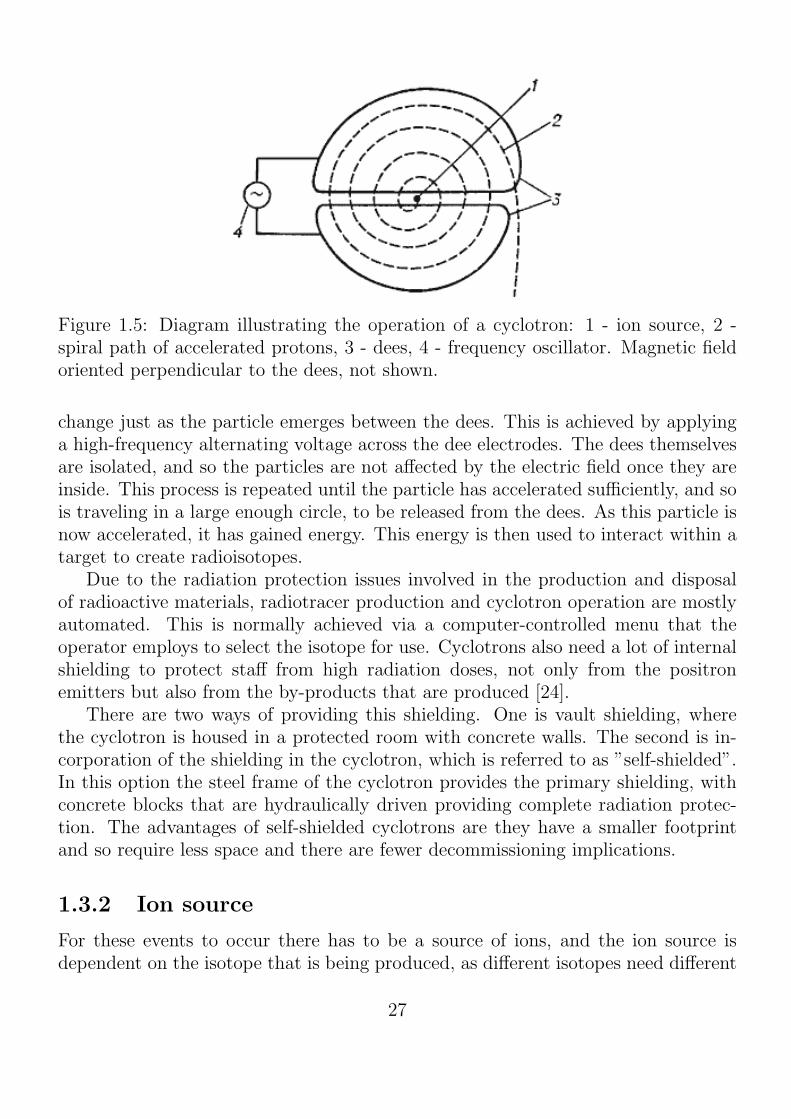
Figure 1.5: Diagram illustrating the operation of a cyclotron: 1 - ion source, 2 -spiral path of accelerated protons, 3 - dees, 4 - frequency oscillator. Magnetic fieldoriented perpendicular to the dees, not shown.

change just as the particle emerges between the dees. This is achieved by applyinga high-frequency alternating voltage across the dee electrodes. The dees themselvesare isolated, and so the particles are not affected by the electric field once they areinside. This process is repeated until the particle has accelerated sufficiently, and sois traveling in a large enough circle, to be released from the dees. As this particle isnow accelerated, it has gained energy. This energy is then used to interact within atarget to create radioisotopes.

Due to the radiation protection issues involved in the production and disposalof radioactive materials, radiotracer production and cyclotron operation are mostlyautomated. This is normally achieved via a computer-controlled menu that theoperator employs to select the isotope for use. Cyclotrons also need a lot of internalshielding to protect staff from high radiation doses, not only from the positronemitters but also from the by-products that are produced [24].

There are two ways of providing this shielding. One is vault shielding, wherethe cyclotron is housed in a protected room with concrete walls. The second is in-corporation of the shielding in the cyclotron, which is referred to as ”self-shielded”.In this option the steel frame of the cyclotron provides the primary shielding, withconcrete blocks that are hydraulically driven providing complete radiation protec-tion. The advantages of self-shielded cyclotrons are they have a smaller footprintand so require less space and there are fewer decommissioning implications.

1.3.2 Ion source

For these events to occur there has to be a source of ions, and the ion source isdependent on the isotope that is being produced, as different isotopes need different

27

interactions between target and particle. The ion source is a small chamber in thecenter of the cyclotron that produces either negative or positive ions, dependingon the configuration. These particles are attracted into the dees by electrostaticattraction [23]. Negative hydrogen ions (H−) are produced by using a tungstenfilament to ionize hydrogen gas. The electrons are stripped off the H− particle usinga carbon foil, leaving an accelerated proton to interact within the target.

The exiting charged particles are directed to the required target using a deviatingelectromagnet. This means that different isotopes can be produced using the samecyclotron depending on the target used.

1.3.3 Positron emitter production

Once charged particles exit the cyclotron, they can go on to produce positron emit-ters by interacting with a target. The isotope that is produced depends on the typedof charged particle that has been accelerated and the material from which the targetis made.

While many different radioactive isotopes can be produced in the cyclotron, inorder to be suitable for PET imaging they must have the following properties:

• Emit positrons when they decay;

• Have an appropriate half-life time;

• Be capable of being synthesized into a pharmaceutical to produce a usefultracer for studies in humans.

When targets of stable elements are irradiated by placing them in the beam ofaccelerated particles, the particles interact with the nuclei within the target andnuclear reactions take place. The following nuclear reactions induced by a proton p,on a target A

ZX can be given by:

AZX + p → A

Z+1Y + n (1.1)

AZX + p → A−3

Z−1Y + α (1.2)

For example, 18F is produced by proton bombardment 18O-enriched water:

18O + p → 18F + n (1.3)

A proton interacts with the 14N and produces α particle and 11C:

14N + p → 11C + α (1.4)

28

13N is produced by proton bombardment of distilled water:

16O + p → 13N + α (1.5)

A reaction induced by a deuteron d, on a target AZX can be given by:

AZX + d → A+1

Z+1Y + n (1.6)

For instance, 15O radionuclide production:

14N + d → 15O + n (1.7)

Nuclide Emax, MeV T1/2, minRange in water, mmMax Mean

11C 0.959 20.4 4.1 1.113N 1.197 9.96 5.1 1.515O 1.738 2.03 7.3 2.518F 0.633 109.8 2.4 0.6

Table 1.1: Properties of the main positron-emitting nuclides of interest in PET [25].

1.4 Physics in PET

1.4.1 Positron decay

Positron emission from the nucleus is radioactive decay described by:

11p

+ → 10n+ 0

1β+ + νe (1.8)

The general equation for positron decay from an atom is:

AZX → A

Z−1Y + 01β

+ + ν +Q(e+) (1.9)

where Q(e+) is kinetic energy of the emitted positron. The atom X is proton-richand achieves stability by converting a proton to a neutron. The positive charge iscarried away with the positron. As the daughter nucleus has an atomic number oneless than the parent, one of the orbital electrons must be ejected from the atom tobalance charge. This is often achieved by a process known as internal conversion,where the nucleus supplies energy to an orbital electron to overcome the bindingenergy and leave it with residual kinetic energy to leave the atom.

29

The emitted positron will have an initial energy and the energy spectrum isa continuum of values up to a maximum. After emission from the nucleus, thepositron loses kinetic energy by interactions with the surrounding matter. Thepositron interacts with other nuclei as it is deflected from its original direction byone of four types of interaction:

• Inelastic collisions with atomic electrons, which is the predominant mechanismof loss of kinetic energy,

• Elastic scattering with atomic electrons, where the positron is deflected butenergy and momentum are conserved,

• Inelastic scattering with a nucleus, with deflection of the positron and oftenwith the corresponding emission of Bremsstrahlung radiation,

• Elastic scattering with a nucleus where the positron is deflected but does notradiate any energy.

Figure 1.6: Annihilation radiation is produced subsequent to a positron being ejectedfrom the nucleus. The positron travels a finite distance, losing energy by interactionwith other electrons and nuclei as it does, until it comes to rest and combines(annihilates) with an electron to give rise to two photons, each equivalent to therestmass energy of the particles. The two photons are approximately anti-collinearand it is this property that is used to localize events in PET.

As the positron passes through matter it loses energy constantly in ionizationevents with other atoms or by radiation after an inelastic scattering. Both of thesesituations will induce a deflection in the positron path, and thus the positron takes

30

an extremely tortuous passage through matter. Due to this, it is difficult to estimatethe range of positrons based on their energy alone, and empirical measurements areusually made to determine the mean positron range in a specific material.

The positron eventually combines with an electron when both are essentially atrest. A metastable intermediate species called positronium may be formed by thepositron and electron combining. Positronium is a non-nuclear element composedof the positron and electron. Positronium formation occurs with a high probabilityin gases and metals, but only in about one-third of cases in water or human tissuewhere direct annihilation of the electron and the positron is more favorable [25].Positronium can exist in either of two states, parapositronium (spin = +1/2, life-time in vacuum τ = 100 ps) or orthopositronium (spin = +3/2, life-time in vacuumτ = 125 ns). Approximately three-quarters of the positronium formed in vacuum isorthopositronium.

Positron emission from the nucleus, with subsequent annihilation, means that thephoton-producing event (the annihilation) occurs outside the radioactive nucleus.The finite distance that positrons travel after emission contributes uncertainty tothe localization of the decaying nucleus (the nucleus is the species that we wish todetermine the location of in positron tomography, not where the positron eventuallyannihilates). The uncertainty due to positron range is a function that increases withincreasing initial energy of the positron. For a high-energy positron such as 82Rb(Emax = 3.4 MeV), the mean range in water is around 5.9 mm. Table 1.1 shows somecommonly used positron emitting nuclides and associated properties. When thepositron and electron eventually combine and annihilate electromagnetic radiationis given off. The most probable form that this radiation takes is of two photonsof 0.511 MeV (the rest-mass equivalent of each particle) emitted at approximately180 to each other, however, three photons can be emitted (< 1% probability). Thephotons are emitted in opposed directions to conserve momentum, which is close tozero before the annihilation.

Many photon pairs are not emitted strictly at 180, however, due to non-zeromomentum when the positron and electron annihilate. This fraction has been es-timated to be as high as 65 % in water. This contributes a further uncertainty tothe localization of the nuclear decay event of 0.5 FWHM from strictly 180, whichcan degrade resolution by a further 1.5 mm (dependent on the distance between thetwo coincidence detectors) (see Fig. 1.7). This effect, and the finite distance trav-eled by the positron before annihilation, places a fundamental lower limit of spatialresolution that can be achieved in positron emission tomography [26].

31

Figure 1.7: Acollinearity introduces a positional error in PET imaging.

1.4.2 Interaction of high energy photons with matter

High-energy photons interact with matter by three main mechanisms, dependingon the energy of the electromagnetic radiation. These are the photoelectric effect,the Compton effect, and pair production (the photon must have higher energy thanthe sum of the rest mass energies of an electron and positron (2 × 0.511 MeV =1.022 MeV) for the production to occur). In addition, we have considered the follow-ing optical photon processes. For optical photons (250 - 700 nm wavelength) thereare other mechanisms such as elastic Rayleigh scattering, absorption and mediumboundary interactions. The Geant4 catalog of processes at optical wavelengths in-cludes all of them. The optical properties of the medium which are key to theimplementation of these types of processes are stored as entries in a properties tablelinked to the material in question. They may be expressed as a function of thephoton’s wavelength.

1.4.2.1 Photoelectric effect

The photoelectric effect is an interaction of photons with orbital electrons in anatom. This is shown in Fig. 1.8 [25]. The photon transfers all of its energy to theelectron. Some of the energy is used to overcome the binding energy of the electron,and the remaining energy is transferred to the electron in the form of kinetic energy.The photoelectric effect most probably occurs with an inner shell electron. As the

32

electron is ejected from the atom (causing ionization of the atom) a more looselybound outer orbital electron drops down to occupy the vacancy. In doing so it willemit radiation itself due to the differences in the binding energy for the differentelectron levels. This is a characteristic X-ray. The ejected electron is known asa photoelectron. Alternately, instead of emitting an X-ray, the atom may emit asecond electron to remove the energy and this electron is known as an Auger electron.This leaves the atom doubly charged. Characteristic X-rays and Auger electrons areused to identify materials using spectroscopic methods based on the properties ofthe emitted particles. The photoelectric effect dominates in human tissue at energiesless than approximately 100 keV. It is of particular significance for X-ray imaging,and for imaging with low-energy radionuclides. It has little impact at the energy ofannihilation radiation (511 keV), but with the development of combined PET/CTsystems, where the CT system is used for attenuation correction of the PET data,knowledge of the physics of interaction via the photoelectric effect is extremelyimportant when adjusting the attenuation factors from the X-ray CT to the valuesappropriate for 511 keV radiation.

Figure 1.8: The photon is absorbed by photoelectric effect.

1.4.2.2 Compton scattering

Compton scattering is the interaction between a photon and a loosely bound orbitalelectron. The electron is so loosely connected to the atom that it can be consideredto be essentially free. This effect dominates in human tissue at energies aboveapproximately 100 keV and less than ∼2 MeV. The binding potential of the electronto the atom is extremely small compared with the energy of the photon, such thatit can be considered to be negligible in the calculation. After the interaction, thephoton undergoes a change in direction and the electron is ejected from the atom.

33

The energy loss by the photon is divided between the small binding energy of theenergy level and the kinetic energy imparted to the Compton recoil electron. Theenergy transferred does not depend on the properties of the material or its electrondensity (Fig. 1.9). The energy of the photon after the Compton scattering can becalculated from the Compton equation:

E′

γ =Eγ

1 +Eγ

m0c2(1− cos θc)

(1.10)

Figure 1.9: In Compton scattering, part of the energy of the incoming photon istransferred to an atomic electron. This electron is known as the recoil electron. Thephoton is deflected through an angle proportional to the amount of energy lost.

From consideration of the Compton equation it can be seen that the maximumenergy loss occurs when the scattering angle is 180 (cos(180) = - 1), i.e., the photonis back-scattered. A 180 back-scattered annihilation photon will have an energy of170 keV and emitted electron has an energy of 341 keV, this is the energy of the,so-called, Compton edge. Compton scattering is not equally probable at all energiesor scattering angles. The probability of scattering is given by the Klein-Nishinaequation [27]:

dσ

dΩ= Zr20

(

1

1 + α(1− cos θc)

)2(1 + cos 2θ

2

)(

1 +α2(1− cos θc)

2

(1 + cos 2θc)(1 + α1− cos θc)

)

(1.11)where dσ/dΩ is the differential scattering cross-section, Z is the atomic number

of the scattering material, r0 is the classical electron radius, and α = Eγ/m0c2. For

positron annihilation radiation (where α = 1) in tissue, this equation can be reducedfor first-order scattered events to give the relative probability of scatter as:

34

dσ

dΩ=

(

1

2− cos θc

)2(

1 +(1− cos θc)

2

(2− cos θc)(1 + cos 2θc)

)

(1.12)

The induced shape of the electron energy spectrum, as simulated by the GEANT4software, will be discussed in the Section 3.2.

1.4.2.3 Pair production

Another mechanism for photons to interact with matter is by pair production. Whenphotons with energy greater than 1.022 MeV (twice the energy equivalent to the restmass of an electron) pass in the vicinity of a nucleus it is possible that they willspontaneously convert to electron-positron pair. This direct electron pair productionin the Coulomb field of a nucleus is the dominant interaction mechanism at highenergies (Fig. 1.10). Above the threshold of 1.022 MeV, the probability of pairproduction increases as energy increases. At 10 MeV, this probability is about 60%.Any energy left over after the production of the electron-positron pair is sharedbetween the particles as kinetic energy and recoil energy nucleus, with the positronhaving slightly higher kinetic energy than the electron as the interaction of theparticles with the nucleus causes an acceleration of the positron and a deceleration ofthe electron. The process of pair production demonstrates a number of conservationlaws.

Figure 1.10: The pair production process is illustrated. As a photon passes inthe vicinity of a nucleus spontaneous formation of positive and negatively chargedelectrons can occur. The threshold energy required for this is equal to the sum ofthe rest masses for the two particles (1.022 MeV).

35

Since in the PET the photon energy is limited to the 511 keV the pair productionis not relevant and could be omitted in the simulation.

1.4.2.4 Attenuation of photons

Calculations of photon interactions are given in terms of atomic cross sections (σ)with units of [cm2/atom]. An alternative unit, often employed, is to quote the crosssection for interaction in [barns/atom], where 1 [barn] = 10−24[cm2]. The totalatomic cross section is given by the sum of process relevant for the photons withenergies less than 511 keV:

σtot = σpe + σincoh + σcoh, (1.13)

where the cross sections are for the photoelectric effect (pe), incoherent Comptonscattering (incoh), coherent (Rayleigh) scattering (coh). Values for attenuation coef-ficient are often given as mass attenuation coefficients (µ/ρ) with units of [cm2·g−1].The reason for this is that this value can be converted into a linear attenuationcoefficient (µl) for any material simply by multiplying by the density (ρ) of thematerial:

µ1[cm−1] = µ/ρ[cm2 · g−1]ρ[g · cm−3]. (1.14)

The mass attenuation coefficient is related to the total cross section by:

µ/ρ[cm2 · g−1] =σtotu[g]A

, (1.15)

where u[g] = 1.661 × 10−24[g] is the atomic mass unit (1/NA where NA is Avo-gadro’s number) defined as 1/12th of the mass of an atom of 12C, and A is therelative atomic mass of the target element [28].

We have seen that the primary mechanism for photon interaction with matterat energies around 0.5 MeV is by a Compton interaction. The result of this formof interaction is that the primary photon changes direction (i.e., is ”scattered”) andloses energy. In addition, the atom where the interaction occurred is ionized. Fora well-collimated source of photons and detector, attenuation takes the form of amono-exponential function, i.e.,

Ix = I0e−µx (1.16)

where I represents the photon beam intensity, the subscripts ”0” and ”x” referrespectively to the unattenuated beam intensity and the intensity measured througha thickness of material of thickness x, and µ refers to the attenuation coefficient ofthe material (units: cm−1). Attenuation is a function of the photon energy and

36

the electron density (Z number) of the attenuator. The attenuation coefficient isa measure of the probability that a photon will be attenuated by a unit length ofthe medium. For example, the linear attenuation coefficient for a water is about0.096 cm−1 [12] (see Fig. 1.11).

Figure 1.11: Linear attenuation coefficient for a water [12].

Positron emission possesses an important distinction from single-photon mea-surements in terms of attenuation. Consider the count rate from a single photonemitting point source of radioactivity at a depth, a, in an attenuating medium oftotal thickness, D (see Fig. 1.12). The count rate C observed by an external detectorA would be:

Ca = C0e−µa. (1.17)

where C0 represents the unattenuated count rate from the source, and µ is theattenuation coefficient of the medium (assumed to be a constant here). Clearly thecount rate changes with the depth a. If measurements were made of the source fromthe 180 opposed direction the count rate observed by detector B would be:

Cb = C0e−µ(D−a), (1.18)

where the depth b is given by (D − a). The count rate observed by the detectorswill be equivalent when a = b. Now consider the same case for a positron-emitting

37

Figure 1.12: Detectors A and B record attenuated count rates arising from the sourcelocated a distance a from detector A and b from detector B. For each positron anni-hilation, the probability of detecting both photons is the product of the individualphoton detection probabilities. Therefore, the combined count rate observed is in-dependent of the position of the source emitter along the line of response. The totalattenuation id determined by the total thickness (D) alone.

source, where detectors A and B are measuring coincident photons. The count rateis given by the product of the probability of counting both photons and will be:

C = (C0e−µa)× (C0e

−µ(D−a)) = C0(e−µa × e−µ(D−a)) = C0e

−µ(a+(D−a)) = C0e−µD.(1.19)

which shows that the count rate observed in an object only depends on the totalthickness of the object, D; i.e., the count rate observed is independent of the positionof the source in the object. Therefore, to correct for attenuation of coincidencedetection from annihilation radiation one measurement, the total attenuation pathlength (−µD), is all that is required.

For example, for a D = 20 cm (typical size of phantom used in PET), the fluxof the 511 keV photons will be attenuated by a factor of 6.8 in water. As wewill see in the Section 2.6.2 the attenuation plays an important role during imagereconstruction and need to be taken into account.

1.4.3 Interaction of optical photons with matter

A photon is considered to be optical when its wavelength is much greater than thetypical atomic spacing. In GEANT4 optical photons are treated as a class of particledistinct from their higher energy gamma cousins. This implementation allows thewave-like properties of electromagnetic radiation to be incorporated into the opticalphoton process. Because this theoretical description breaks down at higher energies,there is no smooth transition as a function of energy between the optical photonand gamma particle classes.

38

1.4.3.1 Rayleigh and Mie scattering

Rayleigh process is defined only for low energy photons because at high energies, thecross-section of the Rayleigh scattering is very small and usually can be neglected.For these process, no energy is transferred to the target, all the electrons of the atomcontribute in a coherent way (this process is also called coherent scattering). Thedirection of the photon is the only modified parameter. Atoms are not excited orionized. The intensity of the scattered light is proportional to 1/λ4 [29].

Mie Scattering (or Mie solution) is an analytical solution of Maxwell’s equationsfor scattering of optical photons by spherical particles. It is significant only whenthe radius of the scattering object is of order of the wave length. The analyticalexpressions for Mie scattering are very complicated since they are a series sumof Bessel functions. Geant4, thus, GATE follows one common implementation byHenyey-Greenstein approximation [30]:

dσ

dΩ= r

dσ

dΩ(σf , gf) + (1− r)

dσ

dΩ(σb, gb), (1.20)

where dΩ = d cos(θ)dθ, θb = π− θf and r is the ratio factor between the forwardangle and backward angle.

1.4.3.2 UNIFIED model

Medium boundary interactions in Geant4 and GATE employ the UNIFIEDmodel [31].It applies to dielectric-dielectric interfaces and tries to provide a realistic simulation,which deals with all aspects of surface finish and reflector coating (see Fig. 1.13).The surface may be assumed as smooth and covered with a metallized coating repre-senting a specular reflector with given reflection coefficient, or painted with a diffusereflecting material where Lambertian reflection occurs. The surfaces may or may notbe in optical contact with another component and most importantly, one may con-sider a surface to be made up of micro-facets with normal vectors that follow givendistributions around the nominal normal for the volume at the impact point. Forvery rough surfaces, it is possible for the photon to inversely aim at the same surfaceagain after reflection of refraction and so multiple interactions with the boundaryare possible within the process itself.

1.4.4 Charged particle interaction with matter

The energetic charged particles such as α particles and β particles, while passingthrough matter, lose their energy by interacting with the orbital electrons of theatoms in the matter. In these processes, the atoms are ionized in which the electronin the encounter is ejected or the atoms are excited in which the electron is raised to

39

Figure 1.13: The UNIFIED model provides for a range of different reflection mech-anisms [30].

a higher energy state. In both excitation and ionization processes, chemical bonds inthe molecules of the matter may be ruptured, forming a variety of chemical entities.The range of a charged particle depends on the energy, charge, and mass of theparticle as well as the density of the matter it passes through. It increases withincreasing of charge and energy.

1.4.4.1 Cherenkov radiation

The phenomenon of the Cherenkov radiation was discovered experimentally byCherenkov and theoretically by Frank and Tamm in the 1930s in the Union ofSoviet Socialist Republics and for this work scientists were awarded the Nobel Prizein 1958.

The famous equation that defines the opening angle θ of the cone for generatedCherenkov photons (see Fig. 1.14) in the medium with refractive index n is [32]:

40

β =1

cos θ · n, (1.21)

where β = v/c, and v is the velocity of the charged particle, c is the speed of light.From this equation it is evident that in case β ∼ 1, the threshold value βmin below

which no radiation can be emitted is inversely proportional to refractive index ofthe medium:

βmin =1

n. (1.22)

Therefore, for our Cherenkov tomograph we consider the lead fluoride crystal, whichis one of the best candidate for Cherenkov production with high refractive index ofabout 1.82 (for more details see Section 3.2).

Figure 1.14: The Cherenkov radiation is often described as being analogous to theshock wave emitted in the acoustic range by a projectile or plane moving throughair faster than the speed of sound or to the bow wave created by a boat movingacross water. Cerenkov photons occur when a charged particle moves through adispersive medium faster than velocity of the light in that same medium. Cherenkovlight is emitted on the surface of a cone with maximum opening angle of θmax =arccos( 1n). Thus, any charged particle with appropriate speed will produce theCherenkov radiation. When the particle has slowed below the local speed of light,the radiation ceases and the emission cone has collapsed to zero. The photonsproduced by this process have an inherent polarization perpendicular to the cone’ssurface at production.

The number of the emitted optical photons N depends on the photon wavelength

41

λ as [33]:∂2N

∂x∂λ= 2πα

(

1−1

β2n2

)

1/λ2, (1.23)

where α = 1/137 is the fine structure constant. Unlike the fluorescence oremission spectra, the Cherenkov radiation spectrum given by the above formula, iscontinuous and its density is inversely related to the wavelength squared. Therefore,the number of optical photons increases as the wavelength decreases. That explainswhy the Cherenkov radiation seems blue and mostly in UV range and at the sametime this peculiarity should be take into account when different optical mediums areconsidering. Significant number of photons can be lost because of the transparencyof the materials.

The validity of Cherenkov’s observations and of equation 1.21 was strikinglyconfirmed by Collins and Resling [34]. Cherenkov was the first, who suggested thatthe radiation might be used for detection of the charged particles. This processis much faster in comparison with scintillation, and with recent developments inelectronics and detection becomes more and more interesting for medical physicsapplication.

The GATE allows to simulate Cherenkov process. In this modeling the time andposition of Cherenkov photon emission are calculated from quantities known at thebeginning of a charged particle’s step. The step is assumed to be rectilinear evenin the presence of a magnetic field. The step size can be limited by specifying amaximum (average) number of Cherenkov photons created during the step (usingthe SetMaxNumPhotonsPerStep method). The actual number generated will nec-essarily be different due to the Poissonian nature of the production. In the presentimplementation, the production density of photons is distributed evenly along theparticle’s track segment, even if the particle has slowed significantly during the step.We discuss the simulation result on the number of the produced Cherenkov photonsin the detector and the corresponding wavelength spectrum in the Section 3.2.

42

Chapter 2

Instrumentation in PET

2.1 Main characteristics of the detectors for PET

The physical characteristics of PET tomographs can be specified in terms of parame-ters such as transverse (in-plane) and axial spatial resolution, sensitivity, countrate capability, scatter fraction and image uniformity. Measurements are madewith phantoms such as line sources and 20 cm diameter uniform cylinders ac-cording to standards defined by the National Electrical Manufacturers Association(NEMA) [35]. These measurements reflect the performance of the scanner and pro-vide a basis on which to compare different tomographs. However, it is difficult torealistically evaluate overall scanner performance based on comparisons of a singleparameter such as spatial resolution or maximum count rate.

2.1.1 Sensitivity

Scanner’s sensitivity represents its ability to detect the coincident photons emittedfrom inside the scanner FOV and defined as number of counts per unit time detectedby the device (i.e., [cps/µCi] or [cps/kBq]) [25]. In particular, this characteristicdepends on two parameters of the scanner: fraction of the total solid angle coveredby it over the imaging field and the stopping efficiency of the detectors for 511 keVphotons. Based on the above factors discussed, the sensitivity S of a single ringPET scanner can be expressed as [36]:

S =A · ε2 · e−µd · 3.7× 104

4πr2[cps/µCi], (2.1)

where A is detector area seen by a point source to be imaged in the center FOV, εis detector efficiency, µ is a linear attenuation coefficient of 511 keV photons in thedetection material with thickness d, and r is the radius of the ring of the scanner.The proportionality to ε2 arises from the two detectors with efficiency ε, i.e., ε× ε.

43

Therefore, small-diameter PET scanners (i.e., small-animal PET scanners de-scribed in the Section 1.2) have higher sensitivity. Another way to improve sensi-tivity is to increase the axial FOV (i.e. project EXPLORER for total-body PETscanning with announced axial FOV of 2 m [37]).

The stopping efficiency of the PET detector is related to the type of detectorbeing used. The geometric factor depends on the distance between the source and thedetector, the diameter of the ring and the number of detectors per ring. Increasingthe distance between the detector and the source reduces the solid angle and thusdecreases the geometric efficiency of the scanner and vice versa and in the same timeincreasing the diameter of the ring decreases the solid angle subtended by the sourceat the detector, thus, reducing the geometric efficiency and in turn the sensitivity.Also the sensitivity increases with increasing number of rings in the scanner. Westudy this effect in the Section 4.2 while we increase scanner diameter from 81 cmto 91 cm.

For an extended source at the center of such scanners, the geometric efficiencyis approximated as w/2r, where w is the axial width of the detector element and ris the radius of the ring. Thus, the sensitivity of the scanner is highest at the centerof the axial FOV and gradually decreases toward the periphery.

As it known, for typical PET scanners, there are also multiple rings and eachdetector is connected in coincidence with as many as half the number of detectorson the opposite side in the same ring as well as with detectors in other rings. Thus,the sensitivity of multi-ring scanners will increase with the number of the detectorrings.

In addition, sensitivity of the PET machine increases as the square of the detec-tor efficiency, which depends on the scintillation decay time (for scintillators) andstopping power of the detector.

We estimated the sensitivity of the scanner during image reconstruction andtypical distribution is shown in Fig. 2.1.

2.1.2 Energy resolution

Typically, radiation detectors convert the deposited energy into a measurable elec-trical signal or charge. The integral of this signal is then proportional to the totalenergy deposited in the detector by the radiation. The ability of the radiation de-tector to accurately measure the deposited energy is of paramount importance formost of its uses. This accuracy is characterized by the width of the photopeak inthe energy spectrum, and is referred to as the energy resolution of the detector.

In PET, the development of the 3D volumetric acquisition and improvements inthe detector energy resolution have allowed the implementation of scatter correctionsbased on the analysis of the photon energy. The scatter correction consist of the

44

Figure 2.1: Sensitivity of the scanner for image reconstruction calculated using thecode CASToR.

subtraction of a fraction of the Compton data from the photopeak data.The conventional tomographs based on the BGO scintillator crystals have an

energy resolution of about 25 %, and are usually operated with an energy thresholdin the range 250-350 keV [38]. Many small-angle Compton scatters involve littleenergy loss and are therefore accepted within the wide energy window of BGO.Another inorganic scintillators such as lutetium oxyorthosilicate (LSO) [39] haveimproved light output and better energy resolution that may help reduce the scatterfraction. Nevertheless, the energy resolution of LSO will not be as good as that ofNaI and even an energy resolution of 10-12 % still results in a scatter fraction in 3D ofaround 30 %. Decreasing the lower level discriminator (LLD) setting from 380 keV to150 keV increases unscattered counts (by about 20 %) as well as increasing scatteredevents. Improved energy resolution from better scintillation materials reaches 8-10 %(FWHM) at 511-keV [26].

Therefore, scatter will be always present and methods dealing with it will berequired. The incorporation of non-energy based methods may help in improving of

45

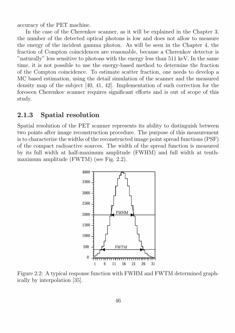
accuracy of the PET machine.In the case of the Cherenkov scanner, as it will be explained in the Chapter 3,

the number of the detected optical photons is low and does not allow to measurethe energy of the incident gamma photon. As will be seen in the Chapter 4, thefraction of Compton coincidences are reasonable, because a Cherenkov detector is”naturally” less sensitive to photons with the energy less than 511 keV. In the sametime, it is not possible to use the energy-based method to determine the fractionof the Compton coincidence. To estimate scatter fraction, one needs to develop aMC based estimation, using the detail simulation of the scanner and the measureddensity map of the subject [40, 41, 42]. Implementation of such correction for theforeseen Cherenkov scanner requires significant efforts and is out of scope of thisstudy.

2.1.3 Spatial resolution

Spatial resolution of the PET scanner represents its ability to distinguish betweentwo points after image reconstruction procedure. The purpose of this measurementis to characterize the widths of the reconstructed image point spread functions (PSF)of the compact radioactive sources. The width of the spread function is measuredby its full width at half-maximum amplitude (FWHM) and full width at tenth-maximum amplitude (FWTM) (see Fig. 2.2).

Figure 2.2: A typical response function with FWHM and FWTM determined graph-ically by interpolation [35].

46

2.1.4 Timing resolution

The timing resolution of a PET detector describes how precisely could be measuredthe gamma conversion time in the detector. It has several contribution related to thecrystal geometry, electronics performance and characteristic time of the signal gener-ation. The timing resolution of a PET detector is important because it involves thedetection of two photons originating from a single coincident event. Since the timingresolution represents the variability in the signal arrival times for different events, itneeds to be properly accounted for when detecting coincident events. Fig. 2.3 givesa schematic representation of two detectors set up to measure coincident photonsbeing emitted from a point equidistant from the two detectors.

The coincidence circuitry, however, generates a narrow trigger pulse when thedetector signals cross a certain fixed fraction of their individual amplitudes. Attime t1, signal A triggers pulse 1 which also produces a coincidence time windowof a predetermined width, 2τ . Signal B, depending upon the timing resolution ofthe detector, will trigger at a later time, t2. Depending upon the difference t2 - t1,the start of pulse 2 may or may not overlap with the Coincidence window. Fordetectors with poor timing resolution, a large value for 2τ needs to be used in orderto detect most of the valid coincidence events [43].

In a PET scanner, the two coincident photons will be emitted from anywherewithin the scanner FOV and so the distance traveled by each of them before in-teraction in the detectors will be different. For a typical whole-body scanner, thisdistance can be as large as the scanner diameter (about 100 cm). Using the value ofspeed of light (c = 3× 108 m/s), one can calculate an additional maximum timingdifference of about 3-4 ns between the two signals (the photons travel 1 m in 3.3 ns).As a result, the coincidence timing window (2τ) of a PET detector needs to be in-creased even more than the requirements of the timing resolution. The consideredCherenkov detector are design to be very fast. However, the coincidence timing win-dow cannot be reduced to less than 3-4 ns (in a whole-body scanner geometry) dueto the difference in arrival times of two photons emitted at the edge of the scannerfield of view, as this would restrict the transverse field of view.

For foreseen Cherenkov whole-body TOF-PET scanner with inner diameter ofthe ring 81 cm we implemented 4.0 ns coincidence window.

47

Figure 2.3: Signal A results in a trigger pulse 1. Similarly, signal B results in atrigger pulse 2. A coincidence (AND) circuit then checks for coincidence betweenthe pulse 2 and the coincidence window of width ∆t [25].

48

2.2 Conventional approach: scintillators

Although many scintillation materials have been investigated, only several of themhave been commonly used in PET technology [44]. The use of the scintillator de-tector in PET is based on its properties, such as stopping power of the detector,density, scintillation decay time, light yield and energy resolution at 511 keV, seeTab. 2.1.

Detectors Effective Density, Scintillation Photon Linear attenuationatomic no ρ decay time, yield coefficient, µ resolution

Zeff [g/cm3] [ns] [photon/per keV] [cm−1] at

NaI(Tl) 51 3.67 250 38 0.34BGO 75 7.13 300 9 0.96BaF2 54 4.89 0.6 2 0.44GSO 59 6.71 50 10 0.67LSO 66 7.40 40 29 0.87LYSO 65 7.20 50 25 0.87LaBr3 49.6 5.3 5 (35) 61 0.47

Table 2.1: Main properties of the solid scintillators have application in PET [44, 45].

The mean distance the photon travels through detector material until completeenergy deposition depends on the density and effective atomic number (Zeff) of thedetector.

The scintillation decay time arises when a gamma ray interacts with an atom ofthe detector material, and the atom is excited to a higher energy level, which laterdecays to the ground state, emitting visible light [46]. The scintillation efficiencyof any scintillator is defined as the fraction of all incident particle energy which isconverted into visible light.

The scintillation decay time is the time required for scintillation emission todecrease to e−1 of its maximum and consist of fast and slow components. In mostorganic scintillators the decay time is a few nanoseconds, for inorganic materials itis 40 ns and more.

Photon yield or light output is the ability of conversion of ionizing radiation intolight energy, and it can be defined as the number of visible photons produced in thebulk of scintillator per energy unit keV. A high-light-output detectors generate well-defined light pulse, and as a result better energy resolution. The intrinsic energyresolution is affected by inhomogeneities in the crystal structure of the detector

49

and random variations in the production of light in it. The energy resolutionsat 511 keV in different detectors vary from 2.9 to 20%, using routine integrationtime for pulse formation, which runs around a few microseconds. However, in PETimaging, the integration time is a few hundred nanoseconds in order to excluderandom coincidences, and the number of photoelectrons collected for a pulse issmall, thus degrading the energy resolution. Consequently, the detectors in PETscanners have relatively poorer energy resolution [44].

2.3 Non-conventional approaches

Besides scintillation crystals, another detection materials such as liquids and gasescan be apply for non-conventional approach in PET. For example, project of theCaLIPSO group at IRFU is development of the brain-scanning PET device withTOF capability using an innovative liquid TriMethylBismuth (TMBi), the chemi-cal formula is Bi(CH3)3, as the detection medium [47]. The TMBi’s coincidencephotoelectric efficiency is twice the value of the LSO/LYSO crystals. Thus, themeasured detection efficiency of 85 % for the 511 keV gamma that undergo a pho-toelectric conversion in TMBi, a promising feature for a potential high resolutionPET-scanner.

The proportional chamber works on the principle of detecting the ionizationproduced by radiation as it passes through a gas chamber. A high electric field isapplied within this chamber that results in an acceleration of the ionization electronsproduced by the radiation. Subsequently, these highly energetic electrons collidewith the neutral gas atoms resulting in secondary ionizations. Hence, a cascadeof electrons is eventually collected at the cathode after some energy deposition bythe incident radiation. Typically, inert gases such as xenon are used for detectingphotons. The cathode normally consists of a single thin wire, but a fine grid ofwires can be utilized to measure energy deposition as a function of position withinthe detector. Such position-sensitive Multi-wire Proportional Chambers (MWPC)have been used in high-energy physics for a long time, and PET scanners have beendeveloped based upon such a detector [48, 49, 50]. However, the disadvantage ofthese detectors for use in PET is the low density of the gas, leading to a reducedstopping efficiency for 511 keV photons, as well as poor energy resolution.

Several groups work with Cherenkov light detection for PET [51, 52, 15, 53] butstill the main limitation factor is low detection efficiency.

2.4 Data Acquisition. Types of coincidences

An event in PET is regarded as valid (or good) if:

50

1. two photons are detected within a predefined electronic time window knownas the coincidence window,

2. the subsequent LOR formed between them is within a valid acceptance angleof the tomograph,

3. the energy deposited in the crystal by both photons is within the selectedenergy window (for conventional scanners).

The various coincidence events that can be recorded in PET are divided by threecategories and shown diagrammatically in Fig. 2.4.

The prompt count rate is given by the sum of the true plus random plus scat-tered event rates.

A true coincidence is an event that derives from a single positron-electron an-nihilation labeled with yellow star on the scheme, Fig. 2.4a. The two annihilationphotons both reach detectors on opposing sides of the tomograph without any sig-nificant scattering in the subject and are recorded within the coincidence timingwindow.

Scattered events arise when one or both of the photons from a single positronannihilation detected within the coincidence timing window have undergone a Comp-ton interaction, labelled by blue star in the Fig. 2.4b. Compton scattering causesa loss in energy of the photon and change in direction of the photon. The fractionof scattered events is not a function of count rate, but is constant for a particularobject and radioactivity distribution.

A random (or accidental) coincidence occurs when two different nuclei decayat approximately the same time. After annihilation of both positrons, four photonsare emitted. Two of these photons from different annihilations are counted withinthe timing window and are considered to have come from the same positron, whilethe other two are lost, i.e. black arrows in the Fig. 2.4c and Fig. 2.4d.

Multiple events are similar to random events, except that several events fromtwo annihilations are detected within the coincidence timing window. Due to theambiguity in deciding which pair of events arises from the same annihilation, theevent can be disregarded or saved. GATE allows to simulate nine coincidence policies(see Tab. 4.2).

The GATE software propose to chose one of the predefined coincidence poli-cies for the coincidence sorter from the single detection. The following policies areavailable [54]:

• takeAllGoods: all possible pairs of the ”good” singles inside a specified timewindow and for each pair register a coincidence are considered;

• takeWinnerOfGoods: only the good pair with the highest energy is considered;

51

(a) (b)

(c) (d)

Figure 2.4: The yellow star indicates a positron annihilation vertex. The greenarrow is a true coincidence (a), only one useful signal for PET imaging. A scatterevent (b) is another type of possible coincidences, where one or both of photonsundergo a Compton interaction (a vertex of the Compton scattering is indicatedby blue star). A random coincidence (c) corresponds two independent annihilationsbut only two photons from four are detected within coincidence window, partiallythis effect can be reduced by adding shielding around the scanner, thus, the numberof random coincidences from out axial field-of-view (FOV) will be decreased (d).In case of scattered events and random events, mis-assigned lines of response areindicated by dashed lines. Non-detected photons are shown by black arrows.

• takeWinnerIfIsGood: if the pair with the highest energy is good, take it,otherwise, kill the event;

52

• takeWinnerIfAllAreGoods: if all pairs are goods, take the one with the highestenergy;

• keepIfOnlyOneGood: if exactly one pair is good, keep all the multi-coincidence;

• keepIfAnyIsGood: if at least one pair is good, keep all the multi-coincidence

• keepIfAllAreGoods: if all pairs are goods, keep all the multi-coincidence;

• killAllIfMultipleGoods: If more than one pairs is good, the event is seen as areal ”multiple” and thus, all events are killed;

• killAll: no multiple coincidences are accepted, no matter how many good pairsare presented.

”Good” means that a pair of singles are in coincidence and that the 2 singles areseparated by a number of blocks greater than or equal to the minSectorDifferenceparameter of the coincidence sorter.

Figure 2.5: Comparison of the behavior of the available multiple processing policies,for various multiple coincidences. The size of the star, as well as the number nextto it, indicates the energy level of the single event, i.e. event # 1 has more energythan single # 2. Image reproduced from [54]

2.5 Image reconstruction algorithms in PET

Tomographic image reconstruction techniques are commonly used to obtain 3D im-ages according to distribution of the radiotracer in a phantom or patient’s body.These images are obtained from sets of projection data that are recorded at differ-ent angles around the object. The quality of the image and the accuracy of theresulting data strongly depend on the reconstruction method. Although analyti-cal reconstruction methods (such as, for example, filtered back projection) are fast,they do not allow the reconstruction technique to model the SPECT or PET imaging

53

processes. This can be done when iterative methods are used, where an accuratereconstruction may include realistic modeling of the patient, the data acquisitionprocess, and the statistical nature of radioactive decay and photon interactions.

2.5.1 Analytical

Historically, for first image reconstructions was applied analytical approach. It is fastand simple in usage and is much less demanding than more complicated iterativealgorithms. However, there are many problems associated with its use. Becausethe method does not account for the statistical noise in the data and the high-frequency noise is enhanced by the ramp filter, smoothing filter must be included inthe reconstruction, which, in turn, degrades image spatial resolution.

For example, filtered back projection (FBP) is an analytical technique that is stillthe most commonly used method for image reconstruction in the clinical environ-ment. It employs a very simple model of the imaging process which assumes that thenumber of photons recorded in any given detector bin represents the sum of contri-butions from the activity located along a line perpendicular to the detector surface.Back-projection procedure redistributes all these photons (counts) back along a linedrawn through the images space. The points of intersection for the back-projectedlines are assumed to correspond to potential source locations. The projection andback-projection processes are shown schematically in Fig. 2.6. The back-projectionprocess results in a well-known star artifact around every source location unless theprojections are convolved with a sinc filter (ramp filter in Fourier domain) prior toback projection. FBP uses a simplistic model of the imaging process which does notallow for incorporation of any realistic data compensation techniques; therefore itsimages lack quantitative accuracy and often contain significant artifacts [55].

2.5.2 Iterative

Iterative reconstruction algorithms are more popular nowadays because of their bet-ter image quality they could propose compared to traditional analytical methods.A scheme in Fig. 2.7 represents the basic principle of this method.

At the first step we have to provide the scanning of the object and saving data.Then we start with uniform image of activity distribution, see Iteration # 1 in theFig. 2.8. Data are forward projected according to the scanner geometry, the resultingprojections are compared to the measured projections and the error-projection isused for correcting the estimate. The new estimate is then forward projected and thecomparison between estimated and measured projections yields the next correction.This loop is iterated until estimated and measured projections agree within theirstatistics, see Iteration # 2–10 in the Fig. 2.8.

54

Figure 2.6: Schematic view of analytical algorithm for image reconstruction inPET [55].

Improved availability of computing power and the introduction of fast algorithmshave introduced these methods in routine use. Spatial resolution which can beachieved in a PET image is principally limited by positron range and gamma raynon-collinearity. In addition, the width of the detection elements in the tomographdetermines the width of the coincidence response function and thus the image reso-lution.

2.5.3 CASToR platform for image reconstruction

For this study we use the CASToR reconstruction open-source platform for thetomographic 3D iterative reconstruction with TOF capability [56, 57]. This platformincludes several optimization algorithms, such as MLEM [58], OSEM, NEGML [59],AML (AB-EMML) [60] and Lanwdeber [61].

For image reconstruction we use MLEM (Maximum Likelihood ExpectationMaximization) optimization of list-mode data with continuous TOF information.

yi(tl) =∑

j

Aij(tl)λj + ri(tl) + si(tl), (2.2)

where yi(tl) is a number of counts detected in LOR i with TOF measurement,∆t = t1−t2 converted into delta length l along the LOR (shift from the LOR center);

55

Figure 2.7: Schematic view of iterative algorithm for image reconstruction inPET [55].

Aij is an element of the system matrix for voxel j and LOR i; λ is unknown activityto be reconstructed; ri and si is the number of random and scattered counts for eachLOR i.

∫ tlmax

tlmin

yi(tl)dtl = yi (2.3)

Aij(tl) =

∫

lvox

Gaussianσ,tl(l)dl (2.4)

An important moment is we can use the OSEM (Ordered Subset ExpectationMaximization).

2.6 Corrections

For obtaining a high quality final reconstructed emission images we have to applyseveral data corrections: normalization, correction for the attenuation, random andscatter events.

56

Figure 2.8: Evolution of the image with iterations.

2.6.1 Normalization

Nowadays typical PET scanner consists of thousands of detection crystals arrangedin blocks and attached to several hundred PMTs. Because of the variations in thegain of PM tubes, location of the detector in the block, and the physical variationof the detector, the detection efficiency of a detector pair varies from pair to pair,resulting in non-uniformity of the raw data. The method of correction for this effectis called the normalization [44].

Normalization of the acquired data is accomplished by exposing uniformly alldetector pairs to a 511 keV photon source, without a subject in the FOV. Data arecollected for all detector pairs in both 2D and 3D modes, and normalization factorsare calculated for each pair by dividing the average of counts of all detector pairs(LORs) by the individual detector pair count A problem with this method is thelong hours (∼ 6 hours) of counting required for meaningful statistical accuracy of thecounts, and hence overnight counting is carried out. These normalization factors are

57

generated weekly or monthly. Most vendors offer software for routine determinationof normalization factors for PET scanners.

Normalization factors are calculated as a result of intrinsic crystal efficiencies andgeometric factors that account for the variation in crystal efficiency with the positionof the crystal in the block and photon incidence angle. Intrinsic efficiencies of indi-vidual detectors are determined from the average sum of the coincidence efficienciesbetween a given detector and all opposite detectors connected in coincidence.

In the case of simulation, the situation is more simple, because, all detectorsmodules are similar. One can either simulate the normalization data acquisitionrun and use it to calculate the sensitivity image, or, calculate the sensitivity imagedirectly, from the geometrical position of the detector modules. The latter is themethod used in this study. It has an advantage to be fast, but, potentially, it isnot take into account the second order effects, related to the detection efficiencyvariation, because of the different module position.

2.6.2 Attenuation correction

The 511-keV annihilation photons originating from different locations in the body orphantom are attenuated by the media, as they traverse different thicknesses to reachthe detector pair in coincidence. This process was described in the Section 1.4.2.4.

To measure the attenuation correction maps one can use either the transmissionscan in PET or CT, MRI scan in the case of the multimodal system [62].

In this study, we calculate analytically the attenuation coefficients for the im-age quality phantom (see Section 4.4) using the linear attenuation coefficient ofwater. The X-Y Distribution of gamma-emission points in the Body Phantom forall detected coincidences is shown in the Fig. 2.9. The reconstructed images ofthis phantom are presented in the Fig. 2.10. As we can see, the qual TOF andattenuation correction procedure. For more details see Section 4.4.

2.6.3 Scatter correction

The scatter corrections are discussed in the Section 2.1.2.

2.6.4 Random correction

Random coincidences are a direct consequence of having a large coincidence timingwindow. They arise when two unrelated photons enter the opposing detectors andare temporally close enough to be recorded within the coincidence timing window.For such events, the system produces a false coincident event. Due to the random

58

Figure 2.9: Transaxial view of the gamma-emission points in image quality phantomsimulation (see Section 4.4) for all detected coincidences.

nature of such events, they are labelled as random or accidental coincidences. Ran-dom coincidences add uncorrelated background counts to an acquired PET imageand hence decrease image contrast if no corrections are applied to the acquired data.

A standard method of the random correction is to employ two coincidence circuits- one with the standard time window and another with a delayed time window ofthe same energy window. The counts in the standard time window include both therandoms plus trues, whereas the delayed time window contains only the randoms.For a given source, the random events in both time windows are the same withinstatistical variations. Delayed window counts are subtracted from the standardwindow counts to obtain the true coincidence counts, which are essentially freeof any systematic errors associated with the PET scanner because they cancel bysubtraction [44].

59

2.7 Main directions of improvement in PET

New developments in the area of PET detectors are aimed at improving spatialresolution, timing resolution and sensitivity. Use of the fastest and luminous scin-tillators (for example LaBr3), combination with silicon photomultipliers (SiPM) orwith avalanche photodiode arrays (APDs), reconstruction of the depth-of-interaction(DOI) in the crystal etc lead to better PET image quality.

2.7.1 Reconstruction DOI

A high stopping power for the crystal is also desirable for the reduction of parallaxerror in the acquired images (see Fig. 2.11). After a photon enters a detector, ittravels a short distance (determined by the mean attenuation length of the crys-tal) before depositing all its energy. Typically, PET detectors do not measure thispoint, known as the depth of interaction (DOI) within the crystal. As a result, themeasured position of energy deposition is projected to the entrance surface of thedetector. For photons that enter the detector at oblique angles, this projected posi-tion can produce significant deviations from the real position, leading to a blurringof the reconstructed image. Typically, annihilation points located at large radialdistances from the scanner’s central axis suffer from this parallax blurring. A thincrystal with high stopping power will help reduce the distance traveled by the pho-ton in the detector and so reduce parallax effects. However, a thin crystal reducesthe scanner sensitivity. Thus, to separate this inter-dependence of sensitivity andparallax error, an accurate measurement of the photon depth-of-interaction withinthe crystal is required [43].

Development of PET detectors with DOI measurement capabilities is one of thean ongoing research interest.

2.7.2 Transition from 2D-PET to 3D-PET imaging

The overall sensitivity of the PET scanners in 2D acquisition is 2-3 % at best [44].To increase the sensitivity of a scanner, the 3D acquisition has been introduced inwhich the septa are retracted or they are not present in the scanner (see Fig. 2.12).This mode includes all coincidence events from all detector pairs, thus increasing thesensitivity by a factor of almost 4-8 over 2D acquisitions. If there are n rings in thePET scanner, all ring combinations are accepted and so n2 sinograms are obtained.However, scattered and random coincidences are increasingly added to the 3D data,thus degrading the spatial resolution as well as requiring more computer memory.As a trade-off, one can limit the angle of acceptance to cut off the random andscattered radiations at the cost of sensitivity. This can be achieved by connecting

60

in coincidence each detector to a fewer number of opposite detectors than N/2detectors. The sensitivity in 3D mode is highest at the axial center of the field ofview and gradually falls off toward the periphery. Three-dimensional data requiremore storage as they are approximately 103 times more than 2D data and so resultin time-consuming computation. However, current fast computers have significantlyovercome this problem.

The total-body approach extends the idea of a 3D scanner to the maximum andpropose to extend the Z-dimention of the scanner and to cover the human bodycompletely. In particular, the Explorer projects [63] recently finish a constructionof the 2m long scanner with goal to achieve a 40-fold reduction in the patient doserequired to make a PET image.

2.7.3 Use of combined modalities: PET/CT, PET/MRI

The fusion of functional data gathered from PET system with anatomic informationobtained using computed tomography (CT) has led to rapid growth in the use ofPET/CT since its implementation in medical routine (see Fig. 2.13). PET/CT iswidely available medical imaging technique with established imaging protocols andevidence proven indications. The disadvantages of this method include the limitedsoft tissue contrast and additional absorbed dose for a patient from CT scanning.Combination of PET and MRI increases the inherent advantages of MRI, such asincreased soft tissue contrast, better motion correction and lack of additional ioniz-ing radiation exposure (see Fig. 2.14). The first integrated whole body PET/MRIsystems were installed in 2010. PET/MRI systems are more costly than PET/CTsystems due to the inherent costs of MRI versus CT technology. PET/CT sys-tems are currently much more widely available than PET/MRI systems, althoughthis may change with time as adoption increase. MRI cannot directly assess tissuedensity and in particular has difficulty imaging the lung and bones. Therefore, cre-ating an accurate attenuation correction map and standardize protocols for detailedquantification of the radiotracer uptake in the setting of PET/MRI, similar to whathas been performed in PET/CT, is necessary [64]. PET/CT systems are also muchquieter than a PET/MRI. It creates supplementary comfort for a patient.

In publication [65] performance studies use the time of flight for PET/MRIdetector technology were considered.

2.7.4 TOF PET

One of the possible ways to improve the image quality in PET is to apply the TOFtechnique. The principle of the TOF is based on the time difference measurement be-tween two arriving annihilation photons at the detectors and illustrated in Fig. 2.15.

61

The first developments of the PET prototypes with TOF potential were proposedduring the 1980s-1990s [4, 5, 6, 7, 8, 9, 10]. Theoretically, if it would be possible tocollect the precise TOF information for each LOR, the image reconstruction wouldnot needed at all. PET image could be created by adding events into an imagematrix with perfect location of each annihilation event based only on TOF infor-mation and crystal identification. Unfortunately, this is not the case. In PET linepair data at many angles and create tomographic images through traditional filteredback-projection or through an iterative series of back- and forward-projection steps.

The main idea consist of: 1) suppose two corresponding detectors are equidis-tant; 2) x is the distance from the center FOV to each detector and a positronis annihilated in the patient at position labelled by ⋆ at a distance ∆x from thecenter FOV; 3) one of the 511-keV photons will travel distance x + ∆x and theopposite photon will surmount x − ∆x respectively; 4) this photons have speed oflight c, thus, the difference in arriving time for this pair of photons at the detectorsis ∆t = 2 · ∆x/c; and 5) the photons from the center FOV arrive at the detectorscontemporaneously inasmuch as ∆x = 0 [44].

The benefit of applying TOF technique can be defined by [66]:

G =S/NTOF

S/NnoTOF∼

√

D

∆x∼

√

2D

c∆t, (2.5)

where G is the gain of the reconstructed PET image, S/N is the signal-to-noiseratio for tomographs with time-of-flight potential (TOF ) and conventional (noTOF )scanners respectively, D is the radial dimension of the object to be imaged, ∆x isspatial uncertainty, associated with the time resolution of the scanner. Therefore,the TOF capability provides information about the localization of the annihilationvertex within the LOR and improves the signal-to-noise ratio.

For example, in case scanning the object with diameter is D = 20 cm, usingtomograph with coincidence resolving time CRT about 180 ps, the gain increasesby a factor of 2.7 and it leads to 8-times lower dose.

The recent developments in time-of-flight in PET were presented in work Van-denberghe et al [67].

In 2017, Lecoq in his work [68] shown that the possibility to reach 10 ps, al-though extremely challenging, is not limited by physical barriers and that a numberof disruptive technologies are presently being investigated at the level of all the com-ponents of the detection chain to gain at least a factor of 10 as compared to thepresent state-of-the-art.

62

(a) (b)

(c) (d)

Figure 2.10: Reconstructed images of the Body Phantom NEMA, time of the scan-ning is 1 hour, 10 iterations with 1 subset. In case (a) reconstructed image withoutTOF and any attenuation correction; (b) without TOF but after attenuation cor-rection; (c) resolving time TOF 140 ps without attenuation correction; (d) resolvingtime TOF 140 ps after attenuation correction.

63

Figure 2.11: The information with DOI of the photons in the crystal decreases theparallax error of the localization of annihilation vertex. The continuous line is theflight path of the photons and dashed line is an assigned LOR.

Figure 2.12: Comparison of 2D and 3D PET systems.

64

Figure 2.13: PET/CT.

Figure 2.14: PET/MRI.

Figure 2.15: Comparison conventional PET technology to time-of-flight PET tech-nology, which allows better localization (with a certain probability) of the point ofannihilation on the line of response.

65

Chapter 3

Modeling

3.1 GATE simulation software

For the following simulation we are using GATE software. GATE (Geant4 appli-cation for emission tomography, transmission tomography, radiotherapy and opticalimaging) is a Monte Carlo simulation platform developed by the OpenGATE col-laboration, thus, it is a community-driven initiative, where every user can access thesource code and propose new features [69, 70]. First release of GATE was in May2004 [71]. In publications [72, 73, 74] the evolution of the GATE project is presented.Main additions and improvements implemented in GATE are: modeling Carbontherapy [75], bioluminescence and fluorescence imagin [76], DNA physics [77], syn-chrotron medical imaging and radiation therapy [78].

GATE is open-source simulation software which use the Geant4 kernel to sim-ulate the interactions between particles and matter. GATE provides additionalhigh-level features, specialized for medical application and written in C++ pro-gramming language with user-friendly interface. The simulations can be designedand controlled using macros, without any C++ writing.

This is a power tool dedicated to numerical simulations in medical imaging andradiotherapy such as SPECT (single photon emission computed tomography), PET,CT and optical scans and radiotherapy treatments. This code is flexible enoughto model almost any detector design, including modeling detector motion, patientmotion, radioactive decay, optical photon tracking, hadronic processes, dead-time,time of flight, tracer kinetics. In addition it can handle analytical or voxelizedphantoms with running on a cluster architecture or/and on a grid. GATE can berun on many platforms (Linux, MAC OS, Windows).

Many commercial or prototype systems have already been modeled using GATEand most models have been thoroughly validated, for example, Philips Gemini/Alle-gro [79], GE Advance/Discovery LS [80], Siemens PET/CT Biograph 6 scanner [81].

The number of publications related to GATE is increasing each year and this

66

fact indicates high public interest in GATE [82, 83].In each simulation, the user has to define the scanner geometry, phantom ge-

ometry, set up the physics processes, initialize the simulation, set up the detectormodel, define the source(s), specify the data output format and start the acquisition.Different data formats can be used such as .root .ascii etc.

3.2 Choice of the Cherenkov radiator

In this work we are using the crystalline lead fluoride (PbF2) as a Cherenkov radiator.First step for studying this crystal was made in 1954, Kantz and Hofstadter [84]

discussed the use of total-absorption spectrometers for high-energy electrons andphotons. They outlined the advantage of such devices, and estimated the perfor-mance of different absorbing materials. The operation depends on trapping a largefraction of the incident energy within the absorber, which is made large enough topermit soft-shower development. (To keep the dimensions reasonable, absorbers ofhigh atomic number are essential.) This trapped energy is dissipated by ionizationalong relativistic electron tracks in the absorber. As the absorber is to be transpar-ent, visible light will be emitted by fluorescence and Cherenkov processes: this lightpulse is measured by photomultiplier techniques.

In 1968, Dally and Hofstadter [85] first considered this material for electromag-netic calorimetry. They have tested the quite clear 13.3 cm × 12.7 cm lead fluoridecrystal which transmits at least 60 % of visible incident light on one passage throughthe crystal. The response and resolution of the crystal have been measured withelectrons or positrons at energies between 100 MeV and 14 GeV. Two differentmountings of the crystal and the photomultipliers for verification the better lightcollection have been tried. They have concluded, for experiments in high energyphysics crystals of still larger diameter are preferred in order to have a large en-trance solid angle.

In 1989, Anderson et al have tested two PbF2 crystals [86], one tested in BrookhavenNational Laboratory (BNL) and the other at KEK in Japan. They discovered itsproperties such as transmission of this crystal, refractive index, melting point, a res-olution of 7.2 % (1σ) at 1 GeV. The test-beam results show the estimated number ofphotoelectrons was 970 for 1 GeV electrons with an estimated shower containmentof 90 %, this yields about 1100 photoelectrons/GeV of deposited energy.

Recently, a huge amount of work for investigation of the application of thiscrystal in PET was done by Korpar et al [13, 14, 15, 87].

In this study we consider the PbF2 crystal as a Cherenkov radiator, attachedto the MCP-PMT, Fig. 3.1. The main parameters of the lead fluoride crystalsare summarized in the Table 3.1. A gamma quanta with the energy 511 keV or

67

γ , 511 keV

optical photons,

250 − 700 nm

e, 423 keV

PbF2 crystal MCP−PMT

Figure 3.1: Schematic view of the 511 keV gamma detector with PbF2 crystal usingCherenkov radiation.

Properties Value

Density [g/cm3] 7.77Pb [% by weight] 85Transparency, wavelength [nm] > 250photo-electric fraction at 511 keV [%] 46Radiation length [cm] 0.93Moliere radius [cm] 2.22Index of refraction 1.82Coefficient of thermal expansion [C−1] 20 ×10−6

Melting point [C] 855

Table 3.1: Main properties of the PbF2 crystal [86]

less will be converted in the crystal and produce the relativistic electron via thephoto-ionization or Compton processes. Such electron usually has sufficient speedto radiate optical photons via the Cherenkov effect. These photons are detected bythe micro-channel-plate photomultuplier (MCP-PMT), attached to one of the crystalsurfaces. In this simulation we consider the direct contact of the PMT window withcrystal without any optical gel. In practice, such configuration could be realizedwith the molecular bonding procedure [88]. To realize the molecular bonding onerequires to reach the surfaces roughness of about 1 nm or better, planarity lessthan 1 µm and provide extremely clean surfaces, free from any dust particles andhydrocarbon contamination [89].

As the first step of the study we realized a simulation using two back-to-backcrystals. The PbF2 crystals with dimensions 6.5 mm × 6.6 mm × 10 mm are molec-

68

ularly bounded to the sapphire 1.3 mm-thick window. We simulated a radioactivepoint-source generating two back-to-back 511 keV gamma photons.

Figures 3.2a – 3.2e show the main distributions related to the interaction of thegamma quanta in the crystal. In particular, Fig. 3.2a represents the number ofelectrons generated in the crystal. Bin with 0 electrons corresponds to the caseswhen 511 keV photons was not converted in the crystal. Bin with 1 electronscorresponds to the sum of the events with one photoionization conversion or oneCompton conversion. The fraction of events with two or more conversion points,e.g. one Compton conversion following by the photoionization or another Comptonconversion, is about 30 % of the total number of converted gamma quanta. Thecorresponding spectrum in electron energy is shown in Fig 3.2b. One can easilydistinguish three photopeaks at 423 keV, 498 keV and 507 keV corresponding toK, L and M electron shells (Livermore model is used in the simulation) and theCompton edge from the 511 keV photons at the energy near 340 keV. The numberof Cherenkov photons generated per electron for all events is shown in Fig. 3.2c andfor events with electron energy more than 420 keV produced by the photoionizationis shown in Fig 3.2d. As one can see, in the best case scenario, when electron isgenerated by the photoionization process, the number of the Cherenkov photonsis about 25 which is extremely low compare to the scintillation process, with anumber of optical photons of about ten-twenty thousands. The photons wavelengthdistribution is shown on the Fig. 3.2e. The small number of photons allows us tosimulate the propagation of each individual photon in the crystal (contrary to thecase of the scintillation crystal) and obtain more reliable result. Such approach isretained for all simulation results presented in this manuscript.

3.3 Photodetection

The widespread use of photon counting in radiation detection would be impossiblewithout availability of devices to convert the extremely weak light output of a lightpulse into corresponding electrical signal. A photomultiplier tube (PMT) convertsthe light signals that typically consist of no more than few hundred of photonsinto a usable current pulse without adding a huge amount of random noise to thesignal [46].

3.3.1 MCP-PMT

The conventional PMT, invented in the 1930s, employs a photocathode to convertthe detected photon to a photoelectron, and a discrete dynode electron multiplierto amplify the charge of the single photoelectron to the level that can be recorded

69

Number of electrons per 511­keV gamma0 1 2 3 4 5 60

10000

20000

30000

40000

50000

60000

70000

80000

90000 Entries 200000

(a)

Electron energy, MeV0 0.1 0.2 0.3 0.4 0.5 0.6

N

10

210

310

410

(b)

Number of photons per e­0 5 10 15 20 25 30 35 40 45

N

0

10000

20000

30000

40000

50000Entries 178892Mean 11.31

RMS 11.77

(c)

Number of photons per e­0 5 10 15 20 25 30 35 40 45

N

0

500

1000

1500

2000

2500

3000

3500 Entries 64329Mean 24.28

RMS 7.988

(d)

Wavelength, nm200 300 400 500 600 700 800 900 10000

10000

20000

30000

40000

50000

60000

70000

80000

90000

(e)

Figure 3.2: Analysis of interactions inside PbF2 crystal: (a) distribution of numbersof electrons per 511 keV gamma; (b) energy spectrum of electrons; (c) distributionof numbers of generated photons per electron; (d) distribution of generated photonsper electron in case photoionization (Ee > 423 keV); (e) spectrum of the opticalphotons by wavelength generated into lead fluoride crystal.

70

by electronic circuits [90]. Various dynode configurations, for instance, linear, cage,venetian blind, box-and-grid, fine mesh, etc, have been developed for PMTs.

First important steps for development of continuous-dynode electron (CEM)multipliers were done in the 1960s with production of lead glasses with high-resistancesurfaces on through the process of high-temperature and reduction in a hydrogenatmosphere [91]. This led to the independent development of the continuous chan-nel electron multiplier by Oschepkov et al [92] in the Soviet Union, by Goodrichand Wiley [93] at the Bendix Research Laboratories in the USA, and by Adamsand Manley [94] at the Mullard Laboratories in the United Kingdom and at theLaboratoires d’Electronique et de Physique Appliquee (LEP) in France.

The mode-of-operation of the channel electron multiplier (CEM) is shown inFig.3.3. The multiplier is operated under vacuum with a high voltage establishedalong the channel. A high-energy photon or charged particle (primary radiation)striking the wall of the channel releases an electron with some initial energy that isaccelerated along the channel axis, drifting across to strike the wall with sufficientenergy to release secondary electrons. This process is repeated many times with afinal output pulse containing up to 108 electrons. As the voltage along the channelis increased, the energy of the electrons striking the wall will increase, but the totalnumber of impacts will decrease. The amplification gain on the applied voltage canbe defined as [94]:

G =KV 2

0

4V α2

4V α2/V0

, (3.1)

where G is the gain, V0 is the energy gained by an electron traversing the appliedpotential difference, V is the initial energy of the secondary electron, α is the length-to-diameter ratio of the channel, K is a constant from the relation δ ≈ KVc, with δthe secondary emission coefficient and Vc the collision energy.

Figure 3.3: Working principle of a channel electron multiplier (CEM).

As we can see from equation 3.1 that the fundamental electrical characteristicsof the CEM depend on the length-to-diameter ratio α of the channel and not on the

71

absolute physical dimensions and the size of the channel can thus be diminished tothe current technological limits. Hence, the idea to combine many channels togetherto produce a detector with an image recording capability was in base of creation amicro-channel plate (MCP) and realized in the first time at the Bendix ResearchLaboratories in 1962 [95]. The compact channel structure has high spatial and timeresolutions in addition with hardness to magnetic fields (see Fig. 3.4).

- HV +

Primary radiation

Secondary electrons

Channel wall

Electroding

Outputelectrons

Secondary emissive layer

Figure 3.4: A micro-channel plate (MCP) is an array of miniature electron multi-pliers that are each acting as a continuous dynode chain.

The experimental gain curve does not show a maximum, as predicted by themodel, but continues to much higher gain levels and then starts to saturate. Thisis because, first, the secondary electrons are not all emitted orthogonally, and, sec-ond and more important, the gain is enhanced by ion feedback. As shown in theschematic in Fig. 3.3, the voltage that accelerates the electrons down the channelcan also accelerate a positive ion, caused by the impact of an electron with a residualgas molecule, back to the input where it can impact the wall and restart the gainprocess. The level of ion feedback depends both on the ambient pressure and thelevel of the applied voltage [90]. The feedback of positive ions can be prevented bycurving the channel, forcing the ions to impact the wall in a short distance comparedwith the total channel length.

Typical operating voltages are between 1000 V and 1200 V but at this valuesthe MCP produces a negative exponential output pulse height distribution, withmost of the pulses at low amplitudes. This is clearly not optimum for a stablephotometric response as a slight reduction in the gain will cause a number of pulsesto be lost below the threshold of the electronics, significantly reducing the detectivequantum efficiency (QE). Recently MCP-PMT have number of vendors with channel

72

diameters ranging from 25 µm down to 2 µm. Typically the open-area ratio of thechannels is of the order of 60 % of the area of the plate and diameters of circular-format MCPs range from ≈ 18 mm to ≈ 150 mm.

The maximum gain that can be realized without significant ion feedback in astraight-channel MCP is of the order 103 to 104. There is several ways to improvethis parameter. For instance, three alternative configurations of MCP-PMT withoution feedback called the ”chevron”, Z-plate and C-plate (see Fig. 3.5). In the chevronMCP stack two straight-channel MCPs with channel bias angles typically in therange from 8 to 10 are mounted in sequence with the bias angles set so that positiveions are trapped at the interface between the two MCPs. The next improvementon the chevron MCP stack is the ”Z-plate” MCP stack. In the Z-stack three MCPswith matched resistances are mounted in a butt-faced configuration with the positiveions trapped at the two MCP interfaces [96]. The Z-stack provides a significantlybetter reduction of ion feedback than the chevron MCP stack and is the most-used high-gain MCP configuration at this time. The third type of high-gain MCPconfiguration is the curved-channel MCP or ”C-plate” MCP. The channels in thisMCP are curved in a manner analogous to that of the curved-channel CEM. In 1971Washington [97] stated that for a curvature sufficient to mask the output 30 % ofthe channel would be required to effectively suppress ion feedback to the channelinput. Nowadays typical relative resolutions for chevron MCP stacks range from≈ 120 % to ≈ 60 % at gains around 107 and for Z-plate MCP stacks from ≈ 60 %to ≈ 35 % at gains around 108. A single C-plate MCP produces resolutions rangingfrom ≈ 50 % to ≈ 35 % at gains around 106 [90].

The optimum length-to-diameter ratio W can be definded by [90]:

W =V

α≈ 22.5, (3.2)

where V is applied voltage, α is length-to-diameter ratio L/D.Another important characteristic of the detector is resolving time. The transit

time spread (TTS) of electrons in a CEM or MCP depends linearly on the channellength, and the transit-time jitter is proportional to the transit time for a given ap-plied voltage and length-to-diameter ratio. CEMs and conventional PMTs typicallyproduce pulses having a FWHM in the range from 5 ns to 30 ns. By comparisonMCPs with channel diameters less than 12 µm produce pulses having less than 1 ns(FWHM). For example, a chevron MCP with 5 µm diameter channels produces apulse width of order 0.5 ns [90]. Due to this MCP-PMT has unique capabilitiesfor fast timing applications, such as time-of-flight technique in PET. This type ofdetectors in combination with fast electronic readout systems allows to record boththe coordinates and the time of arrival of each detected photon to an accuracy setby the pulse-pair resolution of the electronics. Current manufacturing processes,

73

Figure 3.5: High-gain MCP-PMT configurations: chevron MCP stack (left), Z-plateMCP stack (middle) and curved-channel C-plate MCP (right) [90].

that have been developed over the last few years, lead to significant improvement interms of efficiency, noise, and lifetime performance [98].

The MCP concept is old but the technology is still evolving and improving.For summarizing, MCP-PMT has the following properties and geometrical parame-ters [98]:

• Good overall area coverage;

• High single-photon detection efficiency optimized for Cherenkov light;

• High gain of typically 106;

• Spatial anode segmentation with typically mm pad size;

• Very high speed with typically single-photon TTS of order 50-100 ps;

• Robustness to magnetic field up to 2 T;

• Low noise;

• High photon rate capability for typical illumination levels 200 kHz/cm2 up to≥ 1 MHz/cm2;

• Extended lifetime with marginal performance drop over 5-10 years of operation

74

• Radiation hardness;

• Pore diameter D: 6-25 µm;

• Channel length L: 400-1000 µm;

• Diameter-to-length ratio α: 40-100;

• Open-area-ratio: 55-65 %

Photonis [99] and Hamamatsu [100] are two largest MCP-PMT’s developers.Therefore, as a photomultiplier for foreseen Cherenkov TOF-PT scanner was chosenthe photodetector model XP85112 by the Photonis PlanaconTM (see Fig. 3.6b, 3.6c).It is fast (transit time spread (TTS) is about of 80 ps FWHM) pixelized detectorwith large active area of 53 mm × 53 mm [101]. We used a modified version of thisdetector with 1.3 mm thick sapphire window.

75

(a) (b)

(c)

Figure 3.6: (a)Quantum efficiency of the MCP-PMT from datasheet PLANACONXP 85012 [101]; (b) MCP-PMT XP85112 by Photonis PlanaconTM ; (c) Top, sideand bottom view of MCP-PMT XP85112 by Photonis PlanaconTM .

76

3.3.2 Optical interfaces

The crucial part of the simulation is the description of the optical interface betweenlead fluoride crystal and the surface of the photocathode. We considered two possibleoptions of the optical interface:

1) molecular bonding, which is simulated as an absence of any media betweenPbF2 crystal and PMT window and the null distance between them;

2) interface with the optical gel OCF452 (density 2.33 g/cm3, transparent forphotons with wavelength λ > 300 nm, refractive index 1.572 @ 400 nm) [102]. Themolecular bonding provides the highest efficiency of the photocollection and couldbe considered as an ”ideal interface”, but it is rather challenging to realized it inpractice. That is why for the experimental tests [103] we are using of the optical gelOCF452 and compared both configurations in our simulation.

We chose to use the sapphire as a material for the optical window because it hasthe similar refractive index compare to PbF2 crystal (see Fig. 3.8a). This allowsto minimize losses of the optical photons at the optical interface in the case ofthe molecular bonding. We included in the simulations the following elements ofthe optical interface: sapphire window with the thickness of 1.3 mm, the Bialkaliphotocathode with the thickness of 0.1 mm and 100 % absorption efficiency of opticalphotons. We simulate the production of the signal (photo-electrons) by the absorbedphotons with a realistic quantum efficiency calculated from [101] (see Fig. 3.6a).

For configuration with molecular bonding the spectrum of detected photons inthe case of the ideal, 100 % photocathode quantum efficiency and the realistic quan-tum efficiency is shown in Fig. 3.7a. We observe that we detect a significant numberof photons below wavelength of 300 nm, which is not possible if the optical gel is inuse. The corresponding number of photoelectrons, generated at the photocathodeis presented in Fig. 3.7b. As follow from the spectrum, we need to provide a de-tection threshold below one photoelectron in order to have a reasonable detectionefficiency above 30 %. This is the main reason, why in this project we could notconsider the use of the SiPM. Indeed, those detectors has an extremely high darkcount rate (DQR), about of 100 kHz/mm2 [104], when detection threshold is belowone photoelectron. This leads to the huge number of the random coincidences andmake unrealistic the use of SiPM in Cherenkov scanner, without reducing the DQReither by the new SiPM design or by cooling it down.

3.3.3 Crystal coating and detection surfaces

Various properties of the surfaces can be simulated on the Gate platform [54, 105](see Fig. 1.13). When a perfectly smooth surface is modeling (Fresnel refractionand reflection), the user does not have to provide any special parameters besides

77

(a) (b)

Figure 3.7: (a) Spectrum of detected optical photons with 100 % quantum effi-ciency (red curve) and with realistic quantum efficiency (black curve); (b) numberof photoelectrons generated at the photocathode in case molecular bonding. Detec-tion efficiency includes gamma conversion efficiency, photocollection efficiency andquantum efficiency of the photocathode.

the refractive index of the two materials on either side of the interface. Thus, theGATE will calculate the probabilities of refraction and reflections from Snell’s Lawusing the Geant4 UNIFIED model, described in the Section 1.4.3.2.

As it known, the ability of the optical photon collection directly depends on thecrystal coating. For investigation the influence of the crystal coating on the totalefficiency and timing resolution of the scanner, we provided probability options forvarious reflection types, including possible irregularities of the surface, e.g. surfaceroughness (see Fig. 3.9).

We considered three different types of the PbF2 crystal processing: diffuse white,black and polished (see Fig. 3.10). The parameters of each surface we specified inour simulation are shown in Tab. 3.2. The diffuse white coating reflects the lightuniformely and independently of the incidence angle with probability of about 95 %(see Fig. 3.10a). The black surface absorbs 100 % of incident light and only opticalphotons which go directly to the photocathode from the interaction point can bedetected (see Fig. 3.10b). Thereby, the photon dispersion is the minimal and thebest timing resolution can be achieved but with low efficiency, because only smallnumber of the generated photons has no reflection. The polished coating obeys theFresnel’s laws for transmission and reflection, the angle of reflection is equal to theangle of incidence (see Fig. 3.10c). In this case we simulated a polished-back-paintedoptical surface with 95 %-reflectivity.

In the same manner we simulated a detection surface of the photocathode MCP-

78

m)µWavelenght (0.2 0.3 0.4 0.5 0.6 0.7 0.8 0.9 1 1.1

Refr

action Index

1.5

1.6

1.7

1.8

1.9

Sapphire

PbF2

SiO2

(a) (b)

Figure 3.8: Refractive index of the PbF2, sapphire and SiO2 (glass) (a) and of opticalgel OCF-452 (b) as a function of the photon wavelength.

Figure 3.9: In Geant4 UNIFIED model, the probability of micro-facet normals thatpopulates the annulus of solid angle sin(α)dα is proportional to a Gaussian of sig-maalpha (σα) given in degrees. This parameter defines the standard deviation ofthe Gaussian distribution of micro-facets around the average surface normal. Thesum of the four constants (Specular lobe, Specular spike, Backscatter spike andReflectivity) is constrained to unity [54].

Surface σα Finish Efficiency [%] Reflectivity [%]Diffuse white 0.0 ground-front-painted 5 95

Black 0.0 ground 100 0Polished 0.1 polished-back-painted 0 95

Table 3.2: Parameters of the crystal coating.

PMT. The type is dielectric-metal, σα = 0.0, the finish attribute is polished. There-fore, the resolving time for different coatings is shown in Fig. 3.11. We simulated

79

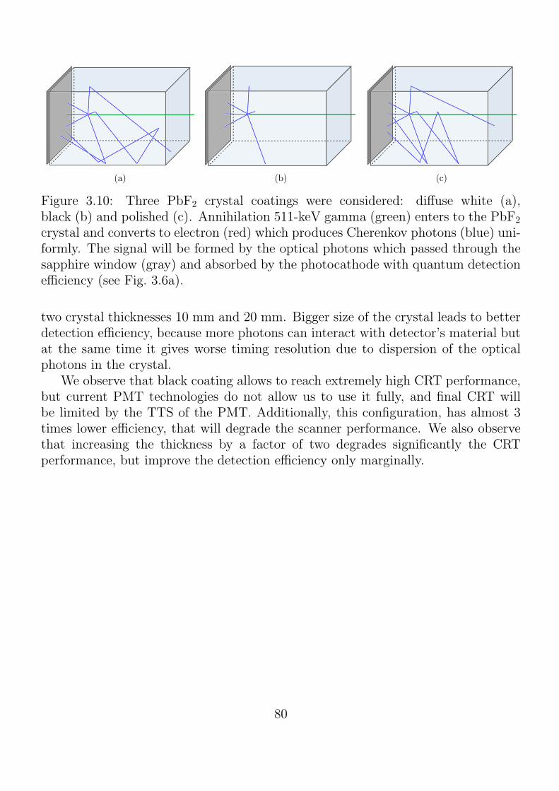
(a) (b) (c)

Figure 3.10: Three PbF2 crystal coatings were considered: diffuse white (a),black (b) and polished (c). Annihilation 511-keV gamma (green) enters to the PbF2

crystal and converts to electron (red) which produces Cherenkov photons (blue) uni-formly. The signal will be formed by the optical photons which passed through thesapphire window (gray) and absorbed by the photocathode with quantum detectionefficiency (see Fig. 3.6a).

two crystal thicknesses 10 mm and 20 mm. Bigger size of the crystal leads to betterdetection efficiency, because more photons can interact with detector’s material butat the same time it gives worse timing resolution due to dispersion of the opticalphotons in the crystal.

We observe that black coating allows to reach extremely high CRT performance,but current PMT technologies do not allow us to use it fully, and final CRT willbe limited by the TTS of the PMT. Additionally, this configuration, has almost 3times lower efficiency, that will degrade the scanner performance. We also observethat increasing the thickness by a factor of two degrades significantly the CRTperformance, but improve the detection efficiency only marginally.

80

t, ns∆ 1− 0.8− 0.6− 0.4− 0.2− 0 0.2 0.4 0.6 0.8 1

0

200

400

600

800

1000

1200

1400FWHM = 133 psFWTM = 600 ps

Efficiency = 33.1 %

(a)

t, ns∆ 1.5− 1− 0.5− 0 0.5 1 1.5

0

200

400

600

800

1000

1200

1400

FWHM = 170 psFWTM = 1077 ps

Efficiency = 34.0 %

(b)

t, ns∆ 0.3− 0.2− 0.1− 0 0.1 0.2 0.3

0

50

100

150

200

250

FWHM = 40 psFWTM = 110 ps

Efficiency = 12.0 %

(c)

t, ns∆ 0.3− 0.2− 0.1− 0 0.1 0.2 0.3

0

20

40

60

80

100

120FWHM = 48 psFWTM = 108 ps

Efficiency = 10.5 %

(d)

t, ns∆ 1.5− 1− 0.5− 0 0.5 1 1.5

0

200

400

600

800

1000

1200

1400

1600

1800FWHM = 150 psFWTM = 800 ps

Efficiency = 35.0 %

(e)

t, ns∆ 2− 1.5− 1− 0.5− 0 0.5 1 1.5 2

0

200

400

600

800

1000

1200

1400

1600

FWHM = 220 psFWTM = 1613 ps

Efficiency = 37.5 %

(f)

Figure 3.11: Simulating results of the CRT estimation with point-like radioactivesource at the center FOV and without TTS of the MCP-PMT for three differentcrystal coatings and two crystal thicknesses: (a) 10-mm thick and (b) 20-mm thickdiffuse white crystal, (c) 10-mm thick and (d) 20-mm thick black crystal, (e) 10-mmthick and (f) 20-mm thick polished lead fluoride crystal.

81

3.4 Simulated scanner geometry

In order to estimate the potential of the Cherenkov technology for the whole-bodyPET, we developed the simulation of the complete scanner (see Fig. 3.12a). In thefollowing section we will study different scanner configurations following the NEMAstandard [35], and will conclude on the potential of different configurations.

We choose to associated a single PbF2 crystal to each anode of the MCP-PMT.It results in the detection modules made with one PMT and 64 crystals with thesize 6.5 × 6.5 × 10 (20) mm3, glued together. We assume, that each individualcrystal is optically isolated from the neighbors and has the diffuse white surface asdescribed above.

(a) (b)

Figure 3.12: (a) Layout of the three rings whole-body Cherenkov TOF-PET scannerwith lead shielding (colored in red) has been used in the GATE simulation; (b)scheme of the PET detection unit, which consists of a block of 64, 8 × 8 × 1,individual PbF2 crystals attached to a single photomultiplier with the same anodestructure, 8 × 8.

We will compare the current simulation with the measurement of the non-TOFcommercially available scanner Discovery d-690 [21]. This is a three rings scannerwith the axial FOV of 157 mm. To have an equivalent solid angle we chose to simu-late the three rings scanner. It results in a axial FOV of 180 mm. We tested the tworing diameters 81 cm and 91 cm. We found that the optimal NECR characteristics

82

(described in the Section 4.2) are for the diameter 81 cm. Each ring consist of 43or 48 detection blocks 3.12b and for 81 cm and 91 cm diameters the total numberof PMT is 129 or 144 correspondingly. The total number of crystals is 8256 or9216. We also study the lead shielding option for protecting the scanner from theout-of-FOV gamma (see Fig. 2.4d). We found that a annulus-shape shielding withthe internal diameter of 70 cm, external diameter of 108 cm and thickness of 3 cmreduce the out-of-FOV contribution by a factor of 0.2.

83

Chapter 4

PET performance estimationaccording to the NEMA NU2-2007 Standard

4.1 CRT

Coincidence resolving time (CRT) is one of the main characteristics of the scanner.In the Section 3.3.3 we estimated CRT for three different crystal coatings with point-like radioactive source placed in the center of FOV. In this chapter we will discussonly about diffuse white crystal coating because it was chosen as an optimal.

For realistic CRT estimation we take into account the TTS of PMT of 80 ps.We used the polyethylene test phantom, the same as for the NECR calculation (seeSection 4.2.1). The linear radioactive source inserted in the phantom at the 45 mmdistance from the center FOV. We considered two crystal thicknesses 10 mm (seeFig. 4.1a) and 20 mm (see Fig. 4.1b) with molecular bonding optical interface oroptical gel (see Fig. 4.1c). As expected, the best CRTperformance is obtained forthe 10 mm crystal with molecular interface bonding.

Compare to our previous results (see Section 3.3.3) we observe a significantdegradation, more than expected, for the configuration with the crystal thickness20 mm. Most probably, this degradation could be explained by the fact that thephantom has rather large diameter of 20 mm. Such configuration will generate a lotof gamma with the large impact parameter (i.e. passing far from the center). In thecase of the thick crystal such, non-central, gamma are converted far from the PMTwindow, and the generated optical photons have trajectories with many reflection,due-to the directional character of the Cherenkov radiation. As it will be explainedlater in the Section 4.2, the obtained value of CRT will be used to account for thetime-of-flight potential in noise equivalent count rates calculation.

84

t, ns∆

1− 0.8− 0.6− 0.4− 0.2− 0 0.2 0.4 0.6 0.8 1

Co

incid

en

ce

s

0

1000

2000

3000

4000

5000

6000

7000

8000

9000FWHM = 180 ps

FWTM = 780 ps

(a)

t, ns∆

1− 0.8− 0.6− 0.4− 0.2− 0 0.2 0.4 0.6 0.8 1

Co

incid

en

ce

s

1000

2000

3000

4000

5000

6000

7000

8000

9000

FWHM = 380 ps

FWTM = 1440 ps

(b)

t, ns∆

1− 0.8− 0.6− 0.4− 0.2− 0 0.2 0.4 0.6 0.8 1

Co

incid

en

ce

s

0

200

400

600

800

1000

1200

1400

1600

1800

2000

2200

FWHM = 240 ps

FWTM = 940 ps

(c)

Figure 4.1: Realistic CRT estimation for configuration with molecular bonding and10-mm thick crystal (a) and 20-mm thick crystal (b) in comparison with CRT forconfiguration with optical gel and 10-mm thick crystal (c).

4.2 NECR

Noise equivalent count rates (NECR) is an ”effective” count rate, which allows tocompare the theoretical signal-to-noise ratios, achievable in images from differentscanner without image reconstruction. This parameter is a major arguing point forsome vendors determined partly by detector type, detector and scanner geometry,acquisition mode, and front-end electronics. Higher NECR value leads to betterimage quality. The procedure of the NECR measurement recommended in the stan-dard NEMA [35] is based on the work Strother et al [106] and can be defined by:

NECR =T 2

T + S + 2R, (4.1)

or

NECR =T 2

T + S +R, (4.2)

85

where T , S and R are the number of true, scatter and random coincidencesrespectively (see definition in section 2.4).

The choice of the 2R or 1R parameter depends on the method used for theestimation of random coincidence number. In our work we choose to compare thesimulated results with the measurement of the NECR for conventional PET scannerDiscovery-D690 described in the publication Bettinardi et al [21]. They emphasizedthe importance of presence of a 2R random coincidence term because it is assumedthat the randoms estimate is not smoothed. In order to compare equivalent numbersin the following estimations we used 2R definition for all calculations.

4.2.1 Phantom NEMA for NECR

The test phantom is shown in Fig. 4.2 is a circular cylinder composed of the polyethy-lene with density of 0.96 g/cm3, with an outside diameter of about 200 mm andwith an overall length of about 700 mm [35]. We implemented a 700 mm long,linear radioactive source at the distance of 45 mm from the center of the polyethy-lene cylinder with inside diameter of 3.2 mm and an outside diameter 4.8 mm. Wesimulated phantom activities from 10 to 55 kBq/cm3 (see Tab. 4.1).

In order to speed-up the simulation, we generated directly two back-to-back511 keV photons in each event, without simulating the radioactive decay and positronthermalization. The distribution of the two-photon vertex (corresponding to theelectron-positron annihilation) are chosen to be uniform inside a source and both,φ and θ, angular distributions are isotropic.

Activity kBq/cm3 Total Activity MBq10 219.815 329.720 439.625 549.530 659.440 879.250 1099.055 1208.9

Table 4.1: Activity of the linear radioactive source used for NECR estimation.

Algorithm of the NECR estimation proposed in the standard NEMA [35] imposesto use the sinogram-based procedure. In this procedure each prompt and randomsinogram i of each acquisition j is masked with a 12 cm region from the center of thephantom. All the pixels outside the masked region are set to zero. Each projectionof the prompt sinogram is shifted to align the pixel with the maximum value in the

86

Figure 4.2: The polyethylene test phantom for NECR estimation with linear sourceinsert (blue).

center of the sinogram. The total events number and random events number arecalculated as the sum of counts within the masked region. Random plus scatterevents were computed by estimating the events under a 40-mm-wide strip centeredon the peak and adding these events to counts outside this strip.

Figure 4.3: LORs selection for NECR estimation.

In this work we used the list-mode output from GATE, which include infor-mation about the origin of both detected photon and scattering history for them.In order to simplify the estimation we used the following approach based on thesimulation information stored in each coincidence. In this procedure we define thetrue coincidence as a coincidence where both photons are generated by the sameannihilation vertex. Scatter coincidence is a coincidence in which two photons aregenerated by the same vertex, but at least one photon undergo the Compton scat-

87

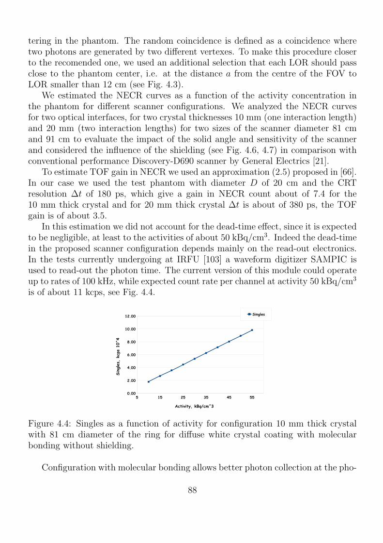
tering in the phantom. The random coincidence is defined as a coincidence wheretwo photons are generated by two different vertexes. To make this procedure closerto the recomended one, we used an additional selection that each LOR should passclose to the phantom center, i.e. at the distance a from the centre of the FOV toLOR smaller than 12 cm (see Fig. 4.3).

We estimated the NECR curves as a function of the activity concentration inthe phantom for different scanner configurations. We analyzed the NECR curvesfor two optical interfaces, for two crystal thicknesses 10 mm (one interaction length)and 20 mm (two interaction lengths) for two sizes of the scanner diameter 81 cmand 91 cm to evaluate the impact of the solid angle and sensitivity of the scannerand considered the influence of the shielding (see Fig. 4.6, 4.7) in comparison withconventional performance Discovery-D690 scanner by General Electrics [21].

To estimate TOF gain in NECR we used an approximation (2.5) proposed in [66].In our case we used the test phantom with diameter D of 20 cm and the CRTresolution ∆t of 180 ps, which give a gain in NECR count about of 7.4 for the10 mm thick crystal and for 20 mm thick crystal ∆t is about of 380 ps, the TOFgain is of about 3.5.

In this estimation we did not account for the dead-time effect, since it is expectedto be negligible, at least to the activities of about 50 kBq/cm3. Indeed the dead-timein the proposed scanner configuration depends mainly on the read-out electronics.In the tests currently undergoing at IRFU [103] a waveform digitizer SAMPIC isused to read-out the photon time. The current version of this module could operateup to rates of 100 kHz, while expected count rate per channel at activity 50 kBq/cm3

is of about 11 kcps, see Fig. 4.4.

Figure 4.4: Singles as a function of activity for configuration 10 mm thick crystalwith 81 cm diameter of the ring for diffuse white crystal coating with molecularbonding without shielding.

Configuration with molecular bonding allows better photon collection at the pho-

88

(a) (b)

Figure 4.5: Trues, scatters and randoms coincidence rates as a function of activityfor configuration 10 mm thick crystal with 81 cm diameter of the ring for diffusewhite crystal coating with molecular bonding (a) and with optical gel (b).

(a) (b)

Figure 4.6: NECR curves of the foreseen Cherenkov TOF-PET whole-body three-rings scanner based on 10-mm thick crystal with diffuse white crystal coating, 81 cmdetector’s ring diameter in comparison with conventional Discovery-D690 (magentacurve). (a) Comparison of two optical interfaces: molecular bonding (yellow curve)and with optical gel OCF452 (red curve) without TOF (continuous) and with TOF(dashed curves) with the same color of the lines respectively; (b) Influence of theshielding on NECR curves: continuous dark blue curve is NECR curve after imple-mentation the lead shielding in case without TOF and dashed curve is with TOF.

89

(a) (b)

Figure 4.7: NECR curves of the foreseen Cherenkov TOF-PET whole-body three-rings scanner based on 20 mm thick crystal with diffuse white coating in compari-son with conventional Discovery-D690 (magenta curve). (a) Comparison of NECRcurves for crystal thicknesses: 10 mm and 20 mm without TOF (dark blue and greencurves) and with TOF the same color of lines but dashed respectively; (b) Influenceof the scanner size on NECR curves: diameters 81 cm and 91 cm, crystal thickness20 mm.

tocathode. In case of the optical gel interface, optical photons with large impingingangle are lost due to the reflection at the border between MCP-PMT and gel. Thephotons with the wavelength smaller than 300 nm are absorbed by the optical gel.This two effects leads to smaller number of the collected photons and large CRT.We see that without TOF, the crystal with 20 mm thickness is slightly more optimaldue to the higher efficiency. When we take into account a TOF performance, thecrystal with 10 mm thickness became more optimal, because of the better CRT. Asshown at the Fig. 4.6b adding a lead shielding improve the NECR by about 20 %due to the better removal of the random coincidences.

The scanner diameter is also an important parameter to optimize. Larger diam-eter allows to reduce the parallax error and hence improve the spatial precision. Itis also improve the NECR values, for example for the scanner with diameter 91 cmincrease NECR by about 10 % compare to the diameter 81 cm, Fig. 4.7b. The draw-back of the higher diameter is a larger number of the detection module and hence ahigher price. For example, increasing the diameter from 81 to 90 cm increases therequired number of the photo-detectors from 43 to 48, i.e increase by 11 %. For thefollowing tests we retain a diameter of 81 cm as an optimal configuration for thescanner, with the NECR curves shown at Fig. 4.7a.

The coincidence polices available in GATE are described in the Section 2.4. Thepreliminary study of the coincidence policies with non-optimized scanner leads to the

90

# GATE Policy NameCoincidences Trues Randoms Scatters NECR

kcps kcps % kcps % kcps % kcps1 takeAllGoods 1791.630 417.304 23 1036.230 58 338.095 19 61.582 takeWinnerOfGoods 985.768 213.284 22 582.339 59 190.145 19 29.013 takeWinnerIfIsGood 826.185 175.845 21 491.480 59 158.860 19 23.474 takeWinnerIfAllAreGoods 516.313 101.071 20 314.535 61 100.707 20 12.305 keepIfOnlyOneGood 513.620 99.821 19 313.055 61 100.744 20 12.056 keepIfAnyIsGood 513.966 100.326 20 312.884 61 217.172 20 12.177 keepIfAllAreGoods 513.544 100.185 20 312.682 61 100.677 20 12.158 killAllIfMultipleGoods 515.014 100.453 20 313.841 61 100.720 20 12.179 killAll 514.238 100.155 19 313.633 61 100.450 20 12.12

Table 4.2: Comparison GATE coincidences policies for NECR estimation.

decision to use policy #2 takeWinnerOfGoods. We should note that the Cherenkovdetector in the current configuration does not allow to measure the energy, butthe signal charge measured by PMT represents the number of the detected opticalphotons. We redone the study of the coincidence policy using the optimized scannerconfiguration. The results of this test are shown in the Table 4.2 calculated for theactivity of 30 kBq/cm3. It was found that the most optimal policy is a policy #1takeAllGoods. Unfortunately, the time constrains and significant CPU necessaryfor the NECR calculation, does not allow us to recalculate the new NECR in timeto be included to this manuscript, but this recalculation are foreseen to be done forpublication.

4.3 Spatial Resolution

To estimate the spatial resolution of the scanner we follow the NEMA standard [35]recommendation and simulate six small point-like sources which are localized asfollowing:

In the axial direction, along planes (1) at the center of the axial FOV and (2)one-fourth of the axial FOV from the center of the FOV.

In the transverse direction the source was positioned (1) 1 cm vertically fromthe center (to represent the center of the FOV, but positioned to avoid any possibleinconsistent results at the very center of the FOV), (2) at x = 0 and y = 10 cm,and (3) at x = 10 cm and y = 0 (see Fig. 4.8).

The transverse FOV and image matrix size determine the pixel size in the trans-verse slice. In order to measure the width of the point spread function as accuratelyas can practically be achieved, its FWHM should span at least three pixels. We ex-pected FWHM is about of 5 mm. We chose to use the pixel size of 1 mm (it shouldbe no bigger than one-third of the expected FWHM in all three dimensions during

91

At 1 cm radius

Transverse RES =(

RESx(0; 1; center) +RESy(0; 1; center)+RESx(0; 1; 1/4FOV ) +RESy(0; 1; 1/4FOV )

)

/4

Axial RES =(

RESz(0; 1; center) +RESz(0; 1; 1/4FOV ))

/2

At 10 cm radius

Transverse radial RES =(

RESx(10; 0; center) +RESy(0; 10; center)+RESx(10; 0; 1/4FOV ) +RESy(0; 10; 1/4FOV )

)

/4,

Transverse tangential RES =(

RESy(10; 0; center) +RESx(0; 10; center)+RESy(10; 0; 1/4FOV ) +RESx(0; 10; 1/4FOV )

)

/4,

Axial resolution RES =(

RESz(10; 0; center) +RESz(0; 10; center)+RESz(10; 0; 1/4FOV ) +RESz(0; 10; 1/4FOV )

)

/4,

Table 4.3: According to NEMA 2-2007 standard [35], this is formulas for spatialresolution estimation, where RESi is a measurement of the size of the reconstructedimage FWHM of a point source i, center is a point with z coordinate equals 0 and1/4FOV for foreseen Cherenkov PET scanner is 4.5 cm.

reconstruction). Each FWHM was determined by linear interpolation between ad-jacent pixels at half the maximum value of the response function. The maximumvalue was determined by a parabolic fit using the peak point and its two nearestneighboring points respectively (see Fig. 4.9-Fig. 4.14).

We used following formulas to evaluate our results (see Tab. 4.3) of the axial,radial and tangential resolutions (FWHM) for each radius (center FOV and 10 cm),averaged over both axial positions. The acollinearity of 0.5 of two photon was takeninto account.

92

Figure 4.8: Positioning of the radioactive sources for spatial resolution estimation ofthe foreseen Cherenkov PET scanner with axial FOV 18 cm. The sources were fixedparallel to the long axis of the tomograph and located at 6 points as follows: 1: (0;1; 0) is green; 2:(0; 10; 0) is blue; 3: (10; 0; 0) is yellow; 4: (0; 1; -4.5) is magenta;5: (0; 10; -4.5) is gray; 6: (10; 0; -4.5) is cyan. All coordinates of the radioactivesources are given in cm.

4− 2− 0 2 4x, mm

0

0.0005

0.001

0.0015

0.002

0.0025

0.003

0.0035

0.004

0.0045

Valu

e

FWHM = 5.1 mm

(a)

4− 2− 0 2 4x, mm

0.0005

0.001

0.0015

0.002

0.0025

0.003

0.0035

0.004

0.0045

0.005

Valu

e

FWHM = 5.4 mm

(b)

4− 2− 0 2 4x, mm

0

0.0005

0.001

0.0015

0.002

0.0025

0.003

0.0035

0.004

Valu

e

FWHM = 5.6 mm

(c)

Figure 4.9: (a) X-profile, (b) Y-profile and (c) Z-ptofile for point-like source atposition (0;1;0).

93

4− 2− 0 2 4x, mm

0.0005

0.001

0.0015

0.002

0.0025

0.003

0.0035

0.004

0.0045

Valu

e

FWHM = 5.6 mm

(a)

4− 2− 0 2 4x, mm

0.001

0.002

0.003

0.004

0.005

0.006

Valu

e

FWHM = 4.6 mm

(b)

4− 2− 0 2 4x, mm

0

0.0005

0.001

0.0015

0.002

0.0025

0.003

0.0035

0.004

0.0045

Valu

e

FWHM = 5.2 mm

(c)

Figure 4.10: (a) X-profile, (b) Y-profile and (c) Z-ptofile for point-like source atposition (0;10;0).

4− 2− 0 2 4x, mm

0.001

0.0015

0.002

0.0025

0.003

0.0035

0.004

0.0045

0.005

Valu

e

FWHM = 5.7 mm

(a)

4− 2− 0 2 4x, mm

0.0005

0.001

0.0015

0.002

0.0025

0.003

0.0035

0.004

0.0045

0.005

Valu

e

FWHM = 6.3 mm

(b)

4− 2− 0 2 4x, mm

0

0.001

0.002

0.003

0.004

0.005

0.006

Valu

e

FWHM = 4.2 mm

(c)

Figure 4.11: (a) X-profile, (b) Y-profile and (c) Z-ptofile for point-like source atposition (10;0;0).

4− 2− 0 2 4x, mm

0.0005

0.001

0.0015

0.002

0.0025

0.003

0.0035

0.004

0.0045

Valu

e

FWHM = 5.1 mm

(a)

4− 2− 0 2 4x, mm

0.001

0.0015

0.002

0.0025

0.003

0.0035

0.004

0.0045

0.005

Valu

e

FWHM = 6.5 mm

(b)

4− 2− 0 2 4x, mm

0

0.0005

0.001

0.0015

0.002

0.0025

0.003

0.0035

0.004

0.0045

Valu

e

FWHM = 5.2 mm

(c)

Figure 4.12: (a) X-profile, (b) Y-profile and (c) Z-ptofile for point-like source atposition (0;1;-4.5).

94

4− 2− 0 2 4x, mm

0.001

0.002

0.003

0.004

0.005

0.006

0.007

0.008

Valu

e

FWHM = 5 mm

(a)

4− 2− 0 2 4x, mm

0.001

0.002

0.003

0.004

0.005

0.006

0.007

0.008

0.009

Valu

eFWHM = 5.6 mm

(b)

4− 2− 0 2 4x, mm

0

0.001

0.002

0.003

0.004

0.005

0.006

0.007

Valu

e

FWHM = 5.3 mm

(c)

Figure 4.13: (a) X-profile, (b) Y-profile and (c) Z-ptofile for point-like source atposition (0;10;-4.5).

4− 2− 0 2 4x, mm

0.001

0.002

0.003

0.004

0.005

0.006

Valu

e

FWHM = 4.4 mm

(a)

4− 2− 0 2 4x, mm

0.001

0.002

0.003

0.004

0.005

0.006

Valu

e

FWHM = 5.2 mm

(b)

4− 2− 0 2 4x, mm

0

0.001

0.002

0.003

0.004

0.005

Valu

e

FWHM = 4.7 mm

(c)

Figure 4.14: (a) X-profile, (b) Y-profile and (c) Z-ptofile for point-like source atposition (10;0;-4.5).

95

As was expected, spatial resolution degrades from the center FOV to a peripheryfrom 4.5 to 6.5 mm on each axis respectively and comparable with spatial resolutionof the conventional scanner Discovery D-690 [21]. The estimated uncertainty is abouthalf of the voxel size, i.e.± 0.25 mm. The configuration with molecular bonding hasspatial resolution comparable with optical gel configuration and slightly better thanspatial resolution of the conventional scanners. This explains by the fact that in ourconfiguration the crystal size and FOV are similar to the conventional scanner,butwe study the PbF2 crystal with small thickness, 10 mm, and hence smaller parallaxerror due to the uncertainty on DOI. In addition, PbF2 crystal has a two times higherphoto-electric fraction than LYSO crystals and, consequently, the number of eventswith two conversion points (one Compton scattering and one photo-ionization) issmaller. Such events with two conversion points will have worse spatial resolution,when these conversions happen in the different crystals.

4.4 Image quality and Contrast Recovery Coeffi-cients (CRC)

The prediction of the image quality of the foreseen Cherenkov PET scanner is non-trivial procedure due to the complex interplay of many different aspects of the systemperformance.

Standard NEMA proposes to compare the image quality of different systemsusing a standardized image quality phantom that simulates a clinical imaging con-dition. The proposed phantom with non-uniform attenuation (see Fig. 4.15) is filledwith background activity. It contains four ”hot” spheres, e.g. spheres with activitysignificantly higher than the background one, and two ”cold” spheres, e.g. sphereswith no activity. Six spheres have different diameters and are used to estimate thecontrast recovery after the image reconstruction, while background region is used toestimate the background variability.

The concentration of the background activity in the phantom is 5.3 kBq/cm3,which corresponds to typical injected dose for whole-body studies. The total volumeof the body phantom was divided on 4 parts (I, II, III and IV). For each partthe partial volume was calculated with subtraction of the volumes of all inserts:VI = 6809.44[cm3], VII = VIII = 996[cm3], VIV = 2289.84[cm3].

Voxel size is 2.5 mm and reconstructed image is 128 × 128 pixels. We did notreconstruct whole length of the phantom in order to reduce the CPU time neededfor the reconstruction, but only region with hot and cold spheres were reconstructedplus ± 4.25 cm from the central slice (#18), 35 slices in total.

A transverse image centered on the cold and hot spheres is used in the analysis,which was provided in the FIJI (the latest version of ImageJ) analysis software [107].

96

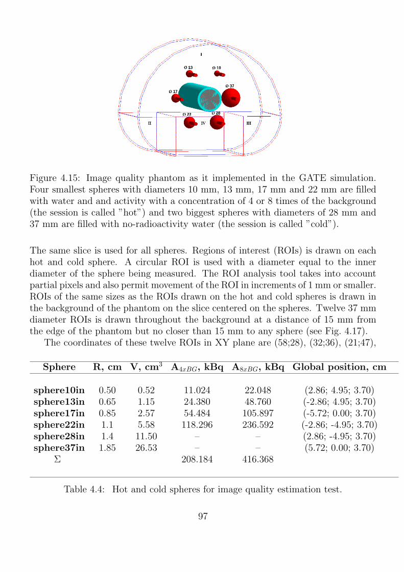
Figure 4.15: Image quality phantom as it implemented in the GATE simulation.Four smallest spheres with diameters 10 mm, 13 mm, 17 mm and 22 mm are filledwith water and and activity with a concentration of 4 or 8 times of the background(the session is called ”hot”) and two biggest spheres with diameters of 28 mm and37 mm are filled with no-radioactivity water (the session is called ”cold”).

The same slice is used for all spheres. Regions of interest (ROIs) is drawn on eachhot and cold sphere. A circular ROI is used with a diameter equal to the innerdiameter of the sphere being measured. The ROI analysis tool takes into accountpartial pixels and also permit movement of the ROI in increments of 1 mm or smaller.ROIs of the same sizes as the ROIs drawn on the hot and cold spheres is drawn inthe background of the phantom on the slice centered on the spheres. Twelve 37 mmdiameter ROIs is drawn throughout the background at a distance of 15 mm fromthe edge of the phantom but no closer than 15 mm to any sphere (see Fig. 4.17).

The coordinates of these twelve ROIs in XY plane are (58;28), (32;36), (21;47),

Sphere R, cm V, cm3 A4xBG, kBq A8xBG, kBq Global position, cm

sphere10in 0.50 0.52 11.024 22.048 (2.86; 4.95; 3.70)sphere13in 0.65 1.15 24.380 48.760 (-2.86; 4.95; 3.70)sphere17in 0.85 2.57 54.484 105.897 (-5.72; 0.00; 3.70)sphere22in 1.1 5.58 118.296 236.592 (-2.86; -4.95; 3.70)sphere28in 1.4 11.50 – – (2.86; -4.95; 3.70)sphere37in 1.85 26.53 – – (5.72; 0.00; 3.70)

Σ 208.184 416.368

Table 4.4: Hot and cold spheres for image quality estimation test.

97

(12;60), (14;75), (25;86), (39;91), (57;91), (83;89), (97;84), (105;70) and (84;35) inimage coordinate (see Fig. 4.16).

Figure 4.16: Image coordinates in pixels.

Figure 4.17: For background variability estimation twelve regions of interest (ROIs)were chosen to +/-1 cm and +/-2 cm on either side of the central slice with diametersare close as possible to the physical inner diameters of the spheres from 10 mm to37 mm. ROIs of the smaller sizes (10, 13, 17, 22, and 28 mm) are drawn concentricto the 37-mm background ROIs.

In total of 60 background ROIs of each size, 12 ROIs on each of 5 slices wereconsidered (slices 10th, 14th, 18th, 22nd and 26th). The locations of all ROIs werefixed between successive measurements (e.g., replicate scans). The average numberof counts in each background ROI was recorded. The percent contrast QH,j for each

98

hot sphere j is calculated by:

QH,j =

CH,j

CB,j− 1

aHaB

− 1· 100 %, (4.3)

where CH,j is the average number of counts in the ROI for sphere j; CB,j isthe average number of the background ROI counts for sphere j; aH is the activ-ity concentration in the hot spheres, and aB is the activity concentration in thebackground.

The percent contrast QC,j for each cold sphere j is calculated by:

QC,j =

(

1−CC,j

CB,j

)

· 100 %, (4.4)

where CC,j is the average number of counts in the ROI for sphere j; CB,j is theaverage number of the 60 background ROI counts for sphere j.

The percent background variability Nj for sphere j is calculated as:

Nj =σjCB,j

· 100 %, (4.5)

where σj is the standard deviation of the background ROI counts for sphere j,calculated as:

σj =

√

√

√

√

√

k∑

k=1

(CB,j,k − CB,j)2

(k − 1), k = 60. (4.6)

The wall thickness of the spheres is of 1 mm. Phantom material describedin NEMA is polymethylmethacrylate, for modeling we used material plastic withdensity 1.18 g/cm3, molecular formula C5H8O2.

Estimated contrast recovery coefficients Qj [%] and background variability Nj

[%] are shown in Tab. 4.5 – Tab. 4.8.In particular, Tab. 4.5 represents CRC in case any attenuation corrections (No-

Corr) and with attenuation correction procedure (WithCorr) for configurations with-out TOF (NoTOF) and with TOF capability (TOF) for 1 hour scanning, (seeFig. 2.10). Attenuation correction in the phantom improves the ratio signal-to-noiseat least of 2.5 times.

For more realistic estimation of the CRC we decreased the scanning time to15 min and investigated the impact of the number of iterations and subsets on thequality of the PET image, Tab 4.6.

99

Sphere, mm Parameter, %NoTOF TOF 140 ps

NoCorr WithCorr NoCorr WithCorr

10QH,j -0.9 7.3 3.7 11.5Nj 15.2 6.2 7.8 5.2

13QH,j 0.9 8.8 6.9 16.3Nj 13.2 5.2 7.4 4.5

17QH,j 3.3 17.1 12.7 25.3Nj 13.1 4.6 7.3 4.1

22QH,j 6.2 21.4 18.0 31.0Nj 13.2 4.2 7.3 3.8

28QC,j 52.3 4.2 41.1 25.1Nj 13.2 4.1 7.3 3.7

37QC,j 53.8 5.5 44.1 28.6Nj 17.3 4.7 8.6 4.2

Table 4.5: Contrast recovery factor Qj [%] and background variability Nj [%] with-out attenuation correction (NoCorr) and with attenuation correction (WithCorr) forcases without TOF (NoTOF) and with TOF capability (TOF <CRT> [ps]), timeof scanning is 1 hour (see Fig. 2.10).

Sphere5 subsets, 1st iteration no subsets, 5th iteration no subsets, 10th iteration

NoTOF (0.0022) TOF 250 ps NoTOF (0.0016) TOF 250 ps TOF 250 psQj Nj Qj Nj Qj Nj Qj Nj Qj Nj

10 2.9 5.7 4.1 9.2 2.9 5.8 4.3 9.3 5.6 (+23%) 14.2 (+35%)13 3.1 5.3 6.8 8.5 3.1 5.3 6.7 8.5 12.6 (+47%) 9.5 (+11%)17 5.2 5.2 11.2 7.9 5.1 5.2 11.1 7.9 12.7 (+13%) 11.4 (+31%)22 8.1 4.9 14.7 6.7 8.0 4.9 14.6 6.7 16.7 (+13%) 9.1 (+26%)28 3.1 4.6 34.6 6.0 3.4 4.6 34.6 6.0 43.4 (+20%) 8.0 (+25%)37 -1.4 5.5 35.6 5.0 -1.4 5.5 35.7 5.1 40.0 (+11%) 6.0 (+15%)

+21% +24%

Table 4.6: The contrast recovery factor Qj [%] and background variability Nj [%]with attenuation correction in the phantom for scanning time 15 min and lowerinitial contrast (4xBG) in case of variable number of iterations and subsets forMLEM image reconstruction algorithm (see Fig. 4.18)

.

100

(a) (b)

(c) (d)

Figure 4.18: Reconstructed images of the Body Phantom NEMA, time of the scan-ning 900 s associated with Tab. 4.6 in case: (a) without TOF, with attenuationcorrection, 1st iteration with 5 subsets; (b) resolving time TOF 250 ps with atten-uation correction, 1st iteration with 5 subsets; (c) resolving time TOF 250 ps, withattenuation correction, 5th iteration with 1 subset; 4) resolving time TOF 250 ps,with attenuation correction, 10th with 1 subset.

101

As was discussed in the Section 2.6.4, applying of the Cherenkov photons forcreation a PET scanner requires another development of the random correction,which goes beyond the scope of the current study. In order to mitigate the absenceof the scatter and random corrections, we reconstructed the PET image by takinginto account only true coincidences. Indeed, the reconstruction of such image couldbe viewed as a reconstruction of all coincidences when perfect random and scattercorrections are applied. Of course, in the real life those corrections are never per-fect, but we can reasonably expect that the result of the image reconstruction withrandom and scatter corrections will be located somewhere between two boundarycases: (1) image produced by all coincidences without any corrections and (2) theimage created by only true coincidences. Therefore, Table 4.8 represents the resultsof the estimation of the contrast recovery coefficients and background variability incase taking into account only true coincidences for two activity concentrations of thehot spheres, 4 and 8 times over the background radioactivity (4xBG and 8xBG). Forthis estimation we used MLEM reconstruction algorithm and results of the 5th and10th iterations are shown. As was expected, the increasing of quantity of iterationincreases the CRC, but at the cost of the larger background fluctuations.

Furthermore, we studied the influence of the reconstruction parameters suchas number of iterations and subsets on the image quality. For example, in case theOSEM reconstruction with 5 subsets, see Fig. 4.20. As once can see in Fig. 4.20a, 4.20c,increasing in CRC always corresponds to the increasing in the background fluctu-ation. In order, to determine the optimal point, we calculated the signal-to-noiseratio (SNR) defined as:

SNR =QH,j −QB,j

σj, (4.7)

where QH,j is average counts in the ROI for sphere j, QB,j is average countsin a ROI for background, σj is standard deviation of the background ROI counts,corresponding to noise in the image. The best CRC is found to be for the firstiteration in the case of the 5 subsets.

We also compare the obtained contrast recovery with the conventional hybridscanner Biograph mMR by Siemens Healthcare [108], see Tab 4.7. As one can seethe obtained contrast recovery are smaller than for the conventional scanner, butobtained value are still reasonable to identify all hot sphere at the high contrast(8xBG) and identify the two largest at the low contrast (4xBG).

The influence of the varying reconstruction parameters on image quality is demon-strated for the four smallest spheres in Fig. 4.20. It can be determined that contrastrecovery coefficients increase with an increasing number of the iterations at the costof higher background variability.

102

Sphere, mmPECHE scanner Biograph mMR by Siemens

Qj, [%] 4xBG Qj, [%] 8xBG Qj, [%], 4xBG (MRI) Qj, [%] 4xBG, (CT)10 5.0 20.6 16.8 30.513 11.0 27.0 31.7 50.517 16.8 42.6 52.7 72.922 21.1 51.3 64.8 74.528 61.9 63.1 68.8 56.637 69.3 67.6 76.1 64.8

Table 4.7: Contrast recovery factor Qj cases TOF 180 ps, time of scanning 15 min,initial contrast is 4 and 8 (see Fig. 4.19) in case only true reconstructed coincidencesand comparison with conventional scanners MR-based 3.0 Tesla PET/MR hybridsystem (Biograph mMR, Siemens Healthcare) and CT-based [108].

SphereActivity 4xBG Activity 8xBGit5 it10 it5 it10

Qj Nj Qj Nj Qj Nj Qj Nj

10 4.2 10.4 6.1 17.9 19.1 5.1 27.3 20.113 9.2 8.6 14.2 14.1 25.5 4.0 36.6 15.317 16.1 6.8 19.0 10.7 42.3 3.0 51.4 10.822 21.4 5.3 24.8 8.0 53.4 5.1 59.6 7.328 61.7 4.7 70.6 7.2 62.5 4.7 70.4 7.037 70.5 3.7 78.9 5.1 68.6 4.5 75.8 6.0

Table 4.8: Contrast recovery factorQj [%] and background variability Nj [%] of theimage containing only true coincidence. Scan time 15 min, attenuation correction isincluded. Use MLEM reconstruction (no subsets), it5 corresponds to 5th iteration,it10 corresponds to 10th iteration.

103

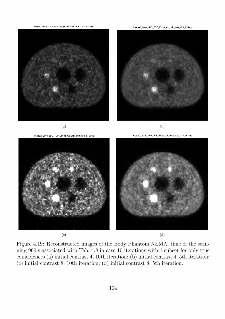
(a) (b)

(c) (d)

Figure 4.19: Reconstructed images of the Body Phantom NEMA, time of the scan-ning 900 s associated with Tab. 4.8 in case 10 iterations with 1 subset for only truecoincidences (a) initial contrast 4, 10th iteration; (b) initial contrast 4, 5th iteration;(c) initial contrast 8, 10th iteration; (d) initial contrast 8, 5th iteration.

104

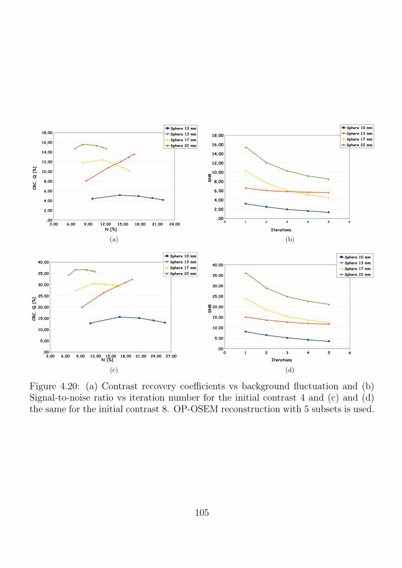
(a) (b)

(c) (d)

Figure 4.20: (a) Contrast recovery coefficients vs background fluctuation and (b)Signal-to-noise ratio vs iteration number for the initial contrast 4 and (c) and (d)the same for the initial contrast 8. OP-OSEM reconstruction with 5 subsets is used.

105

Conclusion

The time-of-flight technology has a very high potential to improve positron emissiontomography. It increases the signal-to-noise ratio of the reconstructed images andprovides the possibility to further improvement of already very high PET scannerssensitivity (the pico-molar level). If the present state-of-the-art coincidence timeresolution of about 325 ps could be improved, it allows to get a significant reductionof the dose injected to a patient, and consequently, the possibility to extend the useof the PET scans to new categories of the patients.

The study presented in this manuscript demonstrated that the Cherenkov de-tection technology could reach the equivalent or even better performance than theconventional technology based on the scintillation crystals. In particular, we esti-mated that the TOF NECR values of the foreseen Cherenkov scanner are comparableor even better than ones reached by the commercial machine. The image qualityparameters, i.e., contrast recovery versus background fluctuation are slightly worsethan the chosen example of the commercial scanner, but this comparison still re-quires further optimization of the reconstruction parameters.

In the same time, the results obtained should be taken with caution. It is wellknown, that simulation is more often optimistic compare to the real installations. Inparticular, in our study we should underline the following ”delicate” points. First ofall, the current simulation of the PMT time response do not take into account anypossible tails in the TTS distribution. As was discovered lately, the hardware testsat the IRFU [109] show that such tail exists and could degrade the detector timeresponse. Secondarily, that this simulation assumes the molecular bonding betweenPMT window and crystal [88]. As was shown in the Section 4.2, such configuration istwo times more efficient than the conventional optical interface using optical gel. Inthe same time, such configuration is technically difficult to realize. Indeed, the mainprinciple of the molecular bonding consists of bringing in contact the PMT sapphirewindow and PbF2 crystal, without using any additional material (e.g. optical gel).Such an operation requires surfaces polished to the level of roughness of 1 nm orbetter and planarity of these surfaces less than 1 µm. In addition, these surfaces mustbe also free from the dust particles and contamination, especially hydrocarbon films.This procedure was judged too difficult in realization and application on the PMTwindow, so we consider an another idea: direct deposition of the photocathode layeron the crystal surface and, thus, totally eliminate the total reflection between thephotocathode and the crystal. This idea will be studied in the ClearMind project,which has similar performances concerning the Cherenkov radiation detection asones was obtained in the current work.

Unfortunately, the lead fluoride is a fragile material. Moreover, when PbF2 crys-tal is heated to the temperatures necessary for the evaporation of the photocathode

106

layer, it degases the lead compounds, mainly PbF, toxic for the photocathode de-position. To avoid these problems, the use of the lead tungstate (PbWO4) crystalis proposed. This crystal has a high density (8.8 g/cm3) and a high atomic number(Z = 188). It degases considerably less than PbF2 and produces almost the samenumber of the Cherenkov photons. Additionally, it generates a small amount of thescintillation photons, which are relatively fast. This additional light increases thenumber of the detected optical photons and correspondingly the time resolution, andit also makes possible to measure the deposited energy and reconstruct the positionof the gamma interactions using a monolithic crystal. As a continuation of this workit is planned to adjust the simulation for use of monolithic lead tungstate crystalsand study the performances of the foreseen whole-body TOF PET scanner.

In this study we demonstrated that the relatively low detection efficiency of theCherenkov crystals is compensated by the TOF gain due to the high CRT resolution.In the same time, current resolution is limited by the TTS of the existing photo-multipliers. Even if the current performance of the Cherenkov scanner does not havesufficient motivation without additional developments, we expect that a continuousimprovement of the photo-detection technologies and, in particular time resolution,this approach becomes more interesting either by use of the pure Cherenkov ra-diators, or by use of the scintillation crystals with a significant production of theCherenkov light.

107

Acknowledgements

First of all, we acknowledge the financial support by the LabEx P2IO R&D projectof the region Ile-de-France, the IDI 2015 project funded by the IDEX Paris-Saclay,ANR-11-IDEX-0003-02, PhD financial support by the French embassy in Ukraine,Programme Transversal Technologies pour la Sante of the CEA, DRI UniversityParis-Saclay and Taras Shevchenko National University of Kyiv. This work is con-ducted within the scope of the IDEATE International Associated Laboratory.

In addition, I would like to thank my supervisor Viatcheslav Sharyy and co-supervisor Igor Kadenko for their participation and paying continuous attention tomy scientific and non-scientific problems. I gratefully acknowledge the best groupCaLIPSO at the IRFU for their patience and help in overcoming numerous obstaclesI have been facing through my PhD research. Many thanks to the IRFU for itsworking and friendly atmosphere.

I am very grateful to Achille Stocchi, Gerard Montarou, Klaus Peter Schafers andOleg Bezshyyko for accepting to be part of the jury and their edits and correctionsfor this thesis.

Larisa Golinka-Bezshyyko deserves a lot of gratefulness for her advice.I would like to thank all my friends for staying by my side and sharing various

moments of my life.Last but not the least, I would like to thank my family: my lovely and patient

husband, my wonderful daughter and my super parents for incredible supporting methroughout writing this thesis and my existence in general.

108

Bibliography

[1] R. Bar-Shalomab, A. Y. Valdivia, and M. D. Blaufox, “PET Imaging in On-cology,” Sem Nucl Med, vol. 30, pp. 150–185, 2000.

[2] E. de Groot et al., “Optimized dose regimen for whole-body FDG-PET imag-ing,” EJNMMI Research, vol. 3, no. 1, p. 63, 2013.

[3] B. Huang, M. W.-M. Law, and P.-L. Khong, “Whole-Body PET/CT Scanning:Estimation of Radiation Dose and Cancer Risk,” Radiology, vol. 251, no. 1,pp. 166–174, 2009, pMID: 19251940.

[4] R. Campagnolo, P. Garderet, and J. Vacher, “Tomographie par emetteurspositrons avec mesure de temps de vol,” In Proc. Commun. au Colloque Na-tional sur le Traitement du Signal, Nice, France, May 1979.

[5] T. Tomitani, “Image Reconstruction and Noise Evaluation in Photon Time-of-Flight Assisted Positron Emission Tomography,” IEEE Trans Nucl Sci, vol. 28,no. 6, pp. 4581–4589, 1981.

[6] Ter-Pogossian et al., “Photon Time-of-flight-assisted Positron Emission To-mography,” J Comp As Tom, vol. 5, pp. 227–239, April 1981.

[7] Ter-Pogossian, et al., “Super PETT I: A Positron Emission Tomograph Utiliz-ing Photon Time-of-Flight Information,” IEEE Trans Med Imag, vol. 1, no. 3,pp. 179–187, Nov 1982.

[8] M. Yamamoto, D. Ficke, and M. Ter-Pogossian, “Experimental Assessmentof the Gain Achieved by the Utilization of Time-of-Flight Information in aPositron Emission Tomograph ”(Super PETT I)”,” IEEE Trans Med Imag,vol. 1, no. 3, pp. 187–192, Nov 1982.

[9] T. F. Budinger, “Time-of-Flight Positron Emission Tomography: Status Rel-ative to Conventional PET,” J Nucl Med, vol. 24, no. 1, p. 73, 1983.

109

[10] A. Mallon and P. Grangeat, “Three-dimensional PET Reconstruction WithTime-of-flight Measurement,” Phys Med Biol, vol. 37, no. 3, pp. 717–729,1992.

[11] Vereos Digital PET-CT, Philips U.S.A.

[12] M. Berger et al., “NIST Standard Reference Database 8 (XGAM),”https://www.nist.gov/pml/xcom-photon-cross-sections-database.

[13] S. Korpar et al., “Study of TOF PET Using Cherenkov Light,” Nucl InstrumMeth A, vol. 654, no. 1, pp. 532–538, 2011.

[14] S. Korpar et al., “Study of TOF PET Using Cherenkov Light,” Physics Pro-cedia, vol. 37, pp. 1531–1536, 2012, Proceedings of the 2nd International Con-ference on Technology and Instrumentation in Particle Physics (TIPP 2011).

[15] S. Korpar et al., “Study of a Cherenkov TOF-PET Module,” Nucl InstrumMethods Phys Res, vol. 732, pp. 595–598, 2013, Vienna Conference on Instru-mentation 2013.

[16] S. Ziegler, “Positron Emission Tomography: Principles, Technology, and Re-cent Developments,” Nucl Phys A, vol. 752, pp. 679c–687c, 2005.

[17] D. L. Miller and D. Schauer, “The ALARA Principle in Medical Imaging,”AAPM Newsletter, vol. 40, no. 1, pp. 38–40, 2015.

[18] M. Larobina, A. Brunetti, and M. Salvatore, “Small animal PET: a review ofcommercially available imaging systems,” Curr Med Imag Rev, vol. 2, no. 2,May 2006.

[19] H. W. A. M. de Jong et al., “Performance evaluation of the ECAT HRRT: anLSO-LYSO double layer high resolution, high sensitivity scanner,” Phys MedBiol, vol. 52, no. 5, p. 1505, February 2007.

[20] C. Weirich et al., “Simultaneous PET and MR Imaging with a Newly Devel-oped 3TMR-BrainPET Scanner,” CEUR Workshop Proceedings, pp. 201–205,2010.

[21] V. Bettinardi et al., “Physical Performance of the New Hybrid PET/CTDiscovery-690,” Med Phys, vol. 38, no. 10, pp. 5394–5411, 2011.

[22] IAEA, “Cyclotron Produced Radionuclides: Principles and Practice,” Techni-cal Reports Series No. 465, 2008.

110

[23] G. Saha, Fundamentals of nuclear pharmacy, 5th ed. Springer, New York,2004.

[24] G. Saha, W. MacIntyre, and R. Go, “Cyclotrons and positron emission tomog-raphy radiopharmaceuticals for clinical imaging,” Semin Nucl Med, vol. 22, pp.150–161, 1992.

[25] D. L. Bailey et al., Positron Emission Tomography Basic Sciences. Springer,London, 2005.

[26] B. Bendriem and D. Townsend, The Theory and Practice of 3D PET. KluwerAcademic Publishers, 1998.

[27] O. Klein and Y. Nishina, “Uber die Streuung von Strahlung durch freie Elek-tronen nach der neuen relativistischen Quantendynamik von Dirac,” Z Physik,vol. 52, pp. 853–868, 1928.

[28] J. H. Hubbell, “Review of photon interaction cross section data in the medicaland biological context,” Phys Med Biol, vol. 44, pp. R1–R22, 1999.

[29] E. Hecht, Optics, 5th ed. Pearson Education Limited, England, 2017.

[30] GEANT4 Collaboration, Geant4 User’s Guide for Application Developers, 6Dec 2013, version: geant4 10.0.

[31] A. Levin and C. Moisan, “A More Physical Approach to Model the SurfaceTreatment of Scintillation Counters and its Implementation into DETECT,”TRIUMF Preprint TRI-PP-96-64, 1996.

[32] P. Cerenkov, “Visible Radiation Produced by Electrons Moving in a Mediumwith Velocities Exceeding that of Light,” Phys Rev, vol. 52, p. 378, 1937.

[33] V. Jelle, “Cerenkov Radiation and Its Applications,” Br J Appl Phys, vol. 6,pp. 227–232, 1955.

[34] G. Collins and V. Reiling, “Cerenkov Radiation,” Phys Rev, vol. 54, pp. 499–503, 1938.

[35] National Electrical Manufacturers Association, “Performance Measurementsof Positron Emission Tomographs,” NEMA NU 2-2007, 2007.

[36] T. F. Budinger, “PET instrumentation: what are the limits?” Sem Nucl Med,vol. 28, pp. 247–267, 1998.

[37] https://explorer.ucdavis.edu/about explorer.

111

[38] G. Bolard et al., “Performance comparison of two commercial BGO-basedPET/CT scanners using NEMA NU 2-2001,” Med Phys, vol. 34, pp. 2708–2717, 2007.

[39] C. Melcher and J. Schweitzer, “Cerium-doped lutetium oxyorthosilicate: afast, efficient new scintillator,” IEEE Trans Nucl Sci, vol. 4, pp. 502–505,1992.

[40] Y. Hirano, K. Koshino, and H. Iida, “Influences of 3d PET scanner componentson increased scatter evaluated by a monte carlo simulation,” Phys Med Biol,vol. 62, no. 10, pp. 4017–4030, apr 2017.

[41] M. Gaens et al., “GPU-accelerated Monte Carlo based scatter correction inbrain PET/MR,” EJNMMI Phys, vol. 1, no. 1, p. A32, Jul 2014.

[42] C. H. Holdsworth et al., “Evaluation of a Monte Carlo scatter correction inclinical 3D PET,” 2003 IEEE Nucl Sci Symposium. Conference Record (IEEECat. No.03CH37515), vol. 4, pp. 2540–2544, Oct 2003.

[43] D. Bailey, T. Jones, and T. Spinks, “A Method for Measuring the AbsoluteSensitivity of Positron Emission Tomographic Scanners,” Eur J Nucl Med,vol. 18, pp. 374–379, 1991.

[44] G. Saha, Basics of PET Imaging Physics, Chemistry, and Regulations, 2nd ed.Springer, London, 2010.

[45] A. Braem et al., “Feasibility of a novel design of a high resolution parallax-freecompton enhanced pet scanner dedicated to brain research,” Phys Med Biol,vol. 49, pp. 1–16, 2004.

[46] G. Knoll, Radiation detection and measurement, 2nd ed. John Wiley & Sons,1989.

[47] D. Yvon et al., “CaLIPSO: A novel detector concept for positron annihilationdetection,” in Proc. 3rd Int Advancements in Nuclear Instrumentation Mea-surement Methods and their Applications (ANIMMA) Conf, Jun. 2013, pp.1–9.

[48] D. Townsend et al., “High-density avalanche chamber (HIDAC) positron cam-era,” J Nucl Med, vol. 28, pp. 1554–1562, 1987.

[49] A. Jeavons, R. Chandler, and C.A.R. Dettmar, “A 3D HIDAC-PET camerawith sub-millimetre resolution for imaging small animals,” IEEE Trans NuclSci, vol. 46, pp. 468–473, 1999.

112

[50] K. Bolwin et al., “Development of a clear sub-millimeter small animal PETscanner by reducing the influence of the non-collinearity effect,” Journal ofInstrumentation, vol. 12, no. 03, p. C03006, 2017.

[51] D. L. Thorek et al., “Cerenkov imaging - a new modality for molecular imag-ing,” Am J Nucl Med Mol Imag, vol. 2, no. 2, p. 163, 2012.

[52] M. Miyata et al., “Development of TOF-PET using Cherenkov Radiation,” JNucl Sci Technol, vol. 43, no. 4, pp. 339–343, 2006.

[53] S. E. Brunner et al., “Studies on the Cherenkov Effect for Improved TimeResolution of TOF-PET,” IEEE Trans Nucl Sci, vol. 61, no. 1, pp. 443–447,February 2014.

[54] OpenGATE collaboration, Users Guide V6.2, GATE collaborative documen-tation wiki, 31 Jan 2013, Version: GATE 6.2.

[55] K. Iniewski, Medical Imaging. Principles, Detectors, and Electronics, 2nd ed.John Wiley & Sons, Inc., Hoboken, New Jersey, 2009.

[56] “CASToR: a generic data organization and processing code framework formulti-modal and multi-dimensional tomographic reconstruction,” Phys MedBiol, vol. 63, no. 18, p. 5505, September 2018.

[57] http://www.castor-project.org.

[58] L. A. Shepp and Y. Vardi, “Maximum Likelihood Reconstruction for EmissionTomography,” IEEE Trans Med Imag, vol. 1, no. 2, pp. 113–122, 1982.

[59] K. V. Slambrouck et al., “Bias Reduction for Low-Statistics PET: Maxi-mum Likelihood Reconstruction With a Modified Poisson Distribution,” IEEETrans Med Imag, vol. 34, no. 1, pp. 126–136, 2015.

[60] C. Byrne, “Iterative algorithms for deblurring and deconvolution with con-straints,” Inverse Problems, vol. 14, no. 6, pp. 1455–1467, 1998.

[61] L. Landweber, “An Iteration Formula for Fredholm Integral Equations of theFirst Kind,” Am J of Math, vol. 73, pp. 1615–624, 1951.

[62] H. Zaidi and B. Hasegawa, “Determination of the Attenuation Map in Emis-sion Tomography,” J Nucl Med, vol. 44, pp. 291–315, 2003.

[63] S. R. Cherry et al., “Total-Body PET: Maximizing Sensitivity to Create NewOpportunities for Clinical Research and Patient Care,” J Nucl Med, vol. 59,no. 1, pp. 3–12, Jan. 2018.

113

[64] E. C. Ehman et al., “PET/MRI: Where Might It Replace PET/CT?” In-ternational Society for Magnetic Resonance in Medicine, vol. 46, no. 5, pp.1247–1262, 2017.

[65] A. Mehranian and H. Zaidi, “Impact of time-of-flight PET on quantificationerrors in MR imaging-based attenuation correction,” J Nucl Med, p. 635641,2015.

[66] M. Conti, “Effect of Randoms on Signal-to-Noise Ratio in TOF PET,” IEEETrans Nucl Sci, vol. 53, no. 3, pp. 1188–1193, June 2006.

[67] S. Vandenberghe et al., “Recent Developments in Time-of-flight PET,” EJN-MMI Physics, vol. 3, no. 1, pp. 1–30, 2016.

[68] P. Lecoq, “Pushing the Limits in Time-of-Flight PET Imaging,” IEEE TransRad Pl Med Sci, vol. 1, no. 6, pp. 473 – 485, 2017.

[69] D. Sarrut et al., “A review of the use and potential of the GATE monte carlosimulation code for radiation therapy and dosimetry applications,” Med Phys,vol. 41, no. 6, p. 064301, 2014.

[70] http://www.opengatecollaboration.org.

[71] S. Jan et al., “GATE: a simulation toolkit for PET and SPECT,” Phys MedBiol, vol. 49, no. 19, pp. 4543–4561, 2004.

[72] G. Santin et al., “Evolution of the GATE project: new results and develop-ments,” Nuclear Physics B-Proceedings Supplements, vol. 172, pp. 101–103,2007.

[73] S. Jan et al., “GATE V6: a major enhancement of the GATE simulationplatform enabling modelling of CT and radiotherapy,” Phys Med Biol, vol. 56,no. 4, pp. 881–901, 2011.

[74] J. Strydhorst and I. Buvat, “Redesign of the GATE PET coincidence sorter,”Phys Med Biol, no. 61, pp. N522–N531, 2016.

[75] I. Martinez-Rovira, C. Jouvie, and S. Jan, “Implementation of biologicalwashout processes within GATE/Geant4-A Monte Carlo study in the caseof carbon therapy treatments,” Med Phys, no. 42, pp. 1773–1778, 2015.

[76] V. Cuplov et al., “Extension of the gate monte-carlo simulation package tomodel bioluminescence and fluorescence imaging,” J Biomed Opt, vol. 19,no. 2, pp. 026 004–026 004, 2014.

114

[77] Q. Pham et al., “Coupling of Geant4-DNA physics models into the GATEMonte Carlo platform: Evaluation of radiation-induced damage for clinicaland preclinical radiation therapy beams,” Nucl Instr Meth Phys Res Sect B:Beam Interact Mater. Atoms, no. 353, pp. 46–55, 2015.

[78] A. Mittone et al., “An efficient numerical tool for dose deposition predictionapplied to synchrotron medical imaging and radiation therapy,” J SynchrotronRadiat., no. 59, pp. 785–792, 2013.

[79] F. Lamare et al., “Validation of a Monte Carlo simulation of the Philips Al-legro/GEMINI PET systems using GATE,” Med Phys, vol. 51, no. 4, pp.943–962, 2006.

[80] C. R. Schmidtlein et al., “Validation of GATE Monte Carlo simulations ofthe GE Advance/Discovery LS PET scanners,” Med Phys, vol. 33, no. 1, pp.198–208, 2006.

[81] P. Gonias et al., “Validation of a GATE model for the simulation of theSiemens biographTM 6 PET scanner,” Nucl Instr Meth Phys Res A, vol. 571,no. 1-2, pp. 263–266, 2007.

[82] F. Baldacci et al., “A track length estimator method for dose calculations inlow-energy x-ray irradiations: implementation, properties and performance,”Med Phys, no. 25, pp. 36–47, 2015.

[83] F. Smekens et al., “Split exponential track length estimator for Monte-Carlosimulations of small-animal radiation therapy,” Phys Med Biol, no. 59, pp.7703–7715, 2014.

[84] A. Kantz and R. Hofstadter, “Large Scintillators, Cerenkov counters for highenergies,” Nucleonics (U.S.), vol. 12, no. 3, March 1954.

[85] E. Dally and R. Hofstadter, “A lead fluoride Cerenkov shower counter,” RevSci Instr, vol. 658, no. 39, 1968.

[86] D. Anderson, Y. Kobayashi, M. Yoshimura, and C. Woody, “Lead Fluoride:An Ultracompact Cherenkov Radiator for EM Calorimetry,” Nucl InstrumMeth Phys Res, vol. 290, pp. 385–389, 1990.

[87] Dolenec, R. and Korpar, S. and Krizan, P. and Pestotnik, R., “CherenkovTOF PET with silicon photomultipliers,” Nucl Instr Meth Phys Res Sect A:Acc Spect Det and Assoc, vol. 804, pp. 127–131, 2015.

115

[88] CEA, “Detecteur de photons a haute energie,” France French Patent N1 361 037, BD15 034SG, 12 Nov 2013.

[89] H. Moriceau et al., “Low temperature direct bonding: An attractive techniquefor heterostructures build-up,” Microelectronics Reliability, vol. 52, no. 2, pp.331 – 341, 2012, low Temperature Processing for Microelectronics and Mi-crosystems Packaging.

[90] J. G. Timothy, Microchannel plates for photon detection and imaging in space.Springer New York, 2013.

[91] K. Blodgett, “Surface conductivity of lead silicate glass after hydrogen treat-ment,” J Am Ceram Soc, vol. 34, pp. 14–27, 1951.

[92] P. Oschepkov et al., “Application of a continuous secondary electron multi-plication for amplifying small currents (Translation),” Pribory Tekh Eksper,vol. 4, pp. 89–91, 1960.

[93] G. Goodrich and W. Wiley, “Continuous channel electron multiplier,” Rev.Sci. Instrum., vol. 33, pp. 761–762, 1962.

[94] J. Adams and B. Manley, “The mechanism of channel electron multiplication,”IEEE Trans Nucl Sci, vol. 13, pp. 88–89, 1966.

[95] W. Wiley and C. Hendee, “Electron multipliers utilizing continuous strip sur-faces,” IEEE Trans Nucl Sci, vol. 9, pp. 103–106, 1962.

[96] O. Siegmund et al., “Microchannel plates: recent advances in performance,”vol. 6686, p. 66860W, Sep. 2007.

[97] D. Washington et al., “Technology of channel plate manufacture,” Acta Elec-tronica, vol. 14, pp. 201–224, 1971.

[98] T. Gys, “Micro-channel plates and vacuum detectors,” Nucl Instrum Meth A,vol. 787, pp. 254–260, 2015.

[99] https://www.photonis.com.

[100] https://www.hamamatsu.com.

[101] PHOTONIS USA Pennsylvania, Inc. (2013, January) PLANACON XP85012Datasheet. www.photonisusa.com.

[102] Nye Lubricants, Inc., “Nye Datasheet OCF-452: An optical fluid with a re-fractive index of 1.52 at 589.3 nm ,” www.nyeoptical.com.

116

[103] C. Canot et al., “Development of the Fast and Efficient Gamma Detector UsingCherenkov Light for TOF-PET,” Proceedings of iWoRiD 2017 InternationalWorkshop on Radiation Imaging Detectors, 2017.

[104] KETEK GmbH. KETEK PM3350 Datasheet. www.ketek.net.

[105] OpenGATE collaboration, Users Guide V7.1, GATE collaborative documen-tation wiki, 26 March 2015, Version: GATE 7.1.

[106] Strother, S.C. and Casey, M.E. and Hoffman, E.J. , “Measuring PET ScannerSensitivity: Relating Count-Rates to Image Signal-to-Noise Ratios Using NoiseEquivalent Counts,” IEEE Trans Nucl Sci, vol. 37, pp. 783–388, 1990.

[107] C. Rueden, the ImageJ development team at the Laboratory for Optical, andC. I. L. at the University of Wisconsin-Madison, https://fiji.sc.

[108] S. Ziegler et al., “NEMA image quality phantom measurements and attenu-ation correction in integrated PET/MR hybrid imaging,” EJNMMI Physics,vol. 2, pp. 1–14, 2003.

[109] C. Canot, “Detecteur Cherenkov de gamma 511 keV, rapide et efficace, pourla Tomographie par Emission de Positrons,” PhD Thesis, University Paris-Saclay, 2018.

117

Titre: Conception du scanner TEP Tcherenkov, corps entier, temps de vol en utilisant un logicielde simulation GATE

Mots cles: TEP; temps-de-vol; imagerie medicale; rayonnement Tcherenkov

Resume: Dans cette these, nous presentons la con-ception et l’etude de performance d’un tomographepar emission de positrons (TEP) corps entier utilisantla radiation Cherenkov avec capacite de temps-de-vol(projet PECHE). Nos resultats et les conclusions sontbasees sur la simulation GATE pour la configurationdu scanner suivante: cristal de fluorure de plomb at-tache a un photomultiplicateur a micro-canaux. C’estun cristal de haute densite, transparent pour les pho-tons ultraviolet, et possede la fraction photoelectriquela plus eleve de 46 %. Le photomultiplicateur choisi estun detecteur de grande taille, rapide et pixelise avecune efficacite quantique raisonnable, de 25 % a unelongueur d’onde de 400nm. Grace a ces proprietes, ilest possible d’envisager un detecteur efficace de gammade 511 keV avec une epaisseur de cristal de 10 mm(une longueur d’interaction) et donc de minimiser lalongueur et dispersion des trajectoires de photons,resultant a une resolution temporelle optimisee. Nousavons etudie les configurations differentes de detecteurelementair tels que le cristal avec les epaisseurs de 10et 20 mm, le diametre de l’anneau de detection de 80et 90 cm, diverses options de le revetement de cristal(noir, blanc diffus et poli) et deux interfaces optiques(collage moleculaire et assemblage conventionnel avec

un gel optique). Pour une configuration optimale, nousavons choisi un scanner TEP a trois anneaux avecun diametre de l’anneau de 80 cm, cristal de 10 mmd’epaisseur, et un blindage en plomb. Nous avons es-time le potentiel du scanner envisage en utilisant lestests recommandes par la norme NEMA NU 2-2007.En particulier, nous avons evalue le taux de comptagede bruit equivalent (NECR), la resolution spatial, co-efficients de recouvrement de contraste de l’image et lavariabilite de bruit de fond pour le fantome de qualited’image. La reconstruction des images est faite enutilisant l’algorithme iteratif temps-de-vol implementedans la plate-forme de reconstruction ”open source”CASToR recemment developpee. Nous avons con-clu que un scanner corps entier utilisant la lumiereCherenkov pourrait atteindre des performances com-parables a celles d’un tomographe classique a scin-tillation grace a son excellente resolution temps-de-vol. L’utilisation du rayonnement Cherenkov per-met d’atteindre une resolution en temps-de-vol encoremeilleure. Les limitations physiques identifies danscette etude seront abordees dans le developpementdu futur photodetecteur ameliore utilisant le radiateurPbWO4.

Title: Design of the Cherenkov TOF whole-body PET scanner using GATE simulation

Keywords: PET; time-of-flight; medical imaging; Cherenkov radiation

Abstract: In this thesis we present the conceptionand performance studies of the foreseen Cherenkovwhole-body positron emission scanner with time-of-flight potential. Our results and conclusions are basedon the GATE simulations for the following scannerconfiguration: lead fluoride crystal coupled with micro-channel-plate photomultiplier (MCP-PMT). This crys-tal is characterized by a high density, transparency forphotons in ultraviolet region, and one of the highestphotoelectric fraction of about 46 %. The chosen pho-tomultiplier is a fast, large size, pixelized detector withreasonable quantum efficiency, 25 % for 400 nm pho-ton wavelength. Due to these properties, it is possibleto create an efficient 511-keV gamma detector witha thin crystal of the order of 10 mm thick (one in-teraction length) and hence minimize the length anddispersion of the photon trajectories, leading to bet-ter timing resolution. We considered different config-urations of the elementary detectors such as crystalthicknesses of about 10 and 20 mm, diameter of thedetector ring 80 and 90 cm, various options of the crys-

tal coating (black, diffuse white and polished) and twooptical interfaces (molecular bonding and assemblingwith an optical gel). As an optimal configuration waschosen three-ring PET scanner with diameter of thering 80 cm and a 10 mm-thick crystal, protected withlead shielding. Each ring consists of 43 blocks of detec-tors. We estimated the potential of the foreseen scan-ner following the prescription of the NEMA NU 2-2007standard. In particular, we evaluated the Noise Equiv-alent Count Rate, spatial resolution, image contrastrecovery coefficients versus background variability forthe NEMA image quality phantom. Reconstruction ofimages is done using iterative TOF algorithm imple-mented in the recently developed open source recon-struction platform CASToR. We concluded that due toan excellent TOF resolution a crystal-based Cherenkovwhole-body scanner could achieve performances com-parable with a conventional, scintillation-based tomo-graph. The limitations identified in this study will beaddressed to the future developments of the improvedphotodetector using the PbWO4 radiator.

Universite Paris-SaclayEspace Technologique / Immeuble DiscoveryRoute de l’Orme aux Merisiers RD 128 / 91190 Saint-Aubin, France