design of observer based quasi decentralized fuzzy load frequency controller for inter connected...
TRANSCRIPT
International Journal of Fuzzy Logic Systems (IJFLS) Vol.5, No.4, October 2015
DOI : 10.5121/ijfls.2015.5404 37
DESIGN OF OBSERVER BASED QUASI
DECENTRALIZED FUZZY LOAD FREQUENCY
CONTROLLER FOR INTER CONNECTED POWER
SYSTEM
G. Anand
1, R Vjaya Santhi
2 and K. Rama Sudha
2
1Department of EEE, Dr L B College of Engineering(W), Visakhpatnam, India
2Department of EE, A U College of Engineering(W), Andhra University, Visakhpatnam,
India
ABSTRACT
This paper proposes Fuzzy Quasi Decentralized Functional Observers (FQDFO) for Load Frequency
Control of inter-connected power systems. From the literature, it is well noticed about the need of
Functional Observers (FO’s) for power system applications. In past, conventional Functional Observers
are used. Later, these conventional Functional Observers are replaced with Quasi Decentralized
Functional Observers (QDFO) to improve the system performance. In order to increase the efficacy of the
system, intelligent controllers gained importance. Due to their expertise knowledge, which is adaptive in
nature is applied successfully for FQDFO. For supporting the validity of the proposed observer FQDFO,
it is compared with full order Luenberger observer and QDFO for a two-area inter connected power
system by taking parametric uncertainties into consideration. Computational results proved the robustness
of the proposed observer.
KEYWORDS
Load Frequency Controller, Functional Observers, Quasi Decentralized Functional Observers, Fuzzy
Quasi Decentralized Functional Observers
1. INTRODUCTION
The electric power system is becoming more and more complicated with increase in demand for
electric power. The successful operation is required for interconnected power system to match the
total generation with total load demand and associated losses. The operating point of a power
system changes with time. Hence, deviations may occur in nominal system frequency which in
turn may yield undesirable effects [20]. It is very important for the supply of electric power to be
stable and reliable. Automatic Generation Control (AGC) or load frequency control [21][24] is
the solution for the mismatches that occur in large scale power system which consists of inter-
connected control areas. It is important to keep the inter area tie line power and frequency near to
the scheduled values. The change in the frequency and tie-line power are sensed by the input
mechanical power which is used to control the frequency of the generators. A power system
which is designed should be able to provide the acceptable levels of power quality, by keeping the
voltage magnitude and the frequency which depends on active power balance within tolerable
limits throughout the system.
International Journal of Fuzzy Logic Systems (IJFLS) Vol.5, No.4, October 2015
38
Literature [1] shows that many authors have designed conventional controllers for load frequency
systems in order to achieve better dynamic performance. These conventional controllers are
simple to implement, but take more time to control and give large frequency deviation. To avoid
large frequency deviations, Luenberger [1] proposed state observer based controller to achieve
better performance. This method also helps to generate the estimated feedback control signals
using global control law. However, they lead to high order centralized observer based control
schemes. Unlike, conventional state observer based LFC control schemes which use one
centralized observer, [2] the proposed uses two low order FO’s, one at each Area.
Mainly, Functional observers (FO’s) are used to implement the global control law in order to
reduce the order and complexity of the designed observers. Since these FO’s are implemented
using partial dependency, they are referred to as Quasi-Decentralized Functional Observer
(QDFO). And the partial dependency of state information of one area with respect to other area
in a completely decoupled two area is called a Quasi-Decentralized system. But the main
drawback with QDFO is that, they produce large peak overshoot, undershoot and settling time. In
this paper fuzzy logic with model-based framework is used to formulate fuzzy observer. One such
idea also known as universal approximate is the Takagi-Sugeno fuzzy model. The basic idea of
TS model is the study of the behaviour of the global system in terms of number of local models
which can be aggregated by interpolation. The stability of the local models aids in overall
observer stability as it is a combination of the local outputs. Although the local observers are
stable, the global observer may not be stable due to convergence. In this paper, Linear Matrix
Inequality approach is used to analyses the global observer stability and measures to achieve the
stability are also presented. Fuzzy Quasi-Decentralized Functional Observer is designed and
implemented for LFC of a two area interconnected power system to improve these time domain
specifications when compared to QDFO [1].
2. TWO AREA INTERCONNECTED SYSTEM MODELLING
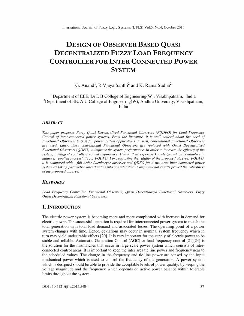
The modelling of a two area reheat thermal power system for load frequency control [9]-[16] is
investigated in this study as shown in Fig.1. The dashed lines show how the Area Control Error
(ACE) is computed within each area.
Consider the dynamic linear model of a two area LFC in state-space representation as described.
����� = ����� + ��� (1)
���� = ����� (2)
Where x(t) ∈ Rn, u(t)∈ Rm and y(t) ∈ Rp are the state vector, the control input vector and the
measurement output vector, respectively. Matrices A∈R�×�, B∈ R�×�and C∈ R�×�are known
constants.

International Journal of Fuzzy Logic Systems (IJFLS) Vol.5, No.4, October 2015
Figure.1. Two-area interconnected power system (TAIPS)
The state variable representation of the system has some advan
representation. The state vector x(t) contains enough information to completely summarize the
past behaviour of the system and the future
equation (1). The system properties
system can be studied by the
conceptual advantages.
In order to control a system, proper control schemes are to be designed to choose the input vector
u(t) so that the system behaves in an acceptable manner. Since the state vector x(t) contains all the
essential information about the system, it is reasonable to base the choice of u(t) solely on some
combinations of x(t). In other words u(t) is determined by relatio
(3)
where K ∈ R�×�is a constant matrix.
The analysis is simplified without loss of generality using
thermal turbines such that the power flow in the tie line can be considered as for Area 2.
Ptie2(t)= -Ptie2(t) is shown in Fig. 1.
Let xi(t),ui(t),di(t) and yi(t) (i=1,2) as state, control, load disturbance and o
Where
x1(t)= [Ptie1 f1 Pr1 Pg1 Xg1 �ACE
International Journal of Fuzzy Logic Systems (IJFLS) Vol.5, No.4, October 2015
area interconnected power system (TAIPS) block-diagram
The state variable representation of the system has some advantages over the transfer
representation. The state vector x(t) contains enough information to completely summarize the
of the system and the future behaviour is governed by the ordinary differential
properties are determined by the constant matrices A, B and C. Thus
studied by the well developed matrix theory having many notational and
In order to control a system, proper control schemes are to be designed to choose the input vector
t the system behaves in an acceptable manner. Since the state vector x(t) contains all the
essential information about the system, it is reasonable to base the choice of u(t) solely on some
combinations of x(t). In other words u(t) is determined by relation of the form u
is a constant matrix.
The analysis is simplified without loss of generality using a two area system consisting of reheat
thermal turbines such that the power flow in the tie line can be considered as for Area 2.
(t) is shown in Fig. 1.
(t) (i=1,2) as state, control, load disturbance and output vectors
ACE�dt ]T (4)
International Journal of Fuzzy Logic Systems (IJFLS) Vol.5, No.4, October 2015
39
transfer function
representation. The state vector x(t) contains enough information to completely summarize the
is governed by the ordinary differential
constant matrices A, B and C. Thus
many notational and
In order to control a system, proper control schemes are to be designed to choose the input vector
t the system behaves in an acceptable manner. Since the state vector x(t) contains all the
essential information about the system, it is reasonable to base the choice of u(t) solely on some
u(t) = −K x(t)
a two area system consisting of reheat
thermal turbines such that the power flow in the tie line can be considered as for Area 2.
utput vectors
(4)

International Journal of Fuzzy Logic Systems (IJFLS) Vol.5, No.4, October 2015
x2(t)= [f2 Pr2 Pg2 Xg2 �ACE�
ui(t)=Pci(t), di(t)=Pli(t)
yi(t)=[Ptiei fi Xg �ACE�dt]
T
As a result, the state space representation
area interconnected power system is obtained, where
)()()()( tDtButAxtx d++=
•
In (8), the integral of ACE’s are used
state values for frequencies and
control or Pole placement by state feedback has been extensively covered in the literature [1]
3. FUZZY OBSEVER
Fig. 2 shows a block diagram representation of the FQDFO implementation for LFC of a two area
interconnected power system. The flow of information
represented by the dotted lines. The two FO’s are decoupled from each other. Thus, there is no
transfer of data between them.
Figure.2. Block diagram of FQDFO’s for the two area interconnected power system
International Journal of Fuzzy Logic Systems (IJFLS) Vol.5, No.4, October 2015
dt ]T (5)
(6)
(7)
state space representation of an eleventh-order, 2-input, 2-disturbance for the two
area interconnected power system is obtained, where
(8)
In (8), the integral of ACE’s are used for controlling feedback variables to ensure zero steady
and tie line power for any step change in load disturbances.
Pole placement by state feedback has been extensively covered in the literature [1]
Fig. 2 shows a block diagram representation of the FQDFO implementation for LFC of a two area
interconnected power system. The flow of information from one area to another area is
represented by the dotted lines. The two FO’s are decoupled from each other. Thus, there is no
.2. Block diagram of FQDFO’s for the two area interconnected power system
International Journal of Fuzzy Logic Systems (IJFLS) Vol.5, No.4, October 2015
40
(5)
(6)
(7)
disturbance for the two
(8)
feedback variables to ensure zero steady
for any step change in load disturbances. Optimal
Pole placement by state feedback has been extensively covered in the literature [1]-[3].
Fig. 2 shows a block diagram representation of the FQDFO implementation for LFC of a two area
from one area to another area is
represented by the dotted lines. The two FO’s are decoupled from each other. Thus, there is no
.2. Block diagram of FQDFO’s for the two area interconnected power system

International Journal of Fuzzy Logic Systems (IJFLS) Vol.5, No.4, October 2015
41
A system involves many problems in monitoring, decision making, control and fault detection
which rely on the knowledge of time-varying parameters and state variables that cannot be
measured directly. In these situations, the estimation of parameters and states in dynamic systems
is an important requirement. Hence observers that use the input and output signals can be
employed to estimate the unknown states. Many estimation techniques are available for the
construction of observers for linear models such as the Kalman filter and its variants. However
there is no generalized procedure for the design of estimators for nonlinear systems as it involves
high computational costs. One such model which facilitates the stability analysis and observer
design can be represented by Takagi–Sugeno (TS) fuzzy model [11], a special dynamic nonlinear
model.
The system modelled in the state space using a state transition model can be mathematically
represented as
ẋ(t) = f(x(t), u(t), θ(t)) (9)
y(t) = h(x(t), u(t), ζ(t)) (10)
where, vector of the state variables is x, the measurement vector is y, the state transition function
is f, are describing the evolution of the states over time, the vector of the input or control variable
is u, the measurement function is h, relating the measurement to the states, ζ and θ are
(unknown/uncertain) parameters.
As the nonlinear systems were not described by the traditional methods, an accurate
approximation can be expected only in the surroundings of the equilibrium point. The TS model
is able to exactly approximate or represent to an arbitrary degree of accuracy. Based on Lyapunov
functions and linear matrix inequalities the structure facilitates observer design and stability
analysis using effective algorithms. A nonlinear system can be represented as a TS system. The
TS fuzzy model for nonlinear systems is of the form:
ẋ(t) = ∑ w����� �z�t�!�A�x�t� + B�u�t� + a�� (11)
y(t) = ∑ w����� �z�t�!�C�x�t� + c�� (12)
where m is the number of local rules or models, A�, B�, C� are the matrices and a�, c� are the biases
of the i)* local model, z(t) is the scheduling variables vector, which depend on the inputs, states,
measurements, etc., and w��z�t�!, i = 1, 2, . . . ,m are normalized membership functions, i.e.,
w��z�t�! ≥ 0 and ∑ w����� �z�t�! =1, ∀t∈ R.
3.1. TS fuzzy model:
Takagi and Sugeno proposed TS fuzzy model in 1985, consisting of an if-then rule base [10]. The
ith rule is described as
Model rule i:
If z� is Z�� and ... and z� is Z�� then y = F��z�
where the vector z has p components, z. , j = 1, 2, . . . , p, known as scheduling variables, as the
degree of activeness of the rules is determined by these values and depend on these values only.

International Journal of Fuzzy Logic Systems (IJFLS) Vol.5, No.4, October 2015
42
The setsZ.�s, j = 1, 2, . . . , p, i = 1, 2, . . ., m, where m is the number of rules of the fuzzy sets.
The value of z. belongs to a fuzzy set Z.� with a truth value of the membership function, ω�.: R →
[0, 1]. The truth value for an entire rule is determined as the minimum
φ�(z) = min.1ω�.�z.�2 (13)
or the algebraic product
φ�(z)= ∏ ω�.�z.��.�� (14)
The normalized form is
w��z� = φ4�5�
∑ φ4�5�6789
(15)
assuming that ∑ φ��z��.�� ≠ 0, i.e., that for any allowed combination of the scheduling variables at
least one rule has a truth value greater than zero. Hence w��z� is referred to as the normalized
membership function. Now using w��z�, the model output is represented in terms of z as
y = ∑ w��z�F��z����� (16)
When the successive rules (the functionsF�) also depend on exogenous variables, i.e., on variables
not appearing in the scheduling vector, the fuzzy model output is given as
y = ∑ w��z�F��z, θ����� (17)
where the vector of exogenous variables is θ and the number of these variables is p>.
3.2. Fuzzy observer:
The observer is of the form
x�? = ∑ w����� �z@��A�x@ + B�u + a� + L��y − y@�! (18)
y@ = ∑ w��z@��C�x@���� + c�� (19)
Where the estimated state vector is denoted by x@ ,the estimated measurement vector is denoted
by yC, the vector of the estimated scheduling variables is z@ (in the case of the scheduling vector
being estimated), and L�, i = 1, 2, . . . , m, are the observer gains to be designed. For an observer,
the state estimates should converge asymptotically to the original values. This can be taken as the
estimation error, e = x − x@.
As each observer has a local gain, instead of the full nonlinear system, the local model can be
taken to be observable i.e., the pairs (A�, C�) are observable[12].
The estimation error when using TS observer can be given as
e� = x� − x�? (20)

International Journal of Fuzzy Logic Systems (IJFLS) Vol.5, No.4, October 2015
43
e� = ∑ w����� �z@�∑ w.�z@��A� − L�C.��
.�� e +∑ w����� �z@�L�∑ �w.�z� − w.�z@���C.x + c.��
.�� +∑ �w��z� −w��z@���A�x + B�u + a��
�.�� (21)
This is the general expression when the measurement is linear and the scheduling variables
depend on the unmeasured state variables. There is a possibility that the scheduling vector does
not depend on the measured state variables also. Hence two cases are possible: 1) scheduling
vector depends on the measured state variable and 2) scheduling vector does not depend on the
measured states, i.e., it is an estimated vector.
3.2.1.Measured scheduling vector:
As the scheduling vector does not depend on the measured values, it can be taken as the observer.
Hence observer changes to
x�? = ∑ w����� �z��A�x@ + B�u + a� + L��y − y@�� (22)
y@ = ∑ w��z��C�x@���� + c�� (23)
Therefore, the error dynamics becomes
e� = ∑ ∑ w��z�w.�z��A� − L�C.�e�.��
���� (24)
By using the Lyapunov function, V = eFPe, with P = PF>0, and the change of variables M� =PL�, i=1,2,…,m, the observer is reduced to LMI (Linear Matrix Inequality).
3.2.2. Estimated scheduling vector:
The estimated values have to be used in the observer instead of the original values. For ease of
calculation, only the common measurement matrices, i.e., C�= C, i=1, 2,…m will be considered to
design similar observer gain matrices even if the design conditions are intricate. The observer for
the common measurement system becomes
x�? = ∑ w����� �z@��A�x@ + B�u + a� + L��y − y@�! (25)
y@ = Cx@ (26)
Therefore, the error dynamics changes to
e� = ∑ w��z@��A� − L�C�e + ∑ �w��z� − w��z@��w.�z��A�x + B�u + a������
���� (27)
4. RESULTS AND DISCUSSION
In this paper, the proposed technique is verified based on the results of Matlab / Simulink
implemented for the increase in demand of the first area IPD1 and second area IPD2. The
perturbation is given in both the areas at this condition and the step increase in demand is applied.
The frequency deviation of the first area If1 is shown in Figs. 3–8, using the proposed method,
the frequency deviations quickly driven back to zero and controller. Hence, when compared with
QDFO and Luenberger observer, FQDFO has the best performance in control and damping of
frequency in all responses.

International Journal of Fuzzy Logic Systems (IJFLS) Vol.5, No.4, October 2015
44
The Table 1 shows the robust performance for the above cases at a particular operating condition
numerically. Settling time, overshoot and undershoot for different operating points are studied.
Simulation results are shown for 10% band of step load change for the operating point of
Appendix A. Upon examination of Table 1, we can say that the performance of the proposed
FQDFO is better than the Luenberger observer and QDFO.
Table 1: f1(t) response performance in various control strategies
Operating
point Controller
Over shoot
(P.U)
Under shoot
( P.U)
Setting time
(sec)
1 Full order Luenberger
Observer
0.05211 -0.06554 5.213
Quasi Decentralized
Functional Observer
0.04539 -0.06088 5.111
Fuzzy Quasi Decentralized
Functional Observer
0.03901 -0.05404 5.033
2 Full order Luenberger
Observer
0.09419 -0.09907 4.994
Quasi Decentralized
Functional Observer
0.06718 -0.0868 4.796
Fuzzy Quasi Decentralized
Functional Observer
0.05021 -0.06943 4.526
3 Full order Luenberger
Observer
0.03961 -0.05186 6.369
Quasi Decentralized
Functional Observer
0.03681 -0.4921 6.251
Fuzzy Quasi Decentralized
Functional Observer
0.03391 -0.04543 6.121
4 Full order Luenberger
Observer
0.09231 -0.09644 6.321
Quasi Decentralized
Functional Observer
0.06 -0.07916 5.051
Fuzzy Quasi Decentralized
Functional Observer
0.04664 -0.06534 4.738
5 Full order Luenberger
Observer
0.0414 -0.05384 6.309
Quasi Decentralized
Functional Observer
0.03804 -0.05119 6.126
Fuzzy Quasi Decentralized
Functional Observer
0.03472 -0.04691 6.052
6 Full order Luenberger
Observer
0.06955 -0.08092 5.154
Quasi Decentralized
Functional Observer
0.0551 -0.07296 5.088
Fuzzy Quasi Decentralized
Functional Observer
0.04402 -0.06178 5.038
Fig.3 to Fig.8 are the comparison of f1 (t) responses for various observers in terms of nominal
values. The simulation results show that when compared to Luenberger observer and QDFO, the
proposed method is robust to change in the parameter of the system and has good performance in
all of the operating conditions

International Journal of Fuzzy Logic Systems (IJFLS) Vol.5, No.4, October 2015
45
Figure 3. Change in frequency with step increase in demand at operating point 1
Figure 4 Change in frequency with step increase in demand at operating point 2

International Journal of Fuzzy Logic Systems (IJFLS) Vol.5, No.4, October 2015
46
Figure. 5. Change in frequency with step increase in demand at operating point 3
Figure. 6. Change in frequency with step increase in demand at operating point 4

International Journal of Fuzzy Logic Systems (IJFLS) Vol.5, No.4, October 2015
47
Figure7. Change in frequency with step increase in demand at operating point 5
Figure 8. Change in frequency with step increase in demand at operating point6
5. CONCLUSIONS
In this paper, a new method is suggested to solve load frequency control problem using FQDFO
for a multi-area power system. The proposed observer is applied to a typical two area
interconnected reheat thermal power system with system parameter uncertainty. The simulation
results demonstrated that the designed observer guarantees the robust stability and performance. It
is tested for frequency tracking which is precised and disturbance attenuation under varying load
conditions and parameter uncertainities. To demonstrate the robustness of the proposed observer,
it is compared with QDFO and Luenberger observer in terms of settling time, maximum
overshoot and undershoots under different operating conditions.

International Journal of Fuzzy Logic Systems (IJFLS) Vol.5, No.4, October 2015
48
REFERENCES
[1] M. Darouach, “Full Order Observers for Linear Systems with Unknown Inputs”, IEEE Trans. Autom.
Control, vol. 39, no. 3, pp. 606–609, Mar. 1994.
[2] Hieu Trinh, Tyrone Fernand, “QuasiDecentralized Functional Observers for the LFC of
Interconnected Power Systems”, IEEE Transactions on Power Systems, 28, no. 3, Aug. 2013.
[3] H. Trinh, T. Fernand, “Functional Observers for Dynamical Systems”, Berlin, Germany: Springer
Verlag, 2012.
[4] K. R. Sudha, R. Vijaya Santhi, “Robust Decentralized Load Frequency Control of Interconnected
Power System with Generation Rate Constraint using Type-2 Fuzzy Approach”, Science Direct
Electrical Power and Energy Systems, 33, 699–707, 2011.
[5] M. Aldeen, J. Marsh, “DecentralisedObserver based Control Scheme for Interconnected Dynamical
Systems with Unknown Inputs”, IEEE Proceedings, Part D, Control Theory and Applications 146,
349–358, 1999.
[6] M. Aldeen, H. Trinh, “Load Frequency Control of Interconnected Power Systems via Constrained
Feedback Control Schemes”, Computers and Electrical Engineering 20, 71–88, 1994.
[7] B. Anderson, J. Moore, “Optimal Control: Linear Quadratic Methods”, Dover Publications, Mineola,
2007.
[8] Mendel JM, “Advances in Type-2 Fuzzy Sets and Systems”, Inform Science 177, 84–110, 2007.
[9] Venkateswarlu K, Mahalanabis AK, “Load Frequency Control using Output Feedback”, J Ins Eng
(India), pt. El-4 58, pp. 200–203,Feb.1987.
[10] M. Darouach and M. Boutayeb, Design of observers for descriptor systems,IEEE Transactions on
Automatic Control, vol. 40, pp. 1323-1327, 1995.
[11] M. Essabre , J. Soulami, and E. Elyaagoubi, Design of State Observer for a Class of Non linear
Singular Systems Described by Takagi-Sugeno Model, Contemporary Engineering Sciences, vol. 6,
2013, no. 3, 99-109,HIKARI Ltd.
[12] Michal Polanský, and Cemal Ardil” Robust Fuzzy Observer Design for Nonlinear Systems”
International Journal of Computer, Electrical, Automation, Control and Information Engineering
Vol:5, No:5, 2011
[13] X. J. Ma, Z. Q. Sun, “Analysis and design of fuzzy controller and Fuzzy observer” IEEE Trans.
Fuzzy Systems. 1998, vol. 6, no. 1, p. 41–51..
[14] Melin P, Castillo O, “A New Method for Adaptive Model based Control of Nonlinear Plants Using
Type-2 Fuzzy Logic and Neural Networks”, Proceedings of IEEE FUZZ conference, St. Louis, USA,
p. 420–25, 2003.
[15] T.Takagi, M. Sugeno, “Fuzzy identification of systems and itsapplications to modeling and control”
IEEE Transactions on Systems,Man and Cybernetics. 1985, vol. 1, no. 1, p. 116–132
[16] H.D. Mathur, ”Fuzzy based HVDC regulation controller for load frequency control of multi-area
system”International journal of Computer Aided Engineering and Technology Vol.4, No.1 pp.72 –
79, 2012.
[17] Meena Tushir, Smriti Srivastava, Yogendra Arya,”Application of hybrid fuzzy PID controller for
three-area power system with generation rate constraint” International journal of Energy Technology
and Policy , Vol.8, No.2 pp.159 – 173,2012.
[18] A.Soundarrajan & S.Sumathi, “Fuzzy based intelligent controller for LFC and AVR of a
owergenerating systems”, International journal of emerging technologies and applications
inengineering, technology and sciences, Vol.3, Issue.1, Jan, 2010.
[19] V.S. Vakula and K.R. Sudha, ”Design of differential evolution algorithm-based robust fuzzy logic
power system stabiliser using minimum rule base”, IET Generation, Transmission &
Distribution, Volume 6, Issue 2, p. 121 –132, February 2012.
[20] Ibraheem, Prabhat Kumar, and Dwarka P. Kothari “Recent Philosophies of Automatic Generation
Control Strategies in Power Systems” IEEE Transactions on power systems, vol. 20, no. 1, february
2005.
[21] KR Sudha, RV Santhi “Load frequency control of an interconnected reheat thermal system using
type-2 fuzzy system including SMES units”, International Journal of Electrical Power & Energy
Systems 43 (1), 1383-1392, 2012.

International Journal of Fuzzy Logic Systems (IJFLS) Vol.5, No.4, October 2015
49
[22] KR Sudha, YB Raju, AC Sekhar “Fuzzy C-Means clustering for robust decentralized load frequency
control of interconnected power system with Generation Rate Constraint” International Journal of
Electrical Power & Energy Systems 37 (1), 58-66, 2012
[23] R Vijaya Santhi, KR Sudha, S Prameela Devi ,“Robust Load Frequency Control of multi-area
interconnected system including SMES units using Type-2 Fuzzy controller, Fuzzy Systems (FUZZ),
2013 IEEE International Conference on, pp 1-7,2013
[24] R.Vijaya Santhi and K.R.Sudha, “Adaptive Type-2 Fuzzy Controller For Load Frequency Control Of
An Interconnected Hydro Thermal System Including SMES Units” International Journal of Fuzzy
Logic Systems (IJFLS) Vol.4, No.1, January 2014.
[25] Singha, Joyeeta, and Rajkumar Joydev Borah. "Recent Advances in Microbend Sensors in Various
Applications."
[25] Semwal, Vijay Bhaskar, Pavan Chakraborty, and G. C. Nandi. "Less computationally intensive fuzzy
logic (type-1)-based controller for humanoid push recovery." Robotics and Autonomous Systems 63
(2015): 122-135.