design of multi-loop control systems - computer science...

1

Design of Multi-loop control systems

Consider a single loop system as shown in Fig.1.

Fig.1

Suppose controller is fixed, substantial changes inpK invariably lead to deteriorate the

control system response (see Figure 2).

Fig.2

Now consider a 2 2× control system in Fig. 3

Fig.3

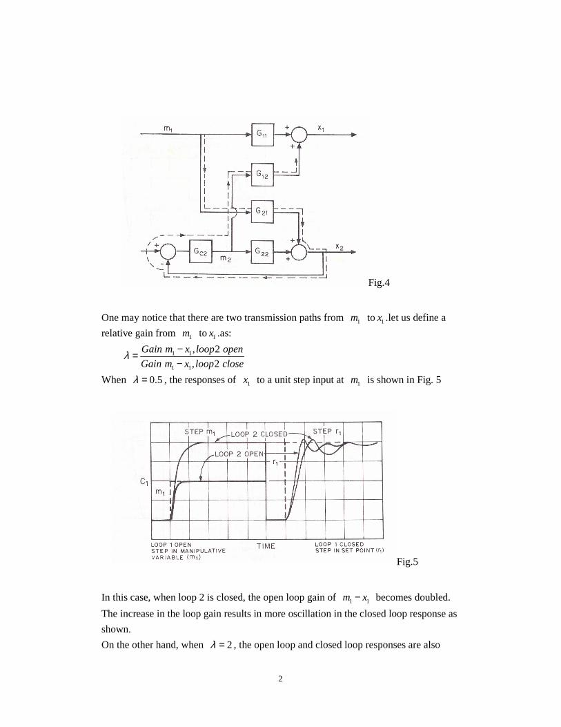
Let us consider open loop 1 (Fig.4)

2

Fig.4

One may notice that there are two transmission paths from 1m to 1x .let us define a

relative gain from 1m to 1x .as:

1 1

1 1

, 2

, 2

Gain m x loop open

Gain m x loop closeλ −=

−

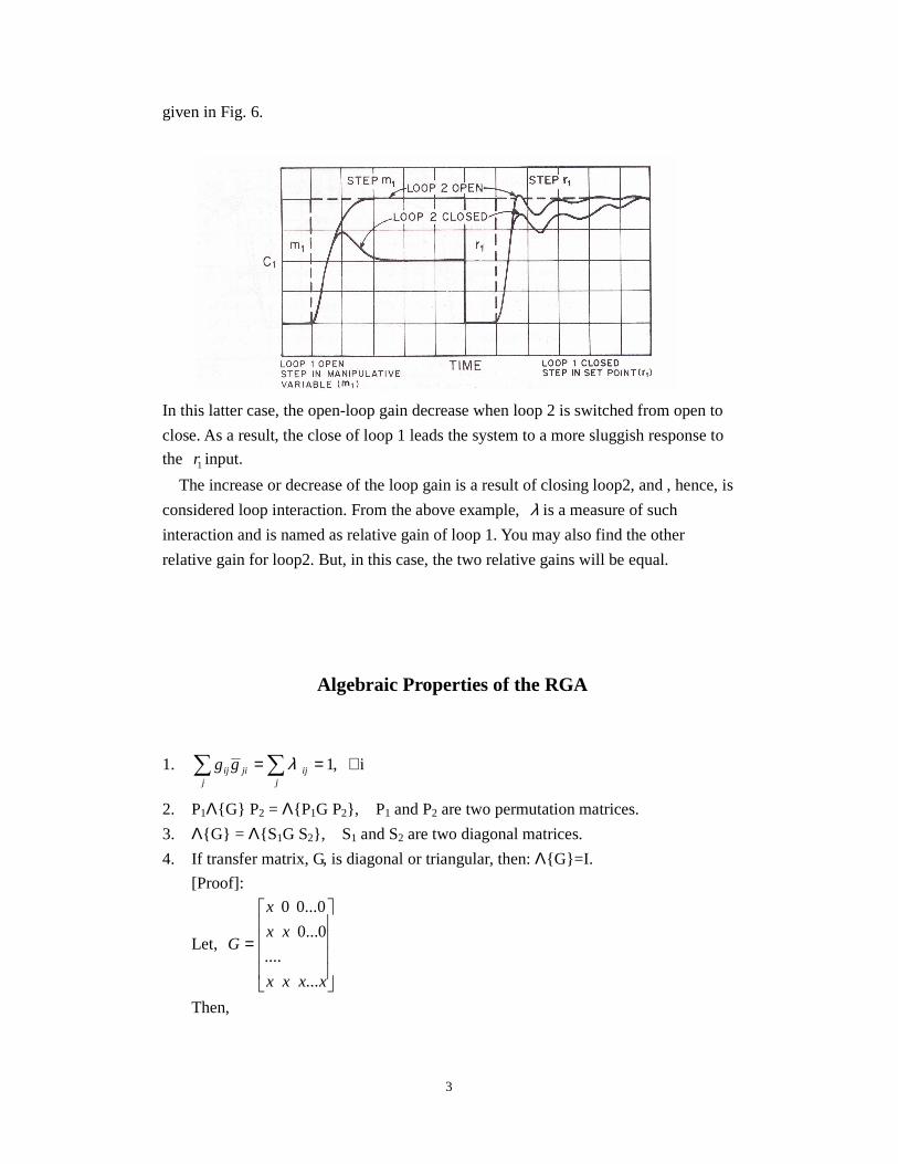
When 0.5λ = , the responses of 1x to a unit step input at 1m is shown in Fig. 5

Fig.5

In this case, when loop 2 is closed, the open loop gain of 1 1m x− becomes doubled.

The increase in the loop gain results in more oscillation in the closed loop response as

shown.

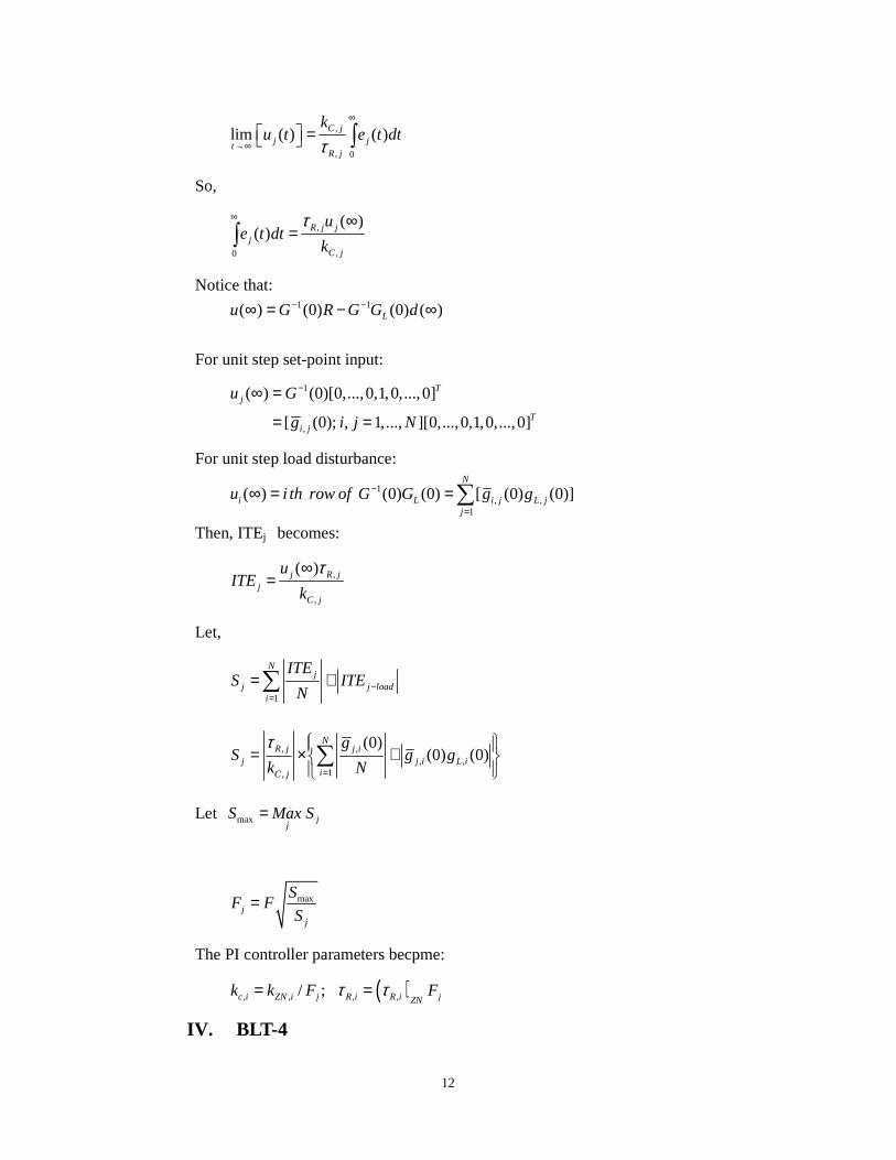
On the other hand, when 2λ = , the open loop and closed loop responses are also

3

given in Fig. 6.

In this latter case, the open-loop gain decrease when loop 2 is switched from open to

close. As a result, the close of loop 1 leads the system to a more sluggish response to

the 1r input.

The increase or decrease of the loop gain is a result of closing loop2, and , hence, is

considered loop interaction. From the above example, λ is a measure of such

interaction and is named as relative gain of loop 1. You may also find the other

relative gain for loop2. But, in this case, the two relative gains will be equal.

Algebraic Properties of the RGA

1. i ,1 ∀==∑∑j

ijjij

ij gg λ

2. P1ΛG P2 = ΛP1G P2, P1 and P2 are two permutation matrices.

3. ΛG = ΛS1G S2, S1 and S2 are two diagonal matrices.

4. If transfer matrix, G, is diagonal or triangular, then: ΛG=I.

[Proof]:

Let,

=

xxxx

xx

x

G

...

....

0...0

0...0 0

Then,

4

==−

xxxx

xx

x

GG

...

....

0...0

0...0 0

1

Thus, ij , 0 ij ≠∀== λjiij gg

and, ij , 1 ii =∀== λiiii gg

So, Λ =I

5. ij

ij

ji

ji

g

dg

g

gdij λ−=

]det[

]det[)1(

]det[

][

G

G

G

Aadjg

ijji

ij

+−==

22

2

2 )](det[

]det[

)](det[

]det[)1( ]det[

jiij

ij

ij

ijji

ij

ij

ji ggG

G

gG

Gdg

Gd

dg

gd−==

−−=

+

ij

ijij

ij

ijijjiijji

ji

ji

g

dg

g

dgggdgg

g

gd λ−=−=−=

5. ij

ij

ij

ij

g

gdd

g

dgd

ij

ij

ij

ijij

ij

ij

1

and ,) 1(

λλ

λλ

λλλ −

=−=

[Proof];

jiijjiijjiij gdggdgdgg +=⇒= ijij λλ

ij

ijij

ji

ji

ij

ij

jiij

jiijjiij

g

dg

g

gd

g

dg

gg

gdggdgd) 1()(

ij

ij λλλ

−=+=+

=⇒

or,

ij

ij

ij

ij

ij

ij

ijji

ji

ij

ij

g

gd

g

gd

g

gd

g

dgd

1 )

11(

ij

ij

−=−=+

=⇒

λλ

λλλ

5

RGA-implications:

1. Pairing loops on λij values that are positive and close to 1.

2. Reasonable Pairings: 0.5 < λij< 4.0

3. Pairing on negative λij values results in at least one of the following;

a. Closed loop system is unstable,

b. Loop with negative λij is unstable,

c. Closed loop system becomes unstable if loop with negative is λij turned off.

4. Plants with large RGA-elements are always ill-conditioned. (i.e., a plant with a

large γ(G) may have small RGA-elements)

5. Plants with large RGA-elements around the crossover frequency are fundamentally

difficult to control because of sensitivity to input uncertainties.

-----decouplers or other inverse-based controllers should not be used for plants

with large RGA-elements.

6. Large RGA-element implies sensitivity to element-by-element uncertainty.

7. If the sign of RGA-element changes from s=0 to s=∞ , then there is a RHP-zero

in G or in some subsystem of G.

8. The RGA-number can be used to measure diagonal dominance:

RGA-number = || Λ(G)-I ||min.

For decentralized control,, pairings with RGA-number at crossover frequency

close to one is preferred.

9. For integrity of whole plant, we should avoid input-output pairing on negative

RGA-element.

10. For stability, pairing on an RGA-number close to zero at crossover frequency is

preferred.

6

The Relative Disturbance Gain (RDG)

Ref: Galen Stanley, Maria Marino-Galarraga, and T. J. McAvoy, Shortcut

Operability Analysis. 1. The relative disturbance gain, I&EC, Process Des. Dev.

1985,24, 1181-1188

The use of RDG:

1. To decide if interaction resulting from a disturbance is favorable or unfavorable.

2. To decide whether or not decoupling should be used and what type of decoupling

structure is best.

1 11 1 12 2 1

2 21 1 22 2 2

F

F

y k m k m k d

y k m k m k d

= + += + +

1 2

1 1

11,

F

y m

m k

d k

∂ = − ∂

1 2

1

,y y

m

d

∂ ∂

is derived when both y1 and y2 are held still:

1 11 1 12 2 1

2 21 1 22 2 2

0

0F

F

y k m k m k d

y k m k m k d

= + + == + + =

(2)

so that:

[ ]2 21 1 222

1Fm k m k d

k= − − (3)

Substitute Eq.(3) into E.(2), we have:

12 21 12 211 1 1

22 22

0FF

k k k kk m k d

k k

− + − =

Thus,

1 2

12 21

1 22 12 2 1 22

12 21 11 22 12 21,11

22

FF

F F

y y

k kk

m k k k k kk kd k k k kk

k

− +∂ − = = ∂ − −

(4)

7

So,

1 2

1 2

1

, 11 12 2 1 22 11 22 12 2 1 221

1 1 11 22 12 21 1 22 11 22 12 21

,

12 2 1 22 11 22 12 2

1 22 11 22 12 21 1 22

=- 1

y y F F F F

F F

y m

F F F

F F

m

d k k k k k k k k k k k

m k k k k k k k k k k kd

k k k k k k k k

k k k k k k k k

β

λ

∂ ∂ − −

= = − × = ×∂ − − ∂

−× = − −

(5)

Similarly, we have:

1 2

1 2

1

, 21 11

1 2 11

,

1y y F

F

y m

m

d k k

m k kd

β λ

∂ ∂

= = − ∂ ∂

2 12 1 1 2 1 22

1 22 1 12

1 F F

F F

k k k k

k k k k

β λ β λ βλ λ λ

− −= − = ⇒ = ×

1 2 11

2 21

Similarly, F

F

k k

k k

λ βλ−

⇒ = ×

So, 2 1 2 11 1 22

1 2 21 12

1F F

F F

k k k k

k k k k

λ β λ βλ λ

− −× = = × × ×

2 1 11 22

21 12

1 1

k k

k k

λ β λ βλ λ λ− −

⇒ = = −

or,

( )( )1 2 ( 1)β λ β λ λ λ− − = −

( ) ( ) ( )( )( )

1 12 2

1 1 1 1

1 1( 1) ( 1)

β λ βλ λ λ λβ λ β λ λβ λ β λ β λ λ β

− −− −− = ⇒ = + = =− − − −

It can be shown that:

8

11

1

22

2

Multi-loop e area and

SISO idealy decoupled e area

Multi-loop e area


β

β

∝

∝

2 12 2 1 22 21

11 1 22 2 2 1 12 21

(1 )

(1 )(1 )c c

c c c c

F G G F G Ge

d G G G G G G G G

− +=

+ + − (6)

If d is a unit step, then the area under e1 curve is given as:

2 1 22 22 12

2 2 2 12 1 221 10

1 11 2 22 2 10 1 11 22 12 2112 21

1 2 2 1 1 11 22

1 122 1

1 11 22

lim ( )

1

c F cF

R R F F

sc c c c c

R R R R R

RF F

c

k k k kk k

k k k ke dt e s

k k k k k k k k k k kk kk k

kk k

k k k

τ τ

τ τ τ τ τ

τλ

∞

→

−−

= = = − −

= −

∫

On the other hand, when loop 2 is opened, the area under e1becomes:

'1 1

1 '1110

o R F

c

ke dt

kk

τ∞

= −∫

Thus,

9

1 ' '

0 1 11 2 12 11 1 1' '

1 1 22 11 11

0

1c cR F R

o c F cR R

e dtk kk k

fk k k k

e dt

τ τλ β βτ τ

∞

∞

= − × − = × =

∫

∫

Similarly, we have:

2 '

0 222 2 2'

222

0

cR

o cR

e dtk

fk

e dt

τ β βτ

∞

∞ = × =∫

∫

Notice that the PI parameters in the interacting loops are used to be more conservative

than those in single loops. In another words,

1 21; 1f f≥ ≥

The multi-loop control should be beneficial when the sum of absolute values of the

Remarks:

1. If λ is assumed not vary with frequency, and the process under study is FOPDT,

λ>1, f1 lies in the range 1< f1 <2, while 0.5<l<1, f1 lies in the range 1< f1 <3.

2. When f1 =1, β is equal to the ratio of response areas.

3. If β is small and f1 =is close to one, then the interacting control is favored for that

particular disturbance.

4. If β is large, the interacting control is un favorable for that particular disturbance.

The Relative Gain for Non-square Multivariable Systems (J.C. Chang and C.C. Yu, CES Vol.45, pp. 1309-1323 1990)

Consider a non-square MV system.

1 1( ) ( ) ( )m m n ny s G s u s× × ×=

Define Moore-Penrose pseudo-inverse of the matrix ( )G s as:

( ) 1( ) ( )T TG s G G G s

−+ =

Then, under close-loop control, the steady-state control input will be:

(0) du G y+= and (0)iij

j CL

ug

y+ ∂

= ∂ .

Thus, the non-square relative gain is defined similarly to the square RGA, that is:

10

1

(0) (0)T

i i

j jOL CL

y yG G

u u

−

+ ∂ ∂

Λ = = ⊗ ∂ ∂

%

Properties of the non-square RGA

1. Row sum of Λ% :

[ ] 1 21 1 1

(1), (2), , ( ) , , , ,

Tn n n

j j mjj j j

RS rs rs rs m λ λ λ= = =

= =

∑ ∑ ∑% % %L L ;

Where, ( ) (0) (0)ii

rs i G G+ =

2. [ ] [ ]1 21 1 1

(1), (2), , ( ) , , , , 1, 1, , 1

Tn n n

T

j j jnj j j

CS cs cs cs n λ λ λ= = =

= = =

∑ ∑ ∑% % %L L L

Where, ( ) (0)ii

cs i G G+ = ; (Note: 1( )T TG G G G G G I+ −= = )

3. 0 ( ) 1, 1,2, ,rs i i m≤ ≤ ∀ = L

4. 1 1

( ) ( )m n

i j

rs i cs i n= =

= =∑ ∑

Note: 1 1 1 1 1 1

( ) ( )m m n n m n

ij iji i j j i j

rs i cs j nλ λ= = = = = =

= = = =∑ ∑∑ ∑∑ ∑% %

5. Non-square RGA is invariant under input scaling, but is variant under output

scaling:

( ) ( )( )TT

GS GS G G+ + ⊗ = ⊗ ( ) ( )( )TT

SG SG G G+ + ⊗ ≠ ⊗

6. Let 1P and 2P are permutation matrices. Then, 1 2 1 2( ) ( )PGP P G PΛ = Λ% %

A. Multi-loop BLT-Tuning:

I. BLT-1 method:

a. Calculate the Ziegler-Nichol settings for each PI controller by using the

diagonal element of G, i.e. gi,i.

b. Assume a detuning factor “F”, and calculate controller settings for loops.

( ), , , ,/ ;c i ZN i R i R i ZNk k F Fτ τ= =

c. Define: ( ) ( ) ( )1 deti i c iW I G Gω ω ω = − + +

11

d. Calculate the closed-loop function Lc(iω):

( )( )

( )

20log1

ic i

i

WL

Wω

ωω

=+

e. Calculate the detuning factor F until the peak in the Lc log modulus curve is

equal to 2N, that is:

( )

( )

20log 21

icm

i

WL N

WMax ω

ω ω

= = +

II. BLT-2

a. Find BLT-1 PI controllers.

b. Choose a second detuning factor FD. FD should be greater than one.

c. Compute τD,j as:

( ),

,

D j ZND j

DF

ττ =

d. Calculate W(iω) and Lc(iω).

e. Change FD until maxCL is minimized, maintaining FD > 1. The trivial case may

result where maxCL is minimized for DF = ∞ , i.e., no derivative action.

f. Reduce F in the P and I modes, until max 2CL N= .

III. BLT-3

The objective is to estimate the level of imbalance in detuning the BLT-1

controller and compensate for it.

Consider the PI controller:

,, 0

1(0)

t

j j C j j jR j

u u k e e dtτ

= + +

∫ ; (0) 0ju =

At steady state,

12

,

, 0

lim ( ) ( )C jj j

tR j

ku t e t dt

τ

∞

→∞ = ∫

So,

,

,0

( )( ) R j j

jC j

ue t dt

k

τ∞ ∞=∫

Notice that: 1 1( ) (0) (0) ( )Lu G R G G d− −∞ = − ∞

For unit step set-point input:

1

,

( ) (0)[0,...,0,1,0,...,0]

[ (0); , 1,..., ][0,...,0,1,0,...,0]

Tj

Ti j

u G

g i j N

−∞ =

= =

For unit step load disturbance:

1, ,

1

( ) (0) (0) [ (0) (0)]N

i L i j L jj

u i th row of G G g g−

=

∞ = =∑

Then, ITEj becomes:

,

,

( )j R jj

C j

uITE

k

τ∞=

Let,

1

Nj

j j loadi

ITES ITE

N −=

= +∑

, ,, ,

1,

(0)(0) (0)

NR j j i

j j i L iiC j

gS g g

k N

τ=

= × + ∑

Let max jj

S Max S=

maxj

j

SF F

S=

The PI controller parameters becpme:

( ), , , ,/ ;c i ZN i j R i R i jZNk k F Fτ τ= =

IV. BLT-4

13

a. BLT-3 is used to get individual PI controllers as described above.

b. BLT-2 procedure is used with individual FD factors for each loop:

max,D j D

j

SF F

S=

V. Tyreus Load-Rejection Criterion (TLC)

The best variable pairing is the one that gives the smallest magnitudes for each

element of X,(i.e. Xi) of the following:

( )1( ) ( )

[ ]i C L iX I GG G Lω ω

−= +

VI. Summary

B. Parallel-design method---Modified Z-N methods for

TITO Processes

This method is based on A modified Z-N method for SISO control system. To derive

this modified Z-N method, ageneral formulation is to start with a given point of the

Nyquist curve of the process:

( )( ) pjp pG j r e π ϕω − += (1)

And to find a regulator GR

BLT-1--- PI, equal Fi

BLT-3---PI, unequal Fi

BLT-2---PID, equal Fi

BLT-4-----PID, unequal Fi

14

1( ) 1R D

R

G j k jj

ω ωττ ω

= + −

(2)

To move this point to ( )sjsB r e π ϕ− += (3)

An amplitude margin (i.e. gain margin) design corresponding to 0sϕ = and

1s

m

rA

= .

A phase margin design corresponds to 1sr = and s mϕ ϕ=

From Eqs.(1)~Equ.(3), we have: ( )( ) p Rsjj

s p Rr e r r e π ϕ ϕπ ϕ − + +− + = , so that

sR

p

rr

r= and R s pϕ ϕ ϕ= −

In other words,

( )1( ) 1 cos sinRj

R D R R R R RR

G j k j r e r jrj

ϕω ωτ ϕ ϕτ ω

= + − = = +

Or,

( )cos cossR R s p

p

rk r

rϕ ϕ ϕ= = − and ( )1

tanD s pR

ωτ ϕ ϕτ ω

− = −

The gain is uniquely determined. Only one equation determines Rτ and Dτ .

Let D Rτ ατ= , where α is often chosen as 0.25α ≈ . Another method to specify α

is as follows:

0.413

3.302 1α

κ=

+, where

(0)

( )c

g

g jκ

ω=

From ( )11tanD s p

R

ωτ ϕ ϕτ ω

− − = −

, Dτ can be solved to obtain:

21tan( ) 4 tan ( )

2D s p s pτ ϕ ϕ α ϕ ϕω = − − + + −

and

1R Dτ τ

α=

Consider a stable 2 2× process :

15

1 11 12 1

2 21 22 2

( ) ( ) ( ) ( )

( ) ( ) ( ) ( )

y s g s g s u s

y s g s g s u s

=

1 1

2 2

( ) ( ) 0

( ) 0 ( )

c s c s

c s c s

=

2 12 21 12 211 11 11 1

2 22 2 221

c g g g gg g g

c g c g−= − = −+ +

12 212 22 1

1 11

g gg g

c g−= −+

Let

( ) ( )aiji ai i iA r e g jπ ϕ ω− += =

( ) ( ) ( )biji bi i i i iB r e g j c jπ ϕ ω ω− += =

1

( ) 1 ; 1,2i DiRi

c j k j ij

ω ωττ ω

= + + =

Take PI controller as example.

( )( ) 1 tan( ) ; 1,2i ci bi aic j k j iω ϕ ϕ= − − =

And, ( )( ) cos( ) aiji i ci bi ai big j k r e π ϕω ϕ ϕ − += −

16

( ) ( )

( )

(1 tan( ))

cos( ) sin( ) (1 tan( ))

ia ia

ai bi

j jai ci bi ai bi

jbi bi biai bi ai bi ci bi ai

ai ai ai

ci

r e k j r e

r r re j k j

r r r

rk

π ϕ π ϕ

ϕ ϕ

ϕ ϕ

ϕ ϕ ϕ ϕ ϕ ϕ

− + − +

−

⋅ − − =

⇓

= − + − = − −

⇓

=

( ) ( )

cos( )

( ) cos( ) cos( )ia ia

biai bi

ai

j jbici i ai bi ai bi ai bi

ai

r

rk g j r e r e

rπ ϕ π ϕ

ϕ ϕ

ω ϕ ϕ ϕ ϕ− + − +

−

⋅ = − ⋅ = − ⋅

By setting i equal one and two, one will obtain two equations with kc1 and kc2 as

unknowns, and, thus, can be solved. But, there are very tedious procedures to find the

controller gains (such as:such kc1 and kc2) and frequency 11ω and 22ω that satisfy the

phase criteria. (see the reference: I&EC Res. 1998, 37, 4725-4733, Q-G Wang, T-H

Lee, and Y. Zhang)

C. Independent design method

---IMC Multi-loop PID Controller

17

( ) 1

, , ; 1,...,C i i i iG G f i n−

−= =

The stability is guaranteed for any stable IMC filter that satisfies either of the

following:

,*

,

,,

( )( ) ( ) ; 1,2,...,

( )

i i

i R i

i jj j i

g if i f i i n

g i

ωω ω

ω≠

< = =∑

,*

,

,,

( )( ) ( ) ; 1,2,...,

( )

i i

i C i

j ij j i

g if i f i i n

g i

ωω ω

ω≠

< = =∑

Imc Row interaction measure [Economou and Morari]

,

,

*, ,

( )1

( ) ; 01 ( ) ( )

i jj j i

iR i i j

j

g i

R if i g i

ωω ω

ω ω≠= = ≤ ≤ ∞

+

∑

∑

,

,

*, ,

( )1

( ) ; 01 ( ) ( )

j ij j i

iC i j i

j

g i

C if i g i

ωω ω

ω ω≠= = ≤ ≤ ∞

+

∑

∑

For significant interaction: *0.5 , 1 1i iR C f≤ ≤ ⇒ <

f1

f2

[(g11) -]-1

[(g22)-]-1

G

g11

g22

_

_

_

_

18

For small interaction: *0.0 , 0.5 1i iR C f≤ ≤ ⇒ >

D. Chien-Huang-Yang’s multi-loop PID---with no

proportional and derivative kicks

1. Controllers for SISO loop:

Controller: 1( ) ( ) [ ( ) ( )] ( )C D

R

u s k y s r s y s sy ss

ττ

= − + − −

/( )

1 /( )

C R p

C R p

k s Gy

r k s G

ττ

=+

a. Time constant dominant processes:

Re; slope of the initial unit step response

Ls

PG Rs

−

= =

Re (1 )Ls

P

R LsG

s s

− −= ≈

2 22

2 2

1 1

1.414 1( ) 1

(1.414 ) ; 1.414

( 1.414 )

C CRR R

C

CC R C

C C

y Ls Ls

r s sL s L s

Rk

Lk L

R L L

τ ττ τ τ

τ τ ττ τ

− −= ≈+ +

− + − +

+⇒ = = +

+ +

b. Deadtime dominant processes:

e (1 )

1 1

LsP P

P

k k LsG

s sτ τ

− −= ≈+ +

19

2

2 2

2

2 2

2

1

1

1

1.414 1

1.4141 ;

1.414

1.414

R RR R

C P C P

C C

C CC

P C C

C CR

y Ls

rL s L s

k k k k

Ls

s s

Lk

k L

L

L

τ τ ττ τ

τ ττ τ τ ττ τ τ

τ τ τ τττ

−=

− + + − +

−≈+ +

− + +⇒ =

+ +

− + +⇒ =

+

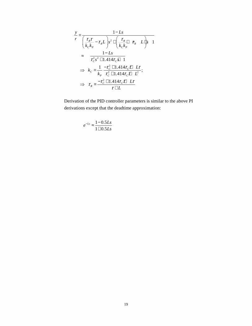
Derivation of the PID controller parameters is similar to the above PI

derivations except that the deadtime approximation:

1 0.5

1 0.5Ls Ls

eLs

− −≈+

22

2. Controllers for multi-loop system

1,2 2,1 1,11,1

1 1,1 2,2loop 2 closed

0 ; 1( )

k k gyAt g

u k k RGAω

λ

→ = − =

1,11 loop 2 closed

;y

At gu

ω → ∞ =

a. For RGA>1, multi-loop controller tuning based on the process

model in the main loop should provide satisfactory closed loop

results. This is because:

b. For RGA < 1,

( ), ,based on main loop( )C i C i ik k RGA λ=

( ), based on main loop

,,( )

R i

R ii iRGA

ττ

λ=

( ), , ,based on main loop( )D i D i i iRGAτ τ λ=

The closed-loop time constant is chosen according to the value of L/τ in three different ranges, that is: L/τ < 0.2, 0.2 < L/τ < 0.5, and L/τ >

0.5.

For details, see the original paper.

.

IX. Robustness of Closed-loop System.

The final pairing and the controller tuning is checked for robustness by

plotting DSO and DSI as functions of frequency, [Doyle and Stein]. The

singular values below 0.3-0.2 indicate a lack of stability robustness.

( )

( )

1

( ) ( )

1

( ) ( )

[ ]

[ ]

i C i

i C i

DSO I GG

DSI I G G

ω ω

ω ω

σ

σ

−

−

= +

= +

23

E. Design Method based on Passivity

1. Hardware simplicity and relative effortlessness to achieve failure tolerant design,

multi-loop control is the most widely used strategy in the industrial process

control.

2. Current multi-loop control design approaches can be classified into three

categories: detuning methods (Luyben, 1986), independent design methods

(Skogestard and Morari, 1989), and sequential design methods (Mayne, Chiu and

Arkun, 1992).

3. Loop interactions have to be taken into considerations, as they may have

deteriorating effects on both control performance and closed-loop stability.

4. It is desirable if the multi-lop control system is decentralized unconditionally

stable (i.e., any subset of the control loops can be independently to an arbitrary

degree or even turned off without endangering close-loop stability.

5. Independent design is based on the basis of the paired transfer function while

satisfying some stability constraints due to process interactions.

6. Perhaps the mostwidely used decentralized stability conditions are those

µ-interaction measure.

7. Passivity Concept:

The rate of change of the stored energy in the tank is less than the power supplied

to it.

Potential energy stored in the tank: 21 12 2( )S h Ah gh A ghρ ρ= =

Increment of potential energy per unit time: ( ) ( ) ( )iw t F t gh tρ=

The rate of change of the storage function:

0v i vdS

C gh h gF h C gh h w w hdt

ρ ρ ρ= − + = − + < ∀ >

The rate of change of the stored energy in the tank is less than the power

supplied to it. Therefore this process is said to be strictly passive.

h

Inlet Flowrate Fi

Fo

Outlet Flowrate

24

Passive(Willems 1972): if a non-negative storage function S(x) can be found s.t.:

S(0)=0 and 0

0( ) ( ) ( ) ( )

t T

tS x S x y u dτ τ τ− ≤ ∫ for all t>t0≥0, x0, x∈ X, u∈ U.

Strictly passive: if 0

0( ) ( ) ( ) ( )

t T

tS x S x y u dτ τ τ− < ∫

Where, y is the output of a system, u is the input to the system.

KYP Lemma

Nonlinear control affine systems (Hill & Moylan 1976) ( ) ( )

( )

where n m m

x f x g x u

y h x

x X R , u U R , y Y R

= +=

∈ ⊂ ∈ ⊂ ∈ ⊂

&

The process is passive if

( ) ( ) ( )

( ) ( ) ( ) ( )

0,T

f

TT

g

S xL S x f x

x

S xL S x g x h x

x

∂= ≤

∂∂

= =∂

KYP Lemma

A linear system (Willems 1972) G(s):=(A,B,C,D) is passive if there exists a

positive definite matrix P such that:

0T T

T T

A P PA PB C

B P C D D

+ −≤

− − −

The system is strictly passive if

0T T

T T

A P PA PB C

B P C D D

+ −<

− − −

Definition:

An LTI system S: G(s) is passive if :

(1) G(s) is analytic in Re(s)>0;

(2) G(jw)+G*(jw)≥0 for all that jw is not a pole of G(s);

(3) If there are poles of G(s) on the imaginary axis, they are non-repeated and the

residue matrices at the poles are Hermitian and positive semi-definite.

G(s) is strictly passive if:

(1) G(s) is analytic in Re(s) ≥ 0; (2) G(jw)+G*( jw)>0 ( , )ω∀ ∈ −∞ ∞ .

25

Theorem 1: For a given stable non-passive process with a transfer function matrix

G(s), there exists a diagonal, stable, and passive transfer function matrix

W(s)=w(s)I such that H(s)=G(s)+W(s) is passive.

[Proof]:

* * *min min( ( ) ( )) ( ( ) ( ) ( ( ) ( ))H j H j G j G j W j W jλ ω ω λ ω ω ω ω+ = + + +

Since both (G+G*) and (W+W*) are Hermitian, from the Weyl inequality, we

have:

* * *

min min min

*min

( ( ) ( )) ( ( ) ( )) ( ( ) ( ))

= ( ( ) ( )) 2Re( ( ))

H j H j G j G j W j W j

G j G j W j

λ ω ω λ ω ω λ ω ωλ ω ω ω

+ ≥ + + +

+ +

Thus, if:

*min

1Re( ( )) ( ( ) ( ))

2W j G j G jω λ ω ω≥ +

H(s) can be render passive. On the other hand, if

*min

1Re( ( )) ( ( ) ( ))

2W j G j G jω λ ω ω> +

H(s) will be strictly passive.

Properties of Passive Systems:

A passive system is minimum phase. The phase of a linear process is within

[-90º, 90º]

Passive systems are Lyapunov stable

A passive system is of relative degree < 2

Passive systems can have infinite gain (e.g., 1/s)

Passivity Theorem :

If G1 is strictly passive and G2 is passive, then the closed-loop system is L2

stable.

A strictly passive process can be stabilized by any passive controller

26

(including multi-loop PID controllers) even if it is highly nonlinear and/or

highly coupled

Control design based on passivity

Excess or shortage of passivity of a process can be used to analyse whether

this process can be easily controlled

Passivity based controllability study

A non-passive process can be made passive using feedforward and/or feedback

passification:

The excess or shortage of passivity can be quantified using:

Input Feedforward Passivity (IFP) (Sepulchre et al 1997) - If a system

G with a negative feedforward of νI is passive, then G has excessive

input feedforward passivity, i.e., G is IFP(ν).

Output Feedback Passivity (OFP) (Sepulchre et al 1997) - If a system

G with a positive feedback of ρI is passive, then G has excessive

output feedback passivity, i.e., G is OFP (ρ).

Agin, use the following figure:

If G1 is IFP(ν) and G2 is OFP(ρ), then the closed-loop system is stable if ρ+ν>0.

In other words, a processs shortage of passivity can be compensated by another

process’s excess of passivity.

Passivity Index

The excessive IFP of a system G(s) can be quantified by a frequency dependent

Gfb

G

Gff

G

27

passivity index

min1

[ ( ), ] [ ( ) *( )]2F G s G j G jν ω λ ω ω

∆ +

=

Assume the true process is ( ) ( ) ( )TG s G s s= + ∆

The passivity index of the true process can be estimated as

* *min

* *min min

1 1( ( )) ( ) ( ) ( ) ( )

2 2

1 1 ( ) ( ) ( ) ( )

2 2

= ( ( )) ( ( ))

TG j j j G j G j

j j G j G j

G j j

ν ω λ ω ω ω ω

λ ω ω λ ω ω

ν ω ν ω

= − ∆ + ∆ + +

≤ − ∆ + ∆ − − +

+ ∆

Properties of the Passivity Index

1. Comprises gain & phase information of the uncertainty

2. Always no greater than the maximum singular value.

max[ ( ), ] [ ( )] for any F s j Rν ω σ ω ω∆ ≤ ∆ ∈

σ

Passivity index

Maximum gain

j

∆(σ)∆(σ)∆(σ)∆(σ)

28

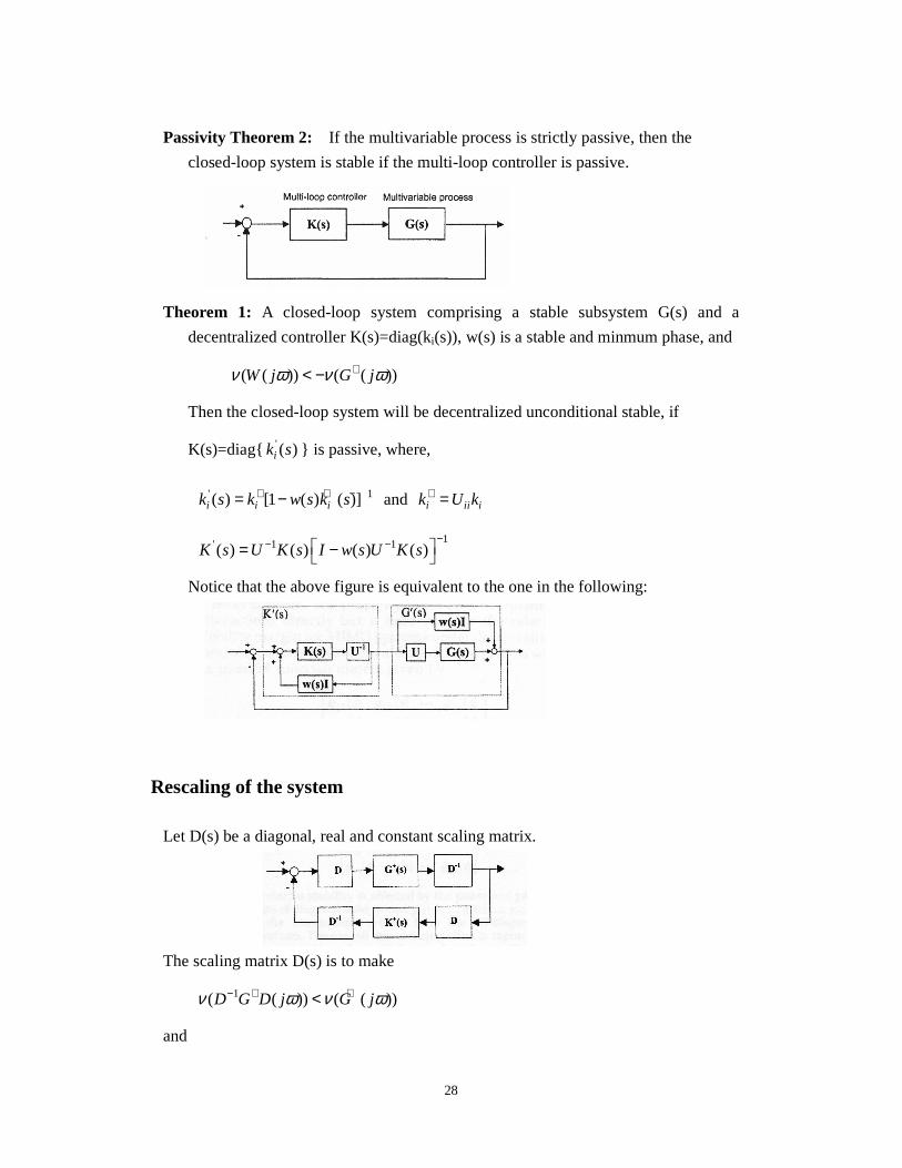
Passivity Theorem 2: If the multivariable process is strictly passive, then the

closed-loop system is stable if the multi-loop controller is passive.

Theorem 1: A closed-loop system comprising a stable subsystem G(s) and a

decentralized controller K(s)=diag(ki(s)), w(s) is a stable and minmum phase, and

( ( )) ( ( ))W j G jν ω ν ω+< −

Then the closed-loop system will be decentralized unconditional stable, if

K(s)=diag '( )ik s is passive, where,

' 1( ) [1 ( ) ( )]i i ik s k w s k s+ + −= − and i ii ik U k+ =

1' 1 1( ) ( ) ( ) ( )K s U K s I w s U K s

−− − = −

Notice that the above figure is equivalent to the one in the following:

Rescaling of the system

Let D(s) be a diagonal, real and constant scaling matrix.

The scaling matrix D(s) is to make

1( ( )) ( ( ))D G D j G jν ω ν ω− + +<

and

29

1 1(0) (0) 0D G D D G D+− + − + + >

Design procedures:

1. Find matrix U and calculate ( )G s+ .

2. Check the pairing. Examine the proposed pairing using DIC condition:

(0) (0) 0T

G M M G+ + + >

3. Use matrix M obtained in the step 2 to derive D, 1/ 2D M=

4. Calculate 1( ( ) )D G j Dν ω− + for different frequency points. These frequency

points form a set [ ]0, EωΩ ∈ where Eω is the frequency which is high enough

sych tant 1( ( ) ) 0D G j Dν ω− + → for Eω ω> .

5. For each loop of the controller, solve problem:

,min( )

ci Ri

ik τ

γ−

such that

,,

11

11 ( ) 1

i

ii c iR i

jG j k

j

γω

ωτ ω

+ +

<

+ +

and

,2, 2

,

( ), , 1, ,

1 ( )

c i sR i

c i s

kR i n

k

ν ωτ ω

ν ω ω

+

+≥ ∀ ∈ = −

L

6. Obtain the final controller settings: , ,c i ii c ik U k +=

This method is limited to open-loop stable processes.

30

Robust Stability Condition

If the uncertainty is passive, then the controller is only required to render system T

strictly passive to achieve robust stability even if ∆ is very large.

If the uncertainty’s passivity index is bounded by

( ) ( )( ), ( ), ,F Fs W sν ω ν ω ω∆ ≥ − ∀ ∈R

where W(s) is minimum phase, the closed-loop system will be robust stable if

system

1( )[ ( ) ( )]T s I W s T s −−

is strictly passive.

The basic idea:

1. Characterise the uncertainty in terms of passivity using IFP or OFP.

2. Derive the robust stability condition for systems with uncertainties bounded by

their passivity indices.

3. Develop a systematic procedure to design the robust controller which satisfies

the above stability condition.

Passivity Based Robust Control Design

Blended approach

Design a controller that satisfies the small gain condition at high

frequencies and satisfies the passivity condition at low frequencies

(Bao, Lee et al 1998)

Based on the bilinear transformation

∆∆∆∆

T

( ) ( ) R∈∀−≥∆ ωωνων ,),(),( sWs FF

31

Multi-objective control design

Design a controller that satisfies the passivity condition for robust

stability and achieves H∞ control performance (Bao, Lee et al 2000,

2003)

Based on KYP lemma and Semi-Definite Programming

Example:

Passivity index

F. Design by Sequential Loop Closing

Advantages of sequential design: 1. Each step in the design procedure involves designing only one SISO controller.

2. Limited degree of failure tolerance is guaranteed: If stability has been achieved

110-40 -

1

10-2 1 10 0 1

10+2 10+41

4

-0-0.03.0

-0.-0.020

-0.0

0.0 0 0.0

0.0.0202 0.0.0404 P

as

si

vit

+−

+

++−

+= −−

−−

135

12.0

138

094.0)145)(148(

101.0

160

126.0

)(88

126

s

e

s

ess

e

s

e

sGss

ss

(rad/min

32

after the design of each loop, the system will remain stable if loop fail or are taken

out of service in the reverse order of they were designed.

3. During startup, the system will be stable if the loops are brought into service in the

same order as they have been designed.

4.

Problems with sequential design: 1. The final controller design, and thus the control quality achieved, may depend on

the order in which the controllers in the individual loops are designed.

2. Only one output is usually considered at a time, and the closing of subsequent

loops may alter the response of previously designed loops, and thus make iteration

necessary.

3. The transfer function between input uk and output yk may contain RHP zeros that

do not corresponding to the RHP zeros of G(s).

Notations:

1. G(s): the n n× matrix of the plant, ( ) ( ); , 1, , ijG s g s i j n= = L

2. ( ) ( ); 1, , iC s diag c s i n= = L

3. 1 1( ) ; ( )S I GC H I S GC I GC− −= + = − = +

4. ( ); 1, , iiG diag g s i n= =% L

5. 1

( ); 1, , ; 1, , 1i

ii i

S diag s s i n diag i ng c

= = = =+

% L L

6. ( ); 1, , ; 1, , 1

ii ii

ii i

g cH diag h s i n diag i n

g c= = = =

+% L L

7. 1 ; , 1, , ijGG i j nγ−Γ = = =% L

8. 1dCLDG GG G−= %

9. 1( )E G G G−= − % %

10. ; C ; k kG CG

= =

M M

L O L O

11. ( ) ( )1 1; k k k k k k k kS I G C H G C I G C

− −= + = +

12. 0 0ˆˆ ; ; 1, 2,

00

k kk k

ii

H SH S i k K N

sh

= = = + +

L

% %

33

( ) ( ) ( ) ( )

( ) ( ) ( )

1 1

11

11

1 1 1

1

( ) [ ( ) ]

( )

( )

S I GC I GC G G C

I G G C I GC I GC

I G G G I GC

I GC I EH S I EH

GC I GC

− −

−−

−−

− − −

−

= + = + + −

= + − + +

= + − +

= + +

+

= +

% %

% % %

% % %

% %% %

% %

Design procedures:

In each of the following step, ( ) 11 ˆ( ) ; ( ) k k k k k kS S I E H E G G G−−= + = −

) ))

Determine ic such that p DW SWis minimized.

Step 0. Initialization. Determine the order of loop closing by estimating the

required bandwidth in each loop. Also estimate the individual loop designs

in terms of H% .

Step 1. Design of controller c1 by considering output 1 only. In this case, we have

ˆk kG G= % and ˆ

kH H= %

Step k. Design of controller ck by consider outputs 1 to k. Here,

ˆ , ; 1, 2, ,k k iiG diag G g i k k n= = + +% L and

1,ˆ ; , 1, ,k k iH daig H h i k k n−= = +% L

34

Sequential Design Using Relay feedback Tests of Shen and Yu

The relay feedback system for SISO auto-tuning is as shown in the follwing figure:

When constant cycles appear after the system has been activated, the ultimate gain

and ultimate frequency of the open-loop system can be approximated by measuring

the magnitude and period (see the following figure) and by the following equations:

4 2

; u uu

hK

a P

πωπ

= =

The Z-N tuning method can be used to determine the controller parameters:

PI Controller: 0.45 , /1.2,

PID Controller: 0.60 , /1.2, 1.25c u R u

c u R u D u

K K P

K K P P

ττ τ

= == = =

Or, use the Tyreus-Luyben’s formula to give more conservative response:

PI Controller: / 3.2, 2.2 ,

PID Controller: / 2.2, 2.2 , / 6.3c u R u

c u R u D u

K K P

K K P P

ττ τ

= == = =

To avoid the difficult mathematics envolved in the formulation of sequential

design, Shen and Yu suggested to use the relay-feedback test as shown in the

following figure:

35

The controller for a 2 2× system is suggested:

,PI Controller: / 3, 2 c c ZN R uK K Pτ= =

Analysis: The sequential design is derived by considering the multi-loop control system as

coupled SISO loops. For a 2 2× system as example, the equivalent SISO loops are:

1 1,1 21

( ) ( ) 1 (1 ) ( )( )

g s g s h ssλ

= − −

2 2,2 11

( ) ( ) 1 (1 ) ( )( )

g s g s h ssλ

= − −

Where, C,i ,

, ,

g(s) ; 1 2

1i i

iC i i i

gh i ,

g g= =

+

Notice that, if there is damping in 1 2or g g , this damping should come from either

1 2or h h . According to tis study, a closed system having an FOPDT process and a

modified ZN tuned PI controller will result in a closed-loop system (i.e. 1h and 2h )

having damping factor greater than 0.6. It is thus postulate that the open-loop transfer

functions 1 2( ) and ( )g s g s can be approximated by:

22 2

1

1( )

12 1p p s

p

k sG s e

ss sθτ

ττ τζ−+

= ⋅ ⋅++ +

Then, the stability region of the equivalent SISO loops are explored with the

parameters: 1, 0 ~ 10, 1, 5, 0.1 ~ 1, / 0.02 ~ 0.2p p pkτ τ τ ζ θ τ= = = = = . The results

36

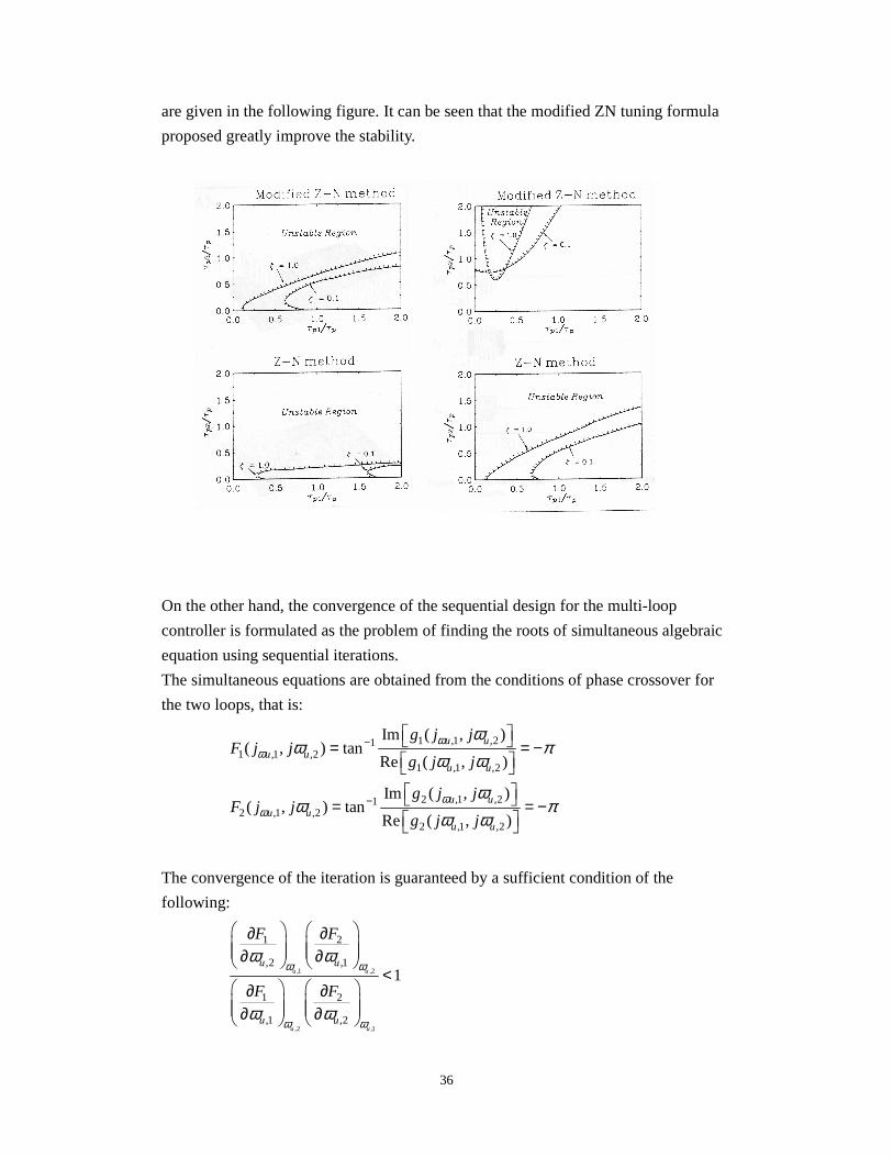
are given in the following figure. It can be seen that the modified ZN tuning formula

proposed greatly improve the stability.

On the other hand, the convergence of the sequential design for the multi-loop

controller is formulated as the problem of finding the roots of simultaneous algebraic

equation using sequential iterations.

The simultaneous equations are obtained from the conditions of phase crossover for

the two loops, that is:

1 ,1 ,211 ,1 ,2

1 ,1 ,2

2 ,1 ,212 ,1 ,2

2 ,1 ,2

Im ( , )( , ) tan

Re ( , )

Im ( , )( , ) tan

Re ( , )

u uu u

u u

u uu u

u u

g j jF j j

g j j

g j jF j j

g j j

ωω

ωω

ωω π

ω ω

ωω π

ω ω

−

−

= = −

= = −

The convergence of the iteration is guaranteed by a sufficient condition of the

following:

,1 ,2

,2 ,1

1 2

,2 ,1

1 2

,1 ,2

1u u

u u

u u

u u

F F

F F

ω ω

ω ω

ω ω

ω ω

∂ ∂ ∂ ∂

< ∂ ∂ ∂ ∂

37

The procedures of this proposed sequential design are summarized with the flow

chart as shown.

1

Design of Multi-loop control systems

Consider a single loop system as shown in Fig.1.

Fig.1

Suppose controller is fixed, substantial changes inpK invariably lead to deteriorate the

control system response (see Figure 2).

Fig.2

Now consider a 2 2× control system in Fig. 3

Fig.3

Let us consider open loop 1 (Fig.4)

2

Fig.4

One may notice that there are two transmission paths from 1m to 1x .let us define a

relative gain from 1m to 1x .as:

1 1

1 1

, 2

, 2

Gain m x loop open

Gain m x loop closeλ −=

−

When 0.5λ = , the responses of 1x to a unit step input at 1m is shown in Fig. 5

Fig.5

In this case, when loop 2 is closed, the open loop gain of 1 1m x− becomes doubled.

The increase in the loop gain results in more oscillation in the closed loop response as

shown.

On the other hand, when 2λ = , the open loop and closed loop responses are also

3

given in Fig. 6.

In this latter case, the open-loop gain decrease when loop 2 is switched from open to

close. As a result, the close of loop 1 leads the system to a more sluggish response to

the 1r input.

The increase or decrease of the loop gain is a result of closing loop2, and , hence, is

considered loop interaction. From the above example, λ is a measure of such

interaction and is named as relative gain of loop 1. You may also find the other

relative gain for loop2. But, in this case, the two relative gains will be equal.

Algebraic Properties of the RGA

1. i ,1 ∀==∑∑j

ijjij

ij gg λ

2. P1ΛG P2 = ΛP1G P2, P1 and P2 are two permutation matrices.

3. ΛG = ΛS1G S2, S1 and S2 are two diagonal matrices.

4. If transfer matrix, G, is diagonal or triangular, then: ΛG=I.

[Proof]:

Let,

=

xxxx

xx

x

G

...

....

0...0

0...0 0

Then,

4

==−

xxxx

xx

x

GG

...

....

0...0

0...0 0

1

Thus, ij , 0 ij ≠∀== λjiij gg

and, ij , 1 ii =∀== λiiii gg

So, Λ =I

5. ij

ij

ji

ji

g

dg

g

gdij λ−=

]det[

]det[)1(

]det[

][

G

G

G

Aadjg

ijji

ij

+−==

22

2

2 )](det[

]det[

)](det[

]det[)1( ]det[

jiij

ij

ij

ijji

ij

ij

ji ggG

G

gG

Gdg

Gd

dg

gd−==

−−=

+

ij

ijij

ij

ijijjiijji

ji

ji

g

dg

g

dgggdgg

g

gd λ−=−=−=

5. ij

ij

ij

ij

g

gdd

g

dgd

ij

ij

ij

ijij

ij

ij

1

and ,) 1(

λλ

λλ

λλλ −

=−=

[Proof];

jiijjiijjiij gdggdgdgg +=⇒= ijij λλ

ij

ijij

ji

ji

ij

ij

jiij

jiijjiij

g

dg

g

gd

g

dg

gg

gdggdgd) 1()(

ij

ij λλλ

−=+=+

=⇒

or,

ij

ij

ij

ij

ij

ij

ijji

ji

ij

ij

g

gd

g

gd

g

gd

g

dgd

1 )

11(

ij

ij

−=−=+

=⇒

λλ

λλλ

5

RGA-implications:

1. Pairing loops on λij values that are positive and close to 1.

2. Reasonable Pairings: 0.5 < λij< 4.0

3. Pairing on negative λij values results in at least one of the following;

a. Closed loop system is unstable,

b. Loop with negative λij is unstable,

c. Closed loop system becomes unstable if loop with negative is λij turned off.

4. Plants with large RGA-elements are always ill-conditioned. (i.e., a plant with a

large γ(G) may have small RGA-elements)

5. Plants with large RGA-elements around the crossover frequency are fundamentally

difficult to control because of sensitivity to input uncertainties.

-----decouplers or other inverse-based controllers should not be used for plants

with large RGA-elements.

6. Large RGA-element implies sensitivity to element-by-element uncertainty.

7. If the sign of RGA-element changes from s=0 to s=∞ , then there is a RHP-zero

in G or in some subsystem of G.

8. The RGA-number can be used to measure diagonal dominance:

RGA-number = || Λ(G)-I ||min.

For decentralized control,, pairings with RGA-number at crossover frequency

close to one is preferred.

9. For integrity of whole plant, we should avoid input-output pairing on negative

RGA-element.

10. For stability, pairing on an RGA-number close to zero at crossover frequency is

preferred.

6

The Relative Disturbance Gain (RDG)

Ref: Galen Stanley, Maria Marino-Galarraga, and T. J. McAvoy, Shortcut

Operability Analysis. 1. The relative disturbance gain, I&EC, Process Des. Dev.

1985,24, 1181-1188

The use of RDG:

1. To decide if interaction resulting from a disturbance is favorable or unfavorable.

2. To decide whether or not decoupling should be used and what type of decoupling

structure is best.

1 11 1 12 2 1

2 21 1 22 2 2

F

F

y k m k m k d

y k m k m k d

= + += + +

1 2

1 1

11,

F

y m

m k

d k

∂ = − ∂

1 2

1

,y y

m

d

∂ ∂

is derived when both y1 and y2 are held still:

1 11 1 12 2 1

2 21 1 22 2 2

0

0F

F

y k m k m k d

y k m k m k d

= + + == + + =

(2)

so that:

[ ]2 21 1 222

1Fm k m k d

k= − − (3)

Substitute Eq.(3) into E.(2), we have:

12 21 12 211 1 1

22 22

0FF

k k k kk m k d

k k

− + − =

Thus,

1 2

12 21

1 22 12 2 1 22

12 21 11 22 12 21,11

22

FF

F F

y y

k kk

m k k k k kk kd k k k kk

k

− +∂ − = = ∂ − −

(4)

7

So,

1 2

1 2

1

, 11 12 2 1 22 11 22 12 2 1 221

1 1 11 22 12 21 1 22 11 22 12 21

,

12 2 1 22 11 22 12 2

1 22 11 22 12 21 1 22

=- 1

y y F F F F

F F

y m

F F F

F F

m

d k k k k k k k k k k k

m k k k k k k k k k k kd

k k k k k k k k

k k k k k k k k

β

λ

∂ ∂ − −

= = − × = ×∂ − − ∂

−× = − −

(5)

Similarly, we have:

1 2

1 2

1

, 21 11

1 2 11

,

1y y F

F

y m

m

d k k

m k kd

β λ

∂ ∂

= = − ∂ ∂

2 12 1 1 2 1 22

1 22 1 12

1 F F

F F

k k k k

k k k k

β λ β λ βλ λ λ

− −= − = ⇒ = ×

1 2 11

2 21

Similarly, F

F

k k

k k

λ βλ−

⇒ = ×

So, 2 1 2 11 1 22

1 2 21 12

1F F

F F

k k k k

k k k k

λ β λ βλ λ

− −× = = × × ×

2 1 11 22

21 12

1 1

k k

k k

λ β λ βλ λ λ− −

⇒ = = −

or,

( )( )1 2 ( 1)β λ β λ λ λ− − = −

( ) ( ) ( )( )( )

1 12 2

1 1 1 1

1 1( 1) ( 1)

β λ βλ λ λ λβ λ β λ λβ λ β λ β λ λ β

− −− −− = ⇒ = + = =− − − −

It can be shown that:

8

11

1

22

2

Multi-loop e area and


Multi-loop e area


β

β

∝

∝

2 12 2 1 22 21

11 1 22 2 2 1 12 21

(1 )

(1 )(1 )c c

c c c c

F G G F G Ge

d G G G G G G G G

− +=

+ + − (6)

If d is a unit step, then the area under e1 curve is given as:

2 1 22 22 12

2 2 2 12 1 221 10

1 11 2 22 2 10 1 11 22 12 2112 21

1 2 2 1 1 11 22

1 122 1

1 11 22

lim ( )

1

c F cF

R R F F

sc c c c c

R R R R R

RF F

c

k k k kk k

k k k ke dt e s

k k k k k k k k k k kk kk k

kk k

k k k

τ τ

τ τ τ τ τ

τλ

∞

→

−−

= = = − −

= −

∫

On the other hand, when loop 2 is opened, the area under e1becomes:

'1 1

1 '1110

o R F

c

ke dt

kk

τ∞

= −∫

Thus,