design of low-sweep wings for maximum...

Design of Low-Sweep Wings for Maximum Range

Timothy M. Leung∗ and David W. Zingg†

Institute for Aerospace Studies, University of Toronto, Toronto, Ontario, M3H 5T6, Canada

An efficient Newton-Krylov algorithm for high-fidelity aerodynamic shape optimizationis used to design low-sweep wings for maximum range at transonic speeds. In this approach,the steady flow solution is obtained using the Newton method with pseudo-transient con-tinuation. The objective function gradient is computed using the discrete-adjoint method.Linear systems from both the flow and adjoint systems are solved using a preconditionedKrylov method. A quasi-Newton optimizer is used to find the search direction. It is coupledwith a line-search algorithm. Our single-point optimization results show that it is possibleto design shock-free unswept wings at Mach numbers and lift coefficients comparable tothe operating conditions of modern transonic transport aircraft. Robust wing designs forlow-sweep and unswept wings under the same operating conditions are obtained throughmulti-point optimization.

I. Introduction

In the design of future generations of civil transport aircraft, optimizing the wing configuration to maxi-mize range is of particular interest to designers. The range maximization problem is analogous to minimizingfuel burn at a fixed range. The amount of fuel consumed in flight has a profound impact on the operat-ing cost for the operator (airline), as fuel cost is currently the largest single expense for airlines globally.1

Fuel burn also has significant environmental impact, through the production of greenhouse gas emissions,particularly carbon dioxide (CO2) and nitrogen oxides (NOx). In the 1990s, when jet fuel was substantiallyless expensive, designs favoured operating at higher speeds for passenger comfort, and to reduce labour costduring flight. However, given the rising cost of fuel and increasing environmental regulations in recent years,this philosophy is being revisited.

Advances in high-fidelity computational fluid dynamics (CFD) techniques over the past decades, as wellas the development of CFD-based aerodynamic shape optimization techniques in the design process, haveallowed engineers to examine the range maximization problem more closely. We are particularly interestedin the aerodynamic optimization of unswept and low-sweep wings that can operate within a flight envelopesimilar to the highly-swept wings currently used by civil transport aircraft. Low-sweep wings are appealingbecause they can have reduced structural weight, which is another important factor in maximizing range,and the potential for natural laminar flow. The goal is to optimize for robust, shock-free designs at transonicMach numbers.

Our study is motivated by the work of Jameson et al.2 Their primary results show that even withaerodynamic shape optimization alone, the range of a low-sweep wing operating at lower Mach numberis comparable to a highly-swept wing at higher Mach number. In our current work, we revisit the rangemaximization problem using the Newton-Krylov algorithm based on Nemec and Zingg3 and Leung andZingg.4 Our study includes an improved curve fit to account for the engine’s thrust specific fuel consumptionas a function of Mach number, as well as using a flexible geometry parameterization method using basis-splines (B-splines). We also examine the effect of robust design. The objective is to assess potential benefitsof unswept and low-sweep wings and to find the maximum Mach numbers for robust shock-free operation asa function of sweep angle under a particular set of geometric constraints.∗Research Engineer, AIAA Member†Professor and Director, Tier 1 Canada Research Chair in Computational Aerodynamics, J. Armand Bombardier Foundation

Chair in Aerospace Flight, Associate Fellow AIAA

1 of 11

American Institute of Aeronautics and Astronautics

II. Optimization Problem

A. Problem Formulation

The goal of aerodynamic shape optimization is to find a set of design variables X and state variables Q suchthat a scalar objective function J minimized:

minXJ (X ,Q) (1)

The optimization is subject to both geometric constraints:

Cj(X ) ≤ 0 (2)

as well as the flow constraint:R(X ,Q) = 0 (3)

In the present study, the flow constraint is defined by the discrete steady Euler equations governing com-pressible inviscid flow.

B. Objective Function

We formulate the objective function J based on the Breguet range equation, which specifies the range R ofan aircraft under a cruise-climb flight profile:

R =V

TSFCL

Dln(Wi

Wf

)(4)

where V is the speed of the aircraft, L/D is the aircraft’s lift-to-drag ratio (aerodynamic efficiency), TSFCis the engine’s thrust specific fuel consumption, and Wi and Wf are initial and final weights of the aircraft.For high-bypass-ratio turbofan engines used on commercial transport aircraft, TSFC varies roughly linearlywith M at transonic speeds. We use the relationship by Mattingly:5

TSFC ∝ 0.45M + 0.40 (5)

The exact relationship between TSFC and M depends on the specific engine configuration. Under the cruise-climb flight profile, the aircraft operates at a constant speed V and lift coefficient CL. As weight decreasesduring flight, the altitude increases such that the lift L generated is always equal to the weight. For anaerodynamic shape optimization, the effects of weights Wi and Wf are ignored for now. It should be notedthat these weights are important factors for a full aero-structural optimization.

Substituting non-dimensional quantities into (4), the range of an aircraft scales with a range factor R:

R =M

TSFCCL

CD(6)

For optimization at a fixed Mach number, R can be maximized by maximizing the lift-to-drag ratio at afixed CL. For this type of problem, we use the lift-constrained drag minimization objective function:

J0 = ωL

(1− CL

C∗L

)2

+ ωD

(1− CD

C∗D

)2

(7)

The targets in lift and drag (C∗L, C∗D) as well as the weights (ωL, ωD) are specified by the user. We find thevalues ωL = 100 and ωD = 1.0 to be effective based on previous experience.4 If the target lift is attainable andtarget drag is not, then the lift constraint appears as a penalty term. Therefore, C∗D should be a value thatis physically unattainable to ensure that the final drag is minimized. Once we have obtained the optimizedlift-to-drag ratio, we can compute the range factor R.

2 of 11


C. Multi-Point Optimization

For multi-point optimization with Np operating conditions, the objective function is the weighted sum of alloperating points:6

JT =Np∑i=1

ωiJi (8)

This weighted sum is an approximation of a weighted integral I of the objective function over a range ofMach numbers:

I =∫ M2

M1

P (M)J [X ,Q(M)] dM (9)

where the user-specified weighting function P (M) reflects the relative importance attached by the designerto each Mach number in this range. In (8), the weights ωi combine the weighting function P (M), as well asthe Newton-Cotes rule that is used to approximate (9). For P (M) = 1, if we select equally spaced operatingpoints between M1 and M2, with the first and last operating point at M1 and M2 respectively, and applythe trapezoidal rule, we obtain the following weights:

ωi =

0.5 i = 11.0 i = 2 . . . Np − 10.5 i = Np

(10)

D. Geometric Constraints

We have implemented two geometric constraints: a volume constraint to limit the change in the volumeenclosed by the wing, and a thickness constraint to maintain minimum thickness at specified locations of thewing. Both are expressed as penalty terms in the objective function:

J = J0 + Jp,V + Jp,T (11)

For volume constraint, the penalty term Jp,V is added when the volume V deviates from the initial volumeV0:

Jp,V = ωV

(1− V

V0

)2

(12)

The penalty weight ωV is supplied by the user. We choose a value of ωV = 50.0. For thickness constraints,we specify a minimum thickness at fixed relative positions along the chord (x/c) and semi-span (y/(b/2))on the wing. The penalty term is added if thickness at the i-th constraint location ti is below the minimumthickness t∗i . The contributions from all thickness constraints are summed and multiplied by a user suppliedweight ωT:

Jp,T = ωT

∑i

(1− ti

t∗i

)2

(13)

We use a penalty weight of ωT = 40.0.

III. Algorithm Description

A. Flow Analysis

The governing equations for the optimization are the Euler equations, which are discretized on multi-blockstructured grids. In our parallel strategy, each block in the grid and the corresponding component of Qis distributed to a separate processor. Second-order centred differencing is applied at interior nodes, whilefirst-order one-sided differencing is used at boundaries and block interfaces. For numerical stability, we use ascalar dissipation model based on the JST scheme.7,8 Boundary conditions and the coupling between blocksat the interfaces are enforced using simultaneous approximation terms (SATs).9

Discretization of the steady Euler equations produces a set of nonlinear algebraic equations, which canbe written as:

R(Q) = 0 (14)

3 of 11


Beginning with an initial guess Q(0) based on free-stream properties, and applying the Newton method, wesolve a linear system in the form: (

∂R∂Q

)(n)

∆Q(n) = −R(Q(n)) (15)

The left-hand-side matrix is the flow Jacobian. The flow vector Q is updated after each iteration, andthe linear system is solved again until ‖R(Q)‖2 is reduced by more than 10 orders of magnitude. At eachiteration, (15) is solved using the Krylov method Flexible Generalized Minimal Residual (FGMRES).10,11

Note that when using a Krylov method, only matrix-vector products with the flow Jacobian are required.These can be approximated by one-sided differencing:(

∂R∂Q

)v ≈ R(Q + εv)−R(Q)

ε(16)

leading to a Jacobian-free approach. The linear system is right-preconditioned using an approximate-Schurpreconditioner based on Refs. 9 and 12.

To improve the stability of the Newton method during the start-up phase, the flow solver uses anapproximate-Newton method, where a first-order Jacobian A1 replaces the flow Jacobian in (15). A pseudo-transient time step is also added for globalization:

∆t(n)i =

∆t(n)ref

Ji(1 + 3√Ji)

(17)

where the reference time step for iteration n is defined as

∆t(n)ref = A(B)n (18)

Values of A = 0.1 and B = 1.5 are used. In summary, during the approximate-Newton start-up phase, thelinear system solved at each iteration n is given by:[

T(n) + A(n)1

]∆Q(n) = R(n) (19)

where T(n) is a diagonal matrix containing the reciprocal of the local time steps. The flow solver switchesto the Newton method when the residual has been reduced by one order of magnitude:

‖R(n)‖2‖R(0)‖2

< 0.10 (20)

During the Newton phase, the reference time step is based on Mulder and van Leer:13

∆t(n)ref = max

[α

(‖R(n)‖2‖R(0)‖2

)−β,∆t(n−1)

ref

](21)

We find α = 1.0 and β = 1.75 found to be satisfactory values for a wide range of problems. As the residualdecreases, the time step approaches infinity, and the full Newton step is recovered.

B. Gradient Computation

A fast and accurate evaluation of the objective function gradient G is necessary for an effective gradient-basedoptimizer. The gradient can be expressed in terms of the design variables X and adjoint variables Ψ:

G =∂J∂X−ΨT ∂R

∂X(22)

where Ψ is the solution to the discrete adjoint equation:(∂R∂Q

)TΨ =

∂J∂Q

T

(23)

4 of 11


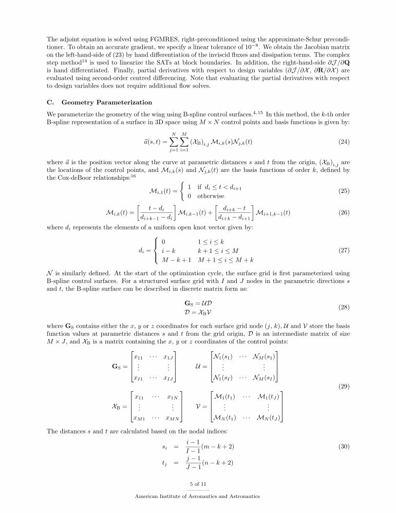
The adjoint equation is solved using FGMRES, right-preconditioned using the approximate-Schur precondi-tioner. To obtain an accurate gradient, we specify a linear tolerance of 10−8. We obtain the Jacobian matrixon the left-hand-side of (23) by hand differentiation of the inviscid fluxes and dissipation terms. The complexstep method14 is used to linearize the SATs at block boundaries. In addition, the right-hand-side ∂J /∂Qis hand differentiated. Finally, partial derivatives with respect to design variables (∂J /∂X , ∂R/∂X ) areevaluated using second-order centred differencing. Note that evaluating the partial derivatives with respectto design variables does not require additional flow solves.

C. Geometry Parameterization

We parameterize the geometry of the wing using B-spline control surfaces.4,15 In this method, the k-th orderB-spline representation of a surface in 3D space using M ×N control points and basis functions is given by:

~a(s, t) =N∑j=1

M∑i=1

(XB)i,jMi,k(s)Nj,k(t) (24)

where ~a is the position vector along the curve at parametric distances s and t from the origin, (XB)i,j arethe locations of the control points, and Mi,k(s) and Nj,k(t) are the basis functions of order k, defined bythe Cox-deBoor relationships:16

Mi,1(t) =

1 if di ≤ t < di+1

0 otherwise(25)

Mi,k(t) =[

t− didi+k−1 − di

]Mi,k−1(t) +

[di+k − t

di+k − di+1

]Mi+1,k−1(t) (26)

where di represents the elements of a uniform open knot vector given by:

di =

0 1 ≤ i ≤ ki− k k + 1 ≤ i ≤MM − k + 1 M + 1 ≤ i ≤M + k

(27)

N is similarly defined. At the start of the optimization cycle, the surface grid is first parameterized usingB-spline control surfaces. For a structured surface grid with I and J nodes in the parametric directions sand t, the B-spline surface can be described in discrete matrix form as:

GS = UDD = XBV

(28)

where GS contains either the x, y or z coordinates for each surface grid node (j, k), U and V store the basisfunction values at parametric distances s and t from the grid origin, D is an intermediate matrix of sizeM × J , and XB is a matrix containing the x, y or z coordinates of the control points:

GS =

x11 · · · x1J

......

xI1 · · · xIJ

U =

N1(s1) · · · NM (s1)

......

N1(sI) · · · NM (sI)

XB =

x11 · · · x1N

......

xM1 · · · xMN

V =

M1(t1) · · · M1(tJ)

......

MN (t1) · · · MN (tJ)

(29)

The distances s and t are calculated based on the nodal indices:

si =i− 1I − 1

(m− k + 2) (30)

tj =j − 1J − 1

(n− k + 2)

5 of 11


The control point locations are found by first solving for D, and then XB in the least-squares problems in(28). This process is repeated for each of the three coordinates. To generate a new surface grid in responseto changes in the location of the control points, the intermediate matrix D in (28) is first generated basedon the new control point locations XB, and then the new surface grid GS is generated.

Using this parameterization strategy, we can use two levels of design variables. At the planform level,control points are grouped into a reduced set of planform variables, such as semi-span (b/2), chord (c),leading-edge and trailing-edge sweep (ΛLE, ΛTE), dihedral (Γ) and twist (Ω) angles. Other planform pa-rameters such as taper ratio (λ) and aspect ratio (A) are extracted from the above planform variables. Atthe wing section level, each individual control point may move vertically to adjust the wing section shape.Increasing the number of control points improves the flexibility of the parameterization.

D. Grid Movement

We use a fast and robust algebraic grid movement method to generate a new volume grid after each iteration,and to evaluate the partial derivatives ∂J /∂X and ∂R/∂X in (22). Our algorithm modifies the nodalcoordinates along a grid line using the algebraic equation:

~xnewk = ~xold

k +∆~x1

2[1 + cos (πSk)] for k = 2 . . . kmax (31)

where ∆~x1 is the displacement of the surface node, kmax is the number of nodes along the grid line from thesurface to the far-field boundary, and

Sk =∑ki=2 |~xi − ~xi−1|∑kmaxi=2 |~xi − ~xi−1|

(32)

is the normalized arc-length distance along the grid line. Although this grid movement algorithm does notexplicitly guarantee the new grid to be of good quality, we have found it to be effective for most aerodynamicshape optimization applications when the geometry change is relatively small, and also when the far-fieldboundary is sufficiently far from the body surface.

IV. Results and Discussion

In order to find the maximum Mach number for robust shock-free operation, and to examine the trade-offsbetween operating Mach number and sweep angle for a transonic wing, we perform both single-point andmulti-point optimization of untapered wings with various sweep angles. Our optimization results are obtainedon a distributed memory cluster. The cluster uses Intel Xeon 5500 (Nehalem) processors with a CPU speedof 2.53GHz, with 16GB of shared memory per computation node (8 processors). The computational nodesare connected by a non-blocking 4x-DDR Infiniband network. Communication between processors is doneusing the message passing library MPICH.

A. Single-Point Wing Optimization

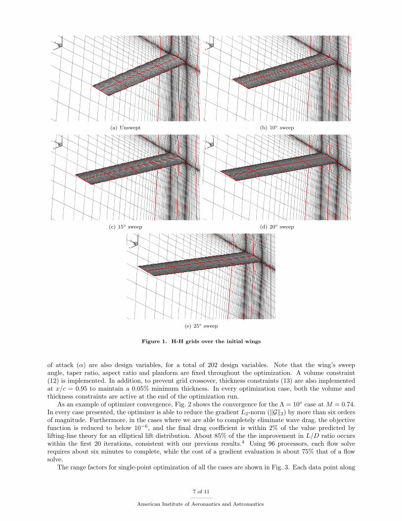
We perform single-point drag minimization on untapered wings at transonic speeds between M = 0.60 andM = 0.86. Each optimization is performed at a fixed Mach number. Once the optimization has converged,the range factor R is computed for each optimized wing. The initial geometries are untapered wings withsweeps angles ranging from 0 to 25. The sweep angles of the wings are fixed during optimization. All thewings have the section geometry of the NACA 0012 airfoil, with an aspect ratio of A = 8.0. The volumegrids are 96-block H-H topology grids with 2.77-million nodes. The surface grids are shown in Fig. 1. Off-wallspacing is 2.0× 10−3c, and far-field boundaries are at least 22c from any point on the wing surface.

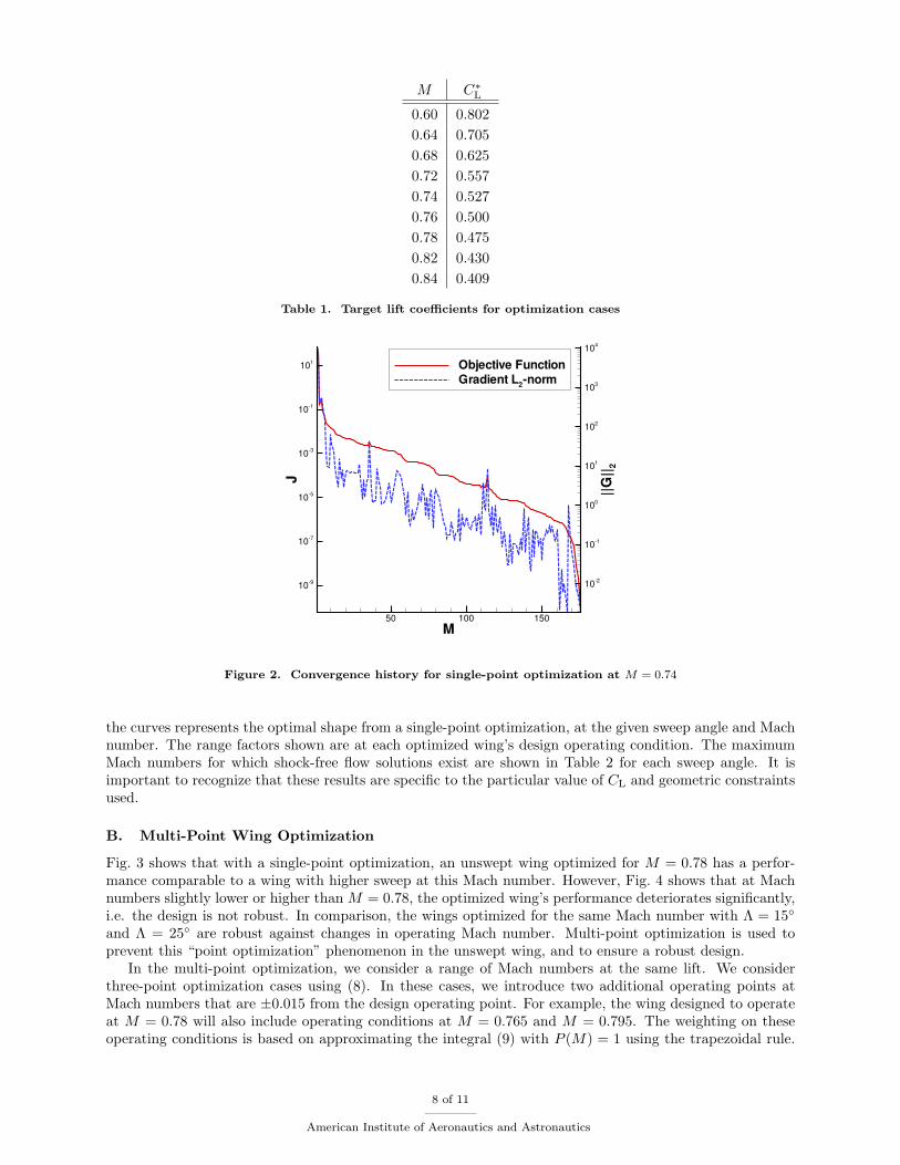
Our goal is to maximize the lift-to-drag ratio of this wing, while maintaining the same lift at eachoperating Mach number. That is, target C∗L is set such that M2C∗L is constant. The target lift coefficientsC∗L are shown in Table 1. A constant drag coefficient of CD0 = 0.0150 is added to the computed CD as anestimate of viscous effects and fuselage and engine interaction.2

The top and bottom surfaces of each wing are parameterized with a cubic B-spline surface with 13control points in the spanwise direction and 11 in the chordwise direction. There are 200 B-spline controlpoint design variables, which include z-coordinates of every control point, except near the leading edge andat the trailing edge, where the control points are fixed. The change in the twist angle (Ω) and the angle

6 of 11


X

Y

Z

(a) Unswept

X

Y

Z

(b) 10 sweep

X

Y

Z

(c) 15 sweep

X

Y

Z

(d) 20 sweep

X

Y

Z

(e) 25 sweep

Figure 1. H-H grids over the initial wings

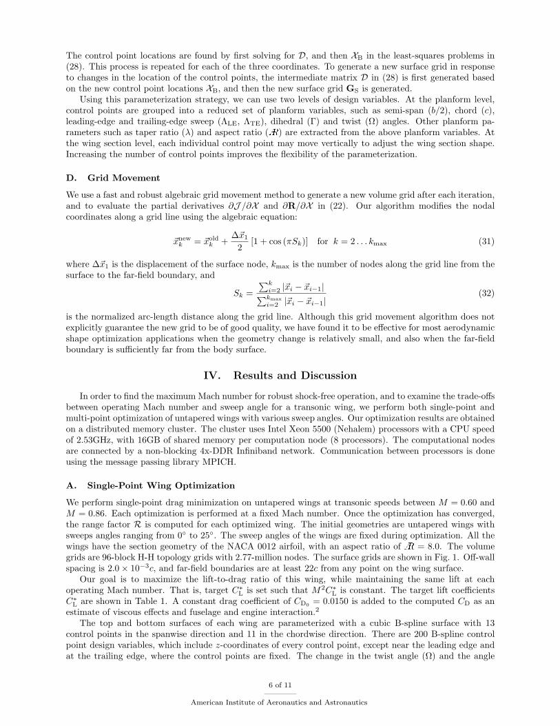
of attack (α) are also design variables, for a total of 202 design variables. Note that the wing’s sweepangle, taper ratio, aspect ratio and planform are fixed throughout the optimization. A volume constraint(12) is implemented. In addition, to prevent grid crossover, thickness constraints (13) are also implementedat x/c = 0.95 to maintain a 0.05% minimum thickness. In every optimization case, both the volume andthickness constraints are active at the end of the optimization run.

As an example of optimizer convergence, Fig. 2 shows the convergence for the Λ = 10 case at M = 0.74.In every case presented, the optimizer is able to reduce the gradient L2-norm (‖G‖2) by more than six ordersof magnitude. Furthermore, in the cases where we are able to completely eliminate wave drag, the objectivefunction is reduced to below 10−6, and the final drag coefficient is within 2% of the value predicted bylifting-line theory for an elliptical lift distribution. About 85% of the the improvement in L/D ratio occurswithin the first 20 iterations, consistent with our previous results.4 Using 96 processors, each flow solverequires about six minutes to complete, while the cost of a gradient evaluation is about 75% that of a flowsolve.

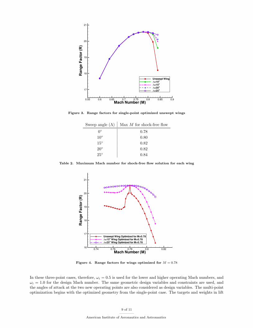
The range factors for single-point optimization of all the cases are shown in Fig. 3. Each data point along

7 of 11


M C∗L

0.60 0.8020.64 0.7050.68 0.6250.72 0.5570.74 0.5270.76 0.5000.78 0.4750.82 0.4300.84 0.409

Table 1. Target lift coefficients for optimization cases

M

J

||G||2

50 100 150

109

107

105

103

101

101

102

101

100

101

102

103

104

Objective Function

Gradient L2norm

Figure 2. Convergence history for single-point optimization at M = 0.74

the curves represents the optimal shape from a single-point optimization, at the given sweep angle and Machnumber. The range factors shown are at each optimized wing’s design operating condition. The maximumMach numbers for which shock-free flow solutions exist are shown in Table 2 for each sweep angle. It isimportant to recognize that these results are specific to the particular value of CL and geometric constraintsused.

B. Multi-Point Wing Optimization

Fig. 3 shows that with a single-point optimization, an unswept wing optimized for M = 0.78 has a perfor-mance comparable to a wing with higher sweep at this Mach number. However, Fig. 4 shows that at Machnumbers slightly lower or higher than M = 0.78, the optimized wing’s performance deteriorates significantly,i.e. the design is not robust. In comparison, the wings optimized for the same Mach number with Λ = 15

and Λ = 25 are robust against changes in operating Mach number. Multi-point optimization is used toprevent this “point optimization” phenomenon in the unswept wing, and to ensure a robust design.

In the multi-point optimization, we consider a range of Mach numbers at the same lift. We considerthree-point optimization cases using (8). In these cases, we introduce two additional operating points atMach numbers that are ±0.015 from the design operating point. For example, the wing designed to operateat M = 0.78 will also include operating conditions at M = 0.765 and M = 0.795. The weighting on theseoperating conditions is based on approximating the integral (9) with P (M) = 1 using the trapezoidal rule.

8 of 11


Mach Number (M)

RangeFactor(R)

0.55 0.6 0.65 0.7 0.75 0.8 0.85 0.9

17

18

19

20

21

Unswept Wing

Λ=10o

Λ=15o

Λ=20o

Λ=25o

Figure 3. Range factors for single-point optimized unswept wings

Sweep angle (Λ) Max M for shock-free flow

0 0.7810 0.8015 0.8220 0.8225 0.84

Table 2. Maximum Mach number for shock-free flow solution for each wing

Mach Number (M)

RangeFactor(R)

0.74 0.76 0.78 0.8 0.8216

17

18

19

20

21

Unswept Wing Optimized for M=0.78

Λ=15oWing Optimized for M=0.78

Λ=25oWing Optimized for M=0.78

Figure 4. Range factors for wings optimized for M = 0.78

In these three-point cases, therefore, ωi = 0.5 is used for the lower and higher operating Mach numbers, andωi = 1.0 for the design Mach number. The same geometric design variables and constraints are used, andthe angles of attack at the two new operating points are also considered as design variables. The multi-pointoptimization begins with the optimized geometry from the single-point case. The targets and weights in lift

9 of 11


Mach Number (M)

RangeFactor(R)

0.55 0.6 0.65 0.7 0.75 0.8 0.85 0.917

18

19

20

21

Unswept Wing

Λ=10o

Λ=15o

Λ=20o

Λ=25o

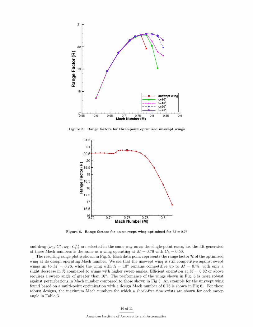
Figure 5. Range factors for three-point optimized unswept wings

Mach Number (M)

RangeFactor(R)

0.72 0.74 0.76 0.78 0.816

16.5

17

17.5

18

18.5

19

19.5

20

20.5

21

21.5

Figure 6. Range factors for an unswept wing optimized for M = 0.76

and drag (ωL, C∗L, ωD, C∗D) are selected in the same way as as the single-point cases, i.e. the lift generatedat these Mach numbers is the same as a wing operating at M = 0.76 with CL = 0.50.

The resulting range plot is shown in Fig. 5. Each data point represents the range factorR of the optimizedwing at its design operating Mach number. We see that the unswept wing is still competitive against sweptwings up to M = 0.76, while the wing with Λ = 10 remains competitive up to M = 0.78, with only aslight decrease in R compared to wings with higher sweep angles. Efficient operation at M = 0.82 or aboverequires a sweep angle of greater than 10. The performance of the wings shown in Fig. 5 is more robustagainst perturbations in Mach number compared to those shown in Fig 3. An example for the unswept wingfound based on a multi-point optimization with a design Mach number of 0.76 is shown in Fig 6. For theserobust designs, the maximum Mach numbers for which a shock-free flow exists are shown for each sweepangle in Table 3.

10 of 11


Sweep angle (Λ) Max M for shock-free flow

0 0.7610 0.7815 0.7820 0.8225 0.84

Table 3. Maximum Mach number for shock-free flow and robust design at each sweep angle

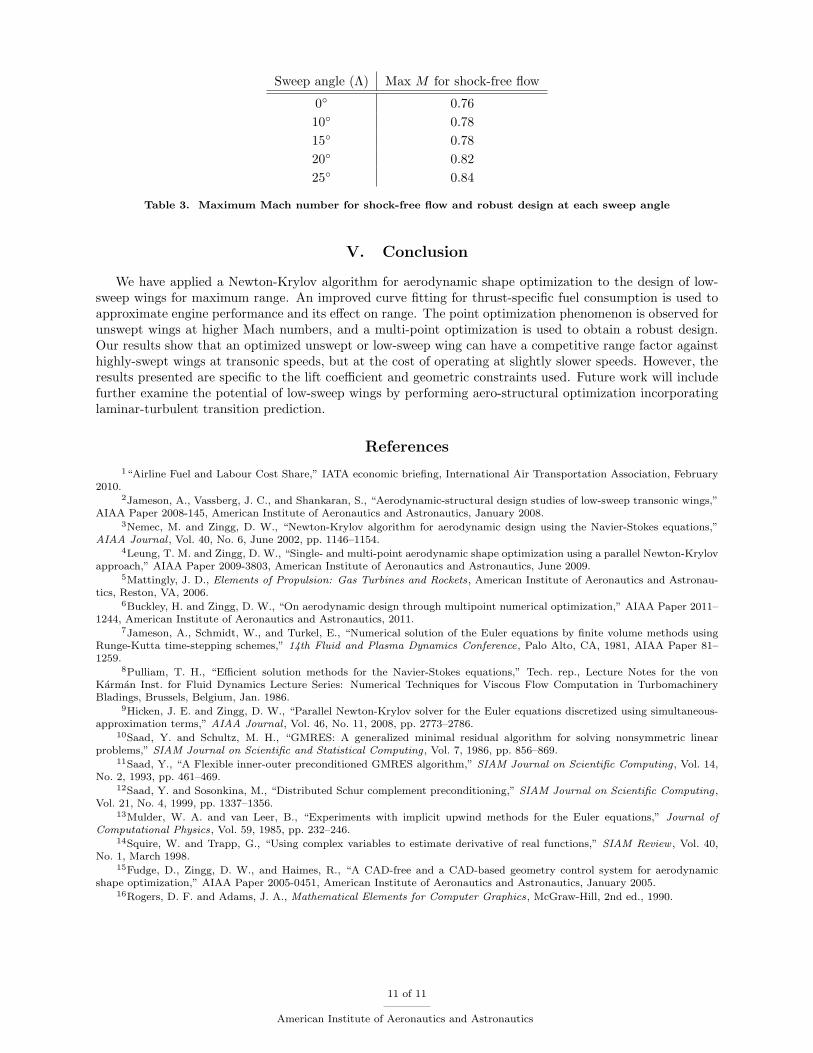
V. Conclusion

We have applied a Newton-Krylov algorithm for aerodynamic shape optimization to the design of low-sweep wings for maximum range. An improved curve fitting for thrust-specific fuel consumption is used toapproximate engine performance and its effect on range. The point optimization phenomenon is observed forunswept wings at higher Mach numbers, and a multi-point optimization is used to obtain a robust design.Our results show that an optimized unswept or low-sweep wing can have a competitive range factor againsthighly-swept wings at transonic speeds, but at the cost of operating at slightly slower speeds. However, theresults presented are specific to the lift coefficient and geometric constraints used. Future work will includefurther examine the potential of low-sweep wings by performing aero-structural optimization incorporatinglaminar-turbulent transition prediction.

References

1“Airline Fuel and Labour Cost Share,” IATA economic briefing, International Air Transportation Association, February2010.

2Jameson, A., Vassberg, J. C., and Shankaran, S., “Aerodynamic-structural design studies of low-sweep transonic wings,”AIAA Paper 2008-145, American Institute of Aeronautics and Astronautics, January 2008.

3Nemec, M. and Zingg, D. W., “Newton-Krylov algorithm for aerodynamic design using the Navier-Stokes equations,”AIAA Journal , Vol. 40, No. 6, June 2002, pp. 1146–1154.

4Leung, T. M. and Zingg, D. W., “Single- and multi-point aerodynamic shape optimization using a parallel Newton-Krylovapproach,” AIAA Paper 2009-3803, American Institute of Aeronautics and Astronautics, June 2009.

5Mattingly, J. D., Elements of Propulsion: Gas Turbines and Rockets, American Institute of Aeronautics and Astronau-tics, Reston, VA, 2006.

6Buckley, H. and Zingg, D. W., “On aerodynamic design through multipoint numerical optimization,” AIAA Paper 2011–1244, American Institute of Aeronautics and Astronautics, 2011.

7Jameson, A., Schmidt, W., and Turkel, E., “Numerical solution of the Euler equations by finite volume methods usingRunge-Kutta time-stepping schemes,” 14th Fluid and Plasma Dynamics Conference, Palo Alto, CA, 1981, AIAA Paper 81–1259.

8Pulliam, T. H., “Efficient solution methods for the Navier-Stokes equations,” Tech. rep., Lecture Notes for the vonKarman Inst. for Fluid Dynamics Lecture Series: Numerical Techniques for Viscous Flow Computation in TurbomachineryBladings, Brussels, Belgium, Jan. 1986.

9Hicken, J. E. and Zingg, D. W., “Parallel Newton-Krylov solver for the Euler equations discretized using simultaneous-approximation terms,” AIAA Journal , Vol. 46, No. 11, 2008, pp. 2773–2786.

10Saad, Y. and Schultz, M. H., “GMRES: A generalized minimal residual algorithm for solving nonsymmetric linearproblems,” SIAM Journal on Scientific and Statistical Computing, Vol. 7, 1986, pp. 856–869.

11Saad, Y., “A Flexible inner-outer preconditioned GMRES algorithm,” SIAM Journal on Scientific Computing, Vol. 14,No. 2, 1993, pp. 461–469.

12Saad, Y. and Sosonkina, M., “Distributed Schur complement preconditioning,” SIAM Journal on Scientific Computing,Vol. 21, No. 4, 1999, pp. 1337–1356.

13Mulder, W. A. and van Leer, B., “Experiments with implicit upwind methods for the Euler equations,” Journal ofComputational Physics, Vol. 59, 1985, pp. 232–246.

14Squire, W. and Trapp, G., “Using complex variables to estimate derivative of real functions,” SIAM Review , Vol. 40,No. 1, March 1998.

15Fudge, D., Zingg, D. W., and Haimes, R., “A CAD-free and a CAD-based geometry control system for aerodynamicshape optimization,” AIAA Paper 2005-0451, American Institute of Aeronautics and Astronautics, January 2005.

16Rogers, D. F. and Adams, J. A., Mathematical Elements for Computer Graphics, McGraw-Hill, 2nd ed., 1990.

11 of 11


design of low-sweep wings for maximum...

Documents