design of intelligent cross-layer routing protocols … · design of intelligent cross-layer...
TRANSCRIPT

APPROVED FOR PUBLIC RELEASE; DISTRIBUTION UNLIMITED.
STINFO COPY
AIR FORCE RESEARCH LABORATORY INFORMATION DIRECTORATE
DESIGN OF INTELLIGENT CROSS-LAYER ROUTING PROTOCOLS
FOR AIRBORNE WIRELESS NETWORKS UNDER DYNAMIC
SPECTRUM ACCESS PARADIGM
SAN DIEGO STATE UNIVERSITY
MAY 2011
FINAL TECHNICAL REPORT
AFRL-RI-RS-TR-2011-093
ROME, NY 13441 UNITED STATES AIR FORCE AIR FORCE MATERIEL COMMAND

NOTICE AND SIGNATURE PAGE Using Government drawings, specifications, or other data included in this document for any purpose other than Government procurement does not in any way obligate the U.S. Government. The fact that the Government formulated or supplied the drawings, specifications, or other data does not license the holder or any other person or corporation; or convey any rights or permission to manufacture, use, or sell any patented invention that may relate to them. This report is the result of contracted fundamental research deemed exempt from public affairs security and policy review in accordance with SAF/AQR memorandum dated 10 Dec 08 and AFRL/CA policy clarification memorandum dated 16 Jan 09. This report is available to the general public, including foreign nationals. Copies may be obtained from the Defense Technical Information Center (DTIC) (http://www.dtic.mil). AFRL-RI-RS-TR-2011-093 HAS BEEN REVIEWED AND IS APPROVED FOR PUBLICATION IN ACCORDANCE WITH ASSIGNED DISTRIBUTION STATEMENT. FOR THE DIRECTOR: /s/ /s/ MICHAEL MEDLEY WARREN H. DEBANY JR., Technical Advisor Work Unit Manager Information Grid Division
Information Directorate
This report is published in the interest of scientific and technical information exchange, and its publication does not constitute the Government’s approval or disapproval of its ideas or findings.

REPORT DOCUMENTATION PAGE Form Approved
OMB No. 0704-0188 Public reporting burden for this collection of information is estimated to average 1 hour per response, including the time for reviewing instructions, searching data sources, gathering and maintaining the data needed, and completing and reviewing the collection of information. Send comments regarding this burden estimate or any other aspect of this collection of information, including suggestions for reducing this burden to Washington Headquarters Service, Directorate for Information Operations and Reports, 1215 Jefferson Davis Highway, Suite 1204, Arlington, VA 22202-4302, and to the Office of Management and Budget, Paperwork Reduction Project (0704-0188) Washington, DC 20503.
PLEASE DO NOT RETURN YOUR FORM TO THE ABOVE ADDRESS. 1. REPORT DATE (DD-MM-YYYY) May 2011
2. REPORT TYPE Final Technical Report
3. DATES COVERED (From - To) January 2008 – October 2010
4. TITLE AND SUBTITLE DESIGN OF INTELLIGENT CROSS-LAYER ROUTING PROTOCOLS FOR AIRBORNE WIRELESS NETWORKS UNDER DYNAMIC SPECTRUM ACCESS PARADIGM
5a. CONTRACT NUMBER FA8750-08-1-0078
5b. GRANT NUMBER N/A
5c. PROGRAM ELEMENT NUMBER 62702F
6. AUTHOR(S) Sunil Kumar
5d. PROJECT NUMBER AN08
5e. TASK NUMBER SD
5f. WORK UNIT NUMBER SK
7. PERFORMING ORGANIZATION NAME(S) AND ADDRESS(ES) San Diego State University Electrical and Computer Engineering Department San Diego, CA 92182-1309
8. PERFORMING ORGANIZATION REPORT NUMBER
9. SPONSORING/MONITORING AGENCY NAME(S) AND ADDRESS(ES) Air Force Research Laboratory/Information Directorate Rome Research Site/RIGF 525 Brooks Road Rome NY 13441
10. SPONSOR/MONITOR'S ACRONYM(S) AFRL/RI
11. SPONSORING/MONITORING AGENCY REPORT NUMBER AFRL-RI-RS-TR-2011-093
12. DISTRIBUTION AVAILABILITY STATEMENT Approved for Public Release; Distribution Unlimited. This report is the result of contracted fundamental research deemed exempt from public affairs security and policy review in accordance with SAF/AQR memorandum dated 10 Dec 08 and AFRL/CA policy clarification memorandum dated 16 Jan 09.
13. SUPPLEMENTARY NOTES
14. ABSTRACT: The airborne military assets need to share the time-sensitive battlefield information among themselves, exchange the information with the ground troops for situational awareness purpose, and transfer it to the remotely located command and control center. The challenge in airborne networks (AN) is to organize a low-delay, reliable, infrastructure-less wireless network in the presence of highly dynamic network topology, heterogeneous air assets, intermittent transmission links and dynamic spectrum allocation. The QoS-aware cross-layer protocols are key enablers in effectively deploying the airborne infrastructure. This report considers the problem of designing cross-layer protocols for robust video transmission in mobile wireless networks, such as AN and wireless ad hoc networks (MANET). The cross-layer protocols need to consider the QoS issues in an end-to-end fashion and collaboratively design protocols at different network layers. First, a real-time and H.264 compliant video packet priority assignment scheme is discussed for error-prone wireless links in this report which can be deployed during H.264 encoding process with very small additional computational overhead. This packet priority assignment is used in an unequal error protection scheme by using the prioritized forward error correcting codes at the physical layer. In this scheme, low FEC code rates are used for higher priority packets and vice versa. Additionally a priority-aware MAC layer fragmentation scheme is designed for video packets in bit-rate limited error-prone wireless links. Specifically, the optimal fragment size is derived for each priority level which achieves the maximum expected weighted goodput at different encoded video bit rates and slice sizes. Packet fragmentation scheme also uses slice discard in the buffer due to the channel bit rate constraints. Both the cross-layer schemes demonstrate that the use of packet priority achieves considerable PSNR gain in the presence of channel errors. The network topology changes rapidly in high-mobility MANET, which causes established routes to become unstable and links to break. To provide reliable routes, two techniques are used: multipath routing and path maintenance. The former is capable of finding multiple paths during route discovery phase, while the latter is used to detect link failures. A new cross-layer ad hoc multipath routing scheme, called as ‘Adaptive Multimetric-AOMDV (AM-AOMDV)’ is designed for CBR traffic in MANET. Its performance is compared with other AODV and AOMDV reactive routing schemes for a wide range of varying node speeds, connections and packet rates.
15. SUBJECT TERMS Airborne networks, cooperative communications, cognitive radios, hybrid automatic-repeat-request protocols, code-division channelization, cross-layer optimization.
16. SECURITY CLASSIFICATION OF: 17. LIMITATION OF ABSTRACT
UU
18. NUMBER OF PAGES
127
19a. NAME OF RESPONSIBLE PERSON
MICHAEL MEDLEY
a. REPORT
U b. ABSTRACT
U c. THIS PAGE
U 19b. TELEPHONE NUMBER (Include area code)
N/A
Standard Form 298 (Rev. 8-98) Prescribed by ANSI Std. Z39.

i
TABLE OF CONTENTS
LIST OF FIGURES…..…………..………………………………………………….………… iv
LIST OF TABLES..……………..…………………………………………………………...….vi
SUMMARY……………………..……………………………………………………..…………1
1.0 INTRODUCTION………......………………………………………………………...……..3
1.1 Motivation..…………….……………………………………………………………..….3
1.2 Objectives....…………….………………………………………………………………..6
1.3 Organization of Report...………………………………………………………………....7
2.0 BACKGROUND AND ASSUMPTIONS…………………………………………………8
2.1 Cross Layer Design of Wireless Protocols for Robust Multimedia Transmission….……8
2.2 Design of Multimedia Bitstream……..………..……………………………....………..10
2.3 Modeling the Impact of other Layers on Cross-Layer Protocols...……………………..12
2.4 Design of Cross-Layer Fragmentation Protocols…...………………………………. …13
2.5 Design of Cross-layer Routing Protocols...……………………………………………..14
3.0 REAL TIME SLICE PRIORITIZATION MODEL FOR H.264 AVC VIDEO…….…17
3.1 Introduction……………………………………..………………………………….........17
3.2 Method and Assumptions……...…………………………….………………………….18
3.2.1 Packet Loss Visibility Model……..…….………………………………………….19
3.2.2 Factors Affecting Visibility Model………………………………………………...20
3.2.3 Generalized Linear Model.…...…………..………………………………………..22
3.3 Application to Packet Prioritization……………………………………………………..28
3.4 Results and Discussions…………………………………………………………………29

ii
3.4.1 Performance of Slice Priority Assignment…….………………………………......29
3.4.2 UEP Performance………………………………….………………………………30
4.0 H.264 VIDEO QUALITY ENHANCEMENT THROUGH OPTIMAL PRIORITIZED
PACKET FRAGMENTATION……....................……………………………………………32
4.1 Introduction……………………………………………………………………………..32
4.2 Method and Assumptions: Proposed Cross-Layer Fragmentation Scheme…………….35
4.2.1 Proposed H.264 Slice and Video Packet Formation………………………………35
4.2.2 Slice Priority……………………………………………………………………….36
4.2.3 Problem Formulation for Determining Optimal Fragmentation…………………...37
4.3 Simulation Results and Discussion………………………………………………….......49
4.3.1 Baseline System Performance…………………… ……………………………….49
4.3.2 Priority-agnostic Fragmentation Performance……………………………….…….54
4.3.3 Priority-aware Fragmentation Performance………………………………….……59
4.4 Conclusion………………………………………………………………………………67
5.0 ADAPTIVE MULTI-METRIC AD HOC ON-DEMAND MULTIPATH DISTANCE
VECTOR ROUTING…………..………………………………………………………………69
5.1 Introduction.……………………………………………………………………………..69
5.2 Related Work……………………………………………………………………………71
5.3 Path Maintenance Schemes……………………………...………………………….......76
5.4 Method: Description of AM-AOMDV Routing Scheme……………………………….78
5.4.1 Multiple Routing Metrics..……………………...…………………………………78
5.4.2 Route Setup Stage……………………………….…………………………………79

iii
5.4.3 Data Transmission using Local Path Update ……………………………………80
5.4.4 Enhanced link Layer Failure Handling…………….………………………………81
5.4.5 Keep Alive Mechanism: Secondary Route Maintenance… ………………………81
5.5 Effectiveness of AODV, AOMDV and AM-AOMDV………………………………...82
5.6 Simulation Results and Discussions……………………………..…………………...…83
5.6.1 Simulation Setup……………………………………………….…………………..83
5.6.2 Performance Comparison by Varying Node Speed……………….……………….85
5.6.3 Performance Comparison by Varying Number of Connections……….…………..90
5.6.4 Performance Comparison by Varying Packet Size ……………………….…….…96
5.7 Conclusion……………………………………………………………………………..101
6.0 CONCLUSIONS AND FUTURE RESEARCH DIRECTIONS………………………102
6.1 Conclusions………………………………………………………………..…………..102
6.2 Contributions…...…………………………………………………………...…………103
6.3 Future Research and Recommendations………………………………………………103
7.0 REFERENCES…………………………………………………………………..……..…105
LIST OF ACRONYMS……………………………………………………………………….117

iv
LIST OF FIGURES
Figure 1 The cross-layer design in military networks……………………….………………..…10
Figure 2 Illustration of our system design …...………………………………………………….18
Figure 3 RR and Modified RR framework used for extracting parameters ……………………..20
Figure 4 Results of a Random Forest test performed on the Training Data……………………..27
Figure 5 Cross-Layer fragmentation approach…………………………………………………..36
Figure 6 Expected Goodput G vs. fragment size y at (a) R=960 Kbps and different pb and (b)
pb=5x10⁻⁵ and different R………………………………………………...…………………...……41
Figure 7 Slice data discarded per second……………………..………………………………….42
Figure 8 (a) Expected Goodput, and (b) Slice discard comparisons between priority-agnostic and
priority-aware fragmentation…………………………………………….………............... 47
Figure 9 (a) Expected Goodput, and (b) Slice discard comparisons between priority-agnostic and
priority-aware fragmentation…………………………………….…………………………48
Figure 10 Error-free average video PSNR at different slice sizes and bit rates for (a) Foreman
and (b) Silent CIF sequences…………………………..…………………………………...51
Figure 11 Average PSNR in baseline system for Foreman video sequence encoded at (a) 720
Kbps, (b) 960 Kbps, and (c) 1080 Kbps…………………………………….……………...53
Figure 12 Average PSNR achieved by priority-agnostic fragmentation for Foreman video
sequence encoded at (a) 720 Kbps, (b) 960 Kbps and (c) 1080 Kbps……..……………….56
Figure 13 Gains achieved by 150 byte slices over 900 byte slices in priority-agnostic
fragmentation for Foreman video sequence, in terms of (a) Expected received goodput, and
(b) Average PSNR…………….............................................................................................57

v
Figure 14 Average PSNR gain achieved by priority-agnostic fragmentation over baseline system
for Foreman video sequence encoded at (a) 720 Kbps, and (b) 960 Kbps……...……….....58
Figure 15 Proposed slice discard scheme. Here Ds represents the number of bytes to be
discarded……………………………………………………………………………………60
Figure 16 Average video PSNR for priority-aware fragmentation of Foreman video encoded at
(a) 720 Kbps, (b) 960 Kbps, and (c) 1080 Kbps……………………………………………62
Figure 17 11th frame of Foreman video sequence encoded at 720 Kbps and BER of 5x10⁻⁵ in (a)
Baseline system: PSNR=20.3dB, (b) Priority-agnostic fragmentation: PSNR=25.2dB, and
(c) Priority-aware fragmentation: PSNR=29.9dB………..………………………...............66
Figure 18 50th frame of Silent video sequence encoded at 720 Kbps and BER of 5x10⁻⁵ in (a)
Baseline system: PSNR=22dB, (b) Priority-agnostic fragmentation: PSNR=28.5dB and (c)
Priority-aware fragmentation: PSNR=33.3dB…………...…………………………………67
Figure 19 Performance of different routing schemes for varying node speeds: (a) throughput per
flow, (b) Average end-to-end latency, (c) Normalized routing load, and (d) Number of
RREQ’s per second………………………………………………………………………....88
Figure 20 Performance of different routing schemes for varying number of connections: (a)
throughput per flow, (b) Average end-to-end latency, (c) Normalized routing load, and (d)
Number of RREQ’s per second………………………………………………………….…95
Figure 21 Performance of different routing schemes for varying packet rates: (a) throughput per
flow, (b) Average end-to-end latency, (c) Normalized routing load, and (d) Number of
RREQ’s per second.………………………………………………………………………...98
vi
LIST OF TABLES
Table 1 Regression Coefficients obtained from GLM Model…………………………………...28
Table 2 Percentage of Misclassifications using Fixed Slice Distribution………………………..30
Table 3 PSNR Performance of the UEP Scheme………………………………………………...31
Table 4 PSNR Gains of Priority-aware over Priority-agnostic Fragmentation Scheme (Without
Slice Fragmentation) for Foreman Video at 960 Kbps (1080 Kbps).…………………........63
Table 5 PSNR Gains of Priority-aware over Priority-agnostic Fragmentation Scheme (Without
Slice Fragmentation) for Silent Video at 960 Kbps (1080 Kbps)…………………………..63
Table 6(a) PSNR Gain of Priority-aware over Priority-agnostic Fragmentation Scheme (With
Slice Fragmentation) for Foreman (Silent) Video at 720 Kbps…………………...………..64
Table 6(b) PSNR Gain of Priority-aware over Priority-agnostic Fragmentation Scheme (With
Slice Fragmentation) for Foreman (Silent) Video at 960 Kbps...…………………………..65
Table 6(c) PSNR Gain of Priority-aware over Priority-agnostic Fragmentation Scheme (With
Slice Fragmentation) for Foreman (Silent) Video at 1080 Kbps…………………...………65
Table 7 Simulation Parameters…………………………………………………………………..84

1
SUMMARY
The airborne military assets need to share the time-sensitive battlefield information among
themselves, exchange the information with the ground troops for situational awareness purpose,
and transfer it to the remotely located command and control center. The challenge in airborne
networks (AN) is to organize a low-delay, reliable, infrastructure-less wireless network in the
presence of highly dynamic network topology, heterogeneous air assets, intermittent
transmission links and dynamic spectrum allocation. The QoS-aware cross-layer protocols are
key enablers in effectively deploying the airborne infrastructure.
This report considers the problem of designing cross-layer protocols for robust video
transmission in mobile wireless networks, such as AN and wireless ad hoc networks (MANET).
The cross-layer protocols need to consider the QoS issues in an end-to-end fashion and
collaboratively design protocols at different network layers. First, a real-time and H.264
compliant video packet priority assignment scheme is discussed for error-prone wireless links in
this report which can be deployed during H.264 encoding process with very small additional
computational overhead. This packet priority assignment is used in an unequal error protection
scheme by using the prioritized forward error correcting codes at the physical layer. In this
scheme, low FEC code rates are used for higher priority packets and vice versa. Additionally a
priority-aware MAC layer fragmentation scheme is designed for video packets in bit-rate limited
error-prone wireless links. Specifically, the optimal fragment size is derived for each priority
level which achieves the maximum expected weighted goodput at different encoded video bit
rates and slice sizes. Packet fragmentation scheme also uses slice discard in the buffer due to the
channel bit rate constraints. Both the cross-layer schemes demonstrate that the use of packet
priority achieves considerable PSNR gain in the presence of channel errors.
The network topology changes rapidly in high-mobility MANET, which causes established
routes to become unstable and links to break. To provide reliable routes, two techniques are
used: multipath routing and path maintenance. The former is capable of finding multiple paths

2
during route discovery phase, while the latter is used to detect link failures. A new cross-layer ad
hoc multipath routing scheme, called as ‘Adaptive Multimetric-AOMDV (AM-AOMDV)’ is
designed for CBR traffic in MANET. Its performance is compared with other AODV and
AOMDV reactive routing schemes for a wide range of varying node speeds, connections and
packet rates.

3
1.0 INTRODUCTION
1.1 Motivation
The Airborne Wireless Network (AN) must support the diverse AF missions, platforms, and
communications transport needs of the future. The network will vary from a single aircraft
connected to a ground station to support voice or low speed data, to a constellation of hundreds
of aircrafts transporting high speed imagery and real-time collaborative voice and full motion
video. The target network must be capable of forming a topology that is matched to the
particular mission, platforms, and data transmission needs, with minimum pre-planning and
operator involvement [1]. The AN nodes should be capable of establishing connections with
other AN nodes, whether airborne, in space, or on the surface, as needed. These links could be
asymmetric with respect to bandwidth, and may be bidirectional or unidirectional (including
receive only). Also, the forward and reverse network connections relative to any node could take
different physical paths through the network [1].
The AN connections may be point-to-point, broadcast, or multipoint/multicast. These
connections could be used to relay (receive and transmit with the same data formats and on the
same media/frequency), translate (receive and transmit with the same data formats but on
different media or frequencies), or gateway (receive and transmit with different data formats and
on different media/frequencies) the information, as needed. The connections could be established
either based upon a prearranged network topology, or autonomously without prearrangements,

4
and dynamically as opportunities and needs arise. Key inter-node connectivity functions include
the backbone connectivity, subnet connectivity and network access connectivity [1].
According to the ‘Airborne Network Architecture’ document by the USAF Airborne
Network Special Interest Group, the AN must deliver a set of routing protocols that can be run
on all platforms [1]. According to this document, the AN nodes must be capable of routing the
data packets to/from any local area network (LAN), subnet, backbone, or space or terrestrial IP
network as opportunities and needs arise. The AN routers/switches must also be capable of
performing static, dynamic or ad hoc routing as needed, with highly-dynamic flat or hierarchical
topologies. The AN should enable platforms to dynamically change their points of attachment to
the network with no disruption to traffic flows and minimal loss of data (i.e., seamless roaming),
in the presence of varying numbers of fast moving platforms at Mach speeds.
The following Routing Metric would guide the design of suitable routing scheme(s) [1]:
number of hops, bandwidth, delay and jitter, error link characteristics, relative reliability and
stability of each available path, traffic load, media preference (to prioritize non-performance
functions such as LPI/LPD, AJ, fast handoff capability), speed and direction of movement of the
platforms, and energy efficiency. Any combination of these route selection criteria could be used
for routing decisions, prioritized and weighted according to the user quality of service (QoS) and
class of service (CoS) needs, and mission requirements. Furthermore, the AN routing should be
capable of routing user information as unicast, broadcast, multicast, and anycast network
transmissions between AN nodes on any part of the AN or global information grid (GIG) [1].
The main objective of QoS-based routing in AN is the dynamic determination of feasible
paths while considering the highly dynamic topology, policy constraints, mission requirements,

5
disparate platforms and traffic patterns. The routes should be changed in response to changes in
the available communications resources, offered traffic patterns, and performance demands in
order to make the most efficient use of the network resources, in accordance with the
communications policy in place at the time. The QoS/CoS mechanisms must support all
communications services (e.g., voice, data, video), provide preferential treatment based on
priority, enable policy-based assignment of service classes and priorities, rapidly respond to
changes in assignments, and work end-to-end on all host and network devices, as needed [1, 13].
Analysis and shortcomings of the widely used routing schemes DSDV, DSR, DD, OLSR,
GPSR, and multi-path routing and their various extensions [9-20], was provided in ‘Airborne
Network Architecture’ document [1]. This document called for the need to develop highly
flexible cross-layer routing schemes for ANs.
We believe that the QoS-aware cross-layer protocols are key enablers in effectively
deploying the airborne infrastructure. The airborne military assets (such as UAVs, surveillance
and fighter aircrafts, and satellites) need to (i) share the time-sensitive information (such as
battlefield surveillance data/voice/image/video, ally pilots’ voice/data, command and control
information) among themselves, (ii) exchange the information with the ground troops for
situational awareness purpose, and (iii) transfer it to the remotely located command and control
center. The challenge in AN is to organize a low-delay, reliable, infrastructure-less wireless
network in the presence of highly dynamic network topology (due to very high flying speeds),
heterogeneous air assets, intermittent transmission links and dynamic spectrum allocation [1].
Therefore, we propose to carry out research in developing robust and QoS-aware cross-layer
routing protocols for DSANs that are closely integrated with the physical, data link and

6
application layers. For example, we shall investigate schemes which would consider (i)
collaborative spectrum sensing and channel management, (ii) spectrum mobility and handoffs
(due to user mobility) effects on spectrum sensing, channel access, link quality and routing/re-
routing delays; and (iii) application QoS (CBR/VBR, flow priority, desired latency, bit-rates,
flow duration, loss sensitivity) and user QoS (frame rate, frame size, packet priority, packet
scope) demands. Similarly, parameters from the physical layer (such as detected new spectrum
bands, interference temperature, radio fading characteristics, etc.) and the MAC layer (such as bit
error rate) could be utilized to self-adjust the route discovery.
1.2 Objectives
This report considers the problem of designing cross-layer protocols for robust video
transmission in mobile wireless networks, such as MANET and AN. The cross-layer protocols
need to consider the QoS issues in an end-to-end fashion and collaboratively design protocols at
different network layers. The objectives of this report are:
i. To design robust H.264 AVC video bitstream for error-prone wireless networks,
including the video packet formation, real-time packet priority assignments, partial
packet decoding.
ii. To show the importance of real time packet priority assignment for improving QoS in
cross-layer protocol design.
iii. To study the efficacy of a priority-aware MAC layer fragmentation schemes for video
data.

7
iv. To investigate the performance of ad hoc multipath routing schemes for CBR traffic in
MANET.
1.3 Organization of Report
Section 1 provides the motivation for this effort. Section 2 introduces the background and
assumptions of the techniques presented in this report, including the issues in cross layer design
of wireless network protocols, impact of other layers on these protocols, and need for designing
multimedia bitstream.
In Section 3, the video packet formation and a real-time packet priority assignment scheme
is designed for the state-of-the-art H.264 AVC video compression standard. The performance of
this scheme is compared with the full reference cumulative mean squared error (CMSE) based
scheme. A MAC layer H.264 video packet fragmentation for error-prone wireless channels is
discussed in Section 4. The performance of this scheme is compared with and without the use of
video packet priorities. In Section 5, a new adaptive multi-metric ad hoc on-demand multipath
distance vector (AM-AOMDV) routing scheme is presented. Its performance is compared with
other AODV and AOMDV schemes. In Section 6, the conclusions, report contributions, future
research and recommendation are presented.

8
2.0 BACKGROUND AND ASSUMPTIONS
The Air Force (AF) Wireless Networks (denoted as military networks in this report) must be
capable of supporting the diverse AF missions, platforms, and communications transport needs
of the future. The network may contain a constellation of hundreds of aircrafts and UAVs
transporting high speed imagery and real-time collaborative voice and video. The target network
should form a topology that is matched to the particular missions, platforms, and data
transmission needs, with minimum pre-planning and operator involvement [1]. The wireless
nodes should be capable of establishing connections with other node(s), whether airborne, in
space, or on the surface, as needed. These links could be asymmetric with respect to bandwidth,
and may be bidirectional or unidirectional (including receive only). Also, the forward and
reverse network connections relative to any node could take different physical paths through the
network [1].
2.1 Cross Layer Design of Wireless Network Protocols for Robust Multimedia
Transmission
The robust multimedia representation and QoS-aware cross-layer network protocols are key
enablers in effectively deploying the military network infrastructure. The military assets (such as
UAVs, surveillance and fighter aircrafts, satellites, ground units) need to (i) share the time-
sensitive information (such as battlefield surveillance data/voice/image/video, ally pilots’
voice/data, and command and control information) among themselves for situational awareness
purpose, and (ii) transfer it to the remotely located command and control center. The challenge in

9
military networks is to organize a low-delay, reliable, infrastructure-less wireless network in the
presence of highly dynamic network topology (due to very high flying speeds), heterogeneous air
assets, intermittent transmission links and dynamic spectrum allocation [1].
The robust and QoS-aware cross-layer network protocols for military networks should be
closely integrated with the physical, data link and application layers as shown in Figure 1.
Specifically these protocols should consider the application QoS (CBR/VBR, flow priority,
desired latency, bit-rates, flow duration, loss sensitivity) and user QoS (frame rate, frame size,
packet priority, and packet scope) demands. Similarly, parameters from the physical layer (such
as radio fading characteristics, modulation, forward error correction (FEC) and effective channel
capacity, etc.) and the MAC layer (such as bit error rate) could be utilized to self-adjust the
protocol operations.

Figure 1: The cross layer design in military networks.
2.2 Design of Robust Multimedia Bitstream
Live imagery and video streaming plays a critical role in situational awareness in tactical
operating environments. The military net-centric environment consists of heterogeneous nodes
(such as ground troops, airborne and space assets), which form highly dynamic wireless networks
characterized by different node speeds, node density, energy resources, available spectral bands,
link capacities and channel error rates. Military video applications also demand real-time (or
near-real-time) transmission of the data for entire application duration. But the ad-hoc and highly
dynamic nature of tactical wireless networks poses unique challenges to video transmission not
encountered in commercial networks. Moreover, the compressed video data delivery is very
susceptible to the packet losses and not all the bits and video packets are created equal. For
10

11
instance, loss of even a few important video data packets can lead of the loss of large number of
video frames, which may not be retransmitted entirely in delay sensitive applications (e.g.,
tactical targeting or in-theater operations).
The video data should therefore be intelligently compressed and packetized in a scalable and
robust manner, especially suited to the diverse military network characteristics and application
requirements (e.g., bit rates, tolerable delay, and mission types). This demands the integrated
design of: (i) next generation of ‘network-friendly’ video bitstream and packetization schemes to
deliver the improved video quality on disadvantaged radio links; (ii) scalable physical layer
techniques (i.e., adaptive hierarchical modulation and prioritized forward error correction codes)
for providing unequal error protection (UEP) for prioritized bit streams; (iii) a new quality-of-
service (QoS)-aware video rate control, packet scheduling, transport, routing and fragmentation
protocols that are cognizant of both network side information (i.e., parameter abstraction from
application and network layers) and the channel side information.
While the need for cross-layer adaptivity has been recognized in the literature, the art of
video streaming over ad hoc networks is still in its infancy, especially when addressed via a
cross-layer network design framework. Most of the recent research [2-5] only considers a subset
of layers of the protocol stack for rate-distortion optimization over quasi stationary channels.
Much work still needs to be done along these directions to identify and exploit cross-layer
interactions in real-time video streaming for tactical ad-hoc wireless networks.
In order to ensure graceful degradation of the decoded video quality in the presence of losses,
a scalable video coding scheme with error resiliency is desired. This allows for simple adaptation
to network (in terms of available bandwidth, link capacity fluctuations or error conditions) and
12
terminal (in terms of frame rate and picture size) capabilities. For instance, the network
abstraction layer (NAL) of the state-of-art H.264 AVC video codec enables the packetization and
transportation of compressed video bitstream over a wide range of networks. However, at present
the H.264 video compression standard cannot simultaneously achieve both strong error resiliency
and scalability features in a unified framework, and this represents an area of active research in
academia and industry. Moreover, these efforts do not consider the unique requirements for
military applications.
2.3 Modeling the Impact of other Layers on Cross-Layer Protocols
The protocols must consider the close interaction among different layers, beginning with
PHY as discussed below:
• Application-level QoS parameters such as source data rates, latency (real-time vs. non-
real-time), loss sensitivity, constant bit-rate vs. variable bit-rate. For this one should
consider the characteristics of compressed H.264 AVC video bitstreams in terms of their
scalability (frame-rate, frame-size, fine granularity scalability), error resiliency (data
partitioning, resynchronization, interleaving, etc.), packetization, metadata, packet scope,
packet priority, etc. [6-8].
• Network-level QoS parameters such as available bandwidth, link BER and packet loss
rates, flow priority [6-7]. Please note that the values of these parameters will considerably
vary due to the spectrum mobility and dynamic topologies.
• Effect of PHY including the spectrum sensing delays and spectrum mobility. Each
channel could suffer from varying interference levels and noise. The modulation (BPSK,

13
QPSK, etc.) and code rates (1/2, 1/3, etc.) also depend on channel conditions and required
QoS. Another important aspect is the channel heterogeneity as different channels may by
located on widely separated slices of frequency spectrum with different bandwidths and
different propagation characteristics [9-12].
• Effect of data link layer: presence of common channel signaling, scheduling, channel
access delays, connection establishment and management policies to adapt to spectrum
mobility and sharing. Similarly, the choice of CDMA vs. OFDM and the effect of
Doppler on multiplexing schemes [12].
Since there are too many parameters, many of them inter-dependent, a small set of
metrics could be used to consider the cost of a configuration for the protocol layer. For
example, one possibility is to measure the cost of configurations as some weighted combination
of data rate, transmission delay, error rates, etc.
2.4 Design of Cross-Layer Rate Control, Packet Scheduling and Fragmentation Protocols
The QoS-aware Rate Control, Packet Scheduling, and Data Fragmentation schemes are
essential for reliable video transmission over wireless ad hoc networks. However, the existing
schemes do not simultaneously consider the characteristics of video bitstreams (such as packet
priority, choice of scalability, etc.), network (such as congestion and collision), PHY (such as
channel error rates, available bandwidth, choice of hierarchical modulation) and the end-user
QoS requirements in a cross-layer fashion. As a consequence, these schemes fail to provide the
end-to-end rate control for reliable transmission of prioritized packets whose loss would cause
significant fluctuations in the video signal quality.

14
Video priority-aware rate control, scheduling and fragmentation schemes based on the video
bitstream, network and PHY characteristics are likely to provide better performance. Selective
packet rescheduling/retransmission could be applied for high priority packets. The encoder can
use more powerful FEC schemes (i.e., rate of the channel codes is adapted according to the
packet priority) or switch to a different frequency or channel. As a result, the FEC codes rates
and fragmentation sizes should be jointly optimized for prioritized video bitstream and the effect
of NALU size should be studied on the received video quality for various channel losses. The
network simulation tool (ns-2) can be used to simulate a multi-user and multi-hop wireless ad
hoc network. Performance metrics of interest include the received video quality (PSNR and
VQM) for a specified bit-rate, buffer size as well as the channel and congestion-induced packet
losses.
2.5 Design of Cross-layer Routing Protocols
The military nodes must be capable of routing the data packets to/from any local LAN,
subnet, backbone, or space or terrestrial IP network as opportunities and needs arise. The
routers/switches must also be capable of performing static, dynamic or ad hoc routing as needed,
with highly-dynamic flat or hierarchical topologies.
The main objective of QoS-based routing in military networks is the dynamic determination
of feasible paths while considering the highly dynamic topology, policy constraints, mission
requirements, disparate platforms and traffic patterns. The routes should be changed in response
to changes in the available communications resources, offered traffic patterns, and performance
demands in order to make the most efficient use of the network resources, in accordance with the

15
communications policy in place at the time. The QoS/CoS mechanisms must support all
communications services (e.g., voice, data, video), provide preferential treatment based on
priority, enable policy-based assignment of service classes and priorities, rapidly respond to
changes in assignments, and work end-to-end on all host and network devices, as needed [1, 13].
Analysis and shortcomings of the widely used routing schemes, including AODV, DSDV, DSR,
DD, OLSR, GPSR, and multi-path routing and their various extensions [14-23], has been
provided in [1].
The following Routing Metric would guide the design of suitable routing scheme(s) [1]:
number of hops, bandwidth, delay and jitter, link error characteristics, relative reliability and
stability of each available path, traffic load, media preference (to prioritize non-performance
functions such as LPI/LPD, AJ, fast handoff capability), speed and direction of movement of the
platforms, and energy efficiency. Any combination of these route selection criteria could be used
for routing decisions, prioritized and weighted according to the user quality of service (QoS) and
class of service (CoS) needs, and mission requirements. Furthermore, the routing should be
capable of routing user information as unicast, broadcast, multicast, and anycast network
transmissions between nodes on any part of the network or GIG [1].
Since military network environment has complex and dynamic architecture, and demands
complex service functions, no single wireless mobile routing protocol can fit all the needs [1,
13]. Therefore, the routing protocol should be designed as a combination of smaller building
blocks, namely, routing components. By analyzing the basic routing components, their
interaction and different technical approaches for each component, one can design a more
adaptable, flexible, robust, scalable and extendible component-based routing (CBR) protocol [24,

16
25]. In CBR, one can tailor routing behaviors to different application profiles and time varying
environment parameters at a reasonable cost. It would also be easier to extend CBR to integrate
with other protocol layers, accommodate new services or support new features.

17
3.0 REAL TIME SLICE PRIORITIZATION MODEL FOR H.264 VIDEO
3.1 Introduction
H.264 AVC is a state-of-the-art video coding standard developed by the ITU/ISO Joint Video
Team (JVT). Its enhanced compression performance and “network friendliness” makes this
standard very popular. The Video Coding Layer (VCL) in H.264 generates the coded
macroblocks (MB) [8, 26]. These MBs are aggregated to form slices at the Network Abstraction
Layer (NAL) by exploiting Context Adaptive Coding. Each slice is appended with a 1-byte
header. These slices are then transmitted over wireless network. However, the compressed video
data is very susceptible to channel errors. Therefore, it is important to prioritize video slices so
that high priority slices can be transmitted with greater protection and reliability in unreliable
channel conditions. This helps to maintain a certain level of perceptual video quality.
H.264 slices contribute different levels of video quality degradation due to channel errors. By
developing a deeper understanding of slices loss visibility for real time systems over wireless
networks, we can protect and transmit high priority slices over error-prone channels. Some slice
losses last a single frame while others last till the end of group of pictures (GOP). Consequently,
we consider the problem of predicting the packet loss visibility for real time systems using
Cumulative Mean Square Error (CMSE) as a metric to evaluate the video quality. Though we use
CMSE, our model can be extended to consider other quality metrics. However, CMSE is a
computationally intensive and time consuming process as all the frames in the GOP have to be
decoded and their Mean Square Error (MSE) summed. This introduces delay at the receiver. As a
result, computing CMSE is not a feasible approach for systems with latency constraints. In this

section, we discuss a new method for predicting the distortion introduced by the slice loss by
using the Generalized Linear Model (GLM). GLM can predict the expected value of CSME by
considering different video characteristics and various other attributes at the location of the loss.
In the next section, we give a brief overview of the system design. Following this we discuss
the concept of packet loss visibility model and explain how GLM can be used to model the
impact of a slice loss on the video quality.
3.2 Method and Assumptions
The Figure 2 below illustrates the proposed method to predict CMSE using GLM.
Figure 2: Illustration of our system design.
During compression, video parameters, such as motion vectors and residual energy, are
extracted as shown in the Parameter Extraction block. For model development, CMSE is
computed as shown in the Distortion Module by considering the loss of one slice at a time.
18

19
Following this, the model is developed in the Data Modeling section. We consider a wide range
of videos and encoding configurations, including variations in target bitrates, NAL sizes, and
video sequences of varied motion information, which will be described later. Once the model is
built, slice priority is estimated based on the predicted CMSE values.
3.2.1 Packet Loss Visibility Model
Our objective is to develop a packet loss visibility model for real time systems. Due to delay
constraints in streaming applications, we must only consider video features that can be extracted
while the MBs of a frame are being encoded, without using the future frames. This limits the
number of parameters that would be available to us for modeling. Therefore, we do not consider
the Full Reference model (FR-model), where parameters can be extracted from any point in the
communications system [27]. Please note that an FR model has access to parameters extracted
from the compressed, reconstructed and decoded videos, which represent a more complete set of
video characteristics for data modeling. Figure 3 shows a modified Reduced Reference model
(RR-model) used in our approach. In this model we access the compressed and reconstructed
video while the parameters are being extracted but not the decoded video at the receiver. As a
result, the residual (actual CMSE – predicted CMSE) would remain larger when compared to the
FR-model. However, we propose to overcome this loss of accuracy by prioritizing the video
intelligently and by using smart slice discard schemes, such that good perceptual video quality
can be maintained at the receiver.
It is important to note that that our model predicts CMSE that would occur in the event of a
slice (or packet) loss. Therefore, our model will help us to monitor quality as the video packets
enter the network. Consequently, we can use our packet loss visibility model to assign priorities

to the packets before they are transmitted over the network. The assigned priorities give an
indication of the impact of losing a specific packet on the received video quality.
20
Figure 3: RR and Modified RR framework used for extracting parameters.
3.2.2 Factors Affecting Visibility
In this section, we describe the video parameters that can be extracted easily while the MBs
are being encoded and the slices are being formed for modeling the packet loss visibility. An
approach similar to that shown in [28] has been adopted in our work. In order to create a
versatile model, we will examine the CMSE contributed by the packet loss, by considering the
error free reconstructed video frames and the error signal due to the packet loss.
Motion Related Parameters: Motion information is an important feature and is independent of
the compression algorithm. We assign each MB a single motion vector which is a weighted
average of the motion vectors in all the MB partitions. We define MOTX and MOTY to be the
mean motion vector in the x and y directions over all the MBs in slice. Other motion related
parameters are MOTPHASE, SigMean and SigVar. Here, MOTPHASE represents the phase of
Compressed Bitstream
Original Video
Encoder Compressed and Reconstructed Video
Extracted Parameters
Transmission Channel
Decoder
Decoded Video
RR Modified RR

21
motion vectors and only non-zero motion vectors are used. SigMean and SigVar are the mean
and variance of the signal.
Residual Energy represents the energy (sum of squares) of all coefficients of an MB’s residual
information after motion compensation. MAXRSENGY and AVGRSENGY represent the
maximum and average residual energy values of all the MBs in a slice.
Average Inter Parts: In H.264 AVC, each MB may be sub divided into partitions. Macroblocks
with more complex motion are encoded with more sub partitions. This helps preserve the
granularity of the motion information. AVGINTERPARTS represents the number of sub
partitions of all the MBs in a given slice.
Initial Mean Square Error (IMSE) represents the MSE between the error-free reconstructed
MB and the lossy concealed MB. Factors AVGIMSE and MAXIMSE are the average and
maximum IMSE of all the MBs in the slice. For the purpose of data modeling, we compute
CMSE as the sum of IMSE values from the inception of the slice loss till the end of GOP.
Frame Type and Location is a content independent factor. Location of the frame in a GOP
gives a measure of its propagation length or its temporal duration (TMDR), which represents
the maximum number of frames that may be affected by the slice loss. Since the loss of a slice in
initial frames of a GOP propagates longer, the contributed CMSE is likely to be greater than the
effects of slices loss from the later frames in a GOP. It should be noted that B-frames have a
propagation length of only 1 as they are not used as references frames.
Initial Structural Similarity Index (ISSIM) per MB is computed in the RR framework using
local means and variances of the encoded and decoded signals [29].

Other factors affecting the visibility of a slice loss include properties of scene changes,
concealment reference and camera motion. These attributes of the video are measured at the
Server and are not suited for real time systems.
3.2.3 Generalized Linear Model
The class of GLM is an extension of the classical linear models [30]. GLM is defined in
terms of a set of independent random variables Y1, Y2 ... YN, each with a distribution from the
exponential family. The distribution of each Yi has the same canonical form (e.g., all Normal or
Binomial, etc.). The vector of means µ constitutes the systematic part of the model and we
assume the existence of covariates x1, x2 … xp with known values such that:
(1)
Here β’s are parameters whose values are usually unknown and have to be estimated from the
data. If we let i be the index of the observations, the systematic part of the model can be written
as a function of the random part of the model as shown in below:
i= 1, …, N (2)
where xij is the value of jth covariate for observation i. This can be written more elegantly using
the matrix notation (where µ is n x 1, X is n x p and β is p x 1):
E(Y) = µ = Xβ, (3)
where ‘X’ is the model matrix and ‘β’ is the vector of parameters. In GLM, the systematic
component relates to the random component through a link function. The link function relates
22

the linear predictor η to the expected value µ of a datum y. The canonical link function for the
Normal family is the Identity, i.e. η = µ.
(4)
Given N observations, we can fit a model with up to N parameters. The simplest model is the null
model, which has the constant ϒ. Similarly, we can fit a Full model with as many factors as there
are observations. GLMs use an iteratively weighted least squares method to solve for the
regression coefficients (i.e., β vector).
For our modeling purposes, we collected data from various video sequences such as
Foreman, Bus, Coastguard, Stephan, Opening_Ceremony and Table_Tennis. The Foreman and
Bus sequences have CIF (352x288) resolution whereas the remaining sequences have 720x480
resolution. These sequences have 300, 150, 300, 300, 250 and 450 frames, in that order. The
encoding configuration spanned various bitrates from 256kbps to 1024kbps; to various fixed
NAL sizes of 150, 300, 450 and 600bytes. All the sequences were encoded at 30 frames per
second (fps). The GOP structure used is IDR B P... B IDR, with GOP length of 20 frames. The
reference software used was JM 14.2 [31] and the concealment used at the decoder was motion
copy. The data used to train our model captures different types of video sequences including the
low vs. high motion and low vs. high details, and wide range of coding configurations and spatial
resolutions, to ensure that our training set is not dominated by the effects of any single
configuration. In order to keep consistency of the model, we chose a 70-30% ratio to split our
data into training and test sets. The model is trained on the training set data and then tested using
the remaining data from our test set. Once our training and testing sets were formed, we
23

developed our model by performing parameter selection. The statistical software R [32] was used
for model fitting and analysis.
GLM Model Building
• Examine the response variable CMSE: We examined the CMSE distribution by plotting its
histogram. We observed that it follows an Inverse Gaussian Distribution. This is also an
intuitive result as CMSE cannot be negative (the system will have 0 CMSE when there are no
packet losses and the values of CMSE would vary depending on the location the frame
within GOP). However, due to the size of training set; with N >> p, where p is the number of
factors or parameters, the distribution of CMSE can be approximated to the Normal
distribution. The response variable distribution determines the family of the distribution for
GLM. Therefore, our datum belongs to the Gaussian family.
• Parameter selection: A step wise approach has been used to build the model. Akaike
Information Criterion (AIC) is used as the measure of the goodness of fit of the model. It
gives the relative measure of the information lost. In order to determine the best possible
model for a given set of data, the following stepwise process was followed:
o Step 1: Start with the Null model. Fit the Null model first.
o Step 2: Fit a univariate model for each parameter and compute the AIC value for each
univariate model. We get ‘p’ univariate models for p parameters. The AIC for each model
is computed as follows:
(5)
Where “L” is the likelihood, “edf” is the effective degree of freedom and “k” is the
multiple in the penalty.
24

25
o Step 3: From the set of univariate models formed in Step 2, choose the univariate model
with the lowest AIC value. The parameter from this chosen univariate model is selected
as the first parameter for our main effects model. For example, we found that IMSE was
the first parameter to be included in the main effects model.
o Step 4: Next, we construct p-1 models each of which has two parameters, by adding each
of the remaining p-1 parameters to the univariate model chosen from Step 3. AIC is
computed for these p-1 models and the model with the smallest AIC is chosen. At this
stage, our main effects model will have 2 parameters, i.e. IMSE and the 2nd parameter
chosen from the p-1 parameters.
o Step 5: Now we have 2 parameters in our main effects model and the p-2 remaining
parameters to choose from. At this stage, we construct a new set of p-2 intermediate
models, each of which has 3 parameters. The first two parameters are from Step 4 and the
3rd parameter is added, one parameter at a time, from the set of p-2 parameters. Again, the
model with the smallest AIC is chosen.
o Step 5 is repeated until the AIC is the lowest possible value for the given parameters.
With the addition of each parameter, the overall AIC would decrease indicating that the
loss in the entropy would also decrease. That is, by adding the parameters we are
reducing the amount of variation in the residue. This process is repeated until the best
possible model for our data is achieved.
Generally, the best way to identify the optimal number of parameters for a model is to
examine a plot of the AIC vs. number of parameters. The characteristic function of this plot takes
the form of a convex shaped curve and the optimal number of parameters is given by

26
determining its global minimum. However, this technique is not feasible in our model because
we have only a small number of parameters due to the real-time constraints. Therefore the global
minimum cannot be achieved.
We therefore, build the model and examine the AIC plot. We have used another statistical
tool (i.e., Random Forest) to examine the importance of parameters. The Random Forest is an
ensemble classifier that consists of many decision trees and outputs the class that is the mode of
the class’s output by individual trees. This helps us identify the relative importance of parameters
which also helps us study the interactions between different parameters. We have constructed a
Random Forest with 1000 trees. The Figure 4 below illustrates the importance of the parameters.
It can be seen that IMSE is the most important parameter as it has the best correlation with
CMSE. The parameters are arranged in the decreasing order of importance by evaluating the
‘Node purity’ and ‘change in the residual’ which occurs when the trees are pruned. At each node
in the tree, the percentage of increase of the MSE (residue) contributed by a variable is
computed. Important variables will change the predictions significantly. Hence, there will be an
increase in the %IncMSE. Similarly, if the change in the residue can be explained by a
parameter, the impurity at that node due to that parameter will decrease. This implies that the
change in purity of a node will increase indicating the importance of that parameter. In our plots,
IMSE attributed the maximum change in the MSE at a node, followed by the parameters TMDR
and ISSIM. In the second plot (IncNodePurtity), we observe that the maximum purity of a node
is attributed by the presence of IMSE, followed by parameters TMDR and MAXRSENGY.
By introducing interactions between IMSE and TMDR, and IMSE and Residual Energy
parameters, the accuracy of our predictions increased. In order to limit the relative complexity of

the model, we chose not to include further interactions or parameters. Our final model is
summarized in Table 1. We observe that the CMSE increases with IMSE. It should also be noted
that increase in MOTY also reflects the increase in CMSE. This is due to the fact that an object
in a slice could exceed its dimensions in the next frame (i.e. the object can move out of the
frame), thereby making it difficult to conceal the object if that slice were to be lost. As a result an
increase in motion in the ‘y’ direction would result an increase in CMSE. Though it is easy to see
the direct correlation of IMSE with CMSE, it is more difficult to interpret the correlation of other
regression coefficients by just considering their sign. It should be noted that regression
coefficients of the final main effects model should be analyzed as a complete entity and
evaluating the coefficients individually with CMSE would not give the best interpretation of the
model, because the value of a regression coefficient is determined given that all the other
parameters were present in the main effects model.
Figure 4: Results of a Random Forest test performed on the Training Data.
27
27

28
Table 1: Regression Coefficients Obtained from GLM Model
PARAMETER REGRESSION COEFFICIENT
IMSE 1.288e-01
TMDR -1.138
MAXRSENGY -5.729e-10
ISSIM -9.337e1
SigMean -1.759e-01
SigVar -4.028e-04
Motx -2.542e-01
AvgInterParts -3.354
Slice_type -1.120
Moty 4.902e-01
3.3 Application to Packet Prioritization
Our GLM model can be used to predict CMSE contribution of a slice and assign priority to
individual slices at the output of the encoder. The following four schemes can be used to
prioritize the slices at the output of the encoder. The prioritized slices are then sent over a lossy
wireless channel with forward error correcting code applied to them.
Variable Slice Distribution: This prioritization scheme considers the distribution of predicted
CMSE values for every slice. The mean and modal values give a measure of the skewness of the
data, thereby facilitating higher precision priority assignment. If the mode of the predicted values
is greater than the mean, the slices with predicted CMSE higher than the mode are assigned
higher priority. Otherwise, the slices with predicted CMSE greater than the mean would have

29
higher priority. All the remaining slices are assigned lower priority. This scheme can be extended
to four priorities by medians of the distribution.
Fixed Slice Distribution: Each frame is split into four priorities each with 25% of the slices
arranged in descending order of their predicted CMSE.
Variable Slice Distribution combined with Frame Type: All B-frame slices are assigned the
low priority and the variable slice distribution is applied for IDR, I and P frame slices.
Fixed Slice Distribution combined with Frame Type: All B-frame slices are assigned low
priority and the fixed slice distribution is applied for IDR, I and P frame slices.
3.4 Simulation Results and Discussions
In this section we first study the performance of our model with respect to CMSE, followed
by an unequal error protection (UEP) scheme by using the slice priorities assigned by this model.
3.4.1 Performance of Slice Priority Assignment
We test the performance of our model on Foreman sequence which has been encoded at
960kbps with a fixed slice size of 150 bytes. The model built in the above sections was used to
predict the CMSE values for the slices of this sequence and the resulting values were classified
into three priorities using the fixed slice distribution. The results are summarized in Table 2. We
have defined three levels of misclassification of the slices. Misclassification by Level 1 (or Level
2, Level 3) indicates that the priority assigned to the slice by our model has an error of one
priority class (or two priority classes, 3 priority classes) as compared to the priority assigned by
the CMSE. We observe that 56% slices were correctly classified and only 9.9% had a

30
classification error of 2 or more classes. This indicates that our GLM model predicts data with
sufficient accuracy.
Table 2: Percentage of Misclassifications using Fixed Slice Distribution
Degree of Misclassification % Slices
Level 1 36.0
Level 2 8.4
Level 3 1.5
3.4.2 UEP Performance
In order to minimize the effects of transmission errors on reconstructed video quality, we
have used the slice priorities assigned by this model to design an UEP scheme. The UEP is based
on the idea that more important video data should be given higher protection at the cost of less
important data. At the physical layer, UEP can be achieved by using FEC codes. The H.264
video packets with unequal levels of importance are protected by either the equal rate
convolutional codes or the prioritized Rate-Compatible Punctured Convolutional (RCPC) codes.
The RCPC codes achieve UEP by puncturing off different amounts of coded bits of the parent
code. The ordinary convolutional code to be punctured is called the parent code and the resulting
RCPC codes are called the children codes. Compared with the parent code, the RCPC codes are
of higher rates and give poorer BER performance but they can easily provide flexible choices of
code rates.
The H.264/AVC was used to encode the Foreman video at 780Kbps for 150 byte slice size.
The slices were assigned to three priority classes by using the GLM model described above. We

31
used a channel bit rate of 1080 Kbps with Rayleigh fading. Table 3 shows the channel signal-to-
noise ratios (CNR), average FEC code rate and RCPC code rates. In order to keep the output bit
rate constant for the non-prioritized (i.e., equal code rate) and RCPC code rates, we use the same
average code rates for both schemes. The excessive data after FEC protection is discarded from
the lowest priority slices. We observe that the prioritized FEC gives 0.9 to 2.5 dB PSNR
improvement over the equal code rate schemes. This demonstrates that our priority assignment
scheme indeed assigns priority effectively. Please note that the proposed scheme achieves lower
PSNR gain at 16dB and 18dB because the source rate is relatively high and applying lower
RCPC code rates results in considerable slice drops which degrades video quality.
Table 3: PSNR Performance of the UEP Scheme
Channel
CNR (dB)
Average FEC
Code Rate
RCPC Code
Rates
Non-Prioritized
RCPC Codes,
PSNR (dB)
Prioritized
RCPC Codes,
PSNR (dB)
16 8/18 8/24, 8/18, 8/12 19.8 20.7
18 8/18 8/24, 8/18, 8/12 21.2 22.0
20 8/16 8/20, 8/16, 8/12 21.8 23.6
22 8/14 8/16, 8/14, 8/12 22.5 25.0

32
4.0 H.264 VIDEO QUALITY ENHANCMENT THROUGH OPTIMAL
PRIORITIZED PACKET FRAGMENTATION
4.1 Introduction:
Multimedia applications such as video streaming and conversational services over
broadband IEEE 802.11 Wireless Local Area Networks (WLANs) have been growing rapidly.
However, compressed video is vulnerable to channel impairments as the lost packets induce
different levels of quality degradation due to temporal and spatial dependencies in the
compressed bitstream. This problem has led to the design of error-resiliency features such as
flexible macroblock ordering (FMO), data partitioning and error concealment schemes in H.264
[8, 26].
Packet segmentation and reassembly is carried out at the transport layer of the source and
gateway nodes to comply with the maximum packet size requirements of intermediate networks
[33, 34]. Van der Schaar et al. [35] demonstrated the benefits of the joint APP-MAC-PHY
approach for transmitting video over wireless networks. Since the channel statistics and network
information form efficient interface parameters between the MAC and physical (PHY) layer, the
MAC layer can efficiently take into account the network congestion and transmission
opportunities.
Lately there has been increasing effort to adopt packet fragmentation techniques for
enhancing H.264 compressed video transmission over wireless networks [36-39]. Fallah et al.
[36] propose fragmentation of application layer units formed using ‘dispersed’ FMO and

33
‘foreground with left over’ modes of H.264 baseline profile. [37] extends the above idea to 3G
UMTS networks in both uplink and downlink transmissions. Unlike data applications such as
email, web browsing, FTP file transfers, real-time audio-visual applications can tolerate the loss
of some packet fragments and still provide good received video quality. [36] and [37] do not
analyze the impact of user-demand for higher quality videos on channel resources and fragment
sizes under different channel conditions. Data partitioning in H.264 is used to map the 802.11e
MAC access categories to the different partitions in [38]. Fallah et al. [39] extends the idea in
[38] and employ controlled access phase scheduling in the HCF controlled channel access mode.
Packet fragmentation in [36] is combined with the scheme in [39].
Packet fragmentation at the MAC layer is primarily done to adapt the packet size to the
channel error characteristics in order to improve the successful packet transmission probability
and reduce the cost of packet retransmissions. MAC layer fragmentation and retransmission in
wireless networks also avoid the costly retransmissions from transport layers [40, 41]. It is an
integral part of the IEEE 802.11 MAC layer [42]. The fragmentation threshold is optimized to
maximize the system throughput. Therefore, this technique calls for a trade-off between reducing
the number of overhead bits per packet by adopting large fragments and reducing the
transmission error rate by using small fragments. However maximum throughput does not
guarantee minimum video distortion at the receiver due to the following reasons - First, unlike
data packets, loss of H.264 compressed video packets induces different amounts of distortion in
the received video. Therefore the fragment size should be adaptive to the packet priority. Second,
conventional packet fragmentation schemes discard a packet unless all its fragments are received
correctly. However, video data is loss tolerant and a packet can be successfully decoded even

34
when some of its fragments are lost. Third, since real-time video transmission is delay-sensitive,
retransmission of corrupted fragments is usually not feasible.
In this section, we propose a cross-layer fragmentation scheme for streaming of the pre-
encoded H.264 video data. Under known link conditions, we address the problem of assigning
optimal fragment sizes to the individual priority packets within the channel bit-rate limitations.
The objective is to maximize the expected weighted goodput which provides higher transmission
reliability to the high priority packets by using smaller fragments, at the expense of (i) allowing
larger fragment sizes for the low priority packets, and (ii) discarding low priority packets to meet
the channel bit-rate limitations, whenever necessary. The Branch and Bound (BnB) algorithm
along with an interval arithmetic method [43-45] is used to find the maximum expected weighted
goodput and derive the optimal fragment sizes. In order to reduce error propagation within a
group of pictures (GOP), we use a slice discard scheme based on frame importance and the
cumulative mean square error (CMSE) contribution of the slice. We show that adapting fragment
sizes to the packet priority levels reduces the overall expected video distortion at the receiver.
Our scheme does not assume retransmission of lost fragments and packets.
Section 4.2.1 and 4.2.2 introduce the proposed cross-layer video priority packet formation.
In Section 4.2.3 we describe the priority-agnostic and priority-aware fragmentation schemes,
including the expected weighted goodput maximization problem. The comparison between the
performance of priority-aware and priority-agnostic fragmentation is discussed in Section 4.3.
Section 4.4 gives the conclusion.

35
4.2 Method and Assumptions: Proposed Cross-Layer Fragmentation Scheme
4.2.1 H.264 Slice and Video Packet Formation
In this section, we consider videos which are pre-encoded using H.264 AVC with fixed slice
size configuration. In this configuration, macroblocks are aggregated into a slice such that their
accumulated size does not exceed the pre-defined slice size. However, the chosen slice size
represents the upper limit and some slices may be smaller.
The network limits the number of bytes that can be transmitted in a single packet based on
the MTU bound. The slices formed at the encoder are aggregated into a video packet for
transport over IP networks and each of these packets is appended with RTP/UDP/IP headers of
40 bytes. This aggregation of slices helps to control the amount of network overhead added to
the video data. If the video slices are classified in two or more priority classes as explained in
Section 4.2.2, the priority slices of each frame are separately aggregated to form packets. The
video packets are fragmented at the data link layer and each fragment is attached with MAC and
PHY layer headers. Figure 5 illustrates the cross-layer fragmentation approach.
We use a binary symmetric channel (BSC). The data link layer fragments the packets using
channel BER (pb) information from the PHY layer and slice priority information from the
application layer. Here we assume that the data link layer is continuously updated with the
channel BER from the PHY layer.

Figure 5: Cross-Layer fragmentation approach.
4.2.2 Slice Priority
H.264 slices are prioritized based on their distortion contribution to the received video
quality. The total distortion of one slice loss is computed using CMSE which takes into
consideration the error propagation within the entire GOP. All slices in a GOP are distributed
into two priority levels based on their pre-computed CMSE values. Priority 1 slices induce the
highest distortion whereas priority 2 slices induce the least distortion to the received video
quality. The slice priority value is stored in the 2-bit ‘nal ref idc’ field of the slice header [26].
36
4.2.3 Problem Formulation for Determining Optimal Fragment Sizes
In conventional packet fragmentation schemes, the data link layer at the receiver expects
that erroneous fragments of a packet would be re-transmitted, and the entire packet is discarded
if any one of its fragments is not received properly. However, retransmission of corrupted
fragments may not be feasible in real-time video streaming applications. Since the video
bitstream is tolerant to packet losses, the decoder reconstructs the lost packets or fragments using
error concealment. Video traffic can also tolerate some slices being discarded to accommodate
more fragmentation overhead when the video encoding rate exceeds the channel bit rate. In this
section, we discuss the priority-agnostic and priority-aware fragmentation schemes. Optimal
fragment size is determined to maximize the expected weighted goodput as explained in Section
4.2.3. The fragment size cannot be smaller than the target slice size and each fragment contains
one or more slices in their entirety. The computed optimal fragment size is thus further
constrained by the target slice size.
Priority-agnostic fragmentation: A measure of the reliable transmission of packets over
error-prone channels is goodput .We define the ‘goodput’ G as the expected number of
successfully received video bits per second (bps) normalized by the target video bit rate ‘R’ bps.
G depends on the fragment success rate (fsr) which is a function of the fragment size (y) and the
channel BER (pb). Though slice sizes vary as mentioned in Section 4.2.1, we assume that each
slice is ‘x’ bits long in our theoretical formulation. A fragment is successfully received iff all the
bits of that fragment are received without error. The fsr is expressed as;
(6)
37

Here, the fragment size is y bits, containing ‘nx’ bits of slice data (i.e., payload) and ‘h’ MAC
and PHY header bits. We define FTX as the total number of fragments transmitted during a one
second transmission interval and FRX as the corresponding expected number of successfully
received fragments. FRX is computed as . We assume that the channel bit rate is
RCH bps, video bit rate is R bps, and N = R/x slices are generated every second. The payload bits
in a fragment can vary from ‘x’ to P bits, where P represents the MTU size. Therefore, the
feasible number of slices in each fragment varies as . The expected goodput ‘G’ is
computed, after
(7)
Here, the objective is to find the optimal fragment size ‘y’ such that G is maximum, as shown in
Equation 8 below.
(8)
Condition in Equation 8 implies that sufficient bits are available to allocate headers to
all the fragments generated in one second. The condition implies that for a fragment
of size ‘y’ bits the requirement for the number of overhead bits exceeds the channel bit rate.
Therefore the corresponding number of application layer packets that would be discarded is
38

with the corresponding number of discarded slices (DS) expressed as
(9)
Figure 6(a) shows the variation in expected goodput G for different fragment sizes and channel
BER’s for a video encoded at R = 960 Kbps with 150 byte slices. The channel bit rate RCH is set
to 1Mbps for all the cases discussed in this section and the maximum video data in a fragment is
limited by P = 1500 bytes. For a fragment of 1500 bytes, the maximum value of G is 55% for pb
= 5 × 10⁻⁵ which increases to 98% for a lower channel error rate pb = 10−6, because the fragment
success rate increases as the channel BER decreases. The expected goodput also depends on the
number of slices discarded. Note that more slices are discarded as the fragment size decreases
since the requirement for header bits increases. Therefore, for a fragment size of 150 bytes,
though fsr is higher than that for larger fragment sizes, the corresponding G is lower. We observe
that the value of G for pb = 5×10⁻⁵ is significantly lower than for lower values of pb because fsr is
still low as many slices are discarded to accommodate fragment overhead. The system can
achieve a higher value of G at this BER when the encoding bit rate is lower, as shown in Figure
6(b) for the 720 Kbps video bit rate. There lies an optimal point in each case which trades off the
losses due to channel errors with the packet discards. For example, the maximum value of G is
achieved at fragment sizes of 300 and 750 bytes for pb = 5 × 10⁻⁵ and 10−5, respectively.
Figure 6(b) illustrates the variation in G for different fragment sizes and three different
encoded video bit rates at RCH = 1Mbps and pb = 5×10⁻⁵. For R= 720 Kbps, sufficient bits are
39

40
available to allocate headers to each fragment. So every slice of the video packet can be
transmitted independently in a fragment with maximum G = 93%. However, the maximum
achievable G decreases as the encoded video bit rate increases and gets close to RCH (i.e. R = 960
Kbps) or exceeds RCH (i.e. R = 1.08 Mbps). This is because fewer bits are now available for
allocating fragment headers. More header bits can only be accommodated by discarding the
slices. As a result, the maximum value of G decreases to 77% and 69% for video bit rates of 960
Kbps and 1080 Kbps, respectively, when each fragment contains two slices. Figure 7 shows the
amount of discarded data for different video encoding rates at RCH = 1Mbps and pb = 5×10⁻⁵. As
the video encoding rate increases, more slices are generated every second. When the encoding
rate is 720 Kbps, sufficient bits are available to allocate fragment headers and hence no slice is
discarded. When R increases to 960 Kbps the amount of discarded data increases. When the
encoding rate (1080 Kbps) exceeds RCH, 14.1 Kbytes worth of slice data is discarded every
second even for a 1500 byte fragment size. Though one may be inclined to choose a large
fragment size to reduce the number of discarded slices, it also decreases the fragment success
rate as explained in Figure 6 and shown in Equation 6.

(a)
(b)
Figure 6: Expected Goodput G vs. fragment size y at (a) R=960 Kbps and different pb
and (b) pb=5x10⁻⁵ and different R.
41

Figure 7: Slice data discarded per second
Priority-aware fragmentation: We extend the fragmentation scheme to make it adaptive to
the individual packet priority levels. We assign smaller fragment sizes to higher priority packets
to increase their transmission success probability. The link layer scheduler shown in Figure 5
transmits all the high priority fragments before low priority fragments during every transmission
interval. We define a new performance parameter called the expected weighted goodput GW,
which is computed as a linear combination of individual priority goodput:
(10)
The weights w1 and w2 capture the relative distortion contribution per bit from the individual
slice priorities and are computed as the ratio of the mean CMSE contribution of the high priority
slices to the mean CMSE contribution of the low priority slices, over the set of all frames in the
pre-encoded video. The CMSE threshold for assigning priority to each slice is computed as the
42

median of all slice CMSE values. The weights are dependent on the CMSE threshold, video
content and encoding parameters such as target encoding rate ’R’ and slice size ’x’. We define
as the number of slices that can be aggregated into each fragment of the high
priority and low priority packets. The corresponding fragment sizes would
bits. Let Nj be the total number of slices generated during the jth
transmission interval, and l1,j and l2,j be the corresponding numbers of slices in the high and low
priority packets. During each transmission interval it is difficult to predict the number of packets
in each priority queue at the data link layer. If video has high motion activity during the jth
transmission interval, it would have more slices with CMSE values greater than the threshold. As
a result, there will be more high priority packets. We assume the number of slices in the high
priority queue l1, j in the jth transmission interval to be uniformly distributed over .
(11)
Now we find which maximizes GW averaged over all possible queue lengths from
,
(12)
Assuming the number of slices during every transmission interval Nj = N to be fixed, p(l1,j) is a
constant and hence can be removed from the objective function. We replace the notations ’l1,j’
and ’l2,j ’ by ’l1’ and ’l2’, respectively, as the variables for the number of slices in the high and
low priority queues. The individual priority goodputs g1 and g2 are therefore computed using the
expected goodput formula expressed in Equation 8.
43

(13)
(14)
The low priority goodput g2 is computed from the bits remaining to be allocated after all the
high priority fragments have been transmitted during each transmission interval. Condition (a) in
Equations 13 and 14 implies that sufficient bits are available to allocate fragment headers when
high and low priority fragments are transmitted at sizes y1 and y2. Condition (b) in Equation 13
implies that all the low and some high priority slices should be discarded in order to meet the
demand for fragment overhead while transmitting at size y1 within the channel bit rate constraint.
Further, Condition (b) in Equation 14 implies that there are sufficient bits to transmit all high
priority fragments at size y1, but not for transmitting all low priority fragments at size y2.
Therefore, some low priority slices should be discarded. Combining Equations 12, 13, 14 and
substituting l2 = N − l1, we get the objective function expressed in Equation 13 to find y which
maximizes GW.
44

and . (15)
We have used the branch and bound (BnB) technique to solve the priority-aware expected
weighted goodput optimization problem [43-45]. BnB is a global optimization technique used for
non-convex problems, especially in discrete and combinatorial optimization. The original
domain of the optimization variables is divided into smaller sub-regions, and interval arithmetic
analysis is performed in each sub-region to compute the lower and upper bounds. The interval
arithmetic analysis comprises of inclusion functions derived from our main objective function in
Equation 15 to compute the bounds. Depending on the computed bounds, a decision is made on
whether a sub-region is retained or pruned. The BnB algorithm reduces the number of times the
expected weighted goodput values have to be computed as compared to the exhaustive search
case. In exhaustive search the expected weighted goodput values have to be computed 100 times
for the different combinations of and whereas in the BnB algorithm we
needed to compute only 36 times.
Figure 8 shows GW and the number of discarded slices during a transmission interval of one
second for a video encoded at R = 960 Kbps over a channel with RCH = 1Mbps at pb = 10−5. The
weights w1 : w2 = 0.89 : 0.11 used in this case were derived for the CIF Foreman video sequence.
As discussed earlier in this section, the CMSE threshold for assigning priority to each slice is
computed as the median of all slice CMSE values. The mean CMSE value of high priority slices
45
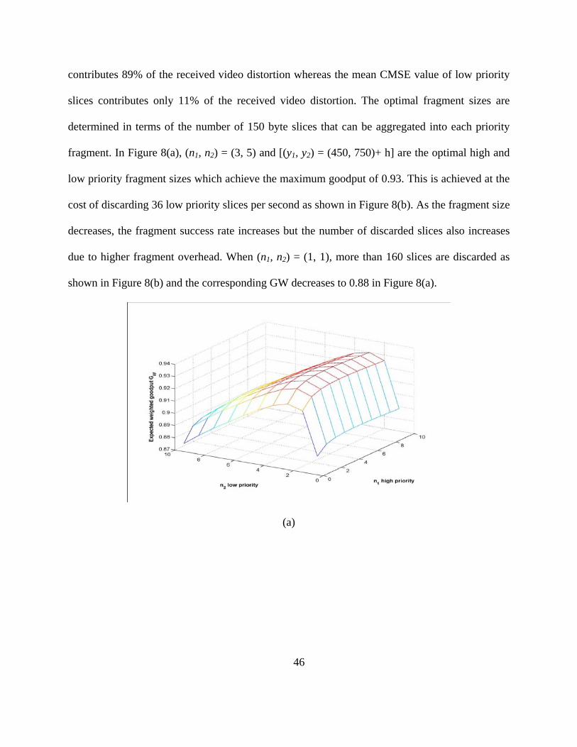
contributes 89% of the received video distortion whereas the mean CMSE value of low priority
slices contributes only 11% of the received video distortion. The optimal fragment sizes are
determined in terms of the number of 150 byte slices that can be aggregated into each priority
fragment. In Figure 8(a), (n1, n2) = (3, 5) and [(y1, y2) = (450, 750)+ h] are the optimal high and
low priority fragment sizes which achieve the maximum goodput of 0.93. This is achieved at the
cost of discarding 36 low priority slices per second as shown in Figure 8(b). As the fragment size
decreases, the fragment success rate increases but the number of discarded slices also increases
due to higher fragment overhead. When (n1, n2) = (1, 1), more than 160 slices are discarded as
shown in Figure 8(b) and the corresponding GW decreases to 0.88 in Figure 8(a).
(a)
46

(b)
Figure 8: (a) Expected Goodput, and (b) Slice discard comparisons between priority-
agnostic and priority-aware fragmentation.
Priority-agnostic vs. Priority-aware Fragmentation: We compare the performance of
priority-aware and priority agnostic fragmentation schemes in Figure 9. As shown in Figure 9(a),
priority-aware fragmentation achieves a goodput gain of 12% over priority-agnostic
fragmentation at R = 960 Kbps and pb = 10−4, even when it discards 8.25 Kbytes of additional
data during every transmission interval as shown in Figure 9(b). However, the performance of
priority-agnostic fragmentation starts converging with that of priority-aware fragmentation as the
channel BER decreases from 10−4 to 10−6. Figure 9(a) also shows that the priority-aware
fragmentation achieves a goodput gain of 18% over priority agnostic fragmentation at R=1080
Kbps and pb = 10−4. We discard 8.7 Kbytes of additional data to achieve this gain as shown in
Figure 9(b). Unlike R=960 Kbps, the priority-aware fragmentation achieves a goodput gain of
8% over priority agnostic fragmentation at lower BER (pb = 10−6) for R=1080 Kbps.
47

(a)
(b)
Fig. 9: (a) Expected Goodput, and (b) Slice discard comparisons between priority-agnostic
and priority-aware fragmentation
48

49
4.3 Simulation Results and Discussion
This section evaluates the performance of fragmentation schemes discussed in Section 4.2
and compares them to the baseline system. The baseline system does not include slice
prioritization and the packets are transmitted at the network limited MTU size of 1500 bytes.
Two standard CIF resolution (352 x 288) video sequences Foreman and Silent are used in our
experiments. They are encoded using H.264/AVC JM 14.2 reference software with GOP
structure IDR P B P B,….,P B at 30 frames/sec and encoding rates of 720 Kbps, 960 Kbps and
1080 Kbps. The GOP length is 20 and the rate control is enabled. Slice sizes of 150 byte, 300
byte, 600 byte and 900 byte are used and the slices are formed using dispersed mode FMO where
alternate macroblocks of a frame are arranged into two slice groups. The number of reference
frames for each P frame is set at 2 and the error concealment techniques are enabled. Motion
concealment is used as the temporal concealment technique for all the frames while spatial
interpolation concealment is used for errors in the reference frames. In the event of a complete
frame loss, concealment is done by copying the previous frame. The channel transmission rate is
1 Mbps and the PHY and MAC layer header h is set to 50 bytes.
4.3.1 Baseline System Performance
The three video encoding rates are chosen to resemble the corresponding cases (i) the
channel can support the video and allocate header bits to each fragment, (ii) the channel can
support the video but cannot allocate header bits to each fragment, and (iii) finally the channel
cannot support the encoded video rate. Figure 10 shows the error free PSNR (dB) for Foreman
and Silent video sequences at different encoding rates and slice sizes. The Silent sequence has
less motion compared to the Foreman sequence and hence it has better error free PSNR at the

50
corresponding encoding rates. In both the sequences the PSNR increases with increase in
encoding rate as well as slice size. As the slice size increases, more macroblocks are encoded in
a single slice which decreases the slice overhead. Since each slice is encoded independent of
other neighboring slices of the frame, a large slice size can more effectively exploit the spatial
correlation in neighboring macroblocks. In Figure 10, a 900 byte slice size provides a 0.4 - 0.5
dB gain in PSNR compared to a 150 byte slice size. Similarly, when the encoding rate is
increased from 720 Kbps to 960 Kbps, the corresponding PSNR also increases by 1 – 1.5 dB.
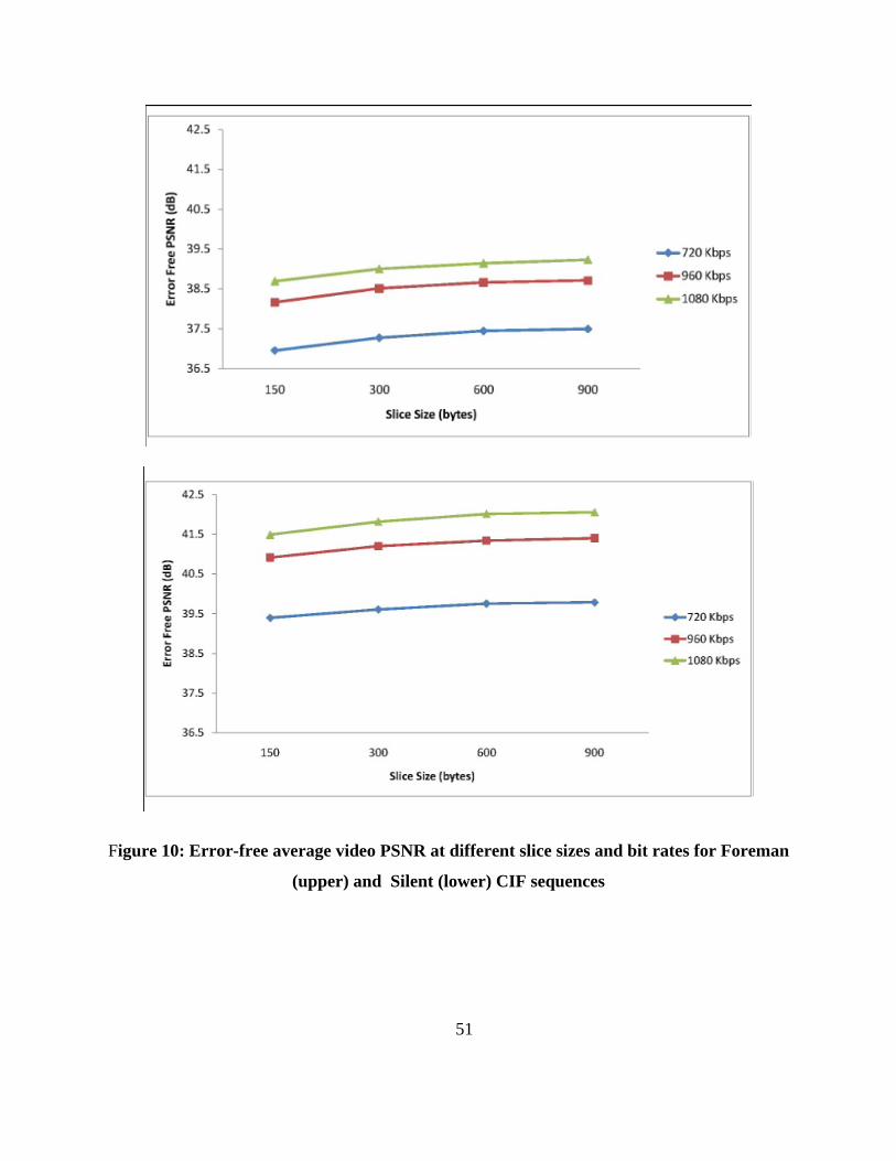
Figure 10: Error-free average video PSNR at different slice sizes and bit rates for Foreman
(upper) and Silent (lower) CIF sequences
51
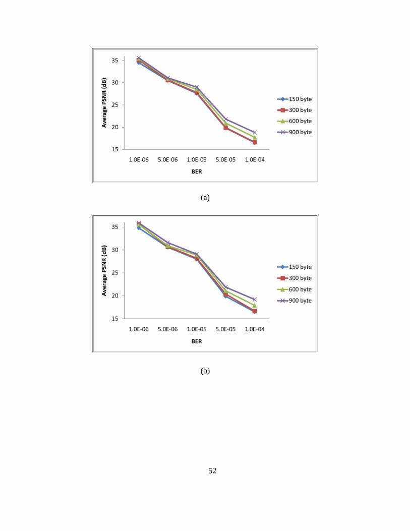
(a)
(b)
52

(c)
Figure 11: Average PSNR in baseline system for Foreman video sequence encoded at
(a) 720 Kbps, (b) 960 Kbps, and (c) 1080 Kbps.
Figure 11 shows the average video PSNR of Foreman sequence for the baseline system (i.e.,
1500 byte packets) with channel BER varying from 10-6 to 10-4. For a given video bit rate and
slice size, the video quality decreases as the BER increases because more packets with errors are
discarded at the receiver. The average video PSNR generally increases with slice size due to the
following reasons. First, the compression efficiency of smaller slices is lower than that of lager
slices. Second, 1500 byte MTU size would contain only two 600 byte slices or one 900 byte slice
which form a 1200 or 900 byte packet, respectively. On the other hand, 150 or 300 byte slices
form a 1500 byte packet. Since the packet error probability is a function of the packet size, the
900 or 1200 byte packets have fewer packet losses than 1500 byte packets. However the
corresponding video PSNR values at increasing channel BER are very low due to large packet
53
54
losses and this strengthens the need to perform fragmentation in order to increase the video
quality to an acceptable level.
Another observation is that, though encoding the video at higher target bit rate provides
better quality in error free channels as shown in Figure 10, the performance of video encoded at
1080 Kbps is poorer compared to videos encoded at 720 and 960 Kbps. This is due to the fact
that as the video bit rate exceeds the channel bit rate (1 Mbps) the excess packets have to be
discarded. This decreases the expected goodput G for the video encoded at 1080 Kbps as shown
in Figure 11(b) and results in poorer video quality. For example, G is about 50% for 1500 byte
slice size at channel BER of 5x10⁻⁵. Figure 11 also shows that the video PSNR remains the same
or increases only marginally in most cases when the video bit rate is increased from 720 to 960
Kbps for different channel BER’s. However this gain is small when compared to the 1-1.5dB
gain for the error-free channels in Figure 10. When the video bit rate increases more packets are
generated but at the same time more packets are also corrupted by channel errors. This decreases
the video quality gain that was achieved in the error-free case.
4.3.2 Priority-Agnostic Fragmentation Performance
Priority-agnostic packet fragmentation ignores the packet priorities and uses the optimal
fragment size derived by maximizing the expected goodput G as discussed in Section 4.2.3. The
average video PSNR achieved by the priority-agnostic fragmentation for the Foreman sequence
is shown in Figure 12. Like baseline system, the average PSNR in Figure 12 decreases when the
channel BER increases as well as when the video bit rate increases. However, the fragments
formed from smaller slice sizes provide better PSNR performance than the fragments formed
from larger slice sizes. This is because smaller slice size allows a finer aggregation of video data

into fragments as compared to large slice size. For example, each fragment contains eight and
two 150 byte slices at BER of 10-6 and 10-4, respectively, as compared to only one 900 byte slice.
For 720 Kbps video bit rate, the video quality is purely determined by the impact of channel
errors as sufficient bits are available to allocate header to each fragment. For 960Kbps and 1080
Kbps video bit rates, the fragment sizes may be higher and some slices are also discarded which
leads to more video quality deterioration at higher video bit rates and higher slice sizes.
(a)
(b)
55

(c)
Figure 12: Average PSNR achieved by priority-agnostic fragmentation for Foreman
video sequence encoded at (a) 720 Kbps, (b) 960 Kbps and (c) 1080 Kbps.
Figure 13 compares the expected goodput and video PSNR gains achieved by fragments
formed from 150 byte slice size over those formed from 900 byte slice size for the Foreman
video sequence. Both gains generally increase with BER for each video bit rate. At 720 Kbps
video bit rate and BER of 10-4, a large goodput gain of more than 45% and PSNR gain of 7.6 dB
is achieved. Similarly 31% gain in goodput is achieved at 960Kbps and 1080 Kbps video bit
rates with the corresponding PSNR gains of 4.6dB and 4.2dB, respectively.
56
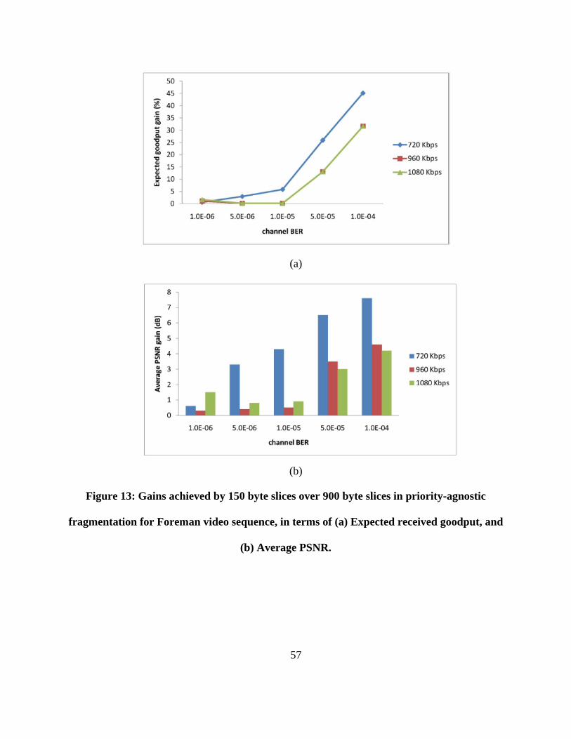
(a)
(b)
Figure 13: Gains achieved by 150 byte slices over 900 byte slices in priority-agnostic
fragmentation for Foreman video sequence, in terms of (a) Expected received goodput, and
(b) Average PSNR.
57
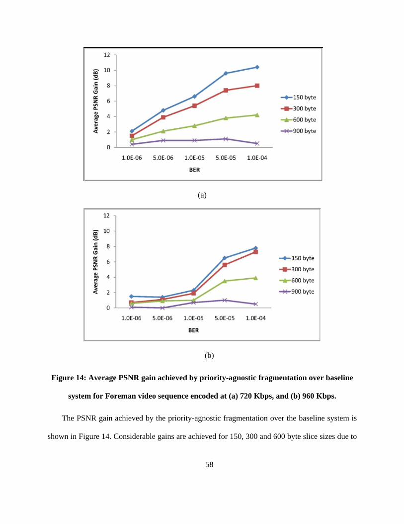
(a)
(b)
Figure 14: Average PSNR gain achieved by priority-agnostic fragmentation over baseline
system for Foreman video sequence encoded at (a) 720 Kbps, and (b) 960 Kbps.
The PSNR gain achieved by the priority-agnostic fragmentation over the baseline system is
shown in Figure 14. Considerable gains are achieved for 150, 300 and 600 byte slice sizes due to
58
59
enhanced fragment success rate in priority-agnostic fragmentation as compared to the baseline
system. The gain for these slice sizes generally increases with BER for 720 and 960 Kbps video
bit rate. Also the smaller slice sizes achieve larger PSNR gains as they can achieve finer
aggregation of video data in fragments as compared to the larger slice sizes as discussed in
previous paragraph. For example, a PSNR gain of 10.4dB is achieved for a 720 Kbps video
encoded using 150 byte slices at a channel BER of 10-4. For 900 byte slices, the gain is only
about 0.5dB. At a low channel BER of 10-6, the amount of gain achieved by different slice sizes
is almost the same since very few fragments are affected by error.
4.3.3 Priority-Aware Fragmentation Performance
In order to control the number of slices being dropped we adapt the fragmentation to the slice
priorities as explained in Section 4.2.3. Here, larger (smaller) fragment size is used for the low
(high) priority slices, along with fragmentation of slices. The prioritization of H.264 encoded
slices was explained in Section 4.2.2.
In order to increase the PSNR values as well as the corresponding gain achieved by the
priority-aware fragmentation, we propose a ‘distributed slice discard’ scheme in Figure 15 for
dispersed mode FMO for the two slices groups. This scheme gives highest importance to the
slice priority level, followed by the slice frame type and the selected slice group, in that order.
Priority level hierarchy ensures that the slices with the least distortion contribution are discarded
first. Frame type hierarchy causes the system to first discard the B-frame slices, followed by the
P-frame slices and finally the IDR-frame slices, if required. This strategy helps in controlling the
error propagation within a GOP as compared to the drop-tail mechanism. Since dispersed mode
FMO is used, if some slices from a slice group are discarded, the corresponding lost macroblocks

can be concealed from spatially adjacent macroblocks belonging to the other slice group. Since
the error concealment may not be effective when spatially adjacent macroblocks are discarded,
we discard slices from only one slice group in P and IDR frames. Since B frame slices do not
cause error propagation and can be effectively concealed, our scheme allows the discard of slices
from both B-frame slice groups.
Figure 15: Proposed slice discard scheme. Here Ds represents the number of bytes to
be discarded.
Priority-aware fragmentation maximizes the weighted expected goodput GW by increasing
the transmission reliability of high priority packets as discussed in Section 4.2.3. Figure 16 (a),
(b) and (c) show the expected received video PSNR for priority-aware fragmentation with the
proposed hierarchical slice discard scheme for Foreman video sequence. The variation of
average video PSNR with BER and slice size is similar to our observations for the priority-
60

agnostic fragmentation shown in Figure 12. In particular, we notice in Figure 16(a) and (b) that
the use of slice fragmentation in priority-aware fragmentation scheme has improved the PSNR
performance of large slice sizes and narrowed the gap between large and smaller slices sizes as
compared to the priority-agnostic fragmentation. However as discussed in Section 4.2.3, the loss
of first fragment containing the slice header causes the subsequent fragments of a packet to be
discarded at the receiver even though they were successfully received. This still keeps the
performance of large slices slightly inferior as compared to 150 byte slices when the channel
error rate is high and the resulting fragment success rate is low. Slice fragmentation of a large
slice also causes more slices to be discarded from the buffer when the video is encoded at high
bit rates and results in adjacent slices of the frame to be dropped. This causes the large slices to
underperform as compared to the 150 byte case even at low channel error rates at 1080 Kbps as
shown in Figure 16 (c).
(a)
61

(b)
(c)
Figure 16: Average video PSNR for priority-aware fragmentation of Foreman video
encoded at (a) 720 Kbps, (b) 960 Kbps, and (c) 1080 Kbps.
Table 4 and 5 show the video PSNR gains achieved by priority-aware over priority-agnostic
fragmentation ‘without using slice fragmentation’ for 960 Kbps Foreman and Silent video
62

63
sequences. The corresponding gain for 1080 Kbps video is shown in brackets. The priority-aware
fragmentation scheme adapts the fragment sizes to the individual packet priority levels as
explained in Section 4.2.3 which results in better received video quality. The PSNR gain
achieved at 1080 Kbps is almost same or greater than the gain at 960 Kbps. Please note that both
schemes have same PSNR performance at a video bit rate of 720 Kbps because the margin of
300Kbps for 1020 Kbps channel bit rate is sufficient to transmit each slice individually. At a
given channel BER it is also observed that higher gain is achieved at smaller slice sizes as
compared to large slice sizes. Please note that increasing the slice size decreases the flexibility in
choosing the fragment sizes as each fragment contains one or more slices in their entirety. For
example, fragment size can be either 600 bytes or 1200 bytes for a 600 byte slice size. Moreover
a 900 byte slice allows us only 1 slice/fragment at 1500 bytes MTU. This restricts the gain that
can be achieved by priority-aware over priority-agnostic fragmentation.
Table 4: PSNR Gains of Priority-aware over Priority-agnostic Fragmentation Scheme (Without Slice Fragmentation) for Foreman Video at 960 Kbps (1080 Kbps)
BER 10-6 5x10⁻⁶ 10-5 5x10⁻⁵ 10-4 150 byte 0.1 (1.6) 0.8 (1.4) 1.1 (1.6) 0.9 (0.7) 1.2 (1.4) 300 byte 0 (1.4) 0.9 (1) 0.9 (0.7) 0.5 (0.5) 0.1 (0.4) 600 byte 0 (1.2) 0.5 (0.6) 0.8 (0.7) 0.1 (0.5) 0.1 (0.3) 900 byte 0.1 (0.6) 0.6 (0.5) 0.2 (0.5) 0.1 (0.4) 0.1 (0.5)
Table 5: PSNR Gains of Priority-aware over Priority-agnostic Fragmentation Scheme (Without Slice Fragmentation) for Silent Video at 960 Kbps (1080 Kbps)
BER 10-6 5x10⁻⁶ 10-5 5x10⁻⁵ 10-4 150 byte 0 (1.9) 0.2 (2.4) 0.8 (2.1) 1.5 (0.6) 1.9 (1.9) 300 byte 0 (2.4) 0.6 (2.6) 0.7 (2) 1 (0.7) 0.7 (0.7) 600 byte 0.3 (1.9) 0.4 (2.2) 1 (2) 0.2 (0.5) 0.2 (0.3) 900 byte 0 (2.2) 0 (1.3) 0.3 (1.8) 0.2 (0.4) 0.2 (0.4)

64
Allowing the fragmentation of slices by suitably modifying the decoder to handle partial
slice data further increases the PSNR gain that can be achieved by priority-aware fragmentation
scheme as discussed below. Table 6 shows the PSNR gains achieved by priority-aware (with
slice fragmentation) over priority-agnostic fragmentation scheme for Foreman and Silent
sequences at 720, 960 and 1080 Kbps. The priority-aware fragmentation achieves better PSNR
as compared to the priority-agnostic fragmentation for all the slice sizes and BERs. For the
Foreman video sequence a maximum PSNR gain of 5.8dB is achieved at 720 Kbps and 900 byte
slice size at channel BER of 10-4 as shown in Table 6 (a). Similarly, 4.4 dB PSNR gain is
achieved for a video encoded at 960 Kbps for the same slice size and channel BER in Table 6
(b). The maximum gains for the Silent video sequence are 7.4dB is at 720 Kbps (Table 6 (a)) and
6.5 dB at 960 Kbps (Table 6 (b)) for 900 byte slice size and channel BER of 10-4. Similar gains
are also observed when the video encoding rate (1080 Kbps) exceeds the channel bit rate of 1
Mbps.
Table 6 (a): PSNR Gain of Priority-aware over Priority-agnostic Fragmentation
Scheme (with Slice Fragmentation) for Foreman (Silent) Video at 720 Kbps
BER 10-6 5x10⁻⁶ 10-5 5x10⁻⁵ 10-4
150 byte 0.4 (0.3) 0.2 (0.1) 0.1 (0) 0.1 (0) 0 (0.1)
300 byte 0.4 (0.2) 1 (0.8) 1.1 (0.9) 1.6 (1.7) 2 (1.7)
600 byte 0.6 (0.5) 2.5 (2) 2.7 (2.4) 4.1 (5.2) 4.1 (5.1)
900 byte 0.9 (0.8) 3 (3.3) 4.1 (3.9) 5 (6.7) 5.8 (7.4)

65
Table 6 (b): PSNR Gain of Priority-aware over Priority-agnostic Fragmentation
Scheme (with Slice Fragmentation) for Foreman (Silent) Video at 960 Kbps
BER 10-6 5x10⁻⁶ 10-5 5x10⁻⁵ 10-4
150 byte 0.2 (0.5) 1.1 (1.1) 1.2 (1.5) 1 (1.5) 1.3 (2)
300 byte 0.2 (0.1) 1.3 (1.4) 1.3 (1.1) 0.5 (1) 0.8 (1.8)
600 byte 0.2 (0.4) 1.1 (0.7) 0.9 (1) 1.3 (2.2) 2.7 (4)
900 byte 0.4 (0.1) 0.7 (0.6) 0.6 (0.9) 2.7 (4.3) 4.4 (6.5)
Table 6(c): PSNR Gain of Priority-aware over Priority-agnostic Fragmentation
Scheme (with Slice Fragmentation) for Foreman (Silent) Video at 1080 Kbps
BER 10-6 5x10⁻⁶ 10-5 5x10⁻⁵ 10-4
150 byte 1.6 (1.9) 1.4 (2.5) 1.6 (2.2) 0.7 (0.6) 1.4 (2)
300 byte 1.4 (2.5) 1.2 (2.6) 0.9 (2.6) 0.5 (0.8) 1.1 (1.5)
600 byte 1.5 (2.1) 0.8 (2.2) 0.8 (2.1) 1.7 (2.1) 2.7 (3.7)
900 byte 1.5 (2.3) 0.7 (2) 0.5 (2.3) 2.6 (3.6) 4.3 (5.8)
Figure 17 shows the 11th frame of Foreman sequence, encoded at 720 Kbps using an average
slice size of 600 bytes, subjected to a BER of 5x10⁻⁵. Figure 18 shows the 50th frame of Silent
sequence under the same specifications as the Foreman sequence.

(a) (b)
(c)
Figure 17: 11th frame of Foreman video sequence encoded at 720 Kbps and BER of
5x10⁻⁵ in (a) Baseline system: PSNR=20.3dB, (b) Priority-agnostic fragmentation:
PSNR=25.2dB, and (c) Priority-aware fragmentation: PSNR=29.9dB.
66

(a) (b)
(c)
Fig. 18: 50th frame of Silent video sequence encoded at 720 Kbps and BER of 5x10⁻⁵ in (a)
Baseline system: PSNR=22dB, (b) Priority-agnostic fragmentation: PSNR=28.5dB and (c)
Priority-aware fragmentation: PSNR=33.3dB
4.4 Conclusion
An efficient priority-aware adaptive packet fragmentation scheme was proposed to improve
the quality of pre-encoded H.264 bitstreams transmitted over unreliable error-prone wireless
67

68
links. The performance in terms of expected received video quality was compared to (a) the
traditional baseline model where each packet is transmitted onto the channel at the network
limited MTU size, and (b) priority-agnostic fragmentation scheme using a single optimal
fragment size. The optimal fragment sizes for the respective priority levels are derived using
branch-and-bound technique combined with multi-dimensional arithmetic interval methods.
Further slice fragmentation was used to boost the PSNR quality performance of videos,
especially encoded at large slice sizes. It is shown that maximizing the expected goodput or
expected weighted goodput provides large gains in received video quality.
The cross-layer priority information exchange between the video layer and MAC layer
allowed us to design an intelligent slice discard strategy which enabled us to reduce the impact of
lost slices on the received video quality. The proposed schemes can be easily embedded into
modern communication systems to assist in H.264 video streaming applications. The fact that
these gains are achieved without error correction techniques makes it all the more interesting to
evaluate the above strategies using unequal error protection for different priority levels.
69
5.0 ADAPTIVE MULTI-METRIC AD HOC ON-DEMAND MULTIPATH
DISTANCE VECTOR ROUTING
5.1 Introduction
Next generation mobile wireless ad hoc networks (MANETs) should be capable of
handling high node mobility to support a wide range of applications such as airborne and
vehicular networks [46, 47]. These networks are characterized by limited bandwidth and
unreliable channel conditions due to node mobility and multiple hops. Each node can directly
communicate to every other node if it is within its transmission range; otherwise it should
communicate with another node via multi-hop routing. The communication links between
source and destination nodes often break in a high mobility environment and the biggest
challenge is maintaining these links while keeping the delay and overhead minimum [48].
These characteristics pose a serious challenge in designing efficient routing schemes.
Ad hoc routing protocols can be categorized into proactive and reactive routing
protocols. In high mobility networks, proactive routing protocols generate too much overhead
because they find paths in advance for all source and destination pairs, even when no data is
being transmitted, and periodically exchange topology information to maintain them [48, 51,
52]. In contrast, reactive routing protocols have lower overhead as they find the route only
when there is data to be transmitted [49, 51, 54]. Depending on the functionality the ad-hoc
routing schemes can be grouped as (i) single path, (ii) multipath, and (iii) multipath with local
update. Single path routing schemes (such as such as ad hoc on-demand distance vector
(AODV)) establish a single route between the source and destination whereas the multipath
routing schemes (such as ad hoc on-demand multipath distance vector (AOMDV)) establish

70
more than one routes between the source and destination. The third category of protocols
(e.g., adaptive multi-metric AOMDV (AM-AOMDV)) deals with maintaining multiple paths
between source and destination along with local path update.
To provide robust communications, the reactive routing protocols adopt multipath
routing, path maintenance schemes, and link breakage prediction. Multipath routing protocols
(e.g., AOMDV) discover multiple disjoint and loop-free routes during the route discovery
phase. The link disjoint feature of this protocol ensures that no two parallel routes between a
source-destination pair will have a common link. If the currently used route fails, the source
chooses the next available route in order to continue packet transmission to the destination,
thus reducing routing overhead. However, the secondary routes, in high mobility ad hoc
networks, may become stale before primary route breaks. The source node would suffer data
loss if it switches to such an invalid route. To mitigate this problem, the path maintenance
schemes and link breakage prediction are used to detect and predict link failures,
respectively. The path maintenance schemes consist of link layer detection and hello message
[16]. The link layer detection utilizes link layer feedback to identify link failures during the
transmission of a data packet to another node. Periodic hello message is used by mobile
nodes to update the state of local connectivity. Link failure prediction adopts radio signal
strength and node mobility to estimate the status of links. When mobile node determines that
a link to its neighbor is likely to break, it sends a notification to its source node. Upon
receiving the notification, the source node can rediscover a new route (when using single path
routing) or switch to a secondary route (when using multipath routing).
The reactive routing protocols can therefore be characterized based on the number of
routes (single or multipath routing), path maintenance schemes (link layer detection or
periodic hello message) and route breakage prediction. Some routing protocols rely on path
71
maintenance schemes for link failure detection, while others rely on link breakage prediction
to preemptively bypass the weak links. Yet, some other protocols utilize local update to
strengthen primary routes, which is an extension of link breakage prediction. We have carried
out a comprehensive study of path maintenance schemes for single and multipath routing
schemes. Moreover, we compare the AODV and AOMDV schemes with our adaptive multi-
metric AOMDV (AM-AOMDV) scheme, using different path maintenance schemes, in a
wide range of node speeds, number of connections and packet rates.
The remainder of this section is organized as follows. In Section 5.2, we discuss the
related work. Section 5.3 describes the path maintenance schemes. We describe our new
multipath routing scheme, called as AM-AOMDV, in Section 5.4. In Section 5.5, we
compare the performance of single and multipath routing schemes. Finally, we discuss
conclusions in Section 5.6.
5.2 Related Work
Several papers have investigated how single path routing protocols perform in various
scenarios. A quantitative comparison of routing protocols, like Destination-Sequenced
Distance Vector (DSDV) [52], Temporally-Ordered Routing Algorithm (TORA) [53],
AODV and Dynamic Source Routing (DSR) [54], in terms of their implementations and their
working, is provided in [50]. The paper shows that DSDV and TORA perform worse in high
mobility environment. The paper also shows that AODV with link layer detection performs
as well as DSR at all mobility rates and accomplishes its goal of eliminating source routing
overhead. Lee and Gerla [51] showed that AODV provides a higher throughput and lower
latency than DSR in a congested network.

72
The AODV-Backup Routing (AODV-BR) scheme [68] uses the primary and alternate
paths which resembles a fish bone structure. Here a ‘primary route’ is created by the RREPs
as in AODV whereas an ’alternate route’ is a localized detour for the packet when a sudden
link break is detected in the primary route. When a node detects a route break, it forwards the
data packet instantly to the best alternate neighbor with an ‘alternate routing’ flag set in its
header, which will carry that packet to the destination. The AODV-Adaptive Backup Routing
(AODV-ABR) scheme [71] performs handshake process with its immediate neighbors to
repair the broken route instead of a one-hop data broadcast to its immediate neighbors. In
AODV-ABR, an aging technique is also used for alternate route maintenance. AODV-Break
Avoidance (AODV-BA) scheme [78] proposes flooding of RREQ’s which carry a unique
identifier to drop duplicate requests. A node may receive multiple RREP’s which form the
alternate paths, and when a link breaks a one hop broadcast is made to immediate neighbors
which switch from primary to the alternate route. A timer mechanism is used to distinguish
between stale and new routes. The AODV-Accessibility Prediction (AODV-AP) scheme [74]
maintains status of active nodes based on their accessibility. A neighborhood table is
maintained with the help of some timers. This scheme has a lower routing overhead than
AODV. The AODV-Preemptive Local Route Repair (AODV-PLRR) scheme [79] aims to
avoid route failures by preemptively repairing the local routes when a link break is about to
occur. “HELLO” messages are used for maintaining neighborhood connectivity in this
scheme. An enhancement to AODV is proposed in [83], which uses joint nodes’ packets
delivery records, current nodes’ traffic load and routes’ hop count information as route
selection criteria to select low delay and more stable routes. The Load Balancing AODV
(LB-AODV) scheme [75] is a modification of AODV to meet load balancing requirements.
73
In Robust AODV scheme [73] the route is built on demand but maintained by local proactive
route update.
The multipath extension to AODV and DSR were proposed in [49] and [59],
respectively. The multipath routing protocols establish multiple disjoint paths between source
and destination thereby improving network resilience to link failures and allow for network
load balancing. Route maintenance in AOMDV is merely an extension of AODV and uses
the RERR messages to detect a broken link. AOMDV also includes an optimization to
salvage packets forwarded over failed links by re-forwarding them over alternate paths.
Marina et al. [49] states that multipath routing protocols require link layer detection and hello
message to maintain multiple routes. Various single and multipath protocols, like AODV,
DSR, Split Multipath Routing (SMR) [61], AODV-Multipath [62] and AOMDV have been
compared in [60]. The results show that SMR, a modification of DSR, performs best in
network with low node density but degrades as the network density increases while AOMDV
performs well under high mobility scenarios as opposed to AODVM which is best suited for
static networks. However, the paper only conducted performance comparisons for low node
mobility [0,10m/sec]. Moreover, the paper established that multipath routing works better in
dense networks with high traffic load as compared to single path. [62] and [63] discuss
modifications of AODV for achieving multiple paths while keeping the overhead fixed.
Unlike using the multiple routes in AOMDV, the LHAOR (Link Heterogeneity Aware
On-demand Routing) scheme [90] strengthens the main route by using a local update scheme
for generating surrogate routes. This scheme uses a path information exchange mechanism
between neighboring nodes and introduces RSSI as a new routing metric. However the single
route concept could cause significant end-to-end latency in data transmission when a
significant number of links fail. [64 - 66] discuss the modifications to AOMDV to meet QoS

74
requirements. The performance of AODV and AOMDV schemes is compared in [66] under
different network conditions for CBR traffic. MM-AOMDV [69] suggests a multi metric and
multipath routing scheme which chooses its paths depending on the combined metrics that
effectively determine the load. This protocol is effective for load balancing applications. [70]
proposes to probabilistically select paths based on end-to-end transmission delay as the cost
metric. The authors point out that the transmission delay is more sensitive to varying data
traffic than any other metric. Scalable Multipath On-Demand Routing (SMORT) [71]
computes multiple fail-safe paths between source and destination which are fail safe to the
primary path if it bypasses at least one intermediate node on primary path.
The QoS enabled Node-Disjoint Multipath Routing Protocol (NDMR) [77] supports
multimedia applications by reducing end to end delay, optimizing bandwidth etc. RREP
packets should carry more information such as delay time (queue length) to meet service
level agreement (SLA) requirements. Adaptive QoS (ADQR) [80] employs a different route
discovery algorithm to find multiple disjoint paths with longer lived connections. Here each
path also specifies associated network resource information which provides an efficient
approach for network resource reservation combined with data dispersion and for route
maintenance. This provides lower bandwidth utilization due to longer lived connections
which requires lower route maintenance. Dynamic MANET On-demand Multipath
(DYMOM) [82] proposes a multipath routing scheme which uses multiple node disjoint
routes to the destination for load balancing applications. AODVM with Source Lists [81]
proposes to use a new route update procedure with combined metrics of delay, hop count and
disjointness, and each intermediate node deliberately selects multipath candidates while
contributing to suppression of unnecessary routing packets. Extension of RREQ/RREP
75
packets with a source route list is also incorporated, not only to alleviate limitation of the
hop-count based approaches but also to provide multiple routes.
Some more modifications made to AODV and AOMDV to suit frequent topology
changes and adapt to dynamic network conditions have been mentioned below. [85] is merely
an extension of AODV that finds multiple node disjoint paths but fails to perform when the
network becomes dynamic. [86] is a modification made to AOMDV using a concept referred
to as zone disjoint paths. By this we mean the nodes have no neighbor in the other path. It
uses active neighbor count and eliminates the route cache to be maintained in intermediate
nodes. Additionally the duplicate RREQ’s are not discarded and rather stored in an RREQ
table. The above protocols work best in low mobility and low network load conditions. [87]
refers to the optimizations introduced in AOMDV in order to make the protocol more
resilient to dynamic situations. A neighbor information table is augmented to the periodic
beacons to carry information about its present status. This table also contains signal strength
from neighboring node which helps in dynamically deciding the route. This optimization
ensures efficient load balancing when the network is congested. [88] works by addition of
overhead to each packet which is calculated as the linear function of the original packet. A
scheme is devised to offer protection against path failures using diversity coding so that the
network can quickly adapt to dynamic topology changes.
[63] compares the effect of MAC on different protocols and evaluates their
performance. This analysis helps in learning about the influence of link layer feedback and
periodic hello beacons on the performance of single and multipath routing protocols. While
link layer detection provides rapid link failure detection, it also introduces false link layer
failure detections when data transmission rate is high and short-term link quality variations
occur. [64] proposes veto mechanism to reduce spurious link layer failure detections and
76
implements packet salvaging to improve packet delivery ratio, reduce end to end latency and
overhead. [55] conducted performance comparisons between single path routing protocols
(e.g., AODV, DSR, Optimized Link State Routing (OLSR) etc.) with and without link layer
detection. The protocols with link layer detection have higher packet delivery ratio than the
protocols without link layer detection. This is because the link layer detection is able to
identify link failures quickly. [56]-[58] also demonstrate that AODV with link layer detection
performs better than conventional AODV.
To the best of our knowledge a thorough study of single and multipath routing protocols
with and without link layer detection in high mobility ad hoc networks has not been
considered. We have conducted a thorough study of single and multipath routing protocols
with and without link layer detection in high mobility ad hoc networks in varying network
conditions. Our aim in this paper is to analyze the performance of various single and
multipath routing protocols and compare this against our scheme AM-AOMDV. Most
authors have compared the performance of AODV against AOMDV by restricting node
speeds to 20 m/sec [e.g., 49, 50]. However, we have conducted tests to evaluate the behavior
of these schemes under higher node speed as well as congested networks.
5.3 Path Maintenance Schemes
The topology changes in mobile ad-hoc networks results in short lived links. This calls
for the need of path maintenance schemes which deal with link failure detection. When link
breaks, data packets will be queued in the mobile nodes because they cannot be sent via
alternate routes. If the packets are unable to be salvaged, they are dropped. In such a case,
mobile nodes need to detect it as soon as possible in order to reduce end to end latency and
packet dropping rate. According to [16], there are two path maintenance schemes: link layer
detection and hello message. They operate in link layer and network layer, respectively. In
77
the following paragraphs, we discuss the hello messages and link layer detection schemes,
followed by their advantages and disadvantages.
Hello Messages are periodic locally broadcast messages that are used to indicate link
availability. Hello messages may be used to detect and monitor links to neighbors. Each
active node periodically broadcasts a hello message that all its neighbors receive. Because
nodes periodically send Hello messages, if a node fails to receive several Hello messages
from a neighbor, a link break is detected. The amount of time it takes to detect a link break in
AODV using Hello messages depends on two parameters: allowed_hello_loss and
hello_interval [53]. However, the HELLO messages often interfere with the data transmission
on the same or other closely spaced routes.
Link layer feedback is defined as notification, sent from the link layer to the routing
layer, that a link to a neighbor has been broken [55-57, 64]. This feedback is assumed to be
provided by the underlying MAC protocol, in our case IEEE 802.11. In IEEE 802.11, a data
packet is first queued for transmission at the MAC layer. If the packet cannot be transmitted
after multiple MAC layer retries, an indication is given, to the higher layers that a failure has
occurred.
Link layer feedback quickly identifies the link failures during transmission of a data
packet to another node, while periodic hello messages have longer link detection latency.
When link layer detection is used, fewer data packets are lost and the route can be repaired
quickly [53, 55]. However, link layer feedback is not realizable in current hardware and
hence it can only be simulated [55, 56]. It also generates considerable false detections when
the packet sending rate is high and short-term link quality variations occur [56]. In addition,
link layer detection only allows node to detect the status of the link to its next hop along the
current route. Without hello message, node cannot know the status of its neighbors.

78
Additionally, promiscuous listening mode is enabled whenever Hello messages are utilized
which enables link failure detection [63].
5.4 Method: Description of AM-AOMDV Routing Scheme
We describe below the major features of our AM-AOMDV routing scheme.
5.4.1 Multiple Routing Metrics
AOMDV uses the minimum hop-count as the link metric in the route setup stage for
choosing the shortest path from the source to destination. This does not necessarily support
data transmission in high speed environments since minimum hop-count based metric does
not consider the RSSI (received signal strength indication) degradation on multihop links
(due to interference).
We use a novel multiple metric approach for converging to the most efficient route while
discovering multiple routes in the route setup stage. These metric values are introduced in the
routing table for each node and their corresponding paths. The enhanced routing table
contains three additional metrics: (a) node-to-end RSSI metric, (b) node-to-end latency
metric, and (c) node occupancy metric. The node to-end RSSI metric is defined as the RSSI
value of the path from any node to the destination. We use average value of RSSI. The RSSI
value of each forward link is fed back to the nodes through the ACK packets. The node-to-
end latency metric consists of two parameters (i) delay from the node to the source computed
from the timestamp of the RREQ packet, and (ii) the delay from the destination to the node
computed from the RREP packet. The node occupancy metric is defined as the total number
of data packets that any node processes per second and plays an important role under heavy
traffic conditions where hot spots are likely to be created in the network. The AM-AOMDV
79
scheme uses these metrics along with the hop-count metric to find the new paths and select
the best one intelligently.
5.4.2 Route Setup Stage
Every node maintains a routing table which is updated whenever it receives a RREQ
(Routing REQuest), RREP (Routing REPly) or a local update HELLO packet. When the
application layer sends a packet to the routing queue, the source looks for a route to that
destination in its routing table. If a valid route is available the node enters the data
forwarding state and forwards the packet to the first hop node of the appropriate route.
However, if no route is available and the node is the source of the data packet, it enters the
route discovery state, which is similar to the AOMDV scheme [50]. In this state, the node
broadcasts RREQs for finding the routes to destination. Each intermediate node re-broadcasts
the received RREQs and sets up a backward route towards the source. During this phase,
each intermediate node discards multiple RREQ packets from the same former relay node to
avoid looping and the same sequence number to guarantee link disjoint routes. Moreover the
next hop and last hop information are also used for checking node disjoint routes. Finally,
when one of the RREQ packets reaches the destination node it sends an RREP back to the
source node using the backward routes (appropriate to that RREQ packet) stored in each
intermediate node in the reverse direction. The destination floods RREP’s in the reverse
direction similar to the number of multiple RREQ’s received from the source. The RREQ-
RREP pairs form multiple routes from source to destination [50].
After receiving the first RREP from destination, the source starts forwarding data
packets. If a new reply arrives after the source has entered data forwarding state with a better
routing metrics, the source will switch to the new route. This is because our proposed scheme
is inherently adaptive and chooses the best available route, unlike AOMDV. In the event of a

80
link breakage the intermediate node enters into a route maintenance state after a repeated
number of unsuccessful attempts made by it to forward the data packet. It interprets the
situation as a route error and transmits an RERR (Route ERRor) packet in a unicast manner
on the backward route to the source. This process causes all the nodes to delete the next hop
to the destination in their routing tables along that route.
5.4.3 Data Transmission using Local Path Update
The number of routes from the source to destination is restricted to a heuristic upper
bound and the source begins data transmission on the route identified by the first received
RREP packet. This route is labeled as the primary route whereas the other routes are labeled
as secondary routes. All the nodes through which the RREP packet(s) travels from the
destination to the source are marked as Forward Route (FR) nodes. When the first FR node
on the primary route receives a data packet, it starts participating in the local path update
process by broadcasting a HELLO message to its 1-hop neighbors. The HELLO packet
contains path information from its routing table. A flag in the HELLO message identifies the
originator of the packet, which enables the neighboring FR nodes to discard this HELLO
broadcast. The 1-hop neighboring non-FR nodes, which hear this local update HELLO
message, either add a new route entry or update the existing routing information. These 1-hop
neighbors of the FR nodes are labeled as Surrogate Route (SR) nodes. These SR nodes help
in setting up alternate routes to the destination by receiving periodic local updates from their
1-hop FR neighbors. The SR nodes respond to the local update HELLO messages received
from an FR node, by broadcasting another local update HELLO but with the flag reset inside
it. This enables other FR nodes to accept this HELLO broadcast from the SR nodes and add
new paths in their routing table or update existing paths, if they are found to be better in
terms of the multiple metrics described in Section 5.4.1. This causes the primary route to
81
converge to a more efficient route and thus prolong the route life-time. After receiving the
first data packet, the SR nodes label themselves as FR nodes and begin the local path update
process again.
5.4.4 Enhanced Link Layer Failure Handling
When the MAC layer does not receive a CTS (clear to send) packet even after
retransmitting the RTS (request to send) packet for a short retry limit, the situation is
interpreted as a link failure. The MAC layer reports this to the routing layer through a
callback mechanism and a packet salvage process is initiated by finding alternate routes to the
destination in its routing table. If no route is available to the destination, the data is dropped
and an RERR packet is transmitted in a unicast manner on the backward route to the source.
Due to the lack of local route update, the AOMDV scheme cannot always salvage the packets
and drops them which results in large packet loss and routing overhead when node mobility is
large. On the other hand, our proposed routing approach periodically updates the route to the
destination using the local update algorithm. It not only strengthens the path locally and
ensures longer route life-time but also delivers more packets to the destination.
5.4.5 Keep Alive Mechanism: Secondary Route Maintenance
AOMDV does not maintain or locally repair the secondary routes. As a result, the
secondary route may also fail and may not be available for data transmission after the
primary route has failed, especially when node mobility is high. Consequently, the route
discovery frequency increases in AOMDV in the presence of high node mobility. Our scheme
uses the keep alive packets to monitor the secondary routes and heal any link breakages. If
any FR node does not find a valid next hop it initiates a local one hop repair query, asking its
neighbors for a route via the same last hop. Non FR neighbors having paths to the destination
82
via the required last hop reply to this query. Thus the FR node immediately adds one of these
neighbors as a new next hop in its routing table. When the keep alive packet reaches the
destination, it retransmits the same on the reverse route to the source via that secondary path
and updates the multiple metrics in both the forward and reverse directions. This mechanism
thus periodically updates the secondary routes and reduces the route discovery frequency.
5.5 Effectiveness of AODV, AOMDV and AM-AOMDV
Reactive protocols like AODV tend to reduce the control traffic messages overhead at
the cost of increased latency in finding new routes. AODV has a lower bandwidth
requirement as control packets are smaller control and data packets. The protocol is scalable
since it has to record only two addresses, i.e., destination and next hop. Disadvantage is that
this protocol has to reinitialize route discovery when path fails. This causes long end to end
latency and high packet drops. The advantage of using AOMDV is that it allows source nodes
to find multiple paths during route discovery process. Therefore, it decreases RREQ, thereby
increasing packet delivery ratio. Furthermore, AOMDV allows intermediate nodes to reply to
RREQs, while still selecting disjoint paths. The primary disadvantage of AOMDV is due to
the fact that there are more messages, overhead during route discovery due to increased
flooding and intermediate nodes reply to multiple RREQ’s increasing the control overhead
and complexity. Multipath routing can result in packet reordering and hence the allocation of
packets on multiple routes should be taken into account.
AM-AOMDV performs considerably better than legacy AOMDV especially in high
mobility and high number of flows and matches the performance at low mobility and low
number of connections. It shows a higher throughput, a lower end to end delay and reduces
the total routing overhead to half of that of legacy AOMDV. The need for route discovery in
AM-AOMDV is always lower than in legacy AOMDV essentially because of its local update

83
mechanism. It also trades off the Route Discovery latency for achieving a much lower routing
overhead, thus causing a slight increase in the route discovery latency at low node speed and
less connections. The average path length in AM-AOMDV matches with legacy AOMDV
implying that AM-AOMDV never trades hops for other metrics. Thus AM-AOMDV’s
characteristics make it suitable for highly mobile ad hoc networks with a high number of
flows.
5.6 Simulation Results and Discussions
The simulations are conducted in network simulator (ns2). In this paper, we evaluate
AODV and AOMDV using different path maintenance schemes (i.e., link layer detection and
hello). We abbreviate those protocols as AODV-LL, AODV-HELLO, AOMDV-LL,
AOMDV-HELLO, Legacy-AOMDV and AM-AOMDV. Here the legacy-AOMDV enables
both link layer detection and periodic hello message. In the following paragraph, we outline
the simulation environment setup, which is followed by the performance comparisons of the
routing protocols by varying node speed, varying number of connections, and varying packet
rate.
5.6.1 Simulation Setup
In NS2, the distributed coordination function (DCF) of IEEE 802.11 for wireless LANs
is used at the MAC layer. The radio model uses characteristics similar to Lucent’s WaveLAN
radio interface. We use an error-free wireless channel model. Table 7 summarizes the
parameters used in our simulation setup. It is important to note that the nodes can serve as
source as well as destination in the network. We run each simulation for 1000 seconds and
ignore the initial 250 seconds as done in AOMDV protocol, which is considered as a warm-
up period. Each simulation is run 5 times and the results are an average of the 5 observations.

84
Therefore each point represents a simulation of five unique traffic movement patterns. We
repeat the simulations for different traffic (connections and packet rate) variations and
mobility models (mean node speed).
Table 7: Simulation Parameters
Parameters Values Network size 1000m X1000m
Number of nodes 100 Propagation model Two ray ground Transmission range 250m
Simulation time 1000 seconds with 0 pause time Traffic type Constant bit rate (512byte packets)
MAC protocol IEEE 802.11 b Link bandwidth 2Mbps
Interface queue length Drop/Tail PriQueue of 50 Mobility model Random way point
Remaining simulation parameters are described below:
• Description of data packet: 50 CBR/UDP connections are used in low and high node
density networks, respectively. Packet rate is set to 1 packet per second with packet
size of 512 bytes. These correspond to the offered loads of around 200 Kbps. The
interface queue size is limited to 50 packets.
• Scenarios: We have conducted simulations extensively for three cases wherein we
have varied the node speed between 1-30m/sec keeping other parameters fixed with a
packet rate of 1pkts/sec and 50 connections. In another set of experiments we have
varied the packet rate between 0.25-1pkts/sec fixing other parameters with a node
speed at 20m/sec and connections at 50. We have conducted tests by varying number
of connections between 10 -50 connections and fix node speed to 20m/sec and packet
rate to 1pkts/sec.

85
• Performance metrics: (1) Throughput per flow: ratio of number of packets transmitted
at source nodes to number of packets received at destination nodes per flow; (2)
Average end to end latency: average transmission delay of data packets, which
includes queuing delay, propagation delay, retransmission delay, etc.; (3) Normalized
routing overhead: number of control packets transmitted per data packet received; (4)
RREQ frequency: total number of RREQ’s sent by the source per second.
5.6.2 Performance Comparison by Varying the Node Speed
Fig. 19 shows the performance comparison between AODV-LL, AODV-HELLO,
AOMDV-LL, AOMDV-HELLO, Legacy-AOMDV and AM-AOMDV schemes when node
speeds vary from 1 to 30 m/s. As shown in Fig. 19(a), up to node speed of 10 m/sec the
corresponding single path and multipath routing schemes give similar throughput per flow
because the node speed is low and the topology varies slowly. For example, the AODV-LL
and AOMDV-LL have similar throughput performance. Similarly, AODV-HELLO and
AOMDV-HELLO have similar performance. Similarly, Legacy-AOMDV and AM-AOMDV
schemes have similar performance and outperform the remaining four schemes.
For node speeds above 10m/s, the throughput drops with increasing node speed because
the routes are more likely to break and the additional number of control messages are sent for
route maintenance and route discovery. Specifically, AM-AOMDV performs better than the
remaining schemes because it has better local route update mechanism. It is observed that
AODV-LL, AOMDV-LL and Legacy-AOMDV have higher throughput per flow than the
HELLO based schemes because the link failure detection is faster than the hello messages
and is without overhead. Legacy-AOMDV has higher throughput than the AODV-LL up to a
node speed of 15 m/s. However, its throughput drops below that of AODV-LL for higher

node speeds. AODV-LL and Legacy-AOMDV both use link layer detection for link failure,
but the AODV-LL initiates the new route discovery when the primary path fails while the
Legacy-AOMDV uses hello messages to maintain secondary routes. However the rate at
which hello messages detect link failure may lead to routes becoming stale while still adding
the HELLO message overhead, which leads to slightly lower throughput. As the control
messages increase, the probability of dropping data packets increases. AOMDV-LL has
slightly lower throughput than the Legacy-AOMDV at the node speeds of above 10m/s
because it does not update the secondary routes which also break up due to high mobility by
the time the primary route is broken.
(a)
86

(b)
(c)
87

(d)
Figure 19: Performance of different routing schemes for varying node speeds: (a)
throughput per flow, (b) Average end-to-end latency, (c) Normalized routing load, and
(d) Number of RREQ’s per second.
Fig. 19(b) shows that the AODV-LL and AM-AOMDV have average end-to-end latency
below 300ms which is lower than that of other four schemes. AODV-LL has the lowest end
to end latency because it has a lower number of control packets as compared to other schemes
which reduces the bandwidth consumption. Additionally the link failure detection latency is
very small. This was also observed in [51]. AM-AOMDV has a low end-to-end latency due
to local repair of routes which keeps the overhead under control and results in lesser route
breaks avoiding additional retransmissions of packets and higher throughput. AM-AOMDV
has a slightly higher end-to-end latency than AODV-LL at node speeds above 10 m/s which
could be due to relatively higher throughput achieved by AM-AOMDV (see Fig. 19(a) and
88

89
discussion in paragraph above). AODV-HELLO and Legacy-AOMDV have highest end-to-
end latency as they generate a larger number of control packets for path maintenance which
increases with the node speed. Overall, the latency increases with the node speeds for all the
schemes. The probability of link failures and new route discovery frequency increases with
the node speed, which necessitates the need to send out more control packets which accounts
for additional delay [55]. AOMDV-LL is not aware of secondary route failures, which are
more likely to break at higher node speeds, as it does not use HELLO messages on the
secondary routes. As result, it attempts to send data packets through secondary route when
the primary route breaks. These packets thus get delayed before being sent on a new route
which leads to higher end-to-end latency. Higher end to end latency in AODV-HELLO could
be due to the fact that HELLO messages have slower link failure detection which would
delay packets in the node queue and also add the overhead.
Fig. 19(c) shows the number of RREQs generated per second (known as RREQ
frequency hereafter in this paper) for varying node speeds. We observe that AODV-LL has
the highest value because it has up to 30 times higher rate of false link failure detections as
compared to HELLO messages. This initiates more frequent discovery leading to a much
higher number of RREQs at the source. Legacy-AOMDV and AOMDV-LL, which use link
layer failure detection mechanism, also have higher RREQ frequency than the remaining
three schemes which use HELLO messages. However, their RREQ frequency is much lower
than that of AODV-LL due to the use of multiple paths. AM-AOMDV has the least value
since it has the mechanism of local update through which the primary paths are strengthened
and they maintain secondary routes thereby reducing the number of RREQ’s generated [24].
Fig. 19(d) shows the normalized routing overhead which generally increases with node
speed. AODV-HELLO and AOMDV-HELLO have the maximum overhead because they use

90
periodic broadcasting of HELLO messages. Legacy-AOMDV has a slightly lower overhead
as compared to AOMDV-HELLO since it first uses the link layer detection, followed by the
HELLO messages, for path maintenance. Although AODV-LL and AOMDV-LL do not use
HELLO messages, they have much more frequent route discovery (as explained above in the
previous paragraph). As a result they have only a slightly lower overhead than the HELLO
based schemes. Furthermore, the AODV-LL has slightly higher overhead than the AOMDV-
LL because the later uses multiple paths. AM-AOMDV has the lowest overhead because it
uses controlled HELLO’s broadcast and local update feature which strengthens the primary
path and maintains secondary routes hence reducing the RERR messages and consequently
reducing the frequency of RREQ’s generated at the source.
5.6.3 Performance Comparison by Varying the Number of Connections
Fig. 20 shows the performance comparison between AODV-LL, AODV-HELLO,
AOMDV-LL, AOMDV-HELLO, Legacy-AOMDV and AM-AOMDV in a network by
varying the number of connections.
In Fig. 20(a), as number of connections increases the throughput per flow decreases due
to more packet collisions. AM-AOMDV has the highest throughput per flow since it uses the
mechanism of local update which helps in path strengthening. Additionally it maintains
secondary routes because of the packet delivery ratio are sustained. The throughput for
AODV-LL is better than AOMDV-LL when the number of connections is higher than 25,
because the latter use multiple paths which generates more control packets in an already
congested network leading more packet drops in the node queues. Legacy-AOMDV and
AOMDV-LL have similar throughput as they both are multi-path schemes. The throughput
for HELLO based AODV-HELLO and AOMDV-HELLO schemes are the lowest because
they generate more control packets which add to the overhead. For up to 30 connections, both

91
schemes have similar performance. However, as number of connections increases beyond 30,
the AOMDV-HELLO shows better throughput than AODV-HELLO because AOMDV-
HELLO has backup routes while AODV-HELLO has to reinitiate route discovery whenever
primary routes fail.
As shown in Fig. 20(b), the AODV-HELLO scheme has the highest average end-to-end
latency because of higher control packet overhead (due to HELLO messages) which
contributes to the network congestion and increased packet delay in the node buffers. As
discussed in the previous paragraph, this also leads to the lowest throughput per flow.
Similarly, the use of HELLO messages also results in higher average end-to-end latency for
AOMDV-HELLO scheme. However, it has lower latency than AODV-HELLO due to the use
of multiple paths. On the other hand, AODV-LL and AM-AOMDV have average end-to-end
latency below 300ms which is lower than that of other four schemes. These two schemes also
have the higher per flow throughput as shown in Fig. 20(a). AODV-LL has the lowest end to
end latency because it has a lower number of control packets as compared to other schemes
which reduces the bandwidth consumption. Additionally the link failure detection latency is
very small. This was also observed in [51]. AM-AOMDV has a low end-to-end latency due
to local repair of routes which keeps the overhead under control and results in lesser route
breaks avoiding additional retransmissions of packets and higher throughput. Furthermore,
AOMDV-LL and Legacy-AOMDV schemes have almost same latency which is higher than
that of AODV-LL and AM-AOMDV schemes for more than 35 connections due to higher
control overhead. Please note that these two schemes (i.e., AOMDV-LL and Legacy-
AOMDV) also have similar throughput as discussed in Figure 20(a).
The RREQ frequency of different schemes shown in Fig. 20(c) follows the similar trends
as in Fig 19(c). Here, AODV-LL has the highest RREQ frequency because it has up to 30

92
times higher rate of false link failure detections as compared to HELLO messages as
discussed in [64]. This initiates more frequent discovery leading to a much higher number of
RREQs at the source. Legacy AOMDV and AOMDV-LL have similar RREQ frequencies
since they both are multipath routing schemes and use link failure detection. This frequency
is lower than AODV-LL since in multipath protocols route discovery is not initiated until all
routes to destination fail. AODV-HELLO and AOMDV-HELLO schemes suffer because
both data and control packets are queued adding to route discovery latency. AM-AOMDV
has the least RREQ frequency since it uses a local update mechanism wherein the primary
path is strengthened and secondary routes are maintained which reduce the number of
RREQ’s generated by the source.
The normalized routing overhead shown in Fig. 20(d) is high for the HELLO-based
routing schemes (i.e., AODV-HELLO, AOMDV-HELLO and Legacy-AOMDV) for low
number (up to 15) of connections and decreases thereafter for up to 30 connections (or 40 for
some schemes). This is explained below: In Section 5.6.1, the normalized routing overhead
was defined as the ratio of total number of control packets to the total number of received
data packets. In these schemes, the HELLO messages are generated by each node irrespective
of the number of connections, thus generating high control overhead. At the same time, the
total number of received data packets is a function of the number of connections which
governs the number of packets generated at the source. As a result, the number of data
received packets would be low for lower number of connections whereas the control
overhead remains relatively high. Since the two link layer based schemes do not have
HELLO messages and the AM-AOMDV scheme uses much lower number of HELLO
messages, we do not observe this behavior. Furthermore, the normalized routing overhead for
AODV-HELLO increases beyond 30 connections because the per flow throughput which

93
represents the number of received packets considerably decreases as shown in Fig. 20(a).
Please note that the per flow throughput does not decrease considerably for higher number of
connections for other schemes, which explains no or very small corresponding increase in
normalized routing overhead.
As shown in Fig 20(d), the AODV-HELLO scheme has the highest normalized routing
overhead due to higher number of control packets. Please note that this scheme also has the
highest end to end latency and the lowest throughput per flow which also implies a high
overhead. Although the AOMDV-HELLO and AODV-HELLO have the same throughput up
to 30 connections, the AOMDV-HELLO has lower normalized overhead due to its multipath
mechanism, which is also demonstrated by lower RREQ frequency in Fig. 20(c). AOMDV-
HELLO has a higher overhead initially but then becomes comparable with Legacy-AOMDV
since the values of control messages generated when the number of connections increases
remains almost same. Their RREQ frequencies are also comparable as shown in Fig. 20(c).
This explains the reason for the converging curves.
In Fig. 20(d), AODV-LL has more overhead than AOMDV-LL because the latter
maintains multiple paths which reduce the number of new path discoveries when the current
paths fail as also seen in Fig. 20(c). AM-AOMDV achieves a reduction in overhead which is
almost half of that of Legacy AOMDV because of the use of controlled HELLO message
broadcast. Furthermore, AM-AOMDV has local update feature which strengthens the
primary path and maintains secondary routes hence reducing the associated control messages
including the number of RREQs generated at the source.

(a)
(b)
94

(c)
(d)
Figure 20: Performance of different routing schemes for varying number of
connections: (a) throughput per flow, (b) Average end-to-end latency, (c) Normalized
routing load, and (d) Number of RREQ’s per second.
95

96
5.6.4 Performance Comparison by Varying the Packet Rate
Fig 21(a) shows the per flow throughput for the routing schemes under consideration.
AODV-HELLO and AOMDV-HELLO perform poorly because of the large HELLO message
overhead which leads to increased collisions causing packet drops thus lowering the per-flow
throughput. AODV-LL performs well because the link failure detection latency is low, which
increases the number of packets successfully delivered. Legacy-AOMDV has a slightly lower
per-flow throughput than AODV-LL since it uses both schemes of path maintenance and the
difference is due to the reason stated for Fig 19(a). AOMDV-LL has a similar performance as
Legacy-AOMDV. AM-AOMDV has the best per-flow throughput as explained below. It uses
a different HELLO mechanism wherein the HELLO messages are sent out by only those
nodes that participate in data forwarding on the routes and only after they have sent out the
first data packet, unlike other HELLO based schemes where HELLO messages are sent out
by all the network nodes even when they are not participating in data transmission. Secondly
it uses a novel primary route strengthening mechanism by using the local update and
maintaining secondary routes which gives it the advantage of delivering maximum packets
successfully.

(a)
(b)
97

(c)
(d)
Figure 21: Performance of different routing schemes for varying packet rates: (a)
throughput per flow, (b) Average end-to-end latency, (c) Normalized routing load, and
(d) Number of RREQ’s per second.
98

99
Fig 21(b) shows the end-to-end latency of different schemes under consideration. As the
packet collisions increase due to increasing packet rate there are more packet drops in the
node buffer (IFQ) which leads to more number of retransmissions at the MAC layer causing
an increased end to end latency. The AODV-LL and AM-AOMDV have average end-to-end
latency below 200ms which is lower than the other four schemes. AODV-LL has the lowest
end to end latency because it has a lower number of control packets as compared to other
schemes which reduces the bandwidth consumption. Additionally the link failure detection
latency is very small. This was also observed in [51]. AM-AOMDV has a low end-to-end
latency due to local repair of routes which keeps the overhead under control and results in
lesser route breaks avoiding additional retransmissions of packets and higher throughput.
AM-AOMDV has a slightly higher end-to-end latency than AODV-LL which could be due to
relatively higher throughput achieved by AM-AOMDV (see Fig. 21(a) and discussion in
paragraph above). We observe that AODV-HELLO has the highest end to end latency as well
as the highest normalized routing overhead and the lowest per-flow throughput. This could be
due to a large number of HELLO messages which introduce network congestion and buffer
delays. AOMDV-HELLO has lower latency because it uses multiple paths. Legacy-AOMDV
and AOMDV-LL have comparable latency which is lower than AODV-HELLO for a packet
generation rate of 0.5 and higher. Both these schemes use multiple paths and have similar
path maintenance mechanisms.
Fig 21(c) shows the RREQ frequency under varying packet rate for different schemes. It
can be seen from the curve that the trend is similar to the trend seen when the number of
connections and node speed are varied. This brings us to an inference that the protocols
behave in a similar way under different conditions of test proving that the experiments
conform each other.

100
Fig. 21(d) shows the normalized routing overhead for all the different schemes. We
observe that the normalized routing overhead generally decreases with an increase in packet
rate. The high normalized routing overhead at low packet rate is mainly due to lower data
packet generation rate. However, the rate of this decrease is much higher for the HELLO-
based schemes due to higher number of HELLO messages which is independent of the data
traffic as discussed for Fig. 20(d) in Section 5.6.3.
As shown in Fig. 21(d), the AODV-HELLO scheme has the highest normalized routing
overhead due to higher number of control packets. Please note that this scheme also has the
highest end to end latency and the lowest throughput per flow which also implies a high
overhead. Although the AOMDV-HELLO and AODV-HELLO have the same throughput up
to 0.5 packets/second, the AOMDV-HELLO has lower normalized overhead due to its
multipath mechanism, which is also demonstrated by lower RREQ frequency in Fig. 21(d).
AOMDV-HELLO has a slightly higher overhead initially but then becomes comparable with
Legacy-AOMDV since the values of control messages generated when the packet rate
increases remains almost same.
In Fig. 21(d), AM-AOMDV and AOMDV-LL schemes have the least normalized routing
overhead. AODV-LL has more overhead than AOMDV-LL because the latter maintains
multiple paths which reduce the number of new path discoveries when the current paths fail
as also seen in Fig. 21(c). AM-AOMDV achieves a reduction in overhead which is almost
half of that of Legacy AOMDV because of the use of controlled HELLO message broadcast.
Furthermore, AM-AOMDV has local update feature which strengthens the primary path and
maintains secondary routes hence reducing the associated control messages including the
number of RREQs and RERRs control messages.

101
5.7 Conclusions
Our new AM-AOMDV scheme extends the AOMDV scheme by including a multiple
route metrics, a novel local route update and route maintenance algorithm. For enhancing the
route reliability, we used new routing metrics, namely received signal strength (RSSI), path
latency and node occupancy for intelligent path selection. These metrics are used as feedback
to understand the route behavior. Besides, we implemented the local route update algorithm,
which strengthens the routes and also creates multiple surrogate routes by using the metric
feedback mechanism. For maintaining the diversity of multiple routes, we proposed a keep
alive packet for updating the secondary paths in terms of their metrics.
We conducted a quantitative comparison of single and multipath routing protocols using
different path maintenance schemes in high mobility ad hoc networks. Simulation results
show that AODV and AOMDV have similar performance when network density is low. At
high node density, AOMDV-LL outperforms other routing protocols in low mobility
scenarios, while AODV-LL performs better as mobility increases. This is due to the fact that
when node speed is high secondary routes in AOMDV become stale before primary route
breaks. According to the results, we conclude that it is better to find a more reliable primary
path instead of using multiple paths in high mobility ad hoc networks. Another way to
improve the performance of routing protocols in high mobility ad hoc networks is to
distribute data packets among the paths and enable link layer detection to detect link
availability. The simulation results demonstrate that the proposed AM-AOMDV scheme
performs considerably better than the most other tested routing scheme in terms of packet
drops, latency and route discovery frequency, especially in high mobility and heavy traffic
conditions.
102
6.0 CONCLUSIONS AND FUTURE RESEARCH DIRECTIONS
6.1 Conclusions
The military networks need to transmit time-sensitive information for situational awareness
purpose. These networks may contain a constellation of hundreds of aircrafts and UAVs
transporting high speed imagery and real-time collaborative voice and video. The target network
should form a topology that is matched to the particular missions, platforms, and data
transmission needs, with minimum pre-planning and operator involvement. The wireless nodes
should be capable of establishing connections with other node(s), whether airborne, in space, or
on the surface, as needed. Lately, the use of full motion video is gaining popularity for
situational awareness and persistent surveillance in military.
The challenge in military networks is to organize a low-delay, reliable, infrastructure-less
wireless network in the presence of highly dynamic network topology, heterogeneous air assets,
intermittent transmission links and dynamic spectrum allocation. Most of these challenges are
not present in commercial networks which enjoy better infrastructure and more predictable
traffic. Existing cross-layer network protocols do not take a holistic view of these challenges and
focus on one or a few aspects of the problem. The robust multimedia representation and QoS-
aware cross-layer network protocols are key enablers in effectively deploying the military
network infrastructure. The robust and QoS-aware cross-layer network protocols should be
closely integrated with the physical, data link and application layers. Specifically these protocols
should consider the application QoS and user QoS demands.

103
6.2 Contributions
A real-time packet priority assignment scheme was developed for H.264 AVC video
packets. This priority assignment scheme is H.264 standard compliant and has very low
computational overhead. This scheme can be very useful in cross-layer protocols for real-time
video transmission over wireless networks. We demonstrated that the packet priorities can be
utilized to provide unequal error protection to the video bitstream which achieves higher PSNR
for the compressed bitstream in bit rate limited and error-prone transmission channels. We then
developed a packet priority-aware MAC layer fragmentation scheme for H.264 video which
achieves much better performance as compared to the priority-agnostic fragmentation scheme. In
this scheme we also demonstrated the use of slice aggregation for packet formation, slice
fragmentation and partial slice decoding for better video transmission performance without using
packet retransmissions unlike existing schemes which rely on packet retransmissions. Please note
that packet retransmission may not be feasible in real-time systems due to latency constraints and
it also contributes to the network congestion.
A cross-layer reactive routing scheme, called as ‘AM-AOMDV’, was developed for mobile
ad hoc networks. This scheme combines the reactive route discovery with proactive route
maintenance and outperforms the AODV and AOMDV schemes in terms of network throughput,
latency and routing overhead.
6.3 Future Research and Recommendations
In this research, we did not fully exploit the end-to-end cross-layer interactions in the
designed schemes. The end-to-end cross-layer schemes that consider various network layers

104
from the application layer (such as video bitstream characteristics) to the physical layer
characteristics should be investigated. For example, a joint-design of application layer error
correcting codes (like rateless codes), the MAC layer fragmentation, the adaptive modulation and
prioritized error correcting codes at the physical layer can provide better unequal error protection
and achieve performance gains over the current cross-layer schemes discussed in this report.
Similarly, media bitstream and physical layer-aware cross-layer routing schemes would be
promising.
105
7.0 REFERENCES
1. “Airborne Network Architecture,” USAF Airborne Network Special Interest Group, Version
1.1, Oct. 7, 2004.
2. Setton et al, “Cross-Layer Design of Ad-Hoc Networks for Real-Time Video Streaming,”
IEEE Wireless Communications Mag., Aug. 2005, pp. 59-65.
3. S. Kumar, A. Janarthanan, M. M. Shakeel, S. Maroo, John D. Matyjas and M. Medley,
“Robust H.264/AVC Video Coding with Priority Classification, Adaptive NALU Size and
Fragmentation,” IEEE Milcom Conference, Oct. 18-21, 2009, Boston, USA.
4. A. Bhatnagar, S. Kumar, A. Janarthanan, A. Annamalai Jr, M. Medley and John D. Matyjas,
“Multilevel Unequal Protection Scheme for Robust H.264/AVC Video Transmission over
Wireless Channels,” IEEE Milcom Conference, Oct. 18-21, 2009, Boston, USA.
5. W.-H. Chung, S. Paluri, S. Kumar, S. Nagaraj and John D. Matyjas, “Unequal Error
Protection for H.264 Video using RCPC Codes and Hierarchical QAM,” IEEE International
Communications Conf. (ICC’10), May 23 – 27, 2010, Cape Town, S. Africa.
6. S. Kumar, V. S. Raghavan and J. Deng, “Medium Access Control Protocols for Ad-Hoc
Wireless Networks: A Survey,” Elsevier Ad-Hoc Networks Journal, Vol. 4(3), pp. 326-358,
May 2006.
7. M. Sarkar, S. Gurajala and S. Kumar, “A QoS-Aware Medium Access Control Protocol for
Real Time Traffic in Ad Hoc Networks,” 18th IEEE International Symposium on Personal
Indoor and Mobile Radio Communications (PIMRC’07), Athens, Greece, 3-7 Sept. 2007.
106
8. S. Kumar, L. Xu, M. K. Mandal and S. Panchanathan, “Error Resiliency Schemes in
H.264/AVC Standard,” Elsevier J. of Visual Communication & Image Representation
(Special issue on Emerging H.264/AVC Video Coding Standard), Vol. 17(2), pp. 425-450,
April 2006.
9. I. F. Akyildiz et al., “NeXt generation / dynamic spectrum access/ cognitive radio wireless
networks: A survey,” Computer Networks, vol. 50, pp. 2127-2159, 2006.
10. “XG Communications Program Overview,” DARPA presentation by Preston Marshall and
Todd Martin, WAND Industry Day Workshop, Feb. 27, 2007.
11. Serena Chan, “Shared spectrum access for DOD,” IEEE Communications Mag., pp. 58-66,
June 2007.
12. P. Kyasanur and N. H. Vaidya “Protocol design challenges for multi-hop dynamic spectrum
access networks,” Proc. IEEE DySPAN’05, pp. 645-648, Nov. 8-11, 2005.
13. S. Kumar, “Intelligent Routing for Airborne Networks,” ASEE Summer Faculty Technical
Report, AFRL, Rome, NY, July 2007.
14. P. Jacquet et al., “Optimized Link State Routing Protocol,” IETF Internet Draft, Nov. 2000,
draft-ietf-manetolsr-05.txt
15. B. Karp and H. T. Kung, “GPSR: Greedy Perimeter Stateless Routing for Wireless
Networks,” MobiCom 2000, Harvard University, Cambridge, MA, 2000.
16. C. E. Perkins, E. M. Belding-Royer, and S. Das, “Ad Hoc on Demand Distance Vector
(AODV) Routing,” IETF Internet draft, June 2002, draft-ietf-manet-aodv-11.txt

107
17. D. Johnson, D. A. Maltz, and J. Broch, “The Dynamic Source Routing Protocol for Mobile
Ad Hoc Networks,” IETF Internet draft, Apr. 2003, draft-ietf-manet-dsr-09.txt
18. Z. J. Haas and M. R. Pearlman, “The Zone Routing Protocol for Ad Hoc Networks,” IETF
Internet draft, Jun. 1999, draft-ietf-manet-zone-zrp-02.txt
19. B. S. Manoj, R. Ananthapadmanabha, and C. Siva Ram Murthy, “Link Life Based Routing
Protocol for Ad Hoc Wireless Networks,” IEEE Int’l. Conf. Comp. Commun. (IC3N), Oct.
2001.
20. D. S. J. De Couto et al., “A High-Throughput Path Metric for Multi-Hop Wireless Routing,”
Proc. 9th ACM Int’l. Conf. Mobile Comp. and Net. (MobiCom’03), San Diego, CA, Sept.
2003.
21. S. De, C. Qiao, and H. Wu, “Meshed Multipath Routing with Selective Forwarding: An
Efficient Strategy in Wireless Sensor Networks,” Computer Networks, vol. 43, 2003, pp.
481–97.
22. C. Intanagonwiwat, R. Govindan, and D. Estrin, “Directed Diffusion: A Scalable and Robust
Communication Paradigm for Sensor Networks,” MobiCom’00, 2000.
23. O. Hussein, T. Saadawi, and M. Lee, “Probability Routing Algorithm for Mobile Ad-Hoc
Network’s Resources Management,” IEEE JSAC, vol. 23, no. 12, Dec. 2005.
24. S. Khimsara, K. K. R. Kambhatla, J. Hwang, S. Kumar and John D. Matyjas, “AM-
AOMDV: Adaptive Multi-metric Ad-hoc On Demand Multipath Distance Vector Routing,”
Workshop on Cross-layer Design in Wireless Mobile Ad hoc Networks, 1st International
Conf. Ad Hoc Networks (AdHocNets'09), Sept. 23-25, 2009, Niagara Falls, Canada.

108
25. M. J. Lee, et al., “A new taxonomy of routing algorithms for wireless mobile ad hoc
networks: the component approach,” IEEE Communication Mag., pp. 116-123, Nov. 2006.
26. T. Wiegand, G.J. Sullivan, G. Bjontegaard and A. Luthra, “Overview of the H.264/AVC
video coding standard,” IEEE Trans. Circuits and Systems, Vol. 13(7), July 2003, pp.560-
576.
27. S. Kunumuri, P.C. Cosman, A.R. Reibman and V.A. Vaishampayan, “Modeling packet-loss
visibility in MPEG-2 video,” IEEE Trans. Multimedia, Vol. 8(2), April 2006, pp.341-355.
28. S. Kunumuri, S.G. Subramanian, P.C. Cosman and A.R. Reibman, “Predicting H.264 packet
loss visibility using a generalized linear model,” IEEE ICIP, April 2006, pp. 2245-2248.
29. T.L. Lin, S. Kunumuri, Y. Zhi, D. Poole, P.C. Cosman and A. R. Reibman, “A versatile
model for packet loss visibility and its application to packet prioritization,” IEEE Trans.
Image Proc, Vol. 19(3), March 2010, pp.722-735.
30. P. McCullagh and J.A. Nelder, Generalized Linear Models, 2nd ed. Chapman & Hall, NY,
1989.
31. JM Project [Online]. Available: http://iphome.hhi.de/suehring/tml/
32. R Project [Online]. Available: http://www.r-project.org/
33. A. S. Tanenbaum, Computer Networks. Prentice Hall, 2002.
34. B. A. Forouzan, Data Communications and Networking. McGraw-Hill Forouzan Networking
Series, 2007.
35. M. V. D. Schaar and N. S. Shankar, “Cross-layer wireless multimedia transmission:
challenges, principles and new paradigms,” IEEE Wireless Communications Magazine, vol.
12, no. 4, pp. 50–58, August 2005.
109
36. Y. P. Fallah, K. Darrell, S. Avideh, K. Faizal, and P. Nasiopoulos, “A cross layer
optimization mechanism to improve H.264 video transmission over wlans,” in IEEE CCNC,
2007, pp. 875–879.
37. A. T. Connie, P. Nasiopoulos, V. C. M. Leung, and Y. P. Fallah, “Video packetization
techniques for enhancing H.264 video transmission over 3G networks,” in IEEE CCNC,
2008, pp. 800–804.
38. A. Ksentini and M. Naimi, “Toward an improvement of H.264 video transmission over ieee
802.11e through a cross layer architecture,” IEEE Communications Magazine, Vol. 44(1),
pp. 107–114, 2006.
39. Y. P. Fallah, H. Mansour, S. Khan, P. Nasiopoulos, and H. Alnuweiri, “A link adaptation
scheme for efficient transmission of H.264 scalable video over multirate wlans,” IEEE Trans.
Circuits and Systems for Video Technology, vol. 18, no. 7, pp. 875–887, July 2008.
40. Y. Sun, I. Sheriff, E. M. Belding-Royer, and K. C. Almeroth, “An experimental study of
multimedia traffic performance in mesh networks,” ACM WiTMeMo, 2005, pp. 25–30.
41. Y. Wang, K. Yu, Y. Liu, and H. Zhang, “Effects of MAC retransmission on TCP
performance in IEEE 802.11-based ad-hoc networks,” in 59th IEEE VTC, vol. 4, February
2004, pp. 2205–2209.
42. Local and metropolitan area networks-Specific requirements Part 11: Wireless LAN Medium
Access Control (MAC) and Physical Layer (PHY) Specifications, IEEE Standard for
Information Technology- Telecommunications and information exchange between systems
Std., June 2007.

110
43. G. Alefeld and G. Mayer, “Interval analysis: theory and applications,” Elsevier J. of
Computational and Applied Mathematics, vol. 121, pp. 421–464, August 1999.
44. K. Ichida and Y. Fujii, “An interval arithmetic method for global optimization,” Springer-
Verlag J. of Computing, vol. 23, pp. 85–97, August 1979.
45. H. Munack, “On global optimization using interval arithmetic,” Springer-Verlag J. of
Computing, vol. 48, pp. 319–336, April 1992.
46. "Airborne Networking," Wikipedia (accessed May 31, 2010).
47. G. M. T. Abdalla, M. A. Abu-Rgheff, and S. M. Senouci, “Current Trends in Vehicular Ad
Hoc Networks,” IEEE Global Information Infrastructure Symposium, Morocco July 2007.
48. A. Ho, Y. Ho, and K. Hua, "Handling high mobility in next-generation wireless ad hoc
networks," Special Issue on Next Generation Network (NGN) for International Journal of
Communication System.
49. Perkins, C.E., Belding-Royer, E.M., Das, S., “Ad hoc on-demand distance vector routing
(AODV),” RFC 3561 (2003).
50. M. Marina and S. Das, “Ad hoc on-demand multipath distance vector routing,” Wireless
Communications And Mobile Computing, vol. 6, pp. 969–988, 2006.
51. J. Broch, D. Maltz, D. Johnson, Y. Hu and J. Jetcheva, “A Performance Comparison of
Multi-Hop Wireless Ad Hoc Network Routing Protocols” Fourth Annual ACM/IEEE
International Conference on Mobile Computing and Networking (Mobieom'98), Dallas, TX,
1998.
52. C. Mbarushimana and A. Shahrabi, “Comparative study of reactive and proactive routing

111
protocols performance in Mobile Ad Hoc Networks,” 21st International Conference on
Advanced Information Networking and Applications Workshops (AINAW'07), 2007.
53. C. E. Perkins and P. Bhagwat, “Highly dynamic destination-sequenced distance-vector
routing (DSDV) for mobile computers,” Proc. SIGCOMM ’94, pp. 234–244, August 1994.
54. V. Park and M. Scott Corson, “A highly adaptive distributed routing algorithm for mobile
wireless networks,” Proc. INFOCOM’97, pp. 1405–1413, April 1997.
55. J. Broch, D. Johnson, and D.Maltz, “The dynamic source routing protocol for mobile ad hoc
networks.”- Internet-Draft Version 08, IETF, February 2003.
56. J. Novatnack, L. Greenwald, H. Arora, “Evaluating ad hoc routing protocols with respect to
quality of service,” Technical Report DU-CS-04-05 Department of Computer Science Drexel
University, Philadelphia.
57. D. Chakeres and E. M. Belding-Royer, “ AODV Implementation design and performance
evaluation,” Special issue on Wireless Ad Hoc Networking of the International Journal of
Wireless and Mobile Computing (IJWMC), 2005.
58. Ian D. Chakeres and Luke Klein-Berndt, “AODVjr, AODV simplified,” ACM SIGMOBILE
Mobile Computing Communications Review, vol. 6(3), pp. 100–101, July 2002.
59. Nur Idawati Md Enzai1, Farhat Anwar, Zeldi Suryady, “Analyzing the effect of HELLO
messages in QoS-AODV,” Proceedings of the International Conference on Electrical
Engineering and Informatics Institute Teknologi Bandung, Indonesia, June 17-19, 2007.

112
60. A. Nasipuri, R. Castaneda, and S. R. Das, “Performance of multipath routing for on-demand
protocols in mobile ad hoc networks,” Mobile Networks and Applications, vol. 6, no. 4, pp.
339–349, Aug. 2001.
61. G. Parissidis, V. Lenders, M. May, and B. Plattner, “Multi-path routing protocols in wireless
mobile ad hoc networks: A quantitative comparison,” In NEW2AN, 2006.
62. S. Lee, M. Gerla, “Split multipath routing with maximally disjoint paths in ad hoc networks,”
Proceedings of the IEEE ICC, pp. 3201–3205, 2001.
63. Zhenqiang Ye, Srikanth V. Krishnamurthy, and Satish K. Tripathi, “A framework for reliable
routing in mobile ad hoc networks,” IEEE INFOCOM, 2003.
64. Elizabeth M. Royer, Sung-Ju Lee, and Charles E. Perkins, “The effects of MAC protocols on
ad hoc network communication,” IEEE WCNC, Chicago, IL, September 2000.
65. A. Valera1, H. Tan, W K.G. Seah, “Improving link failure detection and response in IEEE
802.11 wireless ad hoc networks”, PIMRC, Sep. 2010.
66. C. Chui, K. Su, C. Chou, “A relaible multipath routing protocol in mobile adhoc networks,”
National Computer Synposium, pp. 892–899, Dec. 2003
67. R. Balakrishna, U. Rajeswar Rao, N. Geethanjali, “ Performance issues on AODV and
AOMDV for MANETS,” (IJCSIT) International Journal of Computer Science and
Information Technologies, vol. 1, no. 2, pp. 38-43, 2010.
68. W K. Lai, S. Hsiao, Y. Lin, “Adaptive backup routing for ad-hoc networks,” Computer
Communications, vol. 30, no. 2, pp. 453–464, 2007.
113
69. S. Lee and M. Gerla, “AODV-BR: Backup routing in ad hoc networks,” Proceedings of the
IEEE Wireless Communications and Networking Conference (WCNC 2000), Chicago, IL,
Sepember 2000.
70. SP. Terdal, Dr V.D Mytri, Dr. A Damodaram, “Multiple metrics based load balancing
routing protocol for mobile ad hoc networks,” First Asian Himalayas International
Conference on Internet (AH-ICI 2009), pp. 1-5, 2009.
71. Fang Jing R. S. Bhuvaneswaran Yoshiaki Katayama Naohisa Takahashi, “On-Demand
Multipath Routing Protocol with Preferential Path Selection Probabilities for MANET,”
Proceedings of the 20th International Conference on Advanced Information Networking and
Applications (AINA’06), vol. 2, pp. 758-762, 2006.
72. N. Kulkarni, B. Ramant, and I. Gupta, “On demand routing protocols for mobile ad hoc
networks: A review,” 2009 IEEE International Advance Computing Conference (IACC
2009), pp. 586-591, March 2009.
73. N. Ventura, L.-H. Yen, and K.-M. Yu, “An ad hoc routing protocol providing short backup
routes,” Proceedings of the8th International Conference on Communication Systems
(ICCS’02), pp. 1048–1052, 2002.
74. S. Tang and B. Zhang, “A robust AODV protocol with local updates,” Proc. 10th Asia-
Pacific Conf. Communications and 5th International Symp. Multi-Dimensional Mobile
Communications, Vol. 1, pp. 418–422, 2004.
75. H. Rehman and L. Wolf, “Performance enhancement in AODV with accessibility
prediction,” IEEE International Conf. Mobile Adhoc and Sensor Systems 2007 (MASS
114
2007), pp. 1–6, Oct. 2007.
76. J. Song, V. W. S. Wong, and V. C. M. Leung, “Efficient on-demand routing for mobile ad-
hoc wireless access networks,” IEEE J. Sel. Areas Commun, vol. 22, pp. 1374–1383, 2004.
77. X. Li and L. Cuthbert, “Node-disjointness-based multipath routing for mobile ad hoc
networks,” Proceedings of the 1st ACM international workshop on Performance evaluation
of wireless ad hoc, sensor, and ubiquitous networks (PE-WASUN ’04), pp. 23–29, 2004.
78. L. Luo and L. Cuthbert, “A novel QoS in node-disjoint routing for ad hoc networks,” IEEE
International Communications Conf., pp. 202 – 206, 2008.
79. M. Tauchi, T. Ideguchi, and T. Okuda, “Ad-hoc routing protocol avoiding route breaks based
on AODV,” Proceedings of the Proceedings of the 38th Annual Hawaii International
Conference on System Sciences (HICSS’05), pp. 2-7, 2005.
80. S. Crisostomo, S. Sargento, P. Brandao, and R. Prior, “Improving AODV with preemptive
local route repair,” International Workshop on Wireless Ad-Hoc Networks, pp. 223–227,
May-3 June 2004.
81. Y. Hwang and P. Varshney, “An adaptive QoS routing protocol with dispersity for ad-hoc
networks,” Proc. 36th Hawaii Int’l. Conf. Sys. Sci., Jan. 2003.
82. Y. Sakurai and J. Katto, “AODV multipath extension using source route lists with optimized
route establishment,” International Workshop on Wireless Ad-Hoc Networks 2004, pp. 63–
67, 2004.
83. G. Koltsidas, F N. Pavlidou, K. Kuladinithi, A. Giel, and C. Gorg, “Investigating the
Performance of A Multipath DYMO Protocol for Ad-Hoc Networks,” IEEE 18th

115
International Symposium on Personal, Indoor and Mobile Radio Communications 2007
(PIMRC 2007), pp. 1-5, 2007.
84. X. Zhong, S. Mei, Y. Wang, and J. Wang, “Stable enhancement for AODV routing
protocol,” 14th IEEE Proceedings on Personal, Indoor and Mobile Radio Communications
2003 (PIMRC 2003), vol. 1, pp. 201–205, Sept. 2003.
85. I. Chakeres and E. Belding-Royer, “The utility of hello messages for determining link
connectivity” IEEE International Symposium on Wireless Personal Multimedia
Communications, 2002, Vol. 2, pp. 504-508.
86. N. S Kulkarni, B. Ramant and I. Gupta “On Demand Routing Protocols for Mobile AdHoc
Networks: A Review,” IEEE International Advance Computing Conf., Patiala, India, 6-7
March 2009.
87. N. T. Javan, R. KiaeeFar, B. Hakhamaneshi, M. Dehghan, “ZD-AOMDV: A New Routing
Algorithm for Mobile Ad hoc Networks,” in Proceedings of 8th IEEE/ICIS 2009
(International Conference on Computer and Information Science), pp. 852-857, Shanghai,
China, 2009.
88. S. Das, R. Roy and P. K. Das, “Optimizations To Multipath Routing Protocols In Mobile Ad
hoc Networks”,
89. A. Tsirigos and Z. J. Haas “Multipath Routing In the Presence of Frequent Topological
Changes,” IEEE Commun. Mag., Vol. 39, 2001, pp. 132-138.

116
90. S. Tang, B. Zhang, M. Watanabe, and S. Tanaka, “A link heterogeneity-aware on-demand
routing (LHAOR) protocol utilizing local update and RSSI information,” IEICE Trans.
Comm., Vol. 88-B, No.9, pp. 3588-3597, 2005.

117
LIST OF ACRONYMS
AIC Akaike Information Criterion
AM-AOMDV Adaptive Multi-Metric Ad Hoc On-demand Multipath Distance
Vector Routing
AN Airborne Network
AODV Ad Hoc On-demand Distance Vector Routing
AOMDV Ad Hoc On-demand Multipath Distance Vector Routing
BER Bit Error Rate
CBR Constant Bit Rate
CMSE Cumulative Mean Square Error
COS Class of service
FEC Forward error correction
FMO Flexible macroblock ordering
GIG Global information grid
GLM Generalized linear model
GOP Group of pictures
IMSE Initial mean square error
LAN Local area network
MANET Mobile ad-hoc network
MSE Mean Square Error
MTU Maximum transmission unit
NAL Network abstraction layer
PSNR Peak signal to noise ratio
118
QoS Quality of service
RCPC Rate-compatible and punctured convolutional codes
SNR Signal to noise ratio
SSIM Structural similarity index
TMDR Temporal duration
UAV Unmanned aerial vehicle
UEP Unequal error protection
VBR Variable bit rate
VCL Video coding layer
VQM Video quality metric