design of heat integrated low temperature distillation …
TRANSCRIPT

The University of Manchester Research
Design of Heat Integrated Low Temperature DistillationSystems
Link to publication record in Manchester Research Explorer
Citation for published version (APA):Farrokhpanah, S. (2009). Design of Heat Integrated Low Temperature Distillation Systems. University ofManchester, School of Chemical Engineering and Analytical Science.
Citing this paperPlease note that where the full-text provided on Manchester Research Explorer is the Author Accepted Manuscriptor Proof version this may differ from the final Published version. If citing, it is advised that you check and use thepublisher's definitive version.
General rightsCopyright and moral rights for the publications made accessible in the Research Explorer are retained by theauthors and/or other copyright owners and it is a condition of accessing publications that users recognise andabide by the legal requirements associated with these rights.
Takedown policyIf you believe that this document breaches copyright please refer to the University of Manchester’s TakedownProcedures [http://man.ac.uk/04Y6Bo] or contact [email protected] providingrelevant details, so we can investigate your claim.
Download date:22. Oct. 2021
Design of Heat Integrated Low Temperature Distillation Systems
A thesis submitted to
The University of Manchester
For the degree of
Doctor of Philosophy
In the Faculty of
Engineering and Physical Sciences
Sonia Farrokhpanah
Under supervision of
Dr. Megan Jobson Professor Robin Smith
School of Chemical Engineering and Analytical Science
2009

2
List of Contents
LIST OF CONTENTS ...........................................................................................2
LIST OF FIGURES ...............................................................................................8
LIST OF TABLES...............................................................................................12
ABSTRACT ........................................................................................................14
DECLARATION..................................................................................................15
COPYRIGHT STATEMENT................................................................................15
DEDICATION......................................................................................................16
ACKNOWLEDGMENT .......................................................................................17
1 CHAPTER ONE INTRODUCTION AND LITERATURE REVIEW ...............18
1.1 Introduction.................................................................................................18
1.2 Objectives and outline of this work...........................................................21
1.3 Introduction to literature review ................................................................23
1.4 Evolutionary and heuristic based search method – literature review....24
1.5 Systematic optimisation methods and their associated previous work 24
1.5.1 Separation sequence superstructure......................................................24
1.5.2 Heat integration in a separation sequence .............................................26
1.5.3 Choice of the optimiser...........................................................................30
1.5.4 Refrigerated separation sequences........................................................35
1.6 Summary of ‘Heat integrated separation sequence’ literature review ...40

3
2 CHAPTER TWO SEPARATION SEQUENCE SYNTHESIS.........................44
2.1 Introduction.................................................................................................44
2.2 Separation sequence synthesis ................................................................46
2.3 Shortcut models for distillation columns .................................................49
2.3.1 Modelling of simple task representation .................................................49
2.3.2 Modelling of hybrid task representations ................................................50
2.3.3 Summary................................................................................................54
2.4 Optimisation parameters of the separation sequence ............................54
2.4.1 Pressure.................................................................................................54
2.4.2 Feed quality............................................................................................55
2.4.3 Condenser type ......................................................................................56
2.5 Stream conditioning ...................................................................................56
2.5.1 Feed conditioning: ..................................................................................56
2.5.2 Considering feed conditioning in the separation sequencing problem....62
2.5.3 Product conditioning...............................................................................63
2.6 Summary .....................................................................................................64
2.7 Nomenclature ..............................................................................................64
3 CHAPTER THREE HEAT INTEGRATION MODEL.....................................65
3.1 Introduction.................................................................................................65
3.2 Context and objectives of the developed heat integration model ..........66
3.3 Problem statement for the heat integration model ..................................67
3.4 Characteristics of the developed heat integration model .......................68
3.4.1 HEN Framework.....................................................................................68
3.4.2 Non-isothermal Streams.........................................................................73

4
3.5 HEN design model description ..................................................................75
3.6 Summary .....................................................................................................90
3.7 Nomenclature ..............................................................................................91
4 CHAPTER FOUR HEAT PUMP ASSISTED DISTILLATION COLUMNS......94
4.1 Introduction.................................................................................................94
4.2 Introduction to heat pumping techniques ................................................95
4.3 Comparison between open loop and closed loop heat pumps in a distillation column ............................................................................................98
4.4 Various configurations and structures of open loop heat pumps..........99
4.5 Interactions between column operating parameters and open loop heat pump systems.................................................................................................102
4.5.1 Parameters affecting the performance of a heat pump system ............102
4.5.2 How may the operating parameters of the distillation column affect the
heat pump performance? ..............................................................................105
4.6 Design and optimisation of heat pump assisted distillation column ...109
4.6.1 Introduction...........................................................................................109
4.6.2 Heat pump design procedure ...............................................................111
4.7 Comparing heat pump option with direct heat integration options .....118
4.8 Illustrative example...................................................................................119
4.9 Summary ...................................................................................................120
4.10 Nomenclature ..........................................................................................121
5 CHAPTER FIVE OPTIMISATION FRAMEWORK ......................................123

5
5.1 Introduction...............................................................................................123
5.2 Simulated annealing:................................................................................123
5.3 ‘Standard’ simulated annealing algorithm..............................................126
5.3.1 Origins of Simulated Annealing ............................................................126
5.3.2 The structure of standard simulated annealing.....................................128
5.4 The enhanced simulated annealing algorithm .......................................131
5.4.1 Introduction...........................................................................................131
5.4.2 The structure of the enhanced simulated annealing.............................131
5.5 Problem implementation ..........................................................................144
5.6 Case study - BTEXC .................................................................................149
5.6.1 Introduction...........................................................................................149
5.6.2 Minimising the utility cost for the BTEXC problem considering only simple
columns.........................................................................................................151
5.6.3 Minimising the utility cost for BTEXC problem considering both simple
and complex columns....................................................................................155
5.6.4 Minimising the utility cost for BTEXC problem considering simple and
heat-pump assisted distillation columns ........................................................158
5.6.5 Minimising the utility cost for BTEXC problem considering simple,
complex and heat-pump assisted distillation columns...................................162
5.6.6 Case study summary............................................................................163
5.7 Summary ...................................................................................................164
5.8 Nomenclature ............................................................................................164
6 CHAPTER SIX REFRIGERATION SYSTEM DESIGN IN LOW-TEMPERATURE SEPARATION SEQUENCES...............................................166
6.1 Introduction...............................................................................................166

6
6.2 Low-temperature separation sequence ..................................................167
6.3 Strategies for providing sub-ambient cooling........................................168
6.3.1 Providing sub-ambient cooling through heat integration.......................168
6.3.2 Refrigeration produced by expansion of process streams....................168
6.3.3 Closed loop heat pump systems or compression refrigeration processes
......................................................................................................................169
6.4 Selection of refrigerant for compression refrigeration system ............175
6.4.1 Choice of refrigerant.............................................................................175
6.5 Simultaneous design of the separation and refrigeration systems .....178
6.6 HEN design methodology for low-temperature separation processes 183
6.6.1 A review of HEN design methodology for processes at above-ambient
temperature...................................................................................................183
6.6.2 Modification of HEN design methodology for application in low-
temperature processes..................................................................................184
6.7 Synthesis and evaluation of the refrigeration system...........................185
6.7.1 The pursued incentives for the refrigeration system model ..................185
6.7.2 Superstructure and assumptions for the refrigeration system model....186
6.7.3 Simulation of multistage refrigeration systems .....................................187
6.7.4 Refrigeration system database.............................................................195
6.8 Synthesis and optimisation of refrigeration system..............................201
6.8.1 Combined HEN and refrigeration system design..................................201
6.8.2 Optimisation parameters in the refrigeration system ............................203
6.8.3 Optimisation of the partition temperature in a cascaded system ..........205
6.9 Remarks.....................................................................................................207
6.9.1 Parallel optimisation of the refrigeration and separation systems.........207
6.9.2 Controlling the complexity of the design...............................................207
6.9.3 Multistage compression........................................................................210

7
6.10 Summary..................................................................................................212
6.11 Nomenclature ..........................................................................................212
7 CASE STUDIES IN LOW TEMPERATURE SEPARATION SYSTEMS........216
7.1 Introduction...............................................................................................216
7.2 LNG separation train ................................................................................217
7.2.1 Base case.............................................................................................217
7.2.2 New methodology.................................................................................223
7.3 LNG separation train with vapour feed ...................................................226
7.3.1 Base case.............................................................................................227
7.3.2 New methodology.................................................................................230
7.4 Ethylene cold-end separation ..................................................................232
7.5 Summary ...................................................................................................239
8 CHAPTER 8 CONCLUSIONS AND FUTURE WORK ................................240
8.1 Conclusions ..............................................................................................240
8.2 Future work ...............................................................................................242
REFERENCES .................................................................................................244
A. Appendix A Various stream conditioning scenarios............................254
B. Appendix B Capital cost methods and data..........................................267
C. Appendix C Stream data for the case studies.......................................270
D. Appendix D Procedure for generating separation sequences ............274
Final word count (including footnotes and endnotes): 60,843

8
List of Figures
Figure 1.1: Forecasts for the global energy consumption until 2030 by EIA................................. 18
Figure 1.2: Expected global CO2 emission until 2030 by EIA........................................................ 19
Figure 1.3: Building blocks of a low temperature plant.................................................................. 20
Figure 1.4: Minimum cost refrigeration system for example 3 in Vaidyaraman and Maranas (1999)
....................................................................................................................................................... 38
Figure 1.5: Mixed refrigeration system structure used by Vaidyaraman and Maranas (2002) ..... 39
Figure 2.1: Simple tasks of a 5-product separation problem (Wang, 2004).................................. 48
Figure 2.2: Hybrid task representations (Complex column arrangement)..................................... 49
Figure 2.3: Thermodynamically equivalent arrangements for side-draw column (a,b) vapour side-
draw column; (c,d) liquid side-draw column .................................................................................. 51
Figure 2.4: Equivalent arrangement for side-rectifier .................................................................... 52
Figure 2.5: Equivalent arrangement for side-stripper .................................................................... 52
Figure 2.6: Equivalent arrangement for prefractionator column.................................................... 53
Figure 2.7: Equivalent arrangement for Petlyuk and dividing-wall columns.................................. 54
Figure 2.8: Two possible separation sequences for the problem in table 2.2............................... 58
Figure 2.9: Providing a saturated liquid feed from a saturated liquid stream at a lower pressure 60
Figure 2.10: Temperature-enthalpy diagram for expansion of a saturated liquid ......................... 61
Figure 3.1: Separation sequence flowsheet .................................................................................. 70
Figure 3.2: Balanced Grand Composite Curve for scenario one .................................................. 71
Figure 3.3: Balanced Grand Composite Curve for scenario two................................................... 72
Figure 3.4: T-H curves for heat transfer from a non-isothermal source stream ............................ 73
Figure 3.5: Minimum temperature approach enforced both at inlet and outlet of source and sink
streams .......................................................................................................................................... 74
Figure 3.6: Illustration of a stream with both latent and sensible cooling...................................... 75
Figure 3.7: T-H curves for a pair of crossing process source and sink streams ........................... 77
Figure 3.8: HEN structure for the source and sink streams in Figure 3.7 ..................................... 78
Figure 3.9: The optimised heat exchanger network for the illustrative example ........................... 90
Figure 4.1: Closed loop heat pump system................................................................................... 95
Figure 4.2: Temperature-enthalpy diagram for a closed loop heat pump ..................................... 96
Figure 4.3: Open loop heat system ............................................................................................... 96
Figure 4.4: Distillation column Figure 4.5: Distillation column................................... 98
Figure 4.6: Temperature-enthalpy Figure 4.7: Temperature-enthalpy.............................. 99
Figure 4.8: Bottom liquid flash heat pumped column .................................................................. 100
Figure 4.9: Examples of heat-pumped assisted distillation columns with auxiliary reboiler and/or
condenser .................................................................................................................................... 101

9
Figure 4.10: Mass balance from the rectifying section of a distillation column ........................... 106
Figure 4.11: Decomposition approach adopted for simulation of heat pump assisted distillation
columns ....................................................................................................................................... 110
Figure 4.12: The structure for heat pump assisted distillation column in a below ambient process
..................................................................................................................................................... 113
Figure 4.13: Heat pump assisted distillation column with an auxiliary condenser in a below
ambient process .......................................................................................................................... 115
Figure 4.14: Open loop heat pump system operates as a total condenser for the distillation
column ......................................................................................................................................... 116
Figure 4.15: Distillation column operates as the evaporator for the open loop heat pump system
..................................................................................................................................................... 116
Figure 4.16: The structure for heat pump assisted distillation column in an above ambient process
..................................................................................................................................................... 117
Figure 4.17: Heat pump assisted distillation column scheme for propylene / propane separation
..................................................................................................................................................... 120
Figure 5.1: Multiple local optima for non-convex objective function F(x) .................................... 125
Figure 5.2: Two different cooling techniques: a) annealing, b) quenching.................................. 127
Figure 5.3: Flowchart for the simulated annealing algorithm ...................................................... 128
Figure 5.4: Dynamic epoch length............................................................................................... 133
Figure 5.5: The problem is regarded as black box by the SA algorithm ..................................... 136
Figure 5.6: Simulated annealing path in the search space; a) single starting point, b) multiple
starting points .............................................................................................................................. 142
Figure 5.7: Synthesis and optimisation framework for design of a heat-integrated separation
sequence ..................................................................................................................................... 145
Figure 5.8: Simulated annealing moves in optimisation of a heat-integrated separation sequence
..................................................................................................................................................... 146
Figure 5.9: Flow of information in the optimisation framework.................................................... 148
Figure 5.10: The best sequences in terms of vapour load for separation problem of Table 5.1. 151
Figure 5.11: Selected designs for BTEXC problem of Table 5.1 considering only simple columns
..................................................................................................................................................... 154
Figure 5.12: Selected designs for BTEXC problem of Table 5.1 considering both simple and
complex columns......................................................................................................................... 157
Figure 5.13: Selected designs for BTEXC problem of Table 5.1 considering simple and heat
pump assisted distillation columns .............................................................................................. 161
Figure 5.14: Selected designs for BTEXC problem of Table 5.1 considering simple, complex, and
heat pump assisted distillation columns ...................................................................................... 163
Figure 6.1: T-H curve for an isenthalpic expansion..................................................................... 169

10
Figure 6.2: a) Simple refrigeration cycle; b) Temperature-enthalpy diagram for a simple
refrigeration cycle; c) A single refrigeration level provided by a simple cycle ............................. 170
Figure 6.3: a) Multistage refrigeration cycle with multiple pressure levels; b) temperature-enthalpy
diagram for cycle (a) with a mixed refrigerant; c) temperature-enthalpy diagram for cycle (a) with
a pure refrigerant ......................................................................................................................... 172
Figure 6.4: a) Multistage refrigeration cycle with multiple temperature levels and a single pressure
level; b) temperature-enthalpy diagram for cycle (a)................................................................... 173
Figure 6.5: Cascaded refrigeration cycles................................................................................... 174
Figure 6.6: a) Flat separation sequence grand composite curve served with a pure refrigeration
system; b) Sequence of (a) served with a mixed refrigeration system; c) Sloped separation
sequence grand composite curve served with a pure refrigeration system; d) Sequence of (c)
served with a mixed refrigeration system. ................................................................................... 177
Figure 6.7: The best simple sequence for problem of Table 6.1 in Shah (1999) ........................ 180
Figure 6.8: Heat integrated separation sequence and refrigeration system of Figure 6.7 .......... 181
Figure 6.9: Refrigeration system superstructure ......................................................................... 187
Figure 6.10: Transformation of multistage refrigeration cycle - two refrigeration level and one
rejection levels ............................................................................................................................. 191
Figure 6.11: Transformation of multistage refrigeration cycle - one refrigeration level and two
rejection levels ............................................................................................................................. 192
Figure 6.12: Transformation of cascades of multistage refrigeration cycle................................. 194
Figure 6.13: Composition grid for mixtures of M, E and P .......................................................... 197
Figure 6.14: Operating parameters of a simple refrigeration cycle ............................................. 201
Figure 6.15: Rules employed for ensuring heat transfer feasibility between process and
refrigeration system ..................................................................................................................... 202
Figure 6.16: Optimisation range for partition temperature .......................................................... 205
Figure 6.17: Single stage compression versus multistage compression .................................... 211
Figure 7.1: The best solution reported by Wang and Smith (2005), for the problem in Table 7.1
..................................................................................................................................................... 220
Figure 7.2: Re-simulation of the best solution reported by Wang and Smith (2005), for the
problem in Table 7.1.................................................................................................................... 223
Figure 7.3: Selected design for the problem in Table 7.1, using the developed methodology in the
present work ................................................................................................................................ 225
Figure 7.4: Base case design for the problem in Table 7.6......................................................... 229
Figure 7.5: Selected design for the problem in Table 7.6, using the developed methodology in the
present work ................................................................................................................................ 231
Figure 7.6: The selected separation sequence for ethylene cold-end separation problem in Table
7.7................................................................................................................................................ 236

11
Figure 7.7: The selected refrigeration system for ethylene cold-end separation problem in Table
7.7................................................................................................................................................ 238
Figure A.1: Scenario 2 of Table A.1 ............................................................................................ 255
Figure A.2: Temperature-enthalpy curve for Scenario 3 ............................................................. 256
Figure A.3: Temperature-enthalpy curve for Scenario 4 ............................................................. 258
Figure A.4: Scenario 5 of Table A.1 ............................................................................................ 259
Figure A.5: Temperature-enthalpy curve for Scenario 5 ............................................................. 259
Figure A.6: Temperature-enthalpy curve for Scenario 6 ............................................................. 261
Figure A.7: Temperature-enthalpy curve for Scenario 7 ............................................................. 262
Figure A.8: Temperature-enthalpy curve for Scenario 9 ............................................................. 263
Figure A.9: Temperature-enthalpy curve for Scenario 10 ........................................................... 264
Figure A.10: Temperature-enthalpy curve for Scenario 11 ......................................................... 265
Figure A.11: Temperature-enthalpy curve for Scenario 12 ......................................................... 265

12
List of Tables Table 2.1: Recovery matrix for a 7-component mixture to be separated into 5 products ............. 46
Table 2.2: Separation problem specifications ............................................................................... 57
Table 2.3: Utility specifications ...................................................................................................... 58
Table 2.4: Operating costs for Designs 1 and 2 in Figure 2.8....................................................... 59
Table 3.1: Separation problem specifications for illustrative example 1 ....................................... 70
Table 3.2: Thermal specifications of the separation sequence in Figure 3.1................................ 71
Table 3.3: Process hot and cold stream data................................................................................ 76
Table 3.4: Hot and cold utility data ................................................................................................ 76
Table 3.5: Temperature interval for the illustrative example ......................................................... 80
Table 3.6: Partitioned hot and cold streams.................................................................................. 81
Table 3.7: Feasibility matrix for the illustrative example................................................................ 83
Table 3.8: Cost matrix for the illustrative example ........................................................................ 87
Table 3.9: The upper bounds for the heat load variables.............................................................. 89
Table 3.10: The optimised heat loads for the illustrative example ................................................ 90
Table 4.1: The effect of increasing pressure on different parameters in a distillation column .... 107
Table 5.1: Data for five-product mixture of aromatics to be separated by distillation ................. 149
Table 5.2: Relative volatilities of the feed to the sequence at 1 atm........................................... 150
Table 5.3: Available utility specifications ..................................................................................... 152
Table 5.4: BTEXC case study summary ..................................................................................... 163
Table 5.5: SA parameters for BTEXC case study ....................................................................... 164
Table 6.1: problem specification for the illustrative example....................................................... 180
Table 6.2: Operating condition for the sequence of Figure 6.7 ................................................... 180
Table 6.3: Operating conditions of the cycles in Figure 6.10 ...................................................... 191
Table 6.4: Operating conditions of the cycles in Figure 6.11 ...................................................... 192
Table 7.1: Problem data for LNG separation train....................................................................... 218
Table 7.2: Specification of the available hot and cold utilities, Wang (2005) .............................. 219
Table 7.3: The temperatures of the condensers and reboilers of the sequence in Figure 7.1.... 221
Table 7.4: Modified utility specifications of Wang and Smith (2005)........................................... 221
Table 7.5: Comparison between the values of compressor shaftwork calculated by Equation 7.1
and the isentropic model in HYSYS ............................................................................................ 222
Table 7.6: Problem data for LNG separation train....................................................................... 226
Table 7.7: Problem data for ethylene cold-end separation ......................................................... 233
Table 7.8: Available utility specifications ..................................................................................... 234
Table A.1: Different scenarios for the stream conditioning process in a separation sequence .. 254
Table C.1: Case study BTEXC in section 5.6.2, Design I ........................................................... 270
Table C.2: Case study BTEXC in section 5.6.2, Design II .......................................................... 270

13
Table C.3: Case study BTEXC in section 5.6.3, Design I ........................................................... 271
Table C.4: Case study BTEXC in section 5.6.3, Design II .......................................................... 271
Table C.5: Case study BTEXC in section 5.6.4, Design I ........................................................... 272
Table C.6: Case study BTEXC in section 5.6.4, Design II .......................................................... 272
Table C.7: Case study BTEXC in section 5.6.5........................................................................... 273
Table C.8: Case study LNG in section 7.2.2 ............................................................................... 273
Table C.9: Case study LNG in section 7.3.2 ............................................................................... 273
14
Abstract This work addresses the challenges in design of heat integrated low-temperature separation processes. A novel, systematic and robust methodology is developed, which contributes to the design practice of heat-integrated separation sequence and the refrigeration system in the context of low-temperature separation processes. Moreover, the methodology exploits the interactions between the separation and refrigeration systems systematically in an integrated design context. The synthesis and optimisation of heat-integrated separation processes is complex due to the large number of design options. In this thesis, task representation is applied to the separation system to accommodate both simple and complex distillation columns. The stream conditioning processes are simulated and their associated costs are included in the overall cost of the process. Important design variables in separation systems, such as the separation sequence, type and operating conditions of the separation units (e.g. the operating pressure, feed quality and condenser type) are optimised. Various refrigeration provision strategies, such as expansion of a process stream, pure and mixed multistage refrigeration systems and cascades of multistage refrigeration cycles, are considered in the present work. A novel approach based on refrigeration system database is proposed, which overcomes the complexities and challenges of synthesis and optimisation of refrigeration systems in the context of low-temperature separation processes. The methodology optimises the key design variables in the refrigeration system, including the refrigerant composition, the number of compression stages, the refrigeration and rejection temperature levels, cascading strategy and the partition temperature in multistage cascaded refrigeration systems. The present approach has selected a matrix based approach for assessing the heat integration potentials of separation and refrigeration systems in the screening procedure. Non-isothermal streams are not considered isothermal and stream splitting and heat exchangers in series are taken into account. Moreover, heat integration of reboiler and condenser of a distillation column through an open loop heat pump system can be considered in this work. This work combines an enhanced simulated annealing algorithm with MILP optimisation method and develops a framework for simultaneously optimising different degrees of freedom in the heat integrated separation and refrigeration processes. Case studies extend the approach to the design of heat integrated separation sequences in above ambient temperature processes. The robustness of the developed framework is further demonstrated when it is utilised to design the LNG and ethylene plant fractionation trains.

15
DECLARATION
No portion of the work referred to in this thesis has been submitted in support of
an application for another degree or qualification of this or any other university or
other institute of learning.
Sonia Farrokhpanah
Copyright Statement
Copyright in text of this thesis rests with the Author. Copies (by any process)
either in full, or of extracts, may be made only in accordance with
instructions given by the Author and lodged in the John Rylands University
Library of Manchester. Details may be obtained from the Librarian. This
page must form part of any such copies made. Further copies (by any
process) of copies made in accordance with such instructions may not be
made without the permission (in writing) of the Author.
The ownership of any intellectual property rights which may be described in
this thesis is vested in The University of Manchester, subject to any prior
agreement to the contrary, and may not be made available for use by third
parties without the written permission of the University, which will
prescribe the terms and conditions of any such agreement.
Further information on the conditions under which disclosures and
exploitation may take place is available from the Head of School of
Chemical Engineering and Analytical Science.

16
Dedication
To Maman and Baba

17
Acknowledgment
God, a lot of times I actually feel my steps on your hands. I am just so grateful! I am dedicating this thesis to my parents, knowing very well that I can never give back all the best they have always given to me. The thought that finishing this work makes you happy and satisfied has given me the strength to stay determined and focused in the most difficult moments. I hope I deserve all your sacrifices, all those years and cells that you spent, without even a second of hesitation, for my better and happier future. AmirSaman, I do understand that you had to make compromises during the past years, thank you very very much. Often it is said that as we grew older, rarely we find true friends. I lived that small chance when I met Qiying ‘Scarlett’ Yin. God bless her wise, warm and wide hearth eternally. Dr Jobson and Professor Smith: My sincere thanks for being patient with me and guiding me during my endeavour to find my way not only in the conceptual process design world but also in the concrete life design. I treasure your teachings forever and wish you an everlasting happiness. This is another opportunity for me to thank Steve for the large amount of his contribution to this development. I would also like to thank Dr Nan Zhang and Dr Jin-kuk Kim for their helpful insights and advices throughout many of their reviews of this project. My thanks also to Santosh, Prashant, Chris, Yadira, Juan, Jorge, Kostas, Margarita, Xuesong, Rameshwar, Ben, Wouter, Imran, Dongui, Yuhang, Yanis, Lu, and specially to Frank who silently helped so much while this thesis was written. I cannot forget to thank Fran Kern, who made MIH like home in my early days in Manchester, when I was missing my family and home so much. Also, I would like to thank Miss Mandana for encouraging me to come to UMIST and all the support she always have for us. I would like to also thank Piers Puntan for his helps while I documented this thesis. And finally, again my earnest thanks to my family: Maman, Baba and AmirSaman, especially Maman who supported me incredibly while I documented this thesis.

Chapter one Introduction and literature review
18
1 Chapter one Introduction and literature review
1.1 Introduction Figure 1.1 presents a forecast for global energy consumption until 2030, by US
Energy Information Administration (EIA). Population and economic growth are
among the main drivers for almost doubling the global energy demand by 2030
compared to 1990s.
Figure 1.1: Forecasts for the global energy consumption until 2030 by EIA
The increase in industrial energy demand plays a major role in the growth of
energy consumption. There are two key reasons for the industry to mitigate its
energy demand:
1. International pressure to reduce the negative impact of industrial activities
on the environment. Figure 1.2 shows the forecast for global carbon
dioxide emissions from 2005 to 2030, which shows a continuous increase
in the CO2 generation over this period.
2. Increasing the production profit by reducing the cost of operation, to
survive the highly competitive market and unpredicted financial
turbulences. Obviously, a less energy dependent process will be more
resistant to the volatility of the energy market.
World Total Energy
Consumption (Quadrillion Btu/yr)
Year

Chapter one Introduction and literature review
19
Figure 1.2: Expected global CO2 emission until 2030 by EIA
Distillation is an important process for separating the components of a gas
mixture such as natural gas or the effluent of the reactor in an olefin plant.
Separation of gas mixtures in the olefin or natural gas plants not only has high
energy consumption, but also demands expensive utility system at sub-ambient
temperatures.
For design of a separation process, several options can be explored. The options
include the order of separating the components, type of separation devices and
their operating conditions. In each problem, various feasible combinations of
these options provide processes with different amounts of energy demand. In
addition, the amount of energy demand for each process will depend on the
specifications of the present problem.
Cooling at temperatures below ambient temperature is provided by a refrigeration
system. The refrigeration system absorbs heat by vaporisation of a low pressure
refrigerant. The vaporised refrigerant is then compressed and condensed at a
higher pressure against a cold utility or heat sink. Refrigerant compressors
require power in order to increase the pressure of the vapour refrigerant. This
mechanical energy is provided by steam turbines, gas turbines or electric motors,
which, in turn, require thermal energy either directly or indirectly (e.g. electricity).
Carbon Dioxide Emission
(Billion metric tones/yr)
Year

Chapter one Introduction and literature review
20
Compressors and their required equipment are normally the most expensive
items in a refrigeration system. The increase in power requirement of the
refrigeration system raises the capital investment and the operating cost of the
compression system. High cooling demand of the separation process increases
the power requirement in the refrigeration system.
Exploiting energy efficient process options and different types of heat integration
opportunities help reduce the primary energy consumption in low temperature
separation systems. Nevertheless, normally the demand for utility at below-
ambient temperatures will not disappear. Hence, refrigeration systems are
required for such processes. There are important interactions between the
refrigeration and separation systems that should be considered at the early
stages of the design. This is, first, to ensure the maximum exploitation of the
integration opportunities. Second, considering these interactions may affect the
process heat integration decisions leading to the savings in the total cost of the
process.
Studying the relevant processes of a gas plant at the conceptual level to identify
the promising separation options, results in the study of the building blocks of
Figure 1.3 and their interactions.
Figure 1.3: Building blocks of a low temperature plant
Effective screening of options in low temperature separation processes
constitutes a critical stage in design, as trade-offs should be understood and
reviewed ahead of the detailed modelling and simulation. In industrial practice,
optimisation of separation options is carried out mainly based on heuristics and
Heat integration Refrigeration process
Separation Process
Chapter one Introduction and literature review
21
experience. Although some investigations have focused on heat integration of
low temperature gas separation processes, there is a lack of effective methods
for simultaneous synthesis and optimisation of separation and refrigeration
systems. A simultaneous approach can allow the complex interactions in the
overall process to be captured and can result in higher confidence in the
optimality of the design.
1.2 Objectives and outline of this work This work develops a framework for synthesis of heat integrated separation
sequences that optimises key degrees of freedom in such processes
simultaneously. Moreover, this work extends the problem context to heat
integrated low temperature separation systems and optimises the important
variables in the associated refrigeration system, at the same time as it optimises
the degrees of freedom in the separation sequence. Another objective of this
work is to exploit the interactions between the separation process and
refrigeration system and develop heat integrated separation and refrigeration
systems. In addition, a simulation model for heat pump assisted distillation
columns is developed to explore the heat integration opportunities through an
open loop heat pumping technique. Moreover, the present work aims to develop
a reliable methodology by employing a strong search (optimisation) tool to screen
various scenarios and propose a number of promising processes for further detail
design. The following paragraphs refer to the contributions of the present work
towards these objectives as it outlines the structure of this thesis.
In the present work, the feed and product coolers, heaters, compressors and
expanders in a distillation sequence are simulated and their associated costs are
included in the overall cost of the process. Moreover, the feed quality to the
column is optimised. Chapter 2 demonstrates the importance of these
developments and, together with Appendix A, presents the approach of this work
for considering the stream conditioning in the sequence screening procedure.
This chapter also summarises the adopted methodology for synthesis of

Chapter one Introduction and literature review
22
separation sequences (Wang, 2004) and simulation of complex distillation
columns.
Chapter 3 describes the heat exchanger network design methodology. In this
work, the heat integration opportunities within the separation sequence and
between the separation and refrigeration systems are considered. Complicated
interactions between the separation and refrigeration systems through the heat
exchanger network are captured robustly. Non-isothermal streams are not
considered isothermal. Moreover, stream splitting and heat exchangers in series
are taken into account.
Chapter 4 of this thesis is dedicated to open loop heat pump assisted distillation
columns. A shortcut model has been developed for simulation of heat pump
assisted distillation columns, which allows the heat integration of condenser and
reboiler of a distillation column through an open loop heat pump system to be
studied. Case studies are presented both at below (Chapter 4) and above
ambient (Chapter 5) temperatures to demonstrate the application of the
developed model.
Chapter 5 explains the optimisation framework of the present work. The
employed stochastic optimisation technique, the enhanced simulated annealing,
is introduced in this chapter. Chapter 5 also discusses the problem
implementation and the framework structure, which utilises a hybrid simulated
annealing and MILP optimisation algorithm, and aims at producing heat
integrated separation and refrigeration systems. However, in this chapter the
developed methodology is applied to a case study for design of heat integrated
separation sequences at above ambient temperature, as the refrigeration system
design approach is presented in Chapter 6.
Chapter 6 expands on various refrigeration provision strategies considered in the
present work. The refrigerated utility provided by expansion of process streams,

Chapter one Introduction and literature review
23
pure and mixed multistage refrigeration systems or cascades of multistage
refrigeration cycles are considered. The novel approach based on refrigeration
system database and decomposition is proposed for simulation and optimisation
of cascaded multistage refrigeration in the context of low-temperature separation
processes. The developed methodology in this work for design of heat integrated
low temperature distillation systems is applied to industrial case studies in
Chapter 7.
Chapter 8 concludes this thesis and recommends some directions for future
developments of this work
Chapter 1 – the present chapter – presents and reviews different aspects of
design and optimisation of heat integrated low temperature distillation sequence.
1.3 Introduction to literature review Many methodologies for screening of separation sequences have been
developed. Nishida et al. (1981), Westerberg (1985) and Henrich et al. (2008)
provide useful reviews of such techniques. These approaches can be classified
into the following general categories:
1. Evolutionary and heuristics based search methods
2. Systematic optimisation methods
In the following sections, a short reference to non-systematic optimisation
methods for design of separation sequences is presented and then the
systematic optimisation methods together with their associated previous work are
discussed.

Chapter one Introduction and literature review
24
1.4 Evolutionary and heuristic based search method – literature review The methods define and follow a series of heuristics or bounding rules in order to
screen among different heat integrated separation sequences (Morari and Faith,
1980; Umeda et al., 1979; Seader and Westerberg, 1977). More recent
developments on such methods are carried out by Aly (1997) and Pibouleau et
al. (2000). Pibouleau et al. (2000) tackle the separation sequencing problem.
Their work quantifies heuristic rules by fuzzy set theory. A branch and bound
approach is employed for solving the associated integer programming problem.
Aly (1997) addresses heat integration in separation sequence design. However,
a sequential approach is employed. A number of heuristic rules identify the heat
integration matches. Heuristics based methods are simple, easy and rapid to
apply. However, the lack of complete and systematic knowledge often leads to
conflicting results, and missing the optimum scenario for the specific problem in
hand.
1.5 Systematic optimisation methods and their associated previous work Systematic optimisation methods generally build a superstructure of process
structural and operational options. Next, an optimisation methodology will search
in the superstructure to find a number of promising designs. Systematic
optimisation methods can differ according to the type of their superstructure, the
level of detail of their superstructure and the adopted optimisation methodology.
In the following sections, the literature on these characteristics for a separation
sequencing problem is reviewed.
1.5.1 Separation sequence superstructure In process optimisation, a superstructure is a representation from which different
process options and paths can be generated, that accept the feed and produce
the required products. Process paths involve the different orders in which the

Chapter one Introduction and literature review
25
operations can take place. Process options may include different types of
equipment and their operating conditions. Different heat flow choices can also be
classified as different process energy paths.
For generating the superstructure of a separation sequence, a number of
different representations have been proposed. Representations based on state
equipment network (SEN) are one example of separation sequence
superstructure (Yeomans and Grossmann, 1999a). The minimum number of
simple distillation columns needed for separating a mixture into pure components
is (nc – 1), where nc is the number of components in the mixture. In a state
equipment network superstructure, each column can have a different
responsibility, i.e. separation task, in the sequence.
Representations based on state task network (STN) are another example of
separation sequence superstructure. Tasks are defined as sharp separations
between two adjacent components (Yeomans and Grossmann, 1999a). A
superstructure based on separation tasks includes all feasible separations of all
the components in the inlet feed and in the intermediate streams. Logical
combinations of these tasks, which result in separating the inlet feed into the
required products in a sequence, build up different sequences. Different
researches have employed this type of representation for synthesis of separation
sequences (Yeomans and Grossmann, 1999b; Wang et al., 1998; Wang, 2004).
The trade-off between the application and performance of STN and SEN can be
associated to the number of tasks and types of separation equipment in each
separation problem (Yeomans and Grossmann, 1999a; Shah, 1999). Task based
superstructure is a robust representation as it can easily accommodate
separation tasks other than simple sharp separations (Shah, 1999).
Moreover, superstructures for synthesis of distillation sequences, in terms of
distillation devices, may be limited to only simple conventional distillation column

Chapter one Introduction and literature review
26
(Wang et al., 1998) or include complex thermally coupled columns as well (Shah,
1999; Wang, 2004; Caballero and Grossmann, 2006).
1.5.2 Heat integration in a separation sequence Heat recovery in a process can be achieved by heat exchange between cold and
hot process streams. To find the optimum heat transfer match between the hot
and cold streams in the process, the heat exchanger network should be studied
and optimised. The heat integration options need to be considered
simultaneously, when screening separation sequences. This allows the
sequences with heat integration potential (and hence lower operating costs) to
emerge from the screening procedure. However, the problem of separation
sequencing alone is a complex problem. Therefore, caution should be exercised
when other parts of process, such as heat integration and refrigeration system,
are also considered. Otherwise, the complexity and size of the model will be out
of control and the approach fails to generate a practically solvable problem.
First, a brief reference to the previous study on the HEN design is presented here
and then studies on heat integration in the separation sequence design problem
are reviewed. The literature is rich in methods and approaches for design of heat
exchanger networks (e.g. Linnhoff and Hindmarsh, 1983; Tjoe and Linnhoff, 1986;
Silangwa, 1986; Ciric and Floudas, 1989; Yee and Grossmann, 1991; Shokoya,
1992; Carlsson et al., 1993; Jos et al., 1998; Varbanov and Klemes, 2000; Zhu et
al., 2000). Gundersen and Naess (1990) and Furman and Sahinidis (2002)
provide a critical review of the heat exchanger network synthesis problem.
Methodologies for tackling the heat exchanger network synthesis problem can be
classified as sequential and simultaneous approaches (Furman and Sahinidis,
2002). Sequential methodologies (e.g. Linnhoff and Hindermarsh, 1983; Cerda et
al., 1983; Papoulias and Grossmann, 1983) define and solve sub-problems of the
overall heat exchanger network problem. These sub-problems are in general
defined by partitioning the HEN problem into a number of intervals; e.g. by

Chapter one Introduction and literature review
27
dividing the temperature range of the problem into temperature intervals (Linnhoff
and Hindermarsh, 1983). The decomposed problems are then solved
successively in order to design and optimise the heat exchanger network.
Simultaneous approaches (e.g. Ciric and Floudas, 1991; Yee and Grossmann,
1991), on the other hand, use a superstructure of the heat exchanger network
with different structural options. The resulting non-linear formulations will be
subject to various simplifying assumptions to facilitate the solution of these
complex models (Furman and Sahinidis, 2002). Nevertheless, a complex non-
linear problem has to be solved.
Many studies have been carried out in which heat integration is considered in the
separation sequence synthesis problem (Wang et al., 1998; Yeomans and
Grossmann, 1999a, b, 2000a, b; Fraga and Zilinskas, 2003; Wang and Smith,
2005; Markowski et al., 2007; Wang et al., 2008).
Markowski et al. (2007) developed a methodology for energy optimisation of a
sequence of heat-integrated distillation columns for low temperature systems.
The separation system, HEN and the refrigeration system are optimised
sequentially. Heat integration is considered within the separation sequence using
pinch analysis. The refrigeration system is not heat integrated with the separation
sequence. Wang and Smith (2005) considered a similar problem; however, heat
integration was accounted for based on heuristics.
Caballero and Grossmann (1999) synthesised and optimised heat integrated
distillation sequences using a transportation model for HEN without partitioning
the streams. Moreover, only one cold and hot utility is available to the process.
Fraga and Zilinskas (2003) optimised the heat exchanger network and the
operating conditions of the separation sequence (i.e. the operating pressure and
reflux ratio). The heat integration model in this work is motivated by the model of
Lewin (1998). Wang et al. (1998) also has a similar approach for heat integration.

Chapter one Introduction and literature review
28
Briefly, the model builds a matrix, which represents the heat load on each
feasible heat transfer match between the sources and sinks. The heat load will
be a proportion of the feasible amount of load available for the exchange
between a specific heat source, with the heat duty Qsource, and a heat sink, with
the heat duty Qsink:
Feasible heat load available for exchange = min (Qsource,Qsink)
Fraga and Zilinskas (2003) does not consider stream splitting in the heat
exchanger network; however, heat exchangers in series are allowed. Their
approach can also be considered as a transportation model.
Matrix based heat recovery network design approaches are promising to be
applied in the optimisation of heat integrated low temperature distillation
sequence, as they can be formulated without any major limiting assumptions.
The heat exchange opportunities between all the sources and the sinks in the
process can be considered. Moreover, the heat integration of the refrigeration
system with the separation sequence can be accommodated within this
approach.
1.5.2.1 Heat pump assisted distillation column
In heat pump assisted distillation columns, the overhead vapour of the column is
compressed in a compressor and condensed against the bottoms liquid from the
same column. Heat pump assisted distillation columns have been successfully
applied in industry, where their application has reduced the cost more than 15%
(Holiastos and Manousiouthakis, 1999). This technique is particularly energy
efficient when it transfers large quantities of heat between the reboiler and
condenser with a small work input (Sloley, 2001) and is a good candidate for
reducing the primary energy consumption of the process.

Chapter one Introduction and literature review
29
Many researchers compared the performance of heat pump assisted columns
with other types of distillation processes such as conventional or heat-integrated
distillation column (Ferre et al., 1984; Meszaros and Fonyo (1986); Meszaros
and Meili (1994); Collura and Luyben, 1988; Annakou and Mizsey, 1995; Araújo
et al., 2007; Olujic et al., 2006). These studies generally concluded that applying
vapour recompression can be beneficial in some scenarios, such as separation
of mixtures with close boiling points (Muhrer et al., 1990). The relative cost of
utility and electricity and also the relative cost of capital and energy are other
factors affecting how economically promising the vapour recompression scheme
will be.
Mizsey and Fonyo (1990) proposed a performance-based bounding strategy for
synthesising energy integrated processes (reaction and separation) including
heat pump systems. Heat pump bound is set based on its coefficient of
performance, energy cost factor and estimated pay back time for the excess
capital. The bounding approach follows the idea of limiting the search space in
the regions with the higher probability of containing the optimum design.
However, in a separation sequence problem, due to the complex interactions
between different parts of the process, finding a reliable solution space is very
much uncertain.
Fonyo and Mizsey (1994) studied the economics of the distillation sequences
involving heat pump cycles. This work modifies the pinch points of the process by
changing the operating condition of the system. Wallin and Berntsson (1994) also
developed a methodology based on pinch technology for identifying both
practical and economical opportunities for heat pumping. Both works highlight the
benefits of considering the application of heat pumping in retrofit cases.
Holiastos and Manousiouthakis (1999) presented a study in which the amount of
load on the heat pump system in a heat-pump assisted distillation column is
optimised. External utility is used for the remainder of the reboiler and condenser
Chapter one Introduction and literature review
30
load that is not serviced by the heat pump. Optimising the heat load on the heat
pump system optimises the temperature lift, i.e. the temperature difference
across which the heat pump operates. The objective function corresponding to
the overall utility cost is formulated. The optimisation problem has been solved
analytically and the approach is suitable only for small scale problems.
Oliveira et al. (2001) derive a model for simulating the heat pump assisted
distillation column for binary mixtures. The heat pump assisted distillation column
is compared with a column having an external heat pump for ethanol-water
separation system. Oliveira et al. (2001) carry out parametric analysis, such as
studying the effect of reflux ratio on the compressor shaftwork in the heat pump
system, using their developed simulation model. However, a systematic
optimisation is not performed in the work of Oliveira et al. (2001).
A large body of study has been carried out to evaluate and compare the
performance of a heat pump assisted system with other types of distillation
columns. However, there is a lack of systematic approach in literature to consider
and compare different heat pump system configurations with other separation
and heat integration options in the sequencing problem.
1.5.3 Choice of the optimiser Mathematically modelling the distillation sequencing problem, with the purpose of
optimising it, results in a highly nonlinear and combinatorial problem. The
nonlinearity is typically caused by process models, methods used for calculating
the physical properties of the streams or cost functions in the separation
sequencing problem. Addressing the interactions between the separation
sequence and other parts of the process will also add to the complexity of the
problem.
The challenge with nonlinear problems is finding the global minimum or
maximum (optimum point) of their objective function. Different search methods

Chapter one Introduction and literature review
31
(for finding the global optimum) can be trapped in the non-convex solution space
of such problems, ending up with non-global or local optimum answers. To
overcome this challenge, researchers have either:
1. simplified the objective function to formulate a linear problem; or,
2. tackled the nonlinear problem by enhancing the optimisation tools.
Simplifying assumptions could be made for formulating a linear separation
sequence problem, which may result in a formulation that is not robust, limited in
application, and ignore parts of the solution space that may contain the global
optimum. Studies featuring such attempts include Heckl et al. (2005), Samanta
(2001) and Shah (1999).
The second approach used by researchers to tackle the nonlinear problems is to
enhance the optimisation tools. Search methods can be classified as calculus-
based, enumerative, and random (Goldberg, 1989).
Calculus-based search methods, otherwise known as deterministic methods, use
either intuitive directions (direct methods) or derivatives (indirect methods) in
search for the optimum solution. Two shortcomings of these search methods that
largely limit their application are (Mohan and Vijayalakshmi, 2008):
1. in a function with multiple local maxima, these method may converge to
the local optima rather than the global optimum,
2. in addition, indirect search methods require the derivative of the function.
However, many functions in practice are discontinuous and noisy, and
hence, finding their derivative is not possible or easy and therefore, these
approaches will not perform well.

Chapter one Introduction and literature review
32
The enumerative method aims at calculating the objective function at almost
every point in the search space. This method is simple, but obviously an
enormous number of iterations is required to locate the maxima (Mohan and
Vijayalakshmi, 2008).
Stochastic or random strategies can be defined as methods “in which the
parameters are varied according to probabilistic instead of deterministic rule”
(Schwefel, 1995, p. 87). In search for the global optimum solution in a nonlinear
non-convex problem, random search methods can perform better compared to
the deterministic and enumerative methods. The reason behind this claim is that
since these methods are random in nature, they have higher chance of escaping
from local optimal solutions (Del Nogal, 2006).
There have been considerable developments in enhancing and applying
deterministic and stochastic optimisation techniques in the recent years. The
following sub-sections will point out some of these research works in the field of
heat integrated separation sequences.
1.5.3.1 Deterministic approaches
Grossmann et al. (2000) and Biegler and Grossmann (2004a, b) presented a
review of advances in mathematical programming including the applications to
the distillation synthesis problem.
At the forefront of developments in optimising MINLP problems, using
mathematical programming, is the application of Generalised Disjunctive
Programming (GDP) (Balas, 1977). Raman and Grossmann (1991, 1992, 1993,
and 1994) introduced this method into the process synthesis problems. Briefly
GDP is an alternative model to MINLP for representing discrete and continuous
optimisation problems. GDP differs from MINLP in that it also includes boolean
variables next to integer and continuous ones. Different solution methods for

Chapter one Introduction and literature review
33
GDP have been proposed. One way is to transform the GDP representation to an
MINLP by transforming the disjunctions into big-M constraints and solving the
resulting MINLP problem. Other solutions to nonlinear GDP have been proposed
by Turkay and Grossmann (1996) and Lee and Grossmann (2003). Yeomans
and Grossmann (1999b) and Caballero and Grossmann (1999) applied GDP for
optimising the heat integrated distillation sequence problem.
Even though significant progress has been made in the mathematical
programming field, still none of the accomplishments guarantees finding the
global optimum (Caballero and Grossmann, 1999). Furthermore, formulating the
simulation problem suitable for mathematical programming is not easy. A good
starting point is still necessary in order to find solutions with better quality. In
addition, handling highly nonlinear problems without explicit derivatives is a
challenge using deterministic approaches.
1.5.3.2 Stochastic approaches: Genetic Algorithm, Simulated Annealing
Stochastic optimisation methods are random search tools in which some
decisions are made based on probabilities. Examples of stochastic optimisation
techniques are Genetic Algorithm (GA) and Simulated Annealing (SA). Both of
these methods have been extensively used for optimising chemical engineering
processes. In the following paragraphs, the applications of these two algorithms
in the separation sequencing problem are reviewed.
Genetic algorithm is a global optimisation technique developed by John Holland
in 1975. This is one of the several optimisation techniques in the family of
evolutionary algorithms. An evolutionary algorithm uses some mechanisms
motivated from biological evolution for problem optimisation (Ashlock, 2006). For
detailed explanation on genetic algorithms, the classic book of Goldberg (1989)
and the recent book of Gen and Cheng (2000) are recommended.

Chapter one Introduction and literature review
34
Wang et al. (1998) were first to use GA for the synthesis of heat integrated
distillation systems. An improved genetic algorithm was employed in the work of
Wang et al. (1998). This algorithm carried out optimisation from more than one
initial population. Every sub-population evolves for some generations and then
the optimisation results between sub-populations are compared in order to map
the global optimum. In addition, at some stages, candidate solutions are
generated using the members of different sub-populations as parents to produce
a new generation. One could account their algorithm as a multi-start GA. Later,
Wang (2004) used standard genetic algorithm on synthesis of distillation
sequences in a low-temperature process. The results are fine-tuned using
Successive Quadratic Programming (SQP). This research concludes that
employing hybrid optimisation method results in a viable and robust methodology
for the optimisation of complex low temperature processes. High computational
time was reported as a disadvantage in the research of Wang (2004).
Fraga and Zilinskas (2003) used a hybrid optimisation method for the design of
heat integrated distillation sequences. Calculus-based search methods
(mathematical methods) are used for optimising the separation sequence design
parameters (e.g. operating pressure and the reflux ratio). The heat exchanger
network is then optimised using GA. The result of their study is that the
combination of a calculus-based search method with an evolutionary algorithm is
efficient and can handle complex objective functions.
Other examples of employing GA in separation sequence synthesis problems
include Leboreiro and Acevedo (2004), and Zhang and Linninger (2006).
Leboreiro and Acevedo (2004) presented several strategies to improve the
performance of a genetic algorithm for the synthesis and design of complex
distillation systems. The work of Leboreiro and Acevedo (2004) couple genetic
algorithm with the simulator ASPEN Plus® to optimise fixed distillation sequences.
Their methodology is applied to complex, but small scale, separation problems
such as extractive distillation.

Chapter one Introduction and literature review
35
Simulated annealing, as an optimisation technique, was first introduced
independently by Kirkpatrick et al. (1983) and Černý (1985), with its initial
application in solving chemical engineering problems introduced by Dolan et al.
(1989). In Chapter 5, the method has been described in detail.
Floquet et al. (1994) employed standard simulated annealing for the distillation
sequence synthesis problem without heat integration. Yuan and An (2002) and
An and Yuan (2005) also used simulated annealing for similar type of problem.
The researchers report advantages in conveniently formulating the problem due
to the application of simulated annealing.
Stochastic optimisation techniques are becoming more and more popular since
they can be implemented easily and they can also deal robustly with highly non-
linear, discontinuous and non-differentiable functions. The major challenge of
using these techniques is that they typically require high computational time.
1.5.4 Refrigerated separation sequences A refrigeration system is a heat pumping system that provides cooling at
temperatures below ambient utility temperature. The refrigeration system is the
essential utility system for the distillation processes that purify constituents of a
light gas mixture such as light hydrocarbons. Refrigerated utility is required, since
light gases condense at sub-ambient temperatures even at high pressures.
Compression refrigeration cycles are the most common refrigeration systems
employed (Smith, 2005). Our focus in this work is, therefore, on compression
refrigeration systems. The compression refrigeration cycles can be classified as:
Pure refrigerant cycles and Multi-component (Mixed) refrigeration cycles.
Industrial processes use cascades of multistage refrigeration cycles to service
low-temperature systems (Chapter 6). Refrigeration systems are energy
intensive processes; however, exploiting the interactions between the separation

Chapter one Introduction and literature review
36
and refrigeration systems can help reduce the energy consumption of these
processes.
Shelton and Grossmann (1986a) illustrated the cost savings associated with the
simultaneous design approach for the refrigeration system and heat recovery
network compared to a sequential approach. Based on this observation, a
simultaneous design methodology is proposed. The refrigeration superstructure
is built by “nodal representation”, which is consistent with the transshipment heat
integration model (Papoulias and Grossmann, 1983). Shelton and Grossmann
(1986a) developed a modified transshipment model that integrates the
refrigeration nodal representation with the transshipment model for the heat
recovery network. The synthesis problem is formulated as a linear objective
function to minimise the utility cost and a mixed-integer linear programming
(MILP) problem for investment cost optimisation. Capital cost only includes the
cost of compressors, as individual heat exchangers cannot be identified from the
modified transshipment formulation.
In the work of Shelton and Grossmann (1986a, b), the refrigeration temperatures
are chosen and optimised from a set of discrete temperature levels. Only pure
refrigerants are considered. The power consumption in the compressors is
calculated from a shortcut model developed by Shelton and Grossmann (1985).
This shortcut model is only valid for pure refrigerants. The presented model does
not account for cascaded refrigeration cycles and therefore, it is only applicable
to simple systems.
Shelton and Grossmann (1986b) mentioned that the methodology in Shelton and
Grossmann (1986a) is only viable for simple systems with a maximum of 20
refrigeration temperatures in the refrigeration temperature domain. Shelton and
Grossmann (1986b) then presented an implicit enumeration scheme that
evaluates all the configurations that exist in the refrigeration superstructure.
Many heuristics and bounding rules were applied and a sequential design

Chapter one Introduction and literature review
37
procedure was adopted, in order to overcome the computational difficulties as
the result of high number of possible scenarios for even a modest size problem.
The case studies reveal that still the size of the problems is a limitation for this
methodology. Only pure refrigerants are considered. Even though a cascaded
refrigeration system is presented in the case study, the user is defining the
cascade. The system is not capable of optimising cascades and only optimises
the refrigeration levels in a multistage cycle.
Vaidyaraman and Maranas (1999) present a superstructure for the refrigeration
system including different structural and heat integration options. The emphasis
in this work is to optimise the type of refrigerant. However, only pure refrigerants
are considered. The problem formulation allows cascaded cycles and is
formulated as an MINLP. However, many simplifying assumptions are made to
transform the MINLP to MILP and for tractability of the MILP formulation. The
assumptions raise doubt on the optimality of the results. For instance, in one of
the presented examples in this work, the solution illustrates two cycles (Figure
1.4), each with a different type of refrigerants, operating parallel between
approximately the same temperatures. Obviously, the two employed refrigerants
(ethane and propylene) have different performance in the same operating range.
This shows that the methodology has failed to select the best refrigerant in this
case. The consequence of this design is an extra compressor (or compression
stage) together with two extra heat exchangers, which results in higher capital
cost. The refrigeration model can integrate itself with the background process.
However, the presented examples do not illustrate a simultaneous optimisation of
refrigeration system and heat recovery network. This is because the problem
table algorithm (Linnhoff and Flower, 1978) has been used for evaluating heat
integration between the process streams. Afterwards, the surplus and deficit of
heat at each interval in the problem table is integrated with the refrigeration
system.

Chapter one Introduction and literature review
38
Wu and Zhu (2002) also optimised a heat integrated refrigeration system
superstructure. Options such as interevaporating, intercondensing, subcooling,
aftercooling, economising, and presaturating are simulated and considered in the
optimisation. However, this model does not optimise the type of the refrigerants
and the problem simulation is carried out for only pure refrigerants. Even though
heat integration with the background process is taken into account, the model
cannot be extended to include mixed refrigerants. These limitations restrict the
applicability of this work for the simultaneous design of refrigeration and
separation systems.
Figure 1.4: Minimum cost refrigeration system for example 3 in Vaidyaraman and Maranas (1999)
Two recent research works on mixed refrigeration system design are
Vaidyaraman and Maranas (2002) and Del Nogal (2006).
260 K
228K
Propylene
250 K
254 K
226 K
194 K
Ammonia
Ethane
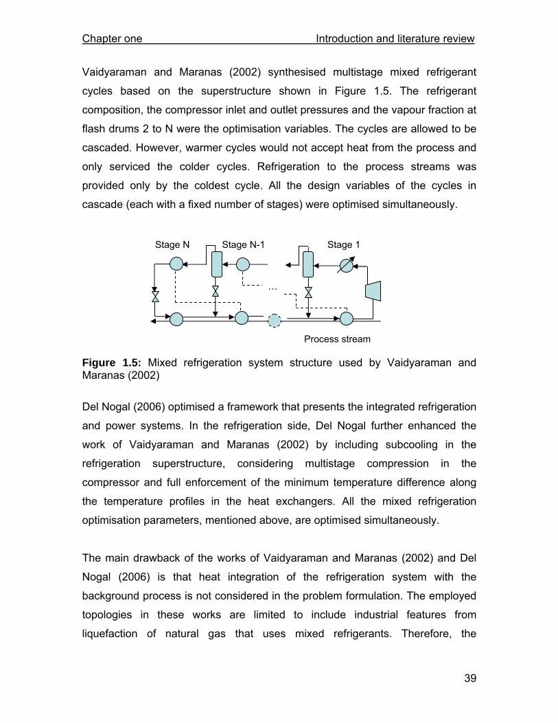
Chapter one Introduction and literature review
39
Vaidyaraman and Maranas (2002) synthesised multistage mixed refrigerant
cycles based on the superstructure shown in Figure 1.5. The refrigerant
composition, the compressor inlet and outlet pressures and the vapour fraction at
flash drums 2 to N were the optimisation variables. The cycles are allowed to be
cascaded. However, warmer cycles would not accept heat from the process and
only serviced the colder cycles. Refrigeration to the process streams was
provided only by the coldest cycle. All the design variables of the cycles in
cascade (each with a fixed number of stages) were optimised simultaneously.
Figure 1.5: Mixed refrigeration system structure used by Vaidyaraman and Maranas (2002)
Del Nogal (2006) optimised a framework that presents the integrated refrigeration
and power systems. In the refrigeration side, Del Nogal further enhanced the
work of Vaidyaraman and Maranas (2002) by including subcooling in the
refrigeration superstructure, considering multistage compression in the
compressor and full enforcement of the minimum temperature difference along
the temperature profiles in the heat exchangers. All the mixed refrigeration
optimisation parameters, mentioned above, are optimised simultaneously.
The main drawback of the works of Vaidyaraman and Maranas (2002) and Del
Nogal (2006) is that heat integration of the refrigeration system with the
background process is not considered in the problem formulation. The employed
topologies in these works are limited to include industrial features from
liquefaction of natural gas that uses mixed refrigerants. Therefore, the
Stage N Stage N-1 Stage 1
Process stream
…

Chapter one Introduction and literature review
40
superstructure lacks the features of refrigeration systems using pure refrigerants.
For instance, in these works the evaporation of the refrigerant occurs only at a
single pressure. Therefore, the superstructure does not generate a multistage
cycle in which each level operates at different pressures. The latter is common in
industrial configurations of the refrigeration systems using pure refrigerants.
1.6 Summary of ‘Heat integrated separation sequence’ literature review In section 1.5, literature on each of the elements, which form the systematic
optimisation problem for a heat integrated separation sequence, is presented. In
this section, the intention is to summarise the literature on design of heat
integrated separation sequence. A number of recent studies on heat integrated
separation sequences are revisited. The points of strength and shortcomings of
each work are clarified and the gaps, which the present work intends to fill, are
highlighted.
Yeomans and Grossmann (1999a, b and 2000a, b) systematically optimised a
heat integrated distillation sequence at above ambient condition. The work
develops mathematical models for state task network and state equipment
network using generalised disjunctive programming (Raman and Grossmann,
1994). These models are employed as two different representations of the
superstructure for the process systems (Yeomans and Grossmann, 1998). Both
rigorous (Yeomans and Grossmann, 2000a) and shortcut (Yeomans and
Grossmann, 2000b) models for column design are considered. Rigorous models
limit the applicability of the method to the simple sequencing problems. Heat
integration is taken into account by using pinch analysis; hence, the heat
exchanger network design is not addressed. In addition, the reboiler and
condenser streams are assumed isothermal. The process for preparing the feed
(e.g. preheating or changing the pressure) to the downstream unit (from
upstream equipment) is not considered. These assumptions lead to a problem
formulation and super-structure that is inherently incapable of generating the

Chapter one Introduction and literature review
41
optimum process. Finding the global optimum solution remains uncertain as
deterministic approach is employed.
Wang et al. (1998) developed an improved genetic algorithm to optimise the
heat-integrated separation sequence, which operates at above ambient. Only
simple distillation column is included in this work. A task-based superstructure is
employed. Operating pressures of the columns are optimised as continuous
variables. Heat integration is also considered. A matrix approach is adopted,
where each hot stream can exchange heat with each cold stream if it is
thermodynamically feasible. However, heat exchangers are only in parallel and
heat exchanger in series are not accounted for. A major drawback of this model
is that it ignores feed preparation process. The feed to each column is the same
as the output of the upstream column and the column feed quality is not
optimised. The saturation of the superheated or subcooled feed in the column will
be at the expense of the reboiler or condenser load, which uses utility at the
extreme temperatures.
Another approach for optimal design of heat integrated distillation sequences is
proposed by Fraga and Zilinskas (2003). A hybrid optimisation approach is
suggested in this work: the top optimisation level manipulates the separation unit
design parameters, using local search methods and the inner level solves the
heat exchanger network problem through an evolutionary stochastic optimiser.
Heat exchanger network allows heat exchangers in series but not in parallel. The
possible matches between the cold and hot streams are presented through a
matrix. No superstructure representation for the sequences is reported in this
work and it may be that a fixed sequence is optimised while also heat integrated.
In that case, the approach is a sequential method, which will not simultaneously
optimise the separation sequence and heat integration opportunities.
Wang et al. (2008) addressed the problem of heat-integrated complex distillation
systems using genetic programming optimisation tool, which is similar to genetic

Chapter one Introduction and literature review
42
algorithm. The separation sequencing problem accounts for separation of an N-
component mixture into N products. Moreover, Wang et al. (2008) is not
considering feed conditioning processes. Therefore, in order to avoid unrealistic
designs, limiting assumptions are made, such as constraining the columns to
produce only saturated liquid products. Obviously, the type of condenser and the
feed quality are not optimised and the method is not practical for application to
low temperature processes. Moreover, heat integration matches between the
reboilers and condensers are optimised randomly and it is not clear whether the
heat exchangers are in parallel or in series.
Wang (2004) tackled the problem of heat integrated distillation sequence for
synthesis and optimisation of low-temperature gas separation processes. A task-
based superstructure is used for the sequencing problem. Both simple and
complex distillation columns are considered. Operating pressure is a continuous
optimisation variable. However, as for feed conditioning process only the
compression work of the feed to the plant is accounted for. Moreover, the feed to
each column is limited to the saturation conditions and two-phase feed is not
allowed. In addition, the non-isothermal enthalpy change of some process
streams is not accounted for. The refrigeration system is heat integrated with the
separation sequence, but heuristics are used for considering heat integration: 1)
Lifting heat from sources to sinks with minimum temperature differences is
preferred; 2) providing refrigeration to heat source required at lower temperature
is preferred to be operated prior to providing to those at higher temperature. Only
pure refrigerants are taken into account. Moreover, the refrigeration system is not
optimised and the complexity of the refrigeration system structure is not
controlled. So, practicality of the generated designs cannot be guaranteed.
A more recent work on low temperature separation processes belongs to
Markowski et al. (2007). A sequential approach in the design of separation
system, refrigeration system and heat exchanger network has been adopted.
Pinch technology is used for design of heat exchanger network. The temperature

Chapter one Introduction and literature review
43
levels in the refrigeration system are optimised by minimising the difference
between the exergy flows in the refrigeration levels and in the rejection levels of
the refrigeration cycle. The refrigeration system is not integrated with the rest of
process.
In summary, the above discussions reveal that the literature is short of a robust
approach for design of heat integrated low temperature separation sequences
that: simultaneously optimises key design variables in the separation and
refrigeration systems; addresses the structural options in separation sequence,
refrigeration system and heat recovery network; considers the stream
conditioning process in the separation sequence; handles non-isothermal
process streams; systematically takes into account different heat integration
opportunities within the separation system and between the separation and
refrigeration systems; accommodates different refrigeration provision strategies;
considers both pure and mixed refrigeration systems; overcomes the challenges
of solving a highly nonlinear problem and generates practical designs for large
industrial problems.
Chapter two Separation sequence synthesis
44
2 Chapter Two Separation sequence synthesis
2.1 Introduction The targeted separation problem in this work assumes a number of components
to be separated into a predefined set of products. The objective is to provide a
synthesis framework for systematic screening of separation processes, which
use distillation columns, to determine the cost-effective separation scheme. In
this framework, all the possible sequences of simple and complex separation
devices and various operating conditions for these devices should be considered.
Effective screening of various separation processes for providing a robust design
in an industrial problem is a difficult task. The challenges of such screening
attempt can be attributed to the large number of design options. Considering the
complex separation configurations such as side-rectifier, side-stripper,
prefractionator, side-draw columns and their operating conditions increase the
complexity of the problem significantly. Complex columns reduce mixing losses,
using available vapour and liquid more effectively and improve separation
efficiencies (Tedder and Rudd, 1978; Glinos and Malone, 1984; Triantafyllou and
Smith, 1992). However, they have wider temperature differences between
condenser and reboiler, which introduces complicated trade-offs between the
quality and quantity of refrigeration energy.
Shah (1999) proposed a task based representation for generating separation
sequences. Adopting a task based representation enables the approach to
accommodate all the design options, such as the type of distillation devices. In
this methodology, the multi-component separation is defined with recovery
matrix, which allows the separation of an m-component mixture to n components
(m≥n) to be considered. Later, Wang (2004) applied the methodology of Shah
(1999) for featuring the separation problem and generating separation
sequences in low temperature processes. Wang (2004) employed stochastic

Chapter two Separation sequence synthesis
45
optimiser for screening among various separation sequences, different simple
and complex distillation columns and their operating conditions.
Even though the developed framework by Wang (2004) is a robust screening
approach, there are a number of key areas in the separation sequencing problem
that are not addressed by Wang (2004). These issues are mainly the manner in
which the feed quality to each distillation device is optimised and the way in
which the stream conditioning process is dealt with. Stream conditioning refers to
the process for delivering the feed to a device at the required temperature and
pressure from the upstream conditions or preparing the products at the required
temperature and pressure.
In the previous work, the feed quality to each separation device can be optimised
to be either a saturated liquid or saturated vapour. In this thesis, the feed quality
is optimised and can be saturated liquid, saturated vapour or a two-phase
stream. Moreover, stream conditioning was not fully accounted for in the previous
work. Wang (2004) only evaluated the cost of the compression work for the initial
feed in a single stage compressor. In the present work, the stream conditioning
process is fully simulated and accounted for in the overall evaluation of the
process. These modifications have been applied to Wang (2004) approach and
the resulting methodology has been used in this work for synthesising and
optimisation of the separation sequences.
In this chapter, the developed and adopted approaches regarding the following
sections in the separation sequence design problem are discussed:
• the adopted strategy for generating various separation sequences, (Shah,
1999; Wang, 2004);
• the adopted shortcut models for separation units, both simple and
complex distillation columns, (King, 1980; Glinos and Malone, 1985;
Triantafyllou and Smith, 1992; Carlberg and Westerberg, 1989a,b);

Chapter two Separation sequence synthesis
46
• the optimisation parameters in the sequencing problem (Wang, 2004);
• the approach for simulation and evaluation of the stream conditioning
process.
2.2 Separation sequence synthesis A separation problem can be represented using a recovery matrix (Shah, 1999).
In a recovery matrix, the rows are the components in the mixture, which are listed
in order of decreasing volatility, and the matrix columns are the products whose
normal boiling point increases from left to right. The matrix elements are
fractional recoveries of the components in each product. Table 2.1 illustrates a
matrix of 7 components to be separated into 5 products. Unlike methods that use
lumping or pseudo components for each product, the recovery matrix can
consider the multi-component nature of each product.
Table 2.1: Recovery matrix for a 7-component mixture to be separated into 5 products
Recovery fractions in product i Component
Feed
composition A B C D E
1 Methane 0.35 0.99 0.01
2 Ethylene 0.40 0.005 0.99 0.005
3 Ethane 0.07 0.005 0.99 0.005
4 Propylene 0.11 0.01 0.98 0.01
5 Propane 0.01 0.01 0.97 0.02
6 1,3-butadiene 0.03 0.02 0.98
7 n-butane 0.03 0.01 0.99
Flowrate-kmol/s 1.58 0.55 0.63 0.11 0.19 0.1
A separation sequence is the order in which the components of a mixture are
separated from one another through a number of separation units. Separation
sequences can be represented by separation tasks. Hendry and Hughes (1972)
introduced the concept of separation tasks. Separation tasks can be classified as
simple and hybrid tasks.

Chapter two Separation sequence synthesis
47
A simple task separation features a single feed and two products with one light
and one heavy key component. For a C-product separation problem, the total
number of simple tasks (TC) is given as:
6)1C(C)1C(TC
+⋅⋅=
- 2.1
Figure 2.1 shows the simple separation tasks for a five-product separation
problem. Twenty discrete simple tasks exist for the five-product separation. A
simple task can be implemented in the separation equipment, which is known as
a simple task representation. This equipment will have one feed and two
products. A simple distillation column is an example of this type of equipment.
A group of separation tasks from Figure 2.1 that are selected in a logical order
forms a separation sequence. Consider an illustrative example, where a
separation sequence can be obtained by linking tasks A/BCDE, B/CDE, C/DE
and D/E together, as shown in Figure 2.1. This separation sequence is called a
direct sequence. The characteristic of direct sequence is that at each stage of
separation, the light component is separated from the rest of components. On the
other hand, an indirect sequence is a sequence in which the heavy component is
separated at each separation device (Figure 2.1).
The flowchart in Appendix D shows the algorithm used in this work for generating
separation sequences consisting of only simple separation tasks. Two connected
simple tasks can be transformed into a hybrid task. A hybrid task features a
single feed and more than two products, with nonadjacent light and heavy key
components and is an ordered combination of simple distillation columns.

Chapter two Separation sequence synthesis
48
Figure 2.1: Simple tasks of a 5-product separation problem (Wang, 2004)
The number of possible hybrid tasks (HC) for an C-product system is given by the
following expression (Shah, 1999):
2.2
A hybrid task is carried out in a separation device, which is called hybrid task
representation. Several types of devices can handle hybrid tasks. Three types of
distillation hybrid task representations can be classified as follows:
• a single side-column arrangement, e.g. side-stripper column, side-rectifier
column, Figure 2.2 (a, b);
• a single product side-draw column, e.g. liquid side-draw column, vapour
side-draw column, Figure 2.2 (c, d);
• prefractionator arrangements: Prefractionator, Petlyuk column and
dividing-wall columns, Figure 2.2 (e, f, g).
Using recovery matrix for defining a separation problem, each separation task
representation can be simulated independent from its up- and down- stream
∑2C
1L
1LC
1KC K)-L-(CL H
−
=
−−
=⎥⎦⎤
⎢⎣⎡
⎟⎠⎞
⎜⎝⎛ ∑⋅=
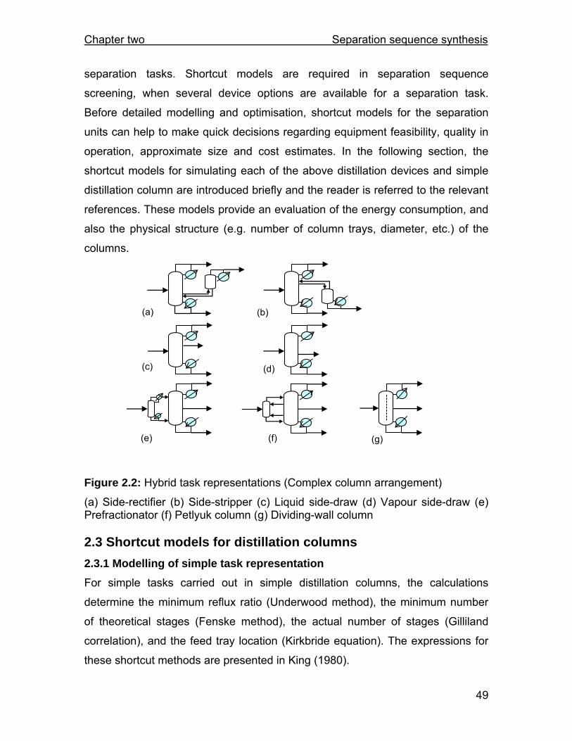
Chapter two Separation sequence synthesis
49
separation tasks. Shortcut models are required in separation sequence
screening, when several device options are available for a separation task.
Before detailed modelling and optimisation, shortcut models for the separation
units can help to make quick decisions regarding equipment feasibility, quality in
operation, approximate size and cost estimates. In the following section, the
shortcut models for simulating each of the above distillation devices and simple
distillation column are introduced briefly and the reader is referred to the relevant
references. These models provide an evaluation of the energy consumption, and
also the physical structure (e.g. number of column trays, diameter, etc.) of the
columns.
Figure 2.2: Hybrid task representations (Complex column arrangement) (a) Side-rectifier (b) Side-stripper (c) Liquid side-draw (d) Vapour side-draw (e) Prefractionator (f) Petlyuk column (g) Dividing-wall column 2.3 Shortcut models for distillation columns 2.3.1 Modelling of simple task representation For simple tasks carried out in simple distillation columns, the calculations
determine the minimum reflux ratio (Underwood method), the minimum number
of theoretical stages (Fenske method), the actual number of stages (Gilliland
correlation), and the feed tray location (Kirkbride equation). The expressions for
these shortcut methods are presented in King (1980).
(a) (b)
(c) (d)
(e) (f) (g)

Chapter two Separation sequence synthesis
50
2.3.2 Modelling of hybrid task representations In this work, accomplishments from a number of research groups for modelling
the hybrid task representations have been exploited (Glinos and Malone, 1985;
Triantafyllou and Smith, 1992; Carlberg and Westerberg, 1989a, b). These
models generally decompose the complex column arrangements into a number
of simple columns for evaluating the performance of the complex columns. In the
following sections, different complex columns together with their
thermodynamically equivalent arrangements are introduced and the reader is
referred to the relevant references for detailed discussions of the models.
2.3.2.1 Side-draw columns
Vapour side-draw columns can be modelled by combining a direct sequence of
separation tasks. If two separation tasks in the indirect sequence are merged, the
resulting hybrid separation task can be carried out in a liquid side-draw column.
Figure 2.3 shows the thermodynamic equivalent arrangements for the side-draw
columns. These arrangements consist of a simple distillation column and a
supplementary stripping section for vapour side-draw or a supplementary
rectifying section for the liquid side-draw column. The supplementary sections
are employed to separate the intermediate product (IP) from the light (LP) in the
liquid side-draw column or heavy (HP) product in the vapour side-draw column,
respectively. Only a limited degree of separation between IP and the other key
component (LP) in the liquid side-draw column or heavy (HP) product in the
vapour side-draw column) is possible, as only one column section is available for
their separation. Therefore, using the side draw column, one key component is
obtained as the column product with the specified purity and recovery in this
configuration and a fraction of the other non-intermediate key component is
carried over to the side-draw while some IP goes to the product carrying this key
component. Hence, the separation between IP and the HP (or LP) in the vapour
side-draw (or liquid side-draw column) is imperfect (Glinos and Malone, 1985).

Chapter two Separation sequence synthesis
51
Glinos and Malone (1985) provide the shortcut model for simulating the side-
draw columns. This shortcut model predicts the minimum fraction of the light or
heavy key component in the side stream when the reflux ratio (in the case of
vapour side-draw) or the boil-up ratio (in the case of liquid side-draw) is fixed.
Figure 2.3: Thermodynamically equivalent arrangements for side-draw column (a,b) vapour side-draw column; (c,d) liquid side-draw column
2.3.2.2 Side column
Two types of side columns, side-rectifier and side-stripper columns are shown in
Figures 2.4-5. A side-rectifier can be simulated as two columns in a thermally
coupled direct sequence. As shown in Figure 2.4, in the simulation model the first
column is a conventional column with a condenser and a partial reboiler. A partial
reboiler takes the liquid from the column and vaporises part of it to generate a
liquid and a vapour product in equilibrium with one another. The second column
will be modelled as a vapour side-draw column (Carlberg and Westerberg,
1989a, b). The vapour side-draw is taken at one stage below the feed stage. The
properties of the connecting streams between the two columns are evaluated by
vapour-liquid equilibrium and mass balance calculation around the partial
reboiler.
(a) (b)
(c) (d)
Feed
Feed
Feed
Feed
LP
IP
HP
LP
IP
HP
LP
IP
HP
LP
IP
HP
Supplementary
stripping section
Supplementary
rectifying section

Chapter two Separation sequence synthesis
52
A side-stripper, (Figure 2.5), can be modelled by two thermally coupled columns
in an indirect sequence. In this case, the first column is a conventional column
with a partial condenser and reboiler. The second column is simulated as a liquid
side-draw column. The liquid side-draw is taken at one stage above the feed
stage. The properties of the connecting streams between the two columns are
evaluated by vapour-liquid equilibrium and mass balance calculation around the
partial condenser. More detail on modelling strategy of side-stripper and side-
rectifier can be found in Carlberg and Westerberg (1989a, b).
Figure 2.4: Equivalent arrangement for side-rectifier
Figure 2.5: Equivalent arrangement for side-stripper
LP
Feed
LP IP
HP
Feed IP
HP
F’
W’
F’
W’
Feed
FeedIP
HP
HP
LP
IP
F’
W’
W’
F’
LP

Chapter two Separation sequence synthesis
53
2.3.2.3 Prefractionator arrangements
A prefractionator column, together with its thermally coupled configurations (i.e.
Petlyuk column and dividing wall column), form another group of complex
columns, Figure 2.2 (e, f, g).
In the prefractionator column, the light key product (LP) is separated from the
heavy Key product (HP) and all the intermediate products (IP) are distributed
between its top and the bottom products. The recovery of the IP in the distillate of
the prefractionator is a degree of freedom, which is varied to minimise the reflux
ratio in the prefractionator.
Figure 2.6: Equivalent arrangement for prefractionator column
A prefractionator column can be represented by a combination of three simple
distillation columns, as illustrated in Figure 2.6. Column 1 represents the
prefractionating column with a partial reboiler and condenser. Columns 2 and 3
represent the main column, which accepts the distillate and the bottom products
of the prefractionator as the feeds. Vapour flow in the bottom of column 2 is
equated with the vapour flow at the top of column 3 to model the thermal
integration of the two columns.
The Petlyuk column (also known as thermally coupled prefractionator) and the
dividing wall column are thermally coupled prefractionating configurations. To
simulate these columns, one simple column with a partial reboiler and a partial
condenser, and two side-draw columns are required. One of the side-draw
Feed
LP
IP
HP
2
LP
IP
HP
F’
IP
F’
F” F”
1 1
3

Chapter two Separation sequence synthesis
54
columns will be a vapour side-stream column and the other one is a liquid side-
stream column, as shown in Figure 2.7.
Figure 2.7: Equivalent arrangement for Petlyuk and dividing-wall columns
Detailed modelling strategy for prefractionator columns can be found in
Triantafyllou and Smith (1992).
2.3.3 Summary The task based approach adopted for generating the separation sequences
enables the framework to assess and evaluate each task representation
independently from the performance of the upstream or downstream units, using
the simulation methodologies that were referred to in section 2.3. Employing the
recovery matrix, the composition and the flowrate of the feed and product
streams are known for each task representation a priori and only depend on the
separation function of the particular task.
2.4 Optimisation parameters of the separation sequence Pressure of the column, the feed quality to the column and the type of condenser
are three important degrees of freedom in the design of a distillation column.
2.4.1 Pressure The operating pressure is an important degree of freedom for distillation
columns. Pressure affects the relative volatility and hence the difficulty of
separation of the components. Moreover, it affects the thermal properties of the
LP LP
HP
IP Feed
HP
IP
IP
F’
F
W’
W”
F’
F”
W
W”
Feed
Chapter two Separation sequence synthesis
55
column, i.e. the temperature range that the column is operating between reboiler
and condenser. The pressure of the column also affects the sizing of the column
(the diameter and the wall thickness of the column). These column
characteristics contribute directly to the operating and capital cost of the
distillation column. Moreover, the pressure influences the heat integration
opportunities with the background process (Smith, 2005).
Vacuum conditions in the distillation column should be avoided unless some
aspects of the separation problem require operation at vacuum conditions (e.g.
preventing thermal decomposition of material) (King, 1980). Operating at above
atmospheric pressures is also not desirable unless (King, 1980):
1. the pressure is increased to allow the use of cooling water for
condensation;
2. a refrigerated utility is required for the condenser and at a higher pressure
a cheaper refrigeration system can service the condenser;
3. heat integration can be achieved by operating the distillation columns at
different pressures.
This work optimises the pressure as a continuous variable with the lower bound
being the atmospheric pressure or above that. The upper bound is problem
dependent and is selected to be away from the critical pressure of the
components and within practical range in terms of the available utility for the
system.
2.4.2 Feed quality Another important parameter to be optimised is the feed quality. The difference
between the temperature of the feed to the column and the tray temperature
reduces the second-law efficiency (Seader and Henley, 1998). Normally
subcooled liquid or superheated feeds to the column are avoided. This is
because such streams will not participate in the separation process until they

Chapter two Separation sequence synthesis
56
become saturated. Saturating the feed in the column increases the load on the
reboiler or condenser. Supplying a partially vaporised feed may be a better
option. This is due to the provision of heating or cooling for the feed at a more
moderate temperature compared to the reboiler and condenser temperatures
and using a two-phase feed reduces the load on either reboiler or condenser. A
cheaper utility may be required for feed heating or cooling than in the main
reboiler or condenser and the operating cost may be reduced. Moreover, partially
vaporising the feed may result in a closer match between the feed vapour and
liquid compositions and the equilibrium compositions of the column feed stage.
In previous research (e.g. Wang, 2004; Wang et al., 2008), optimising the feed
quality was either not considered or it was limited to only saturated liquid and
vapour. Considering only these extreme conditions may restrain the optimiser
from finding the global optimum solution. In this work, feed quality is taken as a
continuous variable with the lower bound and upper bound being the saturated
liquid and saturated vapour; respectively.
2.4.3 Condenser type The type of the condenser (partial or total) is another optimisation parameter
considered in this work. By allowing the optimiser to choose the type of
condenser, the load on the condenser will be optimised by liquefying the top
product only when it is necessary or economical. The associated variable is a
discrete optimisation variable.
2.5 Stream conditioning 2.5.1 Feed conditioning: Stream or feed conditioning refers to implementing the process, which accepts a
stream from the upstream devices and changes its condition to match the
required pressure and quality of the feed to the downstream process. In a
separation sequence, stream conditioning is an important part of the process and
the design and costing of it should not be ignored in the conceptual design stage.

Chapter two Separation sequence synthesis
57
The operating and capital cost for the process of preparing the feed can change,
considerably and unfavourably, the economics of a specific design.
Let us consider the two separation sequences shown in the following illustrative
example that carry out the same separation task, shown in Table 2.2.The utility
cost of each design is summarised in Table 2.4. If feed conditioning is ignored
and the utility costs (of the reboilers, condensers and compression work) are not
included in the cost of the process, the operating cost (i.e. the utility costs of the
reboilers and condensers) of Design 1 in Figure 2.8 will be lower than Design 2 in
Figure 2.8 by 5%, as it requires less and cheaper refrigerated utility. Therefore, if
the separation sequences are screened based on the utility cost (without
accounting for the feed conditioning), Design 1 will be selected as the optimum.
However, in practice, Design 1 has a utility cost, which is 117% of the utility cost
in Design 2, when the cost of feed conditioning is also determined and included
in the overall utility cost. Therefore, Design 2 is the optimum option (with lower
utility cost) in between these two sequences. Obviously, this example illustrates
that considering the feed conditioning can change the economical order of the
separation sequences.
Illustrative example Table 2.2: Separation problem specifications
i Components in feed Mole fraction Product specification
1 Methane 0.35 99% recovery of methane
2 Ethylene 0.40 99% recovery of ethylene
3 Ethane 0.07
4 Propene 0.11
5 Propane 0.01
6 1,3 Butadiene 0.03
7 n-butane 0.03
99% recovery of ethane
Flowrate 5700 kmol/h, saturated vapour at 9 bar

Chapter two Separation sequence synthesis
58
Table 2.3: Utility specifications
Type Temperature (˚C) Cost index (US$/kW.yr)
hot utility
Hot water 90 82
Low-pressure steam 150 146
Medium-pressure steam 200 179
High-pressure steam 250 195
cold utility
Cooling water 30-45 24
Electric power (energy) 571.04
Figure 2.8: Two possible separation sequences for the problem in table 2.2
1
2
-126 °C 0.9 MW
-43 °C 8.5 MW
25.2 MW
-103 °C -55 °C 14 MW
0°C 22.1 MW
9 bar
9 bar
Utility cost excluding feed conditioning: 12.5 MM $ Utility cost including feed conditioning: 44.1 MM $ Design 2: Simulation carried out in HYSYS using shortcut model for distillation columns
-12 °C
C2H6+
C2H4
CH4
4 MW 1
2
25.4 MW
-69 °C
-47 °C 14 MW
44 °C 28.8 MW
-111 °C
13.5 MW
-126 °C 0.8 MW
-55 °C 6.4 MW
Utility cost excluding feed conditioning: 11.9 MM $ Utility cost including feed conditioning: 51.5 MM $
23bar
9 bar
Design 1: Simulation carried out in HYSYS using shortcut model for distillation columns
-12 °C
CH4
C2H4
C2H6+

Chapter two Separation sequence synthesis
59
Table 2.4: Operating costs for Designs 1 and 2 in Figure 2.8
Excluding feed conditioning
process (MM$/yr)
Including feed conditioning
process (MM$/yr)
Design 1 (A) 11.9 51.5
Design 2 (B) 12.5 44.1
Cost of A / Cost of B 95% 117%
The feed preparation process can create heat integration opportunities for the
rest of the process. Therefore, design and evaluation of the feed preparation
process has to be taken into account in parallel with the design of the rest of the
process, since it will directly affect the economics of the sequence.
To prepare the feed, the state of the feed stream should be changed from
upstream conditions (A) to the required downstream conditions (B). In other
words, the feed temperature, pressure or both may need to be changed through
a path consisting of compression, expansion, cooling or heating. The designer
needs to compare different feasible orders of compression, expansion, cooling
and heating in different phases for changing the state of feed from A to B.
From the energy point of view, the change is associated with an enthalpy
change. Enthalpy change of the feed stream is a state function, i.e.: the net
required energy for transforming feed from state A to state B will be the same
through all different feasible paths. However, in practice the quality of the
energies added to or rejected from the process and their quantities depends on
the path. Typically, the cost per unit energy of hot utility increases with its
temperature and that of cold utilities increases as its temperature decreases.
Therefore, a process, which avoids high temperature and/or low temperature
utilities, can prove more economical than a process with such temperatures.
Moreover, some process operations inherently demand more energy compared
to the others, such as compressing vapour compared to pumping the liquids. The
energy consumption of a device can also depend on the condition of the input

Chapter two Separation sequence synthesis
60
fluids. For example, less energy is required for compressing a cold gas
compared to a warmer gas.
For instance, suppose the optimiser chooses a saturated liquid feed for a
downstream column in a direct sequence where the downstream pressure is also
lower than the upstream pressure. More precisely, a column in a sequence
produces a saturated liquid product at pressure, P1, as the bottom product. This
product feeds the downstream column, which has been specified to operate at a
lower pressure, P2, with a saturated liquid feed. Figure 2.9 illustrates the scenario.
Figure 2.9: Providing a saturated liquid feed from a saturated liquid stream at a lower pressure
To achieve the desired feed condition, different paths are possible:
Path 1 Initially expanding the saturated liquid to the lower pressure and then
cooling the two-phase fluid produced to saturated condition, as shown in path
abc in Figure 2.10.
Path 2 Sub-cooling the high pressure liquid and then letting down the sub-cooled
liquid to the final pressure, so that saturated liquid is obtained (Path ab’c in
Figure 2.10).
Feed conditioning
process
P1
P2 Saturated liquid
at P1
Saturated liquid at P2
P1 > P2

Chapter two Separation sequence synthesis
61
Figure 2.10: Temperature-enthalpy diagram for expansion of a saturated liquid
In path 1, *expanding the saturated liquid from a high pressure (point a in Figure
2.10) to a lower pressure often generates a two-phase fluid (point b in Figure
2.10). To produce a saturated liquid (point c in Figure 2.10) from the two-phase
fluid (point b in Figure 2.10), condensation of the generated vapour and cooling
of the liquid is required.
The expansion will be carried out through an isenthalpic process in a Joule-
Thomson valve. A temperature drop in the mixture is expected. The temperature
drop is partly due to the evaporation of a portion of the liquid. To produce a
saturated liquid, the generated vapour should be liquefied at the lower
temperature and pressure. In a below ambient process, this will introduce the
need for a colder utility, which may require more expensive refrigeration system
compared to the cold utility at a warmer temperature.
Another possible path is to sub-cool the saturated liquid at the higher pressure
(point a in Figure 2.10 to point b’ in Figure 2.10) before expanding it to the final
* The shape of the temperature-enthalpy profiles is different for various components and mixtures. The state of a stream after expansion or compression depends on the shape of the diagram.
Lines of constant pressure
a
b’
c
T
H
P1
P2b
Chapter two Separation sequence synthesis
62
pressure. Cooling the liquid at the high pressure will be at a higher temperature;
hence, a cheaper refrigeration system may be needed, compared to path 1. In
the next step, the sub-cooled liquid (point b’ in Figure 2.10) is expanded to the
desired pressure (point c in Figure 2.10). As shown in the Figure 2.10, the
expansion of a sub-cooled liquid will produce less vapour compared to expanding
a saturated liquid or a two phase fluid. Therefore, the required duty at the lower
temperature will be smaller or none. Thus, the resulting process will be cheaper
from the energy point of view.
However, in an above ambient process, selecting the feed preparation process
for this state change may not change the economics of the process as much as
in the below ambient process. This is because providing cooling to an above
ambient process is usually cheap. If heat integration options are to be taken into
account, then providing cooling at high temperature will be a more promising
opportunity, as it provides a heat source at a higher temperature for the rest of
the process.
2.5.2 Considering feed conditioning in the separation sequencing problem All in all, the design and costing of stream conditioning processes should be
considered and evaluated in the design of the separation sequence, because it
affects the economics of the process. The feed conditioning process can incur
considerable operating and capital costs. At the same time, this part of the
process can present integration opportunities for the rest of the process.
The way in which the feed conditioning is considered and implemented in the
separation sequence optimisation problem is important. As discussed in the
previous section, feed conditioning plays a role in the economics of a sequence
and should be accounted for in the separation sequence optimisation problem.
However, optimising the feed conditioning process may not be the best option, as
this would expand the size of the optimisation problem significantly. Optimising
feed conditioning adds many time-consuming calculations, such as calculating
Chapter two Separation sequence synthesis
63
the physical properties of the streams. In addition, the significance of optimising
the feed conditioning process compared to the other optimisation variables in
separation sequence optimisation problem is lower. For instance, fine tuning the
feed quality to a separation device or the pressure of the column affects the
economics of the process more than optimising the details of the feed
preparation process.
In this study, design and integration of the feed conditioning process is fully
evaluated. A number of heuristic rules, based on the engineering judgement, are
considered in choosing the feed conditioning process:
• Compressing a fluid in vapour phase is more expensive than pumping the
fluid in liquid phase, both in terms of capital and operating cost.
• Providing utility at extreme temperatures (i.e. very cold or very hot
temperatures) is more expensive than at moderate temperatures.
• If heat recovery is to be considered, operating the hot process streams at
the warmer temperatures and the cold process streams at the lower
temperature may generate better heat integration opportunities.
Moreover, the present work is flexible in accepting the decision of the designer to
allow or exclude certain options. For instance, the designer may decide that
compressors are only allowed on the inlet feed to the plant or the products but
not for the intermediate streams. Especially when the operating cost of the
process is optimised, this flexibility feature allows the user to control the
complexity of the design. The approach employed in this work for considering
and evaluating the feed conditioning process in different scenarios is elaborated
in Appendix A.
2.5.3 Product conditioning The outlet product from a unit operation may not be at the required product
temperature and pressure. Moreover, the pressure required for the product at the

Chapter two Separation sequence synthesis
64
exit from the plant may not be the optimum operating pressure for the unit
operation. Hence, fixing the operating conditions of the unit to be at the specified
conditions for the product is not the best choice. The options for treating the
outlet product from the unit (to match the plant product condition) should be
explored to identify the trade-offs and develop the optimum flowsheet. Here, the
discussions presented for feed conditioning are valid for the product stream
treating. In this work, only variations in pressure and temperature for the product
stream are considered and the unit operations are responsible for generating the
product at the required composition.
2.6 Summary The first part of this chapter revisited the separations sequence synthesis
approach of Shah (1999) and Wang (2004). The methodology of Wang (2004) is
exploited in this work for simultaneous design and optimisation of the separation
and the refrigeration system.
In the second part of this chapter, the importance of simulation and evaluation of
stream conditioning in the screening of separation sequences is demonstrated
and the developed strategy for considering stream conditioning process is
introduced.
2.7 Nomenclature C Number of products in a separation problem
HC Total number of hybrid tasks
HP Heavy product
IP Intermediate product
LP Light product
TC Total number of simple tasks

Chapter three Heat integration model
65
3 Chapter Three Heat integration model
3.1 Introduction This thesis is being documented at a time of fluctuating energy prices. Avoiding
or reducing damage to the environment, caused by human activities, is also
another serious challenge for the society today. Protecting the environment in the
context of chemical processes translates to adopting process strategies with the
least negative impact on nature. In order to reduce the harm on the environment,
the importance of reducing the primary energy usage in energy consuming
processes is increasing.
Distillation is a highly energy intensive unit operation that depends on the utility
system for its operation. Heat integrating distillation systems can help to reduce
the primary energy consumption of these processes. Fortunately, both in stand
alone mode and in sequences, distillation columns present the designers and
operators with numerous opportunities for heat integration.
The purpose of this research is to present a methodology for design of heat
integrated low temperature distillation systems. It has been demonstrated, in the
literature (Wang, 2004) and will be shown later in this chapter, that if the process
is selected and then heat recovery options are applied, the optimal design may
be missed. Therefore, in the present methodology, we will consider heat
integration (HI) at the very early stages in addressing the separation sequence
synthesis problem.
This chapter introduces the heat integration model employed in this work for
considering heat recovery opportunities in a separation sequence. Initially, the
context, for which the model is developed, is discussed. The strategies of the
model are then justified for the required context. Subsequently, the model is
presented together with an illustrative example.
Chapter three Heat integration model
66
3.2 Context and objectives of the developed heat integration model The purpose for the present work is to develop a robust methodology for
synthesis and optimisation of energy-efficient distillation sequences. Elaboration
on the overall structure of the methodology will be discussed in Chapter 5 and
here a short description is presented in order to illustrate the role of the heat
recovery model. Stochastic optimisation is used to solve the separation
sequence synthesis problem. The stochastic optimisation framework generates a
separation sequence (together with its operating conditions) at each step of the
optimisation. A heat integration model is then required to evaluate the heat
recovery potential in the generated sequence. Hence, the heat integration model
optimises the heat exchanger network (HEN) for a set of streams with known
outlet and inlet temperatures and duties. After heat integrating the process, the
operating cost of the sequence is calculated and fed to the optimiser. The
optimisation framework produces another separation sequence and the above
procedure is repeated until the termination criterion is met.
The present work develops a methodology for synthesising heat integrated
separation sequence, which can be applied to two types of processes:
• processes operating at below ambient temperatures;
• processes operating at above ambient temperatures.
The main difference between these two processes is in their required utility
system. A below-ambient process requires refrigerated utility, while utility at
ambient temperatures can be used in the processes operating above the ambient
temperature. In a below-ambient process, it is desired to consider the integration
of the separation and refrigeration systems. These two systems interact through
the HEN. Hence, a heat recovery model is required that can accommodate and
consider these interactions.

Chapter three Heat integration model
67
It should be remembered that the objective is to screen separation sequences.
Separation sequence synthesis problem alone is a complex problem. The
amount of detail considered in the heat integration model should be chosen with
caution in order to control the complexity of the problem. The main role of the
HEN optimisation model in the sequencing problem is to identify the potential for
heat integration in any specific sequence and credit the sequence for these
opportunities.
The heat integration model should also limit its search space to practical designs.
For instance, too many small heat exchangers will not prove economical, even if
the least utility cost is associated with such designs. This is because the higher
capital and maintenance costs of this design make it an impractical option.
In this work, the heat integration approach proposed by Fraga and Zilinskas
(2003) and Wang et al. (1998) for design of heat integrated separation
sequences is adopted and modified to fulfil the objectives of the present work.
This heat integration approach explores all possible heat exchanges (i.e.
matches) between the sources and the sinks in the process. Different possible
matches are identified and explored. The possibilities are represented by a
matrix, in which the rows represent heat sources, the columns represent heat
sinks and the elements indicate the feasibility of a particular match. Fraga and
Zilinskas (2003) do not allow heat exchangers in parallel and Wang et al. (1998)
do not allow heat exchangers in series. In this work, both stream splitting and
heat exchangers in series are considered. In addition, the heat integration
opportunities with a possibly present refrigeration utility system are accounted
for.
3.3 Problem statement for the heat integration model The problem to be addressed can be stated as follows. The heat integration
model is provided with a set of cold (C) and hot (H) streams with known inlet and
outlet temperatures and duties. The temperature and unit costs for the
Chapter three Heat integration model
68
appropriate cold and hot utilities are also available. Cold utilities include the utility
at ambient temperature (e.g. cooling water) and a heat pump system. The heat
pump system is considered so that heat can also be transferred between sources
and sinks where the source is colder than the sink. Theoretically, the heat pump
system can absorb heat from any source in the process and reject the heat to
any sink that is available. A refrigeration system is an example of a heat pump
system. Steam at different pressure levels is assumed to be available. The
objective is to determine the optimum utility cost for the corresponding heat
exchanger network (HEN). In other words, it is desired to find the optimal duties
of the feasible matches (i.e. feasible heat exchanges) between the hot and the
cold streams such that the network features minimum utility cost. Including the
capital cost of the system in the objective function, so that the total annualised
cost is optimised, is proposed as part of future work in Chapter 8. The following
characteristics should be incorporated in the proposed model:
• The heat integration model should be able to consider integration with
refrigeration system. In other words hot streams should be able to reject
heat to the refrigeration system and cold stream should be able to absorb
heat from the refrigeration system.
• The heat integration model should be able to take into account practical
constraints. Such constraints may include the number of refrigerant fluids
or the number of compression stages in the heat pump system.
3.4 Characteristics of the developed heat integration model 3.4.1 HEN Framework As discussed in section 3.2, the objective is to develop a framework, which
considers the heat integration options between the streams of the separation
sequence. Moreover, at the same time, the framework should consider the heat
recovery opportunities between the streams of the separation process and the

Chapter three Heat integration model
69
background process (if it exists). In the present work, a refrigeration system may
be present as the background process.
Few works in literature have studied the simultaneous design of heat-integrated
low-temperature sequences. Wang (2004) optimised the low-temperature
separation sequences and considered the heat integration between the
separation sequence and the refrigeration system. However, Wang (2004)
applied heuristics to heat integrate the refrigeration system and the separation
sequence. The number of compression stages in the refrigeration system is not
controlled and hence, impractical designs with many compression stages are
generated by this method. If the constraint on the number of compression stages
would have been applied, heuristic rules could have contradicted each other.
Therefore, instead of heuristics, a systematic methodology is required in order to
avoid conflicting and misleading results.
There are a number of studies in literature that optimise the heat exchanger
network and the refrigeration system simultaneously, using systematic
approaches (Shelton and Grossmann, 1986a, b; Colmenares and Seider, 1989;
Wu and Zhu, 2002). These research works are not simultaneously optimising the
background process with the refrigeration system. In these studies, systematic
HEN design models, such as pinch and transshipment, are used. These methods
generate temperature intervals. First, the process streams present in each
temperature interval are heat integrated. Thereafter, the remainder of the heat
surplus or deficit (in each temperature interval) will only be available to exchange
heat systematically with the streams in other intervals. However, in certain
scenarios (as illustrated in the following illustrative example), it is economical to
integrate a process stream with the refrigeration system and not with another
process stream. Therefore, if some of the process streams are heat integrated,
prior to evaluating the option of integrating them with the refrigeration system, the
optimum solution may be missed. Hence, the heat integration in the separation

Chapter three Heat integration model
70
system and between the separation and the refrigeration processes should be
taken into account simultaneously.
Illustrative example 1 Figure 3.1 shows a direct sequence for the separation problem shown in Table
3.1. The condenser and the reboiler temperatures and duties are summarised in
Table 3.2.
Table 3.1: Separation problem specifications for illustrative example 1 i Components in feed Mole fraction Product specification
1 Ethylene 0.52
2 Ethane 0.25
99% recovery
of ethane
3 Propene 0.06
4 Propane 0.06
5 1,3 Butadiene 0.06
6 n-butane 0.05
99% recovery
of propane
Flowrate 3600 kmol/h, saturated liquid at 2 bar
Figure 3.1: Separation sequence flowsheet
Simulation carried out in HYSYS
1
2
2 bar
8 bar

Chapter three Heat integration model
71
Table 3.2: Thermal specifications of the separation sequence in Figure 3.1
Units T (°C) Load (MW)
Column 1 Condenser -87 11.5
Column 2 Condenser 13.9 3.7
Column 1 Reboiler -14 12.7
Column 2 Reboiler 65 5.2
Two scenarios are considered. In scenario one, integration of the refrigeration
system with the separation sequence is accounted for after the sequence is heat
integrated. Figure 3.2 shows the balanced grand composite curve for this
scenario. In this scenario, the condenser of column 2 is integrated with the
reboiler of column 1. The refrigeration system is also rejecting heat to the reboiler
of column 1. The shaft power requirement for this flowsheet is 17.8 MW.
Figure 3.2: Balanced Grand Composite Curve for scenario one
In the second scenario, the integration of the separation system is considered
simultaneously with the integration of refrigeration and separation systems.
Figure 3.3 shows the balanced grand composite curve for this scenario. Here,
the reboiler of column 1 is fully integrated with the refrigeration system (instead of
Condenser of column 2 integrated with
the reboiler of column 1.
T (°C)
H (MW)0
-87
-47
-14
14
65
11.5
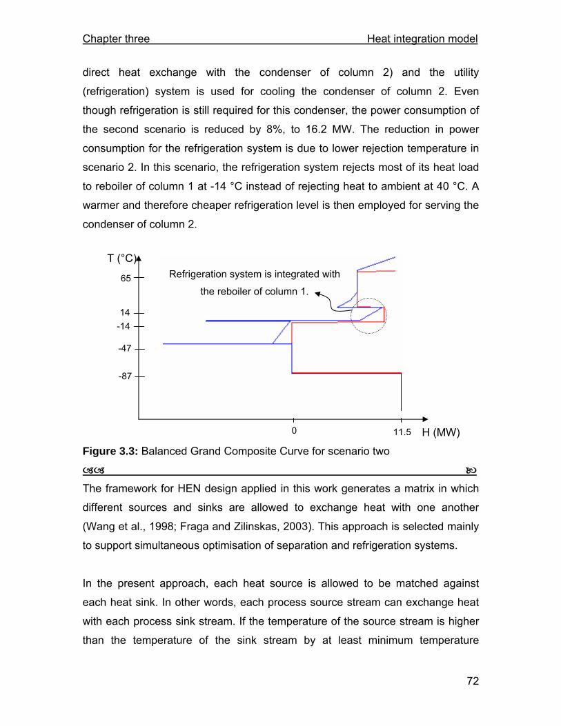
Chapter three Heat integration model
72
direct heat exchange with the condenser of column 2) and the utility
(refrigeration) system is used for cooling the condenser of column 2. Even
though refrigeration is still required for this condenser, the power consumption of
the second scenario is reduced by 8%, to 16.2 MW. The reduction in power
consumption for the refrigeration system is due to lower rejection temperature in
scenario 2. In this scenario, the refrigeration system rejects most of its heat load
to reboiler of column 1 at -14 °C instead of rejecting heat to ambient at 40 °C. A
warmer and therefore cheaper refrigeration level is then employed for serving the
condenser of column 2.
Figure 3.3: Balanced Grand Composite Curve for scenario two
The framework for HEN design applied in this work generates a matrix in which
different sources and sinks are allowed to exchange heat with one another
(Wang et al., 1998; Fraga and Zilinskas, 2003). This approach is selected mainly
to support simultaneous optimisation of separation and refrigeration systems.
In the present approach, each heat source is allowed to be matched against
each heat sink. In other words, each process source stream can exchange heat
with each process sink stream. If the temperature of the source stream is higher
than the temperature of the sink stream by at least minimum temperature
Refrigeration system is integrated with
the reboiler of column 1.
T (°C)
-87
-47
-14
65
14
H (MW)0 11.5

Chapter three Heat integration model
73
approach, the two streams can exchange heat directly. Otherwise, an external
heat pump system will be employed to absorb heat from the source stream and
reject it to the sink stream. It should be noted that the heat pump system (i.e. the
refrigeration system) will have the chance to reject heat to all of the process sinks
and hence, its integration with the process is fully considered. Therefore, the
promising structure can be captured in the solution space.
3.4.2 Non-isothermal Streams A non-isothermal stream is a stream that releases or gains heat over a
temperature range. Another feature of this model is that non-isothermal streams
are not considered isothermal. In some heat recovery methodologies (e.g.
Samanta, 2001 and Wang and Smith, 2005) the heat is provided or extracted
from a stream at the target temperature of the stream. This class of approaches
reduces some of the heat integration opportunities. For instance, Figure 3.4-(a)
shows a process source and a process sink. The process source needs to be
cooled down from 50˚C to 20˚C. The sink stream is absorbing heat at 25 ˚C. If all
the heat is to be absorbed from the source at the target temperature of 20 ˚C, the
heat exchange between these two streams will not be feasible (Figure 3.4-a)
and, an opportunity for heat integration will be missed. However, when the
temperature-enthalpy profile of the source streams is accounted for, the sink
stream can absorb part of the heat from the source stream (Figure 3.4-b).
Figure 3.4: T-H curves for heat transfer from a non-isothermal source stream
Supply Temperature
Target Temperature
Heat transfer
20
25
50
T ˚C
Ha
Supply Temperature
Target Temperature 20
25
50
T ˚C
H
DTmin =10 ˚C
35
b

Chapter three Heat integration model
74
In this work, the temperature change of a non-isothermal stream is taken into
account in heat integration. Inequalities 3.1 and Figure 3.5 illustrate the
approach.
Figure 3.5: Minimum temperature approach enforced both at inlet and outlet of source and sink streams
DT1 = Tout, source - Tin, sink > DTmin
Direct HI is feasible if & 3.1
DT2 = Tin, source - Tout, sink > DTmin
where Tin, source and Tout, source are the inlet and outlet temperatures of the process
source stream. Tin, sink and Tout, sink are the inlet and outlet temperatures of the
process sink stream.
Moreover, in this work, if a stream is exchanging both sensible and latent heat,
the stream is represented by two segments. For instance, let us consider the
scenario in which the outlet of a compressor (that is a superheated stream) is
condensed to a saturated liquid. This stream should first be de-superheated and
lose the sensible heat. The de-superheating step forms one process stream
segment in the temperature-enthalpy profile (segment a-b in Figure 3.6). Next,
the saturated vapour will be liquefied, releasing the latent heat (segment b-c in
Figure 3.6). This stage will be the second segment of the stream. Usually, the T-
H curves for these two parts have very different slopes. If liquefying of the
DT2
T
H
DT1

Chapter three Heat integration model
75
superheated vapour is considered in one stream segment such as segment a-c
in Figure 3.6 (neglecting the change in the slope of the T-H curves), infeasible
matches may be created between this stream and the process sink streams (e.g.
stream d-e), when heat integration is considered. Temperature cross may occur
since the minimum temperature approach is enforced only at the inlet and outlet
of the source and sink streams.
Figure 3.6: Illustration of a stream with both latent and sensible cooling
3.5 HEN design model description As discussed in section 3.2, the stochastic optimiser generates a separation
sequence at each step of the optimisation. Then the HEN for this fixed separation
sequence should be designed and optimised.
In this section, the HI approach employed will be explained through an illustrative
example.
• First the set of cold (C) and hot (H) streams is extracted from the
separation sequence.
C = {Ci |i = 1, n sink}
H = {Hj |j = 1, n source}
T
H
a
bc
Temperature cross
d
e
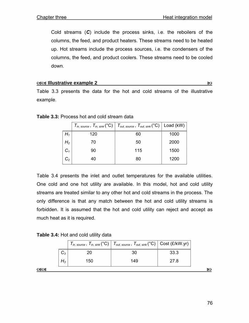
Chapter three Heat integration model
76
Cold streams (C) include the process sinks, i.e. the reboilers of the
columns, the feed, and product heaters. These streams need to be heated
up. Hot streams include the process sources, i.e. the condensers of the
columns, the feed, and product coolers. These streams need to be cooled
down.
Illustrative example 2 Table 3.3 presents the data for the hot and cold streams of the illustrative
example.
Table 3.3: Process hot and cold stream data
Tin, source , Tin, sink (°C) Tout, source , Tout, sink (°C) Load (kW)
H1 120 60 1000
H2 70 50 2000
C1 90 115 1500
C2 40 80 1200
Table 3.4 presents the inlet and outlet temperatures for the available utilities.
One cold and one hot utility are available. In this model, hot and cold utility
streams are treated similar to any other hot and cold streams in the process. The
only difference is that any match between the hot and cold utility streams is
forbidden. It is assumed that the hot and cold utility can reject and accept as
much heat as it is required.
Table 3.4: Hot and cold utility data
Tin, source , Tin, sink (°C) Tout, source , Tout, sink (°C) Cost (£/kW.yr)
C3 20 30 33.3
H3 150 149 27.8

Chapter three Heat integration model
77
• In the next step, the temperature range, covered by all the streams in the
cold (C) and hot (H) stream sets, is partitioned into temperature intervals
based on the Problem Table Algorithm (Linnhoff and Flower, 1978). The
main reason for generating the temperature intervals is to allow for heat
exchangers in series. Allowing heat exchangers in series permits
capturing the maximum heat recovery feasible among the process
streams. For instance, the streams presented in Figure 3.7(a) cannot be
heat integrated (assuming a hypothetical 0 ˚C minimum approach
temperature), unless the source and the sink stream are partitioned into
two segments.
Figure 3.7: T-H curves for a pair of crossing process source and sink streams
However, if the source and sink streams are partitioned into two stream
segments, as shown in Figure 3.7(b), part of the source stream can be
integrated with part of the sink stream in heat exchanger AA, as shown in
Figure 3.8. The source stream can be cooled down to the target
temperature in heat exchanger BB, which is in series with heat exchanger
AA.
Temperature crossT
H
T
H
Heat transfer is infeasible.
Hot stream
Cold stream
Hot stream
Cold stream
a) b)

Chapter three Heat integration model
78
Figure 3.8: HEN structure for the source and sink streams in Figure 3.7
It should be highlighted that in the present work the stream splitting is
permitted, but non-isothermal mixing of the streams are not considered.
The intermediate temperatures of the heat exchangers in series are not
optimised. This is in order to avoid complex heat recovery network design
problem. It should be remembered that the objective of the HEN design in
this work is to identify the opportunities for heat integration in the
separation sequence and with the background process. Therefore, a
detailed design of HEN is not pursued.
Note: The entire temperature range that all process streams cover
can be partitioned into temperature intervals according to the rules
proposed by Linnhoff and Flower (1978), Grimes et al. (1982), and
Cerda et al. (1983). However, it is important to ensure that a
dividing temperature exists in the temperature intervals at ambient
temperature. This dividing temperature is used to divide a stream,
which is partly operating at above ambient temperature and part of
it is at below ambient temperature, into two segments: one segment
operating fully at above ambient temperature and the second
segment is at below ambient temperature. Streams should be
partitioned at ambient temperature for two reasons. First reason is
to be able to apply the appropriate minimum approach temperature
(Dtmin), in case the user chooses different Dtmin for below and above
ambient streams. Generally, in industry smaller Dtmin is allocated in
B
AA
CC
Cold stream
Hot stream

Chapter three Heat integration model
79
heat exchangers operating at below ambient compared to the
above ambient heat exchangers. Lower Dtmin reduces the power
demand in the refrigeration system.
The second reason is that if a stream is covering a temperature
range, which is partly below ambient and partly above ambient, it is
expected that the optimum utility at each part would be a different
one. For example, if a stream is to be cooled down from 90 °C to -
30 °C with a total heat capacity flowrate, CP, of 10 kW/K (which is
the product of molar flowrate, m, and molar heat capacity, Cp, i.e.
CP=m·Cp), one should make sure that the stream is at least
partitioned into two streams, with the dividing temperature being
ambient plus Dtmin (e.g. 35 °C when ambient is at 25 °C and Dtmin at
above ambient temperature is 10°C). The reason is that, in case
this stream is to be cooled down in one segment, 1.2 MW of
refrigeration utility is required at a temperature, which should be
less than or equal -30 °C plus Dtmin at below ambient. However, if
the stream is divided at ambient, the refrigeration requirement can
be reduced by 0.55 MW, leaving this duty for the (cheaper) ambient
utility.
Therefore, the results of this step are the temperature intervals that later
will be used to partition the process streams.
Illustrative example 2 In this example, a uniform minimum temperature approach (Dtmin) of 10 °C is
assumed. In order to generate the temperature intervals, the inlet and outlet
temperatures of the hot and cold process streams are collected. Cold stream
temperatures will be shifted up in temperature by 21 ·Dtmin and hot streams will be
shifted down by 21 ·Dtmin. Shifting the temperature guarantees feasible heat
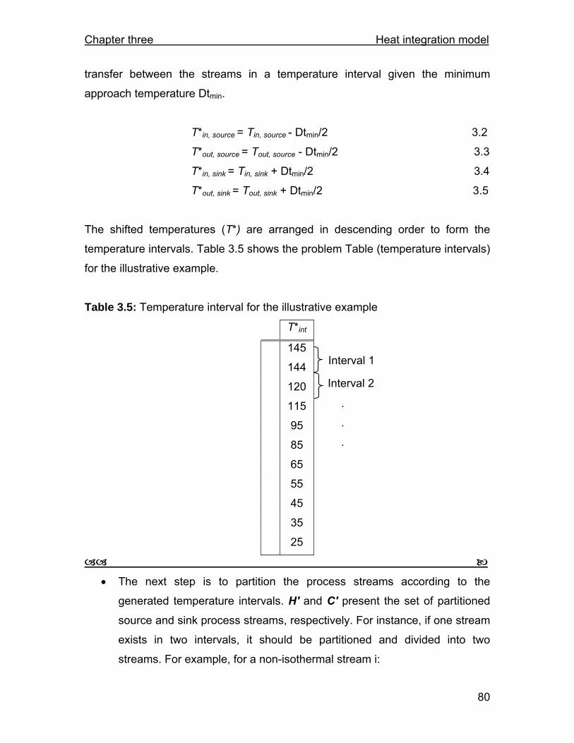
Chapter three Heat integration model
80
transfer between the streams in a temperature interval given the minimum
approach temperature Dtmin.
T*in, source = Tin, source - Dtmin/2 3.2
T*out, source = Tout, source - Dtmin/2 3.3
T*in, sink = Tin, sink + Dtmin/2 3.4
T*out, sink = Tout, sink + Dtmin/2 3.5
The shifted temperatures (T*) are arranged in descending order to form the
temperature intervals. Table 3.5 shows the problem Table (temperature intervals)
for the illustrative example.
Table 3.5: Temperature interval for the illustrative example
T*int
145
144
120
115
95
85
65
55
45
35
25
• The next step is to partition the process streams according to the
generated temperature intervals. H′ and C′ present the set of partitioned
source and sink process streams, respectively. For instance, if one stream
exists in two intervals, it should be partitioned and divided into two
streams. For example, for a non-isothermal stream i:
Interval 2
.
.
.
Interval 1

Chapter three Heat integration model
81
)T'- (T' · CP LD' k 1kki += 3.6
where kiLD' is the heat load, and T′ k+1 and T′k are the shifted outlet and
inlet temperatures of segment k belonging to the process stream i. In
addition, CP is:
CP = LD / (Tout - Tin) 3.7
LD is the heating or cooling demand of the stream. An isothermal stream
will not be partitioned.
As it was mentioned before, the reason for partitioning process streams is
to allow heat exchangers in series as well as in parallel. Obviously, the
intermediate temperatures of the heat exchangers in series are not
optimised. The intermediate temperatures are limited to the inlet and outlet
temperatures of the existing process streams and utilities.
Illustrative example 2 Table 3.6 presents the partitioned hot and cold process streams.
Table 3.6: Partitioned hot and cold streams
T′in, sink (°C) T′out, sink (°C) LD' ki (KW)
11'C 110 115 300
21'C 90 110 1200
32'C 60 80 600
42'C 50 60 300
52'C 40 50 300
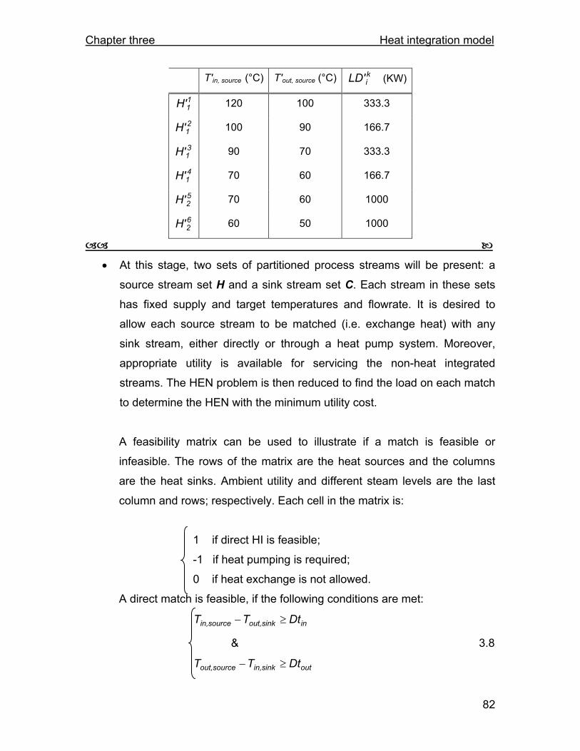
Chapter three Heat integration model
82
T′in, source (°C) T′out, source (°C) LD' ki (KW)
11'H 120 100 333.3
21'H 100 90 166.7
31'H 90 70 333.3
41'H 70 60 166.7
52'H 70 60 1000
62'H 60 50 1000
• At this stage, two sets of partitioned process streams will be present: a
source stream set H and a sink stream set C. Each stream in these sets
has fixed supply and target temperatures and flowrate. It is desired to
allow each source stream to be matched (i.e. exchange heat) with any
sink stream, either directly or through a heat pump system. Moreover,
appropriate utility is available for servicing the non-heat integrated
streams. The HEN problem is then reduced to find the load on each match
to determine the HEN with the minimum utility cost.
A feasibility matrix can be used to illustrate if a match is feasible or
infeasible. The rows of the matrix are the heat sources and the columns
are the heat sinks. Ambient utility and different steam levels are the last
column and rows; respectively. Each cell in the matrix is:
1 if direct HI is feasible;
-1 if heat pumping is required;
0 if heat exchange is not allowed.
A direct match is feasible, if the following conditions are met:
insinkout,sourcein, DtTT ≥−
& 3.8
outsinkin,sourceout, DtTT ≥−
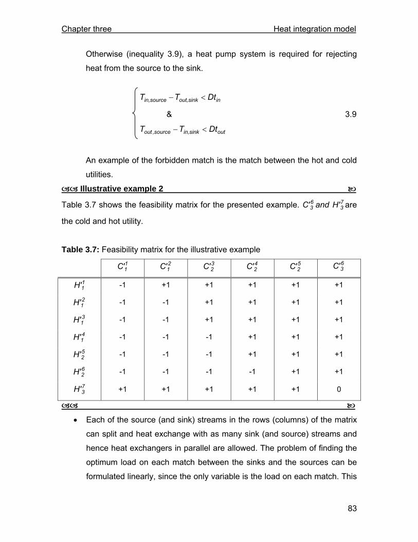
Chapter three Heat integration model
83
Otherwise (inequality 3.9), a heat pump system is required for rejecting
heat from the source to the sink.
insinkout,sourcein, DtTT <−
& 3.9
outsinkin,source,out DtTT <−
An example of the forbidden match is the match between the hot and cold
utilities.
Illustrative example 2
Table 3.7 shows the feasibility matrix for the presented example. 63'C and 7
3'H are
the cold and hot utility.
Table 3.7: Feasibility matrix for the illustrative example
11'C 2
1'C 32'C 4
2'C 52'C 6
3'C
11'H -1 +1 +1 +1 +1 +1
21'H -1 -1 +1 +1 +1 +1
31'H -1 -1 +1 +1 +1 +1
41'H -1 -1 -1 +1 +1 +1
52'H -1 -1 -1 +1 +1 +1
62'H -1 -1 -1 -1 +1 +1
73'H +1 +1 +1 +1 +1 0
• Each of the source (and sink) streams in the rows (columns) of the matrix
can split and heat exchange with as many sink (and source) streams and
hence heat exchangers in parallel are allowed. The problem of finding the
optimum load on each match between the sinks and the sources can be
formulated linearly, since the only variable is the load on each match. This
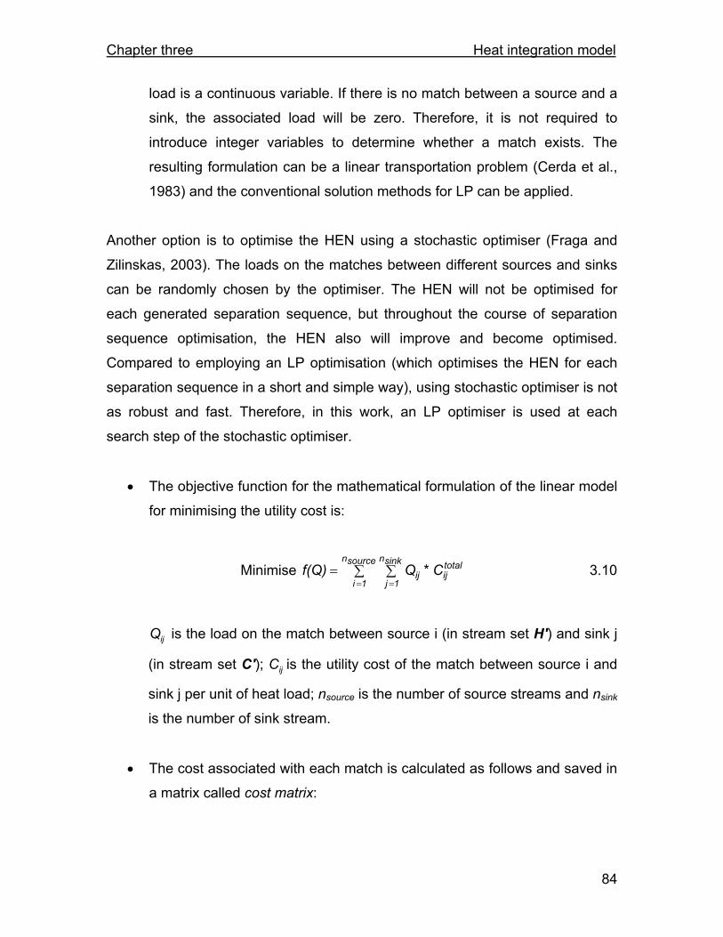
Chapter three Heat integration model
84
load is a continuous variable. If there is no match between a source and a
sink, the associated load will be zero. Therefore, it is not required to
introduce integer variables to determine whether a match exists. The
resulting formulation can be a linear transportation problem (Cerda et al.,
1983) and the conventional solution methods for LP can be applied.
Another option is to optimise the HEN using a stochastic optimiser (Fraga and
Zilinskas, 2003). The loads on the matches between different sources and sinks
can be randomly chosen by the optimiser. The HEN will not be optimised for
each generated separation sequence, but throughout the course of separation
sequence optimisation, the HEN also will improve and become optimised.
Compared to employing an LP optimisation (which optimises the HEN for each
separation sequence in a short and simple way), using stochastic optimiser is not
as robust and fast. Therefore, in this work, an LP optimiser is used at each
search step of the stochastic optimiser.
• The objective function for the mathematical formulation of the linear model
for minimising the utility cost is:
Minimise ∑ ∑== =
sourcen
1i
sinkn
1j
totalijij C*Qf(Q) 3.10
ijQ is the load on the match between source i (in stream set H′) and sink j
(in stream set C′); ijC is the utility cost of the match between source i and
sink j per unit of heat load; nsource is the number of source streams and nsink
is the number of sink stream.
• The cost associated with each match is calculated as follows and saved in
a matrix called cost matrix:
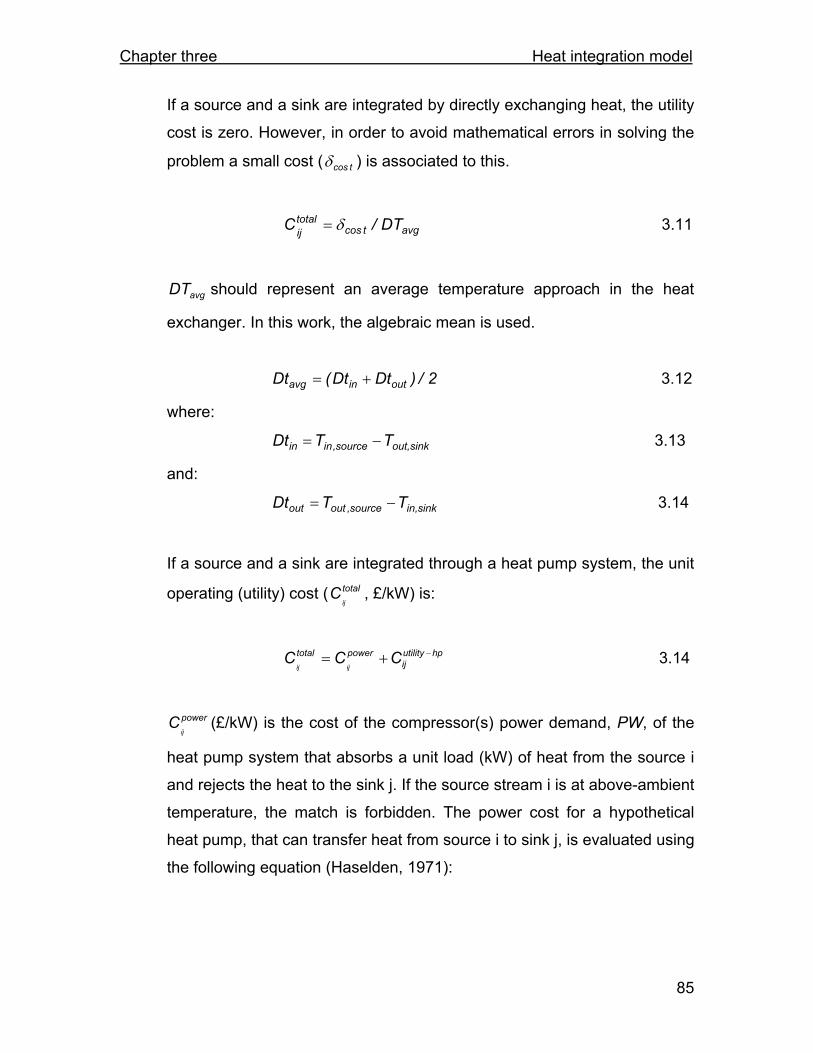
Chapter three Heat integration model
85
If a source and a sink are integrated by directly exchanging heat, the utility
cost is zero. However, in order to avoid mathematical errors in solving the
problem a small cost ( tcosδ ) is associated to this.
avgtcostotalij DT/C δ= 3.11
avgDT should represent an average temperature approach in the heat
exchanger. In this work, the algebraic mean is used.
2/)DtDt(Dt outinavg += 3.12
where:
sinkout,source,inin TTDt −= 3.13
and:
sinkin,source,outout TTDt −= 3.14
If a source and a sink are integrated through a heat pump system, the unit
operating (utility) cost ( totalij
C , £/kW) is:
hputility
ijpowertotal CCCijij
−+= 3.14
powerij
C (£/kW) is the cost of the compressor(s) power demand, PW, of the
heat pump system that absorbs a unit load (kW) of heat from the source i
and rejects the heat to the sink j. If the source stream i is at above-ambient
temperature, the match is forbidden. The power cost for a hypothetical
heat pump, that can transfer heat from source i to sink j, is evaluated using
the following equation (Haselden, 1971):
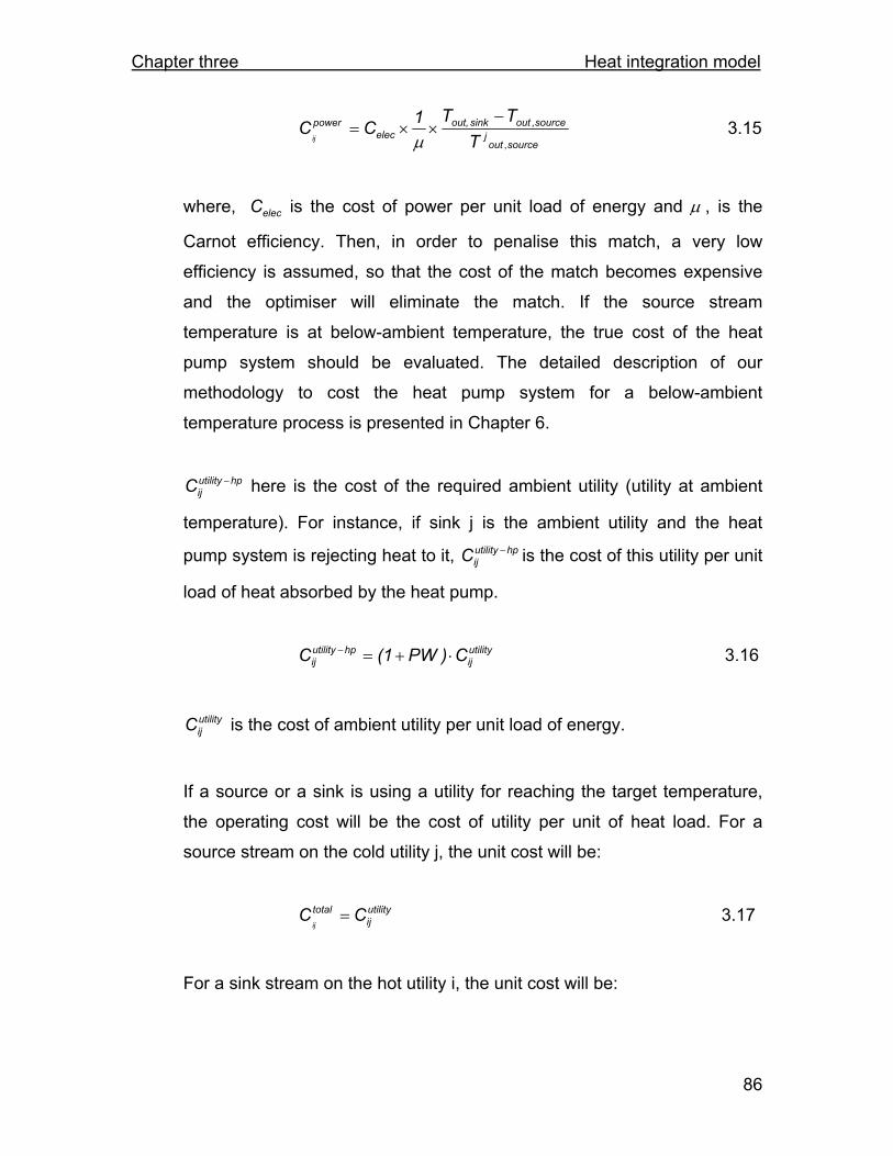
Chapter three Heat integration model
86
source,outj
source,outsink out,elec
power
TTT1CC
ij
−××=
μ 3.15
where, elecC is the cost of power per unit load of energy and μ , is the
Carnot efficiency. Then, in order to penalise this match, a very low
efficiency is assumed, so that the cost of the match becomes expensive
and the optimiser will eliminate the match. If the source stream
temperature is at below-ambient temperature, the true cost of the heat
pump system should be evaluated. The detailed description of our
methodology to cost the heat pump system for a below-ambient
temperature process is presented in Chapter 6.
hputility
ijC − here is the cost of the required ambient utility (utility at ambient
temperature). For instance, if sink j is the ambient utility and the heat
pump system is rejecting heat to it, hputilityijC − is the cost of this utility per unit
load of heat absorbed by the heat pump.
utilityij
hputilityij C)PW1(C ⋅+=− 3.16
utilityijC is the cost of ambient utility per unit load of energy.
If a source or a sink is using a utility for reaching the target temperature,
the operating cost will be the cost of utility per unit of heat load. For a
source stream on the cold utility j, the unit cost will be:
utilityij
total CCij
= 3.17
For a sink stream on the hot utility i, the unit cost will be:

Chapter three Heat integration model
87
utilityij
total CCij
= 3.18
Illustrative example 2
Table 3.8 shows the cost matrix for the illustrative example. tcosδ is taken to be
10-3 £. HP stands for the unit cost of heat pump shaft work. The calculation
procedure for the heat pump shaft work will be expanded in Chapter 6.
Table 3.8: Cost matrix for the illustrative example
11'C 2
1'C 32'C 4
2'C 52'C 6
3'C
11'H HP 10-4 2.5·10-5 1.8·10-5 1.5·10-5 27.8
21'H HP HP 4·10-5 2.5·10-5 2.5·10-5 27.8
31'H HP HP 10-4 4·10-5 2.9·10-5 27.8
41'H HP HP HP 10-4 5·10-5 27.8
52'H HP HP HP 10-4 5·10-5 27.8
62'H HP HP HP HP 10-4 27.8
73'H 33.3 33.3 33.3 33.3 33.3 61.1
• Energy balances are the equality constraints of this objective function.
Energy balance equations are needed to ensure that each stream is
heated or cooled enough to reach its target temperature. These equality
constraints specify that heat transferred to (from) each cold (hot) stream
must be equal to the sum of its heat exchanges with the cold (hot)
streams. It should be remembered that hot and cold utilities are also a
number of hot and cold streams in this formulation.
For each partitioned source stream k belonging source stream i with
duty ki LD' :
∑== ksinn,1j
kjki Q LD' 3.19
Chapter three Heat integration model
88
kjQ is the load exchanged between source k and sink j.
For each partitioned sink stream k belonging sink stream j with duty
LD' kj :
∑== source1,ni
ikkj Q LD' 3.20
ikQ is the load exchanged between sink i and source k.
• Upper and lower bounds for the variables ijQ are set through inequality
constraints. The energy balances are employed for determining the
boundaries.
The lower bound to each match is 0.
0Qij ≥ 3.21
The upper bound for the match between the process source stream i and
the process sink stream j is the minimum load of i and j which is available
to reject by source or absorb by the sink.
For the source process stream i and the sink process stream j:
) LD', LD'min(Q kj
kiij ≤ 3.22
The upper bound for the match between the process source (sink) stream
i (j) and the relevant utility is equal to the process source (sink) load.
For the process source stream i matched against utility j:

Chapter three Heat integration model
89
kiij LD'Q ≤ 3.23
For the process sink stream j matched against utility i:
kjij LD'Q ≤ 3.24
The upper bound for the match between the cold and hot utility is 0. That
is no heat exchange is allowed between the utilities. For a hot utility i and
a cold utility j:
0Qij ≤ 3.25
Illustrative example 2
The upper bound for the variable ijQ is shown in Table 3.9 The upper bound for
the match between 63'C and 7
3'H is 0 to ban the match between these two utilities.
Table 3.9: The upper bounds for the heat load variables
11'C 2
1'C 32'C 4
2'C 52'C 6
3'C
11'H 300 333.3 333.3 300 300 333.3
21'H 166.7 166.7 166.7 166.7 166.7 166.7
31'H 300 333.3 333.3 300 300 333.3
41'H 166.7 166.7 166.7 166.7 166.7 166.7
52'H 300 1000 600 300 300 1000
62'H 300 1000 600 300 300 1000
73'H 300 1200 600 300 300 0
Carrying out the LP optimisation to minimise the objective function 3.10, subject
to the constraints 3.19-25, for the presented illustrative example generates the

Chapter three Heat integration model
90
heat exchanger network shown in Table 3.10 and Figure 3.9. In this design, the
source stream C2 is heat integrated with the present sink streams H1 and H2
through parallel and series heat exchangers. Utility is employed for satisfying the
remainder of cooling and heating demand of the streams.
Table 3.10: The optimised heat loads for the illustrative example
11'C 2
1'C 32'C 4
2'C 52'C 6
3'C
11'H 0 0 333.3 0 0 0
21'H 0 0 166.7 0 0 0
31'H 0 0 0 300 33.3 0
41'H 0 0 0 0 0 166.69
52'H 0 0 0 0 266.7 733.3
62'H 0 0 0 0 0 1000
73'H 300 1200 100 0 0 0
Figure 3.9: The optimised heat exchanger network for the illustrative example
3.6 Summary A robust model for designing the heat exchanger network of a fully heat
integrated process is presented in this chapter and its application is illustrated
C2
C1
H1
H2

Chapter three Heat integration model
91
with an above ambient temperature example. Even though the model in theory
can be applied to any process both below and above ambient temperatures, the
incentive in the present work is to exploit the capacity of the approach for
simultaneous design and optimisation of a low-temperature separation sequence
and refrigeration systems. This methodology is capable of fully accounting for
interaction between different parts of the process through the HEN by using a
matrix based approach.
In addition, it is demonstrated that the developed methodology can consider
stream splitting and series heat exchangers. Moreover, in this model non-
isothermal streams are not considered isothermal. These last two features
enable the present approach to capture the heat integration opportunity in the
process effectively.
Moreover, the approach avoids infeasible heat transfer between process streams
that may be caused due to the large changes to the slope of T-H curve for a
process stream. An example of such scenario is condensation of the outlet
stream from a compressor in which both sensible and latent heats are rejected.
It should be noted that at this stage, the methodology optimises the operating
cost of a heat integrated process but it is not simultaneously considering the
trade-offs between the operating and capital costs at the heat exchanger design
level. In order to claim a simultaneous optimisation of the total cost, the capital
cost of HEN should be optimised at the same time with its operating cost and this
strategy is recommended to be implemented future.
3.7 Nomenclature C Set of cold/sink streams
C′ Set of partitioned cold/sink streams kj'C kth Partitioned cold/sink streams, belonging to sink stream j

Chapter three Heat integration model
92
powerij
C Cost of power demand of the heat pump system operating
between source stream i and sink stream j per unit heat load of
source stream i
elecC Cost of power per unit load of energy
hputilityijC − Cost of the ambient utility required for the heat pump system
operating between source stream i and ambient utility per unit
heat load of source stream i totalijC Cost of utility for the match between source stream i and sink
stream j per unit heat load of source i
CP Heat capacity flow rate (kW/°C)
Cp Molar heat capacity (kJ/kmol.K)
DT Minimum approach temperature
avgDT Algebraic average minimum temperature approach in the heat
exchanger
H Enthalpy, MW
H Set of hot/source streams
H′ Set of partitioned hot/source streams ki'H kth Partitioned hot/source streams, belonging to source stream i
LD Heat load of process stream ki LD' Heat load of segment k of partitioned process stream i
n Number of streams
PW Power demand of heat pump operating between the source
stream i and sink stream j per unit heat load of source stream
ijQ Heat load on match between source stream i and sink stream j
T Temperature (°C)
T* Shifted temperatures in the temperature interval set
T′ Partitioned temperatures of the process streams
Subscripts i Counter for cold streams

Chapter three Heat integration model
93
int Temperature interval
in Stream supply condition
j Counter for hot streams
k Counter for portioned segments of process stream
out Stream target condition
sink Sink stream
source Source stream
Greek letters
tcosδ Small utility cost/per unit heat load
μ Carnot efficiency

Chapter four Heat Pump Assisted Distillation Columns
94
4 Chapter Four Heat pump assisted distillation columns
4.1 Introduction Among various processes employed in the chemical industry, different distillation
arrangements are responsible for energy degradation, due to the nature of their
technology. This usually demands a large amount of high quality energy at the
reboiler and discards energy at a lower quality in the condenser. Therefore, the
released energy at the condenser position cannot be used to service the reboiler
and utility is required both at the reboiler and the condenser points.
Consequently, there is an incentive to optimise the energy demand scenarios of
this widely applied separation process. A heat pump system is one of the
effective techniques that can provide better energy demand scenarios in some of
the distillation systems.
Using heat pumping techniques in separation processes is a well-established
topic in literature. The application of a heat pump system in a distillation column
has been studied for specific difficult separation tasks, such as alcohol-water
separation (Oliveira et al., 2001) or C3 splitter (propane/propylene separator)
(Arau´joa et al. 2007). However, there is a lack of a systematic methodology in
the literature to simultaneously consider and compare the energy performance of
heat pump systems with other separation and heat integration options in the
sequencing problem.
In the following sections heat pumping techniques are generally introduced. Then
the chapter expands the discussion on open loop heat pumps. Closed loop heat
pumps are discussed in Chapter 6. Finally, the simulation of different open loop
heat pump configurations in a heat pump assisted distillation column (different
vapour recompression schemes) is presented. A short case study is also
presented to illustrate the performance of a heat pump assisted distillation
column model.
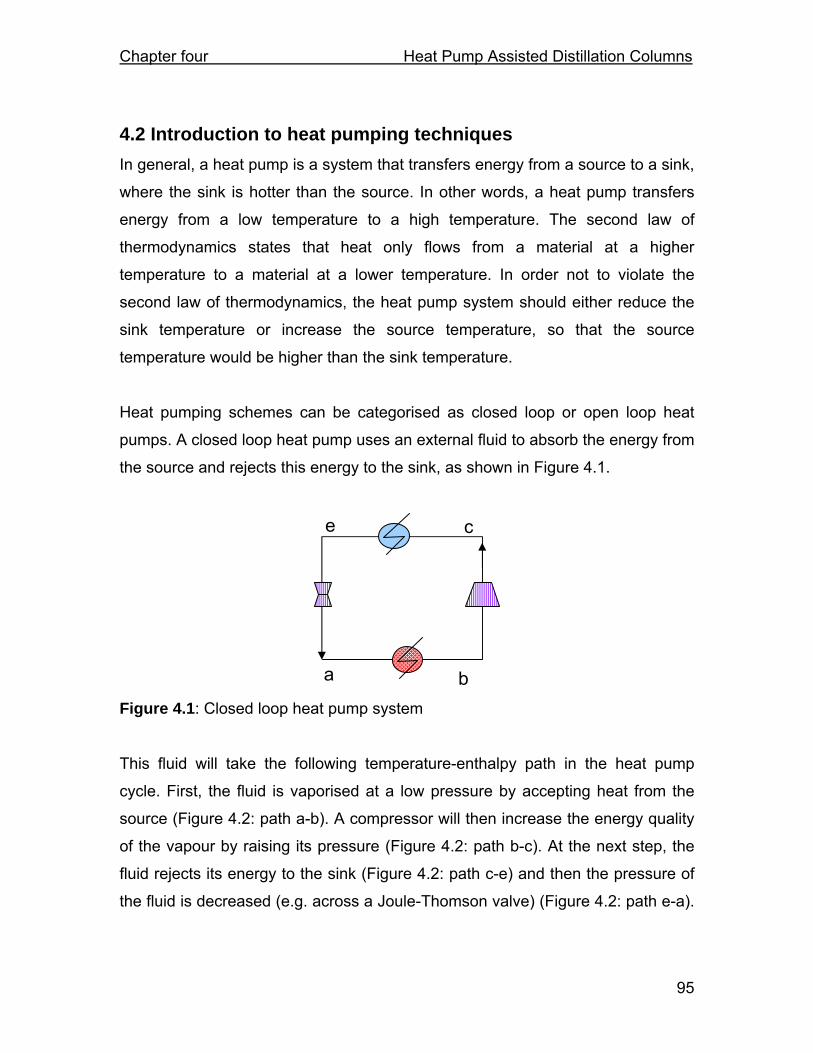
Chapter four Heat Pump Assisted Distillation Columns
95
4.2 Introduction to heat pumping techniques In general, a heat pump is a system that transfers energy from a source to a sink,
where the sink is hotter than the source. In other words, a heat pump transfers
energy from a low temperature to a high temperature. The second law of
thermodynamics states that heat only flows from a material at a higher
temperature to a material at a lower temperature. In order not to violate the
second law of thermodynamics, the heat pump system should either reduce the
sink temperature or increase the source temperature, so that the source
temperature would be higher than the sink temperature.
Heat pumping schemes can be categorised as closed loop or open loop heat
pumps. A closed loop heat pump uses an external fluid to absorb the energy from
the source and rejects this energy to the sink, as shown in Figure 4.1.
Figure 4.1: Closed loop heat pump system
This fluid will take the following temperature-enthalpy path in the heat pump
cycle. First, the fluid is vaporised at a low pressure by accepting heat from the
source (Figure 4.2: path a-b). A compressor will then increase the energy quality
of the vapour by raising its pressure (Figure 4.2: path b-c). At the next step, the
fluid rejects its energy to the sink (Figure 4.2: path c-e) and then the pressure of
the fluid is decreased (e.g. across a Joule-Thomson valve) (Figure 4.2: path e-a).
b
c e
a

Chapter four Heat Pump Assisted Distillation Columns
96
Afterwards, the fluid is recycled and re-vaporised by heat exchange against the
source.
Figure 4.2: Temperature-enthalpy diagram for a closed loop heat pump
An open loop heat pump, however, uses a process fluid as the cycle fluid. An
open loop heat pump scheme allows a process stream that needs cooling
(source) to exchange heat with a process stream that needs heating (sink), while
the source is colder than the sink. Therefore, without interference, this heat
transfer is not feasible. To overcome the infeasibility, the open loop heat pump
system has two options: increasing the pressure and hence the temperature of
the source; or reducing the pressure of the sink and hence its temperature.
Figure 4.3: Open loop heat system
Figure (4.3) shows an open loop heat pump which uses Option 1. At Point a, the
heat pump accepts a process fluid at vapour phase. The pressure of the process
a
b c
e d
f
Process stream
a b
c
e d
T
H
Process sink stream
Process source stream
Process stream

Chapter four Heat Pump Assisted Distillation Columns
97
fluid is raised in the compressor to Point b. The heat pump then uses another
process stream (which needs heating) to condense the vapour. The liquefied
process stream is let down in a throttle valve. As the result of throttling the liquid,
some vapour will be produced (Point e), which is recycled back to the
compressor. The liquefied process stream at the required pressure is returned to
the process.
Using the heat pump scheme may decrease operating costs when a large
amount of heat can be transferred with little work (compared with the operating
cost of providing utility for the reboiler and condenser in the distillation column).
Depending on the relative cost of utilities (for the reboiler and condenser) to the
cost of the energy for driving the compressor (e.g. cost of electricity), heat
pumping may be a cheaper option in terms of operating cost.
By employing a vapour recompression scheme, the constraint on the pressure of
the distillation column to use the cheaper and available external utility can be
relaxed. Usually the pressure of a distillation column is chosen so that cooling
water and cheaper steam can be used in the condenser and the reboiler.
However, if the distillation column is heat pumped, then the pressure can be
selected for an efficient separation. By operating at a more efficient pressure, the
reflux requirement and therefore the heat duties can also be reduced. Moderate
column pressure is also advantageous for the structural design of the column.
A compressor is an essential piece of equipment in a heat pump scheme. The
compressor and its drivers are expensive, both in terms of capital and operating
costs and this is a drawback for the heat pumped systems.
Overall, switching to vapour recompression scheme may result in reduction in the
energy costs at the expense of greater capital cost, and mechanical complexity.
In the next section, an open loop heat pump is compared with a closed loop
system when they are applied to a distillation problem.

Chapter four Heat Pump Assisted Distillation Columns
98
4.3 Comparison between open loop and closed loop heat pumps in a distillation column Figure 4.4 shows a distillation column such that its reboiler and condenser are
integrated with a closed loop heat pump. Figure 4.5 shows a distillation column
integrated using an open loop heat pump.
Figure 4.4: Distillation column Figure 4.5: Distillation column integrated by a closed loop heat pump integrated by an open loop heat pump
Installing an open loop heat pump, instead of integrating the reboiler and
condenser through a closed loop heat pump, can introduce benefits to the
process in some cases. Open loop heat pumps condense the top vapour of the
column and reboil the bottom liquid in a single heat exchanger, as shown in
Figure 4.5. This heat exchanger, known as the reboiler-condenser, satisfies the
demands of two process streams simultaneously. However, integration, by
applying closed loop heat pump technique, requires at least two heat
exchangers, as shown in Figure 4.4. In each of these exchangers, a minimum
temperature approach between the process fluid and the cycle working fluid is
required. The temperature-enthalpy diagram in Figure 4.6 illustrates this point.
The temperature difference between the source and the sink between which the
heat pump operates plus the minimum temperature approaches in the heat pump
evaporator and condenser is called the temperature lift. Therefore, the
Closed loop heat pump
Open loop heat pump Reboiler-condenser

Chapter four Heat Pump Assisted Distillation Columns
99
temperature lift for an open loop heat pump will be smaller (by a minimum
temperature approach, as shown in Figure 4.7), compared to the temperature lift
for a closed loop heat pump, both operating between the same heat source and
heat sink temperatures. This can result in lower shaft power consumption in the
open loop heat pump cycle, as the shaftwork required is also a function of
temperature lift.
Figure 4.6: Temperature-enthalpy Figure 4.7: Temperature-enthalpy diagram for a closed loop heat pump diagram for an open loop heat pump
Another benefit of an open loop heat pump over a closed loop heat pump is the
elimination or reduction of the required external cycle fluid. This both introduces
savings related to the reduction of the utility material and reduces the complexity
of the process compared to the closed loop heat pump option.
In the remaining parts of this chapter, open loop heat pumps in the distillation
column are discussed. Closed loop heat pumps are discussed in detail in
Chapter 6.
4.4 Various configurations and structures of open loop heat pumps As discussed previously, an open loop heat pump uses a process fluid as the
cycle fluid. Also, there are two strategies for open loop heat pumping:
T
H
Process fluid
Cycle fluid
2 minimum temperature approaches
T
H
Process fluid (e.g. column bottom liquid)
A single minimum temperature
approach
Process fluid (e.g. column
overhead vapour)

Chapter four Heat Pump Assisted Distillation Columns
100
compressing the source stream and expanding the sink stream. In the context of
applying open loop heat pump to a stand alone distillation column (as against a
distillation column in a sequence), these two options translate into two schemes:
mechanical vapour recompression, as illustrated in Figure 4.5 and bottom liquid
flash, as shown in Figure 4.8.
Figure 4.8: Bottom liquid flash heat pumped column
In a distillation column, the overhead vapour feed to the condenser is a source
stream and the bottom liquid feed to the reboiler is a sink stream. Obviously, the
direct heat transfer from the condenser to the reboiler is infeasible, since the
condenser is colder than the reboiler. If the vapour recompression scheme is
applied on a single distillation column, the vapour leaving the top of the column is
compressed to raise its temperature, as shown in Figure 4.5. The temperature of
the high pressure overhead vapour should be higher than the reboiler
temperature. The overhead vapour is then condensed to provide the reflux liquid.
This liquid is let down to the pressure of the column before returning to the
distillation column (Annakou and Mizsey, 1995).
If bottom flash is to be applied, the bottom liquid of the distillation column is
flashed across an expansion valve. Hence, its temperature is dropped to enable
the heat transfer between this stream and the overhead vapour of the distillation
column. After the bottom liquid is partly vaporised by the overhead vapour, the
generated vapour is compressed again to be sent back to the distillation column
as the stripping vapour, as illustrated in Figure 4.8 (Annakou and Mizsey, 1995).

Chapter four Heat Pump Assisted Distillation Columns
101
In practice, bottom liquid flash is seldom employed. This scheme carries a double
penalty, as a high pressure liquid with high quality energy is degraded in a Joule
Thomson valve without generating any type of energy. The degrading of the
bottom liquid is performed only to enable it to accept heat from a low-temperature
source. Another penalty occurs when, in order to send the bottom stream back to
the column, its pressure should be raised. So, an extra amount of compression
energy should be injected to the process. Obviously, this analysis suggests that
this scheme is not efficient. However, it should be mentioned that lowering the
pressure of process stream in order to produce refrigerated temperatures is
widely used in industry. The application of process stream expansion should be
justified in the overall process and this work considers employing this strategy for
providing the refrigerated utility in Chapter 6.
A mechanical vapour recompression (MVR) scheme may need auxiliary
condenser and reboiler heat exchangers to provide the necessary duties for the
column (Figure 4.9). The auxiliary equipment may be required for control and
flexibility purposes or for servicing the balance duty required by the distillation
column that is not provided in the reboiler-condenser heat exchanger (Meili and
Stuecheli, 1987; Sloley, 2001).
Figure 4.9: Examples of heat-pumped assisted distillation columns with auxiliary reboiler and/or condenser
Auxiliary
condenser Auxiliary
condenser
Auxiliary
reboiler
Auxiliary
reboiler

Chapter four Heat Pump Assisted Distillation Columns
102
4.5 Interactions between column operating parameters and open loop heat pump systems Using the heat pump scheme in a column with high energy demand can be
economic. The energy exchange requirement of the column and the economic
advantages of the heat pump system can be influenced by several parameters,
such as column pressure, reflux ratio, feed rate, number of plates, pressure loss
of the column and column internals. In addition, the relative cost of energy
required in heat pump and utility in the distillation column is another important
factor, influencing the economics of the heat pump application.
The following sections will analyse the interactions between the mechanical
vapour recompression scheme and column design parameters. However,
beforehand a discussion is presented on parameters that can be used to
determine the performance of a heat pump system. These parameters will be
used as tools for further analysis of the interactions between distillation and heat
pump system.
4.5.1 Parameters affecting the performance of a heat pump system The key intention in this section is to determine the parameters affecting the
performance of a heat pump, which can also be related to the distillation column
operating parameters. A useful tool towards showing the performance of a heat
pump system is the coefficient of performance. The coefficient of performance
(COP) is defined as the heat load absorbed or rejected (Q) by the heat pump
divided by the shaftwork (W) required for the heat pump operation.
WQCOP = 4.1
The higher the value of the COP, the more efficient the heat pump system. The
value of the shaftwork in the COP can indicate whether applying the heat pump

Chapter four Heat Pump Assisted Distillation Columns
103
system is economic or not. The power requirement of the heat pump in a
distillation column is a function of the heat load on the cycle.
COPQW = 4.2
Installing a heat pump on a distillation column saves both external hot and cold
utility. However, usually either the utility required in the reboiler or the utility
required in the condenser dominates the operating costs. Therefore, reducing the
load of the more expensive utility will become the objective of the heat pump
installation. Hence, the heat load value of this (more expensive) utility will appear
in the calculation of the coefficient of performance. Therefore:
WQCOP C
cooling = 4.3
where Qc is the absorbed heat by heat pump.
WQCOP h
heating = 4.4
where Qh is the rejected heat by heat pump. Moreover, for a heat pump at
maximum theoretical efficiency (i.e. Carnot efficiency), it can be shown that (Elliot
and Lira, 1999):
c
c
h
h
TQ
TQ
= 4.5
where Tc and Th are the temperature of the cold and hot reservoirs (respectively)
between which the heat pump cycle operates. Substituting Qc from Equation 4.5

Chapter four Heat Pump Assisted Distillation Columns
104
into the overall energy balance around the heat pump system (i.e.:
chideal QQW −= ) gives:
c
chc
ideal
TTTQW −
⋅= 4.6
Substituting Qh from Equation 4.5 into the overall energy balance around the heat
pump system gives:
h
chh
ideal
TTTQW −
⋅= 4.7
As Equations 4.6 and 4.7 illustrate, the work demand in the heat pump system
depends directly on the temperature difference between the hot and cold
reservoir (between which heat pump operates). This temperature difference is
called the temperature lift. The smaller the temperature lift is, the lower the heat
pump compressor power consumption will be.
Equations 4.6 and 4.7 evaluate the ideal power demand in the heat pump cycle.
An efficiency factor, η , can be used for these equations to estimate the actual
power demand. This efficiency has a typical value of 0.4 to 0.6 (Smith, 2005). For
instance:
c
chc
c
chc
actual
TTT6.0Q
TTTQW eApproximat −
⋅⋅=−
⋅⋅= η 4.8
However, the actualW calculated by Equation 4.8 is still an approximation of the
actual power required in the heat pump cycle. This equation is not taking into
account the effect of the type of cycle fluid, which is also another factor affecting
the performance in the heat pump system (Shelton and Grossmann, 1985).

Chapter four Heat Pump Assisted Distillation Columns
105
The temperature lift and the load on the heat pump affect the power demand of
the heat pump system. These two parameters can be related to the operating
parameters of the distillation column. In the following section, these two
parameters are used for studying the relation between the performance of the
heat pump and the column operating parameters in a heat-pump assisted
distillation column.
4.5.2 How may the operating parameters of the distillation column affect the heat pump performance?
4.5.2.1 Reflux ratio
Reflux ratio is a key variable in the performance of a distillation column. Figure
4.10 shows the part of the column above the feed, the rectifying section. L is the
molar flowrate of the liquid which is recycled back to the distillation column. D is
the molar flowrate of the distillate. The reflux ratio, RR, is defined to be:
DLRR = 4.9
In the McCabe Thiele design method for distillation columns, the operating line in
the rectifying section is a function of the reflux ratio (Smith 2005):
D,in,i1n,i x1RR
1x1RR
RRy+
++
=+ 4.10
where, n,in,i x and y are the compositions of component i in the vapour and liquid
phase at stage n, respectively. For a given separation, increasing the reflux ratio
will increase the gradient of the rectifying operating line, moving it away from the
equilibrium line (Figure 4.10), therefore, decreasing the number of stages
required to achieve the separation. Alternatively, for a fixed number of stages (i.e.
an existing column) adjusting the reflux ratio will control the purity of the product,
the higher the reflux ratio the higher the purity of the distillate.
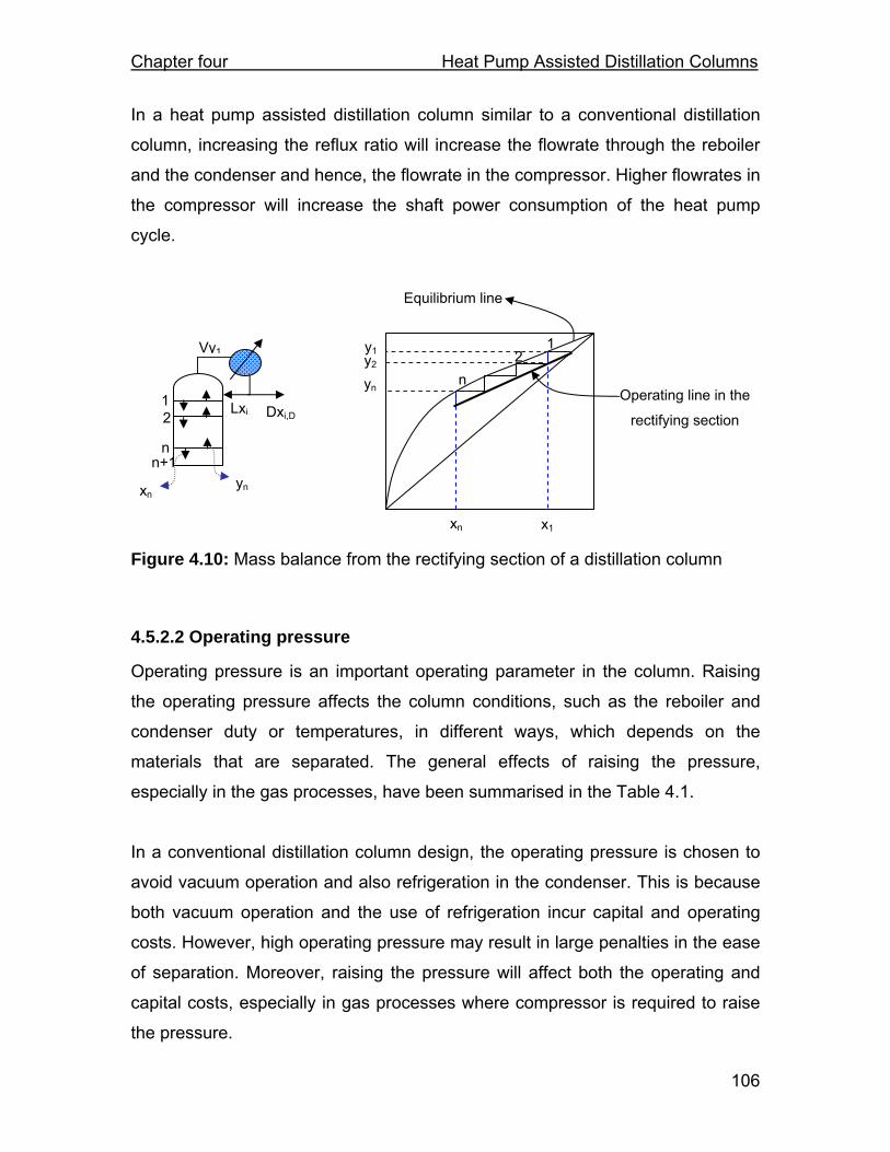
Chapter four Heat Pump Assisted Distillation Columns
106
In a heat pump assisted distillation column similar to a conventional distillation
column, increasing the reflux ratio will increase the flowrate through the reboiler
and the condenser and hence, the flowrate in the compressor. Higher flowrates in
the compressor will increase the shaft power consumption of the heat pump
cycle.
Figure 4.10: Mass balance from the rectifying section of a distillation column
4.5.2.2 Operating pressure
Operating pressure is an important operating parameter in the column. Raising
the operating pressure affects the column conditions, such as the reboiler and
condenser duty or temperatures, in different ways, which depends on the
materials that are separated. The general effects of raising the pressure,
especially in the gas processes, have been summarised in the Table 4.1.
In a conventional distillation column design, the operating pressure is chosen to
avoid vacuum operation and also refrigeration in the condenser. This is because
both vacuum operation and the use of refrigeration incur capital and operating
costs. However, high operating pressure may result in large penalties in the ease
of separation. Moreover, raising the pressure will affect both the operating and
capital costs, especially in gas processes where compressor is required to raise
the pressure.
Lxi, Dxi,D
Vy1
12
n+1n
xn yn
1
n2
x1xn
y1
yn Operating line in the
rectifying section
Equilibrium line
y2
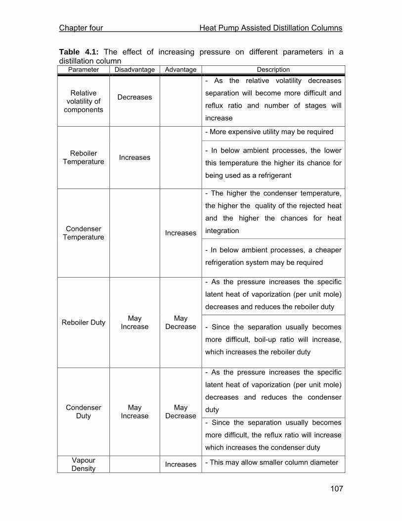
Chapter four Heat Pump Assisted Distillation Columns
107
Table 4.1: The effect of increasing pressure on different parameters in a distillation column
Parameter Disadvantage Advantage Description
Relative volatility of
components
Decreases
- As the relative volatility decreases
separation will become more difficult and
reflux ratio and number of stages will
increase
- More expensive utility may be required
Reboiler Temperature Increases
- In below ambient processes, the lower
this temperature the higher its chance for
being used as a refrigerant
- The higher the condenser temperature,
the higher the quality of the rejected heat
and the higher the chances for heat
integration Condenser Temperature Increases
- In below ambient processes, a cheaper
refrigeration system may be required
- As the pressure increases the specific
latent heat of vaporization (per unit mole)
decreases and reduces the reboiler duty
Reboiler Duty May Increase
May Decrease - Since the separation usually becomes
more difficult, boil-up ratio will increase,
which increases the reboiler duty
- As the pressure increases the specific
latent heat of vaporization (per unit mole)
decreases and reduces the condenser
duty Condenser Duty
May Increase
May Decrease
- Since the separation usually becomes
more difficult, the reflux ratio will increase
which increases the condenser duty
Vapour Density Increases - This may allow smaller column diameter
Chapter four Heat Pump Assisted Distillation Columns
108
Employing a heat pump assisted distillation column scheme can relax the
constraint on the column operating pressure. These constraints can be imposed
to use the available utility or to avoid expensive utility (such as refrigeration).
Consequently, the pressure may be optimised for an efficient separation and the
required reflux ratio and the number of stages can be reduced. The smaller the
number of stages in the column, the lower the pressure drop in the column.
Consequently, the temperature difference between the top and the bottom of the
column will be smaller. The decrease in the reflux ratio and the temperature
range in the column help in lowering the power demand in the heat pump. So,
these are positive consequences both for the column and the heat pump system.
In cases, where even at high pressures, refrigeration is required in the
condenser, integrating the condenser and the reboiler of the column through a
heat pump may be advantageous. The heat pump assisted system may use less
shaft power compared to the power required by the external refrigeration cycle.
Also, as mentioned above, the system may be allowed to operate in lower
operating pressures at the presence of open loop heat pump. The economic
benefit will be higher when the temperature difference between the reboiler and
the condenser is low, since less power will be required in the compressor.
4.5.2.3 Feed quality
Feed quality is another variable that influences the performance of a distillation
column. The feed quality, q, is the ratio of the heat required to vaporise 1 mole of
feed to the molar latent heat of vaporisation of feed. For a saturated liquid feed, q
equals 1 and for a saturated vapour feed, q equals 0. Heating the feed most often
(Smith, 2005):
• increases the number of trays in the rectifying section but decreases trays
in the stripping section;
• requires less heat in the reboiler but more cooling in the condenser.
Chapter four Heat Pump Assisted Distillation Columns
109
Cooling the feed most often reverses these effects. Whether these effects are
good or bad for the operating and capital costs of the overall separation
sequence depends on the relative costs of hot and cold utility required at each
level and the operating and capital cost tradeoffs.
Feed quality will affect the value of heat load in the reboiler and condenser and
consequently affects the heat pump performance. Moreover, heating or cooling
the feed results in having a heat source or sink at an intermediate temperature
between that of the reboiler and condenser. If heat pumping is allowed between
different sources and sinks in the process (instead of only between the reboiler
and condenser of the same column), this heater or cooler becomes an attractive
option for heat pumping. This is because the heat pump system has lower power
demand for smaller temperature lifts.
4.6 Design and optimisation of heat pump assisted distillation column 4.6.1 Introduction So far in this chapter, open loop heat pump systems have been introduced. The
objective is to develop a systematic methodology for simulation and optimisation
of heat pump assisted distillation column. A shortcut design technique is desired
to avoid the computational complexities in optimisation. Also, as it is intended to
compare the performance of heat pump assisted distillation column with other
types of distillation devices and heat integration options (especially in terms of
energy consumption), consistent shortcut models for all devices are required.
This section addresses the design principles and procedures of the open loop
heat pump system. The manner in which the heat pump system and the
distillation column are coupled is also described.
In a distillation column with a mechanical vapour recompression (MVR) scheme,
the overhead vapour passes through the MVR compressor. The overhead vapour
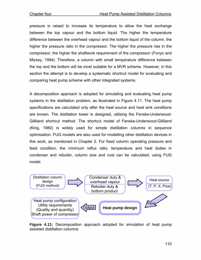
Chapter four Heat Pump Assisted Distillation Columns
110
pressure is raised to increase its temperature to allow the heat exchange
between the top vapour and the bottom liquid. The higher the temperature
difference between the overhead vapour and the bottom liquid of the column, the
higher the pressure ratio in the compressor. The higher the pressure rise in the
compressor, the higher the shaftwork requirement of the compressor (Fonyo and
Mizsey, 1994). Therefore, a column with small temperature difference between
the top and the bottom will be most suitable for a MVR scheme. However, in this
section the attempt is to develop a systematic shortcut model for evaluating and
comparing heat pump scheme with other integrated systems.
A decomposition approach is adopted for simulating and evaluating heat pump
systems in the distillation problem, as illustrated in Figure 4.11. The heat pump
specifications are calculated only after the heat source and heat sink conditions
are known. The distillation tower is designed, utilising the Fenske-Underwood-
Gilliland shortcut method. The shortcut model of Fenske-Underwood-Gilliland
(King, 1980) is widely used for simple distillation columns in sequence
optimisation. FUG models are also used for modelling other distillation devices in
this work, as mentioned in Chapter 2. For fixed column operating pressure and
feed condition, the minimum reflux ratio, temperature and heat duties in
condenser and reboiler, column size and cost can be calculated, using FUG
model.
Figure 4.11: Decomposition approach adopted for simulation of heat pump assisted distillation columns
Heat source
(T, P, X, Flow)
Heat pump design
Heat pump configuration Utility requirements
(Quality and quantity) Shaft power of compressor
Distillation column design
(FUG method) Reboiler duty & bottom product
Condenser duty & overhead vapour
Input Output

Chapter four Heat Pump Assisted Distillation Columns
111
The specifications of the condenser and reboiler streams (i.e. temperature,
pressure, compositions, and flow rates) and the required phase changes are
produced for the heat pump design algorithm. Thereafter, the heat pump
algorithm will determine the following information:
• heat pump configuration;
• utility requirement (quantity and quality);
• shaft power of compressor.
4.6.2 Heat pump design procedure In this work, while optimising the separation sequence problem, the optimisation
framework may determine that a specific simple separation task should be
carried out in a simple heat pump assisted distillation column. The simple
distillation column is then designed using FUG method and the reboiler and the
condenser streams are sent as the heat source and the heat sink to the heat
pump design algorithm. A total condenser is assumed for the distillation column
in the present model. The model for partial condenser can be implemented in the
future.
The heat pump design algorithm will first check the feasibility of the heat pumping
between the proposed candidates. The critical properties of the overhead vapour
limit the amount of its pressure rise. In order to avoid the critical region of the
overhead vapour, the process is constrained in raising the overhead stream
pressure. This pressure, when raised, should be away from its critical pressure.
Avoiding the critical pressure is required because the condensation of the vapour
is not possible above the critical pressure. Therefore, the design algorithm
ensures that the operating conditions are sufficiently far from critical conditions.
)X(TT topcriticalbubble
vapourtop < 4.11

Chapter four Heat Pump Assisted Distillation Columns
112
bubblevapourtopT is the bubble temperature of the column top vapour after compression
in the compressor of the heat pump. )X(T topcritical is the critical temperature for
the mixture leaving the top of column. In this work as a rule of thumb, the
following constraint is enforced:
10)X(TT topcriticalbubble
vapourtop −< 4.12
If the required temperature for the overhead stream demands pressures higher
than )X(T topcritical , the heat pump scheme is not feasible.
If the system fulfils the critical condition constraint, then the algorithm checks if
the distillation column is operating at above ambient or below ambient conditions.
required. design ambient boveaDTTT If
required. design ambient belowDTTT If
ambtop
ambtop
→+>
→+<
Depending on the result, the appropriate design procedure is selected as follows:
4.6.2.1 Below-ambient design procedure
The structure for a heat pump assisted distillation column in a below ambient
process is shown in Figure (4.12).

Chapter four Heat Pump Assisted Distillation Columns
113
Figure 4.12: The structure for heat pump assisted distillation column in a below ambient process
In the scheme shown in Figure (4.12), the majority or all of the heating demand of
the distillation column is satisfied in the reboiler-condenser (Ereb,cond) by cooling
and liquefying the column overhead vapour. In order to increase the temperature
of the overhead vapour (Vtop) to allow the heat transfer with the bottom liquid
(Bbot), the pressure of the vapour is raised in the compressor. Energy in the form
of work, Winput, is added to the vapour (Vtop) to increase its temperature.
)P,T,X(HW)P,T,X(H compmt
compmtmt
compmtinputmtmtmtmt =+ 4.13
where, mtH is the enthalpy of the overhead stream before entering the
compressor and compmtH is the enthalpy of the overhead stream after leaving the
compressor. compmtP is chosen so that:
DT)P,X(T)P,X(T colbot
dewbot
compmtmt
bub,compmt += 4.14
That is the pressure ratio in the compressor is determined so that the bubble
temperature of the overhead vapour, )P,X(T compmtmt
bub,compmt , equals the dew
F
D
B
Vtop, Xtop, Pcol, Ttop
Vmt, Xmt, Pcol, Tmt
Vmtcomp, Xmt, Pmt
comp,
Tmtcomp
Ereb,cond
Vmtcomp,
Xmtcomp,
Pmtcomp,
Tmtcomp, bubble
Bbot, Xbot, Pcol, Tbot
Pcol
Xmtexp, Pcol, Tmt
exp
Flashed vapour from
the heat pump system
FV, Y
∆Q
∆Q

Chapter four Heat Pump Assisted Distillation Columns
114
temperature of the bottom liquid, )P,X(T colbot
dewbot , plus the minimum approach
temperature, DT .
Overall energy balance around the system is given by:
0QWHHH inputbdf =−+−− Δ 4.15
If ∆Q is positive, an auxiliary condenser is required in the process. Otherwise, a
trim reboiler should be coupled with the reboiler-condenser to meet the energy
balance of the system.
∆Q > 0 Auxiliary condenser is required.
∆Q < 0 Auxiliary reboiler is required.
When the energy balances around the system determine that a trim reboiler is
required, the bottom liquid from the distillation column is divided into two parts.
One part is sent to the reboiler-condenser to exchange heat with the condenser
stream. The second part is vaporised using an external utility to provide the
column with the required vapour flow.
The main difference between a below ambient and above ambient heat pump
design is the location of the trim condenser. In a below ambient process, cooling
of some streams requires temperatures below the temperature provided by the
ambient utility. Therefore, either chilled water or a refrigeration system is utilised
for satisfying the requirements of these streams. A refrigeration process is
inherently expensive. As a result, there is an incentive to avoid cryogenic (sub-
ambient) temperatures. Hence, if a trim condenser is required in a sub-ambient
distillation column, it is located after the compressor. This arrangement increases
the condensing temperature (bubble temperature) of the vapour and may
eliminate or reduce the need for refrigerated utility in the condenser. Certainly, if
still refrigerated utility is needed, this utility is required at higher temperatures.

Chapter four Heat Pump Assisted Distillation Columns
115
Providing refrigerated utility at the higher temperatures will be cheaper and
requires less shaftwork. Overall, it is more economic to place the trim condenser
after the compressor in a sub-ambient distillation column.
The energy balance in the reboiler condenser will give:
[ ][ ] latentbotbot
compmt
latentmt
compmt
dewmt
compmt
compmtmtmt HB)p(h)p(TT)p(CpV ×=+−×× 4.16
Figure 4.13: Heat pump assisted distillation column with an auxiliary condenser in a below ambient process
A compressed and condensed overhead stream of the distillation column is
expanded to the column pressure, colP , through a throttle valve in an isenthalpic
process.
)P,T,X(H)P,T,X(H colexpmtmt
expmt
compmt
compmtmt
compmt = 4.17
Through the expansion process, part of the liquefied overhead vapour is
vaporised. The vapour fraction, VapFrac , is given by:
)P,X(H)P,Y(H)P,X(HH
VapFrac coltop
bubblemt
coldewmt
coltop
bubblemt
compmt
−−
= 4.18
where, Y is the composition of the vapour in equilibrium with the available liquid
after expansion, Xtop. The produced liquid and vapour are separated in a flash
drum. The resulting vapour is then recycled back to the heat pump cycle. The
Auxiliary
condenser
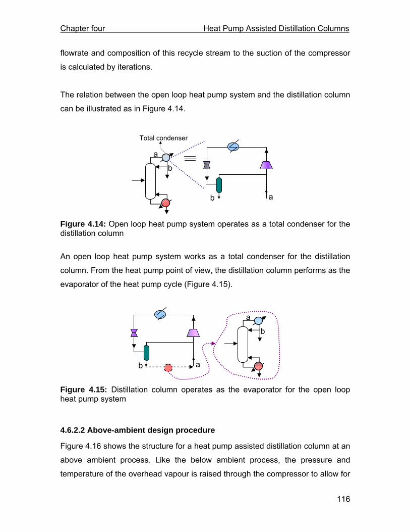
Chapter four Heat Pump Assisted Distillation Columns
116
flowrate and composition of this recycle stream to the suction of the compressor
is calculated by iterations.
The relation between the open loop heat pump system and the distillation column
can be illustrated as in Figure 4.14.
Figure 4.14: Open loop heat pump system operates as a total condenser for the distillation column
An open loop heat pump system works as a total condenser for the distillation
column. From the heat pump point of view, the distillation column performs as the
evaporator of the heat pump cycle (Figure 4.15).
Figure 4.15: Distillation column operates as the evaporator for the open loop heat pump system
4.6.2.2 Above-ambient design procedure
Figure 4.16 shows the structure for a heat pump assisted distillation column at an
above ambient process. Like the below ambient process, the pressure and
temperature of the overhead vapour is raised through the compressor to allow for
a
b
ab
Total condenser
a
b
ab
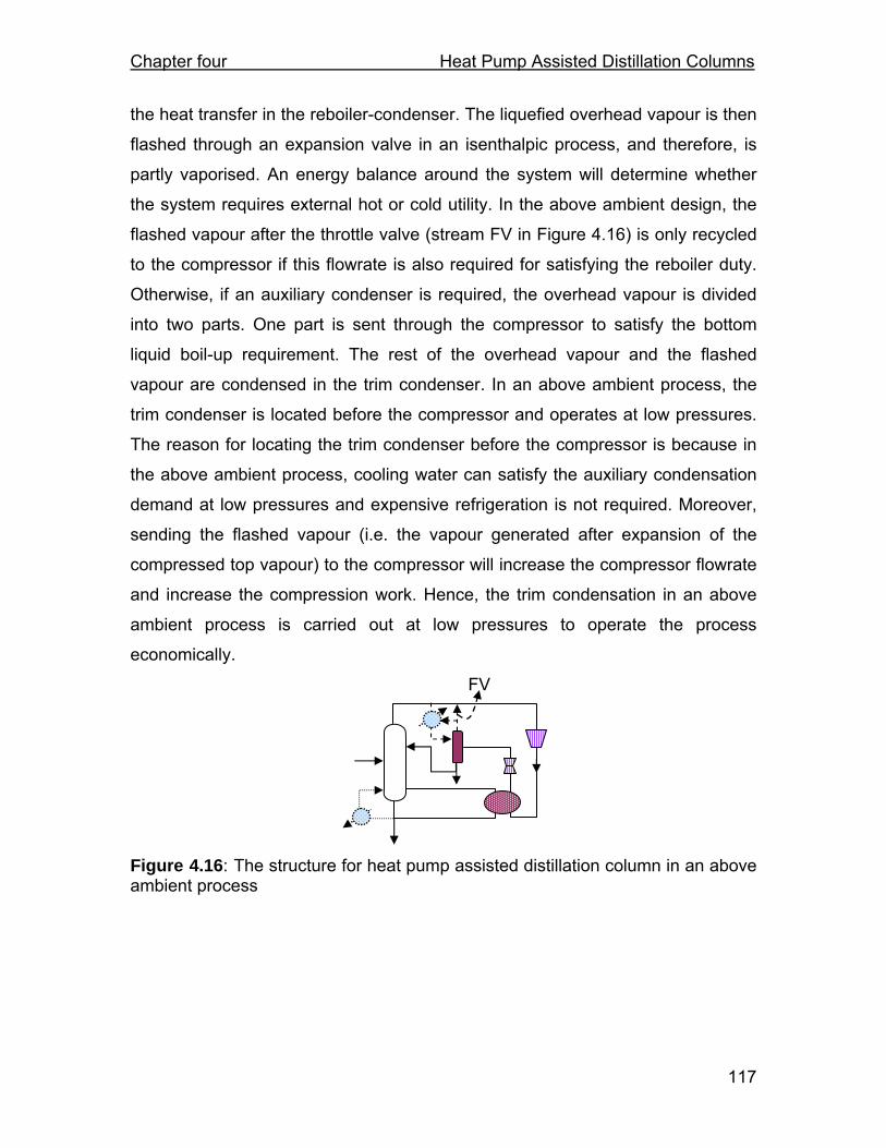
Chapter four Heat Pump Assisted Distillation Columns
117
the heat transfer in the reboiler-condenser. The liquefied overhead vapour is then
flashed through an expansion valve in an isenthalpic process, and therefore, is
partly vaporised. An energy balance around the system will determine whether
the system requires external hot or cold utility. In the above ambient design, the
flashed vapour after the throttle valve (stream FV in Figure 4.16) is only recycled
to the compressor if this flowrate is also required for satisfying the reboiler duty.
Otherwise, if an auxiliary condenser is required, the overhead vapour is divided
into two parts. One part is sent through the compressor to satisfy the bottom
liquid boil-up requirement. The rest of the overhead vapour and the flashed
vapour are condensed in the trim condenser. In an above ambient process, the
trim condenser is located before the compressor and operates at low pressures.
The reason for locating the trim condenser before the compressor is because in
the above ambient process, cooling water can satisfy the auxiliary condensation
demand at low pressures and expensive refrigeration is not required. Moreover,
sending the flashed vapour (i.e. the vapour generated after expansion of the
compressed top vapour) to the compressor will increase the compressor flowrate
and increase the compression work. Hence, the trim condensation in an above
ambient process is carried out at low pressures to operate the process
economically.
Figure 4.16: The structure for heat pump assisted distillation column in an above ambient process
FV
Chapter four Heat Pump Assisted Distillation Columns
118
4.7 Comparing heat pump option with direct heat integration options In this text, two heat integrated exchangers are considered to be directly heat
integrated, when the heat sources and the heat sinks exchange heat without
using any auxiliary streams or sources of energy, e.g. process stream to process
stream. On the other hand, when energy is transferred from one stream to
another via an intermediate system or material, it is called indirect heat
integration. Examples of this include transfer of heat by generating steam or
using heat pump.
Bearing in mind the proposed classification, direct heat integration seems to be
the most simple and economic way of energy saving. However, direct heat
integration is sometimes faced by process or mechanical constraints. For
instance, to directly integrate a source with a sink in a separation sequence, the
associated devices should operate at different operating pressures. This may
result in a more expensive utility for the reboiler of the column at higher pressure
and offset the savings introduced by direct heat integration. Another scenario
may be that the required pressure cannot be implemented in practice because of:
material constraints, mechanical constraints (especially in retrofit cases) or
process constraints (e.g.: poor separation efficiency, product decomposition).
In the case of stand-alone distillation units, or when there are restrictions on the
integration of the distillation columns, a heat pump assisted distillation column is
the most promising energy saving technique.
Another advantage of heat pumped distillation system is that it offers integration
opportunities without interfering with the operating conditions in the column.
Therefore, the operating conditions of the system can be optimised
independently, considering only the enhancement of the separation process.
Chapter four Heat Pump Assisted Distillation Columns
119
Like other energy integration methods, heat pumps reduce the primary energy
consumption and therefore, lead to a more efficient, economic and
environmentally friendly process.
A robust methodology should maintain the ability to compare different integration
opportunities with one another simultaneously and to choose the optimum design
for the specific problem in hand.
4.8 Illustrative example In this section a short study is presented to illustrate the application of the
developed model for heat pump assisted distillation column in this work. In
petrochemicals, high purity propylene is required to meet polymer-grade specifications for propylene in the petrochemical industry. Therefore, propylene should
be purified from other hydrocarbons and propane. The propylene/propane separation is
a difficult separation, historically requiring two columns to accommodate the high reflux
and large number of distillation trays. This separation is a potential candidate for
applying heat pump system due to the close boiling point of propane and propylene and
is used in the present case study.
The components of a mixture with the mole fraction of 0.92 and 0.08 for propylene and
propane; respectively, are to be separated to produce a propylene product with a
concentration of 99.6%. The application of heat pump assisted distillation column will be
compared with the conventional distillation column. Direct heat integration opportunities
are also exploited. The operating pressure range of 1 bar to 10 bar is explored. Different
feed quality values are examined. The products are required at 2 bar and saturated
liquid conditions. The optimisation tool employed in this study (enhanced simulated
annealing) and the methodology for evaluating the cost of the refrigerated utility (that
may be required) in this case study is presented in Chapter 5 and 6. The intention in this
section is to illustrate the heat pump model. The total cost of the C3 splitter is studied.
The best option for the above study is shown in Figure 4.17. A heat pump assisted
distillation column is chosen over the other available options of heat integrated
distillation column. The column is operating at 4.5 bar with a feed quality of 0.7. The

Chapter four Heat Pump Assisted Distillation Columns
120
temperatures in the column at the condenser and reboiler points are -7.5 ˚C and -2.2 ˚C.
The small temperature difference between the reboiler and condenser points in the
column creates a good opportunity for employing heat pump assisted distillation column.
The required pressure ratio is 1.3 and the compressor energy demand in this design is
7.9 MJ per kmol of the feed to the column. The scheme in Figure 4.17 shows that this
design needs a small trim condenser. Since the column is operating at below ambient
temperature, the condenser is located after the compressor so that part of the cooling
would be required at higher temperature. No auxiliary reboiler is required as the
condensation of the overhead vapour of the column provides the heating required for the
reboiler of the column.
Figure 4.17: Heat pump assisted distillation column scheme for propylene / propane separation
This example applies the heat pump model in a below-ambient process. In the
next chapter, the application of the heat pump model in an above ambient case
study will also be presented.
4.9 Summary This chapter presents and analyses the concept of open loop heat pumping. A
shortcut model for simulation and evaluation of heat pump assisted distillation
columns is also presented. This model can be integrated with the synthesis
framework for heat integrated separation sequences (composed of the
methodologies presented in Chapter 2 and 3) and allows the comparison of heat
pump assisted distillation column with other available heat integration techniques
in the framework. The next chapter will elaborate on the optimisation framework
of heat integrated separation sequence synthesis.
Auxiliary condenser
Reboiler-condenser

Chapter four Heat Pump Assisted Distillation Columns
121
4.10 Nomenclature B Column bottom product stream
botB Molar column bottom flowrate (kmol/s) in the reboiler-condenser
COP Coefficient of performance
Cp Specific heat capacity of the stream (kJ/kmol ˚C)
D Top product flowrate of distillation column (kmol/s)
DT Minimum approach temperature
Ereb,cond Reboiler-condenser heat exchanger
F Column feed stream
FV Flashed vapour from the heat pump system
H Enthalpy latenth Latent heat of stream (kJ/kmol)
L Reflux flowrate (kmol/s)
Pcol Column pressure
Q Heat load (kW, MW)
CQ Absorbed heat by the heat pump
hQ Rejected heat by the heat pump
∆Q The duty of the auxiliary heat exchanger (either reboiler or condenser)
in a heat pump assisted distillation column
P Pressure
RR Reflux ratio
T Temperature
cT Temperature of cold reservoir from which heat is absorbed by the
heat pump
criticalT Critical temperature
hT Temperature of hot reservoir to which heat is rejected by the heat
pump
V Open loop heat pump stream
mtV Molar flowrate of the mixture of overhead stream and flashed vapour
from the heat pump system
Chapter four Heat Pump Assisted Distillation Columns
122
VapFrac Vapour fraction in the heat pump system flashed vapour
W Shaftwork (kW, MW)
actualW Actual amount of shaftwork required by a heat pump (kW, MW)
Wideal Ideal amount of shaftwork required by a heat pump (kW, MW)
inputW Input shaftwork to the heat pump system
x Mole fraction of component in liquid
X Molar composition
y Mole fraction of component in vapour
Y Mole fraction of the flashed vapour from the heat pump system
Sub- and super- scripts
amb Ambient condition
B Column bottom product
bot Condition at bottom of the distillation column
bubble Bubble point of the liquid mixture
cmp Compressed stream condition
D Column top product
dew Dew point of vapour mixture
exp Expanded stream
f Column feed
mt Mixture of column overhead vapour and the flashed vapour from the heat
pump system
N Tray number in a distillation column
top Condition at top of the distillation column
Greek letters
η Efficiency factor for approximating the actual power demand of a heat
when using Carnot factor
Chapter five Optimisation framework
123
5 Chapter Five Optimisation framework
5.1 Introduction In the previous chapters, methodologies for synthesis and design of different
parts of a heat integrated separation sequence were discussed. The method for
the synthesis of a separation sequence adopted in this work is presented in
Chapter 2 and a model for considering heat integration opportunities is proposed
in Chapter 3. At this point, an optimisation tool is required to employ the
proposed models in previous chapters for optimising the heat-integrated
separation sequence. The present chapter introduces the optimisation approach
used in this work and the way it is implemented and integrated with the process
simulation models. A case study is presented to demonstrate the performance of
the proposed approaches.
5.2 Simulated annealing: To solve nonlinear, non-convex optimisation problems, meta-heuristic algorithms
have been used since 1952 (Robbins and Monro, 1951). Meta-heuristics are high
level strategies for exploring problem search space by using different methods
(Blum and Roli, 2003). Generally, the meta-heuristic algorithms employed for
optimisation are derivative-free. Simulated annealing is one of the common meta-
heuristic algorithms that have been applied in chemical engineering. The first
algorithms of simulated annealing were introduced independently by Kirkpatrick
et al. (1983) and Černý 1985.
Simulated annealing (SA) is a stochastic optimisation method, as in different
stages of the SA algorithm, some decisions are made based on probabilities.

Chapter five Optimisation framework
124
Simulated annealing is a point-to-point† based search method. To generate a
new trial solution, one optimisation variable of the present candidate solution is
changed and one new solution is generated. Therefore, the optimiser moves
from one point to another in the search space.
The simulated annealing algorithm is designed to have higher chances of finding
the global optimum than deterministic methods. For example, when the
optimisation problem is a minimisation problem, the simulated annealing
algorithm definitely accepts all the moves that reduce the objective function. The
moves that decrease the objective function are called downhill moves, while the
moves‡ that increase the objective function are referred to as uphill moves. SA
allows uphill moves to be accepted according to some rules and probabilities.
Hence, simulated annealing has the capacity to escape from local optima.
For instance, in Figure 5.1 point ‘a’ in valley ‘A’ is a local minimum and point b in
valley B is the global minimum of the objective function F(x). If the optimiser is
searching in valley ‘A’ in Figure 5.1, simulated annealing may accept the moves
in the directions of the arrow β. Hence, the optimiser may exit valley A and
continues the search in valley B, increasing the chance to find the global
optimum at point b. This simple illustration demonstrates that the simulated
annealing algorithm has the capacity of escaping local optima.
Examining the convergence of simulated annealing to the global optimum of the
function, has been the subject of much research effort (e.g. Aarts and Van
Laarhoven, 1985; Hajek, 1988; Hajek and Sasaki, 1989). Discussing the details
† The heuristic based optimisation methods can be classified in two categories: point-to-point methods and population based methods. In point-to-point methods, at each instant of optimisation, a single present solution is used to produce the next single solution. In a population based method, a group or pool of solutions are employed to generate the next group of candidate solutions, in each instant of optimisation. An example of population based optimisation method is Genetic Algorithm. ‡ In the point-to-point methods, the process of changing the current solution to produce the new solution is referred to as move. In each move, one of the optimisation variables is altered.
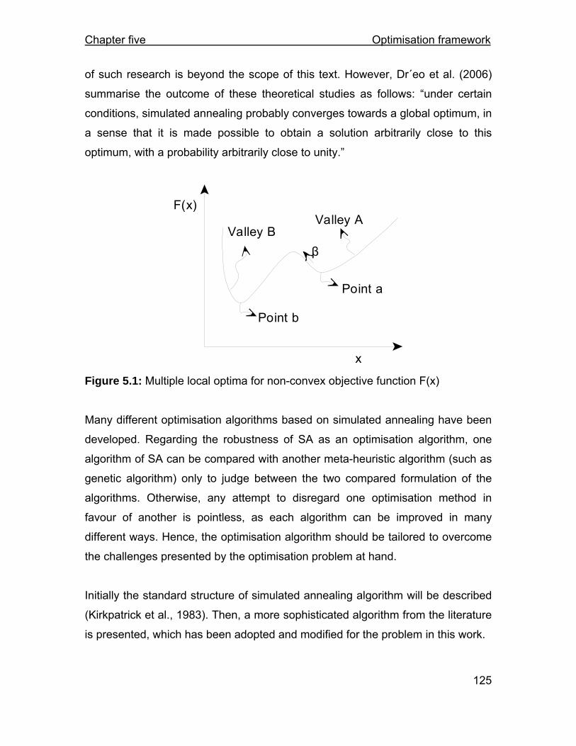
Chapter five Optimisation framework
125
of such research is beyond the scope of this text. However, Dr´eo et al. (2006)
summarise the outcome of these theoretical studies as follows: “under certain
conditions, simulated annealing probably converges towards a global optimum, in
a sense that it is made possible to obtain a solution arbitrarily close to this
optimum, with a probability arbitrarily close to unity.”
Valley B
Point b
Valley A
Point a
F(x)
x
β
Figure 5.1: Multiple local optima for non-convex objective function F(x)
Many different optimisation algorithms based on simulated annealing have been
developed. Regarding the robustness of SA as an optimisation algorithm, one
algorithm of SA can be compared with another meta-heuristic algorithm (such as
genetic algorithm) only to judge between the two compared formulation of the
algorithms. Otherwise, any attempt to disregard one optimisation method in
favour of another is pointless, as each algorithm can be improved in many
different ways. Hence, the optimisation algorithm should be tailored to overcome
the challenges presented by the optimisation problem at hand.
Initially the standard structure of simulated annealing algorithm will be described
(Kirkpatrick et al., 1983). Then, a more sophisticated algorithm from the literature
is presented, which has been adopted and modified for the problem in this work.

Chapter five Optimisation framework
126
5.3 ‘Standard’ simulated annealing algorithm 5.3.1 Origins of Simulated Annealing Kirkpatrick et al. (1983) were experts in statistical physics and interested in the
low energy configurations of disordered magnetic materials. They wanted to
numerically determine the variables associated with the low energy states of the
materials. Therefore, it was necessary to minimise the energy function in
disordered magnetic materials to find the values of the associated variables. The
energy function of such materials, however, presents several valleys of unequal
depths and finding the deepest valley (i.e. the global minimum) will not be
straightforward.
Kirkpatrick et al. (1983) (and independently Cerny (1985)) decided to take a
pattern from a practical technique used by metallurgists called annealing.
Through annealing, metallurgists obtain a “well ordered” solid state of minimal
energy for a material. Annealing consists of heating the material to a high
temperature and then lowering the temperature slowly, in order to avoid the
meta-stable structures, as shown in Figure 5.2-(a). The meta-stable structures
correspond with local minima of energy. The temperature shows the amount of
the energy of the material. If the temperature is reduced too fast, as in Figure
5.2-(b) (in other words, if the energy of the material is reduced too quickly), the
procedure is called quenching and the result leads in an amorphous structure
that corresponds to a local minimum of energy (Dr´eo et al., 2006).
The analogies between the optimisation and physical approaches are as follows.
The problem, or the process, to be optimised is analogous to the material to be
annealed. The optimisation variables are analogous to the coordinates of the
particles in the material, and the objective function of the optimisation problem is
analogous to the energy function of the material. Each point in the search space
of the optimisation problem is analogous to one state of material with a certain
level of energy. Moreover, a parameter is adopted to play the role of the
temperature of the annealing procedure in the optimisation framework. As energy

Chapter five Optimisation framework
127
is a function of temperature in the physical annealing technique§, the equivalent
parameter in the optimisation approach controls the permitted values of the
objective function for acceptance. This parameter in the optimisation approach is
also named “annealing temperature”.
Disordered configuration of particlesassociated with high energy of the system
Annealing technique(slow cooling)
Quenching technique(very fast cooling)
b) Local minimum of energya) Global minimum of energy Figure 5.2: Two different cooling techniques: a) annealing, b) quenching
Similar to physical annealing, a robust strategy for lowering the annealing
temperature is also required in the optimisation approach. In physical annealing,
the rapid reduction of temperature does not allow the homogenous distribution of
particles at each temperature. Therefore, fast cooling prevents all the particles
from reaching the optimum coordinates associated with the global minimum
energy. In optimisation, a poor cooling strategy for the annealing temperature will
also disturb the optimisation variables from reaching the optimum values
associated with the global minimum objective function.
§ In statistical physics, when a system is in thermodynamic balance at the temperature T, the probability for the system to have an energy level E, is proportional to the Boltzmann factor:
TkE
be−
, where kb is the Boltzmann constant.

Chapter five Optimisation framework
128
5.3.2 The structure of standard simulated annealing Figure 5.3 summarises the standard simulated annealing algorithm (Kirkpatrick et
al., 1983) for optimising (minimising) a combinatorial problem.
Repeat Lm times
Get initial trial solution
Set initial annealing temperature
Generate a new trial solution bymaking a random move
Evaluate the objective function
Acceptancecriterion
Replace annealing temperature
Terminationcriterion
Finish
Yes
Do not acceptmove
Accept move
No
No
Yes
Figure 5.3: Flowchart for the simulated annealing algorithm
Simulated annealing starts from an initial solution or candidate in the search
space. This candidate solution is either generated randomly or calculated with
some approximate method or heuristics. In other words, the optimisation
variables for an initial solution are proposed through one of the methods

Chapter five Optimisation framework
129
mentioned. The objective function for the proposed candidate solution is
calculated and stored as the best solution so far.
As shown in the flowchart in Figure 5.3, the algorithm has two loops. After
generating the initial solution, the two loops of simulated annealing are initiated.
The inner loop generates a series of candidate solutions based on the Metropolis
algorithm ** (Metropolis et al., 1953). The Metropolis algorithm is utilised as
follows. A move is first executed on the current candidate solution by changing
one of the optimisation variables. The objective function is calculated for the new
series of variables. If the move is a downhill move (∆F < 0) the solution is
accepted. It should be noted that the objective function value is compared with
the objective value for the last accepted candidate solution (which is not
necessarily the best solution).
∆F = Fnew – Flast accepted 5.1
If the move is uphill (∆F > 0), then the solution is accepted according to a
dynamic probability. In the Metropolis algorithm, the Boltzmann factor is
calculated to determine the probability, P.
aTF
ePΔ−
= 5.2
Where, Ta is the annealing temperature. The above process forms the inner loop
of SA. The loop that controls the values of annealing temperature forms the outer
loop.
According to the Boltzmann factor, the greater the incremental change in the
objective function (∆F), the lower the chance of accepting the solution. Also, at ** Metropolis developed this (sampling-rejection) algorithm for investigating properties such as equations of state for non-ideal substances. This algorithm can be used to simulate the evolution of a system towards its thermodynamic equilibrium at a temperature.

Chapter five Optimisation framework
130
high annealing temperature, Ta, the acceptance probability is close to unity.
Therefore, the majority of the solutions are accepted. However, at low
temperatures, the acceptance probability is close to zero. Therefore, the majority
of non-improving solutions are rejected.
In the standard SA, the annealing temperature is high at the initial stages of
optimisation and is lowered through the course of the optimisation. Moreover,
fewer candidate solutions associated with uphill moves will be accepted towards
the end of the optimisation.
The reduction of the annealing temperature forms the outer loop of SA. At each
annealing temperature, a number of candidate solutions (the inner loop of SA)
are evaluated. These candidate solutions form a Markov chain. A Markov chain
is any stochastic process in which the future state is only dependent on the
present state and independent of the past states. The number of iterations in
each Markov chain is called the epoch length or Markov chain length. It can be
shown that when the chain has infinite length, all the optimisation variables will
be tuned to have an objective function value associated with current annealing
temperature. In practice, a sufficient epoch length is adopted so that the
variables generate an objective function that approaches the objective function
value corresponding to each annealing temperature.
Throughout the optimisation the best solutions are stored. To terminate the
optimisation, different criteria can be used. For instance, the optimisation may
terminate after a certain number of candidate solutions have been evaluated.
The initial annealing temperature, the method of changing the temperature
throughout the optimisation, the number of iterations performed at each
temperature and the final annealing temperature is called the annealing
schedule.
Chapter five Optimisation framework
131
5.4 The enhanced simulated annealing algorithm 5.4.1 Introduction In Section 5.3.2, the concept and structure of standard simulated annealing, as
an optimisation algorithm, were discussed. A robust optimisation algorithm,
suitable for dealing with non-linear problems, should have both strong
diversification and intensification schemes (Blum and Roli, 2003; Hedar and
Fukushima, 2006; Pedamallu and Ozdamar, 2008). Diversification schemes are
the strategies that force the optimisation algorithm to explore throughout the
search space. Diversification strategies strengthen the global search ability of the
optimiser. Intensification schemes are the strategies that force the optimiser to
further search around a candidate solution. In other words, intensification
schemes enhance the local search capacity of the optimiser.
In the next section, the structure of simulated annealing that is employed in this
research is introduced.
5.4.2 The structure of the enhanced simulated annealing The optimisation problems in this research are noisy, highly nonlinear problems
with constraints, (Henrich et al., 2008). In order to overcome problems caused by
tight constraints and infeasibilities, the refrigeration system and heat exchanger
network problem have been formulated in a way that reduces infeasibilities and
constraints. The corresponding strategies are discussed in different parts of this
text.
In the adopted SA, the standard simulated annealing has been modified to have
an enhanced diversification strategy to improve its ability to reach the global
optimum. Also, intensification strategies of a standard simulated annealing have
enhanced the local search approach.
Compared to the standard simulated annealing algorithm, different acceptance
criteria and also annealing schedules can be adopted (Hedar and Fukushima,
Chapter five Optimisation framework
132
2006; Pedamallu and Ozdamar, 2008). Another specification of the enhanced
simulated annealing algorithm is that it is a multi-start algorithm. These
modifications are further introduced in the following paragraphs.
• Improvements in the intensification strategies
In the present problem, the changes in the objective function may be very high
from one solution to the next. In other words, the valleys may be too deep. So,
the local search capacity of the standard SA should be enhanced. Similar to the
standard SA, if the objective function for a candidate solution improves the
previously accepted candidate solution, then the candidate solution is accepted.
However, in this work the adopted approach accepts a worse solution only (with
a probability) if a certain number of non-improving candidate solutions are
evaluated.
• Improvements in the diversification strategies
o In order to improve the diversification capacity of the algorithm, a multi-
start method has been implemented. A (global) counter counts the number
of consecutive iterative solutions that have not improved the best solution
found so far. If the counter reaches a maximum value, the optimisation
process is re-initialised. That is, the annealing temperature, the search
point (current candidate solution) and the search direction are re-
initialised.
o The epoch length is defined as the number of iterations at a specific
annealing temperature. A dynamic epoch length is adopted in this
algorithm. A worse solution is accepted, only if a certain number of
candidate solutions are evaluated and the previously accepted objective
function is not improved. Whenever a worse solution is accepted, the
annealing temperature is reduced. Different numbers of candidate
solutions (corresponding to different epoch lengths) may be evaluated

Chapter five Optimisation framework
133
before the annealing temperature is changed. For instance, let us assume
a SA algorithm in which 5 consecutive non-improving solutions are
evaluated, the 5th worse solution is accepted and the annealing
temperature is reduced. Figure 5.4 shows two different possible epoch
lengths for this SA algorithm. 5 solutions are simulated at Ta1 and none
have improved the previously accepted solution. Therefore, the annealing
temperature is reduced from Ta1 to Ta
2 and the epoch length at Ta1 is 5.
When the optimisation is continued at Ta2, the 4th evaluated candidate
solution improves the objective function compared to the previously
accepted solution. This better solution is accepted, but the annealing
temperature is not changed. Successively, 5 non-improving candidate
solutions are evaluated before which the annealing temperature is
reduced. Therefore, the epoch length at Ta2 is 9. Adopting a dynamic
epoch length allows more solutions to be evaluated at a higher
temperature before the annealing temperature is reduced and therefore, a
more diversified search can be carried out.
L1 L2 L3 L4 L5 L1 L2 L3 L4 L1 L2 L3 L4 L5 L1
Figure 5.4: Dynamic epoch length
The above modifications have been incorporated in the simulated annealing
algorithm in order to enhance the performance of standard simulated annealing.
Generally, in a SA algorithm, after generating the initial solution, the following
actions form the body of the algorithm:
• A move is performed on the current solution to generate a new candidate
solution.
• The objective function for the generated candidate solution is determined.
Improving solution
Ta1 Ta
2Ta
3

Chapter five Optimisation framework
134
• A decision is made whether to accept the move and hence the objective
value (based on the acceptance criteria).
• A decision is made whether to change the annealing temperature.
• A check is carried out as to whether the termination criteria have been met.
In the following sections, the adopted strategies in this work in each of the above
sections of the algorithm are elaborated.
5.4.2.1 Simulated annealing moves
The process for generating new trial solutions defines the search space for the
optimisation algorithm. Therefore, it is important that this process is capable of
generating different scenarios or points in the problem solution space. Otherwise,
a poor candidate solution generator may exclude the optimal solution from the
search space and the optimisation algorithm produces a sub-optimal solution.
The process of generating a new candidate solution from a current solution is
called a move. Each move is generated by making a change in one of the
variables of the current solution. Usually the variable to be changed and its new
value are selected randomly.
The present optimisation problem in this work has both continuous and discrete
variables. When a move is to be performed by changing a continuous variable,
the following expression calculates the new variable:
a)-(b a Xnew ∗+= ω 5.3
where a and b are the lower and upper bounds for the continuous variable x. ω
is a random number between 0 and 1 that is generated using a method proposed
by Knuth (1981).
The value for a new discrete variable is determined by the following expression:
Chapter five Optimisation framework
135
1))m-(n(INTm Ynew +∗+= ω 5.4
where, m and n are the lower and upper bounds for the discrete variable. INT
stands for the function that returns the integer part of a number. These move
formulations ensure that any value of the variable in the feasible domain can be
generated.
For the moves that change one optimisation variable, a probability of occurrence
is allocated. If the performance of the system is sensitive to a particular variable
(i.e. changes in the value of a variable affect the value of the objective function
more, compared to other variables), then a high move probability can be
allocated to this variable throughout the optimisation. The variables with a high
move probability have a higher chance of being changed. This strategy
accelerates the optimisation procedure, as less optimisation time is expected to
be spent on the variables that have little effect on the objective function.
5.4.2.2 Objective function
The objective function in the present problem is the cost function of the process.
The cost function can consist of the operating or capital cost or both the
operating and the capital cost of the process. For instance, let us assume the
objective is to minimise the operating cost of the process and the operating cost
includes the cost of the energy consumption in the system. In this case, the
designer determines the variables that affect the energy consumption of the
system and a simulation of the involved processes is carried out. The simulation,
which may be a shortcut or a rigorous model of the system, establishes the
energy and material balances around the system. From the simulation results,
the energy consumption of the system can be determined as a function of the
variables affecting the energy demand. This function will be the objective function
for the optimisation problem of minimising the operating cost of the process.
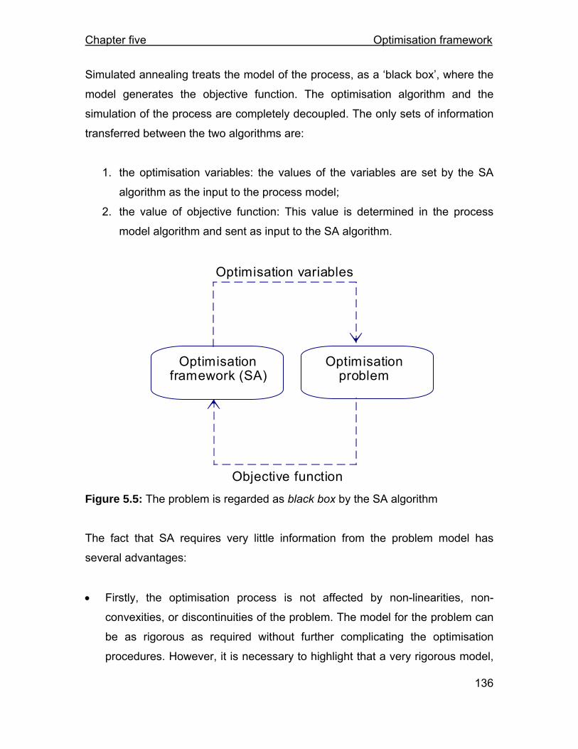
Chapter five Optimisation framework
136
Simulated annealing treats the model of the process, as a ‘black box’, where the
model generates the objective function. The optimisation algorithm and the
simulation of the process are completely decoupled. The only sets of information
transferred between the two algorithms are:
1. the optimisation variables: the values of the variables are set by the SA
algorithm as the input to the process model;
2. the value of objective function: This value is determined in the process
model algorithm and sent as input to the SA algorithm.
Optimisation variables
Objective function
Optimisationframework (SA)
Optimisationproblem
Figure 5.5: The problem is regarded as black box by the SA algorithm
The fact that SA requires very little information from the problem model has
several advantages:
• Firstly, the optimisation process is not affected by non-linearities, non-
convexities, or discontinuities of the problem. The model for the problem can
be as rigorous as required without further complicating the optimisation
procedures. However, it is necessary to highlight that a very rigorous model,

Chapter five Optimisation framework
137
with high computational time for the simulation, increases the optimisation
time significantly. Therefore, even though SA does not enforce limitations on
the simulation model of the problem, caution should still be exercised over
the level of the complexity of the process model.
• Secondly, as the optimisation algorithm and the problem to be optimised can
be completely decoupled, they can be implemented independently and even
in totally different environments or platforms (different programming
languages, for example).
• Thirdly, one generic optimisation algorithm can be developed and used to
optimise several optimisation problems.
The objective function applied in this work is described in section 5.5.
5.4.2.3 Acceptance Criteria
Acceptance criteria are the sets of rules on which basis a candidate solution is
accepted or rejected. The literature proposes several acceptance criteria
(Kirkpatrick et al., 1983; Glauber, 1963; Dueck and Scheuer, 1990; Hedar and
Fukushima, 2006; Pedamallu and Ozdamar, 2008).
As mentioned previously, SA accepts non-improving solutions with a probability.
Various formulations are proposed in the literature for calculating this probability.
However, the main parameters controlling the probability are the incremental
change in the objective function (∆F) and a user defined parameter, called the
annealing temperature (Ta). The probability is constructed in a way that the
higher the incremental change in the objective function (e.g. ∆F>>0, for a
minimisation problem), the lower the chance of accepting the solution will be.
Also, the annealing temperature controls the acceptance criteria so that the uphill
moves have a lower chance of acceptance when the annealing temperature is
low. For instance, in standard SA, the annealing temperature is high at the initial

Chapter five Optimisation framework
138
stages of optimisation and is reduced through the course of the optimisation.
Therefore, fewer candidate solutions associated with the uphill moves will be
accepted towards the end of the optimisation. In this work, the acceptance rules
are adopted from Pedamallu and Ozdamar (2008).
Acceptance criteria provide the opportunity to enhance the performance of
simulated annealing. These rules provide a diversified exploration in the search
space by also accepting the uphill moves. Accepting uphill moves assists SA not
to be trapped in the local optima. On the other hand, uphill moves are not always
accepted. In the present approach, the probability of accepting an uphill move is
calculated only if a certain number of candidate solutions, ELmin, are evaluated
and the last accepted solution is not improved. The probability is calculated using
Equation 5.5, (Pedamallu and Ozdamar, 2008).
exp (∆F / (fnew .Ta) if ∆f≥0
P = 5.5
1 if ∆f≤0
The value of the probability, P, is used to decide whether to accept a move or
not. If a randomly generated number is less than the calculated probability, P, the
uphill solution will be accepted. This procedure boosts the global search capacity
of the algorithm. A downhill move is always accepted. Each objective function is
compared with the previously accepted candidate solution to determine ∆F.
5.4.2.4 Annealing schedule
The annealing schedule consists of the choice of initial annealing temperature,
the number of solution candidates iterated at each temperature or epoch length,
the way in which annealing temperature is reduced and the final annealing
temperature. The annealing schedule that is used in this work is different from its
counterpart in standard SA.

Chapter five Optimisation framework
139
i. Initial annealing temperature The initial value of the annealing temperature affects the performance of the SA
algorithm significantly. The initial temperature, Tai, is set large enough to make
the probability of accepting all moves close to 1, each time the temperature is re-
initialised. If a very low temperature is chosen then the number of uphill moves
accepted will be reduced throughout the optimisation and the algorithm loses the
ability to escape from local optima.
Since the probability of acceptance, employed in this work (equation 5.5), is
based on a normalised deterioration, the initial annealing temperature is set to 1.
If, as in standard SA, Boltzmann factor is used (as the rejection criterion in
Metropolis algorithm), then as a rule of thumb, the Tai is set to be at least 10
times the maximum change in the value of the objective function between any
two successive moves. The maximum change in the objective function can be
estimated by simulating a number of possible trial solutions for the problem
(Athier et al., 1997).
ii. Epoch length In standard SA, at each temperature, a fixed number of candidate solutions are
evaluated. For each uphill move, the probability of accepting the candidate
solution is calculated and it is determined whether the candidate solution is
accepted or not. After the predetermined number of solutions are evaluated, the
annealing temperature is reduced. In other words, the epoch length is constant.
In the present approach, which is adopted from Hedar and Fukushima (2006),
and Pedamallu and Ozdamar (2008) an adaptive epoch length is chosen. In the
literature, this method has been tested against several SA algorithms and it is
claimed to be an effective approach (Demirhan and Ozdamar, 2000).
The annealing temperature is reduced each time an uphill move is accepted. An
uphill move may be accepted if a predetermined number (ELmin) of candidate
solutions are evaluated and none of them improves the last accepted solution. In

Chapter five Optimisation framework
140
other words, if ELmin -1 uphill moves are made consecutively, the ELmin uphill
solution is accepted with a probability. Each time a downhill move is made, the
counter value (EL) for non-improving (uphill) moves is re-initialised. So the
procedure will be as follows: at each annealing temperature, a counter, EL, is
initialised, which counts the number of candidate solutions. If a downhill solution
is found (relative to the last accepted solution), the counter is reset to zero or re-
initialised. Otherwise, if the counter EL reaches ELmin, the annealing temperature
is reduced and the counter EL is re-initialised.
Similar to the epoch length in the standard SA algorithm, the value of ELmin is
chosen to be a multiple of the problem dimension (i.e. number of optimisation
variables). This choice of ELmin should give a chance to all optimisation variables
to improve in the search neighbourhood (Pedamallu and Ozdamar, 2008). In this
work, ELmin is taken to be twice the dimension size of the problem.
iii. The schedule for temperature reduction Another factor that affects the performance of the SA optimiser is the way in
which the temperature is reduced. If the temperature is reduced too quickly, the
probability of accepting uphill moves reduces quickly through the course of
optimisation. Therefore, the algorithm has a lower chance of escaping local
minima. On the other hand, very slow cooling of the annealing temperature
increases the optimisation time unnecessarily.
The cooling schedule employed in the present work is given by Equation 5.6
(Aarts and Van Laarhoven, 1985). The speed of cooling is controlled by the
cooling parameter, θ. The bigger the value of θ, the faster the reduction of the
annealing temperature will be. This parameter takes values between 0 and 1,
with typical values around 0.05. The value of θ can be changed through the
optimisation to speed up or slow down the cooling process in different
optimisation stages. σ( T ka ) represents the standard deviation of the objective
Chapter five Optimisation framework
141
function of all the trial solutions generated at the temperature T ka . The inclusion
of this factor in the schedule has the effect of accelerating the cooling when the
standard deviation of the objective function is small.
1
ka
kak
a1k
a )T(3).ln(1T1T T
−
+⎥⎦
⎤⎢⎣
⎡
⋅+
+⋅=σ
θ 5.6
iv. Final annealing temperature It has been observed in the literature (Hedar and Fukushima, 2006) that setting
the final annealing temperature to the minimum of (10-5, 10-5 Tai) could allow
complete cooling. The probability of accepting uphill moves will be almost zero at
this temperature.
5.4.2.5 Multi-start algorithm
Another feature of the present SA algorithm, which differentiates it from the
standard SA, is that it has multiple starting points. Standard SA starts from an
initial point and all through the optimisation each candidate is generated by
making one change to the previous candidate solution. So, as shown in Figure
5.6-(a), a continuous search in the space is made. This continuous search may
fail to search all the solution space. In the present approach, however, the
optimiser may change its current solution point and carries out the optimisation
from different points, which are randomly selected within the search space,
Figure 5.6-(b). This strategy increases the chance of searching the solution
space more thoroughly.
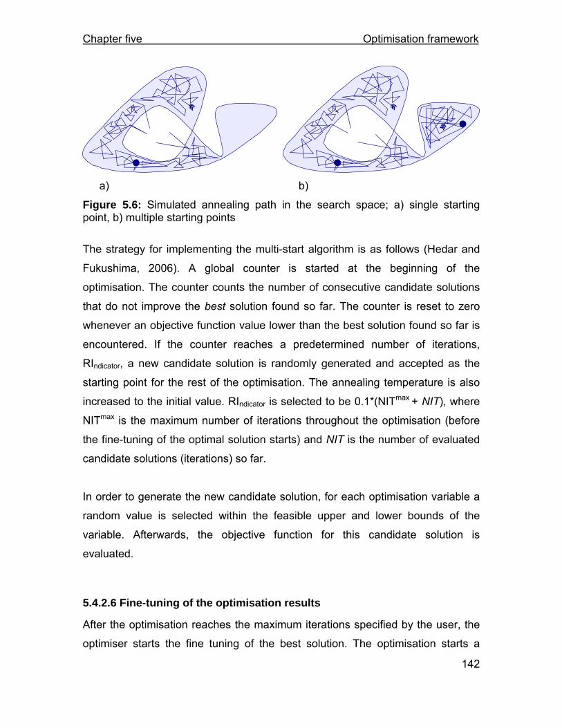
Chapter five Optimisation framework
142
a) b)
Figure 5.6: Simulated annealing path in the search space; a) single starting point, b) multiple starting points
The strategy for implementing the multi-start algorithm is as follows (Hedar and
Fukushima, 2006). A global counter is started at the beginning of the
optimisation. The counter counts the number of consecutive candidate solutions
that do not improve the best solution found so far. The counter is reset to zero
whenever an objective function value lower than the best solution found so far is
encountered. If the counter reaches a predetermined number of iterations,
RIndicator, a new candidate solution is randomly generated and accepted as the
starting point for the rest of the optimisation. The annealing temperature is also
increased to the initial value. RIndicator is selected to be 0.1*(NITmax + NIT), where
NITmax is the maximum number of iterations throughout the optimisation (before
the fine-tuning of the optimal solution starts) and NIT is the number of evaluated
candidate solutions (iterations) so far.
In order to generate the new candidate solution, for each optimisation variable a
random value is selected within the feasible upper and lower bounds of the
variable. Afterwards, the objective function for this candidate solution is
evaluated.
5.4.2.6 Fine-tuning of the optimisation results
After the optimisation reaches the maximum iterations specified by the user, the
optimiser starts the fine tuning of the best solution. The optimisation starts a

Chapter five Optimisation framework
143
series of moves from the point of the best solution found so far. The current
annealing temperature will be used as the initial annealing temperature and the
optimisation will be followed using the same cooling schedule. However, no re-
initialisation will be performed. This strategy will improve the local search around
the best solution found.
5.4.2.7 Termination Criteria
Several criteria for deciding when to terminate the search algorithm have been
proposed for standard SA (Rastogi, 2006). In the present formulation, the
optimisation search is terminated either:
• when twice the maximum number of candidate solutions, NITmax, have been
evaluated; or,
• the annealing temperature reaches its final value and more than NITmax
iterations have been evaluated.
5.4.2.8 Constraint handling
There are a number of approaches to account for the process constraints:
• Using penalty function
This is one of the most common approaches for handling the constraints in an
optimisation problem. A penalty value is added to the objective function when the
associated candidate solution violates the defined constraints. The literature
proposes many different ways of penalising the objective function (Michalewicz,
1994).
• Modifying the process formulation and candidate solution generation
The problem can be formulated in a way that unnecessary constraints are not
enforced on the optimizer. There are certain conditions that appear to the
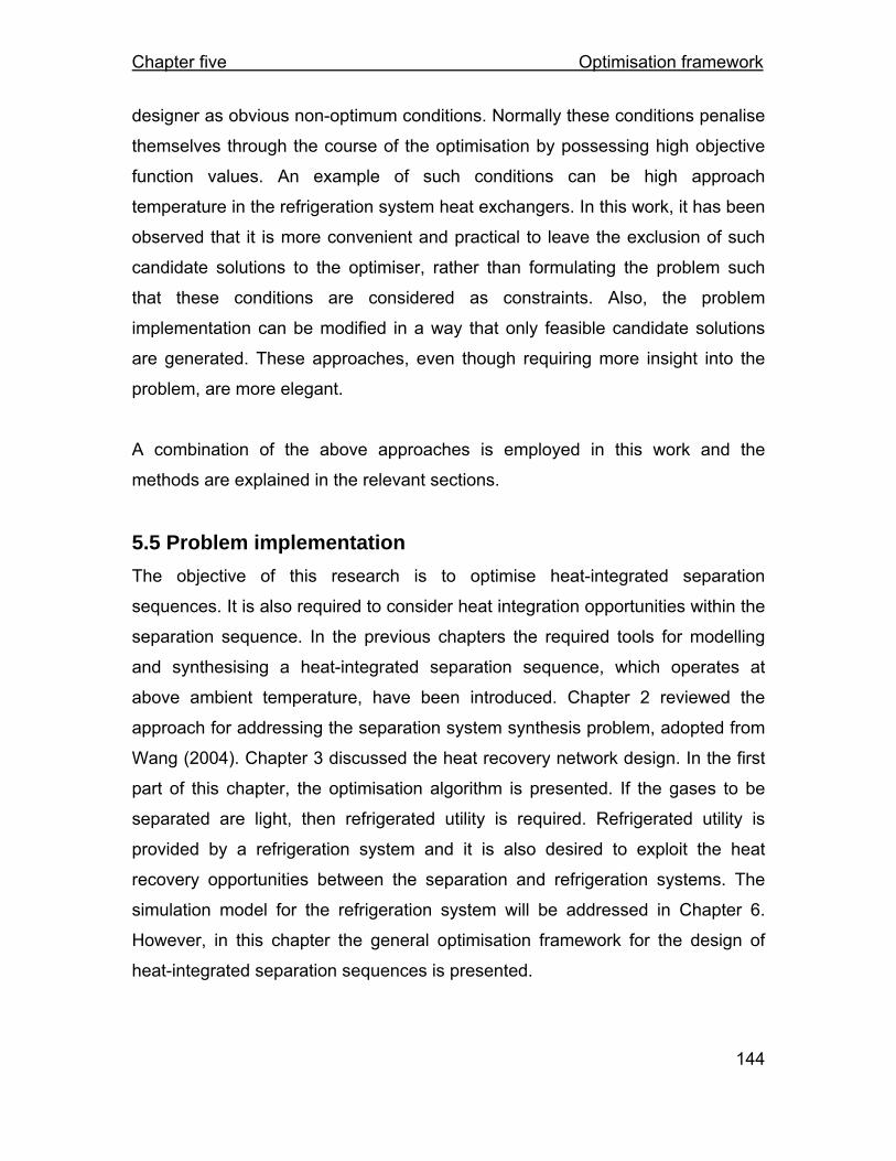
Chapter five Optimisation framework
144
designer as obvious non-optimum conditions. Normally these conditions penalise
themselves through the course of the optimisation by possessing high objective
function values. An example of such conditions can be high approach
temperature in the refrigeration system heat exchangers. In this work, it has been
observed that it is more convenient and practical to leave the exclusion of such
candidate solutions to the optimiser, rather than formulating the problem such
that these conditions are considered as constraints. Also, the problem
implementation can be modified in a way that only feasible candidate solutions
are generated. These approaches, even though requiring more insight into the
problem, are more elegant.
A combination of the above approaches is employed in this work and the
methods are explained in the relevant sections.
5.5 Problem implementation The objective of this research is to optimise heat-integrated separation
sequences. It is also required to consider heat integration opportunities within the
separation sequence. In the previous chapters the required tools for modelling
and synthesising a heat-integrated separation sequence, which operates at
above ambient temperature, have been introduced. Chapter 2 reviewed the
approach for addressing the separation system synthesis problem, adopted from
Wang (2004). Chapter 3 discussed the heat recovery network design. In the first
part of this chapter, the optimisation algorithm is presented. If the gases to be
separated are light, then refrigerated utility is required. Refrigerated utility is
provided by a refrigeration system and it is also desired to exploit the heat
recovery opportunities between the separation and refrigeration systems. The
simulation model for the refrigeration system will be addressed in Chapter 6.
However, in this chapter the general optimisation framework for the design of
heat-integrated separation sequences is presented.
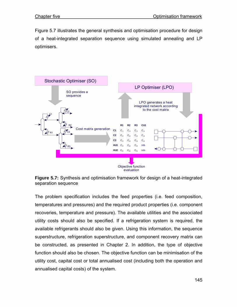
Chapter five Optimisation framework
145
Figure 5.7 illustrates the general synthesis and optimisation procedure for design
of a heat-integrated separation sequence using simulated annealing and LP
optimisers.
Stochastic Optimiser (SO)
C3R1
R3
R2
C1C2
R1 R2 R3 CU1
C1 C11 C12 C13 C14
C2 C21 C22 C23 C24
C3 C31 C32 C33 C34
HU1 C41 C42 C43 Infs
HU2 C51 C52 C53 Infs
SO provides asequence
Cost matrix generation
LPO generates a heatintegrated network according
to the cost matrix
Objective functionevaluation
LP Optimiser (LPO)
Figure 5.7: Synthesis and optimisation framework for design of a heat-integrated separation sequence
The problem specification includes the feed properties (i.e. feed composition,
temperatures and pressures) and the required product properties (i.e. component
recoveries, temperature and pressure). The available utilities and the associated
utility costs should also be specified. If a refrigeration system is required, the
available refrigerants should also be given. Using this information, the sequence
superstructure, refrigeration superstructure, and component recovery matrix can
be constructed, as presented in Chapter 2. In addition, the type of objective
function should also be chosen. The objective function can be minimisation of the
utility cost, capital cost or total annualised cost (including both the operation and
annualised capital costs) of the system.

Chapter five Optimisation framework
146
The equation of state should also be decided prior to the optimisation. In this
work, the Peng-Robinson equation of state is applied to calculate thermodynamic
properties.
The next step is to set up the optimisation conditions. The values for the
boundaries of the optimisation variables and the SA parameters (such as epoch
length and maximum number of iterations) are selected by the designer
according to the problem of interest.
Changing the SA optimisation variables forms the SA moves. Figure 5.8 shows
the corresponding moves for optimisation variables in the problem of design of
heat-integrated separation sequence.
Figure 5.8: Simulated annealing moves in optimisation of a heat-integrated separation sequence
After the starting point (initial design) is generated for simulated annealing, at
each optimisation step, SA performs one of the moves shown in Figure 5.8. The
Heat integrated distillation sequence moves
Distillation moves Refrigeration moves
Column 1
Column 2
Column 3
Column n
Task type
Sequence type
Column type
Column pressure
Column feed quality
Column condenser type
Cascade structure
Cycle 1
Cycle 2
Cycle 3
Cycle composition
Cycle pressure levels
P 1-P

Chapter five Optimisation framework
147
newly generated values of the optimisation variables are transferred to the
separation sequence simulation algorithm. This algorithm will simulate and
synthesise the separation sequence, and hence calculates the heating and
cooling demands of the process streams. The temperature and loads of process
streams, requiring heating and cooling, are sent to the heat recovery network
design algorithm. In an above ambient process, the cost matrix (Chapter 3) is
constructed and an LP optimiser is employed to optimise the loads in each
match. Basically, heat integration opportunities will be exploited and the suitable
utility will be allocated to the process streams. In a below-ambient separation
sequence, the refrigeration system is also synthesised and optimised, while the
cost matrix is constructed (see Chapter 6 for the refrigeration system synthesis
methodology). All the optimisation variables for the refrigeration system are
optimised by simulated annealing, except for the number of compression stages.
In order to control the complexity of the design, the number of compression
stages is controlled using binary variables. An MILP problem is optimised, which
minimises the loads on each match between the sources and the sinks in the
process and controls the number of refrigeration levels. The result of linear
optimisation will be the performance of heat exchanger network together with the
refrigeration system.
Thereafter, for the objective of minimum utility cost, the simulated sequence (and
refrigeration system in a sub-ambient process) is priced as:
Utility cost = Compressor power cost + Cold utility cost + Hot utility cost
Utility costs include the costs of utilities for condensers, reboilers, feed and
product heaters and coolers.
If the objective is to optimise the total annualised cost the capital cost of the
system should also be calculated. The capital cost will include the cost of

Chapter five Optimisation framework
148
separation devices, reboilers, condensers, heaters, coolers and compressors in
the process.
The objective function value is returned to the optimiser and this process is
repeated until the termination criterion is met. The optimisation algorithm
develops several prospective solutions for the problem under study, accepts and
rejects these solutions based on their performance with respect to the objective
function. Figure 5.9 shows the flow of information for the synthesis and
optimisation of a heat integrated separation sequence.
Figure 5.9: Flow of information in the optimisation framework
It should be noted that the separation sequence, the refrigeration system and
heat integration opportunities are being optimised simultaneously. The results
from these different parts of the process contribute to the overall objective
function, which is then evaluated and its value is fed back to the optimiser.
The problem simulation and optimisation framework presented in this work is
formulated in FORTRAN 77 program and embedded in the COLOM© software,
Problem specification
(MI)LP optimisation of heat recovery network (& simulation of the refrigeration system in a low temperature system)
Simulated annealing
Simulation of the separation sequence and economic evaluation of the design
Recovery matrix, separation sequence superstructure and refrigeration system database are built.
Process stream data
Optimisation variables for the separation sequence
Value of the objective function
Optimisation variables for the refrigeration system
Optimal solution
Heat recovery network and refrigeration system power demand

Chapter five Optimisation framework
149
part of the process design software suite available from the Centre for Process
Integration at the University of Manchester.
5.6 Case study - BTEXC 5.6.1 Introduction In this section, a case study is presented to illustrate the performance of the
proposed methodology for minimising the operating cost of heat integrated
separation sequences.
The mixture of aromatics in Table 5.1 is to be separated into the products
specified in the same table. The C9’s are to be represented by C9H12 (1-
methylethyl benzene). For a 5-product separation problem, 14 separation
sequences of simple columns are possible. Smith (2005 – Example 11.3) ranks
the order of the distillation sequences on the basis of total vapour load,
calculated from Underwood equations.
Table 5.1: Data for five-product mixture of aromatics to be separated by distillation
i Components in feed Mole fraction Product specification
A Benzene 0.31 100% recovery of benzene
B Toluene 0.32 100% recovery of Toluene
C Ethyl-benzene 0.07 100% recovery of Ethyl-benzene
p-Xylene 0.05
m-Xylene 0.13 100% recovery of Xylenes D
o-Xylene 0.07
E C9’s 0.05 100% recovery of C9’s
Flowrate 864.4 kmol/h, saturated liquid at 1.013 bar

Chapter five Optimisation framework
150
Table 5.2: Relative volatilities of the feed to the sequence at 1 atm
i Components in feed Relative volatility
A Benzene 7.577
B Toluene 3.245
C Ethyl-benzene 1.565
p-Xylene 1.467
D m-Xylene 1.417
o-Xylene 1.220
E C9’s 1.000
The outcome of the study of Smith (2005) is as follows. The relative volatilities of
the feed components shown in Table 5.2 suggest that the ethyl-benzene (C)/
xylenes (D) separation is by far the most difficult separation. Heuristic rules
suggest that such a difficult separation should be carried out in isolation from
other components. However, the results from studying the vapour loads in
columns by Smith (2005) show the contrary. The best two sequences in terms of
vapour load for the separation of the mixture of aromatics are shown in Figure
5.10. The difficult separation C\D is carried out in the presence of other
components. Smith (2005) reports that further investigations have shown that the
relative volatility of the difficult separation is sensitive to the presence of other
components. The presence of other feed components increases slightly the
relative volatility of the C/D separation, making it beneficial to carry out C/D
separation in the presence of other feed components. Smith (2005) notes that
the use of total vapour flow is only a guide in screening separation sequences
and suggests the calculations being taken one step further to calculate the
energy costs. Obviously, in the study of Smith (2005), the heat integration
opportunities are not considered and the column pressures are fixed at
atmospheric conditions.
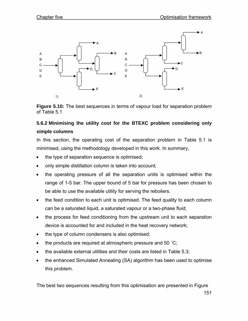
Chapter five Optimisation framework
151
Figure 5.10: The best sequences in terms of vapour load for separation problem of Table 5.1 5.6.2 Minimising the utility cost for the BTEXC problem considering only simple columns In this section, the operating cost of the separation problem in Table 5.1 is
minimised, using the methodology developed in this work. In summary,
• the type of separation sequence is optimised;
• only simple distillation column is taken into account;
• the operating pressure of all the separation units is optimised within the
range of 1-5 bar. The upper bound of 5 bar for pressure has been chosen to
be able to use the available utility for serving the reboilers.
• the feed condition to each unit is optimised. The feed quality to each column
can be a saturated liquid, a saturated vapour or a two-phase fluid;
• the process for feed conditioning from the upstream unit to each separation
device is accounted for and included in the heat recovery network;
• the type of column condensers is also optimised;
• the products are required at atmospheric pressure and 50 ˚C;
• the available external utilities and their costs are listed in Table 5.3;
• the enhanced Simulated Annealing (SA) algorithm has been used to optimise
this problem.
The best two sequences resulting from this optimisation are presented in Figure
A
B
C
D
E
A
B
CD
E
A
B
C
D
E
A
B
C
D
E
1) 2)
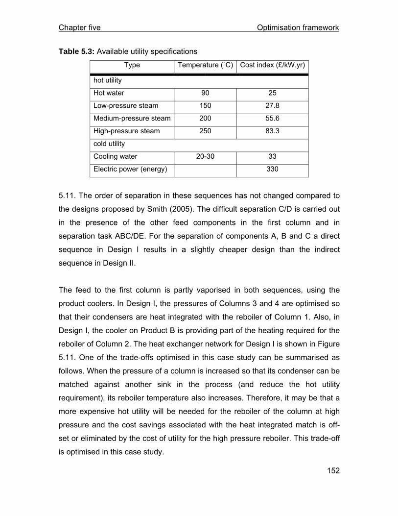
Chapter five Optimisation framework
152
Table 5.3: Available utility specifications
Type Temperature (˚C) Cost index (£/kW.yr)
hot utility
Hot water 90 25
Low-pressure steam 150 27.8
Medium-pressure steam 200 55.6
High-pressure steam 250 83.3
cold utility
Cooling water 20-30 33
Electric power (energy) 330
5.11. The order of separation in these sequences has not changed compared to
the designs proposed by Smith (2005). The difficult separation C/D is carried out
in the presence of the other feed components in the first column and in
separation task ABC/DE. For the separation of components A, B and C a direct
sequence in Design I results in a slightly cheaper design than the indirect
sequence in Design II.
The feed to the first column is partly vaporised in both sequences, using the
product coolers. In Design I, the pressures of Columns 3 and 4 are optimised so
that their condensers are heat integrated with the reboiler of Column 1. Also, in
Design I, the cooler on Product B is providing part of the heating required for the
reboiler of Column 2. The heat exchanger network for Design I is shown in Figure
5.11. One of the trade-offs optimised in this case study can be summarised as
follows. When the pressure of a column is increased so that its condenser can be
matched against another sink in the process (and reduce the hot utility
requirement), its reboiler temperature also increases. Therefore, it may be that a
more expensive hot utility will be needed for the reboiler of the column at high
pressure and the cost savings associated with the heat integrated match is off-
set or eliminated by the cost of utility for the high pressure reboiler. This trade-off
is optimised in this case study.

Chapter five Optimisation framework
153
Design I
Condenser Reboiler Column Pressure
(bar)
Feed
quality ˚C MW ˚C MW
Condenser
type
1 1 0.9 104 23.5 142 30.3 Pc
2 1 0.2 80 8.2 114 4.8 Tc
3 1.5 0.1 156 11.7 169 9.5 Tc
4 2.9 0.1 153 7 181 4.7 Tc
Objective value: 3.1 MM£/yr
R1 R2
1 3
C1
C3
2 5 6 7 8 9
4
C2
C4
R4 R3
5
1
2
3
41
2
3
4
6
78
9
C1
R1
R2
C3
R3
C4
R4
C2
A
B
CD
E

Chapter five Optimisation framework
154
Design II
Figure 5.11: Selected designs for BTEXC problem of Table 5.1 considering only simple columns
Condenser Reboiler Column Pressure
(bar)
Feed
quality ˚C MW ˚C MW
Condenser
type
1 1 0.8 104 24.2 142 30 Pc
2 1 0 92 9.2 136 4.2 Tc
3 1.4 0.1 151 11.6 164 9.4 Tc
4 1 0 80 6.3 111 4.3 Pc
Objective value: 3.3 MM£/yr
1
2
3
4
1
2
3
4
5
6
7
8
9
C1
R1
C2
R2
C3
R3
C4
R4
A
B
C
D
R1 R2 R3
1
C1 C2 C3 C4 2 6 7 8 9
4
R4
3
5
E
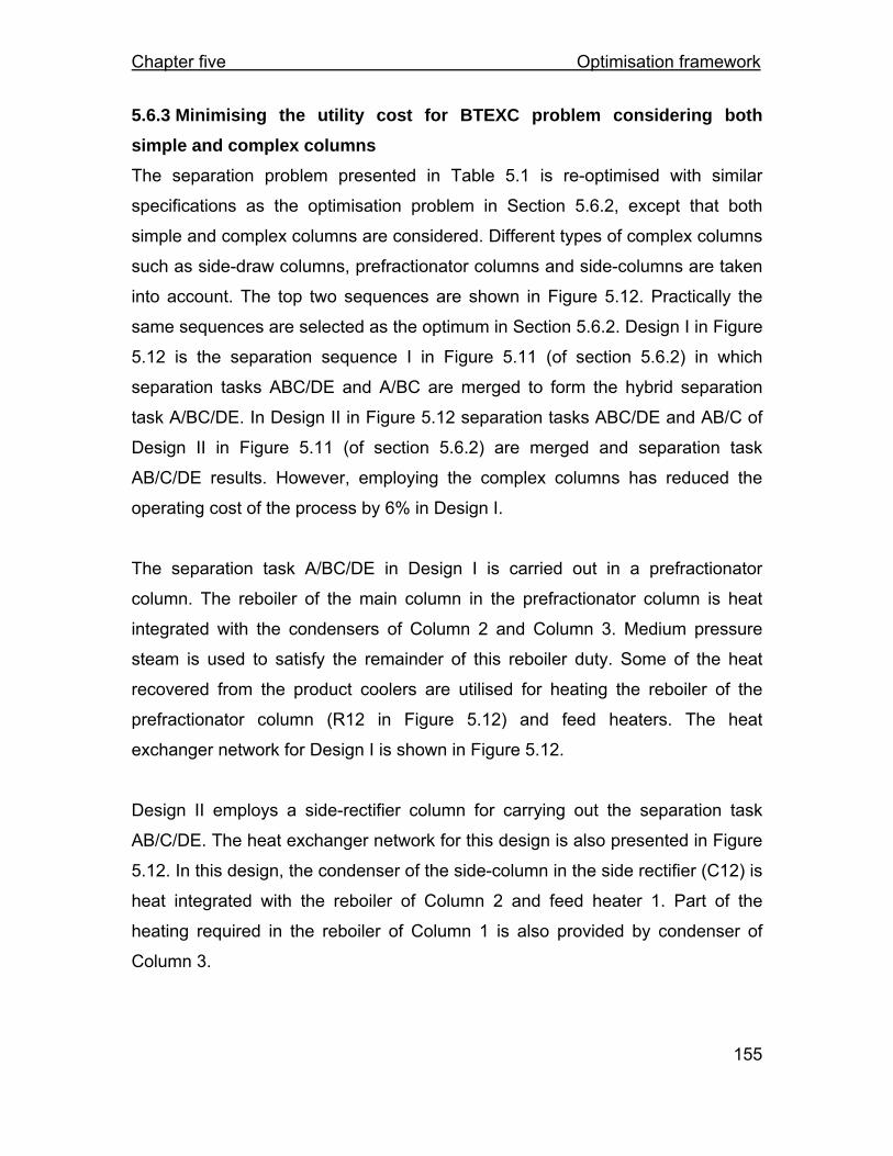
Chapter five Optimisation framework
155
5.6.3 Minimising the utility cost for BTEXC problem considering both simple and complex columns The separation problem presented in Table 5.1 is re-optimised with similar
specifications as the optimisation problem in Section 5.6.2, except that both
simple and complex columns are considered. Different types of complex columns
such as side-draw columns, prefractionator columns and side-columns are taken
into account. The top two sequences are shown in Figure 5.12. Practically the
same sequences are selected as the optimum in Section 5.6.2. Design I in Figure
5.12 is the separation sequence I in Figure 5.11 (of section 5.6.2) in which
separation tasks ABC/DE and A/BC are merged to form the hybrid separation
task A/BC/DE. In Design II in Figure 5.12 separation tasks ABC/DE and AB/C of
Design II in Figure 5.11 (of section 5.6.2) are merged and separation task
AB/C/DE results. However, employing the complex columns has reduced the
operating cost of the process by 6% in Design I.
The separation task A/BC/DE in Design I is carried out in a prefractionator
column. The reboiler of the main column in the prefractionator column is heat
integrated with the condensers of Column 2 and Column 3. Medium pressure
steam is used to satisfy the remainder of this reboiler duty. Some of the heat
recovered from the product coolers are utilised for heating the reboiler of the
prefractionator column (R12 in Figure 5.12) and feed heaters. The heat
exchanger network for Design I is shown in Figure 5.12.
Design II employs a side-rectifier column for carrying out the separation task
AB/C/DE. The heat exchanger network for this design is also presented in Figure
5.12. In this design, the condenser of the side-column in the side rectifier (C12) is
heat integrated with the reboiler of Column 2 and feed heater 1. Part of the
heating required in the reboiler of Column 1 is also provided by condenser of
Column 3.

Chapter five Optimisation framework
156
Design I
Condenser Reboiler Column Pressure
(bar)
Feed
quality ˚C MW ˚C MW
Condenser
type
80 27 142 28.6 1 1
1
91 2 126 5.4
Tc
2 2.9 0.1 152 7 180 4.5 Tc
3 1.8 0.1 164 11.8 177 9.6 Tc
Objective value: 2.9 MM£/yr
5
C3
3
C1
R1 R12
4
C2
R2 R3 1 2
6 7 8
C12
1 2
3
1 2
3
4
57
8
C1
R1
C2
R2C3
R3
C12
R12
6
1: Prefractionator column
A B
CD
E

Chapter five Optimisation framework
157
Design II
Figure 5.12: Selected designs for BTEXC problem of Table 5.1 considering both simple and complex columns
Condenser Reboiler Column Pressure
(bar)
Feed
quality ˚C MW ˚C MW
Condenser
type
99 7.9 Pc 1
1
0
136 25.8
142
32.3
Tc
2 1 0.1 80 6.1 111 4.4 Pc
3 1.4 0 152 11.7 164 9.3 Tc
Objective value: 2.9 MM£/yr
6
1
2
3
1
2
3
4
5
7
C1
R1
C2
R2
C3
R3
C12
1: Side rectifier column
A
BC
D
5
C3
C1
R1
4
C2
R2 R3 1 3
6 7 2
C12
E
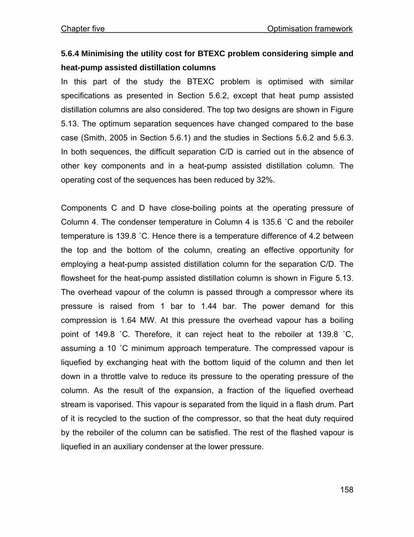
Chapter five Optimisation framework
158
5.6.4 Minimising the utility cost for BTEXC problem considering simple and heat-pump assisted distillation columns In this part of the study the BTEXC problem is optimised with similar
specifications as presented in Section 5.6.2, except that heat pump assisted
distillation columns are also considered. The top two designs are shown in Figure
5.13. The optimum separation sequences have changed compared to the base
case (Smith, 2005 in Section 5.6.1) and the studies in Sections 5.6.2 and 5.6.3.
In both sequences, the difficult separation C/D is carried out in the absence of
other key components and in a heat-pump assisted distillation column. The
operating cost of the sequences has been reduced by 32%.
Components C and D have close-boiling points at the operating pressure of
Column 4. The condenser temperature in Column 4 is 135.6 ˚C and the reboiler
temperature is 139.8 ˚C. Hence there is a temperature difference of 4.2 between
the top and the bottom of the column, creating an effective opportunity for
employing a heat-pump assisted distillation column for the separation C/D. The
flowsheet for the heat-pump assisted distillation column is shown in Figure 5.13.
The overhead vapour of the column is passed through a compressor where its
pressure is raised from 1 bar to 1.44 bar. The power demand for this
compression is 1.64 MW. At this pressure the overhead vapour has a boiling
point of 149.8 ˚C. Therefore, it can reject heat to the reboiler at 139.8 ˚C,
assuming a 10 ˚C minimum approach temperature. The compressed vapour is
liquefied by exchanging heat with the bottom liquid of the column and then let
down in a throttle valve to reduce its pressure to the operating pressure of the
column. As the result of the expansion, a fraction of the liquefied overhead
stream is vaporised. This vapour is separated from the liquid in a flash drum. Part
of it is recycled to the suction of the compressor, so that the heat duty required
by the reboiler of the column can be satisfied. The rest of the flashed vapour is
liquefied in an auxiliary condenser at the lower pressure.

Chapter five Optimisation framework
159
In Design I, separation sequence AB/CDE, CD/E, A/B, and C/D has been
selected. The feed to the first column has been partially vaporised using the
auxiliary condenser of the heat pump-assisted distillation column and low-
pressure steam. The reboiler of column 1 is served by the condenser of Column
3. Also, the condenser of Column 3 is partially heating the reboiler of Column 2.
The rest of heating required by the reboiler of Column 2 is supplied by the feed
cooler 6, which is providing a two-phase feed for the heat pump-assisted
distillation column. The rest of heat exchangers use external utilities. The heat
exchanger network for Design I is shown in Figure 5.13.
In Design II, separation sequence A/BCDE, B/CDE, CD/E and C/D has been
chosen. The reboiler of Column 2 is fully heat-integrated with the condenser of
Column 3. The condenser of Column 3 also provides part of the heating required
for the reboiler of Column 1. Stream cooler 5 and low-pressure steam are used
for providing the heating required in the reboiler of Column 1. The condenser of
Column 4 and the product cooler partially vaporise the feed to Column 1. The
rest of the heat exchangers use external utility, as shown in Figure 5.13.

Chapter five Optimisation framework
160
Design I
Condenser Reboiler Column Pressure
(bar)
Feed
quality ˚C MW ˚C MW
Condenser
type
1 1 0.6 99 5.4 140 8.3 Pc
2 1 0.1 80 8.4 110 4.4 Tc
3 1.5 0.8 155 10.4 168 12.5 Pc
4 1 0.7 136 1.6 - - Tc
Objective value: 1.9 MM£/yr
5
2
C1
R1
4
C4
R2 R3 1 3
6 7 8
C2
C3
1
2
3
4
1
2
3
4
5
6
7
C1
R1
C2
R2
C3
R3
8
C4
4: Heat pump assisted distillation column
A
B
E
C
D
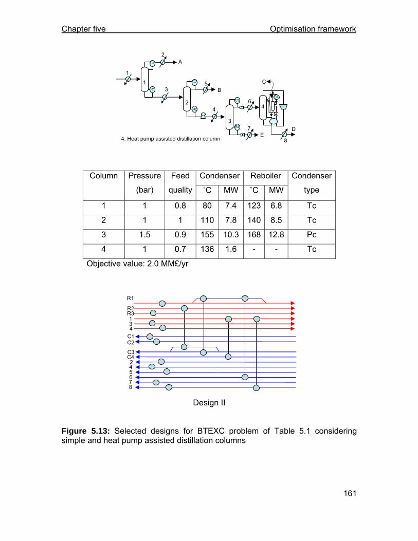
Chapter five Optimisation framework
161
Design II
Figure 5.13: Selected designs for BTEXC problem of Table 5.1 considering simple and heat pump assisted distillation columns
Condenser Reboiler Column Pressure
(bar)
Feed
quality ˚C MW ˚C MW
Condenser
type
1 1 0.8 80 7.4 123 6.8 Tc
2 1 1 110 7.8 140 8.5 Tc
3 1.5 0.9 155 10.3 168 12.8 Pc
4 1 0.7 136 1.6 - - Tc
Objective value: 2.0 MM£/yr
1
2
3
4
1
2
3
4
5
6
7
C1
R1
C2
R2
C3
R3
C4
84: Heat pump assisted distillation column
A
BC
D E
5
2
C1
R1
4
C4
R2 R3 1 3
6 7 8
C2
C3
4
Chapter five Optimisation framework
162
5.6.5 Minimising the utility cost for BTEXC problem considering simple, complex and heat-pump assisted distillation columns In this study further reduction in the operating cost has been observed as a result
of considering simple, complex and heat-pump assisted distillation columns. The
optimum sequence is shown in Figure 5.14. This sequence is composed of the
following separation tasks: A/B/CDE, CD/E, and C/D. The hybrid task A/B/CDE
is carried out in a prefractionator column and a heat pump-assisted distillation
column is used for the difficult separation C/D. The pressure of Column 2 has
been optimised so that the condenser of this column supplies the heating
required for the reboilers of the prefractionator column. A stream cooler 5 is also
providing some of the heating required for the reboiler of the prefractionator
column (R12) and the heating load of stream heater 1. The heat exchanger
network for this design is shown in Figure 5.14.
Condenser Reboiler Column Pressure
(bar)
Feed
quality ˚C MW ˚C MW
Condenser
type
80 8.2 140 6.2 1
1
1
90 2.1 126 5.6
Tc
2 1.5 0.9 156 10.3 169 13 Pc
3 1 0.9 136 1.2 - - Tc
Objective value: 1.8 MM£/yr
1
2
1 3
2
4
5
6
C1
R1C2
R2
C12
R12
C3
7
3
1: Prefractionator
4: Heat pump assisted distillation column
AB
C
D
E

Chapter five Optimisation framework
163
Figure 5.14: Selected designs for BTEXC problem of Table 5.1 considering simple, complex, and heat pump assisted distillation columns
5.6.6 Case study summary Table 5.4 summarises the results of BTEXC problem optimisation. In each
scenario, the best heat integrated separation sequences are screened among
various optimisations. The case study shows the flexibility of the present model
for carrying out various process investigations at the conceptual design stage.
Moreover, application of the heat pump assisted distillation columns at above
ambient temperature has also been demonstrated. The results show that
applying heat pump assisted distillation columns changes the order of
separation, while introducing energy savings in the process.
Table 5.4: BTEXC case study summary
Scenario Objective value (MM£/yr) Performance
Simple columns 3.1 100%
Simple + complex columns 2.9 93%
Simple + heat pump assisted distillation columns
1.9 61%
Simple + heat pump assisted + complex columns
1.8 58%
The SA parameters and the optimisation time for different parts of the presented
study are summarised in Table 5.5. It should be noted that the reason for higher
C3
1
5
3
C1
R1
4
R12 R2
6 7
C12
C2
2

Chapter five Optimisation framework
164
optimisation time in the case of simple and heat pump assisted distillation column
is the higher computational time for heat pumped columns due to the iterative
procedure for calculating the composition of the inlet stream to the compressor.
In the case of simple and heat pump assisted distillation column, it is expected
that more heat pumped columns to be calculated.
Table 5.5: SA parameters for BTEXC case study
SA Parameters
Case study scenarios ELmin NITmax i
aT Time
Simple columns 10 2000 0.05 37 minutes
Simple + complex columns 15 2000 0.05 29 minutes
Simple + heat pump assisted distillation columns 10 2000 0.05 67 minutes
Simple + heat pump assisted + complex columns 15 3000 0.05 44 minutes
5.7 Summary The synthesis and optimisation methodology for heat integrated separation
sequences has been presented in this chapter. An enhanced simulated
annealing algorithm has also been described. In this work, the enhanced
simulated annealing uses the process simulation models in Chapters 2 to 4 to
optimise a heat integrated separation sequence. A case study was presented in
order to demonstrate the performance of the synthesis and optimisation
approach in this work.
5.8 Nomenclature a Lower bound for a continuous optimisation variable
b Upper bound for a continuous optimisation variable
EL Counter for the epoch length
ELmin Minimum epoch length
m Lower bound for a discrete optimisation variable
n Upper bound for a discrete optimisation variable
Chapter five Optimisation framework
165
NIT Number of iterations
NITmax Maximum number of iterations before fine-tuning the optimal
solution
F(x) Value of objective function
fnew The objective function value for the newly calculated candidate
solution
k Counter of annealing temperatures
Lm Counter for epoch length
P Probability of a simulated annealing move
RIndicator The number which determines when to re-initialise the
optimisation procedure
Ta Annealing temperature
Tai Initial annealing temperature
x Set of variables for the optimisation problem
X Continuous optimisation variables
Y Discrete optimisation variables
Greek letters ∆ Incremental change in the variable
ω A random number between 0 and 1
θ Cooling parameter for the annealing temperature
σ the standard deviation of the objective function of all the trial
solutions generated at the temperature T ka

Chapter six Refrigeration system design in low temperature separation sequences
166
6 Chapter Six Refrigeration system design in Low-temperature separation sequences
6.1 Introduction Distillation is a competitive process for separating the components of a gas
mixture such as natural gas or the effluent of the reactor in an olefins plant. Such
processes demand utility at below-ambient temperatures. Hence, refrigeration
systems should be provided for such processes. Refrigeration systems in gas
separation plants account for a large percentage of the capital and operating
costs. To purify the components of a light hydrocarbon-mixture economically,
reliably, and environmentally benign, efficient separation equipment with the
appropriate operating conditions should be selected throughout the separation
train. This requires integration to reduce the primary energy consumption of the
system and optimise the quality of the required energy.
The objective of the present work is to screen separation sequences †† that
require refrigeration. Also, it is desired that in the screening procedure, some
insights regarding the structure and operating conditions of the refrigeration
system are derived. Therefore, a robust tool should be developed to design and
evaluate the performance of the refrigeration system where the tool maintains the
following characteristics:
1. The design methodology should embed various options for the design of
the refrigeration system processes. Examples of such options include:
type of refrigerant or the structure of the refrigeration system.
†† Screening separation sequences in a process refers to design and evaluation of the performance of various separation options. The performance of a separation sequence can be assessed in different ways. For instance, calculating the operating cost of the process can show the economic performance of the process from energy point of view.

Chapter six Refrigeration system design in low temperature separation sequences
167
2. The refrigeration system design should be practical. For instance, a
system with too many refrigeration levels will not be an economically
viable design, even if it is technically feasible.
3. Heat integration opportunities between the refrigeration process and the
background system should be created and exploited by the methodology.
4. A simultaneous design of refrigeration system and the background
process is required. For instance, in this work, the intention is to design
and optimise the separation and the refrigeration system simultaneously.
In the previous chapters, a robust methodology for synthesis and optimisation of
heat integrated separation sequences at above-ambient temperatures was
introduced. In this chapter the methodology is extended to consider the
separation sequences at below-ambient temperature. First, a general discussion
is carried out on different types of refrigeration systems. Next, the importance of
simultaneous design of separation system and refrigeration system is discussed
and illustrated in an example. Then a methodology for evaluating and optimising
the performance of the refrigeration system, while optimising the corresponding
separation sequence is presented. This strategy is applied to two industrial case
studies in Chapter 7, demonstrating its effectiveness to exploit the interactions
between the separation and refrigeration systems systematically.
6.2 Low-temperature separation sequence A separation sequence is considered low-temperature if it requires utility at sub-
ambient temperatures for cooling and condensation. Examples of processes
involving low temperature distillation are ethylene plants, liquefied natural gas
(LNG) plants and air separation facilities. Ethylene and LNG plants need to cool
and liquefy light hydrocarbons, which have low critical temperatures and
pressures. An air separation plant purifies oxygen, nitrogen and argon by
distillation. These components also have low critical properties and sub-ambient
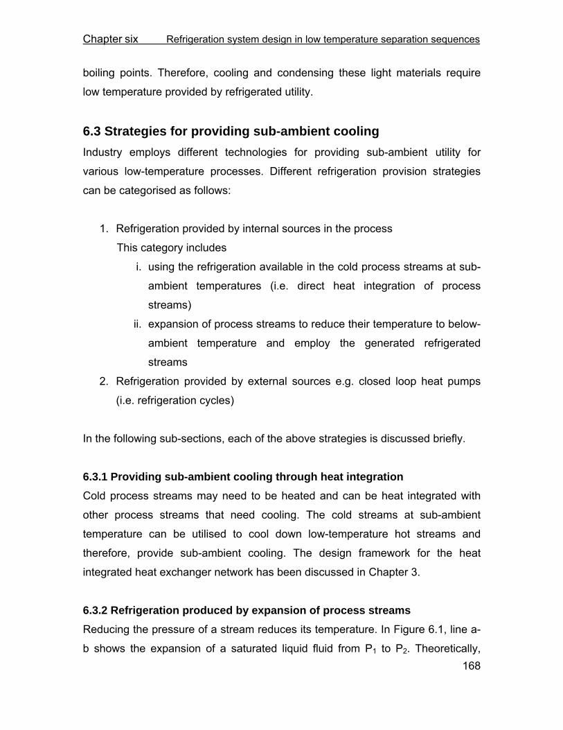
Chapter six Refrigeration system design in low temperature separation sequences
168
boiling points. Therefore, cooling and condensing these light materials require
low temperature provided by refrigerated utility.
6.3 Strategies for providing sub-ambient cooling Industry employs different technologies for providing sub-ambient utility for
various low-temperature processes. Different refrigeration provision strategies
can be categorised as follows:
1. Refrigeration provided by internal sources in the process
This category includes
i. using the refrigeration available in the cold process streams at sub-
ambient temperatures (i.e. direct heat integration of process
streams)
ii. expansion of process streams to reduce their temperature to below-
ambient temperature and employ the generated refrigerated
streams
2. Refrigeration provided by external sources e.g. closed loop heat pumps
(i.e. refrigeration cycles)
In the following sub-sections, each of the above strategies is discussed briefly.
6.3.1 Providing sub-ambient cooling through heat integration Cold process streams may need to be heated and can be heat integrated with
other process streams that need cooling. The cold streams at sub-ambient
temperature can be utilised to cool down low-temperature hot streams and
therefore, provide sub-ambient cooling. The design framework for the heat
integrated heat exchanger network has been discussed in Chapter 3.
6.3.2 Refrigeration produced by expansion of process streams Reducing the pressure of a stream reduces its temperature. In Figure 6.1, line a-
b shows the expansion of a saturated liquid fluid from P1 to P2. Theoretically,

Chapter six Refrigeration system design in low temperature separation sequences
169
pressure reduction can be carried out through an isenthalpic (i.e. constant
enthalpy) or isentropic process (i.e. constant entropy) process. Isenthalpic and
isentropic pressure drop are performed in a throttle valve and turbo-expander;
respectively.
Figure 6.1: T-H curve for an isenthalpic expansion
The temperature drop resulting from the stream pressure drop is employed in the
low-temperature processes to produce refrigeration. When the process is being
optimised, there are instances in which the optimum pressures of unit operations
dictate a pressure drop from the upstream to the downstream. This opportunity
can be employed to generate almost free refrigeration. In other words, almost no
energy is consumed for providing this refrigeration. At the conceptual design
stage, different pressure drop scenarios can be considered to exploit the trade-
offs between the performance of separation system and opportunities for
generating refrigeration.
6.3.3 Closed loop heat pump systems or compression refrigeration processes a. Simple cycles Figure 6.2-(a) illustrates an example of a simple refrigeration cycle (ETSU, 1992).
The cycle fluid or refrigerant at Point 2 is vaporised in an evaporator, absorbing
heat from the process stream. Through the evaporation process, the refrigerant
will provide cooling required in the process. The pressure of the saturated vapour
Lines of constant pressure a
b
T
H
P1
P2
Constant enthalpy
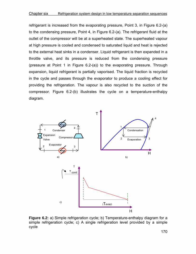
Chapter six Refrigeration system design in low temperature separation sequences
170
refrigerant is increased from the evaporating pressure, Point 3, in Figure 6.2-(a)
to the condensing pressure, Point 4, in Figure 6.2-(a). The refrigerant fluid at the
outlet of the compressor will be at a superheated state. The superheated vapour
at high pressure is cooled and condensed to saturated liquid and heat is rejected
to the external heat sinks in a condenser. Liquid refrigerant is then expanded in a
throttle valve, and its pressure is reduced from the condensing pressure
(pressure at Point 1 in Figure 6.2-(a)) to the evaporating pressure. Through
expansion, liquid refrigerant is partially vaporised. The liquid fraction is recycled
in the cycle and passes through the evaporator to produce a cooling effect for
providing the refrigeration. The vapour is also recycled to the suction of the
compressor. Figure 6.2-(b) illustrates the cycle on a temperature-enthalpy
diagram.
Figure 6.2: a) Simple refrigeration cycle; b) Temperature-enthalpy diagram for a simple refrigeration cycle; c) A single refrigeration level provided by a simple cycle
H
2 Evaporation
Condensation
3
4
b)
1
T
H
T
T
(Tevap)
cond
c)
4
3 2
Expansion
Valve Compressor
Condenser
Evaporator
1
a)

Chapter six Refrigeration system design in low temperature separation sequences
171
Another class of simple cycles is a turbo-expander cycle. In this type of cycle, the
expansion process is carried out in a turbo-expander instead of a throttle valve.
In such cycles, the turbo-expander not only expands and reduces the
temperature of the high pressure refrigerant fluid, but also produces work. This
work is often used to drive the compressor (Bloch and Soares, 2001; Kerry,
2007; Flynn, 2004).
In the present study, the refrigeration provided by a turbo-expander through the
expansion of a process stream (section 6.3.2) is accounted for. However, a
simple cycle that uses a turbo expander instead of a throttle valve will not be
considered and is recommended as part of future work.
b. Complex refrigeration cycles Simple refrigeration cycles can be used to provide cooling as low as -40˚C (Smith
2005). For lower temperatures, complex refrigeration cycles are normally used.
In this text, cycles with multistage compression and/or expansion and cascaded
systems are referred to as complex refrigeration systems.
i. Multistage cycles When cooling is required over a wide temperature range, employing a multistage
refrigeration cycle reduces the power requirement compared with a single-level
refrigeration cycle (Smith, 2005). A multistage cycle features more than one
evaporating stage. Each evaporating stage in a complex cycle will have a
different pressure and/or fluid composition. Figure 6.3-(a) shows a multistage
refrigeration cycle with each refrigeration level at a different pressure.
Figure 6.3-(b) shows the overall temperature-enthalpy (T-H) profile (i.e.
combined T-H profiles for all refrigeration stages) for the refrigeration system of
Figure 6.3-(a), when the cycle fluid is a mixture. Figure 6.3-(c) presents the
overall T-H profile for the cycle of Figure 6.3-(a) if the cycle fluid is a pure
component.

Chapter six Refrigeration system design in low temperature separation sequences
172
a)
P 1
P 2
P 4
P 1
P 2
P 3
P 3
P 4
(T ev ap)1
(T ev ap)2
(T ev ap)3
Tc ond
b)
(Tevap)1
(Tevap)2
Tcond
(Tevap)3
H
T
c)
(Tevap)1
(Tevap)2
(Tevap)3
Tcond
H
T
Figure 6.3: a) Multistage refrigeration cycle with multiple pressure levels; b) temperature-enthalpy diagram for cycle (a) with a mixed refrigerant; c) temperature-enthalpy diagram for cycle (a) with a pure refrigerant
Figure 6.4-(a) shows another type of multistage refrigeration system (Del Nogal,
2006). In this multistage refrigeration cycle, a mixture of fluid is used as the cycle
fluid and different refrigeration levels are generated by cooling the cycle fluid to
different temperatures. Thereafter, the cycle fluid is expanded to a single
pressure. It should be noted that the refrigeration levels are at the same
pressure. The different temperature at each level is mainly the result of the
different cycle fluid composition at each level.

Chapter six Refrigeration system design in low temperature separation sequences
173
P2
P1, T2, X2
P2
P2
P1, T1, X1
P1, T3, X3
P2
(Tevap)1
(Tevap)2
(Tevap)3
(Tevap)1
(Tevap)2
(Tevap)3
H
T
a) b)
Figure 6.4: a) Multistage refrigeration cycle with multiple temperature levels and a single pressure level; b) temperature-enthalpy diagram for cycle (a)
In all the above multistage refrigeration systems, different temperature levels will
be generated, which allows a close match between the temperature-enthalpy
curve of the process (when the curve is sloped) and of the refrigerant streams.
Therefore, the power required (for serving the process streams shown in the
above Figures) is less than when using a single-level system (Figure 6.2-(c)), as
a smaller temperature lift‡‡ is needed by the higher temperature levels (Smith,
2005).
A multistage cycle can also have more than one condensing stage at different
pressures. A cycle with multiple condensing stages can reject heat to multiple
process sinks in the background process. If the process sinks are at sub-ambient
temperatures, a reduction in power consumption will be acheived. In other words,
a refrigeration system with multiple rejection levels (in which all rejection levels,
but at most one, are at sub-ambient temperature) is expected to require less
power compared to a system that rejects all the heat to the ambient utility.
‡‡ The temperature lift is the temperature difference between the source and the sink streams, between which the refrigeration system operates, plus the minimum temperature approaches in the evaporator and condenser of the refrigeration cycle.

Chapter six Refrigeration system design in low temperature separation sequences
174
ii. Cascaded cycles A cascaded system comprises of two or more refrigeration cycles linked together.
Each cycle employs a different refrigerant. Figure 6.5 illustrates a cascaded
refrigeration process involving two simple cycles. The lower cycle extracts heat at
temperature Tevap and lifts it to the temperature Tcond1. The upper cycle
accepts the heat at temperature Tevap1 and pumps the heat at temperature
Tcond to an external heat sink.
Figure 6.5: Cascaded refrigeration cycles
There are two situations in which a cascaded refrigeration system should be
considered (Lee, 2001). Firstly, when any single refrigerant cannot cover a wide
temperature range between evaporation and condensation, a cascaded system
can be employed. Secondly, it might be applied when using a single refrigeration
cycle consumes more shaft power than a cascaded cycle.
Different arrangements of cascaded refrigeration cycles are employed in
industry:
• Cascades of cycles with pure refrigerants
e.g. ConocoPhillips Optimized Cascade
• Cascades of cycles with mixed refrigerants
Tevap
Tevap1
Tcond1
Lower cycle
Upper cycle
Tcond

Chapter six Refrigeration system design in low temperature separation sequences
175
e.g. Dual MR cycle by Shell
• Cascades of pure and mixed refrigerants
e.g. APCI’s Propane Pre-cooled process
6.4 Selection of refrigerant for compression refrigeration system A refrigerant is the fluid in the refrigeration cycle that exchanges heat with the
process streams. The refrigerant can be a pure component (referred to as pure
refrigerant) or a mixture of different components (referred to as mixed
refrigerant).
6.4.1 Choice of refrigerant Many factors affect the choice of the refrigerant for a compression refrigeration
cycle. Smith (2005) discusses the key points in the selection of the refrigerants.
These issues are regarding the environmental impact, safety, corrosiveness,
economic analysis, and the physical properties affecting the operating
parameters of the refrigerants. In this section, the latter is reviewed, since in
setting up a refrigeration optimisation algorithm, decisions should be made
regarding the physical properties of the refrigerants. The physical properties of
the refrigerants can impose constraints on their application, as it is discussed in
the following section.
i. The freezing point of the refrigerant A suitable refrigerant must have a freezing point below the cooling temperature
at which it operates. This is required to prevent any possibility of solid formation
in the cycle.
ii. The boiling temperature of the refrigerant It is usually required to operate the refrigeration process at above atmospheric
pressure to avoid vacuum conditions and air ingression. Therefore, the normal
boiling point of the refrigerant often sets the lower bound for the refrigerant
operating temperature range. The operating temperature range for a refrigerant

Chapter six Refrigeration system design in low temperature separation sequences
176
consists of the temperatures at which the refrigerant can provide cooling for the
process.
iii. The latent heat of the refrigerant The upper bound for the refrigerant operating temperature range can be
calculated considering the latent heat of the refrigerant. It is desirable to have a
refrigerant with a high latent heat when evaporating. The higher the latent heat,
the lower the flowrate of the refrigerant will be in the refrigeration loop. The lower
refrigerant flowrate leads to a reduction in the power requirement in the
compressors.
Usually, as the pressure of the refrigerant fluid increases, the latent heat of the
refrigerant decreases. Therefore, the largest latent heat happens at atmospheric
pressure (considering that sub-atmospheric pressures have already been
excluded from the operating range). As a rule of thumb, the highest operating
pressure (or temperature) for a refrigerant can be the pressure (or temperature)
at which the refrigerant latent heat is approaching a certain percentage of the
latent heat at atmospheric conditions (Wang, 2004).
iv. Pure refrigerants versus mixed refrigerants This section discusses why both pure and mixed refrigerants should be
considered when screening refrigerated separation sequences.
In the separation sequence design problem, different types of sequences are
generated for screening purposes. These sequences will have different shapes
of temperature-enthalpy profiles (composite curves). Some sequences will mainly
condense pure components. Pure components condense at constant
temperature and hence the sequences have almost flat cooling/condensing
composite curves. On the other hand, some other sequences condense mixtures
which condense over a temperature range and their cooling/condensing curves
will be sloped. Figure 6.6 shows two grand composite curves for two different
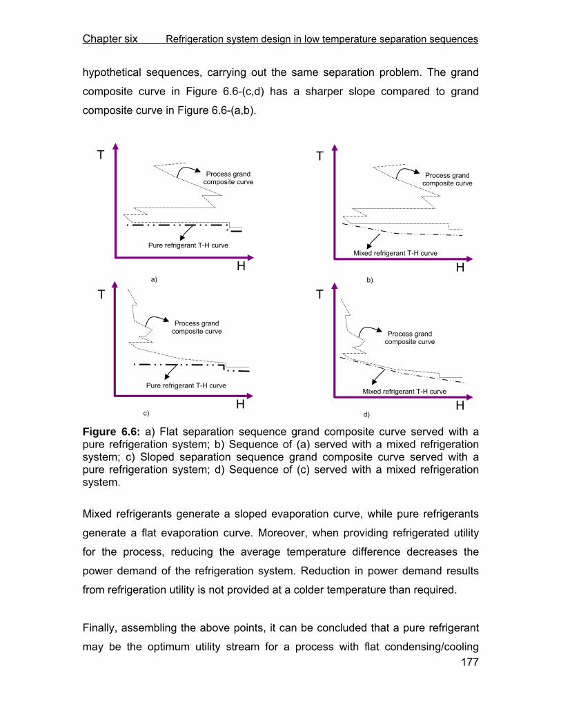
Chapter six Refrigeration system design in low temperature separation sequences
177
hypothetical sequences, carrying out the same separation problem. The grand
composite curve in Figure 6.6-(c,d) has a sharper slope compared to grand
composite curve in Figure 6.6-(a,b).
Figure 6.6: a) Flat separation sequence grand composite curve served with a pure refrigeration system; b) Sequence of (a) served with a mixed refrigeration system; c) Sloped separation sequence grand composite curve served with a pure refrigeration system; d) Sequence of (c) served with a mixed refrigeration system.
Mixed refrigerants generate a sloped evaporation curve, while pure refrigerants
generate a flat evaporation curve. Moreover, when providing refrigerated utility
for the process, reducing the average temperature difference decreases the
power demand of the refrigeration system. Reduction in power demand results
from refrigeration utility is not provided at a colder temperature than required.
Finally, assembling the above points, it can be concluded that a pure refrigerant
may be the optimum utility stream for a process with flat condensing/cooling
T
T
H
Process grand composite curve
Pure refrigerant T-H curve
T
H
Process grand composite curve
Mixed refrigerant T-H curve
H
Process grand composite curve
Pure refrigerant T-H curve
a)
c)
T
H Mixed refrigerant T-H curve
Process grand composite curve
b)
d)

Chapter six Refrigeration system design in low temperature separation sequences
178
curve; while, a mixed refrigerant refrigeration system may utilise less energy for
servicing a sloped cooling/condensing curve compared to a pure system. When
screening and optimising the separation processes, all types of separation
sequences are generated and evaluated. Therefore, both pure and mixed
refrigerants should be assumed available to the separation sequences. As a
result, the possible optimum utility will be available for each separation sequence
and it will be possible to choose the optimum refrigeration system for each
separation sequence. Therefore, a more energy efficient separation sequence
should not be rejected relative to a poor separation sequence, due to its non-
optimum utility system.
6.5 Simultaneous design of the separation and refrigeration systems A simultaneous design approach should synthesise and optimise different
variables of the process at the same time. There are a number of reasons, which
make simultaneous design of separation and refrigeration systems a better
design approach.
1. The cost (both operating and capital) of a low-temperature separation
sequence will include the costs of separation system and the costs
associated with the refrigeration system. Now, if the low-temperature
separation sequences are screened based on their cost, the costs of both
parts of the system should be optimised. In other words, the refrigeration
system should also be optimised. Otherwise, a promising separation
sequence may not survive the screening procedure because of a poor
refrigeration system. Therefore, both separation and refrigeration systems
should be optimised at the same time, in order to have confidence in the
accuracy of the cost of the process.
2. Another reason for simultaneous design of separation and refrigeration
systems is to consider the complex interactions between the two

Chapter six Refrigeration system design in low temperature separation sequences
179
processes. Operating a distillation column at a higher pressure results in a
higher condenser temperature and, hence, cheaper refrigeration will be
required. However, the relative volatility of components in some
separation tasks decreases as the pressure rises, and hence the
separation becomes more difficult at the higher pressures. More difficult
separation leads to higher loads in the condenser and reboiler. Therefore,
there is a trade-off between operating the separation device at high
pressure and employing a more expensive refrigeration system. Capturing
the trade-offs and heat integration opportunities results in a more efficient
separation sequence.
3. Moreover, it is beneficial to heat integrate the closed-loop heat-pump
refrigeration system with the separation process. A separation sequence
can create heat sinks at sub-ambient temperatures. If the refrigeration
cycle rejects the heat to these sub-ambient heat sinks rather than ambient
utility, it consumes less power. Separation sequence parameters can be
optimised so that opportunities for integrating the refrigeration system with
the separation sequence are created and explored. The following example
demonstrates this scenario.
Illustrative example Figure 6.7 shows a sequence for separation of a gas mixture in an ethylene
plant. The problem specifications are shown in Table 6.1. Shah (1999) optimised
the separation of five products in simple distillation columns without allowing heat
integration between the separation and refrigeration system. The refrigeration
system rejects the heat to the cooling water. The chosen refrigerants are
ethylene and propylene, and cooling water return temperature is set at 40˚C.
Table 6.2 shows the operating parameters and duties of each condenser and
reboiler. The total power consumption calculated for the refrigeration system of
this sequence is 38.9MW.

Chapter six Refrigeration system design in low temperature separation sequences
180
Table 6.1: problem specification for the illustrative example i Component Fraction Product Product specification
1 Hydrogen
2 Methane 0.35 A 99% recovery of methane
3 Ethylene 0.40 B 99% purity ethylene
4 Ethane 0.07 C 99% recovery of ethane
5 Propylene 0.11
6 Propane 0.01 D 98% recovery of propylene
7 i-Butadiene 0.03
8 n-Butane 0.03 E 99% recovery of i-Butadiene
Feed flowrate 5700 kmol/h, saturated vapour at 8 bar
Figure 6.7: The best simple sequence for problem of Table 6.1 in Shah (1999)
Table 6.2: Operating condition for the sequence of Figure 6.7 Condenser Reboiler
Separation P (bar)Feed
quality T (˚C)Duty
(MW)T(˚C)
Duty
(MW)
1 A/BCDE 24 1 -102 8.06 -5 13.9
2 B/CDE 16 1 -38 28.3 23 39.4
3 C/DE 27 1 5 6.5 80 8.3
4 D/E 13 1 30 6.7 86 8.1
1
2
3
C1
R1
C2
R2
C3
R3
4
C4
R4
A
B
C
D
E

Chapter six Refrigeration system design in low temperature separation sequences
181
If the separation sequence is fixed and the following heuristic rules of Wang and
Smith (2005) are applied to the refrigeration system for this sequence, the power
consumption of the refrigeration system reduces to 26.5 MW. These heuristic
rules aim at heat integrating the refrigeration system with the separation
sequence:
1. When servicing the sources and the sinks in the process, it should be
preferred to transfer the heat from sources to sinks with minimum
temperature differences first.
2. Refrigeration should be allocated to heat sources at lower temperature
prior to allocating it to those at higher temperatures.
Table 6.2 shows that there are heat sinks in the process at temperatures below-
ambient. Hence, according to rule one, these process sinks should be used for
rejecting the heat from refrigeration system before employing ambient utility.
Employing this rule, a 32% reduction in power demand for this fixed sequence
(with the set operating conditions) can be achieved. Figure 6.8 shows the reboiler
and condensers that are heat integrated through the refrigeration system. This
example shows that significant energy saving can be achieved when the
refrigeration system and separation process are integrated.
Figure 6.8: Heat integrated separation sequence and refrigeration system of Figure 6.7
1
2
3
4
Heat pumped from condenser to reboiler by
refrigeration cycles
Direct heat exchange between condenser and reboiler
Direct heat exchange between process stream and external utility
Heat pumped from condenser to external utility
A
B
C
D
E
Chapter six Refrigeration system design in low temperature separation sequences
182
4. In addition, there is another incentive to simultaneously consider heat
integration options in the separation and refrigeration systems. In a
sequential approach, the separation process is heat integrated first. Then
the remaining process streams (that are not heat integrated within the
separation sequence) are allowed to integrate with the refrigeration
system (Wu and Zhu, 2002). A simultaneous approach can generate more
cost-effective designs compared with a sequential approach, as it can
capture the interactions between different parts of the process. Example 1
in Chapter 3 illustrates the effect of simultaneously accounting for heat
integration in the separation sequence and the refrigeration system. The
example shows that heat integrating a separation heat sink with the
condenser of the refrigeration system can be more energy efficient than
integrating it with a heat source in the sequence. Such integration
opportunities can only be identified if heat integration, within the
separation sequence and between the separation and refrigeration
systems, is not considered sequentially. In other words, if the separation
sequence is heat integrated and the remaining streams are allowed to
integrate with the refrigeration system, then some more effective heat
integration opportunities between separation and refrigeration processes
may be missed.
5. Opportunities for employing internal refrigeration sources can be explored.
Process operating conditions (such as pressure) can be adjusted to allow
for heat integration of process streams. Heat integrating the sub-ambient
sources and sinks in the process will reduce the need for external and
expensive refrigeration system. The result will be a lower operating and
investment cost.
The refrigeration system provides the required utility for the process at sub-
ambient temperatures and interacts with the process through the heat exchanger
network (HEN). Therefore, in this work, in order to simultaneously design and
Chapter six Refrigeration system design in low temperature separation sequences
183
optimise the separation and refrigeration systems, the two processes are linked
through the heat exchanger network. The details for heat exchanger network
design problem are presented in Chapter 3. A short review of the HEN design
methodology will be presented in Section 6.6.1, where the links between the
refrigeration and separation systems in HEN system are introduced.
6.6 HEN design methodology for low-temperature separation processes 6.6.1 A review of HEN design methodology for processes at above-ambient temperature The general optimisation framework in this work for the synthesis and
optimisation of a heat integrated separation sequence was presented in Chapter
5. For generating each trial solution, the optimiser suggests a separation
sequence. A heat exchanger network should then be designed for the fixed
sequence. The HEN should consider heat integration opportunities between
different streams in the process.
A cost matrix (Figure 3.8) is calculated that determines the utility cost for each
match between all the process sources and sinks. In an above ambient system,
the cost of each match is either equal to the cost of utility (if the process stream
is matched with a utility) or negligible (if the process stream is directly heat
integrated with another process stream). Heat pumping between sources and
sinks at above-ambient temperature is not allowed. Therefore, for penalising
such matches between a heat source and a heat sink (at above ambient), where
the source is colder than the sink, the Carnot model with a low efficiency is used
for an imaginary heat pump (Equation 3.15). The imaginary heat pump will be
working between the fixed temperatures of the heat source and the heat sink
after applying the appropriate minimum temperature approaches and hence, a
fixed cost can be determined for the heat-pumped match. Therefore, the
operating cost, per unit load of heat transferred in each match, can be calculated
and the cost matrix for the HEN problem can be fixed.

Chapter six Refrigeration system design in low temperature separation sequences
184
Thereafter, the objective function for minimising the operating cost of the HEN
(and hence the separation sequence) can be formulated as a linear programming
optimisation problem (LP) for an above ambient process. The only variables are
the heat loads on each match. In other words, the amount of heat transferred
between each process source and process sink is optimised. The energy
balances for the source and sink streams form the constraints of this problem.
6.6.2 Modification of HEN design methodology for application in low-temperature processes In a below-ambient process, heat pumps or refrigeration cycles are utilised as
utilities for servicing heat sources at sub-ambient temperatures. The refrigeration
system absorbs heat from the sub-ambient sources and rejects it to the available
sinks at higher temperatures than the source. In Section 6.6.1, it was mentioned
that in the HEN employed design method in this work, the heat transfer from a
colder source to a hotter sink is forbidden at above ambient temperatures. Such
matches are penalised using the Carnot model with a very low efficiency.
However, in a below-ambient process, it is essential to find the true costs of the
refrigeration system that operates between a source and a sink, where the
source is colder than the sink. Therefore, the incentive is to develop a method for
evaluating the cost of the refrigeration system that transfers heat in the matches
between the sources and sinks.
It is desired to use the energy cost of the refrigeration cycles in the cost matrix of
the HEN model introduced in Chapter 3. The HEN model identifies the heat
transfer possibilities between the streams in the separation system and available
utility to the process, such as cooling water and steam. If the refrigeration system
required for servicing the sub-ambient streams has its cost included in the HEN
design model, the separation system and the refrigeration system are linked
through the heat exchanger network. Hence, the energy cost of the overall
system, i.e. the separation process and the refrigeration system, can be

Chapter six Refrigeration system design in low temperature separation sequences
185
estimated simultaneously. The challenge now is to create a robust methodology
for evaluating and costing the performance of the refrigeration system.
Many different types and structures of refrigeration systems can absorb heat
from a specific source. Even if the refrigeration evaporation and condensation
temperatures are fixed, there are still many degrees of freedom, such as the type
of refrigerant, and the number of cascades. Therefore, the cost of transferring
heat from a source to a sink stream, which is served by a heat pump, will not be
unique and it can be optimised. In a below-ambient system, the refrigeration
system is the main utility and its cost affects the ranking of the separation
sequences. Consequently, in order to accurately judge (and evaluate) the cost of
a sequence, which includes the cost of its refrigeration system, its refrigeration
system should be optimised, as discussed in Section 6.5.
In this work, a rigorous approach has been presented, which uses equations of
states and energy balances to calculate the power demand of the compressors in
the refrigeration system.
6.7 Synthesis and evaluation of the refrigeration system 6.7.1 The pursued incentives for the refrigeration system model The problem of optimising the heat integrated separation sequence is a complex
combinatorial problem. There are numerous options and degrees of freedom in
separation sequence design. Moreover, the refrigeration system design problem
alone is also a highly non-linear and non-convex problem (Del Nogal, 2006).
Simultaneously optimising the separation and refrigeration systems is a
challenging task as it involves solving large and nonlinear problems
simultaneously.
To develop a methodology for simultaneous design and optimisation of
separation and refrigeration system, one challenge is to adopt an appropriate
approach for evaluating the refrigeration system performance. Firstly, it is
Chapter six Refrigeration system design in low temperature separation sequences
186
attractive that the refrigeration model encompasses various refrigeration
provision strategies and provides information regarding the optimal refrigeration
strategy. These strategies may include the choice of refrigerant type (i.e. pure or
mixed) or the structure of the refrigeration system (e.g. number of cascades).
Secondly, the model should be able to capture opportunities for heat integration
with the rest of the process and enable simultaneous design of separation and
refrigeration systems. Thirdly, the complexity of the designed refrigeration
processes should be controlled. A process may be highly energy-efficient, but not
practically economic due to its high capital and maintenance costs and its
operational difficulties. In a refrigeration system that uses rotating equipment, it is
essential to avoid complex designs that are expensive to build and difficult to
operate.
Another key factor, to ensure the robustness of the approach, is the amount of
detail included in the model. The model should be simple enough to be solved
within a reasonable computational time. However, the simplicity of the model
should not be at the expense of the accuracy and practicality of the design
solutions generated.
6.7.2 Superstructure and assumptions for the refrigeration system model The superstructure for the refrigeration system is presented in Figure 6.9. This
superstructure contains various structural options. Cascaded systems with
multistage cycles can be generated by this superstructure. Multiple refrigeration
and rejection levels are allowed to create heat integration opportunities with the
background process. The superstructure includes multistage cycles with each
stage at a different pressure. Both pure and mixed refrigeration systems are
considered. Cycles with constant refrigerant composition in different stages of the
compressor can be obtained from this superstructure.
The proposed superstructure does not support multi-stage mixed refrigeration
systems with a single pressure level (Del Nogal, 2006). Considering such mixed
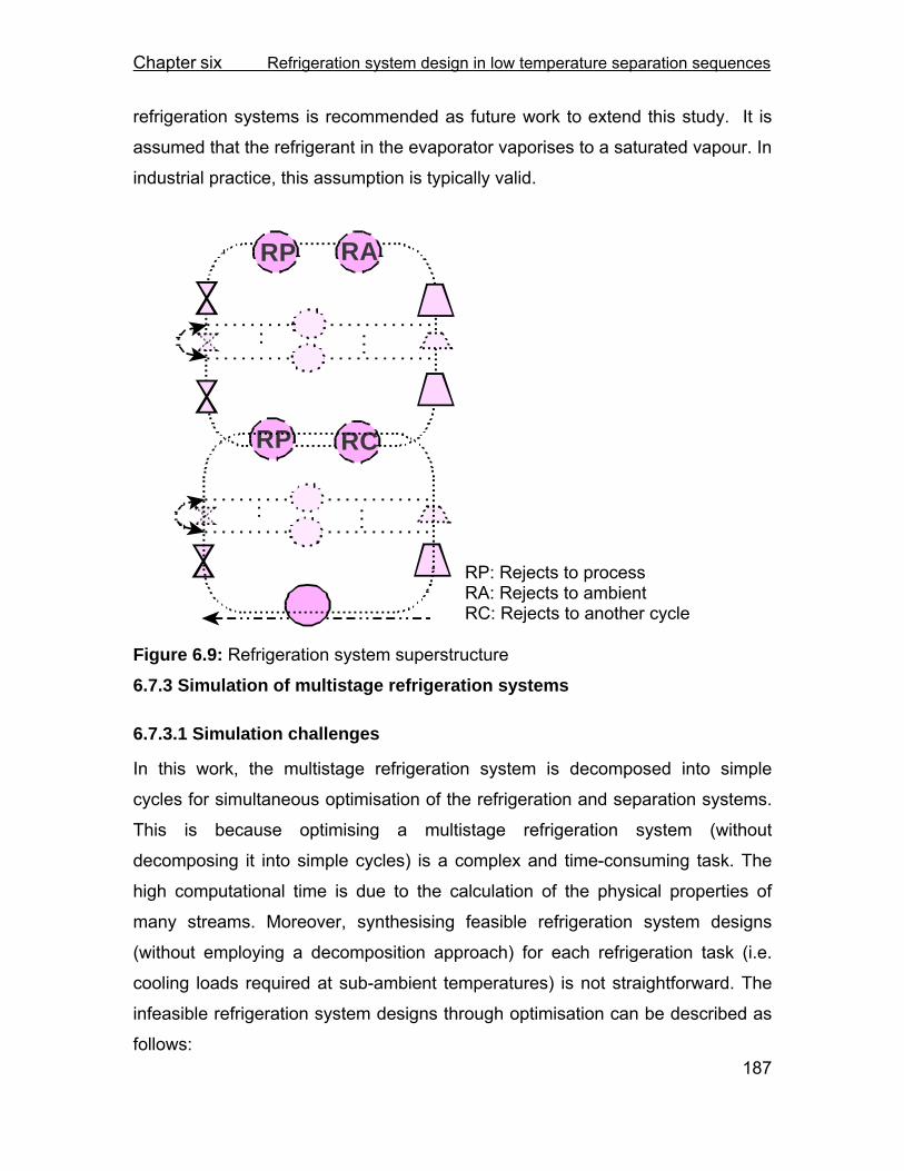
Chapter six Refrigeration system design in low temperature separation sequences
187
refrigeration systems is recommended as future work to extend this study. It is
assumed that the refrigerant in the evaporator vaporises to a saturated vapour. In
industrial practice, this assumption is typically valid.
Figure 6.9: Refrigeration system superstructure
6.7.3 Simulation of multistage refrigeration systems
6.7.3.1 Simulation challenges
In this work, the multistage refrigeration system is decomposed into simple
cycles for simultaneous optimisation of the refrigeration and separation systems.
This is because optimising a multistage refrigeration system (without
decomposing it into simple cycles) is a complex and time-consuming task. The
high computational time is due to the calculation of the physical properties of
many streams. Moreover, synthesising feasible refrigeration system designs
(without employing a decomposition approach) for each refrigeration task (i.e.
cooling loads required at sub-ambient temperatures) is not straightforward. The
infeasible refrigeration system designs through optimisation can be described as
follows:
RARP
RP RC
RP: Rejects to process RA: Rejects to ambient RC: Rejects to another cycle

Chapter six Refrigeration system design in low temperature separation sequences
188
The scenario is that the refrigeration system is given the task of providing sub-
ambient cooling to the process. A multistage cycle, which can have a mixture as
the refrigerant, should provide this refrigeration duty at the required
temperatures. The first design step of the refrigeration system is to choose the
composition for the refrigerant fluid that, when expanded in the refrigeration
cycle, would be cold enough for the required refrigeration task. When the
composition of the refrigerant in the cycle is optimised, there is always the
chance that the composition proposed by the optimisation framework is not
capable of providing the refrigerated utility as cold as is required. Therefore,
many infeasible systems occur in the optimisation process.
In addition, finding the correct pressure drop in the cycle to have the refrigerant
at the required temperature demands a trial and error procedure. Mixed
refrigerants evaporate over a temperature range and there is not a unique
pressure level for a specific refrigeration temperature, even when using a specific
mixture of refrigerants. In other words, there is no simple and direct relation
between the temperature and pressure for a mixture. The complexity will be even
higher if the composition of the refrigerant changes in different levels of the cycle.
Another possible approach is that, instead of determining the pressure levels for
each refrigeration temperature required by the process, first a structure and set
of pressure levels of the multistage cycle are proposed and set by the
optimisation tool. This pre-determined refrigeration system would be responsible
to service the refrigeration duty required by the process. In this scenario, also
there is no guarantee that the composition and/or refrigeration pressure levels
proposed by the optimiser can generate a feasible refrigeration system for
servicing the cooling demand in the process at the required temperatures.
Therefore, similar to the first scenario discussed above, many infeasible solutions
occur throughout the optimisation.
Chapter six Refrigeration system design in low temperature separation sequences
189
To summarise, according to the experience gained in this work, optimising
complex refrigeration structures is possible (Del Nogal, 2006; Vaidyaraman, 1999
and 2002). However, the procedure is rather tedious and time consuming due to
many different options and also infeasible solutions. Therefore, it will not be a
robust approach for optimising the refrigeration system in the context of
separation sequence design problem, since the computational time will be high.
6.7.3.2 Decomposition approach
To overcome the problems mentioned in Section 6.7.3.1, the approach employed
in this work merges simple cycles to construct the multistage refrigeration
system. Figure 6.10-(b) illustrates the two cycles that are used to evaluate the
power demand and temperature in the multi-stage cycle, shown in Figure 6.10-
(a). The approach is based on approximating the performance of a multistage
refrigeration cycle by decomposing it to a number of simple cycles. The reverse
action (i.e. merging of simple cycles) can be adopted for simulating and
evaluating the performance of a multistage refrigeration cycle. However, before
further elaborating on how the approach is applied, it needs to be verified.
The proposed decomposition approach is an approximation approach. Some
amount of error will be expected. The error is caused by the mixing effects at the
inlet to the compressor in the case of a cycle with multiple refrigeration levels or
the inlet to the expander for a multi-rejection level cycle. However, through the
following two examples, it will be shown that the amount of error is acceptable for
the multi-stage configurations that are used in this work. The examples will
provide evidence using a mixed refrigerant. The compressor efficiencies and
pressures of the corresponding stages in the multistage cycle and its
decomposed simple cycles are specified the same. The inlet and outlet
temperatures of the evaporator are the refrigeration temperatures, which are
provided for the process. The condenser outlet temperature is also considered as
the rejection level in the cycle.

Chapter six Refrigeration system design in low temperature separation sequences
190
The main parameters of the cycles, which represent a multi-stage cycle, are:
• the evaporation and condensation temperatures in the cycle (that
determines at which temperature the cycle absorbs and rejects heat) and,
• the power demand per unit load of heat at each temperature level (which
determines the operating cost of the system).
In the following illustrative examples, the above parameters are compared
between a multistage cycle and the associated decomposed simple cycles. The
calculations were carried out in HYSYS.
Illustrative example i. Decomposing a complex cycle with multiple refrigeration levels This example aims at determining the amount of error that is associated with
decomposing a complex cycle with multi-refrigeration levels into simple cycles.
The multistage cycle has a single rejection level. Figure 6.10 shows the
multistage cycle, together with its simple cycle representation. Table 6.3
summarises the operating conditions for the cycles in Figure 6.10. The power
demand is per unit of cooling duty provided by the cycle at each refrigeration
level.
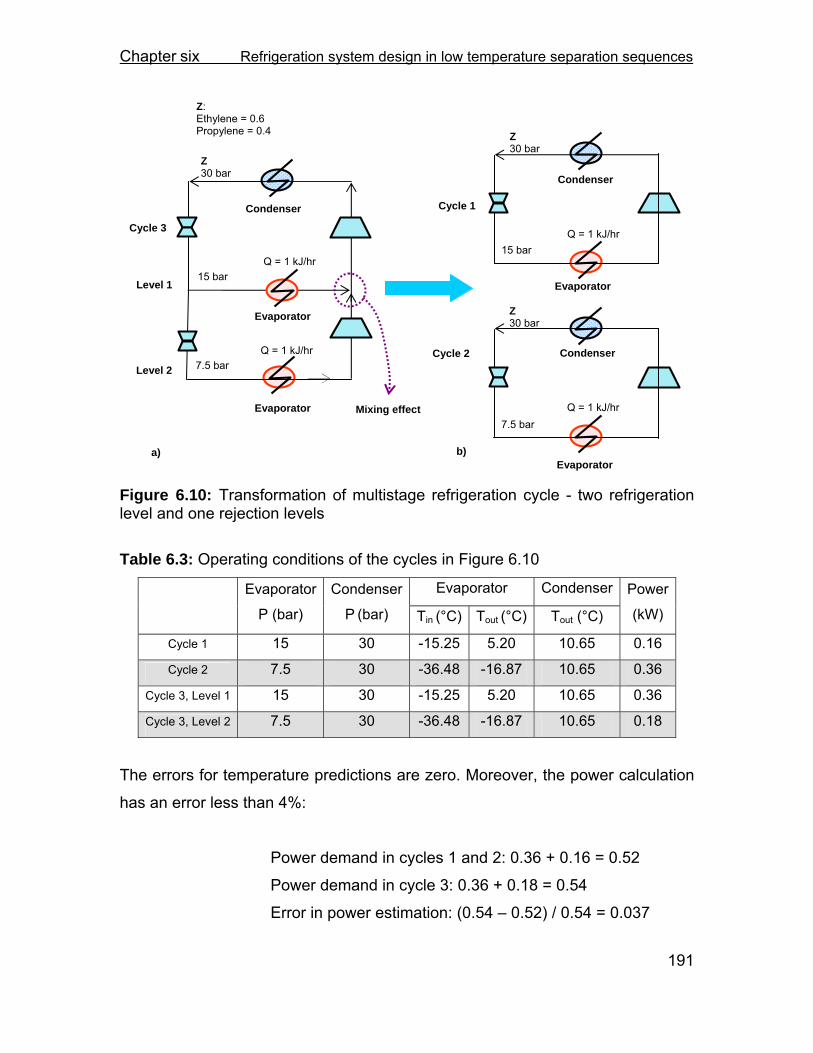
Chapter six Refrigeration system design in low temperature separation sequences
191
Figure 6.10: Transformation of multistage refrigeration cycle - two refrigeration level and one rejection levels
Table 6.3: Operating conditions of the cycles in Figure 6.10
Evaporator Condenser
Evaporator
P (bar)
Condenser
P (bar) Tin (°C) Tout (°C) Tout (°C)
Power
(kW)
Cycle 1 15 30 -15.25 5.20 10.65 0.16
Cycle 2 7.5 30 -36.48 -16.87 10.65 0.36
Cycle 3, Level 1 15 30 -15.25 5.20 10.65 0.36
Cycle 3, Level 2 7.5 30 -36.48 -16.87 10.65 0.18
The errors for temperature predictions are zero. Moreover, the power calculation
has an error less than 4%:
Power demand in cycles 1 and 2: 0.36 + 0.16 = 0.52
Power demand in cycle 3: 0.36 + 0.18 = 0.54
Error in power estimation: (0.54 – 0.52) / 0.54 = 0.037
Cycle 3
Z: Ethylene = 0.6 Propylene = 0.4
Z 30 bar
Q = 1 kJ/hr
Z 30 bar
15 bar
Q = 1 kJ/hr 7.5 bar
Level 1
Level 2
Evaporator
Evaporator
Condenser
Q = 1 kJ/hr
Z 30 bar
15 bar
Cycle 1
Evaporator
Condenser
Q = 1 kJ/hr 7.5 bar
Cycle 2
Evaporator
Condenser
a) b)
Mixing effect
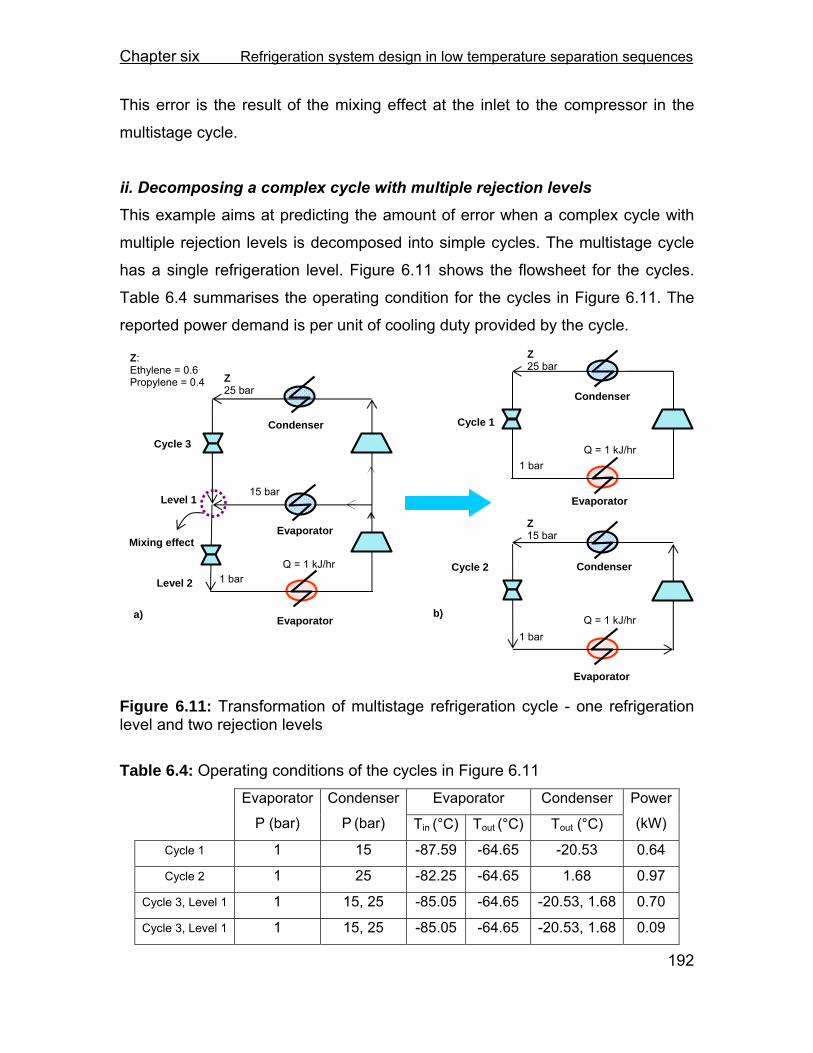
Chapter six Refrigeration system design in low temperature separation sequences
192
This error is the result of the mixing effect at the inlet to the compressor in the
multistage cycle.
ii. Decomposing a complex cycle with multiple rejection levels
This example aims at predicting the amount of error when a complex cycle with
multiple rejection levels is decomposed into simple cycles. The multistage cycle
has a single refrigeration level. Figure 6.11 shows the flowsheet for the cycles.
Table 6.4 summarises the operating condition for the cycles in Figure 6.11. The
reported power demand is per unit of cooling duty provided by the cycle.
Figure 6.11: Transformation of multistage refrigeration cycle - one refrigeration level and two rejection levels
Table 6.4: Operating conditions of the cycles in Figure 6.11 Evaporator Condenser
Evaporator
P (bar)
Condenser
P (bar) Tin (°C) Tout (°C) Tout (°C)
Power
(kW)
Cycle 1 1 15 -87.59 -64.65 -20.53 0.64
Cycle 2 1 25 -82.25 -64.65 1.68 0.97
Cycle 3, Level 1 1 15, 25 -85.05 -64.65 -20.53, 1.68 0.70
Cycle 3, Level 1 1 15, 25 -85.05 -64.65 -20.53, 1.68 0.09
Z 25 bar
Z 15 bar
Z: Ethylene = 0.6 Propylene = 0.4 Z
25 bar
15 bar
Q = 1 kJ/hr 1 bar
Cycle 3
Level 1
Level 2
Evaporator
Evaporator
Condenser
Q = 1 kJ/hr 1 bar
Cycle 1
Evaporator
Condenser
Q = 1 kJ/hr 1 bar
Cycle 2
Evaporator
Condenser
a) b)
Mixing effect

Chapter six Refrigeration system design in low temperature separation sequences
193
The results in Table 6.4 show some error in the inlet temperature to the
evaporator of the refrigeration system. Cycle 1 is under-predicting the
refrigeration temperature at level 1 of Cycle 3 by 2.5 °C and Cycle 2 is over-
predicting this temperature by 2.8 °C. Obviously, this is a very small error (~3%).
This error is due to the mixing effects at the inlet to the throttle valve in the
multistage cycle. In terms of power demand, the error is almost 3%. It should be
highlighted that in order to compare power demand per unit load of refrigeration
in this case, the sum of the reported values in the Table 6.4 should be divided by
2. In other words, power demand per unit load of refrigeration duty provided by
simple cycles equals:
(0.64 + 0.97) / 2 = 0.81
Otherwise the power demand for two unit loads of cooling duty will be calculated.
The examples demonstrate that even though there is some error associated with
decomposition approach, the size of the error is acceptable for the screening
purposes in this work, even for mixed refrigeration systems.
6.7.3.3 Evaluation of cascaded refrigeration cycles using decomposition approach
A cascade of multistage refrigeration cycles can also be presented as cascades
of simple cycles. Figure 6.12-(a) shows a multistage cycle that is cascaded
against a simple cycle. Figure 6.12-(b) illustrates the simple cycles that are
representing the cascading of the lower cycle against the upper cycle. Reversely,
the simple cycles of Figure 6.12-(b) can be merged to form the lower multistage
cycle that is cascaded against the top cycle. If the heat pump system should
accept the heat at T1 and rejects at T4, through a cascade, a refrigerant ‘A’ will
serve in the cycle operating between T1 and T3 and another refrigerant ‘B’ will
operate between T3 and T4. This system can be simulated, as shown in Figure

Chapter six Refrigeration system design in low temperature separation sequences
194
6.12, using simple cycles. Cycles I and II, which have the same refrigerant fluid,
are merged to form the multistage Cycle III.
Figure 6.12: Transformation of cascades of multistage refrigeration cycle
The partition temperature is the temperature at which the upper cycle in the
cascade absorbs heat from a lower cycle. The partition temperature for two
cascaded simple cycles in Figure 6.12 is shown. Partition temperature is one of
the parameters that should be optimised, when cascading a number of (multi- or
single-stage) cycles. By optimising the partition temperature, the type of the
refrigerant which is employed at each temperature is optimised.
If the compositions of the two cycles are known, the upper and lower limits for the
partition temperature, partT , are:
MAXCYC_LOWpart
MINCYC_UP TTT ≤≤ 6.1
where MINCYC_UPT is the smallest temperature that the upper cycle can operate at
and is the normal boiling point for the refrigerant of the upper cycle. MAXCYC_LOWT is
the maximum temperature that the lower cycle can reject the heat at.
T1
T2
T3
T4
T1
T3
T4
T2
T3
T4
Refrigerant A
Refrigerant A
Refrigerant A
Refrigerant B
Refrigerant B Refrigerant B
a)
b)
(I)
(II)
(III)
:Tpart Partition temperature
Tpart

Chapter six Refrigeration system design in low temperature separation sequences
195
6.7.3.4 Summary
Sections 6.7.3.2 and 6.7.3.3 describe how by assessing simple cycles, cascades
of multistage cycles can be evaluated. This approach provides a tool for
designing the refrigeration system. For a given refrigeration task in the process,
the elements (i.e. simple cycles) of the refrigeration system are selected, such
that the utility demand of the corresponding source and sink streams in the
process are serviced. Thereafter, simple cycles with the same refrigerant
composition can be merged to form a multistage refrigeration cycle.
6.7.4 Refrigeration system database In Section 6.7.3.1, the reasons for assuming a decomposed multistage cycle,
while carrying out simultaneous optimisation of the refrigeration and separation
systems, was discussed.
In this work, numerical experiments were carried out in which the separation and
refrigeration systems were optimised simultaneously, using the decomposition
approach for the design of refrigeration systems. For each match between the
source and the sink for which a heat pump is required, a simple cycle or a
cascade of simple cycles that absorbs heat from the source and rejects the heat
to the sink are simulated. Briefly, the compositions of the refrigerants and the
partition temperature for cascaded systems are proposed by the optimiser. Then
the algorithm for design of the refrigeration system determines the pressure
levels of the simple cycles, so that the cycles operate between the source and
sink temperatures. However, there is no guarantee that the proposed
compositions can absorb heat from the source at the required temperature and
reject heat at the sink temperature. Therefore, many time-consuming trial
solutions will happen, which increases the computational time significantly.
A further assessment of the approach revealed that many time consuming
calculations (such as calculating the physical properties of the streams) in the
refrigeration system were repeated unnecessarily. Let us briefly review the

Chapter six Refrigeration system design in low temperature separation sequences
196
optimisation framework to clarify this issue. At each trial solution of the
optimisation, a separation sequence is proposed by the optimiser. Then the heat
exchanger network and also the refrigeration system for the proposed separation
sequence are designed and optimised. In the next trial solution of the
optimisation, one parameter in the process may be altered. For instance, the
change may be a small modification in the feed quality. This change may not
require the refrigeration design to be altered significantly and since the
refrigeration system optimisation parameters are not changed, most parts of the
refrigeration system remain similar to the previous trial solution. However, all the
time consuming calculations of the refrigeration system are repeated.
In order to overcome the unnecessary repetitive calculations and also to find the
feasible solutions more quickly, the following strategy is proposed:
Before the start of optimisation, a database of simple refrigeration cycles,
that can be built using the available refrigerants and within their operating
pressure ranges, are simulated and their operating conditions and power
demand are stored in a database. Throughout the optimisation, rather
than simulating each proposed simple cycle, a search in the database is
performed in order to find feasible cycle(s).
6.7.4.1 Building the simple cycle database
i. Composition set In order to build the database of simple cycles, various compositions of available
refrigerants are generated and stored. The refrigeration cycle database will
include cycles with both pure and mixed refrigerants. The approach allows the
user to determine the size of the composition intervals, as shown in Figure 6.13.
The smaller the intervals, the more refrigerant compositions can be examined in
the optimisation and the composition of the refrigerant can be optimised in finer

Chapter six Refrigeration system design in low temperature separation sequences
197
detail. A uniform composition interval is chosen for compositions in this work in
order to generate the refrigerant composition set, X.
{ }ionst compositrefrigerannumber of ,1:i|Xi=X
The following illustrative example shows the composition grid with an interval
size of 0.1.
Illustrative example Methane, ethylene and propylene are assumed as available refrigerants. Figure
6.13 shows the composition grid for these refrigerants with an interval size of 0.1.
Two example compositions are shown on the diagram.
0 1
1
Figure 6.13: Composition grid for mixtures of M, E and P
(M: Methane, E: Ethylene, P: Propylene)
ii. Pressure sets
After the set of refrigerant compositions is developed, different possible
refrigeration and rejection pressures for simple cycles with the refrigerant
composition of iX are generated. First, for each composition the lower, LBxi
P , and
the upper, UBxi
P , pressure bounds of the simple cycles, which use this refrigerant
(M: 0.2, E: 0.5, P: 0.3)
(M: 0.4, E: 0.2, P: 0.4)
M
E
Mole fraction
of ethylene
Mole fraction
of methane
P

Chapter six Refrigeration system design in low temperature separation sequences
198
are set. LBxi
P is the minimum pressure of the refrigeration level in the simple cycle
and is chosen to be equal to the atmospheric pressure. UBxi
P is the maximum
pressure of the rejection level in the simple cycle with the refrigerant composition
iX . UBxi
P is the bubble pressure of the refrigerant with the composition iX at
which the latent heat of the refrigerant is 35% of the latent heat of the refrigerant
at atmospheric pressure. The UBxi
P is determined by trial and error using
equations of state and is selected to avoid critical conditions and poor refrigerant
latent heat.
In order to generate different refrigeration cycles (that operate between different
pressure levels), the interval between LBxi
P and UBxi
P is discretised according to a
step size ( PΔ ). PΔ is set by the user. The number of the pressure segments, SegmentsnP , is given by:
⎟⎟⎠
⎞⎜⎜⎝
⎛ −=
P)PP(
INTnPLB
xUBxSegments ii
Δ 6.2
INT stands for the function that returns the integer of a real number. The
partitioned pressures form the sets of pressures of the lower ( LL,jxi
P ) and upper
( UL,kxi
P ) levels in the simple cycles of each refrigerant with the composition iX .
{ }
{ }SegmentsUBx
LBx
LBx
UL,kx
SegmentsSegmentsLBx
LBx
LBx
LBx
LL,jx
nP,1:k|P,...,P2P,PPP
nP,1:j|P)1nP(P,...,P2P,PP,PP
iiii
iiiii
ΔΔ
ΔΔΔ
++=
⋅−+++=
The values for the pressures in the LL,jxi
P and UL,kxi
P sets are then paired, so that
one would be the pressure of the lower level, LL,jxi
P , and the other the pressure of
the upper level, UL,kxi
P , in a simple cycle. In other words, every feasible

Chapter six Refrigeration system design in low temperature separation sequences
199
combination of the elements in LL,jxi
P and UL,kxi
P sets for the composition iX is used
to form the pressures set for the simple cycles, k,jP , of the database. A pressure
pair is feasible if the pressure of the upper level is higher than the lower level
pressure.
{ }k)|j,P(PP ULk,x
LL,jxk,j ii
≤=
iii. Simulation of simple cycles
Each member of the set of pairs of pressure, k,jP , together with its associated
refrigerant composition, iX , represents a simple refrigeration cycle, ( )kj,
i
PXCyc , as
shown in the Figure 6.14.
)P,P,X(Cyc ULk,x
LLj,xi
PX ii
kj,
i=
The next step in building the refrigeration system database is to calculate the
temperatures in the cycle and the power demand per unit load of cooling. The
physical property calculations are performed using Peng Robinson equation of
state.
It is assumed that the superheated refrigerant vapour from the outlet of the
compressor is condensed to a saturated liquid at a constant pressure, ULk,xi
P . The
saturated liquid is then let down to LLj,xi
P in a throttle valve. The low pressure fluid,
LLj,xi
P , is then vaporised to a saturated vapour in the evaporator.
The first parameter to be calculated is the bubble temperature of the refrigerant
fluid, jkxi
Tcnd , at the rejection pressure, ULk,xi
P .
An isenthalpic throttle valve is assumed to perform the pressure drop in the
cycle. The enthalpy at the exit of the valve will be equal to the enthalpy at the exit
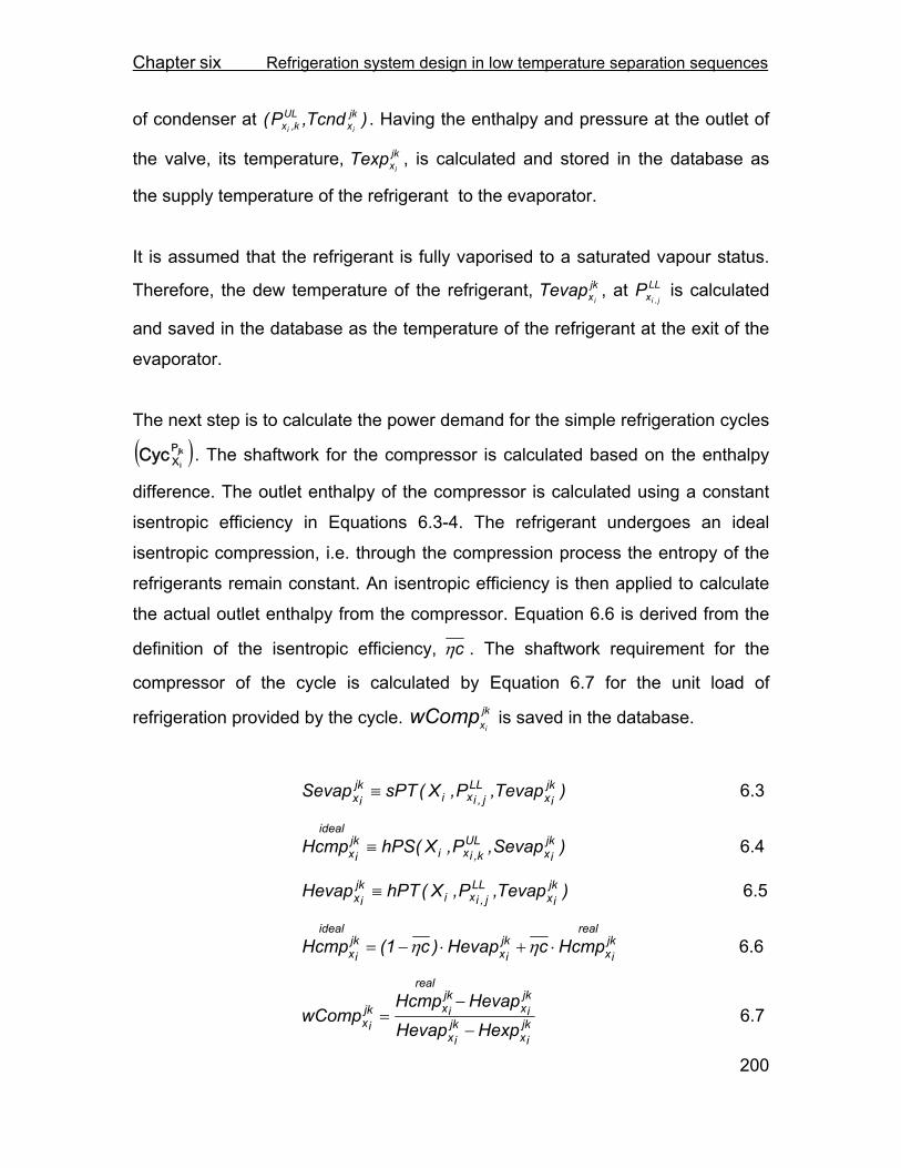
Chapter six Refrigeration system design in low temperature separation sequences
200
of condenser at )Tcnd,P( jkx
ULk,x ii
. Having the enthalpy and pressure at the outlet of
the valve, its temperature, jkxi
expT , is calculated and stored in the database as
the supply temperature of the refrigerant to the evaporator.
It is assumed that the refrigerant is fully vaporised to a saturated vapour status.
Therefore, the dew temperature of the refrigerant, jkxi
Tevap , at LLx j,i
P is calculated
and saved in the database as the temperature of the refrigerant at the exit of the
evaporator.
The next step is to calculate the power demand for the simple refrigeration cycles
( )jk
i
PXCyc . The shaftwork for the compressor is calculated based on the enthalpy
difference. The outlet enthalpy of the compressor is calculated using a constant
isentropic efficiency in Equations 6.3-4. The refrigerant undergoes an ideal
isentropic compression, i.e. through the compression process the entropy of the
refrigerants remain constant. An isentropic efficiency is then applied to calculate
the actual outlet enthalpy from the compressor. Equation 6.6 is derived from the
definition of the isentropic efficiency, cη . The shaftwork requirement for the
compressor of the cycle is calculated by Equation 6.7 for the unit load of
refrigeration provided by the cycle. jkxi
wComp is saved in the database.
)Tevap,P,X(sPTSevap jkix
LLj,ixi
jkix ≡ 6.3
)Sevap,P,X(hPSHcmp jkix
ULk,ixi
idealjkix ≡ 6.4
)Tevap,P,X(hPTHevap jkix
LLj,ixi
jkix ≡ 6.5
realjkix
jkix
idealjkix HcmpcHevap)c1(Hcmp ⋅+⋅−= ηη 6.6
jkix
jkix
jkix
realjkixjk
ix expHHevapHevapHcmp
wComp−
−= 6.7

Chapter six Refrigeration system design in low temperature separation sequences
201
Figure 6.14: Operating parameters of a simple refrigeration cycle
The information representing each simple cycle, jk
i
PXCyc , is stored as a function of
composition iX , refrigeration level, LLj,xi
P and rejection level ULk,xi
P for the future
reference.
)wComp,Tcnd,Tevap,expT,P,P,( jkx
jkx
jkx
jkx
ULx
LLj,x iiiik,iii
PX XCyc jk
i=
6.8 Synthesis and optimisation of refrigeration system 6.8.1 Combined HEN and refrigeration system design In order to consider the opportunities for heat integration with the rest of process,
the refrigeration system design algorithm is combined with the heat exchanger
network design algorithm. Recalling from Section 6.6, the sets of temperatures
and duties of sources and sinks of the process are presented to the heat
exchanger network design algorithm. A cost matrix is formed, in which the cost of
heat exchange between each source with each sink is calculated. If the source is
colder than the sink a heat pump system is required. For such matches, that also
have sub-ambient sources, the refrigeration system design algorithm is used for
costing the matches. The task for the refrigeration system design problem can be
summarised as follows:
jkx
ULk,x ii
Tcnd,P,iX
LLj,xi
P
jkxi
expTjkxi
Tevap
jkxi
wComp
jk
i
PXCyc

Chapter six Refrigeration system design in low temperature separation sequences
202
Identify the elements (simple cycles) of the refrigeration system that can
absorb heat from a source with supply temperature of msource,inT and target
temperature of msource,outT and reject heat to a sink with the target
temperature of nsinkout,T (Figure 6.15).
ambientsub
sourcem
source,injkx DTTTevap
i
−−≤ 6.8
ambientsubsource
msource,out
jkx DTTexpT
i
−−≤ 6.9
sinkn
sinkout,jkx DTTTcnd
i+≥ 6.10
Figure 6.15: Rules employed for ensuring heat transfer feasibility between process and refrigeration system
For each set of source and sink temperatures, the refrigeration system design
algorithm searches the refrigeration database to identify a number of simple and
cascaded cycles that can carry out the required heat transfer task. The cycles or
cascaded cycles, which perform the task with the least amount of shaftwork are
selected and allocated to the relevant source-sink match. Hence a fixed cost can
be calculated and assigned to the match in the cost matrix that uses the
corresponding refrigeration cycle. So, in Equation 3.14:
hputilitymn
powermn
totalmn CCC −+= 3.14
msource,inT
msource,outT
nsinkout,T
jkxi
Tevapjkxi
expT
jkxi
Tcnd

Chapter six Refrigeration system design in low temperature separation sequences
203
powermnC is the cost of shaftwork for the cycle (or cascade of cycles) serving the
match mn. If the sink is a utility (e.g. cooling water), the cost of the utility, hputility
mnC − , is also added to the cost of shaftwork to calculate the energy cost, totalmnC , for the match between the source m and the sink n. The cost matrix is then
used to optimise the load on each match and calculate the minimum operating
cost, which includes the cost of hot and cold utility and electricity demand of the
system.
Minimise ∑=
=
=sink
source
1,nn
1,nm
totalmnmn C*Qf(Q) 3.10
After carrying out the minimisation of the energy cost (Equation 3.10), the
refrigeration cycles for matches in the cost matrix that does not exchange heat
are excluded from the refrigeration system.
6.8.2 Optimisation parameters in the refrigeration system The key degrees of freedom for enhancing the performance of the refrigeration
system are the number, type and composition of refrigerant fluids, the number of
compression stages, inlet and outlet pressure to each compressor stage and the
cascading strategy.
Section 6.4 discusses issues regarding the choice of refrigerants and the
importance of considering both pure and mixed refrigerants in simultaneous
optimisation of refrigeration and separation systems. The composition of mixed
refrigerant is a key degree of freedom. This variable should be optimised to
minimise the average temperature lift in the refrigeration system.
The number of compression stages and the inlet and outlet pressures to each
compressor stage determine the refrigeration temperature. Figure 6.2-(c) shows
a temperature-enthalpy profile for a process and its refrigeration system with one
Chapter six Refrigeration system design in low temperature separation sequences
204
compression stage. In Figure 6.3-(c) the same process is served by a
refrigeration system with three compression stages. The refrigeration system in
Figure 6.2-(a) provides the cooling for a wide temperature range at a single
refrigeration temperature and has a poor performance (i.e. high shaftwork
demand). Obviously, the system in Figure 6.3-(c) presents a closer match
between the process temperature profile and the refrigeration system
temperature profile. This closer match indicates that cooling is provided for the
process at a temperature that is no colder than what is required and the average
temperature lift for this refrigeration system is lower. Considering that providing
refrigeration at a colder temperature demands more power, the system in Figure
6.3-(c) is likely to have a lower operating cost compared to the system in Figure
6.3-(a). However, the capital cost of the system increases as the number of
compression stages is increased. Therefore, the number of compression stages
should be controlled or the capital and operating cost trade-offs should be
optimised.
Another key degree of freedom is the structure of cascaded cycles. The
decisions, that which cycle is cascaded against which other cycle and at which
partition temperature, should be optimised. In fact optimisation of the cascaded
structures optimises the type and the operating temperature range of
refrigerants.
The following degrees of freedom in the optimisation of the refrigeration system
are considered in this work:
• Number of cascaded cycles or the number of different refrigerant fluids
• Type and composition of the each refrigerant or type of the refrigerant
• Number of refrigeration (absorption/evaporation) levels in each cycle
• Number of rejection (condensation) levels in each cycle
• Pressure and therefore the temperature at each level
• Cascading strategy (i.e. which cycle is cascaded against which cycle.)
• Partition temperature in the cascaded systems
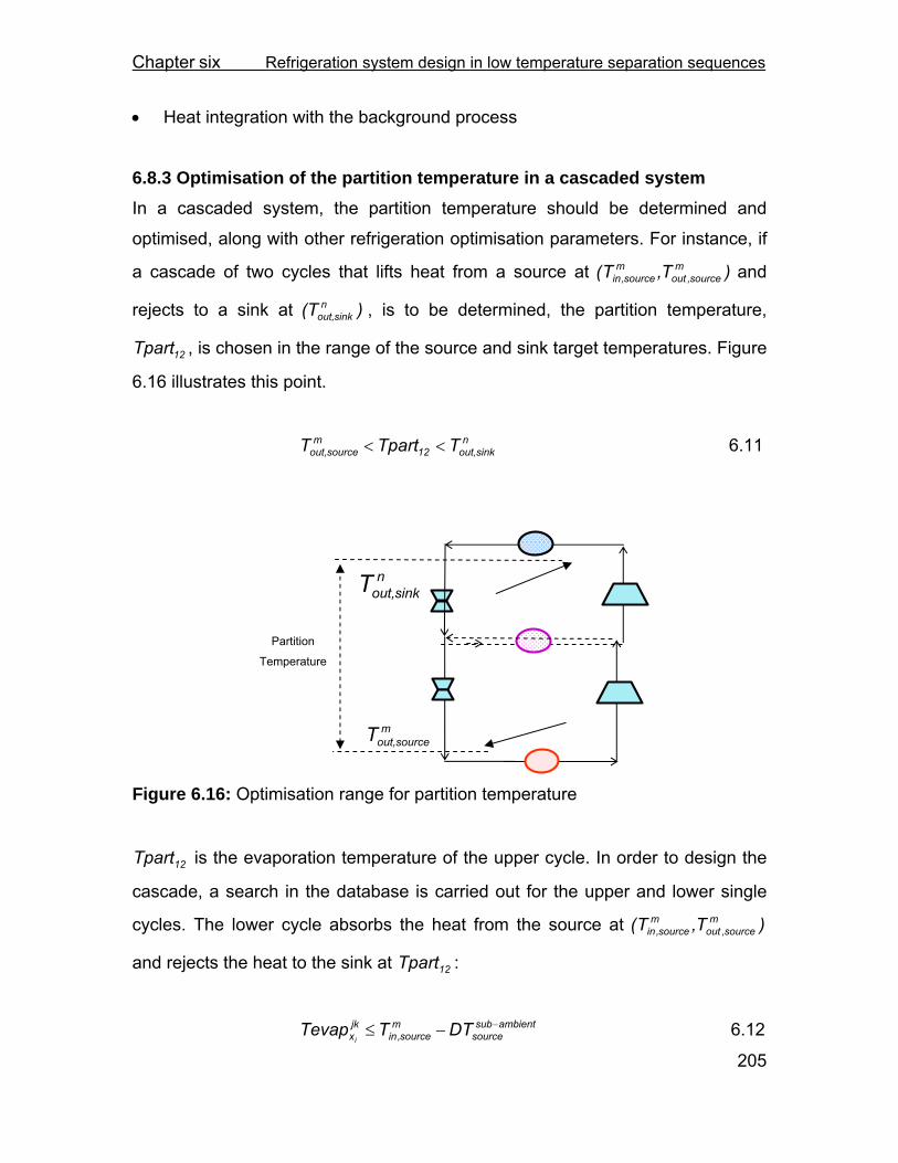
Chapter six Refrigeration system design in low temperature separation sequences
205
• Heat integration with the background process
6.8.3 Optimisation of the partition temperature in a cascaded system In a cascaded system, the partition temperature should be determined and
optimised, along with other refrigeration optimisation parameters. For instance, if
a cascade of two cycles that lifts heat from a source at )T,T( msource,out
msource,in and
rejects to a sink at )(T nsinkout, , is to be determined, the partition temperature,
12Tpart , is chosen in the range of the source and sink target temperatures. Figure
6.16 illustrates this point.
n
sinkout,12m
sourceout, TTpartT << 6.11
Figure 6.16: Optimisation range for partition temperature
12Tpart is the evaporation temperature of the upper cycle. In order to design the
cascade, a search in the database is carried out for the upper and lower single
cycles. The lower cycle absorbs the heat from the source at )T,T( msource,out
msource,in
and rejects the heat to the sink at 12Tpart :
ambientsub
sourcem
source,injkx DTTTevap
i
−−≤ 6.12
Partition
Temperature
msourceout,T
nsinkout,T

Chapter six Refrigeration system design in low temperature separation sequences
206
ambientsubsource
msource,out
jkx DTTTexp
i
−−≤ 6.13
sink12jkx DTTpartTcnd
i+≥ 6.14
The upper cycle absorbs heat from a source at 12Tpart and rejects heat to the
sink at )(T nsinkout, :
ambientsub
source12jkx DTTpartTevap
i
−−≤ 6.15
ambientsubsource12
jkx DTTpartTexp
i
−−≤ 6.16
sinkn
sinkout,jkx DTTTcnd
i+≥ 6.17
If no single cycle was found in the database that operates in the operating
temperature range of the lower cycle, )Tpart,T( 12m
source,out , the boundary for the
partition temperature range is modified as follows:
12
old
12
newm
source,out TpartTpartT << 6.18
A new partition temperature is chosen randomly in this range and the search for
the lower cycle continues. Also, if no single cycle is found that operates in the
operating temperature range of the upper cycle, )T,Tpart( nsinkout,12 , the boundary
for the partition temperature is again modified as follows:
nsinkout,12
new
12
oldTTpartTpart << 6.19
In this case, the search for both lower and upper cycles is repeated with the new
partition temperature.
Chapter six Refrigeration system design in low temperature separation sequences
207
Cascades with a maximum of three cycles are allowed in the present
methodology and their design procedure is similar to that of cascades of two
cycles. The reason for not allowing more than three cascades is to control the
complexity of the design. This will be further discussed in Section 6.9.2.1.
While the cost matrix is developed, a number of single cycles that are candidate
elements for the refrigeration system will be selected. Then the loads on the
matches between the source and sinks are optimised (Chapter 3). After load
optimisation, only simple cycles that belong to the matches with non-zero duty,
will be part of the final refrigeration system. Later, simple cycles with the same
refrigerant composition can be merged to form the multistage cycles.
6.9 Remarks 6.9.1 Parallel optimisation of the refrigeration and separation systems As mentioned in Section 6.8.1, for each match between the sources and sinks in
a sequence, a number, n, of feasible cycles from the database is examined and
the cycle with the smallest power consumption is chosen. The number, n, can be
chosen by the user to control the amount of optimisation of the refrigeration
system for each sequence. Moreover, in order to search the database efficiently,
the database is explored starting from a different point each time a search is
conducted. This allows a more thorough refrigeration system search.
It is not intended to optimise the refrigeration system for each separation
sequence. On the other hand, the refrigeration system will be optimised in
parallel to the optimisation of the separation sequence throughout the
optimisation. This avoids wasting optimisation time for optimising the refrigeration
system for a possibly non-optimum separation sequence.
6.9.2 Controlling the complexity of the design In order to control the complexity of the design, the maximum number of
refrigerant fluids and the maximum number of refrigeration levels are fixed.

Chapter six Refrigeration system design in low temperature separation sequences
208
6.9.2.1 Maximum number of refrigerant fluids
For controlling the maximum number of refrigerant fluids, while allocating cycles
to match a source with a sink, a record of the employed refrigerant fluids is kept.
If the number of utilised refrigerant fluids in the system at each trial solution
exceeds the maximum allowed, no more new refrigerant fluids will be selected.
Therefore, the search for cycles, for matching the remaining sources and sinks,
will be limited to the cycles of the present refrigerant fluids that operate between
different pressures.
In order to ensure that the refrigerants are capable of servicing other source and
sink matches, the coldest process source stream is first matched against the
hottest sink stream. An example is discussed to further elaborate this point. It is
assumed the available refrigerants can be pure or mixtures of methane, ethylene
and propylene. If the search algorithm starts providing cooling for the streams in
temperature ranges above the ethylene normal boiling point (~-102°C), the set of
refrigerants is likely to be filled with the mixtures of ethylene and propylene
(excluding methane). This set of refrigerants will not be able to cool a process
source at temperatures lower than -102°C, as they cannot provide a refrigerant
stream as cold as required. Therefore, infeasible solutions may occur in the
optimisation search procedure. In order to avoid infeasible solutions as far as
possible, source streams in the cost matrix are sorted in ascending order, while
the sink streams will be ranked in descending order. The search starts from
matching the coldest process source stream with the hottest sink stream first.
6.9.2.2 Maximum number of refrigeration levels
To restrain the maximum number of compression stages in the compressors, the
number of refrigeration levels is controlled. To do so, an MILP problem should be
formulated.
Chapter six Refrigeration system design in low temperature separation sequences
209
While the cost matrix is being determined, the set of potential pressure levels in
the heat pump system is formed. Each new pressure level, lxi
P , is distinguished
by the composition of the cycle iX and a value of pressure.
All the potential pressure levels, lxi
P , will not necessarily be present after
optimising the loads on the matches and generating the final design. If the load
on a match between source m and sink n is non-zero, then the corresponding
pressure levels should be activated and added to the refrigeration system.
A binary variable, mnlY , is allocated to each pressure level:
1,0Y mnl = 6.20
If a match, mn , is active, the associated binary variables to the pressure levels, mn
lY , involved in the heat pump system of the match will be one.
If 0Qmn > ⇒ 1Y mnl =
And, 6.21
If 0Qmn ≤ ⇒ 0Y mnl = , 1
The big-M method is used for mathematically representing these conditions.
0YMQ mnl
mn ≤×− 6.22
It should be mentioned that for each match at least two pressure levels and a
maximum of 6 pressure levels (for cascades of three cycles) may be involved.
The Constraint 6.23 is added to the heat exchanger network design problem to
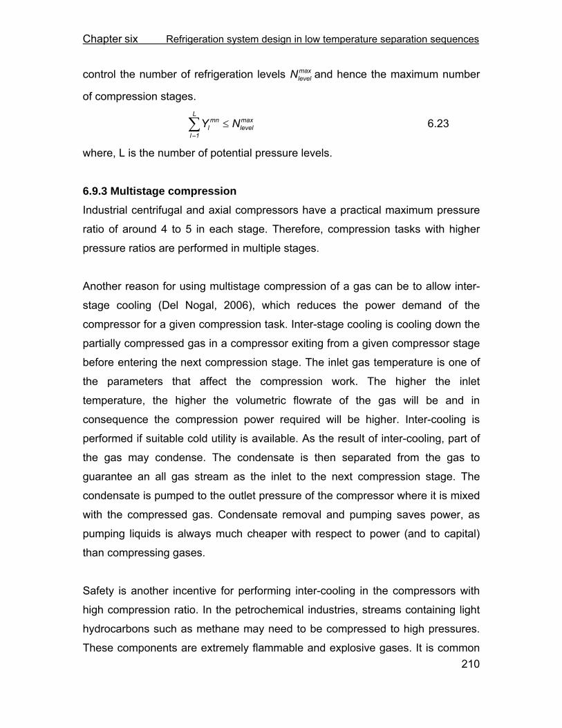
Chapter six Refrigeration system design in low temperature separation sequences
210
control the number of refrigeration levels maxlevelN and hence the maximum number
of compression stages.
maxlevel
L
1l
mnl NY ≤∑
=
6.23
where, L is the number of potential pressure levels.
6.9.3 Multistage compression Industrial centrifugal and axial compressors have a practical maximum pressure
ratio of around 4 to 5 in each stage. Therefore, compression tasks with higher
pressure ratios are performed in multiple stages.
Another reason for using multistage compression of a gas can be to allow inter-
stage cooling (Del Nogal, 2006), which reduces the power demand of the
compressor for a given compression task. Inter-stage cooling is cooling down the
partially compressed gas in a compressor exiting from a given compressor stage
before entering the next compression stage. The inlet gas temperature is one of
the parameters that affect the compression work. The higher the inlet
temperature, the higher the volumetric flowrate of the gas will be and in
consequence the compression power required will be higher. Inter-cooling is
performed if suitable cold utility is available. As the result of inter-cooling, part of
the gas may condense. The condensate is then separated from the gas to
guarantee an all gas stream as the inlet to the next compression stage. The
condensate is pumped to the outlet pressure of the compressor where it is mixed
with the compressed gas. Condensate removal and pumping saves power, as
pumping liquids is always much cheaper with respect to power (and to capital)
than compressing gases.
Safety is another incentive for performing inter-cooling in the compressors with
high compression ratio. In the petrochemical industries, streams containing light
hydrocarbons such as methane may need to be compressed to high pressures.
These components are extremely flammable and explosive gases. It is common

Chapter six Refrigeration system design in low temperature separation sequences
211
sense that having the gas with a high temperature at high pressure raises the
safety risks.
Figure 6.17 illustrates the impact of multistage compression with intercooling. A
mixture of hydrocarbons C1 to C4 is to be compressed from 1.01 bar and 30 °C
to 30 bar and 30 °C. The total compression ratio is 29.7 (01.1
30 ). In Figure 6.17-
(a), this task is carried out in a single compression stage. In Figure 6.17-(b) three
stages with inter-cooling are used for the same process. Three stages is the
minimum number of stages required to avoid compression ratios greater than 5.
An identical pressure ratio of 3.1 is assumed in all the stages.
Figure 6.17: Single stage compression versus multistage compression
The total compression power is reduced by 18% in the multistage compression
flowsheet with respect to the single stage flowsheet. A significant reduction in the
total cooling duty (16%) is also observed. The reduction in cooling duty is the
result of reducing power requirement. The inlet and outlet streams to both
flowsheets have identical conditions and therefore, the enthalpy change of the
inlet and outlet streams are the same in both cases. Hence, according to the
enthalpy balance (Qtot = Wtot – Hout + Hin), the extra energy in the form of
power input in the flowsheet of Figure 6.19 should be extracted in the after-cooler
to achieve the same enthalpy change.
1 bar 30 ˚C
1.6 kmol/s 30 ˚C 9.7 bar
108 ˚C 3.1 bar
Pr =29.7
30 ˚C 30 bar 274 ˚C
1 bar 30 ˚C
1.6 kmol/s
Pr = 3.1
30 ˚C 3.1 bar
109 ˚C 9.7 bar
111 ˚C 30 bar
30 ˚C 30 bar
Pr = 3.1 Pr = 3.1
Wtot = 18 MW Qtot = 20.4 MW Wtot = 22.1 MW Qtot = 24.4 MW
a) b)

Chapter six Refrigeration system design in low temperature separation sequences
212
6.10 Summary In this chapter a novel design approach for simultaneous synthesis and
optimisation of the design variables in heat integrated separation and
refrigeration systems is proposed. This robust methodology helps overcome the
complexities of heat integrated low temperature process design by using a
refrigeration system database and decomposition approach. The approach
overcomes challenges such as infeasible refrigeration system design and large
number of degrees of freedom in such processes.
Moreover, the approach is able to compare the performance of various
refrigeration provision strategies in different types of problems. Cascades of
multistage refrigeration cycles with both pure and mixed refrigerants can be
synthesised and optimised. In addition, the interactions between the separation
and refrigeration processes are considered and integration opportunities are
exploited.
Finally the refrigeration system design approach is capable of controlling the
complexity of the design by imposing constraints on the number of refrigerants
and refrigeration and rejection levels.
6.11 Nomenclature
powermnC
Cost of power demand of the heat pump system operating between
source stream m and sink stream n per unit heat load of source
stream m
hputilitymnC −
Cost of the ambient utility required for the heat pump system
operating between source stream m and ambient utility per unit heat
load of source stream m
totalmnC
Cost of utility for the match between source stream m and sink stream
n per unit heat load of source m
kj,
i
PXCyc
Simple refrigeration cycle with the refrigerant composition Xi and
lower and upper pressures equal to the pressures of element j,k of

Chapter six Refrigeration system design in low temperature separation sequences
213
the pressure set k,jP
DT Minimum approach temperature
ambientsubsourceDT −
Sub-ambient minimum approach temperature for process source
streams
f Objective function for minimising the utility cost
H Enthalpy
idealjkixHcmp
Ideal isentropic enthalpy at the exit of the compressor in the
refrigeration cycle kj,
i
PXCyc
realjkixHcmp
Real enthalpy at the exit of the compressor in the refrigeration cycle kj,
i
PXCyc
jkxi
Hevap Enthalpy at the exit of the evaporator in the refrigeration cycle kj,
i
PXCyc
n Counter for process streams maxlevelN Maximum number of pressure levels in the refrigeration system
SegmentsnP Number of pressure intervals for each refrigerant
P Pressure l
xiP Pressure levels of the refrigeration cycle
k,jP Set of lower and upper pressures in simple refrigeration cycles for
different compositions
LBxi
P Lower bound for pressure in a simple refrigeration cycle with
composition Xi
UBxi
P Upper bound for pressure in a simple refrigeration cycle with
composition Xi LL
j,xiP Lower pressure level in the refrigeration cycles with composition Xi
ULk,xi
P Upper pressure level in the refrigeration cycles with composition Xi
Q Heat duty
mnQ Heat load on the match mn
RA Rejects to ambient
RC Rejects to another refrigeration cycle
RP Rejects to process

Chapter six Refrigeration system design in low temperature separation sequences
214
jkxi
Sevap Entropy at the exit of the evaporator in the refrigeration cycle kj,
i
PXCyc
T Temperature
Tpart Partition temperature in the cascaded cycles
jkxi
Tcnd Condenser outlet temperature in the refrigeration cycle kj,
i
PXCyc
jkxi
Tevap Condenser outlet temperature in the refrigeration cycle kj,
i
PXCyc
jkxi
expT Expander outlet temperature in the refrigeration cycle kj,
i
PXCyc
jkxi
wComp Compressor power demand in the refrigeration cycle kj,
i
PXCyc
Xi Refrigerant composition set
mnlY Binary variable which indicates whether a pressure level l
xiP is active
Functions
sPT Returns the entropy of a stream given its composition, pressure and
temperature
hPS Returns the enthalpy of a stream given its composition, pressure and
entropy
hPT Returns the enthalpy of a stream given its composition, pressure and
temperature
Sub- and super- scripts
cond Condenser
evap Evaporator
in Inlet
j Counter for the pressure levels of the lower level in a simple refrigeration
cycle
k Counter for the pressure levels of the upper level in a simple refrigeration
cycle

Chapter six Refrigeration system design in low temperature separation sequences
215
LB Lower bound
LL Lower level in a simple refrigeration cycle
LOW_CYC Lower cycle in a cascaded refrigeration system
m Counter for process source streams
MIN Minimum
n Counter for process sink streams
out Outlet
source Process source streams
sink Process sink streams
sub-
ambient
Sub-ambient conditions
tot total
UB Upper bound
UL Upper level in a simple refrigeration cycle
UP_CYC Upper cycle in a cascaded refrigeration system
Greek letters
Δ Incremental change in the parameter
cη Isentropic efficiency in a compressor
Chapter seven Case studies in low temperature separation systems
216
7 Case studies in low temperature separation systems
7.1 Introduction In this chapter, the methodology proposed in this work is applied to two industrial
low temperature problems: separation of light hydrocarbons in an ethylene plant
and a liquefied natural gas (LNG) plant. The separation of light hydrocarbons
often demands high pressures and low temperatures and involves trains of
compressors and refrigeration systems to produce sub-ambient conditions. There
are complex interactions between the separation system, the compression
process, the refrigeration system and the heat exchanger network.
The approach in this work screens among various separation sequences and
considers both simple and complex distillation devices. Moreover, the feed and
product cooling, heating, compression and expansion processes are simulated,
evaluated, and included in the cost of the process. All process source and sink
streams (including feed and product streams) can exchange heat in parallel or
series heat exchanger arrangements with one another or with the external utility
in the HEN. An LP optimiser determines the optimum heat recovery network with
minimum utility cost. The HEN model also allows the interactions between the
separation and the refrigeration systems to be taken into account. An example of
such interactions is the trade-off between the choice of distillation column
operating pressure and the required refrigerated utility temperature. Moreover,
the methodology developed exploits the heat integration opportunities between
the separation and the refrigeration systems by allowing the refrigeration system
to reject heat at different temperature levels. Another point of strength for the
present model is that it considers different strategies for providing the required
refrigerated utility for the process. For instance, the refrigeration demand of the
process can be provided by expansion of a process stream, pure and mixed
multistage refrigeration systems or cascades of multistage refrigeration cycles.
Employing the enhanced simulated annealing (as the optimisation framework)

Chapter seven Case studies in low temperature separation systems
217
enables the methodology to tackle large industrial problems. In addition, the
optimisation framework optimises different variables in the separation and the
refrigeration systems simultaneously in order to minimise the operating cost of
the process. The complexity of the design can be controlled, in order to capture
the trade-offs between the capital and operating cost of the process. For
instance, the designer can choose the number of compression stages or the
number of refrigerant fluid types in the refrigeration system or the minimum heat
load on the heat exchangers in the HEN.
The strategy developed in this work is applied to the low temperature separation
problems, to demonstrate its effectiveness as the interactions between the
separation system, refrigeration system, compression process and heat recovery
network are systematically exploited.
7.2 LNG separation train Let us consider the separation of a heavy feed of an LNG (Liquefied Natural Gas)
plant. Prior to the liquefaction of the light end (mainly methane and ethane), it is
desired to separate the valuable heavy components. A typical specification of the
feed stream and products is shown in Table 7.1. Wang and Smith (2005)
minimised the operating cost for this LNG separation system and the result is
selected as the base case for this study.
7.2.1 Base case Wang and Smith (2005) minimise the operating cost for the separation problem
in Table 7.1. Regarding the methodology of Wang and Smith (2005), the
operating cost of the separation sequence is optimised and the separation
sequence and the refrigeration system are heat integrated employing heuristic
rules presented earlier in Chapter 6. Moreover, Wang and Smith (2005)
considered heat exchangers in parallel and did not allow series heat exchangers.
Overall, neither the heat recovery network nor the refrigeration systems were
optimised systematically. Only cascaded pure refrigeration systems were

Chapter seven Case studies in low temperature separation systems
218
considered by Wang and Smith (2005). The process for feed conditioning was
not considered in this work.
Table 7.1: Problem data for LNG separation train
i Component Fraction Product Product specification
1 Methane 0.3019
2 Ethane 0.2587 A • 99% recovery of ethane
• Saturated vapour at column pressure
3 Propane 0.2648 B • 98% purity of propane
• Saturated liquid at column pressure
4 Butane 0.1198 C • 98% purity of butane
• Saturated liquid at column pressure
5 Pentane 0.0358 D • 97% purity of pentane
• Saturated liquid at column pressure
6 Hexane 0.0190 E • 99% recovery of hexane
• Saturated liquid at column pressure
Flowrate 4313 kmol/h, saturated liquid at 5 bar
The optimisation parameters and conditions of Wang and Smith (2005) can be
highlighted as follows:
• the type of separation sequence is optimised;
• both simple and complex columns are taken into account;
• the operating pressure of all the separation units are optimised between 5
bar and 30 bar;
• the feed condition to the equipment is not optimised and set to be the
outlet condition from the upstream equipment or external feed condition;
• Condensing duty for a separation unit required below -40 ˚C is supplied by
ethylene-propylene cascaded refrigeration. A propylene single
refrigeration cycle is applied to provide cooling required above -40 ˚C;
• the available external utilities assumed by Wang and Smith (2005) are
listed in Table 7.2.
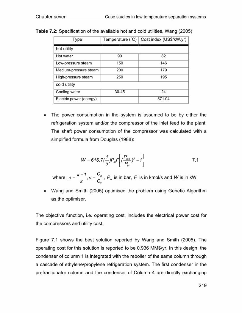
Chapter seven Case studies in low temperature separation systems
219
Table 7.2: Specification of the available hot and cold utilities, Wang (2005)
Type Temperature (˚C) Cost index (US$/kW.yr)
hot utility
Hot water 90 82
Low-pressure steam 150 146
Medium-pressure steam 200 179
High-pressure steam 250 195
cold utility
Cooling water 30-45 24
Electric power (energy) 571.04
• The power consumption in the system is assumed to be by either the
refrigeration system and/or the compressor of the inlet feed to the plant.
The shaft power consumption of the compressor was calculated with a
simplified formula from Douglas (1988):
⎥⎦
⎤⎢⎣
⎡−= 1)
PP(FP)1(7.616W
in
outin
δ
δ 7.1
where, v
p
CC
,1=
−= κ
κκδ , inP is in bar, F is in kmol/s and W is in kW.
• Wang and Smith (2005) optimised the problem using Genetic Algorithm
as the optimiser.
The objective function, i.e. operating cost, includes the electrical power cost for
the compressors and utility cost.
Figure 7.1 shows the best solution reported by Wang and Smith (2005). The
operating cost for this solution is reported to be 0.936 MM$/yr. In this design, the
condenser of column 1 is integrated with the reboiler of the same column through
a cascade of ethylene/propylene refrigeration system. The first condenser in the
prefractionator column and the condenser of Column 4 are directly exchanging

Chapter seven Case studies in low temperature separation systems
220
heat with the reboiler of Column 1 and the first reboiler of the prefractionator
column. It is reported that the rest of reboiler and condensers are serviced by
external utility.
Figure 7.1: The best solution reported by Wang and Smith (2005), for the problem in Table 7.1 In the next section, the LNG problem of Table 7.1 is optimised using the
methodology developed in this work. However, in order to have a meaningful
comparison, assumptions made in the base case and the case using the new
developed methodology should be unified as follows.
• Table 7.3 summarises the temperatures of the reboilers and the
condensers in Figure 7.1. The second condenser of the prefractionator
column is at 21.4 ˚C. In the design presented in Figure 7.1, this
condenser is serviced by external utility. However, the temperature of the
available ambient utility (cooling water) in Table 7.2 is higher than the
temperature of this condenser and hence cannot service it. If the
temperature of the cooling water is assumed to be lower than 21.4 ˚C by
at least one minimum approach temperature (to be able to accept heat
from the condenser of the prefractionator column), then cooling water
temperature will be lower than the temperature of the reboiler of Column
1. Hence, according to the Wang and Smith (2005) heuristics, the
refrigeration system should reject heat to cooling water instead of the
1
4
R1
Heat pumped from condenser to reboiler by
refrigeration cycles
Direct heat exchange between condenser and reboiler
Direct heat exchange between process stream and external utility
P1: 5.7 bar P2: 8.9 bar P3: 9.5 bar
2 3
A
B
C D
E

Chapter seven Case studies in low temperature separation systems
221
reboiler of Column 1, which is not the case as presented by Wang and
Smith (2005), Figure 7.1. Therefore, the temperature of the available
ambient utility should be determined. From now on, the ambient utility (i.e.
cooling water) is assumed to be heated from 20 ˚C to 30 ˚C. Table 7.4
shows the modified utility specifications.
Table 7.3: The temperatures of the condensers and reboilers of the sequence in Figure 7.1
Column Condenser temperature (˚C) Reboiler temperature (˚C)
Simple column 1 -67.6 20.5
Prefractionator column 2 31.4 89.0
Prefractionator column 3 21.4 128.7
Simple column 4 120.5 161.5
Table 7.4: Modified utility specifications of Wang and Smith (2005) Type Temperature (˚C) Cost Index (US$/kW.yr)
hot utility
Hot water 90 82
Low-pressure steam 150 146
Medium-pressure steam 200 179
High-pressure steam 250 195
cold utility
Cooling water 20-30 24
Electric power (energy) 571.04
• The simplified formula in Equation 7.1 for calculating the compressor
power does not have a consistent performance. In Table 7.5, the
compressor shaftwork calculated by Equation 7.1 is compared with the
shaftwork calculated using isentropic model in HYSYS for a number of
different inlet pressures and pressure ratios. Also, the size of the error is
shown in Table 7.5. This formula is clearly not reliable. Therefore, the
isentropic model (presented in Chapter 6) is employed for calculating the

Chapter seven Case studies in low temperature separation systems
222
compressor power demand in different parts of the process. An isentropic
efficiency of 0.87 is assumed for the compressor.
Table 7.5: Comparison between the values of compressor shaftwork calculated by Equation 7.1 and the isentropic model in HYSYS
Pin (bar) Pout/Pin WEquation 7.1 (kW) Wisentropic (kW) % (Wisentropic-WEquation 7.1)/ Wisentropic
2 2 906 1584 43
2 3 1487 2564 42
2 4 1924 3280 41
3 2 1359 1613 16
3 3 2231 2599 14
3 4 2885 3313 13
4 2 1813 1627 -11
4 3 2974 2612 -14
4 4 3847 3317 -16
• The operating pressure range of the problem is also modified from (5, 30)
bar to (5, 28) bar. The upper bound of 30 bar has been modified to be 28
to avoid operation at critical pressure of hexane, which is 30.32 bar.
Therefore, to have a fair comparison between the approach of Wang and Smith (2005) and the present approach, the best design of Wang and Smith (2005) is
re-simulated and re-evaluated, with the assumptions above. Figure 7.2 shows
the re-simulation of the design of Wang and Smith (2005) for the problem of
minimising the operating cost of the separation problem of Table 7.1. The
operating cost calculated for this sequence is 2.9 MM$/yr. In this design the
reboilers of Column 1 is employed as the heat sink for the refrigeration cycles
that service the condenser of Column 1 and the condenser of the main column in
the prefractionator Column 2. Also, the condenser of Column 4 and the
condenser of the prefractionator Column 3 are directly exchanging heat with the
reboilers in the separation sequence, as shown in Figure 7.2. The power demand
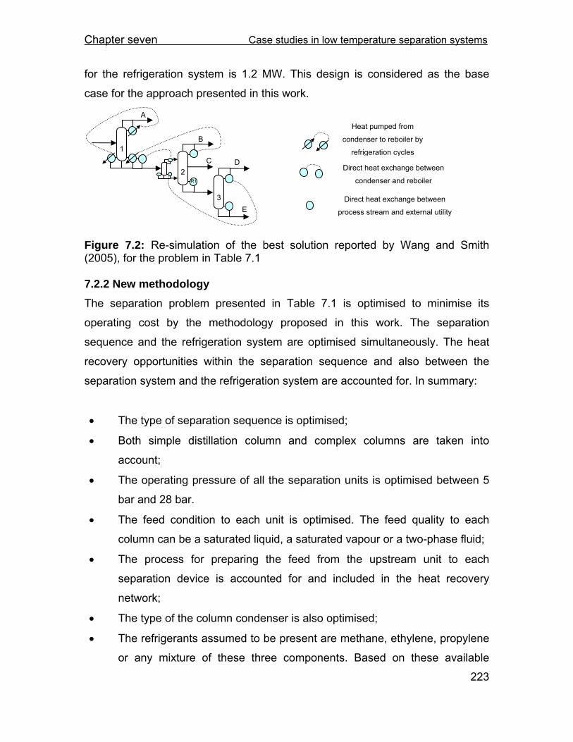
Chapter seven Case studies in low temperature separation systems
223
for the refrigeration system is 1.2 MW. This design is considered as the base
case for the approach presented in this work.
Figure 7.2: Re-simulation of the best solution reported by Wang and Smith (2005), for the problem in Table 7.1 7.2.2 New methodology The separation problem presented in Table 7.1 is optimised to minimise its
operating cost by the methodology proposed in this work. The separation
sequence and the refrigeration system are optimised simultaneously. The heat
recovery opportunities within the separation sequence and also between the
separation system and the refrigeration system are accounted for. In summary:
• The type of separation sequence is optimised;
• Both simple distillation column and complex columns are taken into
account;
• The operating pressure of all the separation units is optimised between 5
bar and 28 bar.
• The feed condition to each unit is optimised. The feed quality to each
column can be a saturated liquid, a saturated vapour or a two-phase fluid;
• The process for preparing the feed from the upstream unit to each
separation device is accounted for and included in the heat recovery
network;
• The type of the column condenser is also optimised;
• The refrigerants assumed to be present are methane, ethylene, propylene
or any mixture of these three components. Based on these available
2
1
3
R1
Heat pumped from
condenser to reboiler by
refrigeration cycles
Direct heat exchange between
condenser and reboiler
Direct heat exchange between
process stream and external utility
A
B
C D
E

Chapter seven Case studies in low temperature separation systems
224
refrigerants, a database is built with a composition interval size of 0.05,
pressure interval size of 1 bar for the pressures between 1 and 5 bar and
pressure interval size of 2 bar for cycle pressures above 5 bar. The
database includes 70449 simple cycles.
• In the refrigeration system the refrigerant composition, the pressure levels
and the partition temperature are optimised;
• Multistage compressors with inter-cooling are considered;
• The available external utilities assumed are listed in Table 7.4;
• The power consumption in the system is calculated using the isentropic
model with an efficiency of 0.87.
• The problem is optimised using the enhanced Simulated Annealing (SA)
presented in Chapter 5.
The objective function, i.e. the operating cost, includes the electrical power cost
for the compressors and the utility cost.
The best design for this optimisation is shown in Figure 7.3. The operating
conditions of the sequence are also presented in Figure 7.3. The sequence
presented does not require a refrigeration system and the sub-ambient cooling
duty is provided through heat integration with process sinks at below ambient
temperature. For instance, the saturated liquid feed to the plant is partly
vaporised to provide the sub-ambient cooling required in the condenser of the
columns and coolers in the system. This opportunity has been captured because
the optimisation framework considers the stream conditioning process and the
quality of the feed to the column is also optimised. Accounting for a two phase
feed to the column further optimises the temperature at which heating and
cooling is provided for the process. Moreover, the non-isothermal cooling,
heating and phase change of the streams are not neglected and this approach
has enabled the optimiser to capture further heat integration opportunities. For
instance, the feed to the plant is heated from -114 ˚C to 34 ˚C. If the stream
heating was considered isothermal, the temperature of the stream would have

Chapter seven Case studies in low temperature separation systems
225
been assumed to be 34 ˚C. Therefore, the optimiser could not heat integrate this
stream with the process sources at temperatures below 34 ˚C, while in practice
this stream can provide cooling at temperatures as low as -114 ˚C (plus the
minimum temperature approach). The operating cost of this system is 1.5
MM$/yr, which is significantly lower than the best design proposed by Wang and
Smith (2005).
Condenser Reboiler
Column Pressure
(bar)
Feed
quality T ( ˚C)Duty
MW T(˚C)
Duty
MW
Condenser
type
23 7.2 228 2.8 1
28
0.4
- - 143 2.4
Pc
2 5 0.5 -70 1.5 0.9 4.7 Pc
3 5 0.4 47 5.8 91 4.3 Tc
Objective value: 1.5 MM$/yr
Figure 7.3: Selected design for the problem in Table 7.1, using the developed methodology in the present work
1
2
3
1
2C1
R1
C2
R2 C3
R3
R12 3
A
BC
D
E
1
3
C1
R1
2
R12 R2
C2 C3
R3

Chapter seven Case studies in low temperature separation systems
226
In this separation problem, considering the feed conditioning process in the heat
recovery network allowed the system to capture the free refrigeration offered by
the feed to the plant. However, in practice the feed to the LNG separation train is
in vapour phase and prior to liquefying the light products in natural gas, it is
intended to separate the valuable heavy components. Therefore, in the next
section, the above problem is optimised assuming a saturated vapour feed to the
plant.
7.3 LNG separation train with vapour feed The feed and product conditions for the LNG separation problem are shown in
Table 7.6. The only difference with the separation problem presented in Section
7.2 is that the feed to the system is assumed to be saturated vapour. This
assumption is closer to the industrial practice. Table 7.4 shows the available
external utilities for this problem.
Table 7.6: Problem data for LNG separation train i Component Fraction Product Product specification
1 Methane 0.3019
2 Ethane 0.2587 A • 99% recovery of ethane
• Saturated vapour at column pressure
3 Propane 0.2648 B • 98% purity of propane
• Saturated liquid at column pressure
4 Butane 0.1198 C • 98% purity of butane
• Saturated liquid at column pressure
5 Pentane 0.0358 D • 97% purity of pentane
• Saturated liquid at column pressure
6 Hexane 0.0190 E • 99% recovery of hexane
• Saturated liquid at column pressure
Flowrate 4313 kmol/h, saturated vapour at 5 bar
The operating cost of the problem is minimised by two different methods. First,
the heuristic method of Wang and Smith (2005) is applied to generate the base
case. Secondly, the systematic approach developed in this work for simultaneous

Chapter seven Case studies in low temperature separation systems
227
design and optimisation of the refrigeration system and the separation sequence,
while considering the heat integration opportunities, is applied. The optimisation
framework in both cases is enhanced SA algorithm in Chapter 5. In both cases
the feed conditioning process is also accounted for.
7.3.1 Base case In summary,
• The type of separation sequence is optimised;
• Both simple and complex columns are taken into account;
• The operating pressure of all the separation units are optimised within the
range of 5-28 bar;
• The feed condition to the equipment is optimised to be either a saturated
liquid or a saturated vapour;
• Condensing duty for a separation unit required below -40 ˚C is supplied by
cascades of ethylene-propylene refrigeration cycles. A propylene single
refrigeration cycle is applied to provide cooling required above -40 ˚C.
• The power consumption in the system is calculated using energy balances
and equations of state, assuming an isentropic efficiency of 0.87.
The objective function, i.e. operating cost, includes the electrical power cost for
the compressors and utility cost.
Figure 7.4 shows the optimum sequence for this problem. Separation sequence
AB/CDE, A/B and C/D/E is selected. Overall, the sequence is operating at low
pressure, with a saturated vapour feed for Column 1 and Column 2 and saturated
liquid feed for Column 3. Wang and Smith (2005) do not allow for two-phase feed
to columns. For serving the condenser of Column 1 and Column 2, a refrigerated
utility is required. A simple propylene cycle and a cascade of ethylene-propylene
cycles are used to service these condensers. The cascaded cycles are
integrated with the reboiler of Column 2. This cascade takes advantage of the
process sink at below-ambient temperature and rejects part of the heat absorbed

Chapter seven Case studies in low temperature separation systems
228
from the condenser of Column 2 to the reboiler of Column 2. The rest of heat
loads on the refrigeration cycles are rejected to the cooling water. Also, the
remaining condenser and reboilers are served by the external utility. The
operating cost for this sequence is 7.6 MM$/yr and the total power demand for
the system is 9.7 MW.
Condenser Reboiler
Separation Pressure
(bar)
Feed
quality Temperature
˚C
Duty
(MW)
Temperature
˚C
Duty
(MW)
1 AB/CDE 6.3 0 -22.3 6.3 69.7 6.3
2 B/C 6.3 0 -65.4 6.5 8.5 2.1
3 C/D/E 5 1 49.7 3.2 130 7.6
Objective value: 7.6 MM$/yr
1
3
21
2C1
R1C3
R3
C2
R2
3
3: Dividing-wall column
A
B
C
D
E

Chapter seven Case studies in low temperature separation systems
229
Figure 7.4: Base case design for the problem in Table 7.6
The Wang and Smith (2005) methodology does not consider the non-isothermal
process streams. Therefore, all the refrigeration should be provided for the
condensers at the outlet temperature of the condenser, which is the coldest
temperature in condenser. Moreover, Wang and Smith (2005) do not optimise
any of the refrigeration optimisation variables. For instance, the partition
temperature in the cascaded cycles is fixed. Fixing the partition temperature,
when only few pure refrigerants are available and no constraints on the structure
of the refrigeration system are imposed, may be practical and not unreasonable.
However, when mixed refrigerants are considered and constraints on the number
of refrigeration levels are imposed, fixing the partition temperature is no longer
practical and accurate.
-68.4 ˚C
-47.8 ˚C
-43.8 ˚C
-25.3 ˚C
12.5 ˚C
40 ˚C

Chapter seven Case studies in low temperature separation systems
230
7.3.2 New methodology The optimisation specification for this problem is the same as the conditions
specified in Section 7.2.2. The optimum separation sequence is shown in Figure
7.5. The sequence A/BCDE, B/CDE, CD/E, and C/D of simple distillation
columns has been chosen. The operating cost of this sequence is 5.5 MM$/yr,
which shows a 29% saving compared to the base case. The total shaft power
demand for this system is 7.5 MW, 23 % lower than the base case.
In addition to systematically optimising the heat integration opportunities in the
overall process, there are a number of reasons why this work is capable of
improving the solutions. In the design of Figure 7.5, the quality of the feed to
Column 1 is optimised so that a two-phase stream is fed to this column. This has
reduced the load on the condenser of Column 1 compared to the condenser of
Column 2 in the base case, which carries out the similar separation task (A/B).
The cooling for the system in design of Figure 7.5 is required over a wider and
milder temperature range at feed stage. The model developed in this work is
capable of detecting this non-isothermal feed cooler stream and provides the
refrigeration required for this stream at multiple refrigeration temperature levels.
These strategies, together with exploiting the heat integration opportunities in the
separation sequence and between the separation and refrigeration systems,
have reduced the power demand of the process. For instance, the bottom
product of Column 1 is partially vaporised before being sent to the downstream
column to provide part of the cooling required for the inlet stream to the plant and
also accepting part of the heat rejected from the refrigeration system. The
reboiler of Column 1 is also heated up utilising the heat rejected from the
refrigeration system at sub-ambient temperature. The heat recovery network for
this design is shown in Figure 7.5. The chosen refrigeration system is a cascade
of an ethylene cycle against a multistage propylene cycle, as shown in Figure
7.5.
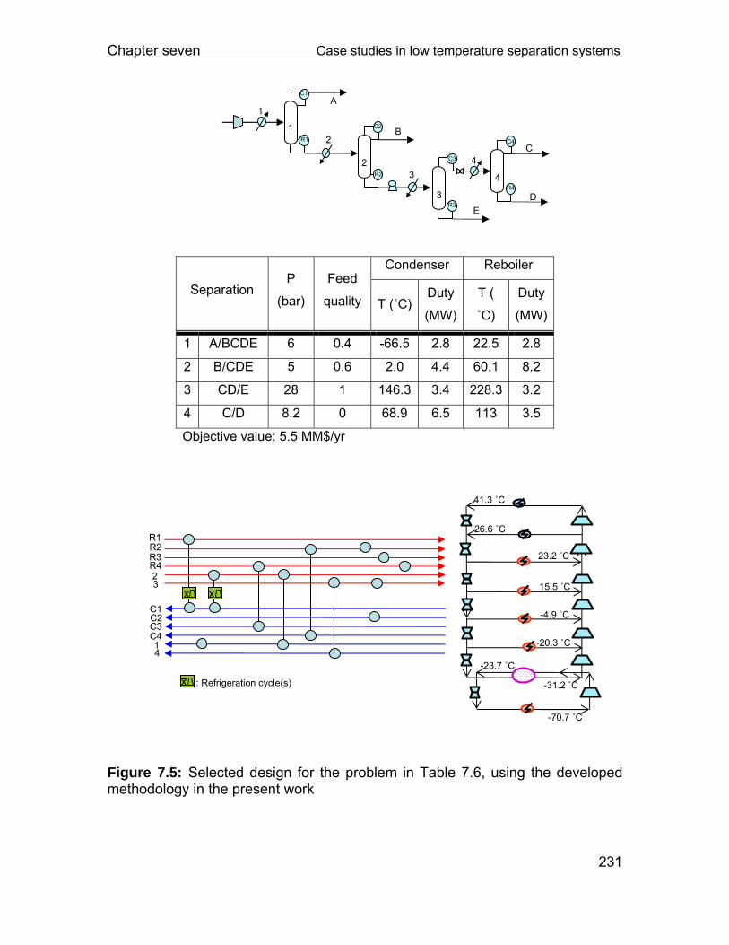
Chapter seven Case studies in low temperature separation systems
231
-70.7 ˚C
-31.2 ˚C
-23.7 ˚C
-4.9 ˚C
26.6 ˚C
41.3 ˚C
-20.3 ˚C
15.5 ˚C
23.2 ˚C
Condenser Reboiler
Separation P
(bar)
Feed
quality T (˚C)Duty
(MW)
T (
˚C)
Duty
(MW)
1 A/BCDE 6 0.4 -66.5 2.8 22.5 2.8
2 B/CDE 5 0.6 2.0 4.4 60.1 8.2
3 CD/E 28 1 146.3 3.4 228.3 3.2
4 C/D 8.2 0 68.9 6.5 113 3.5
Objective value: 5.5 MM$/yr
Figure 7.5: Selected design for the problem in Table 7.6, using the developed methodology in the present work
1
2
3
1
2
34
C1
R1
C2
R2
C3
R3
4
C4
R4
A
B
C
D
C4
4
C3
2
1
C1
R1 R2 R3
C2
R4
3
: Refrigeration cycle(s)
E

Chapter seven Case studies in low temperature separation systems
232
This study is carried out with an SA epoch length of 20, initial cooling parameter
of 0.05 and the minimum number of iterations of 4500. The computational time is
270 minutes on a Pentium® D processor (3.0 GHz) with 1 GB of RAM.
The effect of the size of the refrigeration system database on the problem
optimisation time is negligible. This is because very simple mathematical
calculations (e.g. addition and subtraction) are performed using the database.
However, the larger the size of the database is, the longer the required time for
building the database will be. Building a database of only pure components will
take few minutes, while building a database, which includes mixed refrigerants,
can take few hours, depending on how many temperature levels are considered.
The reported optimisation time in this thesis does not include the time required
for building the employed database. Once a database is built, it can be stored as
a data file and used in other problem optimisation tests. It should be noted that
the size of the database affects the quality of the solutions. This is apparent as
more refrigerant compositions and refrigeration temperature levels are explored
in larger refrigeration system database.
7.4 Ethylene cold-end separation In this section, the methodology developed will be applied to a more challenging
low-temperature separation problem. Thermal and steam cracking of mixtures of
ethane, propane and naphtha produces most of the global ethylene demand. The
product of the cracking furnaces is a gas mixture of mainly light hydrocarbons
and hydrogen. Separation of these light components requires a complex sub-
ambient utility system even at high pressure. The complexity and energy intensity
of this separation problem makes it an appropriate candidate for illustrating the
potential and effectiveness of the approach presented in this work. The study
employs the robust model of the present work to optimise the energy demand of
the separation train, while simultaneously accounting for the complex interactions
between the separation, refrigeration and the compression systems.

Chapter seven Case studies in low temperature separation systems
233
In the previous case studies in Section 7.2 and 7.3, no tight constraint was
imposed on the number of compression stages in the refrigeration system. There
are trade-offs between the complexity (together with the capital cost) of the
design and the operating cost of the process. These trade-offs can to some
extent be controlled by constraining the number of refrigeration pressure levels
and hence, the compression stages in the process; because compressor process
is responsible for a major part of the capital cost of the refrigeration system. In
this case study, a complex refrigeration system is required, as a large amount of
low-temperature cooling is expected to be demanded by the process. Therefore,
the number of refrigeration levels will be controlled in this case study.
The feed composition and the product recovery specifications are summarised in
Table 7.7. The composition of the gas mixture entering the separation train in an
ethylene plant strongly depends on the feedstock to the furnace. The feed
composition in Table 7.7 is based on a naphtha feed to the furnaces and is
obtained from Di Cintio et al. (1991).
Table 7.7: Problem data for ethylene cold-end separation
i Component Fraction Product Product specification
1 Hydrogen
2 Methane 0.35 A • 99% recovery of methane
• 10 bar, 30 ˚C
3 Ethylene 0.40 B • 99% purity ethylene
• 10 bar, Saturated liquid
4 Ethane 0.07 C • 99% recovery of ethane
• 10 bar, Saturated liquid
5 Propylene 0.11
6 Propane 0.01 D
• 98% recovery of propylene
• 10 bar, Saturated liquid
7 i-Butadiene 0.03
8 n-Butane 0.03 E
• 98% recovery of i-Butadiene
• 10 bar, 30 ˚C
Feed flowrate 5700 kmol/h, Vapour at 1.5 bar and 40 ˚C

Chapter seven Case studies in low temperature separation systems
234
Table 7.8: Available utility specifications
Type Temperature (˚C) Cost index (£/kW.yr)
hot utility
Hot water 90 25
Low-pressure steam 150 27.8
Medium-pressure steam 200 55.6
High-pressure steam 250 83.3
cold utility
Cooling water 20-30 33
Electric power (energy) 330
Due to its errant physical properties, hydrogen is treated as a non–condensable
component and it is assumed to be separated with methane in the light-end. The
optimisation specifications for this problem can be summarised as follows:
• The type of separation sequence is optimised;
• Both simple distillation column and complex columns are taken into
account;
• The operating pressure of all the separation units is optimised between 1
bar and 40 bar;
• The feed condition to each unit is optimised. The feed quality to each
column can be a saturated liquid, a saturated vapour or a two-phase fluid;
• The process for preparing the feed from the upstream unit to each
separation device is accounted for and included in the heat recovery
network;
• The type of the column condenser is also optimised;
• The refrigerants assumed to be present are methane, ethylene, propylene
or mixtures of these three components. Based on these available
refrigerants, a database is built with a composition interval size of 0.05,
pressure interval size of 1 bar for the pressures between 1 and 5 bar and
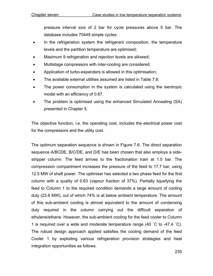
Chapter seven Case studies in low temperature separation systems
235
pressure interval size of 2 bar for cycle pressures above 5 bar. The
database includes 70449 simple cycles.
• In the refrigeration system the refrigerant composition, the temperature
levels and the partition temperature are optimised;
• Maximum 9 refrigeration and rejection levels are allowed;
• Multistage compressors with inter-cooling are considered;
• Application of turbo-expanders is allowed in this optimisation;
• The available external utilities assumed are listed in Table 7.8;
• The power consumption in the system is calculated using the isentropic
model with an efficiency of 0.87.
• The problem is optimised using the enhanced Simulated Annealing (SA)
presented in Chapter 5.
The objective function, i.e. the operating cost, includes the electrical power cost
for the compressors and the utility cost.
The optimum separation sequence is shown in Figure 7.6. The direct separation
sequence A/BCDE, B/C/DE, and D/E has been chosen that also employs a side-
stripper column. The feed arrives to the fractionation train at 1.5 bar. The
compression compartment increases the pressure of the feed to 17.7 bar, using
12.5 MW of shaft power. The optimiser has selected a two phase feed for the first
column with a quality of 0.63 (vapour fraction of 37%). Partially liquefying the
feed to Column 1 to the required condition demands a large amount of cooling
duty (23.6 MW), out of which 74% is at below ambient temperature. The amount
of this sub-ambient cooling is almost equivalent to the amount of condensing
duty required in the column carrying out the difficult separation of
ethylene/ethane. However, the sub-ambient cooling for the feed cooler to Column
1 is required over a wide and moderate temperature range (40 ˚C to -47.4 ˚C).
The robust design approach applied satisfies the cooling demand of the feed
Cooler 1 by exploiting various refrigeration provision strategies and heat
integration opportunities as follows.
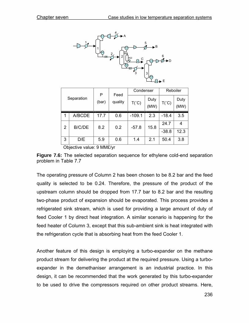
Chapter seven Case studies in low temperature separation systems
236
Condenser Reboiler
Separation P
(bar)
Feed
quality T(˚C) Duty
(MW)T(˚C)
Duty
(MW)
1 A/BCDE 17.7 0.6 -109.1 2.3 -18.4 3.5
24.7 4 2 B/C/DE 8.2 0.2 -57.8 15.8
-38.8 12.3
3 D/E 5.9 0.6 1.4 2.1 50.4 3.8
Objective value: 9 MM£/yr
Figure 7.6: The selected separation sequence for ethylene cold-end separation problem in Table 7.7
The operating pressure of Column 2 has been chosen to be 8.2 bar and the feed
quality is selected to be 0.24. Therefore, the pressure of the product of the
upstream column should be dropped from 17.7 bar to 8.2 bar and the resulting
two-phase product of expansion should be evaporated. This process provides a
refrigerated sink stream, which is used for providing a large amount of duty of
feed Cooler 1 by direct heat integration. A similar scenario is happening for the
feed heater of Column 3, except that this sub-ambient sink is heat integrated with
the refrigeration cycle that is absorbing heat from the feed Cooler 1.
Another feature of this design is employing a turbo-expander on the methane
product stream for delivering the product at the required pressure. Using a turbo-
expander in the demethaniser arrangement is an industrial practice. In this
design, it can be recommended that the work generated by this turbo-expander
to be used to drive the compressors required on other product streams. Here,
2
1
3
1 5C2
R2
C1
R1
C3
R3
R22
2
4
3
6
A
B
C D
E

Chapter seven Case studies in low temperature separation systems
237
product A is required at a lower pressure compared to the column operating
pressure. Reducing the pressure of the product from column operating pressure
to the required off-gas pressure decreases its temperature from -109 ˚C to -123
˚C and creates another sub-ambient heat sink for the process. The reboilers of
Columns 1, 2, and 3 are also providing part of the cooling required for the feed to
the plant both at sub- and above- ambient temperatures.
Moreover, in the design of Figure 7.6, the condenser of Column 3 is directly
exchanging heat with the reboiler of Column 1. The majority of the remainder of
the sub-ambient cooling required in the process is provided by the refrigeration
system.
The selected refrigeration system for this process is a cascade of pure and mixed
refrigeration cycles, as shown in Figure 7.7. A mixture of methane and ethylene
with the molar composition of methane 0.2 and ethylene 0.8 is used in the lower
cycle. This mixed refrigerant cycle absorbs heat from the condenser of Column 1
at -109 ˚C and rejects it to the first refrigeration level of the middle cycle in the
cascaded system, which is an ethylene cycle. Employing the mixed refrigeration
cycle has been chosen to reduce the number of refrigeration levels. The
condenser of Column 1 is operating out of the operating range of ethylene
refrigerant and hence, a methane cycle would be required if the mixed refrigerant
option was not available. The upper temperature bound for operation of a
methane cycle is almost -90 ˚C (to maintain an efficient latent heat and avoid
critical temperature at -83 ˚C), which is much colder than the temperature of the
first ethylene refrigeration level in design of Figure 7.7 (-61.9 ˚C). Hence, in case
where the refrigerant options were limited to pure components, another
refrigeration level and therefore, another compressor stage would be required in
the ethylene cycle. Employing mixed refrigerants has created opportunity to
reduce the complexity of the design (and hence the capital cost).
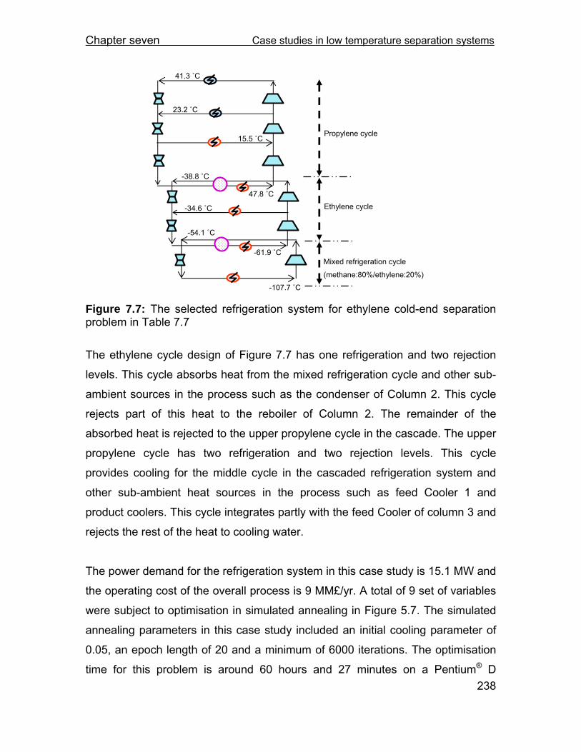
Chapter seven Case studies in low temperature separation systems
238
Figure 7.7: The selected refrigeration system for ethylene cold-end separation problem in Table 7.7
The ethylene cycle design of Figure 7.7 has one refrigeration and two rejection
levels. This cycle absorbs heat from the mixed refrigeration cycle and other sub-
ambient sources in the process such as the condenser of Column 2. This cycle
rejects part of this heat to the reboiler of Column 2. The remainder of the
absorbed heat is rejected to the upper propylene cycle in the cascade. The upper
propylene cycle has two refrigeration and two rejection levels. This cycle
provides cooling for the middle cycle in the cascaded refrigeration system and
other sub-ambient heat sources in the process such as feed Cooler 1 and
product coolers. This cycle integrates partly with the feed Cooler of column 3 and
rejects the rest of the heat to cooling water.
The power demand for the refrigeration system in this case study is 15.1 MW and
the operating cost of the overall process is 9 MM£/yr. A total of 9 set of variables
were subject to optimisation in simulated annealing in Figure 5.7. The simulated
annealing parameters in this case study included an initial cooling parameter of
0.05, an epoch length of 20 and a minimum of 6000 iterations. The optimisation
time for this problem is around 60 hours and 27 minutes on a Pentium® D
-107.7 ˚C
-61.9 ˚C
-54.1 ˚C
-38.8 ˚C
23.2 ˚C
41.3 ˚C
-34.6 ˚C
47.8 ˚C
15.5 ˚CPropylene cycle
Ethylene cycle
Mixed refrigeration cycle
(methane:80%/ethylene:20%)

Chapter seven Case studies in low temperature separation systems
239
processor (3.0 GHz) and 1 GB of RAM, with the majority of the optimisation time
spent on the design of the refrigeration system and heat recovery network.
7.5 Summary In this chapter, the developed methodology in this work for deign of heat
integrated low temperature distillation systems was applied to industrial case
studies with different complexity. The robustness of the approach was
demonstrated as it was capable of capturing the energy efficient design
opportunities specific to the conditions of each scenario. The key degrees of
freedom in the process screening stage in the separation system, such as
separation sequence and operating condition of separation devices (Wang,
2004), and the refrigeration system, such as refrigerant composition and the
refrigeration temperature levels (Del Nogal, 2006), are optimised simultaneously
using an enhanced simulated annealing algorithm. In addition, different
refrigeration provision strategies are available as design options in this
methodology. Moreover, heat integration opportunities within the separation
sequence and between the separation and refrigeration systems are considered.
The proposed designs in the case studies also reflect these features of the
developed model.

Chapter eight Conclusions and future work
240
8 Chapter 8 Conclusions and future work
8.1 Conclusions The present work has contributed to the design practice of low-temperature
separation processes by simultaneously optimising the key degrees of freedom
in the separation system and refrigeration systems. Moreover, the methodology
developed captures and exploits various complex interactions between the
separation and refrigeration systems.
Important design variables in the separation system, such as the separation
sequence, type and operating conditions of the separation units are optimised.
Both simple and complex distillation columns are taken into account. Moreover,
this work does not ignore the stream conditioning process. The feed and product
coolers, heaters, compressors and expanders are simulated; their costs are
evaluated, and included in the overall cost of the process. Dealing with the
stream conditioning processes provides a deeper insight into the design and
permits having greater confidence in the optimisation process. Chapter 2
discusses the above aspects of the present work.
Various refrigeration provision strategies are considered in the present work. For
instance, the refrigeration demand of the process can be provided by expansion
of a process stream, pure and mixed multistage refrigeration systems or
cascades of multistage refrigeration cycles. A novel approach based on
refrigeration system database is proposed, which overcomes the complexities
and challenges of synthesis and optimisation of refrigeration system (mainly due
to many infeasible designs) in the context of low-temperature separation process.
The methodology optimises the key design variables in the refrigeration system,
including the refrigerant composition, the number of compression stages, the
refrigeration and rejection temperature levels, cascading strategy and the

Chapter eight Conclusions and future work
241
partition temperature in multistage cascaded refrigeration systems. Chapter 6
expands on the refrigeration system synthesis model in this work.
Another major matter addressed in this work is the consideration of heat
integration opportunities within the separation sequence and between the
separation and refrigeration systems. It has been demonstrated that even though
low-temperature systems are highly energy intensive processes, there are
numerous opportunities for heat integrating the process and reduce the operating
cost of the system. Considering the heat integration opportunities in the synthesis
and optimisation of the refrigeration and separation systems increases the design
complexities of these already challenging design tasks significantly. The present
approach has selected a matrix based approach for assessing the heat
integration potentials of different separation and refrigeration systems in the
screening procedure. This approach captures the complicated interactions
between the separation and refrigeration systems through the heat exchanger
network robustly. Non-isothermal streams are not considered isothermal and
stream splitting and heat exchangers in series are taken into account. Chapter 3
describes the heat exchanger network design methodology.
Despite the fact that producing integrated separation and refrigeration systems is
attractive, in practice such task is challenging and requires a systematic
approach. This work combines a stochastic optimisation technique (enhanced
simulated annealing algorithm) and MILP optimisation method to develop a
framework for simultaneously optimising different degrees of freedom in the
process. Chapter 5 introduces this framework and extends the approach to the
design of heat integrated separation sequences in the above ambient
temperature process of benzene-toluene-xylene separation. The robustness of
the framework developed is further demonstrated in Chapter 7 where LNG
separation system and ethylene plant fractionation trains are studied. These case
studies demonstrated the strength of the methodology in considering the
effective refrigeration and integration strategies for servicing the large sub-

Chapter eight Conclusions and future work
242
ambient cooling demand of such processes. Finally, the studies establish that the
developed methodology allows the designer to analyse each specific separation
problem within its own context to develop understanding of the characteristics of
the problem in hand.
Chapter 4 of this thesis is dedicated to open loop heat pump assisted distillation
columns. Different scenarios with the potential of achieving higher energy
efficiency by using this technique are discussed. A shortcut model, consistent
with other process simulation approaches in this work, has been adopted for
simulation of heat pump assisted distillation columns. Case studies are
presented both at below and above ambient temperatures to demonstrate the
application of the developed model.
8.2 Future work This work optimises different degrees of freedom in the separation and
refrigeration processes simultaneously to minimise the operating cost of the
system. At present, the model is able to consider the capital cost of the system at
simulated annealing level. However, in order to claim simultaneity in the
optimisation of the design variables when studying the total cost of the system,
the capital cost of the heat exchanger network and refrigeration system
compressors should be considered at the MILP level, where the structure of the
heat recovery network is selected.
The present methodology considers heat exchangers in parallel and in series for
the process streams which allows fine optimisation of the heat recovery network.
Presently, the refrigeration system streams will exchange heat in parallel heat
exchangers. Considering heat exchangers in series for the refrigeration streams
can benefit the methodology by allowing it to exploit the sloped nature of mixed
refrigerant T-H curves even further. Moreover, although various refrigeration
provision strategies are considered in this work, incorporating closed loop
Chapter eight Conclusions and future work
243
expander cycles would allow all different refrigeration systems and major
technologies to be covered.
Another desirable extension area to the present work is considering more
separation options. For instance, sloppy split sequences can be added to the
present work. The sloppy split improves the separation efficiency by distributing
components between light and heavy key components. There are trade-offs
between the capital and operating costs when sloppy separation is applied,
which needs to be considered. Moreover, the present separation system design
methodology can include other equilibrium based separation methods, such as
absorption and extraction. In addition, the model can be taken one step further to
incorporate industrial designs specific to ethylene and LNG separation systems.
Examples of such state-of-art technologies include different demethaniser
flowsheets for enhancing ethylene recovery from the plant off-gas or
technologies for improving propane recovery in the de-ethaniser process. Also,
extending the present heat pump assisted distillation column to include columns
with partial condensers can be considered in the future.
Finally, applying stochastic optimisation tool creates higher chances of escaping
the local optima of the objective function. However, this is at the expense of long
computational time. As the complexity of the problem intensifies, the
computational time also increases significantly. The hybrid approach of using the
enhanced simulated annealing algorithm together with MILP approach improved
the optimisation procedure. However, it would be desired to further speed up this
process and investigate methods of achieving shorter computational time. For
instance, different algorithms of stochastic optimisation tools can be evaluated.
References
244
References
Aarts, E., H., L., and van Laarhoven, P., J., M., Statistical cooling: a general approach to combinatorial optimisation problems. Philips Journal of Research, vol. 40, iss. 4,193 -226, 1985. Agrawal, R., Woodward, D., W., and Yee, T., F., Argon production from air distillation: use of a heat pump in a ternary distillation with a sire rectifier. Gas Separation and Purification, 8(1), 37-43, 1994. Agrawal, R. and Yee, T., F., Heat pumps for thermally linked distillation columns: an exercise for argon production from air. Ind. Eng. Chem. Res., 33, 2717-2730., 1994 Aly, S., Heuristic approach for the synthesis of heat-integrated distillation sequences. International Journal of Energy Research, Vol. 21, 1297-1304, 1997. An., W., Yuan, X., Improved simulated annealing algorithm for synthesis of heat integrated distillation sequences, Huagong Xuebao/Journal of Chemical Industry and Engineering (China) 56 (3), 506-510, 2005. Annakou, O. and Mizsey, P., Rigorous investigation of heat pump assisted distillation. Heat Recovery Systems & CHP, 15(3), 241-247, 1995. Arau´joa, A., B., Britob, R., P., Vasconcelos, L., S., Exergetic analysis of distillation processes – A case study. Energy, 32, 1185–1193, 2007. Ashlock, D., Evolutionary Computation for Modeling and Optimization, Springer, 2006. Athier, G., Floquet, P., Pibouleau, L., and Domenech, S., Synthesis of heat-exchanger network by Simulated Annealing and NLP procedures. AIChE Journal, 43(11), 3007-3020, 1997. Balas, E., A note on duality in disjunctive programming. Journal of Optimisation Theory and Applications, 21 (4), 523-528, 1977. Biegler, L., T., and Grossmann, I. E., Retrospective on optimization. Comp. and Chem. Eng., 28, 1169–1192, 2004a. Biegler, L., T., and Grossmann, I. E., Part II. Future perspective on optimization. Comp. and Chem. Eng., 28, 1193–1218, 2004b. Bloch, H., and Soares, C., Turboexpanders and Process Applications. Gulf Professional Publishing, 2001. Blum, C. and Roli A., Metaheuristics in combinatorial optimization: Overview and conceptual comparison. ACM Computing Surveys, 35(3), 268–308, 2003.

References
245
Caballero, J., A., Grossmann, I., E., Aggregated models for integrated distillation systems. Ind. Eng. Chem. Res., Vol. 38, 2330-2344, 1999. Caballero, J., A., Grossmann, I., E., Structural considerations and modelling in the synthesis of heat integrated thermally coupled distillation sequences. Ind. Eng. Chem. Res., Vol. 45, 8454-8474, 2006. Carlberg, N., A. and Westerberg, A., W., Temperature heat diagrams for complex columns. 2: Underwood’s method for side strippers and enrichers. Ind. Eng. Chem. Res., 28, 1379-1386, 1989a. Carlberg, N., A. and Westerberg, A., W., Heat diagrams for complex columns. 3: Underwood’s method for the Petlyuk configurations. Ind. Eng. Chem. Res., 28, 1386-1397, 1989b. Carlsson, A., Franck, P. and Berntsson T., Design better heat exchanger network retrofits. Chemical Engineering Progress, 89(3), 87-96,1993. Cerda, J., Westerberg, A., W., Mason, D., and Linnhoff, B., Minimum utility usage in heat exchanger network synthesis - a transportation problem, Chem.Eng. Sci., 38(3), 373-387, 1983. Cerny, V., A thermodynamical approach to the travelling salesman problem: An efficient simulation algorithm. Journal of Optimisation Theory and Application, 45, 41–51, 1985. Ciric, A., and Floudas, C. A., A retrofit approach for heat exchanger networks. Comput. Chem. Eng., 13(6), 703-715,1989. Ciric, A., R., Floudas, C., A., Heat Exchanger Network Synthesis without Decomposition. Comps and Chem. Eng., 15(6), 385-396, 1991. Collura, M. A., and Luyben, W. L., Energy-saving distillation designs in ethanol production. Ind. Eng. Chem. Res., 27, 1686-1696, 1988. Colmenares, T., R., and Seider, W. D., Synthesis of cascade refrigeration systems integrated with chemical processes. Comp. Chem. Eng., Vol. 13(3), 247-258, 1989. Del Nogal, F., Optimal design and integration of refrigeration and power systems, PhD thesis, Department of Process Integration – University of Manchester Institute of Science and Technology (UMIST), UK, 2006. Demirhan, M., and O¨ zdamar, L., Experiments with new stochastic global optimisation search techniques. Computers and Operational Research, 27, 841–865, 2000. Di Cintio, R., Picciotti, M., Kaiser, V. and Pocini, C., A., Separation ethylene efficiently. Hydrocarbon processing, 70 (7), 83-90, 1991. Dolan, W., B., Cummings, P. T., LeVan, M., D., Process optimisation via simulated annealing: Application to network design, AIChE Journal, Vol. 35(5), 1989.

References
246
Douglas, J.M., 1988, Conceptual design of chemical processes, McGraw Hill Inc. Dr´eo, J., P´etrowski, A., Siarry, P., Taillard, E., Metaheuristics for hard optimization. Springer, 2006. Dueck, G. and Scheuer, T., Threshold accepting: a general purpose optimisation algorithm appearing superior to Simulated Annealing. Journal of Computational Physics, 90, 161-175, 1990. Elliot, J., R., and Lira, C., T., Introductory chemical engineering thermodynamics. Prentice Hall International Series in the Physical and Chemical Engineering Sciences, 1999. Energy technologies, Distillation heat pump configurations. http://tristate.apogee.net/et/eptsdco.asp. Energy Technology Support Unit (ETSU), Industrial refrigeration plant: energy efficient operation and maintenance. Energy Efficiency Office, Harwell, Oxon, 1992. Ferre, J.A., Castells, F., and Flores, J., Optimisation of a distillation column with a direct vapour recompression heat pump. Ind. Eng. Chem. Process Des. Dev., 24(1), 128-132, 1985. Flynn, T., Cryogenics Engineering. Second Edition ed., CRC Press, 2004. Floudas, C., A., Ciric, A., R., Strategies for Overcoming Uncertainties in Heat Exchanger Network Synthesis. Comps and Chem. Eng., 13(10), 1133-1152, 1989. Floquet, P., Pibouleau, L., and Domenech, S., Separation sequence synthesis: How to use simulated annealing procedure? Comps and Chem. Eng., Vol. 18, iss. 11-12, 1141-1148, 1994. Fonyo, Z., and Benko, N., Comparison of various heat pump assisted distillation configurations. Comp. Chem. Eng., 20(Suppl.) S85-S90, 1996. Fonyo, Z., and Benko, N., Enhancement of process integration by heat pumping, Trans IChemE, 76(A), 348-360, 1998. Fonyo, Z., and Miszey, P., Economic applications of heat pumps in integrated distillation systems. Heat Recording Systems & CHP, 14 (3), 249-263, 1994. Fraga, E., S., Zilinskas, A., Evaluation of hybrid optimisation methods for optimal design of heat integrated distillation sequences. Advances in Engineering Software, 34, 73-86, 2003. Furman, K., C., Sahinidis, N., V., A critical review and annotated bibliography for heat exchanger network synthesis in the 20th century. Ind. Eng. Chem. Res., Vol. 41, 2335-2370, 2002.
References
247
Gen, M., Cheng, R., Genetic Algorithms and Engineering Optimization, Wiley-IEEE, 2000. Glauber, R.J., Time-Dependent Statistics of the Ising Model. Journal of Mathematical Physics, 4(2), 294-207, 1963. Glinos, K. and Malone, M., F., Design of Side-stream Distillation Columns. Ind., Eng. Chem. Process Des. Dev., 24, 822-828, 1985. Goldberg, D., E., Genetic algorithms in search, optimisation, and machine learning, Addison-Wesley, Reading, Massachusetts, 1989. Grimes, L., E., Rychemer, M., D., and Westerberg, A., W., The synthesis and evolution of networks of heat exchange that feature the minimum number of units. Chem. Engng. Commun., Vol.14, iss. 3-6, 339-360, 1982. Grossmann, I. E., Caballero, J., A., Yeomans, H., Advances in mathematical programming for the synthesis of process systems, Latin American Applied Research, 30, 263-284, 2000. Gundersen, T., and Naess, L., The synthesis of cost optimal heat exchanger networks. Heat Recovery Systems & CHP, Vol 10 (4), 301-328, 1990. Hajek, B., Cooling schedule for optimal annealing. Mathematics of Operations Research, vol. 13, iss. 2, 311 -329, 1988. Hajek, B., and Sasaki, G., Simulated annealing - to cool or not. Systems and Control Letters, 12 (5), pp. 443-447, 1989. Haselden, G., G., Cryogenic fundamentals. Academic Press, London, New York, 12-15, 1971. Heckl, I., Friedler, F., and Fan, L., T., Integrated synthesis of optimal separation and heat exchanger networks involving separations based on various properties. Heat Transfer Engineering, Vol. 26, iss. 5, 25-41, 2005. Hedar, A., R., and Fukushima, M., Derivative-free filter simulated annealing method for constrained continuous global optimisation. Journal of Global Optimisation, 35, 521-549, 2006. Hendry, J., E., and Hughes, R., R., Generating separation process flowsheets. Chem.Eng. Prog., 68(6), 71-76, 1972. Henrich, F., Bouvy, C, Kausch, C., Lucas, K., PreuB, M., Rudolph, G., Roosen, P., Economic optimisation of non-sharp separation sequences by means of evolutionary algorithms. Comp. and Chem. Eng. Vol. 32, iss. 7, 1411-1432, 2008. Holiastos, K., Manousiouthakis, V., Minimum hot-cold and electric utility cost for a finite-capacity reservoir system. Comp. and Chem. Eng., 23, 1263–1276, 1999.

References
248
Holland, J., Adaptation in Natural and Artificial Systems, The University of Michigan Press, 1975. Jos, L. B., Polley, G., T., and Verheijen P. J. T., Structural targeting for heat integration retrofit. Applied Thermal Engineering, 18(5), 283-294,1998. Kerry, F., G., Industrial Gas Handbook: Gas Separation and Purification. CRC Press, 2007. King, C., J., Separation processes, 2nd ed., McGraw-Hill Inc., New York, 1980. Kirkpatrick, S., C., D., Gelatt and M., P., Vecchi, Optimisation by simulated annealing. Science, 220(4598), 671-680, 1983. Knuth, D. E., The art of computer programming. 2nd Edition, Addison-Wesley, London, 1981. Koehler, J.P., Aguirre, J.P. and Blass, E., Minimum reflux calculation for nonideal mixtures using the reversible distillation model. Chem. Eng. Sci., 46, 3007-3021, 1991. Koehler, J., P., Kuen, T. and Blass E., Minimum energy demand for distillation with distributed components and side-product withdrawals. Chem. Eng. Sci., 49, 3325-3330, 1994. Kovács, Z., Ercsey, Z., Friedler, F., and Fan, L., T., Separation-network synthesis: Global optimum through rigorous super-structure. Comp. and Chem. Eng., 24, 1881–1900, 2000. Leboreiro, J., Acevedo, J., Processes synthesis and design of distillation sequences using modular simulators: a genetic algorithm framework. Comp. & Chem. Eng., Vol. 28, 1223–1236, 2004. Lee, G., C., Optimal design and analysis of refrigeration systems for low temperature processes, PhD thesis, UMIST, UK, 2001. Lee, S., Grossmann, I., E., Global optimization of nonlinear generalized disjunctive programming with bilinear equality constraints: Applications to process networks. Comp. and Chem. Eng. 27 (11), 1557-1575, 2003. Lee, S., Grossmann, I., E., Generalized convex disjunctive programming: Nonlinear convex hull relaxation . Comp. and Chem. Eng. 26 (1), 83-100, 2003. Lewin, D., R, A generalized method for HEN synthesis using stochastic optimisation—II. The synthesis of cost-optimal networks. Comp. Chem. Eng., 22(10),1387–405, 1998. Linnhoff, B., Flower, J., R., synthesis of heat exchanger networks – 1. systematic generation of energy optimal networks. AIChE Journal, Vol. 24(4) 633-642, 1978. Linnhoff, B., Hindermarsh, E., The pinch design method for heat exchanger network. Chem. Eng. Sci., 38(5), 745-764, 1983.

References
249
Molokanov, Y., K., Korablina, T., P., Mazurina, N., I. and NiKiforov, G., A., An approximation method for calculating basic parameters of multicomponent fraction. Int. Chem. Eng., 12(2), 209-212, 1972. Markowski, M., Trafczynski, M., Urbaniec, K., Energy expenditure in the thermal separation of hydrocarbon mixtures using a sequence of heat-integrated distillation columns. Applied Thermal Engineering, 27, 1198–1204, 2007. Meszaros, I., Meili, A., 1-Butene separation processes with heat pump assisted distillation, Heat Recovery Systems & CHP, 14(3), 315-322, 1994. Mészáros, I., Fonyo, Z., Design strategy for heat pump assisted distillation systems, Heat Recovery Systems, 6(6) 469-476, 1986. Meili, A., and Stuecheli, A, Distillation columns with direct vapour recompression. Chemical Engineering, Feb, 1987. Mizsey, P., and Fonyo, Z., A predicted-based bounding strategy for synthesizing energy integrated total flowsheets. Comp. Chem. Eng., 14(11), 1303-1310, 1990. Metropolis, N., Rosenbluth, A., W., Rosenbluth, M., N., Teller, A., H., and Teller, E., Equation of state calculations by fast computing machines. Journal of Chemical Physics, 21(6), 1087-1091, 1953. Michalewicz, Z., Genetic Algorithms + Data Structures = Evolution Programs. Second ed., Berlin, Springer-Velag., 340, 1994. Mokhatab, S., and Economides, M., J., Process selection is critical to onshore LNG economics. World Oil, Feb, 2006. Mohan, S. and Vijayalakshmi, D., P., Estimation of Nash’s IUH parameters using stochastic search algorithms. Morari, M., and Faith, D., C., The synthesis of distillation trains with heat integration. AIChE Journal, 26, 916-928, 1980. Muhrer, C., A., Collura, M., A., and Luyben, W. L., Control of vapour recompression distillation columns. Ind. Eng. Chem. Res., 29, 59-71, 1990. Nishida, N., Stephanopoulos, G. and Westerberg, A., W., A review of process synthesis. AIChE. Journal 17, 321-351, 1981. Oliveira, S., B., M., Marques, M. P., and Parise, J. A. R., Modelling of an ethanol-water distillation column with vapour recompression. Int. J. Energy Res., 25, 845-858, 2001. Olujić, Ž., Sun, L., de Rijke, A. , and Jansens, P., J., Conceptual design of an internally heat integrated propylene-propane splitter. Energy, 31, 3083-3096, 2006.

References
250
Papalexandri, K., P., Pistikopoulos, E., Generalized modular representation framework for process synthesis. AIChE Journal, Vol. 42, No. 4, 1010-1032, 1996. Pedamallu, C., S., and Ozdamar, L., Investigating a hybrid simulated annealing and local search algorithm for constrained optimisation. European Journal of Operational Research, 185, 1230-1245, 2008. Pibouleau, L., Floquet, P. and Domenech, S., Fuzziness and branch and bound procedures: applications to separation sequencing. Fuzzy Sets and Systems, 109, 111-127, 2000. Papoulias, S.A., and Grossmann, I. E., A structural optimization approach in process synthesis-II. Heat recovery networks, Comp.. Chem. Eng., 7(6), 707-721, 1983. Raman, R., Grossmann, I., E., Relation between MILP modelling and logical inference for chemical process synthesis. Comp. and Chem. Eng., 15 (2), 73-84, 1991. Raman, R., Grossmann, I., E., Integration of logic and heuristic knowledge in MINLP optimization for process synthesis. Comp. and Chem. Eng., 16 (3), 155-171, 1992. Raman, R., Grossmann, I., E., Symbolic integration of logic in mixed-integer linear programming techniques for process synthesis. Comp. and Chem. Eng., 17 (9), 909-927, 1993. Raman, R., Grossmann, I., E., Modelling and computational techniques for logic based integer programming . Comp. and Chem. Eng., 18 (7), 563-578, 1994. Rastogi, V., Heat-integrated crude oil distillation system design. PhD Thesis, Department of Process Integration – University of Manchester Institute of Science and Technology (UMIST), 2006. Rathore, R., N., S., Wormer, K., A., V. and Powers, G., J., Synthesis strategies for multicomponent separation systems with energy integration. AIChE Journal, Vol. 20, No. 3, 491-502, 1974. Robbins, H. and Monro, S., A Stochastic Approximation Method, Annals of Mathematical Statistics, vol. 22, 400-407, 1951. Robinson, C., S. and Gilliland, E., R., Element of fractional distillation. 4th Ed, McGraw-Hill, New York, 1950. Samanta, A., Modelling and optimisation for synthesis of heat integrated distillation sequences in the context of the overall process, PhD thesis, Department of Process Integration – University of Manchester Institute of Science and Technology (UMIST), UK, 2001. Schwefel, H., Numerical optimization of computer models. New York: Wiley, 1991. Seader, J., D. and Henley, E., J., Separation process principles. John Wiley& Son Inc., New York, 1998.
References
251
Seader, J., D., and Westerberg, A. W., A combined heuristic and evolutionary strategy for synthesis of simple separation sequences. AIChE Journal, 23, 951, 1977. Shah, P., 1999, Conceptual programming: a new approach for the optimisation, analysis and novel development of simple and complex separation systems. PhD thesis, Department of Process Integration – University of Manchester Institute of Science and Technology (UMIST), UK, 1999. Shelton, M., R., Grossmann, I., E., A shortcut procedure for refrigeration systems. Comp. and Chem. Eng., 9 (6), 615-619, 1985. Shelton, M., R., Grossmann, I., E., Optimal synthesis of integrated refrigeration systems-I. Mixed-integer programming model. Comp. and Chem. Eng., 10 (5), 445-459, 1986a. Shelton, M., R., Grossmann, I., E., Optimal synthesis of integrated refrigeration systems-II. Implicit enumeration scheme. Comp. and Chem. Eng., 10 (5), 461-477, 1986b. Shokoya, C. G., Retrofit of heat exchanger networks for debottlenecking and energy savings. PhD Thesis, Department of Process Integration – University of Manchester Institute of Science and Technology (UMIST), 1992. Silangwa, M., Evaluation of various surface area efficiency criteria in heat exchanger network retrofits, MSc. Thesis, Department of Process Integration – University of Manchester Institute of Science and Technology (UMIST), UK,1986. Sloley, A. W., Distillation operations manual. The Distillation Group Inc, 2001. Smith, R., Chemical process design and integration, John Wiley & Sons, New York, 2005. Stupin, W., J., Lockhart, F., J., Thermally coupled distillation- A case history. Chem. Eng. Prog., Vol. 68, 71-72, 1972. Tedder, D.W. and Rudd, D.F., Parametric studies in industrial distillation, AIChE J., 24, 303-315, 1978. Tjoe, T. N., and B. Linnhoff, Using pinch technology for process retrofit. Chemical Engineering, April, (28), 47-60,1986. Triantafyllou, C., The design, optimization and integration of dividing wall columns. PhD thesis, UMIST, UK, 1991. Triantafyllou, C. and Smith, R., The design and optimisation of fully thermally coupled distillation columns. Trans. Inst. Chem. Eng., 70, 118-131, 1992. Turkay, M., Grossmann, I., E., Logic-based MINLP algorithms for the optimal synthesis of process networks. Comp. and Chem. Eng. 20 (8), 959-978, 1996.

References
252
Umeda, T., Niida, K. and Shiroko, K., A thermodynamic approach to heat integration in distillation systems. AIChE Journal, 25, 423-429, 1979. Vaidyaraman, S. and Maranas, C.D., Optimal synthesis of refrigeration cycles and selection of refrigerants, AIChE Journal 45 (5), 997-1017, 1999. Vaidyaraman, S. and Maranas, C.D., Synthesis of mixed refrigerant cascade cycles, Chemical Engineering Communications, Vol. 189, No. 8, 1057-1078, 2002. Varbanov, P. S., and Klemes, J., Rules for paths construction for HENs debottlenecking. Applied Thermal Engineering, 20, 1409-1420, 2000. Wallin, E. and Berntsson T., Integration of heat pumps in industrial processes. Heat recovery systems & CHP, Vol.14, iss. 3, 287-296, 1994. Wang, J., Synthesis and optimisation of low temperature gas separation processes. PhD Thesis, Department of Process Integration – University of Manchester Institute of Science and Technology (UMIST), 2004. Wang, J., Smith, R., Synthesis and optimization of low-temperature gas separation processes. Ind. Eng. Chem. Res., Vol. 44, iss. 8, 2856-2870, 2005. Wang, K., Qian, Y., Yuan, Y. and Yao, P., A systematic modelling framework of superstructure optimization in process synthesis. Comp. & Chem. Eng., Vol. 23, 125-136, 1998. Wang, X.,H., Li, Y., G., Hua, Y., D., Wang, Y., L., Synthesis of heat-integrated complex distillation systems via Genetic Programming. Comp. Chem. Eng., 32,1908–1917, 2008. Westerberg, A., W., The synthesis of distillation-based separation systems. Comp. Chem. Eng., 9, 421-429, 1985. Wu, G. D., Design and retrofit of Integrated refrigeration Systems. PhD Thesis, Department of Process Integration – University of Manchester Institute of Science and Technology (UMIST), 2000. Wu, G. D., Zhu, X. X., Design of Integrated refrigeration Systems. Ind. Eng. Chem. Res., 41, 553-571, 2002. Yee, T., F., and I., E. Grossmann, A screening and optimisation approach for the retrofit of heat-exchanger networks, Ind. Eng. Res., 30, 146-162,1991. Yeomans, H., Grossmann, I., E., A systematic modelling framework of superstructure optimization in process synthesis. Comp. & Chem. Eng., Vol. 23, iss. 6, 709-731, 1999a. Yeomans, H., Grossmann, I., E., Nonlinear disjunctive programming models for the synthesis of heat integrated distillation sequences. Comp. & Chem. Eng., Vol. 23, iss. 9, 1135-1151, 1999b.

References
253
Yeomans, H., Grossmann, I., E., Disjunctive programming models for the optimal design of distillation columns and separation sequences. Ind. Eng. Chem. Res., Vol. 39, iss. 6, 1637-1648, 2000a. Yeomans, H., Grossmann, I., E., Optimal design of complex distillation columns using rigorous tray-by-tray disjunctive programming models. Ind. Eng. Chem. Res., 39, iss. 11, 4326-4335, 2000b. Yuan, X., An, W., Synthesis of heat integrated complex distillation systems visa stochastic optimisation approaches. Chinese Journal of Chemical Engineering 10 (5), 495-507, 2002. Zhang, L., Linninger, A., A., Towards computer-aided separation synthesis. AIChE Journal, Vol. 52, No 4, 1392–1409, 2006. Zhu, X. X, Zanfir, M. and Klemes, J., Heat transfer enhancement for heat exchanger network retrofit. Heat Transfer Engineering, 21(2), 7-18, 2000.

Appendix A Stream conditioning process
254
A. Appendix A Various stream conditioning scenarios
In this section, the strategy of this work for simulating and evaluating the feed
conditioning process is explained. It is assumed that the products from each
column are at the saturated conditions at the column pressure. The feed to
each column can be a saturated liquid, saturated vapour or two-phase fluid.
Sub-cooled or superheated feed is not considered in order to control the
complexity of the problem. Moreover, introducing sub-cooled or superheated
vapour increases either reboiler or condenser load in the distillation column as
it participates in the distillation process after it reaches the saturation
conditions. Table A.1 summarises different possible scenarios.
Table A.1: Different scenarios for the stream conditioning process in a
separation sequence
Scenario Upstream Product Condition Downstream Feed Condition Pressure Change
1 Saturated Liquid Saturated Liquid P1 > P2
2 Saturated Liquid Saturated Liquid P1 < P2
3 Saturated Liquid Saturated Vapour P1 > P2
4 Saturated Liquid Saturated Vapour P1 < P2
5 Saturated Vapour Saturated Liquid P1 > P2
6 Saturated Vapour Saturated Liquid P1 < P2
7 Saturated Vapour Saturated Vapour P1 > P2
8 Saturated Vapour Saturated Vapour P1 < P2
9 Saturated Liquid Two-phase Fluid P1 > P2
10 Saturated Liquid Two-phase Fluid P1 < P2
11 Saturated Vapour Two-phase Fluid P1 > P2
12 Saturated Vapour Two-phase Fluid P1 < P2

Appendix A Stream conditioning process
255
A.1 Scenario 1: Saturated Liquid to Saturated Liquid, P1 > P2 Scenario 1 was discussed in Chapter 2. As it was concluded, sub-cooling the
saturated liquid feed at higher pressure and expanding the sub-cooled liquid
is the promising choice economically and is implemented in this work.
A.2 Scenario 2: Saturated Liquid to Saturated Liquid, P1 < P2 Scenario 2 is a straightforward operation. The input to the transition box in
Figure A.1 is a saturated liquid and the output, which is the feed to the
upstream, is a saturated liquid at a higher pressure.
Figure A.1: Scenario 2 of Table A.1
To deliver the feed to the downstream process, first its pressure is raised in a
pump and then it is heated to saturation condition. Pumping the liquid is a
cheap process. Any order of heating and pumping the liquid will result in
almost the same cost, and hence, the order is unimportant.
A.3 Scenario 3: Saturated Liquid to Saturated Vapour, P1 > P2 In Scenario 3, a saturated liquid stream is transformed to a saturated vapour
stream at a lower pressure (the dashed arrow ac in Figure A.2). Two paths
are possible for this change:
1. expansion of the saturated liquid to the desired pressure and heating
the resulted two-phase mixture to generate saturated vapour, path abc
in Figure A.2;
or,
2. evaporation of the saturated liquid and expanding the vapour to the
desired pressure, either through a turbo expander or a throttle valve,
path ab’c in Figure A.2.
Transition
Box
Sat. Liq. at P1 Sat. Liq. at P2 P1<P2

Appendix A Stream conditioning process
256
Figure A.2: Temperature-enthalpy curve for Scenario 3
The net energy required for this change (from saturated liquid to the saturated
vapour feed at a lower pressure) would be the same, regardless of the chosen
path. The difference between the two paths is in the quality of the required
energy. In an above ambient process, path 1 may become a more promising
option, as the isenthalpic expansion of the saturated liquid produces some
vapour. Also, the temperature of the fluid drops as the result of expansion.
Therefore, having to heat and vaporise a colder fluid, a less expensive hot
utility will be required. In the second option, the vaporisation is required at a
higher temperature. Even though the latent heat of vaporisation is lesss at
higher pressures, high quality utility is more expensive. However, if the
process operation conditions justify employing a turbo expander, then the
economic benefit of generating work in the turbo expander may push towards
applying the second option. Installing a turbo expander may be an attractive
option when the expander generates a considerable amount of work, which
can be used in the plant.
In a below ambient process, both paths may be promising options, depending
on the process and the pressure drop. If the first path is chosen, the pressure
drop in the throttle valve will generate a colder cold stream (i.e. a stream that
needs to be heated up with a sub-ambient temperature). The refrigeration,
T Lines of constant
pressure
a
b c
H
P1
P2
b’

Appendix A Stream conditioning process
257
provided by this cold stream, can be heat integrated with other streams in the
process and can introduce savings to the system by reducing the load of the
refrigeration system.
On the other hand, the second path can install a turbo expander in the
process. There are two benefits in applying a turbo expander. First, work can
be generated by expanding the vapour from the higher pressure to the lower
one. Secondly, a turbo expander operates isentropically. Therefore, it can
reduce the temperature of the fluid considerably and hence, a better
refrigerant (i.e. a colder refrigerant) will be produced. Again, whether the
application of a turbo expander (i.e. its capital cost) is justified or not, depends
on the process operating conditions and demands.
In this work, the first option is implemented for transforming a saturated liquid
stream to a saturated vapour stream at a lower pressure. Two reasons
support this decision:
1. Option 1 can perform well both below and above ambient temperature.
2. The second option requires not only the turbo expander but also
demands more heat exchanger area, which results in a higher capital
cost.
A.4 Scenario 4: Saturated Liquid to Saturated Vapour, P1 < P2 In Scenario 4, two paths are possible. In path 1, the liquid is evaporated
through a heater and the saturated vapour is compressed in a compressor
and then de-superheated. This is the abcd path shown on the Figure A.3. This
will not be the most efficient path, because:
1. the latent heat of vaporisation of the fluid at the lower pressure is
higher than the latent heat of vaporisation of the fluid at the higher
pressure.
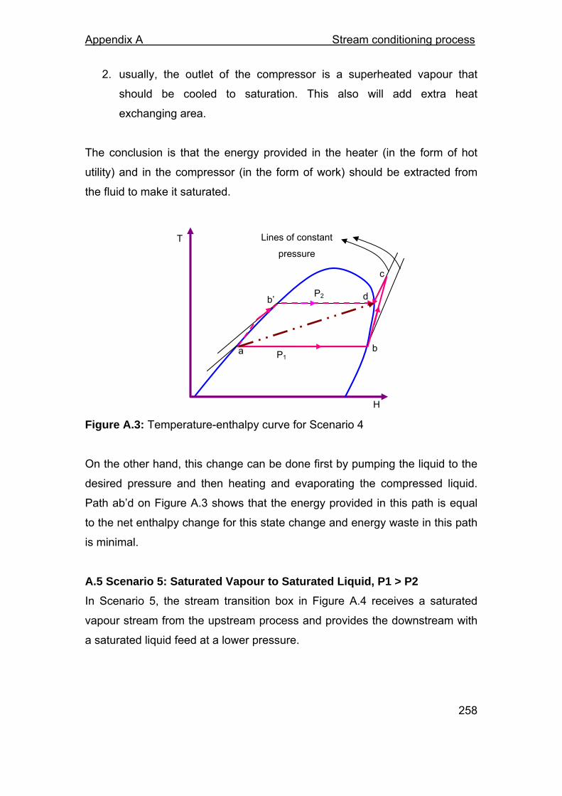
Appendix A Stream conditioning process
258
2. usually, the outlet of the compressor is a superheated vapour that
should be cooled to saturation. This also will add extra heat
exchanging area.
The conclusion is that the energy provided in the heater (in the form of hot
utility) and in the compressor (in the form of work) should be extracted from
the fluid to make it saturated.
Figure A.3: Temperature-enthalpy curve for Scenario 4
On the other hand, this change can be done first by pumping the liquid to the
desired pressure and then heating and evaporating the compressed liquid.
Path ab’d on Figure A.3 shows that the energy provided in this path is equal
to the net enthalpy change for this state change and energy waste in this path
is minimal.
A.5 Scenario 5: Saturated Vapour to Saturated Liquid, P1 > P2 In Scenario 5, the stream transition box in Figure A.4 receives a saturated
vapour stream from the upstream process and provides the downstream with
a saturated liquid feed at a lower pressure.
a b
c
T
H
P1
P2 b’ d
Lines of constant
pressure
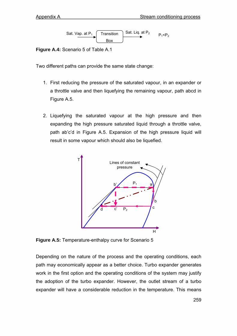
Appendix A Stream conditioning process
259
Figure A.4: Scenario 5 of Table A.1
Two different paths can provide the same state change:
1. First reducing the pressure of the saturated vapour, in an expander or
a throttle valve and then liquefying the remaining vapour, path abcd in
Figure A.5.
2. Liquefying the saturated vapour at the high pressure and then
expanding the high pressure saturated liquid through a throttle valve,
path ab’c’d in Figure A.5. Expansion of the high pressure liquid will
result in some vapour which should also be liquefied.
Figure A.5: Temperature-enthalpy curve for Scenario 5
Depending on the nature of the process and the operating conditions, each
path may economically appear as a better choice. Turbo expander generates
work in the first option and the operating conditions of the system may justify
the adoption of the turbo expander. However, the outlet stream of a turbo
expander will have a considerable reduction in the temperature. This means
Transition
Box
Sat. Vap. at P1 Sat. Liq. at P2 P1<P2
a
b c
T
H
P1
P2
Lines of constant pressure
b’
c’ d
Appendix A Stream conditioning process
260
the liquefaction of the resulting two-phase fluid should be carried out at a
lower temperature. In a below ambient process, a more expensive
refrigeration temperature will be required for this purpose. In the second
option, the majority of the duty is rejected at a higher temperature for
liquefying the vapour, potentially resulting in a cheaper process, as cheaper
utility will be needed. In an above ambient process, also, rejection of the heat
at a higher temperature may be more attractive, since there will be
opportunities for heat integration.
Overall, unless the production of work by the turbo expander is of interest to
the system, and the trade-offs between the operating and capital cost can be
justified, the second path seems more economically attractive.
In this work, if the user chooses to allow turbo expander in the process, then
the first option is selected. Otherwise, first the vapour is cooled at the high
pressure and temperature and then its pressure is dropped in a throttle valve.
A.6 Scenario 6: Saturated Vapour to Saturated Liquid, P1 < P2 In performing Scenario 6, changing a saturated vapour to a saturated liquid at
a higher pressure, the options are:
1. first, compress the saturated vapour in a compressor to the desired
pressure; and then liquefy the superheated vapour to the saturated
liquid at high pressure, path abd in Figure A.6;
or,
2. liquefy the saturated vapour, pump the saturated liquid from P1 to P2
and then saturate the sub-cooled liquid, path ab’cd in Figure A.6.

Appendix A Stream conditioning process
261
Figure A.6: Temperature-enthalpy curve for Scenario 6
The analysis of Scenario 5 is also applicable in this case. That is, if the
condensation of the vapour at the low pressure requires refrigeration while
compressing the stream excludes expensive refrigeration, one may adopt the
first option. The trade-off between the amount of power required for
compressing the stream or the power required in the refrigeration system
should be accounted for. However, if the decision is between compression in
a pump or in a compressor, pumping will definitely be the cheaper option,
since compression of gas demands large amount of energy.
In this work, compression of the intermediate gaseous streams in the
separation sequence is performed, if the user allows it. Otherwise, first the
vapour is liquefied and then the liquid is pumped to the required pressure.
A.7 Scenario 7: Saturated Vapour to Saturated Vapour, P1 > P2 In Scenario 7 a saturated vapour enters the transition box and a saturated
vapour at a lower pressure is required. This can easily be carried out in an
expander or a throttle valve, depending on the operating conditions of the
system (the required pressure drop and the potential work generated by a
turbo expander). Depending on the physical properties of the fluid (derived
from the temperature-enthalpy curves) and the chosen expansion process,
Lines of constant
pressure
a
b
c
T
H
P1
P2
b’
d
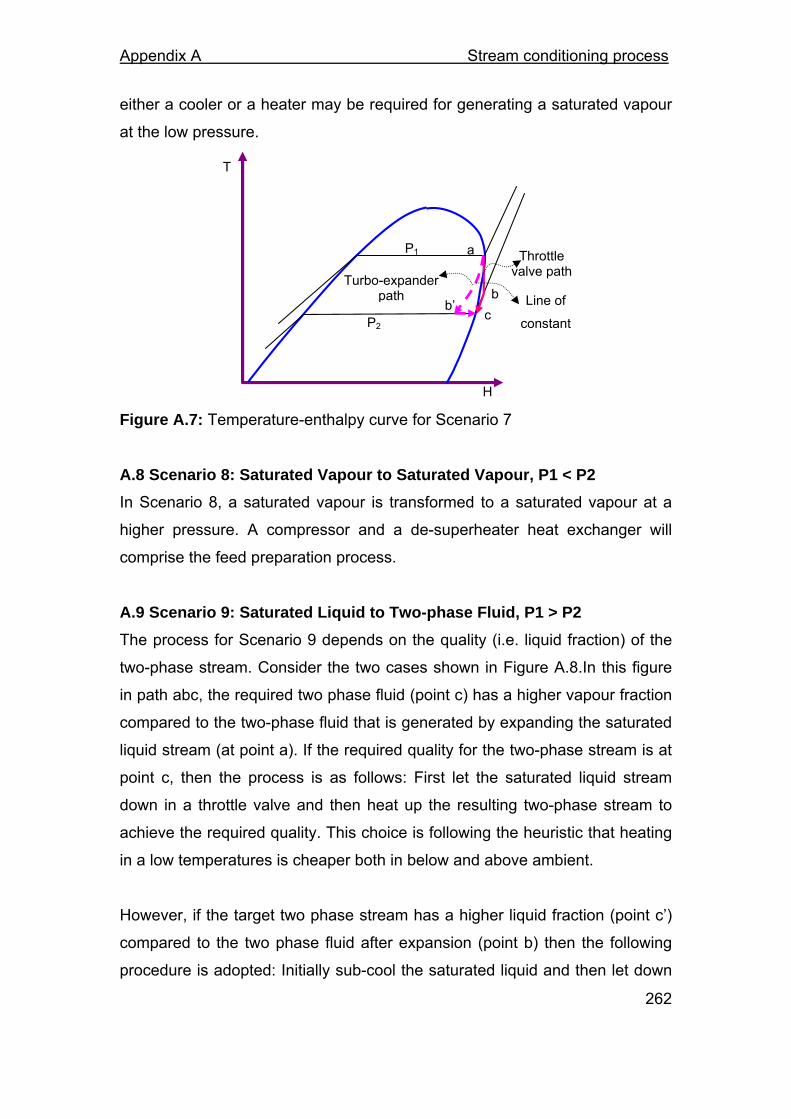
Appendix A Stream conditioning process
262
either a cooler or a heater may be required for generating a saturated vapour
at the low pressure.
Figure A.7: Temperature-enthalpy curve for Scenario 7
A.8 Scenario 8: Saturated Vapour to Saturated Vapour, P1 < P2 In Scenario 8, a saturated vapour is transformed to a saturated vapour at a
higher pressure. A compressor and a de-superheater heat exchanger will
comprise the feed preparation process.
A.9 Scenario 9: Saturated Liquid to Two-phase Fluid, P1 > P2 The process for Scenario 9 depends on the quality (i.e. liquid fraction) of the
two-phase stream. Consider the two cases shown in Figure A.8.In this figure
in path abc, the required two phase fluid (point c) has a higher vapour fraction
compared to the two-phase fluid that is generated by expanding the saturated
liquid stream (at point a). If the required quality for the two-phase stream is at
point c, then the process is as follows: First let the saturated liquid stream
down in a throttle valve and then heat up the resulting two-phase stream to
achieve the required quality. This choice is following the heuristic that heating
in a low temperatures is cheaper both in below and above ambient.
However, if the target two phase stream has a higher liquid fraction (point c’)
compared to the two phase fluid after expansion (point b) then the following
procedure is adopted: Initially sub-cool the saturated liquid and then let down
T
a
b c
H
P1
P2
b’
Throttle valve path Turbo-expander
path Line of
constant
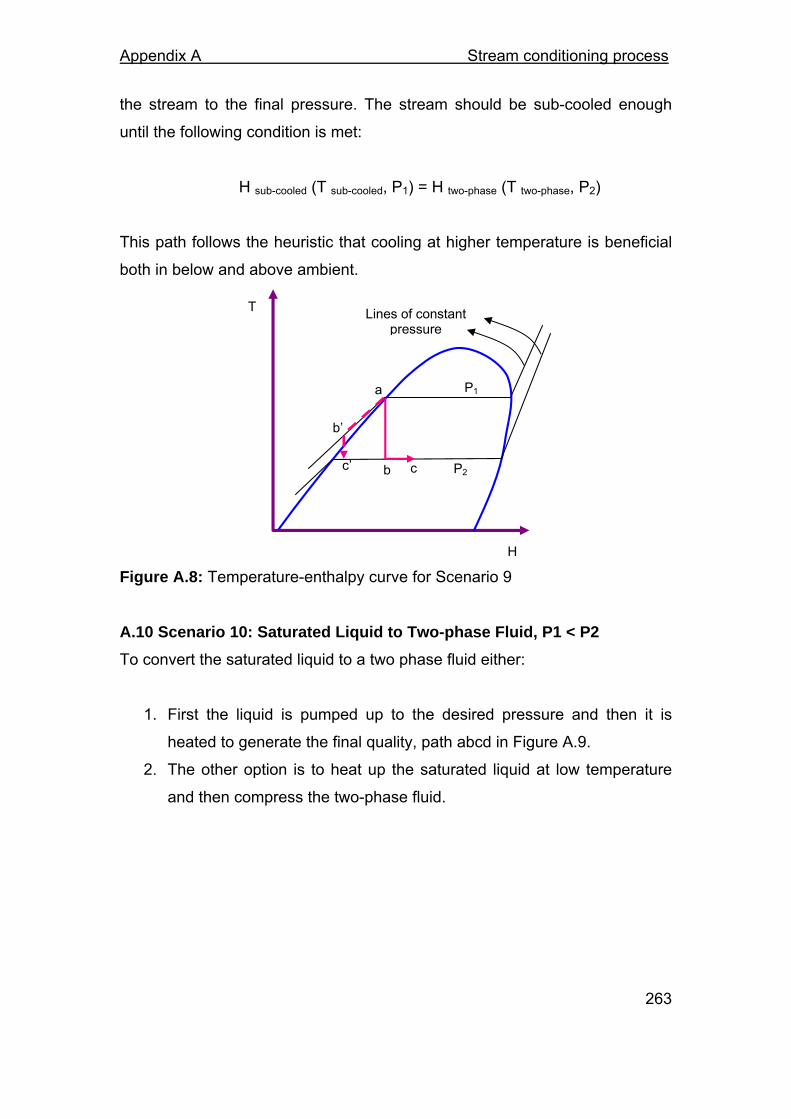
Appendix A Stream conditioning process
263
the stream to the final pressure. The stream should be sub-cooled enough
until the following condition is met:
H sub-cooled (T sub-cooled, P1) = H two-phase (T two-phase, P2)
This path follows the heuristic that cooling at higher temperature is beneficial
both in below and above ambient.
Figure A.8: Temperature-enthalpy curve for Scenario 9
A.10 Scenario 10: Saturated Liquid to Two-phase Fluid, P1 < P2 To convert the saturated liquid to a two phase fluid either:
1. First the liquid is pumped up to the desired pressure and then it is
heated to generate the final quality, path abcd in Figure A.9.
2. The other option is to heat up the saturated liquid at low temperature
and then compress the two-phase fluid.
a
b c
T
H
P1
P2
b’
c’
Lines of constant pressure
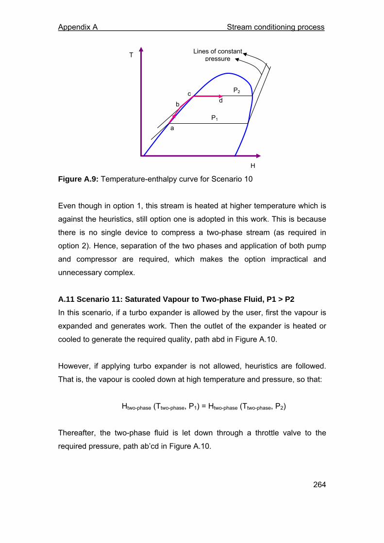
Appendix A Stream conditioning process
264
Figure A.9: Temperature-enthalpy curve for Scenario 10
Even though in option 1, this stream is heated at higher temperature which is
against the heuristics, still option one is adopted in this work. This is because
there is no single device to compress a two-phase stream (as required in
option 2). Hence, separation of the two phases and application of both pump
and compressor are required, which makes the option impractical and
unnecessary complex.
A.11 Scenario 11: Saturated Vapour to Two-phase Fluid, P1 > P2 In this scenario, if a turbo expander is allowed by the user, first the vapour is
expanded and generates work. Then the outlet of the expander is heated or
cooled to generate the required quality, path abd in Figure A.10.
However, if applying turbo expander is not allowed, heuristics are followed.
That is, the vapour is cooled down at high temperature and pressure, so that:
Htwo-phase (Ttwo-phase, P1) = Htwo-phase (Ttwo-phase, P2)
Thereafter, the two-phase fluid is let down through a throttle valve to the
required pressure, path ab’cd in Figure A.10.
a
b c
T
H
P1
P2
Lines of constant pressure
d
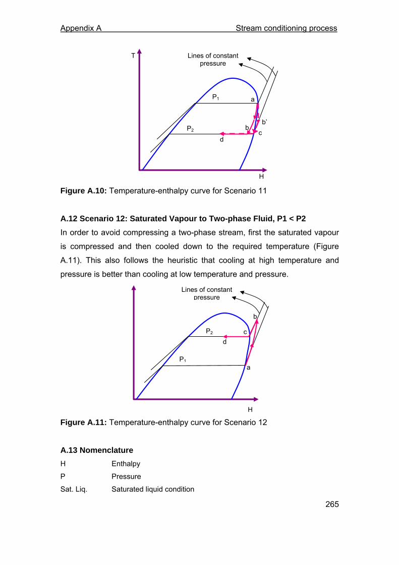
Appendix A Stream conditioning process
265
Figure A.10: Temperature-enthalpy curve for Scenario 11
A.12 Scenario 12: Saturated Vapour to Two-phase Fluid, P1 < P2 In order to avoid compressing a two-phase stream, first the saturated vapour
is compressed and then cooled down to the required temperature (Figure
A.11). This also follows the heuristic that cooling at high temperature and
pressure is better than cooling at low temperature and pressure.
Figure A.11: Temperature-enthalpy curve for Scenario 12
A.13 Nomenclature H Enthalpy
P Pressure
Sat. Liq. Saturated liquid condition
a
b
d
T
H
P1
P2
b’ c
Lines of constant pressure
a
b
c
H
P1
P2
Lines of constant pressure
d

Appendix A Stream conditioning process
266
Sat. Vap. Saturated vapour condition
T Temperature
Subscripts sub-cooled Sub-cooled condition
two-phase Two-phase condition
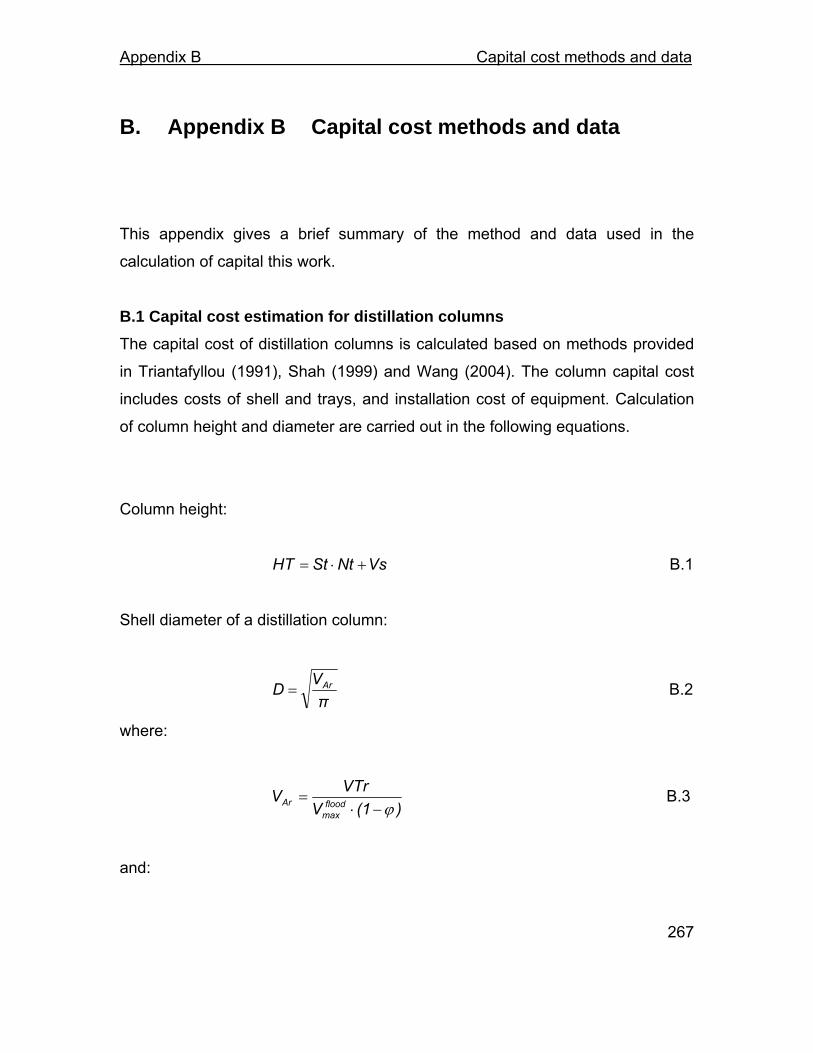
Appendix B Capital cost methods and data
267
B. Appendix B Capital cost methods and data
This appendix gives a brief summary of the method and data used in the
calculation of capital this work.
B.1 Capital cost estimation for distillation columns The capital cost of distillation columns is calculated based on methods provided
in Triantafyllou (1991), Shah (1999) and Wang (2004). The column capital cost
includes costs of shell and trays, and installation cost of equipment. Calculation
of column height and diameter are carried out in the following equations.
Column height:
VsNtStHT +⋅= B.1
Shell diameter of a distillation column:
πVD Ar= B.2
where:
)(1VVTrV flood
maxAr ϕ−⋅= B.3
and:

Appendix B Capital cost methods and data
268
vap
vapliq
sbflood
max ρρρCSV −
= B.4
The design pressure, column diameter and the height of the column are used to
determine the shell thickness and the weight of the column shell. The cost of the
column shell then predicted as a function of weight in tonnes using an equation
correlated from IChemE (2000). And and
⎥⎦
⎤⎢⎣
⎡+−
−−
= 11212
1shell y)y(y
)x(x)x(WWC B.5
where 2121 y ,y,x,x and are indices. Their values are given in table B.1.
The cost of a tray is a function of column diameter (D) and is predicted using the
following equation.
⎥⎦
⎤⎢⎣
⎡−
−⋅−+=
)x(xx(D)y(y
yNtC12
1)121tray B.6
Also, 2121 y ,y,x,x and are indices. Their values are given in Table B.2.
The column installation cost is predicted as a function of the column purchase
cost. The installation equation is also obtained from IChemE (2000), as in the
following equation.
installcolumnpurchase,columninstall, FCC ⋅= B.7
where column purchase cost is:
trayshellcolumnpurchase, CCC += B.8

Appendix B Capital cost methods and data
269
The installation factor is:
LGSBCEIIPErinstall FFFFFFFF ++++++= B.9
The values of various sub-factors in the installation cost can be obtained from
IChemE (2000).
B.2 Capital cost estimation for shell and tube heat exchangers The purchase cost of shell and tube heat exchangers, as given in Equation
(B10), is derived by Wang (2004) from the cost correlation graph in the IChemE
(2000).
510-46-
3-42STHEpurchase,
Ar104.095Ar101.027
-Ar109.013.0.32Ar-113.4Ar5391C
⋅⋅+⋅
⋅⋅++= (B.10)
where: Ar represents the area of the heat exchanger (m2) within a range of 10 to
1000m2. The installation cost of heat exchangers and the sub-factors of the
installation factors are the same as given in equations (B.7) and (B.9).
B.3 Capital cost of compressors The capital cost of centrifugal compressors in refrigeration processes is a
function of the power consumption, as expressed in Equation (B.11). This
equation is derived by Wang (2004) from graph 7.19 in IChemE (2000).
0.47
installcompressor )(Power)F68(1C += (B.11)
The installation factor Finstall can be calculated using Equation (B.9). Values of the
sub-factors can be found in IChemE (2000).

Appendix C Stream data for the case studies
270
C. Appendix C Stream data for the case studies
For feed and product coolers and heaters Table C.1: Case study BTEXC in section 5.6.2, Design I
1: stream name with respect to Figure 5.11; 2: negative numbers indicate to the enthalpy of hot stream. Table C.2: Case study BTEXC in section 5.6.2, Design II
1: stream name with respect to Figure 5.11; 2: negative numbers indicate to the enthalpy of hot stream.
Stream name1 Supply temperature
(˚C)
Target temperature
(˚C)
Enthalpy change2 (MW)
1 104 105 0.61
2 104 102 -1.4
3 141 158 2.6
4 114 159 3.4
5 80 50 -0.3
6 153 50 -1.4
7 181 50 -0.4
8 156 50 -1.3
9 169 50 -0.3
Stream name1 Supply temperature
(˚C)
Target temperature
(˚C)
Enthalpy change2 (MW)
1 104 107 1.7
2 104 104 -0.3
3 141 154 2.6
4 136 50 0.3
5 92 99 5
6 80 50 -2.6
7 111 50 -0.8
8 151 50 -1.3
9 164 50 -0.3
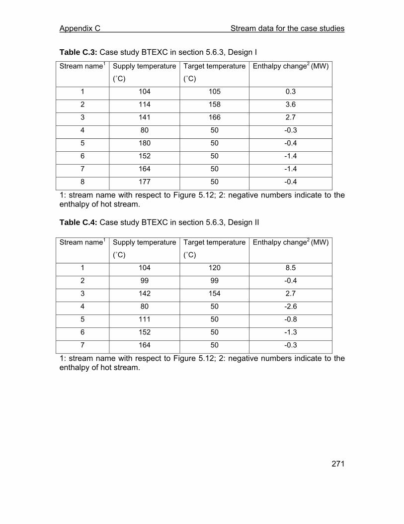
Appendix C Stream data for the case studies
271
Table C.3: Case study BTEXC in section 5.6.3, Design I
1: stream name with respect to Figure 5.12; 2: negative numbers indicate to the enthalpy of hot stream. Table C.4: Case study BTEXC in section 5.6.3, Design II
1: stream name with respect to Figure 5.12; 2: negative numbers indicate to the enthalpy of hot stream.
Stream name1 Supply temperature
(˚C)
Target temperature
(˚C)
Enthalpy change2 (MW)
1 104 105 0.3
2 114 158 3.6
3 141 166 2.7
4 80 50 -0.3
5 180 50 -0.4
6 152 50 -1.4
7 164 50 -1.4
8 177 50 -0.4
Stream name1 Supply temperature
(˚C)
Target temperature
(˚C)
Enthalpy change2 (MW)
1 104 120 8.5
2 99 99 -0.4
3 142 154 2.7
4 80 50 -2.6
5 111 50 -0.8
6 152 50 -1.3
7 164 50 -0.3
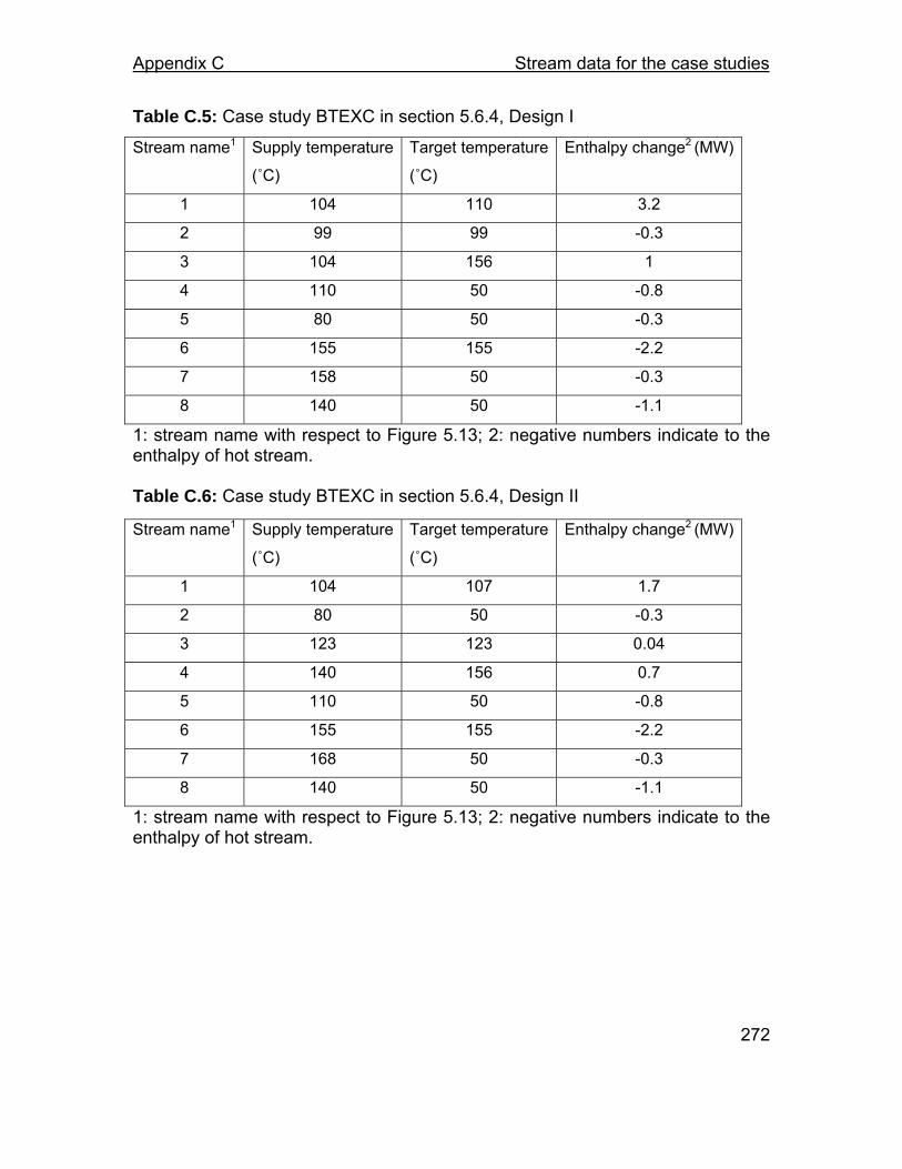
Appendix C Stream data for the case studies
272
Table C.5: Case study BTEXC in section 5.6.4, Design I
1: stream name with respect to Figure 5.13; 2: negative numbers indicate to the enthalpy of hot stream. Table C.6: Case study BTEXC in section 5.6.4, Design II
1: stream name with respect to Figure 5.13; 2: negative numbers indicate to the enthalpy of hot stream.
Stream name1 Supply temperature
(˚C)
Target temperature
(˚C)
Enthalpy change2 (MW)
1 104 110 3.2
2 99 99 -0.3
3 104 156 1
4 110 50 -0.8
5 80 50 -0.3
6 155 155 -2.2
7 158 50 -0.3
8 140 50 -1.1
Stream name1 Supply temperature
(˚C)
Target temperature
(˚C)
Enthalpy change2 (MW)
1 104 107 1.7
2 80 50 -0.3
3 123 123 0.04
4 140 156 0.7
5 110 50 -0.8
6 155 155 -2.2
7 168 50 -0.3
8 140 50 -1.1

Appendix C Stream data for the case studies
273
Table C.7: Case study BTEXC in section 5.6.5
1: stream name with respect to Figure 5.14; 2: negative numbers indicate to the enthalpy of hot stream. Table C.8: Case study LNG in section 7.2.2
1: stream name with respect to Figure 5.14; 2: negative numbers indicate to the enthalpy of hot stream. Table C.9: Case study LNG in section 7.3.2
1: stream name with respect to Figure 5.14; 2: negative numbers indicate to the enthalpy of hot stream.
Stream name1 Supply temperature
(˚C)
Target temperature
(˚C)
Enthalpy change2 (MW)
1 104 104 0.2
2 140 157 0.6
3 110 50 -0.8
4 80 50 -0.3
5 156 156 -2.6
6 169 50 0.3
7 140 50 -1.1
Stream name1 Supply temperature
(˚C)
Target temperature
(˚C)
Enthalpy change2 (MW)
1 -114 34 20.4
2 23 -24 -9.9
3 146 123 -2.9
Stream name1 Supply temperature
(˚C)
Target temperature
(˚C)
Enthalpy change2 (MW)
1 35 -17 -11.9
2 17 24 3.8
3 62 150 3.8
4 146 145 -1.2
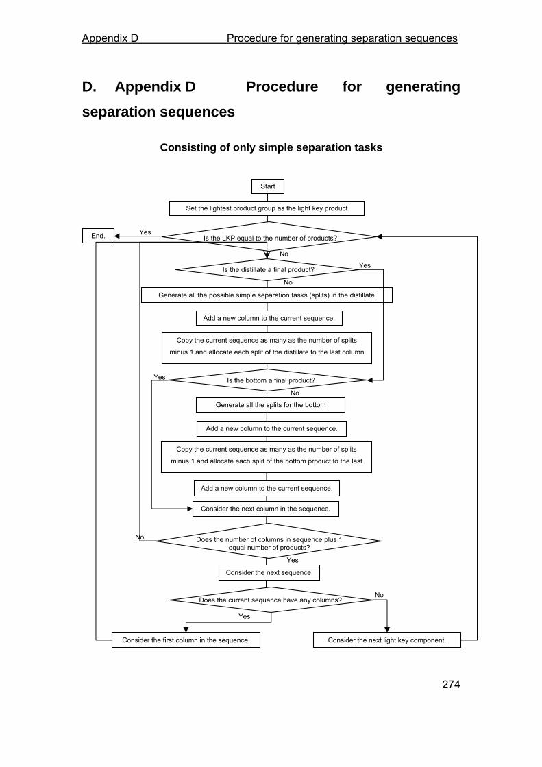
Appendix D Procedure for generating separation sequences
274
D. Appendix D Procedure for generating separation sequences
Consisting of only simple separation tasks
Start
Is the LKP equal to the number of products?
Is the distillate a final product?
Add a new column to the current sequence.
Generate all the possible simple separation tasks (splits) in the distillate
Add a new column to the current sequence.
Generate all the splits for the bottom
Yes
No
Yes
Yes
No
Yes
No
No
Yes
No
Copy the current sequence as many as the number of splits
minus 1 and allocate each split of the distillate to the last column
Is the bottom a final product?
Copy the current sequence as many as the number of splits
minus 1 and allocate each split of the bottom product to the last
Add a new column to the current sequence.
Consider the next column in the sequence.
Does the number of columns in sequence plus 1 equal number of products?
Set the lightest product group as the light key product
Consider the next sequence.
Does the current sequence have any columns?
Consider the first column in the sequence. Consider the next light key component.
End.