Departamento de Arquitectura, Construccion y Sistemas Oceanicos y Navales

Escuela Tecnica Superior Ingenieros Navales

Universidad Politecnica de Madrid

PhD Thesis

Design of a physical and interactive real-time

Simulator based on a dynamic VPP as a support

tool for sailing yacht design and operation

Ignacio Castaneda SabadellM. Sc. in Naval Architecture, Marine and Ocean Engineering

Supervisors:

Manuel Ruiz de Elvira

Ph.D. in Naval Architecture

Francisco Perez Arribas

Ph.D. in Naval Architecture

2018

“J’ecoute la mer, j’ecoute le vent, j’ecoute les voiles qui parlent avec la

pluie

et les etoiles dans les bruits de la mer et je n’ai pas sommeil.”

Bernard Moitessier

Acknowledgements

I would like to thank the following people for their assistance and support

during the PhD:

• To my supervisor Manuel Ruiz de Elvira for all the knowledge, ex-

perience, help, resources and support he brought to me constantly

during the whole process (from the first idea to the last word in the

text). He really helped me deeply understand how a sailing boat

works. Without his help, this work would not be possible.

• To my supervisor Francisco Perez Arribas for all the help and support

he brought to me during the development of the thesis and for all the

help and comments he gave me when teaching together in the UPM.

• To Prof. Ricardo Zamora, the person that introduced me to the

technical perspective of sailing yachts, allowing me to discover this

beautiful side of sailing.

• To Prof. Antonio Souto, for providing some of the resources needed

for the development of the thesis.

• To Mike and Caz Drummond, who proofread tirelessly the thesis to

the very last moment, helping me any time I needed and improving

the thesis quality thanks to their corrections, comments and sug-

gestions. I also need to thank Mike for sharing with me technical

comments and suggestions, helping me to understand a lot of differ-

ent aspects of this work.

• To Prof. Richard G.J. Flay and all the people working on the TFWT

of the University of Auckland for their warm welcome to the wind

tunnel and for sharing with me their knowledge on how sails and wind

tunnels work. The development of specific parts of this work would

not be possible without them. They also gave me the opportunity to

go to New Zealand and discover such an amazing place and people.

• To Andrew Mason who guided me when I was starting to work with

VR engines and helped me to understand and know the different

options available for the simulator.

• To Jose Luis Vela and Javier Cuevas who gave me ideas and advice on

how the simulator has to be developed and built, helping me discover

different strategies for the simulator implementation.

• To the former director of the CEHINAV, Prof. Luis Perez Rojas and

all the people working there, especially to Patricia Alcanda, Javier

Calderon, Elkin Botia and Jose Luis Cercos Pita, for all their help

and support, and for looking after me during the whole process.

• To my PhD colleagues from the University of Auckland for all the

help they brought to me and all the great moments we shared to-

gether during my research stay.

• To Benoit Marie for helping me to understand the Moth foiler sail-

boat and for sharing with me important information about it.

• To my group of friends of Devonport in Auckland, for their warm

welcome and the great times we shared together during my research

stay in New Zealand, becoming almost my family there when I was

far away from home.

• To my Hydraulink sailing friends, for letting me sailing and share

fun times with them, making my research stay more enjoyable and

interesting.

• To the international experts Richard Luco, Dan Walker and espe-

cially to Jerome H. Milgram, who reviewed the draft and provided

insightful comments and advice that improved the final version of

this work.

• A mis padres, hermana y amigos por aguantar mi trabajo y pre-

ocupaciones a lo largo de toda la tesis, dandome animos y apoyo.

Me gustarıa agradecer tambien a Ana, que me ha acompanado a lo

largo de todo este proceso, y a su familia por haberme aguantado y

ayudado durante la consecucion de este trabajo.

4

Abstract

Performance assessment and training are two major components in tech-

nified high-level sports. Recently, high-performance sailing competitions

have been forced to change with the use of the foiling technology and the

training restrictions, more often included within competition rules. To

answer those new situations, a new design and training tool has to be

developed. Up until now, the performance assessment was made calculat-

ing the balance of forces and moments using a Velocity Prediction Pro-

gram (VPP). This procedure was more than capable of dealing with con-

ventional displacement sailboats but the dynamic nature of foiling boats

compelled the development of a time-domain VPP for dynamic analysis

towards a better performance. In order to improve the dynamic analysis

capabilities of the VPP and to add the ability for it to be used for training,

a new tool is proposed to fulfil those requirements: the simulator.

Throughout this work the concept of the simulator has been discussed

identifying its fundamental components, namely:

• The time-domain VPP.

• The motion Platform.

• The visualization system.

• The physical user interface for the simulator operation.

The different uses and applicability for this concept are explored in order

to identify the potential benefits of such a tool in a high-performance

environment. The different components are analysed, identifying specific

problems in each area and proposing different solutions. All of this work

allows proposing a modular framework of a simulator to be used in high-

performance sailing boat design and training.

Resumen

La evaluacion del rendimiento y el entrenamiento son dos de los com-

ponentes principales en los deportes tecnificados de alto nivel. Reciente-

mente, las competiciones de vela de alto rendimiento se han visto obligadas

a cambiar con la aparicion y el uso de los “foils” y las restricciones de en-

trenamiento, incluidas mas a menudo dentro de las reglas de las competi-

ciones. Para responder a estas nuevas situaciones, se debe desarrollar una

nueva herramienta de diseno y entrenamiento. Hasta ahora, la evaluacion

del rendimiento en barcos de vela se realizaba calculando el equilibrio de

fuerzas y momentos utilizando un programa de prediccion de velocidad

(VPP). Este procedimiento es mas que capaz con veleros convencionales,

pero la naturaleza dinamica de los barcos con “foils” ha obligado al desar-

rollo del VPP en el dominio del tiempo para permitir el analisis dinamico

de este tipo de barcos en busca de un mayor rendimiento. Con el fin de

mejorar las capacidades de analisis dinamico del VPP y agregar la ca-

pacidad de ser utilizado durante el entrenamiento, se propone una nueva

herramienta que cumple con esos requisitos: el simulador.

A lo largo de este trabajo, se ha discutido el concepto del simulador iden-

tificando sus componentes fundamentales, a saber:

• El VPP en el dominio del tiempo.

• La plataforma de movimiento.

• El sistema de visualizacion.

• La interfaz de usuario fısica para la operacion del simulador.

Se exploran los diferentes usos y la aplicabilidad de este concepto para

identificar los beneficios potenciales de una herramienta de este tipo en

un entorno de alto rendimiento. Los diferentes componentes son anal-

izados, identificando problemas especıficos en cada area y proponiendo

diferentes soluciones. Todo este trabajo permite proponer un simulador

como entorno modular para ser utilizado en el diseno y entrenamiento en

competiciones de vela de alto rendimiento.

7

Contents

Glossary 2

1 Overview 4

1.1 Background and Context . . . . . . . . . . . . . . . . . . . . . . . . . 4

1.2 The Simulator: A Definition . . . . . . . . . . . . . . . . . . . . . . . 5

1.3 State-of-the-Art . . . . . . . . . . . . . . . . . . . . . . . . . . . . . . 6

1.4 Contributions . . . . . . . . . . . . . . . . . . . . . . . . . . . . . . . 9

1.5 Outline of the Thesis . . . . . . . . . . . . . . . . . . . . . . . . . . . 10

2 The Sailing Yacht Simulator 12

2.1 A New Design Asset . . . . . . . . . . . . . . . . . . . . . . . . . . . 13

2.1.1 Advanced Performance Assessment . . . . . . . . . . . . . . . 13

2.1.2 Early Testing of Design Features . . . . . . . . . . . . . . . . 13

2.1.3 Assistance to Energy Management . . . . . . . . . . . . . . . 14

2.1.4 Continuous Dynamic VPP Verification . . . . . . . . . . . . . 14

2.1.5 Two Boat Performance Evaluation with Only One Real Boat . 14

2.2 The Perfect Testing Platform . . . . . . . . . . . . . . . . . . . . . . 15

2.2.1 No Dependency on Weather Conditions . . . . . . . . . . . . . 15

2.2.2 Evaluate Safety Limits and Corrections . . . . . . . . . . . . . 15

2.2.3 Evaluation of Optimal Response to Soft Transitions and Pat-

terns of Changes . . . . . . . . . . . . . . . . . . . . . . . . . 15

2.2.4 Evaluation of Situations with Similar Performances but Differ-

ent Executions . . . . . . . . . . . . . . . . . . . . . . . . . . 16

2.2.5 Evaluate Early Signs for Required Corrections . . . . . . . . . 16

2.2.6 Test Deck Gear . . . . . . . . . . . . . . . . . . . . . . . . . . 16

2.2.7 Provide a Test Platform for Augmented Reality . . . . . . . . 17

2.3 A New Interface for Improved Communications Between Athletes and

Designers . . . . . . . . . . . . . . . . . . . . . . . . . . . . . . . . . 18

i

2.4 A Sailor’s Training Tool . . . . . . . . . . . . . . . . . . . . . . . . . 19

2.4.1 Assistance Towards a Steeper Learning Curve . . . . . . . . . 19

2.4.2 Training for Subsequent On-The-Water Tests . . . . . . . . . 19

2.4.3 Race Preparation . . . . . . . . . . . . . . . . . . . . . . . . . 20

2.4.4 Model Racing Situations . . . . . . . . . . . . . . . . . . . . . 20

2.4.5 Training of Natural Reactions . . . . . . . . . . . . . . . . . . 21

2.4.6 Training Anticipation Regarding what to Expect from Unusual

Situations . . . . . . . . . . . . . . . . . . . . . . . . . . . . . 21

2.4.7 Anticipate the Behaviour of a New Design or Type of Yacht . 21

2.4.8 Virtual Repetition of Real On-The-Water Training and Regattas 22

2.5 A Modular Approach of the Sailing Yacht Simulator . . . . . . . . . . 22

2.6 The Concepts of Immersion, Presence and Fidelity . . . . . . . . . . . 24

3 PASim, the Simulator Core 26

3.1 The VPP as the Heart of a 6-DOF Sailing Simulator . . . . . . . . . 26

3.2 From a Static Equilibrium to a Time-Domain Calculation . . . . . . . 27

3.3 Physical Models for Forces and Moments . . . . . . . . . . . . . . . . 30

3.3.1 Interpolated Models . . . . . . . . . . . . . . . . . . . . . . . 31

3.3.1.1 Experimental Data . . . . . . . . . . . . . . . . . . . 32

3.3.1.2 Numerical Data . . . . . . . . . . . . . . . . . . . . . 36

3.3.1.3 Special Considerations . . . . . . . . . . . . . . . . . 39

3.3.2 Analytical Models . . . . . . . . . . . . . . . . . . . . . . . . . 40

3.3.2.1 Analytical Models . . . . . . . . . . . . . . . . . . . 41

3.3.2.2 Numerical Methods Solved in Execution Time . . . . 42

3.3.2.3 Numerical Methods Combined with Interpolation Schemes 44

3.3.2.4 Unsteady Model Correction . . . . . . . . . . . . . . 45

3.3.3 Other Models . . . . . . . . . . . . . . . . . . . . . . . . . . . 47

3.4 Time-Domain Solver Numerical Schemes . . . . . . . . . . . . . . . . 48

3.5 Autopilots . . . . . . . . . . . . . . . . . . . . . . . . . . . . . . . . . 53

3.5.1 Boat Elements . . . . . . . . . . . . . . . . . . . . . . . . . . 55

3.5.2 Algorithms . . . . . . . . . . . . . . . . . . . . . . . . . . . . 57

3.5.3 A General Approach for Neural-Network-Based Autopilots . . 59

3.5.4 The Simulator as a Safe Test Environment for Control Systems 59

3.5.5 Use of Autopilots to Improve Performance . . . . . . . . . . . 60

3.5.6 Unstable Boats . . . . . . . . . . . . . . . . . . . . . . . . . . 60

ii

3.6 A Note on Multi-Threading Execution and Multi-Computer Configu-

ration . . . . . . . . . . . . . . . . . . . . . . . . . . . . . . . . . . . 63

3.7 An Example : The Moth Foiler . . . . . . . . . . . . . . . . . . . . . 65

3.7.1 The Boat . . . . . . . . . . . . . . . . . . . . . . . . . . . . . 66

3.7.2 Forces and Moments Models . . . . . . . . . . . . . . . . . . . 67

3.7.3 An Example of the Foiling Moth Simulator Usage: The Tran-

sition Study From Non-Foiling to Foiling . . . . . . . . . . . . 70

4 The Motion Platform 73

4.1 The Degrees of Freedom . . . . . . . . . . . . . . . . . . . . . . . . . 74

4.1.1 Conventional Monohulls and Slow Multihulls . . . . . . . . . . 74

4.1.2 Fast Multihulls and Foiling Boats . . . . . . . . . . . . . . . . 75

4.2 Reproduction of Motion and Position Versus Reproduction of Rota-

tional Velocities and Linear Accelerations . . . . . . . . . . . . . . . . 76

4.2.1 A Tool to Reproduce Motions and Position . . . . . . . . . . . 77

4.2.2 A Tool to Reproduce Rotational Velocities and Linear Acceler-

ations . . . . . . . . . . . . . . . . . . . . . . . . . . . . . . . 78

4.3 The Stewart Platform: A Six Degrees of Freedom Parallel Robot . . . 80

4.3.1 Description . . . . . . . . . . . . . . . . . . . . . . . . . . . . 81

4.3.2 Motion Cue Generation and Analysis Algorithms . . . . . . . 82

4.3.2.1 Inverse Kinematics . . . . . . . . . . . . . . . . . . . 83

4.3.2.2 Direct Kinematics . . . . . . . . . . . . . . . . . . . 84

4.3.2.3 Inverse Dynamics . . . . . . . . . . . . . . . . . . . . 84

4.3.3 Limitations . . . . . . . . . . . . . . . . . . . . . . . . . . . . 86

4.4 Washout Algorithm . . . . . . . . . . . . . . . . . . . . . . . . . . . . 87

4.4.1 General Description . . . . . . . . . . . . . . . . . . . . . . . . 87

4.4.1.1 Classical Washout . . . . . . . . . . . . . . . . . . . 87

4.4.1.2 Optimal Washout . . . . . . . . . . . . . . . . . . . . 90

4.4.1.3 Adaptive Washout . . . . . . . . . . . . . . . . . . . 92

4.4.1.4 Notes on the Implementation . . . . . . . . . . . . . 94

4.4.2 Washout Algorithm Tuning . . . . . . . . . . . . . . . . . . . 95

4.4.2.1 Vestibular Model . . . . . . . . . . . . . . . . . . . . 95

4.4.2.2 Genetic Algorithms . . . . . . . . . . . . . . . . . . . 97

4.4.2.3 Time History Information Generation for Coefficients

Training . . . . . . . . . . . . . . . . . . . . . . . . . 98

iii

4.4.2.4 Filtering Parameter Selection Using a Vestibular Model

and Genetic Algorithms Training . . . . . . . . . . . 100

5 Visualisation Interface 103

5.1 Vision as the Main Source for Motion Simulation . . . . . . . . . . . 103

5.2 The Virtual Reality Engine to Represent the Optic Flow . . . . . . . 105

5.2.1 Simulator Needs . . . . . . . . . . . . . . . . . . . . . . . . . . 105

5.2.2 A Tool to Generate Environmental Cues . . . . . . . . . . . . 108

5.2.3 A Tool to Show Vital Information . . . . . . . . . . . . . . . . 112

5.2.4 A Tool that Improves Two Boat Interaction Awareness . . . . 114

5.3 Specific Challenges of a Realistic Visual Experience . . . . . . . . . . 115

5.4 Virtual Reality Representation Systems . . . . . . . . . . . . . . . . . 119

6 The Physical User Interface 122

6.1 A User Interface to Allow the Simulator Operation . . . . . . . . . . 122

6.2 From a Simple Control to a More Realistic Experience . . . . . . . . 123

6.2.1 Steering Elements . . . . . . . . . . . . . . . . . . . . . . . . . 125

6.2.2 Sails Operation . . . . . . . . . . . . . . . . . . . . . . . . . . 126

6.2.3 User Position . . . . . . . . . . . . . . . . . . . . . . . . . . . 127

6.2.4 New Interface Systems and Other Settings Adjustment . . . . 128

6.2.5 Cockpit Reproduction . . . . . . . . . . . . . . . . . . . . . . 129

7 Conclusions 130

A AC72 Dynamic Data Time History Plots 135

A.1 Time History Comparison for Different Numerical Schemes . . . . . . 136

A.2 Time History Comparison Using Euler and Midpoint Methods with

Different Time Steps . . . . . . . . . . . . . . . . . . . . . . . . . . . 144

B Time History Data of the Simulated Foiling Moth Runs 152

B.1 Time History Data of the Simulated Foiling Moth Run Using a Heel

PID Controller . . . . . . . . . . . . . . . . . . . . . . . . . . . . . . 152

B.2 Time History Data of the Simulated Foiling Moth Transition Run . . 158

C Multi-Threading Tests Time Results 165

iv

D Moth Foiler Models 169

D.1 Aerodynamic Models . . . . . . . . . . . . . . . . . . . . . . . . . . . 169

D.1.1 Sails . . . . . . . . . . . . . . . . . . . . . . . . . . . . . . . . 169

D.1.2 Windage . . . . . . . . . . . . . . . . . . . . . . . . . . . . . . 171

D.2 Hydrodynamic Models . . . . . . . . . . . . . . . . . . . . . . . . . . 171

D.2.1 Lifting Surfaces . . . . . . . . . . . . . . . . . . . . . . . . . . 171

D.2.2 Hull . . . . . . . . . . . . . . . . . . . . . . . . . . . . . . . . 173

D.3 Other Models . . . . . . . . . . . . . . . . . . . . . . . . . . . . . . . 174

D.3.1 Control Models . . . . . . . . . . . . . . . . . . . . . . . . . . 174

D.3.2 Other Hydrostatics and Weight Stability Models . . . . . . . . 174

E Washout Tuning Algorithm Results 176

Bibliography 181

v

List of Figures

2.1 Simulator general diagram of the modular implementation. . . . . . . 24

3.1 CEHINAV Towing Tank Facility in the ETSIN-UPM in Madrid. Pho-

tograph by CEHINAV Research Group . . . . . . . . . . . . . . . . . 33

3.2 Twisted Flow Wind Tunnel of the University of Auckland . . . . . . . 35

3.3 Flat plate effective AoA under the influence of a sinusoidal oscillation

followed by suddenly fixing the value of the angle of attack . . . . . . 46

3.4 Moth Foiler Wand Control System Explanation . . . . . . . . . . . . 47

3.5 AC72 boat speed time history for the different numerical schemes . . 50

3.6 AC72 pitch and sinkage time history comparison using Euler and Mid-

point methods . . . . . . . . . . . . . . . . . . . . . . . . . . . . . . . 51

3.7 AC72 boat speed time history comparison using Euler and Midpoint

methods with different time steps . . . . . . . . . . . . . . . . . . . . 52

3.8 Moth sailing in foiling mode. Photograph by Manuel Ruiz de Elvira . 66

3.9 Moth polar curve generated using PASim. . . . . . . . . . . . . . . . 70

3.10 BSP time history of the Moth foiling transition. . . . . . . . . . . . . 72

3.11 Sink time history of the Moth foiling transition. . . . . . . . . . . . . 72

4.1 Motion platform module block diagram . . . . . . . . . . . . . . . . . 74

4.2 49er dinghy sailing. Photograph by local Geelong yachtsman. Source:

https://commons.wikimedia.org/wiki/File:49er_skiff_sailing_

AUS_nationals_Geelong.jpg . . . . . . . . . . . . . . . . . . . . . . 75

4.3 AC50 (a) and AC45 (b) sailing. Photographs by Manuel Ruiz de Elvira 76

4.4 6-SPS (a) and 6-UPS (b) platforms . . . . . . . . . . . . . . . . . . . 81

4.5 Block diagram of the Inverse Kinematics implementation. . . . . . . . 83

4.6 Block diagram of the Inverse Dynamics implementation. . . . . . . . 86

4.7 Original flowchart of the Classical Washout implementation. Source:

Reid et al., Figure 14.1 in [151] . . . . . . . . . . . . . . . . . . . . . 89

vi

4.8 Original flowchart of the Optimal Washout implementation. Source:

Reid et al., Figure 14.2 in [151] . . . . . . . . . . . . . . . . . . . . . 92

4.9 Original flowchart of the Adaptive Washout implementation. Source:

Reid et al., Figure 14.3 in [151] . . . . . . . . . . . . . . . . . . . . . 93

5.1 VR engine module block diagram . . . . . . . . . . . . . . . . . . . . 108

5.2 Beaufort 4 (a) and Beaufort 8 (b) sea states generated with Unigine . 112

5.3 Basic way to show data for training and designing purposes using Unigine114

5.4 Moth foiler Scaled model with V-SPARs in the Twisted Flow Wind

Tunnel of the University of Auckland . . . . . . . . . . . . . . . . . . 116

5.5 V-SPARS processed image (a) and preliminary three-dimensional (b)

of a V-SPARS analysis for the Moth mainsail in a twisted flow at 45

degrees of AWA . . . . . . . . . . . . . . . . . . . . . . . . . . . . . . 117

5.6 Wool telltales . . . . . . . . . . . . . . . . . . . . . . . . . . . . . . . 119

6.1 Occulus Rift Touch hand-held controller. Photograph by Evan Amos.

Source: https://upload.wikimedia.org/wikipedia/commons/d/d8/

Oculus-Rift-Touch-Controllers-Pair.jpg . . . . . . . . . . . . . 124

6.2 Brushless electric motor with controller and integrated angular encoder 126

A.1 Time history comparison for different numerical schemes - BSP . . . 137

A.2 Time history comparison for different numerical schemes - Heel . . . . 138

A.3 Time history comparison for different numerical schemes - Pitch . . . 139

A.4 Time history comparison for different numerical schemes - Yaw . . . . 140

A.5 Time history comparison for different numerical schemes - Sinkage . . 141

A.6 Time history comparison for different numerical schemes - AWS . . . 142

A.7 Time history comparison for different numerical schemes - AWA . . . 143

A.8 Time history comparison using Euler and Midpoint methods with dif-

ferent time steps - BSP . . . . . . . . . . . . . . . . . . . . . . . . . . 145

A.9 Time history comparison using Euler and Midpoint methods with dif-

ferent time steps - Heel . . . . . . . . . . . . . . . . . . . . . . . . . . 146

A.10 Time history comparison using Euler and Midpoint methods with dif-

ferent time steps - Pitch . . . . . . . . . . . . . . . . . . . . . . . . . 147

A.11 Time history comparison using Euler and Midpoint methods with dif-

ferent time steps - Yaw . . . . . . . . . . . . . . . . . . . . . . . . . . 148

A.12 Time history comparison using Euler and Midpoint methods with dif-

ferent time steps - Sinkage . . . . . . . . . . . . . . . . . . . . . . . . 149

vii

A.13 Time history comparison using Euler and Midpoint methods with dif-

ferent time steps - AWS . . . . . . . . . . . . . . . . . . . . . . . . . 150

A.14 Time history comparison using Euler and Midpoint methods with dif-

ferent time steps - AWA . . . . . . . . . . . . . . . . . . . . . . . . . 151

D.1 Setup used in the TWFT for Moth aerodynamic model measurements 170

viii

List of Tables

4.1 Cumulated linear sensed error for the Classical Washout . . . . . . . 90

4.2 Cumulated linear sensed error for the Adaptive Washout . . . . . . . 94

B.1 Time history of the simulated foiling Moth run using a heel PID controller153

B.2 Detailed last 4 seconds of the simulated foiling moth run using a heel

PID controller . . . . . . . . . . . . . . . . . . . . . . . . . . . . . . . 155

B.3 Time History of the Simulated Foiling Moth Transition Run . . . . . 159

B.4 Kinematic cues of the first four seconds of the Foiling Moth Transition

Run Using Classical Washout . . . . . . . . . . . . . . . . . . . . . . 161

B.5 Kinematic cues of the first four seconds of the Foiling Moth Transition

Run Using Adaptive Washout . . . . . . . . . . . . . . . . . . . . . . 163

C.1 Multi-threading tests time results using Moth Foiler models . . . . . 165

E.1 NSGAII algorithm results . . . . . . . . . . . . . . . . . . . . . . . . 177

E.2 MOEA/D algorithm results . . . . . . . . . . . . . . . . . . . . . . . 178

E.3 NSGAIII (outer dimension reference point generation only) algorithm

results . . . . . . . . . . . . . . . . . . . . . . . . . . . . . . . . . . . 179

E.4 NSGAIII (inner and outer dimension reference point generation) algo-

rithm results . . . . . . . . . . . . . . . . . . . . . . . . . . . . . . . . 180

ix

1

Glossary

The following glossary of the different sailing terms used throughout this work is

provided for a better understanding of the text.

Angle of Attack (AoA): angle between a reference line of a body travelling through

a fluid and the velocity vector of such a fluid.

Apparent Wind Angle (AWA): angle between the apparent wind vector and the

boat centre line.

Apparent Wind Speed (AWS): magnitude of the apparent wind vector.

Apparent Wind: wind vector resulting from the combination of the true wind vec-

tor in which the boat is sailing and the negative of the boat speed vector.

Cant: angle of rotation on the local X-axis (approximately horizontal and longitu-

dinal to the sailboat) of the different movable elements on-board.

Cunningham: downhaul found on Bermuda rigged sailboat attached to the tack of

the mainsail.

Daggerboard: vertically moving vertical lifting surface used to generate the hydro-

dynamic lateral force to compensate the aerodynamic one.

Downhaul: trimming line allowing the application of a downward force on the luff

of a sail.

Genoa: larger headsail that overlaps the mainsail.

Heel: angle of rotation on the X-axis of the sailboat.

Keel: fixed vertical lifting surface used to generate the hydrodynamic lateral force

to compensate the aerodynamic one.

2

Leech: the trailing edge of a sail.

Luff: the leading edge of a sail.

Mainsheet: trimming line attached to the boom principally allowing control of the

mainsail position (in and out) by controlling the leech tension.

Offshore Racing Council (ORC): international body in charge of establishing

and maintaining a series of competitive rules for offshore handicap sailing boat

racing.

Outhaul: trimming line attached to the sail clew allowing for control of the shape

of the foot of the sail.

Pitch: angle of rotation on the Y-axis of the sailboat.

Race Modelling Program (RMP): software that models the race, using VPP

and weather data, between different contenders to estimate a win or loss prob-

ability for each one of them.

Rake: angle of rotation on the local Y-axis (approximately horizontal and transversal

to the sailboat) of the different movable elements on-board.

Rudder: rotating vertical lifting surface normally located near the transom of the

sailboat used for steering.

Toe: angle of rotation on the local Z-axis (approximately vertical to the sailboat) of

the different movable elements on-board.

Traveller: trimming device normally consisting of a line and a track allowing the

control of the boom position maintaining the mainsheet tension.

Velocity Made Good (VMG): speed of the sailing boat towards a certain target

or destination (normally referred to a windward or leeward position and thus

becoming the projection of the boat speed along the wind direction). Normally,

it is different from the boat speed unless the boat is sailing directly towards

such target or destination.

Yaw: angle of rotation on the Z-axis of the sailboat.

3

Chapter 1

Overview

1.1 Background and Context

The America’s Cup represents the pinnacle of sailing sport and has become one the

principal exponents of how advanced technology and sports can work hand in hand.

This assimilation has ensured that the competing boats of today are not simple sail-

boats anymore but complex machines with a huge number of setups and handling

possibilities. Being able to understand the boat’s behaviour and handling, and being

able to find the best setup regarding the boat settings and the design parameters,

lead the teams to achieve a better performance.

Until now, the main tool for the sail boat design team was the Velocity Prediction

Program or VPP. This software is able to solve the boat equilibrium of forces up to the

six degrees of freedom (DOF) of a rigid solid body. The information obtained after the

equilibrium is solved (static approach) is the boat speed and the boat sailing attitude;

the main elements characterising the boat performance. With the appearance of

vertically lifting hydrofoils in the world of sailing, the need for new performance

assessment tools became more and more obvious. The information generated by a

traditional Velocity Prediction Program is no longer enough to understand the boat

behaviour. Because of the dynamic nature of the foiling yacht, it is important to

also know how the boat accelerates, the stability and how the boat handles. A new

approach has appeared allowing us to obtain all the information needed. Instead of

facing the problem as a static one based on the force and moments equilibrium, this

new approach consists of solving the equations of the dynamics of the rigid body

in the time domain. This is the reason for the appearance of the dynamic Velocity

Prediction Program (VPP). The main problem now is to find a way to be able to

interpret all this information in the manner that allows the designer and the user to

understand how the boat behaves, and then apply all that knowledge to improve the

4

boat design and the crew boat-handling abilities. New forms of representation and

interaction are needed and a new layer of complexity has to be implemented over the

dynamic VPP leading to the development of the physical sailing boat simulator.

1.2 The Simulator: A Definition

According to Manuel Ruiz de Elvira’s PhD Thesis [156] the simulator must provide

enough information for the user, the sailor, to generate the best user experience, as

close as possible to the reality. The simulator has to be able to also accept inputs

from the user in the same way a sailor interacts with an actual boat. In summary,

it is a two-way relationship that allows the user to feel he is actually sailing a real

sailboat. To be able to achieve that, some of the sailor’s senses must be stimulated

in the same way they would be on a real boat. For instance, the simulator has to

reproduce, allow or provide:

• The boat accelerations.

• The visual surroundings of the moving boat.

• Any data available on-board about the external conditions affecting the boat,

including wind parameters, VMG...

• The way to interact with the boat elements such as rudder tiller, sail trimming

controls...

The main objective when developing such a tool is to find the way to accomplish

these requirements. From the technical point of view, the simulator is then the sum

of a number of elements working together to produce the result needed. For instance:

• A time-domain dynamic VPP, which brings together all the models describing

the physical reality of the boat and capable of calculating the yacht behaviour

based on different environmental and user inputs.

• A parallel robot or moving platform being able to reproduce the boat accelera-

tions.

• A Virtual Reality (VR) interface like a VR headset to reproduce, in an immer-

sive way, all the visual environment related to a moving yacht.

• A physical user interface that allows the sailor to handle and adjust the virtual

sailboat the same way as he usually would in a real one.

5

These four elements represent the essential ones that the simulator needs to give

the best experience. Without them it is not possible to offer a virtual sailing expe-

rience as close as possible to the reality, knowing that a perfect match in the user

sensations is impossible. Other elements could also be integrated such as a Race

Modelling Program (RMP) to model actual racing situations with other competitors.

The goal is then to have an experience that could help the sailing team and the design

team to improve their handling skills and the overall performance of the boat.

1.3 State-of-the-Art

In such a competitive world, any advantage can be the key to beat your rival so

having the access to such a tool can make all the difference. Surprisingly, any of the

attempts to develop such tools were partially unsuccessful in the past. All the efforts

seemed to head in a different direction, such as, a tool to teach how to sail or to

evaluate physical performance of the crew.

The first attempts to simulate a sailing boat were carried out in 1965 by Hansen

[73] with his “Sailing Simulator” patent, later Waddington et al. [181] in 1971

presented their “Simulating apparatus for teaching the art of sailing” and in 1976

Nishimura and Kaoru [123] also presented their patent of a “Sailing Simulator”.

In the late 1980’s and early 1990’s two simulators were developed by Harrison ([24],

[111]) and Blackburn ([16], [17]) to study the physiology of hiking in a dinghy in a

controlled environment. Harrison’s simulator consisted of a rotating, one degree of

freedom, Europe dinghy deck molding, moved with a weight system and using pumped

water to simulate the heeling moment, and completed with a primitive graphical and

control interface. Blackburn’s simulator was composed of an Olympic Laser Class

dinghy mounted on a fixed frame to allow them to measure the hiking moment. A

video of actual Laser sailing was projected using a television screen to allow the

sailor to mimic the movements on the video being shown. This concept of using the

simulator as a laboratory tool was used more recently by Cunningham and Hale in

2007 [37].

With the efforts heading in other directions, in 1994, Kibuchi et al.[93] developed

a sail training simulator focused on the teaching of sailing instead of physiological

research. It was formed by using a single-handed sailboat with pneumatic rams to

control the boat’s roll motion and the boom and rudder moment feedback. It was

completed by two computer graphics displays, one in the bow and another in the

6

stern. To reproduce the manoeuvring characteristics of the boat, a mathematical

model was implemented.

Based on Harrison’s simulator, in 1994 Walls and Saunders [184] developed an

Olympic Laser class dinghy simulator. It consisted of a deck molding of the boat

supported by a steel frame, using a computer-controlled weight system to reproduce

the heeling moment. The device was completed by a trimming and steering mecha-

nism and a computer display. In order to obtain a more realistic experience, Gale and

Walls improved this design incorporating new elements as is presented in [62]. Such

elements were a mathematical model of the boat dynamics, a new motion control

system based on pneumatic rams and an improved 3D graphics visual system with

audio feedback. The dinghy deck was mounted on a pivoting support frame and had

the ability to be changed in order to simulate different classes of boats. The boat

motion was driven by a pneumatic ram counteracting the righting moment of the

hiking sailor. Another pneumatic ram was connected to the rudder tiller to simulate

the rudder moment. It was completed by a spring system reproducing the mainsheet

tension. To improve the sensation of reality, some elements of the deck gear were

positioned in their real position (original mainsheet blocks and tiller). Finally, the

3D graphics visual system was able to reproduce different elements such as hull, rig

and water, including shading for the wind gusts, and different floating elements. The

main goal of all this work as described in [62] was to obtain a simulator that in com-

parison to a real dinghy “should have had similar appearance and dynamic response,

elicit similar posture, body movement and decision making processes from the sailor,

give appropriate sensory feedback and provide appropriate decision making cues”.

The increased capabilities of this simulator allowed Walls et al. [183] to carry-out the

performance assessment of different sailors in upwind dinghy-sailing conditions.

All this effort made by Gale and Walls lead to the development of the first com-

mercial sailing boat simulator, the Virtual Sailing VS-1 described by Binns, Bethwaite

and Saunders in [12]. Some changes were made over the original simulator; for in-

stance, a full dinghy suspended on rollers was used to obtain a more realistic feel

of the boat and the roll angle. A new pneumatic system was adopted with higher

pneumatic capabilities allowing a faster and more powerful response. The physical

model of the boat was also changed, this time using some basic VPP or velocity

prediction program techniques and new physical models. The original system based

on three degrees of freedom (forward force balance, heel moment balance and yaw

moment balance) was replaced with a four degrees of freedom model, adding side

force balance.

7

Since then, the simulators created by Virtual Sailing were used in different areas.

In [115] Mooney et al. present several different uses:

• Olympic sail training.

• Engineering education.

• Disabled sail training.

• Instruction for novice sailors.

In 2012, a Simulation Verification, Validation and Calibration (VVC) of the Vir-

tual Sailing simulators was conducted by Binns et al. [13]. On-water measurements of

different manoeuvres were taken with a specially developed data acquisition system.

The same procedure was made with the simulator, repeating the same manoeuvres

and collecting the same data. All the data was then compared to show a good correla-

tion between sailing times measured on-water and those obtained with the simulator.

Some problems regarding the fidelity of the rudder force feedback system appeared.

Further work regarding the effect of motion on presence for a sailing simulator was

performed by Mulder and Verlinden in [117] and [116]. They developed a system with

a dinghy hull mounted on top of a Stewart platform1 with the visualisation system

mounted outside the platform. The goal was to evaluate the feedback of five sailors

to roll, pitch and heave displacement during the simulation with the possibility of

adjusting the parameters controlling the amount of movement in different runs. The

results showed that the most engaging motion to contribute the sense of presence

was the roll motion. Pitch motion was considered of less importance except when

combined with roll motion, improving the sense of presence. The authors consider

that heave motion can almost be negated, showing that for advanced athletes it is

more important to use detailed graphics with a large field of view. Based on the

past experience, the same authors developed a motion system for a sailing simulator

in [116] focusing only on roll movement and mainsheet and rudder advanced force

feedback. One more layer is added in [180] with the study of the effect in presence of

using an array of fans simulating the wind. The results were promising but showed

that the users focused more on sound than airflow necessitating the importance of

obtaining a powerful and silent wind system being able to reproduce proper wind

temperature.

1The Stewart platform or Stewart-Gough platform is a 6-DOF parallel robot used for motionreproduction and spatial positioning.

8

Following a different path than the one presented in [117] and [116], Avizzano

et al. [5] created a sailing simulator with a Stewart platform on top of which they

built a yacht cockpit mock-up and a visual system. Instead of reproducing the actual

motion, they chose to reproduce boat accelerations filtered by a washout algorithm

as applied in the commercial aircraft simulators.

Other works based only on the numerical simulations, VPP’s and RMP were de-

veloped to study different aspects of sailing. For example, Masuyama et al. [103]

developed a tacking simulation in order to be able to obtain the best tacking pro-

cedure, or the work of Lidtke et al. [99] with an America’s Cup 45 yacht tacking

simulator which includes some sort of physical interface (mock-up of the deck). Ke-

uning et al. [90] made a similar work but with a different objective, in this case with

handicapping assessment purposes. Philpott et al. [140] and later, Scarponi et al.

[158] showed the advantage of using such tools in yacht performance optimization and

analysis. Some numerical simulators were developed to improve the knowledge and

training of specific parts of a regatta, such as the work by Binns et al. [14] regarding

starting manoeuvre training with an America’s Cup yacht.

1.4 Contributions

The main contributions of this work are to analyse the potential uses of such a tool,

to present a general and modular framework that will aim to demonstrate a fully

immersive, simulated foiling sailing boat experience and how to integrate the different

systems of the simulator. This is the result of the research and development of

different interfaces and elements, such as:

• The physical models and autopilots needed by the dynamic VPP to calculate

and reproduce, in the most accurate way, the boat behaviour. These range from

simple models to complex sets of interpolated data. The main challenge pre-

sented here is being able to obtain the right combination of speed and accuracy

during the six degrees of freedom dynamic calculation that will be the core of

all the different systems presented in the simulator.

• The interface that will drive a physical six degrees of freedom platform and

will manage the acceleration output of the VPP. This output will be filtered

using a washout algorithm with coefficients obtained by using multi-objective

optimization evolutionary algorithms.

9

• The virtual reality interface that was developed to face the needs of the user

and the different options considered. New visualisation technologies appeared

recently will be analysed.

• The interface allowing the interaction between the user and the simulator to

produce the correct input to control the simulator.

As outlined in 1.3, other attempts have been made in the past to achieve a similar

outcome. However, instead of using a restricted approach with 3 or 4 degrees of

freedom (which previously worked well with conventional sailing boats), this thesis

will implement a full 6 degrees of freedom dynamic approach as an answer to the

needs of the new generation foiling boats.

1.5 Outline of the Thesis

In order to answer all the stated goals, this thesis will be organised as follows:

• Chapter 2, The Sailing Yacht Simulator : In this chapter, the concept of a sailing

yacht simulator will be discussed. The possible uses will be explored and some

concepts and remarks will be presented.

• Chapter 3, PASim, The Simulator Core: The first and the most important of

the components of the boat will be presented and analysed. The VPP is the

core of the simulator and will be responsible for calculating and providing all

the data regarding the behaviour of the boat. The principles of the dynamic

calculation, the physical models, the autopilots, etc, will be presented in this

chapter.

• Chapter 4, The Physical Platform: The interface in charge of transmitting to the

user the sensations related to the boat accelerations is presented. The physical

platform is presented along with the methodology to calculate the way it moves

after receiving the acceleration input from the VPP. Because of the limitations

of the platform, the boat acceleration calculated by the simulator core has to

be filtered by a washout algorithm. This algorithm is presented along with a

training procedure to obtain the filter coefficients using real sailing data and

Multi-objective Evolutionary Algorithms.

10

• Chapter 5, Virtual Reality Interface: In this chapter, the interface in charge

of representing the visual environment related to a moving yacht is analysed.

Different options are presented in response to the needs of the simulator, ranging

from the code in charge of the representation (Virtual Reality (VR) engine) to

the elements (Display, VR headset) that will represent the moving boat.

• Chapter 6, The Physical User Interface: The last component of the simulator

will be the interface allowing a certain amount of user interaction with the

simulator. Here three elements will be analysed. The first one in charge of the

steering inputs, the second one in charge of the sails control inputs and the last

one in charge of the determination of the user position.

• Chapter 7, Conclusions : Finally, in the last chapter, the main conclusions ob-

tained from this work will be drawn.

11

Chapter 2

The Sailing Yacht Simulator

The concept of a sailing boat simulator has to answer all the potential problems that

a competitively high-performance sailing team could face. For instance, it has to be:

• The base element for the design team: the principal design asset in the decision-

making process.

• A tool that will improve and facilitate the process of testing from a design

solution to a handling strategy.

• A tool that will improve communication and the understanding between the dif-

ferent departments composing a high-performance sailing team (such as sailors,

designers, performance analysts and coaches).

• A tool that has to be useful for the sailors’ training, assisting their understanding

of the boat leading to an improvement of their skills.

The main objective, as with the tools used before, is to be able to present the

highest performance of the boat and the crew together across the competition. The

simulator can be used to address each of the four ideas just described and present a

whole new world of benefits away from the traditional uses of the current simulators

in the market ([115]). Every individual or integrated component that combine to

form the simulator will answer specific needs and help to address specific problems.

All the benefits of such a tool will be presented in this chapter.

12

2.1 A New Design Asset

2.1.1 Advanced Performance Assessment

The simulator is formed by different tools that can help the performance assessment.

When the boat performance is known from on-the-water testing, using an actual

full dynamic simulation of the boat, complete with other analysis tools, could help

to obtain the information needed to determine the explanation on why the actual

performance differs from the expected one.

In advanced stages of the design process, when the boat is already built and the

athletes are actually training on board making fine adjustments to all the equipment,

having such information could help and speed up the process of analysing the data

generated while sailing.

If the situations and settings that could degrade the boat performance are iden-

tified while using the dynamic simulation, a system analysing all the telemetry data

on-board could identify and generate warnings in real time helping the sailors to avoid

poor performance situations in advance, maximizing the overall performance of the

boat and therefore serving as a performance target advisor for the sailors.

While comparing real data and virtual data, some level of uncertainty is expected

to come from the real world. To have a more realistic base for comparison between

both sets of data, it is possible to add some signal noise to the latter. Since nor-

mally the probability density function of the noise is unknown, a comparison between

onboard measured data and simulated data in the same conditions can be used to

establish an approximate noise distribution, although this is not a trivial task. This

process can be done with every measured variable and then taken into account while

running the full simulation routine, potentially obtaining a more realistic environ-

ment.

2.1.2 Early Testing of Design Features

If the correct physical models are implemented in the dynamic VPP, the sailing

simulator can be used as the main decision-making tool in early stages of the design.

This will speed up and assist design decision processes without having to wait for

construction time or on the water testing.

This aspect of the simulator is not only limited to the design evaluation of different

alternatives from the performance perspective. It could also be used as the platform

that will allow evaluation of the actual feasibility and on-board use of different design

13

alternatives. This will avoid possible mistakes when expecting a certain performance

from certain solutions that cannot be realized while sailing the boat.

2.1.3 Assistance to Energy Management

As previously discussed, sometimes a good design solution presents a good perfor-

mance but could be infeasible on board. As observed in the 35th America’s Cup,

the main problem with cutting-edge extreme performance technology, like unstable

foiling platforms, is the huge consumption of energy that drives their control systems.

Normally, sailing being a sport, all the energy has to be generated on board by the

crew and normally is limited in storage and in time. The amount of energy on board

and how it is used while sailing could be critical and can dictate the only way to

perform a manoeuvre. The energy management could transform very good design

solutions into very inefficient ones if the energy is not handled well. Normally, you

have to wait to have the yacht built with all the systems to test if a solution could be

good from the energy point of view. With the simulator, this could be done before

the system is even built. With the right models implemented it is possible to do

this in a deterministic way allowing for the establishment of the energetic viability

of a certain solution or even to determine the best strategy for an energy efficient

adjustment while keeping the performance in mind.

2.1.4 Continuous Dynamic VPP Verification

One of the advantages of the simulator is the ability to make a subjective evaluation

of the dynamic VPP results outside the usual process of numerical verification. Some-

times, it is difficult to identify strange patterns and behaviours by only looking at the

raw dynamic data. In some situations, even using specific data representation is not

enough. Being able to actually sail a virtual boat could give subjective information

about the quality of the physical models implemented and their validity.

2.1.5 Two Boat Performance Evaluation with Only One RealBoat

A two-boat campaign usually allows on-the-water performance comparisons of differ-

ent elements or settings. Sometimes, the rules forbid this kind of campaign, allowing

only the construction of one boat. In such situations, the second boat could be substi-

tuted by a virtual boat in the simulator, sailing with the same weather data collected

by the real boat. In fact, the use of a virtual boat will speed up the tests and allow

14

swapping of different configurations easily without having to make any change on a

real boat.

2.2 The Perfect Testing Platform

2.2.1 No Dependency on Weather Conditions

As introduced before, one of the main problems when planning a series of tests on-

the-water is the lack of control over the main conditions that affect the behaviour

of a sailing boat. These conditions are mainly related to the weather and can be

predicted but not controlled. Inside the simulator, these weather conditions could be

arbitrarily set, making the test independent from the weather and therefore highly

productive.

2.2.2 Evaluate Safety Limits and Corrections

To address the limitation of the lack of movement range from the physical platform,

the inputs are normally filtered using a washout algorithm which will be explained in

the following chapters. Extreme situations, like capsizing, will not be fully reproduced

physically, but this setback could be transformed into an advantage. The simulator

allows reaching such limits, knowing that you are approaching them, without risking

the crew or the boat integrity. This is the perfect tool to evaluate possible reactions,

settings and handling corrections to avoid dangerous situations before reaching the

point of no return. It can also be used to help inform sailors’ perceptions when

reaching the boat limits.

2.2.3 Evaluation of Optimal Response to Soft Transitionsand Patterns of Changes

Even if a dynamic VPP could be used to analyse and determine what is the optimal

procedure to manage transitions while sailing (tacking, gybing, facing a wind gust or

a wind shadow, etc.) through a sequence of actions and adjustments, those need to be

executed within the capabilities and reaction time of the crew sailing the boat. The

simulator offers a sufficiently realistic environment to test and validate strategies and

crew suggestions, or to let the sailor reach the best solution, following his intuition.

Such tests can be evaluated and analysed by the design team in real-time, offering

almost immediate feedback to the simulator user without waiting to be back on shore

to analyse on-the-water data. This testing could be extended to the training of the

15

interaction between every member of the crew, helping to determine which ways of

communication are best to achieve the highest performance in those transitions. In

the majority of cases, manoeuvres where interaction between crew members is needed

can be trained and assessed.

2.2.4 Evaluation of Situations with Similar Performances butDifferent Executions

Sometimes, two different sailing procedures may lead to similar yacht performance.

These procedures consist of a combination of adjustments, trimming settings and

steering changes following a certain order. These days, in some competitions, the

training time is limited by the competition rule so it has to be as efficient as possible.

The simulator provides the possibility to try such procedures in a safe environment

and in realistic conditions without compromising the security and integrity of the

boat. The sailors will then feel more comfortable and open to test further options and

select the actions sequences that will give them the most confidence. This pre-acquired

confidence can maximize the chances to sail the yacht at maximum performance even

in on-the-water training and testing. Another important feature is related to energy

management, specifically the ability to check if such procedures are compatible with

the amount of energy stored on board.

2.2.5 Evaluate Early Signs for Required Corrections

While sailing the boat, a huge amount of trimming and setting corrections are made by

the crew when they perceive changes in the conditions affecting the boat. Sometimes,

these changes, which need time and energy to be completed, could be anticipated by

the observation of early signs of performance degradation. A proper simulation tool

can help to identify such early signs and later create on-board auto-pilots or, if not

allowed, careful instructions on how to anticipate and how to address such corrections.

The sailors will be able to anticipate their actions to produce the best performances or

optimize the energy consumption process allowing for energy regeneration on-board

in readiness to face other race situations.

2.2.6 Test Deck Gear

The actual process of designing a deck layout consists of making a number of deci-

sions and assumptions that later will be confirmed, or not, once the real one is built.

If the project is big enough, a mock-up of the deck can be built on a one-to-one

16

scale. Thanks to the mock-up and through a process of trial, error and discussion

between the sailors and the designers, a lot of different ergonomic aspects can be

addressed. When building a mock-up is not possible, the changes to improve com-

fort and ergonomics are made within the real boat when tested on-the-water. These

changes, once the boat is already built, are more expensive in terms of money and

time, but give the real answers to the problems directly related to kinetic and kine-

matic effects. Until now, the best approach was to use the mock-up to make the most

important decisions and then fine tune such decisions with the experience acquired

with on-the-water testing.

With the simulator, the testing time with the actual boat could be reduced signif-

icantly or even completely eliminated using the mock-up mounted over the physical

platform to reproduce the actual motion or accelerations of the boat. This allows the

user to optimize the efficiency of the deck layout or even the selection of the proper

gear in a more realistic situation without having to build the boat or wait for the

optimal weather conditions to carry out a real test in a safe environment.

2.2.7 Provide a Test Platform for Augmented Reality

A key aspect of sailing is the way information is given to the sailors when they are

sailing the boat. This is even more important in high-performance sailing where

every piece of information, allowed by the competition rules, can make a difference

in performance. Since the first introduction of navigation instruments and on-board

electronics, used to provide essential data such as the apparent wind speed (AWS),

apparent wind angle (AWA) and boat speed (BSP), the amount of measured data

available has increased drastically.

This amount of information could be overwhelming since the sailor has to deal

with his own perceptions and sensations, communications and all the data available

and processed in real time on-board. All these elements can interfere with each

other and this may alter the sailors’ capacity to make the right decisions. This could

be solved using augmented reality, personalising the information and communication

interface for each member of the crew. The amount of personalisation is vital because

every person needs a different kind of stimuli and different kind of information. To

be able to answer all the needs of each crew, the person in charge of designing an

augmented reality interface has to test a huge amount of different combinations and

possibilities. These tests will give the design team the correct way to select and

supply the right information, using the right channel, at the right moment and with

minimal disruption to other tasks the crew has to perform. The main challenge is to

17

emulate the real situation on-board when on-the-water testing is not a viable option.

A more flexible platform could be used to explore and evaluate specific gestures or

actions from the crew when using the augmented reality interface to face different

racing situations. Such triggers could change the information displayed and adjust it

to improve tactics when doing a pre-start sequence, or crossing the starting line, etc.

In this case, the full sailing simulator could be used to accomplish these tasks,

allowing the design team to directly measure the effect of the supplied information

and how it is delivered to the crew regarding the yacht performance.

2.3 A New Interface for Improved Communica-

tions Between Athletes and Designers

One of the main benefits of using a simulator in a high-performance sailing team

is that it can be used as an effective tool to help the sailors and the designers to

understand each other.

When talking to the athletes, the design team has to relay any kind of knowledge

or technical information in a way that is understood by everybody. Even with highly

technical crews, the sensations for the athletes when sailing remains an important

assessment tool. When the performance of the boat depends on sailing a boat in a

way the crew considers unusual or not normal, the design team could, by using the

simulator, show how the boat could perform when such way is used.

In the opposite way, sometimes when a sailor tries to explain how it feels sailing

the boat, it is hard to really express every sensation in a technically articulate manner.

In early 2000, with the America’s Cup class monohulls, this was done during sea

trials with members of the design team on board. Unfortunately, with foiling, the

boats are weight and space sensitive making them more dangerous and sea trials less

viable due to the risk involved. The simulator can replace this on-board shared time

between the design team and the sailor with a new common ground where both of

them can evaluate and discuss, quickly and safely, different solutions regarding design

decisions or yacht handling. This ideal environment increases the opportunities to

share information with each other, multiplying the number of new ideas and making

the design evolution easier.

18

2.4 A Sailor’s Training Tool

2.4.1 Assistance Towards a Steeper Learning Curve

From the sailor’s perspective, when the first boat is built it is always hard to be

completely confident with the use of the boat. This problem is even more significant

when competition rules force the teams to limit their training time on the water or

when using the new technology on advanced and difficult-to-sail foiling boats. With

limited training time, the pressure on the sailor in relation to learning how to handle

and control the boat is immense. The on-the-water training has to be prepared in

advance in order to minimize or even avoid mistakes, which can lead to big setbacks

during the design, training and testing process.

With the ability to reproduce the behaviour of the yacht, the simulator is able to

give a proper sense of how the boat is sailed, with the big advantage of being in a safe

and controlled environment. This is the reason why, when the sailing team uses the

simulator they are able to obtain immediate feedback and evaluate how their actions

on board affect the boat behaviour and performance. The simulator then facilitates

the understanding of the yacht and consequently provides assistance towards the

steeper learning curve that actual foiling boats present. This is translated into a

higher quality of on-the-water testing and training time with a huge improvement in

the overall productivity.

2.4.2 Training for Subsequent On-The-Water Tests

One of the main parts of a high-level sailing campaign is the on-the-water tests. They

are always very time consuming and the data extracted from them can be difficult to

interpret. Sometimes, the actions required for a specific test are difficult to perform

correctly in real time without the proper crew preparation.

The simulator can help to practice those tests and give an idea about what kind

of results will be expected or if it is even possible to make them by the crew. With all

this information and with the sailors ready to perform such tasks, the number of final

tests can be reduced avoiding repetitions or even eliminating useless or inconclusive

tests before even touching the water. This allows improvements to the test schedule

in advance and improved use of the time spent on the water.

19

2.4.3 Race Preparation

During an international competition such as the America’s Cup, teams from all across

the world compete in a unique and specific location. Sometimes the teams can choose

to develop their boat far from this location in their home bases. This could have

some advantages, mainly related to the comfort of working in a known place and

sailing in a known venue. From the technical point of view, this can also present

an advantage, specifically privacy regarding development which would hinder and

discourage espionage attempts by rival teams.

The main disadvantage is that sailing in a different venue than the one to be used

during the competition, means sailing in a different environment with different points

of reference and essentially different weather, sea and wind patterns. Normally the

teams have to make a trade-off, so the early stage development and training is made

in the home base and then the whole team moves to the actual competition venue.

With the use of a simulator, if the environmental patterns are properly identified

and modelled, then it is possible to train the crew in the same conditions that will be

expected during the competition but without the need to move to the actual regatta

venue. A clear example of this situation is the strategy followed by Emirates Team

New Zealand during the 35th America’s Cup in 2017 in Bermuda, training in their

home base until just several weeks before the competition and being able to win the

Cup.

2.4.4 Model Racing Situations

Following the same idea presented in the previous section, with the simulator it is

not only the venue characteristics which could be reproduced. With proper racing

data, using a race modelling program (RMP) or simply simulating two boats with two

crews controlling the simulator, it is possible to reproduce and then evaluate specific

racing situations, from wind changes to actual interactions with the opponent boat.

As previously stated, such interactions could be modelled by means of different

elements. To test realistic tactical situations where the decision-making process is

vital, the RMP could model the opponent behaviour under varying wind conditions

or configurations. If the RMP modelling is not enough to simulate specific situations,

two boats competing against each other could be used within a single simulation,

running one instance of the dynamic VPP for each boat and providing visual feedback

related to the opponent yacht’s behaviour back to the VR environment.

20

2.4.5 Training of Natural Reactions

During an actual racing situation, external conditions may change affecting the boat

behaviour. The sailors have to perceive these changes and act as quickly as possible

regarding boat handling and settings to maintain the best performance. Minimizing

this reaction time is vital in order to reduce the performance loss.

Using the simulator, such changes can be consistently repeated and the effect of

reactions of the crew evaluated. After some repetitions and using a trial and error

strategy, some reactions can be trained in order to favour some behaviours in the

crew achieving the best performance but maintaining a reasonable amount of safety.

It is possible then, to train and improve responses from the crew to trim to target

directives using the simulator capability of implementing autopilots. Even if some

part of this training could be done using only the virtual environment (mainly visual

stimuli), with the usage of a physical platform to reproduce boat accelerations the

inertial effects in manoeuvres on the crew could be included.

2.4.6 Training Anticipation Regarding what to Expect fromUnusual Situations

High-level sailing is a sport where every mistake or bad reaction to an unusual sit-

uation can lead to an obvious disadvantage. When this happens, the opponent will

use this to his advantage to win. It is therefore important to be able to work on

minimizing that risk of being exposed to a disadvantageous situation. Within the

simulator, such unusual situations can be created to evaluate and train the sailor’s

reaction without putting the boat or the crew in a dangerous situation, making this

tool ideal for the evaluation of “what if?” scenarios.

2.4.7 Anticipate the Behaviour of a New Design or Type ofYacht

From the point of view of a sailor, a new type of yacht or even a new concept could be

a challenge, taking him away from his usual comfort zone. Once the boat is built, re-

educating all his natural reactions while being on board could be time-consuming and

affects the final training and on-the-water testing. A realistic simulator can provide

a huge amount of information that can help sailors to understand how the boat will

behave when they are not familiar with it. It could even be used as an early stage

educational tool to train and monitor perceptions and reactions of the sailor.

21

2.4.8 Virtual Repetition of Real On-The-Water Training andRegattas

After training on the water or after a regatta, in high-level events, a briefing is held

between the crew and the coaches to analyse the training session and the quality of

manoeuvres using the video recorded by the on-board chase boat cameras. If the

boat and wind data are recorded, the training session can be reproduced inside the

simulator. This methodology presents some advantages over the video-only briefing.

It allows to repeat and train specific parts and moments of the sessions, handling the

boat if necessary, to improve and learn how to avoid or correct mistakes and poor-

performance situations. It also allows the coaches to better understand the boat

behaviour and crew feedback, improving future training planning.

2.5 A Modular Approach of the Sailing Yacht Sim-

ulator

As previously explained the sailing yacht simulator can be used to fulfil a wide range

of the design and sailing team needs. It is important to point out that the simulator

components may be different for each of the different uses. The simulator has to

be designed as a flexible tool that can be adapted fast and easily to the technical

needs associated with each of the design and training stages. The software side has

to be modular, allowing to increase the level of complexity and the elements and cues

reproduced. For instance, the same simulator software will be used:

• For design purposes and basic boat behaviour exploration:

– The simulator has to be able to run on one machine using a simple visu-

alization system, such as a conventional screen or projector.

– It uses the time-domain VPP modules and sub-modules (including autopi-

lots) and the virtual reality (VR) engine to handle the visual part.

– For design purposes, the VR engine can be switched off. It is not always

necessary and data can be analysed using simple charts and plots.

• For advanced design purposes and basic training:

– The simulator has to be able to run on one machine, using a simple visu-

alization system or a VR headset for training.

22

– It uses the time-domain VPP module and sub-modules, the VR engine

(with the possibility of using a VR headset) and the user operation input

modules allowing boat handling and settings adjustment.

• For advanced training and extended boat behaviour analysis:

– The simulator has to be able to run on one or multiple machines using a

complex visualization system (multi-screen configuration or VR headset),

with the possibility of running the motion platform system and implement-

ing advanced operation interfaces.

– It can use all the modules of the simulator: the time-domain VPP, the VR

engine, the motion algorithm and the operation interface input module.

– For improved performance, the main modules can be run in independent

machines communicating between each other using efficient network hard-

ware and protocols.

Other configurations are possible, activating or not any of the modules (except the

time-domain VPP, which is the core of the simulator). All the items cited previously

will be described and analysed all along this thesis. A general diagram of the modular

implementation of the different modules of the simulator is presented in Figure 2.1.

23

Figure 2.1: Simulator general diagram of the modular implementation.

2.6 The Concepts of Immersion, Presence and Fi-

delity

In order to evaluate and describe the different elements of the simulator three specific

concepts will be used:

• Immersion

– As explained in Cummings et al. in [36], Immersion “can be regarded as a

quality of the system’s technology, an objective measure of the extent to

which the system presents a vivid virtual environment while shutting out

physical reality”. From the simulator point of view, it will be related to

the capabilities of the different systems to shut out user from the reality

into a vivid sailing experience.

24

• Presence

– Presence can be defined in different ways as presented by Lombard et al. in

[100]. Within this paper, the definition that suits better the thesis context

is the one that defines presence as the idea of “perceptual and psychological

immersion”. The perceptual immersion is described by Biocca et al. in [15]

as “the degree to which a virtual environment submerges the perceptual

system of the user”, in other words, the degree to which the simulator

is able to replace the physical environment sensed inputs with the ones

generated by the different simulator systems. The psychological immersion

is related to how the user feels and reacts to immersion ([100]).

• Fidelity

– Fidelity is defined by Rehmann in [149] as “a function of the degree to

which the equipment and environmental cues relate of the real airplane”, in

the context of this thesis it is how they relate to the ones of the real sailing

boat. Fidelity can be objective (measurable differences between simulator

generated and real cues) or perceptual (user perceived differences between

simulator generated and real cues) as explained in the AGARD Advisory

Report No. 159 [91]. The lower the fidelity, the bigger the differences

between simulator generated cues and real sailing boat ones are and vice

versa.

25

Chapter 3

PASim, the Simulator Core

3.1 The VPP as the Heart of a 6-DOF Sailing Sim-

ulator

The main objective when developing a simulator is to find a way to produce a virtual

reality as close as possible to actual reality. In the case of the sailing boat simulator,

the goal is to be able to reproduce virtually the behaviour of the boat under certain

circumstances. In other words, the key is to be able to mimic the boat using models of

the physics involved in the act of sailing. Such models have to represent the forces and

moments acting on the different elements of the boat. Different levels of reality could

be achieved depending on how many degrees of freedom (DOF) you can reproduce.

The DOF refers to each of the three linear motions and the three rotations that the

boat can make regarding the system of reference used and they are a consequence of

the three resultant forces (Fx, Fy, Fz) and three resultant moments (Mx, My, Mz)

applied to the boat. For example, for a conventional, slow monohull, it could be

enough to reproduce 4 degrees of freedom (X-motion, heel, pitch and yaw rotations)

to achieve a good amount of reality. However, to reproduce the true nature of foiling

boats, six degrees of freedom have to be used.

Since the beginning of yacht design, the need for a powerful performance predic-

tion was paramount. At the beginning of the twentieth century, yacht design was

mostly based on pure observation and trial-and-error. Such techniques gave birth

to incredible machines, such as the J-Class boats. The improvement of the physical

knowledge and technology proved that a specific performance assessment tool was

needed. The first serious attempt to develop a specific VPP tool was presented by

Justin E. Kerwin in his 1976 paper “A Velocity Prediction Program for Ocean Rac-

ing Yachts” [87]. With two degrees of freedom, it was able to solve the forces and

26

moments equilibrium for the hull resistance with the sail-plan driving force and for

the sail-plan heeling moment with the hull stability. This work was embedded in a

combined project by the Offshore Committee and US Sailing to create a new handicap

system to replace International Offshore Rule. The new Measurement Handicap Rule

(MHS) was then developed within Boston MIT under the supervision of Professors

Kerwin and Newman [88]. This proposal was the seed of the actual International

Measurement System (IMS) measurement system and its more refined VPP tool [33].

Even for the slower conventional monohulls, the sailing boat attitude and speed

obtained using VPP equilibrium calculation could be enough from a performance

prediction point of view. For fast foiling boats, knowing the boat dynamics and all

the available data regarding multiple DOF stability is paramount to making a proper

assessment of the boat performance.

For a general overview of PASim implementation within the simulator please refer

to the diagram in Figure 2.1.

3.2 From a Static Equilibrium to a Time-Domain

Calculation

As explained by M. Ruiz de Elvira all across his PhD thesis [156], the general 6-DOF

general approach used in PASim is the most adaptable way to evaluate performance

in a sailing yacht. With the ability to select the number of degrees of freedom, every

type of boat calculation could be done: from simple situations to more complex

configurations. For each calculation, the problem consists of solving the system of

non-linear equations presented below in equation 3.1 (with up to the six equations

presented or less depending on the number of DOF selected) using simple numerical

schemes like the Newton-Raphson or more complex non-linear optimization solvers.

The nomenclature used in 3.1 is the same as the one used by Ruiz de Elvira in [156]:

• F for forces.

• M for moments.

• S sub-index for static (For models related to gravitational and hydrostatic ef-

fects).

• D sub-index for dynamic (For models depending on the incoming flow velocity).

• The usual spacial variables X, Y, Z.

27

• φ for heel angle, θ for pitch angle and ϕ for yaw angle.

• VS for the boat speed.

• δS for the steering parameter (rudder angle or others acting on the yaw moment).

• ZSK for the boat sinkage.

∑FXD(VS, ZSK , φ, θ, ϕ, δS) = 0∑MXD(VS, ZSK , φ, θ, ϕ, δS) +

∑MXS(VS, ZSK , φ, θ) = 0∑

FY D(VS, ZSK , φ, θ, ϕ, δS) = 0∑MY D(VS, ZSK , φ, θ, ϕ, δS) +

∑MY S(VS, ZSK , φ, θ) = 0∑

FZD(VS, ZSK , φ, θ, ϕ, δS) +∑

FZS(VS, ZSK , φ, θ) = 0∑MZD(VS, ZSK , φ, θ, ϕ, δS) = 0

(3.1)

VPP equilibrium calculations give the designer essential information about how

the boat will sail in a specific situation. The main disadvantage is related to the

information that is missing outside this specific sailing point. For instance, even

if the VPP generated information could be considered as physically true, different

questions arise. Is it possible to reach this specific state? Will the boat be able to

accelerate to reach such equilibrium sailing point? How can the boat be sailed to

reach such state? Is it easy or difficult to sail in such situations?

All the questions proposed above could be assessed using time-domain calcula-

tions, solving Newton’s laws of movement in a time-dependent scheme. As explained

in the sixth chapter of [156], everything is determined by solving a system of second-

order non-linear differential equations (presented in expression 3.2) using numerical

tools and schemes which will be discussed later.

∑FXD(Z, φ, θ, ϕ, X, Y , Z, φ, θ, ϕ, VAS) = Xm∑MXD(Z, φ, θ, ϕ, X, Y , Z, φ, θ, ϕ, VAS) +

∑MXS(X, Z, φ, θ, VAS) = φIφ∑

FY D(Z, φ, θ, ϕ, X, Y , Z, φ, θ, ϕ, VAS) = Xm∑MY D(Z, φ, θ, ϕ, X, Y , Z, φ, θ, ϕ, VAS) +

∑MY S(X, Z, φ, θ, VAS) = θIθ∑

FZD(Z, φ, θ, ϕ, X, Y , Z, φ, θ, ϕ, VAS) +∑

FZS(X, Z, φ, θ, VAS) = Xm∑MZD(Z, φ, θ, ϕ, X, Y , Z, φ, θ, ϕ, VAS) = ϕIϕ

(3.2)

28

The nomenclature used in expression 3.2 is also the same as the one used in

expression 3.1 also including:

• I for inertia along the different rotation axis.

• VAS for all the adjustment variables that could be changed through the time

history.

• m for the boat mass (instead of using ∆ that could lead to confusion).

During time-domain calculations, settings and adjustments have to be set and

changed along the duration of the simulation. A proper strategy regarding how to

manage them has to be made before the calculations are done. In fact, sail trimming

and handling autopilots or prescribed strategies have to be implemented in order to

reproduce the reality on-board. Such time-domain calculations are used to obtain

information under specific circumstances that help the decision-making process. Us-

ing autopilots is a clever way to manage the settings control over time but is not

always enough. For instance, even if the autopilot is sufficiently intelligent it will

never represent the sailor with complete fidelity.

The next iteration of the time-domain dynamic VPP seems clear, if the interaction

with the actual sailor is possible, then with one piece of software all the different

situations could be examined. This allows obtaining a general purpose dynamic tool

that will be handled by the actual user of the designed boat or a combination of sailors

and autopilots, which will be explained later in this chapter. To develop the actual

general-purpose tool (the simulator), some changes over the actual time-domain VPP

have to be made. Instead of using a prescribed maximum duration of the time history

(some seconds, some minutes), the new tool has to be able to handle long enough

calculations to reproduce, for example, a whole regatta. The calculations have to be

done as fast as possible, at least faster than the duration of the time step of each

iteration, and reproducing the boat behaviour as closely as possible to the real boat.

The tool has to be ready to interface with different elements to improve the relation

between the tool and the user, such as VR engines, user interfaces, a hexapod to

reproduce boat accelerations, etc. The integration of all, or some, of the elements

cited before is what is called “the physical simulator”.

The fidelity of such a tool relies heavily on the calculation process and the models

used in the dynamic VPP. A fast and accurate time-domain calculation is needed to

29

ensure this simulator is useful for the designer as well as the sailor. To achieve this

main goal two factors have to be retained:

• To choose a fast and stable numerical scheme to solve expression 3.2.

• To develop proper forces and moments models that describe, quickly and accu-

rately, the physical reality of the boat.

Another interesting use of the time-domain calculations, outside the VPP envelope

but related to it, is the use of unsteady Computer Fluid Dynamics (CFD) methods

to perform specific analyses. For example, in the paper by L. Mazas et al. [107],

they present a RANS hydrodynamic analysis of two different foil configurations of

an IMOCA 60 boat in a calm water simulation (like an equilibrium calculation in a

VPP analogy) and in 5th order Stokes regular waves (purely time-domain situation).

Offshore boats such as the IMOCA 60 will normally sail in waves rather than in

calm water. This is the reason why the information extracted from the time-domain

CFD simulation in waves combined with stationary information gives the designer a

better general picture of the real performance difference between configurations. This

information then can be used later to generate suitable VPP forces models.

3.3 Physical Models for Forces and Moments

As previously observed, two key elements are the most important foundations of the

core of the simulator. The elements in charge of reproducing the physics behind the

boat are the forces and moments models. Such models could be classified into three

main groups:

• Interpolated models.

• Analytical models.

• Other models.

Ruiz de Elvira in his PhD thesis [156] proposes another classification: the models

generated using experimental tools and the ones generated using numerical tools.

From the data source point of view, this is the best way to classify them, but from

the VPP code implementation point of view, the classification presented before is more

convenient. Some of the methods and techniques explained below will be implemented

within PASim for the Moth foiler boat and used for different simulations (please refer

to Appendix B, C and D).

30

3.3.1 Interpolated Models

The first group of forces models mainly used in a VPP are the ones that rely on a tab-

ulated set of data. This set of data has to be as complete and accurate as possible.

Because data collection is time-consuming and expensive, the testing or numerical

simulation matrices have to be chosen carefully. If the data available is sparse, data

management techniques could be used to expand or generate sets of data. The tab-

ular data could be obtained using experimental techniques (mainly towing tank and

wind tunnel testing) or numerical tools (CFD software ranging from potential codes

to Reynolds Averaged Navier Stokes codes (RANS), etc). Normally, the data col-

lected with the numerical tools mentioned here needs special pre and post-processing

and a huge amount of computational time. After the data matrix is generated, an

interpolation scheme has to be selected. The interpolation methodology should be

chosen according to the shape of the data. The main focus when using interpolation

schemes in the simulator is calculation speed without losing accuracy. The interpola-

tion methodology used has to offer enough accuracy, to keep the simulator capabilities

for reproducing the reality, with the fastest execution per time step. It could be easier

to consider only one interpolation scheme that can fit different data topologies, like

cubic splines, but this approach could be computationally expensive. A boat with a

complex set of appendages and different sailing modes including a step change (for

example transitioning from non-foiling to foiling) could lead to a massive amount of

interpolation operations. It is then paramount to choose the method accordingly. For

example, a set of data which shows a clear linear trend could be modelled using a

least-squares fitted line. A general and robust interpolation strategy for sets of data

for VPP is proposed by Ruiz de Elvira in the Section 5.2.4 of his PhD Thesis [156]

and is the one that will be used across this work.

Another important aspect is how the data is handled and prepared for interpola-

tion. In order to simplify the task of finding the equilibrium, data smoothness has

to be kept for VPP equilibrium calculations. Sometimes, even if the data presents a

trend or a topology that could suit a simpler interpolation scheme, it is preferable to

choose a more complex one that will ensure smoothness in the derivatives.

When the boat presents two modes of sailing (with a foiling boat, for example,

the boat could sail in displacement mode or in foiling mode) some strategies have to

be set. The data near the transition point of sailing modes will not be smooth enough

to easily solve the equilibrium of forces and moments near such a point. In this case

two sets of data, one for each mode, could be used and the solver should be forced to

31

calculate in both modes to find a solution; first in the potentially slower boatspeed

and then when the transition is reached (hull flying or foiling condition), an autopilot

should force the solver to calculate in the faster one. The whole strategy is described

in the 8.2.3 section of [156].

Regarding data smoothness for time-domain calculations, even if it’s not as impor-

tant as for the VPP equilibrium calculations, some degree of it could be very useful.

When the data is complex and a complicated interpolation scheme is needed, for the

sake of computational speed, new strategies should be used. As explained in [156],

J. Ozanne used a method for subsequent interpolation in situations when the spline

coefficients cannot be calculated in advance, as it is the case of a multidimensional

forces and moments model with multiple dependent variables. The method consists

of generating a dense, smooth, regular grid based on the initial data using the most

appropriate interpolation scheme before the time-domain computation. At runtime,

a low degree polynomial interpolation is used between the points in the grid. This

method provides fast interpolation and low errors when the grid is dense enough.

Another important aspect when dealing with tabulated data is the need for fairing

for the sake of smoothness. Surprisingly, the human brain is capable of detecting

trends and patterns when looking at data representations. After collecting all the

data from experimental or numerical sources it is important to identify single points

that are clearly outside the general trend of the data series. Such discrepancies may

come from errors in measurement or numerical errors. If the discrepancy is obvious

and the set of data is big enough, then it is advisable to eliminate such a point from the

tabulated data. But, if every measure taken is double checked, a deep understanding

of the physics of the problem will also help to discern if the discrepancy is related to

measurement or numerical errors or if it is a part of the actual physical phenomenon.

For example, the lift and drag anomaly generated when a sailing-boat keel is close to

the free surface for a certain Froude number range (boat speed range)

3.3.1.1 Experimental Data

When studying sailing boats, there are two main sets of forces that describe the

problem. From the fluid perspective, there are two of them travelling across the boat.

In fact, the movement of the sailing boat is the consequence of the interaction between

the forces and moments generated when the submerged part is travelling across the

water and the forces and moments due to the emerged part of the boat travelling

across the air. An experimental procedure has to be designed to measure both sets

of forces.

32

Figure 3.1: CEHINAV Towing Tank Facility in the ETSIN-UPM in Madrid.Photograph by CEHINAV Research Group

In the case of the hydrodynamic part, an extensive work on how to measure hull

and appendage forces under the influence of an incoming flow has been developed

since the first studies of boat towing tank testing developed by William Froude in the

19th century [61]. An example of a towing tank facility is presented in figure 3.1.

Regarding the aerodynamic testing, as explained by Baals and Corliss in their book

“Wind Tunnels of NASA” [6], one of the first machines built to measure aerodynamic

properties of a body travelling across an air stream was the Whirling Arm developed

by Benjamin Robins in the 18th century. In 1871, Frank H. Wenham was credited as

the first person to design and operate a wind tunnel. Proper wind tunnel testing of

sails appeared later at the end of the twentieth century.

Towing Tank Testing: The towing tank specific testing procedure for sailing boats

was developed in the early 1930s by Professor Davidson and was presented in his 1936

paper [42]. New techniques have arisen since Prof. Davidson’s work, but they share

the same physical principles. A good analysis of such techniques can be found in

Parsons’s paper from 1998 [129].

Regarding the simulator, the data acquisition process remains the same as for

VPP equilibrium calculations. A very interesting and deep analysis of towing tank

data acquisition for VPP calculations is presented in section 4.3 of Ruiz de Elvira’s

thesis [156].

33

The main concerns presented by Ruiz de Elvira are still valid for the simulator

purpose, mainly the ones related to repeatability and accuracy. The model has to

be well built and well finished respecting the dimensional tolerances, with the proper

scale adapted to the specific towing tank where the test will be carried out (the biggest

model accepted but avoiding wall interferences during each test). The model building

techniques have to minimize model deformations. All the measurement equipment

has to be calibrated and the expected forces acting on the boat must be within the

dynamometer specifications. Finally, the testing technique has to match the needs of

the designed testing matrix (semi-captive or fully-captive model technique, etc).

The test matrix is the main element that affects the interpolation speed. A bal-

ance has to be found between accuracy and the number of variables that compose

the testing parametric space. For example, in a foiling boat, enough data must be

obtained for the displacement sailing mode while maintaining simplicity. Sometimes

variables could be ignored and the number of levels of interpolation reduced, gaining

more computational speed for a minimal accuracy loss.

Wind Tunnel Testing: Regarding the aerodynamic data, the main facility used

to collect it is the wind tunnel. A deep analysis of the typology of the different wind

tunnels is presented in chapter 4 of Patricia Izaguirre PhD thesis [83]. It explains

how the Atmospheric Boundary Layer tunnels or Environmental Tunnels are used to

test sails.

These tunnels are capable of reproducing the earth’s natural boundary layer and

the wind profile in which the sails will travel. Because the boat is moving, the

sail will travel under the influence of a combination of two different winds, the true

atmospheric one and the one generated by the boat speed. Such a combination is

called Apparent Wind (described by Tanner in [169]) and presents a specific aspect

that has a huge impact on the sail’s behaviour and performance, the wind twist.

It is the consequence of having one of the two wind vectors constant with height

(wind generated by the boat speed) and the other variable (wind gradient due to

the presence of the atmospheric boundary layer), forming different resultant wind

vector with a different angle of incidence for each height along the span of the sail,

as explained in section 3 of Richard Flay’s paper [55].

In order to solve such a problem, special Atmospheric Boundary Layer tunnels

were developed. The concept of a Twisted Flow Wind Tunnel (TFWT), in which

both velocity profile and twist profile could be reproduced, was originally developed

34

Figure 3.2: Twisted Flow Wind Tunnel of the University of Auckland

by Flay et al. for the New Zealand America’s Cup Challenge in 1995 [56]. The actual

TFWT of the University of Auckland is presented in figure 3.2.

In this case, an experimental campaign is very similar in comparison to a towing

tank one, except with its own associated problems. For instance, the model geometry

has to be a scale version of the real one. Not only the geometric aspect of the sails and

rig has to be reproduced but also the stiffness of the sail, mast and rig must be scaled

down. Mast and rig and sail deformations are a consequence of the coupling between

the aerodynamic loads, the structural response and input tensions (trimming). Such

deformations strongly affect the sail shape, this is the reason why when the stiffness

is not properly scaled wrong aerodynamic forces and moments are obtained.

From the VPP equilibrium calculation point of view, the only information needed

is the optimal trim set-up for each apparent wind angle (sometimes a de-powered trim

set-up is also needed but analytical de-powering schemes could be used instead).

One of the main aims of the simulator is the capacity for user interaction. For the

hydrodynamic elements (such as a lifting surface like a rudder or a foil), the layers of

interaction and adjustment range from one variable up to a maximum of three (angle

of attack, cant and rake) and they are normally related to the angular position of the

element. For a rigid wing sail, such layering is very similar, mainly related to wing

elements positions (twist, camber...). However, for a cloth sail, the large number of

user inputs available, intrinsic features, such as sail and mast stiffness, and apparent

35

wind speed combine to a large number of forces. To allow full control of a cloth sail

in the simulator, the number of tests to be carried out is huge. For a foiling boat, not

only the boat attitude is important (Pitch, heel, yaw, ride height, etc.), but also all

the variables related to sail trim and control (mainsheet, traveller, cunningham, etc).

This leads to a massive number of variables and interpolation layers with calculation

times slower than the iteration time step. If the calculation time is bigger than

the time step, the simulator has a time lag between proper time execution and actual

calculation making the simulator useless for real-time usage, but not useless for design

simulations (it can still be used to explore crew-work manoeuvres using script files

and autopilots, for example) . The solutions to this problem could be:

• Choosing an efficient interpolation methodology like the one used by J. Ozzane.

• If some trimming options are not really used while sailing, these variables could

be fixed.

• If other aspects of sailing will be explored, just very basic trimming schemes

could be used (mainsheet only or de-powering scheme that reduce the trimming

effort to one or two variables).

• The use of analytical de-powering schemes like the one presented inside the

ORC IMS VPP (Flat with a twist function and reef parameters) [33] combined

with an optimum trimming model based only in APW and boat attitude. A

trimming and de-powering autopilot controlling such analytical schemes could

be used if needed.

These solutions always present a trade-off between accuracy or level of realism as

opposed to fast computation time, but they are only needed in real-time simulation

use.

3.3.1.2 Numerical Data

Another source of information to generate forces and moments models are fluid dy-

namics numerical methods. As with the experimental data, the methods considered

here are the ones that could be found as stand-alone codes outside the VPP. Such

codes normally need specific pre-process of the geometry analysed and results post-

processing, resulting in the same type of tabular data as generated using experimental

methods. In this case, accuracy is paramount and all the information has to be kept.

36

The only real limitations regarding the amount of data to be collected are the com-

putational resources available compared to the needs of each specific method, and

the levels of complexity of the physical model with the number of levels of successive

interpolation needed. Other simpler or more efficient methods (Lifting Line, Vortex

Lattice, etc) that can be implemented directly into the VPP for direct execution in

time-domain calculations will be analysed later.

Inside this category, different methods can be found, from faster but less accurate

potential ones to slower but more accurate viscous methods. They are listed below.

Panel Methods: A wide variety of panel codes are used to generate forces and mo-

ments information. These tools are based on the assumption that the velocity of an

irrotational and inviscid flow derives from a scalar potential, allowing the continuity

equation to be reduced to the Laplace equation. Using the superposition principle for

linear equations, the flow problem can be written as the sum of an external uniform

flow and a body perturbation flow. The Laplace equation can be solved using a distri-

bution of elementary solutions (associated to each panel) on the problem boundaries

that defines the body analysed and satisfying all the boundaries conditions associated

with it, as explained in Chapter 3 of Katz et al. “Low-Speed Aerodynamics” book

[86]. These elementary solutions can be a source, a doublet (combination of source

and sink) or a vortex.

Panel methods can be used to solve two-dimensional problems (such as obtaining

the pressure distribution of an airfoil section) or to solve three-dimensional problems

(such as obtaining the pressure drag of a hull including free surface specific paneliza-

tion like the method presented in Raven’s thesis [148]).

The main disadvantage is that these panel methods only solve non-viscous flows.

All the viscous effects have to be taken into account using different solutions, such

as:

• For hull resistance analysis, a dynamic wetted surface determination that allows

viscous correction by using a viscous line and a form factor.

• For lifting surfaces, stripping the surface in those cases where there is a signif-

icant variation in the chord length along the span, a similar procedure can be

used with calculated viscous drag coefficients and an estimated form factor.

• For lifting surfaces or airfoil section calculations, a more detailed approach

can be used such as the one implemented in Mark Drela’s XFOIL program

[47], offering a strong coupling between the boundary layer equations and the

37

inviscid panel method. When strongly coupled, a single solution of the boundary

layer equations gives the complete solution including the viscous effects on the

pressure distribution.

These methods, even if they present less accuracy than others (for example RANSE),

work well with attached flows in lifting surfaces or slender hulls. With technological

advancement, the advantage is that currently they are very lightweight computation-

ally and a large amount of data can be generated very fast. This means that such

methods can be used when the level of accuracy required is lower, such as for pre-

liminary design tests or multiple geometry comparisons, taking into account their

limitations.

Euler Method: These methods offer a different approach to solving a non-viscous

flow. They solve a simplified version of the Navier-Stokes (NS) equations. This

simplification is called the Euler equations, which are the NS equations without the

viscous and the heat conduction terms. Unlike the panel methods, they admit vor-

ticity and can capture flow discontinuities (shocks) as explained by Baker et al. in

[8]. Because the fluid region around the studied bodies is discretized (as opposed

to the panel method where the body itself is discretized) wake interactions between

different bodies can be captured. Used in aerodynamics for supersonic flows, they

require more computer resources than other potential methods. They don’t offer an

increased level of accuracy in comparison to panel methods (except for wake interac-

tion) for the problems usually associated with the physics of a sailing boat. This is

the reason why they are not widely used for VPP data generation.

RANSE Method: When high accuracy is needed and enough computational re-

sources are available, the most commonly used method is the Reynolds Average Navier

Stokes Equations (RANSE). With a similar approach to the Euler method, RANSE

methods can solve Navier Stokes equations using some simplifications, such as a

Reynolds-averaged form of the NS equations combined with a model of turbulence

(solving even some of the turbulences scales is too expensive computationally from

a practical point of view). Unlike the Euler method, it is capable of solving full

viscous flow problems directly. It can solve (virtually) all the flow problems around

elements found in a sailing yacht, ranging from a specific geometry like a foil fully

submerged, up to the whole boat geometry with the rig and sail in the presence of

a free surface (using multiphase techniques like the Volume of Fluid (VOF)). It can

be used to simulate steady or unsteady problems. In fact, RANSE methods are not

38

only used for data generation to build forces and moments models but also to study

the time-domain behaviour of some configurations in certain situations (with a higher

computational cost than the steady simulations). The main problem is that RANSE

results are dependent on the quality of the domain discretization (mesh quality and

size). When time-domain simulations are carried out and imply a great amount

of movement, special meshing techniques have to be used (such as mesh morphing

or Overset mesh) resulting in higher computational cost. From the accuracy point

of view, direct RANSE time-domain unsteady simulations used during time-domain

VPP execution time would seem the best solution as the main source of forces and mo-

ments for the simulator. But, for the moment, it is not possible to match simulation

time to execution time because of the computational and time costs. For data gener-

ation (associated with the same problems explained before, related to interpolation

complexity in the model) it is one of the best numerical tools available. An example of

RANSE method applied to foiling catamarans can be found in Caponnetto et al. [25].

An in-depth analysis of such methods relating to their use for VPP forces model

generation is presented in section 4.5 of [156]. A comparison between different meth-

ods for force and moment generation for a VPP of a foil (kite foil) is presented in

Ocana et al. [124] and could serves to illustrate the previous sections.

3.3.1.3 Special Considerations

It is important to remark on two considerations regarding interpolated forces and

moments models. The first is to carefully select the frame of reference for forces and

moments before deciding the interpolation scheme. This is important in order to

avoid more changes in frame of reference while calculating and adding complexity to

the interpolation strategy. In fact, the VPP used and developed for the simulator,

PASim, which is based on the work of Ruiz de Elvira and described in section 2.2

of [156], could work in four main systems of reference and can be adapted for taking

into account even more. These four frames of reference refer to the different elements

involved:

• Local Axes for each calculated yacht element (keel, rudder, hull, sail plan, foils,

etc), oriented with the element geometry. It is specially adapted for physical

model generation and is the simplest to use while acquiring the data of individ-

ual elements.

39

• The Boat Axes: fixed to the boat and defined in the same way as used in

naval architecture. Mainly used for VPP equilibrium calculations (orientation

is based on the boat geometry).

• Track Axes, oriented with the movement of the boat but with the origin in the

boat and associated with the boat hydrodynamics (Normally and historically

used in VPP calculations). The frame of reference that is preferable to use while

acquiring data of a group of elements together for the sake of simplicity.

• Wind Axes, oriented with the apparent wind direction (at the selected reference

height of the aerodynamic model) but with the origin in the boat and associated

with the boat aerodynamics.

Sometimes it is difficult, when using experimental facilities, to adapt the frame of

reference of the measurement instrument to the one used in the VPP. For example,

the data collected in the TFWT will use the frame of reference of their own 6-DOF

scale.

Another important consideration is that the information collected using these

methods is usually steady state. As previously explained in the RANSE method

paragraph, generating unsteady time-domain data with high accuracy in execution

time is currently impossible. Some corrections of the models will be necessary. For

example, the use of analytical unsteady correction functions for the steady state data

like indicial functions for lifting surfaces as will be explained later.

3.3.2 Analytical Models

When the physics involved can be described using less sophisticated models but main-

taining some level of accuracy, they can be solved using analytical models or more

complex but computationally lightweight numerical methods such as generalized Lift-

ing Line or Vortex Lattice Methods. To describe some of the phenomena involved

in sailing, it is possible to use simplified physics, losing accuracy, but without losing

the sense of realism when the simulator is used. These types of models allow swift

testing, without any major schedule, new geometries and configurations or even more

specific situations regarding handling or communications on board.

They allow the retention of computational resources during time-domain calcula-

tions that can be allocated to other tasks, more computationally demanding, executed

in the same time step.

40

3.3.2.1 Analytical Models

Since the first use of VPPs, analytical models have been implemented as a very

practical option when more complex numerical methods were not available. For

instance, the first VPP developed by Justin E. Kerwin in his 1976 paper [87] was

based on simple analytical models combined with simple interpolation schemes (to

obtain some coefficients needed to calculate such models) accounting for:

• Hull Upright Resistance.

• Hull Upright Viscous Resistance.

• Resistance increase due to Heel and Side Force.

• Hull Stability.

• Sail Forces

Kerwin showed that with a low level of complexity it was possible to obtain reason-

able results. Following the same philosophy, it is possible to obtain reasonable results

in the simulator using analytical models (as enumerated hereunder), but knowing the

assumptions made in each one of them.

Analytic Hull Models: Fundamentally associated with the Froude decomposi-

tion of the resistance, (equation 3.3), the analytic forces models for the hull give an

estimate of the residuary drag (CR or RR).

CT = CFfp + CR (3.3)

Where CT is the total drag coefficient, CFfp is the flat plate friction coefficient

and CR is the residuary drag coefficient.

Such models are calculated using geometric data from the hull and could also be

dependent on the speed of the boat. Historically, the most commonly used are:

• The model developed by Kerwin [87].

• The model developed by Hazen [76].

• The Delft Systematic Yacht Hull Series (DSYHS) developed by Keuning et al.

(a regression based on an extensive towing tank campaign and with the last

version presented in 2008 in [89])

41

• The model implemented by ORC in their VPP [33].

To give a more accurate estimate, all these models are normally completed with

drag corrections either due to the heel or trim of the boat or due to added resistance

in waves. Some models also offer an estimate of the hull wetted surface (like the

DYSHS) if such information is not available.

Analytic Lifting Surface Models: The lifting surface simple model could be im-

plemented for a first estimate of the forces and moments generated by the appendages

(Rudder, keel, generic hydrofoil, etc). Some of the models discussed before (DYSHS)

also include an estimate of the drag of the appendages. However, for a proper cal-

culation of lift, the analytic solution for an elliptical distribution of the Lifting Line

combined with a strip drag calculation based on 2D section information (calculated

with an external 2D panel method) can offer good results whilst being very inexpen-

sive computationally.

Analytic Sails Models: The International Measurement System (IMS) model im-

plemented in the ORC VPP [33] is the most complete analytic sails model available

based on basic geometric parameters of the sail plan. It is based on an extensive

wind tunnel testing campaign with different combinations and configurations of the

sail plan.

In fact, the model is able to combine each specific geometry and coefficient of each

individual sail, in the defined sail plan, and calculate a general coefficient taking into

account the sails in use working together. It also takes into account the blanketing

effects between them, etc.

After obtaining the global coefficients, the global forces are calculated and the

centre of effort is estimated. It also calculates a coefficient accounting for the efficiency

of the sail plan. To take into consideration the de-powering normally used while

sailing, the IMS incorporate two elements: flat (with a twist function depending on

flat value) and reef, that are intended to work together similar to the way de-powering

works on-board.

3.3.2.2 Numerical Methods Solved in Execution Time

It is possible to run, in execution time, simple fluid numerical methods. For example,

it is possible to run more complex lifting line than the analytical solution of the

elliptic distribution or even more complex numerical schemes such as the Vortex

42

Lattice Method (VLM). Both techniques are widely used to calculate hydrodynamic

lifting surfaces and sails (One of the most used codes for aerodynamics calculations,

North Sails “Flow” [157] uses VLM coupled with a structural code called “Membrain”

to calculate flying shape sails coefficients).

Complex Lifting Line: The lifting line theory was first presented by Lanchester

in 1907 [94] and then Prandtl in 1918 [142]. It is a mathematical model that aims to

predict the span load over a three-dimensional lifting surface. The initial theory used

a single bound vortex usually positioned on the quarter chord line of the planform as-

sociated with a vortex-wake where Kutta-Joukowski and Helmholtz’s second theorem

are applied. Modern implementations take into account different geometrical aspects

such as chord and twist spanwise distribution [138] up to a generalized version like

the one presented by Guermond et al. in [68] or the one presented by Phillips et al.

in [139]

The main disadvantage of such theory is that it is limited to high aspect ratio

lifting surfaces with small loading conditions as explained by Van Dyke in his 1964

paper [179].

One of the main advantages of the chord distribution implementation is the way it

easily adapts to viscous drag strip methods and unsteady indicial correction explained

in section 3.3.2.4 . Other developments of unsteady calculations are available such as

the scheme presented by Guermond et al. in [69].

VLM: For more complex lifting surface geometries such as complex foils (J foils,

IMOCA 60 Dali foils, etc.) the most convenient method that is easy to use and can

run in execution time is the Vortex Lattice Method first presented by Falkner in [50].

Instead of using one single bound vortex or a combination of it along the span,

as in the lifting line method, such vortices could also be distributed along the chord.

Associated with each of the bound vortices, a system of trailing edge vortices is also

considered for each element.

Following this idea, the lifting surface could be defined using a succession of horse-

shoe vortices associated with control points forming panels. The geometry is described

by such panels forming a lattice of vortices. Then it is expressed numerically, after

applying the flow-tangency condition and Biot-Savart Law, using an algebraic sys-

tem where the vortex strengths are the unknowns. The solution reached with this

algebraic system gives the lift force and the induced drag forces. For a complete

43

forces calculation, viscous forces could be added by using strip theory with data from

Drela’s XFOIL [47], for example.

One very interesting implementation that allows the pre-computation of all the

problem matrices before execution time is the compact VLM implementation by

Bunge et al. [22]. For fully submerged appendages this is the ideal method re-

garding accuracy versus execution speed because it allows the use of lifting surfaces

with control elements (flaps, rotating surfaces, etc) reducing the calculation to matrix

multiplication in each time step, resulting in small calculation times. It is coupled

with a strip theory code and it could be modified to take into account end-plating

effects from the hull, for example. One of the main disadvantages is that when the

lifting surface is not fully submerged and moving close to the free surface the sub-

merged geometry varies with time and a new panelization is needed for each time step.

This new panelization leads to an increase in computational time that may make the

use of such a method inappropriate for execution time. A possible solution to this

problem will be described qualitatively in 3.3.2.3. The other main problem is the free

surface proximity effect in the lift distribution. Other schemes or corrections could

be adopted to solve such problems, such as the ones based on the use of boundary

conditions for horizontal hydrofoils working close to the free surface as explained by

Thiart in [174] and [175].

3.3.2.3 Numerical Methods Combined with Interpolation Schemes

As introduced in the last section, when a piercing foil moves along the free surface

and is solved with the VLM method, for each time step the submerged geometry

changes and has to be re-panelled. For a geometry with a large number of panels,

that implies the computation of large algebraic systems for each time step. From the

computational point of view, the VLM method, even with such problems, is still a

fast method and can be used for stationary calculations. But, for time-domain cal-

culations, the computation of such large algebraic systems normally needs more time

to execute than a reasonable time step (usually not much higher than 0.1 seconds).

The VLM method can still be used if such matrices are pre-computed prior to the

time-domain VPP execution time for a set of different foiling heights (from fully sub-

merged to foiling mode). The problem is then reduced to some matrix multiplications

(to obtain forces for three different heights) and a very simple interpolation scheme

(six interpolations of three points each) of all the forces and moments of the foil. Such

methodology could be extended to other models that allow pre-computation of some

elements before execution time.

44

3.3.2.4 Unsteady Model Correction

As noted previously, the VPP models usually rely on steady state data to generate the

forces and moments needed to calculate both equilibrium and time-domain solutions.

For time domain, the assumption of using steady information instead of unsteady

could be considered inadequate. The boat dynamics and the force generation in the

appendages over the time-domain simulation present a different behaviour than the

one obtained using the steady force models.

In the first commercial sailboat simulator, the Virtual Sailing VS-1 presented in

[12], a simple analytical correction of lift generation, proposed by Marchaj on page

207 of [102], was implemented. It was based on the assumption that the foil has to

travel 6 chord lengths after a change in angle of attack to develop 90% of the full lift.

In the same direction as the one followed in the VS-1, in order to generate unsteady

information for all the force models available for lifting surfaces in the VPP, the

approach presented in [178] by Van der Wall et al. (with a generalized methodology

presented in section 8.14 in [97] by Leishman) will be adopted. This approach consists

of the calculation of an effective angle of attack based on the indicial response 1 of 2-D

sections using Wagner functions. The classic approach when using Wagner indicial

functions ([182]) is to model the lift response for a step change in the angle of attack.

But, it could be also used to model the lift response for a step change in the incidence

velocity combined with a change in angle of attack.

Following Van der Wall et al. [178] the numerical scheme implemented takes into

account two contributions (as explained in Theodorsens theory [173]). The first con-

tribution is related to non-circulatory lift (added-mass term) due to the instantaneous

acceleration of the fluid around the 2-D section. The second contribution is the cir-

culatory lift which is time-dependent. It could be treated using a Wagner indicial

function for a time-varying incident velocity and angle of attack in the time domain

by the means of Duhamel superposition.

For the sake of simplicity in solving the Duhamel integral, the Wagner function

is approximated using a linear combination of two exponential terms like the one

Jones presented in [85] for the flat plate. A recurrent scheme is used to solve the

Duhamel integral using the Simpson’s rule as suggested in section 8.14.1 of [97]. This

algorithm is efficient and fast, keeping all the system time history information only

in the previous calculated iteration, with no need to retain any other information. A

result of this implementation is presented in figure 3.3 showing the unsteady indicial

1The indicial function describes the system response when it is instantaneously submitted to astep function disturbance

45

effective angle of attack calculation (in red) and the steady one (in blue) of a flat

plate under the influence of a sinusoidal oscillation of the real angle of attack followed

by suddenly fixing its value.

Figure 3.3: Flat plate effective AoA under the influence of a sinusoidal oscillationfollowed by suddenly fixing the value of the angle of attack

To adapt such a two-dimensional method to the three-dimensional geometries,

three methods were developed and implemented within PASim:

• A strip methodology for use with the strip-based lift calculation models (Lifting

Line, etc).

• A strip methodology with an effective Angle of Attack (AoA) chord averaged

to obtain an approximation of a global effective AoA of the lifting surface.

• A fast method based on the calculation of the effective angle of attack using the

mean chord.

Each approach allows the use of steady state generated data in an unsteady scheme

maintaining computational efficiency. For the sake of accuracy, if numerical models

are used in execution time and the calculation time is lower than the time step used

in the time-domain calculations, the fully unsteady approach should be used. For

46

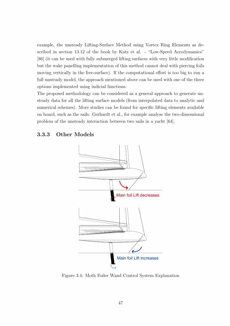
example, the unsteady Lifting-Surface Method using Vortex Ring Elements as de-

scribed in section 13.12 of the book by Katz et al. - “Low-Speed Aerodynamics”

[86] (it can be used with fully submerged lifting surfaces with very little modification

but the wake panelling implementation of this method cannot deal with piercing foils

moving vertically in the free-surface). If the computational effort is too big to run a

full unsteady model, the approach mentioned above can be used with one of the three

options implemented using indicial functions.

The proposed methodology can be considered as a general approach to generate un-

steady data for all the lifting surface models (from interpolated data to analytic and

numerical schemes). More studies can be found for specific lifting elements available

on board, such as the sails. Gerhardt et al., for example analyse the two-dimensional

problem of the unsteady interaction between two sails in a yacht [64].

3.3.3 Other Models

Figure 3.4: Moth Foiler Wand Control System Explanation

47

Some special models have to be implemented to attend to specific needs of special

boats or sailing modes. One of these cases would be when using lifting surface ana-

lytical models with a piercing foil. These simple models do not take into account the

drag generated by the effect of the foil piercing the free surface (generating waves and

spray) or by the horizontal part of the foil working close to the free surface (generat-

ing wave drag). These specific problems are included when using complex numerical

tools such as RANSE codes combined with interpolation schemes. For simpler mod-

els, some analytical corrections can be used. In their Moth VPP [18], in Appendix

C.3.4.3, Bogle et al. present some corrections based on appendage geometry or ap-

pendage coefficient correction based on existing data. More corrections on lifting

surfaces can also be used, such as an effective angle of attack calculation based on

the effect of the presence of a flap or a simple end-plating correction for piercing and

non-piercing lifting surfaces.

Specific models regarding other elements have to be taken into account. For

instance, the possibility of calculating a movable crew affecting the position of the

centre of gravity of the boat and the righting moment should be implemented.

If the boat has some kind of foil control system or flap control system (such as

the wand in the Moth foiler (Figure 3.4)), it has to be modelled. In Appendix A of

[18], Bogle et al. present their analytical model based on forces and moments applied

to the wand and the system geometric characteristics.

3.4 Time-Domain Solver Numerical Schemes

As previously discussed with the forces models, the other major element that has an

important influence on the Simulator behaviour is the way the time-domain Second

Order Non-linear Differential Equations system 3.2 is solved. PASim implements the

following numerical schemes (from simple to more complex):

• Euler scheme.

• Backward Euler (Fixed Point) scheme.

• Backward Euler (Newton) scheme.

• Midpoint scheme.

• Runge-Kutta 4th order scheme.

• Implicit Runge-Kutta 4th order scheme.

48

The details about each method and an explanation of how to implement the nu-

merical schemes is found in “Numerical Recipes. The Art of Scientific Computing”

[143], or other similar books about numerical computation.

The level of complexity (as ordered above) is directly related to the numerical

order of the scheme and the level of accuracy and stability (Higher complexity equals

higher order and higher level of accuracy and stability). The same order is similarly

associated with code implementation complexity and computational requirements,

higher order means higher implementation complexity and higher computational re-

quirements.

The same problems explained for the forces and moments models are repeated

here. The numerical scheme has to be chosen carefully, looking for the one that offers

the best accuracy and stability versus its computational requirements, but always

choosing a method that can be solved quicker than the actual time-domain iteration

time step if the simulator needs to run in real-time.

A specific study has been carried out to illustrate such a dilemma. Even if the

boat chosen as the example for the thesis is the Moth Foiler, the models used are the

ones of a generic America’s Cup 72 boat presented in chapter 8 of Ruiz de Elvira’s

PhD [156]. The reason for this was that when the study was carried out, the models

of the AC72 were more robust and were already tested.

The study consisted of calculating, under specific conditions of True Wind Speed

(TWS) and True Wind Angle (TWA) and reasonable initial values for the adjustment

variables (but without using a pre-calculated VPP equilibrium solution for such val-

ues), a time-domain simulation using the different numerical schemes. The goal was

to verify how the system evolved and whether it was able to reach an equilibrium

state. The initial conditions were a TWS of 7 knots and TWA of 130 degrees. The

initial boat speed was 11 knots and the boat was set sailing in displacement mode

(not in foiling mode), behaving like a conventional catamaran.

For the first time-domain simulations, a large time step (0.5 seconds) was arbi-

trarily chosen to test the potential instabilities of the different numerical schemes in

unfavourable conditions. The total amount of time simulated was set to 50 seconds.

Then the calculated variables were plotted for the different numerical methods. Fig-

ure 3.5 shows the time history of boat speed in knots versus the time in seconds. The

plots of the rest of the variables (heel angle, pitch angle, yaw angle, sinkage, AWS

and AWA) are included in Appendix A.

49

Figure 3.5: AC72 boat speed time history for the different numerical schemes

Because the initial values used for the AC72 time-domain calculations did not

define a situation in which there was an equilibrium of forces and moments, in some

of the calculated variables an initial physical oscillation was induced. In Figure 3.5

for BSP, low order schemes tend to start to oscillate (due to numerical error) to the

point where the models fail to calculate after 39 seconds of simulated time. When

higher order methods are used (Midpoint method and subsequent) the calculations

didn’t present oscillations in BSP and models were able to calculate all the simulated

time. As shown in Appendix A, for the rest of variables, oscillations are present for all

the methods, but for higher order the amplitude tends to decrease while for low order

methods the oscillations amplitude increases especially for the sinkage. It is important

to point out how the different DOF are coupled in the AC72. For example, when the

boat is submitted to a variation in the pitch angle, the amount of vertical force

generated by the foils is changed due to a change in the local AOA. This change in

the vertical force modifies the sinkage of the boat affecting the lateral area, modifying

the lateral forces and consequently changing the yaw and heel angles. If sinkage and

pitch are plotted together, when using high order methods, the oscillations in both

variables are out of phase, helping the boat’s heave stability. If low order methods

are used, due to the numerical induced oscillations, both variables start to enter in

phase amplifying sinkage oscillations as it can be observed in Figure 3.6.

50

Figure 3.6: AC72 pitch and sinkage time history comparison using Euler andMidpoint methods

To verify if the aforementioned BSP oscillations and the amplitude increase for

oscillations in the other variables, that appear when using low order schemes, are

related to a numerical error, different time steps were tested for two different methods,

the low order Euler method and the higher order midpoint method. As it can be

observed in Figure 3.7 (the plots of the rest of the variables are included in Appendix

A), when the time step for the Euler scheme is reduced to 0.1 seconds, the forces

and moments models are able to calculate all the time history up to 50 seconds

but the oscillations in BSP and the amplitude increase for oscillations in the other

variables is still present. If the time step is reduced 50 times (from 0.5 seconds to

0.01 seconds) when using the Euler method, the oscillations in BSP disappear and

the time history matches the one obtained using higher order numerical schemes.

Proving that aforementioned oscillations are related to a wrong selection of the time

step value for low order methods and purely numerical. The midpoint method was

tested with a larger time step of 2 seconds matching the time history obtained with

the same method and a time step of 0.5 seconds (Figure 3.7). This shows that higher

order schemes could be used with larger time steps without losing accuracy for this

particular case.

51

Figure 3.7: AC72 boat speed time history comparison using Euler and Midpointmethods with different time steps

The more reasonable selection for a numerical scheme seems to be the higher order

method that implies the lowest computational effort. For the AC72, the midpoint

method gives the same results as higher order methods such as 4th order Runge-

Kutta. Such a method will be used as the baseline for different boats and situations.

Regarding the selection of the time step to use it is important to point out its

dependency on the inertial properties of the boat, the computational time required by

the calculation of all the forces and moments, the rate of motion cue generation needed

for a proper acceleration reproduction with the Hexapod, the acquisition frequency

of the interface that allows the user to control the simulator and the Virtual Reality

(VR) engine calling rate for updating the boat state vector to the VPP .

A reasonable initial time step that normally satisfies all the exigencies and was

tested with the example boat (Moth Foiler) chosen for the simulator is 0.1 seconds.

Different computational time measurements when executing the Moth models are

presented in Appendix C. They show that 3.3301326 seconds are needed for 1000

executions of a complete set of Moth force models (in this case, a selection of the

simpler models described in Appendix D and characterising all the elements and

parts of the boat) using a single thread execution scheme (please refer to task 7 in

3.6). Therefore, for executing one time the complete set of force models only 0.0033

52

seconds are needed, showing that the execution time is below the time step chosen for

the Moth and ensuring real-time execution. In fact, it gives extra time for executing

the rest of the modules (motion cue generation, Virtual Reality (VR) engine, etc).

Even if there is margin to decrease the time step (from 0.1 to 0.0033 seconds), when

using higher order numerical scheme there is a point where the model did not offer

better results (showed in Appendix A.2 figures). A sufficiently large time step that

allows obtaining a proper solution with the selected numerical scheme is preferable

in order to provide enough margin to fulfil the rest of the simulator computational

needs when solving in real-time, minimizing the number of time steps that have to

be calculated.

It is important to notice that for the selected VR engine (Unigine), described in

Chapter 5, the refresh time for the boat state vector to be reproduced is fixed to

a certain number of frames (images displayed by the engine) processed. The time

step used has to be lower than the refresh time for a specific graphic-card/engine

combination to minimize the error between what it is shown and what it is displayed,

which is the case for the time step selected for the Moth. However, the VR engine can

handle the odd skipped calculations that may happen sometimes in a non-real-time

operating system, such as Windows, in an imperceptible way for the user.

3.5 Autopilots

One of the components that allows the time-domain VPP, and hence the simulator,

to work without multiple human external operation (sailors using the simulator) is

the autopilot. The idea behind the autopilot for a simulator is based on two different

objectives:

• To handle the adjustments of the boat elements in a simulation without the need

for user inputs. For example, in early design stage when analysing the dynamic

behaviour of the boat under certain circumstances, the design team has to be

able to mimic the handling and trimming of the boat using predefined data

and specific algorithms to generate data fast and not depending on the design

team sailing skills and judgement. When the simulator is used for training, the

autopilots allow the simulator to be operated by a reduced sailing crew. For

example, if the training is focused on improving steering of the helmsman, the

other sailors in the boat can be replaced by autopilots. They have a large impact

on the simulator usability and help to reduce the economic cost, becoming an

essential part of the simulator.

53

• To use intelligent autopilots combined with optimization algorithms to deter-

mine the optimum sequence of actions to obtain the best performance in specific

regatta situations such as manoeuvres.

Autopilots are normally related to guidance, Fossen in Chapter 1 of [58] define guid-

ance “the action of determining the course, attitude and speed of the vehicle, relative

to some reference frame (usually the earth), to be followed by the vehicle”. He also

defines control as “the development and application to a vehicle of appropriate forces

and moments for operating point control, tracking and stabilization”. In Ruiz de Elvi-

ras thesis [156], the autopilots definition is expanded as the “criteria established to

the adjustment parameters and/or constraints” to achieve a defined objective. Even

if the autopilot concept is mainly used for the control system in charge of guidance,

in a sailing boat, the course, attitude and speed of the boat depend on the com-

bination of the different tasks carried out by the different crew members (steering,

sail trimming, foils operation) onboard. This is the reason why a new definition of

the autopilot concept will be used all along the thesis associated with the way the

different systems are handled on board the real boat. When a system is meant to

be handled by humans in the real boat, following the more general idea presented by

Ruiz de Elvira in [156], the algorithm in charge of that system will be referred as an

autopilot. If the system is controlled on board by other means than human sailors, the

algorithm in charge of that system within the simulator will be referred as a control

system. However, this definition is not clear for elements controlled by humans with

a pseudo control-system assistance (mainly due to design rule restrictions regarding

control systems on board). For the sake of practicality, these hybrid elements will be

considered as control systems.

The autopilots or control systems will use different information, in order to achieve

the predefined objective. For instance:

• The values of the boat variables to study such as position, velocities, etc (re-

ferred in [156] as space state variables).

• The values of the adjustment variables regarding all the adjustments that can

be made on board to modify the boat behaviour and response (referred in [156]

as adjustment state variables).

• The environmental conditions.

• Different performance and action sequences criteria related to the design goals

and boat reality.

54

This information will be processed by a certain algorithm in order to generate the op-

timum response towards the autopilot objective initially defined. For a more detailed

description of the autopilot scheme implementation suitable for the time-domain VPP

please refer to section 6.3.3 of [156].

One important aspect that has to be implemented inside the autopilots is the one

related to how the adjustments can be made on board. For instance, the autopilot

algorithm can change different adjustments when facing a specific situation but each

one of them needs a certain time of operation until the adjustment is effective on

board (trimming time, energy available on board, etc.). If the time of operation is

not respected then the autopilot will be unable to reproduce the real boat behaviour.

To model the time of operation of a certain element on board, Manuel Ruiz de Elvira

introduced the rate of change of the adjustment in section 6.3.3 of [156], which is used

to limit the amount of change of a certain parameter by time step.

The autopilots have to be adapted for each one of the elements suitable to be

controlled on board. Each one of them will have a specific objective, adjustment

parameters, rates of change and constraints. In fact, the autopilot will be different

not only for each element but it has to be adapted for each situation it will be

involved. For example, when analysing the exit of a tack, the objective (in this

case maximizing boat VMG acceleration) will be different than when maximizing the

VMG in a predefined course. This will also apply to the adjustment parameters, the

constraints and the rates of change of these adjustments.

3.5.1 Boat Elements

For a foiling sailboat the following elements present on board can be suitable to be

used with an autopilot or control system:

• Steering devices:

The principal steering device used onboard is the rudder and its associated

adjustment variable is the rudder angle. When the autopilot is used to control

this type of device, the objective will depend on the task to fulfil. When used

in the dynamic analysis of certain manoeuvres, the objective can be as simple

as maintain the boat heading, maximize VMG under certain environmental

conditions, minimize the distance between two geographical waypoints, etc. For

a simulation of a complete regatta, the autopilot has to be connected with an

RMP module in combination with the autopilot objective (normally maximize

VMG) to have enough strategic information to generate a realistic handling

55

behaviour. This simulator autopilot is what is usually known as an autopilot in

other industries.

• Sails:

Normally the objective is to generate the amount of driving force and heeling

moment with the available righting moment to generate the fastest boat speed

or the maximum acceleration. Other objectives for manoeuvres such as a tack

can be minimizing the loss of distance to windward during the tack. The au-

topilot can use a simple de-powering scheme (like the one presented in [33]) as

adjustment variables or if the aerodynamic sail model implemented is based on

multiple trimming parameters as part of the model parametric space it can use

such trimming parameters as adjustment variables.

• Foils:

Related to aircraft flight controls, the foils objective normally aims to maintain

a certain ride height or a specific boat attitude to minimize dynamic instability

and drag. The adjustment variables depend on the adjustment capabilities of

the foils, the most complex systems nowadays allow to rotate the foils in three

axes (cant, rake and toe) and one translation (foil up and down). The foils

can be controlled by sailors or a control system, in fact, if the control system

is based on mechanical devices using force inputs, such control systems can be

modelled as special forces and moments models as explained in 3.3.3.

• Energy generation and management system:

The energy on board is normally limited and generated by human power (whose

generation capacity decreases quickly with time and sustained load, a factor

that has to be taken into account in the system model). The objective of

the energy control system is to generate, manage and deliver the maximum

amount needed in such a way that all the consumers on board (all the electric,

hydraulic or pneumatic powered elements) receive what they need at any time,

to fulfil specific operations, without consuming the total amount available, and

knowing the energy generation capabilities (using the time operation concept

introduced previously). If different operations have to be done at the same

time and the energy available does not fulfil all the instantaneous requirements,

the control system has to be prepared to deliver the energy to the element as

soon as is available or to prioritize the delivery to a specific consumer based

56

on its importance in the manoeuvre being made. The adjustment variables

are normally related to the number of grinders available and how the energy is

distributed to the different onboard systems.

• Crew position and moveable masses on board:

The position of the centre of gravity of the boat affects the amount of righting

moment available and the boat’s attitude. The objective with such elements is

to maximize the righting moment available (to be able to generate more driving

force with the sails) or to keep a certain boat attitude (for example to control

pitch dynamics in the Moth foiler changing, the foils angle of attack leading

to dynamic instabilities). The adjustment variables are the centre of gravity

position over the deck for the crew or the quantity and the centre of gravity

position inside the boat for a movable mass.

Each autopilot represents an added layer of complexity inside the VPP. In fact,

each crew member (or following the simulator analogy each autopilot) communicates

to each other in order to execute the task that he is assigned to. The main difficulty

with autopilots is to allow the communication and interaction between each autopilot

in order to obtain the best performance. This can be relatively easy when the objective

for all the working autopilots for a specific simulation is the same. Otherwise, this

can be addressed using a general autopilot with a weighted objective function taking

into account all the objectives for each individual autopilot.

3.5.2 Algorithms

All the autopilots and control system algorithms are based on control theory, but

an in-depth analysis of such topic is out of the scope of the thesis. An extensive

research has been already done regarding marine vehicles control and guidance, such

as the work made by Tristan Perez in ship motion control (course keeping and roll

stabilization) in [131], or the work carried out by Fossen in his book “Handbook of

Marine Craft Hydrodynamics and Motion Control” [59]. Other research has been

done on specific marine vehicles, such as autonomous underwater robots like the one

carried out by Somolinos in his thesis [162], or autonomous sailing boats like the

one made by Cruz et al. in [34]. Different control algorithm options can be used and

applied for the different autopilots and control systems, at least with the conventional

displacement sailing boats, and some of them will be highlighted in the following list:

• Pre-introduced data:

57

It is the simplest way to implement an autopilot but it is not considered as

a control algorithm. It is based on a predefined time-domain set of actions,

regarding the adjustment variables, to be performed along the simulation.

• Proportional-Integral-Derivative (PID) control algorithms:

The PID controller is a control loop feedback mechanism that can be applied

to the different elements present onboard (mainly steering devices). Fossen in

Chapter 12 of [59] explores the use in marine applications. Ruiz de Elvira in

[156] explores their implementation in the time-domain VPP autopilots.

• Advanced Control algorithms:

As introduced by Fossen in Chapter 13 of [59], optimal and non-linear control

algorithms and techniques can be used in marine applications. Among those ad-

vanced control algorithms, we can find linear quadratic optimal control, sliding

mode control, state feedback linearization and integrator backstepping.

• Neural networks algorithms:

As part of intelligent control, the neural networks can be used to generate au-

topilots for the different systems onboard. To be able to use them, the neuronal

networks that will handle the different elements have to be trained using a set

of input-output data. This data describes the behaviour of the element to be

controlled under the influence of a certain input. Priandana et al. in [144]

present the usage of such type of control for a double propeller boat model.

It is important to note that foiling sailboats are dynamically closer to aeroplanes

than to the conventional displacement sailing boats. This is the reason why autopi-

lots and control systems for conventional boats have to be adapted for the dynamic

problems of foiling boats, or other solutions have to be implemented. Foiling sail-

boats present a wider range of dynamic stability problems that have been already

studied in aircraft. For example, the pitch stability in a foiling boat resembles an

aircraft, the control system implemented for the aircraft to avoid this specific issue

can be used for the same purpose in a foiling boat. Extensive research has been made

regarding aircraft stability and control systems and is presented in a large number of

publications: [49],[29], [163], [110].

58

3.5.3 A General Approach for Neural-Network-Based Au-topilots

The neural network can potentially be used for the different elements autopilots within

the simulator. A similar implementation to the one proposed by Lewis et al. in [98]

for robots can be adapted to mimic a specific sailor behaviour performing a specific

task on board. A generalized approach based on a multilayer neural network con-

troller combined with simulator generated input-output data obtained by repeatedly

simulating manoeuvres and regattas in different situations during crew training is

potentially the most general approach that can be implemented inside the simulator.

Using the sailors that will sail the real boat to generate input-output data during the

simulator training time allows obtaining good quality neural network training data

(avoiding on the water measurement problems) that can potentially mimic implicitly

the strategies and reflexes of the crew within the generated autopilots following the

idea of modelling human performance using neural networks presented by Fix et al.

in [54]. The generalized approach presented before uses an off-line learning procedure

for an open-loop autopilot. An advanced version can be implemented when combin-

ing off-line preliminary learning with sailor simulator training generated input-output

data and an on-line learning procedure combining neural networks with adaptive con-

trol theory in a closed loop scheme, introduced in section 1.3 of Lewis et al. [98] and

developed later in the same work for robot applications, when the autopilots are being

used.

3.5.4 The Simulator as a Safe Test Environment for ControlSystems

Control systems are an important part in some of the new foiling sailboats, in fact,

they are used to control onboard foils and other elements and systems. Real scale

testing of such control systems is expensive and potentially dangerous for the material

and the crew sailing the boat. The simulator not only uses the autopilots and control

system models but it can also be inexpensive and a safe environment to test the

behaviour of the different control systems present on board. In fact, it can be used

in combination with other tools such as the genetic algorithms to optimize and fine-

tune the control system parameters to improve its robustness and the overall boat

performance.

59

3.5.5 Use of Autopilots to Improve Performance

Autopilots allow making a wider use of the simulator even if the different tasks on

board are not performed inside the simulator by a human user. In some situations,

their use can also help to improve boat performance. Specific manoeuvres or regatta

situations can be reproduced multiple times using intelligent neural-network based

autopilots with an on-line learning scheme, like the one explained in 3.5.3 and time

history data is generated. Then, the same data is collected when the sailors reproduce

the same manoeuvres, training in the real boat or in the simulator. If the collected

data shows different performance in comparison with data generated using autopilots,

the time history of the different elements can be analysed to determine corrections to

the way sailors are performing their specific tasks on board simpler.

Following the same idea, the sequence of actions (the order of the different actions

made on board to face a manoeuvre or a regatta situation) towards a better perfor-

mance can be determined using autopilots combined with Genetic Algorithms(GA).

In fact, the sequence of actions can be modelled associating a different integer value

for each action and generate with those integers a vector that will be the input pa-

rameter of the GA algorithms. The GA algorithms will iterate changing the order of

the elements present in the vector (and therefore changing the sequence of actions)

towards fulfilling the problem objective of maximizing performance. The performance

objective will be expressed via a merit function that has to be determined to fit each

manoeuvre or regatta situation.

3.5.6 Unstable Boats

As it will be explained later, the boat chosen for the thesis is the Moth foiler, a small

dinghy equipped with foils and unstable behaviour. For the time-domain simulations

presented in [18], a PID controller is used to maintain boat course. To avoid roll

instabilities, in [18] the roll is fixed in order to allow a proper control of the PID

in charge of the rudder. Following a similar approach, a specific heel angle control

scheme using a PID controller is developed. In order to simplify the problem, the

heading is locked during the PID tuning and testing stages. The numerical scheme

used for the tests is a fourth order Runge-Kutta with a time step of 0.1 seconds,

in order to avoid inducing large numerical errors in the simulation. The heel angle

control scheme is based in two elements, a roll moment variation procedure using the

elements available on board (the sail trim via the flat variable from the depowering

60

model implemented, as described in Appendix D, ranging from 0.1 to 1, and the

crew position via the Y position variable of the crew centre of gravity referred to

the sail boat centreline, ranging from 0 to 1.250 meters) and the PID. The PID

controller calculates a control variable, ranging from -1 (overpowered situation) to 1

(underpowered situations), based on the heel error and managing the roll moment

variation procedure. This procedure consists of:

• When the boat is underpowered (PID generated variable < 0):

– If the sail trim parameter can be increased (not at its maximum value),

increase its value until the PID variable requirement is fulfilled.

– If the sail trim parameter reaches its maximum value move the crew in-

board until the PID variable requirement is fulfilled or the Y crew minimum

position is reached.

• When the boat is overpowered (PID generated variable > 0):

– If the sail trim parameter can be decreased (not at its minimum value),

decrease its value until the PID variable requirement is fulfilled.

– If the sail trim parameter reaches its minimum value, move the crew out-

board to increase righting moment until the PID variable requirement is

fulfilled or the Y crew maximum position is reached.

Because the effects on roll moment of the sail trim parameter and the crew position

are different (the flat variable affects more the roll moment than the crew position per

unit change), the change rate on both variables is normalised in order to generate the

same response per unit change in the transitional area every time the PID variable

changes.

After implementing the heel control procedure, a PID tuning has been held. The

main problem found when trying to obtain the different PID coefficients was related

to the Moth inherent roll instability. In fact, the boat was not able to reach a sta-

ble state after a step change in the heel PID setpoint (target heel) or in the wind

conditions (TWS), leading to a boat capsize. The traditional tuning methods were

difficult to apply because of the large oscillations obtained and subsequent simulated

boat capsize. Using a minimal step change (0.1 degrees of heel in the setpoint) with

the Ziegler-Nichols tuning scheme combined the Pessen Integral Rule (as introduced

by Pessen in [134]) allowed to determine the critical gain (Ku = 0.25) and roughly

estimate the corresponding period of sustained oscillation (Tu = 7s). This tuning

61

procedure presented the best results among the traditional techniques when obtaining

an initial PID coefficients estimation, that was later refined by manual fine-tuning

to improve the PID behaviour. In order to obtain better results, a Genetic algo-

rithm training scheme for the controller coefficients has been implemented using the

Differential Evolution algorithm (a mono objective optimization algorithm presented

by Storn et al. in [166]) applied to a PID setpoint (target) step change situation.

The objective function, in this case, was the sum of the absolute value of the PID

error each time step. In order to account for early capsizes, these situations were

penalized using a high error value for each time step after the capsize, even if the

total time-domain simulation time was not reached. Both techniques lead to similar

coefficient results (the order of magnitude of the coefficients obtained is: 10−4 for Kp,

10−4 for Ki, 10−1 for Kd) and the heel PID controller allowed the simulated boat to

maintain its behaviour for more than 30 seconds when it was not subject to changes

in the external conditions. The PID controller managed to maintain the boat’s heel

during the first 18 seconds by changing flat and crew position variables in steps lower

than 10−3 as it can be observed in table B.1. The last simulated seconds, the PID

tried to correct larger changes in heel leading to an uncontrolled oscillation of the

total moment around the X-axis, as it can be observed with more detail in table B.2.

With larger values of the coefficients, the simulated boat crashed after a few seconds

of simulation. When the PID controller with the determined coefficients was used

in simulations where external conditions changed (a larger variable change rate is

needed), it was not able to control the heel and avoid capsize. This suggests that

in highly unstable boat situations, like the roll unstable behaviour of the Moth due

to its lack of roll inertia, a simple PID controller is not a suitable option. In these

situations, an adaptive method has to be used in order to adapt to the changing con-

ditions, such as a PID combined with fuzzy logic or more advanced control systems

based on stochastic control theory such as a Linear-Quadratic-Gaussian controller (a

combination of a Kalman filter, a linear-quadratic estimator and a linear-quadratic

regulator). In Table B.1 of Appendix B, the time history of the simulated Moth

run using the heel PID controller described above and the force models (described in

Appendix D) are shown with a time interval of one second.

62

3.6 A Note on Multi-Threading Execution and Multi-

Computer Configuration

The main goal for a practical simulator is to be able to calculate forces and moments

models and to solve numerically the second order non-linear differential equations

(3.2) in less time than the actual time step. When a high level of accuracy is needed

(for instance being able to solve numerical schemes), a multi-threading approach has

to be used. Being able to run all the models in multi-thread configuration creates the

capacity to substantially reduce the execution time of an individual iteration. The

main problem is related to the way the VPP is structured. For instance, in each time

step, every forces model has to be calculated before the time-domain equation system

will be solved. With an optimum configuration of one thread per model, the minimum

execution time to calculate the models will be the time needed to calculate the slowest

one. Some models depend on other models, like when a foil with a flap model has to

be calculated after the model of the control system that manages the flap behaviour,

reducing the value of using multi-threading. The reduction in computational time

will be useful but limited (never divided by the number of threads available).

Nine tests were carried out to measure the time-saving improvement using multi-

threading when calculating with the Moth foiler models. The forces and moments

models (described in Appendix D) were divided into blocks, containing each of the

boat elements to be calculated, for instance:

• Block 1: Calculating the models related to the wand control system.

• Block 2: Calculating the models related to the rudder and its horizontal foil.

• Block 3: Calculating the models related to the hull.

• Block 4: Calculating the models related to Board and its horizontal foil.

• Block 5: Calculating the models related to the sail.

• Block 6: Calculating the models related to the windage.

• Block 7: Calculating the models related to the gravity forces.

• Block 8: Calculating the models related to hydrostatics.

Because of some model dependence (mainly between the wand control system and

the board) different execution procedures were used:

63

• Running the models in blocks.

• Running the models in tasks (based on model dependence):

– Task 1: Execution of block 1 and 4.

– Task 2: Execution of block 2.

– Task 3: Execution of the rest of the blocks.

The final tests configurations used are:

• Test 1: Running 1000 times each block using one independent loop per block.

Using a thread for each block loop iteration in a thread pool architecture with a

4 threads processor with all the threads available. Waiting for each block loop

to be finished to start the following one.

• Test 1*: Running 1000 times each block using one independent loop per block.

Using a thread for each block loop iteration in a thread pool architecture with

a 4 threads processor with all the threads available. Executing all the loops at

the same time.

• Test 2: Running 1000 times each block using one independent loop per block.

Using a thread for each block loop iteration and waiting for each block loop

iteration to be finished to start the following one.

• Test 3: Running 1000 times each task using one loop per task with a 4 threads

processor with three threads available, one thread for each task. Waiting for

each task loop to be finished to start the following one.

• Test 3*: Running 1000 times each task using one loop per task with a 4 threads

processor with three threads available, one thread for each task. Executing all

the task loops at the same time.

• Test 4: Running 1000 times each task using one general loop for all the task

with a 4 threads processor with three threads available, one thread for each

task.

• Test 5: Running 1000 times each block using one independent loop per block

without using multi-threading.

• Test 6: Running 1000 times each task using one loop per task without using

multi-threading.

64

• Test 7: Running 1000 times each block using one general loop for all the blocks

without using multi-threading.

All the time measurements are presented in Appendix C. The most realistic situ-

ation taking into account other processor loads and model dependence is the configu-

ration used in test 3* presenting a time saving of approximatively 45% in comparison

with the same configuration without using multi-threading which correspond config-

uration 6.

When looking at the general picture, the simulator uses more elements than the

actual time-domain VPP. It needs computational resources for the generation of mo-

tion cues for the Hexapod, the Engine managing virtual reality and visualisation and

the acquisition system behind the user physical interface. In a scenario where even

the execution of the core of the simulator (PASim) could present a lack of resources,

a new approach has to be designed. Having the ability to use multiple dedicated

computers to run each of the components individually seems the best solution. In or-

der to ensure proper and fast communication the network protocol UDP described in

[141] is implemented in each simulator component and modern network architecture

has to be used (Gigabit Ethernet) in each computer and network hardware.

3.7 An Example : The Moth Foiler

When the idea behind the simulator was first started the boat candidate for testing the

concept was chosen. Instead of choosing a more conventional boat, the approach was

to select an apparently simple and little foiling boat but very complex dynamically

and very unstable to really pushing the boundaries of the technology in existence.

The chosen candidate was the Moth Foiler.

65

Figure 3.8: Moth sailing in foiling mode.Photograph by Manuel Ruiz de Elvira

3.7.1 The Boat

The International Moth Class is a boat class that manage the Moth foiler fleets. As

specified in their website [4], the Moth is a sailing dinghy with the following general

characteristics:

• Length overall: 3.355 m.

• Beam: 2.250 m.

• Max. luff length: 5.185 m.

• Max. mast length: 6.250 m.

• Hull weight: Unrestricted, general weight range 10-20kgs.

• Rigged Weight: as little as 26kgs.

66

• Sail area: 8.25 m2.

• Restrictions: Multihulls, trapezes, moveable seats and sailboards are prohibited.

• Optimum skipper weight: 60-80kgs.

As explained in the class rule[3] number 1, “The International Moth is a single-

handed development class boat” with “open class rules”. It is the result of many

years of development since its initial conceptualization in 1928, that has included,

across this history, the use of lightweight hulls and big sail area. Presently, it is one of

the fastest single-handed monohull dinghies in production, capable of reaching more

than 30 knots sailing supported on its foils. The class has contributed to the foiling

boat’s development since the 1990s as explained in [177] and now is one of the most

active foiling boat classes in the world

The boat configuration consists of:

• A narrow carbon fibre hull with hiking wings.

• A carbon fibre mast.

• Only one mainsail.

• A daggerboard T foil with a flap controlled by a Wand system.

• A rudder T foil.

The boat could be observed sailing in foiling mode in figure 3.8.

3.7.2 Forces and Moments Models

The following forces and moments models try to represent the physics involved while

sailing the Moth. All the details regarding those models are explained in Appendix

D. The models are sorted by the type of element:

• Aerodynamic Models

– Sails

∗ Bogle et al. [18] Aerodynamic Model based on North Sails Flow data

combined with Heikki Hansen work [72] sails coefficient curves mod-

ified to include the last IMS flat and associated twist function de-

powering scheme. (Mixed model)

67

∗ Aerodynamic model based on the TFWT (University of Auckland)

data collected by the author. (Interpolated Model)

∗ IMS model. (Analytical model)

– Windage

∗ General model based on Bogle et al. [18] work with improvements

and corrections (For rig, crew, hull and emerged appendages below

the hull). (Analytical model)

• Hydrodynamic Models

– Lifting Surfaces (Daggerboard and Rudder T-foils)

∗ Elliptical distribution lifting line. (Analytical model)

∗ Complex Lifting Line. (Numerical model calculated in execution time)

∗ VLM. (Numerical model calculated in execution time)

∗ End-plating and Piercing corrections. (Analytical model)

– Hull

∗ Hull model based on raw data from Beaver et al. paper [10] (with hull

hydrostatics incorporated). (Interpolated Model)

• Other Models

– Control Models

∗ Improved and completed version of Bogle et al. [18] Wand control

model, using a Newton numerical scheme for finding equilibrium of the

Wand system forces and moments. Normal or paddled wand version

with different level of complexity available. (Analytical model)

– Other hydrostatics and weight stability models

∗ Yacht and crew weight model (with crew optimization). (Analytical

model)

∗ Appendage hydrostatic forces model based on immersed volumes and

centres calculation. (Analytical model)

The following selection of the models presented above was used to generate the

polar curve for the boat of Figure 3.9 and during Moth time-domain simulations such

as the ones presented in Appendix B:

68

• Bogle et al. [18] Aerodynamic Model modified to include the last IMS flat and

associated twist function de-powering scheme.

• Improved and corrected Windage model based on Bogle et al. [18] work.

• Complex Lifting Line with End-plating and Piercing corrections for all the lifting

surfaces.

• Hull forces model based on raw data from Beaver et al. paper [10].

• Improved and completed version of Bogle et al. [18] wand control model.

• Yacht and crew weight model (with crew optimization).

• Appendage hydrostatic forces model based on immersed volumes and centres

calculation.

69

Figure 3.9: Moth polar curve generated using PASim.

3.7.3 An Example of the Foiling Moth Simulator Usage: TheTransition Study From Non-Foiling to Foiling

The simulator can be used to study specific dynamic situations that will affect foiling

boat performance on the water. For example, the simulator was used to study the

acceleration capability of the foiling Moth while transitioning from a non-foiling to a

foiling situation caused by an increase in the wind speed.

The time-step used in this simulation was 0.1 seconds combined with the midpoint

numerical scheme. The initial values were obtained from a pre-calculated equilibrium

70

condition of the boat sailing in 6.7 knots of TWS, a TWA of 90 degrees and 4.892

knots of BSP with the yacht sailing in displacement mode. A gust was generated

changing the TWS from 6.7 knots 10 knots during the first 6 seconds of the simulation,

maintaining the higher wind speed after that. In order to maintain the heading and

the heel angle, a set of settings (rudder angle, crew position and flat sail trim setting)

were adjusted in every time-step to maintain the total moments around the X-axis

(Mxx) and Z-axis (Mzz) equal to zero. In order to help the transition, the crew X

position was moved from the initial equilibrium position near the centre of the hiking

wings to the rear of those wings, correcting the boat pitch angle. The crew Y position

and flat sail trim variable were used to correct Mxx. The rudder angle was used to

correct Mzz. The total simulated time was 35 seconds.

As it can be observed in Figure 3.10 the boat was able to accelerate from 4.892

knots to 12.686 knots of BSP after 35 seconds, foiling after 16 seconds at 8.949

knots of BSP. The wand system was able to maintain the boat height close to 0.55

meters above the water after taking off (Figure 3.11). Repeating this simulation with

different parameters of the wand control system can be used to evaluate its effect on

the transition. The boat pitch angle increased during the transition to reach a new

position after the transition.

This is just a simplified example to show how this type of study can be used to

optimize crew movements and onboard adjustments to refine the athletes technique

using all the simulator resources available (visual cues, kinematic cues, etc) for an

easier and more efficient training. However, it is important to note that despite the

simplicity of this simulation, it involves some not-obvious considerations such as the

fact that the movement of the crew causes a change in the yachts inertias (with the

crew representing 2/3 of the total weight) and the generation of a force on the yacht

by the crew to make that movement happen.

The data of the complete simulation (in time-steps of 1 second) can be found in

Table B.3 Appendix B.

71

Figure 3.10: BSP time history of the Moth foiling transition.

Figure 3.11: Sink time history of the Moth foiling transition.

72

Chapter 4

The Motion Platform

As explained in chapter 1, the simulator is a combination of different components in

charge of reproducing specific aspects of the physics behind sailing. The component

in charge of reproducing the physical sensations related to movement or acceleration

is the motion platform. This platform will be different depending on the degrees of

freedom needed for each type of boat. The simulator as a general tool has to be able

to calculate all the cues needed for every configuration or at least the boat variables

needed for it. For a general overview of the motion platform implementation within

the simulator please refer to the diagram in Figure 2.1. For a specific overview of this

module implementation please refer to the diagram in Figure 4.1. All the elements

within this module will be described in the following sections.

73

Figure 4.1: Motion platform module block diagram

4.1 The Degrees of Freedom

The first aspect that will determine the number of kinematic cues to be reproduced

is the type of boat that will be simulated.

4.1.1 Conventional Monohulls and Slow Multihulls

As explained in chapter 3, even if the time-domain VPP could carry up to 6 DOF

calculations, for slower boats the reality could be reproduced with no more than 3

or 4 degrees of freedom (ORC VPP uses 2.5 degrees of freedom with successful boat

performance prediction [33]). In fact, when trying to simulate such situations, in

the past, only one kinematic cue was reproduced (at least in more or less calm sea

74

conditions, because waves could induce boat movements and accelerations). This

approach was used for the first commercial simulator, the VS-1, presented in [12]. In

this case, a real dinghy hull was mounted into a specific rig able to reproduce the

heel angle motion. If waves are taken into account or a more realistic reproduction

is desired, a rig capable of reproducing heel and pitch motion could be used. A

full 6-DOF approach could be useful for such boats and was used in past monohull

America’s Cup campaigns. In fact, when a fully dynamic situation has to be studied

(for example how the boat will accelerate after some situations) a 6-DOF approach

will be the option to choose. Normally, the number of kinematic cues reproduced

has to be equal or lower than the DOF calculated by the VPP. In fact, even if a

6-DOF approach is used, the number of kinematic cues reproduced are related to the

dynamic characteristics of the boat and the goal of the study carried out with the

simulator (sometimes simpler rigs could be used). However, for fast planing boats

such as the 49er dinghy (observed sailing in figure 4.2) a full 6-DOF/6-DOF approach

could be preferable (using the sailboat 6-DOF for the calculations within the VPP

and a platform capable of reproducing 6-DOF of motion). For slow multihulls (like big

cruising catamarans) the same principles declared for monohulls have to be applied.

Figure 4.2: 49er dinghy sailing.Photograph by local Geelong yachtsman.

Source: https://commons.wikimedia.org/wiki/File:49er_skiff_sailing_AUS_nationals_Geelong.jpg

4.1.2 Fast Multihulls and Foiling Boats

When dealing with fast boats, which sail by generating high AWS with low AWA

(generally fast multihulls and foiling boats), fewer options are available. The sailors

of these kinds of boats are used to sailing the boat according to their own trained

way to feel the boat’s physical behaviour. Proper reproduction of every kinematic

75

source available is needed to be sensed by the simulator user. Different solutions

could be adopted to reproduce the boat motions. Even if the usual solution is to

use a Stewart 6-DOF parallel robot (Hexapod) [164], special configurations could be

developed when a specific degree of freedom is out of the motion and acceleration

range of the platform or it is predominant over the others (motion platforms 6-DOF

expanded approach). For example, in sailboats heel could be considered separately

because of its higher amplitude range. Special prototypes have been developed to

face this kind of problem, like using a combination of a Hexapod moving over a

linear rail (such as the Mercedes-Benz Driving Simulator [113]) or the special cable-

driven parallel robot developed by Fraunhofer IPA and Max Planck Institute for

Biological Cybernetics (MPI) [106], where highly dynamic simulations with complex

acceleration patterns could be reproduced. For these kinds of boats (like the Moth

Foiler, the AC50 or displacement catamarans such as the AC45 version without foils

presented in figure 4.3) the 6-DOF/6-DOF approach (using the sailboat 6-DOF for

the time-domain calculations inside the VPP combined with a platform capable of

reproducing 6-DOF of motion) or 6-DOF/6-DOF expanded configuration approach

should be used.

(a) (b)

Figure 4.3: AC50 (a) and AC45 (b) sailing.Photographs by Manuel Ruiz de Elvira

4.2 Reproduction of Motion and Position Versus

Reproduction of Rotational Velocities and Lin-

ear Accelerations

Other considerations have to be taken into account, to determine which type of kine-

matic motions will be reproduced. Two different philosophies could be used, to re-

produce the full motion (which implies also the reproduction of the acceleration) or

76

to reproduce linear accelerations and rotation velocities. It will depend mainly on

the number of DOF to reproduce with a specific technology and also on how the

visualisation system will be mounted and used.

4.2.1 A Tool to Reproduce Motions and Position

When a low number of kinematic cues have to be reproduced (one or two cues) simpler

rigs could be used. For instance, a frame combined with one or two electric linear

actuators could be enough to reproduce the boat exact angular motion and position

for heel and pitch (in a boat sailing in normal circumstances) without reaching the

rig angular limits. This setup is similar to the ones used in [12] and [116]. When the

calculated boat motion is reproduced, after evaluating the feedback from experienced

sailors, Mulder et al. in [117] concluded that the most engaging motion to contribute

the sense of presence for conventional boats is the roll motion and the pitch motion

(but only when combined with the roll motion). During Mulder’s et al. study, other

motions, such as heave, degraded the sense of presence. This can be related to the fact

that the visualization system is not offering the level of realism needed (the screen is

not large enough or the motion cues do not follow the graphics) or the VPP models

do not generate the proper cues. In fact, when the visualization system is mounted

outside the moving platform (for example using screens fixed to the wall instead to

the platform in charge of reproducing the kinematic cues like in [117]) it is important

to be able to reproduce the motion precisely following the graphics movement. If

the user is able to identify the visualization system as something uncoupled from

the platform, he has more visual references that help him to know exactly if the

motion system is acting in a proper way. If the platform is able to reproduce a large

number of motion cues, the user looking at the screen will be more aware of moving

differently than the fixed screen, degrading the sense of presence. In foiling and fast

boats, sensing boat behaviour is a vital part when handling the boat. In fact, it is

important not only to the helmsman but also to the crew that does not have a visual

reference of the boat moving (for example a trimmer looking to the sail). In this case,

kinematic cues have to be reproduced for the 6-DOF and other techniques have to be

used to avoid that presence degradation.

Motion and position reproduction should be used for some specific tasks when

using the Simulator. One such task, described in section 2.2.6, is testing deck gear

and deck layout configurations. With the one-to-one scale deck mock-up mounted

on top of the 6-DOF platform, the skipper and the engineers could test the gear

layout while moving the platform to specific sailing positions (could be obtained

77

by calculating VPP equilibrium solutions) or reproducing predefined accelerations

patterns (generated by specific time-domain analysis with the VPP) cyclically.

4.2.2 A Tool to Reproduce Rotational Velocities and LinearAccelerations

To overcome the problem previously presented, while trying to reproduce a big num-

ber of motion cues, a different approach has to be used. In fact, it has been present in

the aeronautic simulation industry for years (used in Full-Flight Simulators (FFS) for

pilot training). The approach consists of mounting the visual system inside a closed

space on top of the simulator to isolate the user from the outside. Being isolated

prevents the user from taking spatial references external to the simulator. In vehicles

with closed cockpits the problem is easily solved. For example, for jetliners, a repro-

duction of the nose of the plane mounted on top of the platform with projected images

in the plane’s windows will be enough. For open cockpits configurations, which is the

case with sailing boats, the task becomes more complicated and a wide range of view

has to be covered (in fact, for an ideal experience the whole 360-degree range of view

has to be represented). The full range of view could be covered using Virtual Reality

headset, but such devices have their own associated problems as will be described in

the following chapter.

As explained by Dichgans et al. in [46], self-motion perception is mainly related

to the interaction of the human visual and vestibular systems subjected to visual

stimulations, rotational velocities and linear accelerations. Harris et al. in [75] explain

that linear acceleration can be also be sensed by:

• Specialised visceral graviceptors (that can be found specifically in the region

of the kidney) but with a poor directional estimate. Such receptors will be

stimulated at the same time as the vestibular system while using motion cue

generation. Because the motion platform will stimulate the whole body at the

same time the effects of these receptors are considered included in the vestibular

system.

• The somatosensory system via pressure and stretch detection on the skin and

in muscles, joints and visceral organs (for example when a subject is seated

and undergoing vertical acceleration, the body parts in contact with the seat

will have the cutaneous receptor stimulated because of the forces generated).

Such perceptions are located in specific body parts and could be stimulated in

absence of motion by exerting pressure over certain areas. Such methodology

78

could be useful for seated handling situations (for example in planes) but not

for the usual sailing boat handling positions.

They also explain that self-motion perception could be sensed by the so-called

proprioceptors (some of the systems and receptors described above could be included

inside), but the proprioceptive system is normally in charge of determining relative

movement of body parts. Like the somatosensory system, this system will not be

specifically stimulated.

If we consider the simulator as a global self-motion perception problem (where

the goal is moving the whole user body), then the solution seems to be to generate a

combination of visual and vestibular system stimulations. The visual stimulus should

be reproduced using a realistic visualization system and rotational velocities and linear

acceleration should be reproduced using a physical device in a full 6-DOF or extended

6-DOF configuration (using a Stewart 6-DOF parallel robot or a combination of the

same robot with linear rails or angular movement devices). Instead of developing

a specific approach with specific body parts stimulation (that could be used in a

seated simulator handling situation), the approach proposed for this thesis will be

to stimulate the whole body at the same time, allowing the reproduction of multiple

types of boats using the same simulator configuration with very few changes. This is

the same philosophy adopted in the time-domain VPP.

Within the simulation industry there is discussion regarding whether or not it is

necessary to generate all the stimulations described previously or if a good amount

of realism can be achieved using only the simulator visualization system. Burki-

Cohen et al., in [23], discuss the problems associated with the usage of a Stewart

platform for vestibular cueing and explain the limited reliability of the vestibular

system (loss of sensitivity after repeated stimulation and spatial disorientation after

unusual motion cues). They propose the use of other motion cues than the visual and

vestibular ones (the proprioceptive and tactile stimulations). They also present and

compare other advanced motion simulation technologies such as the NASA Vertical

Motion Simulator (VMS), the centrifuge motion simulator - Wyle’s Dynamic Flight

Simulator (WDF), the Desdemona Simulator combining a 6-DOF platform with a

centrifugal design or even the In-flight Simulator using actual aeroplanes to mimic

other aeroplanes. Such systems try to overcome the limited capability of the Stewart

platform when generating sustained acceleration, following the same concept as the

already mentioned 6-DOF expanded configuration. The selection of a system based

79

on a 6-DOF motion platform implies a high economic cost, a cost-saving alternative

is explored in [23], the dynamic seat which is able of generating some vestibular,

proprioceptive and tactile motion cues in a fixed-based trainer. These solutions are

oriented for aeroplane simulation but motion patterns in boats are different from the

patterns in aeroplanes. The cockpit layout and user position in a sailing boat are not

suitable to solutions like the dynamic seat so more conventional approaches such as

the Stewart platform, where the user has more freedom to move, are preferable.

Other problems (not associated with the concept of presence and realism) are

involved. For example, as explained by Howard in [78], the visual, vestibular and

proprioceptive information received by humans help to solve ambiguities when deal-

ing with an orientation and self-motion situation. McCauley et al. in [109] explain

that such ambiguities could be created by the Virtual Environments when generating

visual, but not vestibular, stimulation. Welch, in [187] and [188], explains that the

human perception system is able to adapt itself and compensate for changing con-

ditions. Such stimulation ambiguities could also trigger motion sickness instead of

adaptation.

Following a general approach, the configuration of an integrated visualization

system combined with a 6-DOF motion platform is the solution chosen for this thesis.

More precisely the physical platform used and implemented in the simulator will be

a modern, electric actuated version (cheaper in maintenance and more reliable than

the hydraulic implementation) of the 6-DOF parallel robot known as the Stewart

platform. To overcome the inherent limitations of such a configuration a washout

filtering system is also implemented and will be explained later. As a modular system,

when using the simulator, motion cues could be deactivated if needed (when a motion

system is not in use because of economic reasons or due to lack of space). Alternative

motion cue generation algorithms could be implemented to fit other motion systems

like the 6-DOF expanded configuration.

4.3 The Stewart Platform: A Six Degrees of Free-

dom Parallel Robot

The motion platform selected as the base case in the thesis is the Stewart platform

manipulator. A brief description of such a manipulator will be developed and the

chosen inverse kinematic and dynamic algorithm will be described qualitatively.

80

4.3.1 Description

The main solution adopted in the state of the art simulators (at least outside the de-

velopment of experimental simulators) is the 6-DOF parallel robot (Hexapod) known

as the Stewart (or Stewart/Gough) manipulator (or platform). As comprehensively

described by Dasgupta et al. in their platform review [41], the Stewart platform ap-

pears for the first time in Stewart’s paper [164], where a 6-DOF device was used to

simulate flight conditions. The device presented in this paper had a different geom-

etry than the one we know today (a triangular upper platform combined with three

adjustable legs combined with two-axis joints). In fact, Gough proposed the use of

a fully parallel approach using a combination of six linear actuators (closer to the

configuration of the tyre testing machine presented by Gough et al. in [67]).

Far from the initial designs and proposals, presently the generalized Stewart platform

or manipulator is composed of two rigid bodies (the platform and the base), six linear

actuators with two joints each, attaching each actuator to the base and the platform.

It could be found in two main joints configurations:

• The 6-SPS (spherical-prismatic-spherical) configuration (Figure 4.4a) using:

– A spherical joint to attach the lower part of the actuator to the base.

– A spherical joint to attach the upper part of the actuator to the platform.

• The 6-UPS (universal-prismatic-spherical) configuration using (Figure 4.4b):

– A universal joint to attach the lower part of the actuator to the base.

– A spherical joint to attach the upper part of the actuator to the platform.

(a) (b)

Figure 4.4: 6-SPS (a) and 6-UPS (b) platforms

81

All the configurations present the same behaviour regarding the input/output re-

sults. The 6-SPS also presents a passive DOF in each leg related to the rotation

about their own axis.

The Stewart platform is the subject of intensive research, not only in the simulator

industry but also in general robotic applications, since Hunt’s book [79] publication

where he suggested the advantages of such devices in comparison with conventional

serial robots. In fact, the first Stewart platform developed for other purposes than

the simulator use was presented by McCallion et al. in [108], including some the-

oretical and numerical analysis regarding mobility and direct kinematics. Fitcher

et al. in [53] presented a solution for inverse position kinematics of each individual

leg using the conventional method of serial manipulators with the Stewart platform.

Fitcher derived in [52] the kinematic equations of the general Stewart platform and

also presented the first simplified dynamic formulation (using legs without mass and

joints without friction) and the singularity condition. Merlet in [114] dealt with the

solutions of kinematic equations, developed the Jacobian and derived more general

dynamic equations.

For further information please refer to Dasgupta et al. review [41].

4.3.2 Motion Cue Generation and Analysis Algorithms

Since its first introduction in [164], a big effort was made to be able to move and con-

trol the Stewart platform using computer software and communication interfaces. In

the following sections the algorithms used for the platform kinematics and dynamics

implemented in the Simulator will be described qualitatively. The platform kinemat-

ics problem can be solved in two different ways. The first one is when the platform

position is known and the leg extension has to be determined (inverse kinematics

problem). The second one is when the 6 leg extensions are known and the platform

position has to be determined (direct kinematics problem). All the algorithms de-

scribed qualitatively in the following section were selected for their implementation

simplicity and performance. The platform configuration chosen for the Simulator was

the 6-UPS configuration because its simplicity compared to the 6-SPS configuration

(no passive degrees of freedom in the actuators).

82

4.3.2.1 Inverse Kinematics

The simulator motion cue generation can be observed as a simple inverse kinematics

of the Stewart Platform. Knowing the position of the Simulator platform, which

is related to the rotation velocities and linear acceleration calculated by the time-

domain VPP, the cues needed to move the platform to the desired position will

be calculated using inverse kinematics. The implemented algorithm for the inverse

kinematics is the one presented by Dasgupta et al. in section 2.1 of [40], being

reasonably efficient and computationally inexpensive (non-iterative algorithm based

on basic matrix operations). This implementation calculates leg extension, leg sliding

velocity and leg sliding acceleration, information normally needed by the actuators

(at least extension and sliding acceleration). A block diagram of the implemented

algorithm is presented in Figure 4.5.

Figure 4.5: Block diagram of the Inverse Kinematics implementation.

83

4.3.2.2 Direct Kinematics

From the motion platform cues generation point of view, since the position of the

platform is known, the inverse kinematics are enough to move the platform. But

to avoid reaching the platform limits in actuator length, velocity and acceleration, a

limiting algorithm that correct the platform cues to operate within the platform limits

needs to be used. Because the limiting algorithm checks and modifies directly the cues

generated by the motion algorithm, a direct kinematic implementation has to be used

to know the platform exact position that will be used for further calculations. The

direct kinematics allows calculating the platform position when the actuator lengths

are known.

These methods can lead to up to 40 solutions (complex or real) platform positions

for the same leg extension configuration as explained in section 6 of [41]. Different

numerical schemes are presented in section 6.2 of [41], allowing to find the possible real

platform position solutions. In order to avoid the problem described, the following

comparison scheme is proposed in this thesis. The different solutions are compared to

the last known position of the platform in the last time step of the motion algorithm.

The selected solution is the one that is the closest to that known position (present the

lowest error in the 6 degrees of freedom of the platform). This solution is selected and

set as the next platform position to be used in further calculations within the platform

motion algorithm. For a more accurate selection, inclinometers and accelerometers

can be installed to deduce the platform angles in order to compare if the selected

solution will match the measured platform angles.

One example of the limiting algorithm previously explained is the implementation

made by Raid and Nahon in [150], [151] and [151], included in the platform cue

generation part of their washout algorithms.

4.3.2.3 Inverse Dynamics

The inverse dynamics method to determine the platform dynamics consists in calcu-

lating the upper platform dynamics based on the platform accelerations and inertia

to be able to determine the force in each leg. Even if the dynamics are not directly

involved in the motion cue generation, it is a valuable tool to verify the validity of

a certain configuration. In fact, using inverse dynamics when knowing the charac-

teristics of a certain Stewart platform and the payload, help to assess if a certain

platform solution will comply with the needs of the motion simulation regarding leg

84

forces and acceleration. The implementation chosen was the Newton-Euler formu-

lation approach for the inverse dynamics presented by Dasgupta et al. in [40] for a

6-UPS Stewart Platform. The formulation for the 6-SPS is presented by Dasgupta et

al. in [39]. This implementation divides the problem into two parts:

• Leg dynamics - described in section 2.2 and 2.3 of [40], allowing the determina-

tion of the leg forces used in platform selection and validation assessment.

• Platform dynamics - described in section 3 of [40], mainly used for the mechan-

ical design.

For initial platform selection and validation purposes, the leg forces could be

estimated using motion cues generated by a time-domain calculation with the VPP

(a pre-recorded virtual regatta or an extreme sailing situation reproduced using the

time-domain VPP) or with real sailing information collected during on-the-water boat

testing.

This Newton-Euler formulation was selected because of its simplicity and also

because of its reasonably inexpensive computational cost. It runs in execution time

along with all time-domain calculations, washout and cue generation, if needed. A

block diagram of the implemented algorithm is presented in Figure 4.6. Other imple-

mentations and methodologies can be found in section 11 of [41].

85

Figure 4.6: Block diagram of the Inverse Dynamics implementation.

4.3.3 Limitations

As explained in [23], the use of the Stewart platform for motion reproduction in a

Simulator presents specific limitations. Some of them are already solved by means

of faster computers allowing a better synchronization between the motion cues and

the other cues generated by the simulator. Other limitations are purely related to

the geometrical and physical characteristics of the platform. The actuators used in

the Stewart manipulator present a limited capability of linear displacement which

implies that the motion cues are constrained within the limits of the actuators, both

in duration and amplitude. This could lead to an improper representation of the

rotational velocities and linear accelerations calculated by the VPP. One of the so-

lutions to this problem is to use specific algorithms called “washout”, allowing the

86

generation of proper motion cues within the actuator linear displacement range. Such

algorithms will be explained later in this chapter as will the solution selected for the

implementation in the Simulator.

4.4 Washout Algorithm

4.4.1 General Description

As previously explained, the main limitation of a Stewart platform used for motion

cue reproduction, is the limited capability of linear displacement of the actuators. The

washout algorithm is a Motion Cue Algorithm (MCA) that overcomes this problem

by treating the angular velocity and linear acceleration, which have to be reproduced,

to stay within the movement range of the platform. The washout algorithm consists

of a combination of scaling schemes, filtering and a tilt coordination (used to generate

linear acceleration cues using platform tilt and gravity). The implementation chosen

for this thesis was the one described by Reid et al. in their Flight simulation motion-

base drive algorithm reports ([150],[151],[152]). The final algorithm was implemented

using a similar scheme to the one presented in the second version of the washout

algorithms described in [151]. Such implementation was modified to take into account

the platform cues calculation (leg extension and acceleration) based on [40], instead

of using the approximations (leg velocity and acceleration) chosen by Reid et al. in

their work. The three algorithms described in [150], [151] and [152] are the Classical

Washout, the Optimal Washout and the Adaptive Washout.

4.4.1.1 Classical Washout

The Classical Washout implementation developed by Reid et al. is based on the work

presented in [7], [127] and [28]. The Algorithm inputs are related to a specific point

of reference in the cockpit that will be related to a point in the Simulator frame of

reference. As explained in section 5.3 of [150], for a better low-frequency acceleration

reproduction (tilt-coordination) the Simulator reference point has to be coincident

with the centroid of the Simulator upper platform (where the motion cue algorithm

will be calculated) reducing the associated actuators excursion. The inputs will be of

two different types:

• The cockpit specific forces (Linear accelerations without the gravity).

• The vehicle angular rates (Angular velocities).

87

As explained in [150] the Algorithm is separated into two motions channels:

• Translational motion.

• Rotational motion.

The Translational Motion Channel: In this channel, the specific forces of the

vehicle are passed through a scaling and limiting process acting as a non-linear at-

tenuator. Then the gravity force is added and the intermediate acceleration variable

is passed through two high-pass filters. The first filter aims to eliminate the low-

frequency acceleration content (that cannot be reproduced by the motion platform).

The acceleration signal is transformed from the vehicle frame of reference to the in-

ertial frame of reference (Earth-fixed, could be placed into the motion platform base

but has to be chosen depending on the problem to solve) because it presents fewer dis-

advantages than filtering in the simulator frame of reference (as explained in section

5.6.3 of [150], “if the washout process is carried out in Fs it can result in undesirable

offsets in the motion-base hydraulic actuators”, where Fs is the frame of reference

attached to the simulator cab or upper platform). After that, the second high-pass

filter is applied to restrict the movement of the platform actuators (as explained in

section 5.1 of [150], “by high-pass filtering a2, which represents acceleration compo-

nents in Fi, it is possible to ensure adequate motion travel restriction at the expense

of introducing some degree of cross-coupling of sensed motion stimuli back in Fs”,

Fi is the above-mentioned Earth-fixed reference frame). The resulting acceleration is

fed into the motion cue calculation algorithm.

The Rotational Motion Channel: The rotational channel generates the plat-

form Euler angles which are separated into two components. The first component is

obtained after treating the vehicle angular rates using a similar process to the one

qualitatively described in the translational channel (Scaling and limiting the signal,

then using the first high-pass filter, transforming the signal to the platform frame of

reference and using the second high-pass filter). The second component is obtained

from the tilt coordination algorithm. The tilt coordination algorithm simulates trans-

lational inertial acceleration that cannot be generated using the translational motion

of the platform. Instead, it is simulated using the platform tilt and gravity force.

The method is intended to simulate the low-frequency part initially filtered from the

vehicle specific forces. Such specific forces are passed through a low-pass filter, and

the resultant translational motion needed to reproduce such forces is translated in

88

its corresponding platform tilt (Using gravity and trigonometric expressions). The

magnitude of these tilt-translated specific forces cannot be fully simulated but it is

possible to reproduce the direction of application. The angular motion needed in the

tilt coordination has to be kept below the pilot angular motion detection threshold

using a rate limiter. The specific Euler angles from the tilt coordination are added to

the Euler angles derived from the vehicle angular rates. Then they are fed into the

motion cue calculation algorithm.

The motion algorithm is presented in Figure 11.1 of [151] and the original flowchart

of the implementation is presented in Figure 4.7. A deeper explanation of this specific

implementation of the Classical Washout algorithm is presented in chapter 5 of [150],

in chapter 11 of [151], [152] and completed in [120].

Figure 4.7: Original flowchart of the Classical Washout implementation. Source:Reid et al., Figure 14.1 in [151]

Table B.4 in Appendix B shows the kinematic cues (leg extensions and accelera-

tions) for the Stewart Platform, calculated using the Classical Washout and the plat-

form kinematic algorithms, of the first four seconds of the simulated Moth transition

89

from non-foiling to foiling (described in section 3.7.3). Table 4.1 shows the cumulated

linear sensed error between the onboard sensed accelerations and the motion platform

generated sensed accelerations for the complete simulated transition, showing similar

overall performance than the Adaptive algorithm (please refer to Table 4.2). The tun-

ing parameters used are the ones proposed by Reid et al. in [151]. These parameters

have not been optimized for this type of simulations (large cumulated error in X-Axis

and unwanted initial oscillations in Z-Axis) and new parameters should be used. The

platform geometry used is similar to the geometry of the SIROCCO hexapod from

Symetrie [168].

Table 4.1: Cumulated linear sensed error for the Classical Washout

Error X Error Y Error Z Error X Rot. Error Y Rot. Error Z Rot.

18.624 0.872 6.590 0.041 0.825 0.001

4.4.1.2 Optimal Washout

The Optimal washout implementation developed by Reid et al. is based on the

work presented in [160] and [80]. The input for this algorithm is similar to the

input in the Classical algorithm, but the vehicle specific forces are replaced with

the vehicle linear accelerations. Inside the algorithm, the input is transformed and

expressed in a specific frame of reference located in the pilot’s head. The algorithm

is based on a combination of an optimal filter coefficient design tool and the washout

algorithm itself (implementing such optimal filters). The design tool solves the linear

quadratic optimization control problem to obtain the optimal filters (form, order and

characteristics) relying on the human vestibular response (the whole procedure is

explained in chapter 6 of [150]) to minimize the perception error. Once the filters

are obtained, the transformed input (expressed in the pilot’s head frame) is treated.

Following the same format as the Classical algorithm, it is separated into two motion

channels:

The Translational Motion Channel: The accelerations are scaled and limited

and translated to the inertial frame of reference (Earth-fixed, could be placed into the

motion platform base, but has to be chosen depending on the problem to solve) to

avoid sub-optimal control and Simulator displacement offsets. Then they are passed

to the first high-pass filtering stage. This stage has a specific high-pass filter for each

of the components of the accelerations(X, Y, Z). The resulting signal is passed to

90

a second high-pass filter (which is the same for all the components). The result is

passed to the motion cue calculation algorithm.

The Rotational Motion Channel: The rotational channel is also divided into

two components. The first component is derived from the transformed angular rates.

Such angular rates are first scaled and the yaw component is then filtered using a

high-pass filter. The second component is formed by the Euler angles related to the

tilt coordination. Here the scaled and limited X-component and Y-component of the

already scaled and limited acceleration are individually filtered using a specific low-

pass filter for each one. Then, the tilt angles are determined by the tilt coordination.

The two components are summed and expressed in the platform Euler angles. Finally,

they are fed into the motion cue calculation algorithm.

The Optimal Washout coefficient design algorithm (as explained by Nahon et

al. in [120]) rely on the features of the modelled human motion-sensing apparatus

and user position. In fact, inside the washout algorithm the inputs are translated

to the pilot’s head frame of reference. This is why this washout algorithm will be

more suitable to situations where the Simulator user has a clear and fixed handling

position (for example: sailing in relatively big boats without changing the tack). The

other algorithms present a more general approach and should be used when a certain

user movement on the platform is expected, or in a multiple-user situation when the

simulator is used at the same time by the helmsman and the trimmer, for example.

The motion algorithm is presented in Figure 12.1 of [151] and the original flowchart

of the implementation is presented in Figure 4.8. A deeper explanation of this specific

implementation of the Optimal Washout algorithm is presented in chapter 6 of [150],

chapter 12 of [151], [152] and completed in [120].

91

Figure 4.8: Original flowchart of the Optimal Washout implementation. Source:Reid et al., Figure 14.2 in [151]

4.4.1.3 Adaptive Washout

The Adaptive Washout implementation developed by Reid et al. is based on the

work presented in [126], [128] and [1]. The algorithm is based on a combination of

adaptive filters. Some of the filter’s coefficients are changed in each time step in order

to minimize a specific cost function. The inputs of the algorithm are the same inputs

as the Classical, but the filtering scheme is different. For instance, the specific forces

and angular rates are scaled and limited (and the acceleration is added to the specific

forces) and then transformed into the inertial frame (the same frame used in the

Optimal algorithm). A set of adaptive gain filters is then used separately for heave

(Z linear Acceleration) and yaw (angular rate) channels and combined (to obtain

a tilt coordination effect) for Surge-Pitch (X linear Acceleration with pitch angular

rate) and Sway-Roll (Y linear Acceleration with roll angular rate). The result is fed

into the motion cue calculation algorithm. Nahon et al. explain in [120] that this

92

algorithm gave the best results based on user evaluations and is the method with a

higher computational cost. The Classical algorithm presents a less refined approach

and is computationally less expensive.

The motion algorithm is presented in Figure 13.1 of [151] and the original flowchart

of the implementation is presented in Figure 4.9. A deeper explanation of the specific

implementation of this algorithm is presented in chapter 7 of [150], chapter 13 of

[151], [152] and completed in [120].

Figure 4.9: Original flowchart of the Adaptive Washout implementation. Source:Reid et al., Figure 14.3 in [151]

Table B.5 in Appendix B shows the kinematic cues (leg extensions and accelera-

tions) for the Stewart Platform, calculated using the Adaptive Washout and the plat-

form kinematic algorithms, of the first four seconds of the simulated Moth transition

from non-foiling to foiling (described in section 3.7.3). Table 4.2 shows the cumulated

linear sensed error between the onboard sensed accelerations and the motion platform

generated sensed accelerations for the complete simulated transition, showing similar

overall performance than the Classical algorithm (please refer to Table 4.1). The tun-

ing parameters used are the ones proposed by Reid et al. in [151]. These parameters

have not been optimized for this type of simulations (large cumulated error in X-Axis

and unwanted initial oscillations in Z-Axis) and new parameters should be used. The

93

platform geometry used is similar to the geometry of the SIROCCO hexapod from

Symetrie [168].

Table 4.2: Cumulated linear sensed error for the Adaptive Washout

Error X Error Y Error Z Error X Rot. Error Y Rot. Error Z Rot.

18.646 0.854 13.165 0.015 0.811 0.001

4.4.1.4 Notes on the Implementation

In the last years, new approaches have appeared. One of the most promising is the

Washout Algorithm based on Model Predictive Control presented by Dagdelen et al.

in [38] for automotive driving simulators. The idea behind the algorithm is to repro-

duce the vehicle motion as long as possible before reaching the limits of the platform

which is then washed out to the initial position. In each iteration of the time-domain

simulation, the algorithm will try to predict the following platform states, minimiz-

ing the squared perception error, while trying to remain within the platform range

using a predictive control sequence (starting to wash out the platform below the

user perception threshold after two predicted iterations). A predictive convex opti-

mization problem is solved for each iteration, becoming computationally expensive

(an approach using pre-calculated states before the time-domain simulation with a

single-step optimization process is proposed in [38] to minimize the computational

effort). However, this method is very easy to tune. This algorithm has not been

implemented based on the suggestion made by Garrett et al. in [63] that “the resul-

tant motion would feel unusual to the driver” in comparison to the more traditional

algorithms previously described. Such algorithms were used and tested over the years

in different simulators and could be considered a more robust approach.

Similar work has also been carried out for other vehicles (with some examples) such

as:

• A motorcycle in [9].

• A helicopter in [159]

• A car in [27]

• A truck in [176]

94

The recommended washout algorithm for the sailing boat simulator has to present

higher flexibility and better results. Even if the Adaptive Algorithm is more com-

putationally expensive than the others (for each time step it changes some of the

filter coefficients in order to minimize a specific cost function), it is the most flexible

along with the Classical one (they use a platform-based frame of reference instead

of a frame of reference based on the user head position like the Optimal one) and

presents the best results in comparison to the two other algorithms, as explained in

[120].

4.4.2 Washout Algorithm Tuning

One of the main difficulties while dealing with washout algorithms is the selection of

a proper set of filter coefficients and parameters. This is one of the most important

tasks as choosing the wrong ones could lead to a poor motion reproduction and the

generation of false motion cues. In some cases, the coefficients could be determined

using special procedures (like the optimal washout algorithm), but even in these

cases there are some parameters that have to be chosen. Normally, the parameter

and coefficient selection is based on three elements:

• Motion worst-case scenario.

• Tuning engineer experience.

• Simulator user feedback.

In order to make this task easier, a different approach could be proposed: instead

of using the three elements listed before for the initial tuning the idea is to use genetic

algorithms, the vestibular model and time history information of the motion of the

boat to automatically determine the needed coefficients and parameters. All of the

elements present in this approach will be described in the following sections.

4.4.2.1 Vestibular Model

The vestibular system, in combination with the vision system, represents the major

components of motion recognition of the human body (other human systems are also

responsible for motion detection but they are normally related to relative body motion

or are of less importance). The peripheral vestibular apparatus is in charge of sensing

linear acceleration and rotation velocity of the human head.

95

As explained by Khan et al. in their review [92], the linear acceleration, gravi-

tational forces and head tilting are sensed by the utricle and saccule, both located

in the static labyrinth in the human inner ear. The utricle is oriented to sense in

the horizontal plane and the saccule is oriented to sense in the vertical plane. They

contain a sensory structure called macula covered with a gelatinous membrane with

calcium carbonate particles called otoliths. When the head is moving, shear forces

appear between the macula surface and the aforementioned membrane. Such forces

bend the macula hair cells allowing acceleration sensing. Rotation velocity is sensed

by three semi-circular ducts, located in the bony semi-circular canals in the inner ear.

The superior, posterior and lateral semi-circular ducts are oriented to allow the sens-

ing of angular acceleration and head rotation in the three spatial dimensions. They

are filled with a fluid called endolymph and both ends of the duct are connected to

an enlarged cavity called the ampulla. The sensory structure (crista ampullaris) is

located inside the ampulla which is covered by a gelatinous matter called cupula.

When the head experiences a rotational acceleration, the endolymph flows through

the duct deflecting the cupula in the opposite direction to the movement and bending

the hair cells located of the crista ampullaris. In the case of a rotational deceleration,

the flow will force the cupula to deflect in the same direction as the movement.

All of the previously explained systems behaviour can be modelled using mathe-

matical expressions to be able to obtain the sensory response of the vestibular system

when the human is subjected to a specific motion. Even if the models do not take into

account all the sensory responses of the vestibular system (or other motion sensors of

the body) they can be considered a good approximation of the primary sensations (as

explained in chapter 3 of Reid et al. [150]). The implementation used in the tuning

algorithm is based in the one presented by Reid et al. in [151] which in turn is based in

[70], [191], [135] and [112]. The dynamics of each sensory system are modelled using

differential equations solved with a modern object-oriented implementation of Gear’s

method for stiff differential equations. With that in mind both sensory subsystems

are modelled using:

• An overdamped torsional pendulum combined with a first order high pass filter

for the cupula deflection in the semi-circular ducts.

• The model proposed by Meiry and Young ([191], [112]) for horizontal motion of

seated and supine subjects applied to the three axes of motion as explained by

Reid et al. in [150].

96

One of the main advantages of the motion reproduction perspective is the fact that

the vestibular system generates responses over specific thresholds. They are included

in the qualitatively described vestibular models. Following Reid et al. indications in

section 3.3 of [150], the selection of such thresholds follows a conservative approach.

Lower values measured in the best conditions for detection process (using subjects in

isolation) are used instead of the thresholds values measured in normal conditions.

This allows generation of a more demanding filter tuning and the consequently motion

reproduction. A more conservative approach with even lower values (taken from

modern sources) are the ones presented in the vestibular section of Thondel’s paper

[176]. They could be used for even more demanding tuning.

4.4.2.2 Genetic Algorithms

As previously explained, genetic algorithms can be used to tune the filter coefficients.

This approach is presented by Thondel in [176] where a genetic algorithm is used

to tune the washout parameters, minimizing a fitness function. This function takes

into account the sensed quadratic error, the platform jerks (the rate of change of

acceleration which humans are sensitive to) and a specific assessment of physiological

qualities of the washout filter. The approach proposed here is to individually mini-

mize each of the degrees of freedom sensed quadratic errors (which is the quadratic

difference between the vestibular response of the boat acceleration and the platform

acceleration) and jerks, using the platform motion and acceleration limits as con-

straints. Multi-objective algorithms are not suited for optimization problems with

more than 3 objectives, this is the reason why many-objective optimization has to

be used. The problem could be set by combining the sensed quadratic error and the

jerks for each DOF (resulting in minimizing 6 objectives) or individually minimizing

all the 12 elements (12 objectives optimization problem).

Three algorithms are then selected:

• The most used multi-objective algorithm NSGA-II, presented by Deb et al.

in [44], as the testing base (knowing that is not suitable for many-objective

problems).

• A parallelised adaptation of the constrained MOEA/D algorithm based on Asa-

fuddoula et al. paper [2] and Nebro et al. paper [122].

• An adapted version of the NSGA-III presented by Deb et al. in [43] and by

Jain et al. [84], using the recommendations proposed in the MOEA framework

97

for this specific algorithm (since the actual code is not released to the public).

Some of the tests carried out by Deb et al in [43] were replicated with this

adapted version showing good correlation (same order of magnitude) for the

inverse generational distance metric.

To test which algorithm is the most convenient, a simpler version of the tuning

algorithm was used using only linear sensed error and a specific platform motion

geometry and characteristics (a commercial Stewart platform was modelled on this

occasion). The time history information used for these tests is an on-board recorded

sailing data of a Moth foiler regatta sailed by Benoit Marie of France, and kindly

provided by him. The first tuning algorithm consisted of a 6 objectives constrained

optimization problem. The tabular results are presented in Appendix E.

As expected, both MOEA/D and NSGA-III presented better results than NSGA-

II since they are meant to be used in many-objective optimization problems instead

of multi-objective ones (as the NSGA-II is).

The best performing algorithm was the parallelised constrained MOEA/D version.

It presents two main disadvantages: it relies heavily on external weighting vectors to

reach a proper solution for a specific number of objectives (as explained by Ishibuchi

et al. in[81]), and it needs a large population size for better results.

However, NSGA-III presents similar results with two main advantages: it does not

need specific weighting vectors and needs a much smaller population size for similar

performance. It is therefore the algorithm chosen in this thesis for the tuning process

as it presents less computational effort and more flexibility to set the optimization

problem.

4.4.2.3 Time History Information Generation for Coefficients Training

To generate the linear acceleration and rotation velocity time history information

needed by the tuning algorithm three methods can be used:

• The easiest source of information is to simulate a controlled run or regatta

under certain wind and sea conditions using the Simulator (without the motion

platform if pre-existing coefficient data is not available) similar to the time-

domain simulated runs for the AC72 and the Moth Foiler presented in Appendix

A and B.

98

• If the boat is already built and measured on-board training data is available

for different conditions, such data could be used to generate the time history

needed.

• If the boat dynamics are well known and the simulator will be used just for

training and not for boat designing, then recorded or generated data could be

examined to look for the worst-case scenario regarding all the 6-DOF.

All three options present their own advantages and disadvantages and need to be

utilized in specific situations.

Regarding the data generated using a controlled run or regatta with the simulator,

the main advantage is that all the conditions are controlled and all the information

needed is generated easily without needing a constructed boat. If a Race Modelling

Program is used or two boats are controlled and simulated in a one-on-one regatta,

actual regatta conditions could be reproduced and the information obtained will be

more accurate. The main disadvantage is that the information generated relies on

forces and moments models. If the models are not validated or the level of real-

ity needed by the crew is not reached, then the motion simulation and the overall

Simulator experience will be far from ideal.

Regarding measured on-board acquired data, it potentially presents the highest

level of accuracy and realism because the actual phenomena are being measured

(knowing that on-board data can be sparse and can present unknown errors derived

from measurement drift, wrong calibration, human trim, wind shear. etc.). The

main disadvantages are that you need the actual boat to perform the acquisition, the

weather conditions cannot be controlled and large on-board acquisition campaigns

are very time-consuming and economically expensive when trying to cover the full

spectrum of wind and sea conditions. When simulating and designing new configura-

tions, normally the boat is still being built; or, if it is built, the configuration analysed

is not, making this procedure useless.

Finally, if enough measured on-board sailing data is available or enough data has

been generated using numerical tools and the main goal of the Simulator is training

(no further design involved), then a conventional approach of worst-case scenario

could be used (after carefully analysing all the data).

99

4.4.2.4 Filtering Parameter Selection Using a Vestibular Model and Ge-netic Algorithms Training

The tuning algorithm presents the same approach with slight variations for each of

the washout algorithms studied. The methodology implemented is the following:

• The genetic algorithm problem is set (all the optimizing parameters are defined)

and the objectives (with 6 or 12 objective functions depending on if sensed

quadratic error and jerks are taken into account separately for each DOF) and

constraints (motion platform actuator excursion and acceleration) are defined.

The optimization process begins:

– A parallelised approach is used and for each execution instance of the

genetic algorithm an object containing the boat time history information

is generated

– The time history acceleration and velocity information are then processed

into two different paths:

∗ It is directly fed into the vestibular model to obtain the actual boat

sensed motion.

∗ It is fed to the specific washout algorithm and then the platform linear

acceleration and angular rates are passed to the vestibular model.

– The maximum sensed quadratic errors and jerks are calculated for each

DOF and their value assigned to objective functions and checked by the

genetic algorithm.

– The platform maximum and minimum leg extension and acceleration are

assigned to the constraints and checked by the genetic algorithm.

• This process is repeated for all the population members of each generation.

The main difference in this methodology for each specific washout algorithm is

the parameters to be tuned. For the classical algorithm (qualitatively described in

4.4.1.1), all the parameters related to the filters and scaling stages are tuned. For the

adaptive washout (qualitatively described in 4.4.1.3), only the initial filter values and

algorithm parameters are tuned. For the optimal washout (qualitatively described

in 4.4.1.2), the tuning is different because the filter parameters are calculated by the

coefficient design algorithm (chapter 6 of [150]) and the rest of the parameters which

are not calculated with the coefficient design algorithm are tuned with the presented

100

method (this case could be considered a mixed tuning approach).

One of the key aspects of successful motion platform tuning is the way the boat

time history information is generated. Normally, the worst-case scenarios are used for

coefficients determination, but this could generate a poor use of the platform ranges

of motion since in normal operation such scenarios are not always reached. To create

the data different approaches are proposed:

1. To generate data for different wind and sea range windows and calculate in

different tuning sessions the washout coefficients for each window (low wind

conditions, medium wind conditions, high wind conditions, etc.). Tabular co-

efficient data is obtained and the best parameters are chosen for each of the

simulated conditions. These parameters will be well suited to the usual accel-

erations and angular rates boat range for each specific condition. This is the

reason why, within that range, it maximizes the platform motion range usage,

but could lead to higher number of false cues when larger accelerations and

angular rates than usual are generated during the simulation.

2. To generate data using all the expected wind conditions that the boat will face

(from lower to higher winds) in only one long time-history dataset. It allows

possible wind shifts and changes during the regatta to be taken into account.

This method could be considered as an intermediate approach between the

specific range window and the worst-case scenarios. It presents the best trade-off

between platform motion range usage and false cue generation. It is the suitable

method when a new design is being developed and the worst-case scenario is

unknown.

3. To generate data using the worst-case scenarios for boat linear acceleration

and angular rates. The parameters obtained using this method will be able to

reproduce extreme situations within the motion range of the platform however

usual accelerations will be reproduced using a reduced platform motion range.

This is the reason why it presents a poorer platform motion range usage but

also a lower false cue generation.

The main disadvantages of this tuning method are directly related to the vestibular

model usage. It relies directly on the features of the modelled human motion-sensing

apparatus and on the user head position. A trade-off has to be found if a moving

user is expected inside the simulator (while changing tack or when the user position

101

is not clearly fixed as in dinghy sailing). A multi-position training approach could be

used by generating acceleration and velocity data in different cockpit positions and

optimizing the washout algorithm parameters for the multiple positions at the same

time in a combined time history.

For a wide approach, if the initial washout tuning process is made using the

described technique, the recommendation is to use the adaptive washout algorithm

with time history data containing information with all the expected wind conditions

(approach 2 above) combined with the multiple-position approach. After the initial

process, a manual fine-tuning process has to be made based on the Simulator user

opinion.

Potentially, similar tuning results could be achieved using other tools. For exam-

ple, replacing the genetic algorithms by neuronal networks.

102

Chapter 5

Visualisation Interface

5.1 Vision as the Main Source for Motion Simula-

tion

The human visual system is capable of recognizing motion patterns based on a succes-

sion of images received by the retina. This image pattern succession associated with

object-motion or self-motion, known as the optic flow, was first presented by Gibson

in [65]. Later studies, like the one carried out by Dichgans et al. in [46], showed that

self-motion perception could be induced using large-field optic flow combined with

vestibular stimulations.

The optic flow is directly related to the speed and direction of the subject motion

but also to the depth distribution all along the perceived scene. As explained by

Britten in [21], all the local velocity vectors of the different points in the perceived

optic flow emanate from a single point called Focus Of Expansion (FOE) following

a radial pattern and matching the actual motion direction (heading). This property

allows the subject to determine the motion heading. Motion velocity is determined

by the perceived velocity of the optic flow. Finally, distance can also be determined

because of motion parallax. The local points velocity will depend on the distance to

the subject - the bigger the distance, the slower they will move. For linear self-motion

patterns, the optic flow can be enough for heading, velocity and distance perception.

But if gaze-changing is involved (via a combination of eyes, head or torso movements)

when the subject is following a different point to the FOE in the image, the optic flow

is distorted producing a misalignment between the FOE and the motion heading (a

phenomenon known as rotation problem). In this case, more information is needed to

be able to compute the actual motion heading. Gaze-induced motions produce differ-

103

ent motion patterns than linear motions. In the absence of self-motion, gaze-induced

motions generate a uniform velocity pattern all across the optic flow which is depth-

invariant. In opposition, the translation self-motion is associated with an expansive

pattern which is depth-dependant. Theoretically, two different approaches were pro-

posed. Some authors modelled the perceptual mechanism to identify gaze movements

only relying on the visual information and the depth dependence (or independence)

of the translation (rotation) component (like the model proposed by Perrone et al. in

[132] and [133] or the one proposed by Royden in [154]). In such models, the subject

will be able to identify the optic flow patterns and decompose the velocity vectors in

two components when depth is present in the observed scene - the rotation component

and the translation component. Other authors modelled such a mechanism with a

combination of visual stimuli information and other extraretinal signals (like the ones

presented by Ben Hamed et al. in [11] or by Hanada in [71]). Experimental studies

show that the second approach seems more accurate. In Royden et al. paper [155]

they noted that under many viewing conditions, when depth information is degraded

or in high-speed eye movements situations, the subjects determined the motion head-

ing more accurately than a simulated eye, determining that extra-retinal signals were

used in such situations.

Regarding object-motion, the problem is even more complex. Object-motion adds

a new layer of complexity to the already existing gaze-moving problem in self-motion

(usually induced by the subject fixing the attention onto the moving object instead

of the FOE). The optic flow will be formed by combined velocity information of self-

motion and object-motion relative to the subject. The brain also has to identify and

separate the effects in the optic flow of the object-moving source (source separation

problem). Two different approaches are presented regarding the way the brain solves

the problem (like when dealing with rotation problem). Some studies propose that

it can be solved by the means of the optic flow visual analysis (like the ones carried

out by Matsumiya et al. in [104] or by Warren et al. in [185] and [186]). Others

propose that alternative non-visual stimuli are needed (Wexler in [189] or Wexler et

al. in [190]) as sources of information to identify and separate object motion from

self-motion (like the vestibular response used as an independent information source

to identify consistencies in the optic flow compared to pure self-motion). But even if

both propositions are viable, the real neural mechanism remains unknown.

104

5.2 The Virtual Reality Engine to Represent the

Optic Flow

As was the case with the motion platform, even if we ignore the real neural mech-

anism behind motion recognition, from the Simulator point of view the only tool

needed is one capable of representing three-dimensional moving images (containing

depth information) of the environment. Since the 1980’s, the video-game industry has

developed the leading tools and techniques to offer a realistic and immersive gam-

ing experience representing rich, visual, three-dimensional virtual environments. In

such environments, the user can move and interact with virtual objects as if in the

real world. In order to improve the visual experience, first-person video-games were

developed to generate moving images that emulate a real optic flow. The user has

the opportunity to feel like he is moving around a virtual world using visual cues.

The modern tools that allow generation of such three-dimensional first-person visual

cues are known as game engines or virtual reality (VR) engines 1. They offer a wide

variety of functions to easily generate a realistic optic flow.

5.2.1 Simulator Needs

From the Simulator point of view, modern-age computer graphics and VR engines

offer all the tools needed to realistically represent the virtual world. For that reason,

they will not be discussed here. Instead, the challenge is to find which available VR

engine will suit the sailing Simulator best, mostly because of its own peculiarities and

the interfacing with the rest of the elements. That decision was made based on four

different requirements:

• Water and waves generation capacity.

• External Dynamic Linked Library (DLL) calling for VPP interfacing.

• Virtual Reality systems integration.

• Integrated Development Environment (IDE) integration and available coding

languages.

1In the simulation industry, these engines are used to generate the visual virtual world, not acomplete gaming experience. This is the reason why virtual reality engines will be used instead ofgame engines in this thesis.

105

The physics calculation capabilities included inside the VR engines were not taken

into account due to the fact that the VPP is responsible for such calculations. It was

decided that the calling procedure would be made from the VR engine to a compiled

dynamic linked library containing the VPP. This allows implementing multiple boats

calling multiple and independent DLL instances (the VPP was developed using Object

Oriented Programming (OOP) and can be called in each instance as an independent

object) making it simpler and more flexible. The VR engines considered during the

selection process were four commercial solutions readily available on the market.

• Unreal 4.12

• Unity 5.3.2

• CryEngine 5.10

• Unigine 2.2.1

It is important to note that even if free options were taken into account, it was

decided that the four requirements previously listed were more important than the

actual economic cost.

Unreal 4.12: Based on the information provided by the documentation [48], Un-

real engine is compatible with multiple platforms. It allows the user to develop the

application in C++ and to call external code (in this case the time-domain VPP

that handles the physical calculation) using a DLL (written in C, C++, etc), and

can handle Common Language Runtime (CLR) .Net managed and unmanaged code

inside the solution. It does not present sea water and wave generation built in but

it can be added using a side project called Ocean project (not fully automated and

based on Gerstner waves). It also allows VR devices integration.

Unity 5.3.2: Based on the information provided by the documentation [171], Unity

is a multi-platform engine that allows C++ and C# coding to develop the project. It

allows calling external code if it is compatible with Mono (CLR managed code) using

a C# script inside the Unity project. Visual Studio IDE integration is available for

the managed code (C#). It does not present complex water management and wave

generation built in, which would have to be achieved with specific coding from the

ground-up. It is compatible with VR devices.

106

CryEngine 5.10: Based on the information provided by the documentation [66],

Cry engine is also multi-platform and it allows the use of C++, C# and LUA coding

languages for the project development. External code can be called as a DLL directly

if written in C++ or using Cry Mono when written in C#. The engine allows built

in water handling but the waves generation tools support was abandoned in version

2 of this engine. It is also compatible with VR devices.

Unigine 2.2.1: The last of the four VR engines analysed, Unigine, as specified in

the engine documentation [30] is a multi-platform VR engine compatible with C++,

C# and Unigine Script coding languages. It allows external code calling of COM DLL

or CLR managed or unmanaged code using its full compatibility with the Microsoft

Visual Studio IDE. This IDE can be used as the main development environment

greatly simplifying the task of calling VR-engine external code. Because it is more

oriented to the simulator industry, it presents a very simple and automated interface

for complex water handling and waves generation (using a Beaufort scale) with real-

istic results. Finally, it is compatible with different VR devices.

For the purpose of this thesis, the VR engine selected was Unigine because of its

water and waves generation capabilities and ease of use, the multi-screen and Virtual

Reality headset compatibility and simplicity regarding interfacing to the VPP (the

possibility of using the same IDE for the VR engine and the VPP in a single project).

In fact, Unigine develops a specific VR engine for the simulation industry called Unig-

ineSim with simulator-related specific tools such as landscape generation supporting

real geo-coordinates and 64-bit precision coordinates for large scale environments. For

a general overview of the VR engine implementation within the simulator please refer

to the diagram in Figure 2.1. For a specific overview of this module implementation

please refer to the diagram in Figure 5.1.

107

Figure 5.1: VR engine module block diagram

5.2.2 A Tool to Generate Environmental Cues

When a boat is sailing in the sea, it is under the influence of certain environmental

conditions. The principal conditions that affect sailing are the true wind speed, true

wind angle and the sea state as defined by wave size and steepness.

These environmental conditions present their own associated problems regarding

their reproduction, but the real wind is the easiest part to handle. In fact, knowing

only its angle and speed the time-domain VPP can perform all the apparent wind

calculations affecting the sails and windage performance. There are no geometrical

108

wind characteristics to represent visually other than how true wind speed and true

wind angle affect the waves pattern (changing waves direction and associated with

waves height). This is the reason why the wind information is mainly handled by the

VPP. In fact, these two wind parameters could be handled in different ways:

• Reading a pre-set data file with true wind direction and speed linked to the

coordinates where the boat is sailing in the virtual world.

• Both variables could be changed in real time by the engineer controlling the

Simulator normally using slides that could be implemented inside or outside

the VR engine interface.

Other information such as the wind speed and direction indications around the

boat could be generated by the means of visual indicators within the VR engine

(arrows or other) or by using voice indications to the Simulator user as if it were the

on-board tactician.

As previously explained, one of the main requirements while choosing the VR en-

gine was the ability to generate visually appealing and realistic water and waves. In

this case, the geometrical representation will affect not only the visual aspect of the

Simulator experience but also the boat behaviour. In fact, the waves influence on the

boat could be modelled inside the VPP using the wave height information generated

by the VR engine (along different boat sections modifying its hydrostatics and re-

sistance). The actual wave behaviours can be modelled using complex mathematical

fluid-dynamic models (for example the NHWAVE model developed by Derakhti et al.

[45] based on RANSE). But, these approaches need a large amount of computational

resources and they cannot be solved in execution time. They are more suitable for

off-line simulations in specific or local studies than for execution-time wave state gen-

eration. Another problem associated with real sea states is that they are not regular

and a certain amount of randomness is needed. Knowing all this information, differ-

ent approaches could be used to address that task. Jerry Tessendorf in [172] presents

the methodologies used for generating the geometric height map of the free surface

that defines its represented final shape and all the visual techniques used to generate

a reasonably realistic visual result (the optical process of reflection and refraction,

colour behaviour and lighting effects). Regarding the geometrical height map gen-

eration and tesselation, different approaches could be used. The simpler one is to

use a combination of sine functions to describe the height of the free surface as it is

explained in Chapter 1 of [51] (In Isidoro et al. [82] this method is applied using 4

109

sine and cosine waves). A more realistic approach consists of calculating the height

map using a combination of Gerstner waves (also known as trochoidal waves). It was

first applied in computer graphics by Fournier et al. in [60] and then modified by

Peachey in [130]. The Gerstner waves describe the free-surface motion based on an

exact solution of the Euler equations for surface gravity waves (for an incompressible

fluid and infinite depth). Following this solution, each point of the free surface de-

scribes a circular motion as the waves pass by that can be calculated, obtaining the

height map of the free surface that will be tessellated. The main advantage of such

a technique is that it is very lightweight computationally. It is possible to improve

the visual quality of the simpler methods while maintaining computational efficiency

using the Vertex Texture Displacement methodology. It is presented in chapter 18 of

[136] and it involves combining (usually no more than four) simpler harmonic or oc-

tave height maps tiled in space and time. To generate a more realistic representation

of the waves field it is possible to use a complex approach based on statistical wave

models and the Fourier transform. This statistical approach explained in section 4.3

of [172], expresses the wave height at a specific position in the free surface using a

wave spectrum (analytical or semi-analytical) and a Fast Fourier Transform (FFT)

based representation. In order to generate random wave height maps using this ap-

proach, Gaussian random numbers with spatial spectra of a prescribed form are used

(section 4.4 of [172]). The main disadvantage of this method is that it requires more

computational resources than Gerstner waves.

However, as explained by Tessendorf in [172], FFT method can be considered a

“fairly realistic representation of typical waves on the ocean when the weather is not

too stormy”. In order to solve this limitation a specific procedure to generate choppy

waves is introduced in section 4.6. The methods described earlier consider infinite

or constant depth and flat bottom, but Tessendorf introduces in section 5.1 some

modifications to take into account variable depth shallow waters.

The calculated water height map is then used to generate a grid of vertices (placing

each of the vertices in the plane at the corresponding height information provided by

the height map). Then triangles will be formed using those vertices, creating a surface

mesh that will be rendered.

The visual aspects of the waves will not be discussed because they are usually im-

plemented natively in the modern VR engines (at least in the selected one) and they

do not affect the boat behaviour calculated by the VPP (some explanations about

the different techniques used could be found in [172] and Chapter 2 of [51]).

110

The main advantage of the selected VR engine is that the developer interface

regarding the wave generation is simplified and related to a Beaufort scale (different

sea states can be found in Figure 5.2). Each part of the scale could be associated

with a range of real wind speeds, provided by the VPP or changed in real time by

the Simulator engineer, and could be directly linked to the true wind direction (again

provided by the VPP or changed in real time by the Simulator engineer) in order to

change wave trajectories.

When implementing the VR engine, a number of free surface height probes were

distributed in different places of the boat, obtaining the deformed free surface of

the water in the boat geographic position. During a simulator iteration, after the

VR engine has received and rendered the new boat position and attitude, the free

surface height information from the probes is sent back to the time-domain VPP. This

information affects the different force models during the following VPP calculation

(in the case of the moth, hydrostatics of hull and foils, wand control and foil force

models).

111

(a)

(b)

Figure 5.2: Beaufort 4 (a) and Beaufort 8 (b) sea states generated with Unigine

5.2.3 A Tool to Show Vital Information

When sailing, whether it be in highly advanced foiling boats, such as the AC50s used

in the 2017 America’s Cup, simpler ones, like a 10-meter sailing yacht cruiser, or even

a dinghy, on-board electronics and displays provide essential sailing data (from basic

AWS, AWA and BSP to a more complex set of data regarding navigation, timing

information, boat attitude, course boundaries, etc). When using the simulator to im-

prove design knowledge and training effectiveness, the same data (or more) available

on-board has to be shown via the visualisation system (by means of the VR engine)

using simple numerical indicators (like the one presented in figure 5.3) or more com-

plex schemes and patterns. In fact, the platform can be used to plan and discuss

112

how visual data is represented on-board. Building and testing display information

systems prototypes is expensive and time-consuming because they involve hardware

and software specific developments. The big advantage of the VR engine is that every

crew or designer suggestion about on-board display position, the information available

and how it is shown, can be easily modelled and assessed. There is no need for any

physical modification of the instruments on board. In fact, a lot of work on how the

information will be shown on-board could be made before construction of the cockpit

has even started. Every hardware or software modification could be decided based on

the Simulator run tests. Here the time and economic savings are double, there is no

need to build any prototype or use the on-the-water training for such design tasks.

It allows a faster development time of a very specific tool that has become more and

more critical (one of the reasons for Emirates Team New Zealand’s success in the 35th

America’s Cup was the way the crew interacted with visual information and changed

settings on-board during the regattas).

As explained in Chapter 2 section 2.2.7, new VR engine technology and its com-

patibility with VR Headsets allows development of specific strategies for each of the

crew regarding how and which information is shown using augmented reality. The VR

Headsets allow specific reproduction of the field of view that each person will expect

to have while sailing. The engineer in charge of the VR engine can work side by side

with each crew member to design the best strategy for showing information. In fact,

to be able to determine such strategy a huge amount of different possibilities have

to be tested (taking into account all the sensory information that could be generated

on-board and that will saturate crew perceptions). The VR engine will be the tool

to specifically develop the most efficient and least disruptive visual strategy. It will

also allow direct evaluation of the design process and how new display information

strategies affect crew and boat performance.

113

Figure 5.3: Basic way to show data for training and designing purposes usingUnigine

5.2.4 A Tool that Improves Two Boat Interaction Awareness

The main sense used to assess two boat interaction is vision. In fact, while sailing

with high Apparent Wind Speed, the noise, due to wind turbulence around the head,

makes it difficult for the crew to sense the surroundings and the interaction between

different boats using senses other than vision. The simulator could allow for early

visual awareness training with how the crew is positioned in the boat and the overall

boat dimensions and handling capabilities before the actual boat is built. Even if the

VR engines sometimes offer a distorted sense of depth or one that is not truly realistic,

visual training in the simulator will help the helmsman to improve judgement and

on-board position as well as developing specific visual routines when approaching a

mark or manoeuvring close to other competitors. Another interesting aspect of the

visual system in a simulator is that visual ergonomic studies could be performed for

each of the crew. Such studies allow for testing the actual cockpit position visibility

and making changes on-board to improve comfort, visibility and situational awareness

for each crew member. For example, checking tactician and helmsman visibility, or

testing specific windage reduction strategies.

114

5.3 Specific Challenges of a Realistic Visual Expe-

rience

One of the main challenges when developing visual assets in sailing boat simulators

is the need to reproduce non-rigid large elements like conventional sails. In other

simulators, like the ones used in aviation the vehicles are usually represented by fixed

or moving solid elements. Sail shape is something that will change over time because

it is affected by the AWA, AWS and trim conditions.

Sail shape could be calculated using Fluid-Structure Interaction (FSI) codes.

These types of codes need big amounts of computational resources and cannot be

used in execution time. However, because it is only for generating visual cues, high

accuracy is not needed and this method could be used to generate flying shapes for

different AWA in successive simulations reproducing different conditions (Renzsch et

al. in [153] presented the last version of their FLEXSAIL framework that allows ob-

taining downwind sails flying shapes using FSI) that later will be implemented within

the VR engine

Another source of flying shape geometries is the visual geometric flying shape

camera acquisition systems used with a scaled model of the boat inside a Twisted

flow wind tunnel or with a real boat when sailing. These acquisition systems are

based on different technologies such as:

• Photogrammetry, used by Mausolf et al. in [105] using a scaled model inside a

wind tunnel and by Clauss et al. in [26] using a real boat (the TU Berlin’s sail

force dynamometer DYNA).

• Coordinate Measuring Machine (CMM), used by Ranzenbach et al. in [147].

• Time Of Flight (TOF), proposed by Fossati et al. in [57].

• Visual Sail Position and Rig Shape (V-SPARS), proposed by Le Pelley et al. in

[96].

When generating the VPP forces and moments models (described in Appendix

D) for the example boat, the Moth foiler, an experimental campaign was held in

the Twisted Flow Wind Tunnel of the University of Auckland to obtain a complete

aerodynamic model of the boat. During this campaign, the V-SPARS method was

used to recover the flying shape of the Moth mainsail as can be seen in Figure 5.4.

115

Figure 5.4: Moth foiler Scaled model with V-SPARs in the Twisted Flow WindTunnel of the University of Auckland

The V-SPARS campaign consisted of measuring the flying shape for a range of

AWA in two different conditions: under straight flow and using the twisting vanes to

generate wind twist. The idea behind this procedure was to verify if the assumption

of straight flow testing was correct for high-speed boats. The main advantage of

this system is its simplicity, with a limited number of cameras (one camera per sail

and tack) and the use of reflective stripes, different slices and rig position could

be determined with little pre-processing and post-processing work. Even if another

method could be more accurate (part of the sail has to be “extrapolated” because

only a limited number of sail slices are measured) for the purpose of visualisation and

shape comparison it was considered more than enough. An example of the processed

116

image and the preliminary three-dimensional result (with a partial reconstruction of

the mainsail) for a twisted flow at 45 degrees of AWA is shown in figures 5.5.

(a)

(b)

Figure 5.5: V-SPARS processed image (a) and preliminary three-dimensional (b) ofa V-SPARS analysis for the Moth mainsail in a twisted flow at 45 degrees of AWA

When all the different shapes are collected (optimum trimmed flying shape) they

could be introduced into the VR engine using procedural mesh elements (for example

the dynamic mesh object in Unigine) that will be dependent on the AWA provided

each time step by the time-domain VPP. This approach has the main disadvantage

of only being visual and not allowing direct sail trimming capabilities interaction.

With other configurations such as rigid wing-sails this procedure could be used for

all the trimming situations because all the possibilities are based on determined basic

geometric transformations of each of the wing elements. Different trimming elements

positions could be reproduced using more parameters (wing sail camber, wing ele-

117

ment position and rotation, wing element twist) into the VR engine procedural mesh

generation and visual trimming indications are relatively straightforward from the

integration point of view (even the deformed elements position of the wing sail due

to the twist are well defined). An even simpler approach could be implemented if

the wing sail elements are not deformed when twisting and trimming, and static

mesh(involving simple geometric transformations) could be used instead of procedu-

ral mesh generation.

When a conventional sail has to be visually modelled to take into account all the

trimming effects, the procedural mesh generation becomes very complex and a large

amount of flying shapes have to be collected (in optimum and non-optimum trimming

conditions) to be able to relate specific sail shape changes with specific trimming set-

tings and changes.

An alternative to wind tunnel measured sail shapes is the generation of a com-

plete sails aerodynamic model that includes wind and trimming parameters (different

AWS, AWS, downhaul, mainsheet and mast bending positions, etc.) using precom-

puted data from a fast FSI package for sails, such as the North Sails Design Suite.

The model interpolates sail shapes, forces and moments from the generated lookup

table, containing the FSI generated data, for a specific AWS, AWA and trim param-

eters. This alternative offers enough level of visual accuracy for the sail shapes, but

lower in comparison with the shapes generated with VSPARS or RANSE codes.

For a lower level of immersion and accuracy, a mixed approach could be used. The

first approach (only dependant on the AWA and using the optimum trimming digi-

tized flying shape) could be combined with visual trimming indications like the ones

normally used in conventional sails (wool telltales presented in figure 5.6). Each vi-

sual trimming indication will be managed to switch from a specific position (oriented

with the flow for a wool telltale) when well trimmed to another position when poorly

trimmed (stalled situation for a wool telltale) based on VPP information. The main

downside of these kinds of visual trimming procedures is that the aerodynamic forces

and moments sail model inside the VPP has to be capable of taking into account the

specific trimming parameters and generate a specific response. All the visual trim-

ming indicators could be replaced with a trim to target visual system for the different

trim variables indicating if the sail is well trimmed or not.

118

All the described elements and approaches needed to achieve a certain level of

visual trimming capabilities involve complex tasks and the results achieved could not

answer the level of realism needed by the trimming crew. This is the reason why in

some situations and simulator uses it is preferable to use a sail trimming autopilot.

Figure 5.6: Wool telltales

5.4 Virtual Reality Representation Systems

As explained in chapter 4, for a fully immersive simulator experience it is preferable

to use a visual system that is able to isolate the user from the outside, avoiding the

perception of external spatial cues that could degrade the kinematic motion cues gen-

erated by the motion platform. For a better visual experience, a closed environment

should be used and the virtual surroundings have to be reproduced, far beyond the

usual user vision field, to allow free head movement. In an aeroplane simulator or

other closed cockpit vehicle, the field of view is limited to the windows (where the

visual system is used) and the interior. When changing to sailboats, the cockpit is

usually fully open and ideally, the user has to have the ability to look in 360 degrees

around himself (in a regatta the sailor has to be able to look around to see the com-

119

petitors). There are two main solutions to face that problem, to use a multi-display

(or a curved one) setup or a VR Headset. The technical aspects of each technology

will not be discussed because it is considered out of the scope of the thesis but the

advantages and disadvantages of each technology related to the sailing boat Simula-

tor will be discussed. Both technologies are normally compatible with modern VR

engines and could be both adopted easily and fast depending on the task to develop

when using the Simulator.

Multi-Display Systems: Usually based on the combination of three or more dis-

play or projectors it is the technology used in closed simulators. It allows reproducing

large field of view using multiple projection or representation devices (normally they

are limited to a 180-degree field of view). There are different solutions:

• A simpler combination of front and side conventional displays using asymmetric

projection.

• Multi-channel image generation based on multiple PCs and projectors synchro-

nized to generate different view-ports:

– Using multiple separated screens.

– Using continuous or curved screens with non-linear image correction and

multi-projector edge blending.

• Fully immersive CAVE system (described in[35]).

The integration with all these different technologies usually combined with stereo-

scopic imaging is normally found in modern simulator-oriented VR engines such as

Unigine [31], the one selected for the thesis. The main advantage of such setup is the

capability of generating a fully immersive 360-degrees visual projection in closed en-

vironments. This allows to even introduce inside the simulator real physical elements

such as a mock-up of the deck of the boat or even a real hull with its deck gear (for

example when dealing with dinghy simulations as it was used in the VS-1 simulator

[12]) allowing direct physical interaction between the user and the Simulator. This

option will improve user spatial awarenesses because the subject will be placed inside

and use the same elements of the actual boat. The main disadvantages are the price

and the amount of space needed. If a motion platform is used sometimes it is difficult

to mount a fully 360-degrees visual system because of the weight and space limita-

tions and the need of running a significant amount of cables on top of the moving

platform.

120

Virtual Reality Headset: There is a compact alternative to the expensive multi-

display systems, the Head-mounted display (HMD) or VR Headset. This device was

first developed by Sutherland in [167]. It presents different advantages:

• It can reproduce the complete 360 degrees surrounding scene with only one

device (based on head’s spatial position).

• It is compact.

• There is no need for a multiple-PC rendering configuration.

• It is one of the cheapest alternatives.

• It allows user head and position tracking within the device.

One of the main disadvantages of such technology was the weight of the device

affecting the user comfort. Modern VR headsets, such as the Occulus rift ([125])

or HTC Vive ([32]) solve that problem even integrating an advanced head tracking

position and specific hand controllers. Another main disadvantage is that the user

is completely isolated from every external physical item. This is the reason why it

is more complicated to combine such visualisation device with a boat deck mock-up

or real deck gear. The interface has to be adapted and usually has to be simplified

or specifically developed for the user because it will be only aware of the physical

elements around him by touch when wearing the headset. If the input simulator

operation device is always in contact with the user hands (helm wheel, tiller) the

problem is partially mitigated (is only suitable when the user remains sailing in the

same tack). Another disadvantage in comparison with the multi-displays systems is

that it offers a more restricted field of view. This kind of device is more suitable then

for using the simulator in zones with limited available space or when a limited user

operation is needed (Design process and testing, specific visual cues training, etc.).

For a fully immersive visual, spatial and tactile experience the more expensive multi-

display alternative is preferred. There is a similar technology called Binoccular Omni

Orientation Monitor (BOOM) that offers a wider field of view but requires the user

to hold the device with their hands, making it useless for the Simulator application.

A review of the different technologies explained made by Latoschik could be found in

[95].

121

Chapter 6

The Physical User Interface

6.1 A User Interface to Allow the Simulator Op-

eration

The time-domain VPP can be fully controlled using autopilots, but in such situation,

it cannot be considered a Simulator. It is just a tool suitable for analysing, from the

performance perspective, the boat dynamic behaviour. It is a limited tool in compar-

ison with the Simulator which adds a new layer of usability and extended capabilities.

The main advantage regarding such layer is the possibility to adapt it to any needs

that can arise during the use of the Simulator. For instance, for simple tasks, a simple

user interface can be used (even just based on a basic controller such as a keyboard).

For complex situations (very reactive boats, high-level training, detailed performance

tuning) the complexity of the interface can be raised to fulfil the specific needs of each

situation and usage (using steering elements, realistic sail controls, deck mock-ups,

etc.). When dealing specifically with advanced training with high-level athletes, this

Simulator component becomes a fundamental part. There is an increasing opinion in

the simulator scientific community that the full flight simulators are not really neces-

sary for early training stages of novice pilots (in favour of lower fidelity simulators) as

explained by Stewart et al. in [165]. They also pointed out that “experts require (and

prefer) higher levels of fidelity” and also that when talking about expert pilots “it is

not new learning per se but assessment and refreshment of skills which have already

been mastered”. From the sailing boat Simulator perspective, high-level athletes can

be considered as expert pilots and require the same level of fidelity including a realistic

operation interface and cockpit and deck layout reproduction. In early stage training

or specific design and performance assessment tasks, a simplified interaction layer can

be used in order to facilitate the learning curve to new equipment and configurations,

122

and simplicity of use.

The adaptability is also enhanced with the use of the VPP autopilots that can

take care of specific tasks (Trimming autopilots, steering, etc). This allows reproduc-

ing specific situations and developing and analysing the specific performance, actions

chain and decision-making process of each individual crew member. It improves the

time usage of the machine and avoid unnecessary economic expenses (bigger plat-

forms, the use of multiple platforms at the same time for different crew members,

etc.).

Before each time step calculation within the time-domain VPP, the interface sends

all the settings and adjustments changed by the user in order to update their values

inside the VPP for the immediate time step calculation. For a general overview of

the physical user interface implementation within the simulator please refer to the

diagram in Figure 2.1.

6.2 From a Simple Control to a More Realistic Ex-

perience

As explained before, in some situations the interface between the user and the sim-

ulator has to be adapted to fulfil specific requirements (that can be related to the

simulator use, space available, economic resources, boat design stage, etc.). There

are some specific situations where the rest of the hardware responsible for the other

user inputs during the simulation is the element that will define the proper way to

build and design the user operation interface. In chapter 5 two visualisation system

were presented, the multi-display system and the VR headset. The multi-display

setup allows any kind of configuration that can fit inside the space surrounded by

the display (for example the complete cockpit in aeroplane simulators or a car inside

a driver simulator), giving the highest flexibility. For such type of setups, the only

decision in which the simulator team is involved is to choose the level of fidelity that

is wanted for the user in term of spatial perception and operation. However, the VR

headset does not allow the same approach because of the way the VR visual technol-

ogy is implemented. In fact, when using a headset, the field of vision of the user is

completely covered, the spatial awareness of the physical elements surrounding him

is replaced by the space represented visually by the VR engine. A normal interaction

between the user and the physical elements around him is not possible. The only

123

sense that the user can use to reach and manipulate any object closer to him is the

touch. Usually in seated cockpits, even in no-vision situations, steering and control

devices can be easily reached by hand because they are fixed in a certain known po-

sition (this is the case for a steering wheel in a car or for the pedals in a plane or

in a car which are normally used only by the feel of the feet with the pedal with no

vision involved). This can be only applied to the steering elements (wheel or tiller)

and for some trimming devices (only if they are held by the hand constantly) for boat

simulations sailing always in the same tack (almost fixed user position). A solution

that allows an increased level of interaction (for example adjusting more trimming

and foils settings onboard) is proposed by the manufacturers of the different headsets.

This solution consists of a pair of ergonomic hand-held controllers with buttons and a

hand tracking position system (figure 6.1). The main inconvenience with this solution

is that even if it allows an increased level of the virtual boat operation, it will not

help to improve cockpit spatial awareness and deck and onboard elements familiarity

of usage, resulting in poorer quality advanced training and overall experience.

Figure 6.1: Occulus Rift Touch hand-held controller.Photograph by Evan Amos.

Source: https://upload.wikimedia.org/wikipedia/commons/d/d8/Oculus-Rift-Touch-Controllers-Pair.jpg

Having noticed the problems related to other simulator components, the different

elements that can be used to operate the virtual boat will be presented.

124

6.2.1 Steering Elements

To reproduce the steering devices realistically there are three main interaction layers

that have to be taking care of. For an improved sense of fidelity, the shape of the

steering element has to be reproduced exactly as it is present in the boat. This task

is usually simple because a spare of the actual boat steering can be adapted easily

for that purpose. The second layer that has to be reproduced is the one related to

the mechanical behaviour of the steering element. This task is normally solved using

an angular encoder to know the steering element angular position. The mechanical

system that will translate this angular position into the rudder position can be easily

modelled because it exists a direct relation between both positions. The last layer to

be reproduced is the moment feedback transmitted by the steering element on-board

related to the lift and drag forces generated by the rudders. This can be accomplished

using a brushless electric motor that can generate a specific torque. In fact, the VPP

calculations involve the force and moments calculations of all the appendages, such

information can be directly transformed into steering torque information and fed

into the electric motor. The main advantage of using the described elements is that

normally brushless motors (Figure 6.2) include with their controllers an encoder that

provides the motor shaft angular position. The only operation when implementing

such system when no buttons over the steering element are involved is to adapt the

wheel or tiler on-board mounting system to the motor shaft. The communication

between the motor and the simulator is normally done using specific protocols such

as CANopen (a high-level protocol for CAN-bus described in [19]) that can be easily

implemented.

125

Figure 6.2: Brushless electric motor with controller and integrated angular encoder

In early design stages, for specific non-training usage and early stage training,

simpler steering interfaces can be implemented, such as a joystick or a keyboard. The

problem related to such interfaces is the limited amount of control and degraded sense

of interaction with the virtual boat. For fast and responsive boats these problems are

more evident and realistic steering elements are preferred.

6.2.2 Sails Operation

The same methodology applied to the steering elements can be applied to the sail

controls. Sail controls are usually based on ropes and deck gear. Depending on

the level of fidelity to be reproduced, it may be necessary to implement up to three

interaction layers when dealing with rope based trimming devices. However, it is more

complex to obtain a realistic result in comparison with the steering devices because

they present a real behaviour that is more difficult to model. The three interaction

layers cited before are the deck gear, the tension transmitted by the rope and the effect

on sail trimming when the rope is “eased” or “trimmed”. The tensions transmitted

by the ropes can be obtained using simple analytic models (for example Harken offers

simple load models for the genoa sheet and the mainsheet in [74]) that depend on basic

data (mainly sail geometrical data and AWS) or using experimental data measured

on board. If these models are combined with a brushless electric motor then, the

calculated tension can be generated using the motor torque. The piece connecting

the rope and the motor can be a rope drum and it is possible to calculate the amount

126

of rope going inside or outside when trimming based on the motor angular encoder

and the rope drum geometry. Tension reproduction is only necessary for the principal

trimming elements which are normally submitted to higher tensions (mainsheet, jib

sheet, etc.). For minor trimming elements (principally the ones that did not need

winches or de-multiplication sets of blocks and runs directly through a cleat or rope

clutch, such as the spinnaker pole outhaul, etc.) the tension mechanism can be

simplified with a spring loaded one (pre-calculated based on experience or measured

rope tension) and an encoder. The main challenge appears when trying to model

the effects on trimming per amount of rope “eased” or “trimmed”, this can be made

using the user experience for parameter tuning, if he has already sailed the boat, or

using measured relations between the sail trimming effect and the geometry of the

running rigging, deck layout and deck and trimming gear.

It is recommended for high-level and elite athletes, in order to increase the level

of fidelity, allow muscle memory training and improve user spatial awareness with

the deck layout and gear usage, that all the ropes have to pass through the same

elements (winches, blocks, cleats, clutches, etc.) present in the real boat and have to

be positioned in the mock-up as they are or will be placed in the real boat.

When there is no need of trimming operation or the models implemented in the

VPP relies on simplified trimming schemes (for example the de-powering and trim-

ming scheme that can be found in the IMS aerodynamic model [33]), simple control

based on simple buttons and switches can be used (or even a keyboard).

6.2.3 User Position

When dealing with dinghies, the weight and position of the crew directly affect the

boat performance and behaviour (for larger boats this effect has to be also taken into

account, but because normally only a part of the deck is reproduced, this effect can be

reproduced using a specific force model inside the VPP). If a complete cockpit mock-

up is built, then the movement and position of the crew can be tracked using optical

tracking devices. When using VR headsets, they have already built-in a head position

(and sometimes also hands via the hand-held controller) optical tracking system, but

it is more suitable for the head tracking for visual purposes than for full body location

tracking. This type of technology is widely used in other fields such as movie making

and animation (a review of the use of this technology in the film industry is presented

in [20]), experimental motion measurements for research (for example it is used in

offshore seakeeping research [192], sport research [146] and unmanned aircraft system

research [119]), etc. That is the reason why the industry has developed a standard

127

protocol called Virtual-Reality Peripheral Network (VRPN), presented by Taylor et

al. in [170], that simplify the communication between the tracking device and the VR

engine (as it is the case of Unigine that implements natively VRPN) or the tracking

device and the VPP directly. With the specific body part tracked information, the

position of the centre of gravity of the user can be determined and fed into the VR

engine and the VPP. There are various commercial solutions based on optical systems

that fit this kind of application, for example:

• Optitrack, developed by Natural Point, Inc [121].

• PhaseSpace Impulse X2E, an optical system developed by Phasespace [137].

• PST Iris, an optical system developed by PS-Tech [145].

• Vicon Vantage developed by Vicon Motion Systems Ltd [101]

6.2.4 New Interface Systems and Other Settings Adjustment

The appearance of the foiling boats equipped with advanced control systems have

allowed using faster but unstable foils configurations. New interfaces were developed

to interact with the foils control system and to change settings on-board quickly and

effectively in order to maintain boat speed. In fact, one of the reasons that explain

Team New Zealand’s victory in the 35th America’s Cup was the decision to switch

from manual grinding to pedal energy generation. With crew hands being free to

execute other tasks, they implemented a specific interface to operate the foil rake

and cant in a faster and more efficient way. To improve the wing-sail operation, they

also developed a full hydraulic system, eliminating the winches and operating all the

trimming settings through a hand-held controller.

The simulator can be used to develop and test, in realistic conditions, the devices

that allow interacting with all the different systems on-board. The layout and posi-

tion of the buttons can be analysed and tested, before the boat construction, inside

the simulator. The prototypes also have to be installed inside the simulator during

training to help the crew to be familiarized and to improve their skills with these

specific operation devices, as a complement to the on-the-water testing and training.

One of the main advantages of being able to test such interfaces before being on the

water is to avoid possible malfunction or low performance that can put at risk the

boat and the crew integrity. The only disadvantage is that the operation interface po-

sition is linked to the boat’s cockpit, so in order to exploit these simulator capabilities

at least a partial cockpit mock-up has to be built.

128

6.2.5 Cockpit Reproduction

From the elite athlete point of view, being able to reproduce the boat cockpit (deck

mock-up) will help the crew to be familiarized sooner with the tools and the space

they will use when sailing and competing. For dinghies, if the hull fits over the motion

platform and inside the simulator cabin, it can be directly used for that purpose (as

it was used in the VS-1 Simulator [12]).

The usage of a cockpit reproduction or a deck layout mock-up is also influenced

in the sailboat simulator by the design and optimization perspective usage. In fact,

modifications over the layout of the deck gear and ergonomic and practical stud-

ies can be carried out in the mock-up inside the Simulator (without modifying the

structure of the real boat potentially increasing its final weight). From the safety

perspective, advanced and innovative ideas can be developed using the simulator in

a safer environment without compromising the boat and the crew integrity.

129

Chapter 7

Conclusions

The goals of the thesis were to study the applicability of the concept of a sailing boat

simulator in a high-performance sailing environment and to provide the framework

that will aim to demonstrate a fully immersive, simulated foiling sailing boat experi-

ence.

In order to answer these general goals, the concept of the sailing yacht simula-

tor has been discussed. The different components have been identified (time-domain

VPP, motion platform, visualisation system and the physical user interface) in or-

der to generate the different cues and stimulations required by the simulator user.

The possible uses of this concept as the general performance tool within a high-

performance design and sailing campaign have been studied. Different uses of the

simulator have been proposed in order to achieve the highest possible performance

of the designed boat. Different areas have been detected where this tool can offer a

series of benefits in comparison with the more conventional tools and procedures used

nowadays. A general modular approach has been proposed in order to adapt the tool

to the specific needs during the whole design and training process.

Every component has been evaluated in order to understand its specific needs and

to identify the different solutions available to develop the simulator framework that

is provided all across this work.

The main component of the simulator, PASim, a 6-DOF time-domain VPP in

charge of the physics calculation of the sailing boat, has been analysed exploring

the different types of forces and moments models and sources available. Specific

solutions have been proposed in order to answer some problems related to the sailing

boat simulator.

130

The motion platform component has been evaluated in order to select the right

platform solution to generate the simulator kinematic cues by analysing the different

kinds of boats and their own needs. A general approach has been proposed using

a Stewart Platform covering the full range of possible sailing boats to be simulated.

Platform kinematics and motion cue generation have been explored and an implemen-

tation offering different possibilities using washout algorithms has been proposed. In

order to facilitate the washout algorithm tuning, a specific procedure has been pro-

posed based on genetic algorithm optimization problems.

The visualization system cues have been analysed in order to answer the simulator

user physiological needs in that area. A general solution has been proposed based

on available technology to generate virtual worlds answering the simulator needs

and the integration with the VPP. Specific issues and challenges have been analysed

regarding the special nature of the vehicle and environment to be reproduced. Later,

different virtual reality representation devices and configurations have been studied

in order to know the advantages and disadvantages of each device when used within

the simulator.

Finally, the different needs of the physical user interface allowing the simulation

operation of the virtual boat have been studied. Simple solutions to solve the sailing

boat physical operation needs have been proposed. The convenience of each one of

implementation and usage of the different interfaces (boat steering, sails operation,

user position, etc) has been discussed for the different modular configuration proposed

covering the needs of the different design and training stages.

Contributions: Different contributions have been made during the thesis for each

of the areas studied in order to answer the goals and the different problems that have

appeared while developing the simulator framework.

Regarding the possible uses of the simulator within a high-performance boat design

and sailing campaign, four main areas have been identified where it can provide a

strategic advantage in performance, with specific tasks:

• The simulator has been identified as a new design asset allowing: advanced

performance assessment, early testing of design features, two boat performance

evaluation with only one real boat, etc.

131

• It has also been identified as the perfect testing platform allowing: to be inde-

pendent on weather conditions for training and testing, to evaluate boat limits

safely, to test new deck gear, etc.

• It is also a new interface for improved communications between athletes and

designers.

• And finally, it has also been identified as a sailor’s training tool, allowing: race

preparation, modelling of race situations, giving assistance toward a steeper

learning curve, etc.

To improve flexibility when using the simulator to cover all the possibilities explored

above, a modular approach has been described and proposed as the way to follow

when implementing the simulator.

Regarding the time-domain VPP component:

• Suitable models and autopilots schemes for foiling boat VPP have been iden-

tified and proposed to offer different possibilities when reproducing the sailing

boat physics.

• Different model corrections have been proposed to solve various problems related

with the foiling boat physics such as the different time-domain corrections im-

plemented, the piercing foiling calculation strategies, the methods implemented

to improve computational efficiency, etc

• Various numerical schemes have been analysed showing that it is preferable to

use higher order numerical schemes for foiling boats. Specific recommendations

regarding time step and computational needs have been introduced.

• A selection of specific models for forces and moments have been generated and

implemented for the Moth Foiler allowing future VPP development.

Multi-threading and multi-computer setups have been also proposed to reduce com-

putation time and possible execution-time lag problems.

Regarding the motion platform:

132

• A general approach for all kind of sailing boats has been developed including

the use of a Stewart Platform combined with a cue generation module based

on washout algorithms. The best washout algorithms have been identified for

different boat types and situations.

• A specific washout parameter tuning scheme and algorithm have been imple-

mented in order to facilitate the tuning task. The algorithm is based on genetic

algorithms and can use motion data for training based on different sources. It

can be adapted for the different uses of the simulator.

Regarding the visualisation system:

• The best suitable VR engine has been identified to answer the simulators needs

and different solutions have been proposed to solve representation problems

regarding sail cloth reproduction.

• The usage of the VR engine to generate environmental cues has been studied,

proposing its use for generating sea state cues.

• Some innovative possible uses of that component of the simulator framework

have been introduced in order to show vital information and to improve two

boat interaction awareness.

Finally, regarding the user control interface:

• Simple solutions for the different elements present in this component have been

developed based on available technology to facilitate later development and

integration.

• Following the general modular approach for the simulator framework, a specific

strategy for each control interface element has been developed.

All the contributions enumerated previously have been the elements helping to

build the sailing boat simulator framework presented in this thesis.

Future work: The modular simulator framework has been defined in order to solve

and fulfil all the problems and needs that have been evaluated and identified during

the development of this work. The solution proposed aim to offer a fully immersive,

simulated foiling sailing boat experience. But other ideas and further development

have emerged, that has not been solved or addressed during the thesis, such as:

133

• With the whole system physically built, testing and fine-tuning every system

component while using the tool within a design and sailing campaign. Using

feedback from designers and sailors to change, improve and correct the modular

framework proposed in this thesis.

• New solutions have to be investigated, regarding the way the user will interact

with the simulator, from the designer and the sailor perspective. This way,

new visualization physical interface solutions can be proposed widening the

application of the system.

• New systems and needs have to be identified to cover new specific design prob-

lems and innovative sailboat configurations such as the kite foil.

• A study has to be carried out to explore and identify if the simulator framework

modular approach provided here can be expanded to different kinds of marine

vehicles and the needs that this expansion will imply.

• The concept of simulator autopilots has to be further developed, studying new

control techniques for multiple adjustment variables and objectives, in order to

deal with dynamically complex boats. New uses and methodologies for autopi-

lots need to be explored to increase simulator flexibility and capacity, as well

as their use as a verification tool for the simulator operation itself.

134

Appendix A

AC72 Dynamic Data Time HistoryPlots

As indicated in section 3.4, the graphs show a time-domain simulation of an AC72

boat using different numerical schemes, under specific conditions of True Wind Speed

(TWS = 7 knots) and True Wind Angle (TWA = 130 degrees) and reasonable initial

values for the adjustment variables (but without using a pre-calculated VPP equilib-

rium solution for such values). The initial boat speed was 11 knots and the boat was

set sailing in displacement mode (not in foiling mode), behaving like a conventional

catamaran. The BSP plots are also presented in section 3.4.

135

A.1 Time History Comparison for Different Nu-

merical Schemes

136

Figure A.1: Time history comparison for different numerical schemes - BSP

137

Figure A.2: Time history comparison for different numerical schemes - Heel

138

Figure A.3: Time history comparison for different numerical schemes - Pitch

139

Figure A.4: Time history comparison for different numerical schemes - Yaw

140

Figure A.5: Time history comparison for different numerical schemes - Sinkage

141

Figure A.6: Time history comparison for different numerical schemes - AWS

142

Figure A.7: Time history comparison for different numerical schemes - AWA

143

A.2 Time History Comparison Using Euler and

Midpoint Methods with Different Time Steps

144

Figure A.8: Time history comparison using Euler and Midpoint methods with different time steps - BSP

145

Figure A.9: Time history comparison using Euler and Midpoint methods with different time steps - Heel

146

Figure A.10: Time history comparison using Euler and Midpoint methods with different time steps - Pitch

147

Figure A.11: Time history comparison using Euler and Midpoint methods with different time steps - Yaw

148

Figure A.12: Time history comparison using Euler and Midpoint methods with different time steps - Sinkage

149

Figure A.13: Time history comparison using Euler and Midpoint methods with different time steps - AWS

150

Figure A.14: Time history comparison using Euler and Midpoint methods with different time steps - AWA

151

Appendix B

Time History Data of theSimulated Foiling Moth Runs

B.1 Time History Data of the Simulated Foiling

Moth Run Using a Heel PID Controller

The following tables show the time history of some of the calculated variables during

the Moth foiler time-domain simulation using the heel PID controller presented in

section in section 3.5.6.

152

Table B.1: Time history of the simulated foiling Moth run using a heel PID controller

Time (s) BSP (kn) Heel (◦) Crew Y Pos.(m) Flat TWS (kn) TWA (◦) AWS (kn) AWA (◦) Mx (N.m)

0.0 8.407 -1.426 -1.250 0.868 8.000 70.000 13.442 34.004 0.000

1.0 8.407 -1.426 -1.250 0.868 8.000 70.000 13.442 34.004 0.000

2.0 8.407 -1.426 -1.250 0.868 8.000 70.000 13.442 34.004 0.000

3.0 8.407 -1.426 -1.250 0.868 8.000 70.000 13.442 34.004 0.000

4.0 8.407 -1.426 -1.250 0.868 8.000 70.000 13.442 34.004 0.000

5.0 8.407 -1.426 -1.250 0.868 8.000 70.000 13.442 34.004 0.000

6.0 8.407 -1.426 -1.250 0.868 8.000 70.000 13.442 34.004 0.000

7.0 8.407 -1.426 -1.250 0.868 8.000 70.000 13.442 34.004 0.000

8.0 8.407 -1.426 -1.250 0.868 8.000 70.000 13.442 34.004 0.000

9.0 8.407 -1.426 -1.250 0.868 8.000 70.000 13.442 34.004 0.000

10.0 8.407 -1.426 -1.250 0.868 8.000 70.000 13.442 34.004 0.000

11.0 8.407 -1.426 -1.250 0.868 8.000 70.000 13.442 34.004 0.000

12.0 8.407 -1.427 -1.250 0.868 8.000 70.000 13.442 34.004 0.000

13.0 8.407 -1.426 -1.250 0.868 8.000 70.000 13.442 34.004 0.000

14.0 8.408 -1.427 -1.250 0.868 8.000 70.000 13.442 34.004 0.000

15.0 8.407 -1.426 -1.250 0.868 8.000 70.000 13.442 34.004 0.000

16.0 8.407 -1.427 -1.250 0.868 8.000 70.000 13.442 34.004 0.000

17.0 8.408 -1.426 -1.250 0.868 8.000 70.000 13.442 34.004 0.000

18.0 8.407 -1.427 -1.250 0.868 8.000 70.000 13.442 34.004 -0.010

Continue on next page

153

Table B.1 – Continued from previous page

Time (s) BSP (kn) Heel (◦) Crew Y Pos. (m) Flat TWS (kn) TWA (◦) AWS (kn) AWA (◦) Mx (N.m)

19.0 8.408 -1.427 -1.250 0.868 8.000 70.000 13.442 34.004 0.010

20.0 8.407 -1.425 -1.250 0.867 8.000 70.000 13.442 34.004 -0.030

21.0 8.408 -1.429 -1.250 0.868 8.000 70.000 13.442 34.004 0.050

22.0 8.407 -1.422 -1.250 0.867 8.000 70.000 13.442 34.004 -0.070

23.0 8.408 -1.432 -1.250 0.868 8.000 70.000 13.442 34.004 0.080

24.0 8.408 -1.419 -1.250 0.867 8.000 70.000 13.442 34.004 -0.060

25.0 8.407 -1.434 -1.250 0.868 8.000 70.000 13.442 34.004 0.000

26.0 8.408 -1.423 -1.250 0.868 8.000 70.000 13.443 34.003 0.150

27.0 8.407 -1.419 -1.250 0.867 8.000 70.000 13.442 34.005 -0.400

28.0 8.409 -1.455 -1.250 0.869 8.000 70.000 13.443 34.001 0.780

29.0 8.406 -1.365 -1.250 0.865 8.000 70.000 13.441 34.007 -1.250

30.0 8.409 -1.532 -1.250 0.871 8.000 70.000 13.444 34.000 1.700

31.0 8.406 -1.272 -1.250 0.863 8.000 70.000 13.441 34.006 -1.890

32.0 8.407 -1.615 -1.250 0.872 8.000 70.000 13.442 34.006 1.410

33.0 8.412 -1.250 -1.250 0.865 8.000 70.000 13.446 33.993 0.360

34.0 8.397 -1.482 -1.250 0.865 8.000 70.000 13.433 34.029 -4.320

35.0 8.426 -1.652 -1.250 0.881 8.000 70.000 13.458 33.960 10.710

154

Table B.2: Detailed last 4 seconds of the simulated foiling moth run using a heel PID controller

Time (s) BSP (kn) Heel (◦) Crew Y Pos.(m) Flat TWS (kn) TWA (◦) AWS (kn) AWA (◦) Mx (N.m)

31.0 8.406 -1.272 -1.250 0.863 8.000 70.000 13.441 34.006 -1.890

31.1 8.405 -1.260 -1.250 0.863 8.000 70.000 13.441 34.009 -2.480

31.2 8.404 -1.259 -1.250 0.862 8.000 70.000 13.440 34.011 -2.930

31.3 8.404 -1.272 -1.250 0.862 8.000 70.000 13.439 34.013 -3.180

31.4 8.403 -1.299 -1.250 0.863 8.000 70.000 13.439 34.014 -3.200

31.5 8.403 -1.338 -1.250 0.863 8.000 70.000 13.438 34.015 -2.980

31.6 8.403 -1.387 -1.250 0.865 8.000 70.000 13.438 34.015 -2.490

31.7 8.403 -1.443 -1.250 0.866 8.000 70.000 13.439 34.014 -1.760

31.8 8.404 -1.503 -1.250 0.868 8.000 70.000 13.439 34.012 -0.830

31.9 8.405 -1.562 -1.250 0.870 8.000 70.000 13.440 34.009 0.250

32.0 8.407 -1.615 -1.250 0.872 8.000 70.000 13.442 34.006 1.410

32.1 8.408 -1.658 -1.250 0.874 8.000 70.000 13.443 34.002 2.550

32.2 8.410 -1.686 -1.250 0.875 8.000 70.000 13.444 33.998 3.580

32.3 8.412 -1.695 -1.250 0.876 8.000 70.000 13.446 33.994 4.410

32.4 8.413 -1.683 -1.250 0.876 8.000 70.000 13.447 33.990 4.960

32.5 8.414 -1.650 -1.250 0.876 8.000 70.000 13.448 33.988 5.150

32.6 8.415 -1.597 -1.250 0.875 8.000 70.000 13.448 33.986 4.950

32.7 8.415 -1.525 -1.250 0.873 8.000 70.000 13.448 33.986 4.330

32.8 8.414 -1.439 -1.250 0.871 8.000 70.000 13.448 33.987 3.320

Continue on next page

155

Table B.2 – Continued from previous page

Time (s) BSP (kn) Heel (◦) Crew Y Pos. (m) Flat TWS (kn) TWA (◦) AWS (kn) AWA (◦) Mx (N.m)

32.9 8.413 -1.345 -1.250 0.868 8.000 70.000 13.447 33.990 1.970

33.0 8.412 -1.250 -1.250 0.865 8.000 70.000 13.446 33.993 0.360

33.1 8.410 -1.161 -1.250 0.862 8.000 70.000 13.444 33.998 -1.420

33.2 8.407 -1.085 -1.250 0.859 8.000 70.000 13.442 34.004 -3.220

33.3 8.405 -1.029 -1.250 0.857 8.000 70.000 13.440 34.011 -4.930

33.4 8.402 -1.001 -1.250 0.855 8.000 70.000 13.438 34.017 -6.400

33.5 8.399 -1.003 -1.250 0.854 8.000 70.000 13.436 34.023 -7.490

33.6 8.397 -1.039 -1.250 0.854 8.000 70.000 13.434 34.028 -8.090

33.7 8.396 -1.109 -1.250 0.855 8.000 70.000 13.433 34.031 -8.110

33.8 8.395 -1.210 -1.250 0.857 8.000 70.000 13.432 34.033 -7.490

33.9 8.396 -1.337 -1.250 0.861 8.000 70.000 13.432 34.032 -6.220

34.0 8.397 -1.482 -1.250 0.865 8.000 70.000 13.433 34.029 -4.320

34.1 8.399 -1.635 -1.250 0.869 8.000 70.000 13.435 34.024 -1.900

34.2 8.402 -1.784 -1.250 0.874 8.000 70.000 13.438 34.017 0.900

34.3 8.406 -1.918 -1.250 0.879 8.000 70.000 13.441 34.008 3.870

34.4 8.410 -2.023 -1.250 0.883 8.000 70.000 13.444 33.998 6.790

34.5 8.414 -2.089 -1.250 0.887 8.000 70.000 13.448 33.988 9.410

34.6 8.418 -2.107 -1.250 0.889 8.000 70.000 13.451 33.978 11.460

34.7 8.422 -2.071 -1.250 0.889 8.000 70.000 13.454 33.970 12.750

Continue on next page

156

Table B.2 – Continued from previous page

Time (s) BSP (kn) Heel (◦) Crew Y Pos. (m) Flat TWS (kn) TWA (◦) AWS (kn) AWA (◦) Mx (N.m)

34.8 8.424 -1.981 -1.250 0.888 8.000 70.000 13.456 33.964 13.100

34.9 8.426 -1.839 -1.250 0.885 8.000 70.000 13.458 33.960 12.430

35.0 8.426 -1.652 -1.250 0.881 8.000 70.000 13.458 33.960 10.710

157

B.2 Time History Data of the Simulated Foiling

Moth Transition Run

Table B.3 shows the time history of some of the calculated variables during the Moth

foiler time-domain simulated transition from non-foiling to foiling presented in section

in section 3.7.3.

Tables B.4 and B.5 show the associated kinematic cues for the Stewart Platform

of the first four seconds of the simulated transition, calculated using the Classical

Washout and the Adaptive Washout respectively, and the platform kinematic algo-

rithms described in Chapter 4. The platform geometry used is similar to the geometry

of the SIROCCO hexapod from Symetrie [168].

158

Table B.3: Time History of the Simulated Foiling Moth Transition Run

Time (s) TWS (kn) AWS (kn) AWA (◦) BSP (kn) Pitch (◦) Yaw (◦) Sink (m) Crew Y Pos.(m) Flat Rud. Ang. (◦)

0 6.700 8.296 53.863 4.892 -2.793 0.879 0.100 -0.368 1.000 -0.486

1 7.349 8.849 56.147 4.929 -2.748 0.946 0.099 -0.407 1.000 -0.441

2 7.999 9.452 57.808 5.036 -2.758 1.024 0.098 -0.458 1.000 -0.432

3 8.499 9.962 58.553 5.197 -2.827 1.066 0.096 -0.508 1.000 -0.430

4 8.999 10.497 59.012 5.405 -2.931 1.090 0.093 -0.566 1.000 -0.429

5 9.499 11.056 59.225 5.657 -3.106 1.102 0.091 -0.634 1.000 -0.434

6 9.999 11.642 59.194 5.962 -3.376 1.109 0.089 -0.712 1.000 -0.455

7 9.999 11.812 57.831 6.289 -3.508 1.042 0.085 -0.759 1.000 -0.458

8 9.999 11.984 56.547 6.606 -3.423 0.967 0.080 -0.804 1.000 -0.433

9 9.999 12.158 55.329 6.916 -3.326 0.903 0.074 -0.849 1.000 -0.414

10 9.999 12.330 54.192 7.214 -3.228 0.848 0.068 -0.893 1.000 -0.396

11 9.999 12.497 53.144 7.496 -3.141 0.801 0.061 -0.936 1.000 -0.381

12 9.999 12.659 52.175 7.763 -3.055 0.761 0.054 -0.978 1.000 -0.367

13 9.999 12.819 51.264 8.021 -2.961 0.725 0.045 -1.020 1.000 -0.351

14 9.999 12.982 50.376 8.279 -2.863 0.691 0.034 -1.062 1.000 -0.334

15 9.999 13.159 49.452 8.554 -2.774 0.659 0.020 -1.109 1.000 -0.316

16 9.999 13.370 48.404 8.876 -2.721 0.626 0.003 -1.165 1.000 -0.303

17 9.999 13.605 47.301 9.226 -2.528 0.664 -0.029 -1.224 1.000 -0.334

18 9.999 13.788 46.483 9.494 -1.582 0.709 -0.135 -1.250 0.973 -0.270

Continue on next page

159

Table B.3 – Continued from previous page

Time (s) TWS (kn) AWS (kn) AWA (◦) BSP (kn) Pitch (◦) Yaw (◦) Sink (m) Crew Y Pos.(m) Flat Rud. Ang. (◦)

19 9.999 13.945 45.808 9.721 -0.896 0.890 -0.277 -1.250 0.937 -0.303

20 9.999 14.135 45.025 9.990 -1.114 1.099 -0.383 -1.250 0.899 -0.412

21 9.999 14.366 44.108 10.315 -1.780 1.192 -0.429 -1.250 0.859 -0.504

22 9.999 14.606 43.202 10.647 -2.169 1.175 -0.446 -1.250 0.820 -0.531

23 9.999 14.822 42.424 10.941 -2.167 1.164 -0.466 -1.250 0.789 -0.536

24 9.999 15.011 41.766 11.197 -2.162 1.186 -0.491 -1.250 0.764 -0.553

25 9.999 15.184 41.187 11.427 -2.254 1.203 -0.509 -1.250 0.743 -0.571

26 9.999 15.341 40.676 11.635 -2.329 1.205 -0.521 -1.250 0.724 -0.582

27 9.999 15.481 40.232 11.819 -2.365 1.206 -0.532 -1.250 0.708 -0.588

28 9.999 15.606 39.846 11.981 -2.397 1.207 -0.541 -1.250 0.694 -0.594

29 9.999 15.716 39.511 12.125 -2.428 1.206 -0.548 -1.250 0.683 -0.599

30 9.999 15.814 39.220 12.251 -2.452 1.205 -0.554 -1.250 0.673 -0.602

31 9.999 15.900 38.967 12.362 -2.472 1.203 -0.560 -1.250 0.664 -0.605

32 9.999 15.976 38.747 12.460 -2.489 1.201 -0.564 -1.250 0.657 -0.606

33 9.999 16.043 38.555 12.546 -2.504 1.199 -0.568 -1.250 0.651 -0.608

34 9.999 16.101 38.389 12.620 -2.516 1.197 -0.571 -1.250 0.645 -0.609

35 9.999 16.153 38.245 12.686 -2.527 1.195 -0.573 -1.250 0.641 -0.610

160

Table B.4: Kinematic cues of the first four seconds of the Foiling Moth Transition Run Using Classical Washout

Time (s)Leg 1 Leg 2 Leg 3 Leg 4 Leg 5 Leg 6

Ext. (m) Acc. (m/s2) Ext. (m) Acc. (m/s2) Ext. (m) Acc. (m/s2) Ext. (m) Acc. (m/s2) Ext. (m) Acc. (m/s2) Ext. (m) Acc. (m/s2)

0.1 2.931 1.957 2.931 1.958 2.931 1.959 2.931 1.959 2.931 1.958 2.931 1.957

0.2 2.973 1.396 2.973 1.399 2.973 1.403 2.973 1.404 2.973 1.401 2.973 1.397

0.3 3.016 0.151 3.016 0.154 3.016 0.160 3.016 0.163 3.016 0.159 3.016 0.153

0.4 3.055 -0.419 3.055 -0.416 3.056 -0.410 3.056 -0.408 3.056 -0.412 3.055 -0.417

0.5 3.088 -0.625 3.089 -0.621 3.089 -0.617 3.089 -0.617 3.089 -0.621 3.088 -0.625

0.6 3.115 -0.647 3.115 -0.644 3.116 -0.641 3.116 -0.642 3.116 -0.646 3.115 -0.648

0.7 3.135 -0.584 3.136 -0.582 3.137 -0.581 3.137 -0.582 3.137 -0.585 3.136 -0.586

0.8 3.151 -0.492 3.152 -0.490 3.153 -0.490 3.154 -0.491 3.153 -0.493 3.151 -0.493

0.9 3.163 -0.396 3.164 -0.395 3.166 -0.395 3.166 -0.396 3.165 -0.397 3.163 -0.396

1.0 3.172 -0.309 3.173 -0.309 3.175 -0.310 3.175 -0.310 3.174 -0.310 3.172 -0.309

1.1 3.178 -0.236 3.180 -0.237 3.182 -0.237 3.182 -0.238 3.180 -0.237 3.178 -0.236

1.2 3.182 -0.177 3.184 -0.178 3.187 -0.179 3.187 -0.179 3.185 -0.179 3.183 -0.177

1.3 3.186 -0.131 3.188 -0.132 3.190 -0.133 3.191 -0.133 3.188 -0.133 3.186 -0.131

1.4 3.188 -0.096 3.190 -0.097 3.193 -0.098 3.193 -0.098 3.191 -0.097 3.188 -0.096

1.5 3.190 -0.070 3.192 -0.071 3.195 -0.072 3.195 -0.072 3.193 -0.071 3.190 -0.070

1.6 3.191 -0.050 3.193 -0.051 3.196 -0.052 3.197 -0.052 3.194 -0.051 3.191 -0.050

1.7 3.191 -0.036 3.194 -0.037 3.197 -0.038 3.198 -0.038 3.195 -0.037 3.192 -0.036

1.8 3.192 -0.025 3.195 -0.026 3.198 -0.027 3.199 -0.027 3.195 -0.027 3.192 -0.026

1.9 3.192 -0.018 3.195 -0.019 3.199 -0.019 3.199 -0.020 3.196 -0.019 3.193 -0.018

2.0 3.192 -0.013 3.195 -0.013 3.199 -0.014 3.200 -0.014 3.196 -0.013 3.193 -0.013

2.1 3.193 -0.009 3.196 -0.009 3.200 -0.010 3.200 -0.010 3.196 -0.010 3.193 -0.009

2.2 3.193 -0.006 3.196 -0.006 3.200 -0.007 3.200 -0.007 3.196 -0.007 3.193 -0.006

2.3 3.193 -0.004 3.196 -0.005 3.200 -0.005 3.201 -0.005 3.197 -0.005 3.193 -0.004

2.4 3.192 -0.003 3.196 -0.003 3.200 -0.004 3.201 -0.004 3.197 -0.003 3.193 -0.003

2.5 3.192 -0.002 3.196 -0.002 3.201 -0.002 3.201 -0.003 3.197 -0.002 3.193 -0.002

2.6 3.192 -0.001 3.196 -0.002 3.201 -0.002 3.201 -0.002 3.197 -0.002 3.193 -0.001

2.7 3.192 -0.001 3.196 -0.001 3.201 -0.001 3.201 -0.001 3.197 -0.001 3.192 -0.001

2.8 3.192 -0.001 3.196 -0.001 3.201 -0.001 3.201 -0.001 3.197 -0.001 3.192 -0.001

2.9 3.192 0.000 3.196 -0.001 3.201 -0.001 3.202 -0.001 3.197 0.000 3.192 0.000

3.0 3.192 0.000 3.196 0.000 3.201 -0.001 3.202 0.000 3.197 0.000 3.192 0.000

3.1 3.192 0.000 3.196 0.000 3.202 -0.001 3.202 0.000 3.197 0.000 3.192 0.000

3.2 3.192 0.000 3.196 0.000 3.202 -0.001 3.202 0.000 3.197 0.000 3.192 0.000

3.3 3.192 0.000 3.196 0.000 3.202 -0.001 3.202 0.000 3.197 0.000 3.192 0.000

Continue on next page

161

Table B.4 – Continued from previous page

Time (s)Leg 1 Leg 2 Leg 3 Leg 4 Leg 5 Leg 6

Ext. (m) Acc. (m/s2) Ext. (m) Acc. (m/s2) Ext. (m) Acc. (m/s2) Ext. (m) Acc. (m/s2) Ext. (m) Acc. (m/s2) Ext. (m) Acc. (m/s2)

3.4 3.192 0.000 3.196 0.000 3.202 0.000 3.202 0.000 3.197 0.000 3.192 0.000

3.5 3.191 0.000 3.196 0.000 3.202 0.000 3.202 0.000 3.197 0.000 3.192 0.000

3.6 3.191 0.000 3.196 0.000 3.202 0.000 3.202 0.000 3.197 0.000 3.192 0.000

3.7 3.191 0.000 3.196 0.000 3.202 0.000 3.202 0.000 3.197 0.000 3.192 0.000

3.8 3.191 0.000 3.196 0.000 3.202 0.000 3.203 0.000 3.197 0.000 3.191 0.000

3.9 3.191 0.000 3.196 0.000 3.202 0.000 3.203 0.000 3.196 0.000 3.191 0.000

4.0 3.191 0.000 3.196 0.000 3.203 0.000 3.203 0.000 3.196 0.000 3.191 0.000

162

Table B.5: Kinematic cues of the first four seconds of the Foiling Moth Transition Run Using Adaptive Washout

Time (s)Leg 1 Leg 2 Leg 3 Leg 4 Leg 5 Leg 6

Ext. (m) Acc. (m/s2) Ext. (m) Acc. (m/s2) Ext. (m) Acc. (m/s2) Ext. (m) Acc. (m/s2) Ext. (m) Acc. (m/s2) Ext. (m) Acc. (m/s2)

0.1 2.894 0.000 2.894 0.000 2.894 0.000 2.894 0.000 2.894 0.000 2.894 0.000

0.2 2.894 -0.004 2.894 0.000 2.894 0.003 2.894 0.003 2.894 0.000 2.894 -0.003

0.3 2.943 4.831 2.943 4.835 2.943 4.838 2.943 4.838 2.943 4.835 2.943 4.831

0.4 3.003 1.159 3.003 1.163 3.003 1.168 3.003 1.168 3.003 1.164 3.003 1.159

0.5 3.062 -0.061 3.062 -0.058 3.062 -0.054 3.062 -0.054 3.062 -0.057 3.062 -0.061

0.6 3.110 -1.052 3.111 -1.049 3.111 -1.045 3.111 -1.045 3.111 -1.049 3.111 -1.051

0.7 3.135 -2.393 3.136 -2.391 3.136 -2.388 3.136 -2.388 3.136 -2.391 3.135 -2.392

0.8 3.130 -3.019 3.131 -3.018 3.131 -3.015 3.131 -3.015 3.131 -3.018 3.130 -3.019

0.9 3.106 -1.817 3.107 -1.817 3.108 -1.814 3.108 -1.814 3.107 -1.817 3.106 -1.817

1.0 3.079 -0.415 3.080 -0.415 3.081 -0.413 3.081 -0.413 3.080 -0.415 3.079 -0.415

1.1 3.052 0.049 3.053 0.049 3.054 0.051 3.054 0.051 3.053 0.049 3.052 0.049

1.2 3.026 0.191 3.028 0.191 3.030 0.192 3.030 0.192 3.028 0.191 3.026 0.191

1.3 3.003 0.224 3.005 0.223 3.007 0.224 3.007 0.224 3.005 0.223 3.003 0.224

1.4 2.982 0.220 2.984 0.219 2.987 0.220 2.987 0.220 2.984 0.219 2.983 0.220

1.5 2.964 0.205 2.965 0.204 2.968 0.205 2.968 0.205 2.965 0.204 2.964 0.205

1.6 2.947 0.187 2.948 0.186 2.952 0.187 2.952 0.187 2.949 0.186 2.947 0.187

1.7 2.931 0.170 2.933 0.169 2.937 0.170 2.937 0.170 2.934 0.169 2.932 0.170

1.8 2.918 0.203 2.920 0.202 2.924 0.203 2.924 0.203 2.920 0.202 2.918 0.203

1.9 2.908 0.296 2.910 0.295 2.915 0.296 2.914 0.296 2.910 0.295 2.908 0.296

2.0 2.902 0.385 2.904 0.385 2.909 0.385 2.909 0.385 2.904 0.385 2.902 0.385

2.1 2.900 0.443 2.902 0.443 2.907 0.443 2.907 0.443 2.902 0.443 2.900 0.443

2.2 2.902 0.462 2.905 0.462 2.910 0.462 2.910 0.463 2.905 0.462 2.903 0.462

2.3 2.909 0.442 2.912 0.442 2.918 0.443 2.918 0.443 2.912 0.442 2.910 0.442

2.4 2.920 0.388 2.923 0.388 2.929 0.388 2.929 0.388 2.923 0.388 2.921 0.388

2.5 2.934 0.306 2.937 0.307 2.944 0.307 2.944 0.307 2.937 0.306 2.935 0.306

2.6 2.951 0.206 2.953 0.206 2.960 0.206 2.960 0.206 2.954 0.206 2.951 0.205

2.7 2.968 0.095 2.970 0.096 2.978 0.096 2.978 0.096 2.971 0.096 2.968 0.095

2.8 2.984 -0.016 2.987 -0.016 2.995 -0.015 2.995 -0.015 2.988 -0.016 2.985 -0.016

2.9 3.000 -0.119 3.003 -0.119 3.011 -0.119 3.011 -0.119 3.003 -0.119 3.001 -0.119

3.0 3.014 -0.208 3.017 -0.208 3.026 -0.207 3.026 -0.207 3.017 -0.208 3.014 -0.208

3.1 3.025 -0.276 3.028 -0.276 3.037 -0.276 3.037 -0.276 3.028 -0.276 3.025 -0.276

3.2 3.032 -0.319 3.036 -0.320 3.045 -0.320 3.045 -0.320 3.036 -0.320 3.033 -0.319

3.3 3.037 -0.337 3.040 -0.338 3.050 -0.338 3.050 -0.338 3.040 -0.338 3.037 -0.337

Continue on next page

163

Table B.5 – Continued from previous page

Time (s)Leg 1 Leg 2 Leg 3 Leg 4 Leg 5 Leg 6

Ext. (m) Acc. (m/s2) Ext. (m) Acc. (m/s2) Ext. (m) Acc. (m/s2) Ext. (m) Acc. (m/s2) Ext. (m) Acc. (m/s2) Ext. (m) Acc. (m/s2)

3.4 3.038 -0.330 3.041 -0.331 3.051 -0.331 3.051 -0.331 3.041 -0.331 3.038 -0.330

3.5 3.036 -0.300 3.039 -0.301 3.050 -0.301 3.050 -0.301 3.039 -0.301 3.036 -0.300

3.6 3.031 -0.251 3.035 -0.252 3.046 -0.252 3.046 -0.252 3.035 -0.252 3.032 -0.251

3.7 3.025 -0.188 3.028 -0.189 3.040 -0.189 3.040 -0.189 3.029 -0.189 3.025 -0.188

3.8 3.017 -0.116 3.021 -0.117 3.033 -0.118 3.033 -0.118 3.021 -0.117 3.018 -0.116

3.9 3.009 -0.043 3.013 -0.043 3.025 -0.044 3.025 -0.044 3.013 -0.043 3.010 -0.043

4.0 3.002 0.028 3.005 0.027 3.018 0.027 3.018 0.027 3.006 0.027 3.002 0.028

164

Appendix C

Multi-Threading Tests TimeResults

The following table shows the results of nine tests carried out to measure the time-

saving improvement when using multi-threading calculating with the Moth foiler

models. The forces and moments models were divided into blocks. For a complete

description of the tests carried and the block division please refer to section 3.6.

Table C.1: Multi-threading tests time results using Moth Foiler models

Test Number Iteration Values Initialization Block Number Time (s)

2 0.4907864

3 0.0107857

4 0.7292886

5 0.0038587

6 0.0098918

7 0.0011640

8 0.0037806

All 1.2727258

Yes

1 0.0568333

2 0.5727148

3 0.0097887

4 0.5727770

5 0.0011242

6 0.0027489

7 0.0003613

Continue on next page

165

Table C.1 – Continued from previous page

Test Number Iteration Values Initialization Block Number Time (s)

8 0.0003201

All 1.2166683

Continue on next page

166

Table C.1 – Continued from previous page

Test Number Iteration Values Initialization Block Number Time (s)

1* No All 1.0302808

2

No

1 0.0246999

2 1.7335569

3 0.0643968

4 1.6961903

5 0.0158485

6 0.0369715

7 0.0036877

8 0.0034380

All 3.5787896

Yes

1 0.1737755

2 1.7488922

3 0.0650333

4 1.7729522

5 0.0142658

6 0.0304211

7 0.0026785

8 0.0047040

All 3.8127226

3 No

Task 1 1.6593321

Task 2 1.6008096

Task 3 0.0525195

All 3.3126612

3* No All 1.8242162

4 No All 1.0652782

Continue on next page

167

Table C.1 – Continued from previous page

Test Number Iteration Values Initialization Block Number Time (s)

5 No

1 0.0090601

2 1.6625537

3 1.5831202

4 0.0327341

5 0.0059248

6 0.0148495

7 0.0009524

8 0.0011864

All 3.3103812

6 No

Task 1 1.6197502

Task 2 1.6102061

Task 3 0.0512762

All 3.2812325

7 No All 3.3301326

168

Appendix D

Moth Foiler Models

D.1 Aerodynamic Models

D.1.1 Sails

Modified Sail model presented in Bogle et al. [18]:

This model adapts the coefficient curves and calculation procedure presented in

Heikki Hansen’s work [72] with specifically calculated coefficients for a limited

range of AWA of a Moth mainsail using the North Sails software “Flow”. It

has been adapted to include the last IMS VPP [33] de-powering scheme using

the flat parameter and the associated twist function but deactivating the reef

parameter (the Moth mainsail is not reefable). The model only contemplates

the mainsail but not the windage of the boat. It can be considered a mixed

model, adapting external data but using a specific calculation procedure and

an analytic de-powering scheme.

Aerodynamic model based on the TFWT experimental data:

This model is a pure interpolated model. It was generated during an experi-

mental campaign held in the TFWT of the University of Auckland. A one-third

scale model of the Moth was used for testing, including a scaled model of the

crew (figure D.1). The boat trimming parameters can be remotely changed

during testing. The data collected consists of the forces and moments mea-

sured by a six-degrees of freedom force balance. The experimental data matrix

parameters are related to the boat position and wind characteristics:

– Boat foiling height (2 tested, 0.42 and 0.60 meters).

– Boat heel (5 tested ranging from -20 to 5 degrees).

169

Figure D.1: Setup used in the TWFT for Moth aerodynamic model measurements

– Boat pitch (3 tested ranging from -4 to 4 degrees).

– AWA (8 tested ranging from 15 to 50 degrees).

– No vanes and two twisted flow distributions using vanes.

The initial idea was to cover all the parametric space but the resultant ma-

trix was excessively large. The solution was to test the pitch parameter and

the twisted flow distributions using a boat base position (0.42 meters of foil-

ing height and -10 degrees of heel) for the complete AWA range. The effects

on the pitch were measured to determine how it affects the force and moment

coefficients. From the VPP perspective, the aerodynamic coefficients are de-

termined for the principal matrix parameters (height, heel and AWA) using an

interpolation scheme, and then they are affected by the pitch model presented

previously. All the measurements were made for the best sail trim, maximizing

the sail driving force in each measurement run. The model also includes a de-

powering scheme based on one trimming parameter (to reduce the number of

data matrix parameters) using the main sheet to over-trim and under-trim the

mainsail to change the heeling moment measured in best sail trim conditions

(targeting a certain percentage increase or reduction of that value). The differ-

ent vanes configurations were used to check how the twisted flow distribution

affects the coefficients when sailing at low AWAs in comparison with the straight

flow configuration (no vanes). The results obtained confirmed that straight flow

measurements are close enough to twisted flow data and can be used for the

model. Only one wind speed was used when testing the whole parametric space

170

to minimize the test matrix size. A speed independence study was carried on

and different speeds were tested with the boat base position showing minimal

changes in the coefficients with speed, confirming the use of the one-speed hy-

pothesis. The model obtained takes into account sail and windage forces, being

a complete aerodynamic model of the boat.

IMS model:

The IMS sails model [33] can be used to determine sail forces and moments using

the Moth main sail geometric dimensions. It is based on wind tunnel data (for

the coefficient data used) in combination with an analytic model describing sails

aerodynamics. If a specific Moth sail force model is not available this option is

a good compromise solution when used with reef parameter deactivated in the

trimming optimization loop.

D.1.2 Windage

Modified Windage Bogle et al. [18] model:

This model implements the original one by Bogle et al. [18] based on raw data

from Beaver et al. paper [10] for crew and hull. It is completed to take into ac-

count emerged appendages below the hull, using foil sectional drag coefficients,

and rig elements. Except for the interpolation of the foil sectional drag data, it

can be considered as an analytic model.

D.2 Hydrodynamic Models

D.2.1 Lifting Surfaces

Elliptical distribution lifting line:

This is an analytical model combined with XFoil interpolated data of 2D foil lift

and drag coefficients. The implemented equations D.1 and D.2 take into account

2D sectional lift coefficient for a given AoA instead of the CL slope. Drag is

calculated using a chord-weighted strip method using the 2D drag coefficient

for a given AoA.

CL3D = CL2D

(AR

AR + 2

)(D.1)

CDi=

CL2

πAR(D.2)

171

Complex Lifting Line:

It is the simplest numerical model that can be calculated in execution time.

It is based on the Lifting Line implementation that takes into account the

hydrodynamic twist (camber induced AoA) distribution, the geometric twist

distribution and the chord distribution using a station discretization of the

foil. Two implementations of this method are available in PASim. A modern

numerical implementation based on Multhopp coefficient approach [118] that

uses the CL slope of the sections to obtain the three-dimensional lift coefficient.

A non-linear implementation (recommended in high AoA or high flap angle

cases) that uses non-linear section data with a modified version of the method

presented by Sivells et al. in [161] using an iterative scheme based on the

determination of the induced angle of attack distribution.

VLM implementations:

This is the most complex numerical model for lifting surface implemented that

can be calculated in execution time.

One of three VLM codes available is based in QuadAir, a Matlab implementa-

tion of Bunge et al. work [22]. It combines a VLM for multiple lifting surfaces

(that can have control surfaces) with a strip theory drag calculation. In a pierc-

ing foil situation, the foil is re-meshed using the underwater geometry and the

calculation is executed for the new geometry. For a faster execution, a multiple

foiling height matrix can be precomputed for the different foiling surfaces and

then the force coefficients can be interpolated based on the precomputed data.

For fully submerged appendages is the most computationally efficient implemen-

tation (the so-called aerodynamic coefficient matrix inversion is only done once).

Two more vortex ring VLM implementations for steady and unsteady calcula-

tions based on the work of Katz et al. [86] are also available in PASim. The

unsteady implementation is suitable only for fully submerged appendages or

fixed position piercing foils because the changing mesh with height methodol-

ogy is no compatible with the wake meshing approach of this implementation.

End-plating and Piercing corrections:

172

To take into account the effect of the piercing foils and end-plating using Lifting

line and VLM methods, three different corrections have been implemented.

The first correction is related to the effective aspect ratio of the lifting surface.

The real aspect ratio is multiplied by a constant fAR that depends on the foil

situation (following the corrections presented in Bogle et al. [18]):

– When the foil is fully submerged fAR = 2, due to the end-plating effects

of the hull.

– When the foil is piercing the surface fAR = 1.

– When the foil bottom is end-plated by another foil fAR = 1.5.

If more than one of the situations described previously occurs at the same time,

the value of fAR will be the product of the fAR values for each occurring situ-

ation (for example for a fully submerged foil end-plated at the bottom fAR = 3).

The second correction is related to the appearance of two new components in

the foil resistance. The first component is due to the wave train generated by

the proximity of the horizontal foil to the free surface. The second component

is related to the added resistance due to the foil piercing the free surface (spray

generation, etc). The two drag components are added to the previously calcu-

lated foil drag, obtaining the total foil drag. This correction is based on the one

presented in Bogle et al. [18].

The third correction is a vertical and horizontal foil interference model based

on the foils section geometry characteristics near the intersection and proposed

by Hoerner in his book “Fluid-Dynamic Drag: theoretical, experimental and

statistical information” [77].

D.2.2 Hull

Hull model:

The model to generate the hull forces is an interpolated model using the hull

resistance for different displacements data available in Beaver et al. paper [10].

The model is completed with the addition of the hydrostatic vertical force for

each displacement situation.

173

D.3 Other Models

D.3.1 Control Models

Modified version of Bogle et al. [18] Wand control model:

The model of the control wand is developed taking into account all the geometric

relations presented in Bogle et al. [18] allowing the determination of the forces

and moments acting on the wand (in the top and in the submerged bottom of

the rod). Instead of using a simplified approach like the one used in Bogle et al.,

the implementation developed for this thesis uses a Newton scheme to find the

equilibrium of forces and moments acting on the wand to obtain a certain ride

height and flap angle of the main foil. Bogle et al. consider the force generated

by the elastic rope acting on the top of the wand as constant, the implemented

version in this thesis adds the possibility to calculate such force using Hooke

law. It can also take into account the moment generated by the flap itself when

solving the equilibrium of forces and moments. The hydrodynamic forces of

the submerged part of the rod are calculated using a simple analytical model

based on the rod drag coefficient and the speed of the incoming flow affected

by the wand angle (cross-flow effect). A version of the model is also available

for modern paddle wands systems based on pure geometrical aspects, where a

paddled tip is added to the rod to read the water free surface independently

of the rod immersion (as it is the case with a normal wand). This allows

minimizing wand drag and reduce foil interaction and ventilation because of

the wand proximity.

D.3.2 Other Hydrostatics and Weight Stability Models

Yacht and crew weight model:

The weights, CoG and inertias of all the yacht parts are included in the VPP pre-

process. The final weight, CoG and inertia of the Moth are calculated when the

VPP models are initialized. The weight of the crew is also taken into account.

The X and Y coordinates of the CoG position of the crew are optimized during

the VPP equilibrium calculation, the Z coordinate is calculated based on the

boat geometry (hiking wings) and the two other coordinates.

Appendage Buoyancy model based on submerged volume calculation

174

A specific model is implemented to calculate the piercing point of each foil (if

the boat is foiling) and the submerged stations and foil characteristics. This

information is used by a specific hydrostatic model that calculates submerged

volume and the correspondent hydrostatic vertical force.

175

Appendix E

Washout Tuning Algorithm Results

The following tables show the results of a simpler version of the washout tuning

algorithm described in section 4.4.2.2. Each table shows the results for a specific

Genetic algorithm for different populations sizes and number of generations. The

platform geometry used is similar to the geometry of the SIROCCO hexapod from

Symetrie [168].

The results highlighted in green are the ones presenting the lowest total maximum

linear error. The ones highlighted in red are the results presenting higher total max-

imum linear error than the one obtained using the default tuning parameters for the

classical algorithm presented in [151].

176

Table E.1: NSGAII algorithm results

pNSGAII

Parallel Version of NSGAII

Population Size Number of Generations Total Max Error Max Error X Max Error Y Max Error Z Max Error Roll Max Error Pitch Max Error Yaw

50 100 1.652669423 0.72252212 0.43162714 0.11333069 0.03036654 0.05383008 0.30099285

50 200 1.590055056 0.74745801 0.38921266 0.1227382 0.04694408 0.04123544 0.24246666

50 500 1.625005565 0.69405071 0.39082173 0.10662743 0.04502444 0.04450868 0.34397259

100 100 1.52503241 0.6965075 0.40077776 0.10892588 0.03561803 0.04166959 0.24153366

100 200 1.661055663 0.67951967 0.45210606 0.10510895 0.07289506 0.03361023 0.31781568

100 500 1.613482627 0.69101825 0.40875042 0.10571283 0.05212955 0.05121299 0.3046586

200 100 1.675205911 0.76837977 0.39446547 0.10257264 0.04279405 0.04105886 0.32593512

200 200 1.565368294 0.74865861 0.38717629 0.1133636 0.04468653 0.04040503 0.23107824

200 500 1.68585383 0.6696841 0.38818176 0.13286087 0.09294656 0.06837987 0.33380067

Mean Error 1.62152542

177

Table E.2: MOEA/D algorithm results

pcMOEA/D With predefined Weight Vectors

Parallel Adapted Constrained Version of MOEA/D

Population Size Number of Generations Total Max Error Max Error X Max Error Y Max Error Z Max Error Roll Max Error Pitch Max Error Yaw

126 126 1.534259422 0.69862792 0.40264108 0.12014203 0.04173719 0.04053604 0.23057516

252 252 1.532801334 0.70002293 0.40121502 0.12750295 0.03509003 0.0403392 0.2286312

462 462 1.531808915 0.69646309 0.39425312 0.13477039 0.03835169 0.0403758 0.22759483

792 792 1.47354034 0.69444299 0.39989571 0.11810021 0.04304516 0.04191242 0.17614384

Mean Error 1.518102503

178

Table E.3: NSGAIII (outer dimension reference point generation only) algorithm results

pNSGAIII With only outer dimension reference point generation

Parallel Version of NSGAIII

Population Size Number of Generations Total Max Error Max Error X Max Error Y Max Error Z Max Error Roll Max Error Pitch Max Error Yaw

128 200 1.529270098 0.69839242 0.39158082 0.10827183 0.0419166 0.04164374 0.24746468

128 400 1.525620518 0.69567698 0.39631682 0.11241611 0.03910043 0.04126156 0.24084862

128 800 1.53175702 0.69792568 0.39851812 0.11260227 0.03501413 0.04087842 0.24681838

128 1200 1.532182168 0.69454886 0.39414345 0.11934923 0.04156552 0.04193493 0.24064017

Mean Error 1.529707451

179

Table E.4: NSGAIII (inner and outer dimension reference point generation) algorithm results

pNSGAIII With inner and outer dimension reference point generation

Parallel Version of NSGAIII

Population Size Number of Generations Total Max Error Max Error X Max Error Y Max Error Z Max Error Roll Max Error Pitch Max Error Yaw

132 200 1.548702305 0.69866945 0.39577113 0.11480299 0.03932658 0.04206601 0.25806615

132 400 1.529406064 0.70328862 0.39297382 0.11009901 0.04051655 0.04100555 0.24152251

132 800 1.554520778 0.70119947 0.40318937 0.13013213 0.03550544 0.04134757 0.2431468

132 1200 1.510701022 0.69541437 0.39361965 0.11427625 0.03982293 0.0410029 0.22656492

132 1600 1.540700194 0.70242085 0.39177474 0.12767788 0.04085213 0.04045 0.2375246

132 2000 1.517832802 0.69321205 0.39424204 0.12049271 0.04065623 0.04052654 0.22870323

132 3000 1.518388354 0.6933969 0.39448997 0.10820116 0.04028384 0.04130079 0.24071569

132 4000 1.522805269 0.69199226 0.39750305 0.10584523 0.03866182 0.04108345 0.24771946

132 5000 1.524848087 0.70136381 0.38938865 0.12403551 0.04498529 0.04056974 0.2245051

Mean Error 1.529767208

180

Bibliography

[1] D. Ariel and R. Sivan. False cue reduction in moving flight simulators. IEEE

Transactions on Systems, Man, and Cybernetics, (4):665–671, 1984.

[2] Md. Asafuddoula, T. Ray, R. Sarker, and K. Alam. An adaptive constraint

handling approach embedded moea/d. In Evolutionary Computation (CEC),

2012 IEEE Congress on, pages 1–8. IEEE, 2012.

[3] International Moth Class Association. International Moth class

rules. ”http://www.moth-sailing.org/wp-content/uploads/2017/05/

MTH2017CR010517.pdf”, 2017 (accessed December 11, 2017).

[4] International Moth Class Association. International Moth class rules

and documents web page. ”http://www.moth-sailing.org/history/

rules-and-documents/”, 2017 (accessed December 11, 2017).

[5] C. A. Avizzano, P. Tripicchio, L. Joale, and M. Bergamasco. Design of a motion

based sailing simulator. In RO-MAN, 2010 IEEE, pages 1–7. IEEE, 2010.

[6] D. D. Baals and W. R. Corliss. Wind tunnels of NASA, volume 440. Scientific

and Technical Information Branch, National Aeronautics and Space Adminis-

tration, 1981.

[7] M. Baarspul. The generation of motion cues on a six-degrees-of-freedom motion

system. Delft University of Technology, Department of Aerospace Engineering,

Report LR-248, 1977.

[8] T. J. Baker, A. Jameson, and W. Schmidt. A family of fast and robust Euler

codes. Univ., 1984.

[9] F. Barbagli, D. Ferrazzin, C. A. Avizzano, and M. Bergamasco. Washout filter

design for a motorcycle simulator. In Virtual Reality, 2001. Proceedings. IEEE,

pages 225–232. IEEE, 2001.

181

[10] Bill Beaver and John Zseleczky. Full scale measurements on a hydrofoil inter-

national Moth. In The 19th Chesapeake Sailing Yacht Symposium, 2009.

[11] S. Ben Hamed, W. Page, C. Duffy, and A. Pouget. Mstd neuronal basis functions

for the population encoding of heading direction. Journal of neurophysiology,

90(2):549–558, 2003.

[12] J. R. Binns, F. W. Bethwaite, and N. R. Saunders. Development of a more real-

istic sailing simulator. In The 1st High Performance Yacht Design Conference,

2002.

[13] J. R. Binns, N. Clark, T. Munro, C. Manzie, D. Oetomo, G. Bennett, N. Saun-

ders, and M. Habgood. Verification and validation of an active sailing simulator.

In Proceedings of the Asia-Pacific Simulation Training Conference & Exhibition,

pages 18–21, 2012.

[14] J. R. Binns, K. Hochkirch, F. De Bord, and I. A. Burns. The development and

use of sailing simulation for iacc starting manoeuvre training. In The 3rd High

Performance Yacht Design Conference, 2008.

[15] F. Biocca, M. R. Levy, and J. Lawrence. Communication in the age of virtual

reality. Psyccritiques, 42(2):170, 1997.

[16] M. J. Blackburn. A 90 Minute Dinghy Sailing Race Simulation : Physiological

Responses to Discontinuous Isometric Exercise. PhD thesis, Honours Thesis,

University of Canberra, 1991.

[17] M. J. Blackburn. Physiological responses to 90 min of simulated dinghy sailing.

Journal of Sports Sciences, 12(4):383–390, 1994.

[18] C. Bogle, K. Hochkirch, H. Hansen, and G. Tampier-Brockhaus. Evaluation of

the performance of a hydro-foiled Moth by stability and force balance criteria.

Bachelor of Engineering Master’s thesis, Tu-Berlin, 2010.

[19] H. Boterenbrood. Canopen high-level protocol for can-bus. Nikhef, Amsterdam,

2000.

[20] C. Bregler. Motion capture technology for entertainment [in the spotlight].

IEEE Signal Processing Magazine, 24(6):160–158, 2007.

182

[21] K. H. Britten. Mechanisms of self-motion perception. Annu. Rev. Neurosci.,

31:389–410, 2008.

[22] R. A. Bunge and I. M. Kroo. Compact formulation of nonlinear inviscid aero-

dynamics for fixed-wing aircraft. AIAA Paper, 2771:2012, 2012.

[23] J. Burki-Cohen, A. L. Sparko, and T. H. Go. Training value of a fixed-base flight

simulator with a dynamic seat. In AIAA Modelling and Simulation Technologies

Conference, volume 6564, 2007.

[24] P. G. Bursztyn, S. Coleman, T. Hale, and J. Harrison. Laboratory simulation

of the physical demands of single-handed dinghy racing. In JOURNAL OF

PHYSIOLOGY-LONDON, volume 400, pages P14–P14. CAMBRIDGE UNIV

PRESS 40 WEST 20TH STREET, NEW YORK, NY 10011-4211, 1988.

[25] M. Caponnetto, B. Bucan, M. Pedisic-Buca, M. Peric, and C. Pettinelli. Sim-

ulation of flow and motion of high-speed vessels. In Proceedings of the 12th

International Conference on Fast Sea Transportation, 2013.

[26] G. F. Clauss and W. Heisen. Cfd analysis on the flying shape of modern yacht

sails. In Maritime Transportation and Exploitation of Ocean and Coastal Re-

sources: Proceedings of the 11th International Congress of the International

Maritime Association of the Mediterranean, Lisbon, Portugal, page 87, 2006.

[27] D. Cleij, J. Venrooij, P. Pretto, M. Katliar, H. H. Bulthoff, D. Steffen, F. W.

Hoffmeyer, and H-P Schoner. Comparison between filter-and optimization-

based motion cueing algorithms for driving simulation. Transportation Research

Part F: Traffic Psychology and Behaviour, 2017.

[28] Bjorn Conrad and SF Schmidt. Motion drive signals for piloted flight simulators.

1970.

[29] M. V. Cook. Flight dynamics principles: a linear systems approach to aircraft

stability and control. Butterworth-Heinemann, 2012.

[30] UNIGINE Corp. Unigine 2.2.1 Engine Documentation, 2016.

[31] UNIGINE Corp. Engine professional input and output. ”https:

//unigine.com/en/products/engine/professional-input-output”, 2017

(accessed January 8, 2018).

183

[32] HTC Corporation. Htc vive. ”https://www.vive.com/us/product/

vive-virtual-reality-system/”, 2017 (accessed January 8, 2018).

[33] Offshore Racing Council. Orc vpp documentation. Technical report, ORC,

2017.

[34] Nuno A Cruz and Jose C Alves. Auto-heading controller for an autonomous

sailboat. In OCEANS 2010 IEEE-Sydney, pages 1–6. IEEE, 2010.

[35] C. Cruz-Neira, D. J. Sandin, and T. A. DeFanti. Surround-screen projection-

based virtual reality: the design and implementation of the cave. In Proceedings

of the 20th annual conference on Computer graphics and interactive techniques,

pages 135–142. ACM, 1993.

[36] J. J. Cummings and J. N. Bailenson. How immersive is enough? a meta-

analysis of the effect of immersive technology on user presence. Media Psychol-

ogy, 19(2):272–309, 2016.

[37] P. Cunningham and T. Hale. Physiological responses of elite laser sailors to 30

minutes of simulated upwind sailing. Journal of Sports Sciences, 25(10):1109–

1116, 2007.

[38] M. Dagdelen, G. Reymond, A. Kemeny, M. Bordier, and N. Maızi. Model-

based predictive motion cueing strategy for vehicle driving simulators. Control

Engineering Practice, 17(9):995–1003, 2009.

[39] B. Dasgupta and T. S. Mruthyunjaya. Closed-form dynamic equations of the

general stewart platform through the newton–euler approach. Mechanism and

machine theory, 33(7):993–1012, 1998.

[40] B. Dasgupta and T. S. Mruthyunjaya. A newton-euler formulation for the

inverse dynamics of the stewart platform manipulator. Mechanism and machine

theory, 33(8):1135–1152, 1998.

[41] B. Dasgupta and T. S. Mruthyunjaya. The stewart platform manipulator: a

review. Mechanism and machine theory, 35(1):15–40, 2000.

[42] K. S. M. Davidson. Some experimental studies of the sailing yacht. Society of

naval architects and marine engineers, 1936.

184

[43] K. Deb and H. Jain. An evolutionary many-objective optimization algorithm us-

ing reference-point-based nondominated sorting approach, part i: Solving prob-

lems with box constraints. IEEE Trans. Evolutionary Computation, 18(4):577–

601, 2014.

[44] K. Deb, A. Pratap, S. Agarwal, and T. Meyarivan. A fast and elitist multiobjec-

tive genetic algorithm: Nsga-ii. IEEE transactions on evolutionary computation,

6(2):182–197, 2002.

[45] M. Derakhti, J. T. Kirby, F. Shi, and G. Ma. Nhwave: Model revisions and

tests of wave breaking in shallow and deep water. Center for Applied Coastal

Research, Department of Civil and Environmental Engineering. University of

Delaware. Research Report No. CACR-15-18, 2015.

[46] J. Dichgans and T. Brandt. Visual-vestibular interaction: Effects on self-motion

perception and postural control. In Perception, pages 755–804. Springer, 1978.

[47] M. Drela. Xfoil: An analysis and design system for low reynolds number airfoils.

In Low Reynolds number aerodynamics, pages 1–12. Springer, 1989.

[48] Inc Epic Games. Unreal 4.12 Engine Documentation, 2016.

[49] B. Etkin and L. D. Reid. Dynamics of flight: stability and control, volume 3.

Wiley New York, 1996.

[50] V. M. Falkner. The solution of lifting plane problems by vortex lattice theory.

R & M, 2591, 1947.

[51] R. Fernando. GPU Gems: Programming Techniques, Tips and Tricks for Real-

Time Graphics. Pearson Higher Education, 2004.

[52] E. F. Fichter. A stewart platform-based manipulator: general theory and practi-

cal construction. The International Journal of Robotics Research, 5(2):157–182,

1986.

[53] E. F. Fichter and E. D. McDowell. determining the motions of joints on a

parallel connection manipulator. In Proc. 6th World Congress on Theory of

Machines and Mechanisms, pages 1003–1006, 1983.

[54] E. Fix and H. G. Armstrong. Modeling human performance with neural net-

works. In Neural Networks, 1990., 1990 IJCNN International Joint Conference

on, pages 247–252. IEEE, 1990.

185

[55] R. G. J. Flay. A twisted flow wind tunnel for testing yacht sails. Journal of

Wind Engineering and Industrial Aerodynamics, 63(1-3):171–182, 1996.

[56] R. G. J. Flay, N. J. Locke, and G. D. Mallinson. Development of a wind tunnel

with twisted flow for testing yacht sails. In Ninth International Conference on

Wind Engineering, volume 1, pages 275–286, 1995.

[57] F. Fossati, G. Mainetti, M. Malandra, R. Sala, P. Schito, and A. Vandone.

Offwind sail flying shapes detection. In Proc. of the 5th High Performance

Yacht Design Conference. Auckland, New Zealand, pages 48–59, 2015.

[58] T. I. Fossen. Guidance and control of ocean vehicles. John Wiley & Sons Inc,

1994.

[59] T. I. Fossen. Handbook of marine craft hydrodynamics and motion control. John

Wiley & Sons, 2011.

[60] A. Fournier and W. T. Reeves. A simple model of ocean waves. ACM Siggraph

Computer Graphics, 20(4):75–84, 1986.

[61] W. Froude, W. Abell, R. W. L. Gawn, and A. D. Duckworth. The Papers of

William Froude, MA, LL. D., FRS, 1810-1879. Institution of Naval Architects,

1955.

[62] T. J. Gale and J. T. Walls. Development of a sailing dinghy simulator. Simu-

lation, 74(3):167–179, 2000.

[63] N. J. I. Garrett and M. C. Best. Driving simulator motion cueing algorithms–a

survey of the state of the art. In Proceedings of the 10th International Sym-

posium on Advanced Vehicle Control (AVEC), Loughborough, UK, 22nd-26th

August, pages 183–188, 2010.

[64] F. C. Gerhardt, R. G. J. Flay, and P. Richards. Unsteady aerodynamics of

two interacting yacht sails in two-dimensional potential flow. Journal of Fluid

Mechanics, 668:551–581, 2011.

[65] J. J. Gibson. The perception of the visual world. 1950.

[66] Crytek GmbH. CryEngine 5.10 Documentation, 2016.

[67] V.E. Gough and S. G. Whitehall. Universal tyre test machine. Proc. 9th Int.

Technical Congr. FISITA, London, 1962, 1962.

186

[68] J. Guermond. A generalized lifting-line theory for curved and swept wings.

Journal of Fluid Mechanics, 211:497–513, 1990.

[69] J. Guermond and A. Sellier. A unified unsteady lifting-line theory. Journal of

Fluid Mechanics, 229:427–451, 1991.

[70] D. R. Gum. Modeling of the human force and motion-sensing mechanics. Tech-

nical report, AIR FORCE HUMAN RESOURCES LAB BROOKS AFB TX,

1973.

[71] M. Hanada. An algorithmic model of heading perception. Biological cybernetics,

92(1):8–20, 2005.

[72] H. Hansen. Enhanced wind tunnel techniques and aerodynamic force models for

yacht sails. PhD thesis, The University of Auckland, 2006.

[73] P. Hansen. Sailing simulator, February 28 1967. US Patent 3,305,943.

[74] Inc. Harken. Harken calcualtors. ”http://www.harken.com/Calculators/”,

2017 (accessed January 20, 2018).

[75] L. R. Harris, M. R. Jenkin, D. Zikovitz, F. Redlick, P. Jaekl, U. T. Jasiobedzka,

H. L. Jenkin, and R. S. Allison. Simulating self-motion i: Cues for the perception

of motion. Virtual Reality, 6(2):75–85, 2002.

[76] G. Hazen. Sailing yacht performance prediction, 1989.

[77] Sighard F Hoerner. Fluid-dynamic drag: theoretical, experimental and statistical

information. Hoerner Fluid Dynamics, 1992.

[78] I. P. Howard. The perception of posture, self motion, and the visual vertical.

Handbook of perception and human performance, pages 18–1, 1986.

[79] K. H. Hunt. Kinematic geometry of mechanisms, volume 7. Oxford University

Press, USA, 1978.

[80] J.a Ish-Shalom et al. Design of optimal motion for flight simulators. PhD thesis,

Massachusetts Institute of Technology, 1982.

[81] H. Ishibuchi, K. Doi, H. Masuda, and Y. Nojima. Relation between weight

vectors and solutions in moea/d. In Computational Intelligence, 2015 IEEE

Symposium Series on, pages 861–868. IEEE, 2015.

187

[82] J. Isidoro, A. Vlachos, and C. Brennan. Rendering ocean water. Direct3D

ShaderX: Vertex and Pixel Shader Tips and Tricks, Wordware, 2002.

[83] P. Izaguirre Alza. Numerical and Experimental Studies of Sail Aerodynamics.

PhD thesis, Technical University of Madrid (UPM), 2012.

[84] H. Jain and K. Deb. An evolutionary many-objective optimization algorithm

using reference-point based nondominated sorting approach, part ii: Handling

constraints and extending to an adaptive approach. IEEE Trans. Evolutionary

Computation, 18(4):602–622, 2014.

[85] R. T. Jones. The unsteady lift of a wing of finite aspect ratio. 1940.

[86] J. Katz and A. Plotkin. Low-speed aerodynamics, volume 13. Cambridge uni-

versity press, 2001.

[87] J. E. Kerwin. A velocity prediction program for ocean racing yachts. In New

England Sailing Yacht Symposium, 1976.

[88] J. E. Kerwin and J. N. Newman. A summary of the h. irving pratt ocean

race handicapping project. In Proceedings of the 4th Chesapeake Sailing Yacht

Symposium, 1979.

[89] J. A. Keuning and M. Katgert. A bare hull resistance prediction method derived

from the results of the delft systematic yacht hull series extended to higher

speeds. In International Conference on Innovation in High Performance Sailing

Yachts, Lorient, France, 2008.

[90] J. A. Keuning, K. J. Vermeulen, and E. J. De Ridder. A generic mathemat-

ical model for the maneuvering and tacking of a sailing yacht. In The 17th

Chesapeake Sailing Yacht Symposium, pages 143–163, 2005.

[91] D. L. Key et al. Fidelity of simulation for pilot training. AGARD Advisory

Report, 159, 1980.

[92] S. Khan and R. Chang. Anatomy of the vestibular system: a review. NeuroRe-

habilitation, 32(3):437–443, 2013.

[93] M. Kikuchi and J. Takashina. Development of marine simulator for singlehanded

sailboat. In MCMC’94, pages 287–300, 1994.

188

[94] F. W. Lanchester. Aerodynamics. Constable & Co Ltd., London, England,

1907.

[95] M. E. Latoschik. Realtime 3d computer graphics virtual reality. Artificial

Intelligence Group, University of Bielefeld, 2006.

[96] D. J. Le Pelley and O. Modral. V-spars: A combined sail and rig shape recog-

nition system using imaging techniques. In Proc. of the 3rd High Performance

Yacht Design Conference. Auckland, New Zealand, pages 2–4, 2008.

[97] J. G. Leishman. Principles of helicopter aerodynamics, 2006. Cambridge

Aerospace Series.

[98] F. W. Lewis, S. Jagannathan, and A. Yesildirak. Neural network control of

robot manipulators and non-linear systems. CRC Press, 1998.

[99] A. K. Lidtke, L. Marimon Giovanetti, L. M. Breschan, A. Sampson, M. Vitti,

and D. Taunton. Development of an america’s cup 45 tacking simulator. In

The Third International Conference on Innovation in High Performance Sailing

Yachts, Lorient, France, 2013.

[100] M. Lombard and T. Ditton. At the heart of it all: The concept of presence.

Journal of Computer-Mediated Communication, 3(2):0–0, 1997.

[101] Vicon Motion Systems Ltd. Vicon vantage. ”https://www.vicon.com/

products/camera-systems/vantage”, 2017 (accessed January 10, 2018).

[102] C. A. Marchaj. Aero-hydrodynamics of sailing. Adlard Coles Nautical, 1988.

[103] Y. Masuyama, T. Fukasawa, and H. Sasagawa. Tacking simulation of sailing

yachts-numerical integration of equations of motion and application of neural

network technique. In The Twelfth Chesapeake Sailing Yacht Symposium, 1995,

1, pages 117–131, 1995.

[104] K. Matsumiya and H. Ando. World-centered perception of 3d object motion

during visually guided self-motion. Journal of Vision, 9(1):15–15, 2009.

[105] J. Mausolf, J. Deparday, K. Graf, H. Renzsch, and C. Bohm. Photogrammetry

based flying shape investigation of downwind sails in the wind tunnel and at full

scale on a sailing yacht. In 20th Chesapeake Sailing Yacht Symposium, 2011.

189

[106] Fraunhofer IPA Max Planck Institute for Biological Cybernetics (MPI).

Cable-driven parallel robots motion simulation in a new dimension,

press release. ”https://www.ipa.fraunhofer.de/content/dam/ipa/de/

documents/Presse/Presseinformationen/2015/September/2015_09_09_

PM_Seilsimulator_MPI_IPA_en.pdf”, 2017 (accessed December 14, 2017).

[107] L. Mazas, Y. Andrillon, A. Letourneur, P. Kerdraon, and G. Verdier. Compar-

ison of hydrodynamic performances of an imoca 60 with straight or l-shaped

daggerboard. In INNOV’SAIL 2017, The Fourth International Conference on

Innovation in High Performance Sailing Yachts, Lorient, France, 2017.

[108] H. McCallion and P. D. Truong. The analysis of a six-degree-of-freedom work

station for mechanised assembly. In The Fifth World Congr. for the Theory of

Machines and Mechanisms, ASME, New York, pages 611–616, 1979.

[109] M. E. McCauley and T. J. Sharkey. Cybersickness: Perception of self-motion

in virtual environments. Presence: Teleoperators & Virtual Environments,

1(3):311–318, 1992.

[110] D. McLean. Automatic flight control systems. Englewood Cliffs, NJ, Prentice

Hall, 1990, 606, 1990.

[111] E. McLoughlin, T. Hale, J. H. Harrison, and P. A. Keen. The effects of dietary

manipulation on physiological responses to a 30 minute sailing task. Medical

Science Research, 21:869, 1993.

[112] J. L. Meiry. The vestibular system and human dynamic space orientation.

Technical Report CR-628, NASA, 1966.

[113] Mercedes-Benz. The mercedes-benz driving simulation center.

”https://www.mercedes-benz.com/en/mercedes-benz/innovation/

the-mercedes-benz-driving-simulation-center/”, 2017 (accessed Decem-

ber 14, 2017).

[114] J. P. Merlet. Research report 646. INRIA, I, 987, 1987.

[115] J. Mooney, N. R. Saunders, M. Habgood, and J. R. Binns. Multiple applications

of sailing simulation. In Proceedings of SimTecT2009 Conference, Adelaide,

Australia, 2009.

190

[116] F. A. Mulder and J. C. Verlinden. Development of a motion system for an

advanced sailing simulator. Procedia Engineering, 60:428–434, 2013.

[117] F. A. Mulder, J. C. Verlinden, and R. R. Dukalski. The effect of motion on

presence during virtual sailing for advanced training. Presence 2012 ISPR 2012,

Philadelphia (USA), 24-26 Oct., 2012, 2012.

[118] H. Multhopp. Die berechnung der auftriebsverteilung von tragflugeln, luftfahrt-

forschung bd. 15, nr.14. pages 153–169, 1938.

[119] F. Munoz, M. Bonilla, I. Gonzalez-Hernandez, S. Salazar, and R. Lozano. Su-

per twisting vs modified super twisting algorithm for altitude control of an

unmanned aircraft system. In Electrical Engineering, Computing Science and

Automatic Control (CCE), 2015 12th International Conference on, pages 1–6.

IEEE, 2015.

[120] M. A. Nahon and L. D. Reid. Simulator motion-drive algorithms: A designers

perspective. J. Guidance, 13(2):356–362, 1990.

[121] Inc Natural Point. Optitrack. ”http://www.optitrack.com”, 2017 (accessed

January 10, 2018).

[122] A. J. Nebro and J. J. Durillo. A study of the parallelization of the multi-

objective metaheuristic moea/d. LION, 4:303–317, 2010.

[123] K. Nishimura. Sailing simulator, March 2 1976. US Patent 3,940,862.

[124] D. Ocana-Blanco, I. Castaneda-Sabadell, and A. Souto-Iglesias. Cfd and po-

tential flow assessment of the hydrodynamics of a kitefoil. Ocean Engineering,

146:388–400, 2017.

[125] LLC. Oculus VR. Occulus rift. ”https://www.oculus.com/rift/”, 2017 (ac-

cessed January 8, 2018).

[126] R. V. Parrish, James E. D., and D. J. Martin Jr. Coordinated adaptive washout

for motion simulators. Journal of aircraft, 12(1):44–50, 1975.

[127] R. V. Parrish, J. E. Dieudonne, and D. J. Martin Jr. Motion software for a

synergistic six-degree-of-freedom motion base. 1973. NASA TN D-7350, NASA

Langley Research Center, Hampton, VA.

191

[128] Russell V Parrish and Dennis J Martin Jr. Comparison of a linear and a

nonlinear washout for motion simulators utilizing objective and subjective data

from ctol transport landing approaches. Technical Report D-8157, NASA, 1976.

[129] B. L. Parsons. Experimental techniques for model yacht performance

evaluation-a review. Oceanic Engineering International, 2(1):1–18, 1998.

[130] D. R. Peachey. Modeling waves and surf. In ACM Siggraph Computer Graphics,

volume 20, pages 65–74. ACM, 1986.

[131] T. Perez. Ship motion control: course keeping and roll stabilisation using rudder

and fins. Springer Science & Business Media, 2006.

[132] J. A. Perrone and L. S. Stone. A model of self-motion estimation within primate

extrastriate visual cortex. Vision research, 34(21):2917–2938, 1994.

[133] J. A. Perrone and L. S. Stone. Emulating the visual receptive-field proper-

ties of mst neurons with a template model of heading estimation. Journal of

Neuroscience, 18(15):5958–5975, 1998.

[134] D. W. Pessen. A new look at pid-controller tuning. Journal of dynamic systems,

measurement, and control, 116(3):553–557, 1994.

[135] R. A. Peters. Dynamics of the vestibular system and their relation to motion

perception, spatial disorientation, and illusions. Technical Report CR-1309,

NASA, 1969.

[136] M. Pharr and R. Fernando. Gpu gems 2: programming techniques for high-

performance graphics and general-purpose computation. Addison-Wesley Pro-

fessional, 2005.

[137] Phasespace. Phasespace impulse x2e. ”http://phasespace.com/

x2e-motion-capture/", 2017 (accessed January 10, 2018).

[138] W. F. Phillips. Lifting-line analysis for twisted wings and washout-optimized

wings. Journal of aircraft, 41(1):128–136, 2004.

[139] W. F. Phillips and D. O. Snyder. Modern adaptation of prandtl’s classic lifting-

line theory. Journal of Aircraft, 37(4):662–670, 2000.

192

[140] A. Philpott and A. Mason. Advances in optimization in yacht performance

analysis. In The 1st High Performance Yacht Design Conference, pages 229–

236, 2002.

[141] Jon Postel. User datagram protocol. Technical report, 1980.

[142] L. Prandtl. Tragflgeltheorie. Knigliche Gesellschaft der Wissenschaften zu Gt-

tingen, 1918.

[143] W. H. Press, S. A. Teukolsky, W. T. Vetterling, and B. P. Flannery. Numeri-

cal recipes 3rd edition: The art of scientific computing, volume 3. Cambridge

university press Cambridge, 2007.

[144] K. Priandana, W. Wahab, and B. Kusumoputro. Comparison of neural networks

based direct inverse control systems for a double propeller boat model. In

Proceedings of the Fifth International Conference on Network, Communication

and Computing, pages 310–315. ACM, 2016.

[145] PS-Tech. Pst iris. ”http://www.ps-tech.com/optical-trackers/

optical-tracker-pst-iris”, 2017 (accessed January 10, 2018).

[146] B. Pueo and J. M. Jimenez-Olmedo. Application of motion capture technol-

ogy for sport performance analysis. RETOS. Nuevas Tendencias en Educacion

Fısica, Deporte y Recreacion, (32), 2017.

[147] R. Ranzenbach and J. Kleene. Utility of flying shapes in the development of

offwind sail design databases. In Proc. 2nd High Performance Yacht Design

Conference. Auckland, New Zealand, 2002.

[148] H. C. Raven. A solution method for the nonlinear ship wave resistance problem.

HC Raven Marin, 1996.

[149] A. J. Rehmann, R. D. Mitman, and M. C. Reynolds. A handbook of flight simu-

lation fidelity requirements for human factors research. Technical report, CREW

SYSTEM ERGONOMICS INFORMATION ANALYSIS CENTER WRIGHT-

PATTERSON AFB OH, 1995.

[150] L. D. Reid and M. A. Nahon. Flight simulation motion-base drive algorithms:

Part 1 - developing and testing equations. Technical Report 296, University of

Toronto, 1985.

193

[151] L. D. Reid and M. A. Nahon. Flight simulation motion-base drive algorithms.:

Part 2 - selecting the system parameters. Technical Report 307, University of

Toronto, 1986.

[152] L.D Reid and M. A. Nahon. Flight simulation motion-base drive algorithms.

part 3 - pilot evaluations. Technical Report 319, University of Toronto, 1986.

[153] H. Renzsh and K. Graf. Fluid structure interaction simulation of spinnakers

getting closer to reality. In International Conference on Innovation in High

Performance Sailing Yachts, Lorient, France, 2010.

[154] C. S. Royden. Mathematical analysis of motion-opponent mechanisms used in

the determination of heading and depth. JOSA A, 14(9):2128–2143, 1997.

[155] C. S. Royden, J. A. Crowell, and M. S. Banks. Estimating heading during eye

movements. Vision research, 34(23):3197–3214, 1994.

[156] M. Ruiz de Elvira. Design of a generalized tool for the performance assessment

under sail based on analytical, numerical and empirical results. A Global sailing

yacht Meta-Model. PhD thesis, Technical University of Madrid (UPM), 2015.

[157] North Sails. North sails design suite. ”https://northsails.com/sailing/en/

innovation/design-expertise/design-suite”, 2017 (accessed December 9,

2017).

[158] M. Scarponi, R. A. Shenoi, S. R. Turnock, and P. Conti. Interactions between

yacht-crew systems and racing scenarios combining behavioural models with

vpps. In 19th International HISWA Symposium on Yacht Design and Yacht

Construction, pages 109–120, 2006.

[159] J. A. Schroeder. Helicopter flight simulation motion platform requirements.

Technical Report TP-1999-208766, NASA, 1999.

[160] R. Sivan, J. Ish-Shalom, and J. Huang. An optimal control approach to the

design of moving flight simulators. IEEE Transactions on Systems, Man, and

Cybernetics, 12(6):818–827, 1982.

[161] J. C. Sivells and R. H. Neely. Method for calculating wing characteris-

tics by lifting-line theory using nonlinear section lift data. Technical report,

NATIONAL ADVISORY COMMITTEE FOR AERONAUTICS LANGLEY

FIELD VA LANGLEY AERONAUTICAL LABORATORY, 1947.

194

[162] J. A. Somolinos Sanchez. Modelado dinamico y control de un robot flexible de

tres grados de libertad. Univ. de Castilla La Mancha, 2001.

[163] B. L. Stevens, F. L Lewis, and E. N. Johnson. Aircraft control and simulation:

dynamics, controls design, and autonomous systems. John Wiley & Sons, 2015.

[164] D. Stewart. A platform with six degrees of freedom. Proceedings of the institu-

tion of mechanical engineers, 180(1):371–386, 1965.

[165] J. E. Stewart, D. M. Johnson, and W. R. Howse. Fidelity requirements for army

aviation training devices: Issues and answers. Technical report, ARMY RE-

SEARCH INST FOR THE BEHAVIORAL AND SOCIAL SCIENCES FORT

RUCKER AL, 2008.

[166] R. Storn and K. Price. Differential evolution–a simple and efficient heuristic

for global optimization over continuous spaces. Journal of global optimization,

11(4):341–359, 1997.

[167] I. E. Sutherland. A head-mounted three dimensional display. In Proceedings of

the December 9-11, 1968, fall joint computer conference, part I, pages 757–764.

ACM, 1968.

[168] Symetrie. Sirocco motion platform. ”http://www.symetrie.fr/en/products/

motion-hexapods/sirocco/”, 2018 (accessed May 15, 2018).

[169] T. Tanner. The geometry of sailing to windward. Trans. RINA, 1960.

[170] R. M. Taylor II, T. C. Hudson, A. Seeger, H. Weber, J. Juliano, and A. T.

Helser. Vrpn: a device-independent, network-transparent vr peripheral system.

In Proceedings of the ACM symposium on Virtual reality software and technol-

ogy, pages 55–61. ACM, 2001.

[171] Unity Technologies. Unity 5.3.2 Engine Documentation, 2016.

[172] Jerry Tessendorf. Simulating ocean water. 2004.

[173] Theodore Theodorsen and WH Mutchler. General theory of aerodynamic in-

stability and the mechanism of flutter. 1935.

[174] G. D. Thiart. Vortex lattice method for a straight hydrofoil near a free surface.

International shipbuilding progress, 44(437):5–26, 1997.

195

[175] G. D. Thiart. Generalized vortex lattice method for prediction of hydrofoil

characteristics. R&D Journal, 2001.

[176] E. Thondel. Design and optimisation of a motion cueing algorithm for a truck

simulator. In 26th annual European Simulation and Modelling Conference, vol-

ume 22, page 10, 2012.

[177] International Moth Class Association UK. Foiling history. ”http://www.

internationalmoth.co.uk/the-moth/foiling-history/”, 2017 (accessed

December 11, 2017).

[178] B. G. van der Wall and J. G. Leishman. On the influence of time-varying flow

velocity on unsteady aerodynamics. Journal of the American Helicopter Society,

39(4):25–36, 1994.

[179] M. Van Dyke. Perturbation methods in fluid mechanics/annotated edition.

NASA STI/Recon Technical Report A, 75, 1975.

[180] J. C. Verlinden, F. A. Mulder, J. S. Vergeest, A. de Jonge, D. Krutiy, Z. Nagy,

B. J. Logeman, and P. Schouten. Enhancement of presence in a virtual sailing

environment through localized wind simulation. Procedia Engineering, 60:435–

441, 2013.

[181] R. S. Waddington, B. Duval, and S. D. Buckley. Simulating apparatus for

teaching the art of sailing, August 10 1971. US Patent 3,597,856.

[182] H. Wagner. Uber die entstehung des dynamischen auftriebes von tragflugeln.

ZAMM-Journal of Applied Mathematics and Mechanics/Zeitschrift fur Ange-

wandte Mathematik und Mechanik, 5(1):17–35, 1925.

[183] J. Walls, L. Bertrand, T. Gale, and N. Saunders. Assessment of upwind dinghy

sailing performance using a virtual reality dinghy sailing simulator. Journal of

science and medicine in sport, 1(2):61–72, 1998.

[184] J. T. Walls and N. R. Saunders. Evolution of the dinghy simulator, a tool

for sports specific testing. In Proceedings of the Australian Physiological and

Pharmacological Society, volume 25, 1994.

[185] P. A. Warren and S. K. Rushton. Perception of object trajectory: parsing

retinal motion into self and object movement components. Journal of Vision,

7(11):2–2, 2007.

196

[186] P. A Warren and S. K. Rushton. Evidence for flow-parsing in radial flow dis-

plays. Vision research, 48(5):655–663, 2008.

[187] R. B. Welch. Perceptual modification: Adapting to altered sensory environments.

Academic Press, 1978.

[188] R. B. Welch. Adaptation of space perception. Handbook of perception and

human performance, 1986.

[189] M. Wexler. Voluntary head movement and allocentric perception of space.

Psychological Science, 14(4):340–346, 2003.

[190] M. Wexler and J. JA Van Boxtel. Depth perception by the active observer.

Trends in cognitive sciences, 9(9):431–438, 2005.

[191] G. L. Zacharias. Motion cue models for pilot-vehicle analysis. Technical re-

port, BOLT BERANEK AND NEWMAN INC CAMBRIDGE MA CONTROL

SYSTEMS DEPT, 1978.

[192] R. Zamora-Rodriguez, P. Gomez-Alonso, J. Amate-Lopez, V. De-Diego-Martin,

P. Dinoi, A. N. Simos, and A. Souto-Iglesias. Model scale analysis of a tlp

floating offshore wind turbine. In ASME 2014 33rd International Conference

on Ocean, Offshore and Arctic Engineering. American Society of Mechanical

Engineers, 2014.

197