design of a finite-impulse response filter generator19355/fulltext01.pdf · design of a...

DESIGN OF A FINITE-IMPULSERESPONSE FILTER GENERATOR

Master Thesis in Electrical Engineeringby

Michael Broddfelt

LiTH-ISY-EX-3518-2003Linköping 2003

DESIGN OF A FINITE-IMPULSERESPONSE FILTER GENERATOR

Master Thesis in Electrical Engineeringat Linköping University

by

Michael Broddfelt

LiTH-ISY-EX-3518-2003

Supervisors: Oscar Gustafson, Henrik OhlssonExaminer: Prof. Lars WanhammarLinköping, 16th of October 2003

Avdelning, InstitutionDivision, Department

Institutionen för Systemteknik581 83 LINKÖPING

DatumDate

2003-10-16

SpråkLanguage

RapporttypReport category

ISBN

Svenska/Swedish

X Engelska/English

Licentiatavhandling

X Examensarbete ISRN LITH-ISY-EX-3518-2003

C-uppsats

D-uppsats Serietitel och serienummerTitle of series, numbering

ISSN

Övrig rapport

____

URL för elektronisk versionhttp://www.ep.liu.se/exjobb/isy/2003/3518/

Titel

Title

Konstruktion av en FIR filter generator

Design of a Finite-Impulse Response filter generator

Författare Author

Michel Broddfelt

SammanfattningAbstract

In this thesis a FIR filter generator has been designed. The program generates FIR filters in the

form of VHDL-files. Four different filter structures have been implemented in the generator,

Direct Form (DF), Differential Coefficients Method (DCM), polyphase filters and (2-by-2) filters.

The focus of the thesis was to implement filter structures that create FIR filters with as low power

consumption and area as possible.

The generaterator has been implemented i C++. The C++ program creates text-files with VHDL-

code. The user must then compile and synthesize the VHDL-files. The program uses an text-file

with the filter coefficients as input.

NyckelordKeyword

FIR, filter, generator, DF, DCM, polyphase, 2-by-2, VHDL, low-power, small area

.......1.

..

.......3...

......4

.....

.......6

........9.....10....11

.....15

.....16

.....21

.......23

.....25

.....27

...

.....27

.....29

Table of contents

1 Introduction.......................................................................................................1.1 Background.........................................................................................................................1

1.2 Implementation ..................................................................................................................1

2 FIR Filter Structures .........................................................................................2.1 Direct Form (DF) ..............................................................................................................3

2.2 Differential Coefficients Method (DCM) ......................................................................

2.3 Polyphase structures........................................................................................................52.3.1 Interpolating and decimating..........................................................................

2.4 Parallel Processing for Low-Power..............................................................................2.4.1 Fast FIR Algorithms .......................................................................................2.4.2 (2-by-2) Fast FIR Algorithm ...........................................................................

3 Implementation .................................................................................................3.1 Input ...................................................................................................................................15

3.1.1 Canonic Signed Digit Code (CSDC)..............................................................

3.2 Filter Structure ...................................................................................................................16

4 Simulation.........................................................................................................4.1 Results................................................................................................................................21

4.2 Conclusions........................................................................................................................22

References.......................................................................................................

Appendix A.......................................................................................................

Appendix B .......................................................................................................List of C++ files ..............................................................................................................27

List of VHDL-files that can be generated.....................................................................

Appendix C .......................................................................................................

i

.......3.......5.......6.......7.......7.......8.......8........8..11.12

....13

.....18......19......20

List of figures

FIGURE 1. Direct Form structure............................................................................FIGURE 2. First order DCM....................................................................................FIGURE 3. Polyphase interpolating filter ................................................................FIGURE 4. Identity ..................................................................................................FIGURE 5. Polyphase interpolator ..........................................................................FIGURE 6. Polyphase interpolator ..........................................................................FIGURE 7. Polyphase decimating filter...................................................................FIGURE 8. Polyphase decimator ............................................................................FIGURE 9. Traditional 2-parallel FIR filter implementation......................................FIGURE 10. Reduced complexity, (2-by-2) FFA, 2 -parallel fast FIR implementationFIGURE 11. Alternate (2-by-2) FFA ..........................................................................FIGURE 12. Filter structure.......................................................................................FIGURE 13. Delay chain structure ...........................................................................FIGURE 14. Carry Save Adder tree..........................................................................

iii

gablers, low-n thistoesis

L-eryxam-

ph-

r thisto an

1

Introduction

1.1 Background

Finite-Impulse Response (FIR) filters have been and continue to be important buildinblocks in many digital signal processing (DSP) systems. Due to the increase of portbattery-powered wireless systems in recent years, such as cellular phones and pagepower and small area digital filter designs have become more and more important. Ithesis an FIR filter generator is presented, which uses algorithms that are designed either minimize the area of the filter or decrease the filter’s power consumption. The thwork has been done at Electronic Systems, Linköping University.

1.2 Implementation

The filter generator is implemented in C++ and it generates filters in the form of VHDfiles. VHDL stands for VHSIC Hardware Description Language (VHSIC stands for VHigh Speed Integrated Circuit). VHDL is a language that describes electronics, an eple of this can be seen in Appendix A, where a chain of delay elements are created.

After the VHDL-code has been compiled the filters can be simulated in a Mentor Graics[8] tool called Modelsim.

The filters can then be synthesized using a program called LeonardoSpectrum[8], aftethe filters can be programmed into an FPGA (Field Programmable Gate Array) or inASIC (Application-Specific Integrated Circuit).

1

uc-

ientat

2

FIR Filter Structures

A N-tap FIR filter can be expressed as

(1)

whereCk’s are the filter coefficients,Xj andYj are thej:th terms of the input and outputsequences, respectively.

2.1 Direct Form (DF)

The most common type of realization of digital FIR filters is the Direct Form (DF) strture, shown in figure 1.

FIGURE 1. Direct Form structure

The DF filter structure is a simple and straightforward approach, but not the most efficone. More efficient filter structures are described below. They all have in common ththey are designed to decrease the power consumption for an FIR filter.

Yj CkX j k–k 0=

N 1–

∑=

C0 C1 C2 CN-1

Xj

Yj

3

nts

oeffi-

l,

uired.ddersr

2.2 Differential Coefficients Method (DCM)

The Differential Coefficients Method uses the differences between the filter coefficietogether with stored precomputed results to obtain the outputYj. This algorithm is onlyuseful if the difference between the coefficients is small compared to the size of the ccients.

Excluding the first one, each product term in the sum forYj+1 can be expressed as

(2)

If Ck is written as

(3)

where D1k is the first-order difference between consecutive coefficientsCk andCk-1, (2)

can now be rewritten as

(4)

For any two consecutive outputsYj andYj+1, we get from (1):

(5)

We can now rewrite the outputYj+1, by using (4):

(6)

The advantage of DCM is that if the difference between the filter coefficients is smal

every multiplication D1k*Xj-(k-1) will be simpler than the equivalent multiplication in the

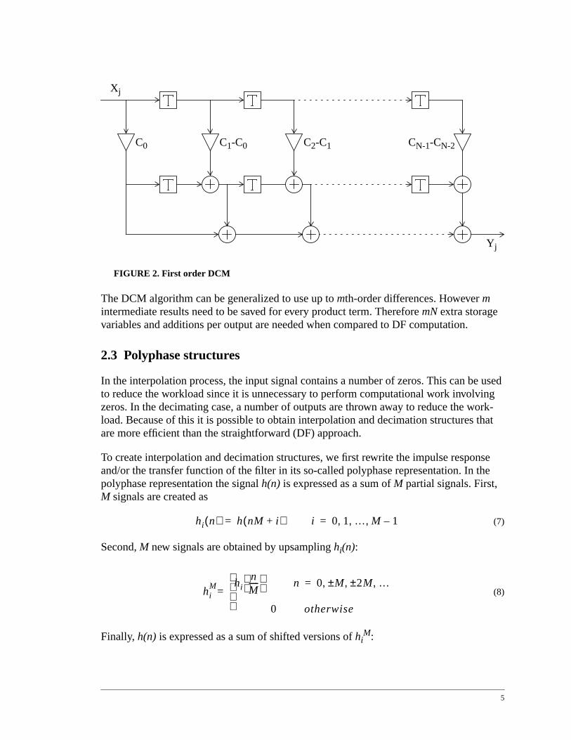
direct form computation. However, additional storage accesses and additions are reqIf the savings in multiplication are greater than the cost of extra storage access and awe have a net saving compared to DF computation.The filter structure for a first ordeDCM-filter is shown in figure 2.

CkX j k– 1+ Ck 1– Xj k– 1+ Ck Ck 1– )Xj k– 1+–(+= k 1 2 … N 1–, , ,=

Ck Ck 1– Dk1

+= k 1 2 … N 1–, , ,=

CkX j k– 1+ Ck 1– Xj k– 1+ Dk1Xj k– 1++= k 1 2 … N 1–, , ,=

Yj C0Xj C1Xj 1– … CN 1– Xj N– 1++ + +=

Yj 1+ C0Xj 1+ C1Xj … CN 1– Xj N– 2++ + +=

Yj 1+ C0Xj 1+ D11Xj( C0Xj ) … DN 1–

1Xj N– 2+( CN 2– Xj N– 2+ )+ + + + +=

4

usedingork-that

sehe

FIGURE 2. First order DCM

The DCM algorithm can be generalized to use up tomth-order differences. Howevermintermediate results need to be saved for every product term. ThereforemN extra storagevariables and additions per output are needed when compared to DF computation.

2.3 Polyphase structures

In the interpolation process, the input signal contains a number of zeros. This can beto reduce the workload since it is unnecessary to perform computational work involvzeros. In the decimating case, a number of outputs are thrown away to reduce the wload. Because of this it is possible to obtain interpolation and decimation structures are more efficient than the straightforward (DF) approach.

To create interpolation and decimation structures, we first rewrite the impulse responand/or the transfer function of the filter in its so-called polyphase representation. In tpolyphase representation the signalh(n) is expressed as a sum ofM partial signals. First,M signals are created as

(7)

Second, M new signals are obtained by upsampling hi(n):

(8)

Finally, h(n) is expressed as a sum of shifted versions ofhiM:

Xj

Yj

C0 C1-C0 C2-C1 CN-1-CN-2

hi n( ) h nM i+( )= i 0 1 … M 1–, , ,=

hiM hi

nM-----

n 0 M 2M …,±,±,=

0 otherwise

=

5

nal

(9)

(9) is the polyphase representation of the signalh(n) in the time domain.

To obtain the corresponding z-transform, we first recall that he z-transform of the sigh(n) is:

(10)

By using (10) in (9) we get

(11)

SincehiM(n) is an upsampled version ofhi(n), we have

(12)

Finally by using (12) in (11) we get:

(13)

(13) is the polyphase representation of the z-transform of the signalh(n).

2.3.1 Interpolating and decimating

The structure for a polyphase interpolating filter with a sampling rate conversion ofM isshown in figure 3.

FIGURE 3. Polyphase interpolating filter

h n( ) hiM

n i–( )i 0=

M 1–

∑=

H z( ) h n( )z n–

n 0=

∞

∑=

H z( ) hiM

n i–( )z n–

i 0=

M 1–

∑n 0=

∞

∑ hiM

n i–( )z n–

n 0=

∞

∑i 0=

M 1–

∑ …= = =

… zi–

hiM

n( )z n–z

i–Hi

Mz( )

i 0=

M 1–

∑=n 0=

∞

∑i 0=

M 1–

∑=

HiM

z( ) Hi zM( )=

H z( ) zi–Hi z

M( )i 0=

M 1–

∑=

M H(z)x(n) y(m)

fsample Mfsample

6

titys to

uta-aused thee

The polyphase representation ofH(z) is (from (13)):

(14)

By using the identity in figure 4, we get the filter structure shown in figure 5. This idenis valid because a delay ofM sampling periods at the higher sampling rate corresponda delay of one sampling period at the lower rate.

FIGURE 4. Identity

FIGURE 5. Polyphase interpolator

The filter structure in figure 5 can be simplified even more by using a so called commtor, this final filter structure is shown in figure 6. The use of a commutator works becafter the upsamplers in figure 5 only one in M sample value has a nonzero value anlower branches have a delay of 1 toM-1 sampling periods. This means, that at each timinstance at the output, only one of theM branches produces a nonzero value.

H z( ) H0 zM( ) z

1–H1 z

M( ) … zM 1–( )–

HM 1– zM( )+ + +=

MH0(zM) H0(z)Mx(n) y(m) x(n) y(m)

MH0(z)

H1(z)

HM-1(z) M

M

z-1

z-1

x(n) y(m)

7

ition

ling

F struc-

FIGURE 6. Polyphase interpolator

We can now get the structure for a polyphase decimating filter by using the transpostheorem. The filter structure is shown in figure 7 and 8.

FIGURE 7. Polyphase decimating filter

FIGURE 8. Polyphase decimator

Every subfilter H0(z) to HM-1(z) in the polyphase structure operates at the lower samprate,fsample, and the commutator operates at the higher sampling rate,Mfsample. Thismeans that the number of operations is the same for a polyphase structure and a D

H0(z)

H1(z)

HM-1(z)

x(n)

y(m)

y(Mn)

y(Mn+M-1)

M H(z)x(n) y(m)

fsampleMfsample

H0(z)

H1(z)

HM-1(z)

x(n) y(m)

fsampleMfsample

8

the

this

ptionup-ed in

ock

a-

ture, but the number of operations per second is reduced by a factor ofM in the polyphasecase.

2.4 Parallel Processing for Low-Power

The application of parallel processing to an FIR filter can increase the throughput ofFIR filter. AnL-parallel filter produces L output samples every clock cycle compared tothe original filter, which produces one output every clock cycle. However, the cost forincrease in efficiency is that if the area of the original circuit isA, then theL-parallel cir-cuit requires an area ofL*A.

It is often overlooked that the technique also can be used to reduce the power consumof an FIR filter. The application of parallel processing facilitates the lowering of the sply voltage, which leads to a decrease in the power consumption. The power consumthe original FIR filter is:

(15)

whereV0 is the supply voltage,C0 is the capacitance of the original filter andf0 is theclock frequency of the original filter. The clock frequency can be expressed as

(16)

whereT0 is the clock period of the original filter. To obtain the same sample rate, the clperiod of aL-parallel filter must be increased toLT0. This means that there is more time tocharge the capacitance, sinceC0 is charged in timeLT0, rather than in timeT0. Thisimplies that the supply voltage can be decreased toβV0, whereβ<1. The factorβ can bedetermined by examining the propagation delay of the original filter. The propagationdelay is given by

(17)

wherek is a process dependent constant andVt is the device threshold voltage. The propgation delay of the L-parallel filter is

(18)

From (EQ 17) and (EQ 18) the following equation is obtained

(19)

P0 C0V02

f 0=

f 01T0------=

Tpd

C0V0

k V0 Vt–( )α-----------------------------=

LTpd

C0βV0

k βV0 Vt–( )α---------------------------------=

L βV0 Vt–( )α β V0 Vt–( )α=

9

ely byge

ince

dershave a

This equation can be used to solveβ. Onceβ is obtained, the power consumption for theL-parallel filter can be calculated with

(20)

(20) shows that the power consumption is reduced by a factor ofβ2 when using parallelprocessing. It should be noted that the supply voltage cannot be decreased indefinitincreasing the level of parallelism in the filter. There is a lower limit on the supply voltawhich is dictated by the process parameters.

2.4.1 Fast FIR Algorithms

The polyphase representation of a traditional parallel FIR filter is

(21)

where

(22)

This implies that

(23)

These equations show that the parallel filter requiresL2 filtering operations of lengthN/L.However, it is possible to reduce the number of product terms on the RHS of (21). Sthe work of Winograd it is known that two polynomials of degreeL–1 can be multipliedusing (2L–1) product terms. By reducing the number of multipliers, the number of adincrease. Replacing multipliers with add operations is advantageous because adderssmaller implementation cost than multipliers. However, for large a number ofL the num-ber of adders becomes unmanageable.

P β2LC0( )V0

2f 0 L⁄( ) β2

C0V02

f 0= =

Yi zL( )z i–

i 0=

L 1–

∑ H j zL( )z j–

Xk zL( )z k–

k 0=

L 1–

∑j 0=

L 1–

∑=

Yi z( ) zm–

ymL i+m 0=

∞

∑= i 0 1 … L 1–, , ,=

H j z( ) zm–

hmL j+m 0=

N L⁄ 1–

∑= j 0 1 … L 1–, , ,=

Xk z( ) zm–

xmL k+m 0=

∞

∑= k 0 1 … L 1–, , ,=

Yk zL–

Hi XL k i–+ Hi Xk i–i 0=

k

∑+i k 1+=

L 1–

∑= 0 k L 2–≤ ≤

YL 1– XL 1– i–i 0=

L 1–

∑=

10

ter
Fast FIR algorithms (FFAs) use this approach to reduce the complexity of parallel filstructures. By using FFAs, theL-parallel filter can be implemented with approximately(2L–1) filtering operations of lengthN/L. The resulting parallel filter requires (2N–N/L)multipliers. For large values ofN, the advantage is clear.
2.4.2 (2-by-2) Fast FIR Algorithm

The standard 2-parallel filtering structure is

(24)

which implies that (from (23))

(25)

Figure 9 shows the resulting 2-parallel FIR filtering structure, which uses 2N multipliersand 2(N–1) additions.

FIGURE 9. Traditional 2-parallel FIR filter implementation

If we rewrite (24) we get the (2-by-2) FFA:

(26)

which implies that

Y Y0 z1–Y1+ X0 z

1–X1+( ) H0 z

1–H1+( ) …= = =

… X0H0 z1–

X0H1 X1H0+( ) z2–X1H1+ +=

Y0 H0X0 z2–H1X1+=

Y1 H0X1 H1X0+=

H0(z)

H1(z)

H0(z)

H1(z) D

x(2n)

x(2n+1)

y(2n)

y(2n+1)

Y Y0 z1–Y1+ …= =

… X0H0 z1–

X0 X1+( ) H0 H1+( ) X0H0– X1H1–[ ] z2–X1H1+ +=

11

num-

be the

(27)

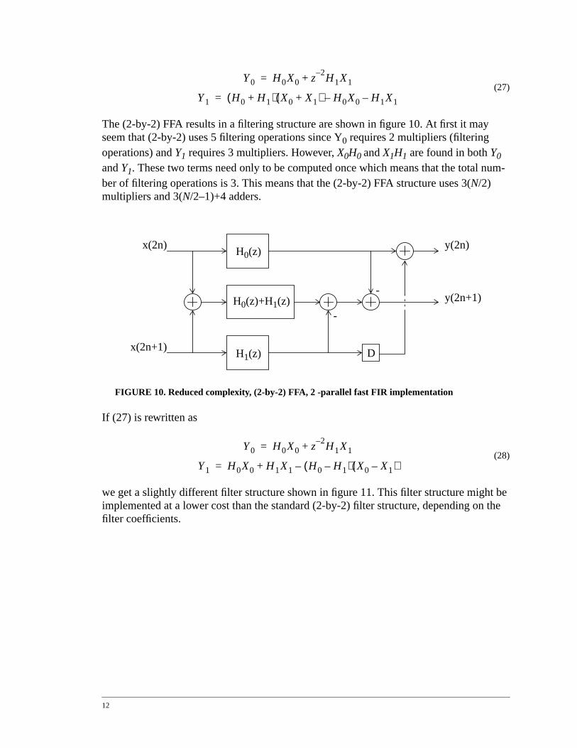
The (2-by-2) FFA results in a filtering structure are shown in figure 10. At first it mayseem that (2-by-2) uses 5 filtering operations since Y0 requires 2 multipliers (filteringoperations) andY1 requires 3 multipliers. However,X0H0 andX1H1 are found in bothY0

andY1. These two terms need only to be computed once which means that the total ber of filtering operations is 3. This means that the (2-by-2) FFA structure uses 3(N/2)multipliers and 3(N/2–1)+4 adders.

FIGURE 10. Reduced complexity, (2-by-2) FFA, 2 -parallel fast FIR implementation

If (27) is rewritten as

(28)

we get a slightly different filter structure shown in figure 11. This filter structure mightimplemented at a lower cost than the standard (2-by-2) filter structure, depending onfilter coefficients.

Y0 H0X0 z2–H1X1+=

Y1 H0 H1+( ) X0 X1+( ) H0X0– H1X1–=

H0(z)+H1(z)

H1(z)

H0(z)

D

x(2n)

x(2n+1)

y(2n)

y(2n+1)-

-

Y0 H0X0 z2–H1X1+=

Y1 H0X0 H1X1 H0 H1–( ) X0 X1–( )–+=

12

otalberut

FIGURE 11. Alternate (2-by-2) FFA

Since the implementation cost of an adder is lower than the cost of a multiplier, the tcost to implement a parallel filtering structure is approximately proportional to the numof multipliers. Based on this approximation, the cost to implement the (2-by-2) is abo25% lower, than the cost to implement a traditional 2-parallel filter structure.

H0(z)-H1(z)

H1(z)

H0(z)

D

x(2n)

x(2n+1)

y(2n)

y(2n+1)-

13

th fil-of

fileseix

nenting

3

Implementation

The FIR-filter generator is implemented in C++. The generator uses one data file witer-coefficients and different flags (-t for 2-by-2, -d for DCM etc.) to determine the typefilter that is to be implemented. The output from the FIR-filter generator are several written in VHDL-code. These files can then be compiled and syntesized to create thwanted FIR-filter. A list of all C++ files and all possible VHDL files is shown in appendB.

3.1 Input

The datafile with the filter coefficients is a normal text-file. Every line of the file has ofilter coefficient except for the first one, which has the total number of coefficients. Aexample of filter coefficients is shown in appendix C. The different options when creathe filter are shown below in table 1.

TABLE 1. Options when creating a FIR -filter.

The correct syntax for using the program is: firgen <option1> ... <optionN> filename

If an incorrect option or a non-existing filename/corrupt file is chosen, the program isstopped and an error message is shown.

Options Explanation

-c Do not include the compensation vector in the tree.

-d Use differential coefficients method (DCM).

-h Help.

-lNN Length of CSDC-vector is NN.

-pdN Use polyphase structure, decimate with M=N.

-piN Use polyphase structure, interpolate with M=N.

-s Use the symmetry of the coefficients.

-t Use 2-by-2 algorithm.

-tn Use 2-by-2 algorithm, with [H0-H1].

-wNN Input data is NN bits.

15

s N

d soo aC.

usezero

-

he

tree.fig-

First the correct number of filter coefficients is created. The number of coefficientsdepends on what type of filter that is to be implemented. For example if a DF filter usefilter coefficients then an equivalent 2-by-2 filter uses 3*N/2 coefficients. Second, the filtercoefficients are converted from string to double. Third, the coefficients are normalizethat they all are between -1 and 1. And finally, the filter coefficients are converted intstring again, but this time the string is expressed in Canonic Signed Digit Code, CSD

3.1.1 Canonic Signed Digit Code (CSDC)

An N-bit integer number,x, can be expressed as

(29)

wherexi={0,1}. The average number of nonzero bits is about half of the coefficientwordlength, i.e.N/2. It is advantageous to decrease the number of nonzero bits, becathe number of adders needed in a multiplication is proportional to the number of nonbits. One way to do so is to express the numbers in CSDC. A number,x, in the range

(30)

whereQ=2-N, N=Nd–1 forNd=odd andN=Nd–2 forNd=even is expressed in canonicsigned digit code as

(31)

wherexi={-1,0,+1} andxi*xi+1=0, i.e. no two consecutive digits are nonzero. For example, the number (11/32)10 = 0.34375 = 0.5 - 0.125 - 0.03125 = (0.10-10-1)CSDC. ForCSDC the average number of nonzero bits is

(32)

This means that for largeNd the average number of nonzero bits is about one third of tcoefficient wordlength, compared to half for binary numbers.

3.2 Filter Structure

Each filter is made of three blocks: the delay chain, the shift registers and the adderThe structure of the filter is shown in figure 12. The variables and their data types fromure 12 are listed in table 2.

x xi2i

i 0=

N 1–

∑=

4– 3⁄ Q x 4 3⁄ Q–≤ ≤+

x xi2i–

i 0=

Nd 1–

∑=

Nd

3------- 1 2

Nd–+

9--------------------+

16

Variable Data type

clk std_logic

indata std_logic_vector

from_delay_array std_logic_array_delay

to_shift_n std_logic_vector

shift_array_n std_logic_array_shift

outdata std_logic_vectorTABLE 2. Variables and their data types

17

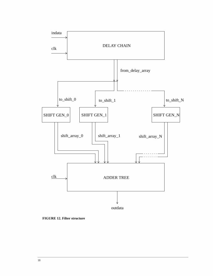
FIGURE 12. Filter structure

indata

clkDELAY CHAIN

SHIFT GEN_0 SHIFT GEN_1 SHIFT GEN_N

from_delay_array

to_shift_0 to_shift_Nto_shift_1

ADDER TREE

shift_array_Nshift_array_0 shift_array_1

clk

outdata

18

filterains

or.ely.

aved vec-

e firstlti-ally0.25

n thera extra

idth vec-

tor.ossi-

madeeated.er ofmple

Each filter is created in four steps:

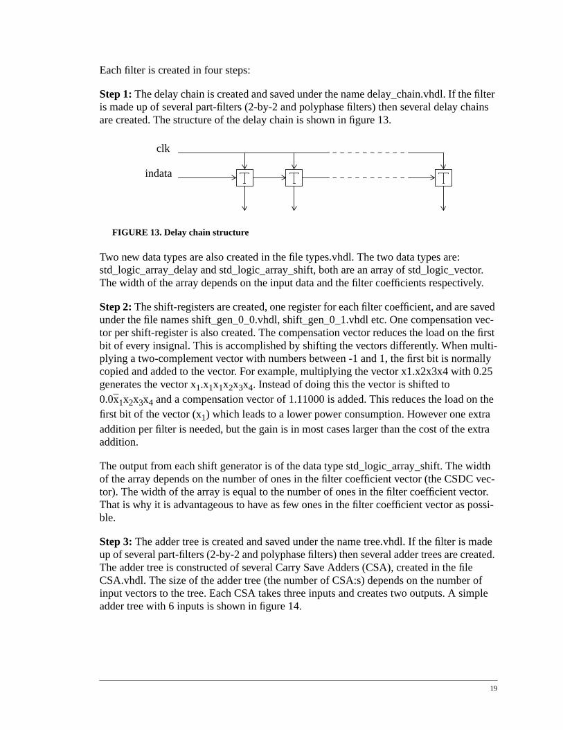
Step 1:The delay chain is created and saved under the name delay_chain.vhdl. If theis made up of several part-filters (2-by-2 and polyphase filters) then several delay chare created. The structure of the delay chain is shown in figure 13.

FIGURE 13. Delay chain structure

Two new data types are also created in the file types.vhdl. The two data types are:std_logic_array_delay and std_logic_array_shift, both are an array of std_logic_vectThe width of the array depends on the input data and the filter coefficients respectiv

Step 2:The shift-registers are created, one register for each filter coefficient, and are sunder the file names shift_gen_0_0.vhdl, shift_gen_0_1.vhdl etc. One compensationtor per shift-register is also created. The compensation vector reduces the load on thbit of every insignal. This is accomplished by shifting the vectors differently. When muplying a two-complement vector with numbers between -1 and 1, the first bit is normcopied and added to the vector. For example, multiplying the vector x1.x2x3x4 with generates the vector x1.x1x1x2x3x4. Instead of doing this the vector is shifted to0.0x1x2x3x4 and a compensation vector of 1.11000 is added. This reduces the load ofirst bit of the vector (x1) which leads to a lower power consumption. However one extaddition per filter is needed, but the gain is in most cases larger than the cost of theaddition.

The output from each shift generator is of the data type std_logic_array_shift. The wof the array depends on the number of ones in the filter coefficient vector (the CSDCtor). The width of the array is equal to the number of ones in the filter coefficient vecThat is why it is advantageous to have as few ones in the filter coefficient vector as pble.

Step 3: The adder tree is created and saved under the name tree.vhdl. If the filter is up of several part-filters (2-by-2 and polyphase filters) then several adder trees are crThe adder tree is constructed of several Carry Save Adders (CSA), created in the filCSA.vhdl. The size of the adder tree (the number of CSA:s) depends on the numbeinput vectors to the tree. Each CSA takes three inputs and creates two outputs. A siadder tree with 6 inputs is shown in figure 14.

clk

indata

19

also

derle-creat-dl.

nderec-

FIGURE 14. Carry Save Adder tree

The adder tree for the DCM filter looks a little different because delay elements are included in the tree. The structure of the DCM filter is shown in figure 2.

Step 4: The final step is to connect the delay chain with the shift registers and the adtree. This is done in the file connect.vhdl. Additional adders, subtracters and delay ements are connected for 2-by-2 filters, this is done in the file tbtconnect.vhdl. When ing polyphase filters the different part-filters are connected in the file polyconnect.vh

Finally the program writes out the name of the VHDL-file with the highest hierachy athe name of the input- and output variables. This is done to simplify things for the uswhen he simulates the filter in ModelSim and later when synthesizing in LeonardoSptrum.

In appendix B there is a list of all possible VHDL-files that can be created.

CSA CSA

CSA

CSA

20

andpared

lterst if

38 fil-is is

4

Simulation

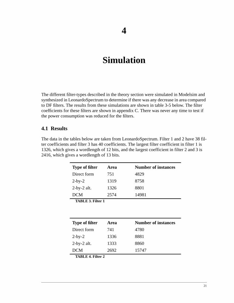
The different filter-types described in the theory section were simulated in Modelsimsynthesized in LeonardoSpectrum to determine if there was any decrease in area comto DF filters. The results from these simulations are shown in table 3-5 below. The ficoefficients for these filters are shown in appendix C. There was never any time to tethe power consumption was reduced for the filters.

4.1 Results

The data in the tables below are taken from LeonardoSpectrum. Filter 1 and 2 haveter coefficients and filter 3 has 40 coefficients. The largest filter coefficient in filter 1 1326, which gives a wordlength of 12 bits, and the largest coefficient in filter 2 and 32416, which gives a wordlength of 13 bits.

Type of filter Area Number of instances

Direct form 751 4829

2-by-2 1319 8758

2-by-2 alt. 1326 8801

DCM 2574 14981TABLE 3. Filter 1



2-by-2 1336 8881

2-by-2 alt. 1333 8860


21

lters coef-d for

F fil-by-2ruc-

noth-ality

h hap-lter

4.2 Conclusions

The DCM filters are not even close to be any better than the DF filters. However the fitested in this case are not specifically designed to be implemented with the differentficients method. No real conclusions can be drawn before a filter specifically designeDCM is tested.

The area for a 2-parallel filter is approximately two times larger than the area for a Dter. 2-by-2 filters use less than two times the area for the DF filters. Therefore the 2-algorithm seems to be an improvement compared to the traditional 2-parallel filter stture.

The polyphase filter structure was simulated and synthesized, too, but since there ising to compare these filters to, the simulations were only made to confirm the functionof the program.

One interesting result with the DF filters is that even if the filter coefficient wordlengtwas increased from 12 in filter 1 to 13 in filter 2 the area decreased. The same thingpened when the number of filter coefficients was increased from 38 in filter 2 to 40 in fi3. This shows how difficult it can be to design efficient FIR filters.



2-by-2 1330 8754

2-by-2 alt. 1309 8577


22

s

s-

References[1] Jan Skansholm:C++ direkt, Studentlitteratur, 1996.

[2] Lars Wanhammar and Håkan Jonasson: Digital filters, Department of Electri-cal Engineering, Linköping University, 2000.

[3] Lars Wanhammar: DSP Integrated Circuits, Academic press, 1999.

[4] James R. Armstrong and F. Gail Gray: VHDL Design, Representation andSynthesis, second edition, Prentice Hall PTR, 2000.

[5] N. Sankarayya, Kaushik Roy and Debashis Bhattacharya:Algorithms for LowPower and High Speed FIR Filter Realization Using Differential Coefficient,IEEE Trans. Circuit Syst. II, vol 47, pp. 488-496, June 1997.

[6] Tian-Sheuan Chang, Yuan-Hua Chu and Chein-Wei Jen:Low-Power FIR Fil-ter Realization with Differentail Coefficients and Inputs, IEEE Trans. CircuitSyst. II, vol 47, Feb. 2000.

[7] David A. Parker and Keshab K. Parhi:Area-Efficient Parallel FIR Digital Fil-ter Implementations, Application Specific Systems, Architectures and Procesors, 1996.

[8] Mentor Graphics. www.mentor.com

23

Appendix Alibrary ieee;

use ieee.std_logic_1164.all;

use WORK.types.all;

entity DELAY_CHAIN_0 is

port (a : in std_logic_vector((12-1) downto 0);

y : out std_logic_array_delay;

clk: in std_logic);

end DELAY_CHAIN_0;

architecture STRUCTURAL of DELAY_CHAIN_0 is

signal store : std_logic_array_delay;

begin

store(0) <= a;

storage: process (clk)

begin

if clk’event and clk = ’1’ then

store(11-1 downto 1) <= store((11-2) downto 0);

end if;

end process storage;

y <= store;

end STRUCTURAL;

25

Appendix B

List of C++ files

• adder.cpp

• connect.cpp

• conversions.cpp

• csagen.cpp

• dcmtreegen.cpp

• delay.cpp

• delaychain.cpp

• firgen.cpp

• polyconnect.cpp

• shiftgen.cpp

• symmetryadders.cpp

• tbtadder.cpp

• tbtconnect.cpp

• tbtsubtracter.cpp

• treegen.cpp

• types.cpp

List of VHDL-files that can be generated

• connect.vhdl

• CSA_N.vhdl

• CSS_N.vhdl

• dcmtree_n.vhdl

• delay.vhdl

• delay_chain_n.vhdl

• polyconnect.vhdl

• shift_gen_n_m.vhdl

• tbtadder.vhdl

• tbtconnect.vhdl

• tree_n.vhdl

• types.vhdl

27

Appendix CFilter 1 Filter 2 Filter 3

-2 -2 -1

0 0 -2

5 10 0

5 9 10

-7 -14 8

-17 -32 -14

0 0 -32

32 60 0

27 48 60

-34 -64 48

-72 -133 -64

0 0 -132

120 220 0

96 176 220

-127 -232 176

-280 -512 -232

0 0 -512

704 1284 0

1326 2416 1284

1326 2416 2416

704 1284 2416

0 0 1284

-280 -512 0

-127 -232 -512

96 176 -232

120 220 176

0 0 220

-72 -133 0

-34 -64 -132

27 48 -64

32 60 48

0 0 60

-17 -32 0

-7 -14 -32

5 9 -14

5 10 8

0 0 10

-2 -2 0

-2

-1

29

30

På svenska

Detta dokument hålls tillgängligt på Internet – eller dess framtida ersättare – under en län-gre tid från publiceringsdatum under förutsättning att inga extra-ordinära omständigheteruppstår.

Tillgång till dokumentet innebär tillstånd för var och en att läsa, ladda ner, skriva ut ens-taka kopior för enskilt bruk och att använda det oförändrat för ickekommersiell forskningoch för undervisning. Överföring av upphovsrätten vid en senare tidpunkt kan inteupphäva detta tillstånd. All annan användning av dokumentet kräver upphovsmannensmedgivande. För att garantera äktheten, säkerheten och tillgängligheten finns det lösningarav teknisk och administrativ art.

Upphovsmannens ideella rätt innefattar rätt att bli nämnd som upphovsman i den omfatt-ning som god sed kräver vid användning av dokumentet på ovan beskrivna sätt samt skyddmot att dokumentet ändras eller presenteras i sådan form eller i sådant sammanhang somär kränkande för upphovsmannens litterära eller konstnärliga anseende eller egenart.

För ytterligare information om Linköping University Electronic Press se för-lagets hemsidahttp://www.ep.liu.se/

In English

The publishers will keep this document online on the Internet - or its possible replacement- for a considerable time from the date of publication barring exceptional circumstances.

The online availability of the document implies a permanent permission for anyone toread, to download, to print out single copies for your own use and to use it unchanged forany non-commercial research and educational purpose. Subsequent transfers of copyrightcannot revoke this permission. All other uses of the document are conditional on the con-sent of the copyright owner. The publisher has taken technical and administrative mea-sures to assure authenticity, security and accessibility.

According to intellectual property law the author has the right to be mentioned when his/her work is accessed as described above and to be protected against infringement.

For additional information about the Linköping University Electronic Press and its proce-dures for publication and for assurance of document integrity, please refer to its WWWhome page: http://www.ep.liu.se/

© [Michael Broddfelt]

design of a finite-impulse response filter generator19355/fulltext01.pdf · design of a...

Documents