design methods for control systems - dynamics and … institute of systems and control steady-state...

Dutch Institute of Systems and Control

Chapter 2

Classical Control SystemDesign


Steady-state errorsSteady-state errors

Type k systemsType k systems

Integral controlIntegral control

Frequency response plotsFrequency response plots

Bode plotsBode plots

Nyquist plotsNyquist plots

Nichols plotsNichols plots

Classical design specificationsClassical design specifications

Lead, lag, lead-lag compensationLead, lag, lead-lag compensation

Quantitative Feedback TheoryQuantitative Feedback Theory

IntroductionIntroduction Classical design techniquesClassical design techniques

Ch. 2. Classical control system designCh. 2. Classical control system design

M- and N-circlesM- and N-circles

Guillemin-Truxal methodGuillemin-Truxal method

Root locusRoot locus

Overview


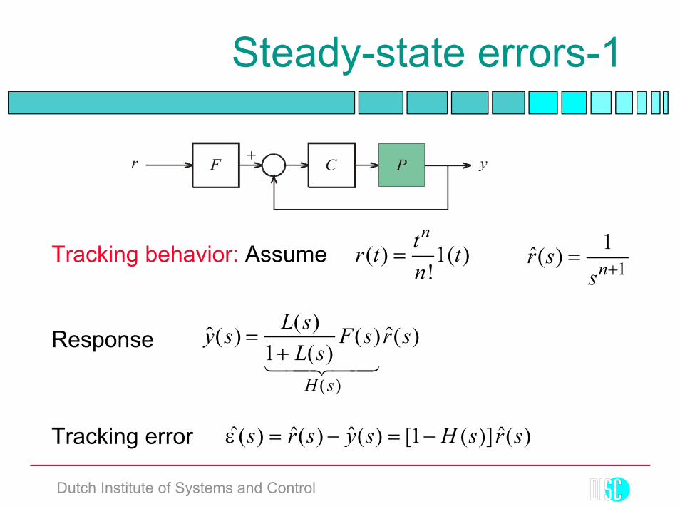
Steady-state errors-1

Tracking behavior: Assume

Tracking error

r yF C P+

−

( ) 1( )!

ntr t tn

=1

1ˆ( ) nr ss +

=

$( ) ( )( )

( ) $( )

( )

y s L sL s

F s r s

H s

=+11 244 344

Response

ˆ ˆ ˆ ˆ( ) ( ) ( ) [1 ( )] ( )s r s y s H s r sε = − = −



Steady-state tracking error

If F(s)=1 (no prefilter) then

( )0 0

1 ( )ˆlim ( ) lim ( ) limnnt s s

H st s ss

ε ε ε∞→∞ → →

−= = =

( )0

1lim[1 ( )]

nns s L s

ε∞→

=+

11 ( )1 ( )

H sL s

− =+


Type k system

A feedback system is of type k if

Then

( )( ) , (0) 0o

okL s

L s Ls

= ≠

( )

0

0

1lim[1 ( )]

0 for 0lim 1/ (0) for

( )for

nns

k n

okso

s L sn k

s L n ks L s

n k

ε∞ →

−

→

=+

≤ <= = =+ ∞ >


Integral control-1

Integral control:Design the closed-loop system such that

Type k control:

Results in good steady-state behavior

Also:

( )( ) oL s

L ss

=

( )( ) o

kL s

L ss

=

1( ) ( ) for 01 ( ) ( )

kk

ko

sS s s sL s s L s

= = = →+ +

O


Integral control-2

then the steady-state error is zero if n < k (rejection)

Hence if

( ) ( ) for 0kS s s s= →O

11ˆ( ) 1 ( ), ( )

!

n

ntv t t v sn s +

= =

k = 1: Integral control: Rejection of constant disturbancesk = 2: Type-2 control: Rejection of ramp disturbancesEtc.

Type k control:


Integral control-3

Integral control:

“Natural” integrating action is present if the plant transferfunction has one or several poles at 0

If no natural integrating action exists then the compen-sator needs to provide it

The loop has integrating action of order k

( )( ) ( ) ( )o

kL s

L s P s C ss

= =


Integral control-4

“Pure” integral control: 1( )i

C ssT

=

1( ) 1i

C s gsT

= +

1( ) 1di

C s g sTsT

= + +

PI control:

PID control:

Ziegler-Nichols tuning rules


Internal model principle

Asymptotic tracking if model of disturbance is included inthe compensator

Francis, D.A. and Wonham, W.M., (1975) The internal model principle forlinear multivariable regulators, Applied Mathematics and Optimization, vol 2,pp. 170-194


Frequency response plots

Bode plots Nichols plots

Nyquist

plots


Bode plots-1

2

2 2( )( ) 2 ( )

o

o o oL j

j jω

ωω ζ ω ω ω

=+ +

Bode plot:doubly logarithmicplot of |L(jω)| versusωsemi logarithmic plotof arg L(jω) versus ω


Bode plots-2

Helpful technique:

By construction of the asymptotic Bode plots ofelementary first- and second-order factors of the form

1 2

1 2

( )( ) ( )( )

( )( ) ( )m

m

j z j z j zL j k

j p j p j pω ω ω

ωω ω ω

− − −=

− − −L

L

The shape of the Bode plot of

2 2 20( ) 2 ( )o oj j jω α ω ζ ω ω ω+ + +and

may be sketched


Nyquist plots

Nyquist plot: Locus ofL(jω) in the complex planewith ω as parameterContains less informationthan the Bode plot if ω isnot marked along thelocus

2

2 2( )( ) 2 ( )

o

o o oL j

j jω

ωω ζ ω ω ω

=+ +


M- and N-circles-1

M-circle: Locus of points z in the complex plane where

Closed-loop transfer function:

N-circle: Locus of points z in the complex plane where

H LL

T=+

=1

zz

M1+

=

arg zz

N1+

=

L−

r y+


M- and N-circles-2


Nichols plots

Nichols plot: Locus ofL(jω) with ω as para-meter in the

log magnitudeversus

argumentplane

Nichols chart: Nichols plotwith M- and N-lociincluded

2

2 2( )( ) 2 ( )

o

o o oL j

j jω

ωω ζ ω ω ω

=+ +


Time

domain

Freq

uenc

ydo

mainBandwidth,resonance peak,roll-on and roll-off ofthe closed-loopfrequency responseand sensitivityfunctions; stabilitymargins

Rise time, delay time,overshoot, settling time,steady-state error of theresponse to stepreference anddisturbance inputs;error constants

Classical design specifications


Classical design techniques

Lead, lag, and lag-lead compensation (loopshaping)(Root locus approach)(Guillemin-Truxal design procedure)Quantitative feedback theory QFT (robust loopshaping)


Classical design techniques

Change open-loop L(s) to achieve certain closed-loop specsfirst modify phasethen correct gain

Rules for loopshaping


Lead compensation

Lead compensation:Add extra phase in thecross-over region toimprove the stabilitymarginsTypical compensator:“Phase-advancenetwork”

1( ) , 0 11

j TC jj Tω

ω α αωα

+= < <

+


Lead/lag compensator

1( )1

j TC jj Tω

ω αωα

+=

+


Lag compensation

Lag compensation:Increase the low frequency gain without affecting thephase in the cross-over region

Example: PI-control:

1( ) j TC j kj Tω

ωω

+=


Lead-lag compensation

Lead-lag compensation: Joint use oflag compensation at low frequenciesphase lead compensation at crossover

Lead, lag, and lead-lag compensation are always usedin combination with gain adjustment


Notch compensation

(inverse) Notch filters:

suppression of parasitic dynamicsadditional gain at specific frequencies

Special form of general second order filter


Notch compensation

12

12

222

2

21

121

2

++

++==

ωβ

ω

ωβ

ωε ss

ssuH

“Notch”-filter :ω1= ω2


Notch compensation

ampl.

fase

2

1

ββ

0°


Root locus method-1

Important stage of many designs: Fine tuning of

gaincompensator pole and zero locations

Helpful approach: the root locus method (use rltool!)


Root locus method-2

Closed-loop characteristic polynomial

Root locus method: Determine the loci of the roots of χ asthe gain k varies

1 2

1 2

( )( ) ( )( )( )( ) ( )( ) ( )

m

n

s z s z s zN sL s kD s s p s p s p

− − −= =

− − −L

L

1 2 1 2

( ) ( ) ( )( )( ) ( ) ( )( ) ( )n m

s D s N ss p s p s p k s z s z s z

χ = += − − − + − − −L L

L−


Root locus method-3

Rules:For k = 0 the roots are the open-loop poles piFor k → ∝ a number m of the roots approach theopen-loop zeros zi. The remaining roots approach ∝The directions of the asymptotes of those roots thatapproach ∝ are given by the angles

1 2 1 2( ) ( )( ) ( ) ( )( ) ( )n ms s p s p s p k s z s z s zχ = − − − + − − −L L

2 1 , 0, 1, , 1i i n mn m

π+

= − −−

L


Root locus method-4

The asymptotes intersect on the real axis in the point

Those sections of the real axis located to the left ofan odd total number of open-loop poles and zeros onthis axis belong to a locusThe loci are symmetric with respect to the real axis....

(sum of open-loop poles) (sum of open-loop zeros)n m−−


Root locus method-5

( )( 2)

kL ss s

=+

( 2)( )( 1)

k sL ss s

+=

+( )

( 1)( 2)kL s

s s s=

+ +


Guillemin-Truxal method-1

Procedure:Specify HSolve the compensator from

Closed-loop transferfunction:

1PCH

PC=

+

11

HCP H

= ⋅−

C P−

+

yr



Example: Choose

This guarantees the system to be of type m + 1

11 0

1 11 1 0

( )m m

m mn n m m

n m m

a s a s aH s

s a s a s a s a

−−

− −− −

+ + +=

+ + + + + +

L

L L

How to choose the denominator polynomial?Well-known options:

Butterworth polynomialsOptimal ITAE polynomials


Butterworth and ITAE polynomials

Butterworth polynomialsChoose the n left-half plane poles on the unit circle sothat together with their right-half plane mirror imagesthey are uniformly distributed along the unit circle

ITAE polynomialsPlace the poles so that

is minimal, where e is the tracking error for a step input

0( )t e t dt

∞

∫


Butterworth and ITAE

0m =



Disadvantages of the method:Difficult to translate the specs into an unambiguouschoice of H. Often experimentation with other designmethods is needed to establish what may beachieved. In any case preparatory analysis isrequired to determine the order of the compensatorand to make sure that it is properThe method often results in undesired pole-zerocancellation between the plant and the compensator


Quantitative feedback theory QFT-1

Ingredients of QFT:For a number of selected frequencies, represent theuncertainty regions of the plant frequency responsein the Nichols chartSpecify tolerance bounds on the magnitude of TShape the loop gain so that the tolerance boundsare never violated


QFT-2

Example: Plant

Parameter uncertainties:

Nominal parameter values:

Tentative compensator:

2( )(1 )

gP ss sθ

=+

1, 0g θ= =

( ) , 1, 1.414, 0.11

dd o

o

k sTC s k T T

sT+

= = = =+

0.5 2, 0 0.2g θ≤ ≤ ≤ ≤


QFT-3

Responses of the nominal design

Specs on |T |

Frequency[rad/s]

0.212510

Tolerance band[dB]

0.5251020


Uncertainty regions

Uncertaintyregions for thenominal designThe specs arenot satisfiedAdditionalrequirement:The critical areamay not beentered


QFT-4

Design method: Manipulate the compensator frequencyreponse so that the loop gainsatisfies the tolerance boundsavoids the critical region

Preparatory step 1: For each selected frequency,determine the performance boundaryPreparatory step 2: For each selectedfrequency,determine the robustness boundary


Performance and robustness boundaries

Nominal plantfrequencyresponse

Robustnessboundaries

Performanceboundaries


QFT-5

Design step: Modify the loop gain such that for eachselected frequency the corresponding point on the loopgain plot lies above and to the right of the correspondingboundaryFor the case at hand this may be accomplished by a leadcompensator of the form

1

2

1( )1

sTC ssT

+=

+

Step 1: Set T2 = 0, vary T1

Step 2: Keep T1 fixed, vary T2


QFT-6

Eventualdesign:T1 = 3T2 = 0.02


QFT-7

Responses of theredesigned system


cl ( ) 0.02 ( 2.7995)(( 46.8190.38 0)( ) 1

15)D s s ss

sN

= ++ +=

Prefilter design-1

2½-degree-of-freedomconfigurationClosed-loop transferfunction

For the present case:

H NFD

Fo=cl

P− +

+

r

zu

Y

F

X

X

Co

e

Fo


Prefilter design-2

Use the polynomial F to cancel the (slow) pole at –0.3815,and let

Perturbedresponses

F ss so

o

o o oo o( ) , ,=

+ += =

ω

ζ ω ωω ζ

2

2 2122

1 2

design methods for control systems - dynamics and … institute of systems and control steady-state...

Documents