design methodology of an axial flow turbine for a micro

Design methodology of an axial-

flow turbine for a micro jet engine

by

Johan George Theron Basson

Thesis presented in partial fulfilment of the requirements for the degree of

Master of Science in Engineering (Mechanical)

in the Faculty of Engineering at

Stellenbosch University

Supervisor: Prof. T.W. von Backström

Co-supervisor: Dr S.J. van der Spuy

December 2014

i

DECLARATION

By submitting this thesis electronically, I declare that the entirety of the work

contained therein is my own, original work, that I am the sole author thereof (save

to the extent explicitly otherwise stated), that reproduction and publication thereof

by Stellenbosch University will not infringe any third party rights and that I have

not previously in its entirety or in part submitted it for obtaining any qualification.

Date: ...............................................

Copyright © 2014 Stellenbosch University

All rights reserved

Stellenbosch University http://scholar.sun.ac.za

ii

Abstract

Design methodology of an axial-flow turbine for a micro jet engine

J.G.T. Basson

Department of Mechanical and Mechatronic Engineering, Stellenbosch

University,

Private Bag X1, Matieland 7602, South Africa

Thesis: MEng. (Mechanical)

December 2014

The main components of a micro gas turbine engine are a centrifugal or mixed-

flow compressor, a combustion chamber and a single stage axial-flow or radial-

flow turbine. The goal of this thesis is to formulate a design methodology for

small axial-flow turbines. This goal is pursued by developing five design-related

capabilities and applying them to develop a turbine for an existing micro gas

turbine engine. Firstly, a reverse engineering procedure for producing digital

three-dimensional models of existing turbines is developed. Secondly, a procedure

for generating candidate turbine designs from performance requirement

information is presented. The third capability is to use independent analysis

procedures to analyse the performance of a turbine design. The fourth capability is

to perform structural analysis to investigate the behavior of a turbine design under

static and dynamic loading. Lastly, a manufacturing process for prototypes of a

feasible turbine design is developed. The reverse engineering procedure employs

point cloud data from a coordinate measuring machine and a CT-scanner to

generate a three-dimensional model of the turbine in an existing micro gas turbine

engine. The design generation capability is used to design three new turbines to

match the performance of the turbine in the existing micro gas turbine engine.

Independent empirical and numerical turbine performance analysis procedures are

developed. They are applied to the four turbine designs and, for the new turbine

designs, the predicted efficiency values differ by less than 5% between the two

procedures. A finite element analysis is used to show that the stresses in the roots

of the turbine rotor blades are sufficiently low and that the dominant excitation

frequencies do not approach any of the blade natural frequencies. Finally

prototypes of the three new turbine designs are manufactured through an

investment casting process. Patterns made of an organic wax-like material and a

polystyrene material are used, with the former yielding superior results.


iii

Opsomming

'n Ontwerpsmetodologie van ‘n aksiaalvloei-turbine vir ‘n mikro-

gasturbiene-enjin

J.G.T. Basson

Departement van Meganiese en Megatroniese Ingenieurswese, Universiteit van

Stellenbosch,

Privaatsak X1, Matieland 7602, Suid-Afrika

Tesis: MIng. (Meganies)

Desember 2014

Mikro-gasturbiene-enjins bestaan uit 'n sentrifugaal- of ‘n gemende-

vloeikompressor, 'n verbrandingsruim en 'n enkel-stadium-aksiaalvloei- of ‘n

radiaalvloei-turbine. Die doel van hierdie tesis is om 'n ontwerpsmetodologie vir

klein aksiaalvloei-turbines saam te stel. Hierdie doel word deur die ontwikkeling

en toepassing van vyf ontwerpsverwante vermoëns nagestreef. Eerstens word 'n

tru-waartse-ingenieursproses ontwikkel om drie-dimensionele rekenaarmodelle

van die bestaande turbines te skep. Tweedens word 'n metode om

kandidaatturbineontwerpe vanaf werkverrigtingsvereistes te verkry, voorgestel.

Die derde ontwerpsvermoë is om die werksverrigting van 'n turbineontwerp met

onafhanklike analises te evalueer. Die vierde ontwerpsvermoë is om die struktuur

van 'n turbinelem te analiseer sodat die effek van statiese en dinamiese belastings

ondersoek kan word. Laastens word 'n vervaardigingsproses vir prototipes van

geskikte turbineontwerpe ontwikkel. Die tru-waartse-ingenieursproses maak

gebruik van 'n koördinaat-meet-masjien en 'n CT-skandeerder om puntewolkdata

vanaf die turbine in 'n bestaande mikro-gasturbiene-enjin te verkry. Die data word

dan gebruik om 'n drie-dimensionele model van die turbine te skep. Die

ontwerpskeppingsvermoë word dan gebruik om drie kandidaatturbineontwerpe vir

die bestaande mikro-gasturbiene-enjin te skep. Onafhanklike empiriese en

numeriese prosedures om die werkverrigting van 'n turbineontwerp te analiseer

word ontwikkel. Beide prosedures word op die vier turbineontwerpe toegepas.

Daar word gevind dat die voorspelde benuttingsgraadwaardes van die nuwe

ontwerpe met minder as 5% verskil vir die twee prosedures. 'n Eindige-element-

analise word dan gebruik om te wys dat die spannings in die wortels van die

turbinelemme laag genoeg is, asook dat die dominante opwekkingsfrekwensies

nie die lem se natuurlike frekwensies nader nie. Laastens word prototipes van die

drie nuwe turbineontwerpe deur 'n beleggingsgietproses vervaardig. In die

vervaardigingproses word die effektiwiteit van twee materiale vir die gietpatrone


iv

getoets, naamlik 'n organiese wasagtige materiaal en 'n polistireen-materiaal. Daar

word bevind dat die gebruik van die wasagtige gietpatrone tot beter resultate lei.


v

Acknowledgements

I would not have completed this project had it not been for certain people.

My Lord and Savior Jesus Christ, for the peace and hope I have in Him.

My father, Anton, who has always set an example and never has shied away from

telling me what I need to hear.

My mother, Erina. Your willing company and unconditional support has always

kept me confident and positive.

My friends and family. You have supported me and kept me interested throughout

the duration of my studies.

My supervisors: Prof. T.W. von Backström for his patience and interesting stories

and Dr. S.J. van der Spuy for optimism and guidance.

My wife, Elsje. Going home to you is what I look forward to at the end of every

day.


vi

To my parents


vii

Table of contents

DECLARATION ...................................................................................................... i

Abstract ................................................................................................................... ii

Opsomming ............................................................................................................ iii

Acknowledgements .................................................................................................. v

Table of contents ................................................................................................... vii

List of figures ........................................................................................................... x

List of tables .......................................................................................................... xii

Nomenclature ....................................................................................................... xiii

1. Introduction ...................................................................................................... 1

1.1. Background and motivation ......................................................................... 1

1.2. Objectives .................................................................................................... 2

1.3. Overview of the thesis ................................................................................. 3

1.4. A note on turbine blade and flow angle conventions ................................... 4

2. Reverse engineering an existing turbine .......................................................... 7

2.1. Introduction .................................................................................................. 7

2.2. Component point cloud extraction ............................................................... 7

2.3. Processing raw point coordinate data ........................................................ 12

2.4. Three-dimensional model reconstruction .................................................. 15

2.5. Conclusion ................................................................................................. 16

3. Performance analysis using an empirical loss model .................................... 17

3.1. Introduction ................................................................................................ 17

3.2. Empirical loss model ................................................................................. 17

3.3. Performance analysis procedure ................................................................ 28

3.4. Results of empirical performance analysis ................................................ 32

3.5. Conclusion ................................................................................................. 33

4. Turbine design process .................................................................................. 35

4.1. Introduction ................................................................................................ 35

4.2. Assumptions and design decisions ............................................................ 35

4.3. Design parameters ...................................................................................... 37

4.4. Mean radius gas velocity triangles and efficiency estimate ...................... 41

4.5. Gas states calculation ................................................................................. 43

4.6. Flow path annulus sizing ........................................................................... 44

4.7. Blade profile construction .......................................................................... 45

4.8. Empirical performance analysis ................................................................. 50


viii

4.9. Root-to-tip blade design ............................................................................. 51

4.10. Conclusion ................................................................................................. 53

5. CFD performance analysis of turbine stage ................................................... 54

5.1. Introduction ................................................................................................ 54

5.2. Physical conditions simulated .................................................................... 54

5.3. CFD methodology ...................................................................................... 54

5.4. CFD performance analysis ......................................................................... 57

5.5. Conclusion ................................................................................................. 62

6. FEM structural analysis of turbine rotor ........................................................ 63

6.1. Introduction ................................................................................................ 63

6.2. Physical conditions simulated .................................................................... 63

6.3. FE modelling of the physical problem ....................................................... 63

6.4. Static structural analysis ............................................................................ 66

6.5. Modal analysis ........................................................................................... 67

6.6. Conclusion ................................................................................................. 70

7. Turbine prototype manufacturing process ..................................................... 71

7.1. Introduction ................................................................................................ 71

7.2. Material selection ....................................................................................... 71

7.3. Required final component geometries ....................................................... 71

7.4. Modification of desired final component geometries ................................ 72

7.5. Pattern creation .......................................................................................... 73

7.6. Investment casting process ........................................................................ 74

7.7. Investment casting results .......................................................................... 75

7.8. Conclusion ................................................................................................. 77

8. Conclusion ..................................................................................................... 78

8.1. Development and implementation of the design methodology ................. 78

8.2. Suggestions for future research .................................................................. 80

Appendix A: Empirical performance model calculations ...................................... 81

A.1. BMT 120 KS turbine stator blade row total pressure loss coefficient

sample calculation .................................................................................................. 81

A.2. Exit static pressure based state solution sample calculations .................... 86

Appendix B: Turbine design process calculations ................................................. 91

B.1. Turbine inlet total temperature sample calculation .................................... 92

B.2. Non-dimensional performance parameters sample calculation ................. 93

B.3. Mean radius gas velocity triangle calculations .......................................... 94

B.4. Turbine gas states sample calculation ........................................................ 95

B.5. Blade row geometric parameters – sample calculations ............................ 99

Appendix C: CFD verification ............................................................................. 102


ix

C.1. Inlet and outlet block length independence ............................................. 102

C.2. Computational mesh independence ......................................................... 102

Appendix D: FEM analysis information .............................................................. 104

D.1. Material properties of Inconel IN713 LC ................................................ 104

D.2. FEM mesh convergence studies .............................................................. 104

References ............................................................................................................ 106


x

List of figures

Figure 1-1: Consistent blade and flow angle convention ........................................ 5

Figure 1-2: Generic blade angle convention ............................................................ 5

Figure 2-1: Mitutoyo Bright Apex 710 ..................................................................... 8

Figure 2-2: CMM turbine rotor configuration ......................................................... 9

Figure 2-3: CMM measurement paths on the turbine rotor wheel ........................ 10

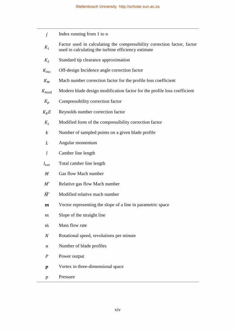
Figure 2-4: Phoenix v|tome|x m high resolution CT-scanner ................................ 11

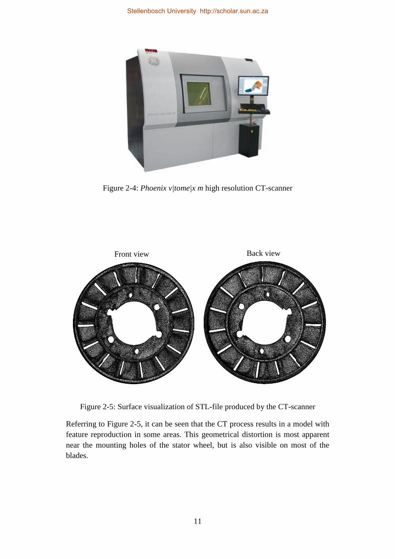
Figure 2-5: Surface visualization of STL-file produced by the CT-scanner ......... 11

Figure 2-6: Blade profile curve section divisions .................................................. 13

Figure 2-7: LE curve section point sampling ......................................................... 14

Figure 2-8: Three-dimensional turbine stator and rotor wheel reconstructions ..... 16

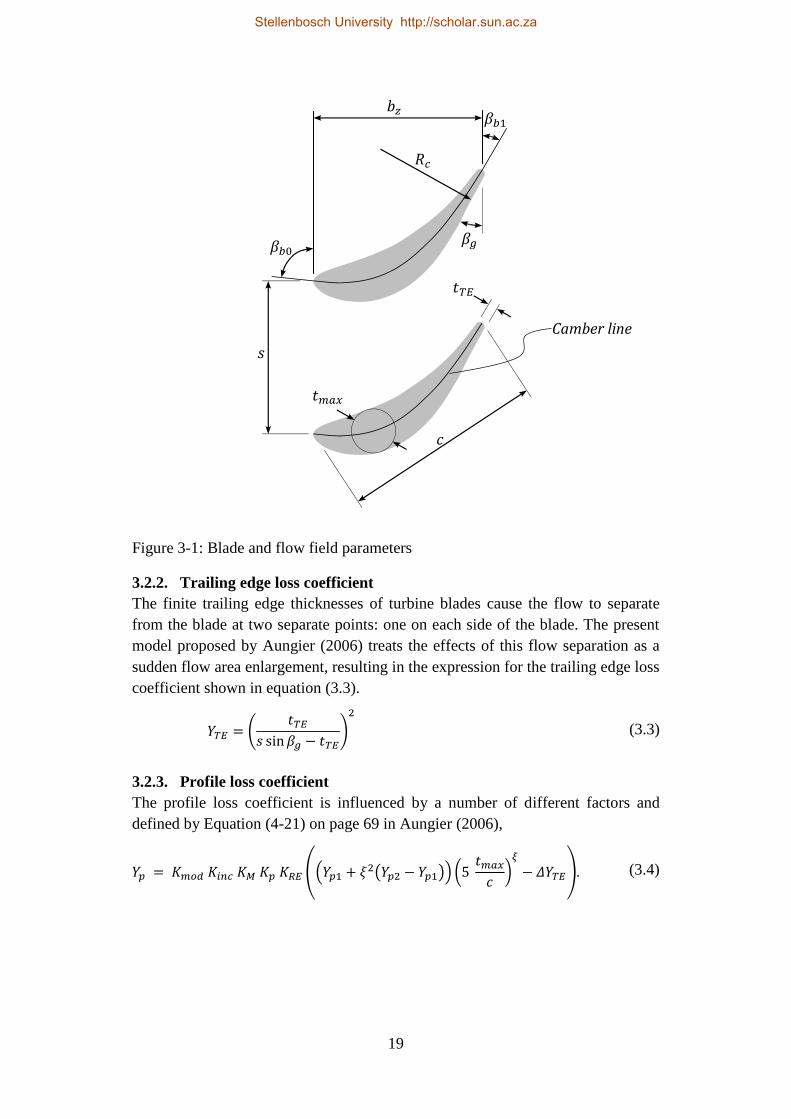
Figure 3-1: Blade and flow field parameters ......................................................... 19

Figure 3-2: Optimum pitch-to-chord ratios for nozzle and impulse blades

according to Aungier’s (2006) correlation ............................................................. 20

Figure 3-3: Profile loss coefficient for nozzle blades, adapted from Aungier

(2006) ..................................................................................................................... 21

Figure 3-4: Profile loss coefficient for impulse blades, adapted from Aungier

(2006) ..................................................................................................................... 22

Figure 3-5: Gas deflection ratio dependent stalling incidence angle term, adapted

from Aungier (2006) .............................................................................................. 23

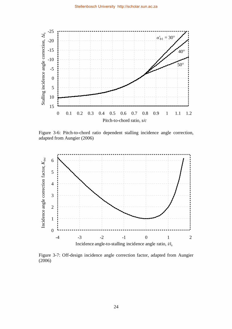
Figure 3-6: Pitch-to-chord ratio dependent stalling incidence angle correction,

adapted from Aungier (2006) ................................................................................ 24

Figure 3-7: Off-design incidence angle correction factor, adapted from Aungier

(2006) ..................................................................................................................... 24

Figure 3-8: Reynolds number correction factor, adapted from Aungier (2006) .... 26

Figure 3-9: Turbine stage exit static pressure based gas state calculation procedure

............................................................................................................................... 29

Figure 3-10: BMT 120 KS turbine empirical performance map at Tt0 = 1119 K, pt0

= 308300 Pa ........................................................................................................... 34

Figure 4-1: Turbine stage configuration ................................................................ 36

Figure 4-2: Geometrical constrains and turbine axial position definition ............. 38

Figure 4-3: Mollier diagram of a turbine stage ...................................................... 44

Figure 4-4: Optimal pitch to chord ratio for different combinations of blade inlet

and exit angles ....................................................................................................... 46

Figure 4-5: Quadratic Bézier curve camber line .................................................... 48

Figure 4-6: Variation of cubic Bézier curve camber line shapes ........................... 49

Figure 4-7: Blade thickness profile curve .............................................................. 50

Figure 4-8: New turbine design empirical performance analysis results ............... 51

Figure 4-9: Rotor blade profile stacking ................................................................ 53

Figure 5-1: Computational domain for a turbine simulation ................................. 55


xi

Figure 5-2: CFD boundary conditions ................................................................... 56

Figure 5-3: Computational mesh of the stator and inlet domains .......................... 57

Figure 5-4: BMT 102 KS turbine .......................................................................... 59

Figure 5-5: 95 % work coefficient design ............................................................. 60

Figure 5-6: 100 % work coefficient design ........................................................... 61

Figure 5-7: 105 % work coefficient design ........................................................... 61

Figure 6-1: FEM model structural constraints ....................................................... 64

Figure 6-2: Computational mesh of the 95 % work coefficient turbine design

model ..................................................................................................................... 66

Figure 6-3: Campbell diagram of the BMT 120 KS turbine rotor ......................... 68

Figure 6-4: Campbell diagram of the 95 % work coefficient turbine rotor ........... 69

Figure 6-5: Campbell diagram of the 100 % work coefficient turbine rotor ......... 69

Figure 6-6: Campbell diagram of the 105 % work coefficient turbine rotor ......... 70

Figure 7-1: Stator final (left) and casting (right) geometries ................................. 72

Figure 7-2: PrimeCast 101 rotor pattern ................................................................ 73

Figure 7-3: Solidscape 3Z Model rotor pattern ..................................................... 74

Figure 7-4: Ceramic mould destroyed by firing PrimeCast 101 stator patterns .... 75

Figure 7-5: Rotor casting made using a PrimeCast 101 pattern ............................ 76

Figure 7-6: Rotor casting made using a Solidscape 3Z Model pattern .................. 76

Figure 7-7: Stator casting made using a Solidscape 3Z Model pattern ................. 77


xii

List of tables

Table 3-1: Empirical performance model inlet parameters ................................... 18

Table 4-1: Geometrical design parameter selections ............................................. 39

Table 4-2: Current engine experimental test data at 120 krpm. ............................. 39

Table 4-3: Turbine inlet gas properties .................................................................. 40

Table 4-4: Turbine performance requirements ...................................................... 41

Table 5-1: CFD performance analysis inlet and outlet conditions ........................ 59

Table 6-1: Static structural analysis results ........................................................... 66

Table A-1: BMT 120 KS turbine stator blade row empirical performance model

inlet parameters ...................................................................................................... 81

Table A-2: Known parameter values at the stator inlet ......................................... 87

Table A-3: Known parameter values at the stator ex ............................................. 87

Table A-4: Known parameter values at the rotor inlet .......................................... 88

Table A-5: Known parameter values at the rotor exit ........................................... 90

Table B-1: Calculated turbine stage gas velocities ................................................ 95

Table B-2: Calculated turbine stage gas Mach numbers ....................................... 99

Table C-1: Domain length independence study results ....................................... 102

Table C-2: Mesh independence study results ...................................................... 103

Table D-1: Mechanical properties of Inconel IN713 LC ..................................... 104

Table D-2: Static structural mesh independence study results ............................ 105

Table D-3: Modal analysis mesh independence study results ............................. 105


xiii

Nomenclature

Roman symbols

Symbol Meaning

𝐴 Area

𝑎 Gas sonic velocity

𝑏𝑧 Axial chord

𝐶 Absolute gas velocity

𝐶𝐿 Lift coefficient

𝒄 Vector representing the starting point of a line in parametric space

𝑐 Point on a straight line at the zero parameter value, blade chord

𝑑 Diameter

𝑬 Vector representing the squared error of the three linear approximations

in parametric space

𝐸 Squared error of a linear approximation in parametric space

𝑒 Roughness height, calculation error

𝐹𝐴𝑅 Aspect ratio correction factor, area ratio correction

𝑓0 Static pressure ratio across the stator blade row

𝑓1 Static pressure ratio across the rotor blade row

𝐻 Blade height

ℎ Gas specific enthalpy

𝐼 Moment of inertia of a fluid particle

𝑖 Index running from 1 to k or from 0 to 3, incidence angle

𝑖𝑠 Stalling incidence angle

𝑖𝑠𝑟 ξ-Dependent term of the stalling incidence angle

∆𝑖𝑠 (s/c)-Dependent stalling incidence angle correction


xiv

𝑗 Index running from 1 to n

𝐾1 Factor used in calculating the compressibility correction factor, factor

used in calculating the turbine efficiency estimate

𝐾2 Standard tip clearance approximation

𝐾𝑖𝑛𝑐 Off-design Incidence angle correction factor

𝐾𝑀 Mach number correction factor for the profile loss coefficient

𝐾𝑚𝑜𝑑 Modern blade design modification factor for the profile loss coefficient

𝐾𝑝 Compressibility correction factor

𝐾𝑅𝐸 Reynolds number correction factor

𝐾𝑠 Modified form of the compressibility correction factor

𝑘 Number of sampled points on a given blade profile

𝐿 Angular momentum

𝑙 Camber line length

𝑙𝑡𝑜𝑡 Total camber line length

𝑀 Gas flow Mach number

𝑀′ Relative gas flow Mach number

�̃�′ Modified relative mach number

𝒎 Vector representing the slope of a line in parametric space

𝑚 Slope of the straight line

�̇� Mass flow rate

𝑁 Rotational speed, revolutions per minute

𝑛 Number of blade profiles

𝑃 Power output

𝒑 Vertex in three-dimensional space

𝑝 Pressure


xv

𝑅 Reaction ratio

𝑅𝑎𝑖𝑟 Gas constant for dry air, 278 J/kg/K

𝑅𝑐 Uncovered turning radius

𝑟 Radius

𝑠 Blade pitch

𝑠𝑜 Gas specific temperature dependend entropy

𝑇 Temperature

𝑡 Blade profile thickness

𝑈 Blade velocity

𝑊 Relative gas velocity

𝑋 Reaction ratio dependent aspect ratio correction

𝑋1 Shock loss contribution parameter

𝑋2 Diffusion loss contribution parameter

𝑋𝑖𝑠 (s/c)-Dependent parameters used to calculate ∆𝑖𝑠

𝑋𝑝 Factor used in calculating the compressibility correction factor

𝑥 Cartesian coordinate running along the blade length

𝑌 Relative total pressure loss coefficient, or component thereof

𝑌𝐶𝐿 Blade tip clearance loss coefficient

𝑌𝑝 Profile loss coefficient

𝑌𝑝1 Pure nozzle blade profile loss coefficient

𝑌𝑝2 Impulse blade profile loss coefficient

𝑌𝑠 Secondary flow loss coefficient

�̃�𝑠 Preliminary secondary flow loss coefficient

𝑌𝑆 Stator blade row relative total pressure loss coefficient


xvi

Greek symbols

𝑌𝑆𝐻 Shock loss coefficient

�̃�𝑆𝐻 Preliminary shock loss coefficient estimate

∆𝑌𝑇𝐸 Trailing edge loss correction factor

𝑦 Cartesian coordinate running tangent to the circumferential direction

𝑍 Ainley loading parameter

𝑧 Cartesian and polar coordate running in the axial direction, axial length

∆𝑧 Axial gap between stator and rotor

Symbol Meaning

𝛼 Gas flow angle

𝛼′ Relative flow angle

𝛼𝑚′ Mean relative flow angle

𝛽 Blade angle

𝛽𝑔 Blade gauge angle

𝛾 Stagger angle

𝛿 Tip clearance or deviation angle

𝛿0 Zero relative exit Mach number deviation angle

𝜂𝑡𝑡 Turbine total-to-total efficiency

𝜇 Gas dynamic viscosity

𝜉 Gas deflection ratio

𝜙 Stage flow coefficient

𝜓 Stage work coefficient

𝜔 Angular velocity

𝜉 Gas deflection ratio


xvii

Subscripts

Acronyms

Symbol Meaning

𝑏 Generic blade angle convention

𝐶 Compressor

ℎ Hub

𝑖𝑛 Inlet property

𝑚 Mean, or at mean radius

𝑚𝑎𝑥 Maximum

𝑜𝑝𝑡 Optimal

𝑜𝑢𝑡 Outlet

𝑠 Shroud

𝑇 Turbine

𝑡 Total conditions

𝑥 Cartesian coordinate along the blade length

𝑦 Cartesian coordinate tangent to the circumferential direction

𝑧 Cartesian and polar coordinate in the axial direction

𝜃 Circumferential direction

0, 1, 2, 3 Indices denoting positions throughout a turbine stage

ATM – Automatic Topology and Meshing

BMT – Baird Micro Turbine

CFD – Computational Fluid Dynamics

CMM – Coordinate Measuring Machine

CSIR – Council for Scientific and Industrial Research


xviii

CT – Computed Tomography

EM – Empirical Model

FEM – Finite Element Method

FINE – Flow Integrated Environment

KS – Kero Start

LE – Leading Edge

NURBS – Non-Uniform Rational B-Spline

PS – Pressure Surface

SAAF – South African Air Force

SS – Suction Surface

STL – Stereo Lithography

TE – Trailing Edge


1

1. Introduction

The Ballast project is a collaboration between the Counsil for Scientific and

Industrial Research (CSIR), the South African Air Force (SAAF), the Armaments

Corporation of South Africa (ARMSCOR) and the various universities within

South Africa. This project, funded by the SAAF, involves the training of

postgraduate students in the field of aerospace propulsion. Since its inception in

2010, the Ballast project has funded various research projects relating to the

design and analysis of micro gas turbine engines. The present project focuses on

the turbine stage of a micro jet engine. This thesis documents the research done

into compiling a methodology for designing axial-flow turbines for micro jet

engines.

1.1. Background and motivation

The Department of Mechanical and Mechatronic Engineering at Stellenbosch

University has been performing ongoing research in the field of small and micro

gas turbine engines. Recent years have seen a number of postgraduate students

completing projects in the design and analysis of jet engine components. The bulk

of the research has revolved around improving the performance of small

centrifugal compressors that are often used in micro gas turbine engines.

De Wet (2011) developed a method for analysing the performance of a diesel

locomotive turbocharger compressor using one-dimensional theory based on the

work of Aungier (2000). The results generated by this one-dimensional analysis

method were compared to centrifugal compressor test cases found in literature.

The comparison served to verify the accuracy of this one-dimensional method as a

centrifugal compressor analysis tool.

Van der Merwe (2012) used the one-dimensional centrifugal compressor

performance analysis program, developed by De Wet (2011), to design an

impeller for a micro gas turbine compressor. This design was then optimised for

certain pressure ratio, efficiency and mass flow rate targets using computational

fluid dynamics (CFD). Finite element methods (FEM) were used to analyse the

structure of this optimised compressor impeller design. The new impeller design

was finally manufactured and tested using the turbocharger test bench developed

as a postgraduate research project by Struwig (2012).

Krige (2012) focussed on the analysis and design of the radial diffuser for the

centrifugal compressor of a micro jet engine. The performance of the radial

diffuser in the Baird Micro Turbine 120 Kero Start (BMT 120 KS) micro turbojet

engine was evaluated using CompAero, a commercial one-dimensional analysis


2

program based on the centrifugal compressor theory by Aungier (2000). The

performance of the diffuser was also analysed using FINE Turbo, a commercial

CFD package developed by Numeca International. A replacement radial diffuser

for the BMT 120 KS compressor was designed and manufactured. The existing jet

engine, fitted with the new radial diffuser, was also tested experimentally using a

jet engine test bench that was constructed as part of the project.

The present project moves away from the study and development of centrifugal

compressors and focuses on the analysis and development of axial-flow turbines

found in micro jet engines. The goal of this project is the formulation of a

methodology for designing axial-flow turbines for use in small jet engines. Such a

design methodology must be able to generate a turbine design that conforms to the

dimensional restrictions and performance requirements that prevail in a micro jet

engine.

1.2. Objectives

The primary purpose of this study is to formulate a methodology for designing

axial-flow gas turbines for use in small jet engines. This is achieved through five

secondary objectives.

The first objective is to obtain a baseline turbine design to which any new design

can be compared. This design would have to be available in the different formats

required for different types of analyses.

The second objective is to develop a method for generating a viable candidate

(theoretical) turbine design for a given set of operational requirements. The

method should then be used to design a replacement turbine for the baseline

design obtained in meeting the first objective.

The third objective is to develop independent turbine performance analysis

procedures that investigate the suitability of a given turbine design for certain

operating conditions. Furthermore, a comparison of the results yielded by the

different analyses procedures would serve to validate the procedures themselves.

The fourth objective is to investigate the structural integrity of any candidate

design. Both the static and dynamic structural behaviour should be analysed to

ensure the viability of a given turbine design.

The fifth objective is to prove the manufacturability of new candidate design. A

manufacturing process, capable of producing prototypes of new turbine designs,


3

should be proposed. This process must then be implemented to create prototypes

of the new turbine designs.

1.3. Overview of the thesis

The presentation of the proposed design methodology is organised into six

sections. These sections form Section 2 to Section 7 of this thesis.

The start of the design process is described in Section 2, where a reverse

engineering process is used to generate a three-dimensional model of a turbine

from an existing engine. The geometries of the turbine stator and rotor are

digitised using respectively an X-ray computed tomography (CT) scanner and a

coordinate measuring machine (CMM). The raw data from the measurement

devices is then processed and reconstructed to yield three-dimensional models of

the two components. These models will form the baseline turbine design to which

any new designs could be compared.

In Section 3 a turbine performance analysis procedure that relies on an empirical

loss model is introduced. The empirical loss model is used to estimate the relative

total pressure loss coefficient of a blade row for given operating conditions. These

estimated loss coefficients for the stator and rotor blade rows are used in through

flow analyses to obtain the mass flow rates and the total-to-total efficiencies of a

turbine design for a range of pressure ratios. Since the computational cost of

obtaining the resulting turbine performance curves is low, this process is well

suited to an iterative design process.

A process for designing a single stage axial-flow turbine for an existing jet engine

is described in Section 4. This process involves determining the various

performance parameters and using these parameters to generate a turbine design

that would meet the requirements of the existing engine. The new turbine designs

can then be subjected to the performance analysis procedure described in Section

3. Such a performance assessment would then suggest whether further

investigation into each design is justified.

CFD performance analyses of the existing turbine and three new turbine designs

are shown in Section 5. The CFD methodology is detailed and the performance

analysis procedure is described. The results of the CFD performance analysis

would serve two purposes. Firstly the CFD results for a turbine design provide a

more accurate indication of the viability of that particular design. If the results of

a CFD analysis were to suggest that a turbine design would not perform

adequately, the analysis of such a design would not be pursued further. Secondly,


4

the CFD results of a turbine design can be compared to the corresponding results

of the performance analysis described in Section 3. Such a comparison could lead

to valuable insights into the validity of the two performance analysis tools.

In Section 6 the static structural and modal analyses of the existing turbine rotor

and the rotors of the three new designs are described. The FEM modelling is

detailed and the analysis methods are described. The static structural analysis

allows the structural integrity of the different turbine designs to be examined at

the operating conditions. The modal analysis enables the natural frequencies of

each turbine blade design to be compared to the excitation frequencies present at

any given rotational speed. Such a comparison is necessary for avoiding structural

resonance.

Section 7 documents the process followed to create the prototypes of the turbine

components. Firstly, the appropriate material for the prototypes is chosen, thus

enabling appropriate manufacturing processes to be specified. Three-dimensional

models of the desired final geometries are then generated and adapted as

necessitated by the chosen manufacturing processes. Finally, the results of the

different manufacturing processes can be compared.

Section 8 contains an overview of the results found in the preceding sections and

some concluding remarks.

1.4. A note on turbine blade and flow angle conventions

An angle convention is required when describing the flow field and blade

geometry of a turbo-machine. However, there is little standardization of flow

angle conventions in literature. Some authors use a plane through the axis of the

machine as the reference from where flow and blade angles are measured and

others measure the angles from the circumferential direction. Furthermore,

different authors differ in how the sign of a given angle is defined.

For the present design process an angle convention is defined that is consistent for

blade and flow field angles. All angles are measured from the axial direction and

are defined as positive in the direction of machine rotation. Figure 1-1 shows this

angle convention as applied to both the absolute and relative flow field angles, 𝛼

and 𝛼′ respectively, and the blade angles, 𝛽, for a single stage axial-flow turbine.

Negative angles are shown by dotted line arrows.


5

Figure 1-1: Consistent blade and flow angle convention

Despite the author’s attempt to use only one angle convention, a generic blade

angle convention is also used due to its compatibility with certain published

empirical correlations. In this generic blade convention angles are measured from

the circumferential direction and always from the pressure, or concave, side of the

blade. This convention is shown in Figure 1-2 as it is applied to the same axial-

flow turbine stage shown in Figure 1-1. As shown in Figure 1-2 all the angles are

defined positive, so one can’t deduce whether a blade is a rotor or a stator blade

by observing the angle signs.

Figure 1-2: Generic blade angle convention

𝛼0

𝛼1 𝛼′2

𝛼′3

𝛽0

𝛽1

𝛽2

𝛽3

Stator blade

Rotor blade

𝛼𝑏0

𝛽𝑏0

𝛼𝑏1

𝛽𝑏1

𝛼′𝑏2

𝛽𝑏2

𝛼′𝑏3

𝛽𝑏3

Stator blade

Rotor blade


6

The translation between the consistent convention and the generic blade angle

conventions for a turbine stage is shown is equations (1.1) through (1.4). This

translation is shown only for the blade angles, but it also applies to the absolute

and relative flow field angles.

𝛽𝑏0 = 90° + 𝛽0 (1.1)

𝛽𝑏1 = 90° − 𝛽1 (1.2)

𝛽𝑏2 = 90° − 𝛽2 (1.3)

𝛽𝑏3 = 90° + 𝛽3 (1.4)

(Cohen, et al., 1996)

(Japikse & Baines, 1994)

(Creci, et al., 2010)

(Krige, 2012)

(Nickel Development Institute, 1995)

(Ainley & Mathieson, 1951)

(Aungier, 2006)

(Struwig, 2012) (De Wet, 2011) (Van der Merwe, 2012)


7

2. Reverse engineering an existing turbine

2.1. Introduction

This section describes how the geometries of the stator and the rotor wheels of the

BMT 120 KS engine are digitized as part of a process known as reverse

engineering. Reverse engineering allows structural and performance analyses to

be performed on the components of an existing turbine stage. The results of these

analyses are then used as a baseline to which the performance of any new turbine

stage design is compared. Reverse engineering is widely recognised as an

essential step in the design cycle (Chen & Lin, 2000).

The rotor wheel has two complex geometrical features that require high resolution

sampling: the axisymmetric hub profile and the radially varying blade profile.

These two features are digitized by using a three-dimensional coordinate

measuring machine (CMM) to record traces of points along the aforementioned

profiles.

The stator wheel also has complex blade profiles, but the hub and shroud profiles

are simple cylindrical surfaces that can be defined by a small number of easily

measured variables. Therefore only the blades of the stator wheel need to be

sampled at a high resolution. An X-ray computed tomography (CT) scanner is

used to create a point cloud of the stator wheel, since the shroud restricts the

physical access to the blades for profile measuring.

The digitisations of the turbine components as they are collected from the

measurement instruments are in a point cloud format. These point clouds are

processed to yield usable geometries of the physical features they represent.

Finally the processed geometric information is compiled into complete three-

dimensional models of the turbine components.

2.2. Component point cloud extraction

2.2.1. Obtaining turbine rotor point cloud data using a CMM

A Mitutoyo Bright STRATO 710 coordinate measuring machine (CMM), shown in

Figure 2-1, is used to generate the turbine rotor point cloud. CMMs have the

ability to measure the coordinates of points on the surface of an object very

accurately and are well suited to measuring the complex shapes found in turbine

blades (Junhui, et al., 2010). The present CMM has a precision ground granite

table to serve as a flat reference surface to which the measured object is secured.

The granite table top also has various mounting holes that accept auxiliary


8

precision machined mounting blocks. These blocks provide additional

configuration options when mounting an object.

Figure 2-1: Mitutoyo Bright Apex 710

The measurements are made using a contact sensitive computer numerically

controlled (CNC) probe. The end of the probe is equipped with a stylus consisting

of a metal stem with a spherical ball at its tip. The probe is moved in the vicinity

of the object and the coordinates of the end-ball are recorded whenever contact

with the object is made.

The radius of the end-ball imposes a constraint on the minimum radius of

curvature that can be perceived by the CMM. Clearly the CMM cannot detect a

concave curve that has a radius of less than the radius of the probe end-ball.

However, using a larger ball increases the reach of the probe when measuring

surfaces under overhanging features like curved turbine blades.

The machine set-up and part configuration

The turbine rotor wheel is temporarily glued to a mounting block that is in turn

attached to the CMM table. This use of a mounting block allows the turbine rotor

to be secured with its rotational axis parallel to the table and one of the blades

pointing directly upward. The configuration of the turbine rotor is shown in

Figure 2-2 where the illustrations of the turbine rotor wheel, the mounting block


9

and the granite table of the CMM can be seen. This configuration permits the

CMM probe to record the coordinates of a large number of points along the blade

profile at a fixed height above the table. Additionally, this setup allows the probe

unobstructed access to one side of the hub of the turbine rotor wheel.

Figure 2-2: CMM turbine rotor configuration

The measurement paths

Rotor blade profile

The variation of the turbine rotor blade profile from its root to its tip is digitised

by recording point traces at different radial positions along the blade length. The

CMM probe is constrained to a height above the table slightly below the tip of the

upward facing turbine blade. The probe then follows a path along the blade

surface at that height and records the coordinates of the points where the end-ball

contacts the surface. This process is repeated a number of times with the fixed

height being moved downwards incrementally. The lowest possible fixed height is

slightly above the blade root since the hub of the turbine rotor would interfere

with the path of the probe. This process yields blade profile data that ranges from

slightly below the blade tip to slightly above the blade root.

Rotor hub profile

The rotor hub contour is digitised by recording a point trace starting in the centre

of the shaft hole and moving radially outwards. This is accomplished by keeping

the probe at a fixed height and allowing it to follow the hub profile until it reaches

the blade root.


10

Figure 2-3 shows the paths followed by the CMM probe as black lines. It can be

seen that the blade profile is sampled at six locations and the trace along the hub

profile is also visible.

Figure 2-3: CMM measurement paths on the turbine rotor wheel

2.2.2. Obtaining turbine stator wheel point cloud data from CT-scanner

data

X-ray computed tomography (CT) scanners can produce a three-dimensional

point cloud of an object by integrating information from different X-ray images of

the object. A high-resolution CT-scanner, the Phoenix v|tome|x m shown in Figure

2-4 on the next page, is used to create a three-dimensional point cloud of the

turbine stator wheel.

The CT-scanner software outputs the point cloud data in a stereo lithography

(STL) file format. This file is not a solid model, but rather a collection of point

coordinates. It is however possible to draw surfaces between all sufficiently close

neighbouring points in order to visualise the CT-scanner output. Such

visualisations of the front and back views of the stator wheel point cloud are

shown in Figure 2-5 on the next page. These visualisations can be used to assess

the quality of the geometric reproduction produced by the CT-scanner.


11

Figure 2-4: Phoenix v|tome|x m high resolution CT-scanner

Figure 2-5: Surface visualization of STL-file produced by the CT-scanner

Referring to Figure 2-5, it can be seen that the CT process results in a model with

feature reproduction in some areas. This geometrical distortion is most apparent

near the mounting holes of the stator wheel, but is also visible on most of the

blades.

Front view Back view


12

The software of a CT-scanner uses the physical properties of the object material in

translating the input signal from its X-ray detector into meaningful geometries.

Therefore a possible reason for the lack in model quality is the presence of foreign

material deposits on the turbine stator wheel during the scanning process. Such

deposits are likely to have accumulated, due the present stator wheel operating in

a working micro gas turbine engine. During high temperature operation both the

locking compound used on the mounting holes and the incomplete combustion

process close to the blades leave a residue. For the present case the areas affected

by geometric distortion coincide with the areas where contaminant residue is

found. Therefore the presence of the residue is deemed a plausible explanation for

the geometric distortion.

Fortunately one of the stator blades is unaffected by the geometrical distortion

along most of its span. This undistorted blade enables the extraction of the stator

blade profile data from the CT-scanner generated point-cloud. Furthermore, the

badly distorted mounting hole geometry is not critical to the performance analysis

of the turbine. Therefore the CT-scanner produced usable data for the reverse

engineering process.

2.3. Processing raw point coordinate data

2.3.1. Curve smoothing

The CMM yields the coordinates of discrete points on the surfaces of the turbine

rotor blade wheel hub. Due to the small size of these features and the roughness of

these surfaces the resulting collections of points contain a certain amount of noise.

Therefore, non-uniform rational B-spline (NURBS) curves are fitted through each

collection of points in order to obtain smooth profile curves for both the rotor

blades and rotor wheel hub. These NURBS curves provide a curve that is an

appropriate average of the measured points.

Similarly, the point cloud model of the stator wheel generated by the CT-scanner

is also geometrically noisy. Parametric surfaces are therefore fitted through the

points in the vicinity of the surface of the least distorted blade portion. These

surfaces are constrained to be continuous in curvature and wrap all the way

around the central part of the blade span. Slices are then made through the

surfaces to obtain smooth blade profile curves.

2.3.2. Blade profile extrapolation

During measurement operations, it is not possible to obtain accurate

measurements of points on the edges of an object (Chivate & Jablokow, 1995).

Therefore, for both the turbine rotor and the stator, smoothed blade profile curves


13

only cover the central portion of the blade span. However, the complete three-

dimensional reconstructions of the blades require blade profiles that include the

root and tip sections. Since these additional profile curves could not be measured,

linear extrapolations of the blade profiles are performed.

The blade profile curves are each divided into four curve sections according to

local radius of curvature. These sections relate to the blade leading edge (LE),

trailing edge (TE), pressure surface (PS) and suction surface (SS) respectively.

Dividing the turbine profile into these functional regions strongly improves the

accuracy with which the geometry can be recreated (Mohaghegh, et al., 2006).

Figure 2-6 shows one such blade section division where the four different sections

are identified. The leading and trailing edge curves can be seen to have small

curvature radii compared to those of the pressure and suction surface curves.

Figure 2-6: Blade profile curve section divisions

The leading edge curve section of each blade profile curve is sampled at a fixed

number of evenly distributed points as shown in Figure 2-7. This is done to relate

each point on the leading edge curve of one blade profile curve to a corresponding

point on the leading edge curve of every other profile curve. This process is

repeated for the remaining three curve sections of each blade profile curve to yield

a set of consistently sampled profile curves.

LESS

PS

TEx

y

z


14

Figure 2-7: LE curve section point sampling

Given that the each of the 𝑛 profile curves has 𝑘 consistently sampled points, the

point data can now be represented as point 𝑖 on profile 𝑗, or symbolically as

𝒑𝑖,𝑗 = {

𝑥𝑖

𝑦𝑖

𝑧𝑖

}

𝑗

, 𝑖 ∈ [1, 𝑘], 𝑗 ∈ [1, 𝑛]. (2.1)

A linear regression can now be done for each set of 𝑛 corresponding points on the

different blade profile curves. The linear trend line is calculated using the least

squares criterion and using the radius about the turbine rotational axis as the

independent variable. The radius of each point is given by

𝑟𝑖,𝑗 = √𝑥𝑖,𝑗2 + 𝑦𝑖,𝑗

2 . (2.2)

The three-dimensional line is represented by three parametric equations: one for

the x-direction, one for the y-direction, and one for the z-direction. These

parametric equations are of the form:

𝒑𝒊(𝑟) = 𝒎𝒊𝑟 + 𝒄𝒊, 𝒎𝒊 = {

𝑚𝑥

𝑚𝑦

𝑚𝑧

}

𝒊

, 𝒄𝒊 = {

𝑐𝑥

𝑐𝑦

𝑐𝑧

}

𝑖

. (2.3)

The total squared error of each linear approximation, 𝑬𝑖, is

𝑬𝑖 = {

𝐸𝑥

𝐸𝑦

𝐸𝑧

}

𝑖

= ∑

{

[(𝑚𝑥,𝑖𝑟𝑖,𝑗 + 𝑐𝑥,𝑖) − 𝑥𝑖,𝑗]

𝟐

[(𝑚𝑦,𝑖𝑟𝑖,𝑗 + 𝑐𝑦,𝑖) − 𝑦𝑖,𝑗]𝟐

[(𝑚𝑧,𝑖𝑟𝑖,𝑗 + 𝑐𝑧,𝑖) − 𝑧𝑖,𝑗]𝟐

}

𝑛

𝑗=1

. (2.4)

The values of the parametric equation coefficients, 𝒎𝒊 and 𝒄𝑖, are found by first

partially differentiating the error function with respect to each coefficient. The

procedure is only shown for the 𝑥-component of the parametric equation, but the

formulation is identical for the 𝑦-component and 𝑧-component.

LE curve

LE

sampling points

x

y

z


15

𝜕𝐸𝑥,𝑖

𝜕𝑚𝑥,𝑖= ∑(2𝑚𝑥,𝑖𝑟𝑖,𝑗

2 + 2𝑐𝑥,𝑖𝑟𝑖,𝑗 − 2𝑥𝑖,𝑗𝑟𝑖,𝑗)

𝑛

𝑗=1

(2.5)

𝜕𝐸𝑥,𝑖

𝜕𝑚𝑥,𝑖= ∑(2𝑚𝑥,𝑖𝑟𝑖,𝑗 + 2𝑐𝑥,𝑖 − 2𝑥𝑖,𝑗)

𝑛

𝑗=1

(2.6)

These derivatives are then equated to zero, thus resulting in a system of linear

equations. The system is written in matrix form and solved by inversion:

[∑𝑟𝑖,𝑗

2 ∑𝑟𝑖,𝑗∑𝑟𝑖,𝑗 𝑛

] {𝑚𝑥,𝑖

𝑐𝑥,𝑖} = {

∑𝑟𝑖,𝑗𝑥𝑖,𝑗

∑𝑥𝑖,𝑗} (2.7)

{𝑚𝑥,𝑖

𝑐𝑥,𝑖} = [

∑𝑟𝑖,𝑗2 ∑𝑟𝑖,𝑗

∑𝑟𝑖,𝑗 𝑛]

−1

{∑𝑟𝑖,𝑗𝑥𝑖,𝑗

∑𝑥𝑖,𝑗} (2.8)

Therefore there exist three linear systems for each of the 𝑘 consistently sampled

profile points. Once all the systems are solved the blade can be defined as a

function of radius, using the resulting parametric equations. These equations are

then used to generate blade profile points that range from the blade root to the

blade tip.

2.4. Three-dimensional model reconstruction

Once the blade profiles are available for the whole length of the blades, these

profiles are imported into a CAD package. In the CAD package a surface loft is

performed on the profiles, yielding the blade surfaces. These blade surfaces

provide sufficient geometrical data to perform CFD and empirical model based

performance analyses.

The aim is however to generate full three-dimensional models of the two turbine

components. To achieve this, the hubs of the turbine rotor and the stator, and the

shroud of the latter must be modelled. The hub profile of the rotor wheel is

available, since it was digitised along with its blade profiles. The hub and shroud

profiles of the stator wheel are much simpler geometries and easily obtained using

a vernier calliper. These profiles are then revolved around the turbine axis of

rotation to obtain solid models of the rotor hub and the stator hub and shroud.

Finally, the blade surfaces are mated to their respective hub and shroud surfaces to

complete the three-dimensional component models. Fillet radii are applied where

the blades meet the hub or shroud surfaces and the blades are patterned circularly

around the axis of the turbine for the correct number of blades. Figure 2-8 shows


16

the resulting three-dimensional models of the turbine stator (left) and the rotor

(right).

Figure 2-8: Three-dimensional turbine stator and rotor wheel reconstructions

2.5. Conclusion

This section presented the process followed in reverse engineering the turbine

components found in the BMT 120 KS micro jet engine. The turbine rotor was

digitised using a CMM and the turbine stator was digitised using a CT-scanner.

The raw point cloud data generated by the two measurement devices was

processes to allow for the reconstruction of full three-dimensional models of the

two turbine components.


17

3. Performance analysis using an empirical loss model

3.1. Introduction

Turbine performance analyses are required during the design process to ensure the

viability of any given combination of design parameters. Clearly, the most

accurate method for analysing a turbine design is to build a prototype and perform

a full experimental test. Such a method is essential in the final design stage, but its

high cost and long lead times make it impractical during the early design stage.

An alternative performance analysis method that can yield highly accurate results

is a full three-dimensional computational fluid dynamics (CFD) analysis. These

analyses are less expensive and less time consuming than experimental testing.

However, the set-up and run time of such an analysis is too long for the rapid

evaluation of many different designs. Therefore a low-cost and less time

consuming analysis method is required. An empirical loss model can be

incorporated into a one-dimensional mean-radius performance analysis system

that is both low-cost and has a negligible run time.

In a one-dimensional mean-radius performance analysis system the gas states and

velocities are calculated throughout the turbine stage using isentropic

thermodynamic relationships. The entropy generation losses in the turbine stage

are then accounted for by means of empirical correlations.

3.2. Empirical loss model

The use of an empirical loss model is an attempt to assess the performance of a

turbine blade row without actually testing or simulating it. In the absence of actual

test data for a given design, the effects of different design parameters on the

performance of previously tested turbine designs are correlated. These empirical

correlations are then used to estimate the effects of each design parameter on the

untested design.

In an adiabatic blade row, the entropy generation is linearly dependent on the total

pressure loss through the blade row (De la Calzada, 2011). Therefore, the

empirical loss model proposed by Ainley and Matthieson (1951) predicts the

effect different design parameters have on the total pressure loss across a given

blade row. This loss in total pressure is accounted for by a total pressure loss

coefficient. The total pressure loss coefficient of a blade row, 𝑌, is defined as the

ratio of the loss of relative total pressure across the blade row to the dynamic

pressure at the exit of the blade row. This definition is shown symbolically in

equation (3.1).


18

𝑌 =𝑝𝑡0

′ − 𝑝𝑡1′

𝑝𝑡1′ − 𝑝1

(3.1)

The present loss model calculates the value of 𝑌 by estimating and summing the

effects of five different sources of irreversibility present in the blade row. These

sources are the blade profile loss (𝑌𝑝), secondary flow loss (𝑌𝑠), tip clearance loss

(𝑌𝐶𝐿), the non-zero blade trailing edge thickness loss (𝑌𝑇𝐸), and the loss caused by

the formation of shock waves (𝑌𝑆𝐻). Therefore the present total pressure loss

model can be expressed as:

𝑌 = 𝑌𝑇𝐸 + 𝑌𝑝 + 𝑌𝑠 + 𝑌𝐶𝐿 + 𝑌𝑆𝐻 . (3.2)

3.2.1. Loss model parameters

The loss model predicts the performance by estimating the contribution of

different design parameters to the overall total pressure loss of a blade row. These

parameters are listed in Table 3-1.

Table 3-1: Empirical performance model inlet parameters

The blade height, tip clearance and surface roughness height all have

unambiguous meanings, and so do the relative Mach numbers and thermodynamic

properties of the flow field. The rest of the parameters are defined in Figure 3-1

where the profiles of two neighbouring blades are shown. As can be seen in

Figure 3-1, the blade gauge angle is the angle measured from the tangent to the

suction side of the blade between its trailing edge and the throat to the

circumferential direction. This angle can fairly easily be measured by hand using

an appropriately sized mitre gauge.

Blade parameters Flow field parameters

𝛽𝑏0 Inlet blade angle 𝛼𝑏0′ Relative inlet angle

𝛽𝑔 Gauge angle 𝛼𝑏1′ Relative exit angle

𝑏𝑧 Axial chord 𝑊1 Relative exit velocity

𝑐 Chord 𝑀0′ Relative inlet Mach number

𝑠 Mean radius blade pitch 𝑀1′ Relative exit Mach number

𝑠/𝑐 Pitch-to-chord ratio 𝜌1 Exit density

𝑅𝑐 Uncovered turning radius 𝜇1 Exit dynamic viscosity

𝑡𝑚𝑎𝑥 Maximum thickness

𝑡𝑇𝐸 Trailing edge thickness

𝑒 Surface roughness height

𝐻 Height

𝛿 Tip clearance


19

Figure 3-1: Blade and flow field parameters

3.2.2. Trailing edge loss coefficient

The finite trailing edge thicknesses of turbine blades cause the flow to separate

from the blade at two separate points: one on each side of the blade. The present

model proposed by Aungier (2006) treats the effects of this flow separation as a

sudden flow area enlargement, resulting in the expression for the trailing edge loss

coefficient shown in equation (3.3).

𝑌𝑇𝐸 = (𝑡𝑇𝐸

𝑠 sin𝛽𝑔 − 𝑡𝑇𝐸)

2

(3.3)

3.2.3. Profile loss coefficient

The profile loss coefficient is influenced by a number of different factors and

defined by Equation (4-21) on page 69 in Aungier (2006),

𝑌𝑝 = 𝐾𝑚𝑜𝑑 𝐾𝑖𝑛𝑐 𝐾𝑀 𝐾𝑝 𝐾𝑅𝐸 ((𝑌𝑝1 + 𝜉2(𝑌𝑝2 − 𝑌𝑝1)) (5 𝑡𝑚𝑎𝑥

𝑐)

𝜉

− 𝛥𝑌𝑇𝐸). (3.4)

𝛽𝑏1

𝛽𝑏0

𝑅𝑐

𝑏𝑧

𝑠

𝛽𝑔

𝑡𝑇𝐸

𝑡𝑚𝑎𝑥

𝑐

Camber line


20

This expression consists of a base profile loss coefficient, 𝑌𝑝1 + 𝜉2(𝑌𝑝2 − 𝑌𝑝1),

and a number of modification factors and terms. The different factors in the

profile loss coefficient expression are now identified and defined.

Nozzle blade and impulse blade profile loss coefficients, 𝒀𝒑𝟏 and 𝒀𝒑𝟐

The base profile loss coefficient of an airfoil is calculated by interpolating

between the coefficients for a pure nozzle blade and an impulse blade of the same

exit angle. The term “pure nozzle blade” used here refers to a blade with an inlet

angle of 𝛽0𝑏 = 90°. The gas deflection ratio, 𝜉, is used in the interpolation

calculation and defined as the ratio of the inlet blade angle to the exit flow angle:

𝜉 =90° − 𝛽𝑏0

90° − 𝛼𝑏1′ . (3.5)

Both the nozzle blade and the impulse blade profile loss coefficients are functions

of the relative outlet flow angle and the difference between the actual and

optimum pitch-to-chord ratios. The optimum pitch-to-chord ratios for nozzle

blades and impulse blades according to Aungier (2006) are shown in Figure 3-2

for a range of possible relative exit flow angles. The equations for calculating the

optimum nozzle blade and impulse blade pitch-to-chord ratios are shown in

Appendix A.1.2 as equations (A-5) and (A-6) respectively.

Figure 3-2: Optimum pitch-to-chord ratios for nozzle and impulse blades

according to Aungier’s (2006) correlation

0.3

0.4

0.5

0.6

0.7

0.8

0.9

1

1.1

1.2

5 10 15 20 25 30 35 40 45 50 55 60 65 70

Opti

mum

pit

ch-t

o-c

hord

rat

io, (s

/c) o

pt

Relative exit flow angle, α'b1, degrees

Nozzle blade

Impulse blade


21

The nozzle blade profile loss coefficient, 𝑌𝑝1, is a function of the exit blade angle

and the difference between the actual and the optimal nozzle blade pitch-to-chord

ratios. 𝑌𝑝1 is calculated using equations (A-7) to (A-12) in Appendix A.1.2.

Similarly, the impulse blade profile loss coefficient, 𝑌𝑝2, is a function of the exit

blade angle and the difference between the actual and the optimal impulse blade

pitch-to-chord ratios. 𝑌𝑝2 is calculated using equations (A-13) to (A-17) in

Appendix A.1.2. These nozzle blade and impulse blade profile loss coefficients

according to Aungier (2006) are shown in Figure 3-3 and Figure 3-4 respectively

for different pitch-to-chord ratios and different relative exit flow angles.

Figure 3-3: Profile loss coefficient for nozzle blades, adapted from Aungier

(2006)

Modification factor for modern blade designs

The modification factor for modern blade designs, 𝐾𝑚𝑜𝑑, is suggested by Kacker

and Okapuu (1982) to take the advances in modern blade design into account

when predicting the profile loss coefficient of a blade row. It assumes a reduction

in profile loss ranging from 33 % for highly optimized designs to 0 % for old non-

optimised designs. For the present case the blade design is not formally optimised.

Consequently it is treated as an older design and the modification factor assumes a

value of unity.

𝐾𝑚𝑜𝑑 = 1. (3.6)

0

0.01

0.02

0.03

0.04

0.05

0.06

0.07

0.08

0.09

0.1

0.1 0.2 0.3 0.4 0.5 0.6 0.7 0.8 0.9 1 1.1 1.2

Nozz

le b

lad

e pro

file

loss

coef

fici

ent,

Y

p1

Pitch-to-chord ratio, s/c

α'b1 = 10

15

20

30

50


22

Figure 3-4: Profile loss coefficient for impulse blades, adapted from Aungier

(2006)Off-design incidence correction factor

The off-design incidence correction factor, 𝐾𝑖𝑛𝑐, takes account of the difference

between the inlet blade angle and the relative inlet flow angle, or incidence angle,

during off-design operation. The incidence angle at any operating condition is

given by

𝑖 = 𝛽𝑏0 − 𝛼𝑏0′ . (3.7)

The amount of correction required depends on the ratio of the actual incidence

angle to the incidence angle that would induce blade stall. An empirical

correlation is employed to predict the stalling incidence angle. The stalling

incidence angle correlation is built up from a gas deflection ratio dependent

part, 𝑖𝑠𝑟, and a blade pitch-to-chord ratio dependent stalling incidence angle

correction, ∆𝑖𝑠.

𝑖𝑠 = 𝑖𝑠𝑟 + ∆𝑖𝑠 (3.8)

The gas deflection ratio dependent part of the stalling incidence angle is also a

function of the relative gas exit angle. The interrelationship between these three

variables as modelled by Aungier (2006) is shown in Figure 3-5. In Figure 3-5 the

gas deflection ratio dependent part of the stalling incidence angle is shown for six

different relative exit flow angles. The equations used to model the gas deflection

ratio dependent part of the stalling incidence angle are shown in Appendix A.1.2

as equations (A-19) to (A-24).

0.04

0.06

0.08

0.1

0.12

0.14

0.16

0.18

0.2

0.22

0.24

0.26

0.1 0.2 0.3 0.4 0.5 0.6 0.7 0.8 0.9 1 1.1

Impuls

e bla

de

pro

file

loss

coef

fici

ent,

Y

p2

Pitch-to-cord ratio, (s/c)

α'b1 = 10

15

20

30

50


23

Figure 3-5: Gas deflection ratio dependent stalling incidence angle term, adapted

from Aungier (2006)

The pitch-to-chord ratio dependent stalling incidence angle correction is

calculated using equations (3.9) and (3.10), and is shown in Figure 3-6 for three

different relative exit flow angles. (Aungier, 2006)

𝑋𝑖𝑠 = 𝑠/𝑐 − 0.75 (3.9)

∆𝑖𝑠 = {

−38°𝑋𝑖𝑠 − 53.5°𝑋𝑖𝑠2 − 29°𝑋𝑖𝑠

3 , 𝑠/𝑐 ≤ 0.8

−2.0374° − (𝑠/𝑐 − 0.8) [69.58° − 1° (𝛼𝑏1

′

14.48°)

3.1

] , 𝑠/𝑐 > 0.8 (3.10)

Finally, the off-design incidence correction factor is calculated using equation

(3.11)Error! Reference source not found. and is shown in Figure 3-7 for a range

of different actual-to-stalling incidence angle ratios.

𝐾𝑖𝑛𝑐 =

{

−1.39214 − 1.90738(𝑖/𝑖𝑠) , (𝑖/𝑖𝑠) < −3

1 + 0.52(𝑖/𝑖𝑠)1.7, −3 ≤ (𝑖/𝑖𝑠) < 0

1 + (𝑖/𝑖𝑠)2.3+0.5(𝑖/𝑖𝑠), 0 ≤ (𝑖/𝑖𝑠) < 1.7

6.23 − 9.8577[(𝑖/𝑖𝑠 ) − 1.7], 1.7 ≤ (𝑖/𝑖𝑠)

(3.11)

0

5

10

15

20

25

30

35

40

45

50

55

60

65

-1.2 -1.0 -0.8 -0.6 -0.4 -0.2 0.0 0.2 0.4 0.6 0.8 1.0 1.2 1.4

ξ-d

epen

den

t st

alling in

cid

ence

angle

, i s

r

Gas deflection ratio, ξ

α'b1 = 5

20

30

40

10

60


24

Figure 3-6: Pitch-to-chord ratio dependent stalling incidence angle correction,

adapted from Aungier (2006)

Figure 3-7: Off-design incidence angle correction factor, adapted from Aungier

(2006)

-25

-20

-15

-10

-5

0

5

10

15

0 0.1 0.2 0.3 0.4 0.5 0.6 0.7 0.8 0.9 1 1.1 1.2

Sta

llin

g inci

den

ce a

ngle

corr

ecti

on, Δ

i s

Pitch-to-chord ratio, s/c

α'b1 = 30

40

50

0

1

2

3

4

5

6

-4 -3 -2 -1 0 1 2

Inci

den

ce a

ngle

corr

ecti

on f

acto

r, K

inc

Incidence angle-to-stalling incidence angle ratio, i/is


25

Mach number correction factor

𝐾𝑀 is a correction factor that is dependent on the relative exit flow Mach number

of the blade row. It is based on the graphical data published by Ainley and

Mathieson (1951) and takes the form of an empirical correlation. The correlation,

proposed by Aungier (2006), closely approximates the graphical data and is

shown in symbolic form in equation (3.12).

𝐾𝑀 = 1 + [1.65(𝑀1′ − 0.6) + 240(𝑀1

′ − 0.6)4] (𝑠

𝑅𝑐)

3𝑀1′−0.6

(3.12)

Equation (3.12) is applicable when the relative exit flow Mach number is between

0.6 and 1. For Mach number values outside of this range 𝐾𝑀 assumes a value of

unity. For Mach numbers of 0.6 or less no correction factor is required; and for

Mach numbers of 1 or more the correction is made with a different factor.

Compressibility correction factor, 𝑲𝒑

Turbines experience higher Mach number flows during operation than can be

obtained in low speed cascade testing. The compressibility accompanying these

higher Mach numbers lead to thinner boundary layers and a decreased likelihood

of flow separation (Japikse & Baines, 1994). These two effects serve to decrease

the profile loss below the value predicted by a loss model based solely on cascade

testing. Therefore 𝐾𝑝 is included in this loss model to take account of these

benefits of the higher Mach number flow conditions present in actual turbine

operation.

Kacker and Okapuu (1982) originally suggested a correction factor based on the

relative inlet and outlet Mach numbers of a blade row. This formulation can

however result in negative profile loss coefficients for certain unlikely relative

inlet and outlet Mach number combinations. Therefore Aungier (2006) proposes a

revision of the Kacker and Okapuu formulation that limits 𝐾𝑝 to values greater

than about 0.5. The revised formulation used in the present loss model is

(Aungier, 2006):

�̃�0′ = 0.5(𝑀0

′ + 0.566 − |0.566 − 𝑀0′ |) (3.13)

�̃�1′ = 0.5(𝑀1

′ + 1 − |𝑀1′ − 1|) (3.14)

𝑋𝑝 =2�̃�0

′

�̃�0′ + �̃�1

′ + |�̃�1′ − �̃�0

′ | (3.15)

𝐾1 = 1 − 0.625(�̃�1′ − 0.2 + |�̃�1

′ − 0.2|) (3.16)

𝐾𝑝 = 1 − (1 − 𝐾1)𝑋𝑝2. (3.17)


26

Reynolds number correction factor, 𝑲𝑹𝑬

The data from which the loss model is deduced is obtained from cascade tests at a

certain flow Reynolds number. 𝐾𝑅𝐸 is used to adjust the profile loss coefficient for

the higher Reynolds numbers encountered in turbine operation. The correction

depends on the flow regime and is therefore treated differently for laminar,

transition and turbulent flows. The present model, proposed by Aungier (2006),

also takes blade surface roughness into account. Figure 3-8 shows how the 𝐾𝑅𝐸 of

this model varies with the chord based Reynolds number, 𝑅𝑒𝑐, for different values

of chord length-to-surface roughness height ratio, 𝑐/𝑒. The equations used to

model the Reynolds numbers correction factor are shown in Appendix A.1.2 as

equations (A-36) to (A-40).

Figure 3-8: Reynolds number correction factor, adapted from Aungier (2006)

Trailing edge loss correction factor, ∆𝒀𝑻𝑬

Ainley and Mathieson (1951) included a trailing edge loss in their model,

specifically assuming a trailing edge thickness of 2 % of a pitch, or 𝑠/50. This

present model accounts for the trailing edge loss separately, so therefore the loss

accounted for in the Ainley Mathieson model must be subtracted. ∆𝑌𝑇𝐸 assumes

the value calculated by the present trailing edge loss model for a trailing edge

thickness of 𝑠/50.

∆𝑌𝑇𝐸 = 𝑌𝑇𝐸(𝑡𝑇𝐸 = 0.02𝑠) (3.18)

0.0

0.2

0.4

0.6

0.8

1.0

1.2

1.4

1.6

1.8

2.0

1.E+4 1.E+5 1.E+6 1.E+7 1.E+8 1.E+9

Rey

no

lds

nu

mb

er c

orr

ecti

on

fac

tor,

K

RE

Chord-based Reynolds number, Rec

c/e = 1000

2000

5000

20000

200000


27

∆𝑌𝑇𝐸 = (0.02𝑠

𝑠 sin𝛽𝑔 − 0.02𝑠)

2

(3.19)

3.2.4. Secondary flow loss coefficient

The secondary flow loss coefficient, 𝑌𝑠, is modelled as a preliminary estimate, 𝑌�̃�,

adjusted to take account of the Reynolds number and compressibility effects:

𝑌𝑠 = 𝐾𝑅𝐸𝐾𝑠√�̃�𝑠

2

1 + 7.5�̃�𝑠2 . (3.20)

𝐾𝑅𝐸 is the Reynolds correction number shown in Figure 3-8 and 𝐾𝑠 is a modified

form of the compressibility correction factor expressed in equation (3.17). 𝐾𝑠 is

defined as

𝐾𝑠 = 1 − (1 − 𝐾𝑝) [(𝑏𝑧/𝐻)2

1 + (𝑏𝑧/𝐻)2] . (3.21)

The preliminary secondary flow loss coefficient is given by:

�̃�𝑠 = 0.0334𝐹𝐴𝑅𝑍sin𝛼𝑏1

′

sin 𝛽𝑏0, (3.22)

where 𝐹𝐴𝑅 is the aspect ratio correction factor and 𝑍 is the Ainley loading

parameter. These are respectively defined as

𝐹𝐴𝑅 = {0.5 (2𝑐

𝐻)

0.7

, 𝐻/𝑐 < 2

𝑐/𝐻, 𝐻/𝑐 ≥ 2

(3.23)

and

𝑍 = (𝐶𝐿

(𝑠/𝑐))

2 sin2 𝛼𝑏1′

sin3 𝛼𝑚′ . (3.24)

The mean relative flow angle, 𝛼𝑚′ , and the lift coefficient, 𝐶𝐿, are respectively

defined as (Aungier, 2006)

𝛼𝑚′ = 90° − atan (

cot𝛼𝑏0′ + cot 𝛼𝑏1

′

2)

180°

𝜋 (3.25)

and

𝐶𝐿 = 2|cot 𝛼𝑏1′ − cot𝛼𝑏0

′ | sin 𝛼𝑚′ (𝑠/𝑐) . (3.26)

3.2.5. Blade clearance loss coefficient

For unshrouded blades a leakage flow is driven across the blade tip by the

pressure difference between the pressure and suction sides of the blade. This

leakage flow rolls into a vortex as it exits the tip gap on the suction side, causing


28

further secondary flow losses (Japikse & Baines, 1994). These losses are taken

into account by a loss coefficient that is dependent on the aspect ratio, relative tip

gap size, and loading of the blade. The blade clearance loss coefficient, 𝑌𝐶𝐿, used

in the present model is defined as (Aungier, 2006):

𝑌𝐶𝐿 = 0.47𝑍(𝑐/𝐻)(𝛿/𝑐)0.78. (3.27)

3.2.6. Shock loss coefficient

Kacker and Okapuu (1982) suggest including a shock loss coefficient, 𝐾𝑆𝐻, for

taking account of the shock waves that form near the hub stream sheet in turbine

blades when performing a mean radius performance analysis. This coefficient is

modified by Aungier (2006) to include the adverse effect of flow diffusion across

a blade row. The shock loss coefficient of the present model is therefore

dependent on a shock loss contribution parameter,

𝑋1 = {0, 𝑀0

′ ≤ 0.4

𝑀0′ − 0.4, 𝑀0

′ > 0.4 , (3.28)

and a diffusion loss contribution parameter,

𝑋2 = {

0, 𝑀0′ <= 𝑀1

′

𝑀0′

𝑀1′ − 1, 𝑀0

′ > 𝑀1′ . (3.29)

A preliminary estimate of the shock loss coefficient is made using the contributing

parameters of the shock and diffusion losses as shown in equation (3.30). This

estimate is then constrained to the asymptotic upper limit of 1 in equation (3.31).

(Aungier, 2006)

�̃�𝑆𝐻 = 0.8𝑋12 + 𝑋2

2 (3.30)

𝑌𝑆𝐻 = √�̃�𝑆𝐻

2

1 + �̃�𝑆𝐻2 (3.31)

A sample calculation of the proposed total pressure loss coefficient model applied

to the stator blade of the reverse engineered BMT 120 turbine is shown in

Appendix A.1.

3.3. Performance analysis procedure

The purpose of the performance analysis procedure is to calculate the important

turbine performance parameters for a turbine rotating at a specified speed over a

range of pressure ratios. The pressure ratio is varied by keeping the turbine stage

inlet total temperature and total pressure constant and varying the outlet static

pressure, as is preferable for turbine analysis (Mitchell, 1982). For each value of

the exit static pressure the mass flow through the stage and the mean radius gas


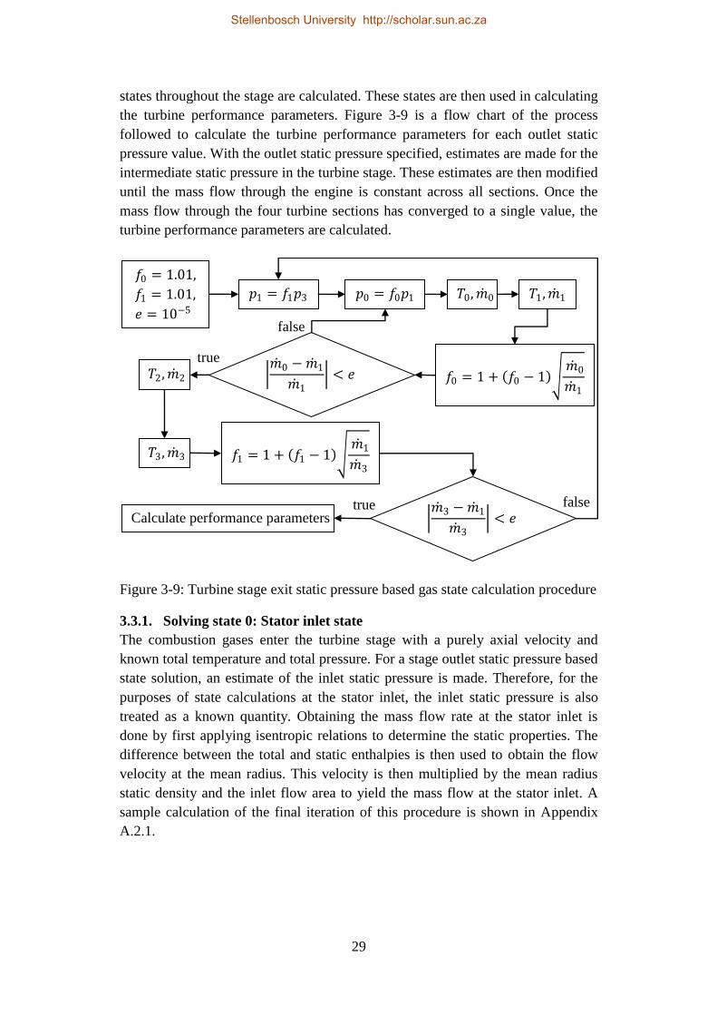
29

states throughout the stage are calculated. These states are then used in calculating

the turbine performance parameters. Figure 3-9 is a flow chart of the process

followed to calculate the turbine performance parameters for each outlet static

pressure value. With the outlet static pressure specified, estimates are made for the

intermediate static pressure in the turbine stage. These estimates are then modified

until the mass flow through the engine is constant across all sections. Once the

mass flow through the four turbine sections has converged to a single value, the

turbine performance parameters are calculated.

Figure 3-9: Turbine stage exit static pressure based gas state calculation procedure

3.3.1. Solving state 0: Stator inlet state

The combustion gases enter the turbine stage with a purely axial velocity and

known total temperature and total pressure. For a stage outlet static pressure based

state solution, an estimate of the inlet static pressure is made. Therefore, for the

purposes of state calculations at the stator inlet, the inlet static pressure is also

treated as a known quantity. Obtaining the mass flow rate at the stator inlet is

done by first applying isentropic relations to determine the static properties. The

difference between the total and static enthalpies is then used to obtain the flow

velocity at the mean radius. This velocity is then multiplied by the mean radius

static density and the inlet flow area to yield the mass flow at the stator inlet. A

sample calculation of the final iteration of this procedure is shown in Appendix

A.2.1.

𝑝1 = 𝑓1𝑝3 𝑝0 = 𝑓0𝑝1 𝑇0, �̇�0

�̇�0 − �̇�1

�̇�1 < 𝑒

𝑓0 = 1 + (𝑓0 − 1)√ �̇�0

�̇�1

𝑓0 = 1.01,

𝑓1 = 1.01,

𝑒 = 10−5

𝑇2, �̇�2

𝑇3, �̇�3 𝑓1 = 1 + (𝑓1 − 1)√ �̇�1

�̇�3

𝑇1, �̇�1

�̇�3 − �̇�1

�̇�3 < 𝑒

Calculate performance parameters false

false

true

true


30

3.3.2. Solving state 1: Stator exit state

In solving the stator exit state it is assumed that the flow conforms to the blade

angle as it leaves the trailing edge. Additionally, since the stator blades impart no

work to the flow and there is no heat loss, total enthalpy is conserved across this

blade row. Therefore the total temperature and enthalpy are known at the stator

exit.

The total pressure does not remain constant across the stator blade row due to total

pressure losses in the blade row. The relative total pressure loss coefficient, 𝑌, is

used to quantify these losses and is defined as the ratio of the relative total

pressure loss across a blade row to the exhaust relative dynamic pressure of the

blade row:

𝑌 =𝑝𝑡,𝑖𝑛

′ − 𝑝𝑡,𝑜𝑢𝑡′

𝑝𝑡,𝑜𝑢𝑡′ − 𝑝𝑜𝑢𝑡

. (3.32)

𝑌 is dependent on the blade geometry, the flow velocities and gas properties on

either side of the blade row. Therefore, since the flow field and gas properties are

also dependent on 𝑌, an iterative procedure is required to solve the exit state. An

initial guess of 𝑌 is made, facilitating the calculation of the exit state. The

resulting gas properties and flow field are then used to calculate a new total

pressure loss coefficient, and the process is repeated until the loss coefficient has

converged.

For the stator blade the relative total pressure loss coefficient becomes the

absolute total pressure loss coefficient, since the blade row is stationary. The

definition of 𝑌𝑆 is rearranged with the exhaust total pressure as the independent

variable.

𝑌𝑆 =𝑝𝑡0 − 𝑝𝑡1

𝑝𝑡1 − 𝑝1 → 𝑝𝑡1 =

𝑝𝑡0 + 𝑝1𝑌𝑆

𝑌𝑆 + 1 (3.33)

The isentropic relation for an ideal gas with varying specific heats is used to relate

the total-to-static specific temperature dependent entropy difference to the total-

to-static pressure ratio at any given state.

0 = 𝑠𝑡1𝑜 − 𝑠1

𝑜 − 𝑅𝑎𝑖𝑟 ln (𝑝𝑡1

𝑝1) (3.34)

Combining equations (3.33) and (3.34) yields the following expression for the

static specific temperature dependent entropy at the stator blade exit:

𝑠1𝑜 = 𝑠𝑡1

𝑜 − 𝑅𝑎𝑖𝑟 ln (𝑝𝑡0 + 𝑝1𝑌𝑆

𝑝1 + 𝑝1𝑌𝑆) (3.35)


31

Since the resulting value is only dependent on temperature, the static temperature

and the other static properties at state 1 can also be found. The static density and

flow velocity magnitude are obtained as is done for the stator inlet state. However,

unlike at the stator inlet state, the flow is not purely axial, since it conforms to the

exit blade angle. Therefore, the axial projection of the stator exit velocity is

multiplied by the corresponding gas density and flow area to yield the mass flow

rate at this position. The final iteration of a sample calculation for this procedure

is shown in Appendix A.2.2.

3.3.3. Solving state 2: Rotor inlet state

The blade height and mean radius may change between the stator exit state and

the rotor inlet state. The change in mean radius has an effect on the

circumferential velocity. This effect is modelled by enforcing conservation of

angular momentum. The angular momentum of a fluid particle at the mean radius

of state 1 is

𝐿1 = 𝐼1𝜔1 = 𝑚1𝑟𝑚12 𝜔1 = 𝑚1𝑟𝑚1𝐶𝜃1. (3.36)

The conservation of angular momentum dictates that a fluid particle at the mean

radius of state 2 should have the same angular momentum as of state 1. Assuming

equal masses for the particles at the two states, the relationship between the two

circumferential velocities can be shown to be

𝐶𝜃2 = 𝐶𝜃1 (𝑟𝑚1

𝑟𝑚2). (3.37)

The changes in the annulus dimensions also yield a change in the annular cross-

sectional area. This change in area is treated as either an isentropic nozzle or an

isentropic diffuser, depending on the sign. The total temperature and pressure

remain constant across such isentropic nozzles and diffusers. Therefore the total

properties at the rotor inlet are known.

The static properties at the rotor inlet are calculated using an initial guess of the

static gas density, and by assuming that the mass flow rate remains constant from

state 1 to state 2. This guessed value is then used to calculate the static

temperature and pressure at state 2, from which a new density is then calculated.

This process is repeated until the value of the static density at the rotor inlet has

converged, showing that the actual static properties have been calculated.

At state 2 the relative flow velocity and relative total gas properties become

relevant. The relative circumferential velocity at state 2 is given by:

𝑊𝜃2 = 𝐶𝜃2 − 𝑈2. (3.38)


32

Since the motion of the blade is perpendicular to the axial direction, there is no

difference between the absolute and relative axial-flow velocity. The relative flow

velocity at state 2 is therefore given by

𝑊2 = √𝐶𝑧22 + 𝑊𝜃2

2 . (3.39)

This relative velocity is used to calculate the relative total gas enthalpy and

pressure at state 2. A sample calculation of the final iteration in calculating state 2

is shown in Appendix A.2.3.

3.3.4. Solving state 3: Rotor exit state

The procedure for solving the rotor exit state is similar to the procedure for

solving the stator exit state. The main difference between the two cases is that,

since the rotor extracts work from the flow, the total enthalpy changes between

state 2 and state 3. However, it can be shown that for a constant radius axial-flow

blade row the relative total enthalpy remains constant across the blade row

(Dixon, 1998). Therefore the same approach for determining the stator exit flow

properties is used, with all the total properties being substituted by relative total

properties. The mass flow rate is then calculated using the axial projection of the

relative rotor exit velocity. The absolute velocity and total flow properties are then

calculated from the static and relative properties and velocity. The final iteration

of this procedure is shown in full as a sample calculation in Appendix A.2.4.

3.3.5. Calculating the turbine stage performance parameters

The performance parameters of a turbine stage operating at a specified total-to-

static pressure ratio are the total-to-total pressure ratio, the mass flow rate and the

total-to-total efficiency. The mass flow rate is calculated in the last state

calculation iteration and the total-to-total pressure ratio can also be obtained

directly from these calculated values. The total-to-total efficiency, however, is

calculated from the equation:

𝜂𝑡𝑡 =ℎ𝑡0 − ℎ𝑡3

ℎ𝑡0 − ℎ𝑡3,𝑖𝑑𝑒𝑎𝑙 (3.40)

The ideal rotor exit total enthalpy is calculated using isentropic relations and

assuming the total-to-total pressure ratio remains unchanged. A sample

calculation of this procedure is shown in Appendix A.2.5.

3.4. Results of empirical performance analysis

The performance analysis procedure described in section 3.3 is applied to the

reverse engineered turbine of the BMT 120 KS engine. The inlet total pressure

and total temperature is taken to be 308,3 kPa and 1119 K respectively and

performance curves are generated for four rotor speeds. These curves of total-to-


33

total efficiency and actual-to-design mass flow rate ratio are shown in Figure

3-10. It can be seen that the peak total-to-total efficiency moves from a lower to a

higher pressure ratio as the rotational speed of the turbine is increased. The same

trend is also visible for the peak mass flow rate through the turbine. These trends

correspond well to those on a similar turbine performance map published by

Cohen et al. (1996). However, it can also be seen that the mass flow rate predicted

by the empirical performance analysis is substantially lower than the design mass

flow rate of the BMT 120 KS turbine of 0,29 kg/s, given in Table 4-2. This

discrepancy in the mass flow rate prediction suggests that assumptions made in

the analysis procedure are inaccurate for the BMT 120 KS turbine. The

assumption of the mean radius mass flux being equal to the average mass flux at a

given cross section is a likely source of this inaccuracy, as suggested by Cohen et

al. (1996).

3.5. Conclusion

A mean radius performance analysis procedure using empirical loss correlations

was developed. The empirical loss model was described and the analysis

procedure for calculating the performance of a turbine under specified conditions

was proposed. This procedure was applied to an existing turbine design and a

turbine performance map was generated. This performance map compares well

with the trends shown in similar charts in literature, even though the mass flow

rate was substantially under predicted.


34

Figure 3-10: BMT 120 KS turbine empirical performance map at Tt0 = 1119 K, pt0

= 308300 Pa

-1.2

-1

-0.8

-0.6

-0.4

-0.2

0

0.2

0.4

0.6

0.8

1

0

0.2

0.4

0.6

0.8

1

1.2

1.4

1.6

1.8

2

2.2

1 1.2 1.4 1.6 1.8 2 2.2

To

tal-

to-t

ota

l eff

icie

ncy

, η

tt

Mas

s fl

ow

rat

e ra

tio

, ṁ

/ṁd

esig

n

Total-to-total pressure ratio, pt0/pt3

140 krpm

120 krpm

100 krpm

80 krpm


35

4. Turbine design process

4.1. Introduction

This section describes the procedure for designing an axial-flow turbine to match

the requirements of an existing micro gas turbine engine. Designing a turbine for

an existing engine simplifies the evaluation of the generated turbine design, since

the existing turbine design provides a clear baseline to which any new design can

be compared. Once the turbine performance requirements of the existing engine

have been determined, the design process is identical to the case where a turbine

for a new engine is designed.

Firstly the assumptions and primary design decisions are stated; whereafter the

turbine design parameters are identified. The values of these parameters are

deduced from measurements and test results of the existing engine. These

parameters are then used to calculate the mean radius gas velocity vectors before

and after each blade row and to make a preliminary stage efficiency estimate. The

gas velocity magnitudes are then used along with the efficiency estimate to

approximate the mean radius thermodynamic gas properties before and after each

blade row. Once the gas properties, specifically the gas density, are known

throughout the stage, the annular flow passage is sized to pass the design mass

flow rate. The mean radius blade profiles are then also calculated, thus enabling

the empirical loss model to predict the total pressure loss coefficient of each blade

row. The properties of the gas throughout the turbine stage are then recalculated

using these loss coefficients, instead of the preliminary efficiency estimates.

These properties are then used to finalise the sizing of the annular flow passage.

Once the geometry of the flow passage is finalised, the blade profiles from root to

tip can be generated. This profile information is then converted to three-

dimensional models of each blade row.

4.2. Assumptions and design decisions

4.2.1. Machine type and geometry

The existing micro gas turbine engine, for which the new turbine is to be

designed, is fitted with a single stage axial-flow turbine. The stage consists of a

shrouded stator blade row and an un-shrouded rotor blade row. This configuration

is adopted for the new design to simplify integration into the existing engine.

Figure 4-1 shows a turbine stage with the adopted configuration. Part of the

shrouded stator is removed for clarity.


36

Figure 4-1: Turbine stage configuration

The mean radius of the turbine stage is chosen to remain constant throughout the

turbine. Therefore, when the properties of the flow along the mean radius stream

sheet are calculated, the radius of the flow remains constant before and after a

blade row. This invariance in radii causes the mean radius relative stagnation

enthalpy to be conserved across both stationary and rotating blade rows.

4.2.2. Swirl velocity distributions

A free vortex swirl velocity distribution is chosen for the exit to the stator blade

row. This is the most common choice of swirl velocity vortex type for axial-flow

gas turbines (Aungier, 2006), since it minimizes kinetic energy losses associated

with vortical motion in the gas (Baskharone, 2006). This choice results in both the

axial components of the gas velocities and the blade work per unit mass of flow

being invariant with radius. The flow entering and leaving the turbine stage is

chosen to be purely axial. The swirl velocity distribution of the entering flow

comes from the combustion chamber and is therefore neither steady, nor uniform.

Therefore, the assumption of a purely axial velocity is made to average out the

fluctuating flow. The axial turbine exit flow velocity is chosen to minimise the

total pressure lost due to the exit flow kinetic energy.


37

4.2.3. Streamwise constant axial velocity

The density of the gas passing through a turbine decreases from inlet to outlet.

The accompanying increase in specific volume flow rate leaves the designer with

two options. Firstly, the flow passage can have a constant cross-sectional area.

The constant flow area would require continuity to be enforced by an increase in

gas axial velocity from inlet to outlet. Such an increase in axial velocity may,

however, cause unacceptably high relative Mach numbers on the trailing edge of

the rotor row. Therefore the second option is to have the cross-sectional area of

the flow passage increase from inlet to outlet. This configuration would allow the

the specific volume flow rate to increase without the risk of excessively high axial

velocities and the accompanying choking danger.

For the present design a constant axial velocity is specified throughout the turbine

stage. This specification alleviates the danger of excessively high blade exit Mach

numbers and simplifies the calculation of the mean radius gas properties

throughout the turbine stage. The resulting diverging hub and shroud walls are

shown in Figure 4-2 where the flow area increases from position 0 at the inlet to

position 3 at the outlet.

4.3. Design parameters

The parameters that dictate the design of the turbine can be divided into three

categories. These categories are:

the constraints placed on the geometry of the turbine stage,

the thermo-physical properties of the gases exiting the combustion

chamber,

and the turbine performance required to drive the compressor at the design

point.

In this section the variables relevant to each parameter category are identified, and

the procedure for determining the values of these variables is explained.

4.3.1. Geometrical constraints

In a case where a turbine is designed to be retrofitted to an existing jet engine

certain geometrical constraints must be met. These constrains consist of limits on

the total external turbine stage dimensions and limitations placed on the stage inlet

geometry. Figure 4-2 also shows these limiting dimensions.


38

𝑧𝑠𝑡𝑎𝑔𝑒

𝑏𝑧,𝑠𝑡𝑎𝑡𝑜𝑟 𝑏𝑧 ,𝑟𝑜𝑡𝑜𝑟 ∆𝑧

𝑡𝑤𝑎𝑙𝑙

𝑟 𝑠,𝑚

𝑎𝑥

𝑟 𝑠0

𝑟 ℎ0 𝑟 𝑚

𝑒𝑎𝑛

0 1 2 3

Figure 4-2: Geometrical constrains and turbine axial position definition

Total external stage dimensions

A limited amount of space within the housing of the engine is available for the

turbine stage. Therefore, the maximum external diameter and stage length are

limited. The limit on the external diameter, 𝑑𝑚𝑎𝑥, translates into a limit on the

maximum shroud inner radius, 𝑟𝑠,𝑚𝑎𝑥 , and wall thickness, 𝑡𝑤𝑎𝑙𝑙. This limitation

can be expressed as:

The limit on the total stage length allows for the fixing of the stator and rotor

blade axial chords. In accordance with accepted design practice, the axial gap

between the two blade rows, ∆𝑧, is then chosen to be 50% of the average of the

two axial blade chords (Cohen, et al., 1996):

This then yields a total stage length of:

(𝑟𝑠,𝑚𝑎𝑥 + 𝑡𝑤𝑎𝑙𝑙) ≤ 𝑑𝑚𝑎𝑥/2 . (4.1)

∆𝑧 = 0.5 (𝑏𝑧,𝑠𝑡𝑎𝑡𝑜𝑟 + 𝑏𝑧,𝑟𝑜𝑡𝑜𝑟

2). (4.2)

𝑧𝑠𝑡𝑎𝑔𝑒 = 𝑏𝑧,𝑠𝑡𝑎𝑡𝑜𝑟 + 𝑏𝑧,𝑟𝑜𝑡𝑜𝑟 + ∆𝑧. (4.3)


39

Stage inlet geometry

The inlet geometry of the turbine stage must be compatible with the exit geometry

of the preceding combustion chamber. Therefore the turbine stage inlet annular

flow path section must fit within the annular exit flow path section of the

combustion chamber. This limitation translates into a maximum allowable inlet

shroud radius and a minimum allowable inlet hub radius.

Values for the geometrical design parameters are chosen to meet the

aforementioned constraints. The values for the present design are shown in Table

4-1.

Table 4-1: Geometrical design parameter selections

4.3.2. Inlet gas properties

The inlet gas properties of a turbine stage are obtained indirectly from compressor

test results. Experimental work was done on the present engine by Krige (2012).

The performance data obtained from this experimental work is shown in Table

4-2.

Table 4-2: Current engine experimental test data at 120 krpm. (Krige, 2012)

Geometrical parameter name Parameter value

Stage inlet hub radius, 𝑟ℎ0 23,5 mm

Stage inlet shroud radius, 𝑟𝑠0 31,5 mm

Stator blade axial chord, 𝑏𝑧,𝑠𝑡𝑎𝑡𝑜𝑟 9 mm

Rotor blade axial chord, 𝑏𝑧,𝑟𝑜𝑡𝑜𝑟 7 mm

Parameter name Parameter value

Air mass flow rate, �̇�𝑎𝑖𝑟 0,29 kg/s

Fuel mass flow rate, �̇�𝑓𝑢𝑒𝑙 0,0054 kg/s

Compressor inlet total temperature, 𝑇𝐶,𝑡,𝑖𝑛 289 K

Compressor inlet total pressure, 𝑝𝐶,𝑡,𝑖𝑛 101 kPa

Compressor exit total pressure, 𝑝𝐶,𝑡,𝑜𝑢𝑡 310 kPa

Compressor total-to-total efficiency, 𝜂𝐶,𝑡𝑡 85 %

Turbine exit total temperature, 𝑇𝑇,𝑡,𝑜𝑢𝑡 1009 K


40

The compressor inlet temperature, efficiency and pressure ratio are used to

calculate the amount of work imparted to the flow by the compressor of the jet

engine. This compressor work can then be multiplied by the air mass flow rate to

obtain the mechanical power required to drive the compressor. Assuming

negligible mechanical losses, the turbine is then required to extract the same

amount of power from the flow to drive the compressor. The mass flow rate

through the turbine includes both the compressor air mass flow rate and the fuel

mass flow rate. Therefore, the turbine work per unit mass is found by dividing the

compressor power by the turbine mass flow. Adding the turbine work per unit

mass to the turbine outlet total enthalpy yields the turbine stage inlet total

enthalpy, and hence the inlet total temperature. The turbine inlet total pressure is

obtained by assuming a zero total pressure loss through the combustion chamber.

Therefore, the total pressure at the turbine inlet equals the total pressure at the

compressor exit. The turbine inlet gas properties are shown in Table 4-3. The

procedure for calculating the turbine inlet total pressure and temperature is shown

in Appendix B.1.

Table 4-3: Turbine inlet gas properties

4.3.3. Turbine performance requirements

The performance requirements of the turbine at the design points consist of the

power output, the rotational speed and mass flow rate. At the design point, the

turbine must drive the compressor at 120,000 revolutions per minute. Therefore,

the design point is at the same operating conditions as the test data of Table 4-2.

Therefore, the mass flow rate and the turbine power output are required to equal

the values used to calculate the turbine inlet total temperature.

Non-dimensional forms of the performance requirement are calculated at the

mean radius for use during the design process. The non-dimensional flow

coefficient, work coefficient and reaction ratio, as defined in Appendix B.3, are

obtained from the turbine performance requirements and the chosen geometrical

design parameters. The shapes of the turbine stage velocity triangles are

determined by the values of these non-dimensional parameters (Wilson, 1987).

The non-dimensional performance parameters and dimensional performance

requirements are shown in Table 4-4. A numerical example of the procedure used


Turbine inlet total temperature, 𝑇𝑡0 1119 K

Turbine inlet total pressure, 𝑝𝑡0 310 kPa


41

to calculate the non-dimensional performance parameters is shown in Appendix

B.2.

Table 4-4: Turbine performance requirements

4.4. Mean radius gas velocity triangles and efficiency estimate

4.4.1. Calculating the mean radius gas velocity triangles

The mean radius gas velocity vectors are dependent on the specified stage work

and flow coefficients, as well as the absolute stage inlet and exit flow angles. The

unknown absolute and relative gas angles are calculated using equations (4.4) and

(4.5) and equations (4.6) and (4.7) respectively.

The constant mean radius axial gas velocity component is calculated from the

flow coefficient and the blade speed in equation (4.8).


Turbine power output, 𝑃𝑇 37 kW

Turbine mass flow rate, �̇�𝑇 0,29 kg/s

Turbine rotational speed, 𝑁𝑇 or 𝜔𝑇 120 krpm or 12 600 rad/s

Turbine flow coefficient, 𝜙𝑚𝑒𝑎𝑛 0,69

Turbine work coefficient, 𝜓𝑚𝑒𝑎𝑛 1,06

Turbine reaction ratio, 𝑅𝑚𝑒𝑎𝑛 0,47

𝛼1,𝑚𝑒𝑎𝑛 = atan (1 − 𝑅𝑚𝑒𝑎𝑛 +

𝜓𝑚𝑒𝑎𝑛

2𝜙𝑚𝑒𝑎𝑛

) (4.4)

𝛼2,𝑚𝑒𝑎𝑛 = 𝛼1,𝑚𝑒𝑎𝑛 (4.5)

𝛼′2,𝑚𝑒𝑎𝑛 = atan (−𝑅𝑚𝑒𝑎𝑛 −



) (4.6)

𝛼′3,𝑚𝑒𝑎𝑛 = atan (−𝑅𝑚𝑒𝑎𝑛 +



) (4.7)


42

The absolute and relative gas velocity magnitudes at any position, 𝑖, along the

turbine stage are given by equations (4.9) and (4.10) respectively. The derivation

of equations (4.4) to (4.7) is explained and the resulting numerical values of the

stage mean radius gas velocities are shown in Appendix B.3.

𝐶𝑖,𝑚𝑒𝑎𝑛 = 𝐶𝑧,𝑚𝑒𝑎𝑛/ cos 𝛼𝑖,𝑚𝑒𝑎𝑛 (4.9)

𝑊𝑖,𝑚𝑒𝑎𝑛 = 𝐶𝑧,𝑚𝑒𝑎𝑛/ cos 𝛼′𝑖,𝑚𝑒𝑎𝑛 (4.10)

4.4.2. Preliminary efficiency estimate

The purpose of the preliminary design process is to produce candidate designs for

the detail design process. Therefore, it would be helpful to determine whether or

not a preliminary design is likely to yield acceptable performance. This is

accomplished by obtaining a stage efficiency estimate from a standardised

efficiency chart.

The Smith chart (Smith, 1965) is a standardised efficiency chart that is widely

accepted as feasible for use during preliminary turbine design. It is a plot of total-

to-total efficiency contours on axes of flow coefficient and work coefficient.

Aungier (2006) made an empirical correlation from the Kacker and Okapuu

(1981) data that shows good agreement with the Smith chart. It yields an

expression for the total-to-total efficiency of a stage as a function of its flow and

work coefficients as shown in equations (4.11) to (4.14).

This correlation assumes a reaction ratio of 50%, no tip clearance and moderate to

high blade aspect ratios. Aungier (2006), however, corrects for these assumptions

by using a standard tip clearance approximation,

𝐶𝑧,𝑚𝑒𝑎𝑛 = 𝜙𝑚𝑒𝑎𝑛𝑈𝑚𝑒𝑎𝑛 (4.8)

𝜙𝑜𝑝𝑡 = 0.375 + 0.25𝜓𝑚𝑒𝑎𝑛 (4.11)

𝜂𝑜𝑝𝑡

= {0.913 + 0.103𝜓𝑚𝑒𝑎𝑛 − 0.0854𝜓𝑚𝑒𝑎𝑛

2 + 0.0154𝜓𝑚𝑒𝑎𝑛3 , 𝜓𝑚𝑒𝑎𝑛 ≤ 2.8

1.01 − 0.05𝜓𝑚𝑒𝑎𝑛, 𝜓𝑚𝑒𝑎𝑛 > 2.8 (4.12)

𝐾1 = {

0.375 − 0.125𝜓𝑚𝑒𝑎𝑛, 𝜓𝑚𝑒𝑎𝑛 ≤ 2.20.22

𝜓𝑚𝑒𝑎𝑛, 𝜓𝑚𝑒𝑎𝑛 > 2.2

(4.13)

𝜂0 = 𝜂𝑜𝑝𝑡 − 𝐾1(𝜙𝑚𝑒𝑎𝑛 − 𝜙𝑜𝑝𝑡) (4.14)


43

and an aspect ratio correction that is also dependent on the reaction ratio,

Therefore, the corrected total-to-total efficiency is given by

This initial efficiency estimate is to be used in the preliminary calculation of the

gas states along the mean radius throughout the turbine stage. In addition to the

turbine stage total-to-total efficiency, the nozzle efficiency of the stator blade row

is also required for a gas states calculation. A stator blade row nozzle efficiency of

94 % is assumed for the preliminary state calculations of the following section.

4.5. Gas states calculation

The thermodynamic states of the gases passing through the engine are calculated

at four locations along the mean radius of the turbine stage. These locations

correspond to the inlet and outlet planes of the stator and rotor blades rows. The

knowledge of the gas states enables the sizing of the flow path at the different

locations and is also necessary for the empirical performance analysis of each

blade row. It also enables the mean radius flow Mach numbers to be calculated.

The gas states are calculated using two independent procedures. Initially, the

states are calculated using the preliminary turbine stator blade row nozzle

efficiency and turbine stage total-to-total efficiency estimates to account for the

entropy increase through the stage. These calculations are used to generate the

Mollier diagram of the turbine stage shown in Figure 4-3. In Figure 4-3 the points

denoted by 1s and 3s are respectively the stator exit and rotor exit ideal states. The

points denoted 3ss refer to the ideal stage exit states.

The results of this initial state calculation are used as an input into the empirical

loss model of Section 3. The empirical loss model yields relative total pressure

loss coefficients that are then used in the gas states calculations of all subsequent

design iterations. A numerical example of the gas states calculation, using the

converged values of the relative total pressure loss coefficients of the two blade

rows, is shown in Appendix B.4.

𝐾2 =𝛿

𝑟𝑚𝑒𝑎𝑛 + 𝐻0/2 , (4.15)

𝑋 = 𝐻0(0.4 + 0.5𝑅𝑚𝑒𝑎𝑛). (4.16)

𝜂𝑡𝑡 = 𝜂0 [1 + 0.93𝐾2 (𝑟𝑚𝑒𝑎𝑛

𝐻0) (1 +

0.5𝐻0

𝑟𝑚𝑒𝑎𝑛)

2

] 𝑋0.05+0.04𝑅𝑚𝑒𝑎𝑛 . (4.17)


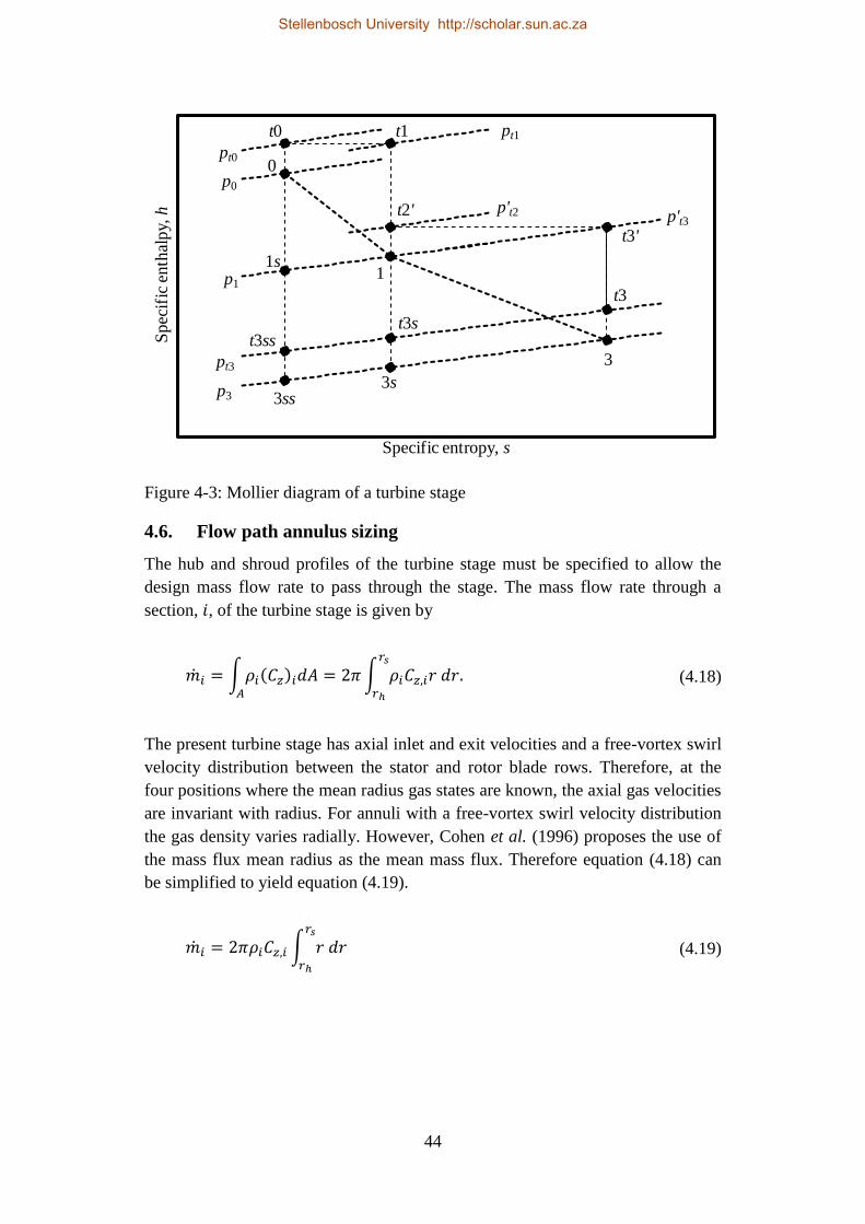
44

Figure 4-3: Mollier diagram of a turbine stage

4.6. Flow path annulus sizing

The hub and shroud profiles of the turbine stage must be specified to allow the

design mass flow rate to pass through the stage. The mass flow rate through a

section, 𝑖, of the turbine stage is given by

The present turbine stage has axial inlet and exit velocities and a free-vortex swirl

velocity distribution between the stator and rotor blade rows. Therefore, at the

four positions where the mean radius gas states are known, the axial gas velocities

are invariant with radius. For annuli with a free-vortex swirl velocity distribution

the gas density varies radially. However, Cohen et al. (1996) proposes the use of

the mass flux mean radius as the mean mass flux. Therefore equation (4.18) can

be simplified to yield equation (4.19).

t0

0

t1

1

t2'

1s

t3

3

t3'

3s3ss

t3st3ss

pt0

p't3

p0

pt1

p't2

p1

pt3

p3

Spec

ific

enth

alpy,

h

Specific entropy, s

�̇�𝑖 = ∫𝜌𝑖(𝐶𝑧)𝑖𝑑𝐴

𝐴

= 2𝜋 ∫ 𝜌𝑖𝐶𝑧,𝑖𝑟 𝑑𝑟𝑟𝑠

𝑟ℎ

. (4.18)

�̇�𝑖 = 2𝜋𝜌𝑖𝐶𝑧,𝑖 ∫ 𝑟 𝑑𝑟𝑟𝑠

𝑟ℎ

(4.19)


45

The axial velocity and mean radius are chosen to remain constant throughout the

stage. These assumptions also simplify equation (4.19), allowing it to be re-

ordered to yield the expression for the blade height in equation (4.20).

The stage inlet hub and shroud radii are already specified in Table 4-1. The hub

and shroud radii at the three remaining positions are then obtained from the mean

radius and the blade heights calculated using equation (4.20). These radii describe

the hub and shroud contours at four sections along the length of the stage. The

radii at these points are interpolated to yield piece-wise linear hub and shroud

contours, similar to the contours shown in Figure 4-2.

4.7. Blade profile construction

The gas velocity triangles have been calculated to yield the desired turbine stage

performance. However, turbine blades are needed to produce a flow field that

conforms to these velocity triangles. These blades require cross-sectional profiles

that impart the appropriate amount of swirl to the moving gases, whilst causing

minimal flow obstruction and entropy generation. The blade cross sections are

designed by first evaluating several general geometric blade row parameters using

empirical correlations. A thickness-camber scheme to describe the blade profiles

is chosen because of the low number of variables required to define an airfoil

shape (Wesssels, et al., 2012). The geometric parameters are then used to generate

blade camber line curves with inlet and outlet angles that conform to the desired

flow field. A distribution of the blade thickness along the camber line is then

chosen. These thickness distributions are then added perpendicularly to both the

pressure and suction sides of the camber line curves. The resulting curves form

the edges of the suction and pressure surfaces on the blade profile.

4.7.1. Blade row geometric parameters

Different parameters are used to characterise the geometry of a blade row. By

adjusting these parameters and the ratios between pairs of these parameters the

shape of a blade profile can be controlled. Therefore, an attempt is made to find

near-optimal values of the blade parameters for the specified design parameters.

Determining the optimal pitch-to-chord ratio

The pitch-to-chord ratio of a blade row is a measure of the size and number of

blades in the blade row. When large flow deflections are required, lower pitch-to-

𝐻𝑖 =�̇�𝑖

2𝜋𝑟𝑚𝑒𝑎𝑛𝐶𝑧𝜌𝑖 (4.20)


46

chord ratios are required than when smaller flow deflections are required. The size

and number of the blades can however not increase indefinitely due to the

blockage caused in the flow passage and other geometrical and material

constraints. Therefore an optimal pitch-to-chord ratio is required to ensure that a

blade row is capable of achieving the required flow deflection, whilst not causing

undue flow passage blockage.

The optimal pitch-to-chord ratio is determined by applying an empirical

correlation that uses the generic blade angle convention (Ainley & Mathieson,

1951). This correlation works from the assumption that any turbine blade can be

reconstructed as a weighted combination of a pure nozzle blade and an impulse

blade. The weighting is done using the gas deflection ratio, 𝜉, as defined in

equation (3.5). Ainley and Mathiesson (1951) published correlations for the

optimal pitch-to-chord ratios for pure nozzle blades and impulse blades. These

correlations are used in the empirical performance analysis of Section 3 and

shown in Figure 3-2. The resulting optimal pitch-to-chord ratios for a range of

turbine blade inlet and outlet angles are shown in Figure 4-4.

Figure 4-4: Optimal pitch to chord ratio for different combinations of blade inlet

and exit angles

Determining the blade pitch, chord and stagger angle

The next step in designing turbine blades is to determine the values of various

geometric blade parameters. These parameters are primarily the blade stagger

angle, the blade pitch and chord length. These primary blade parameters are also

0.5

0.6

0.7

0.8

0.9

1

1.1

1.2

20 30 40 50 60 70

Opti

mal

pit

ch-t

o-c

hord

rat

io,

(s/c

) op

t

Exit blade angle, αb1, degrees

nozzle blade

impulse blades

βb0 = 110

80

70 60

40


47

related to the blade gauge angle, deviation angle and the number of blades. An

empirical correlation from Aungier (2006) is used to estimate the optimal values

of these three parameters. The throat-pitch ratio is given as:

(𝑜

𝑠) = 𝐹𝐴𝑅 sin(𝛽1 − 𝛿). (4.21)

The stream sheet area ratio correction is given by:

𝐹𝐴𝑅 = 0.8 + 0.2 (𝜌0𝐶𝑧0

𝜌1𝐶𝑧1). (4.22)

The deviation angle, defined in equation (4.23), is a function of the zero relative

exit Mach number deviation angle, given by equation (4.24), and the relative exit

Mach number.

𝛿 = {𝛿0, 𝑀1

′ ≤ 0.5

𝛿0[1 − 10(2𝑀1′ − 1)3 + 15(2𝑀1

′ − 1)4 − 6(2𝑀1′ − 1)5], 𝑀1

′ > 0.5 (4.23)

𝛿0 = sin−1 {(𝑜

𝑠) [1 + (1 −

𝑜

𝑠) (

𝛽𝑔

90°)

2

]} − 𝛽𝑔 (4.24)

The gauge angle and stagger angle are given by equations (4.25) and (4.26)

respectively.

𝛽𝑔 = sin−1(𝑜/𝑠) (4.25)

𝛾 =(180° − 𝛽0 + 1.5𝛽𝑔)

2.5 (4.26)

The blade chord is then calculated from the specified axial chord and the

calculated stagger angle. This allows the blade pitch to be calculated by also using

the pitch to chord ratio. Finally the number of blades is calculated from the blade

pitch and the mean radius. The resulting value is rounded to the nearest prime

integer or prime integer double. The use of a prime number of blades minimises

the number of cyclic disturbance frequencies a blade would be subjected to during

operation. These profile geometrical parameters are highly interrelated. Therefore

an iterative procedure is used to satisfy all the relationships. A numerical example

of calculating the rotor blade row geometrical parameters is shown in Appendix

B.5.

4.7.2. Blade camber line

The known values of the blade chord length and the stagger angle yield the

relative positions of the leading and trailing edge points of the blade profile. These


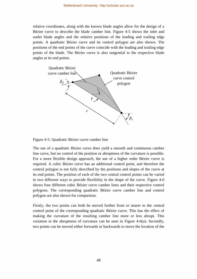
48

relative coordinates, along with the known blade angles allow for the design of a

Bézier curve to describe the blade camber line. Figure 4-5 shows the inlet and

outlet blade angles and the relative positions of the leading and trailing edge

points. A quadratic Bézier curve and its control polygon are also shown. The

positions of the end points of the curve coincide with the leading and trailing edge

points of the blade. The Bézier curve is also tangential to the respective blade

angles at its end points.

0

1

Quadratic Bézier

curve camber line

Quadratic Bézier

curve control

polygon

Figure 4-5: Quadratic Bézier curve camber line

The use of a quadratic Bézier curve does yield a smooth and continuous camber

line curve, but no control of the position or abruptness of the curvature is possible.

For a more flexible design approach, the use of a higher order Bézier curve is

required. A cubic Bézier curve has an additional control point, and therefore the

control polygon is not fully described by the positions and slopes of the curve at

its end points. The position of each of the two central control points can be varied

in two different ways to provide flexibility in the shape of the curve. Figure 4-6

shows four different cubic Bézier curve camber lines and their respective control

polygons. The corresponding quadratic Bézier curve camber line and control

polygon are also shown for comparison.

Firstly, the two points can both be moved further from or nearer to the central

control point of the corresponding quadratic Bézier curve. This has the effect of

making the curvature of the resulting camber line more or less abrupt. This

variation in the abruptness of curvature can be seen in Figure 4-6(a). Secondly,

two points can be moved either forwards or backwards to move the location of the


49

camber line curvature towards either the leading or trailing edge points. This

movement of the curvature position is shown in Figure 4-6(b).

(b) (a)

Quadratic Bézier

curve control

polygon

Quadratic Bézier

curve camber line

Cubic Bézier

curve camber

line

Cubic Bézier

curve control

polygon

Figure 4-6: Variation of cubic Bézier curve camber line shapes

4.7.3. Blade thickness profile

A blade thickness profile is added to the existing camber line curve. A T6 profile,

a thickness profile commonly used for gas turbine blades (Cohen, et al., 1996), is

used as a starting point for the thickness distribution. A fifth-degree Bézier curve

is then used to create a curve that approximates the T6 profile definition points.

The use of higher-order Bezier curves enforces the third-order continuity that

keeps the Mach number distribution smooth, resulting in lower trailing edge

losses (Korakianitis & Papagiannidis, 1993). The Bézier curve and its control

polygon, together with the T6 profile definition points are shown in Figure 4-7.

The central four control points of the Bézier curve can be moved around to

modify the blade thickness distribution. The first and fourth control points can

only be moved transversely, enabling control of the leading and trailing edge

thickness. In Figure 4-7 it can be seen that the fourth control point is moved to

yield a trailing edge that is thicker than what the T6 defining points describe.

Once the blade profile camber line and thickness distribution have been

determined, the thickness distribution is applied to the camber line. The resulting

blade profile conforms to the flow field for which it was designed.


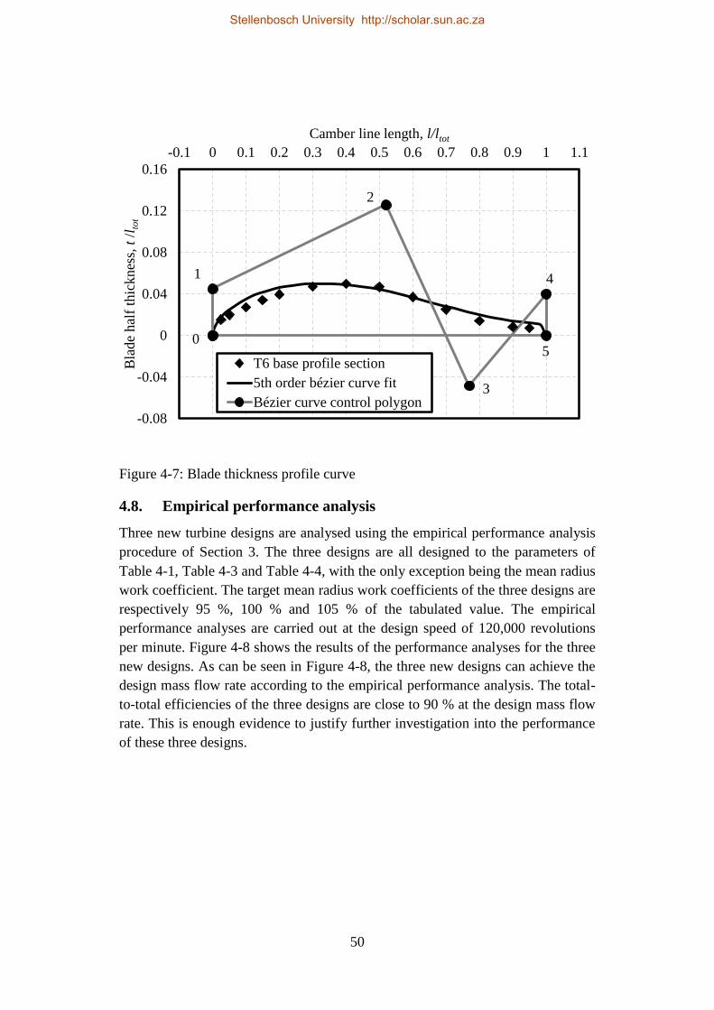
50

Figure 4-7: Blade thickness profile curve

4.8. Empirical performance analysis

Three new turbine designs are analysed using the empirical performance analysis

procedure of Section 3. The three designs are all designed to the parameters of

Table 4-1, Table 4-3 and Table 4-4, with the only exception being the mean radius

work coefficient. The target mean radius work coefficients of the three designs are

respectively 95 %, 100 % and 105 % of the tabulated value. The empirical

performance analyses are carried out at the design speed of 120,000 revolutions

per minute. Figure 4-8 shows the results of the performance analyses for the three

new designs. As can be seen in Figure 4-8, the three new designs can achieve the

design mass flow rate according to the empirical performance analysis. The total-

to-total efficiencies of the three designs are close to 90 % at the design mass flow

rate. This is enough evidence to justify further investigation into the performance

of these three designs.

-0.08

-0.04

0

0.04

0.08

0.12

0.16

-0.1 0 0.1 0.2 0.3 0.4 0.5 0.6 0.7 0.8 0.9 1 1.1

Bla

de

hal

f th

icknes

s, t

/l t

ot

Camber line length, l/ltot

T6 base profile section

5th order bézier curve fit

Bézier curve control polygon

2

1

0

3

4

5


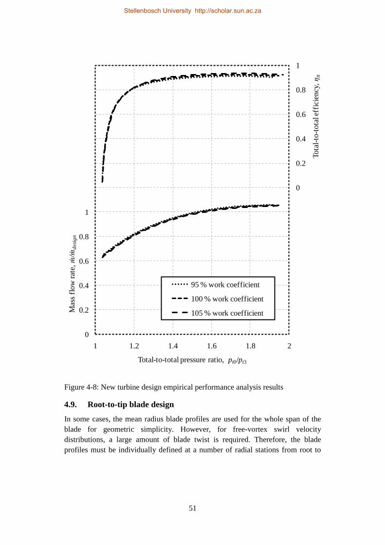
51

Figure 4-8: New turbine design empirical performance analysis results

4.9. Root-to-tip blade design

In some cases, the mean radius blade profiles are used for the whole span of the

blade for geometric simplicity. However, for free-vortex swirl velocity

distributions, a large amount of blade twist is required. Therefore, the blade

profiles must be individually defined at a number of radial stations from root to

-1.2

-1

-0.8

-0.6

-0.4

-0.2

0

0.2

0.4

0.6

0.8

1

0

0.2

0.4

0.6

0.8

1

1.2

1.4

1.6

1.8

2

2.2

1 1.2 1.4 1.6 1.8 2

To

tal-

to-t

ota

l eff

icie

ncy

, η

tt

Mas

s fl

ow

rat

e, ṁ

/ṁd

esig

n

Total-to-total pressure ratio, pt0/pt3

95 % work coefficient




52

tip. This is done by first calculating the flow angles at each radial station and then

calculating the profile geometrical parameters. The blade profile for each radial

station is then calculated. These profiles can then be stacked along an appropriate

stacking axis to generate a three-dimensional blade model.

4.9.1. Free-vortex velocity triangles

The gas velocity triangles for the stream sheet of each radial station are calculated

using free-vortex theory. For a free-vortex stator design the circumferential

component of the absolute flow velocity between the two blade rows is inversely

proportional to the radius of the radial station. Since the mean radius gas velocity

triangles have been fixed, the free-vortex constant is already available. Free-

vortex theory also dictates that the axial velocity remains constant with radius.

Therefore, since the mean radius velocity vectors are known, the velocity vectors

at the other radial station can be readily calculated.

4.9.2. Radial station blade profiles

With the flow velocity triangles at a radial station known, the blade profile

parameters can be calculated. The same procedure used to calculate the mean

radius profile can be used. However, the blade pitch is determined by the radius of

the radial station, since the number of blades has already been specified.

The blade profile camber lines are calculated as before from the blade inlet and

outlet angles, stagger angles and chords for each radial station. The pressure and

suction surface edges are also calculated as a combination of the camber line

curves and the thickness distribution as before. The thickness distribution

calculations, however, differ in that a blade taper factor dependent on the radius is

introduced. This factor enables the thickness of the blade to be reduced from root

to tip. Such a reduction in thickness, or taper, can be used to decrease the amount

of stress in the root of the blade during operation. For the present designs, the

blade taper factor is chosen to result in the blade roots and tips being respectively

25% thicker and 25% thinner than the mean radius profiles.

4.9.3. Blade profile stacking axis

The blade profile of each radial station must somehow be stacked to form a three-

dimensional blade surface. To minimise bending stresses on the rotating blade, the

blade sections are stacked on a radial line through the sectional centre of gravity

of each profile. Figure 4-9 on the next page shows how the profiles at five radial

stations of a rotor blade have been stacked to create a three dimensional blade

surface.


53

Figure 4-9: Rotor blade profile stacking

4.10. Conclusion

This section describes the design process of a replacement turbine for an existing

micro jet engine. The process for obtaining the design parameters is shown and a

method for designing a turbine to meet those design parameters is presented. The

method is used to generate three candidate design and these designs are subjected

to an empirical performance analysis. The results of the analysis are encouraging,

thus justifying further analysis of the designs.


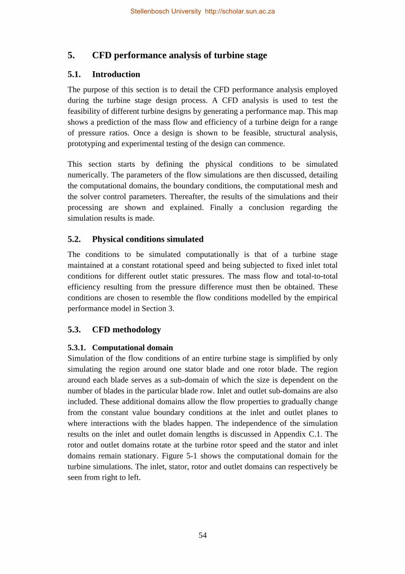
54

5. CFD performance analysis of turbine stage

5.1. Introduction

The purpose of this section is to detail the CFD performance analysis employed

during the turbine stage design process. A CFD analysis is used to test the

feasibility of different turbine designs by generating a performance map. This map

shows a prediction of the mass flow and efficiency of a turbine deign for a range

of pressure ratios. Once a design is shown to be feasible, structural analysis,

prototyping and experimental testing of the design can commence.

This section starts by defining the physical conditions to be simulated

numerically. The parameters of the flow simulations are then discussed, detailing

the computational domains, the boundary conditions, the computational mesh and

the solver control parameters. Thereafter, the results of the simulations and their

processing are shown and explained. Finally a conclusion regarding the

simulation results is made.

5.2. Physical conditions simulated

The conditions to be simulated computationally is that of a turbine stage

maintained at a constant rotational speed and being subjected to fixed inlet total

conditions for different outlet static pressures. The mass flow and total-to-total

efficiency resulting from the pressure difference must then be obtained. These

conditions are chosen to resemble the flow conditions modelled by the empirical

performance model in Section 3.

5.3. CFD methodology

5.3.1. Computational domain

Simulation of the flow conditions of an entire turbine stage is simplified by only

simulating the region around one stator blade and one rotor blade. The region

around each blade serves as a sub-domain of which the size is dependent on the

number of blades in the particular blade row. Inlet and outlet sub-domains are also

included. These additional domains allow the flow properties to gradually change

from the constant value boundary conditions at the inlet and outlet planes to

where interactions with the blades happen. The independence of the simulation

results on the inlet and outlet domain lengths is discussed in Appendix C.1. The

rotor and outlet domains rotate at the turbine rotor speed and the stator and inlet

domains remain stationary. Figure 5-1 shows the computational domain for the

turbine simulations. The inlet, stator, rotor and outlet domains can respectively be

seen from right to left.


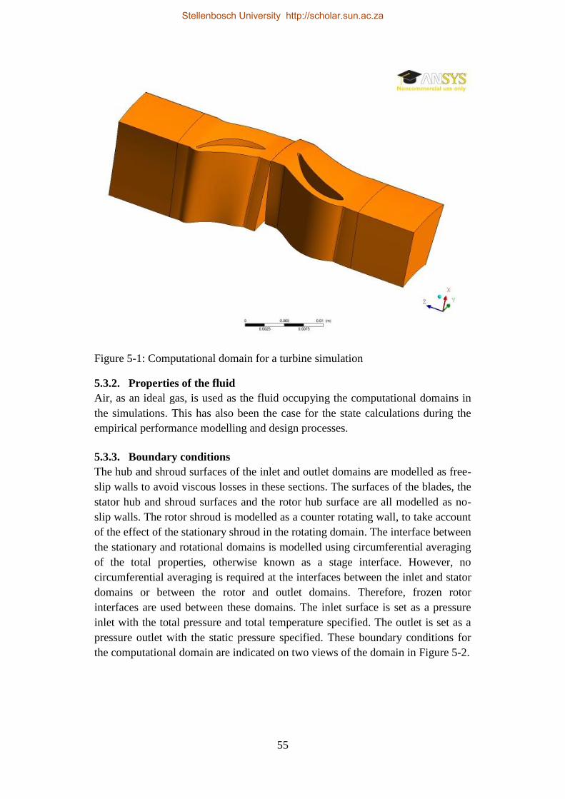
55

Figure 5-1: Computational domain for a turbine simulation

5.3.2. Properties of the fluid

Air, as an ideal gas, is used as the fluid occupying the computational domains in

the simulations. This has also been the case for the state calculations during the

empirical performance modelling and design processes.

5.3.3. Boundary conditions

The hub and shroud surfaces of the inlet and outlet domains are modelled as free-

slip walls to avoid viscous losses in these sections. The surfaces of the blades, the

stator hub and shroud surfaces and the rotor hub surface are all modelled as no-

slip walls. The rotor shroud is modelled as a counter rotating wall, to take account

of the effect of the stationary shroud in the rotating domain. The interface between

the stationary and rotational domains is modelled using circumferential averaging

of the total properties, otherwise known as a stage interface. However, no

circumferential averaging is required at the interfaces between the inlet and stator

domains or between the rotor and outlet domains. Therefore, frozen rotor

interfaces are used between these domains. The inlet surface is set as a pressure

inlet with the total pressure and total temperature specified. The outlet is set as a

pressure outlet with the static pressure specified. These boundary conditions for

the computational domain are indicated on two views of the domain in Figure 5-2.


56

Figure 5-2: CFD boundary conditions

5.3.4. Spatial discretisation

ANSYS CFX Turbogrid is used to discretise the different computational domains

into cells. The built-in optimised Automatic Topology and Meshing (ATM

optimised) feature creates a structured hexahedral cell mesh that follows the

geometry of the blade surfaces and is aligned with the flow direction. For each

blade model the design blade Reynolds number is used to ensure acceptable wall

y+ values. The blade Reynolds number for each design is obtained from the

results of the empirical performance analysis at the design point. The target

number of elements in the mesh is also set. The mesh independence of the flow

solutions is checked and the particulars of the mesh independence study are

shown in Appendix C.2. Figure 5-3 shows the mesh generated for the 105% work

coefficient design stator and inlet domains. The structured nature of the mesh is

clearly visible.

r

z

z

θ

periodic

periodic

periodic

periodic

wall

wallfrozen rotor

interface

frozen rotor

interface

circumferentially

averaging

interface

wall wall free slip

wall

free slip

wall

free slip

wall

free slip

wall

counter

rotating

wallwall

static

pressure

outlet

total

pressure

inlet

Inlet

domain

Stator

domain

Rotor

domain

Outlet

domain


57

Figure 5-3: Computational mesh of the stator and inlet domains

5.3.5. Solver control parameters

The flow being modelled is steady, three-dimensional, compressible, adiabatic

and turbulent. It is modelled using the ANSYS CFX turbomachinery simulation

tool and solved using the ANSYS CFX solver manager. The turbulence is

modelled using the k-ω shear stress transport turbulence model, since it is widely

used for turbomachinery (Djouimaa, et al., 2007). The CFX high resolution

scheme, a second order interpolation scheme, is used to interpolate the advection

of flow properties. This is the scheme recommended by the turbomachinery

simulation tool.

Convergence is controlled by firstly ensuring mesh and domain size independence

as detailed in Appendix C.2. Secondly target root mean square residual values for

the mass, momentum and energy conservations equations and turbulence transport

equations are set to 10-10.

5.4. CFD performance analysis

5.4.1. Analysis procedure

The goal of performing a CFD performance analysis on a prospective turbine

design is to generate points on a turbine performance map. These points can then

be compared to the corresponding curve generated by the empirical model

performance analysis.


58

The empirical model performance analysis of Section 3 predicts the performance

of a turbine design by solving the one-dimensional mean radius flow in a turbine

stage for a range of total-to-static pressure ratios. The total-to-static pressure ratio

is varied by keeping the inlet total pressure and total temperature constant and

altering the outlet static pressure. The results of such an analysis are used to create

curves of mass flow and total-to-total efficiency against total-to-total pressure

ratio for a given turbine design.

The CFD performance analysis simulates the full three-dimensional flow in a

turbine stage for a given set of inlet total conditions and outlet static pressure. As

with the empirical performance analysis, the inlet total conditions are kept

constant across multiple flow field solutions, whilst the outlet static pressure is

varied between solutions. This procedure can also be used to produce performance

curves similar to those generated during the empirical performance analysis.

However, the solutions to full three-dimensional flow simulations take much

longer to obtain than one-dimensional mean radius flow solutions. Therefore, the

three-dimensional flow field is solved for only three simulations for each turbine

design. These three simulations of each turbine design are labelled A, B and C;

and each have a different outlet static pressure. The solution to each of these three

simulations corresponds to a point on the performance maps of that specific

turbine design. These points can then be compared to the curve generated by the

empirical performance analysis.

A CFD performance analysis is conducted on the existing turbine design and the

three new designs. The same values for the inlet total pressure and total

temperature are used for all three simulations of all four designs. These values

correspond to the design parameters identified in Table 4-3. Since the results of

the analysis are to be plotted against total-to-total pressure ratio, similar values of

this parameter are chosen for the simulations of each design. The results of the

empirical performance analysis conducted in Section 4 are used to choose the

outlet static pressures that result in approximate total-to-total pressure ratios of

1.4, 1.6 and 1.8 respectively. The inlet and outlet conditions for each simulation

are shown in Table 5-1 on the next page.

5.4.2. CFD analysis results and discussion

The results of the CFD performance analysis of the BMT 120 KS turbine are used

to create points on the turbine performance map in Figure 5-4 on the next page.

The CFD results are shown as square markers against the curves resulting from

the corresponding performance analysis using the empirical model (EM). The

CFD analysis predicts both higher efficiencies and mass flow rates across the

range of pressure ratios simulated than the empirical performance analysis.


59

Table 5-1: CFD performance analysis inlet and outlet conditions

Inlet total temperature, 𝑇𝑡0 1119 K

Inlet total pressure, 𝑝𝑡0 308 kPa

Outlet static pressure, 𝑝3

Turbine design Simulation A Simulation B Simulation C

BMT 120 KS turbine 208 kPa 177 kPa 149 kPa

95 % work coefficient 204 kPa 174 kPa 146 kPa



Figure 5-4: BMT 102 KS turbine

The results of the CFD performance analysis of the 95 % work coefficient turbine

design are shown in Figure 5-5 on the next page. There is much better agreement

between the results of the two analyses for this new design than for the BMT 120

KS turbine. The CFD performance analysis predicts very similar total-to-total

stage efficiencies to those predicted by the empirical performance analysis.

-1.2

-1

-0.8

-0.6

-0.4

-0.2

0

0.2

0.4

0.6

0.8

1

0

0.2

0.4

0.6

0.8

1

1.2

1.4

1.6

1.8

2

2.2

1 1.2 1.4 1.6 1.8 2

Turb

ine

tota

l-to

-tota

l ise

ntr

opic

ef

fici

ency

, ηtt

Dim

ensi

onle

ss m

ass

flow

rat

e,

m/m

des

ign

Stage total-to-total pressure ratio, pt0/pt3

Mas flow rate - EMMass flow rate - CFDEfficiency - EMEfficiency - CFD


60

However, slightly lower mass flow rates are predicted at higher total-to-total

pressure ratios by the CFD analysis than the empirical performance analysis.

Figure 5-5: 95 % work coefficient design

Figure 5-6 on the next page shows the results of the CFD performance analysis of

the 100 % work coefficient turbine design. The results of the two analyses

correspond equally well to those of the 95 % work coefficient design. The CFD

analysis of the 100 % work coefficient design also predicts lower mass flow rates

at higher total-to-total pressure ratios than the corresponding empirical

performance analysis.

Figure 5-7 on the next page provides a comparison of the results of the CFD and

empirical performance analyses of the 105 % work coefficient turbine design. As

with the other new designs, the results of the two analyses correspond better than

for the BMT 120 KS turbine. In addition, like for the other new designs, the mass

flow and the total-to-total efficiencies predicted by the CFD simulations are lower

than those predicted by the empirical performance.

A general trend in the comparisons of the CFD and empirical model results for the

different turbine designs can be observed. The CFD and empirical performance

analyses predict quite similar results for the new turbine designs. However, the

two analyses predict substantially different mass flow rates and total-to-total

efficiencies for the BMT 120 KS turbine. Nevertheless, the CFD performance

-1.2

-1

-0.8

-0.6

-0.4

-0.2

0

0.2

0.4

0.6

0.8

1

0

0.2

0.4

0.6

0.8

1

1.2

1.4

1.6

1.8

2

2.2

1 1.2 1.4 1.6 1.8 2

Turb

ine

tota

l-to

-tota

l ise

ntr

opic

ef

fici

ency

, ηtt

Dim

ensi

onle

ss m

ass

flow

rat

e,

m/m

des

ign




61



analysis results of the BMT 120 KS turbine are very similar to those of the new

designs. Such similarity in performance is expected, since the new designs are

designed to work at either identical or very similar operating conditions to the

existing turbine design. Therefore, since the convergence of the various CFD

-1.2

-1

-0.8

-0.6

-0.4

-0.2

0

0.2

0.4

0.6

0.8

1

0

0.2

0.4

0.6

0.8

1

1.2

1.4

1.6

1.8

2

2.2

1 1.2 1.4 1.6 1.8 2

Turb

ine

tota

l-to

-tota

l ise

ntr

opic

ef

fici

ency

, ηtt

Dim

ensi

onle

ss m

ass

flow

rat

e,

m/m

des

ign



-1.2

-1

-0.8

-0.6

-0.4

-0.2

0

0.2

0.4

0.6

0.8

1

0

0.2

0.4

0.6

0.8

1

1.2

1.4

1.6

1.8

2

2.2

1 1.2 1.4 1.6 1.8 2

Turb

ine

tota

l-to

-tota

l ise

ntr

opic

ef

fici

ency

, ηtt

Dim

ensi

onle

ss m

ass

flow

rat

e,

m/m

des

ign




62

simulations has also been established with some confidence, the CFD analysis is

concluded to yield the more authoritative performance results. Conversely, it is

then also concluded that the empirical performance analysis does not accurately

predict the performance of the BMT 120 KS turbine. The empirical performance

analysis procedure, however, appears to predict the performance of the new

designs with more accuracy.

The empirical performance analysis procedure uses a free-vortex flow field

assumption. The new turbine designs were designed to produce such a free-vortex

flow field, but the BMT 120 KS turbine was not. Therefore, the difference in

performance prediction accuracy suggests that the use of the empirical

performance analysis procedure is limited to turbine designs with free-vortex

blading.

5.5. Conclusion

CFD performance analyses of the existing BMT 120 KS turbine and three new

turbine designs are described. The CFD methodology is explained and the

performance analysis procedure is described. The results of the CFD performance

analysis are compared to the corresponding empirical performance analysis results

for each turbine design. It is found that the two analyses yield very similar results

for the new turbine designs. However, significant discrepancies between the

performance results of the two analyses are found for the BMT 120 KS turbine.

Since the results of the CFD performance analyses of both the existing turbine and

the new designs yield the expected values, the CFD analysis procedure is

concluded to be more accurate. It is also concluded that the performance analysis

procedure based on empirical data only yields accurate results for turbines

designed to produce free-vortex flow fields.


63

6. FEM structural analysis of turbine rotor

6.1. Introduction

A finite element method (FEM) analysis is performed on the BMT 120 KS turbine

rotor and the rotors of the 95 %, 100 % and 105 % turbine designs. The purpose

of the FEM structural analysis of a rotor is to determine whether it would survive

the mechanical and thermal loads experienced during turbine operation.

The physical conditions to be simulated during the FEM analyses are described,

along with the finite element model. A static structural analysis is conducted and a

conclusion is made on the structural integrity of each rotor design. Furthermore, a

modal analysis of each design is conducted. This allows the reaction of each

design to cyclic excitations during operation to be evaluated.

6.2. Physical conditions simulated

The high temperature gas flow field within the turbine stage induces a static

pressures difference across the rotor blade surface. The resulting torque acts to

drive the rotating engine components at a constant rotational speed. The turbine

blades are therefore subjected to a bending moment due to the aerodynamic

surface loading. The entire turbine rotor disc is also subject to stresses caused by

the centrifugal force generated by its rotational speed. The turbine rotor disc also

experiences thermal loading due to the high temperatures of the gas in the

surrounding flow field. These three loading effects cause significant stresses

within the turbine rotor disc and displacement of the rotor blade tips.

6.3. FE modelling of the physical problem

6.3.1. Geometry of the structural model

The influence of the operating conditions of a turbine can be simulated by

creating a structural model of the entire turbine rotor disc. The effects of the loads

experienced during operation would then be calculated for the entire turbine rotor

disc structural model. However, such a structural model of the full rotor disc

would consist of a number of identical sectors equal to the number of blades. Each

of these sectors would experience identical loading and, therefore, identical

stresses and displacements. Therefore, with the addition of the appropriate

structural constraints, only one sector has to be modelled. The resulting reduction

in structural model size would result in a less computationally intensive analysis.

The geometry of the turbine rotor sector can be seen in Figure 6-1.


64

6.3.2. Material properties

The material properties given to the structural model are those of Inconel IN 713

LC, the material used in the BMT 120 KS turbine. The material properties

relevant to the structural analysis are the density, the modulus of elasticity, the

Poisson’s ratio, the thermal expansion coefficient and the yield strength. These

properties are shown in Table D-1 in Appendix D.

6.3.3. Structural constraints

The turbine rotor sector model is supported by frictionless surface supports on the

two sliced surfaces. These supports constrain the blade sector circumferentially,

but allow free movement in the radial direction. This configuration accurately

simulates the supporting effect that the adjacent blade sectors would have in a full

geometrical model simulation. To constrain any axial rigid body motion, a

frictionless support is also applied to the forward-most hub surface. One of the

circumferential constraints and the axial constraint can be seen in Figure 6-1 as

blue surfaces.

Figure 6-1: FEM model structural constraints


65

6.3.4. Structural loads

The turbine rotor is subjected to centrifugal, thermal and pressure loads during

operation. The centrifugal load is modelled as an inertial load caused by the

rotational velocity. The thermal load is modelled as constant temperature increase

across the entire model. The average turbine inlet temperature at the design point

as calculated by the CFD analysis is used to determine the magnitude of the

temperature increase. This increase in temperature causes thermal expansion of

the structural model and also influences some of the material mechanical

properties. The force caused by the difference in aerodynamic pressure across the

blade is modelled as a circumferential force acting on the blade tip. The

magnitude of the force is specified to result in an equivalent torque to that

obtained from the CFD analysis. In reality, the aerodynamic load is distributed

across the length of the blade. However, applying an equivalent load at the tip of

the blade results in higher bending moments at the root of the blade. Therefore,

this simplification is deemed to be conservative. The circumferential tip force is

shown as an arrow in Figure 6-1.

6.3.5. Structural model discretisation

The geometry of the rotor model is divided into elements using the ANSYS

Workbench mechanical meshing tool. The predominantly hexahedral elements are

sized to be smaller on the blade than on the hub. A mesh independence study is

done to verify the mesh independence of both the static structural and the modal

solutions. These studies are shown in Appendix D. The computational mesh of the

95 % work coefficient turbine design structural model is shown in Figure 6-2. The

illustrated mesh has approximately 45,000 elements.


66

Figure 6-2: Computational mesh of the 95 % work coefficient turbine design

model

6.4. Static structural analysis

The purpose of the static structural analysis of the turbine rotor model is to

determine whether the displacement of the blade tip and the blade root stresses are

within allowable limits. The rotational velocity is set to match the design

rotational speed of 120,000 revolutions per minute, the temperature increase is set

to 707 °C and the circumferential tip force is set to 5 N. The resulting maximum

tip deflections and Von-Mises blade root stresses for each design are shown in

Table 6-1.

At the approximate turbine inlet temperature of 980 K the yield strength is found

by linear interpolation to be 772 MPa. The simulated maximum Von-Mises blade

root stresses of all the turbine designs are comfortably below this yield stress.

Therefore, all the designs are deemed to satisfy the static structural strength

requirements.

Table 6-1: Static structural analysis results

Turbine design Maximum total tip

deflection, mm

Maximum Von-Mises

root stress, MPa

MBT 120 KS turbine 0.394 675


67

95 % work coefficient 0.393 702



6.5. Modal analysis

Excessive structural vibrations induced by unsteady wake flow are a major

concern for axial-flow turbine designers (Lau, et al., 2007). This modal analysis of

the turbine rotor determines whether any of the dominant excitation frequencies

approach any of the turbine rotor natural frequencies as the engine is spun up to

its design speed of 120,000 revolutions per minute. This analysis is conducted at

the same temperature as the static structural analysis. The dominant excitation

frequencies considered in the analysis are the stator blade passing frequencies

encountered in one rotation and the rotational frequency. The 95 %, 100 % and

105 % turbine designs all have a prime number of stator blades. These stator blade

counts are seventeen, seventeen and nineteen respectively. Therefore, only one

stator passing frequency is encountered during one rotation. However, the BMT

120 KS has fifteen stator blades and therefore three passing frequencies are

encountered in one rotation. The two additional frequencies are excited by every

third and every fifth stator blade.

The results of the modal analyses are used to construct Campbell diagrams of the

four turbine rotor designs. The results of the modal analysis of the BMT 120 KS

turbine rotor are shown in Figure 6-3. The natural frequencies of the first six

vibration modes are shown as markers and the dominant stator blade passing

frequencies are shown as solid and dotted lines. It can be seen that the passing

frequency of every third and fifth stator blade are very close to respectively the

first and second natural frequencies at the design speed.


68

Figure 6-3: Campbell diagram of the BMT 120 KS turbine rotor

Figure 6-4 and Figure 6-5 on the next two pages show the Campbell diagrams for

the 95 % and 100 % work coefficient designs respectively. The modal analysis

results of these two designs are quite similar. The stator blade passing frequencies

are comfortably far from all the turbine rotor blade natural frequencies at the

design speed of 120,000 revolutions per minute.

0

10

20

30

40

50

60

0 20 40 60 80 100 120

Fre

qu

ency

, k

Hz

Turbine rotational speed, n, krpm

mode 1

mode 2

mode 3

mode 4

mode 5

mode 6

15n excitation

5n excitation

3n excitation

n excitation


69

Figure 6-4: Campbell diagram of the 95 % work coefficient turbine rotor


The Campbell diagram for the 105 % work coefficient design is shown in Figure

6-6. The natural frequencies of this rotor design are very similar to those of the

other two new designs. However, the larger stator blade count causes the stator

blade passing frequency to be slightly higher. This increase brings the stator blade

0

10

20

30

40

50

60

0 20 40 60 80 100 120

Fre

qu

ency

, k

Hz


mode 1

mode 2

mode 3

mode 4

mode 5

mode 6

17n excitation

n excitation

0

10

20

30

40

50

60

0 20 40 60 80 100 120

Fre

qu

ency

, k

Hz


mode 1

mode 2

mode 3

mode 4

mode 5

mode 6

17n excitation

n excitation


70

passing frequency close to the natural frequency of the fourth mode at the design

speed. This might cause structural resonance, resulting in higher than normal

displacements during operation at the design speed.


6.6. Conclusion

The static structural and modal analyses of the BMT 120 KS turbine rotor and the

rotors of the three new designs are described. The FEM methodology is detailed

and the analysis methods are described. It is found that none of the rotors

experience excessively high root stresses during static loading. The results of the

modal analysis, however, suggest that both the BMT 120 KS turbine rotor and the

rotor of the 105 % work coefficient design would encounter structural resonance

when operating at or near the design speed. However, since only the fourth most

prominent natural frequency of the 105 % work coefficient design is excited, the

resulting displacements would likely not be unacceptably high.

0

10

20

30

40

50

60

0 20 40 60 80 100 120

Fre

qu

ency

, k

Hz


mode 1

mode 2

mode 3

mode 4

mode 5

mode 6

19n excitation

n excitation


71

7. Turbine prototype manufacturing process

7.1. Introduction

New turbine designs were generated using the turbine design procedure and

analysed using numerical and empirical procedures. Prototypes of these new

designs are required for use in experimental testing. An investment casting

process is utilised for manufacturing these prototypes. This process is chosen

because it allows each turbine component to be created as a single casting that is

close to the desired final shape. Additionally, when using an investment casting

process, the geometries of the turbine blades are not limited by the machinability

of the material or constricted by tooling access.

This section describes the process followed to create the prototypes of the turbine

components. Firstly, the appropriate material for the prototypes is selected and

three-dimensional models of the desired final geometries are generated. The final

geometries are then modified for the casting process by taking account of

shrinkage and by adding machining allowances. These modified component

geometries are used to create the sacrificial patterns and the investment casting

process is performed. The results of the investment casting process are discussed

and some concluding remarks are made.

7.2. Material selection

The high operating temperatures and mechanical stresses encountered in turbine

blades necessitate the use of high temperature super-alloys. The BMT 120 KS

turbine is manufactured from Inconel IN713LC, a nickel-based super-alloy. As is

shown in Table D-1 in Appendix D.1, the yield strength and modulus of elasticity

of IN713LC are sufficiently high at the temperatures encountered in the turbine

stage. IN713LC also has the added benefit of not requiring heat treatment after the

casting process. Therefore, IN713LC is selected to be the material for the new

turbine.

7.3. Required final component geometries

The prototypes of the new turbine rotor and stator components are to be used in an

un-modified BMT 120 KS jet engine. Therefore, the mounting surfaces of the new

components must be identical to those on the existing BMT 120 KS turbine

components. The turbine rotor hub has a central hole that slips over the jet engine

shaft. It is secured to the shaft by a nut tightened against the back of the hub to

press an extended front shoulder against the shaft bearing. The turbine stator is

attached to the tunnel of the engine by six machine screws through holes in a


72

flange. The axial position of both the stator flange and the rotor hub shoulder

relative to the leading edge of the stator blades also correspond to the distances in

the BMT 120 KS turbine. The outer surface of the stator shroud is also shaped to

fit inside the combustion chamber exhaust at the front and the engine housing at

the back.

7.4. Modification of desired final component geometries

The required final component geometries are modified for the manufacturing

process. These modifications are used to provide machining allowances and

facilitate the flow of the molten nickel alloy through the mould during the

investment casting process. Due to the shrinkages of solidifying metal, a casting is

smaller than its associated wax pattern (Dong, et al., 2011). Therefore, the

modified geometries are scaled up volumetrically by 1.5 % to take account of the

shrinkage of the molten nickel alloy upon solidification. Figure 7-1 shows the

desired stator geometry (left) and the modified stator geometry (right). The

volumetric size increase can’t be clearly seen on this scale, but the machining

allowance added to the outer surface of the shroud can be seen. In the modified

model, the flange is extended to the centre, where it connects to a shoulder. This

shoulder is used for the connection of the component patterns to the casting risers.

Figure 7-1: Stator final (left) and casting (right) geometries


73

7.5. Pattern creation

Three-dimensional printers are used to grow the investment casting patterns one

layer of material at a time. Two different printing systems, each characterised by

the use of a distinct material, are used for growing the patterns. The one system

employs an EOSINT P380 that grows three-dimensional geometries by laser-

sintering powdered layers of PrimeCast 101, a polystyrene material. The other

system uses a Solidscape 3Z Pro printer to grow parts by expelling a jet of micro

droplets of a Solidscape 3Z Model, a wax-like organic compound.

7.5.1. PrimeCast 101 system

The EOSINT P380 creates three-dimensional models by selectively laser-sintering

multiple layers of PrimeCast 101 powder. The powder is low cost, with the bulk

of the production cost being related to the production duration. Therefore, since

the EOSINT P380 has the capacity to grow multiple parts simultaneously, the

patterns of multiple different turbine designs could be grown inexpensively.

An example of a turbine rotor pattern generated using the PrimeCast 101 system

is shown in Figure 7-2. The part can be seen to have a rough surface finish, with a

significant stepping effect on the hub surface being visible. Furthermore, the

feature creation resolution appears to be coarse, as is visible on the blade jagged

trailing edges. The PrimeCast 101 model is also fairly brittle, resulting in the

chipping of the blade tips during transportation.

Figure 7-2: PrimeCast 101 rotor pattern


74

7.5.2. Solidscape 3Z Model system

The Solidscape 3Z Pro creates three-dimensional models by expelling a high

frequency jet of Solidscape 3Z Model micro droplets. The jet is precision

controlled and can be used to reproduce intricate geometries and smooth surfaces.

The Solidscape 3Z Model material is more expensive than the PrimeCast 101

material and the Solidscape 3Z Pro has the capacity to grown only one part at a

time. Due to these two factors, a Solidscape 3Z Model part is about seventy times

more expensive to produce than an equivalent PrimeCast 101 part.

An example of a turbine rotor pattern generated using the Solidscape 3Z Model

system is shown in Figure 7-3. The part can be seen to have a much smoother

surface finish than the comparable PrimeCast 101 pattern, with a no visible

stepping effect on the smooth surfaces. The printing resolution is also suitably

high for accurately producing the thin blade trailing edges.

Figure 7-3: Solidscape 3Z Model rotor pattern

7.6. Investment casting process

The sacrificial component patterns are assembled using sections of wax rod.

These assemblies are then repeatedly dipped in ceramic slurry and dried, thus

building a substantial ceramic shell. The patterns with the encasing ceramic shell

are then placed in an oven where the patterns are burned out, thus leaving only the

ceramic shell mould.


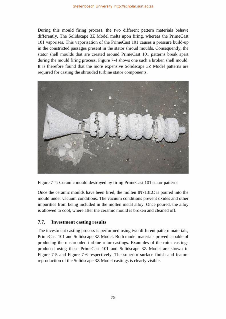
75

During this mould firing process, the two different pattern materials behave

differently. The Solidscape 3Z Model melts upon firing, whereas the PrimeCast

101 vaporises. This vaporisation of the PrimeCast 101 causes a pressure build-up

in the constricted passages present in the stator shroud moulds. Consequently, the

stator shell moulds that are created around PrimeCast 101 patterns break apart

during the mould firing process. Figure 7-4 shows one such a broken shell mould.

It is therefore found that the more expensive Solidscape 3Z Model patterns are

required for casting the shrouded turbine stator components.

Figure 7-4: Ceramic mould destroyed by firing PrimeCast 101 stator patterns

Once the ceramic moulds have been fired, the molten IN713LC is poured into the

mould under vacuum conditions. The vacuum conditions prevent oxides and other

impurities from being included in the molten metal alloy. Once poured, the alloy

is allowed to cool, where after the ceramic mould is broken and cleaned off.

7.7. Investment casting results

The investment casting process is performed using two different pattern materials,

PrimeCast 101 and Solidscape 3Z Model. Both model materials proved capable of

producing the unshrouded turbine rotor castings. Examples of the rotor castings

produced using these PrimeCast 101 and Solidscape 3Z Model are shown in

Figure 7-5 and Figure 7-6 respectively. The superior surface finish and feature

reproduction of the Solidscape 3Z Model castings is clearly visible.


76

Figure 7-5: Rotor casting made using a PrimeCast 101 pattern

Figure 7-6: Rotor casting made using a Solidscape 3Z Model pattern

Only the Solidscape 3Z Model patterns resulted in usable shrouded stator moulds.

An example of a turbine stator, cast using a Solidscape 3Z Model pattern, is

shown in Figure 7-7. The surface finish and feature reproduction are similar to

those of the turbine rotor castings that used the same pattern material.


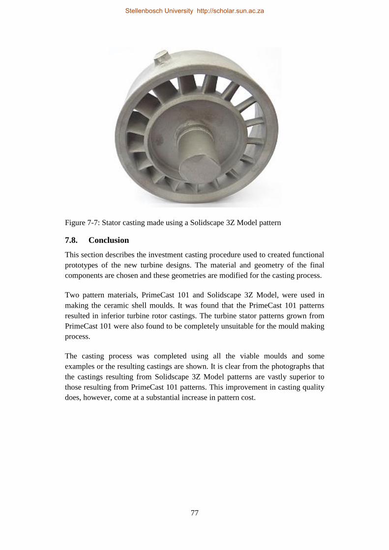
77

Figure 7-7: Stator casting made using a Solidscape 3Z Model pattern

7.8. Conclusion

This section describes the investment casting procedure used to created functional

prototypes of the new turbine designs. The material and geometry of the final

components are chosen and these geometries are modified for the casting process.

Two pattern materials, PrimeCast 101 and Solidscape 3Z Model, were used in

making the ceramic shell moulds. It was found that the PrimeCast 101 patterns

resulted in inferior turbine rotor castings. The turbine stator patterns grown from

PrimeCast 101 were also found to be completely unsuitable for the mould making

process.

The casting process was completed using all the viable moulds and some

examples or the resulting castings are shown. It is clear from the photographs that

the castings resulting from Solidscape 3Z Model patterns are vastly superior to

those resulting from PrimeCast 101 patterns. This improvement in casting quality

does, however, come at a substantial increase in pattern cost.


78

8. Conclusion

The purpose of this thesis is to document the proposed methodology for designing

axial-flow turbines for use in small jet engines. The resulting methodology would

complement similar research done on the development of centrifugal compressors.

8.1. Development and implementation of the design methodology

At the outset of this project the design methodology was divided up into six

sections, each meant to address one of the project objectives. The following

paragraphs present a summary of the methods used and the results obtained in

each section. Reference is also made to how each section addresses a particular

project objective.

In Section 2 the geometries of existing turbine components are reverse engineered

to allow for a comparative analysis with new turbine designs. The shapes of the

turbine stator and rotor are digitised using a CT-scanner and a CMM respectively.

The procedure for processing the raw point cloud data obtained from the two

measurement devices is described and renderings of the resulting reconstructed

three-dimensional models are shown. These three-dimensional models can be

used in a CFD analysis of the existing turbine and can also be readily

parameterised for use in an empirical performance analysis procedure. The

models of the existing turbine can therefore be used as a baseline design and serve

to meet the first project objective.

Section 3 details a mean radius performance analysis procedure using empirical

loss correlations. The empirical loss model is described and a proposal for an

analysis procedure for calculating the performance of a turbine under specified

conditions is made. This procedure is applied to an existing turbine design and a

turbine performance map is generated. This performance map compares well with

the trends shown in similar charts in literature, even though the mass flow rate is

under predicted. This empirical loss model performance analysis procedure serves

as one of independent performance analysis procedures required to partially meet

the third project objective.

In Section 4 the design process of a replacement turbine for an existing micro jet

engine is described. The process for obtaining the design parameters is shown and

a method for designing a turbine to meet those design parameters is presented.

The method is used to generate three candidate designs, which are then subjected

to the empirical performance analysis detailed in Section 3. The results of the

analysis are encouraging, suggesting suitably high efficiencies and mass flow

rates for the new designs. Therefore, further analysis of the new designs is


79

deemed justified. Since this design process is shown to be able to generate viable

turbine designs, the second project objective is deemed to be met.

CFD performance analyses of the existing BMT 120 KS turbine and three new

turbine designs are described in Section 5. The CFD methodology is detailed and

the performance analysis procedure is described. The results of the CFD

performance analysis are compared to the corresponding empirical performance

analysis results for each turbine design. It is found that the two analyses yield very

similar results for the new turbine designs. However, significant discrepancies

between the performance results of the two analyses are found for the BMT 120

KS turbine. Since the results of the CFD performance analyses of both the

existing turbine and the new designs yield the expected values, the CFD analysis

procedure is concluded to be more accurate. This CFD performance analysis

procedure serves as a second independent procedure, and therefore the third

objective is fully met.

The static structural and modal analyses of the BMT 120 KS turbine rotor and the

rotors of the three new designs are described in Section 6. The FEM methodology

is detailed and the analysis methods are described. It is found that none of the

rotors experience excessively high root stresses during static loading. The results

of the modal analysis suggest that the BMT 120 KS turbine rotor and the rotor of

the 105 % work coefficient design would have natural frequencies excited at or

near the design speed. These are, however, not the primary natural frequencies, so

excessive blade deflections are not expected. This structural analysis procedure

serves to meet the fourth project objective.

Section 7 describes the investment casting procedure used to create functional

prototypes of the new turbine designs. IN 713 LC is chosen as the material for the

prototypes, and the geometries of the different components are modified to make

provisions for the casting process. Two pattern materials, PrimeCast 101 and

Solidscape 3Z Model, are used in making the ceramic shell moulds. It was found

that the PrimeCast 101 patterns result in inferior turbine rotor castings. The

turbine stator patterns grown from PrimeCast 101 are also found to be unsuitable

for the mould making process. The casting process is completed using all the

viable moulds and some examples or the resulting castings are shown. It is clear

from the photographs that the castings resulting from Solidscape 3Z Model

patterns feature substantially better surface finish and thin edge reproduction

compared to those resulting from PrimeCast 101 patterns. Future experimental

analysis of the different castings may indicate whether the additional cost of using

Solidscape 3Z Model patterns is justified. Since this manufacturing process


80

successfully produced turbine prototype castings, the fifth project objective is

deemed as met.

8.2. Suggestions for future research

The present project focussed on the design process as a whole. Consequently, in

depth studies of each of the design steps were not possible. Therefore, there is an

opportunity for research into each of the design steps individually. A CFD

investigation into the effect of different turbine stage work coefficients on the

flow field would be especially helpful.

Since this project excluded the final machining of the cast turbine prototypes, and

also the experimental testing of the new designs, these tasks remain as scope for a

future project. An experimental investigation into the difference in the

performance of turbine castings made using PrimeCast 101 patterns and castings

made using Solidscape 3Z Model patterns would also shed light on the necessity

of using expensive pattern materials.

When the results of the present project are seen in the context of the greater

Ballast project, an important perspective is gained. Clearly an opportunity exists

for developing a new turbine and a new centrifugal compressor to be used

together in a micro jet engine.


81

Appendix A: Empirical performance model calculations

A.1. BMT 120 KS turbine stator blade row total pressure loss

coefficient sample calculation

The total pressure loss coefficient of the BMT 120 KS turbine stator blade row is

dependent on the parameters listed in Table A-1 and is calculated using equation

(3.2) (Aungier, 2006):

𝑌 = 𝑌𝑇𝐸 + 𝑌𝑝 + 𝑌𝑠 + 𝑌𝐶𝐿 + 𝑌𝑆𝐻 = 0,131 (A-1)

Table A-1: BMT 120 KS turbine stator blade row empirical performance model

inlet parameters

The calculations for the different loss coefficients in equation (A-1) are now

shown.

A.1.1. Trailing edge loss coefficient calculation

The trailing edge loss coefficient is calculated using equation (3.3):

A.1.2. Profile loss coefficient calculation

The profile loss coefficient is calculated using equation (3.4) (Aungier, 2006):

𝑌𝑝 = 𝐾𝑚𝑜𝑑 𝐾𝑖𝑛𝑐 𝐾𝑀 𝐾𝑝 𝐾𝑅𝐸 ((𝑌𝑝1 + 𝜉2(𝑌𝑝2 − 𝑌𝑝1)) (5𝑡𝑚𝑎𝑥

𝑐)

𝜉

− 𝛥𝑌𝑇𝐸)

= 0,0246

(A-3)

Blade parameters Flow field parameters

𝛽𝑏0 96,81° 𝛼𝑏0′ 90°

𝛽𝑔 28,34° 𝛼𝑏1′ 32,1°

𝑏𝑧 10,8 mm 𝑊1 321 m/s

𝑐 14,0 mm 𝑀0′ 0,23

𝑠 11,6 mm 𝑀1′ 0,49

𝑠/𝑐 0,825 𝜌1 0,833 kg/m3

𝑅𝑐 33,1 mm 𝜇1 4,4(10)-5 kg/m/s

𝑡𝑚𝑎𝑥 2 mm

𝑡𝑇𝐸 0,9 mm

𝑒 0,05 mm

ℎ 10,1 mm

𝛿 0 mm

𝑌𝑇𝐸 = (𝑡𝑇𝐸

𝑠 sin𝛽𝑔 − 𝑡𝑇𝐸)

2

= 0,0376 (A-2)


82

The calculation of the different factors and terms used in equation (A-3) are now

shown.

Nozzle blade and impulse blade profile loss coefficient calculation

The gas deflection ratio is calculated using equation (3.5):

𝜉 =90° − 𝛽𝑏0

90° − 𝛼𝑏1′ = −0,118 (A-4)

The ideal nozzle blade and impulse blade pitch-to-chord ratios are given by

equation (A-5) and equation (A-6) respectively (Aungier, 2006):

(𝑠/𝑐)𝑚𝑖𝑛,1 = 0,427 +𝛼𝑏1

′

58°− (

𝛼𝑏1′

93°)

2

= 0,862 (A-5)

(𝑠/𝑐)𝑚𝑖𝑛,2 = 0,224 + (1,575 −𝛼𝑏1

′

90°)(

𝛼𝑏1′

90°) = 0,659 (A-6)

The nozzle blade and impulse blade profile loss coefficients are given by

equations (A-7) to (A-12) and equation (A-13) to (A-17) respectively (Aungier,

2006):

𝑋𝑝1 = (𝑠/𝑐) − (𝑠/𝑐)𝑚𝑖𝑛1 = −0,0365 (A-7)

𝐴𝑝1 =

{

0,025 +27° − 𝛼𝑏1

′

530°, 𝛼𝑏1

′ ≤ 27°

0,025 +27° − 𝛼𝑏1

′

3085°, 𝛼𝑏1

′ > 27°

= 0,0233 (A-8)

𝐵𝑝1 = 0,1583 −𝛼𝑏1

′

1640°= 0,139 (A-9)

𝐶𝑝1 = 0,08 [(𝛼𝑏1

′

30°)

2

− 1] , 𝛼𝑏1′ ≤ 30° (A-10)

𝑛𝑝1 = 1 +𝛼𝑏1

′

30°, 𝛼𝑏1

′ > 30° = 2,07 (A-11)

𝑌𝑝1 = {𝐴𝑝1 + 𝐵𝑝1 𝑋𝑝1

2 + 𝐶𝑝1 𝑋𝑝13 , 𝛼𝑏1

′ ≤ 30°

𝐴𝑝1 + 𝐵𝑝1|𝑋𝑝1|𝑛𝑝1 , 𝛼𝑏1

′ > 30°= 0,0235 (A-12)

𝑋𝑝2 = (𝑠/𝑐) − (𝑠/𝑐)𝑚𝑖𝑛2 = 0,166 (A-13)

𝐴𝑝2 = 0,242 −𝛼𝑏1

′

151°+ (

𝛼𝑏1′

127°)

2

= 0,0932 (A-14)


83

𝐵𝑝2 =

{

0,3 +(30° − 𝛼𝑏1

′ )

50°, 𝛼𝑏1

′ ≤ 30°

0,3 +(30° − 𝛼𝑏1

′ )

275°, 𝛼𝑏1

′ > 30°

= 0,292 (A-15)

𝐶𝑝2 = 0,88 −𝛼𝑏1

′

42,4°+ (

𝛼𝑏1′

72,8°)

2

= 0,317 (A-16)

𝑌𝑝2 = 𝐴𝑝2 + 𝐵𝑝2 𝑋𝑝22 − 𝐶𝑝2 𝑋𝑝2

3 = 0,0998 (A-17)

Off-design incidence angle correction factor calculation

The incidence angle is calculated using equation (3.7):

𝑖 = 𝛽𝑏0 − 𝛼𝑏0′ = 6.81° (A-18)

The gas deflection ratio dependent part of the stalling incidence angle is

calculated using equation (A-19) to equation (A-24) (Aungier, 2006):

𝑖𝑠0 = 20° − (𝜉 + 1

0,11) ° = 12° (A-19)

𝐴𝑠𝑟 = 𝐴𝑠𝑟(𝛼𝑏1′ ) = 61,8° − (1,6° −

𝛼𝑏1′

165°)𝛼𝑏1

′ = 16,6° (A-20)

𝐵𝑠𝑟 = 𝐵𝑠𝑟(𝛼𝑏1′ ) = 71,9° − 1,69𝛼𝑏1

′ = 17,6° (A-21)

𝐶𝑠𝑟 = 𝐶𝑠𝑟(𝛼𝑏1′ ) = 7,8° − (0.28 −

𝛼𝑏1′

320°)𝛼𝑏1

′ = 2,03° (A-22)

𝐷𝑠𝑟 = 𝐷𝑠𝑟(𝛼𝑏1′ ) = 14,2° − (0,16 +

𝛼𝑏1′

160°)𝛼𝑏1

′ = 2,6° (A-23)

𝑖𝑠𝑟(𝛼𝑏1′ , 𝜉) = {

𝑖𝑠0 + 𝐴𝑠𝑟 − 𝐵𝑠𝑟 𝜉2 + 𝐶𝑠𝑟 𝜉

3 + 𝐷𝑠𝑟 𝜉4, 𝛼𝑏1

′ ≤ 40°

𝑖𝑠0 + |55° − 𝛼𝑏1

′

15°| |𝑖𝑠𝑟(40°, 𝜉) − 𝑖𝑠0|, 𝛼𝑏1

′ > 40°

= 28,4°

(A-24)

The pitch-to-chord ratio stalling incidence angle correction is calculated using

equation (3.9) and (3.10):

𝑋𝑖𝑠 = 𝑠/𝑐 − 0,75 = 0,0752 (A-25)


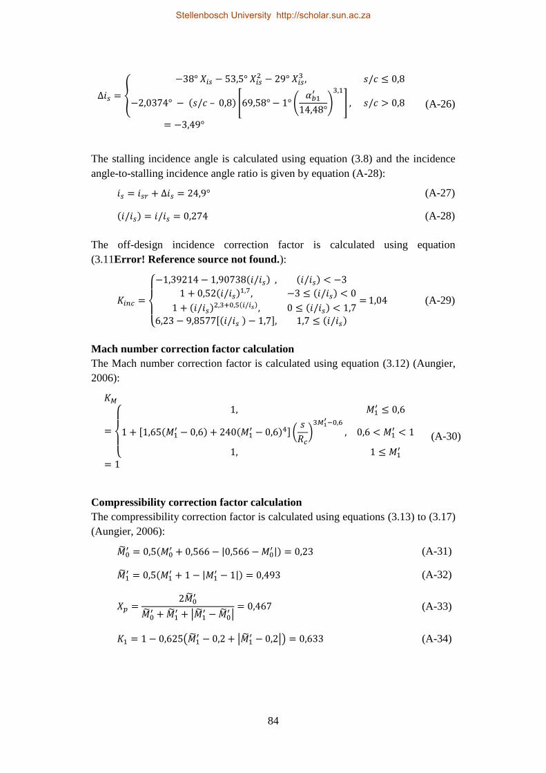
84

∆𝑖𝑠 = {

−38° 𝑋𝑖𝑠 − 53,5° 𝑋𝑖𝑠2 − 29° 𝑋𝑖𝑠

3 , 𝑠/𝑐 ≤ 0,8

−2,0374° − (𝑠/𝑐 – 0,8) [69,58° − 1° (𝛼𝑏1

′

14,48°)

3,1

] , 𝑠/𝑐 > 0,8

= −3,49°

(A-26)

The stalling incidence angle is calculated using equation (3.8) and the incidence

angle-to-stalling incidence angle ratio is given by equation (A-28):

𝑖𝑠 = 𝑖𝑠𝑟 + ∆𝑖𝑠 = 24,9° (A-27)

(𝑖/𝑖𝑠) = 𝑖/𝑖𝑠 = 0,274 (A-28)

The off-design incidence correction factor is calculated using equation

(3.11Error! Reference source not found.):

𝐾𝑖𝑛𝑐 =

{

−1,39214 − 1,90738(𝑖/𝑖𝑠) , (𝑖/𝑖𝑠) < −3

1 + 0,52(𝑖/𝑖𝑠)1,7, −3 ≤ (𝑖/𝑖𝑠) < 0

1 + (𝑖/𝑖𝑠)2,3+0,5(𝑖/𝑖𝑠), 0 ≤ (𝑖/𝑖𝑠) < 1,7

6,23 − 9,8577[(𝑖/𝑖𝑠 ) − 1,7], 1,7 ≤ (𝑖/𝑖𝑠)

= 1,04 (A-29)

Mach number correction factor calculation

The Mach number correction factor is calculated using equation (3.12) (Aungier,

2006):

𝐾𝑀

=

{

1, 𝑀1

′ ≤ 0,6

1 + [1,65(𝑀1′ − 0,6) + 240(𝑀1

′ − 0,6)4] (𝑠

𝑅𝑐)

3𝑀1′−0,6

, 0,6 < 𝑀1′ < 1

1, 1 ≤ 𝑀1′

= 1

(A-30)

Compressibility correction factor calculation

The compressibility correction factor is calculated using equations (3.13) to (3.17)

(Aungier, 2006):

�̃�0′ = 0,5(𝑀0

′ + 0,566 − |0,566 − 𝑀0′ |) = 0,23 (A-31)

�̃�1′ = 0,5(𝑀1

′ + 1 − |𝑀1′ − 1|) = 0,493 (A-32)

𝑋𝑝 =2�̃�0

′

�̃�0′ + �̃�1

′ + |�̃�1′ − �̃�0

′ |= 0,467 (A-33)

𝐾1 = 1 − 0,625(�̃�1′ − 0,2 + |�̃�1

′ − 0,2|) = 0,633 (A-34)


85

𝐾𝑝 = 1 − (1 − 𝐾1)𝑋𝑝2 = 0,92 (A-35)

Reynolds number correction factor calculation

The chord-based, roughness height based, laminar and transition Reynolds

numbers are calculated using equations (A-36) to (A-39) respectively (Aungier,

2006):

The Reynolds number correction factor is then calculated using equation (A-40)

(Aungier, 2006):

𝐾𝑅𝐸 =

{

√𝑅𝑒𝑙𝑎𝑚/𝑅𝑒𝑐 , 𝑅𝑒𝑐 < 𝑅𝑒𝑙𝑎𝑚

1, 𝑅𝑒𝑙𝑎𝑚 < 𝑅𝑒𝑐 < 𝑅𝑒𝑡𝑟

1 + [log(𝑅𝑒𝑡𝑟)

log(𝑅𝑒𝑟)]

2,58

(1 −𝑅𝑒𝑡𝑟

𝑅𝑒𝑐) , 𝑅𝑒𝑟 < 𝑅𝑒𝑡𝑟 < 𝑅𝑒𝑐

[log(𝑅𝑒𝑡𝑟)

log(𝑅𝑒𝑟)]

2,58

, 𝑅𝑒𝑡𝑟 < 𝑅𝑒𝑟 < 𝑅𝑒𝑐

[log(𝑅𝑒𝑡𝑟)

log(𝑅𝑒𝑐)]

2,58

, 𝑅𝑒𝑡𝑟 < 𝑅𝑒𝑐 < 𝑅𝑒𝑟

= 1,083

(A-40)

Trailing edge loss correction factor calculation

The trailing edge loss correction factor is calculated using equation Error!

Reference source not found.) (Aungier, 2006):

∆𝑌𝑇𝐸 = (0,02𝑠

𝑠 sin𝛽𝑔 − 0,02𝑠)

2

= 0,00194 (A-41)

A.1.3. Secondary flow loss coefficient calculation

The secondary flow loss coefficient is calculated using equations (3.20) to (3.26)

(Aungier, 2006):

𝛼𝑚′ = 90° − atan (

cot𝛼𝑏0′ + cot 𝛼𝑏1

′

2)

180°

𝜋= 51,5° (A-42)

𝐶𝐿 = 2|cot 𝛼𝑏1′ − cot𝛼𝑏0

′ | sin 𝛼𝑚′ (𝑠/𝑐) = 2,06 (A-43)

𝑅𝑒𝑐 =𝜌2𝑊2𝑐

𝜇2= 85 300 (A-36) 𝑅𝑒𝑙𝑎𝑚 = 1(10)5 (A-37)

𝑅𝑒𝑟 = 100𝑐

𝑒= 28 000 (A-38) 𝑅𝑒𝑡𝑟 = 5(10)5 (A-39)


86

𝑍 = (𝐶𝐿

(𝑠/𝑐))

2 sin2 𝛼𝑏1′

sin3 𝛼𝑚′ = 3,67 (A-44)

𝐹𝐴𝑅 = {0,5 (2𝑐

𝐻)

0.7

, 𝐻/𝑐 < 2

𝑐/𝐻, 𝐻/𝑐 ≥ 2

= 1,02 (A-45)

�̃�𝑠 = 0,0334𝐹𝐴𝑅𝑍sin𝛼𝑏1

′

sin 𝛽𝑏0= 0,672 (A-46)

𝐾𝑠 = 1 − (1 − 𝐾𝑝) [(𝑏𝑧/𝐻)2

1 + (𝑏𝑧/𝐻)2] = 0,957 (A-47)

𝑌𝑠 = 𝐾𝑅𝐸𝐾𝑠√�̃�𝑠

2

1 + 7,5�̃�𝑠2 = 0,0685 (A-48)

A.1.4. Blade clearance loss coefficient calculation

The blade clearance loss coefficient is calculated using equation (3.27) (Aungier,

2006):

𝑌𝐶𝐿 = 0,47𝑍(𝑐/𝐻)(𝛿/𝑐)0,78 = 0 (A-49)

A.1.5. Shock loss coefficient calculation

The shock loss coefficient is calculated using equations (3.28) to (3.31) (Aungier,

2006):

A.2. Exit static pressure based state solution sample calculations

Interpolations of an ideal gas property table (Cengel & Boles, 2004) are used for

relating the intrinsic thermodynamic properties of air. These linear interpolations

are shown implicitly as one property being a function of another.

𝑋1 = {0, 𝑀0

′ ≤ 0,4

𝑀0′ − 0,4, 𝑀0

′ > 0,4= 0 (A-50)

𝑋2 = {

0, 𝑀0′ <= 𝑀1

′

𝑀0′

𝑀1′ − 1, 𝑀0

′ > 𝑀1′ = 0 (A-51)

�̃�𝑆𝐻 = 0,8𝑋12 + 𝑋2

2 = 0 (A-52)

𝑌𝑆𝐻 = √�̃�𝑆𝐻

2

1 + �̃�𝑆𝐻2 = 0 (A-53)


87

A.2.1. Stator inlet state solution: sample calculation

The values of the known flow field, gas property and geometric parameters at the

stator inlet are shown in Table A-2.

Table A-2: Known parameter values at the stator inlet

Parameter Known value

Cross-sectional flow area, 𝐴0 0,001752 m2

Absolute flow angle, 𝛼0 0°

Total temperature, 𝑇𝑡0 1119 K

Total pressure, 𝑝𝑡0 308,3 kPa

Total temperature dependent specific entropy, 𝑠𝑡0𝑜 3,097 kJ/kg/K

Static pressure, 𝑝0 297,3 kPa

The calculations for obtaining the mass flow rate at the stator inlet are shown in

equations (A-54) to (A-60):

𝑠0𝑜 = 𝑠0𝑡

𝑜 + 𝑅𝑎𝑖𝑟 ln(𝑝0/𝑝𝑡0) = 3,087 kJ/kg/K (A-54)

ℎ0 = ℎ(𝑠00) = 1172 kJ/kg (A-55)

𝑇0 = 𝑇(𝑠0𝑜) = 1109 K (A-56)

𝜌0 = 𝑝0/(𝑅𝑎𝑖𝑟 𝑇0 ) = 0,934 kg/m3 (A-57)

ℎ𝑡0 = ℎ(𝑇𝑡0) = 1183 kJ/kg (A-58)

𝐶0 = √2(ℎ𝑡0 − ℎ0) = 152,3 m/s (A-59)

�̇�0 = 𝐴0𝜌0𝐶0 cos𝛼0 = 0,249 kg/s (A-60)

A.2.2. Stator exit state solution: sample calculation


stator exit are shown in Table A-3.

Table A-3: Known parameter values at the stator exit



Blade angle, 𝛽1 57,86°


88

Total enthalpy, ℎ𝑡1 1183 kJ/kg


The calculations for obtaining the mass flow rate at the stator exit are shown in

equations (A-61) to (A-69). Since only the last iteration is shown, the stator blade

row total pressure loss coefficient has already converged to the value shown in

(A-61):

𝑌𝑆 = 0,125 (A-61)

𝑠𝑡1𝑜 = 𝑠𝑜(ℎ𝑡1) = 3,097 kJ/kg/K (A-62)

𝑠1𝑜 = 𝑠𝑡1

𝑜 − 𝑅𝑎𝑖𝑟 ln (𝑝𝑡0 + 𝑝1𝑌𝑆

𝑝1 + 𝑝1𝑌𝑆) = 3,05 kJ/kg/K (A-63)

𝑇1 = 𝑇(𝑠1𝑜) = 1075 K (A-64)

𝜌1 = 𝑝1/(𝑅𝑎𝑖𝑟 𝑇1 ) = 0,833 kg/m3 (A-65)

ℎ1 = ℎ(𝑇1) = 1132 kJ/kg (A-66)

𝐶1 = √2(ℎ𝑡1 − ℎ1) = 321,1 m/s (A-67)

𝛼1 = 𝛽1 = 57,86° (A-68)

�̇�1 = 𝜌1𝐴1𝐶1 cos(𝛼1) = 0,249 kg/s (A-69)

A.2.3. Rotor inlet state solution: sample calculation


rotor inlet are shown in Table A-4. Furthermore, at the stator exit, the mean radius

is taken to be 27.65 mm and the values for the absolute gas velocity are as in the

previous section.

Table A-4: Known parameter values at the rotor inlet



Total enthalpy, ℎ𝑡2 1183 kJ/kg

Total pressure, 𝑝𝑡2 302,6 kPa

Mean radius, 𝑟𝑚2 27,62 mm

Static density guess, 𝜌2 0,838 kg/m3


89

The axial component of the absolute gas velocity at the rotor inlet is calculated in

equation (A-70) and the circumferential component is calculated using equation

(3.37). The magnitude of the absolute gas velocity is then calculated using

equation (A-72).

𝐶𝑧2 =�̇�1

𝜌2𝐴2= 156,9 m/s (A-70)

𝐶𝜃2 = 𝐶1(sin 𝛼1) (𝑟𝑚1

𝑟𝑚2) = 272,2 m/s (A-71)

𝐶2 = √𝐶𝑧22 + 𝐶𝜃2

2 = 313,6 m/s (A-72)

The relative circumferential gas velocity component is calculated using (3.38) and

the magnitude is calculated using equation (3.39).

𝑊𝜃2 = 𝐶𝜃2 − 𝑈2 = 𝐶𝜃2 − 𝑟𝑚2𝜔 = −74,89 m/s (A-73)

𝑊2 = √𝐶𝑧22 + 𝑊𝜃2

2 = 174,0 m/s (A-74)

The calculations for obtaining the static properties at the rotor inlet are shown in

equations (A-75) to (A-79).

ℎ2 = ℎ𝑡2 −1

2𝐶2

2 = 1134 kJ/kg (A-75)

𝑇2 = 𝑇(ℎ2) = 1077 K (A-76)

𝑠2𝑜 = 𝑠𝑜(𝑇2) = 3,053 kJ/kg/K (A-77)

𝑝2 = 𝑝𝑡2 exp (𝑠2

𝑜 − 𝑠𝑡2𝑜

𝑅𝑎𝑖𝑟) = 258,8 kPa (A-78)

𝜌2 =𝑝2

𝑅𝑎𝑖𝑟𝑇2= 0,838 kg/m3 (A-79)

The calculations for obtaining the relative total gas properties at the rotor inlet are

shown in equations (A-80) to (A-82).

ℎ𝑡2′ = ℎ2 +

1

2𝑊2

2 = 1149 kJ/kg (A-80)

𝑠𝑡2𝑜′

= 𝑠𝑜(ℎ𝑡2′ ) = 3,066 kJ/kg/K (A-81)

𝑝𝑡2′ = 𝑝2 exp (

𝑠𝑜𝑡2′ − 𝑠2

𝑜

𝑅𝑎𝑖𝑟) = 271,7 kPa (A-82)


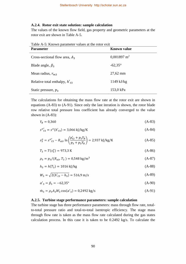
90

A.2.4. Rotor exit state solution: sample calculation


rotor exit are shown in Table A-5.

Table A-5: Known parameter values at the rotor exit



Blade angle, 𝛽3 -62,35°

Mean radius, 𝑟𝑚3 27,62 mm

Relative total enthalpy, ℎ′𝑡3 1149 kJ/kg


The calculations for obtaining the mass flow rate at the rotor exit are shown in

equations (A-83) to (A-91). Since only the last iteration is shown, the rotor blade

row relative total pressure loss coefficient has already converged to the value

shown in (A-83):

𝑌𝑅 = 0,360 (A-83)

𝑠𝑜𝑡3′

= 𝑠𝑜(ℎ′𝑡3) = 3,066 kJ/kg/K (A-84)

𝑠3𝑜 = 𝑠𝑜

𝑡3′ − 𝑅𝑎𝑖𝑟 ln (

𝑝𝑡2′ + 𝑝3𝑌𝑅

𝑝3 + 𝑝3𝑌𝑅) = 2,937 kJ/kg/K (A-85)

𝑇3 = 𝑇(𝑠3𝑜) = 973,3 K (A-86)

𝜌3 = 𝑝3/(𝑅𝑎𝑖𝑟 𝑇3 ) = 0,548 kg/m3 (A-87)

ℎ3 = ℎ(𝑇3) = 1016 kJ/kg (A-88)

𝑊3 = √2(ℎ′𝑡3 − ℎ3) = 516,9 m/s (A-89)

𝛼′3 = 𝛽3 = −62,35° (A-90)

�̇�3 = 𝜌3𝐴3𝑊3 cos(𝛼′3) = 0,2492 kg/s (A-91)

A.2.5. Turbine stage performance parameters: sample calculation

The turbine stage has three performance parameters: mass through flow rate, total-

to-total pressure ratio and total-to-total isentropic efficiency. The stage mass

through flow rate is taken as the mass flow rate calculated during the gas states

calculation process. In this case it is taken to be 0.2492 kg/s. To calculate the


91

total-to-total pressure ratio, the rotor exit total pressure is needed. The calculations

for obtaining the total-to-total pressure ratio are shown in equations (A-92) to (A-

98).

𝐶𝜃3 = 𝑊3 sin𝛼3′ + 𝑟𝑚3𝜔 = −110,8 m/s (A-92)

𝐶𝑧3 = 𝑊3 cos 𝛼3′ = 239,9 m/s (A-93)

𝐶3 = √𝐶𝜃32 + 𝐶𝑧3

2 = 264,2 m/s (A-94)

ℎ𝑡3 = ℎ3 +1

2𝐶3

2 = 1051 kJ/kg (A-95)

𝑠𝑡3𝑜 = 𝑠𝑜(ℎ𝑡3) = 2,972 J/kg/K (A-96)

𝑝𝑡3 = 𝑝3 exp (𝑠𝑡3

𝑜 − 𝑠3𝑜

𝑅𝑎𝑖𝑟) = 173,0 kPa (A-97)

𝑃𝑅𝑡𝑡 =𝑝𝑡0

𝑝𝑡3= 1,782 (A-98)

The ideal total stage exit enthalpy is required to calculate the total-to-total

isentropic efficiency of the turbine stage. It is calculated using isentropic relations

in equations (A-99) and (A-100).

Using equation (3.40), the total-to-total isentropic efficiency of the turbine stage is

calculated:

Appendix B: Turbine design process calculations

This appendix contains sample calculations for different stages of the design

procedure. As in Appendix A, the intrinsic ideal gas properties of air are related

by property table interpolations.

𝑠𝑡3,𝑖𝑑𝑒𝑎𝑙𝑜 = 𝑠𝑡0

𝑜 + 𝑅𝑎𝑖𝑟 ln (𝑝𝑡3

𝑝𝑡0) = 2,932 kJ/kg/K (A-99)

ℎ𝑡3,𝑖𝑑𝑒𝑎𝑙 = ℎ(𝑠𝑡3,𝑖𝑑𝑒𝑎𝑙𝑜 ) = 1011 kJ/kg (A-100)

𝜂𝑡𝑡 =ℎ𝑡0 − ℎ𝑡3

ℎ𝑡0 − ℎ𝑡3,𝑖𝑑𝑒𝑎𝑙= 0,7680 = 76,8 %. (A-101)


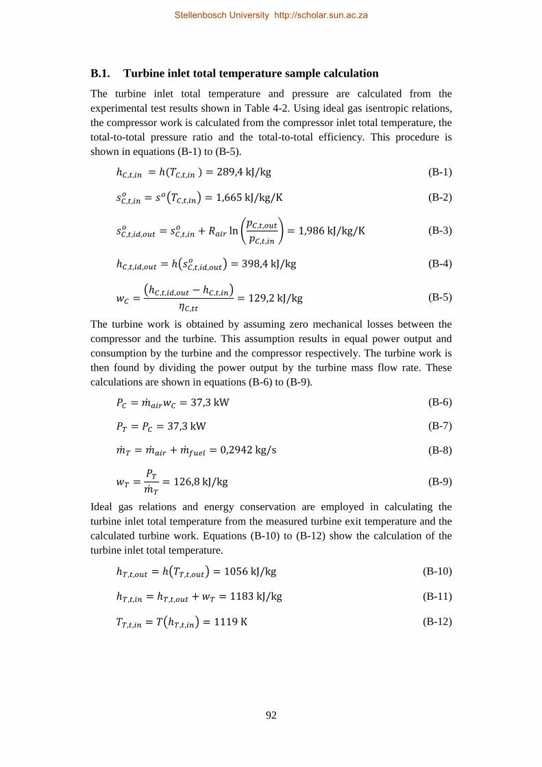
92

B.1. Turbine inlet total temperature sample calculation

The turbine inlet total temperature and pressure are calculated from the

experimental test results shown in Table 4-2. Using ideal gas isentropic relations,

the compressor work is calculated from the compressor inlet total temperature, the

total-to-total pressure ratio and the total-to-total efficiency. This procedure is

shown in equations (B-1) to (B-5).

ℎ𝐶,𝑡,𝑖𝑛 = ℎ(𝑇𝐶,𝑡,𝑖𝑛 ) = 289,4 kJ/kg (B-1)

𝑠𝐶,𝑡,𝑖𝑛𝑜 = 𝑠𝑜(𝑇𝐶,𝑡,𝑖𝑛) = 1,665 kJ/kg/K (B-2)

𝑠𝐶,𝑡,𝑖𝑑,𝑜𝑢𝑡𝑜 = 𝑠𝐶,𝑡,𝑖𝑛

𝑜 + 𝑅𝑎𝑖𝑟 ln (𝑝𝐶,𝑡,𝑜𝑢𝑡

𝑝𝐶,𝑡,𝑖𝑛) = 1,986 kJ/kg/K (B-3)

ℎ𝐶,𝑡,𝑖𝑑,𝑜𝑢𝑡 = ℎ(𝑠𝐶,𝑡,𝑖𝑑,𝑜𝑢𝑡𝑜 ) = 398,4 kJ/kg (B-4)

𝑤𝐶 =(ℎ𝐶,𝑡,𝑖𝑑,𝑜𝑢𝑡 − ℎ𝐶,𝑡,𝑖𝑛)

𝜂𝐶,𝑡𝑡= 129,2 kJ/kg (B-5)

The turbine work is obtained by assuming zero mechanical losses between the

compressor and the turbine. This assumption results in equal power output and

consumption by the turbine and the compressor respectively. The turbine work is

then found by dividing the power output by the turbine mass flow rate. These

calculations are shown in equations (B-6) to (B-9).

𝑃𝐶 = �̇�𝑎𝑖𝑟𝑤𝐶 = 37,3 kW (B-6)

𝑃𝑇 = 𝑃𝐶 = 37,3 kW (B-7)

�̇�𝑇 = �̇�𝑎𝑖𝑟 + �̇�𝑓𝑢𝑒𝑙 = 0,2942 kg/s (B-8)

𝑤𝑇 =𝑃𝑇

�̇�𝑇= 126,8 kJ/kg (B-9)

Ideal gas relations and energy conservation are employed in calculating the

turbine inlet total temperature from the measured turbine exit temperature and the

calculated turbine work. Equations (B-10) to (B-12) show the calculation of the

turbine inlet total temperature.

ℎ𝑇,𝑡,𝑜𝑢𝑡 = ℎ(𝑇𝑇,𝑡,𝑜𝑢𝑡) = 1056 kJ/kg (B-10)

ℎ𝑇,𝑡,𝑖𝑛 = ℎ𝑇,𝑡,𝑜𝑢𝑡 + 𝑤𝑇 = 1183 kJ/kg (B-11)

𝑇𝑇,𝑡,𝑖𝑛 = 𝑇(ℎ𝑇,𝑡,𝑖𝑛) = 1119 K (B-12)


93

The total pressure is assumed to remain constant throughout the combustion

chamber. Therefore, the turbine inlet total pressure is taken to be equal to the

compressor exit total pressure. This relation is shown in equation (B-13).

𝑝𝑇,𝑡,𝑖𝑛 = 𝑝𝐶,𝑡,𝑜𝑢𝑡 = 310 kPa (B-13)

B.2. Non-dimensional performance parameters sample calculation

The non-dimensional performance parameters are dependent on the axial gas

velocity through the turbine stage, the rotor blade speed, the exit flow angle and

the power absorbed. The latter three parameters are known from previous

calculations, which leaves the axial gas velocity to be calculated. The axial gas

velocity is dependent on the mass flow rate, the static gas density and the flow

area at a given cross section. The flow area is calculated from the stage inlet

geometry specified in Table 4.1:

𝐴0 = 𝜋(𝑟𝑠02 − 𝑟ℎ0

2 ) = 3,46(10)−4 m2 (B-14)

Since the turbine inlet total gas properties are specified in Table 4.3, the static

flow properties can be calculated using the mass flow rate obtained in equation

(B-8). In equations (B-15) and (B-16), the static density of the gas at the turbine

inlet is approximated by assuming it to equal the total gas density. This density is

then used in equation (B-17) with the known inlet flow area and mass flow rate to

obtain an inlet axial velocity estimate. Since a purely axial inlet velocity has been

chosen, the velocity magnitude equals the axial velocity. Therefore, the velocity

estimate, together with the known total thermodynamic properties, can be used to

find the static density, as shown in equations (B-18) to (B-22).

𝜌0,𝑒𝑠𝑡𝑖𝑚𝑎𝑡𝑒 = 𝑝𝑡0/(𝑅𝑎𝑖𝑟𝑇𝑡0) = 0,965 kg/m3 (B-15)

𝜌0 = 𝜌0,𝑒𝑠𝑡𝑖𝑚𝑎𝑡𝑒 (B-16)

𝐶0 = �̇�𝑡𝑢𝑟𝑏𝑖𝑛𝑒/(𝜌0𝐴0) = 217 m/s (B-17)

ℎ0 = ℎ𝑡0 − 𝐶02/2 = 1160 kJ/kg (B-18)

𝑇0 = 𝑇(ℎ0) = 1100 K (B-19)

𝑠0𝑜 = 𝑠𝑜(𝑇0) = 3,08 kJ/kg/K (B-20)

𝑝0 = 𝑝𝑡0 exp[(𝑠0𝑜 − 𝑠𝑡0

𝑜 )/𝑅𝑎𝑖𝑟] = 288 kPa (B-21)

𝜌0 = 𝑝0/(𝑅𝑎𝑖𝑟𝑇0) = 0,913 kg/m3 (B-22)

The density obtained in equation (B-22) can then be used as a new static density

estimate in equation (B-17). The calculation of equations (B-17) to (B-22) is


94

repeated until the calculated value of the static inlet density has converged. For

the values in this sample calculation, the converged static density and axial

velocity are 0,906 kg/m3 and 232 m/s respectively. The non-dimensional flow

coefficient, work coefficient and reaction ratio are then calculated in equations (B-

23) to (B-25).

𝜙𝑚𝑒𝑎𝑛 = 𝐶𝑚/𝑈 = 𝐶𝑚/(𝑟𝑚𝑒𝑎𝑛𝜔𝑡𝑢𝑟𝑏𝑖𝑛𝑒) = 0,670 (B-23)

𝜓𝑚𝑒𝑎𝑛 = ∆ℎ0/𝑈2 = (𝑃𝑡𝑢𝑟𝑏𝑖𝑛𝑒/�̇�𝑡𝑢𝑟𝑏𝑖𝑛𝑒 )/(𝑟𝑚𝑒𝑎𝑛𝜔𝑡𝑢𝑟𝑏𝑖𝑛𝑒)2

= 1,07 (B-24)

𝑅𝑚𝑒𝑎𝑛 = 1 − 𝜙𝑚𝑒𝑎𝑛 tan 𝛼3,𝑚𝑒𝑎𝑛 − 𝜓𝑚𝑒𝑎𝑛/2 = 0,466 (B-25)

B.3. Mean radius gas velocity triangle calculations

For a constant radius stream sheet, the blade speed remains constant across a

blade row. Therefore, since the mean radius remains constant throughout the

turbine stage,

𝑊𝜃2,𝑚𝑒𝑎𝑛 − 𝑊𝜃3,𝑚𝑒𝑎𝑛 = 𝐶𝜃2,𝑚𝑒𝑎𝑛 − 𝐶𝜃3,𝑚𝑒𝑎𝑛. (B-26)

The stage flow and work coefficients are defined as:

𝜙𝑚𝑒𝑎𝑛 =𝐶𝑧,𝑚𝑒𝑎𝑛

𝑈𝑚𝑒𝑎𝑛 (B-27)

and

𝜓𝑚𝑒𝑎𝑛 =∆ℎ𝑡

𝑈𝑚𝑒𝑎𝑛2 . (B-28)

Applying Euler’s turbine equation and equation (B-26), the stage work coefficient

can be written as either

𝜓𝑚𝑒𝑎𝑛 =𝐶𝜃2,𝑚𝑒𝑎𝑛 − 𝐶𝜃3,𝑚𝑒𝑎𝑛

𝑈𝑚𝑒𝑎𝑛, (B-29)

or

𝜓𝑚𝑒𝑎𝑛 =𝑊𝜃2,𝑚𝑒𝑎𝑛 − 𝑊𝜃3,𝑚𝑒𝑎𝑛

𝑈𝑚𝑒𝑎𝑛. (B-30)

The stage reaction ratio is defined as the ratio of the static enthalpy drop across

the rotor blade row to the total enthalpy drop across the whole stage.

𝑅𝑚𝑒𝑎𝑛 =ℎ2 − ℎ3

∆ℎ𝑡. (B-31)

Using the definition of total enthalpy and considering that all of the stage work is

done on the rotor blade row; this expression can be rewritten as


95

𝑅𝑚𝑒𝑎𝑛 =ℎ𝑡2 − ℎ𝑡3 −

12 (𝐶2,𝑚𝑒𝑎𝑛

2 − 𝐶3,𝑚𝑒𝑎𝑛2 )

∆ℎ𝑡

=∆ℎ𝑡 −

12 (𝐶2,𝑚𝑒𝑎𝑛

2 − 𝐶3,𝑚𝑒𝑎𝑛2 )

∆ℎ𝑡.

(B-32)

By applying Euler’s turbine equation and breaking the gas velocities up in

orthogonal components, the turbine stage reaction ratio can be written as:

𝑅𝑚𝑒𝑎𝑛 = 1 +𝐶𝜃2,𝑚𝑒𝑎𝑛 − 𝐶𝜃3,𝑚𝑒𝑎𝑛

2𝑈𝑚𝑒𝑎𝑛−

𝐶𝜃2,𝑚𝑒𝑎𝑛

𝑈𝑚𝑒𝑎𝑛

= 1 +1

2

𝐶𝜃2,𝑚𝑒𝑎𝑛 − 𝐶𝜃3,𝑚𝑒𝑎𝑛

𝑈𝑚𝑒𝑎𝑛−

𝐶𝑧,𝑚𝑒𝑎𝑛 𝑡𝑎𝑛 𝛼2,𝑚𝑒𝑎𝑛

𝑈𝑚𝑒𝑎𝑛 .

(B-33)

Substituting equations (B-27) and (B-29) into equation (B-33) allows the stage

exit angle to be expressed as:

𝛼2,𝑚𝑒𝑎𝑛 = tan−1 (1 − 𝑅𝑚𝑒𝑎𝑛 +



). (B-34)

It can similarly be shown by substituting equations (B-26) and (B-30) into

equation (B-33) that the rotor relative inlet and exit flow angles are given by

equations (4.6) and (4.7).

Table B-1: Calculated turbine stage gas velocities

Location,

𝒊

Absolute

flow angle,

𝜶𝒊

Absolute gas

velocity

magnitude, 𝑪𝒊

Relative

flow angle,

𝜶𝒊′

Relative gas

velocity

magnitude, 𝑾𝒊

0 0 ° 237 m/s 0 ° 237 m/s

1 57,1 ° 437 m/s 57,1 ° 437 m/s

2 57,1 ° 437 m/s 5,15 ° 238 m/s

3 0 ° 237 m/s -55.6 ° 419 m/s

B.4. Turbine gas states sample calculation

This is a sample calculation of the gas states throughout the turbine stage. The gas

states are calculated from the stage inlet total gas properties in Table 4-3, the

mean radius gas velocities in Table B-1, and stator and rotor blade row total


96

pressure loss coefficients of 0,085 and 0,166 respectively. Since the both the

relative and the absolute gas velocities are known throughout the turbine stage,

the definitions of total enthalpy and relative total enthalpy are used throughout the

calculations to interrelate the static, total and relative total enthalpies.

B.4.1. State 0 calculation

The turbine stage inlet static gas conditions are calculated from the turbine inlet

total temperature and pressure, and the turbine inlet velocity. The definition of

total enthalpy is used to relate the total state to the static state in equation (B-37).

Variable specific heat isentropic ideal gas relations are then used to relate the

static pressure to the total pressure in equation (B-40). With the static state

known, the sonic velocity and gas density at the stator inlet are calculated in

equations (B-41) and (B-42) respectively.

ℎ𝑡0 = ℎ(𝑇𝑡𝑜) = 1183 kJ/kg (B-35)

𝑠𝑡0𝑜 = 𝑠𝑜(𝑇𝑡𝑜) = 3,097 kJ/kg/K (B-36)

ℎ0 = ℎ𝑡0 −1

2𝐶0

2 = 1155 kJ/kg (B-37)

𝑇0 = 𝑇(ℎ0) = 1095 K (B-38)

𝑠0𝑜 = 𝑠𝑜(𝑇0) = 3,072 kJ/kg/K (B-39)

𝑝0 = 𝑝𝑡0 exp (𝑠0

𝑜 − 𝑠𝑡0𝑜

𝑅𝑎𝑖𝑟) = 284 kPa (B-40)

𝑎0 = √𝛾(𝑇0) 𝑅𝑎𝑖𝑟 𝑇0 = 657 m/s (B-41)

𝜌0 =𝑝0

𝑅𝑎𝑖𝑟 𝑇0= 0,903 kg/m3 (B-42)


Assuming conservation of total enthalpy, the total enthalpy is known at the stator

exit. The definition of total enthalpy is used to obtain the static enthalpy in

equation (B-44). The stator total pressure loss coefficient is then used in equation

(B-47) to calculate the static pressure. The sonic velocity and density are then

calculated as before in equations (B-49) and (B-50) respectively.

ℎ𝑡1 = ℎ𝑡0, 𝑇𝑡1 = 𝑇𝑡0, 𝑠𝑡1𝑜 = 𝑠𝑡0

𝑜 (B-43)


97

ℎ1 = ℎ𝑡1 −1

2𝐶1

2 = 1088 kJ/kg (B-44)

𝑇1 = 𝑇(ℎ1) = 1036 K (B-45)

𝑠1𝑜 = 𝑠𝑜(𝑇1) = 3,009 kJ/kg/K (B-46)

𝑝1 =𝑝𝑡0

(1 + 𝑌𝑆) exp (𝑠𝑡1

𝑜 − 𝑠1𝑜

𝑅𝑎𝑖𝑟) − 𝑌𝑆

= 222,6 kPa (B-47)


𝑜 − 𝑠1𝑜

𝑅𝑎𝑖𝑟) = 303,1 kPa (B-48)

𝑎1 = √𝛾(𝑇1) 𝑅𝑎𝑖𝑟 𝑇1 = 639,8 m/s (B-49)

𝜌1 =𝑝1

𝑅𝑎𝑖𝑟 𝑇1= 0,748 kg/m3 (B-50)


The total and static thermodynamic properties are assumed to remain constant

from the stator exit to the rotor inlet. However, the relative total properties do

change due to the motion of the rotor. The definition of the relative total enthalpy

and variable specific heat isentropic ideal gas relations are used to determine the

relative total state in equations (B-53) and (B-56).

ℎ𝑡2 = ℎ𝑡1, 𝑇𝑡2 = 𝑇𝑡1, 𝑠𝑡2𝑜 = 𝑠𝑡1

𝑜 , 𝑝𝑡2 = 𝑝𝑡1 (B-51)

ℎ2 = ℎ1, 𝑇2 = 𝑇1, 𝑠2𝑜 = 𝑠1

𝑜 , 𝑝2 = 𝑝1 (B-52)

ℎ𝑡2′ = ℎ2 +

1

2𝑊2

2 = 1116 kJ/kg (B-53)

𝑇𝑡2′ = 𝑇(ℎ𝑡2

′ ) = 1061 K (B-54)

𝑠𝑡2𝑜′

= 𝑠𝑜(𝑇𝑡2′ ) = 3,036 kJ/kg/K (B-55)


𝑠𝑡2𝑜′

− 𝑠2𝑜

𝑅𝑎𝑖𝑟) = 244,5 kPa (B-56)


Assuming constant radius flow, the relative total enthalpy stays conserved across

the rotor blades. Therefore, the static enthalpy at the rotor exit is found from the

definition of relative total enthalpy in equation (B-58). Similarly to the stator exit


98

static pressure, in equation (B-61) the rotor exit static pressure is obtained using

the rotor relative total pressure loss coefficient and the variable specific heat

isentropic ideal gas relations. The latter is utilised again in equation (B-66) to

obtain the total pressure at the rotor exit. The sonic velocity and gas density are

found as before in equations (B-67) and (B-68).

ℎ𝑡3′ = ℎ𝑡2

′ , 𝑇𝑡3′ = 𝑇𝑡2

′ , 𝑠𝑡3𝑜′

= 𝑠𝑡2𝑜′

(B-57)

ℎ3 = ℎ𝑡3′ −

1

2𝑊3

2 = 1028 kJ/kg (B-58)

𝑇3 = 𝑇(ℎ3) = 984,3 K (B-59)

𝑠3𝑜 = 𝑠𝑜(𝑇3) = 2,950 kJ/kg/K (B-60)

𝑝3 =𝑝𝑡2

′

(1 + 𝑌𝑅) exp (𝑠𝑡3

𝑜′− 𝑠3

𝑜

𝑅𝑎𝑖𝑟) − 𝑌𝑅

= 173,8 kPa (B-61)


𝑠𝑡3𝑜′

− 𝑠3𝑜

𝑅𝑎𝑖𝑟) = 234,5 kPa (B-62)

ℎ𝑡3 = ℎ3 +1

2𝐶3

2 = 1056 kJ/kg (B-63)

𝑇𝑡3 = 𝑇(ℎ𝑡3) = 1009 K (B-64)

𝑠𝑡3𝑜 = 𝑠𝑜(𝑇𝑡3) = 2,978 kJ/kg/K (B-65)


𝑜 − 𝑠3𝑜

𝑅𝑎𝑖𝑟) = 191,8 kPa (B-66)

𝑎3 = √𝛾(𝑇3) 𝑅𝑎𝑖𝑟 𝑇3 = 624,1 m/s (B-67)

𝜌3 =𝑝3

𝑅𝑎𝑖𝑟 𝑇3= 0,615 kg/m3 (B-68)

Since both the gas velocities and thermodynamic states throughout the turbine are

known, equation (B-69) is used to calculate the absolute and relative Mach

numbers throughout the turbine. These calculated values are shown in Table B-2.

𝑀𝑖′ =

𝑊𝑖

𝑎𝑖 (B-69)


99

Table B-2: Calculated turbine stage gas Mach numbers

Location,

𝒊 Absolute Mach number, 𝑴𝒊 Relative Mach number, 𝑴𝒊

′

0 0,36 0,36

1 0,68 0,68

2 0,68 0,37

3 0,38 0,67

B.5. Blade row geometric parameters – sample calculations

This is a sample calculation of the blade parameters of a rotor blade row during

the design process. The calculation uses the flow angles and Mach numbers given

in Tables B-1 and B-2 respectively and uses the gas states calculated in section

B.4. The calculation also uses the geometrical design parameters given in Table 4-

1. The optimal pitch-to-chord ratio is first calculated, and then the other blade row

geometric parameters are determined.

B.5.1. Calculating the optimal pitch-to-chord ratio

Firstly, the relative flow angles before and after the rotor blade row obtained in

section B.3 are transformed into the generic blade angle convention using

equations (1.3) and (1.4).

𝛼𝑏2′ = 90° − 𝛼2

′ = 84,85° (B-70)

𝛼𝑏3′ = 90° + 𝛼3

′ = 34,4° (B-71)

The optimal pitch-to-chord ratio is now determined by first calculating the

optimal pitch-to-chord ratios for nozzle and impulse blades with the the given

relative exit flow angle in equations (B-73) and (B-74) respectively. The gas

deflection ratio, obtained in equation (B-72), is then used to interpolate between

these two values in equation (B-75), thus yielding the optimal pitch-to-chord ratio.

(Aungier, 2006)

𝜉 =90° − 𝛼𝑏2

′

90° − 𝛼𝑏3′ = 0,0926 (B-72)

(𝑠/𝑐)𝑛𝑜𝑧𝑧𝑙𝑒 = 0.427 +𝛼𝑏3

′

58°− (

𝛼𝑏3′

93°)

2

= 0,883 (B-73)


100

(𝑠/𝑐)𝑖𝑚𝑝𝑢𝑙𝑠𝑒 = 0.224 + (1.575 −𝛼𝑏3

′

90°) (

𝛼𝑏3′

90°) = 0,680 (B-74)

(𝑠/𝑐)𝑜𝑝𝑡 = (𝑠/𝑐)𝑛𝑜𝑧𝑧𝑙𝑒 + [(𝑠/𝑐)𝑛𝑜𝑧𝑧𝑙𝑒 − (𝑠/𝑐)𝑖𝑚𝑝𝑢𝑙𝑠𝑒]|𝜉|𝜉 = 0,882 (B-75)

B.5.2. Determining the blade pitch, chord and stagger angle

The blade pitch, chord and stagger angle are calculated iteratively. However, the

pitch-to-chord ratio depends on the stream sheet area ratio correction factor,

calculated in equation (B-75), which is unaffected by the other variables.

𝐹𝐴𝑅 = 0,8 + 0,2 (𝜌2 𝐶𝑧2

𝜌3 𝐶𝑧3) = 0,8 + 0,2 (

𝜌2

𝜌3) = 1,04 (B-75)

As a starting point for the iterative procedure for satisfying equations (4.21),

(4.25), (4.24) and (4.23), a zero deviation angle is assumed. However, the

calculated deviation angle converges to a value of 𝛿 = 1,92°. Therefore, for the

final iteration shown in equations (B-76) to (B-79), the converged value is used.

(𝑜/𝑠) = 𝐹𝐴𝑅 sin(𝛼𝑏3′ − 𝛿) = 0,56 (B-76)

𝛽𝑔 = sin−1(𝑜/𝑠) = 34,1° (B-77)

𝛿0 = sin−1 {(𝑜/𝑠)[1 + (1 − 𝑜/𝑠)] (𝛽𝐺

90°) } − 𝛽𝐺 = 2,48° (B-78)

𝛿 = {𝛿0, 𝑀3

′ ≤ 0,5

𝛿0(1 − 10(2𝑀3′ − 1)3 + 15(2𝑀3

′ − 1)4 − 6(2𝑀3′ − 1)5), 𝑀3

′ > 0,5= 1.92°

(B-79)

The stagger angle is now calculated using equation (4.26). The blade chord is then

calculated in equation (B-81), enabling the calculation of the blade pitch in

equation (B-82) and subsequently the number of blades in equation (B-83).

𝛾 =(180° − 𝛽2 + 1.5𝛽𝑔)

2.5= 58,5° (B-80)

𝑐 =𝑏𝑧𝑟

𝑠𝑖𝑛(𝛾)= 8,21 𝑚𝑚 (B-81)

𝑠 = 𝑐 (𝑠/𝑐)𝑜𝑝𝑡 = 7,24 mm (B-82)

𝑁 =2𝜋𝑟𝑚

𝑠= 23,9 (B-83)


101

Since a prime number of blades is preferable, the blade number is rounded down

to 23.


102

Appendix C: CFD verification

C.1. Inlet and outlet block length independence

This section illustrates the inlet and outlet domain length independence of the

flow solutions obtained during the CFD performance analysis. The inlet and outlet

sections act as buffer zones between the turbine blade rows and the domain inlet

and outlet surfaces. The inlet and outlet section lengths must therefore be long

enough to prevent the constant property and zero gradient boundary conditions

from influencing the flow field near the blades.

To determine whether the inlet and outlet section lengths are long enough, three

different lengths for the inlet and outlet sections are simulated. The three

simulations have constant values for the other flow simulation parameters, and

computational meshes of similar elements counts. The results of the three

simulations are shown in Table. The simulated mass flow rate through the turbine

and the total-to-total stage efficiency are shown for different inlet and outlet

domain lengths.

Table C-1: Domain length independence study results

Inlet and outlet domain

lengths

Simulated turbine mass

flow rate, kg/s

Simulated turbine total-

to-total efficiency

5 mm 0,287 91,7 %

10 mm 0,287 91,8 %

20 mm 0,287 91,7 %

It can be seen in Table that doubling the inlet and outlet domain lengths first from

5 mm to 10 mm and then again to 20 mm has very little effect on the measured

parameters. It is therefore concluded that inlet and outlet lengths of 10 mm can be

used with minimal influence on the flow field around the turbine blades.

C.2. Computational mesh independence

This section illustrates the mesh density independence of the flow solutions

obtained during the CFD performance analysis. This is done by simulating the

same flow problem using three computational meshes with different element

counts. Simulation B of the 95 % work coefficient design is solved using three

computational meshes consisting of roughly 100,000, 200,000 and 400,000

elements respectively. The results of the three simulations are shown in Table.


103

The simulated mass flow rate through the turbine and the total-to-total stage

efficiency are shown for each mesh element count.

Table C-2: Mesh independence study results

Number of mesh

elements

Simulated turbine mass

flow rate, kg/s

Simulated turbine total-

to-total efficiency

119 595 0,287 92,1 %

212 630 0,288 91,8 %

424 844 0,285 92,3 %

It is clear from Table that varying the mesh density in between element counts of

approximately 100,000, 200,000 and 400,000 has little effect on the predicted

mass flow rate or total-to-total efficiency. Therefore, it is concluded that a

computational mesh element count of approximately 200,000 can be used with

confidence to generate mesh independent results.


104

Appendix D: FEM analysis information

D.1. Material properties of Inconel IN713 LC

Table D-1: Mechanical properties of Inconel IN713 LC (Nickel Development

Institute, 1995)

Density, kg/m3 8000

Poisson’s ratio (Creci, et al., 2010) 0,382

Temperature,

K

Thermal expansion

coefficient, μm/m°C

Modulus of

elasticity, GPa

Yield strength,

MPa

294 - 197 750

366 10,1 194 -

477 12,6 186 -

589 13,7 183 -

700 14,9 178 -

811 15,8 172 760

922 16 165 785

1033 10,1 159 760

1144 16,2 149 580

1255 16,7 136 285

1366 17 - -

1033 18,9 - -

D.2. FEM mesh convergence studies

D.2.1. Mesh independence of static structural analyses

To investigate the dependence of the static structural analysis results on the

computational mesh element size, a mesh independence study is performed. Static

structural analyses of the 95 % work coefficient turbine design are performed

using computational meshes with different element counts. The mesh element

count and the resulting tip displacement and maximum Von-Mises stress of each

simulation are shown in Table.


105

Table D-2: Static structural mesh independence study results

The blade tip displacement does not change between the different simulations, but

the maximum Von-Mises stress does change markedly for the first three

simulations. Thereafter the maximum Von-Mises stress remains fairly constant.

Therefore, it is concluded that a mesh element count of approximately 45,000 is

sufficient to obtain mesh independent static structural analysis results.

D.2.2. Mesh independence of structural modal analyses

A mesh independence study is also performed to investigate the dependence of the

modal structural analysis results on the computational mesh element size. Modal

structural analyses of the 95 % work coefficient turbine design are performed

using computational meshes with different element counts. The mesh element

count and the resulting first three blade natural frequencies of each simulation are

shown in Table.

Table D-3: Modal analysis mesh independence study results

The computed natural frequencies do not change between the different

simulations. Therefore, it is concluded that a mesh element count of

approximately 45,000, as used for the static structural analyses, is also sufficient

to obtain mesh independent modal analysis results.

Number of mesh

elements

Total tip displacement,

mm

Max. von-mises root

stress, MPa

14,994 0,330 738

22,923 0,330 743

45,182 0,330 710

93,117 0,330 707

168,354 0,330 709

Number of mesh

elements

1st natural

frequency

2nd natural

frequency

3rd natural

frequency

14,999 6,57 kHz 15,2 kHz 23,3 kHz

23,182 6,57 kHz 15,2 kHz 23,3 kHz

45,046 6,57 kHz 15,2 kHz 23,3 kHz


106

References

Ainley, D. G. & Mathieson, G. C. R., 1951. A method of performance estimation

of axial-flow turbines, London: Her Majesty's Stationary Office.

Aungier, R. H., 2006. Turbine aerodynamics. 1st ed. New York: ASME press.

Baskharone, E. A., 2006. Principles of turbomachinery in air-breathing engines.

New York: Cambridge University Press.

Cengel, Y. A. & Boles, M. A., 2004. Thermodynamics: an engineering approach.

Boston: McGraw-Hill Professional Publishing.

Chen, L.-C. & Lin, G. C. I., 2000. Reverse engineering in the design of turbine

blades - a case study in applying the MAMDP. Robotics and Computer Integrated

Manufacturing, pp. 161-167.

Chivate, P. N. & Jablokow, A. G., 1995. Review of surface representations and

fitting for reverse engineering. Computer Integrated Manufacturing Systems, pp.

193-204.

Cohen, H., Rogers, G. F. C. & Saravanamuttoo, H. I. H., 1996. Gas turbine

theory. Harlow: Longman Group Limited.

Creci, G., Menezes, J. C., Barbosa, J. R. & Corra, J. A., 2010. Rotor-bearing

analysis of a single spool gas turbine by considering bearing stiffness and

damping dynamics. Campina Grande, Brazilian Association of Mechanical

Sciences and Engineering.

De la Calzada, P., 2011. Profile loss coefficient definitions revisited. International

Journal of Turbo Jet-Engines, pp. 209-225.

De Wet, A. L., 2011. Performance investigation of a turbocharger compressor.

Stellenbosch: Stellenbosch University.

Dixon, S. L., 1998. Fluid Mechanics and Thermodynamics of Turbomachinery.

4th ed. Oxford: Butterworth-Heinemann.

Djouimaa, S., Messaoudi, L. & Giel, P. W., 2007. Transonic turbine loading

calculations using different turbulence models - effects of reflection and non-

reflecting boundary conditions. Applied Thermal Engineering, pp. 779-787.


107

Dong, Y.-w., Bu, K., Dou, Y.-q. & Zhang, D.-h., 2011. Determination of a wax

pattern die profile for investment casting of turbine blades. Transactions of

Nonferrous Metal Society of China, pp. 378-387.

Japikse, D. & Baines, N. C., 1994. Introduction to turbomachinery. 1st ed.

Oxford: Oxford university press.

Junhui, H., Zhao, W., Jianmin, G. & Yu, Y., 2010. Overview of the profile

measurement of a turbine blade and its development. Wollongong, SPIE, pp.

76560L-1 - 76560L-11.

Korakianitis, T. & Papagiannidis, P., 1993. Surface curvature distribution effects

on turbine cascade performance. Journal of Turbomachinery, 2(115), pp. 334-341.

Krige, D. S., 2012. Performance evaluation of a micro gas turbine centrifugal

compressor diffuser. Stellenbosch: Stellenbosch University.

Lau, Y. L., Leung, R. C. K. & So, R. M. C., 2007. Vortex-induced vibration effect

on fatigue life estimate of turbine blades. Journal of Sound and Vibration, pp.

698-719.

Mitchell, N. A., 1982. The preliminary analysis of axial turbines by a simplified

throughflow procedure. Journal of Mechanical Engineering Science, pp. 5-10.

Mohaghegh, K., Sadeghi, M. H. & Abdullah, A., 2006. Reverse engineering of

tubine blades based on design intent. International Journal of Advanced

Manufacturing Technology, pp. 1009-1020.

Nickel Development Institute, 1995. High-temperature high-strength Nickel base

alloys (393). [Online]

Available at: http://www.nickelinstitute.org/~/Media/Files/TechnicalLiterature/

High_TemperatureHigh_StrengthNickel_BaseAlloys_393_.pdf#page=

[Accessed 21 September 2012].

Smith, S. F., 1965. A simple correlation of turbine efficiency. Journal of Royal

Aeronautical Society, Issue 69, pp. 467-470.

Struwig, D., 2012. Design and construction of a test bench for micro

turbomachinery. Stellenbosch: Stellenbosch University.


108

Van der Merwe, B. B., 2012. Design of a centrifugal compressor impeller for

micro gas turbine application. Stellenbosch: Stellenbosch University.

Wesssels, F., Venter, G. & Von Backström, T., 2012. An efficient scheme for

describing airfoils using non-uniform rational B-splines. Copenhagen, American

Society of Mechanical Enigneers.

Wilson, D. G., 1987. New guidelines for the preliminary design and performance

prediction of axial-flow turbines. Proceedings of the Institution of Mechanical

Engineers, Part A: Journal of Power and Energy, pp. 279-290.


design methodology of an axial flow turbine for a micro

Documents