design methodology based on h∞ control theory for marine ... · marine propulsion system with...

Design Methodology Based on H∞ Control Theory for

Marine Propulsion System with Bumpless Transfer Function

M. J. LOPEZ, L. GARCIA, J. LORENZO, A. CONSEGLIERE

Departamento de Ingeniería de Sistemas y Automática

Universidad de Cádiz

Centro Andaluz Superior Estudios Marinos (CASEM)

SPAIN

{manueljesus.lopez, luis.garcia, jose.lorenzo, agustin.consegliere}@uca.es

http://www2.uca.es/dept/isa-tee/

Abstract: - In this paper we propose a control system design methodology which has two main objectives: the

first one is to achieve control system specifications for a local H∞ controller designed for a given operation

condition, and the second objective is to provide a procedure for bumpless transfer (BLT) when the controller is

switched to another one, due to change in the operation condition, or when the controller is retuned by a plant

operator. For that, the design procedure calculates a feedback H-controller (FB-HC) and an associated bump-less

transfer H-controller (BLT-HC). The method is implemented in an auto-tuning procedure, where both pre-

tuning controllers (FB-HC and BLT-HC) are obtained in a systematic manner. Controllers fine-tuning can be

carried out by a plant operator using two tuning parameters and several tuning rules. Our design methodology is

applied to a marine propulsion system with diesel engine used as propeller prime-mover. Due to different

operation regimens of ship propulsion, several linear controllers are designed for different operating points,

switching (with bumpless-transfer) between them when is necessary; which enables the system to be controlled

satisfactorily within the whole of its operating range. Satisfactory results are obtained by simulations with the

nonlinear model of a merchant ship, and our hardware in the loop simulation (HILS) environment is described.

Key-Words: - ship propulsion system, H controller, bumpless transfer

1 Introduction When a controller is designed and implemented for

an industrial or marine process, on-line changes in

controller are required to adapt control system to new

situations [1,2,3,4,5]. The problem of bumpless

transfer refers to the instantaneous switching between

two controllers of a process while retaining a smooth

("bumpless") control signal. Avoiding transients after

switching from a controller to other one can be

viewed as an initial condition problem on the output

of the feedback controller. In process control and

marine systems there are several practical situations

that may all be interpreted as bumpless transfer

problems. These are:

1. Switching between manual an automatic control.

The ability to switch between manual and automatic

control while retaining a smooth control signal is the

traditional bumpless transfer problem.

2. Controller tuning. It is frequently desired to tune

controller parameters on-line and in response to

experimental observations.

3. Scheduled and adaptive controllers. Scheduled

controllers are controllers with time-varying

parameters. These time variations are usually due to

measured time-varying process parameters or due to

local linearization in different operating ranges.

4. Tentative evaluation of new controllers. This is a

challenging, and only recently highlighted bumpless

transfer scenario. It is motivated by the need to test

tentative controller designs safely and economically

on industrial and marine processes during normal

operation.

Consider, for example, a process operating in closed

loop with an existing controller. Assume that the

performance is unsatisfactory, and that a number of

new controller candidates have been designed and

simulated. It is then desired to test these controllers,

tentatively, on the plant to assess their respective

performances. Frequently it is not possible or feasible

to shut down the plant intermittently, and the

alternative controllers therefore have to be brought

on-line with a bumpless transfer mechanism during

normal plant operation.

Controller design for marine systems are mainly

based on PID technology [1,2,3,4,5,6], nevertheless,

if advanced control strategies are used, some

improved results can be obtained. In this work we

propose a method based on H∞ control theory, which

is complemented with a method for bumples transfer

WSEAS TRANSACTIONS on SYSTEMS M. J. Lopez, L. Garcia, J. Lorenzo, A. Consegliere

ISSN: 1109-2777 253 Issue 3, Volume 9, March 2010

(BLT) when controller switching is needed. The

method for BLT is also based on H∞ control theory,

but it is applied to PID controllers. Our design

methodology for controller design and BLT is

proved by means of simulation tests with the

propulsion system of a merchant ship.

Diesel engine is used as propeller prime-mover for

the majority of modern merchant ships. This is due to

three major reasons: 1) the superior (thermal)

efficiency of Diesel engines, b) large Diesel engines

can burn heavy fuel oil (HFO), c) slow-speed Diesel

engines can be directly connected to the propeller

without the need of gearbox and/or clutch and are

reversible. As shortcoming, Diesel engines require a

large engine room compared to gas turbines, which

can be a problem when extremely large power

outputs are required for large high-speed vessels

[1,2].

In this work, robust control theory results are

applied to design the propulsion control system of a

merchant ship. We employ a mathematical model

which is a synthesis of different models given in

literature [1,2,3,4,5,6], a nonlinear model which

captures the essential characteristics of ship

propulsion dynamics and it is used in order to carry

out real time hardware in the loop simulations

(HILS) [7,8,9,10]. Linearized models are used to

design PID and H∞ controllers [1,2,3,4,10,11,12] for

different operation conditions. To change controller

parameters without bump effect we propose a bump-

less procedure, which is applicable for controller

switching in gain scheduling method used for

adapting controller to changes in plant dynamics.

The rest of this paper is organized as follows: in

section two the system propulsion model is described,

the controller design methodology is outlined in

section three, simulation results are depicted in

section four, and finally concluding remarks are

given in section five.

2 Propulsion system model The propulsion system consists of two basic control

loops, one for propeller pitch (pitch controller) and

one for shaft speed (shaft speed controller). The

propulsion set-point is performed by a lever, named

“the telegraph”, placed on the bridge. Each lever

position corresponds, via the combinatory curve, to a

pitch setting and to the required rotational speed of

the engine. The reference signals are then transmitted

to the controller (named governor). The governor

inputs are the requested (set-point) and the actual

engine speeds, as well as the propeller pitch and its

set-point are used. The governor controls the fuel

flow to the cylinders in order to maintain the required

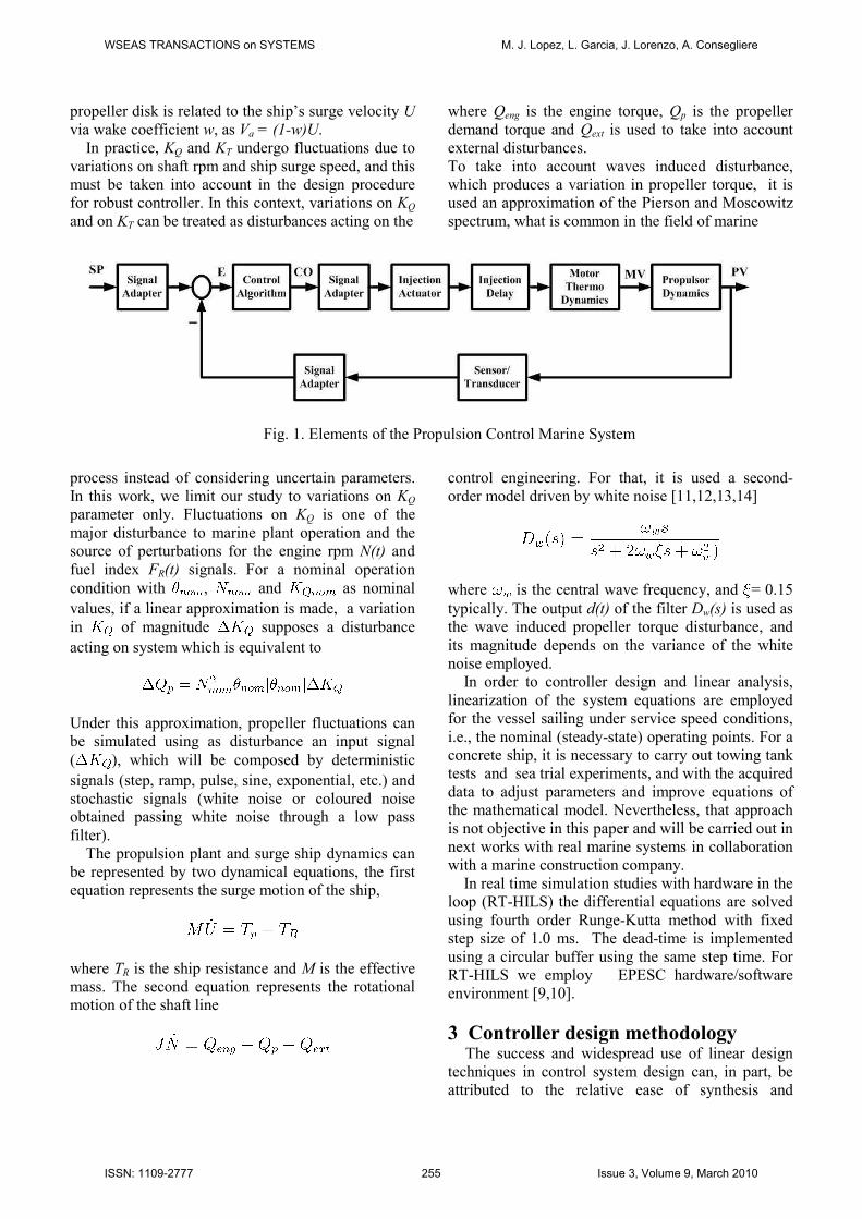
engine speed (see Fig.1).

Diesel engine of the prime-mover is modelled

taking into account the following components (see

block diagram of Fig. 1, where the basic signals and

elements of the control system are shown): 1) the

input signal produced by the controller (controller

output, CO) is first converted to an equivalent current

signal that drives the actuator. The injection actuator

has a time constant (as nominal value = 0.1 sec.

is used in simulations) that is dependent on the oil

temperature. The output of this unit is the fuel-flow,

which is a direct input to the engine. The injection

process is characterised by a dead-time (injection

delay) , which is a non-linear function of the

engine speed [1,2,3,14]

which has been estimated to lie within the range:

where z is the number of engine cylinders.

To model the engine thermodynamic process that

determines engine brake torque (manipulated

variable, MV in Fig. 1), a first order transfer function

with thermodynamic gain KTC and time constant τTC

is considered [2,3,4]

where FR is the named fuel index (rack) position or

fuel-rack position, in this equation is mainly due

to the effect of turbo-charging on the power

generation process. As nominal value it is used

seconds in simulations. Propeller thrust

and torque are modelled by means of

where θ is the propeller pitch ratio, and

vary with propeller shaft-speed (process variable,

PV in Fig. 1), and advance velocity , and can be

approximated as a n-th order polynomial in advance

number . Usually, a first order polynomial

or second order polynomial are employed

[15,16,17,18], where D is the propeller diameter, and

advance velocity Va of the water-flow over the



propeller disk is related to the ship’s surge velocity U

via wake coefficient w, as Va = (1-w)U.

In practice, KQ and KT undergo fluctuations due to

variations on shaft rpm and ship surge speed, and this

must be taken into account in the design procedure

for robust controller. In this context, variations on KQ

and on KT can be treated as disturbances acting on the

process instead of considering uncertain parameters.

In this work, we limit our study to variations on KQ

parameter only. Fluctuations on KQ is one of the

major disturbance to marine plant operation and the

source of perturbations for the engine rpm N(t) and

fuel index FR(t) signals. For a nominal operation

condition with , and as nominal

values, if a linear approximation is made, a variation

in of magnitude supposes a disturbance

acting on system which is equivalent to

Under this approximation, propeller fluctuations can

be simulated using as disturbance an input signal

( ), which will be composed by deterministic

signals (step, ramp, pulse, sine, exponential, etc.) and

stochastic signals (white noise or coloured noise

obtained passing white noise through a low pass

filter).

The propulsion plant and surge ship dynamics can

be represented by two dynamical equations, the first

equation represents the surge motion of the ship,

where TR is the ship resistance and M is the effective

mass. The second equation represents the rotational

motion of the shaft line

where Qeng is the engine torque, Qp is the propeller

demand torque and Qext is used to take into account

external disturbances.

To take into account waves induced disturbance,

which produces a variation in propeller torque, it is

used an approximation of the Pierson and Moscowitz

spectrum, what is common in the field of marine

control engineering. For that, it is used a second-

order model driven by white noise [11,12,13,14]

where is the central wave frequency, and = 0.15

typically. The output d(t) of the filter Dw(s) is used as

the wave induced propeller torque disturbance, and

its magnitude depends on the variance of the white

noise employed.

In order to controller design and linear analysis,

linearization of the system equations are employed

for the vessel sailing under service speed conditions,

i.e., the nominal (steady-state) operating points. For a

concrete ship, it is necessary to carry out towing tank

tests and sea trial experiments, and with the acquired

data to adjust parameters and improve equations of

the mathematical model. Nevertheless, that approach

is not objective in this paper and will be carried out in

next works with real marine systems in collaboration

with a marine construction company.

In real time simulation studies with hardware in the

loop (RT-HILS) the differential equations are solved

using fourth order Runge-Kutta method with fixed

step size of 1.0 ms. The dead-time is implemented

using a circular buffer using the same step time. For

RT-HILS we employ EPESC hardware/software

environment [9,10].

3 Controller design methodology The success and widespread use of linear design

techniques in control system design can, in part, be

attributed to the relative ease of synthesis and

Fig. 1. Elements of the Propulsion Control Marine System



implementation of linear controllers, and to the

powerful, intuitive and convenient mathematics

associated with linear systems theory [16,17,18].

However, the strengths of these techniques have to be

balanced against the fact that all real-world systems

are, to some varying degrees, inherently non-linear.

This has the consequence that most linear controllers

have to be designed around a specific operating point.

Variation around this operating point can cause

degradation of the performance of the controlled

system, even when the engineer employs robust

methods of design.

Due to different regimens operation of ship

propulsion, it is common practice to design more than

one linear controller, each at a different operating

point, and to switch between them; which enables the

system to be controlled satisfactorily within the

whole of its operating range.

The problem of smooth real-time switching

between controllers, in the closed-loop control

applications, is referred as bump-less transfer (BLT).

In general, BLT arises in many cases of practical

interest. One of such cases is on-line performance

assessment of advanced control laws against the

industry standard, typically PID-based. Another case

is the attainment o an improved closed-loop system

performance via switching between the controllers

with the complementary properties, such as the ones

separately optimized for tracking and disturbance

rejection and/or for the specific set-points to cover

the entire operating range of interest. In practice, due

to controllers are implemented in software, all their

states are available, and bump-less transfer is

performed in the steady state to meet safety

requirements.

In this paper we propose a design methodology

for: 1) feedback H-controller (FB-HC) design, 2)

bump-less transfer H-controller (BLT-HC) design.

For each FB-HC design, it is obtained its

corresponding BLT-HC as it is shown in Fig. 1;

where: GcA represents the active FB-HC, GcL

corresponds to the latent FB-HC, and GcBLT

represents the BLT-HC.

The proposed methodology in this paper for H-

controller design procedure is given below. It is

carried out in automatic form (auto-tuning), and the

user does not need to know theoretical fundaments of

H control, only needs to know how to adjust two

parameters and . A third parameter ( ) is

fixed to a constant value. In Fig. 2 the Simulink

realization of the propulsion control system is given.

Simulink and Matlab [19] are used in the first phase

of simulation, controller design and control system

analysis. Once satisfactory results have been

obtained, real time simulations with hardware in the

loop will be carried out. As it can be seen in Fig. 2,

H∞ controller and PID controller have been

considered. A fine tuning PID controller is used in

order to compare with H-controller. For pre-tuning

PID parameters different methods are available in

literature [20]. In our case, we have employed

methods based on the reaction curve of the process

(response to a step change in control signal), which

use a first order plus dead time (FOPDT).

Specifically, we have employed PI and PID

controllers which minimize the IAET (Integral

Absolute Error Time) for step changes in setpoint or

for load changes according to the case to solve [20].

FB-HC design.

The following steps are followed in order to design

the H∞ controller for process control (ship

propulsion):

Step 1. It is used a model of the plant for controller

design, . This is obtained from experimental

identification, or by linearization in case of the non-

linear model of the process be known.

Step 2. It is obtained two parameters associated to

plant dynamics: and . For ship propulsion

control, coincides with stationary gain, and is

the effective time constant.

Step 3. Weighting transfer functions

are calculated using pre-tuning values for adjusting

parameters and .

The meaning of each weighting transfer function is as

follows: (first order transfer

function) is used in order to fix closed loop

bandwidth and depends on angular frequency ;

(zero order transfer function) takes into

account control effort, and (zero order

transfer function) is related with relative uncertainty

bound at low frequencies.

Step 4. It is used zero order hold (ZOH)

transformation for discretization, with

sampling time , .

Step 5. Inverse bilinear transform is used for w-plane

transfer function .

Step 6. It is obtained the generalized plant .

Step 7. It is solved the following optimal

problem

and H-controller is obtained , where



Step 8. Bilinear transform is used for obtaining

discrete version of the controller, . This

controller is implemented as a recursive algorithm.

Step 9. Performance and robustness of the control

system are analyzed using numerical indicators

obtained with and in first phase, and with

actual process in second phase (for fine tuning

controller). If performance and robustness indicators

(PRI) are satisfactory then finish the design procedure

and go to step 10; in other case, modify fine tuning

parameters ( ) and go to step 3.

Step 10. Finish design procedure for the feedback H-

controller (FB-HC).

In case of auto-tuning method, steps 1 to 8 are

carried out in an automatic procedure, where the

model of the system is obtained from identification

test of the process to control. In this case, the

obtained controller is named “auto-tuned controller”.

A fine-tuning procedure is employed if it is

necessary, and it is carried out by a plant operator.

For that, plant operator must take into account several

expert rules, which consider several basic

performance parameters: overshoot ( ), rise time

( ), controller effort related with control signal

intensity (CSI), robustness properties (gain margin,

MG, and phase margin, MF).

Rule 1. If Mp is high, then reduce .

Rule 2. If ts is high, then increase .

Rule 3. To maintain practically constant and

and to reduce CSI, increase .

Rule 4. In order to increase robustness properties

MG, MF), reduce and/or increase .

With these four rules a plant operator will be able to

carry out the H-controller fine-tuning, but this plant

operator does not need to know anything about H-

infinity robust control theory, he only needs to know

what parameters must adjust to achieve the desired

effect over the control system. This is an innovative

difference and important property of our proposal,

due to all complicated methods and calculations

related with H-infinity control theory is transparent

for the plant operator. This is possible due to the

computer application ControlAvH Tune [21,22],

which implements the methods and computations and

facilitates the interface with the user or plant

operator.

Other two basic considerations to take into account

are: 1) If satisfactory and are obtained but the

Fig. 2. Simulink realization of the propulsion control system (first phase in design and analysis procedure)



settling time ( ) is too much high, this may be

adjusted using the combination of controller

parameters, and . 2) The stationary error ( )

for step changes in setpoint and for load changes or

disturbances is guaranteed to be zero due to integral

action in H controller.

Once the FB-HC has been obtained, the BLT-HC is

calculated using the FB-HC controller as process to

control. In this form, each FB-HC has associated a

BLT-HC, which is turned on during a time interval

( ) previous to the instant when the FB-HC is set

as the active controller, and is turned off a time

interval ( ) later to the instant when the FB-HC is

set as the active controller (see Fig. 2). Every time the

active controller is going to change, this operation is

carried out.

BLT-HC design

For the bump-less transfer H-controller (BLT-HC)

design, a similar procedure is followed, but in this

case the feedback H-controller (FB-HC) is used as

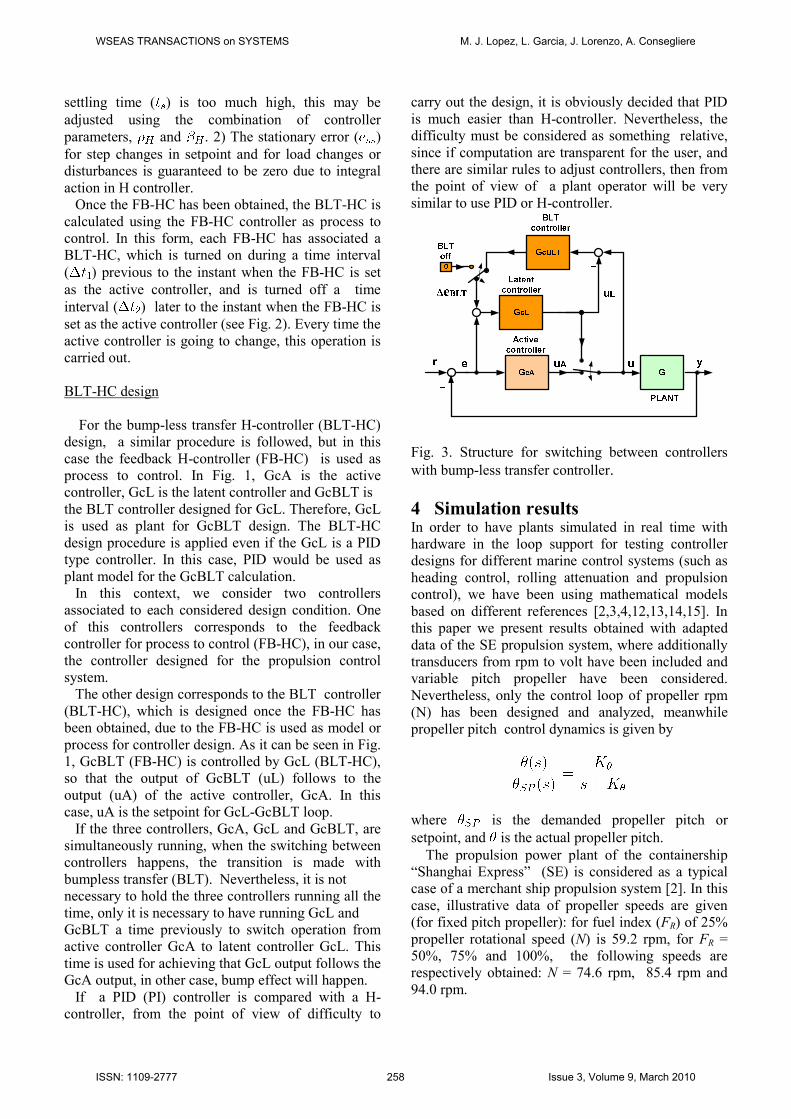
process to control. In Fig. 1, GcA is the active

controller, GcL is the latent controller and GcBLT is

the BLT controller designed for GcL. Therefore, GcL

is used as plant for GcBLT design. The BLT-HC

design procedure is applied even if the GcL is a PID

type controller. In this case, PID would be used as

plant model for the GcBLT calculation.

In this context, we consider two controllers

associated to each considered design condition. One

of this controllers corresponds to the feedback

controller for process to control (FB-HC), in our case,

the controller designed for the propulsion control

system.

The other design corresponds to the BLT controller

(BLT-HC), which is designed once the FB-HC has

been obtained, due to the FB-HC is used as model or

process for controller design. As it can be seen in Fig.

1, GcBLT (FB-HC) is controlled by GcL (BLT-HC),

so that the output of GcBLT (uL) follows to the

output (uA) of the active controller, GcA. In this

case, uA is the setpoint for GcL-GcBLT loop.

If the three controllers, GcA, GcL and GcBLT, are

simultaneously running, when the switching between

controllers happens, the transition is made with

bumpless transfer (BLT). Nevertheless, it is not

necessary to hold the three controllers running all the

time, only it is necessary to have running GcL and

GcBLT a time previously to switch operation from

active controller GcA to latent controller GcL. This

time is used for achieving that GcL output follows the

GcA output, in other case, bump effect will happen.

If a PID (PI) controller is compared with a H-

controller, from the point of view of difficulty to

carry out the design, it is obviously decided that PID

is much easier than H-controller. Nevertheless, the

difficulty must be considered as something relative,

since if computation are transparent for the user, and

there are similar rules to adjust controllers, then from

the point of view of a plant operator will be very

similar to use PID or H-controller.

Fig. 3. Structure for switching between controllers

with bump-less transfer controller.

4 Simulation results In order to have plants simulated in real time with

hardware in the loop support for testing controller

designs for different marine control systems (such as

heading control, rolling attenuation and propulsion

control), we have been using mathematical models

based on different references [2,3,4,12,13,14,15]. In

this paper we present results obtained with adapted

data of the SE propulsion system, where additionally

transducers from rpm to volt have been included and

variable pitch propeller have been considered.

Nevertheless, only the control loop of propeller rpm

(N) has been designed and analyzed, meanwhile

propeller pitch control dynamics is given by

where is the demanded propeller pitch or

setpoint, and is the actual propeller pitch.

The propulsion power plant of the containership

“Shanghai Express” (SE) is considered as a typical

case of a merchant ship propulsion system [2]. In this

case, illustrative data of propeller speeds are given

(for fixed pitch propeller): for fuel index (FR) of 25%

propeller rotational speed (N) is 59.2 rpm, for FR =

50%, 75% and 100%, the following speeds are

respectively obtained: N = 74.6 rpm, 85.4 rpm and

94.0 rpm.



For a given plant condition, the linearized model

has the following form:

For nominal operation (FR = 75% and N = 85.4

rpm, Kg = 1) is given by

G(s) relates rpm of the ship propeller expressed in

volts (output of rpm transducer) with the controller

signal in volts (input to injection actuator). This

response is used for system identification and the

following estimated model (first order plus dead time,

FOPDT) is obtained. This model is used in practice

for PID tuning.

FOPDT and linearized models are used for

controller design, and the obtained results with PID

and controller are analyzed with the nonlinear

model described before. For controller design, dead

time term is approximated as a first order Padé

approximation. Advantages of controller are

basically: 1) easy to design using our procedure

implemented in ControlAvH software [21,22], b) our

fine tuning procedure only depends on two

parameters ( ) and it is based on basic rules, c)

control system performance and robustness are

improved with respect to PID. Classical drawbacks

associated with control, such as difficult of the

design procedure and high order or the controller are

overcome. On one hand, this is due to the fact that a

digital fourth/fifth order controller is easy to

implement in hard real time for specific digital

processors (such as microcontrollers or digital signal

processors, DSP), for Programmable Automation

Controller (PAC) such as the provided by NI [23] and

also for an industrial programmable automata or PLC

(in case of recursive algorithms or difference

equations can be implemented in the software of the

respective PLC of new generation); and for the other

side, the design procedure is transparent for the user,

due to he only must take into account the relation

between two design parameters ( ) and its

relation with the control system observed response.

No theoretical knowledge about control is

needed for controller fine tuning.

In Fig. 4, closed-loop system responses for three

operation conditions (nominal and two others with

±50% changes in stationary gain for the plant) and a

fixed H-controller (designed for Kg=1) are shown.

These conditions corresponds to changes in stationary

gain characterized by Kg parameter, which takes

three values: Kg = 1, 1.5 and 0.5. Nevertheless, as it

can be seen, one response is so slow (for Kg = 0.5),

and other has excessive overshoot (for Kg = 1.5).

Therefore, three controllers (Gc1, Gc2 and Gc3) must

be designed, one for each plant operation condition.

In this case, satisfactory responses (extremely similar

behavior) are also obtained for Kg = 0.5 and for Kg =

1.5. The used parameters for the three FB-HC designs

are the following:

0 1 2 3 4 5 6 7 80

0.2

0.4

0.6

0.8

1

1.2

Time (sec)

∆∆ ∆∆ N

(vo

lt)

Fig. 4. Closed-loop system responses for three

operation conditions (Kg = 1, 1.5, 0.5) and a fixed H-

controller designed for Kg = 1.

0 0.5 1 1.5 2 2.5 30

0.5

1

Time (sec)

∆∆ ∆∆ R

PM

(vo

lt)

0 0.5 1 1.5 2 2.5 30

0.5

1

Time (sec)

∆∆ ∆∆ C

O (

volt

)

Fig. 5. Closed-loop system responses for three

operation conditions (Kg = 1, 1.5, 0.5) with their

respective H-controllers.

In Fig. 5, the closed-loop system responses for

three operation conditions (Kg = 1, 1.5, 0.5) and their

respective H-controllers (designed for each operation

condition) are shown. Practically the same RPM

responses are obtained for the three controllers. Due

to the proximity between the three RPM responses, it

seems that only one curve appears in this Figure.

In order to prove BLT controller the following

tests are considered:



Test 1. System is in stationary state with controller

designed for Kg = 1 (Gc1 as active controller GcA),

and it is decided to switch to controller designed for

Kg = 0.5 (Gc3 as latent controller GcL). If BLT

controller is not used, the bump effect happens as it is

shown in Figure 6. If BLT is considered, BLT

controller can be activated in different instants: a)

when it is decided to change the controller from Gc1

to Gc3, b) one half second before to controller

switching. If case a) is considered, BLT controller

needs a settling time to reduce differences between

uL and u (see Figure 3), and therefore bump effect

will not be avoid completely. If case b) is tested, the

previous time is used to get that (uL-u) be sufficiently

small and bump-less controller switching is obtained.

The following parameters have been used for BLT

controller (GcBLT in Figure 3):

Test 2. In this case, the controller Gc3 (designed for

Kg = 0.5) is used as plant to control, and the GcBLT

is its controller.

0 1 2 3 4 5 6 7 8

0

0.5

1

1.5

Time (sec)

∆∆ ∆∆ R

PM

(vo

lt)

0 1 2 3 4 5 6 7 80

2

4

Time (sec)

∆∆ ∆∆ C

O (

volt

)

Fig. 6. Closed-loop response for controller switching

(Gc1 to Gc3) at t = 3 sec., without BLT controller.

Without BLT controller, bump effect is significant

as it can be seen in Fig. 6. Resultant effect from

switching is an equivalent disturbance. For that, it is

employed the BLT controller. In Fig. 5 it can be

shown behavior when a BLT (Gc_BLT for Gc3) is

used. In this case, controller for BLT (Gc_BLT) is

connected 0.5 sec. before controller switching. This

time is necessary for controller convergence: uL � u,

where u is the actual control signal (from the active

controller) and uL is the signal generated by the latent

controller (see Fig. 3).

Hard real time control and simulation

In our laboratory, a Hard Real Time Control and

Simulation Environment (EPESC) [9,10] has been

developed, for PC-based controllers and PC-based

plant simulators; due to PC-based environments are

cheaper than industrial-grade processors and have a

more open architecture. This open architecture means

0 1 2 3 4 5 6 7 8

0

0.5

1

1.5

Time (sec)

∆∆ ∆∆ R

PM

(vo

lt)

0 1 2 3 4 5 6 7 80

2

4

Time (sec)

∆∆ ∆∆ C

O (

volt

)

Fig. 7. Bumpless transfer switching from controller

Gc1 to controller Gc3 in t = 3 sec.

that third-party vendor is able to supply more of the

components. Communication between PCs is based

on the Ethernet hardware. Low-cost communication

suggested the use of TCP/IP or UDP/IP, which are

nonproprietary communication protocols. The

TCP/IP protocols guarantees, via implicit

acknowledgment, receipt of data packets, but

occupies a wider network bandwidth. The UDP/IP

protocol is faster, but does not guarantee absence of

packet losses. Basically, the communication between

PC1 and PC2 consists of controller matrices, tuning

parameters and data for controller analysis and fine

tuning. For that, we have adopted the TCP/IP

protocol.

The essence of real-time systems is that they are

able to respond to external stimuli within a certain

predictable period of time. Building real time

computing systems is challenging due to

requirements for reliability and efficient, as well as

for predictability in the interaction among

components. Real-time operating systems (RTOS)

such as VxWorks, QNX and LynxOS [26, 27, 28]

facilitate real-time behavior by scheduling processes

to meet the timing constraints imposed by the

application. Control systems are among the most

demanding of real-time applications. There are

constraints on the allowable time delays in the

feedback loop (due to latency and jitter in

computation and in communication), as well as the

speed of response to an external input such as

changing environmental conditions or detected

faulted conditions. If the timing constraints are not

met, the system may become unstable.

EPESC system consists of hardware (input/output

interface and electronic card for data acquisition) and

a software application developed with C/C++

language, Linux Operating System and RTAI (Real

Time Application Interface for Linux) [25]. RTAI

lets to develop applications with strict timing

constraints, but has the difference with respect to



other real time operating systems (QNX, VxWorks,

and LynxOS) that, like Linux itself, this software is a

community effort and freeware. RTAI supports

several architectures, such as X86/Pentium or

PowerPC. EPESC is used for hard real time controller

implementation and for process simulator, both

implemented with PC (see Fig. 8).

Fig. 8. Hard real time simulation environment

(EPESC)

Both devices, the controller and the plant

simulator, with their respective applications must be

able to transmit and to acquire signals on a hardware

communication channel. In order to make any

application unaware of the presence of hardware or

software on the other side of the control loop it has

been decided to implement COMEDI drivers [24] for

communications boards. The COMEDI package has

been chosen because it is an open-source product

widely used in the field of automation. Indeed

COMEDI provides a standard for drivers of DAQ

(Digital Acquisition boards) under Linux.

A COMEDI driver for National Instrument (NI) PCI-

6014 [21] boards has been used. Two boards are use

for the plant simulator (PLANT) and other two for

the controller (CONTROLLER).

In order to reach the central idea of the EPESC

system, to evaluate the control systems, taking into

account the hardware in the loop, input and output

electrical signals are present, such as: the

CONTROLLER signals (input process variable, PV,

controller output, CO), and the PLANT signals

(output process variable, PV, manipulate variable,

(MV) are both wired signal interconnecting by means

of two multi I/O data acquisition cards. These cards

provide the electric input-output signals among them,

and realistic simulations are carried out.

The simulated plant is implemented by means of a

RT-thread, the so-called PLANT. This task executes

the following algorithm:

1) Load the plant mathematical model.

2) Set the initial state for plant variables.

3) While not end simulation, do:

4) Read input data from COMEDI device.

5) Convert voltage magnitude to physic variable.

6) Compute the plant states and outputs.

7) Send via FIFO the relevant data to DISPLAY

Linux process.

8) Convert physic magnitude to equivalent voltage.

9) Suspend the task to wait period.

10) Write output data to COMEDI device.

11) Go to step 3).

The three digital controllers (active controller,

latent controller and bumpless transfer controller) are

implemented by means of a RT-thread, the so-called

CONTROLLER. This task executes the following

algorithm:

1) Set the initial state for controllers variables.

2) Expect the reception of controllers parameters.

3) While not stop requested:

4) Read input data from COMEDI device.

5) Convert voltage magnitude to physic variable.

6) Compute error signal for GcA (active controller)

e(k) = SP(k) – PV(k)

7) Compute controller output error between GcA

and GcL, eu(k) = uA(k) – uL(k),

8) Compute discrete state space controllers

algorithms for GcA, GcBLT and GcL:

Gca (active controller):

GcBLT (bumpless transfer controller):

GcL (latent controller):

9) Send via FIFO the relevant data to DISPLAY.

10) Convert physic magnitude to equivalent voltage.

11) Suspend the task to wait period.

12) Write output data to COMEDI device.

13) Go to step 3).

Active controller (GcA) and latent controller (GcL)

with its BLT controller (GcBLT) must be executed

on-line. This implies higher computational load, but it

is guaranteed that BLT is achieved. Nevertheless, it is

not necessary to hold the three controllers running all

the time, only it is necessary to have running GcL and

GcBLT a time previously to switch operation from

active controller GcA to latent controller GcL. This

time is used for achieving that the GcL output follows

PC2: CONTROLLERPC1: SIMULATOR

TAD: 2 NI PCI-6014 TAD: 2 NI PCI-6014

Connection Panel

- Linx-RTAI- Data acquisition cards I/O (TAD). - Interface Connection Pannel (ICP).- Simulator: PC1 + TAD + ICP- Controller PC2 + TAD + ICP

PC2: CONTROLLERPC1: SIMULATOR

TAD: 2 NI PCI-6014 TAD: 2 NI PCI-6014

Connection Panel

- Linx-RTAI- Data acquisition cards I/O (TAD). - Interface Connection Pannel (ICP).- Simulator: PC1 + TAD + ICP- Controller PC2 + TAD + ICP



the GcA output, in other case, bump effect will

happen.

6 Conclusions A method for H∞ controller design and switching

between controllers without bump effect has been

proposed, and it has been applied to a simulated

marine propulsion system, with diesel engine used as

propeller prime-mover.

Each design consists of a feedback H-controller

(FB-HC) and a bump-less transfer H-controller

(BLT-HC). The method is implemented in an auto-

tuning procedure by means ControlAvH [21,22].

Satisfactory results are obtained using hardware in

the loop simulations (HILS) with EPESC [9,10]. The

employment of our method gives good performance

and robustness properties, and bump-less transfer

when switching between controllers are carried out.

In next works, experimental marine systems will

employ to test our design methodology in

collaboration with a marine construction company.

References:

[1] Rakopoulos C. D., E. G. Giakoumis (2009).

Diesel Engine Transient Operation. Principles of

Operation and Simulation Análisis. Springer.

[2] Xiros N. (2002). Robust Control of Diesel Ship

Propulsion. Springer.

[3] Izadi-Zamanabadi R., M. Blanke (1999). A ship

propulsion system as a benchmark for fault-

tolerant control. Control Engineering Practice 7,

pp 227-239.

[4] Fossen T. I. (2002). Marine Control Systems.

Marine Cybernetics.

[5] Altosole M., G. Benvenuto, M. Figari, U.

Campora (2009). Real-time simulation of a

COGAG naval ship propulsión system. Proc.

IMechE vol. 223 Part M: J. Engineering for the

Maritime Environment.

[6] Campora U., M. Figari (2003). Numerical

simulation of ship propulsion transients and full-

scale validation. Proc. IMechE vol. 217 Part M: J.

Engineering for the Maritime Environment.

[7] Samad T., G. Balas (Ed.) (2003). Software-

Enabled Control. IEEE Press.

[8] Gazi V., M. L. Moore, K. M. Pasión, W. P.

Shackleford, F. M. Proctor, J. S. Albus (2001).

The RCS Handbook. Tools for real-time control

systems software development. Wiley.

[9] Garcia L., M. J. Lopez, J. Lorenzo (2006). Hard

Real Time Based on Linux/RTAI for Plant

Simulation and Control Systems

Evaluation.WSEAS Transactions on Systems and

Control, Vol. 1, Issue 2, pp 161-168.

[10] Garcia L., M. J. Lopez, J. Lorenzo (2006).

Hardware in the loop Environment for Control

System Evaluation under Linux/RTAI.

Proceedings of the 6th WSEAS International

Conference on Applied Computer Science,

Tenerife (Spain), pp 285-290.

[11] Roy S., O. P. Malik, G. S. Hope (1991). An

adaptive control scheme for speed control of

diesel driven power-plants. IEEE Transactions on

Energy Conversion, Vol. 6, No. 4, pp 605-611.

[12] Banning R., M. A. Johnson, M. J. Grimble

(1997). Advanced Control Design for Marine

Diesel Engine Propulsion Systems. Journal of

Dynamic Systems, Measurement and Control,

Vol. 119, pp 167-174.

[13] Kallstrom C. G., P. Ottosson (1982). The

generation and control of roll motion of ships in

close turns. Fourth International Symposium on

Ship Operation Automation, Genova.

[14] Lewis E. V. (1989). Principles of Naval

Architecture, SNAME.

[15] Amerongen J. van, P. G. M. van der Klugt, H.

R. van Nauta Lemke (1990). Rudder Roll

Stabilisation for Ships. Automatica, Vol. 26, No.

4, pp. 679-690.

[16] Skogestad S., I. Postlethwaite (2003).

Multivariable Feedback Control. Analisis and

Design. Wiley.

[17] Grimble M. J. (2001). Industrial Control

Systems Design. Wiley.

[18] Zhou K., J. C. Doyle, K. Glover (1996). Robust

and Optimal Control. Prentice Hall.

[19] O’Dwyer (2006). Handbook of PI and PID

Controller Tuning Rules. Imperial College Press.

[20] Matlab and Simulink. © Mathworks.

[21] Lorenzo J., M. J. Lopez, L. Garcia (2006). H2

and H∞ controllers design methodology using

ControlAvH software for SISO and MIMO

processes control. WSEAS Transactions on

Systems. Issue 11, Vol. 4, pp 1829-1837.

[22] Lorenzo J., M. J. Lopez, L. Garcia (2006).

Flexible Software and Strict Real Time System for

H∞ Controller Design, Hardware Implementation

and Plant Simulation. WSEAS Transactions on

Computers. Issue 7, Vol. 5, pp 1413-1420.

[23] National Instruments Corporation. Measurement

and automation catalog. http://www.ni.com.

[24] COMEDI –The Linux Control and Measurement

Device Interface. http://www.comedi.org/

[25] RTAI. http://www.aero.polimi.it/rtai.

[26] LynxOS RTOS. http://www.lynuxworks.com.

[27] QNX Software Systems. http://www.qnx.com.

[28] VxWorks RTOS. http://www.windriver.com.



design methodology based on h∞ control theory for marine ... · marine propulsion system with...

Documents