design guidelines for frp honeycomb sandwich bridge decks
TRANSCRIPT

Graduate Theses, Dissertations, and Problem Reports
2008
Design guidelines for FRP honeycomb sandwich bridge decks Design guidelines for FRP honeycomb sandwich bridge decks
Bin Zou West Virginia University
Follow this and additional works at: https://researchrepository.wvu.edu/etd
Recommended Citation Recommended Citation Zou, Bin, "Design guidelines for FRP honeycomb sandwich bridge decks" (2008). Graduate Theses, Dissertations, and Problem Reports. 2869. https://researchrepository.wvu.edu/etd/2869
This Dissertation is protected by copyright and/or related rights. It has been brought to you by the The Research Repository @ WVU with permission from the rights-holder(s). You are free to use this Dissertation in any way that is permitted by the copyright and related rights legislation that applies to your use. For other uses you must obtain permission from the rights-holder(s) directly, unless additional rights are indicated by a Creative Commons license in the record and/ or on the work itself. This Dissertation has been accepted for inclusion in WVU Graduate Theses, Dissertations, and Problem Reports collection by an authorized administrator of The Research Repository @ WVU. For more information, please contact [email protected].

DESIGN GUIDELINES FOR FRP HONEYCOMB
SANDWICH BRIDGE DECKS
By
Bin Zou
Dissertation submitted to the
College of Engineering and Mineral Resources at West Virginia University
in partial fulfillment of the requirements for the degree of
Doctor of Philosophy
in Civil Engineering
Julio F. Davalos, Ph.D., Chair
Karl E. Barth, Ph.D., Co-Chair An Chen, Ph.D.
Kenneth H. Means, Ph.D. Jacky C. Prucz, Ph.D.
Indrajit Ray, Ph.D.
Department of Civil and Environmental Engineering
Morgantown, West Virginia 2008
Keywords: Fiber-reinforced polymer (FRP), bridge decks, shear connection, load
distribution, composite action, effective width
Copyright © 2008 Bin Zou
DESIGN GUIDELINES FOR FRP HONEYCOMB
SANDIWICH BRIDGE DECKS
Bin Zou
Advisor: Dr. Julio F. Davalos Abstract: Fiber-Reinforced Polymer (FRP) Bridge decks offer great advantages in highway bridge rehabilitation and new construction, due to reduced weight and maintenance costs, and enhanced durability and service-life. In practice, however, lack of bridge engineering design standards and guidelines have prevented wider acceptance and application of FRP bridge decks by transportation officials. This dissertation focuses on the study of an engineered FRP deck-steel stringer bridge system through experimental testing and both Finite Element analyses and analytical methods. A prototype mechanical shear connection was developed and designed to be used with any type of FRP panels that can accommodate any panel heights. This non-grouted sleeve-type connector can secure the deck onto a welded stud and can sustain shear forces at FRP panel- steel stringer interface. Static and fatigue tests were conducted on push-out connection specimens, and later on a scaled bridge model. The strength, stiffness, and fatigue performance characteristics of the connection were fully investigated. Constructability issues were also evaluated, such as ease of installation and economic manufacturing of the connector. Design formulations were established based on the test results. Following the connection study, a 1:3 scaled bridge model of a honeycomb FRP deck on steel stringers was evaluated. The deck was attached to three supporting steel stringers using the proposed sleeve-type mechanical connections. The model was designed as partially composite to satisfy AASHTO limits and requirements. Several issues were evaluated that included: (1) deck attachment procedures; (2) transverse load distribution factors; (3) local deck deflections; and (4) system fatigue behavior. After the bridge model was tested in the linear range, a 1.2-m wide T-section, of an FRP deck section attached to the middle stringer, was cutout from the bridge model and tested in bending for service and failure loads. The evaluations included: (1) Degree of composite action, (2) Effective deck-width, and (3) service-limit and ultimate-limit states under flexure loads. The behavior of the FRP deck under partial composite action was defined fully by these tests.

Finite element models of the scaled bridge model and T-beam section were formulated using ABAQUS. Besides the experimental tests and FE analyses, analytical solutions were developed to verify the test results. An explicit series solution for stiffened orthotropic plates was used to evaluate the bridge response and obtain load distribution factors of FRP deck-on-steel-stringer bridges. Also a harmonic analysis that was developed for FRP thin-walled sections was formulated to define effective-width for FRP decks as an explicit solution. The outcome of this study was to propose design guidelines and recommendations for FRP honeycomb bridge decks for applications in bridge engineering practice.

iv
ACKNOWLEDGEMENTS
I would like to express my gratitude to my advisor and committee chair, Dr. Julio F.
Davalos, for his continuing assistance, support, guidance, understanding and
encouragement throughout my graduate studies. I am also thankful to my committee co-
chair, Dr. Karl E. Barth, for the guidance and support he has offered, both on this project
and in other aspects.
I would like to thank Dr. An Chen, Dr. Kenneth H. Means, Dr. Jacky C. Prucz, and Dr.
Indrajit Ray for their participation in my advisory committee. The laboratory assistance
of William J. Comstock is greatly appreciated. I would also like to thank Dr. Jerry D.
Plunkett and KSCI for providing the experimental test samples; Their support is greatly
appreciated. I also must thank my parents and family for their everlasting support and
blessings in my life.

v
TABLE OF CONTENTS
ABSTRACT………………………………………………………………..ii
ACKNOWLEDGEMENTS……………………………………………….iv
TABLE OF CONTENTS………………………………………………….v
LIST OF FIGURES……………………………………………………….ix
LIST OF TABLES……………………………………………………….xiii
CHAPTER 1 INTRODUCTION………………………………………...1
1.1 Overview of FRP Decks Applications in Bridge Engineering……………………1 1.2. Problem Statement and Research Significance…………………………………...3 1.3. Objectives and Scope……………………………………………………………..6 1.4. Organization………………………………………………………………………7
CHAPTER 2 A NEW SHEAR CONNECTION FOR FRP BRIDGE
DECKS…………………………………………………………………….10 2.1. Introduction……………………………………………………………………...10 2.2. Background and Problem Statement…………………………………………….11
2.2.1. Existing Shear Connections for FRP Decks ……………………………...12 2.2.2. Shear Connections for Concrete Composite Deck………………………...15 2.2.3. Fatigue Resistance of Shear Connection…………………………………..18 2.2.4. Experimental Methods on Shear Connections…………………………….19 2.2.5. Problem Statement………………………………………………………...20
2.3. Objectives and Scope……………………………………………………………21 2.4. Prototype Shear Connection and Test Procedure………………………………..21
2.4.1. Prototype Shear Connection ……………………………………………...22 2.4.2. Push-out Specimen and Test Setup……………………………………….27 2.4.3. Test Procedure…………………………………………………………….28 2.4.4. Fatigue Test on a Scaled Bridge Model…………………………………..30
2.5. Test Results and Design Formulation…………………………………………...32 2.5.1. Static Strength and Load Displacement Formulation ( ∆−P Curve) ……32 2.5.2. Fatigue Strength and S-N Curve…………………………………………..37 2.5.3. Fatigue Resistance of Connection in Bridge Model………………………39
2.6. Conclusions……………………………………………………………………...40

vi
CHAPTER 3 EXPERIMENTAL STUDY ON REDUCED SCALE
FRP BRIDGE MODEL…………………………………………………..42
3.1. Introduction……………………………………………………………………..42 3.2. Background and Problem Statement……………………………………………43
3.2.1. Load Distribution Factor………………………………………………….44 3.2.2. Effective Flange Width……………………………………………………52 3.2.3. Degree of Composite Action……………………………………………...60 3.2.4. Current Development and Application of FRP Deck Bridges……………60 3.2.5. Problem Statement………………………………………………………...62
3.3. Objectives and Scope……………………………………………………………63 3.4. Scaled FRP Bridge Model………………………………………………………64
3.4.1. Bridge Model Description…………………………………………………65 3.4.2. T-section Model Description………………………………………….......70
3.5. Test Procedure…………………………………………………………………..70 3.5.1. Phase I Test………………………………………………………………..71 3.5.2. Phase II Test……………………………………………………………….74 3.5.3. Phase III Test……………………………………………………………...74
3.6. Test Results……………………………………………………………………...76 3.6.1. Load Distribution Factors…………………………………………………76 3.6.2. Local Deck Deflection…………………………………………………….77 3.6.3. Degree of Composite Action……………………………………………...78 3.6.4. Effective Flange Width……………………………………………………79 3.6.5. Failure Mode at Strength Limit……………………………………………81 3.6.6. Fatigue Resistance………………………………………………………...82
3.7. Conclusions and Summaries…………………………………………………….83 APPENDIX A: DESIGN OF A FRP SLAB-STEEL STRINGER BRIDGE………..86
CHAPTER 4 FE ANALYSIS OF SCALED BRIDGE AND T-
SECTION MODEL……………………………………………………….92
4.1. Introduction……………………………………………………………………...92 4.2. FE Model description……………………………………………………………92
4.2.1. FRP Panel and Equivalent Properties……………………………………..93 4.2.2. Steel Stringer………………………………………………………………96 4.2.3. Shear Connections………………………………………………………...96
4.3. FE Analysis Results……………………………………………………………..98 4.3.1. Load Distribution Factor…………………………………………………..98 4.3.2. Local Panel Deflection…………………………………………………….99

vii
4.3.3. Effective Flange Width…………………………………………………..100 4.4. Summary……………………………………………………………………….102 APPENDIX B: FRP Panel Properties Evaluation………………………………….103
CHAPTER 5 EVALUATION OF LOAD DISTRIBUTION FACTOR
BY SERIES SOLUTION………………………………………………..109
5.1. Introduction…………………………………………………………………….109 5.2. Objectives and Scope…………………………………………………………..110 5.3. Series Solution for Stiffened Plate……………………………………………..110
5.3.1. Series Solution for Stiffened Plate under Symmetric Load……………...111 5.3.2. Series Solution for Stiffened Plate under Anti-symmetric Load………...118 5.3.3. Series Solution for Stiffened Plate under Asymmetric Load…………….119 5.3.4. Load Distribution Factors by Series Solution……………………………120
5.4. Parametric Study on Load Distribution Factors………………………………..120 5.4.1. FE Model Descriptions…………………………………………………..123 5.4.2. Live Load Position……………………………………………………….126 5.4.3. Load Distribution Factor and FE Results………………………………...126 5.4.4. Assessment and Discussion of FE Results and Series Solution…………126
5.4.4.1. Girder Spacing……………………………………………………..128 5.4.4.2. Span Length………………………………………………………..128 5.4.4.3. Number of Lane Loaded…………………………………………...131 5.4.4.4. Cross Section Stiffness…………………………………………….132
5.4.5. Comparison of Distribution Factor from Series Solution Formulation and FE Analysis……………………………………………………………….132
5.4.6. Application of Series Solution to FRP Deck…………………………….134 5.4.7. Regression Function for Distribution Factor…………………………….135
5.5. Summary and Conclusion……………………………………………………...137
CHAPTER 6 EFFECTIVE FLANGE WIDTH OF FRP BRIDGE
DECKS…………………………………………………………………...138
6.1. Introduction…………………………………………………………………….138 6.2. Objectives and Scope…………………………………………………………..140 6.3. Shear Lag Model……………………………………………………………….140 6.4. Parametric Study on Effective Flange Width………………………………….146
6.4.1. FE Model Descriptions…………………………………………………..146 6.4.2. Live Load Position……………………………………………………….148 6.4.3. Effective Flange Width Data Reduction from FE Results……………….148 6.4.4. Assessment and Discussion of FE Results and Analytical Solution……..149

viii
6.4.4.1. Number of Lanes Loaded…………………………………………..150 6.4.4.2. Flange Thickness…………………………………………………..151
6.4.4.3. Aspect Ratio………………………………………………………..152 6.4.4.4. In-plane Extensional Modulus/Shear Modulus Ratio……………...152 6.4.5. Comparison between Shear Lag Model and FE Analysis……………….155 6.4.6. Comparison between Shear Lag Model and Empirical Function………..155 6.4.7. Application of Shear Lag Model to FRP Deck…………………………..160
6.5. Conclusions…………………………………………………………………….160
CHAPTER 7 CONCLUSIONS AND DESIGN
RECOMMENDATIONS………………………………………………..162
7.1. Conclusions…………………………………………………………………….162 7.1.1. Overview…………………………………………………………………162 7.1.2. Effective Prototype Shear Connection…………………………………...163 7.1.3. Load Distribution Factor…………………………………………………164 7.1.4. Panel Local Deflection…………………………………………………...165 7.1.5. Degree of Composite Action and Effective Flange Width………………165 7.1.6. Shear Connection Spacing……………………………………………….166 7.1.7. Service Load and Failure Mode………………………………………….166
7.2. Summaries……………………………………………………………………...167 7.3. FRP Deck Bridge Design Recommendations and Flow Chart………………...168 7.4. Future Works…………………………………………………………………..169
REFERENCES…………………………………………………………..170

ix
LIST OF FIGURES
Figure 1.1 Typical Cellular FRP Panels………………………………………………...2
Figure 1.2 KSCI Honeycomb FRP Panel……………………………………………….3
Figure 2.1 Force Equilibrium and Strain Compatibility of Deck-Stringer…………16
Figure 2.2 Full Composite Action vs. Non-composite Action Beams………………..17
Figure 2.3 KSCI Honeycomb Sandwich Panel………………………………………..20
Figure 2.4 Prototype Shear Connections……………………………………………...22
Figure 2.5 Installations of Shear Connection to FRP Decks ………………………...23
Figure 2.6 Shear Connection Test Setup………………………………………………28
Figure 2.7 Shear Connection Test Setup ……………………………………………...28
Figure 2.8 Scaled Bridge Model ……………………………………………………….31
Figure 2.9 Deformation to Outside and Inside Washer of Top Steel Sleeve………..33
Figure 2.10 Deformation to Bottom Sleeve……………………………………………34
Figure 2.11 Bottom Facesheet at Yield………………………………………………..34
Figure 2.12 Bottom Facesheet at Failure……………………………………………...34
Figure 2.13 Loads and Displacements Data (Specimens S2-S8) …………………….35
Figure 2.14 Segmental Linear Load Displacement Curve…………………………...37
Figure 2.15 Fracture of Shear Stud……………………………………………………38
Figure 2.16 Delamination of Bottom Facesheet………………………………………38
Figure 2.17 NS − Curve of Shear Connection………………………………………38
Figure 2.18 Bridge Stiffness Variations during Fatigue Test………………………..39
Figure 3.1 Effective Flange Width Definition…………………………………………53
Figure 3.2 KSCI honeycomb FRP panel………………………………………………65
Figure 3.3 Scaled bridge model………………………………………………………..66
Figure 3.4 Tongue-and-groove connections…………………………………………...67
Figure 3.5 Tongue and Groove Connection with FRP Sheet Covered………………67
Figure 3.6 Installations of Shear Connection to FRP Decks…………………………67
Figure 3.7 Plan View of Bridge Model………………………………………………...69
Figure 3.8 Elevation View of Bridge Model…………………………………………...69
Figure 3.9 Cross Section of Bridge Model ……………………………………………69

x
Figure 3.10 Cross Section of Test Model……………………………………………...70
Figure 3.11 Bridge model test …………………………………………………………71
Figure 3.12 Instrumentation of bridge model………………………………………...72
Figure 3.13 Local deflection definitions……………………………………………….73
Figure 3.14 Instrumentation of T-beam FRP deck section…………………………..75
Figure 3.15 Instrumentation of T-beam Girder………………………………………76
Figure 3.16 Deflection Profile………………………………………………………….79
Figure 3.17 Neutral Axis Position for Load Case 1 and 2……………………………79
Figure 3.18 Normal Strain Distribution on Top Facesheet of FRP Panel…………..80
Figure 3.19 Normal Strain Distribution on Bottom Facesheet of FRP Panel………80
Figure 3.20 Stress Integration of the Flange………………………………………….81
Figure 3.21 Axial Strain Distribution at Mid-span Section (Load Case 1) ………...81
Figure 3.22 T-section at Failure……………………………………………………….82
Figure 3.23 Load Deflection Curve for Load Case 2 at Mid-span…………………..82
Figure 3.24 Stiffness Ratio Variations during Fatigue Test…………………………83
Figure 4.1 Facesheet Lay-up…………………………………………………………...94
Figure 4.2 Illustration of Connector Element………………………………………...97
Figure 4.3 FE Bridge Model……………………………………………………………97
Figure 4.4 Deformed Shape of Panel…………………………………………………..99
Figure 4.5 Deflection Profile of FRP Panel…………………………………………..100
Figure 4.6 Stress Integration of the Flange………………………………………….101
Figure 5.1 Two-side Stiffened Orthotropic Plate with Equally Spaced
Stringers..........................................................................................................................112
Figure 5.2 Two-side Stiffened Orthotropic Plate with Exterior Stringers
Only…………………………………………………………………………………….113
Figure 5.3 Typical Interior Stringer………………………………………………….113
Figure 5.4 Typical Cross Section of Bridge Model………………………………….122
Figure 5.5 Configuration of Finite Elements………………………………………...123
Figure 5.6 AASHTO HS20 Truck Load for 1-, 2-, and 3- lane Loaded Case……...124
Figure 5.7 AASHTO HS20 Truck Load Longitudinal Position……………………124

xi
Figure 5.8 Critical Transverse Position for Three-lane Bridge CS4 with 30.5m Span
length (One Lane Loaded) ………………………………………………………….125
Figure 5.9 Influence of Girder Spacing for interior girder with three lanes bridges
(bridge spans 15.2m and 30.5m) ……………………………………………………127
Figure 5.10 Influence of Girder Spacing for exterior girder with three lanes bridges
(bridge spans 15.2m and 30.5m) …………………………………………………….127
Figure 5.11 Influence of Span Length on Distribution Factor for Interior Girder
with Two-lane Loaded (Cross Section CS4) ………………………………………..129
Figure 5.12 Influence of Span Length on Distribution Factor for Exterior Girder
with Two-lane Loaded (Cross Section CS4) ………………………………………..129
Figure 5.13 Influence of Number of Lanes Loaded on Distribution Factor for
Interior Girder (Cross Section CS4) ………………………………………………...131
Figure 5.14 Influence of Number of Lanes Loaded on Distribution Factor for
Exterior Girder (Cross Section CS4) ………………………………………………..131
Figure 5.15 Influence of Composite Section Moment of Inertia on Distribution
Factors………………………………………………………………………………….132
Figure 6.1 Typical Panel Element with Two Sides Stiffened……………………….140
Figure 6.2 Shear flow in Flange Element…………………………………………….141
Figure 6.3 Isolated Panel Elements…………………………………………………..142
Figure 6.4 Effective Flange Width……………………………………………………145
Figure 6.5 Typical Cross Section of Bridge Model………………………………….147
Figure 6.6 AASHTO HS20 Truck Live Load………………………………………..148
Figure 6.7 Stress Integration along the Flange Width………………………………149
Figure 6.8 Comparison of Number of Lane Loaded for Bridge Section CS1……..151
Figure 6.9 Comparison of Number of Lane Loaded for Bridge Section CS4……..151
Figure 6.10 Aspect Ratio vs. Effective Width……………………………………….154
Figure 6.11 Effective Width of FRP Panel vs. Concrete Panel for Bridge Section
CS1 …………………………………………………………………………………….154
Figure 6.12 Comparison of Shear Lag Model and FE for Bridge Section
CS4……………………………………………………………………………………..156

xii
Figure 6.13 Comparison between Shear Lag Model and Empirical Function for
10/ =GE ………………………………………………………………………………158

xiii
LIST OF TABLES
Table 2.1 Fatigue Test Results…………………………………………………………30
Table 2.2 Static Strength of Shear Connections………………………………………35
Table 3.1 Load Case Designation……………………………………………………...73
Table 3.2 Load Distribution Factor of Test Model…………………………………..77
Table 3.3 Deflection Profile of Test Model……………………………………………78
Table 3.4 Stiffness Ratio of Bridge Model during Fatigue Test……………………..83
Table 4.1 Material Properties of Facesheet…………………………………………...95
Table 4.2 Stiffness Properties of Facesheet Lamina………………………………….95
Table 4.3 Stiffness Properties of Facesheet and Core………………………………..95
Table 4.4 Equivalent Properties of FRP Panel……………………………………….95
Table 4.5 Load Distribution Factor of Bridge Model………………………………..99
Table 4.6 Deflection Profile of Bridge Model………………………………………..100
Table 5.1 Parameter for Each Cross Section………………………………………...122
Table 5.2 Distribution Factors for Three-lane Bridge (Interior Girder) ………….130
Table 5.3 Distribution Factors for Three-lane Bridge (Exterior Girder) …………130
Table 5.4 Comparison of Distribution Factor for Series Solution and FE………...133
Table 5.5 Difference between Series Solution and FE………………………………133
Table 5.6 Comparison of Distribution Factor for FRP Deck Bridge Model………135
Table 5.7 Regression Function of Distribution Factors……………………………..136
Table 6.1 Parameter for Each Cross Section………………………………………...147
Table 6.2 Equivalent Properties of FRP Panel………………………………………147
Table 6.3 Comparison of Effective Width with Different Number of Lanes
Loaded………………………………………………………………………………….150
Table 6.4 Aspect Ratio versus Effective Width……………………………………...153
Table 6.5 Effective Width of FRP Panel and Concrete Panel………………………153
Table 6.6 Comparison of Shear Lag Model and FE………………………………...156
Table 6.7 Comparison between Shear Lag Model and Empirical function at
E/G=1…………………………………………………………………………………..159

xiv
Table 6.8 Comparison between Shear Lag Model and Empirical function at
E/G=10…………………………………………………………………………………159
Table 6.9 Comparison between Shear Lag Model and Empirical function at
E/G=30…………………………………………………………………………………159

Chapter 1 1
CHAPTER 1
INTRODUCTION
1.1. Overview of FRP Deck Applications in Bridge Engineering
In recent years, the increasing demands on highway bridges have provided great
opportunities for development and implementation of Fiber-Reinforced Polymer (FRP)
panels, both for rehabilitation projects and new constructions. FRP Bridge decks offer
great advantages in bridge construction, because of their reduced weight and maintenance
costs, and enhanced durability and service-life. In particular, for concrete deck
replacement projects, an FRP deck can be installed in a matter of hours or a few days
over supporting stringers, reducing the deck weight to about 1/5th; thus increasing the
load carrying capacity of the structure, while minimizing user inconvenience. Also, an
FRP deck usually has a service-life that can be two to three times greater than for
traditional concrete decks due to its excellent corrosion resistance. This characteristic can
greatly improve the service quality and relieve future maintenance work.
Basically, there are two types of FRP decks in the market: (1) tubular sections
(trapezoidal shape or rectangular shape) produced through a forming-die by pultrusion
(similar to extrusion) and bonded side-by-side to form cellular panels (Figure 1.1), and (2)

Chapter 1 2
sandwich construction consisting of two stiff facesheets separated by a core (Figure 1.2).
Sandwich panels with either honeycomb or foam cores have been shown in aerospace
and automotive applications to be the most effective structural configurations to achieve
high stiffness and strength for minimal material weight. Thus, it is not surprising that a
recent review article (Bakis et al., 2002) showed that Honeycomb FRP (HFRP) shown in
Figure 1.2 is the lightest, stiffest, and least expensive of all commercial FRP decks. In
addition, the flexibility of its manufacturing process permits custom production of panels
of any depth, while a pultruded section has a fixed geometry dictated by the forming steel
die used.
A typical honeycomb sandwich panel is made of two facesheets, separated by a
corrugated honeycomb core. The facesheet of the sandwich panels can be designed with
various cross laminates and lay-ups corresponding to the strength requirements, while the
height of the core can be readily adjusted to meet design and construction requirements.
The honeycomb sandwich panel offers great flexibility in designing for varied deflection,
strength, and configuration requirements.
Figure 1.1 Typical Cellular FRP Panel

Chapter 1 3
Figure 1.2 KSCI Honeycomb FRP Panel
1.2. Problem Statement and Research Significance
Because of favorable benefits of FRP decks, several bridges with FRP decks have been
designed and constructed with positive results. In practice, however, the lacks of uniform
performance targets and design guidelines have prevented wider acceptance and
application of FRP bridge decks by transportation officials. Current FRP deck applications
in bridge engineering are being implemented on case-by-case basis, following specialized
or proprietary design guidelines. Different connection systems, such as mechanical
connections and adhesive connections, are utilized with certain deck configurations.
Different deck-stringer systems with full composite, partial composite, or non-composite
behaviors are being designed for. Thus, the design of FRP bridge decks needs to be
incorporated into established national codes of bridge engineering design practices. These
issues are briefly reviewed in the following section.

Chapter 1 4
First of all, the development of an efficient deck-to-stringer connection is needed for FRP
bridge decks for both performance and constructability. Such connection should be easy to
manufacture, install and inspect while providing adequate performance, such as transfer of
shear force between decks and stringers. An effective shear connection should develop
certain degree of composite action for FRP decks. It should also be able to accommodate
various FRP deck configurations with different heights. The connection should also have
fatigue resistance to meet AASHTO code requirements for highway bridges.
Secondly, there should be uniform design criteria for FRP bridge decks to achieve
defined structural performance in highway bridge applications. While for conventional
concrete deck over steel stringer bridges, full composite action is usually preferred and
achieved due to the efficiency of the materials used, in the AASHTO code slab-on-girder
bridges can be designed for a range of non-composite to full-composite action. No partial
composite action is allowed. However, FRP decks are usually designed as partial
composite action in practice. Several limiting practical factors lead to this application: (1)
The hollow core configuration of FRP panels and lack of continuous connection at panel-
stringer interface do not allow to develop contact and attachment between decks and
connections; (2) the high modulus ratio between steel-girder and FRP-panel (about 30
compare to 8-10 for conventional concrete deck over steel girder) makes the contribution
of FRP deck to the overall bridge stiffness much less significant; (3) the practical
connection spacing of about 0.6 m (2ft) to 1.2 m (4ft) for FRP decks, compared to
conventional concrete deck connection spacing of 0.15 m (6in) to 0.25 m (10in), is too
large o develop full composite action. All these factors in turn lead to less shear force to

Chapter 1 5
be transferred between deck-girder and achieve less degree of composite action. On the
other hand, it may actually be desirable to accommodate some degree of deck-stringer
relative displacement for differential thermal expansions between FRP and steel.
Therefore, a number of design issues related to partial composite action in FRP deck
systems need to be investigated, including: (1) transverse load distribution factors; (2)
degree of composite action; (3) effective deck-width; and (4) service-limit and ultimate-
limit capacities such as fatigue resistance and ultimate failure mode. Other design issues
that are distinct for FRP decks include: (1) local deck deflections; and (2) deck-
connection installation procedures.
Lastly, design codes for FRP decks need to be developed, by accounting for the distinct
behavior of FRP decks. However, the format of design guidelines for FRP decks should be
consistent with current design codes (such as AASHTO LRFD Specification). Such design
guidelines would enable design engineers and transportation officials to design and
evaluate FRP bridge decks by a consistent approach, which in turn can stimulate wider
acceptance and application of FRP bridge decks.
The issues discussed above are considered to be main hurdles in FRP deck applications and
will be investigated and addressed in this study.

Chapter 1 6
1.3. Objectives and Scope
The focus of this study is: (1) to propose an effective deck-stringer shear connection to
mechanically attach any type of FRP bridge decks; (2) to investigate the structural
behavior of FRP honeycomb deck, especially transverse load distribution factors, local
deck deflections, degree of composite action, effective deck-width, service-limit and
ultimate-limit loads, and fatigue resistance of FRP decks and connections; (3) to propose
design guidelines for FRP honeycomb bridge decks. This study is conducted by
experimental testing and verifications by both FE analysis and analytical method.
First, a prototype shear connection designed to be used with any type of FRP panels with
various heights is proposed. It is a non-grouted type and provides shear transfer capability
between FRP panels and steel stringers. Static and fatigue test are conducted on push-out
connection specimens, and later on a scaled bridge model. The strength, stiffness, and
fatigue performance characteristics of the connection are fully investigated, and design
formulations are established based on the test results. Constructability issues are also
evaluated, like ease of installation and economics of manufacturing.
Then a one-to-three scaled bridge model with honeycomb FRP decks is tested. The deck
is connected to three steel supporting stringers by the proposed shear connection. The
model is designed as partially composite and meets the AASHTO limits and requirements.
Several issues are evaluated which include: (1) deck attachment procedures, (2)
transverse load distribution factors, (3) local deck deflections, and (4) system fatigue

Chapter 1 7
behavior. After completing the test with this bridge model, a 1.2 m wide T-section is cut
out from the deck center portion of bridge model and tested to evaluate: (1) Degree of
composite action, (2) Effective deck-width, and (3) service-limit and ultimate-limit states
under flexure loads. The behavior of FRP decks with partial composite action is fully
defined by these tests and evaluations.
Finite element models of the scaled bridge model and T-beam section are formulated by
using ABAQUS. Besides the experimental tests and FE analysis, analytical solutions are
obtained to verify the test results. An explicit series solution for stiffened orthotropic
plates is proposed, and load distribution factors for FRP bridge decks are obtained based
on this series solution. Also, a harmonic analysis that was originally developed for FRP
thin-walled sections is formulated to evaluate effective-width for FRP decks. At the end
of this study, design guidelines and recommendations for FRP honeycomb bridge decks
are proposed.
1.4. Organization
This study contains a total of seven chapters. Chapter 1 presents the problem statement,
objectives and scope, and organization of the study. In Chapter 2, a prototype shear
connection for FRP decks is proposed and evaluated. This prototype shear connection is
based on proven conventional shear stud-type connectors. The concept consists of a
partially threaded stud welded on a steel-girder, and two circular steel sleeves inserted at
bottom and top of a fitting hole pre-drilled through the FRP deck. This prototype shear

Chapter 1 8
connection is tested at component level by conducting both static and fatigue tests on
totally 18 push-out specimens, and strength, stiffness, and fatigue characteristics are
evaluated.
In Chapter 3, load tests on a reduced scale FRP deck bridge are carried out. The test
bridge model is a 1:3 scale of a reference bridge designed according to AASHTO limits
and requirements. The model consists of 3 steel stringers with 5.4 m span and 1.2 m
spacing on centers. An FRP deck 5.4 m x 2.74 m x 0.13 m was attached to the stringers
using the prototype stud-sleeve connector, for two spacing conditions of 0.6 m and 1.2 m.
The deck consisted of 3 individual FRP honeycomb panels from KSCI, each 1.83 m wide
along the stringers and 2.74 m long across the stringers, assembled by tongue-and-groove
connections along the two 2.74 m transverse joints. The longitudinal direction of the
honeycomb core (Figure 1.2) was oriented along the 2.74 m width of the model,
perpendicular to the traffic direction of the bridge. The objectives of testing of the scaled
bridge model were to evaluate: (1) deck attachment procedures; (2) transverse load
distribution factors; (3) local deck deflections; and (4) system fatigue behavior. After the
bridge model test, a 1.2 m wide T-section was cut out from the deck center section of the
bridge model and loaded under three point bending, to evaluate the following concepts:
(1) Degree of composite action, (2) effective deck-width, and (3) service-limit and
ultimate-limit behaviors.
In Chapter 4, finite element models of the scaled bridge model and T-section are
formulated. The honeycomb sandwich deck is modeled with shell elements by using

Chapter 1 9
equivalent properties (Davalos et al., 2001). The shear connections are modeled by linear
elastic spring elements to implement the actual shear stiffness of the connection, and the
interface relative displacement of deck and stringer is accurately captured.
In Chapter 5, an approximate series solution for a simply-supported orthotropic plate
stiffened by equally spaced stringers is presented, which is used as an efficient
computational method to evaluate bridge response. This close form solution is calibrated
by FE parametric study of 66 bridge models, and the data obtained for load distribution
factors is used in a multiple regression analysis to propose regression functions that can
be easily used in design practice. The results are then compared to current AASHTO
Standard and LRFD specifications,
In Chapter 6, a shear lag model is presented for structurally orthotropic FRP decks
compositely attached to supporting stringers. A harmonic analysis that was successfully
developed for FRP thin-walled sections is formulated and used to predict the effective-
width for FRP decks. Finite element study is conducted for selected 44 FRP deck-and-
stringer bridges under AASHTO LRFD service loads. The effective-width for interior
stringer is obtained to validate the shear lag model, which provides consistent and
reasonably accurate results and is relatively simple for application in design practice.
Finally in Chapter 7, design guidelines for FRP honeycomb sandwich decks are proposed.

Chapter 2 10
CHAPTER 2
A NEW SHEAR CONNECTION FOR
FRP BRIDGE DECKS
2.1. Introduction
In highway bridge engineering, bridges with concrete decks and steel supporting girders,
usually referred as slab-on-girder bridges, are the most common types. In recent years,
roughly about 1/3 of this kind of bridges is in need of repair or replacement. In response
to this situation, FRP bridge decks are considered a useful option both for rehabilitation
projects and new constructions. FRP Bridge decks offer great advantages for rapid
replacement and new construction due to their favorable performance for minimum unit
weight. In addition, the enhanced durability of FRP material provides prolonged service-
life and keeps future maintenance costs to minimum. The high initial cost of FRP decks
can be offset by the benefit gained.
Despite its favorable features, several issues hinder the widely application of FRP bridge
decks. One of the most pressing problems is to develop an effective connection for FRP
decks. For conventional concrete bridge decks, mechanical shear connectors such as stud

Chapter 2 11
connector or channel connector have been widely used with success. Their structural
behaviors are well defined by various studies and researches. The concrete deck would
achieve full composite action with standard designed shear connection and its design
guidelines have been adopted in AASHTO design specification for a long time. In
contrast, because of the distinctive properties of FRP material and relatively short period
of application time, shear connections for FRP decks has not been studied very
thoroughly. There are various types of connections in FRP decks application, such as
certain types of mechanical connections and adhesive connections. Both of these
connections have their favorable features as well as shortcomings such as labor intensive,
difficulty of inspection, lacking of ability of transferring shear force, or lacking fatigue
resistance.
Thus, an effective connection that addresses all these issues is very much in need. In this
chapter, a prototype shear connection will be proposed. Its structural behaviors and
performances will be thoroughly investigated by static and fatigue tests on both
components and reduced bridge models. Design formulation will be proposed based on
the test results. This prototype connection will be used in an FRP deck-connection system
studied later.
2.2. Background and Problem Statement
The development of existing shear connections for FRP decks is briefly reviewed. Their
shortcomings are reviewed. Performance target for a new prototype shear connection for

Chapter 2 12
FRP decks are identified.
2.2.1 Existing Shear Connections for FRP Decks
In current FRP panel industry; there are mainly two types of connections, mechanical and
adhesive connection. For mechanical connection, the FRP deck and steel stringer are
connected mechanically by shear stud, steel clamp, or mechanical bolt. Instead, adhesive
connection is formed by applying adhesive glue at deck-stringer interface to establish
bonding effect. Both types of connections have been reported in existing projects with
certain success.
Mainly three types of mechanical connections are currently in use. They are bolted,
clamped, and shear stud connections. Among them, shear stud type connections are
conceptually related to those used in concrete deck. Moon et al. (2002) developed a shear
stud type connection for trapezoidal sandwich panel, MMC Gen4 FRP deck. It was
designed to transfer shear force between deck and stringers in order to develop composite
action. The connection consisted of shear studs and enclosures within the deck. After
installation of connection, concrete grout was post-poured to form a connection zone. The
shear studs were pre-welded on the steel stringers, usually with 2 or 3 studs combined as
one group. Then an enclosure was cut out on the FRP deck to accommodate the studs.
After the FRP deck was in place onto supporting stringers, the enclosure was filled with
non-expansive concrete grout. Three conceptually similar design options with different
grout scheme and shear studs layouts were evaluated. Static tests on push-out specimens
showed that this shear connection could sustain a maximum load up to 347kN with

Chapter 2 13
12.7mm displacement. Substantial inelastic deformation occurred before failure, which
was mainly from shear studs. FRP deck facesheet thickness had positive impact on shear
connection strength. Also the stress concentration and the local crushing of concrete
could be greatly alleviated by using larger volume of grout. The fatigue load was
identified as 56kN where the specimens were loaded up to 10.5 million cycles. This load
cycle was defined as equivalent 75 years bridge design life span. The specimens did not
show any obvious damage throughout the loading and the stiffness remained almost
constant. The shear connection was proved to have adequate fatigue resistance.
Following this shear connection study, Keelor et al. (2004) conducted a field test on a
short span bridges with FRP decks located in Pennsylvania. The bridge had pultruded
FRP decks using the same conceptual shear connections developed by Moon (2002). The
bridge was designed as fully composite. The bridge was 12.6m long with five steel
girders equally spaced at 1.8m. The spacing of the shear connection was 0.6m and each
connection consisted of two headed shear studs side by side at the top flange of the girder.
The field test showed that at service load, this FRP bridge was able to achieve full
composite action. There was no slippage at the deck and stringer interface. The bridge
exhibited an effective width that was close to 90% of the girder spacing for interior
girders and approximately 75% of one-half of girder spacing for exterior girders.
Although the stud type connection is able to transfer the shear force and develop
composite action in FRP decks, the problem is that it usually requires additional concrete
grout which is labor intensive. Also, since the connection is expected to achieve full

Chapter 2 14
composite action, high stress concentration at enclosed grout area could have negative
impact on the integrity of FRP deck and connection.
Bolt and clamp connections are two other mechanical connections. For these two types of
connections, the installation is required to be underneath the bridge deck which is
difficult to perform. In addition, they are neither able to effectively transfer the shear
force nor have adequate fatigue resistance.
Besides mechanical connections, adhesive bonded connection is another major
connection type. Series of experiments studies on adhesive connections have been
conducted by Keller et al. (2005). Two large scale T-beams were constructed with
pultruded cellular FRP decks and steel girders. Stiffness, strength, and fatigue resistance
of T-beams were investigated by static and fatigue tests. It was shown that: (1) The
adhesive bond was able to achieve composite action in FRP decks. The stiffness and
strength of FRP deck-steel stringer systems were considerably increased due to
composite action; (2) No stiffness deterioration was observed under fatigue loading.
However several issues for adhesive bonded connection still need to be investigated. First,
the resistance of adhesive bond to environmental factors such as moisture and
temperature change is critical. Also, the adhesive bond is difficult to be applied in field
and the quality control will be a problem.
Therefore, a new type of shear connection is needed in order to address these
shortcomings of present connections. The performance targets of a new type of shear

Chapter 2 15
connection can be summed up as: (1) safely secure FRP decks on supporting stringers,
preventing uplift and rotation; (2) be able to transfer shear force at deck and stringer
interface, developing some degree of composite action in FRP decks; (3) have adequate
fatigue resistance to AASHTO design live load; and (4) have relatively low cost and easy
to install. In this chapter, a prototype shear connection will be proposed. Characteristics
of strength, stiffness, and fatigue performance of the connection will be investigated at
both component and system level. An empirical design formula will be proposed based
on the test data.
2.2.2 Shear Connections for Concrete Composite Deck
In highway bridge engineering, bridges with composite action are usually preferred
because of its more effective material utilization and better structural performance. For
traditional bridges with concrete decks, the composite action is achieved by the use of
shear connections, which are welded at steel stringers and encased by concrete deck. An
effective shear transfer mechanism is established by bonding and interaction between
concrete decks and shear connections.
The degree of composite action in deck-stringer system is mainly determined by the
strength and stiffness of shear connections. For example, at a cross section of the bridge
where bending moment is applied, the compression force C in deck element and the
tension force T in stringer element form a resisting moment resultant to resist the applied
moment. Force equilibrium and displacement compatibility are two conditions need to be
satisfied at the deck and stringer interface. In order to satisfy the force equilibrium, the

Chapter 2 16
shear connection shall have adequate strength which is at least equal to C or T to avoid
shear failure at interface. On the other hand, in order to satisfy the displacement
compatibility, the shear connection shall have adequate stiffness to accommodate
interface slippage. Figure 2.1a, b, c show sections with no interaction, partial interaction
and full interaction. Two extreme cases are: (1) the shear connection has infinite stiffness.
There will be no slippage at deck-stringer interface. This condition corresponds to full
composite action; (2) the shear connection stiffness approaches to zero. The deck and
stringer are allowed to move freely at interface. This condition corresponds to non-
composite action (Figure 2.2a, b). Partial composite action is between these two extreme
cases.
Figure 2.1 Force Equilibrium and Strain Compatibility of Deck-Stringer

Chapter 2 17
Figure 2.2 Full Composite Action vs. Non-composite Action Beams
Newmark et al. (1951) investigated the impact of shear connection on composite action
of concrete decks. Generally, the interface slip of deck-stringer was described by
formulation kqs
=γ , which was governed by horizontal shear q , spacing of connection s ,
and connection stiffness k . Thus, decks with higher connection stiffness and smaller
connection spacings would have less interface slip, and in turn developed more complete
composite action. Tests on concrete T-beam showed that if the shear connection was
designed with adequate stiffness and strength, the minor slip at slab-stringer interface
could be ignored. The T-beam would still be able to achieve full composite action. On the
contrary, if the connections lacked strength or stiffness, only partial composite action
could be achieved and interface slip must be properly considered.
Based on Newmark’s study, the full composite bridge deck design concept has been since
adopted in AASHTO design specification. The bridges are designed as full composite
with the shear connections designed to meet strength and stiffness requirements. No
partial composite case is allowed in AASHTO design specification.

Chapter 2 18
2.2.3 Fatigue Resistance of Shear Connection
Slutter and Fisher (1966) conducted fatigue tests on 56 push-out specimens. They used
both stud connector and channel connector as connections. The specimens were loaded
with either monotonic loading or reversal loading. The control variables were stress range
and minimum stress of shear connector. The tests results showed that stress range rather
than absolute stresses value determined the fatigue resistance of shear connections. The
fatigue resistance was represented by a linear function of logarithm. The corresponding
curve was referred as S-N curve (S was stress range of shear connector, and N was
fatigue load cycles). In S-N curve, stress range was negatively related to fatigue cycles,
which means higher stress range on connection would have less fatigue life. The test also
showed that specimens with reversal loading had significantly longer fatigue lives. Thus,
the fatigue resistance estimation based on monotonic loading test was on the conservative
side. In addition, push-out test gave conservative values compared to beam test method
and was a lower bound test method.
Mainstone and Menzies (1967) conducted fatigue tests on both push-out specimens and
T-beams. Three common types of shear connectors, stud connector, channel connector,
and bar connector were studied. For the stud connector, it displayed two different failure
modes that not only depended on the maximum load but also on the stress range. Failure
mode I is the shear stud fracture due to partial tensile and partial shear, accompanied with
local crushing and cracking of the concrete. This failure mode occurred at higher
maximum fatigue load. Failure mode II is weld fracture due to shear stress and
accompanied by little deformation of the shear stud or concrete. This failure mode
Chapter 2 19
occurred at lower maximum fatigue load and higher fatigue stress range. They concluded
that maximum shear force and stress range both contributed to the fatigue resistance of
shear connection.
Oehlers (1990) proposed an alternative design method which was different from the
current design methodology. In his proposed method, the static strength and fatigue
resistance of shear connection were integrated and related. The test specimens were
subjected to fatigue loading with predetermined load cycles. Then the specimen was
statically loaded to failure. The test results showed that static strength decreased during
fatigue loading, and the static strength and fatigue resistance were inter-related. The
author suggested a new design method. The shear connection had initial strength P1 and
fatigue strength P2. During the fatigue loading, the initial strength P1 continuously
decreased to fatigue strength P2. The shear connection was failed at this point which was
the shear connection fatigue design life.
2.2.4 Experimental Methods on Shear Connections
Push-out and beam tests were two major test methods for shear connection study. Beam
test specimens were full or reduced-scale composite beams that were representative of
actual girders. The specimens usually consisted of a steel beam, concrete slabs, and shear
connectors. Beam tests were most suitable to study the shear connection behavior at
system level, like fatigue resistance of a bridge. Push-out test specimens normally
consisted of concrete slab section and single shear connector. Push-out specimens were
more suitable to study the connection at component level, where the test variables need to

Chapter 2 20
be carefully controlled. Both of these test methods were proved to be effective and
accurate. Push-out test was more widely used because of its simplicity, cost effectiveness,
and easiness of controlling the test variables. Comparing with beam test, push-out test
usually gave conservative value and was a lower-bound test method.
2.2.5 Problem Statement
Based on the review, the development of an efficient deck-to-stringer connection is needed
in FRP deck bridges, for both performance and constructability. The connection should be
easy to manufacture, install and inspect while having adequate performance such as
transferring shear force between decks and stringers. The goal of the new shear connection
is to develop a certain degree of composite action in FRP decks. It also needs to be able to
accommodate various FRP deck configurations with different heights. The connection
should also have fatigue resistance to meet AASHTO code requirement for highway
bridges.
Figure 2.3 KSCI Honeycomb Sandwich Panel

Chapter 2 21
2.3. Objectives and Scope
The objectives of this chapter are to: (1) propose a prototype shear connection, which is
suitable to be used with any type of FRP panels; (2) investigate its strength, stiffness, and
fatigue resistance; and (3) propose design formulas based on test results.
Both push-out and scaled bridge model test will be conducted to investigate the strength,
stiffness, and fatigue resistance of the connections. The push-out specimen consists of a
square FRP honeycomb sandwich section and a single shear connection. The test includes
two phases. Phase I is a static test. 8 push-out specimens are loaded to failure. Phase II is
a fatigue test. 10 push-out specimens are loaded under cyclic load at varied stress ranges
until fatigue failure. Empirical design expressions for shear connection, such as ∆−P
curve (load-displacement curve) and NS − curve (stress range-fatigue life curve), are
formulated. Then the shear connection is tested on a 1:3 scaled bridge model to
investigate its fatigue resistance at system level. The shear connection is then used for
further study on FRP bridge model and T-beam test.
2.4. Prototype Shear Connection and Test Procedure
A prototype shear connection is proposed in this section. This prototype shear connection
can accommodate any type of FRP decks with varied height. Under test push-out
specimen consists of one KSCI sandwich honeycomb panel and a single shear connection.
Totally 18 specimens are tested under static and fatigue load, followed by a reduced scale

Chapter 2 22
bridge model test. The strength, stiffness, and fatigue resistance of this shear connection
are thoroughly investigated at both component and system levels.
2.4.1. Prototype Shear Connection
The proposed prototype shear connection is basically a mechanical type connection. The
concept is initiated from the work done by Righman et al. (2004). It consists of two steel
sleeves, designated as top and bottom sleeves (Figure 2.4a, b). The top sleeve is a 90mm
long, 75mm diameter tubing welded with two washers; the top washer has a 130mm
outside diameter and the bottom washer has a 32mm inside diameter. The bottom sleeve
is a 90mm long and 75mm diameter tubing welded to a bottom washer of 130mm outside
diameter. The height of the tubing can be varied in order to accommodate FRP panels
with different thicknesses.
Figure 2.4 Prototype Shear Connections
Illustration of the installation of this shear connection is shown in Figure 2.5a. To install
this shear connection on FRP decks, an 80mm diameter round hole (element No.5 in

Chapter 2 23
Figure 2.5a) is pre-drilled in the deck (element No.4) at the location where the shear
connection is to be placed. Then the two steel sleeves (element No.3 and No.6) are fitted
into the predrilled hole. These steel-sleeve connector and FRP deck are clamped using a
nut (element No.7 and No.8) through the partially-threaded shear stud (element No.2) and
tighten against the inner washer of the upper sleeve. The shear stud is welded onto the top
flange of the steel stringer (element No.1) before installation. Figure 2.5b show the
installation procedure of the shear connection in the test. It could be done in short period
of time.
Figure 2.5a Installations of Shear Connection to FRP Decks

Chapter 2 24

Chapter 2 25

Chapter 2 26
Figure 2.5b Installations of Shear Connection to FRP Decks
The function of the tubing is to provide a protective enclosure for the panel and to allow
mechanical attachment to the welded shear stud. The top exterior washer serves to clamp
the panel and stringers, while protecting the FRP panel by distributing the stresses over
an adequate area. The smaller washer inside the tubing, with an additional pressure
washer under the nut, is used to secure the sleeves with the shear stud. The interface shear
force goes from the shear stud to the inside washer and tubing, and then to the FRP panel.
Because the height of tubing can be easily adjusted, this shear connection can
accommodate FRP decks with varied heights for either pultruded or sandwich FRP panels.

Chapter 2 27
2.4.2. Push-out Specimen and Test Setup
Push-out specimen was designed to investigate the strength and stiffness characteristics
of connection. The specimen consisted of a square FRP honeycomb sandwich panel
section with a single shear connection at the center of the panel (Figure 2.6). The square
panel section was 0.9m*0.9m, and 0.2m deep. The honeycomb panels were provided by
Kansas Structural Composites Inc. (KSCI). This sandwich geometry consisted of two
facesheets and a sinusoidal core (Figure 2.2). The overall 0.2m depth of the panel had a
0.17m height honeycomb core and two 15mm thick facesheet.
The push-out specimen was loaded horizontally to simulate the interface shear transfer in
composite bridge decks. The push-out specimen was attached to a floor beam connected
to strong floor. At one end of the floor beam parallel to the loading direction, a 245kN
actuator was installed to exert an axial force on the side of the specimen (Figure 2.7a, b).
The positions of the actuator and panel were carefully adjusted to ensure they were at the
same level to minimize eccentricity during the loading. In order to prevent the panel from
rotating around the shear stud, an aluminum frame was installed around the FRP panel
and connected to the actuator head. A side beam with rubber rollers was placed on each
side of the push-out specimen to laterally support the specimen. The aluminum frame
evenly distributed the horizontal force on the loading surface of the panel. Two LVDTs
were placed at the end of the specimen opposite to the actuator loading head. The
displacement of the specimen and the corresponding load were continuously recorded
during the test.

Chapter 2 28
Figure 2.6 Shear Connection Test Setup
Figure 2.7 Shear Connection Test Setup
2.4.3. Test Procedure
The tests consist two phases, phase I and phase II. Phase I is static tests on a total of 8
specimens, which were numbered as S1 to S8. The push-out specimen was loaded
continuously until failure. A preliminary test was first conducted on specimen S1 in order
to evaluate the failure mode and the damage to the shear connection. The specimen S1
was loaded and unloaded at every 11kN load intervals by force control. The specimen is

Chapter 2 29
disassembled at these intervals for inspection on shear connection and FRP panel. Then
the specimen was reassembled and loaded to the next load interval. The following tests
on the specimen S2 to S8 are conducted with displacement control at loading rate
3mm/min with displacement range as 0 to 38mm. From the test results of these 8 push-
out specimens, a load displacement curve of the shear connection was established.
Fatigue test is then conducted on 10 push-out specimens as test Phase II. The test
specimens are numbered as F1 to F10. The same push-out specimens and test setup are
used for fatigue test. Stress ranges on the shear stud and corresponding fatigue life cycles
are two primary control parameters. A pilot test on specimen F1 was conducted to obtain
preliminary data and define the subsequent testing program. The load range is defined as
30% of the connection ultimate strength and is from 11kN to 47kN. The corresponding
stress range is 93MPa. Here, the stress range is defined as load divided by the cross
section area of stud.
Subsequently, tests on F2 to F10 are conducted on five different stress ranges, or load
ranges, which correspond to 15%, 20%, 40%, 60%, and 70% of shear connection ultimate
strength. The load ranges are, 11kN - 29kN, 11kN - 35kN, 11kN - 59kN, 11kN - 83kN,
and 11kN - 95kN. The corresponding stress ranges are 46MPa, 62MPa, 124MPa,
186MPa, and 217MPa (Table 2.1). All the specimens are subjected to unidirectional
cyclic loading with a loading frequency of 4Hz, which is close to the fundamental
frequency for normal highway bridges, 2Hz-5Hz.

Chapter 2 30
Based on test results, an S-N curve is established as a function of stress ranges versus
corresponding life cycles, which is the fatigue resistance of the connection.
Table 2.1 Fatigue Test Results
Fatigue Load (kN) Test
Min Max Stress Range (MPa)
Load
Ratio
Rate
(Hz)
Life Cycles
(million)
F1 11 47 93 30% 4 2.58
F2 11 29 46 15% 4 13.84
F3 11 35 62 20% 4 8.36
F4 11 35 62 20% 4 10.25
F5 11 59 124 40% 4 1.01
F6 11 59 124 40% 4 1.55
F7 11 83 186 60% 4 0.39
F8 11 83 186 60% 4 0.69
F9 11 95 217 70% 4 0.13
F10 11 95 217 70% 4 0.25
2.4.4. Fatigue Test on a Scaled Bridge Model
Following the test on push-out specimens, the shear connection was tested on a scaled
bridge model (Figure 2.8a, b). An FRP deck was attached to three steel stringers to form
a scaled bridge model. The FRP deck was 5.5m long by 2.74m wide. The FRP deck has
the same honeycomb sandwich geometry as push-out specimens which was also
produced by KSCI. The three stringers were steel wide-flange sections, W16x36. Each
stringer had 9 shear studs welded on the top flange at 0.6m center-to-center spacing.
Correspondingly, the shear connections were installed at these locations. There were 27
shear connections in total for this model. A concentrate load was applied at the mid-span

Chapter 2 31
of the middle stringer. The model was then subjected to 10.5 million cyclic loading,
which was equivalent to 75 years bridge service life-span (Moon et al., 2002). The
fatigue load was predetermined as a comparable level to the corresponding fatigue load
of a reference full scale bridge, which was designed to withstand AASHTO LRFD
fatigue truck load. Based on this relationship, the stress range on the shear connection of
the scaled bridge model was determined as 3.3MPa. The loading was stopped at every 2
million load cycles and the stiffness of the model was measured.
Figure 2.8a Scaled Bridge Model
Figure 2.8b Scaled Bridge Model

Chapter 2 32
2.5. Test Results and Design Formulation
Test results are evaluated in this section. Based on the test results, design formulations are
proposed for both strength and fatigue resistance of shear connections.
2.5.1. Static Strength and Load Displacement Formulation ( ∆−P Curve)
The preliminary test and inspection on specimen S1 revealed the deformation and failure
mechanism of connection. The details of the preliminary test are briefly described below.
The shear stud started to deform at about 11kN with a displacement of about 10mm from
the initial position. The shear stud deformation continued to increase as the load
increased. When the load reached about 122kN, the deformation of the stud was about
38mm. The top steel sleeve displayed warping at both outside and inside washers (Figure
2.9). The purpose of the outside washer was mainly to constrain the FRP section. The
purpose of the inside washer was to secure the panel and sustain the initial contact with
the shear stud and transfer the shear force to the FRP section. Both outside and inside
washers continuously deform throughout the loading. No delamination or crushing was
observed on the top facesheet of the FRP section.
The bottom sleeve first made contact with the shear stud at about 22kN, and deformation
was observed at the contact position between the bottom sleeve and the shear stud (Figure
2.10). Similar to the top sleeve, the outside washer of the bottom sleeve continuously

Chapter 2 33
deform as the load increased. The deformation was more significant than the top sleeve.
At the 22kN load stage, there was a steep slope change on the load-displacement
response (Figure 2.16). The stiffness of connection increased significantly afterwards.
This was mainly due to the bottom sleeve making contact with the shear stud and
significantly increasing the stiffness of the shear connection.
For the FRP top facesheet, there was virtually no damage throughout the loading. While
large deformation was observed at bottom facesheet where it makes contact with the stud
and sleeve (Figures 2.11 and 2.12). However, the large deformation only occurs after
yield of connection. The stud will finally be shear off at end of loading. The failure mode
of this shear connection was defined as fracture of the root of the shear stud and
delamination of the bottom facesheet.
Figure 2.9 Deformation to Outside and Inside Washer of Top Steel Sleeve

Chapter 2 34
Figure 2.10 Deformation to Bottom Sleeve
Figure 2.11 Bottom Facesheet at Yield Figure 2.12 Bottom Facesheet at Failure
After the preliminary test, the following tests on specimens S2 through S8 were
conducted. The yield strength and ultimate load of these specimens are listed in Table 2.2.
From the load displacement relation (Figure 2.13), the connection displays two stages
behavior with a separation point at 22kN.The shear connection has relatively low
stiffness at early load stage for a range of about 22kN. Beyond this load, the stiffness of
the connection increases significantly, with nearly linear elastic behavior until reaching
yield strength. After yield strength and before failure, the connection continues to deform

Chapter 2 35
at almost constant load plateau. The shear connection displays good ductility
performance, which is provided mainly by yielding of the stud and delamination of the
bottom facesheet.
Load-Displacement Curve for Shear Connection
0
30
60
90
120
150
180
0.00 10.00 20.00 30.00 40.00 50.00
Displacment (mm)
Load
(kN
)
2 34 56 78
Figure 2.13 Loads and Displacements Data (Specimens S2-S8)
Table 2.2 Static Strength of Shear Connections
Specimen Yield Strength (kN) Ultimate Strength (kN)
S2 112 123
S3 113 126
S4 109 123
S5 103 124
S6 122 153
S7 125 161
S8 115 141

Chapter 2 36
The yield strength of the shear connection varied from 103kN to 125kN, while the
ultimate load varied from 123kN to 161kN. The variations are about 22% and 32%,
respectively. The lower yield and ultimate strength in ∆−P curve are taken as lower
bound values, 102kN and 120kN respectively. The discrepancies of strength values in the
tests are largely due to: (1) manufacture and material non-uniformity of facesheet; and (2)
manufacture imperfection of steel sleeves.
The recorded load displacement curve is idealized as a segmentally-linear model (Figure
2.14). The first inflection point is (22kN, 15mm). The stiffness of shear connection is
increased about 5.4 times afterwards, from 1.46kN/mm to 7.87kN/mm. This stiffness
change is mainly due to the bottom sleeve comes into contact with shear stud and FRP
section. The shear connection exhibits elastic behavior until reaching yield strength,
which is the second inflection point (102kN, 25mm). A nearly constant plastic
deformation follows, until ultimate strength. The shear connection displays ductile
behavior accompanied by larger deformation until the stud is sheared off. The stiffness of
this shear connection is expressed as
⎪⎩
⎪⎨⎧
>∆=−=∆=−=∆=
mmmmkNkmmmmkNk
mmmmkNk
25,/87.72515,/87.7
150,/46.1 (2-1)

Chapter 2 37
0 , 0
15 , 22
25 , 102
38 , 120
0
50
100
150
0 10 20 30 40
Displacement (mm)
Load
(kN
)
Figure 2.14 Segmental Linear Load Displacement Curve
2.5.2. Fatigue Strength and S-N Curve
The fatigue failure mode is identified as shear stud fatigue fracture accompanied by
bottom facesheet delamination. The fatigue test results are shown in Table 2.1. By
inspection of preliminary test specimen, the fatigue crack was initiated at the perimeter of
the stud shank and weld area. As the load cycles increasing, the crack extended into steel
base plate causing a concave depression. While the remaining uncrack stud area unable to
sustain the fatigue loading, the shear stud is fractured and causes the connection failure
(Figure 2.15). The bottom facesheet displays delamination at contact point with shear
stud root (Figure 2.16).

Chapter 2 38
Figure 2.15 Fracture of Shear Stud Figure 2.16 Delamination of Bottom Facesheet
From relationship of fatigue load cycle and stress ranges (Table 2.1), a logarithm function
is obtained by curve fitting (Figure 2.17), which is
SN 076.06.7log −= (2-2)
N - Number of load cycles
S - Stress range of shear connection (MPa).
logN = 7.604 - 0.076S
0
50
100
150
200
250
5 6 7 8
Load Cycles N (million)
Stre
ss R
ange
S (M
Pa)
Figure 2.17 NS − Curve of Shear Connection

Chapter 2 39
From the regression function, when the fatigue stress range MPaS 53≤ , the shear
connection life-cycle is longer than 10.5million, which corresponds to 75 years bridge
service life span (Moon, 2002). Thus, this limit of MPaS 53≤ is designated as the shear
stress range threshold for 75 years fatigue life, for which the shear connection detail is
defined as category A per AASHTO code.
2.5.3. Fatigue Resistance of Connection in Bridge Model
During the fatigue loading, the test was stopped at every 2 million cycle intervals. Then
the model was loaded to investigate any stiffness degradation. As can be seen in Figure
2.18, the stiffness of this bridge model remained nearly constant throughout the loading
history. No obvious stiffness degradation occurred. The shear connection and FRP deck
showed that they are able to meet the fatigue resistance requirements by the AASHTO
code.
0
5
10
15
20
0 2 4 6 8 10 12
Load Cycles (million)
Stiff
ness
(kN
/mm
)
Figure 2.18 Bridge Stiffness Variations during Fatigue Test

Chapter 2 40
2.6. Conclusion
A new type of shear connection is designed and proposed for FRP bridge decks with
either sandwich or pultruded configurations. The shear connection is able to secure the
FRP deck with the stringers and to transfer the interface shear force between the deck and
stringers. Push-out specimens were tested to study both static and fatigue resistance of
connection. The load displacement curve was established as a segmentally linear model.
The connection shows good ductility after yield. The S-N curve was established for this
shear connection by fatigue test. The shear connection was able to sustain cyclic fatigue
loading equivalent to 75 years bridge service life-span. The shear connection was then
further tested in a scaled FRP bridge deck model to evaluate its performance in a bridge
system, showing nearly no stiffness degradation.
Several conclusions can be made: (1) the proposed shear stud type deck-to-girder
connection provides adequate connectivity for FRP sandwich panels. The shear
connection can effectively transfer shear force between deck and girder. Therefore, by
using this connection in FRP bridges decks, composite action can be developed; (2) the
sleeve connection design can prevent damage to FRP decks. In addition, it allows certain
amount of differential displacements at interface and this property will develop partial
composite action in FRP decks; (3) this shear connection is capable of sustaining cyclic
fatigue loading of about 75 years bridge service-life span under AASHTO live load; (4)
the installation process is also straightforward and easy.

Chapter 2 41
The study on prototype shear connection shows that this connection is structurally
efficient and can be used in practice. Further study on degree of composite action,
effective flange width, and load distribution for FRP decks with this type of connection
are being conducted on scaled bridge model and T-beam model in the following chapters.

Chapter 3 42
CHAPTER 3
EXPERIMENTAL STUDY ON REDUCED
SCALE FRP BRIDGE MODEL
3.1. Introduction
As shown in Chapter 2, the prototype shear connection proved to have the ability to
secure the FRP decks as well as transferring shear force. A scaled FRP deck bridge model
is then designed and tested in this Chapter. This bridge model is designed with FRP
sandwich honeycomb deck connected to steel stringers by the prototype shear connection
with partial composite action. The main objectives of the test are to evaluate the
performance of FRP deck-connection system in the bridge. The partial composite FRP
deck system with prototype shear connection will be accurately captured by the test. The
test results will be later verified by FE analysis and analytical solution.
The test program consists of three phases. Phase I is a scaled FRP deck bridge model test
with the objectives to investigate: (1) field deck attachment procedure; (2) transverse load
distribution factors; and (3) local deck deflections and strains. Phase II test is a bridge
model fatigue test with the objectives to evaluate FRP deck-connection system fatigue
behavior. Phase III test is a T-section of 1.2 m wide, which is cut from the bridge model,

Chapter 3 43
tested to failure. Phase III test focuses on: (1) effective deck-width; (2) degree of
composite action and spacing of connectors; and (3) service-limit and ultimate-limit
states under flexure loads.
3.2. Background and Problem Statement
In AASHTO slab-on-girder composite bridge analysis, the bridge is simplified to be an
equivalent T-section, which is referred as beam line analysis. This procedure reduces the
3D bridge analysis into 1D composite beam analysis and could be easily solved by
elementary beam theory. Commonly, two major parameters that need to be determined in
this design procedure are the loading on the T-beam, which is defined by load distribution
factor, and the resistance capacity of T-beam, which is defined by effective flange width.
The loading on T-beam usually includes dead load and live load. Dead load could be
easily obtained as it is the unit weights of material multiply the section area. On the other
hand, live load distribution is more complicated. Since for bridge deck-stringer system,
which usually has high span to width ratio, the live load is distributed along the bridge
width direction and depends on several factors, such as girder spacing, bridge section
stiffness, and span length. In AASHTO code, the live load on an equivalent T-section is
determined using by a load distribution factor multiplying the live load effect on the
entire bridge cross section.
At meantime, the resistance capacity of the equivalent T-section is mainly determined by
the effective flange width of the section. The effective flange width determines how much

Chapter 3 44
deck portion participates in the T-section resistance. In AASHTO code, only full
composite action is allowed and effective width is defined accordingly. However, for
bridges with partial composite action such as FRP decks bridges, effective flange width is
also affected by degree of composite action the bridge can achieve. Therefore, effective
flange width for partial composite action bridges needs to be investigated.
Background materials and literature reviews on these topics will be briefly reviewed in
the following sections. Also, current application of FRP deck bridges will be briefly
reviewed as well.
3.2.1 Load Distribution Factor
The live load effect, induced by AASHTO truck load/tandem load and lane load, are
distributed along the bridge cross section. The live load distribution is governed by
several factors, such as girder spacing, girder stiffness, and span length. As a simplified
design procedure, live load distribution factor is defined in AASHTO code to determine
the corresponding load effect on an equivalent T-section. In both AASHTO Standard and
LRFD code, the live load distribution factor is defined as the proportion ratio of live load
on the most critical girder section to the total live load on the bridge. For example, the
flexural moment on the girder section is totalMLDFM *= (LDF is load factor, and Mtotal
is the total moment induced by live load).
AASHTO has incorporated load distribution factor in bridge design for a long period of
time, most notably since the first edition of the AASHO Standard Specifications in 1931.

Chapter 3 45
AASHTO standard specification (1996) maintained its expression format with minor
modification and defined distribution factor as DSg /= , which girder spacing divided
by a constant. The constant D was defined for different bridge types. This load
distribution factor was applied for one wheel line of truck load, which was half of the
total truck load. The distributed live load effect was obtained by multiplying the
governing live load effect induced by one line of wheel load with the distribution factor.
The equation was valid for specified superstructure type, lane configuration, and girder
spacing. The main problem for this distribution factor expression was that only limited
number of parameters was included, which did not include all major variables that affect
load distribution factor. Also the parameter ranges were very limited at the time
developing this distribution factor expression. The distribution factor results are
inconsistent and inaccurate in nowadays use for the bridges outside of these parameter
limits.
In AASHTO LRFD specification (2004), distribution factors formulations were defined
as a set of empirical function. They are obtained by parametric studies on large amount of
bridges database. Because of its empirical nature, these load distribution factors would
only be able to serve for bridges fall within its applicable limitations. For bridges that fall
outside its limitation, the load distribution factor formulation usually gives poor results.
Distribution factors were obtained for moment and shear effect separately. Girder spacing,
span length and cross section properties were selected as major parameters in load
distribution factor formulations. In AASHTO LRFD specification, the distribution factors
were used for bridges with constant deck width and the number of beams was no less

Chapter 3 46
than four. Also the beams were parallel and had approximately the same stiffness. For
bridges outside of these ranges, overly conservative results were often obtained. The unit
of this load distribution factor was one lane of live load, which was twice as much as in
AASHTO Standard code (1996). The distributed load was obtained by multiplying the
load effect of one lane of live load with the distribution factor.
Early Canadian Highway Bridge design code, CAN/CSA-S6-88, used the similar DS /
expression as in AASHTO Standard specification to define the distribution factors.
Different D values were defined for moment and shear distribution respectively. The
Ontario highway bridge code, OHBDC 1983, used the similar distribution factors
equations dDSg /= . The dD was determined based on the limit state and load effect
and was a function of bridge types, class of highway, number of design lanes, girder
location, span length and width of design lane.
Current CAN/CSA-S6-00 specification used an amplification factor to account for the
transverse load distribution. The amplification factor for ultimate and service limit state
was )
1001( f
m CF
SNFµ
+= . It was conceptually related to Ontario Highway Bridge Design
Code (1991), which was based on the research by Bakht and Moses (1988) and Bakht and
Jaeger (1990). F and fC were determined from tables and were functions of the type of
bridge, class of highway, girder location (interior vs. exterior), and span length, while µ
was determined by design lane width.

Chapter 3 47
In order to calibrate the accuracy of current codes on load distribution factors, many
researches have been conducted FE analysis, analytical study and load test. Hays et al.
(1986) investigated a set of bridges with varied span length from 9.1m to 36.6m. The
analytical results of distribution factors were compared with the values from AASHTO
Standard specifications and the Ontario Highway Bridge Design Code. Results showed
that the AASHTO Standard specifications were unconservative for interior girders with
span lengths less than 18.3m. While the Ontario Highway Bridge Design Code was
somewhat conservative, the Ontario code was also very accurate in capturing the non-
linear relationship between distribution factor and span length.
Mabsout et al. (1999) studied the accuracy of distribution factors on AASHTO Standard
and LRFD Specification. Typical one- and two-span, two, three-, and four-lane straight
composite steel bridges were selected with major parameters varied. The FE results were
compared with AASHTO Standard and AASHTO LRFD codes. It was found that the
AASHTO Standard specifications were less conservative than the AASHTO LRFD code
for bridges with span lengths up to 18.3m and girder spacing up to 1.83m. As span length
and girder spacing increasing, the AASHTO Standard code gave out more conservative
results. Their study showed that the AASHTO LRFD code had better accuracy and
matches well with FE analysis on distribution factor.
Shahawy and Huang (2001) conducted FE analysis to evaluate the load distribution in
AASHTO LRFD code. The accuracy of AASHTO LRFD load distribution factors
equations was assessed and the discrepancies with FEA and field results were found.

Chapter 3 48
Totally 645 bridges were modeled by finite element method. The prediction by AASHTO
LRFD code was quite accurate for interior girder under one lane loaded case and for
exterior girder under two or more lanes loaded. However, large difference was found for
certain conditions. Especially when the girder spacing exceeded 2.44m and deck
overhang exceeds 0.9m the error could be up to 30%. Based on numerical data from this
analysis, correction factors were developed for the load distribution factors formulations
in AASHTO LRFD Specifications to ensure a more accurate and economic design of
highway bridges.
Kim and Nowak (1997) performed field testing on two simply supported, steel I-girder
bridges. Test results showed that AASHTO LRFD code overestimated the distribution
factors by 28% and 19%. Fu et al. (1996) conducted live load tests on four steel bridges.
It showed that the AASHTO code underestimated 13% to 34% for the tangent bridges
and overestimated 13% for the skewed bridge. Eom and Nowak (2001) conducted load
tests on seventeen steel bridges with span length from 33m to 148m. It was found that the
AASHTO Standard codes were overly conservative for short spans bridges with small
girder spacing, while AASHTO LRFD codes gave out more accurate distribution factors
at these situations.
Effect of different variables on load distribution factors for slab-on-girder bridges had
also been studied. Tarhini and Frederick (1992) showed that while girder spacing
significantly affects live load distribution characteristics, their relationship was not linear.
Their study showed that span length also affected the load distribution factors to some

Chapter 3 49
extent. Bishara et al. (1993) and Tabsh et al. (2001) conducted FE analysis on highway
bridges to study the span length effect on load distribution factor. The similar conclusions
were reached that the span length had only minor effect on the live load distribution
factor. On the contrary, works from Zokaie (2000), Mabsout et al. (1999), and Finch and
Puckett (1992) showed that the live load distribution factor significantly decreased when
the span length of the bridge increased. As result of their research efforts, girder spacing,
span length, and girder stiffness had been determined to be the major parameters
affecting the load distribution characteristics of bridges.
Besides the simplified formulations in design codes, analytical solutions were available
and used in researches to study the structural behavior of slab-on-girder bridges, which
was usually simplified to stiffened plate system. Some of them were approximate
solutions, like orthotropic plate model and energy method. Others were finite element
method or other numerical methods like finite difference methods or boundary element
methods. Exact analytical solutions like, micro-approach, macro-approach, or U-
transformation method, was also available. All of these methods had their unique
advantages while dealing with certain type of problem, either as computational efficiency,
getting tractable solution or dealing with more variables. But none of them could be a
perfect match for all the problems. These analytical methods were briefly presented in the
following paragraphs.
In orthotropic plate theory, the stiffeners were assumed to be smeared into the plate and
the structure was replaced by an equivalent structurally orthotropic plate. The governing

Chapter 3 50
equation of this orthotropic plate could be solved as a fourth-order partial differential
equation with simple boundary condition. The solution was tractable so that continuous
field solutions were able to be obtained. The orthotropic plate theory demanded equal and
close spacing of stiffeners to ensure approximate homogeneity of stiffness. Also the
stiffeners were to have almost identical section stiffness. Another limitation of the
orthotropic plate theory was that the ratio of stringer rigidity to the slab rigidity could not
be too large. Otherwise the beam action would be predominant. These restrictions limited
the application of orthotropic plate theory. As the beam spacing increasing, the error
became large compared to more accurate method like finite element method. And the
stress evaluation between stiffener and plate was impossible, which was important to
evaluate shear lag phenomenon. The plate stress result was only good at where it is away
from the stiffener.
Energy based approach was available to analyze ribbed and grid plate system (Kukreti et
al., 1987, 1993). The accuracy of the energy based method mainly depended on the form
of selected deflection function. Several polynomial and trigonometric series deflection
functions were selected, which satisfied the essential boundary condition. The strain
energy of supporting stringer and plate were computed along with potential energy of
applied load. The solution was then compared with finite element result to select a most
accurate deflection function. The advantage of energy based approach was that it can
easily obtain the shear interaction between beam and plate or the torsion action of the
beam. If the assumed deflection function was accurate, this approach was very
computationally efficient.

Chapter 3 51
Micro approach was a discrete-continuous field approach for the analysis of a ribbed
plate (Dean and Omid’varan, 1969). Two independent variables were defined for field
coordinates. One was continuous field coordinate along the beam line and the other was
discrete field coordinate for the beam which was under consideration. For two side
simply supported plate, double Fourier series with infinite number of terms was
designated to continuous variables and finite number of terms for discrete variables.
Equilibrium condition could be obtained from plate-beam interaction at each beam line.
Then the force and deformation compatibility relations could be expressed by use of the
plate stiffness coefficients. The deformations were in terms of plate deflection at beam
line and rotations and could be solved by satisfying the boundary condition. The Micro
approach could model membrane and flexural actions as well as torsion between beam
and plate. It could get exact solution for two-dimensional problem, like structural lattice,
but it could not be used in three dimensional problems which were widely used in
building floor-column system.
Macro approach was mainly developed for ribbed and grid plate systems (Gangarao et al.,
1975). Compared to Micro approach, Macro approach got displacement solutions first for
major components, plate and beam, under the unknown interactive force between those
components. Then the unknown interactive force between beams and plate was solved by
ensuring displacement compatibility condition at beam lines. Exact closed-form solution
could be obtained with less computational effort. The stress and displacement functions
were able to be obtained at any point directly. The restriction of Macro approach was that

Chapter 3 52
the interior beams had to be evenly spaced with identical elastic properties. Macro
approach was applied to solve series of plate problem with skewed and triangular shape
plates (Gangarao et al., 1986, 1988). Lopez and Gangarao (1995) extended the Macro
approach to the stiffened orthotropic plate system under out-of-plane action. Based on the
solution for stiffened orthotropic plate, Macro approach was applied to deck-and-stringer
bridge system. An approximate series solution was proposed to compute the load
distribution of this bridge system under symmetric and asymmetric load condition (Salim
and Davalos, 1995). Experimental tests on two stress-laminated timber bridges were
conducted. The series solution was validated by experimental and FE analysis results.
This series solution then was applied on an FRP bridges system (Salim et al., 1997).
Although there have been quite thoroughly studies on load distribution of concrete
bridges, no systematic study has been conducted on load distribution of FRP deck bridges.
The current design of FRP deck bridges can only based on engineering judgment and FE
analysis.
3.2.2 Effective Flange Width
Due to in-plane shear flexibility of the deck section, the longitudinal normal stress in a
bridge deck is non-uniform along its transverse cross section, which is known as shear
lag phenomenon. The normal stress in the deck, along the longitudinal stringer or bridge-
span direction, reaches maximum at the mid-line junction of the bridge stringer and deck;
and the stress decays along the deck transverse section away from the junction line.

Chapter 3 53
Exact solutions for stress distribution of the flange are complex. The flange stress
distribution depends not only on dimension and cross section stiffness of the flange and
stringer, but also on the loading conditions. Therefore, in design practice, effective flange
width is used in design practice as an alternative to issue the shear lag phenomenon.
Subsequently, the effective width is defined as a reduced width of deck, in relation to
center-to-center spacing of stringers, over which the normal or longitudinal stresses are
assumed to be uniformly distributed as in beam theory for a relatively compact T-beam
section (Figure 3.1). The stress integral over the effective width should equal to stress
integral over actual flange width. This effective width is uniform along the span length
for simplicity. It is generally expressed as max
2/
2/
σ
σ∫−=
b
bx
e
dxb , eb is the effective flange width,
b is the actual flange width, which is center-to-center of girder spacing in bridges, xσ is
the normal stress on the flange, and maxσ is the maximum normal stress at the junction
point of flange and web.
Figure 3.1 Effective Flange Width Definition

Chapter 3 54
The effective width concept was adopted in both AASHTO Standard and AASHTO
LRFD specifications. In AASHTO standard specification (1996), effective flange width
was defined primarily for concrete decks in composite steel bridges to account for shear
lag phenomenon. It distinguished the interior and exterior girders. For interior girders, the
effective flange width took the least of following: (1) One-fourth of the span length of the
girder; (2) The distance center to center of girders; (3) Twelve times the least thickness of
slab. For exterior girders, the effective flange width took the least of following: (1) One-
twelfth of the span length of the girder; (2) One-half the distance center to center of
girders; (3) Six times the least thickness of slab.
In AASHTO LRFD bridge design specification (2004), for interior girders, the effective
flange width took as the least of following: (1) One-quarter of the effective span length;
(2) 12 times the average thickness of the slab, plus the greater of web thickness or one-
half the width of the top flange of the girder; (3) The average spacing of adjacent girders.
For exterior girders, it took as one-half the effective width of the adjacent interior girders,
plus the least of: (1) One-eight of the effective span length; (2) 6 times the average
thickness of the slab, plus the greater of half the web thickness or one-quarter the width
of the top flange of the girder; (3) The width of the overhang. The main difference
between AASHTO LRFD code and AASHTO standard code was that AASHTO LRFD
adds girder dimension into consideration.
Canadian highway bridge design codes (1988) defined the effective flange width in

Chapter 3 55
similar form as the AASHTO Standard code. After adopting the Ontario highway bridge
design code, the current Canadian highway bridge design codes (2000) used the
formulations primarily developed by Cheung and Chan (1978). In the formulations, the
effective flange width consisted of the sum of a central flange part and overhang flange
parts. The central flange part corresponded to the flange on a steel beam, and the side part
was determined as follows:
3]15
1[1B
LBBe −−= for 15≤
BL
1=BBe for 15>
BL
Where L was the span length for simply supported spans, or length of positive or
negative region under dead load moments, eB was the effective width (overhang or one-
side), and B was the left-hand, right-hand overhang. Unlike AASHTO codes, which used
lists of description, it used two formulae that considered span length and girder spacing at
the same time to account their combined effect on effective width.
In these design codes, AASHTO standard and LRFD codes both used lists of description
to define effective flange width. The new Canadian highway bridge code used two
equations. Both AASHTO and Canadian codes considered span length and girder spacing
as most important parameters that affected effective width. Additionally, AASHTO LRFD
codes also included slab thickness and girder dimension as other parameters. From the
literatures, at ultimate limit state, the slab would be in plastic stress range after yielding
of structures. Therefore, effective flange width was larger in ultimate limit state than in
service limit state. However, for conservative and simplicity consideration, both

Chapter 3 56
AASHTO and Canadian codes applied same effective flange width definition for service
limit state and ultimate limit state.
Researches on accuracy of effective flange width formulation in specifications had
largely been focused on one or more variables. These researches were conducted by
mainly using FE analysis and load test. Moffat and Dowling (1975) studied the shear lag
phenomenon in steel box girder bridges by FE analysis. The box girder bridges were
loaded with both uniform load and point load. The girder spacing to span length ratio
Lb / of flange was the most significant parameter affecting the effective flange width. As
for the orthotropic properties of steel flange, when the ratio of longitudinal extensional
rigidity to the shear rigidity increased, the effective flange width would decrease. The
loading type and load position were two other factors that affect the effective flange
width. While the point load moved away from mid-span section, the effective flange
width decreased. For uniform load, the effective flange width was practically constant
over the span length.
Moffat and Dowling (1978) later studied the effective flange width provision in British
bridge code. It was concluded that the nondimensional parameter, the flange width to
span length ratio Lb / , was of the most dominant parameters in determining the effective
width. It was also concluded that for most practical bridges, girder size and deck
thickness had little effect on the effective flange width. Since majority of the governing
loads in bridge design could be approximate to uniformly distributed loads, it was
justified that only the effective width for uniform load was included in the code, which

Chapter 3 57
meant the effective width was taken uniform value along the span.
Cheung and Chan (1978) used finite strip method to study a wide range of steel bridges
and box girder bridges. It was also concluded that the variables that girder spacing and
bridge span length were major variables on determining effective flange width, while slab
thickness and girder section had little effect on it. The effective flange width was found to
be independent of the number of traffic lanes. The analysis results showed that the
effective flange width obtained from multiple girder bridge models under uniformly
distributed load was the upper bound value, while the effective flange width obtained
from single T-beam under point load was lower bound value.
Davalos and Salim (1993) studied effective flange width for 125 stress laminated timber
bridges by FE analysis. Empirical equation for effective flange width was proposed for
stress laminated timber bridges. The regression function included the predominant
variables on the effective flange width of stress laminated timber bridges. Stringer
spacing b , bridge span length L , ratio of stringer depth to deck thickness tD , ratio of
longitudinal stringer elastic modulus to deck elastic modulus d
s
EE
were included in the
empirical functions as major variables.
Tenchev et al. (1996) conducted FE parametric study on the shear lag phenomenon in
orthotropic T-beams. Empirical equations for effective flange width were proposed based

Chapter 3 58
on this parametric study, which included major parameters GE ,
Lb , and
w
f
TT
. E is
extensional modulus of the slab. G was shear modulus of the slab. b was actual flange
width. L was beam span length. fT was flange thickness and wT was beam web
thickness. In case of small w
f
TT
and high GE ratio (i.e. fiber reinforced laminated
composite plate with stiffeners), this empirical equations displayed better accuracy
compare to the available analytical solution. The empirical equations also provided good
result when applied to beams with longitudinal stiffeners, thin steel plate with stiffeners
and fiber reinforced laminated composite plate with stiffeners.
Ahn et al. (2004) used a simply supported reference bridge to compare the effective
width value from several design codes, AASHTO, BS5400, Canadian code, Japanese
code, and Eurocode 4. The flange width to span length ratio Lb / was used as a
controlled variable. Among these codes, BS5400 gave out the largest effective flange
width when bL / was between 2 to 7. For 15/7 ≤≤ bL , Eurocode 4 gave out the largest
effective flange width. The full flange width was obtained after bL / reached 8 for
Eurocode 4, 15 for Canadian code, and 20 for the Japanese code. Because of the slab
thickness limitation, effective flange widths from AASHTO varied considerably compare
to others.
Amadio et al. (2004) evaluated the effective flange width in Eurocode 4 at ultimate
strength state. Tests were conducted on four composite T-beams until failure. It was found
that the effective flange width approached the whole slab width when the T-beam was

Chapter 3 59
close to failure. While same effective flange width was defined for service limit state and
ultimate limit state in Eurocode 4, it was concluded that it was overly conservative for
ultimate limit state. A modification formula was proposed. Different effective flange
width definitions were used at service limit state and ultimate limit state in order to have
a more economy design.
Among all those researches on effective flange width, major factors that affected the
effective flange width were determined as span length and girder spacing, while
extensional modulus, shear modulus, slab thicknesses, load condition, continuity
condition, and limit state, were also affect the effective flange width to some extent.
Although theoretical methods were usually overly complicated to be directly used in
design practice, analytical solutions were developed in order to have better understanding
in shear lag phenomenon. Adekola (1968) developed an analytical method that counts for
both plane stress effect and bending stress effect in shear lag phenomenon. Effective
breadth was subsequently divided into shear effective breadth and bending effective
breadth. Both dead load and live load were considered in analysis. It was found that when
bL / greater than five, effective width was almost constant throughout the span length.
Adekola (1974) proposed a more rational basis in defining effective flange width. The
effective flange width was defined from girder deflection perspective rather than flange
stress perspective, which was widely accepted by most of the researchers. In his
definition, effective flange width was defined as that the T-section has same deflection as

Chapter 3 60
the T-section with actual flange width. By adopting this new effective width definition,
study on shear lag phenomenon with partial interaction in steel and concrete composite
structures was conducted. The results showed that effective flange width increases with
degree of interaction.
Song (1990) conducted harmonic shear lag analysis using plane stress for the flanges of
simple or continuous beams with different girder cross sections. Simplified empirical
formulas and diagrams for determining the shear lag effects in simple beams under
various loading conditions were presented.
3.2.3 Degree of Composite Action
Park (Park et al., 2006) developed the expression for degree of composite action as
DCANNNN p =
−
−
0100
0 ( DCA is degree of composite action; 0N is neutral axis position of
non composite action; 100N is neutral axis position of full composite action; pN is
neutral axis position of partial composite action). Usually, 0N and 100N could be easily
obtained by analytical method. While pN is normally obtained by experimental method.
3.2.4 Current Development and Application of FRP Deck Bridges
There have been many projects of FRP bridge decks with either sandwich and pultruded
panel configurations. Some of them used mechanical connection while others used
adhesive connection to the stringers. The studies on FRP bridge decks were mostly based
on field- or lab-scale testing results. Keelor et al. (2004) conducted a field study on a
Chapter 3 61
short-span bridge located in Pennsylvania. This bridge had a pultruded FRP deck over
five steel girders equally spaced at 1.75m; the span-length was 12.6m, and the deck
thickness was 195mm. The FRP deck was assumed to achieve full composite-action
through grouted stud connections welded to the stringers. Their results showed that under
service load condition, this full composite action design resulted in effective-widths
corresponding to about 90% for interior and 75% for exterior, respectively, of stringer-
spacing and half stringer-spacing.
Keller and Gurtler (2005) conducted lab tests on two large scale T-sections to study
composite action and effective-width. Each test model was 7.5m long with a pultruded
FRP deck section of 1.5m wide adhesively bonded to the top flange of a steel supporting
beam. The normal strain distribution across the width of the FRP section was recorded at
both upper and lower FRP facesheet components. The results showed that under service
limit state, the normal stress was almost uniform across the panel section. While under
failure limit state, the normal stress decreased towards the panel edges, indicating a more
pronounced effect of shear lag under ultimate load.
Later, two reduced scale T-sections were tested to service limit state and ultimate limit
state (Keller and Gurtler, 2005). One of the T-section was fatigue loaded to 10 million
cycles. The FRP pultruded flanges, which were adhesively bonded to the steel stringers,
were able to achieve full composite action. At ultimate limit state, the failure mode was
deck compression failure with the yielding of steel stringer. The structural behaviors of
this full composite model were well established at service limit state and ultimate limit

Chapter 3 62
state. The deflection and ultimate strength could both increase by 30% and 56% by
considering composite action. There were strain differential between top and bottom
facesheet due to low in-plane shear stiffness of the core. The strain distribution of top and
bottom facesheet showed that the top facesheet fully participated as a top cord, while
bottom facesheet showed more shear lag phenomenon. The effective flange width was
smaller than the effective flange width of a comparable concrete deck. Also the T-section
could sustain 10 million cycles of fatigue loading, which was comparable to the Eurocode
1 fatigue load on a reference bridge.
Further more, fatigue tests on two T-beams with 7.5m span length and adhesively bonded
FRP flange and steel stringers were conducted (Keller and Tirelli, 2005). The pultruded
FRP flange was full compositely connected to the steel stringers and the FRP flange
participated as the top cord of this T-section. The fatigue limit was to be 25% of static
failure load at 10 million load cycles, which was far above the actual fatigue load in FRP
bridges. The adhesive bond connection was proved to be able to sustain the fatigue
loading induced by fatigue truck load.
3.2.5 Problem Statement
For conventional concrete deck steel stringer bridges, full composite action is usually
preferred due to its better performance and efficiency in material utilization. In AASHTO
code, slab-on-deck bridges are designed with non-composite or full-composite action. No
partial composite action is allowed in concrete deck bridge design. However, FRP decks
are usually designed with partial composite action in practice. Several limiting practical

Chapter 3 63
factors lead to this application: (1) The hollow core configuration of FRP panels and lack
of continuous connection at panel-stringer interface are difficult to develop adequate
contact and bonding between decks and connections; (2) the high modulus ratio between
steel-girder and FRP-panel (about 30 compare to 8-10 for conventional concrete deck to
steel girder) makes the contribution of FRP deck in overall bridge stiffness less
significant; (3) the practical connection spacing of about 0.6m to 1.2m for FRP decks,
compare to conventional concrete deck connection spacing of 0.15m to 0.25m, is not
enough to develop full composite action. All these factors in turn will lead to less shear
force to be transferred between decks-girder and achieve less degree of composite action.
On the other hand, it may actually be desirable to accommodate some degree of deck-
stringer relative displacement for differential thermal expansions between FRP and steel.
Therefore, certain behaviors to reflect the partial composite action in FRP decks system
need to be investigated. Several issues like: (1) transverse load distribution factors; (2)
degree of composite action; (3) effective deck-width; and (4) service-limit and ultimate-
limit capacity such as fatigue resistance and ultimate failure mode; need to be thoroughly
studied. Issues that bring up by distinctive properties of FRP deck like: (1) local deck
deflections; and (2) deck-connection installation procedure also need to be evaluated.
3.3. Objectives and Scope
Based on the prototype shear connection in Chapter 2, the FRP deck-connection system is
identified as partial composite structure. Therefore, its structural behavior needs to be
investigated. In this Chapter, experiments on a scaled bridge model, and a T-section

Chapter 3 64
model will be carried out. The tests will be followed by FE analysis and analytical
solution verification in Chapter 4 and 5.
The test consists of three phases. Phase I is a static test on a scaled bridge model. The
scaled bridge model consists of FRP honeycomb deck and is connected to three
supporting stringers. The bridge model is designed as comparable to a reference bridge,
and conforms to current AASHTO code. The model is point loaded to simulate AASHTO
truck load. The objectives are to investigate live load distribution factor and local
deflection of FRP decks.
In Phase II test, the bridge model undergoes cyclic loading up to 10.5 million cycles,
which equals to 75 years bridge service life span defined by AASHTO LRFD code. The
fatigue resistance of the FRP bridge decks and shear connections are evaluated.
In Phase III test, a T-section is cut out from the bridge model. It is loaded under flexural
loading until failure. The objectives of this T-beam test are to investigate the effective
flange width, degree of composite action, and the failure mode and ultimate strength of
the T-beam.
3.4. Scaled FRP Bridge Model
This scaled bridge model is a 1:3 scale of a reference bridge, which is designed according
to AASHTO limits and requirements. The model consists of an FRP deck honeycomb
deck and steel supporting girders. The FRP deck is connected to steel stringers by the

Chapter 3 65
prototype shear connections. The static and fatigue tests are carried out as three phases.
Their objectives are to study FRP decks behavior and performance, such as load
distribution, effective deck width, panel local deflection, degree of composite action, and
fatigue resistance. The results will be later verified and validated by FE analysis and
analytical solutions.
3.4.1. Bridge Model Description
The bridge model consists of 3 steel stringers (W16x36, Gr50) with span=5.5m and
spaced 1.22m on centers (Figure 3.2). A 5.5 m x 2.74 m x 0.13 m FRP deck was attached
to the stringers using the prototype stud-sleeve connector, for two spacing conditions of
0.6 m and 1.2 m. The deck consists of 3 individual FRP honeycomb panels from KSCI,
each is 1.8 m wide and 2.74 m long, assembled by tongue-and-groove connections along
the two 2.74 m transverse joints. The longitudinal direction of the honeycomb core
(Figure 3.2) is oriented along the 2.74 m width of the model, perpendicular to the traffic
direction of the bridge. Later a 1.2 m wide T-section will be cut out from the model
(Figure 3.3) and tested to failure.
Figure 3.2 KSCI honeycomb FRP panel

Chapter 3 66
Figure 3.3 Scaled bridge model
The tongue and groove connections are filled with polymer resin and the joint area are
covered by fiber glass sheet covered (Figure 3.4, Figure 3.5). During the assembly of the
model, the steel stringers were first erected and braced at the supports and mid-span. The
shear studs were already welded at 0.6 m spacing beforehand. Then, 80 mm circular holes
were drilled at 0.6 m spacing on the FRP panels, and the panels were fitted through the
studs on top of the steel stringers. The 3 panels were snug-fitted by transverse tongue-
and-groove connections, which were joined by polymer resin and strips of fiber glass
sheets bonded atop and along the joints. As shown in Figure 3.4, each of the tongue and
groove honeycomb-core sections of about 0.15 m wide were filled with polymer concrete
in order to strengthen the joint. The deck installation was relatively simple and
straightforward (Figure 3.6).

Chapter 3 67
Figure 3.4 Tongue-and-groove connections
Figure 3.5 Tongue and Groove Connection with FRP Sheet Covered
Figure 3.6 Installations of Shear Connection to FRP Decks

Chapter 3 68
The model was tested at 0.6 m and 1.2 m connection intervals, using the mechanical stud-
sleeve connector described above. The model is first tested at 0.6m connection intervals.
Then, by taking off top sleeve of the connections at every 1.2m intervals, the rest of the
connections are spaced at 1.2m interval and the test will continue.
For field-assembly, the author is investigating a more practical approach: delivering
engineered panel sections with tongue-and-groove ends and pre-drilled holes with bottom
sleeves already installed; then assembling the bridge deck in the field over the stringers by
bonding and reinforcing the panel-to-panel connections; then welding the partially threaded
shear studs through the cut-out holes using a stud-gun with a special tip (the appropriate
size of pre-drilled holes on FRP decks is an issue for further consideration); finally placing
the top sleeves and secure the deck by tightening the connections with a torque range. After
completion of connection assembly, the bridge model is erected (Figure 3.7, 3.8, 3.9).
Phase I and II test will be conducted on the bridge model.

Chapter 3 69
Figure 3.7 Plan View of Bridge Model
Figure 3.8 Elevation View of Bridge Model
Figure 3.9 Cross Section of Bridge Model

Chapter 3 70
3.4.2. T-section Model Description
After completion of Phase I and II test, a T-section is cut out from the scaled bridge
model (Figure 3.3). The T-section is 1.22m flange width supported by a steel stringer.
Three brackets were placed on each side of the flange to provide lateral support to the
flange section. A 0.6 m by 0.25 m patch load was applied at the mid-span of the T-beam
by a 490 kN actuator (Figure 3.10). Phase III test will be conducted on T-section Model.
Figure 3.10 Cross Section of Test Model
3.5. Test Procedure
The test consists of three phases. Phase I is the static test on FRP deck bridge model. It is
followed by Phase II test, fatigue test on the bridge model. In Phase III test, the cut-out T-
section is tested to failure.

Chapter 3 71
3.5.1. Phase I Test
In Phase I, the objectives of testing the scaled bridge model were to evaluate: (1) deck
attachment procedures; (2) transverse load distribution factors; and (3) local deck
deflections and strains. Load case 1 is a concentrate load at mid-span and over the middle
stringer (Figure 3.11). The concentrate load was applied over an area of 0.6 m by 0.25 m,
using a 245 kN actuator to simulate truck wheel load. The model was loaded to 50%
service limit load by displacement control rate of 1mm/min.
Figure 3.11 Bridge model test
The 50% service load was defined according to AASHTO LRFD specification (2004).
For both steel flanges of the non-composite sections the stress limit is defined as
yfhbf FRRf 80.0≤ (3-1)
Accordingly, the service stress limit was 275 MPa for the Gr50 steel stringers in this

Chapter 3 72
model. Therefore, the model was loaded until it reaches 138 MPa flange stress and it
corresponds to 50% service stress limit.
The load distribution factor was evaluated under this load condition. The model was
instrumented accordingly. As defined by Eom and Nowak (2001), load distribution factor
is expressed as
∑=
= 3
1ii
iLDFε
ε (3-2)
where iε is the maximum strain at the bottom flange of the ith stringer. Therefore,
maximum strains for each stringer were measured by strain gauges bonded at bottom
flanges of the stringers. Strain gauges were placed on both sides of the flange to minimize
possible measurement errors (Figure 3.12).
Figure 3.12 Instrumentation of bridge model
Load cases 2 and 3 were defined to study the deck local deflection (Figure 3.12). A 36kN
concentrate load, corresponding to a rear wheel-load of an HS20 truck load, was applied
at either between stringers 1 and 2 or stringer 2 and 3 (Figure 3.11). Load cases 2 and 3

Chapter 3 73
were symmetrically positioned and final deck local deflection results were taken as the
mean values of these two load cases.
Table 3.1 Load Case Designation Load Case Transverse Load Position Connection
Spacing (m) Label
1 Aligned with stringer 2 0.6 LC1 1 Aligned with stringer 2 1.2 LC1 2 Aligned with mid-point of stringer 1,2 0.6 LC2 2 Aligned with mid-point of stringer 1,2 1.2 LC2 3 Aligned with mid-point of stringer 2,3 0.6 LC3 3 Aligned with mid-point of stringer 2,3 1.2 LC3
Measurement of local deflection is obtained by the transverse deflection profile which is
plotted by 5 transducers (LVDT) across the mid-span section, with LVDT 1, 2, and 3
placed under the stringers 1, 2, and 3; and LVDT 4 and 5 placed under the FRP panels
and centered between the two supporting stringers. Theoretically, the local deflection is
the vertical displacement of panels induced by wheel loads. Thus, the local deflection ( h )
was defined as the relative displacement of the panel between the two supporting
stringers by linear interpolation, as shown in Figure 3.13 ( 1h and 2h are the deflections of
the stringers, 3h is the deflection under the concentrate load over the panel).
Figure 3.13 Local deflection definitions

Chapter 3 74
3.5.2. Phase II Test
Phase II test is the fatigue test of the bridge model. The model was subjected to 3-Hz
cyclic loading of up to 10.5 million cycles, which was equivalent to a service lifespan of
75 years (Davalos and Zou, 2008). The fatigue loading is limited below the threshold
design stress limit which is obtained on the connector’s S-N curve in Chapter 2.
The fatigue load on shear connection is designed as comparable to the corresponding
fatigue load of a reference bridge, which is loaded by AASHTO LRFD fatigue truck
configuration. Detailed design procedure is referred to appendix A. The stress range on
shear connection of reduced scale bridge model is defined as 53MPa and the fatigue load
range is from 0 to 112kN. During the fatigue loading, at every 2 million cycle interval,
the loading is stopped and the model is unloaded to measure the bridge stiffness.
3.5.3. Phase III Test
In Phase III test, a T-beam section was loaded under three point bending with
displacement control rate of 1mm/min until failure. Load-displacement relation, service
load, and ultimate load are recorded. The objectives are to evaluate the following: (1)
degree of composite action; (2) effective deck-width; and (3) service-limit and ultimate-
limit states behavior under flexure loads.
As the effective flange width is defined max
2/
2/
σ
σ∫−=
b
bx
e
dxb ( eb is the effective flange width, b

Chapter 3 75
is the actual flange width, which is center-to-center of girder spacing in bridges, xσ is the
normal stress on the flange, and maxσ is the maximum normal stress at the junction point
of flange and web). The effective width is obtained by integration of the normal strains of
FRP flange. In the test, strain values are measured at the discrete locations and ∫b
xdx0
σ
are obtained as the summation of trapezoidal area created by these strains (Figure 3.1).
Totally 20 strain gauges were attached at top and bottom surfaces of deck, 10 at quarter-
span and 10 at mid-span (Figure 3.14), to measure the longitudinal normal strain of the
FRP flange.
Figure 3.14 Instrumentation of T-beam FRP deck section

Chapter 3 76
In addition, strain gauges were attached along the depth of stringer to measure the
longitudinal normal strain of the stringer (Fig. 3.15). Neutral axis of T-section can be
plotted accordingly as the strain distribution along section depth. Subsequently, degree of
composite action is obtained by expression DCANNNN p =
−
−
0100
0 (Park et al., 2006). For the
tested T-section, 0N and 100N are 202mm and 256mm, respectively.
Figure 3.15 Instrumentation of T-beam Girder
3.6. Test Results
The experimental data are organized and plotted. Test results are evaluated and
summarized in this section.
3.6.1. Load Distribution Factors
The load distribution factor of is about 0.647, which is for interior girders with 0.6m
connection spacing. Similar result is obtained for 1.2m connection spacing and is about

Chapter 3 77
0.644.
As reference, the load distribution factor is calculated by AASHTO code. In AASHTO
standard code (AASHTO, 1996), load distribution factor is S/D=0.727 (8ft spacing as for
the reference bridge), for which D=5.5 is mainly for concrete deck bridges. While in
AASHTO LRFD code (AASHTO, 2004), load distribution factor is 0.655.
Table 3.2 Load Distribution Factor of Test Model Connection Spacing 0.6m Diff. (%) AASHTO Standard 0.727 12.3%
AASHTO LRFD 0.655 1.2% Phase I Test 0.647
The test result is about 1.2% more than AASHTO LRFD code and is about 12% more
than AASHTO Standard code. Although AASHTO LRFD does not specifically include
FRP deck bridges, combine with equivalent properties method to obtain transform bridge
section properties (Davalos et al., 2001), it gives out reasonable load distribution factor.
Thus, AASHTO LRFD formula can be used as an alternative method to evaluate load
distribution factor of FRP deck bridges. More accurate result can be obtained by using a
closed-form series solution, which will be proposed in the following chapter.
3.6.2. Local Deck Deflection
As shown in Figure 3.16, the induced deflection profile clearly displays the localized
effect at loading position. The loading point, which is at 0.6m of left side of origin, has
the largest deflection of about 3.33mm. The local deflection is about 1.65mm to 1.75mm.
The deflection is about L/726. In AASHTO LRFD code, there is no deflection limit for

Chapter 3 78
FRP bridge decks. While there is provision for orthotropic bridge deck which is L/300, it
is usually for steel orthotropic deck with ribs. Many researchers have suggested L/400 as
deflection criteria for FRP decks (Demitz 2003; Zhang and Cai 2007). Therefore, the
local deflection for this FRP panel is considered to be acceptable. For bridges with
overlays, excessive deformation can cause premature deterioration of the wearing surface.
One possible solution to reduce the deformation of FRP deck is to add horizontal steel
bracing between stringers and consists of a supporting grid under FRP decks. The FRP
deck spacing is subsequently reduced and the deformation is expected to be much smaller
than current scheme.
Table 3.3 Deflection Profile of Test Model 0.6m connection spacing
Deflection Point Deflection (mm) Local Deflection (mm) 1 1.905 2 3.327 1.651 3 1.448 4 0.203 5 0.076
1.2m connection spacing Deflection Point Deflection (mm) Local Deflection (mm)
1 1.930 2 3.404 1.753 3 1.397 4 0.203 5 0.102
3.6.3. Degree of Composite Action
As proposed by Park (Park et al., 2006), the degree of composite action is expressed as
DCANNNN p =
−
−
0100
0 . The only unknown, the neutral axis pN of T-section, is plotted in
Figure 3.17, which is about 213mm to 218mm. Thus, the degree of composite action of

Chapter 3 79
T-section is about 25.3%. As for T-section neutral axis, the impact of connection spacing
is only marginal. For both 0.6m and 1.2m connection spacing, they have practically same
degree of composite action.
-1.90
-3.32
-1.45
-0.20 -0.07
-1.92
-3.41
-1.40
-0.21 -0.09
-4.00
-3.00
-2.00
-1.00
0.00-1.2 -0.8 -0.4 0 0.4 0.8 1.2
Transverse Position (m)
Def
lect
ion
(mm
)
0.6m spacing1.2m spacing
Figure 3.16 Deflection Profile
219
216 216 216 216 216 215214
213 213
218
216 216 216 216 216 215214
213 213
206
211
216
221
226
0 50 100 150 200 250
Load (kN)
Neu
tral
axi
s (m
m)
Load Case 1
Load Case 2
Figure 3.17 Neutral Axis Position for Load Case 1 and 2
3.6.4. Effective Flange Width
Strain profile at mid-span is plotted at both top and bottom of deck surface (Figure 3.18,
3.19). These strain values are connected linearly to form trapezoidal shape stress blocks.

Chapter 3 80
The integral of these stress blocks, or stress resultant, are the summation of area of each
stress block (Figure 3.20). Effective flange width is then obtained as the ratio of stress
resultants to maximum strain, max1
,max
2/
2/
//)( σσσσ ∑∫=−
==n
iiix
b
bxeff hdxb . The resulted
effective flange width is 0.63m, which is about 50% of actual flange width.
Normal Strain Distribution at Top Facesheet (Load Case 2)
1042 1066
3423
1010 971
894 913
2790
889 851
606 579
1228
527 4790
1000
2000
3000
4000
-600 -400 -200 0 200 400 600
Distance (mm)
Mic
ro S
trai
n
Yield Strength
100% Service Load
50% Service Load
Figure 3.18 Normal Strain Distribution on Top Facesheet of FRP Panel
Normal Strain Distribution at Bottom Facesheet (Load Case 2)
730 852
2099
784 674
628 718
1698
676 584
418 457640
435 3920
1000
2000
3000
4000
-600 -400 -200 0 200 400 600
Distance (mm)
Mic
ro S
trai
n
Yield Strength
100% Service Load
50% Service Load
Figure 3.19 Normal Strain Distribution on Bottom Facesheet of FRP Panel

Chapter 3 81
maxσ
Figure 3.20 Stress Integration of the Flange
-1207
-413
540
1333
-2787
1677
0
100
200
300
400
500
-3000 -2000 -1000 0 1000 2000 3000
Micro Strain
T-se
ctio
n D
epth
(mm
)
Beam SectionSlab Section
Figure 3.21 Axial Strain Distribution at Mid-span Section (Load Case 1)
3.6.5. Failure Mode at Strength Limit
The T-section displays linear elastic behavior before the load reaches 267kN. Afterwards
the load deflection curve is flatter with the maximum load reaches about 356kN. The
maximum deflection at ultimate limit stage is about 2.5 times the deflection service limit
stage. At ultimate limit stage, the T-section is failed by the flange local buckling of steel
stringer. This means FRP bridge deck can not brace the steel girder as effectively as
concrete. Further study can be focused on this area.

Chapter 3 82
Figure 3.22 T-section at Failure
0
80
160
240
320
400
0 10 20 30 40 50 60 70
Mid-span Deflection (mm)
Load
(kN
)
Figure 3.23 Load Deflection Curve for Load Case 2 at Mid-span
3.6.6. Fatigue Resistance
During the fatigue test of bridge model, the loading is stopped at every 2 million cycle
interval and the model is statically loaded. The stiffness of the model is measured and
shown in Table 3.4, which is the ratio of loading to mid-span deflection. Throughout the

Chapter 3 83
test, the stiffness degradation is only about 4%. Especially after 2 million load cycles, the
stiffness remains almost constant. This is mainly because all components, like tongue and
groove connection and shear connection, have settled in. Therefore, the bridge model is
proved to be able to meet the fatigue resistance requirements by AASHTO code.
Table 3.4 Stiffness Ratio of Bridge Model during Fatigue Test Load Cycles
(mil) Load (kN)
Deflection (mm)
Stiffness (kN/mm)
0.000 171 17.8 55.044 2.000 169 18.0 53.558 4.000 166 17.9 52.835 6.000 167 17.9 53.432 8.000 167 17.8 53.325 10.500 167 18.0 52.904
0
5
10
15
20
0 2 4 6 8 10 12
Load Cycles (million)
Stiff
ness
(kN
/mm
)
Figure 3.24 Stiffness Ratio Variations during Fatigue Test
3.7. Conclusions and Summaries
The FRP bridge decks model is proved to be structurally viable and effective by the
service load test. The model displays linear behavior during the test. Of all the test results,
the load distribution factor is close to series solution and FE predictions. The test
validates the series solution as a simple analytical method with reasonable accuracy for

Chapter 3 84
FRP bridge decks.
The sleeve type shear connection, the same as these used in push-out test is applied in
bridge decks model. It is proved to be able to transfer interface shear force between FRP
decks and steel stringers. All three stringers achieve similar degree of composite action.
In construction point of view, because it is non-grouted and easy to be installed, the
sleeve type shear connection is a cost effective solution for FRP bridge decks application
in bridge engineering. Also, the panel local deflections for 2ft and 4ft connection spacing
are both within AASHTO LRFD deflection limit. The shear connection concept in FRP
decks is proved to be effective in improving the structural performance of FRP bridges.
In fatigue test, the induced shear stress range on shear connections is comparable to the
stress range on a reference bridge. The fatigue stress is fairly small and is well within the
fatigue stress limit, which is obtained in push-out test in Chapter 2. The overall stiffness
of the bridge model has little change throughout the fatigue loading. The shear
connection and FRP decks are proved to be able to meet the fatigue resistance
requirements by AASHTO code.
Several observations and conclusions are made based on the test results:
(1) About 25% degree of composite action can be achieved with the prototype shear
connection. Comparing to non-composite section, T-section with partial composite action
gains about 13% increase of service load and 7% increase of ultimate strength. The
effective flange width is about 50% of the actual flange width;

Chapter 3 85
(2) The panel local deflection ratio is about L/730. In AASHTO LRFD code, there is no
deflection limit for FRP bridge decks. Many researchers have suggested L/400 as
deflection criteria for FRP decks. Therefore, the local deflection for this FRP panel is
considered to be acceptable;
(3) The failure mode of FRP decks is steel stringer yielding with adequate ductility. The
ultimate load mainly depends on the strength capacity of the steel stringers;
(4) Two different connection spacing used in the model, 0.6 m and 1.2 m, does not have
significant impact on structural behavior or performance, such as load distribution factor
or degree of composite action. Thus, 1.2m connection spacing is an adequate and cost-
effective for this FRP deck-connection system;
(5) The FRP panel, shear connection, and tongue and groove connection remained visibly
undamaged after the test, even at failure. The shear connection and FRP decks also
showed adequate fatigue resistance to satisfy AASHTO fatigue load requirement.

Chapter 3 86
APPENDIX A: DESIGN OF A FRP SLAB-STEEL STRINGER
BRIDGE
In order to simulate the interface shear stress state in the test model, a reference bridge is
designed follow AASHTO LRFD specification (2004). This two lanes bridge has 5
W40*249 Gr50 rolled steel girders with 8ft center to center girder spacing. This bridge is
36ft wide total and accommodate two design lanes. The span length is 70ft and is simply
supported. The reference bridge adopted similar concept of test model as use the FRP
panel as bridge deck along with shear connection. 10in thickness FRP honeycomb
sandwich panel is connected to the steel girders with shear connection. The FRP panel
facesheet lay-up is same as used in the test. The material properties of facesheet and core
are referred to chapter 3. Equivalent properties are adopted in this design as well, which
means the honeycomb FRP deck is generalized with homogenous panel properties.
10in
36ft
8ft8ft8ft8ft
Figure A.1 Cross Section of Reference Bridge
The purpose of design this reference bridge is to simulate the interface shear stress state
under fatigue loading. The bridge is designed for interior girder under flexural condition
to meet the requirements of strength, service, and fatigue limit state. The bridge is

Chapter 3 87
designed as non-composite section for strength and service limit state for simplicity. For
fatigue limit state, partial composite action is considered.
1. Load Combination
Strength I Limit State
)](75.150.125.1[ IMLLDWDCU +++=η
Service II Limit State
)(0.1)(0.1 IMLLDWDCU +++=
Fatigue and Fracture Limit State
)(75.0 IMLLU +=
2. Live Load Effect
For this bridge with 32ft horizontal clearance, the number of lanes is selected as 2 lanes
bridges. Multiple presence factor is 1.0.
Strength Limit State
Dynamic allowance is 33%. Distribution factor for moment is obtained from series
solution, which is 0.599 for interior girder with two lanes loaded.
Live load moments for truck, tandem, and lane load are
ftkipsM tr −=++= 980)5.10)(832()5.17(32
ftkipsM ta −=+= 825)5.155.17(25

Chapter 3 88
ftkipsM −== 3928
)70(64.0 2
ln
Therefore, interior girder moment is
ftkipsM IMLL −=+=+ 5.1015]392)33.1(980[599.0
0.64klf
25kips25kips
32kips32kips8kips
4ft
14ft70ft
14ft
Figure A.2 Truck, Tandem and Lane Load Placement for Maximum Moment
Service Limit State
Distribution factor for live load deflection is DF=m(NL/Nb)=1*(2/5)=0.4lanes
Fatigue and Fracture Limit State
Dynamic allowance is 15%. Distribution factor for moment is obtained from series
solution. 0.401 for interior girder with one lane loaded. The fatigue load is a single design
truck with 14ft front axle spacing and 30ft rear axle spacing.
3. Dead Load Effect

Chapter 3 89
The dead load of steel girder is 250lb/ft.The bridge FRP deck is assumed as 15pcf in
density.
DC: slab = 0.0125*8=0.1kips/ft
steel girder = 0.25kips/ft
DW: wearing surface = 0.025*8=0.2kips/ft
The induced maximum moment will be
ftkipsM DC −== 4.2148
)70(35.0 2
ftkipsM DW −== 1.1538
)70(25.0 2
4. Strength Limit State Check for Interior Girder
Factored strength I moment
ftkipsM u −=++= 0.2161)]5.1015(75.1)1.153(50.1)4.214(25.1[95.0
This rolled beam satisfies the compact section requirements. The plastic moment is
uyn MftkipsZFM >−=== 7.466650*1120
5. Service Limit State Check for Interior Girder
Live Load Deflection Control
a. From design truck alone
The front wheel load is P1=0.4*8*(1+0.33)=4.256kips
Two rear wheel load is P2=P3=0.4*32*(1+0.33)=17.024kips
The corresponding deflection can be obtained from AISC manual.

Chapter 3 90
The live load deflection is inspanintr 05.1800
736.0370.0366.0 =<=+=∆
b. 25% of design truck and the design lane load
The live load deflection due to 25% truck load is intr 184.0%25 =∆
The live load deflection due to lane load is in243.0ln =∆
The total deflection is inspanintrtotal 05.1800
427..0243.0184.0ln%25 =<=+=∆+∆=∆
Permanent Deflection Control
For both flange of non-composite sections
ksifRf yfhf 4080.0 <=
The service II moment is
ftkipsM s −=++= 7.1687)5.1015(3.1)1.1534.214(0.1
ksiksiS
Mf s
f 4039.20993
127.1687<=
×==
6. Fatigue Resistance for Shear Connection
The un-factored maximum shear force range under LL+IM is 62.3kips at support, which
is the maximum along the span. The shear range on interior girder could be obtained by
multiplying the un-factored shear force range by dynamic load allowance, 1.15, the load
distribution factor for 1 lane loaded case, 0.401, and by the load factor for fatigue limit
state, 0.75. The resulted shear force range is 21.55kips. This shear range will act on the
corresponding T-section with effective width is taken as half of the girder spacing, which

Chapter 3 91
is 4ft.
To calculate the corresponding shear stress range in this partial compositely bridge, a
linear elastic analysis procedure is adopted (Newmark et al., 1951). The shear flow at the
slab and stringer interface can be obtained. The shear flow reaches the maximum value at
bridge support. In order to sustain the fatigue loading, the shear connection should be
able to resist this induced shear stress. Detailed analysis procedure can refer to Newmark
et al. (1951). The induced maximum shear flow at the interface of this bridge is
inkipsq /10008.6 3−×= . Therefore, for 4ft connection spacing case, the shear at this 4ft
spacing is obtained by multiply the connection spacing with the shear flow, which is
0.288kips. Therefore, the induced the shear stress at shear connection is 0.479ksi. To
simulate the fatigue load condition in test model, the stress range at test model should be
the same as in the reference bridge. Therefore, the bridge model is loaded at the mid-span
with 0-25.1kips cyclic load.

Chapter 4 92
CHAPTER 4 FE ANALYSIS OF SCALED BRIDGE AND
T-SECTION MODEL
4.1. Introduction
Finite element analysis is conducted in this chapter to verify the experimental results.
Since this FRP deck-connection system is a partial composite structure, both bridge
model and T-section model will be constructed by properly considering the partial
composite behavior, which is defined by the connection properties in Chapter 2. The
FRP deck as honeycomb structure is cumbersome to be modeled as its actual
geometry. Therefore, an equivalent properties method proposed by Davalos (Davalos
et. al, 2001) is applied in FE modeling of FRP panel. In this method, the actual
honeycomb geometry of FRP panel is represented by a solid panel with same
dimension and equivalent homogeneous engineering properties of FRP panel. This
equivalent panel then could be modeled as shell element. Steel stringer will be
modeled by shell element as well. The FE analysis result will be used to compare with
and verify the test result.
4.2. FE Model description
Finite element model of the FRP bridge model and T-section model are constructed by
ABAQUS (2002). The model consists of three major components, FRP deck/flange,

Chapter 4 93
shear connection, and steel stringer. The test procedure is simulated in FE analysis.
The results are compared with experimental data.
4.2.1 FRP Panel and Equivalent Properties
Due to the uniqueness of FRP composite materials and the honeycomb sinusoidal core
structure, to model the actual geometry of FRP honeycomb panel will hugely increase
the complexity of FE model. It will also bring up the requirement to model the contact
zone of shear connection and panel, which will bring more complexity to the model.
In the meantime, more detailed modeling will not guarantee to have better prediction
on structural global behavior for the purpose of this study. Therefore, an equivalent
properties method will be applied in the modeling of FRP panel to facilitate the
modeling process.
Equivalent properties method of FRP panel is proposed by Davalos (Davalos et al.,
2001). In this method, the actual honeycomb geometry of FRP panel is represented by
a solid panel with same dimension and equivalent homogeneous engineering
properties of FRP panel. This equivalent FRP panel has the same global behavior as
the panel as actual honeycomb configuration. At the same time, it eliminates the
necessity of modeling the sinusoidal core geometry. Therefore, the equivalent
properties method will greatly facilitate the modeling process. Subsequently, this
equivalent FRP panel is modeled by S4R shell element.
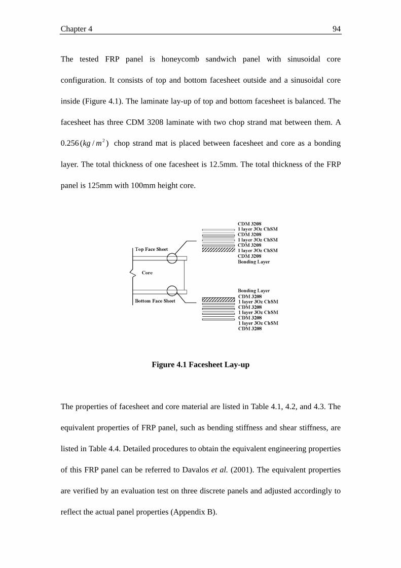
Chapter 4 94
The tested FRP panel is honeycomb sandwich panel with sinusoidal core
configuration. It consists of top and bottom facesheet outside and a sinusoidal core
inside (Figure 4.1). The laminate lay-up of top and bottom facesheet is balanced. The
facesheet has three CDM 3208 laminate with two chop strand mat between them. A
0.256 )/( 2mkg chop strand mat is placed between facesheet and core as a bonding
layer. The total thickness of one facesheet is 12.5mm. The total thickness of the FRP
panel is 125mm with 100mm height core.
Figure 4.1 Facesheet Lay-up
The properties of facesheet and core material are listed in Table 4.1, 4.2, and 4.3. The
equivalent properties of FRP panel, such as bending stiffness and shear stiffness, are
listed in Table 4.4. Detailed procedures to obtain the equivalent engineering properties
of this FRP panel can be referred to Davalos et al. (2001). The equivalent properties
are verified by an evaluation test on three discrete panels and adjusted accordingly to
reflect the actual panel properties (Appendix B).

Chapter 4 95
Table 4.1 Material Properties of Facesheet
Nominal Weight )/( 2mkgThickness
( mm ) fV
o0 0.531 0.49 0.424
o90 0.601 0.55 0.425 CDM 3208
CSM 0.256 0.25 0.396 Bonding Layer ChSM 0.915 1.91 0.188
Table 4.2 Stiffness Properties of Facesheet Lamina
)(1 MPaE )(2 MPaE )(12 MPaG )(23 MPaG 12ν 23ν
CDM 3208 35900 11100 2810 3030 0.305 0.509CDM 3208
CSM 17400 17400 6200 6200 0.406 0.406
Bonding Layer
9820 9820 3510 3510 0.397 0.397
Table 4.3 Stiffness Properties of Facesheet and Core
)(MPaEx )(MPaEy xν )(MPaGxy
Facesheet 13600 14100 0.304 3500 Core 530 1.0 0.431 0.7
Table 4.4 Equivalent Properties of FRP Panel
)(MPaEx )(MPaEy xν )(MPaGxy
In-Plane 2560 2300 0.303 560 Bending 5640 5640 0.303 1400

Chapter 4 96
4.2.2 Steel Stringer
The steel stringers were also modeled by shell elements. The cross bracing is modeled
by two node beam elements. Pin-roller constraint was used to represent the
simply-supported boundary conditions of the test.
4.2.3 Shear Connections
Since the FRP panel connection system displays partial composite action as shown in
test results, the interface movement of panel and stringer needs to be properly
considered in FE model. As illustrated in Chapter 2 and 3, the incomplete interaction
in FRP deck is mainly due to relatively low stiffness of shear connection. In order to
model the shear connection in FE model, the following assumptions are made. The
shear connection is assumed as a connector element with certain length, which is the
distance between the centroid of FRP deck and the centroid of steel top flange. It has
six degree of freedom. Three rotation degrees of freedom are assumed to be restrained.
The distance between FRP panel and steel stringer is assumed to keep unchanged.
This assumption restrains the degree of freedom of vertical translation. The interface
movement is accommodated by allowing degree of freedom of horizontal translation,
which is defined by the stiffness of shear connection (Figure 2.14).
In the FE model, connector elements (CONN32) are used to simulate the actual shear
connection properties. Three rotational components are set to be completely restrained
as well as the vertical translation. Two horizontal translation components are defined

Chapter 4 97
accordingly to the shear connection stiffness and are taken as 1.46kN/mm for a total
interface displacement not to exceed 15 mm.
Figure 4.2 Illustration of Connector Element
Figure 4.3 FE Bridge Model

Chapter 4 98
4.3. FE Analysis Results
As the FRP panel is modeled as a homogeneous solid slab in FE model, global
behaviors of bridge model and T-section modal are straightforward to be obtained,
such as load distribution factor, panel local deflection, effective flange width, and
degree of composite action.
4.3.1 Load Distribution Factor
Similar to bridge model test, the load distribution factors are obtained by using the
expression ∑=
= 3
1ii
iLDFε
ε. The maximum strain values are obtained from shell
element output of steel stringer tension flange at mid-span section. The load
distribution factor is obtained accordingly as the ratio of flange maximum strains.
Compared with experimental data, the FE model appears to be stiffer and the
distribution factor for the center stringer is 0.621. In Chapter 5, an analytical solution
is obtained from a first-term approximate series solution. In the series solution, the
load distribution factor is expressed as function of stringer interaction forces. The
series solution using Eq. (5-33) gives a prediction of about 0.602 and correlates with
the FE and test results fairly well. For the edge loading case, applying the load over
the edge stringer was not possible, and only predicted values are shown in Table 4.5.

Chapter 4 99
Table 4.5 Load Distribution Factor of Bridge Model Connection Spacing 0.6m Diff. (%)
AASHTO LRFD 0.655 1.2 FE model 0.621 -4.0
Series Solution 0.602 -7.0 Phase I Test 0.647
4.3.2 Local Panel Deflection
The panel local deflection of FE model is about L/1039, which is less than test result,
L/726. This result is also within AASHTO LRFD deformation limit for bridge decks,
L/800.
Figure 4.4 Deformed Shape of Panel

Chapter 4 100
-3
-2.5
-2
-1.5
-1
-0.5
0
-1.2 -0.7 -0.2 0.3 0.8
Deformation1
Figure 4.5 Deflection Profile of FRP Panel
Table 4.6 Deflection Profile of Bridge Model 0.6m connection spacing
Deflection Point Deflection (mm) Local Deflection (mm) 1 1.77 2 2.81 1.12 3 1.54 4 0.45 5 0.12
4.3.3 Effective Flange Width
Similarly as shown in the test, the longitudinal normal stress in FRP deck is
non-uniform along its transverse cross section. The normal stress in the deck reaches
the maximum at the mid-line junction of the bridge stringer and deck; and decays
along the deck transverse section away from the junction line. These strain values are
connected linearly to form trapezoidal shape stress blocks. The integral of these stress
blocks, or stress resultant, are the summation of area of each stress block (Figure 4.6).
Effective flange width is then obtained as the ratio of stress resultants to maximum

Chapter 4 101
strain, max1
,max
2/
2/
//)( σσσσ ∑∫=−
==n
iiix
b
bxeff hdxb . The resulted effective flange width is
0.75m, which is about 63% of actual flange width.
maxσ
Figure 4.6 Stress Integration of the Flange
In Chapter 6, the approximate solution for full composite FRP decks is presented for
FRP bridge decks with full composite action. The analytical solution is validated by
FE parametric study. Since the analytical solution only considers full composite action
case, a reduction factor R=0.6 is suggested for the FRP bridge decks with partial
composite action. Thus, applying the factor R to Eq. (6-18), the effective width can be
evaluated as,
)2
cosh(
)cosh(2/
0
b
dyyRb
b
eff ξ
ξ∫= , )(
66
11
AA
aπξ = (4-1)
The corresponding effective flange width is about 0.61m.
Test results and FE show that the actual effective flange width of this T-beam is about
50-65% of actual flange width. More tests on effective flange width and degree of
composite action are suggested. By further test results, the relation between degree of

Chapter 4 102
composite action and effective flange width could be obtained.
4.4. Summary
Overall, the test results correlated well with FE analysis. The predictions of load
distribution factor, effective flange width, and panel local deflection are all within
acceptable range. The simplified FE model adopting equivalent panel properties is
proved to able to define the global behavior of FRP deck bridges.

Chapter 4 103
APPENDIX B: FRP Panel Properties Evaluation
The equivalent properties method (Davalos et al., 2001) is a perfect tool to study the
FRP panel global behavior without involving detailed panel configuration. It avoids
the troublesome to model the actual FRP sandwich configurations in FE model and
remains reasonable accuracy. However, due to the manufacture imperfection and
configuration difference, the actual properties may differ for each FRP panels, which
may further influence the accuracy of FE modeling. Therefore, three FRP panels
(1.8m*2.7m*0.13m) that will be used for the bridge models and T-section model are
evaluated mainly under bending test to obtain the actual properties.
B.1 Test Setup
The FRP panel is simply supported at long span direction, which is 2.7m and is also
the longitudinal core direction, where the sinusoidal core is extended along the span
direction of the panel. The panel width is 1.8m. The panels are loaded by a 245kN
actuator via a 0.6m*0.25m steel plate to the FRP panel (Figure B.1).
Figure B.1 Panel Test Setup

Chapter 4 104
The panels are loaded to 45kN with force control at a loading rate of 9kN/min at 5
different locations, which are numbered from #1 to #5 (Figure B.2). Losition 3 is at
the center of panel. Location 1 and 5 are symmetrically placed at longitudinal
direction and are both 0.3m away from the center line. Location 2 and 4 are
symmetrically placed at transverse direction and are both 0.45m away from the center
line. 5 LVDTs and 10 uni-directional strain gauges are attached at these locations to
measure the vertical displacement, longitudinal and transverse strain of the panel.
Figure B.2 Loading Positions and Instrumentations
B.2 Test Results
The measured panel deflection is presented as mm/kN to provide uniform comparison
data. Similarly, the longitudinal and transverse strains are reduced to microstrain/kN.
The results are shown in Table B.1 and B.2. Label 1L, 2L, 3L, 4L, and 5L represent
the longitudinal strain at location 1 to 5. Label 1T, 2T, 3T, 4T, and 5T represent the

Chapter 4 105
transverse strain at location 1 to 5. At location 4, the strain gauge at transverse
direction is failed and no strain data is available at that position.
Table B.1 Deflection at Location 1 to 5 Test Deflection (10E-2*mm/kN)
Load case 1
(LVDT1)2
(LVDT2)3
(LVDT3)4
(LVDT4)5
(LVDT5) 1.0 -15.3 -15.4 -15.9 -15.7 -12.6 2.0 -14.2 -24.4 -17.5 -12.8 -15.4 3.0 -16.7 -18.2 -19.8 -18.3 -16.9 4.0 -14.1 -12.4 -17.5 -25.0 -15.3 5.0 -12.2 -15.7 -16.1 -16.1 -16.3
Panel 2 -15.0 -18.8 -20.6 -19.4 -17.4 Panel 3 -17.1 -19.6 -21.5 -20.0 -18.4
Table B.2 Longitudinal and Transverse Strain at Location 1 to 5 Test Longitudinal strain (microsrain/kN)
Load case 1L 2L 3L 4L 5L 1 19.5 13.8 9.6 13.2 8.4 2 15.7 27.1 16.6 12.5 15.2 3 13.2 19.4 24.1 19.9 12.9 4 12.4 13.1 14.8 25.4 11.3 5 8.9 14.6 9.1 12.8 18.9
Transverse strain (microsrain/kN) Load case 1T 2T 3T 4T 5T
1 13.9 2.0 7.0 N/A 2.5 2 2.4 10.4 3.1 N/A 2.1 3 6.2 2.8 14.8 N/A 6.2 4 1.7 3.8 2.5 N/A 1.7 5 1.4 1.2 6.8 N/A 13.5
B.3 Comparison of FE Model of FRP Panel and Test Results
An FE model of test panel is constructed by shell element. The FE model simulates
the testing condition and use equivalent properties method to obtain the panel
properties (Table B.3). FE results are compared with test results to obtain the

Chapter 4 106
discrepancy of equivalent properties of panel with actual panel properties. The FRP
panel is modeled by 4 nodes (S4R) shell element with 2D orthotropic properties in
ABAQUS (2002). Same simply supported boundary condition and load condition as
in test is simulated in FE. The deflection and strains data are obtained correspondingly
at location 1 to 5 (Table B.4, Table B.5).
Table B.3 Equivalent Properties of Panel
)(MPaEx )(MPaEy xν )(MPaGxy
In-Plane 2940 2641 0.303 648 Bending 6488 6488 0.303 1600
Table B.4 Deflection Data from FE Model FEM Deflection (10E-2*mm/kN)
Load case 1 2 3 4 5 1.0 -14.0 -13.6 -13.8 -13.6 -10.2 2.0 -13.6 -23.4 -16.8 -11.9 -13.6 3.0 -13.8 -16.8 -18.2 -16.8 -13.8 4.0 -13.6 -11.9 -16.8 -23.4 -13.6 5.0 -10.2 -13.6 -13.8 -13.6 -14.0
Panel 2 -13.8 -16.8 -18.2 -16.8 -13.8 Panel 3 -13.8 -16.8 -18.2 -16.8 -13.8
In Table B.6 and B.7, the deflection and strain data from tests and FE are compared
with each other. Since the load case #1 and #5 are symmetric positioned, it should
give out the duplicated results on deflection and strain. The actual difference in test
data is due to geometry imperfection of the panel and load position. Therefore, the test
data of load case #1 and #5 are averaged. These averaged results are to be compared
with FE load case #1. Similarly, results from load case #2 and #4 are symmetric

Chapter 4 107
positioned. The test data of load case #1 and #5 are averaged and compared with FE
load case #2. This procedure will eliminate the panel imperfection occurred in the
manufacture and possible geometry difference in loading test, such as load position
and support conditions.
Table B.5 Longitudinal and Transverse Strain Data from FE Model FEM Longitudinal strain (microsrain/kN)
Load case 1L 2L 3L 4L 5L 1 18.3 11.7 12.1 11.7 7.1 2 11.4 24.8 16.1 10.6 11.4 3 12.1 16.3 20.8 16.3 12.1 4 11.4 10.6 16.1 24.8 11.4 5 7.1 11.7 12.1 11.7 18.3
Transverse strain (microsrain/kN) Load case 1T 2T 3T 4T 5T
1 12.7 2.2 5.0 2.2 1.7 2 1.2 10.1 0.9 -0.7 1.2 3 5.0 2.3 13.0 2.3 5.0 4 1.2 -0.7 0.9 10.1 1.2 5 1.7 2.2 5.0 2.2 12.7
Table B.6 Deflection Correlation between Test and FE results LC #1 LC #2 LC #3 Panel 2 Panel 3
Location Test FE Test FE Test FE Test FE Test FE 1 -15.9 -14.0 -14.2 -13.6 -16.7 -13.8 -15.0 -13.8 -11.4 -13.8 2 -15.5 -13.6 -24.7 -23.4 -18.2 -16.8 -18.8 -16.8 -19.6 -16.8 3 -16.0 -13.8 -17.5 -16.8 -19.8 -18.2 -20.6 -18.2 -21.5 -18.2 4 -15.9 -13.6 -12.6 -11.9 -18.3 -16.8 -19.4 -16.8 -20.0 -16.8 5 -12.4 -10.2 -15.4 -13.6 -16.9 -13.8 -17.4 -13.8 -18.4 -13.8
Diff (%) 16.7 6.7 13.9 15.0 13.9

Chapter 4 108
Table B.7 Strain Correlation between Test and FE results LC #1 LC #2 LC #3
Strain Loc. Test FE Test FE Test FE 1L 19.2 18.3 14.0 11.4 13.2 12.1 2L 14.2 11.7 26.3 24.8 19.4 16.3 3L 9.4 12.1 15.7 16.1 24.1 20.8 4L 13.0 11.7 12.8 10.6 19.9 16.3 5L 8.6 7.1 13.2 11.4 12.9 12.1
Diff (%) 7.7 12.6 14.7 1T 13.7 12.7 2.1 1.2 6.2 5.0 2T 1.6 2.2 10.4 10.1 2.8 2.3 3T 6.9 5.0 5.3 0.9 14.8 13.0 4T N/A 2.2 -3.8 -0.7 N/A 2.3 5T 1.9 1.7 1.9 1.2 6.2 5.0
Diff (%) 7.2 207.3 20.7
As can be seen, the difference between test data and FE model are consistent for both
deflection and strain. For deflection, the differences between FE and test range from
6.7% to 16.7%. The average difference is that test data are about 13 % larger than FE.
For strain, the difference between test and FE analysis is about 7% to 20% in most of
case. Except for LC#2, at some locations, the transverse strain gauges give out
irregular large strain values, which are due to strain gauge malfunction. The average
difference is that test data are about 13% larger than FE.
All three panels show the similar trend is that the tested panel is actual 13% more
flexible than the equivalent properties method prediction. Therefore, the equivalent
properties of the FRP decks will be divided by a factor of 1.15 ( 15.1%87%100
= ) in
order to compensate for the differences.

Chapter 5 109
CHAPTER 5
EVALUATION OF LOAD DISTRIBUTION
FACTOR BY SERIES SOLUTION
5.1. Introduction
Live load distribution factors (also referred to as girder distribution factors or wheel load
distribution factors) are commonly used by bridge engineers in order to simplify the
complex, three-dimensional behavior of a bridge system. In slab-on-girder bridge design,
the bridge is usually simplified into a T-section and corresponding live load is obtained
by using load distribution factor. This procedure is called beam line analysis in which 3D
problem is simplified into 1D problem.
These factors have been incorporated in American bridge codes since the publication of
the first edition of the AASHTO Standard Specifications in 1931, including the current
specifications (AASHTO, 1996). In 1994, AASHTO adopted the LRFD Bridge Design
Specifications, which contained new formulations of distribution factors that represented
the first major change to these equations since 1931. The relatively recent adoption of
the LRFD specifications has resulted in enhanced accuracy for bridges with geometries
falls into certain applicable limitations. However, for bridges with span lengths, girder

Chapter 5 110
spacing, and other parameters outside of the applicable ranges, overly conservative
results are often obtained. Therefore, there is need to develop distribution factors that can
provide more accurate estimations of live load responses while maintaining simplicity of
form for applications in practice.
5.2. Objectives and Scope
The motivation for this analytical study is to obtain explicit formulas for load distribution
factors for FRP decks over supporting stringers. In this chapter, an approximate series
solution for stiffened plate is presented. The load distribution factor is obtained as ratio of
interaction forces acting over the steel stringers. Then FE parametric study is conducted
on 66 simply-supported slab-on-steel girder bridges. Several parameters, such as span-
length, girder spacing, number of lanes, number of girders, and load conditions are
considered. The impact of these parameters on load distribution factor is investigated by
this parametric study. The FE parametric study is used to validate the accuracy of the
analytical series solution. Based on the FE parametric study, the series solution is used to
obtain multiple regression functions of load distribution factors in terms of non-
dimensional variables. These functions are suitable for design practice.
5.3. Series Solution for Stiffened Plate
An approximate series solution for two-side stiffened orthotropic plate is proposed by
Salim et al. (1995). The analysis procedure is based on macro flexibility approach. The
stiffened plate consists of two major components, slab and stringers, and the slab is

Chapter 5 111
simply supported at two ends and stiffened along the span. The stringers are equally
aligned.
First, the governing equations for slab and stringer elements are obtained separately, for
both symmetric and anti-symmetric load conditions. The deflection formulations of slab
and stringer are contained unknown interaction force at the stringer lines. Then this
unknown interaction force between slab and stringers are solved by ensuring the
displacement compatibility condition at the stringer lines. Lastly, the load distribution
factor of this stiffened plate system is defined as the ratio of single stringer interaction
force to the summation of total stringer interaction force.
5.3.1. Series Solution for Stiffened Plate under Symmetric Load
A two-side stiffened orthotropic plate is shown in Figure 5.1. The plate is stiffened at two
edges along the span ( 0=y , by = ), as well as equally spaced at middle of plate. It is
simply supported at two ends ( 0=x , ax = ). Assumptions are made to simplify the
formulation
(1) no in-plane force or displacement is considered in the formulation;
(2) no torsional moments or stiffness is considered in the stringers;
(3) stringers are equally spaced and have the same section and material properties;

Chapter 5 112
Figure 5.1 Two-side Stiffened Orthotropic Plate with Equally Spaced Stringers
In Macro flexibility approach (Gangarao et al., 1975), the stiffened plate is divided into
two major components, plate element and stringer element. First, the deflection
formulation of plate stiffened with two exterior stringers (Figure 5.2) is obtained from
plate governing equation. The deflection formulation contains one unknown term,
interaction forces R(x,y) at discrete interior stringer lines. Then the deflection
formulation of interior stringers is obtained from stringer governing equations. It contains
the same unknown term, interaction force R(x,y) at discrete stringer lines (Figure 5.3). By
ensuring the displacement compatibility at these interior stringer lines, the deflection
formulation of stiffened plate is solved.
During analysis procedure, the transverse load P is divided into symmetric and
antisymmetric load cases. The deflection formulation and interaction force for symmetric
and antisymmetric load cases are obtained separately. The deflection formulation and
interaction force under asymmetric load P is then obtained by linear superposition.

Chapter 5 113
Figure 5.2 Two-side Stiffened Orthotropic Plate with Exterior Stringers Only
Figure 5.3 Typical Interior Stringer
(a) Orthotropic plate stiffened by exterior stringers only
For the orthotropic plate stiffened by exterior stringers, the governing equation is
),(2 4
4
22
4
4
4
yxqywD
yxwH
xwD yx =
∂∂
+∂∂
∂+
∂∂ (5-1)
here xD is flexural rigidity of plate in x-direction and yD is flexural rigidity of plate in
y-direction; yx νν , is Poisson ratio of plate; H is torsional rigidity of plate and can be
expressed as xyyx DD νν +

Chapter 5 114
The deflection formulation is assumed as
∑ ∑∞
=
∞
=
++++=,...3,2,1 ,...5,3,1
33
2210 ])()()([sinsin),(
i jij b
yCbyC
byCC
byj
axiWyxw ππ (5-2)
And load function is in the form of
∑ ∑∞
=
∞
=
=,...3,2,1 ,...5,3,1
sinsin),(i j
ij byj
axiqyxq ππ (5-3)
In order to simplify the formulation, only first term is taken for the deflection and load
formulation, which is expressed as
])()()([sinsin),( 33
221011 b
yCbyC
byCC
by
axWyxw ++++=
ππ (5-4)
by
axqyxq ππ sinsin),( 11= (5-5)
Since the plate is stiffened at two edges ( byy == ,0 ) and is simply supported at two
ends ( axx == ,0 ). The boundary conditions are
(1) At byy == ,0 , 0=yM with torsinal rigidity and in-plane Poisson’s ratio neglected;
0][ ,02
2
=∂∂
− = byy ywD (5-6)
(2) At byy == ,0 , the interaction force of exterior girder equals to transverse shear
force in the plate,
])4
([][ 2
3
3
3
,04
4
yxw
DD
ywD
xwB
y
xyxybye ∂∂
∂++
∂∂
=∂∂
= νm (5-7)

Chapter 5 115
Substitute deflection formulation (5-4) into boundary condition (5-6), (5-7). All four
unknown coefficients 4321 ,,, CCCC are able to be obtained with 0321 === CCC and
])
4(1
[ 4
2
0 γ
γν
πy
xyx
e
y DD
BDbC
++= .
Therefore, deflection function can be expressed as
)(sinsin),( 011 Cby
axWyxw +=
ππ (5-8)
Substitute deflection formulation (5-8) and load function (5-5) into governing equation
(5-1). The unknown coefficient 11W is then determined as
sDqbW 114
11 )(π
= (5-9)
Where
yxs DHCDD +++= 204 2)41( γπ
γ (5-10)
For a concentrated force P at location 00 , yyxx == , load coefficient 11q is
by
ax
abPq 00
11 sinsin4 ππ= (5-11)
(b) Interior stringers with unknown interaction force
For an interior girder loaded with line load R(x,y), the governing equation is
( nr ,...2,1,0= , n is number of stringers)
),(),(4
4
rxRx
yxwBR
e =∂
∂ (5-12)

Chapter 5 116
The deflection formulation of interior stringer is in similar form as plate deflection
formulation
)(sinsin),( 011 Cnr
axArxwR +=
ππ (5-13)
The applied line load R(x,y) which is the unknown interaction force on the plate is
assumed as
)(sinsin),( 011 Cnr
axRrxR +=
ππ (5-14)
The coefficient 11A is solved by substituting ),(),,( yxRyxwR into governing equation
(5-12)
41111 )(
πa
BRA
e
= (5-15)
(c) Orthotropic plate stiffened by both interior and exterior stringers
The unknown interaction force at stringer lines R(x,y) is solved by ensuring the
displacement compatibility condition between stringers and plate. The plate deflection
equals to the deflection of corresponding stringers. Therefore, the plate deflection
consists of two parts, the deflection induced by transverse load P and the deflection
induced by stringer reaction force R(x,y). Therefore, the equation of plate deflection with
considering this compatibility condition is
∑∫−
=
−=1
1 0
),,,(),(),(),(n a
wR drxKRrxwrxwα
ξαξαξ (5-16)

Chapter 5 117
First term ),( rxw is the plate deflection due to transverse load ),( yxq .
)(sinsin),( 011 Cnr
axWrxw +=
ππ (5-17)
Second term ∑∫−
=
1
1 0
),,,(),(n a
w drxKRα
ξαξαξ is the plate deflection due to stringer reaction
force R(x,y). ),,,( αξrxK w is kernel function solution. In this case, it is the solution for
an arbitrarily located unit load applied at plate where ξ=x and α=y . The first term
approximation of ),,,( αξrxK w is expressed as
)(sinsin),,,( 011 CnrxKrxK w +=π
απαξ (5-18)
Here s
k
DqbK 114
11 )(π
= , kq11 is obtained by substituting 1=P into equation (5-11).
After performing the integration and applying orthognality conditions to (5-16), the
unknown interaction force R(x,y) is solved. The load coefficient 11R is expressed as
)4
1( 04
1111
πγC
bn
BD
qR
e
s ++= (5-19)
Therefore, the generalized deflection function of any interior girder under symmetric
loading is solved as
)(sinsin)(),( 0411 C
nr
axa
BR
rxWe
R +=ππ
π (5-20)

Chapter 5 118
5.3.2. Series Solution for Stiffened Plate under Anti-symmetric Load
Similar procedure is performed for anti-symmetric load case.
(a) Orthotropic plate stiffened by exterior stringers only
For the orthotropic plate stiffened by exterior stringers, the governing equation is
),(2 4
4
22
4
4
4
yxqywD
yxwH
xwD yx =
∂∂
+∂∂
∂+
∂∂ (5-21)
The first term approximation of deflection formulation and load function are expressed in
similar form as for symmetric load case
)]21(2[sinsin),( 112 byC
by
axWyxw −+=
ππ (5-22)
by
axqyxq ππ 2sinsin),( 12= (5-23)
πγνπγ
γν
4)
4()
8(
4)
4(1
24
2
1
xy
xy
y
e
xy
xy
DD
bDB
DD
C++
++
= (5-24)
asDqbW 124
12 )2
(π
= (5-25)
yxas DHC
DD +++= 214 )2
(2)2
1()2
( γπ
γ (5-26)
by
ax
abPq 00
122
sinsin4 ππ= (5-27)
(b) Interior stringers with unknown interaction force
The deflection formulation and interaction force for stringer r is

Chapter 5 119
)]21(2[sinsin),( 112 nrC
nr
axArxwR −+=
ππ (5-28)
)]21(2[sinsin),( 112 nrC
nr
axRrxR −+=
ππ (5-29)
41212 )(
πa
BRA
e
= (5-30)
(c) Orthotropic plate stiffened by interior and exterior stringers
By ensuring the displacement compatibility condition at stringer line, the only unknown
load coefficient 12R is solved in similar fashion as in symmetric load case
)21(16 14
1212
πγC
bn
BD
qR
e
as ++= (5-31)
Therefore, the generalized deflection function of any interior girder under anti-symmetric
loading is expressed as
)]21(2[sinsin)(),( 1412
nrC
nr
axa
BR
rxWe
R −+=ππ
π (5-32)
5.3.3. Series Solution for Stiffened Plate under Asymmetric Load
Since this series solution is for elastic analysis, the deflection formulation of asymmetric
load is obtained by simply superimposing the deflection formulation of symmetric and
anti-symmetric load case.

Chapter 5 120
5.3.4. Load Distribution Factors by Series Solution
After obtain the deflection and stringer force formulation, the load distribution factor is
expressed as ∑+
=
= 1
1
n
r
r
r
R
RLDF . It is the ratio of interaction force on single stringer to the
sum of total interaction force for all stringers.
More specifically, for symmetric load case, the load distribution factor is
∑∑ ==
+
+==
nn
r
symm
Cna
xR
Cnr
axR
rxR
rxRLDF
0 011
011
00
0
)(sinsin
)(sinsin
),(
),(
α
παπ
ππ
(5-33)
For anti-symmetric load case, the load distribution factor is
∑∑ ==
−+
−+==
nn
r
antisym
nrC
naxR
nrC
nr
axR
rxR
rxRLDF
0 112
112
01
1
)]21(2[sinsin
)]21(2[sinsin
),(
),(
α
παπ
ππ
(5-34)
For asymmetric load case, the load distribution factor is
∑∑∑ ===
−+++
−+++=
+
+=
nn
r
n
r
asym
nrC
nrRC
nrR
nrC
nrRC
nrR
rxRrxR
rxRrxRLDF
0 112011
112011
01
00
10
)]}21(2[sin][sin{
)]21(2[sin][sin
),(),(
),(),(
α
ππ
ππ
(5-35)
5.4. Parametric Study on Load Distribution Factors
5.4.1. FE Model Descriptions
Parametric study on typical simply supported slab-on-girder bridge is conducted by using
finite element analysis in order to validate the series solution. A total of 66 concrete slab-

Chapter 5 121
on-steel girder bridges, designed in accordance with the provisions of AASHTO and
West Virginia state guidelines, were modeled and analyzed in ABAQUS (2002). The
following assumptions in finite element modeling are made in order to simplify the
analysis effort while retaining adequate accuracy:
1. The bridge deck is idealized as a horizontal slab of uniform thickness. The material in
the slab is homogeneous, elastic and isotropic;
2. The slab is supported by various numbers of girders. These girders are equally spaced
and are parallel I-shaped steel girders;
3. The edge of the slab and the girder ends are simply supported at the abutments;
4. Full composite action is assumed between the supporting girders and slab. This
means that there is no interface slip at the girder slab interface;
5. No truck wheel load is closer than 0.61m from the roadway edge.
These bridge models consist of two-lane and three-lane bridges. The bridge widths are
9.3m for two-lane bridges and 13.0m for three-lane bridges. For two-lane bridges, the
number of underlying girders is three, four and five, respectively. For three-lane bridges,
the number of underlying girders is four, five and six. These six cross section
configurations are numbered from CS1 to CS6. The corresponding cross section
configurations are shown in Figure 5.4 and Table 5.1. All the bridges are straight bridges
with no skew angle. The major geometrical variables are span-length and girder-spacing.
The selected girder spacing covers the practical range for slab-on-girder bridges. They
are 2m, 2.6m, and 3.5m for two-lane bridges, 2.3m, 2.74m, and 3.5m for thee-lane
bridges. The selected span lengths also cover practical ranges for simply-supported slab-

Chapter 5 122
on-girder bridges. A total of eleven different span lengths were selected. They are varied
from 15.2m to 91.4m, with a 7.6m increment.
Figure 5.4 Typical Cross Section of Bridge Model
Table 5.1 Parameter for Each Cross Section Parameters Two-lane Bridge Three-lane Bridge
CS1 CS2 CS3 CS4 CS5 CS6 A 9.3m 9.3m 9.3m 13.0m 13.0m 13.0m B 8.53m 8.53m 8.53m 12.2m 12.2m 12.2m S 3.51m 2.60m 1.98m 3.51m 2.74m 2.29m ds 1.15m 0.77m 0.69m 1.23m 1.00m 0.77m ts 0.24m 0.20m 0.20m 0.24m 0.22m 0.20m N 3 4 5 4 5 6
Simplified three-dimensional finite element bridge model is adopted. Linear four-node
quadrilateral shell element (S4R) is used to model the concrete slab and steel girders.
Two-node beam element (B31) is used to model diaphragms and cross bracings.
Multiple-point constraint (MPC) rigid element is used to model the shear connection in
the composite bridges (Figure 5.5). This rigid element constrains both rotation and
displacement degree of freedom. It is able to simulate the full composite action in the
bridges. Pin-roller constraint is used to simulate the simply supported boundary condition.
The concrete slab is assumed to be un-cracked and the stiffness does not change during

Chapter 5 123
the loading. No reinforcing steel is considered in the FE model. Therefore, the analysis
limited to static and linear elastic response.
Figure 5.5 Configuration of Finite Elements
5.4.2. Live Load Position
Point load is used to simulate the AASHTO HS20 truck wheel load. For two-lane bridges,
they are loaded with one or two lane HS20 truck load. For three-lane bridges, they are
loaded with one, two, or three lane HS20 truck load (Figure 5.6). The critical longitudinal
and transverse position of truck load need to be decided in order to determine the truck
load position where the maximum moment on critical girders is induced. First, the
longitudinal position of the truck load is defined by using influence lines. This critical
longitudinal position is where the maximum bending moment occurred in the mid-span
section. For simply supported bridge, the location is where the middle axle right on mid-
span line (Figure 5.7).
Muktiple-point constraint rigid elements (MPC)
Web and Flanges (shell Element, S4R)
Concrete Slab (Shell Element, S4R)
Cross-frame Bracing (beam Element, B31)

Chapter 5 124
Figure 5.6 AASHTO HS20 Truck Load for 1-, 2-, and 3- lane Loaded Case
Figure 5.7 AASHTO HS20 Truck Load Longitudinal Position
The critical transverse location of truck load is then evaluated by a preliminary study.
This purpose is to obtain the relation between transverse load location and distribution
factor in critical girder. By this study, the transverse position of the truck load is found
out at where the maximum distribution factor occurred.
As shown in Figure 5.6, the transverse position of the truck is defined by coordinate x,
with origin at a distance which is 0.61m away from the left roadway edge. Then starting
from origin, the truck load is moved to the right at 0.61m interval. The distribution

Chapter 5 125
factors for each girder are obtained at these transverse truck locations. As an example,
Figure 5.8 shows the relation of load distribution factor and wheel load position for a
three-lane bridge with four girder, 30.5m span length, and one-lane truck load. With the
truck load moving to the right, the distribution factor of the left girders decrease and the
distribution factor of the right girders increase (Figure 5.8). In this case, for exterior
girders, the critical transverse wheel load location is x=0 and for interior girders is x =
2.44m. For bridges with other cross section configurations and load conditions, the
critical transverse load positions can be obtained in similar fashion. As discovered by the
preliminary study, exterior girders always have larger distribution factors than interior
girders. For interior girders, the first interior girder next to exterior girder always has the
largest distribution factor.
-0.1
0.0
0.1
0.2
0.3
0.4
0.5
0.6
0.7
0 1 2 3 4 5 6 7 8 9
Distance x (m) (Left of Truck Wheel)
Gird
er D
istri
butio
n Fa
ctor
G1_exteriorG2_interiorG3_interiorG4_exterior
Figure 5.8 Critical Transverse Position for Three-lane Bridge CS4 with 30.5m Span
length (One Lane Loaded)

Chapter 5 126
5.4.3. Load Distribution Factor and FE Results
As suggested by Eom and Nowak (2001), expression j
ii
ii
w
wLDF
∑=
= 3
1ε
ε is adopted to
obtain the load distribution factor from FE model. If the stringers have same section
modulus, which is the case in this study, this expression can be simplified into
NLDF
ii
i
∑=
= 3
1ε
ε. Here iε is the maximum strain at the bottom of the stringer i, N is the
number of lane loaded. Therefore, in FE analysis, the load distribution factor can be
obtained as the ratio of maximum strain of one stringer over the summation of strain
values for all stringers.
5.4.4. Assessment and Discussion of FE Results and Series Solution
Several variables including girder spacing, span length, number of lanes loaded, and
cross section stiffness, are assessed to evaluate their impact on load distribution factor.
The importance of these parameters on load distribution factor is identified.
5.4.4.1. Girder Spacing
In Figure 5.9 and 5.10, it shows the relation between distribution factors and girder
spacing. Figure 5.9 and 5.10 show the distribution factors of the live load moment versus
girder spacing. From FE results, as the girder spacing increases, the load distribution
factor increases. This is mainly due to the increase of tributary area of the deck slab to
girders, i.e. more live load is carried by each girder. By varying the girder spacing from
2.29 to 3.51 m, the live load distribution factor is increased by an average of 14.2% for

Chapter 5 127
0.0
0.1
0.2
0.3
0.4
0.5
0.6
0.7
0.8
0.9
2.2 2.4 2.6 2.8 3.0 3.2 3.4 3.6
Girder Spacing (m)
Dis
tribu
tion
Fact
or
1 Lane Loaded_30.5m_Span2 Lanes Loaded_30.5m_Span3 Lanes Loaded_30.5m_Span1 Lane Loaded_15.2m_Span2 Lanes Loaded_15.2m_Span3 Lanes Loaded_15.2m_Span
Figure 5.9 Influence of Girder Spacing for interior girder with three lanes bridges
(bridge spans 15.2m and 30.5m)
0.0
0.1
0.2
0.3
0.4
0.5
0.6
0.7
0.8
0.9
1.0
2.2 2.4 2.6 2.8 3.0 3.2 3.4 3.6
Girder Spacing (m)
Dis
tribu
tion
Fact
or
1 Lane Loaded_30.5m_Span2 Lanes Loaded_30.5m_Span3 Lanes Loaded_30.5m_Span1 Lane Loaded_15.2m_Span2 Lanes Loaded_15.2m_Span3 Lanes Loaded_15.2m_Span
Figure 5.10 Influence of Girder Spacing for exterior girder with three lanes bridges
(bridge spans 15.2m and 30.5m)

Chapter 5 128
the interior girder and 39.4% for the exterior girder, for the case of one-lane load. Larger
increases resulted for two- and three-lane loaded cases. For example, for three lanes
loaded average increases of 39.6% for the interior and 50.6% for the exterior girders are
obtained. The girder spacing is one of the most important parameters affecting the load
distribution characteristic.
5.4.4.2. Span Length
As illustrated in Figure 5.11 and 5.12, for interior girder, distribution factors decrease as
the span length increases. For exterior girder, distribution factors increase with the span
length increases, but all are within small range. Similar results and trend were found by
other researchers (Bishara et al., 1993; Tabsh and Tabatabai, 2001). Although some
researchers found that span length has significant influence on distribution factor, this
confliction may be due to the reason that in their study the girder cross section remains
constant while span length increasing (Mabsout et al., 1999), which is not realistic in
design practice. It can be concluded that span length has only small effect on load
distribution factor.
5.4.4.3. Number of Lane Loaded
In Table 5.2 and 5.3, the distribution factors for load conditions, one-lane, two-lane, and
three-lane loaded are listed for three-lane bridges, which consist of cross section
configurations of CS4, CS5, and CS6. As expected, with more traffic lanes loaded, the
distribution factor becomes larger. However, multiplied with multi-presence factor, three-
lane loaded cases gives out the maximum load distribution factor for interior girder and

Chapter 5 129
0.4
0.5
0.6
0.7
0.8
0.9
1.0
15 30 45 60 75 90
Span Length (m)
Gird
er D
istri
butio
n Fa
ctor
FE Results
Series Solution
Figure 5.11 Influence of Span Length on Distribution Factor for
Interior Girder with Two-lane Loaded (Cross Section CS4)
0.6
0.7
0.8
0.9
1.0
1.1
1.2
15 30 45 60 75 90
Span Length (m)
Gird
er D
istri
butio
n Fa
ctor
FE Results
Series Solution
Figure 5.12 Influence of Span Length on Distribution Factor for
Exterior Girder with Two-lane Loaded (Cross Section CS4)

Chapter 5 130
two-lane loaded case gives out the maximum load distribution factor for exterior girder
(Figure 5.13, 5.14). This phenomenon also applies to bridges with other cross section
configurations. The number of lanes loaded is determined as the other major parameters
that affects load distribution factors.
Table 5.2 Distribution Factors for Three-lane Bridge (Interior Girder) Number of Lanes Loaded Cross
Section Span(ft) One-lane Two-lane Three-
lane 15.2 0.470 0.709 0.806 38.1 0.448 0.700 0.788 68.6 0.441 0.700 0.782
CS4
91.4 0.433 0.689 0.774 15.2 0.431 0.647 0.676 38.1 0.420 0.639 0.666 68.6 0.418 0.641 0.665
CS5
91.4 0.411 0.632 0.660 15.2 0.394 0.548 0.563 38.1 0.396 0.562 0.563 68.6 0.401 0.565 0.565
CS6
91.4 0.386 0.558 0.561
Table 5.3 Distribution Factors for Three-lane Bridge (Exterior Girder) Number of Lanes Loaded Cross
Section Span(ft) One-lane Two-lane Three-
lane 15.2 0.733 0.900 0.837 38.1 0.725 0.907 0.852 68.6 0.734 0.927 0.872
CS4
91.4 0.718 0.927 0.878 15.2 0.639 0.755 0.686 38.1 0.625 0.763 0.704 68.6 0.631 0.778 0.722
CS5
91.4 0.611 0.777 0.724 15.2 0.538 0.548 0.534 38.1 0.521 0.626 0.571 68.6 0.525 0.637 0.583
CS6
91.4 0.511 0.637 0.586
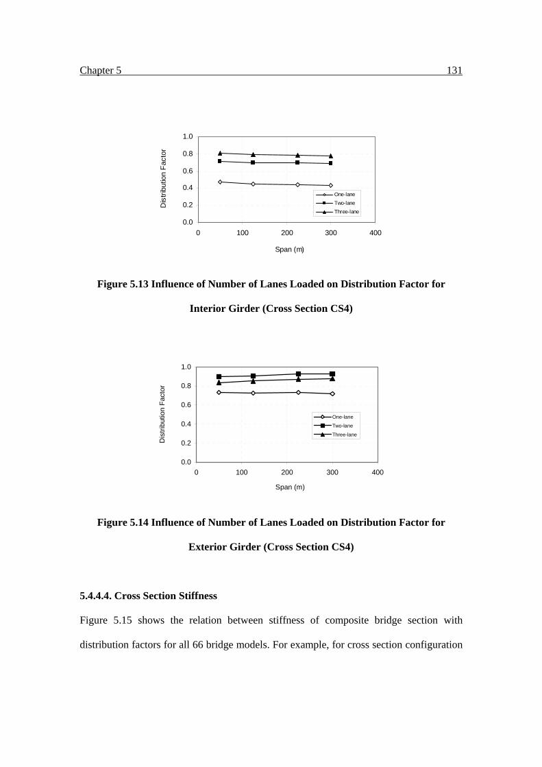
Chapter 5 131
0.0
0.2
0.4
0.6
0.8
1.0
0 100 200 300 400
Span (m)
Dis
tribu
tion
Fact
or
One-laneTwo-laneThree-lane
Figure 5.13 Influence of Number of Lanes Loaded on Distribution Factor for
Interior Girder (Cross Section CS4)
0.0
0.2
0.4
0.6
0.8
1.0
0 100 200 300 400
Span (m)
Dis
tribu
tion
Fact
or
One-lane
Two-lane
Three-lane
Figure 5.14 Influence of Number of Lanes Loaded on Distribution Factor for
Exterior Girder (Cross Section CS4)
5.4.4.4. Cross Section Stiffness
Figure 5.15 shows the relation between stiffness of composite bridge section with
distribution factors for all 66 bridge models. For example, for cross section configuration

Chapter 5 132
CS1, cross section stiffness has only minor effect on distribution factor. With cross
section stiffness increasing, the distribution factor remains almost constant. This also
applies to other cross section configurations. It can be concluded that the cross section
stiffness has only marginal impact on load distribution factor.
0.00
0.10
0.20
0.30
0.40
0.50
0.60
0.70
0.80
0.90
0 100 200 300 400 500 600
Composite Section Moment of Inertia (109mm4)
Gird
er D
istri
butio
n Fa
ctor
1CS
2CS
3CS
4CS
5CS
6CS
Figure 5.15 Influence of Composite Section Moment of Inertia on Distribution
Factors
5.4.5. Comparison of Distribution Factor from Series Solution Formulation and FE
Analysis
Certain assumptions are made in series solution to obtain the load distribution factor. (1)
The HS20 truck is idealized as six asymmetric point loads to represents six wheel loads.
Each point load is further decomposed into symmetric and anti-symmetric load as
required by series solution; (2) The same load position as in FE models are applied in
series solution; (3) No deck overhang and lateral bracing are considered in series solution.
Maple computer program is used to obtain the load distribution factor.
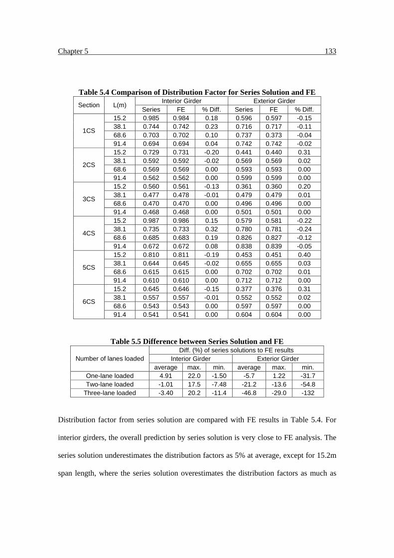
Chapter 5 133
Table 5.4 Comparison of Distribution Factor for Series Solution and FE Interior Girder Exterior Girder Section L(m)
Series FE % Diff. Series FE % Diff. 15.2 0.985 0.984 0.18 0.596 0.597 -0.15 38.1 0.744 0.742 0.23 0.716 0.717 -0.11 68.6 0.703 0.702 0.10 0.737 0.373 -0.04
1CS
91.4 0.694 0.694 0.04 0.742 0.742 -0.02 15.2 0.729 0.731 -0.20 0.441 0.440 0.31 38.1 0.592 0.592 -0.02 0.569 0.569 0.02 68.6 0.569 0.569 0.00 0.593 0.593 0.00
2CS
91.4 0.562 0.562 0.00 0.599 0.599 0.00 15.2 0.560 0.561 -0.13 0.361 0.360 0.20 38.1 0.477 0.478 -0.01 0.479 0.479 0.01 68.6 0.470 0.470 0.00 0.496 0.496 0.00
3CS
91.4 0.468 0.468 0.00 0.501 0.501 0.00 15.2 0.987 0.986 0.15 0.579 0.581 -0.22 38.1 0.735 0.733 0.32 0.780 0.781 -0.24 68.6 0.685 0.683 0.19 0.826 0.827 -0.12
4CS
91.4 0.672 0.672 0.08 0.838 0.839 -0.05 15.2 0.810 0.811 -0.19 0.453 0.451 0.40 38.1 0.644 0.645 -0.02 0.655 0.655 0.03 68.6 0.615 0.615 0.00 0.702 0.702 0.01
5CS
91.4 0.610 0.610 0.00 0.712 0.712 0.00 15.2 0.645 0.646 -0.15 0.377 0.376 0.31 38.1 0.557 0.557 -0.01 0.552 0.552 0.02 68.6 0.543 0.543 0.00 0.597 0.597 0.00
6CS
91.4 0.541 0.541 0.00 0.604 0.604 0.00
Table 5.5 Difference between Series Solution and FE Diff. (%) of series solutions to FE results
Interior Girder Exterior Girder Number of lanes loaded average max. min. average max. min.
One-lane loaded 4.91 22.0 -1.50 -5.7 1.22 -31.7 Two-lane loaded -1.01 17.5 -7.48 -21.2 -13.6 -54.8
Three-lane loaded -3.40 20.2 -11.4 -46.8 -29.0 -132
Distribution factor from series solution are compared with FE results in Table 5.4. For
interior girders, the overall prediction by series solution is very close to FE analysis. The
series solution underestimates the distribution factors as 5% at average, except for 15.2m
span length, where the series solution overestimates the distribution factors as much as

Chapter 5 134
28%. For exterior girders, the differences are larger. For 15.2m span length, the
differences between series solution and FE range from 45% to 67%. For other span
length cases, the differences range from 5% to 28%. Overall, the series solution
underestimates the distribution factor. In Table 5.5, the average, minimum, and maximum
differences are reported for both interior and exterior girders under each load cases.
For the larger differences of exterior girder cases, several factors may contribute to this.
First, the series solution does not take into account the strengthen effect of deck
overhangs brought to the exterior girders. In actual bridge, this strengthen effect will
attract more loads to exterior girder. Secondly, the diaphragm and other secondary
stiffening member have not been taken into account in series solution, which will also
affect the bridge behavior. Overall, the series solutions are reasonably accurate and
efficient for prediction of distribution factors for interior girders.
5.4.6. Application of Series Solution to FRP Deck
The series solution given above was used to obtain load distribution factor for the scaled
bridge model described in Chapter 4. The test specimen consisted of an FRP deck
attached to three steel stringers. Table 5.6 shows close correlation of results. The
favorable results obtained indicate that this solution can be applied to actual bridges in
practice, irrespective of degree of composite action between FRP deck and supporting
stringers.

Chapter 5 135
Table 5.6 Comparison of Distribution Factor for FRP Deck Bridge Model Connection Spacing 0.6m Diff. (%)
AASHTO LRFD 0.655 1.2 FE model 0.621 -4.0
Series Solution 0.602 -7.0 Phase I Test 0.647
5.4.7. Regression Function for Distribution Factor
Based on the parametric study, girder spacing has the most significant impact on load
distribution factor. Moment of inertia of composite section, number of lanes loaded, and
span length are the secondary factors. Therefore, a multiple regression function is
presented. Four non-dimensionalized parameters, the aspect ratio ab , thickness ratio
at ,
flexural rigidity ratio aD
IE bb
⋅, and number of girders N , were selected as independent
variables in multiple regression analysis. An exponential model was defined to conduct
the multiple regression analysis by statistical software. The regression data is based on
the distribution factor from series solution.
As shown from the comparison of series solution and FE, series solution underestimates
the distribution factor in most of load cases, especially for exterior girder with two-lane
and three-lane loaded. Therefore, a modification factors will be applied in the regression
function to gain better results. For exterior girder with one-lane loaded and interior girder
with two- and three-lane loaded, the distribution factors are multiplied by 1.05. For
exterior girder with two-lane loaded and three-lane loaded, the distribution factors are
multiplied by 1.25 and 1.45, respectively.

Chapter 5 136
Therefore the exponential model is
)ln()ln()ln()ln()ln()ln( 43210 NmaD
IEm
atm
abmmDF bb +
⋅+++= (5-36)
the regression function thus can be expressed as
43210 )()()()( mmbbmmm NaD
IEat
abeDF ⋅
⋅⋅⋅⋅= (5-37)
43210 ,,,, mmmmm are constants, and )1(12 2
3
ν−=
tED s , sE , bE are young’s modulus of
slab and beam respectively, ν is slab’s Poisson’s ratio, t is slab thickness, a is span
length, b is slab width, N is girder number. The regression functions of distribution
factors are listed in Table 5.7.
Table 5.7 Regression Function of Distribution Factors Interior Girder
20.012.011.027.0 )()()()(36.1 −××××= NDaEI
at
abDF One-
lane Loaded Exterior
Girder 12.111.069.033.0 )()()()(16.0 −−− ××××= N
DaEI
at
abDF
Interior Girder
16.116.049.095.0 )()()()(89.0 −− ××××= NDaEI
at
abDF Two-
lane Loaded Exterior
Girder 78.114.084.139.1 )()()()(005.0 −−− ××××= N
DaEI
at
abDF
Interior Girder
08.113.005.051.0 )()()()(64.4 −− ××××= NDaEI
at
abDF Three-
lane Loaded Exterior
Girder 88.032.043.055.0 )()()()(15.0 −−−− ××××= N
DaEI
at
abDF

Chapter 5 137
5.5. Summary and Conclusion
A first-term approximate series solution for stiffened plate system is presented. Closed-
form solution is obtained for deck deflection. Distribution factor is then obtained from
this approximate series solution. Then FE parametric study on 66 simply supported slab-
on-girder bridges is conducted. Several major parameters, such as girder spacing, span
length, number of lanes, number of girders, and load conditions are varied in FE model to
study their impact on load distribution factor. The results show that girder spacing is the
predominant variable, while moment of inertia of composite section, number of lanes
loaded, and span length also affect the distribution factor to some extent. By comparing
the distribution factors from FE and series solution, it is found that the series solutions
predict the distribution factor fairly well for interior girder, for which the average
differences are within 5%. For exterior girder, the differences are larger. This is mainly
because the series solution neglects the deck overhang and other secondary strengthening
effect. Using limited experimental data, the series solution provides close values with FE
results for a scaled bridge model, consisting of an FRP deck and steel stringers (see
Chapter 4). The distribution factors from series solution are established as database for a
multiple regression analysis. A set of regression function is presented for bridge design.
As an alternative to FE analysis, the approximate series solutions can be used to conduct
parametric study on large number of bridges. By conducting a preliminary study by FE
analysis, this series solution can be calibrated and then used as a more efficient approach
than FE analysis. Subsequently, regression function can be obtained by the parametric
study and can be used in design practice.

Chapter 6 138
CHAPTER 6
EFFECTIVE FLANGE WIDTH OF FRP
BRIDGE DECKS
6.1. Introduction
In bridge design practice, a deck-and-stringer system acting compositely (i.e., no
interface slippage) is usually simplified as an isolated T-beam section and analyzed by
elementary beam theory, which is usually called beam-line analysis. However, due to in-
plane shear flexibility of the deck or panel section, the longitudinal normal stress in a
bridge deck is non-uniform along its transverse cross section, which is known as shear
lag phenomenon. The normal stress in the deck, along the longitudinal stringer or bridge-
span direction, reaches maximum at the mid-line junction of the bridge stringer and deck;
and the stress decays along the deck transverse section away from the junction line.
Analytical solution for this stress distribution is very cumbersome and not practical for
design. Therefore, effective flange width is defined as an alternative solution to address
shear lag phenomenon in design practice.
Currently, the AASHTO LRFD bridge design specification (2004) includes guidelines for
effective-width of primarily concrete decks to account for shear lag phenomenon. The

Chapter 6 139
effective-width is defined as a reduced width of deck, in relation to center-to-center
spacing of stringers, over which the normal or longitudinal stresses are assumed to be
uniformly distributed as in beam theory for a relatively compact T-beam section.
The studies on FRP bridge decks are mostly based on field- or lab-scale testing results.
Keelor et al. (2004) conducted a field study on a short-span bridge located in
Pennsylvania. This bridge has a pultruded FRP deck over five steel girders equally
spaced at 1.75 m; the span-length is 12.65 m, and the deck thickness is 19.5 cm. The FRP
deck was assumed to achieve full composite-action through grouted stud connections
welded to the stringers. Their results showed that under service load condition, this
design resulted in effective-widths corresponding to about 90% for interior and 75% for
exterior, respectively, of stringer-spacing and half stringer-spacing.
Keller and Gurtler (2005) conducted lab tests on two large scale T-sections to study
composite action and effective-width. Each test model was 7.5 m long with a pultruded
FRP deck section of 1.5 m wide adhesively bonded to the top flange of a steel supporting
beam. The normal strain distribution across the width of the FRP section was recorded at
both upper and lower FRP facesheet components. The results showed that under service
limit state, the normal stress was almost uniform across the panel section. While under
failure limit state, the normal stress decreased towards the panel edges, indicating a more
pronounced effect of shear lag under ultimate load.

Chapter 6 140
6.2. Objectives and Scope
Besides experimental studies as those mentioned above, there is currently no analytical
solution to define effective-deck-width for FRP bridge panels. In this chapter, based on
harmonic analysis developed for FRP thin-walled sections, an approximate effective-
width expression is developed for FRP panels compositely connected to steel supporting
stringers. A finite element analysis of 44 selected FRP deck-and-stringer practical bridges
is conducted to validate the analytical solution for effective-width.
6.3. Shear Lag Model
For full composite-action of FRP-deck over steel-stringer bridges, without considering
the torsional moment in the stringer and the twisting moment in the panel, a section of an
FRP panel stiffened by two steel edge-beams can be isolated as a typical element (Figure
6.1), with edge-stiffeners corresponding to bridge stringer spacing. The panel loaded by
edge shear tractions and axial stress resultants is shown in Figure 6.2.
x
ya
b
Figure 6.1 Typical Panel Element with Two Sides Stiffened

Chapter 6 141
Figure 6.2 Shear flow in Flange Element
Based on equilibrium and boundary conditions at the edges, the panel governing equation
can be solved. Several assumptions are made: (1) the axial force yN and moment yM
are assumed to be zero; (2) the twisting moment in the plate, 0=xyM . By using
equivalent properties, the FRP panel can be represented as an orthotropic plate at
macroscopic scale, with constitute and compliance matrices given as
⎪⎭
⎪⎬
⎫
⎪⎩
⎪⎨
⎧
⎥⎥⎥
⎦
⎤
⎢⎢⎢
⎣
⎡=
⎪⎭
⎪⎬
⎫
⎪⎩
⎪⎨
⎧
x
xy
x
x
xy
x
DA
A
MNN
κγε
11
66
11
000000
(6.1)
⎪⎭
⎪⎬
⎫
⎪⎩
⎪⎨
⎧
⎥⎥⎥⎥⎥⎥⎥
⎦
⎤
⎢⎢⎢⎢⎢⎢⎢
⎣
⎡
=⎪⎭
⎪⎬
⎫
⎪⎩
⎪⎨
⎧
x
xy
x
x
xy
x
MNN
D
A
A
11
66
11
100
010
001
κγε
(6.2)

Chapter 6 142
For an isolated element in the panel (Figure 6.3), the equilibrium equations is
0=∂
∂+
∂∂
yN
xN xyx (6.3)
The compatibility equation is given as
yxxyxyyx
∂∂
∂=
∂
∂+
∂∂ γεε 2
2
2
2
2
(6.4)
Figure 6.3 Isolated Panel Elements
Neglecting the transverse normal strain yε and assuming that xM remains constant along
the y-direction, the panel is not deformable at y-direction and the flexural moment at
panel cross section are constant. Equation (6.3) and (6.4) are substituted into the
compliance matrix (6.2), to obtain the panel governing equation as
0112
2
662
2
11
=∂∂
+∂∂
xN
AyN
Axx (6.5)
This partial differential equation can be reduced to an ordinary differential equation by
using harmonic analysis proposed by Salim and Davalos (2005), which was used to

Chapter 6 143
analyze shear lag in thin-walled open and closed composite beams. The panel in Figure
6.1 is simply supported, or hinged at ax ,0= ; thus, the axial panel force can be defined
as
∑∞
=
=1
)sin()(),(j
jx axjyNyxN π (6.6)
where, )(yN j is an amplitude function. Substituting (6.6) into (6.5) leads to:
jjj N
yN 2
2
2
ξ=∂
∂ , (
66
11
AA
aj
jπξ = ) (6.7)
The general solution for equation (6.7) is given as
)sinh()cosh()( 21 yCyCyN jjjjj ξξ += (6.8)
Where, jC1 and jC2 are determined by compatibility of boundary condition and loading
condition at the stiffened edges of the panel. Therefore, the variation of shear flow can be
expressed as
∑∞
=
+−=∂
∂
121 )cos()]sinh()cosh([
jjjjj
xy
axjyCyC
aj
yN πξξπ (6.9)
From the Mechanics of Laminated Beam model presented by Barbero et al. (1993), the
in-plane shear variation can be defined as
]cos)([)( φByeADxV
yN xy +−=∂
∂ (6.10)
Where, A is the extensional stiffness of the cross section; B is the bending-extension
coupling stiffness, but since an FRP panel is usually designed as symmetric and balanced,
is neglected and set to zero; the term )(ye is the distance between the neutral axis of the
cross section and the middle surface of the flange; )(xV is the resultant shear force acting

Chapter 6 144
on the cross section; D is the cross section bending stiffness; and φ is the orientation of
non-horizontal flange. The in-plane variation of shear y
N xy
∂
∂ can be written in the form of
Fourier series, as
∑∞
=
=∂
∂
1
)cos(j
jxy
axjQ
yN π (6.11)
And the coefficient in Equation (6.11) can be defined as
dxa
xjy
Na
Qa
xyj )cos(2
0
π∫ ∂
∂= (6.12)
Substituting equation (6.10) into (6.12), ( jI depends on loading condition):
jj IaD
yeAQ )(2−= (6.13)
If the origin of the y-axis is located at the center of the cross section, then due to
symmetry, 02 =jC , and equation (6.8) is reduced to
)cosh()( 1 yCyN jjj ξ= (6.14)
By ensuring compatibility of shear flow at the junction of flange and web
( 2/,2/ bby −= ), jC1 can be obtained by equating (6.9) and (6.11). Therefore, the normal
force resultant and normal stress along the panel are
∑∞
=
−=1
)sin(])
2cosh(
)cosh([),(
j j
jjx a
xjby
QjayxN π
ξξ
π (6.15)
AyxN
yx xx
),(),( =σ (6.16)
Based on definition of effective-panel-width, the longitudinal normal stress is assumed to

Chapter 6 145
be uniformly distributed along the panel section, resulting in an equivalent static response
as that caused by the variable stress that in fact exists (Figure 6.4). The effective-width
can be expressed as the integral of normal stress distribution divided by the maximum
stress value at the panel-stiffener intersection:
max
2/
0
max
2/
2/
2
σ
σ
σ
σ ∫∫== −
b
x
b
bx
eff
dxdxb (6.17)
maxσ = maximum stress at junction of deck and stringer. Here, A
yxNyx xx
),(),(max, =σ .
Substituting (6.15) and (6.16) into (6.17), and taking a first-term approximation for
simplicity, the expression for effective-panel-width is given as
)2
cosh(
)cosh(
1
2/
01
b
dyyb
b
eff ξ
ξ∫= (6.18)
Figure 6.4 Effective Flange Width

Chapter 6 146
6.4. Parametric Study on Effective Flange Width
6.4.1. FE Model Descriptions
A total of 44 simple-span FRP-deck and steel-stringer bridges were selected to conduct a
finite element analysis on effective-width. Full composite-action was assumed in all the
bridge models. Bridge cross sections 1CS, 2CS, 3CS, and 4CS were selected and the
bridge deck was an FRP honeycomb panel produced by KSCI. By adopting the
equivalent property method (Davalos et al., 2001), the FRP sandwich panel is idealized
as a structurally orthotropic panel with homogeneous equivalent engineering properties.
This idealized orthotropic panel is then modeled by 4 nodes (S4R) shell element with 2D
orthotropic properties in ABAQUS (2002). The bridge configurations and equivalent
properties for the FRP panel are shown in Table 6.1 and 6.2. Detailed procedure to obtain
the equivalent engineering properties of panel can refer to Davalos et al. (2001).
The number of lanes considered was 2 and 3 with widths of 9.31m for two-lane bridges
and 12.97m for three-lane bridges. The main geometric parameters varied in the study
were span-length and stringer-spacing. The stringer-spacing selected was: 1.98m, 2.59m
and 3.51m for two-lane bridges, and 3.51m for three-lane bridges. A total of 11 span-
lengths were selected from 15.24m to 91.44m, with increments of 7.62m. The bridges
were modeled and analyzed with ABAQUS (2002). The FRP panel and steel I-beam
components were all modeled using shell elements, and beam elements were used to
model the cross frame bracings. Multiple-point constraint (MPC) rigid elements were
used to simulate the interaction between the panel and stringers.

Chapter 6 147
Table 6.1 Parameter for Each Cross Section Parameter CS1 CS2 CS3 CS4
A 9.3m 9.3m 9.3m 13.0m B 8.53m 8.53m 8.53m 12.2m S 3.51m 2.60m 1.98m 3.51m ds 1.15m 0.77m 0.69m 1.23m ts 0.24m 0.20m 0.20m 0.24m N 3 4 5 4
Table 6.2 Equivalent Properties of FRP Panel )(MPaEx )(MPaEy xν )(MPaGxy
In-Plane 2560 2300 0.303 560 Bending 5640 5640 0.303 1400
The following assumptions in finite element modeling are made in order to simplify the
analysis effort while retaining adequate accuracy:
1. The bridge deck is idealized as a horizontal slab of uniform thickness. The material in
the slab is homogeneous, elastic and orthotropic;
2. The slab is supported by variable number of girders. These girders are equally spaced
and are parallel I-shaped steel girders;
3. The edge of the slab and the girder ends are simply supported at the abutments;
4. Full composite action is assumed between the supporting girders and slab. This
means that there is no interface slip at the girder slab interface;
5. No truck wheel load is closer than 0.61m from the roadway edge.
Figure 6.5 Typical Cross Section of Bridge Model

Chapter 6 148
6.4.2. Live Load Position
The AASHTO LRFD service II load combination was applied. From previous research,
the number of lanes loaded had small influence on effective-width, and therefore only
one-lane loaded case was included in the analysis. The live load was positioned
longitudinally at a selected location to induce maximum moment in the bridge models.
For cross section CS1, CS2, and CS3, one- and two-lane loaded cases were selected. For
cross section CS4, one-, two-, and three-lane loaded cases are selected (Figure 6.6).
Figure 6.6 AASHTO HS20 Truck Live Load
6.4. 3. Effective Flange Width Data Reduction from FE Results
max
2/
0
max
2/
2/
2
σ
σ
σ
σ ∫∫== −
b
x
b
bx
eff
dxdxb is defined as a general expression for effective flange width.
To obtain the corresponding effective-width from FE analysis, the integral on the

Chapter 6 149
numerator was obtained by approximation from the FE output. In FE element stress
output, the average normal stress for each shell element ix,σ is uniform along its discrete
length, as shown in Figure 6.7. The height of each rectangle corresponds to the element
longitudinal stress value, and the width is equal to the element mesh size, which is
152mm in this case. Therefore, the integral of the normal stresses, or normal stress
resultant, corresponds to the summation of the discrete values over the panel section. It is
expressed as ∑∑∫==−
==n
iix
n
iiix
b
bx hdx
1,
1,
2/
2/
6 σσσ , where ix,σ is the normal stress of discrete
shell element. Denominator maxσ is the stress value at the panel-stringer center line. The
effective width therefore can be obtained.
maxσ
Figure 6.7 Stress Integration along the Flange Width
6.4.4. Assessment and Discussion of FE Results and Analytical Solution
Several major variables, number of lanes loaded, flange thickness, deck aspect ratio, and
in-plane extensional modulus/shear modulus ratio, are assessed to evaluate their impact
on load distribution factor. The importance of these parameters on load distribution factor
is identified.

Chapter 6 150
6.4.4.1. Number of Lanes Loaded
In order to determine the live load pattern, for 2 lanes bridges CS1, CS2, and CS3, one-
and two-lane loaded cases are selected. For three lanes bridge CS4, one-, two-, and three-
lane loaded cases are selected. For each of these cross section configurations, the
effective width ratio is used as a non-dimensional parameter to facilitate the comparison
instead of using effective width. As can be seen in Table 6.3, the effective flange widths
are very close for bridges with different lanes loaded cases. For CS1 and CS3, which has
symmetrical cross section configuration, the average difference between one-lane loaded
and two-lane loaded cases is within 0.2%. For CS2 and CS4, which has asymmetrical
cross section configuration, the average difference between one-lane loaded and two-lane
loaded cases is within 2%. It is fair to conclude that the number of lanes loaded has only
minor impact on effective flange width. Therefore, all the bridge models in this
parametric study are loaded with only one traffic lane.
Table 6.3 Comparison of Effective Width with Different Number of Lanes Loaded Be/B Be/B Cross Section Span(m) B/L
One-lane Loaded Two-lane Loaded Diff. (%)
15.2 0.230 0.872 0.870 0.290 38.1 0.092 0.953 0.954 -0.098 68.6 0.051 0.974 0.976 -0.174
CS1
91.4 0.038 0.968 0.974 -0.616 15.2 0.170 0.886 0.915 -3.186 38.1 0.068 0.956 0.969 -1.379 68.6 0.038 0.974 0.985 -1.120
CS2
91.4 0.028 0.958 0.973 -1.546 15.2 0.130 0.918 0.918 -0.070 38.1 0.052 0.976 0.975 0.112 68.6 0.029 0.986 0.985 0.042
CS3
91.4 0.022 0.961 0.958 0.316 15.2 0.230 0.812 0.778 4.330 38.1 0.092 0.951 0.935 1.659 68.6 0.051 0.975 0.963 1.202
CS4
91.4 0.038 0.964 0.956 0.875

Chapter 6 151
0.50
0.60
0.70
0.80
0.90
1.00
0.00 0.10 0.20 0.30 0.40 0.50
Flange Width/Span
Effe
ctiv
e Fl
ange
Wid
th/
Act
ual F
lang
e W
idth
2 lane loaded
1 lane loaded
Figure 6.8 Comparison of Number of Lane Loaded for Bridge Section CS1
0.50
0.60
0.70
0.80
0.90
1.00
0.00 0.10 0.20 0.30 0.40 0.50
Flange Width/Span
Effe
ctiv
e Fl
ange
Wid
th/
Act
ual F
lang
e W
idth
2 lane loaded
1 lane loaded
3 lane loaded
Figure 6.9 Comparison of Number of Lane Loaded for Bridge Section CS4
6.4.4.2. Flange Thickness
Based on previous research, flange thickness is generally not a prominent parameter
affecting the effective width. In this FE analysis, cross section CS1 and CS4 have the

Chapter 6 152
same slab thickness of 240mm, while CS2 and CS3 have the same slab thickness of
205mm. However, they do not share the same aspect ratio step. In order to compare these
cross sections directly, by using curve fitting, these models are interpolated and
extrapolated to certain aspect ratio B/L. From comparison, the differences of models with
different slab thickness are small. For example, the difference between CS1 and CS2 is
only 2.1%. For CS3 and CS4, the difference is also small. Therefore, it can be concluded
that within the practical range, the slab thickness is not a major factor on effective width.
6.4.4.3. Aspect Ratio
For span length L and girder spacing B, they are considered as predominant factors that
affect the effective width. They are usually combined into a non-dimensional parameter,
aspect ratio, which is defined as the ratio of girder spacing to span length, LB / . With the
span length increasing, the system shows more beam action. Therefore, effective flange
width increases while LB / decreases (Figure 6.10). The effective width approaches to
full girder spacing when the aspect ratio approach zero. For 1.0/ <LB , the effective
width is larger than 95% of the actual width and effective width ratio 95.0/ >BBe , for
which the effective width is essentially full girder spacing.
6.4.4.4. In-plane Extensional Modulus/Shear Modulus Ratio
As the FRP panel idealized as a homogenous panel with equivalent properties, the in-
plane extensional modulus/shear modulus ratio is 84.3/ =GE for this FRP panel. While
for isotropic material like reinforced concrete, it is usually rated as 4.2)1(2/ =+= νGE .
In other words, the FRP panel is more deformable than concrete slab when it is under in-

Chapter 6 153
plane shear. Therefore, shear lag phenomenon is expected to be more pronouncing in
FRP panel, which will lead to smaller effective flange width.
Table 6.4 Aspect Ratio versus Effective Width CS1 CS2 CS3 CS4
Span(m) B/L Be/B B/L Be/B B/L Be/B B/L Be/B 7.62 0.46 0.643 0.34 0.695 0.26 0.812 0.46 0.636 15.2 0.23 0.872 0.17 0.886 0.13 0.918 0.23 0.856 22.9 0.15 0.916 0.11 0.931 0.09 0.960 0.15 0.914 30.5 0.12 0.950 0.09 0.948 0.07 0.955 0.12 0.932 38.1 0.09 0.953 0.07 0.956 0.05 0.976 0.09 0.947 45.7 0.08 0.965 0.06 0.949 0.04 0.951 0.08 0.947 53.3 0.07 0.967 0.05 0.967 0.04 0.982 0.07 0.963 61.0 0.06 0.971 0.04 0.959 0.03 0.958 0.06 0.942 68.6 0.05 0.974 0.04 0.974 0.03 0.986 0.05 0.971 76.2 0.05 0.970 0.03 0.958 0.03 0.960 0.05 0.956 83.8 0.04 0.973 0.03 0.975 0.02 0.986 0.04 0.974 91.4 0.04 0.968 0.03 0.958 0.02 0.961 0.04 0.957
Table 6.5 Effective Width of FRP Panel and Concrete Panel Be/B Be/B Cross
Section Span(m) B/L Concrete FRP
Diff. (%)
7.62 0.46 0.643 0.551 16.86 38.1 0.09 0.953 0.912 4.51 68.6 0.05 0.974 0.941 3.56
CS1
91.4 0.04 0.968 0.930 4.09 7.62 0.34 0.695 0.642 8.13 38.1 0.07 0.956 0.925 3.36 68.6 0.04 0.974 0.962 1.22
CS2
91.4 0.03 0.958 0.923 3.80 7.62 0.26 0.812 0.762 6.54 38.1 0.05 0.976 0.966 1.03 68.6 0.03 0.986 0.975 1.08
CS3
91.4 0.02 0.961 0.911 5.53 7.62 0.46 0.636 0.537 18.41 38.1 0.09 0.947 0.892 6.21 68.6 0.05 0.971 0.955 1.74
CS4
91.4 0.04 0.957 0.935 2.36

Chapter 6 154
0.60
0.70
0.80
0.90
1.00
0.00 0.10 0.20 0.30 0.40 0.50
Flange Width/Span
Effe
ctiv
e Fl
ange
Wid
th/
Act
ual F
lang
e W
idth
CS1
CS2
CS3
CS4
Figure 6.10 Aspect Ratio vs. Effective Width
0.50
0.60
0.70
0.80
0.90
1.00
0.00 0.10 0.20 0.30 0.40 0.50
Flange W idth/Span
Effe
ctiv
e Fl
ange
Wid
th/
Act
ual F
lang
e W
idth
Concrete
FRP
Figure 6.11 Effective Width of FRP Panel vs. Concrete Panel for Bridge Section CS1
In order to study the effect of modulus ratio on effective width, FE analysis is conducted
on both FRP panel and concrete panel, with the bridge model configurations remain
unchanged. The effective width for both FRP panel and concrete panel are shown in
Table 6.5 and Figure 6.11. The average difference in effective width for FRP and

Chapter 6 155
concrete panel is 5%. The difference becomes larger when the aspect ratio is high. For
7.62m span length and aspect ratio at 0.46, the difference of effective width for FRP and
concrete deck could be as large as 19%. It can be concluded that other than aspect ratio
LB / , the modulus ratio GE / is another factor that affect the effective width.
6.4.5. Comparison between Shear Lag Model and FE Analysis
Effective flange widths from shear lag model are compared with the FE results in Table
6.6. The results show that shear lag model overestimates the effective flange width by an
average error about 6.4%. Overall, shear lag model and FE show similar trend in
effective width prediction. The effective width expression of shear lag model consists of
two major parameters, aspect ratio Lb / and modulus ratio GE / , which is represented as
6611 / AA in shear lag model. In parametric study, these two parameters are determined to
be predominant parameters to affect the effective width. With the aspect ratio decreases,
the effective width increases. When the aspect ratio is less than 0.1, the effective width is
close to 96% of flange width. The largest error is found in model with 7.62m span length,
which is about 8%-14%. For other span length, the effective width from shear lag model
is close to FE analysis.
6.4.6. Comparison between Shear Lag Model and Empirical Function
Tenchev (1996) conducted FE parametric study on effective width for orthotropic flanges.
Boundary conditions, load conditions, and cross section dimensions are the main
variables in his parametric study. Pin-roller and fixed support conditions are considered.
Concentrate and uniformly distributed load conditions are both applied in the FE
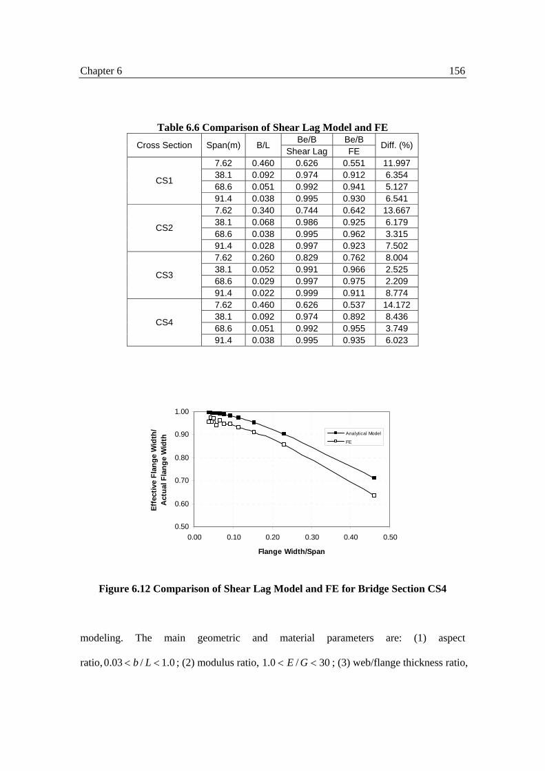
Chapter 6 156
Table 6.6 Comparison of Shear Lag Model and FE Be/B Be/B Cross Section Span(m) B/L
Shear Lag FE Diff. (%)
7.62 0.460 0.626 0.551 11.997 38.1 0.092 0.974 0.912 6.354 68.6 0.051 0.992 0.941 5.127
CS1
91.4 0.038 0.995 0.930 6.541 7.62 0.340 0.744 0.642 13.667 38.1 0.068 0.986 0.925 6.179 68.6 0.038 0.995 0.962 3.315
CS2
91.4 0.028 0.997 0.923 7.502 7.62 0.260 0.829 0.762 8.004 38.1 0.052 0.991 0.966 2.525 68.6 0.029 0.997 0.975 2.209
CS3
91.4 0.022 0.999 0.911 8.774 7.62 0.460 0.626 0.537 14.172 38.1 0.092 0.974 0.892 8.436 68.6 0.051 0.992 0.955 3.749
CS4
91.4 0.038 0.995 0.935 6.023
0.50
0.60
0.70
0.80
0.90
1.00
0.00 0.10 0.20 0.30 0.40 0.50
Flange Width/Span
Effe
ctiv
e Fl
ange
Wid
th/
Act
ual F
lang
e W
idth
Analytical Model
FE
Figure 6.12 Comparison of Shear Lag Model and FE for Bridge Section CS4
modeling. The main geometric and material parameters are: (1) aspect
ratio, 0.1/03.0 << Lb ; (2) modulus ratio, 30/0.1 << GE ; (3) web/flange thickness ratio,

Chapter 6 157
0.3/05.0 << wf TT while wT is varied on two steps; H05.0 and H02.0 . Beam depth
bH 5.0= and span length ftL 7.16= are fixed. 640 FE models are analyzed and
effective widths are obtained. Based on these effective width values, empirical functions
are proposed by curve fitting the FE data. The effective width is represented as effective
width ratio bbe . The empirical function is
416.085.0
21
)()(57.0 −−==GE
Lb
CCbbe
empλ (6.19)
XeC 511 += , GE
LbX 4.6−= (6.20)
YeC 9.02 31.01 −+= , 1))(( −=
Lb
GEY (6.21)
b = actual beam flange width;
L = span length;
E = beam flange Young’s modulus in longitudinal direction;
G = beam flange in-plane shear modulus;
In order to verify the shear lag model, a numerical T-beam model is established with two
major parameters GE / and Lb / varying. Three modulus ratios GE / are selected as 1,
10, and 30. Accordingly, aspect ratio Lb / is varied from (1) 0.1 to 1 at 1/ =GE ; (2)
0.08 to 0.88 at 10/ =GE ; and (3) 0.03 to 0.60 at 30/ =GE . The boundary condition of
this numerical model is set as simply supported and the load condition is set as uniform
distributed load.

Chapter 6 158
The results from shear lag model and empirical function are compared in Table 6.7, 6.8,
and 6.9. At 1/ =GE , the shear lag model consistently overestimates the effective width
than empirical function. Overall, the average error is 6.6% between empirical function
and shear lag model. After 5.0/ <Lb , the predicted effective width from shear lag model
is closer with empirical function (Figure 6.13). At 10/ =GE and 30/ =GE , the shear
lag model has better predictions and the average errors are 1.5% and 3.8%, respectively.
This comparison shows that overall the correlation between shear lag model and
empirical function is good, especially for aspect ratio 5.0/ <Lb . The shear lag model
displays its advantage that it can be applied to the bridges with wider range of parameters,
while maintaining adequate accuracy. Therefore, it is suitable for future design and
parametric study for composite slab-on-girder bridges.
0.20
0.30
0.40
0.50
0.60
0.70
0.80
0.90
1.00
0.00 0.20 0.40 0.60 0.80 1.00
Flange Width/Span
Effe
ctiv
e Fl
ange
Wid
th/
Act
ual F
lang
e W
idth
Empirical Function
Analytical Model
Figure 6.13 Comparison between Shear Lag Model and Empirical Function for
E/G=10
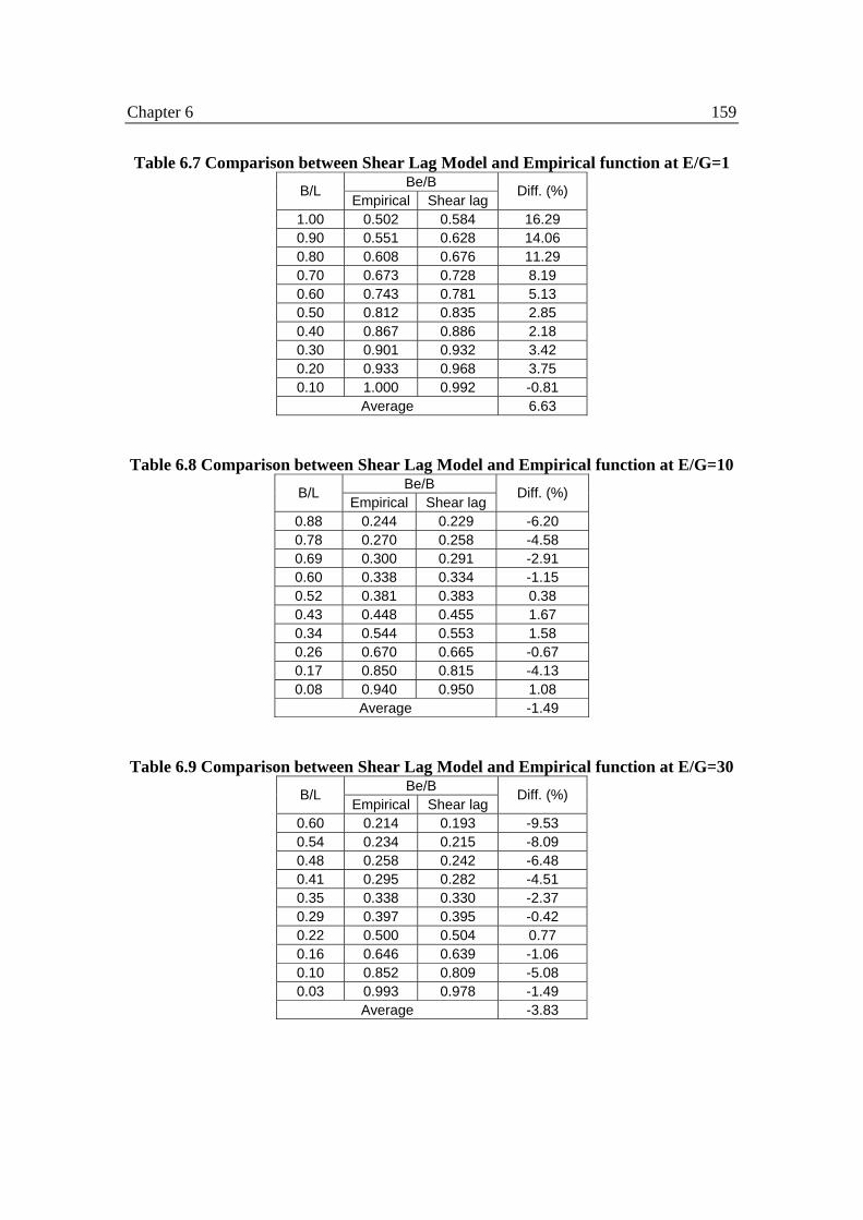
Chapter 6 159
Table 6.7 Comparison between Shear Lag Model and Empirical function at E/G=1 Be/B B/L
Empirical Shear lagDiff. (%)
1.00 0.502 0.584 16.29 0.90 0.551 0.628 14.06 0.80 0.608 0.676 11.29 0.70 0.673 0.728 8.19 0.60 0.743 0.781 5.13 0.50 0.812 0.835 2.85 0.40 0.867 0.886 2.18 0.30 0.901 0.932 3.42 0.20 0.933 0.968 3.75 0.10 1.000 0.992 -0.81
Average 6.63
Table 6.8 Comparison between Shear Lag Model and Empirical function at E/G=10 Be/B B/L
Empirical Shear lagDiff. (%)
0.88 0.244 0.229 -6.20 0.78 0.270 0.258 -4.58 0.69 0.300 0.291 -2.91 0.60 0.338 0.334 -1.15 0.52 0.381 0.383 0.38 0.43 0.448 0.455 1.67 0.34 0.544 0.553 1.58 0.26 0.670 0.665 -0.67 0.17 0.850 0.815 -4.13 0.08 0.940 0.950 1.08
Average -1.49
Table 6.9 Comparison between Shear Lag Model and Empirical function at E/G=30 Be/B B/L
Empirical Shear lagDiff. (%)
0.60 0.214 0.193 -9.53 0.54 0.234 0.215 -8.09 0.48 0.258 0.242 -6.48 0.41 0.295 0.282 -4.51 0.35 0.338 0.330 -2.37 0.29 0.397 0.395 -0.42 0.22 0.500 0.504 0.77 0.16 0.646 0.639 -1.06 0.10 0.852 0.809 -5.08 0.03 0.993 0.978 -1.49
Average -3.83

Chapter 6 160
6.4.7. Application of Shear Lag Model to FRP Deck
The analytical solution was used to obtain effective for the scaled bridge model described
in Chapter 4. The corresponding effective width is about 1.01m. Since the analytical
solution only considers full composite action case, a reduction factor R=0.6 is suggested
for the FRP bridge decks with partial composite action. Thus, applying the factor R to Eq.
(6-18), the effective width can be evaluated as,
)2
cosh(
)cosh(2/
0
b
dyyRb
b
eff ξ
ξ∫= , )(
66
11
AA
aπξ = (6-22)
The corresponding effective flange width is about 0.61m. Also, evaluation by FE analysis
shows the resulted effective flange width of bridge model is 0.75m, which is about 63%
of actual flange width. Test results and FE show that the actual effective flange width of
this T-beam is about 50-65% of actual flange width. More tests on effective flange width
and degree of composite action are suggested. By further test results, the relation between
degree of composite action and effective flange width could be obtained.
6.5. Conclusions
In this chapter, an approximate effective-deck-width expression is developed for FRP
deck and-stringer bridges with full composite-action. By adopting a modification factor R,
the formulation obtained can be modified to accommodate for partial composite action as
shown in section 4.3, Eq. (4.1). A finite element analysis of 44 selected FRP-deck and
steel-stringer bridges is conducted, and the analytical solution for effective-width is
validated by FE results. From the FE parametric study, it can be concluded that effective

Chapter 6 161
width is independent of the number of lanes loaded. Girder spacing and span length are
two major parameters that affect the effective width. These two parameters can be
represented as aspect ratio Lb / . The modulus ratio GE / is another major variable
which will affect the effective width. Comparing with FE, the approximate expression
overestimates the effective width for about 6%. Combined with equivalent orthotropic
properties for FRP cellular and sandwich decks, the proposed analytical expression
provides sufficient accuracy and is relatively simple to be used in design practice. Since
the analytical solution only considers full composite action case, a reduction factor is
suggested for FRP bridge decks with partial composite action.

Chapter 7 162
CHAPTER 7
CONCLUSIONS AND DESIGN
RECOMMENDATIONS
7.1. Conclusions
The major outcomes of the engineered FRP deck-steel stringer bridge system are
summarized in the following sections.
7.1.1. Overview
As the most critical structural component of FRP deck-steel stringer system, a new type
of shear connection is thoroughly studied by push-out test and bridge model test. It is
proved to meet the code requirements for strength and fatigue resistance. Its stiffness,
strength, and fatigue resistance are well defined and used as design basis for FRP bridge
decks. The prototype shear connection also has the ability to transfer shear force at deck-
stringer interface and is expected to achieve a certain degree of composite action.
At the second stage of study, a reduced scale FRP deck bridge model is tested. The bridge
model consists of FRP deck panels, steel supporting stringers, and the proto type shear
connection. The test program consists of three phases. Phase I is a scaled FRP deck

Chapter 7 163
bridge model test with the objectives to study: (1) field deck attachment procedure; (2)
transverse load distribution factors; and (3) local deck deflections and strains. Phase II
test is a bridge model fatigue test with the objectives to evaluate FRP deck-connection
system fatigue behavior. Phase III test is a T-section of 1.2 m wide, which is cut out from
the bridge model, tested to failure. Phase III test focuses on: (1) effective deck-width; (2)
degree of composite action and spacing of connectors; and (3) service-limit and ultimate-
limit states under flexure loads.
The test program is then verified by FE analysis and analytical solutions. A simplified FE
model is constructed which considers partial composite action of the deck. An
approximate series solution on load distribution factor is presented. Then, a harmonic
analysis that was developed for FRP thin-walled sections is formulated to predict the
effective-width of FRP decks.
Based on this study, the engineered FRP deck-steel stringer system is proved to be able to
achieve partial degree of composite action. The structural behaviors, such as degree of
composite action, effective width, load distribution factor, local deflection of panels, are
well defined. Its favorable service limit and ultimate limit performance make the FRP
deck-steel stringer bridge an excellent option for both rehabilitation projects and new
constructions.
7.1.2. Effective Prototype Shear Connection
Through push-out test on both static and fatigue resistance, the load displacement curve

Chapter 7 164
was established as a segmentally linear model. The connection shows good ductility after
yield. The S-N curve was established for this shear connection by fatigue test. The shear
connection was able to sustain cyclic fatigue loading equivalent to 75 years bridge
service life-span. The shear connection was then further tested in a scaled FRP bridge
deck model to evaluate its performance in a bridge system, showing nearly no stiffness
degradation.
During the study, the shear connection shows: (1) the proposed shear connection provides
adequate connectivity for FRP sandwich panels; (2) The shear connection can effectively
transfer shear force between deck and girder while allows certain amount of interface slip.
This property will develop partial composite action in FRP decks; (3) this shear
connection is capable of sustaining cyclic fatigue loading of about 75 years bridge
service-life span under AASHTO live load; (4) the installation process is also
straightforward and easy. The study on prototype shear connection shows that this
connection is structurally efficient and can be used in practice.
7.1.3. Load Distribution Factor
Following shear connection test, a reduced scale FRP bridge model is tested to
investigate the load distribution and local deflection of the FRP panels. The load
distribution factor of interior girders is obtained under concentrate loading condition. The
test results correlate well with FE model analysis. In addition, an analytical solution is
obtained from a first-term approximate series solution. In series solution, the load
distribution factor is expressed as a ratio of stringer interaction force. The series solution

Chapter 7 165
predicts the load distribution factor fairly well with the reference bridge in parametric
study. For interior girders, the prediction is within 5% difference. For exterior girders, the
differences are larger, which is due to neglecting the deck overhang and other secondary
strengthening effect in series solution. The solution is suggested as a simplified method
for load distribution factor.
7.1.4. Panel Local Deflection
In panel local deflection test, the deflection ratio is about L/730. In AASHTO LRFD code,
there is no deflection limit for FRP bridge decks. Many researchers have suggested L/400
as deflection criteria for FRP decks. Therefore, the local deflection for this FRP panel is
considered to be acceptable. One possible solution to reduce the deformation of the FRP
deck is to add horizontal steel bracing between stringers consisting of a supporting grid
under FRP decks. Thus, FRP deck spacing is reduced and the deformation is expected to
be much smaller than the current scheme.
7.1.5. Degree of Composite Action and Effective Flange Width
Degree of composite action and effective flange width are two properties that are
interrelated. For T-beam section, the degree of composite action is about 25% and the
corresponding effective FRP flange width is about 50% of actual width. The distribution
of normal stress proves the existence of shear lag phenomenon in FRP flange. Top
facesheet displays much more pronounced shear lag phenomenon than bottom facesheet,
which is mainly due to low shear transferring capability of the core. Since the core

Chapter 7 166
material does not have much out-of-plane stiffness, the top and bottom facesheet are
mostly act separately under bending action.
An approximate effective flange width expression is developed for FRP bridge decks
with full composite action. The analytical solution is validated by FE parametric study.
Since the analytical solution only considers full composite action case, a reduction factor
is suggested for FRP bridge decks with partial composite action. Test and FE results
show that the actual effective flange width of this T-beam is about 50-65% of actual
flange width. More tests on effective flange width and degree of composite action are
suggested. By further test outcomes, the relation between degree of composite action and
effective flange width would be able to obtain.
7.1.6. Shear Connection Spacing
In reduced scale bridge model test and T-beam test, two different connection spacing,
0.6m and 1.2m, are tested. In terms of structural performance, the difference between
these two connection spacings is only marginal. The difference between these two
connection spacings on service load level, ultimate strength, and degree of composite
action are all within 2%. It is suggested that 1.2m connection spacing may be a good
compromise in cost and performance in FRP bridge decks design.
7.1.7. Service Load and Failure Mode
The failure mode of T-beam is a ductile failure with steel stringer yielding. The ultimate
strength thus mainly depends on the capacity of stringer. At the failure stage, the FRP

Chapter 7 167
panel shows large compression deformation at the loading position where the panel
shows obvious sagging shape. However, there is no visible damage to the FRP panel,
neither at the tongue and groove connection locations. The whole FRP panel remains
intact, as well as the shear connection and steel sleeve. The integrity of whole FRP decks
is provided by both shear connection and tongue and groove connection.
7.2. Summaries
Overall, the test results correlated quite well with FE and analytical solutions. Several
observations and conclusions are made: (1) Using closely-spaced connection spacing (0.6
m instead of 1.2 m) does not significantly improve structural bridge behavior or
performance; thus, a 1.2m connection spacing is adequate and cost-effective in design. (2)
The FRP panel remained visibly undamaged during all tests conducted, including the T-
beam section tested to failure, and also there was no damage observed to the stud-sleeve
connector and the tongue-and-groove connection; thus, the deck-to-stringer and panel-to-
panel connection systems were shown to be structurally efficient concepts for FRP bridge
decks. (3) About 25% degree of composite action was achieved with the prototype shear
connection, which represented an increases of 13% service-load and 7% yield-strength
capacities for the T-beam section compared to non-composite section. (4) For this degree
of composite action, the effective flange width of the T-beam was about 50% of the
actual flange width. (5) The FRP panel local deflections from tests were, respectively,
1.65 mm and 1.75 mm for 0.6 m and 1.2 m connection spacing; the deflection ratio is
about L/730. In AASHTO LRFD code, there is no deflection limit for FRP bridge decks.
Many researchers have suggested L/400 as deflection criteria for FRP decks. Therefore,

Chapter 7 168
the local deflection for this FRP panel is considered to be acceptable. (6) The failure
mode of FRP decks with steel stringers was established in this study as steel stringer
yielding with adequate ductility; the ultimate load mainly depends on the capacity of the
steel stringers. (7) The approximate series solution provided adequate accuracy and
simplicity to be used in design practice. (8) The shear connection and FRP decks showed
more than adequate fatigue resistance to satisfy AASHTO fatigue live load requirement.
7.3. FRP Deck Bridge Design Recommendations and Flow Chart
The basic steps for FRP deck bridge design is outlined here. For FRP deck slab-on-girder
bridges, the general design procedure should follow AASHTO LRFD specification with
corresponding section. The most relevant section is the section for steel bridge structure
design. Certain modifications are highlighted here to address the distinct properties of
FRP deck bridges.
1. For the stud-sleeve type shear connection used, due to its low stiffness, only partial
composite action can be achieved. For FRP bridges with normal span range (~30m),
the shear stiffness of the connection is taken as 1.46 kN/mm. The fatigue stress range
on a single shear connection should be limited to no more than the fatigue stress
threshold, which was established at 53 MPa;
2. For load distribution factors, the approximate series solution can be used as a
simplified analytical method to obtain design factors for interior and exterior girders;
3. For panel local deflection, as for 2.4m girder spacing and 250mm panel thickness, the
local deflection is about L/730. The deformation is considered to be acceptable;

Chapter 7 169
4. The effective flange width is suggested to be taken as about 50% of the actual flange
width of panels (center-to-center spacing of stringers). Consequently, the service load
can be obtained by transform section method;
5. Since the FRP deck is not able to provide full lateral support to the steel compression
flange, the steel stringer should be designed accordingly to ensure its compactness or
prevent flange compression buckling;
7.4. Future Works
Further study on tongue-and-groove connection properties, such as bending strength and
fatigue resistance, is needed to better understand its behavior. Also the in-plane shear
stiffness of the honeycomb sandwich FRP panel needs to be investigated. Because of the
low in-plane shear stiffness of the core, the shear force is distributed unevenly between
the top facesheet and bottom facesheet. The shear transferring mechanism between top
and bottom facesheets is identified as a critical factor for defining effective width as
characterized by shear lag of FRP deck components.

References 170
REFERENCES
AASHTO (1996), AASHTO Standard Specifications for Highway Bridges, 16th Edition, American Association of State Highway and Transportation Officials, Washington D.C. AASHTO (2004), AASHTO LRFD Bridges Design Specifications, 3rd Edition, American Association of State Highway and Transportation Officials, Washington D.C. ABAQUS (2002), User’s Manual, V 6.3, HKS, Inc., RI, USA. Adekola, A.O. (1968), “Effective Widths of Composite Beams of Steel and Concrete”, The Structural Engineer, Vol. 46, No. 9, pp. 285-289. Adekola, A.O. (1974), “The Dependence of Shear Lag on Partial Interaction in Composite Beams”, International Journal of Solids Structures, Vol. 10, pp. 389-400. Ahn, II-Sang, M. Chiewanichakorn, S.S. Chen, and A.J. Aref (2004), “Effective Flange Width Provisions for Composite Steel Bridges”, Engineering Structures, Vol. 26, pp. 1843-1851. Amadio, C., C. Fedrigo, M. Fragiacomo, and L. Macorini (2004), “Experimental Evaluation of Effective Width in Steel-Concrete Composite Beams”, Journal of Constructional Steel Research, Vol. 60, pp. 199-220. Barker, R. M., J. A. Puckett (1997), Design of Highway Bridges, John Wiley & Sons, Inc. Bakht, B., F. Moses (1988), “Lateral Distribution Factors for Highway Bridges”, Journal of Structural Engineering, Vol. 114, No. 8, pp. 1785-1803. Bakht, B., L.G. Jaeger (1990), “Bridge Evaluation for Multipresence of Vehicle”, Journal of Structural Engineering, Vol. 116, No. 3, pp. 603-618. Bakis, C.E., L.C. Bank, V.L. Brown, E. Cosenza, J.F. Davalos, J.J. Lesko, A. Machida, S.H. Rizkalla, and T.C. Triantafillou (2002), “Fiber-reinforced Polymer Composites for Construction – State-of-the-art Review”, Journal of Composites for Construction, Vol. 6, No. 2, pp. 73-87. Bishara, A.G., M. C. Liu, and D. El-Ali Nasser (1993), “Wheel Load Distribution on Simply Supported Skew I-Beam Composite Bridges”, Journal of Structural Engineering, Vol. 119, No. 2, pp. 399-419. Cheung, M.S., M.Y.T. Chan (1978), “Finite Strip Evaluation of Effective Flange Width of Bridge Girders”, Canadian Journal of Civil Engineering, Vol. 5, No. 2, pp. 174-185.

References 171
CSA (1988), Canadian Highway Bridge Design Code (CAN/CSA-S6-88), CSA International. CSA (2000), Canadian Highway Bridge Design Code (CAN/CSA-S6-00), CSA International. Davalos, J.F., H.A. Salim (1993), “Effective Flange Width for Stress-Laminated T-System Timber Bridges”, Journal of Structural Engineering, Vol. 119, No. 3, pp. 938-953. Davalos, J.F., P.Z. Qiao, X.F. Xu, J. Robinson, and K.E. Barth (2001), “Modeling and Characterization of Fiber-reinforced Plastic Honeycomb Sandwich Panels for Highway Bridge Applications”, Composite Structures, Vol. 52, pp. 441-452. Dean, D.L., C. Omid’varan (1969), “Analysis of Ribbed Plates”, Journal of the Structural Division, Proceeding of the American Society of Civil Engineers, Vol. 95, No. ST3, pp. 411-440. Demitz, J. R., Mertz, D. R., and Gillespie, J. W. (2003), “Deflection requirements for bridges constructed with advanced composite materials” Journal of Bridge Engineering, Vol. 8, No. 2, pp. 73-83. Eom, J., A.S. Nowak (2001), “Live Load Distribution for Steel Girder Bridges”, Journal of Bridge Engineering, Vol. 6, No. 6, pp. 489-497. Finch, T.R., J.A. Puckett (1992), Enhancement of Existing Engineering Software, Vol.5-Transverse Load Distribution in Slab-Girder Bridges, Mountain-Plains Consortium Publications 92-9.5, North Dakota State University, ND. Fu, C.C., M. Elhelbawey, M. A. Sahin, and D. R. Schelling (1996), “Lateral Distribution Factor from Bridge Field Testing”, Journal of Structural Engineering, Vol. 122, No. 9, pp. 1106-1109. Gangarao, H.V.S., A.A. Elmeged, and V.K. Chaudhary (1975), “Macroapproach for Ribbed and Grid Plate Systems”, Journal of the Engineering Mechanics Division, Proceeding of the American Society of Civil Engineers, Vol. 101, No. EM1, pp. 25-43. Gangarao, H.V.S., H.J. Farran (1986), “Macro-Element Analysis of Skewed and Triangular Orthotropic Thin Plates with Beam Boundaries”, Computers and Structures, Vol. 22, No. 3, pp. 399-404. Gangarao, H.V.S., V.K. Chaudhary (1988), “Analysis of Skew and Triangular Plates in Bending”, Computers and Structures, Vol. 28, No. 2, pp. 223-235.

References 172
Hays, C.O., L. M. Sessions, and A. J. Berry (1986), “Further Studies on Lateral Load Distribution Using a Finite Element Method”, Transportation Research Record, Vol. 1072, pp. 6-14. Keelor, D.C., Y. Luo, C.J. Earls, and W. Yulismana (2004), “Service Load Effective Compression Flange Width in Fiber Reinforced Polymer Deck Systems Acting Compositely with Steel Stringers”, Journal of Composites for Construction, Vol. 8, No. 4, pp. 289-297. Keller, T., H. Gurtler (2005), “Composite Action and Adhesive Bond between Fiber-Reinforced Polymer Bridge Decks and Main Girders”, Journal of Composites for Construction, Vol. 9, No. 4, pp. 360-368. Keller, T., T. Tirelli (2004), “Fatigue Behavior of Adhesively Connected Pultruded GFRP Profiles”, Composites Structures, Vol. 65, pp. 55-64. Keller, T., H. Gurtler (2005), “Quasi-static and Fatigue Performance of a Cellular FRP Bridge Deck Adhesively Bonded to Steel Girders”, Composites Structures, Vol. 70, pp. 484-496. Kim, S., A. S. Nowak (1997), “Load Distribution and Impact Factors for I-girder Bridges”, Journal of Bridge Engineering, Vol. 2, No. 3, pp. 97-104. Kukreti, A.R., Y. Rajapaksa (1987), “Analysis Procedure for Ribbed and Grid Plate Systems Used for Bridge Decks”, Journal of Structural Engineering, Vol. 116, No. 2, pp. 372-391. Kukreti, A.R., E. Cheraghi (1993), “Analysis Procedure for Stiffened Plate Systems Using An Energy Approach”, Computers and Structures, Vol. 46, No. 4, pp. 649-657. Lopez-Anido, R., H.V.S. Gangarao (1995), “Macroapproach Closed-Form Series Solution for Orthotropic Plates”, Journal of Structural Engineering, Vol. 121, No. 3, pp. 420-432. Mabsout, M.E., K. M. Tarhini, G. R. Frederick, and A. Kesserwan (1999), “Effect of Multilanes on Wheel Load Distribution in Steel Girder Bridges”, Journal of Bridge Engineering, Vol. 4, No. 2, pp. 99-106. Mainstone, R.J., J.B. Menzies (1967), “Shear Connectors in Steel-Concrete Composite Beams for Bridges, Part 1: Static and Fatigue Tests on Push-Out Specimens”, Concrete, Vol. 1, No. 9, pp. 291-302. Mainstone, R.J., J.B. Menzies (1967), “Shear Connectors in Steel-Concrete Composite Beams for Bridges, Part 2: Static and Fatigue Tests on beams”, Concrete, Vol. 1, No. 9, pp. 291-302.

References 173
Moffat, K.R., P.J. Dowling (1975), “Shear Lag in Steel Box Girder Bridges”, The Structural Engineer, Vol. 53, No. 10, pp. 439-448. Moffat, K.R., P.J. Dowling (1978), “British Shear Lag Rules for Composite Girders”, Journal of the Structural Division, Vol. 104, No. st7, pp. 1123-1130. Moon, F.L., D.A. Eckel, and J.W. Gillespie (2002), “Shear Stud Connections for the Development of Composite Action between Steel Girders and Fiber-Reinforced Polymer Decks”, Journal of Structural Engineering, Vol. 128, No. 6, pp. 762-770. Moon, F.L., J.W. Gillespie (2005), “Experimental Validation of a Shear Stud Connection between Steel Girders and a Fiber-Reinforced Polymer Deck in the Transverse Direction”, Journal of Composites for Construction, Vol. 9, No. 3, pp. 284-287. Newmark, N.M., C.P. Siess, and I.M. Viest (1951), “Test and Analysis of Composite Beams with Incomplete Interaction”, Experimental Stress Analysis, Vol. 9, No. 1, pp. 75-92. Nie, J., C.S. Cai (2003), “Steel-Concrete Composite Beams Considering Shear Slip Effects”, Journal of Structural Engineering, Vol. 129, No. 4, pp. 495-505. Oehlers, D.J., M.A. Bradford (1995), Composite Steel and Concrete Structural Members, Elsevier Science Inc. OHBDC (1983), Ontario Highway Bridge Design Code (2nd edition), Ministry of Transportation of Ontario, Canada. OHBDC (1991), Ontario Highway Bridge Design Code (3rd edition), Ministry of Transportation of Ontario, Canada. Park, K.T., S.H. Kim, Y.H. Lee, and Y.K. Hwang (2005), “Degree of Composite Action Verification of Bolted GFRP Bridge Deck-to-Girder Connection System”, Composite Structures, Vol. 72, pp. 393-400. Righman J. (2002), Development of an Innovative connection for FRP Bridge Decks to Steel Girders, Master Thesis, West Virginia University. Righman, J., K.E. Barth, and J.F. Davalos (2004), “Development of an Efficient Connector System for Fiber Reinforced Polymer Bridge Decks to Steel Girders”, Journal of Composites for Construction, Vol. 8, No. 4, pp. 279-288. Salim, H.A., J.F. Davalos, H.V.S. Gangarao, and P.R. Raju (1995), “An Approximate Series Solution for Design of Deck-and-Stringer Bridges”, International Journal for Engineering Analysis and Design, Vol. 2, pp. 15-31.

References 174
Salim, H.A., J.F. Davalos, Pizhong Qiao, and S.A. Kiger (1997), “Analysis and Design of Fiber Reinforced Plastic Composite Deck-and-Stringer Bridges”, Composite Structures, Vol. 38, No. 1-4, pp. 295-307. Shahawy, M., D. Huang (2001), “Analytical and Field investigation of Lateral Load Distribution in Concrete Slab-on-Girder Bridges”, ACI Structural Journal, Vol. 98, No. 4, pp. 590-599. Slutter, R.G., J.W. Fisher (1966), “Fatigue Strength of Shear Connectors”, Highway Research Record, Highway Research Board, Wshington, D.C., No. 147, pp. 65-88. Song, Qi-gen, A.C. Scordelis (1990), “Shear-Lag Analysis of T-, I-, and Box Beams”, Journal of Structural Engineering, Vol. 116, No. 5, pp. 1290-1305. Song, Qi-gen, A.C. Scordelis (1990), “Formulas for Shear-Lag Effect of T-, I-, and Box beams”, Journal of Structural Engineering, Vol. 116, No. 5, pp. 1306-1319. Tabsh, S.W., M. Tabatabai (2001), “Live Load Distribution in Girder Bridges Subject to Oversized Trucks”, Journal of Bridge Engineering, Vol. 6, No. 1, pp. 9-16. Tarhini, K.M., G. R. Frederick (1992), “Wheel Load Distribution in I-Girder Highway Bridges”, Journal of Structural Engineering, Vol. 118, No. 5, pp. 1285-1294. Tenchev, R.T. (1996), “Shear Lag in Orthotropic Beam Flanges and Plates with Stiffeners”, International Journal of Solids Structures, Vol. 33, No. 9, pp. 1317-1334. Zhang, Y., and Cai, C. S. (2007), “Load distribution and dynamic response of multigirder bridges with FRP decks”, Engineering Structures, Vol. 29, No. 8, pp. 1676-1689. Zokaie, T. (2000), “AASHTO-LRFD Live Load Distribution Specifications”, Journal of Bridge Engineering, Vol. 5, No. 2, pp. 131-138.