design evaluation of a duplex circular wet well pumping station
TRANSCRIPT

DESIGN EVALUATION OF A DUPLEX CIRCULAR WET WELL PUMPING STATION UNDER STEADY STATE AND DYNAMIC OPERATING CONDITIONS.
by
James Thomas Mailloux
A Thesis
Submitted to the Faculty
of the
WORCESTER POLYTECHNIC INSTITUTE
In partial fulfillment of the requirements for the
Degree of Master of Science
in
Environmental Engineering

i
ABSTRACT
Duplex Circular Wet Well (DCWW) lifting pump stations are utilized for pumping clear and
solid-bearing liquid. Understanding the effect of design criteria on pump performance is
important to minimize maintenance costs and maximize efficiency. There are currently no known
full-scale laboratory studies that have been performed to investigate the overall design of
DCWWs. The objective of the research was to evaluate the impact of various design criteria, such
as internal geometry and operating conditions on the performance of DCWW pump stations and
provide documentation and recommendations which will be used to augment the current Hydraulic
Institute/American National Standard for Pump Intake Design (ANSI/HI 9.8-1998), (HI)
guidelines. The research was conducted in two phases; Phase 1 consisted of performing a
comparative analysis of the basic flow patterns within the wet well by means of Computational
Fluid Dynamics (CFD), Phase 2 consisted of performing detailed evaluations of various design
aspects on pump performance using a full-scale Physical Model constructed for the research. The
CFD research provided indications regarding potential performance problems that may occur due
to poor flow patterns and potential pump suction swirl, while the physical research provided a
basis for determining the relative advantages of different designs.
The physical research included the evaluation of general flow patterns, free-surface and subsurface
vortices, air entrainment and pump suction swirl. Measurement of the steady state swirl within the
pump showed unacceptable performance in accordance with the HI acceptance criteria. Swirl data
collected under real-world dynamic operating conditions showed that the pump typically did not
experience the adverse conditions indicated at steady state. Normal (symmetrical) pump
orientation resulted in more favorable operation in terms of pump swirl and ingestion of entrained
air than a coplanar (inline) condition. A minimum water elevation was established to minimize
air-entrainment and swirl entering the pumps, reducing possible effects such as cavitation and
vibration of the pump impeller. Air-core subsurface vortices were present under the pumps,
requiring pump-cones to be installed. The collection of real-time dynamic data will allow design
engineers to better understand actual pump performance under normal cycling and clean-out
modes, reducing the operating time under unfavorable conditions and overall maintenance
requirements.
ii
ACKNOWLEDGMENTS
I wish to thank the following people and organizations who helped make this research possible:
First and foremost, I thank the owners of Alden Research Laboratory and their staff for generously
providing financial and technical support, without which this research or Master’s Degree would
not have been possible. Thanks Randy for your patience while I was learning CFD.
Thank you Padu for seeing in me what I doubted in myself.
I thank my thesis advisor Professor Mathisen, for all his advice, teachings and support over the
many years.
My upmost gratitude goes out to Professor Robert Sanks for his financial support, uncanny insight
and guidance on the project. It was a privilege to work with you.
I thank Arnie Sdano of Fairbanks Morse, Pentair Pump Group for the donation of the test pumps
and model tank.
I thank my parents for always believing in me. I hope I’ve made you proud.
I want to thank my children Jesse and Jamie for their support and understanding. Jesse, I couldn’t
have finished the testing without you. We made a good team.
Above all, I thank my wife Karen for her strength, devotion and unwavering support throughout
my many years of school.

iii
NOMENCLATURE
A Area (ft2
Avg Average
)
β Beta Ratio of orifice meter
Cb
C
Pump volute clearance
f
C
Pump bell to floor clearance
w
CFD Computational Fluid Dynamics
Pump volute to wall clearance
Cfs Cubic feet per second
d Diameter of orifice, pump bell or pump suction throat
D Diameter of pump bell or pipe
Ds
Dia Diameter
Sump diameter
DP Differential Pressure
Fr Froude Number
ft Feet
-ft Foot
ft2
ft
Square feet 3
ft·lb Foot pounds
Cubic feet
ft/s Feet per second
g Acceleration due to gravity (32.17 ft/s2
gpm Gallon per minute
)
HI Hydraulic Institute
Hp Horsepower
HWL High water level
IWL Intermediate water level
lbf Pound force
lb/ft2 Pound per square foot

iv
lb/ft3
LWL Low water level
Pound per cubic foot
max Maximum
min Minimum
psi Pound per square inch
Q Flow rate in gpm or cfs
PVC Polyvinyl Chloride
r Radius
Re Reynolds Number
Rev/min Revolutions per minute
Rev/sec Revolutions per second
S Pump bell submergence
s Second
sec Second
SG Specific gravity
T Temperature
Typ Typical
U axial velocity in pump suction throat
V Velocity
Vt
vs. Versus
Tangential velocity
W Weber Number
μ Dynamic viscosity
ν Kinematic viscosity
ρ Density
ω Rotational speed
Γ Circulation
σ Surface tension
‘ As superscript, inch
“ As superscript, feet

v
TABLE OF CONTENTS
ABSTRACT i
ACKNOWELGEMENTS ii
NOMENCLATURE iii
LIST OF FIGURES viii
LIST OF TABLES xiv
1.0 CHAPTER 1 INTRODUCTION ...................................................................................... 1
1.1 BACKGROUND .............................................................................................................. 1
1.2 PROBLEM STATEMENT ............................................................................................... 2
1.3 RESEARCH GOALS ....................................................................................................... 3
2.0 CHAPTER 2 LITERATURE REVIEW .......................................................................... 5
2.1 PUMP STATION DESIGN .............................................................................................. 5
2.1.1 Hydraulic Institute Design Guidelines ........................................................................................................ 5
2.2 HYDRAULIC INFLUENCE ON PUMP PERFORMANCE ......................................... 10
3.0 CHAPTER 3 RESEARCH METHODOLOGY ............................................................ 14
3.1 OVERALL APPROACH ................................................................................................ 14
3.2 CFD MODEL DEVELOPMENT ................................................................................... 14
3.2.1 CFD Baseline Design Geometry ............................................................................................................... 15
3.2.2 CFD Modified Design Geometry ............................................................................................................. 16
3.3 CFD MODELING PROGRAM ...................................................................................... 18
3.3.1 CFD Mesh Generation .............................................................................................................................. 18
3.3.2 CFD Flow-3D Model Setup Parameters ................................................................................................... 20
3.4 PHYSICAL MODEL DEVELOPMENT ....................................................................... 21
3.4.1 Physical Model Description and Setup ..................................................................................................... 21
3.4.2 Instrumentation and Measuring Techniques ............................................................................................. 28
3.4.2.1 Flow ................................................................................................................................................. 28
vi
3.4.2.2 Water Level ...................................................................................................................................... 33
3.4.2.3 Free Surface Vortices ....................................................................................................................... 34
3.4.2.4 Subsurface Vortices ......................................................................................................................... 35
3.4.2.5 Swirl at Impeller Location ............................................................................................................... 36
3.4.2.6 Differential Pressure Cells ............................................................................................................... 39
3.4.2.7 Computer Data Acquisition and Analysis Programs ........................................................................ 40
3.5 PHYSICAL MODEL TEST PROGRAM ...................................................................... 41
3.5.1 HIS Acceptance Criteria ........................................................................................................................... 41
3.5.2 Baseline Geometry and Testing Methodology .......................................................................................... 42
3.5.2.1 Baseline Geometry ........................................................................................................................... 42
3.5.2.2 Testing Methodology ....................................................................................................................... 43
3.5.3 Modified Geometry and Testing Methodology ........................................................................................ 43
3.5.3.1 Modified Geometry .......................................................................................................................... 43
3.5.3.2 Testing Methodology ....................................................................................................................... 46
4.0 CHAPTER 4 RESULTS .................................................................................................. 47
4.1 CFD MODEL RESULTS ............................................................................................... 47
4.1.1 Baseline Geometry .................................................................................................................................... 47
4.1.1.1 Normal Orientation .......................................................................................................................... 47
4.1.1.2 Coplanar Orientation ........................................................................................................................ 52
4.1.1.3 Baseline Summary ........................................................................................................................... 56
4.1.2 Modified Geometry .................................................................................................................................. 57
4.1.2.1 Normal Orientation .......................................................................................................................... 57
4.1.2.2 Coplanar Orientation ........................................................................................................................ 61
4.1.2.3 Modified Design Summary .............................................................................................................. 64
4.2 PHYSICAL MODEL RESULTS ................................................................................... 65
4.2.1 Steady State Testing ................................................................................................................................. 66

vii
4.2.1.1 Baseline Geometry ........................................................................................................................... 67
4.2.1.1.1 Normal Orientation ..................................................................................................................... 67
4.2.1.1.2 Coplanar Orientation .................................................................................................................. 74
4.2.1.2 Modified Geometries ....................................................................................................................... 76
4.2.1.2.1 Installation of Pump Cones ........................................................................................................ 76
4.2.1.2.2 Addition of 45-Degree Fillet ...................................................................................................... 83
4.2.2 Dynamic Testing ....................................................................................................................................... 98
4.2.2.1 Baseline testing ................................................................................................................................ 98
4.2.2.1.1 Normal Orientation ..................................................................................................................... 98
4.2.2.1.2 Coplanar Orientation ................................................................................................................105
4.2.2.2 Addition of 45-Degree Fillet ..........................................................................................................109
4.2.2.2.1 Normal Orientation ...................................................................................................................109
4.2.2.2.2 Coplanar Orientation ................................................................................................................119
4.2.2.2.3 Testing Summary .....................................................................................................................121
4.2.2.3 Cleanout Tests ................................................................................................................................122
5.0 CHAPTER 5 CONCLUSIONS AND RECOMMENDATIONS FOR FUTURE RESEARCH .............................................................................................................................. 124
5.1 CFD CONCLUSIONS .................................................................................................. 124
5.2 PHYSICAL MODEL CONCLUSIONS ....................................................................... 125
5.3 RECOMMENDATIONS FOR FUTURE RESEARCH ............................................... 126
REFERENCES...………………………………………………………………………………137
APPENDIX A CFD MODEL PARAMETERS
APPENDIX B MODEL DETAIL DRAWINGS
APPENDIX C INSTRUMENTATION CALIBRATIONS
viii
List of Figures
Figure 1-1: General layout of a Duplex Circular Wet Well with submersible pumps and sloped sidewalls (HIS 1998) .......................................................................................................2
Figure 2-1: Wet Well Design Guidelines for Clear Liquid Application (HIS 1998) ..........................6
Figure 2-2: Recommended pump bell diameter (HIS 1998) ..............................................................7
Figure 2-3: Recommended pump submergence (HIS 1998) ..............................................................8
Figure 3-1: 3-D solid model utilized for the CFD model study ........................................................15
Figure 3-2: Baseline geometry of the CFD model for the Normal and Coplanar inlet orientations .16
Figure 3-3: Modified design with Normal orientation ......................................................................17
Figure 3-4: Modified design with Coplanar orientation ...................................................................17
Figure 3-5: Plan view showing active mesh blocks with Normal orientation ..................................19
Figure 3-6: Elevation view showing active mesh blocks for Normal orientation and low water condition ........................................................................................................................20
Figure 3-7: Physical model test tank layout ......................................................................................22
Figure 3-8: Plan view of modeled tank assembly .............................................................................24
Figure 3-9: Elevation view of the modeled pump assembly .............................................................25
Figure 3-10: Photograph of the installed pumps and swirl meters ...................................................25
Figure 3-11: Photograph of pumps installed in the normal orientation ............................................26
Figure 3-12: Photograph of pumps installed in the coplanar orientation ..........................................26
Figure 3-13: Model setup and flow loop ...........................................................................................28
Figure 3-14: Guideline for fabrication of an orifice plate meter (ASME 2004) ...............................29
Figure 3-15: 2”, 4” and 6” influent flow meters ...............................................................................31
Figure 3-16: Calibration data of the 2-inch influent meter ...............................................................32
Figure 3-17: Data printout of Alden’s meter selection program .......................................................33
Figure 3-18: Photograph of the Four DP cells and low-level point-gage reference set up ...............34
Figure 3-19: Free-surface vortex classification (Alden) ...................................................................35

ix
Figure 3-20: Subsurface Vortex Classification (Alden) ...................................................................36
Figure 3-21: Modeled swirl meter detail drawing ............................................................................37
Figure 3-22: Relationship of axial to tangential velocity for swirl calculation (Alden) ...................38
Figure 3-23: Influent flow DP cell calibration ..................................................................................40
Figure 3-24: Layout of fillet support ribs and floor cleat .................................................................44
Figure 3-25: Photograph of typical pump cone ................................................................................45
Figure 3-26: Modified wet well geometry in the normal orientation ...............................................45
Figure 3-27: Modified wet well geometry in the coplanar orientation .............................................46
Figure 4-1: Near-surface flow patterns and velocity magnitudes (ft/s) At Elevation 1.25 ft ...........48
Figure 4-2 Wet well centerline flow patterns and velocity magnitudes (ft/s) ...................................49
Figure 4-3: Floor flow patterns and velocity magnitudes (ft/s) At Elevation 0.01 ft ......................50
Figure 4-4: Flow patterns and velocity magnitudes (ft/s), 0.75 ft upstream of pumps .....................51
Figure 4-5: Flow patterns and velocity magnitudes (ft/s) along pump centerlines ..........................51
Figure 4-6: Flow patterns and velocity magnitudes (ft/s), 0.75 ft downstream of pumps ................52
Figure 4-7: Near-surface flow patterns and velocity magnitudes (ft/s) ............................................53
Figure 4-8: Wet well centerline flow patterns and velocity magnitudes (ft/s) .................................54
Figure 4-9: Floor flow patterns and velocity magnitudes (ft/s) ........................................................54
Figure 4-10: Flow patterns and velocity magnitudes (ft/s), 0.75 ft near side of pumps ...................55
Figure 4-11: Flow patterns and velocity magnitudes (ft/s), 0.75 ft far side of pumps ......................55
Figure 4-12 Flow patterns and velocity magnitudes (ft/s) between pumps (looking upstream) ......56
Figure 4-13: Near-surface flow patterns and velocity magnitudes (ft/s At Elevation 1.25 ft ...........58
Figure 4-14: Wet well centerline flow patterns and velocity magnitudes (ft/s) ...............................59
Figure 4-15: Floor flow patterns and velocity magnitudes (ft/s) ......................................................59
Figure 4-16: Flow patterns and velocity magnitudes (ft/s), 0.75 ft upstream of pumps ...................60
Figure 4-17: Flow patterns and velocity magnitudes (ft/s) along the pump centerlines ...................60
Figure 4-18: Flow patterns and velocity magnitudes (ft/s), 0.75 ft downstream of pumps ..............61

x
Figure 4-19: Near-surface flow patterns and velocity magnitudes ...................................................62
Figure 4-20: Wet well centerline flow patterns and velocity magnitudes (ft/s) ...............................62
Figure 4-21 Floor flow patterns and velocity magnitudes (ft/s) .......................................................63
Figure 4-22: Flow patterns and velocity magnitudes (ft/s), 0.75 ft near side of pumps ...................63
Figure 4-23: Floor flow patterns and velocity magnitudes (ft/s), 0.75 ft far side of pumps .............64
Figure 4-24: Flow patterns and velocity magnitudes (ft/s) between pumps (looking upstream) ....64
Figure 4-25: Type 3 Free-surface vortex at pump #2 .......................................................................68
Figure 4-26: Type 6 Free-surface vortex at pump #2 (note the subsurface air-core) .......................69
Figure 4-27 : Type 3 Subsurface vortices under pumps 1 & ............................................................70
Figure 4-28: Pump 1 swirl angles, normal orientation, baseline geometry ......................................72
Figure 4-29: Pump 2 swirl angles, normal orientation, baseline geometry ......................................74
Figure 4-30: Pump 1 swirl angles, normal orientation, baseline geometry with and without pump cones ..............................................................................................................................78
Figure 4-31: Pump 2 swirl angles, normal orientation, baseline geometry with and without pump cones ..............................................................................................................................79
Figure 4-32: Pump 1 swirl angles, coplanar orientation, baseline with cones ..................................81
Figure 4-33: Pump 2 swirl angles, coplanar orientation, baseline with cones ..................................82
Figure 4-34: Pump 1 swirl angles, normal orientation, modified geometry .....................................85
Figure 4-35: Pump 2 swirl angles, normal orientation, modified geometry .....................................87
Figure 4-36: Pump 1 swirl angles, coplanar orientation, modified geometry ..................................90
Figure 4-37: Pump 2 swirl angles, coplanar orientation, modified geometry ..................................92
Figure 4-38: Influent flow diverter modification ..............................................................................93
Figure 4-39: Pump 1 swirl angles, normal orientation, modified geometry with and without a flow diverter ...........................................................................................................................95
Figure 4-40: Pump 2 swirl angles, normal orientation, modified geometry with and without a flow diverter ...........................................................................................................................96
Figure 4-41: Compilation graph of Pump 1 dynamic swirl, normal orientation Baseline geometry 100
xi
Figure 4-42: Dynamic Pump 1 swirl angles, 0-gpm, normal orientation, baseline ........................100
Figure 4-43: Dynamic Pump 1 swirl angles, 25-gpm, normal orientation, baseline ......................101
Figure 4-44: Dynamic Pump 1 swirl angles, 125-gpm, normal orientation, baseline ....................101
Figure 4-45: Compilation graph of Pump 2 dynamic swirl, normal orientation Baseline geometry 103
Figure 4-46: Dynamic Pump 2 swirl angles, 0-gpm, normal orientation, baseline ........................103
Figure 4-47: Pump 2 swirl angles, 25-gpm, normal orientation, baseline ......................................104
Figure 4-48: Dynamic Pump 2 swirl angles, 125-gpm, normal orientation, baseline ....................104
Figure 4-49: Compilation graph of Pump 1 dynamic swirl, coplanar orientation Baseline geometry 106
Figure 4-50: Dynamic Pump 1 swirl angles, 0-gpm, coplanar orientation, baselin ........................106
Figure 4-51: Dynamic Pump 1 swirl angles, 25-gpm, coplanar orientation, baseline ....................107
Figure 4-52: Dynamic Pump 1 swirl angles, 125-gpm, coplanar orientation, baseline ..................107
Figure 4-53: Compilation graph of Pump 2 dynamic swirl, coplanar orientation Baseline geometry 108
Figure 4-54: Compilation graph of Pump 1 dynamic swirl, normal orientation Modified geometry 110
Figure 4-55: Dynamic Pump 1 swirl angles, 0-gpm, normal orientation Modified geometry: ......111
Figure 4-56: Dynamic Pump 1 swirl angles, 25-gpm, normal orientation Modified geometry .....111
Figure 4-57: Dynamic Pump 1 swirl angles, 25-gpm, normal orientation Modified geometry ....112
Figure 4-58: Dynamic Pump 1 swirl angles, 125-gpm, normal orientation Modified geometry ..112
Figure 4-59: Dynamic Pump 1 swirl angles, 25-gpm, normal orientation Modified geometry with flow diverter ................................................................................................................113
Figure 4-60: Dynamic Pump 1 swirl angles, 125-gpm, normal orientation Modified geometry with flow diverter ................................................................................................................114
Figure 4-61: Compilation graph of Pump 2 dynamic swirl, normal orientation Modified geometry 115
Figure 4-62: Dynamic Pump 2 swirl angles, 0-gpm, normal orientation Modified geometry .......116
Figure 4-63: Dynamic Pump 2 swirl angles, 25-gpm, normal orientation Modified geometry .....116
Figure 4-64: Dynamic Pump 2 swirl angles, 25-gpm, normal orientation Modified geometry .....117
Figure 4-65: Dynamic Pump 1 swirl angles, 125-gpm, normal orientation Modified geometry ...117

xii
Figure 4-66: Dynamic Pump 1 swirl angles, 25-gpm, normal orientation Modified geometry with flow diverter ................................................................................................................118
Figure 4-67: Dynamic Pump 1 swirl angles, 125-gpm, normal orientation Modified geometry with flow diverter ................................................................................................................119
Figure 4-68: Compilation graph of Pump 1 dynamic swirl, coplanar orientation Modified geometry ......................................................................................................................120
Figure 4-69: Compilation graph of Pump 2 dynamic swirl, coplanar orientation Modified geometry ......................................................................................................................121

xiii
List of Tables
Table 2-1: Maximum Flow Rates for Influent Piping (Sanks 2008) ................................................10
Table 3-1: Modeled and HI Recommended Wet Well Parameters ...................................................27
Table 3-2: Flow Meter Selection ......................................................................................................30
Table 4-1: Steady State Swirl Repeatability Data .............................................................................66
Table 4-2: Initial Recorded Swirl Angles .........................................................................................71
Table 4-3: Recorded Swirl Angles at Pump #1 Normal Orientation, Baseline Geometry ...............72
Table 4-4: Recorded Swirl Angles for Pump #2 Normal Orientation, Baseline Geometry .............73
Table 4-5: Initial Recorded Swirl Angles Coplanar Orientation, Baseline Geometry .....................76
Table 4-6: Recorded Swirl Angles for Pump 1 Addition of Pump Cones, Normal Orientation ......77
Table 4-7: Recorded Swirl Angles for Pump 2 Addition of Pump Cones, Normal Orientation ......79
Table 4-8: Recorded Swirl Angles for Pump 1 Pump Cones, Coplanar Orientation .......................80
Table 4-9: Recorded Swirl Angles for Pump 2 Pump Cones, Coplanar Orientation .......................82
Table 4-10: Recorded Swirl Angles for Pump 1 45-Degree Fillet & Pump Cones, Normal Orientation .....................................................................................................................85
Table 4-11: Recorded Swirl Angles for Pump 2 45-Degree Fillet & Pump Cones, Normal Orientation .....................................................................................................................86
Table 4-12: Recorded Swirl Angles for Pump 1 45-Degree Fillet & Pump Cones, Coplanar Orientation .....................................................................................................................89
Table 4-13: Recorded Swirl Angles for Pump 2 45-Degree Fillet & Pump Cones, Coplanar Orientation .....................................................................................................................91
Table 4-14: Recorded Swirl Angles for Pump 1 45-Degree Fillet, Pump Cones & Flow Diverter Normal Orientation ........................................................................................................94
Table 4-15: Recorded Swirl Angles for Pump 2 45-Degree Fillet, Pump Cones & Flow Diverter Normal Orientation ........................................................................................................96
Table 4-16: Pump 1 Cleanout Results ............................................................................................123
Table 4-17: Pump 2 Cleanout Results ............................................................................................123

1
1.0 CHAPTER 1
INTRODUCTION
1.1 BACKGROUND
Pump stations designed with a circular wet well footprint are frequently used for pumping both
clear and solid bearing liquids. The advantage to a circular design is its relatively small footprint
per corresponding wet well volume, as well as its relative ease of construction. These stations
may range in size from as small as 3 feet in diameter to as great as (+)100 feet in diameter and
may have anywhere from one to (+)10 pumps, with pump flows ranging from hundreds to
thousands of gallons per minute per pump. Smaller wet wells are typically prefabricated and may
be delivered to the site fully assembled, or in the case of a larger unit, assembled on site. The
more commonly used circular pump stations are the Triplex (3 pumps) and Duplex (2 pumps)
configurations.
Duplex Circular Wet Wells (DCWW) fitted with solid-handling pumps, are utilized for the
transference of solid-bearing fluids from system conduits to facilities designed for enhanced
treatments. Typical applications include wastewater, raw water, stormwater, combined
wastewater and industrial wastewater. Fluid is transported to the wet well by means of a closed-
conduit pipe which may be hundreds of feet long. Since the fluid may be solid-bearing, the pumps
must be able to handle both settling and suspended solids, as well as floatables. The station must
be able to self clean for continuous pumping operation, which includes the removal of settled
solids and surface scum. The designated pumps may be vertical-axial, dry-pit centrifugal or fully
submersible centrifugal in design. The pump selection is typically dependent on the
characteristics of the liquid, solids, site geometry and preference of the design engineer.
These pump stations are typically installed in sub-divisions and therefore, are automated in
operation. Pump activation is triggered by high-water and low-water limit switches in the wet
well, with pumping frequency dependent on influent factors such as water use and storm events.
Logic-control panels may be used to alternate the operation cycling of the pumps, thereby
reducing maintenance requirements. Constant-speed pumps are commonly utilized in station
design, as they are more economical to install and operate. Pump capacity is selected so that a

2
single pump exceeds the normal maximum influent rate; thereby assuring that only one pump is
required for normal operation. Additional pumps are brought online as required during peak
events. Since design inflow is less than pump capacity, operation of these stations is typically
dynamic in nature, with the drawdown rate being influent-flow dependent. A general layout of a
DCWW with two submersible pumps is shown in Figure 1-1.
Figure 1-1: General layout of a Duplex Circular Wet Well with submersible pumps and sloped sidewalls (HIS 1998)
1.2 PROBLEM STATEMENT
General guidelines for the design of generic duplex and triplex circular wet wells currently exist
under the Hydraulic Institute/American National Standard for Pump Intake Design (ANSI/HI 9.8-
1998), (HI). However, hydraulic model studies of the wet well are only required by the HI for
larger stations containing pumps with capacities of 5,000 gpm/pump (or higher), or with four or
3
more pumps in the design. This is due to the reasoning that the cost of the smaller station doesn’t
warrant the expense of conducting a model study. However, as there could be thousands of these
stations installed throughout the country, the cost of premature pump failure due to poor
performance could be significant. Further discussion on the HI guidelines for circular pump
stations is presented in Section 2.1.1.
There are no known full-scale laboratory studies that have been performed to investigate the
overall design of smaller DCWWs. Consequently, it is unclear as to the impact of various design
criteria, such as internal geometry and operating conditions, on the performance of the station in
terms of general flow patterns, free-surface and subsurface vortices, air entrainment and pump
suction swirl. Field observations, although insightful, supply the observer with limited
information with regard to these crucial hydraulic performance criteria, as the only thing that is
visible is the water surface. In addition, observations would be required at varying times during
the day, week and year in order to fully assess the operation of the installed design. If operating
conditions are found to be unfavorable, on-site modifications would need to be performed and the
station re-evaluated. Unlike field-testing, where conditions are dynamic and operation sporadic,
laboratory testing allows for in-depth research to be conducted under controlled conditions.
Design modifications can be installed and evaluated under selected operating conditions, allowing
for direct comparative analyses of various designs to be conducted within a relatively short
timeframe.
1.3 RESEARCH GOALS
This thesis describes a laboratory research program initiated to evaluate the impact of design
modifications using the controlled conditions that cannot be obtained in the field. The goal of the
research was to study the impact of various design parameters on hydraulic performance and
floatables removal capability, by means of modeling, and provide documentation and
recommendations which could be used to augment the current HI design guidelines.
The evaluation of various design aspects were conducted under two phases. Phase 1 consisted of
performing a comparative analysis of the basic flow patterns within the wet well by means of
Computational Fluid Dynamics (CFD) for a baseline and modified design, Phase 2 consisted of

4
performing detailed evaluations of various design aspects (flow and geometry) on pump
performance using a Physical Model testing approach. Testing was performed under both steady
state (Qin = Qout) and dynamic operating conditions (Qin < Qout
Discussions on pump station design, including the HI recommended criteria and associated
background theory is covered in Chapter 2. The CFD modeling approach and methodology is
covered in Sections 3.1 and 3.2. The physical model development and research methodology are
covered in Section 3.4 and the test program, including the HI acceptance criteria are covered in
Section 3.5. Results of the CFD simulations and physical testing are presented in Chapter 4.
Conclusions and recommendations for future research are discussed in Chapter 5.
). Basic variables included influent
flow, pump orientation (symmetrical or inline), internal geometry of the wet well (side slope
angle, cones, etc.) and operating water level. Although various pump types are utilized in these
stations, this research focused on submersible centrifugal pumps, as studying all the recommended
wet well designs was beyond the scope of this paper.

5
2.0 CHAPTER 2
LITERATURE REVIEW
2.1 PUMP STATION DESIGN
The Hydraulic Institute Standards (HIS) for Pump Intake Design was developed for use by
manufacturers, design engineers and end users, to assist them in the development and selection of
appropriate design criteria for a given operating condition. The Hydraulic Institute (HI) was
formed under the American National Standards Institute and consisted of approximately twenty
committee members representing manufacturers, researchers and end users. The adopted
standards were reviewed by approximately fifty organizations prior to approval.
It is of the consensus of the HI that unfavorable hydraulic operating conditions can have an
adverse affect on pump performance (see Section 2.2 for further discussion on hydraulic
influences on pump operation).
2.1.1 Hydraulic Institute Design Guidelines
The HI design guidelines for DCWW’s for solid-bearing liquids follow the same baseline criteria
as for clear liquids, with the pumps centered in the wet well as shown in Figure 2-1. Selection of
governing parameters needs to be made based on pump type. In the case of submersible pumps,
Db refers to the volute diameter and in vertical pumps, the bell diameter. However, the term D,
without any suffixes, always refers to the bell diameter, regardless of pump type. Setting the
design criteria based on the pump bell and volute assures that the wet well will be properly sized
regardless of pump selection.
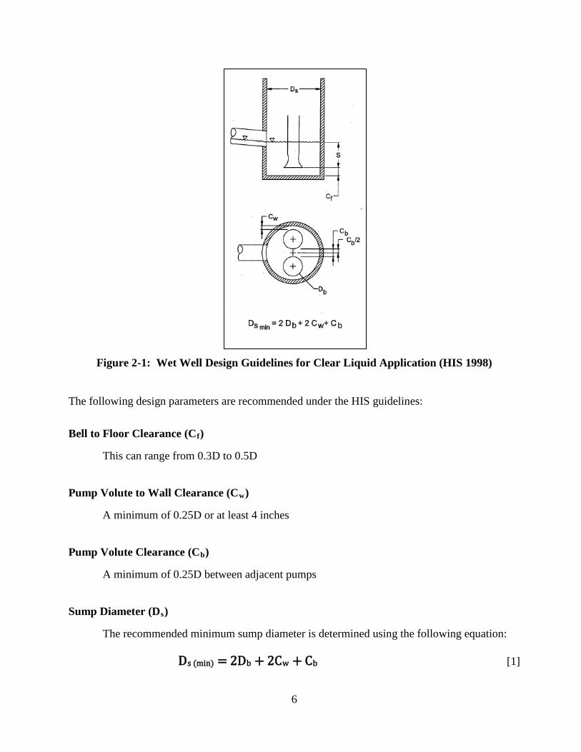
6
Figure 2-1: Wet Well Design Guidelines for Clear Liquid Application (HIS 1998)
The following design parameters are recommended under the HIS guidelines:
Bell to Floor Clearance (Cf
This can range from 0.3D to 0.5D
)
Pump Volute to Wall Clearance (Cw
A minimum of 0.25D or at least 4 inches
)
Pump Volute Clearance (Cb
A minimum of 0.25D between adjacent pumps
)
Sump Diameter (Ds
The recommended minimum sump diameter is determined using the following equation:
)
Ds (min) = 2Db + 2Cw + Cb [1]

7
Pump Bell Diameter (D)
Pump bell shape and size are determined by each manufacturer, resulting in a range of
diameters for the same flow capacity. Each manufacturer may also offer various bell
configurations depending on the pump type and application. Realizing this, the HI created
the graph shown on Figure 2-2, which contains recommendations for bell diameter, as
based on a corresponding bell velocity (in ft/s) for a given flow. Recommended pump bell
velocities range from 2 ft/s to 9 ft/s.
Figure 2-2: Recommended pump bell diameter (HIS 1998)
Pump Bell Submergence (S)
The recommended minimum submergence can be determined using the following
equation:
S = D + 0.574Q/D1.5
[2]
where: S = inches, Q = flow (gpm), and D = bell diameter (inches)
Since the pump bell selection is related to velocity, the HI also created the graph shown on
Figure 2-3, which contains recommendations for submergence as based on a
corresponding bell diameter and velocity for a given flow.

8
It should be noted that the recommended minimum submergence is based on uniform flow
approaching the pump, which circular wet wells may not possess without the installation of
flow-straightening devices. Consequently, the actual required minimum submergence may
differ.
Figure 2-3: Recommended pump submergence (HIS 1998)
Inflow Pipe
Only general recommendations are made for the position and orientation of the inflow
pipe. The pipe shall have no bends, valves or fittings within five pipe-diameters directly
upstream of the wet well. The pipe is not to be positioned higher than shown in Figure 2-
1. However, as this is only a graphical representation, it is unclear as to the precise
location. It stands to reason that the higher the pipe, the greater the amounts of air
impingement, due to the free-discharge impinging on the water surface at lower water
elevations. There is no recommendation for the slope of the pipe. It is recommended that
the placement of the pipe is radial to the tank and perpendicular (normal) to the centerline
of the pumps to reduce rotational flow patterns. However, it is unknown as to whether or
not an inline (coplanar) orientation would perform better than a normal orientation. This
will be tested as part of this research.

9
Side Slope geometry
There are no specific recommendations for the angle of the side slope within the guideline
section covering DCWW’s, except the statement that it should be as shown in Figure 1-1.
However, within the general discussion on Intake Structures for Solid-Bearing Liquids, a
minimum angle of 60 degrees is recommended for vertical transitions of concrete surfaces
and 45 degrees for smooth surfaces such as plastic and coated concrete. It is currently
unknown if one slope angle is advantageous over another.
Probably one of the most comprehensive books on the subject is “Pump Station Design (Jones,
Sanks, Tchobanoglous & Bosserman, 2008). Since most (if not all) of the authors were involved
in establishing the HI criteria, it is not surprising that the manual mirrors the general guidelines
very closely.
Chapter 12 of the book discusses the design of small lifting stations (DCWWs) in particular. A
major point of discussion is the optimal inlet orientation for the design. As it is pointed out, a
DCWW may look symmetrical, but in actuality, with only one pump operating at a time, the flow
within the wet well is highly skewed. It is presented that a coplanar design may be advantageous
over a normal orientation. Since the upstream pump acts as a baffle, the inlet velocity will be
reduced and the flow split uniformly around each side of the wet well, thereby reducing the
swirling flow entering the pump. This design option will be investigated as part of this research.
One aspect of design that is not discussed in the HI is the recommendation of the operating low
water level (LWL), with the exception of the recommended submergence depth. Since it is
undesirable to have conditions of air-impingement, the water level should not be low enough to
allow the flow to freely discharge into the wet well under normal pump operation. Another
potential source of air is the presence of a hydraulic jump. Since jumps generate a large amount of
air when dissipating the turbulence energy, it is important to assure that the jump’s location is far
enough upstream to allow the air to rise out prior to entering the wet well. The authors
recommend that LWL be equal to 0.6D above the invert of the influent pipe (D = pipe diameter).
This is based on a calculated influent pipe hydraulic jump sequent depth of 60% of the pipe
10
diameter, based on maximum flow rates listed in Table 2-1. Another factor to consider is the type
of pump motor that is utilized and the minimum submergence required for cooling.
Table 2-1: Maximum Flow Rates for Influent Piping (Sanks 2008)
2.2 HYDRAULIC INFLUENCE ON PUMP PERFORMANCE
Solid handling pumps transport particles ranging in size from silts to gravel and therefore, are
fairly robust in design. However, unsatisfactory hydraulic conditions such as asymmetrical flow,
swirling flow, vortexing, air entrainment and turbulence can cause non-uniform loading, reduce
the efficiency of a pump and lead to excessive wear on the impellers, bearings and motors,
resulting in high maintenance costs. Ideally, flow will enter the pump bell uniformly from the
entire perimeter, with no axial angular component of the flow. Realistically, this would only
occur under ideal conditions when the flow is perfectly radial to the bell. As evident from the
layout shown on Figure 2-1, this will most likely not be the case with DCWWs.
Swirling flow is extremely problematic in DCWWs, as the circular wet well design promotes
rotational flow around the pump(s). This can lead to the formation of both free-surface and

11
subsurface vortices, which in turn can cause vibration, cavitation on the impeller and premature
wear. Additionally, excessive swirl can reduce the overall efficiency of the pump by causing a
shift in the performance curve [Sanks 2008]. If the swirl direction is opposite of the impeller
rotation, the pump will need to work harder to produce the required flow. On the other hand, if the
swirl is the same as the pump, it could result in excessive runout and motor damage. It is the
consensus of the HI that limiting the pump suction swirl angle to a maximum of 5 degrees will
result in a negligible impact on the pump performance. A discussion on the measurement and
calculation of pump swirl is presented in Section 3.4.2.5.
Vortices:
A vortex is a circulating flow phenomenon upon which the elements rotate about a central point,
forming a closed curve and which strength can range from a weak surface swirl to a strong air-
core, as experienced when a bathtub drains. The circulation [Γ], at a given point within the closed
curve of the flow, C, is defined as:
[3]
where: is the vector flow field, and is the elemental vector tangent to the curve.
For a circular curve, this can be written as:
[4]
Where: r = a given radius from the origin, and , the tangential velocity.
Basic parameters for the study of free-surface vortices in systems such as pump intakes includes
the tank diameter (D), inlet or suction bell diameter (d), suction bell submergence (s), pump bell
axial velocity (U), tangential velocity (vt), kinematic viscosity of the fluid (ν), fluid density (ρ),
surface tension (σ) and acceleration due to gravity (g). Of great interest was the relationship of
fluid viscosity, surface tension, circulation and gravity on the formation of vortices. Principles of
dimensional analysis have been utilized by researchers (discussed below) to develop the following
governing dimensionless parameters used in the study of the formation of vortices at intakes:
12
ρσν /du and ,ud , ,
gdu ,ud 2
ds
Γ [5]
The Reynolds number (Re), defined as :
Re = [6]
takes into account the viscosity characteristics of the fluid (water), with relationship to the axial
velocity and bell diameter. Studies by Daggett and Keulegan [1974], Anwar [1978] and others
determined that the effect of viscous forces on the formation of vortices become negligible at a
Reynolds number of 3 x 10⁴. To be conservative, the HI recommends a Reynolds number of 6 x
104 or greater for conducting studies. The calculated Re for this study was 9.4 x 10⁴
The water to air surface tension effect on vortex formation is addressed by the Weber number (W), defined as:
, sufficiently
high enough to disregard the effects of viscosity on vortex formation.
W = [7]
A study by Jain [1978] showed that the surface tension effects on vortex formation were negligible
for Weber numbers greater than 120. Once again, the HI adds a factor of safety of 2 and
recommends a Weber number of 240 or above. The Weber number for this study was 793,
sufficiently high enough to disregard the effects of surface tension on vortex formation.
The relationship of inertial to gravitational forces is defined by the Froude number (Fr):
Fr = [8]
When performing scaled model studies on free-surface systems, it is necessary to make the Froude
number of the model equal to that of the prototype, since the flow characteristics are governed by
inertial and gravitational forces. Since this research was conducted on a full-scale model, this
criteria is obviously satisfied. The results from this research could also be applied to larger
13
systems if the same criteria is met and the systems are geometrically similar. The calculated
Froude number for this study was 0.40.
Vortices of concern, when related to pump intakes, are those that, at a minimum, contain a defined
core that enters the suction bell and impeller. Classifications of vortex strength, as defined by the
HI, are shown on Figures 3-19 and 3-20.
Although vortices can be described, the prediction of vortices within a wet well is difficult at best
and estimating the strength of a vortex is virtually impossible, even with the use of numerical
modeling techniques such as computational fluid dynamics (CFD). This is because vortices tend
to be unsteady and intermittent due to unpredictable fluctuations in the flow field caused by
turbulence. It is necessary to know the precise boundary conditions and effects of included
geometries on turbulence within the domain, in order to predict the tendency for a vortex to form.
For this reason, it is recommended that vortices be studied with the use of a physical model.
Air entrainment within wet wells is problematic when the air enters the pumps, as this causes a
loss of pumping capacity and efficiency due to the reduced liquid volume, as well as possible
excessive wear on the pump due to uneven loading and vibration on the impeller. Another major
issue of air entrainment with regard to wastewater facilities is the release of odorous gases to the
atmosphere, as well as the possible production of sulfuric acid, which corrodes the metal and
concrete surfaces.

14
3.0 CHAPTER 3
RESEARCH METHODOLOGY
3.1 OVERALL APPROACH
The hydraulic conditions within the wet well were evaluated under two phases, Phase 1: numerical
modeling using Computational Fluid Dynamics (CFD) and Phase 2: Physical Hydraulic Modeling.
Phase 1 utilized CFD to conduct a comparative analysis of a baseline and modified wet well
design, with the pumps installed in a normal (symmetrical) and coplanar (inline) orientation.
Commercially available software, FLOW-3D, produced by Flow Science Inc., was used to run all
CFD simulations. The CFD study focused only on the general hydraulic conditions within the wet
well, including flow patterns and shear velocities, as it is limited with respect to predicting the
hydraulic performance at the pumps in terms of pump suction swirl and free and subsurface
vortices. Phase 2 consisted of a full-scale physical model (1:1) which was used to perform a
detailed analysis of various design criteria, including wet well geometry and inlet flow conditions.
Any necessary design modifications were developed in this phase and fully documented. Photos
and video documentation were obtained for selected tests to show the model details, as well as to
illustrate unacceptable flow conditions involving vortices and pump swirl during testing. The
selected final design was then used to evaluate the self-cleaning capabilities, utilizing floatable
beads, as discussed in Section 4.2.2.2.4.
3.2 CFD MODEL DEVELOPMENT
The CFD models were developed to allow for a more detailed analysis of the flow patterns and
velocities around the pumps, which is difficult to obtain in the physical model. The geometry to
be tested in the physical model was duplicated in the CFD model, allowing for a correlation of
results for similar test conditions. Although it is desirable to analyze all operating conditions, the
time limitation for conducting the study restricted the number of simulations that could be
conducted.

15
3.2.1 CFD Baseline Design Geometry
A three-dimensional solid computer model, constructed to a 1:1 scale, was used to conduct the
CFD simulations as shown on Figure 3-1. The model included all flow boundaries and relevant
internal details, including the influent pipe, wet well and pump assemblies (pumps, stands and
piping).
Figure 3-1: 3-D solid model utilized for the CFD model study
The wet well was modeled as 5 feet in diameter by 5 feet high with vertical walls (baseline
geometry). Multiple 10-inch influent pipes were modeled in both the normal and coplanar
orientations to a length of 20 inches (two pipe-diameters), to allow one model to be used for all
simulations conducted, including a higher invert elevation if desired. The pump volutes and
motors were modeled as solid objects, as they represent blockage only. The volutes were 16
inches across and the motors were 10 inches in diameter by 20 inches high. Each pump bell was
modeled to an outside diameter of 7.5 inches and a constant-radius of 1.97 inches. The pump
suction throat was 3.56 inches in diameter and continued for a distance of 4 throat-diameters into
the volutes. The pump stand geometry was simplified in shape to represent the overall blockage.

16
The outlet pipes and guide rails were modeled as solid pipes to the outside diameters of 3.50
inches and 2.38 inches, respectively. A drawing showing the model plan view, as well as
elevations of the normal and coplanar inlet orientations is shown on Figure 3-2. The origin of the
X, Y and Z-axes was located at the center of the wet well floor.
Figure 3-2: Baseline geometry of the CFD model for the Normal and
Coplanar inlet orientations
3.2.2 CFD Modified Design Geometry
The baseline CFD model geometry was modified by adding a solid fillet of 45 degrees to the wet
well and 90-degree floor-cones under each pump. The toe of the fillet was located 2.92 inches
away from the projected footprint of the pump bells, which corresponds to a 45-degree angle from

17
the lower edge of the bell. The fillet was straight on the front and backside of the pumps between
the pump centerlines. The floor cones were 5.84 inches in diameter with their vertex at the plane
of the pump bell. The influent pipes were extended to the face of the fillet as needed for each
simulation. These modifications were later duplicated in the physical model. Drawings of the
modifications for the normal and coplanar orientations are shown on Figures 3-3 and 3-4,
respectively.
Figure 3-3: Modified design with Normal orientation
Figure 3-4: Modified design with Coplanar orientation

18
3.3 CFD MODELING PROGRAM
CFD simulations were conducted using FLOW-3D analytical software. The selection of the
software was based on the operating condition, with FLOW-3D being a good choice for the open
channel influent flow, as well as conditions where the flow discharges freely into the wet well
with a free-surface.
The program is divided into five main sections including 1) File management, 2) Model setup for
constructing the model and establishing the operating parameters, 3) Simulation of model, 4)
Analysis of results and 5) Display for graphical presentation of results. The desired parameters
within each section were selected to reflect the anticipated operating conditions of the physical
model. Program defaults were used when appropriate.
3.3.1 CFD Mesh Generation
FLOW3D utilizes a structured grid for the models. Each mesh block contains uniform grid cells,
which encompass the test geometry. Unlike other solvers that use the solid volume as the fluid,
FLOW3D subtracts the construction geometry from the mesh block(s), leaving the fluid volume
behind. A separate mesh block is required for each flow component that is not included within a
larger volume. Each block must be within the boundary of the corresponding model solid and
encompass the entire flow field of interest. All adjacent blocks must share boundary faces for the
transference of flow data between meshes. Since the blocks contain structured grids, proper
alignment of the cells is imperative for continuity. The cell size can change from one block to
another, however, it is recommended that ratios be no smaller than 0.5 in any direction along the
adjacent face. The cell size is selected based on the volume geometry and detail of the desired
flow data. Typically, the larger the flow volume is, the larger the associated mesh size will be as
well. However, this may be an issue when modeling detail geometry within the larger volume, as
the larger cell may not produce a surface boundary with the desired resolution. To achieve this
without increasing the number of cells of the entire volume, it is possible to “nest” a fine mesh
block within the larger one, which will encompass the geometry of interest. Once again,
alignment and cell size ratio requirements must be met for proper modeling.

19
The model consisted of 3 primary mesh blocks: the wet well volume, the normal influent pipe and
the coplanar influent pipe. The wet well mesh contained approximately 400,000 cells. Each cell
was 0.05 ft in the X, Y and Z-axes. Each influent mesh contained 12,000 cells of the same size.
The resolution of the mesh was sufficient to capture the surface geometry of the pumps. Two
nested meshes with a ratio of 0.5 (0.025 ft) were installed at the outflow boundary (mass sinks)
within the pump suction throats. Plan and elevation views of the model mesh blocks for the
normal orientation are shown on Figures 3-5 and 3-6, respectively. The coplanar design utilized
the same influent mesh characteristics as the normal design. Parameters of each active mesh block
for the normal and coplanar configurations are located in Appendix A.
Figure 3-5: Plan view showing active mesh blocks with Normal orientation

20
Figure 3-6: Elevation view showing active mesh blocks for Normal orientation
and low water condition
3.3.2 CFD Flow-3D Model Setup Parameters
Flow-3D allows for the control over the modeling parameter such as gravity, viscosity and
boundary conditions. Default values were used when appropriate. The units for the selected setup
parameters were of standard ANSI designation (ft, seconds, slugs, etc.). The following setup
conditions were selected:
Water at 20°C was selected as the modeling fluid. The corresponding parameters were selected
based on a temperature of 62°F and included density (1.938 slugs/ft
Fluids
3), gravity (-32.17 ft/sec2, as
the force act downward) and dynamic viscosity (2.344 x 10⁻⁵ lb s/ft2).

21
Since water is the selected fluid, a standard Newtonian viscosity was selected under the
turbulence tab. Various levels of turbulence solving models are available for conducting the
simulations. A Renormalized Group (RNG) model was chosen based on the model operating
conditions and input from experienced Alden CFD engineers. The wall shear was set to No-slip.
Turbulence
The face of the inlet pipe was selected as the inflow boundary. An initial water elevation of 1.35
ft was assigned to the boundary for all conditions tested. Two-pump operating tests were
conducted with an inflow of 1.12 cfs (0.56 cfs per pump). The interfaces between the various
mesh blocks were set for symmetry, to allow flow to freely pass from one block to another. All
mesh faces along the pipes and tank surfaces were set as wall boundaries. A mass sink was placed
in the throat of each pump to be used as the outlet boundary. A mass flow of
Model Boundaries
-1.041 slugs/sec was selected for the outflow, taking into account the water density and driving
head of the water depth (the sign is negative due to the upward flow direction).
3.4 PHYSICAL MODEL DEVELOPMENT
3.4.1 Physical Model Description and Setup
The hydraulic model was constructed to a 1:1 geometric scale (full size) to avoid any scale effects,
especially considering the relatively low flows and the need to evaluate air entrainment caused by
any free-discharge conditions. The model was used to evaluate the hydraulic performance of
selected designs, based on the Hydraulic Institute/American National Standard for Pump Intake
Design (ANSI/HI 9.8-1998) acceptance criteria for pump performance (see Section 2.1.1).
The circular wet well was modeled using a 5 ft diameter by 8 ft tall fiberglass tank. The tank was
fitted with four 8-inch by 14-inch acrylic windows for visual observations of flow patterns and
vortices. The windows were custom made to fit the outside of the tank and flat in design to
eliminate distortion. This resulted in a protruding pocked on the outside of the tank which created
a disruption of the tank’s interior surface. These openings were blocked with a 0.06-inch thick

22
sheet of acrylic mounted flush to the inside of the tank, to prevent flow separation. Small gaps
were present at the top and bottom of each sheet to allow the pockets to fill with water.
Flow was conveyed to the wet well through a 10-inch diameter by 35 ft long PVC influent pipe,
installed with a slope of 2%. The selected slope is typical for this application and resulted in
subcritical flow at full pipe and supercritical flow at critical depth. The chosen pipe length (42
pipe-diameters) was modeled to assure fully developed flow was established in the pipe, thereby
simulating the flow patterns at the tank entrance correctly under varying water levels. This is
especially important when the influent pipe conveys the flow as a free surface at lower water
levels, as skewed flow can influence the formation of vortices. A custom-made acrylic spool
piece, approximately 8 inches long, was used to connect the PVC pipe to the tank wall and
allowed for visual observations of the flow entering the tank. A general layout of the tank is
shown on Figure 3-7.
Figure 3-7: Physical model test tank layout

23
Two submersible 250-gpm constant-speed centrifugal pumps were modeled in the wet well. Full-
scale pump volutes and stand assemblies were donated by Fairbanks Morse/Pentair Pump Group
(FM/PPG) and utilized for the physical model study to assure correct flow patterns entering the
pump suction inlets. The pumps had a volute diameter of approximately 16 inches, suction bell
diameter of 7.5 inches and suction throat diameter of 3.56 inches. The bell geometry was of a
single-radius design of 1.97 inches and was cast into the volute. The pumps were mounted to an
adjustable floor made from ½-inch PVC sheet supported by a frame made from 2-inch by 2-inch
aluminum angle. The pumps were positioned along the centerline of the floor with a side-by-side
orientation. The spacing of the pumps was 18 inches, measured from the centerline of the bells
and the floor clearance was 2.92 inches, as specified by FM/PPG. The floor frame assembly was
supported by three ½-20 stainless threaded rods with leveling feet. The rods could be changed to
raise or lower the floor, allowing various floor to influent-pipe elevations to be studied, if desired,
without changing the influent piping. The adjustable floor arrangement also allowed for the pump
assembly to be rotated, setting the pumps in a coplanar orientation to the influent pipe. 2-inch
schedule 40 PVC pipes, with an outside diameter of 2.38 inches, were used to simulate the pump
guide rails. Prototype rails are typically fixed to the pump stands in field installations (utilized
during pump installation and removal) and therefore, were included in the model as blockage.
The tank being fairly small in diameter, it was considered important to model all internal
geometry, including any obstructions to flow, which contributes to overall flow patterns. The
pump effluent pipes were modeled with 3-inch schedule 40 PVC piping, with an outside diameter
of 3.50 inches, which is specified for the modeled volutes. The pump motors were not used in the
study, but were represented using capped 10-inch diameter by 20 inches high, acrylic pipes.
Acrylic was used to allow for flow visualization. A barbed fitting and PVC tubing was installed in
the top of each cap to allow for the evacuation of trapped air prior to the start of testing. The
inside surface of each volute was modified to allow the installation of a swirl meter, which was
used to quantify the amount of swirling flow entering the suction throat. The meter was installed
in a 3.5-inch diameter by 20-inch acrylic pipe section, which was bolted to the inside of the volute.
The pipe diameter was blended to match the bell throat diameter, eliminating any possible
separation of flow. A more detailed description of the swirl meter is found in Section 3.4.2.5. No
moving parts of the pump were simulated, being unnecessary to meet the objectives of the
24
research. A general layout of the baseline model set up is shown on Figure 3-8 and an elevation
view of the modeled pump assembly is shown on Figure 3-9. Photographs of the baseline set-up
in the normal and coplanar orientations are shown on Figures 3-10 through 3-12. Detail drawings
of the various model components are shown in Appendix B. A discussion of the modified designs
is presented in Section 3.5.3.1.
Figure 3-8: Plan view of modeled tank assembly

25
Figure 3-9: Elevation view of the modeled pump assembly
Figure 3-10: Photograph of the installed pumps and swirl meters

26
Figure 3-11: Photograph of pumps installed in the normal orientation
Figure 3-12: Photograph of pumps installed in the coplanar orientation

27
A comparison of modeled parameters to the HI recommendations is shown in Table 3-1.
Table 3-1: Modeled and HI Recommended Wet Well Parameters
As can be seen in the table, all recommended design criteria were met with the exception of the
pump volute clearance. However, selected tests will be repeated at the recommended clearance of
4” during future testing to document any influence on pump performance.
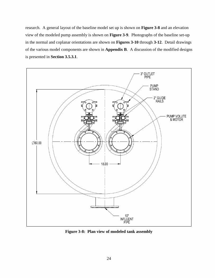
A flow loop, shown on Figure 3-13, was constructed in one of Alden Research Laboratory’s
Hydraulic Modeling Facilities. The loop utilized a 10 HP laboratory pump which withdrew water
from a 50,000-gallon sump. The flow was conveyed through one of three orifice plate flow meters
(2”, 4” or 6”), which was connected to the 10-inch influent piping by means of a manifold. Valves
located downstream of each meter were used to control the flow. The flow was measured with a
Differential Pressure (DP) cell and recorded with a computerized Data Acquisition (DA) System.
Flow entering each modeled pump bell was directed up through the acrylic pipe which housed the
swirl meter and down the “motor housing”, where it entered the volute and was carried out the 3-
inch effluent pipe. The outflow from each modeled pump was directed back to the laboratory
sump through a vertical return pipe, which was connected to the suction inlet of a 3 HP laboratory
centrifugal pump. Each pipe contained a 4-inch flow meter connected to a DP cell for measuring
the modeled pump flows. A 6-inch control valve on the discharge of each laboratory pump was
used to adjust the outflow.
A piezometer tap was connected to the wet well floor between the two modeled-pumps to measure
the water elevation within the tank. The elevation was measured and recorded with the use of a
DP cell and computerized DA system. An external stilling well and point gage were used as an
Modeled HI Recommendation
Bell Diameter (D) 7.5" Approximately 3"-8"
Bell Clearance (Cf) 2.92" 2.25"-3.75"
Wall Clearance (Cw) 13" 4" Minimum or 0.25D
Pump Volute Clearance (Cb) 2" 4" Minimum or 0.25D
Sump Diameter (Ds) 60" 44" Minimum
Parameter
28
established floor elevation reference. Detailed descriptions of the instrumentation used are found
in Section 3.4.2
Figure 3-13: Model setup and flow loop
3.4.2 Instrumentation and Measuring Techniques
3.4.2.1 Flow
The system inflow, as well as outflow from each modeled pump, was measured using orifice plate
meters, which consists of a restrictive plate sandwiched between two lengths of pipe. The meters
operate based on the Bernoulli’s Equation (energy equation) and continuity equation. The
differential pressure (head) can be related to the velocity in the pipe and hence, the flow.
Each meter was fabricated and installed per the American Society of Mechanical Engineers
(ASME) guidelines, as shown on Figure 3-14. Two pressure taps, oriented 180 degrees apart,
were located at a distance of 1D upstream and 1/2D downstream of the plate, where D is the inside
pipe diameter.

29
Figure 3-14: Guideline for fabrication of an orifice plate meter (ASME 2004)
Each meter contained a minimum of 20 pipe-diameters of straight pipe upstream and 5 diameters
of pipe downstream. The inflow meters, which were horizontal in orientation, contained bleed
valves in the crown of the pipes for evacuating air on the upstream side of the plate, as this will
affect the pressure reading and consequently, the accuracy of the flow reading. The differential
pressure from each flow meter was measured using a DP cell.
The flow from each meter was calculated using the standard orifice equation:
[9]
Where:
Q = flow, Cd = discharge coefficient, A0
ΔH = differential head across the orifice plate
= orifice area, g = gravity and
Cd relates actual flow to theoretical flow through a primary device.
30
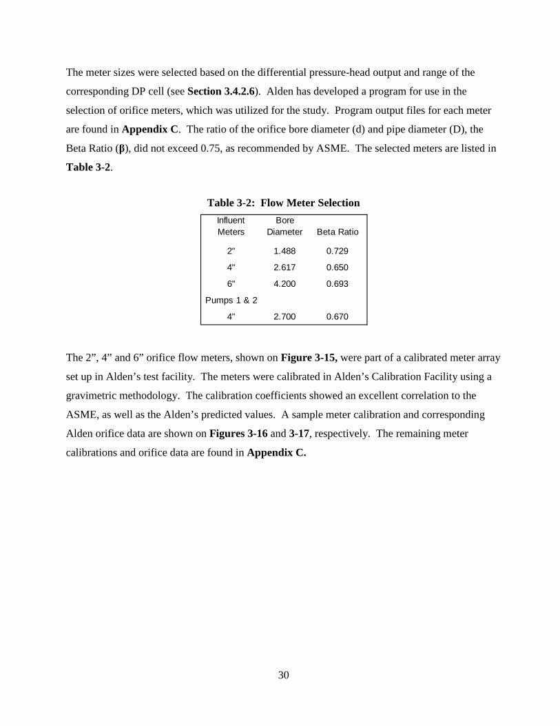
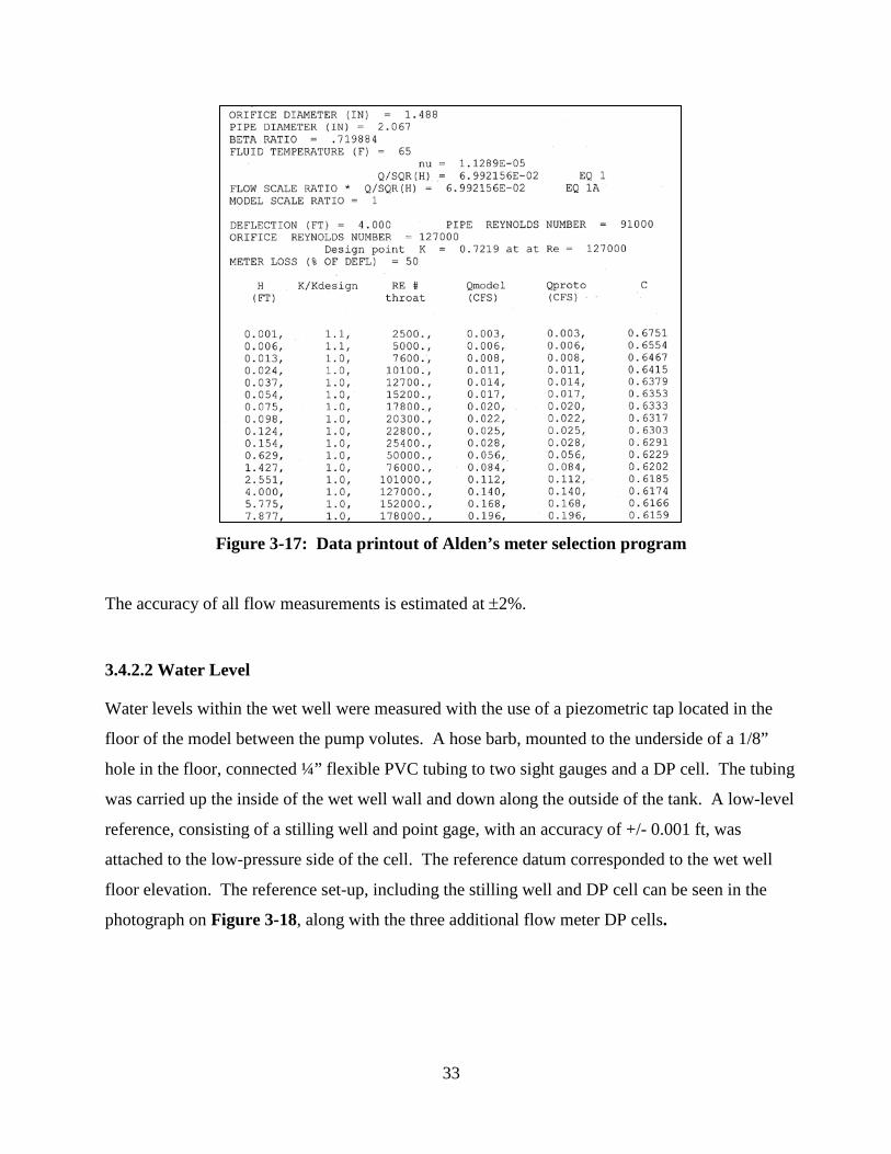
The meter sizes were selected based on the differential pressure-head output and range of the
corresponding DP cell (see Section 3.4.2.6). Alden has developed a program for use in the
selection of orifice meters, which was utilized for the study. Program output files for each meter
are found in Appendix C. The ratio of the orifice bore diameter (d) and pipe diameter (D), the
Beta Ratio (β), did not exceed 0.75, as recommended by ASME. The selected meters are listed in
Table 3-2.
Table 3-2: Flow Meter Selection
The 2”, 4” and 6” orifice flow meters, shown on Figure 3-15, were part of a calibrated meter array
set up in Alden’s test facility. The meters were calibrated in Alden’s Calibration Facility using a
gravimetric methodology. The calibration coefficients showed an excellent correlation to the
ASME, as well as the Alden’s predicted values. A sample meter calibration and corresponding
Alden orifice data are shown on Figures 3-16 and 3-17, respectively. The remaining meter
calibrations and orifice data are found in Appendix C.
Influent Meters
Bore Diameter Beta Ratio
2" 1.488 0.729
4" 2.617 0.650
6" 4.200 0.693
Pumps 1 & 2
4" 2.700 0.670
31
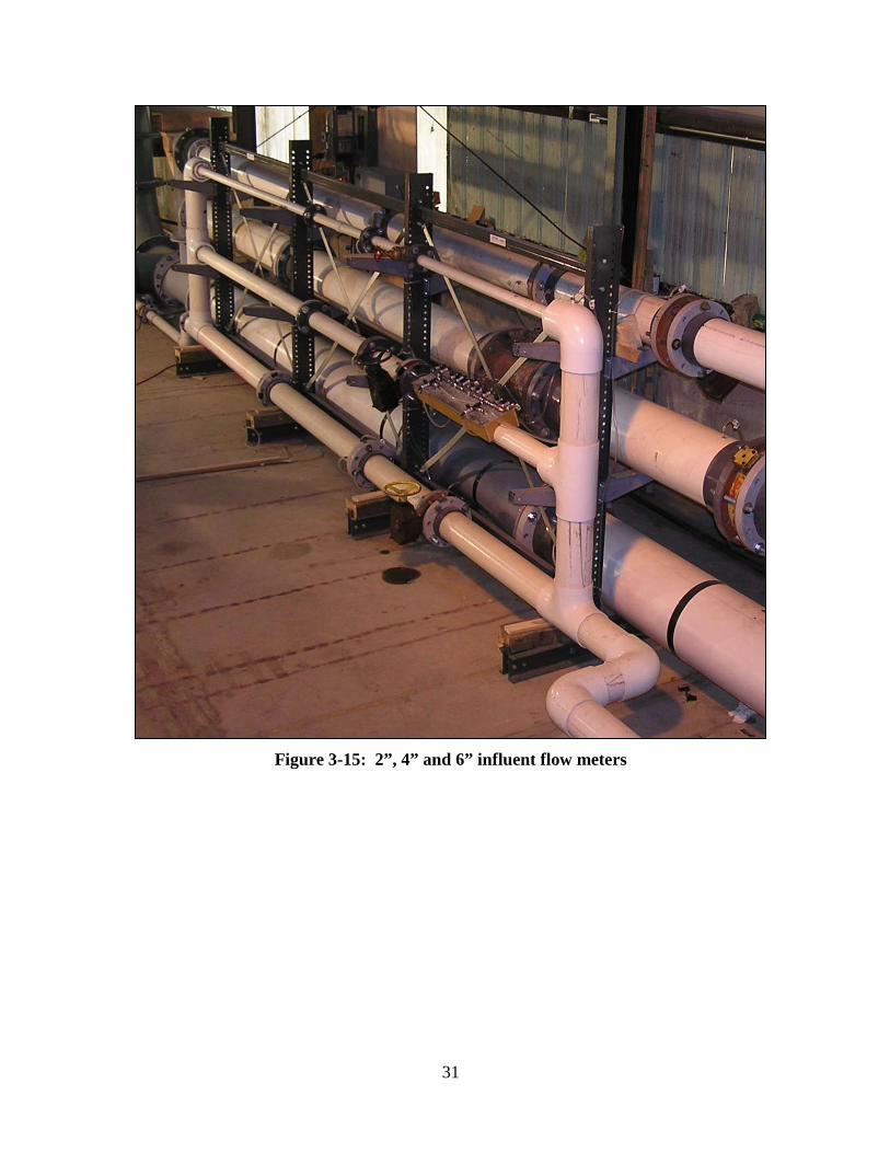
Figure 3-15: 2”, 4” and 6” influent flow meters

32
Figure 3-16: Calibration data of the 2-inch influent meter
33
Figure 3-17: Data printout of Alden’s meter selection program
The accuracy of all flow measurements is estimated at ±2%.
3.4.2.2 Water Level
Water levels within the wet well were measured with the use of a piezometric tap located in the
floor of the model between the pump volutes. A hose barb, mounted to the underside of a 1/8”
hole in the floor, connected ¼” flexible PVC tubing to two sight gauges and a DP cell. The tubing
was carried up the inside of the wet well wall and down along the outside of the tank. A low-level
reference, consisting of a stilling well and point gage, with an accuracy of +/- 0.001 ft, was
attached to the low-pressure side of the cell. The reference datum corresponded to the wet well
floor elevation. The reference set-up, including the stilling well and DP cell can be seen in the
photograph on Figure 3-18, along with the three additional flow meter DP cells.

34
Figure 3-18: Photograph of the water elevation DP cell (on left) and low-level
point-gage reference set up, along with the 3 flow meter DP cells.
3.4.2.3 Free Surface Vortices
The HIS has established a strength-scale for the formation of free-surface vortices which was used
in evaluating the hydraulic performance of the wet well. The scale, shown on Figure 3-19, ranges
from a Type 1 surface swirl, to a Type 6 open air-core to the suction inlet. Type 3 (dye-core) and
higher-strength vortices are deemed unacceptable by the HIS. Vortex types are identified in the
model by visual observations made with the use of dye (food coloring), wood chips, etc. during
steady-state conditions. Vortices of maximum strength are documented.

35
Figure 3-19: Free-surface vortex classification (Alden)
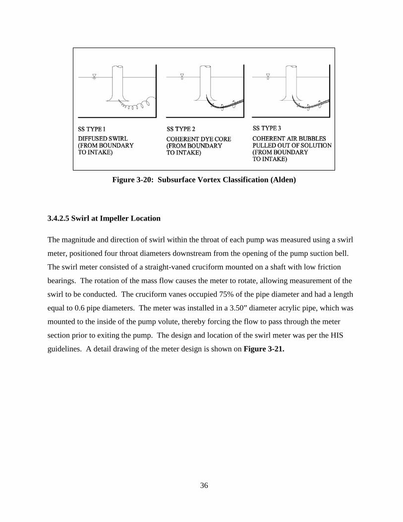
3.4.2.4 Subsurface Vortices
Subsurface vortices typically originate from surfaces that are normal and/or parallel to the pump
bells, such as the wet well floor and walls. Unlike free-surface vortices, the presence of
subsurface vortices may not be realized without the injection of dye. The HIS strength-scale for
the formation of subsurface vortices which was used in evaluating the hydraulic performance of
the wet well is shown on Figure 3-20. The scale ranges from a Type 1 helical shape to a Type 3
air-core. Air-cores are formed when the rotational velocity is high enough to cause a sufficient
low-pressure region within the core to release air bubbles from solution. Type 2 (dye-core) and
Type 3 vortices are deemed unacceptable by the HIS. Subsurface vortices were identified by
injecting dye on the floor beneath the suction bell of each pump. Dye was not introduced on the
wet well wall, as the pumps were of sufficient distance away to deter formation at that location.
36
Figure 3-20: Subsurface Vortex Classification (Alden)
3.4.2.5 Swirl at Impeller Location
The magnitude and direction of swirl within the throat of each pump was measured using a swirl
meter, positioned four throat diameters downstream from the opening of the pump suction bell.
The swirl meter consisted of a straight-vaned cruciform mounted on a shaft with low friction
bearings. The rotation of the mass flow causes the meter to rotate, allowing measurement of the
swirl to be conducted. The cruciform vanes occupied 75% of the pipe diameter and had a length
equal to 0.6 pipe diameters. The meter was installed in a 3.50” diameter acrylic pipe, which was
mounted to the inside of the pump volute, thereby forcing the flow to pass through the meter
section prior to exiting the pump. The design and location of the swirl meter was per the HIS
guidelines. A detail drawing of the meter design is shown on Figure 3-21.

37
Figure 3-21: Modeled swirl meter detail drawing
The rotation of the swirl meter was recorded and used to calculate a swirl angle, θ, which is an
indication of swirl intensity. This is performed by establishing the tangential function of the angle
produced by the ratio of the tangential velocity (Vt) and the axial velocity (u). Vt is determined by
correlating the revolutions per second (n) to the pipe circumference ( , thus producing a
velocity in feet per second. The axial velocity is the result of calculating Q/A for the swirl meter
pipe section, where Q = flow in cfs and A = area in ft2
[10]
. The swirl equation is written as:

38
where
u = axial velocity at the swirl meter location
d = diameter of the pipe at the swirl meter location
n = revolutions/second of the swirl meter
A graphical presentation of the swirl calculation is shown on Figure 3-22.
Figure 3-22: Relationship of axial to tangential velocity for swirl calculation (Alden)
Alden has developed instrumentation and programming to allow a computerized data acquisition
(DA) system to record the rotational direction and number of 1/2–revolutions of a swirl meter over
10-second time spans. This results in a higher accuracy in calculating the swirl angle over the
conventional method of counting the rotations of the meter manually. This is especially true for
conditions of high swirl, when it may be impossible to accurately count the rotations visually. In
those situations, the swirl would be deemed unacceptably high and modifications would be

39
developed. However, there may be situations where it is desirable to know the actual angle, such
as when performing comparative analyses.
Subsurface and free-surface vortices can induce pump swirl that is generally unsteady and
intermittent. Therefore, for each steady-state condition documented (Qin = Qout
The computerized DA system allowed for the development of a program which could
continuously record the swirl under dynamic conditions. The advantage of this is that real-time
data can be collected to evaluate the wet well while operating under realistic operating conditions.
In addition, this also allows us to evaluate the level of conservation of collecting data under
steady-state conditions for systems that typically operate dynamically. Since the development of
the Alden instrumentation and programming is deemed proprietary, the details cannot be discussed
in this paper.
for a constant
water elevation), the number of half revolutions and direction of rotation of each swirl meter was
obtained over twenty 30-second intervals, covering a period of 10 minutes. The total counts for
each interval are determined by adding the clockwise and counterclockwise counts. From these
data, the absolute 30-second maximum and 10-minute average swirl angle was obtained in
accordance to the HIS guidelines for swirl. Although the wet well operates dynamically,
collecting the steady state data allowed for a comparative analysis of designs, which could be
correlated to the HIS acceptance criteria.
3.4.2.6 Differential Pressure Cells
As the name implies, Differential Pressure (DP) cells were utilized for the measurement of the ΔP
generated from the flow meters and water level-to-reference Piezometer tap. The cells,
manufactured by Rosemount®, measured the differential between a high and low-pressure source
and converted it to an electrical output ranging from 2 to 10 mV. These values were then used as
inputs into the computer programs in conjunction with the corresponding calibrations, to output
water elevation and flow data. The cells, shown on Figure 3-18, were plumbed together by
connecting all the high and low input lines. This allowed for ease in bleeding the air out of the
cells at the start of each testing session.

40
Each DP cell was calibrated prior to use in the model. This was achieved by setting a series of
known deflections on a standard 8-foot high water manometer board and recording the voltages
for each cell. All the cells were calibrated simultaneously through the use of the connected inputs.
A minimum of 5 points were used to cover each cell range and establish the corresponding slopes
and intercepts. The cells were connected to the computer through the use of an Analog-to-Digital
(A/D) board. The calibration of the influent flow cell is shown on Figure 3-23. All calibration
data is shown in Appendix C.
Figure 3-23: Influent flow DP cell calibration
3.4.2.7 Computer Data Acquisition and Analysis Programs
Various computer programs were utilized for acquiring test data and performing data analysis.
Initial testing, conducted under steady state conditions, required two programs and computers for
completion. A LABVIEW data acquisition program, written by Alden Research, was used for
measuring the inflow, modeled pump flow(s) and water elevation within the wet well. The
program utilized the DP cell calibrations and flow meter coefficients to record to file and output to
screen, flow (in gpm) and water elevation (in feet). The program output files were in an X.DAT
format, which were imported into an EXCEL spreadsheet for post processing. The sampling rate
for data collection was 100 Hz, with readings averaged every 5 seconds throughout the duration of
the test. Steady state swirl readings, discussed in Section 3.4.2.5, were recorded by a second
computer with the use of a machine code program developed at Alden. The program recorded
Influent Channel #0
Delta-H Delta-H Delta-H 0-72"inch ft psi Volts
0 0.000 0.000 2.0413.75 0.313 0.135 2.477.12 0.593 0.257 2.85916.68 1.390 0.602 3.9426.56 2.213 0.958 5.0837.53 3.128 1.354 6.33146.86 3.905 1.691 7.39857.02 4.752 2.057 8.55465.63 5.469 2.368 9.541
y = 0.3157x - 0.6444R² = 1
0.0
0.3
0.6
0.9
1.2
1.5
1.00 2.00 3.00 4.00 5.00 6.00 7.00 8.00
Del
ta-H
(psi
)
Volts
Channel #0 DP Cell - Influent
41
swirl meter rotations in ½ turn increments over periods of 10 seconds, for duration of 10 minutes,
thereby allowing for 10 or 30-second maximum and 10-minute averages to be reported as per the
HIS criteria. The program output files were in an X.DAT format, which were imported into an
EXCEL spreadsheet for final processing.
As testing progressed, it was realized that steady state data might not be representative of the
actual swirl conditions experienced under normal dynamic operating conditions. Therefore, the
model instrumentation and programming was changed to allow the recording of real-time flow,
swirl and water elevations. A LABVIEW program was written by Alden personnel, which could
record pulses of 0mv, 1mv or 5mv from the swirl meter as it rotated in ¼-turn increments. The
program and new interface enabled for the documentation of both intensity and direction of swirl.
The sampling rate of the program was set to 250 Hz. The duration of data recording was an input
variable selected in 1-second cycles. The output of the dynamic data files were in an X.BIN
format.
An OCTAVE program was used to process the raw dynamic data. The program analyzed the
recorded pulses and determined when a full rotation of the swirl meter occurred. Although a finer
resolution of swirl angle was possible, the additional data points made the graphs hard to analyze.
The timestamp of the data allowed for the calculation of revolutions/sec to be determined, which
was then used to determine the swirl angle, as described in Section 3.4.2.5. Swirl direction was
determined by analyzing the order of the pulses and a designation of (+) (CCW) or (-) (CW) was
assigned to the value.
3.5 PHYSICAL MODEL TEST PROGRAM
3.5.1 HIS Acceptance Criteria
The evaluation of the hydraulic performance of the wet well was conducted according to the HIS
acceptance criteria for pump intakes, as listed below. Under this criterion, free-surface vortices,
subsurface vortices and swirl angles were measured, while operating the model under steady state
conditions. There is also a requirement for velocity measurements in the pump suction throat.
However, this criterion omitted from this stage of the research, as it applies to a selected final
design. Although this may be included in future testing, it has been observed that designs

42
satisfying the HIS acceptance criteria for vortex severities and swirl generally achieve acceptable
velocity distribution at the suction throat if not immediately preceded by an elbow..
The HIS acceptance criteria are as follows:
Parameter
Free Surface Vortices Type 1 or 2
Maximum Acceptable Values
Type 3 < 10% of time or for infrequent pump operating conditions. See Figure 3-19 for classification.
Subsurface Vortices Type 1 Type 2 < 10% of time or for infrequent pump operating conditions. See Figure 3-20 for classification.
Swirl Angles 10-30 second maximum and 10 minute average <5 degrees 10-30 second maximum up to 7 degrees, if occurring < 10% of time
or for infrequent pump operating conditions. The meter should not experience sudden changes in direction when rotating near the allowable rate.
Each test also included general observations of wet well flow patterns, as well as any air-
entrainment into the pumps, due to the influences of the selected inflow and water elevation.
Clean out performance tests for scum removal were conducted during the evaluation of the
modified design. Discussion of the methodology is found in Section 3.5.3.
3.5.2 Baseline Geometry and Testing Methodology
3.5.2.1 Baseline Geometry
The baseline geometry consisted of an open wet well (no fillet) and standard pump installation
with no cones, as described in Sections 3.2.1 and 3.4.1. The wet well initially consisted of only
the lower section of the tank and therefore, had an available height of 4 feet. The normal and
coplanar orientations were tested, with both one-pump and two pumps operating. Although the
geometry is not conducive for solids removal, the data obtained can be applied to clear liquid
pumping applications.

43
3.5.2.2 Testing Methodology
Testing was initiated at a water elevation of approximately 3.5 feet. The inflow was set slightly
lower than the pump flow, resulting in a steady drawdown of the water elevation at a rate of
approximately -0.016 ft/minute. Free surface and subsurface vortices were documented through
the duration of drawdown. Pump swirl was recorded under steady-state conditions at elevations of
approximately 3.5 feet and 1.42 feet, corresponding to an intermediate water level (IWL) and low
water level (LWL).
The normal and coplanar orientation baseline conditions was retested after the completion of the
modified design testing in order to obtain dynamic test data for the no-flow, 25 gpm and 125 gpm
influent conditions. The testing was performed with the upper riser installed, allowing for the
testing to be initiated at a water elevation of 6 feet. Performing these tests allowed for a better
understanding of the impact of the modifications on pump swirl under dynamic operating
conditions.
Video documentation of free surface and subsurface vortices was conducted for selected operating
conditions.
3.5.3 Modified Geometry and Testing Methodology
3.5.3.1 Modified Geometry
In order to evaluate the hydraulic conditions in the wet well under solid-bearing liquid operating
conditions, the baseline geometry was modified by adding a 45-degree sidewall fillet and 90-
degree pump cones (to eliminate subsurface vortices), as described in Sections 3.2.2 and 3.4.1.
The pump cones were fabricated from solid acrylic. The fillet was fabricated from 0.08-inch
acrylic sheet. The fillet shape was achieved by installing support ribs to the wet well floor and
fastening the sheets to the ribs. The toe of each sheet was fastened to a continuous floor cleat to
maintain the shape at the pumps. The height of the fillet was not continuous around the perimeter
of the wet well. Because of this, the full diameter of the inlet pipe intersected the fillet face for the
normal orientation, while only the bottom of the pipe intersected it for the coplanar orientation.
The inlet pipe was extended for the normal orientation by inserting an acrylic sleeve into the

44
existing pipe. The shape of the outside diameter was cut out of the fillet face and the seams were
sealed. A crescent piece of pipe was fitted between the existing pipe and fillet for the coplanar
design. Each unused cut-out was blocked during testing. A layout of the ribs and floor cleat is
shown on Figure 3-24. A photograph of one of the pump cones is shown on Figure 3-25.
Photographs of the modified geometry in the normal and coplanar orientations are shown on
Figures 3-26 and 3-27, respectively.
Figure 3-24: Layout of fillet support ribs and floor cleat

45
.
Figure 3-25: Photograph of typical pump cone
Figure 3-26: Modified wet well geometry in the normal orientation

46
Figure 3-27: Modified wet well geometry in the coplanar orientation
3.5.3.2 Testing Methodology
Testing was conducted under both steady state and dynamic operating conditions. A 3-ft high
riser section was added to the model tank to allow for testing to be initiated at a high-water
elevation of 6 ft, to better understand the hydraulic performance of the wet well. The scope of
testing for the steady state conditions was similar to that of the baseline testing. Swirl data and
vortices were recorded under steady state conditions at 1-foot, 6-inch and 3-inch intervals as the
water level was sequentially lowered. The swirl data was recorded so that a minimum operating
water level, based on acceptable swirl, could be established.
Dynamic testing was conducted on each pump for both inlet orientations. The target inflow was
set and the tank allowed to fill. The elevation was stabilized at approximately 6 ft by balancing
the inflow with the outflow of the tested pump. The data recording was then initiated and the
modeled pump flow was increased to 250 gpm. The test was terminated after the test pump broke
siphon due to air entrainment.
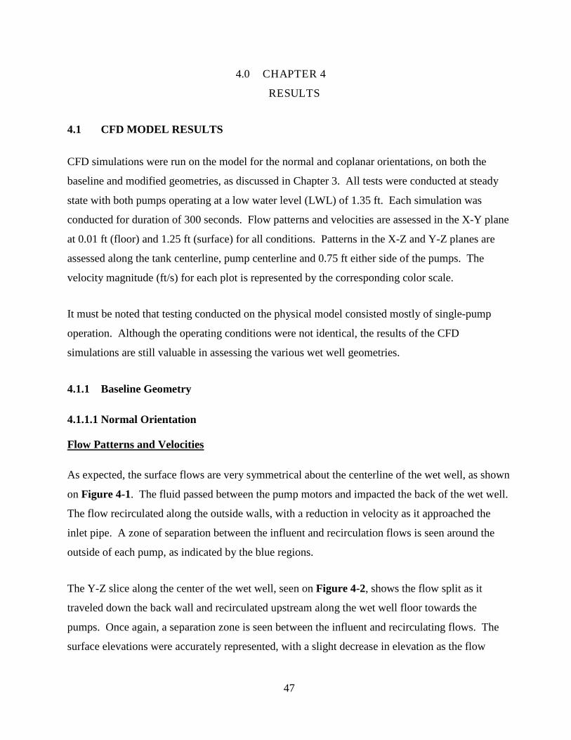
47
4.0 CHAPTER 4
RESULTS
4.1 CFD MODEL RESULTS
CFD simulations were run on the model for the normal and coplanar orientations, on both the
baseline and modified geometries, as discussed in Chapter 3. All tests were conducted at steady
state with both pumps operating at a low water level (LWL) of 1.35 ft. Each simulation was
conducted for duration of 300 seconds. Flow patterns and velocities are assessed in the X-Y plane
at 0.01 ft (floor) and 1.25 ft (surface) for all conditions. Patterns in the X-Z and Y-Z planes are
assessed along the tank centerline, pump centerline and 0.75 ft either side of the pumps. The
velocity magnitude (ft/s) for each plot is represented by the corresponding color scale.
It must be noted that testing conducted on the physical model consisted mostly of single-pump
operation. Although the operating conditions were not identical, the results of the CFD
simulations are still valuable in assessing the various wet well geometries.
4.1.1 Baseline Geometry
4.1.1.1 Normal Orientation
As expected, the surface flows are very symmetrical about the centerline of the wet well, as shown
on Figure 4-1. The fluid passed between the pump motors and impacted the back of the wet well.
The flow recirculated along the outside walls, with a reduction in velocity as it approached the
inlet pipe. A zone of separation between the influent and recirculation flows is seen around the
outside of each pump, as indicated by the blue regions.
Flow Patterns and Velocities
The Y-Z slice along the center of the wet well, seen on Figure 4-2, shows the flow split as it
traveled down the back wall and recirculated upstream along the wet well floor towards the
pumps. Once again, a separation zone is seen between the influent and recirculating flows. The
surface elevations were accurately represented, with a slight decrease in elevation as the flow

48
passed between the pump motors and a welling-up of the surface as the flow impacted the back
wall.
Figure 4-1: Near-surface flow patterns and velocity magnitudes (ft/s)
At Elevation 1.25 ft (flow = 250 gpm/pump)

49
Figure 4-2: Wet well centerline flow patterns and velocity magnitudes (ft/s)
(flow = 250 gpm/pump)
Flow along the wet well floor, as seen on Figure 4-3, was fairly symmetrical about the centerline
of the wet well, with equal recirculation along the outside walls and reduced velocity as it
approached the upstream end of the wet well. The velocity was relatively high as the flow passed
between the pump stands. Regions of separation and low-velocity can be seen around the outside
of the stands and under the inlet pipe. The appearance of non-symmetry around the pump stands
was probably due to the blockage caused by the pump volutes, which are non-symmetrical in
design. It is interesting to note that the direction of swirl entering the pumps is directly related to
the flow approaching the bells from between the pump stands and not the overall circulation
direction within the wet well, as what one would expect.

50
Figure 4-3: Floor flow patterns and velocity magnitudes (ft/s)
At Elevation 0.01 ft (flow = 250 gpm/pump)
Figures 4-4, 4-5 and 4-6 show the flow patterns and velocity magnitudes upstream, on-center and
downstream of the pumps, as viewed from upstream to downstream. The figures clearly show the
flow direction along the wet well walls and influence of the pumps and stands on overall flow
patterns. Although the flow patterns within the wet well are not defined in figure 4-5 due to the
velocity scale, the boundary regions caused by the various flow patterns can be seen.
Inflow

51
Figure 4-4: Flow patterns and velocity magnitudes (ft/s)
0.75 ft upstream of pumps (flow = 250 gpm/pump)
Figure 4-5: Flow patterns and velocity magnitudes (ft/s) along pump centerlines
(flow = 250 gpm/pump)

52
Figure 4-6: Flow patterns and velocity magnitudes (ft/s)
0.75 ft downstream of pumps (flow = 250 gpm/pump)
4.1.1.2 Coplanar Orientation
Figures 4-7 and 4-8 show the flow impacting and diverting around either side of the upstream
pump. The flow patterns within the wet well were not symmetrical, due to the blockage of the
guide rails and outlet pipes, which creates a channel of higher velocity on the stand side of the
pumps. A surface depression with an indication of an air interface is seen on the downstream side
of pump 1 and is represented by the white coloration.
Flow Patterns and Velocities
The flow patterns along the floor, as seen on Figure 4-9, show numerous regions of flow
separation, due to the asymmetry of the flow within the wet well. The approach flow to pump 1
was mainly from the stand side of the pump. The upstream pump-stand created a separation of
flow, with high velocity being forced to the surface and lower velocity flow downward to the bell
of the pump, as seen on Figure 4-10. This resulted in a clockwise rotation (as viewed from the
top) of the flow entering the pump. Flow approached pump 2 from the open side of the wet well,
resulting in a counterclockwise rotation. As can be seen on Figure 4-11, the flow had a
downward trajectory as it was being drawn into the pump on the open side. The velocity around
the pump bell was higher at pump 2, with the area of circulation being larger and more uniform

53
than pump 1. Figure 4-12 shows the high surface flow on the pump-stand side of the wet well
(right side) and downward flow on the open side.
Figure 4-7: Near-surface flow patterns and velocity magnitudes (ft/s)
At Elevation 1.25 ft (flow = 250 gpm/pump)

54
Figure 4-8: Wet well centerline flow patterns and velocity magnitudes (ft/s)
(flow = 250 gpm/pump)
Figure 4-9: Floor flow patterns and velocity magnitudes (ft/s)
At Elevation 0.01ft (flow = 250 gpm/pump)
Inflow

55
Figure 4-10: Flow patterns and velocity magnitudes (ft/s)
0.75 ft near side of pumps (flow = 250 gpm/pump)
Figure 4-11: Flow patterns and velocity magnitudes (ft/s)
0.75 ft far side of pumps (flow = 250 gpm/pump)
Inflow
Inflow

56
Figure 4-12: Flow patterns and velocity magnitudes (ft/s) between pumps
(looking upstream, flow = 250 gpm/pump)
4.1.1.3 Baseline Summary
The normal orientation produced symmetrical flow patterns within the wet well. There was a
separation in direction of circulation between the flow at the surface and wet well floor. This was
due to the downward flow along the back wall which was redirected upstream along the center of
the tank, as opposed to the outside wall. There were regions of well-defined flow circulation
under each pump bell, in counter-rotating directions. The velocities under the bells were
approximately 1 ft/s to 1.5 ft/s in magnitude.
As expected, the coplanar orientation produced very different flow patterns due to the obstruction
caused by the upstream pump. The split to either side of the pump however, was not uniform, due
to the added obstruction from the pump stands. This resulted in higher surface velocities of
approximately 2 ft/s to 2.5 ft/s on the left side of the pump (looking downstream) and general
clockwise rotation in the tank. The surface velocity on the unobstructed side of the tank was
generally 1 ft/s or less. The floor velocities were higher on the unobstructed side with less regions
of separation than seen around the pump stands. There were well-defined regions of circulation
under each pump, with the direction of rotation at pump 1 being clockwise and pump 2
counterclockwise. The rotational velocity was higher at pump 2, with a magnitude of
approximately 3 ft/s, while pump 1 had about 1.5 ft/s.

57
Since both designs produced well-defined regions of rotation under the pumps, it cannot clearly be
stated that one design is advantageous over the other. Both showed conditions which could
potentially lead to the development of subsurface vortices and/or high pump swirl.
4.1.2 Modified Geometry
4.1.2.1 Normal Orientation
With the installation of the 45-degree fillet, the volume of the available wet well was greatly
reduced. This resulted in a greater amount of surface turbulence and fluctuation of water surface
elevation, as seen on Figure 4-13 (indicated by the white regions) and Figure 4-14. The surface
flow patterns did not have the same level of symmetry as in the baseline condition. This was
probably due to the air interface regions caused by the turbulence, as well as the higher influence
of the pump volute shape on the flow patterns, since the blockage to open-volume ratio was much
greater. The inflow followed the upstream fillet slope down to the floor. However, this most
likely represents the wet well recirculation flow, as the fluid would not expand along the 45-
degree slope without the presence of a headloss device. It can be seen that the flow travelled up
the back slope, with no indication of separation, as in the baseline condition.
Flow Patterns and Velocities

58
Figure 4-13: Near-surface flow patterns and velocity magnitudes (ft/s)
At Elevation 1.25 ft (flow = 250 gpm/pump)
Air due to surface turbulence

59
Figure 4-14: Wet well centerline flow patterns and velocity magnitudes (ft/s)
(flow = 250 gpm/pump)
The lack of separation along the back slope resulted in the flow maintaining a constant rotational
direction around each pump. This is evident when viewing the flow patterns on Figure 4-15, as
the direction of rotation is the same at the floor as at the surface. With a reduced floor area under
the pumps, the velocity under the bells was approximately 3.5 ft/s, double that of the baseline
condition, which is advantageous for solids removal. However, the rotation around the bells was
more defined, which could indicate the presence of higher swirl and/or stronger subsurface
vortices depending on the magnitude of the turbulence.
Figure 4-15: Floor flow patterns and velocity magnitudes (ft/s)
At Elevation 0.01 ft (flow = 250 gpm/pump)
Inflow

60
Continuity of the flow and symmetry of the overall patterns can be seen on Figures 4-16 through
4-18. There were no regions of separation caused by varying flow directions as in the baseline
condition. However, the flow separation caused by the blockage of the pump stands was greater
than the previous condition. The bottom of the wet well shown on Figures 4-16 and 4-18 appear
to be rounded in design. This is due to position of the plot slices, which are located part way up
the front and back slopes.
Figure 4-16: Flow patterns and velocity magnitudes (ft/s)
0.75 ft upstream of pumps (flow = 250 gpm/pump)
Figure 4-17: Flow patterns and velocity magnitudes (ft/s) along the pump centerlines
(flow = 250 gpm/pump)
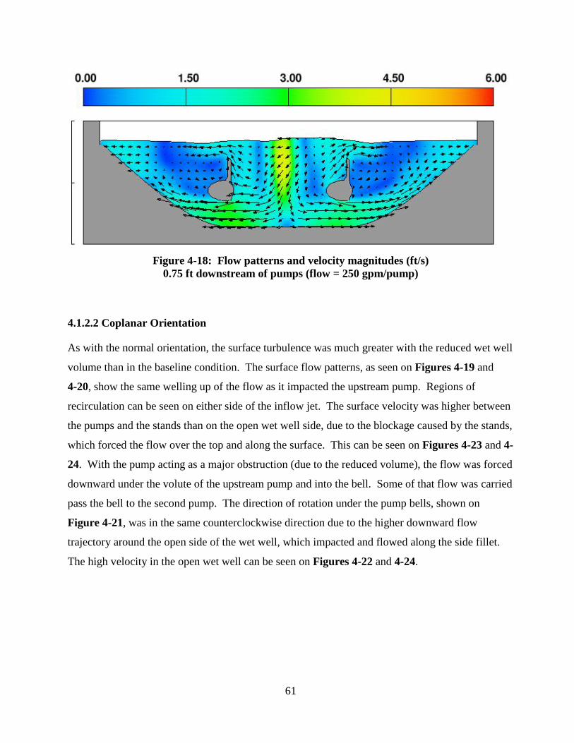
61
Figure 4-18: Flow patterns and velocity magnitudes (ft/s)
0.75 ft downstream of pumps (flow = 250 gpm/pump)
4.1.2.2 Coplanar Orientation
As with the normal orientation, the surface turbulence was much greater with the reduced wet well
volume than in the baseline condition. The surface flow patterns, as seen on Figures 4-19 and
4-20, show the same welling up of the flow as it impacted the upstream pump. Regions of
recirculation can be seen on either side of the inflow jet. The surface velocity was higher between
the pumps and the stands than on the open wet well side, due to the blockage caused by the stands,
which forced the flow over the top and along the surface. This can be seen on Figures 4-23 and 4-
24. With the pump acting as a major obstruction (due to the reduced volume), the flow was forced
downward under the volute of the upstream pump and into the bell. Some of that flow was carried
pass the bell to the second pump. The direction of rotation under the pump bells, shown on
Figure 4-21, was in the same counterclockwise direction due to the higher downward flow
trajectory around the open side of the wet well, which impacted and flowed along the side fillet.
The high velocity in the open wet well can be seen on Figures 4-22 and 4-24.

62
Figure 4-19: Near-surface flow patterns and velocity magnitudes
At Elevation 1.25 ft (flow = 250 gpm/pump)
Figure 4-20: Wet well centerline flow patterns and velocity magnitudes (ft/s)
(flow = 250 gpm/pump)

63
Figure 4-21: Floor flow patterns and velocity magnitudes (ft/s)
At Elevation 0.01 ft (flow = 250 gpm/pump)
Figure 4-22: Flow patterns and velocity magnitudes (ft/s)
0.75 ft near side of pumps (flow = 250 gpm/pump)
Inflow
Inflow

64
Figure 4-23: Floor flow patterns and velocity magnitudes (ft/s)
0.75 ft far side of pumps (flow = 250 gpm/pump)
Figure 4-24: Flow patterns and velocity magnitudes (ft/s) between pumps
(looking upstream, flow = 250 gpm/pump)
4.1.2.3 Modified Design Summary
The normal orientation maintained a constant counter-rotational direction of flow around each
pump throughout the depth of the wet well. The 45-degree fillet prevented the flow separation at
the back wall experienced with the baseline condition. The reduction in wet well volume resulted
in higher surface turbulence and fluctuation of the surface profile as indicated by the white regions
Inflow

65
on Figure 4-13. The direction of circulation under the pumps was opposite that of the baseline
condition, but still maintained counter-rotational directions. The rotational velocity under the
pumps was approximately 4 ft/s, which was 3 to 4 times higher than the baseline condition.
The coplanar design showed similar results to that of the baseline conditions, with higher surface
velocities on the pump-stand side of the pumps and a tendency for the flow to project downward
on the open side of the wet well. The direction of rotation under the bell was counterclockwise for
both pumps, which was different from the baseline condition. Pump 1 experienced the highest
rotational velocity with a magnitude of approximately 2.7 ft/s, compared to about 2 ft/s for pump
2.
Although the coplanar orientation produced lower rotational velocities than the normal orientation,
the circulation patterns are still well defined, indicating the possibility of the formation of
subsurface vortices and/or unacceptable pump swirl, depending on the level of turbulence. Once
again, the CFD results did not indicate that one design was advantageous over the other.
4.2 PHYSICAL MODEL RESULTS
Physical testing on the model was conducted for the normal and coplanar orientations, on both the
baseline and modified geometries, as discussed in Chapter 3 and presented in the following
sections. Tests were conducted at both steady state and dynamic operating conditions, with one
and two pumps operating. The steady state testing presented in Section 4.2.1, included
documentation of free and subsurface vortices, flow patterns and pump swirl. Dynamic testing
presented in Section 4.2.2, included documentation of swirl and free-surface vortices. Clean-out
tests were conducted for the 45-degree fillet design with the normal orientation only and results
are discussed in Section 4.2.2.2.4. Since the pumping stations are designed for 1-pump operation,
the 2-pump operation was only tested at low water elevation, to allow for a comparative analysis
between the CFD and physical model.
For the duration of this document, counterclockwise rotation will be designated as CCW and
clockwise rotation as CW.

66
The repeatability of the recorded steady state pump swirl presented in Sections 4.2.1.1 and 4.2.1.2
(10-minute average and 30-second maximum) was addressed by conducting back-to-back swirl
tests for selected water elevations. The test results, shown in Table 4-1, compares the averages to
the test results and shows the highest deviation rounded up to the nearest 0.5 degrees. The
maximum deviation shown is +/- 1-degree for the unsteady flow conditions experienced at LWL.
Steady State Swirl Repeatability
Table 4-1: Steady State Swirl Repeatability Data
4.2.1 Steady State Testing
In order to assess the performance of the station in accordance with the HI acceptance criteria for
swirl and vortex strength, the model testing was conducted at steady state operating conditions,
where Qin = Qout
at a selected elevation..
+ / -Degrees
1.42 10 min avg. 12.130 sec Max. 18.4
1.42 10 min avg. 13.2 10 min avg. 12.4 130 sec Max. 19.2 30 sec Max. 18.3 1
1.42 10 min avg. 11.930 sec Max. 17.4
2.25 10 min avg. 2.830 sec Max. 5.2
2.25 10 min avg. 3.2 10 min avg. 2.8 0.530 sec Max. 5.8 30 sec Max. 5.1 1
2.25 10 min avg. 2.430 sec Max. 4.2
2.5 10 min avg. 2.830 sec Max. 5.1
2.5 10 min avg. 2.4 10 min avg. 2.5 0.530 sec Max. 5.1 30 sec Max. 4.8 1
2.5 10 min avg. 2.230 sec Max. 4.1
6 10 min avg. 2.730 sec Max. 4 10 min avg. 2.7 0.5
6 10 min avg. 2.6 30 sec Max. 3.7 0.530 sec Max. 3.4
Water Elevation (ft)
Indicated Pump Swirl Averages

67
4.2.1.1 Baseline Geometry
4.2.1.1.1 Normal Orientation
The flow patterns within the wet well during the 2-pump operation matched the predicted patterns
of the CFD simulation at the low water level. The flow separated at the back wall and moved
down to the floor, where it passed between the pump stands and approached the pumps from the
downstream side. The surface flow recirculated around the outside wall of the wet well. The
rotational direction of the pump flow, as indicated by the swirl meters, was opposite that of the
surface flow, as in the CFD results.
Flow patterns
The 1-pump operating conditions gave similar results in overall flow patterns, but with much less
symmetry than the 2-pump test. The flow was skewed towards the operating pump, especially
along the wet well floor. The surface flow patterns were essentially the same as with the 2-pump
condition, as this is more dependent on the wet well shape than on pump operation.
Air bubbles could be seen entering the wet well during the open-channel influent flow conditions,
due to the close proximity of the hydraulic jump in the influent pipe. The air bubbles did not enter
the pumps until the water level dropped low enough to allow the jump to enter the wet well for the
2-pump condition. The surface energy was high during the open-channel operating conditions due
to the critical and supercritical (as the elevation dropped) influent flow. The energy dissipated
once the water level reached the crown of the pipe and the surface was quiescent at higher
elevations.
As expected, the surface energy and air concentration was much less at the 1-pump operating
conditions. Air bubbles were not observed entering the operating pump until the water level
dropped well below the invert of the pipe, creating a free-discharging condition and impingement
of air below the surface.
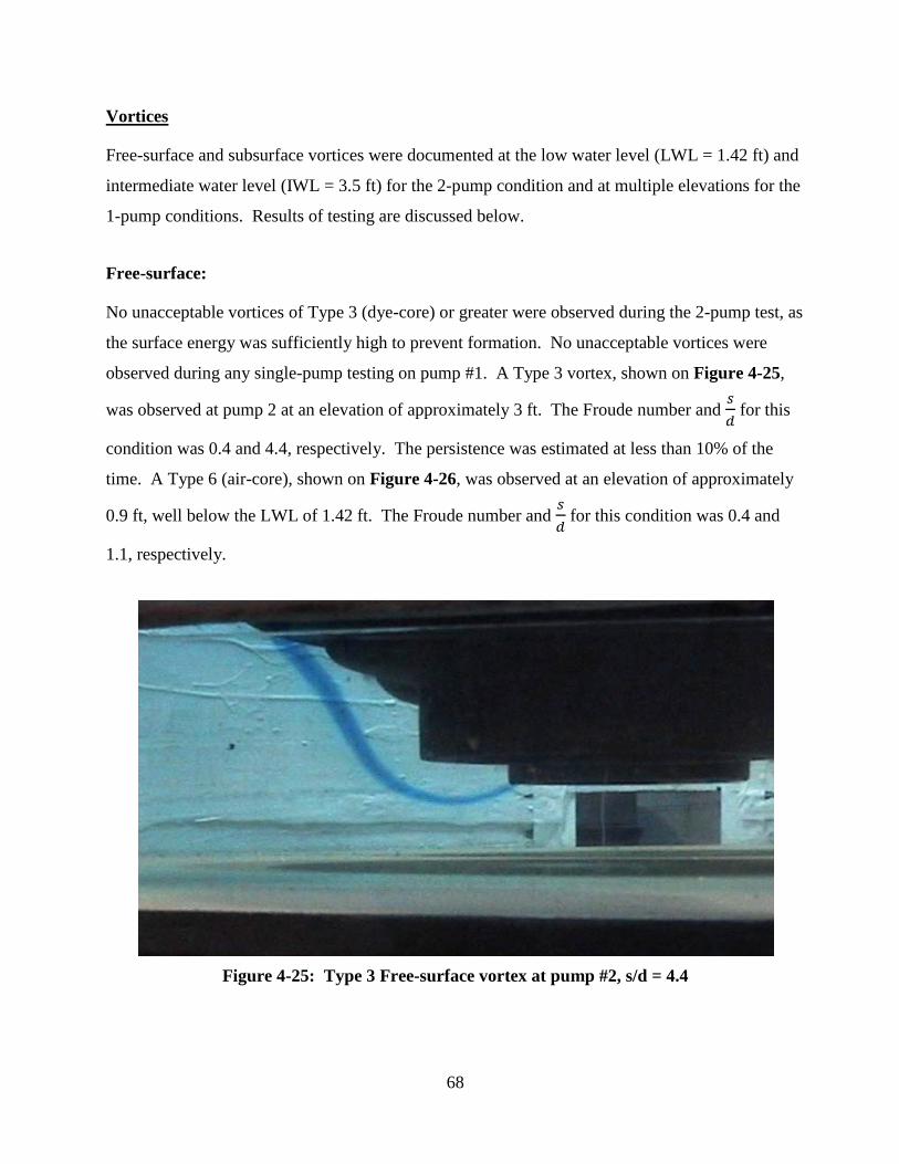
68
Vortices
Free-surface and subsurface vortices were documented at the low water level (LWL = 1.42 ft) and
intermediate water level (IWL = 3.5 ft) for the 2-pump condition and at multiple elevations for the
1-pump conditions. Results of testing are discussed below.
Free-surface:
No unacceptable vortices of Type 3 (dye-core) or greater were observed during the 2-pump test, as
the surface energy was sufficiently high to prevent formation. No unacceptable vortices were
observed during any single-pump testing on pump #1. A Type 3 vortex, shown on Figure 4-25,
was observed at pump 2 at an elevation of approximately 3 ft. The Froude number and for this
condition was 0.4 and 4.4, respectively. The persistence was estimated at less than 10% of the
time. A Type 6 (air-core), shown on Figure 4-26, was observed at an elevation of approximately
0.9 ft, well below the LWL of 1.42 ft. The Froude number and for this condition was 0.4 and
1.1, respectively.
Figure 4-25: Type 3 Free-surface vortex at pump #2, s/d = 4.4

69
Figure 4-26: Type 6 Free-surface vortex at pump #2, s/d = 1.1
Subsurface:
Type 2 (dye-core) vortices were present under all operating pumps, regardless of water elevation,
for the initial documented tests. It was observed that the persistence decreased with increasing
water elevation; however, the exact persistence rate is unknown. Type 3 (air-core) vortices were
observed during the 2-pump LWL test. Photographic documentation of the vortices is shown on
Figure 4-27. Type 3 vortices were also observed under each pump during the 1-pump tests for all
elevations below 3.5 ft. The strength and persistence increased with decreasing elevation for both
pumps and approached 100% at LWL.
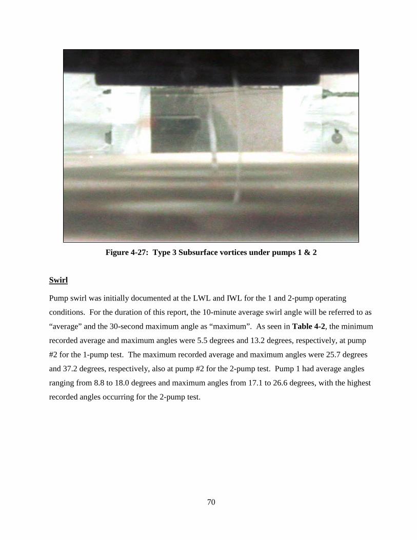
70
Figure 4-27: Type 3 Subsurface vortices under pumps 1 & 2
Swirl
Pump swirl was initially documented at the LWL and IWL for the 1 and 2-pump operating
conditions. For the duration of this report, the 10-minute average swirl angle will be referred to as
“average” and the 30-second maximum angle as “maximum”. As seen in Table 4-2, the minimum
recorded average and maximum angles were 5.5 degrees and 13.2 degrees, respectively, at pump
#2 for the 1-pump test. The maximum recorded average and maximum angles were 25.7 degrees
and 37.2 degrees, respectively, also at pump #2 for the 2-pump test. Pump 1 had average angles
ranging from 8.8 to 18.0 degrees and maximum angles from 17.1 to 26.6 degrees, with the highest
recorded angles occurring for the 2-pump test.

71
Table 4-2: Initial Recorded Swirl Angles At Low and Intermediate Water Levels Normal Orientation, Baseline Geometry
The addition of the top tank riser section made it possible to assess the swirl angles at high water
levels. Subsequent tests were performed for the 1-pump operating conditions at 6, 5 and 4-ft
elevations. Intermediate tests were also added at 3, 2.5 and 2-ft elevations to establish the overall
curves.
As seen in Table 4-3, the average swirl angles for pump #1 were approximately one-half the
magnitude of the maximum angles for all tests conducted. The swirl angles were lowest at the
higher elevations and gradually increased with decreasing water level, with the highest average
and maximum values of 13.8 and 22 degrees, respectively, being recorded at elevation 3.01 ft.
Surprisingly, the lowest average and maximum values of 2.4 and 4.0 degrees, respectively, were
recorded at elevation 5.07 ft and not at the highest elevation of 6 ft, which had swirl angles of 3.2
and 7.1 degrees. A sudden drop in swirl angle was recorded at elevation 2.5 ft, which produced
average and maximum angles of 4.5 and 9.9 degrees, respectively. The direction of swirl was
primarily CCW until the water level dropped below the crown of the influent pipe, when it
switched to a CW direction. In general, all tests, with the exception of the 5-ft elevation, produced
unacceptable swirl angles in accordance with the HI acceptance criteria. A graphical
representation of the swirl is shown on Figure 4-28.
s / d1 2
10 min avg. 8.8 CW
30 sec Max. 17.1 CW
10 min avg. 11.9 CCW
30 sec Max. 28.7 CCW
10 min avg. 18 CW 25.7 CCW
30 sec Max. 26.6 CW 37.2 CCW
10 min avg. 12.8 CW
30 sec Max. 20.5 CW
10 min avg. 5.5 CCW
30 sec Max. 13.2 CCW
1.42
1.42
3.49
3.42
1.42
Water Elevation (ft)
Indicated Pump Swirl (degrees)
Pumps Operating
1.88
1.88
1.88
5.19
5.08

72
Table 4-3: Recorded Swirl Angles at Pump #1 Normal Orientation, Baseline Geometry
Figure 4-28: Pump 1 swirl angles, normal orientation, baseline geometry
(flow = 250 gpm/pump)
6 10 min avg. 3.230 sec Max. 7.1
5.07 10 min avg. 2.430 sec Max. 4
4.02 10 min avg. 830 sec Max. 17.2
3.49 10 min avg. 12.830 sec Max. 20.5
3.01 10 min avg. 13.830 sec Max. 22
2.5 10 min avg. 4.530 sec Max. 9.9
2.01 10 min avg. 7.430 sec Max. 14.4
1.42 10 min avg. 8.830 sec Max. 17.1
1A
Test # Indicated Pump Swirl (degrees)Water Elevation
(ft) s / d
1G 1.88
1F
1E
1D
1C
1B
1H
9.21
7.72
6.04
5.19
4.43
3.61
2.83
0
1
2
3
4
5
6
0 5 10 15 20 25 30
Elev
atio
n (f
eet)
Swirl Angle (degrees))
10-min Avg
30-sec Max
LWL

73
As with pump #1, the average swirl angles for pump #2 were approximately one-half the
magnitude of the maximum angles for all tests conducted. As seen in Table 4-4, the swirl angles
were once again lowest at the higher elevations and gradually increased with decreasing water
level, with the highest average value of 15.4 degrees being recorded at elevation 2.51 ft and the
highest maximum value of 28.7 degrees recorded at elevation 1.42 ft. The swirl angles recorded at
the 6, 5 and 4-ft elevations were very similar, with average and maximum angles of 2.7 and 5.0,
3.4 and 5.0, and 2.7 and 4.3 degrees for the respective elevations. The direction of swirl was
CCW at elevations 6 ft and 5 ft, CW at 3 ft and 2 ft and CCW at LWL. All operating water levels
below 3.5 ft produced unacceptable swirl angles in accordance with the HI acceptance criteria. A
graphical representation of the swirl is shown on Figure 4-29.
Table 4-4: Recorded Swirl Angles for Pump #2 Normal Orientation, Baseline Geometry
5.99 10 min avg. 2.730 sec Max. 5
5.02 10 min avg. 3.430 sec Max. 5
4.01 10 min avg. 2.730 sec Max. 4.3
3.42 10 min avg. 5.530 sec Max. 13.2
3 10 min avg. 7.730 sec Max. 18.1
2.51 10 min avg. 15.430 sec Max. 26.3
2.01 10 min avg. 1530 sec Max. 21.6
1.42 10 min avg. 11.930 sec Max. 28.7
2A
2B
2C
2F
2E
2D
Test # Water Elevation (ft)
Indicated Pump Swirl (degrees)
2H
2G 1.88
s / d
9.19
7.64
6.03
5.08
4.41
3.63
2.83

74
Figure 4-29: Pump 2 swirl angles, normal orientation, baseline geometry
(flow = 250 gpm/pump)
4.2.1.1.2 Coplanar Orientation
Testing of the coplanar baseline condition was limited to the LWL and intermediate water level
(IWL), as the focus of testing was then shifted to the solid-bearing liquid design and therefore,
additional testing was not desired.
Flow patterns
The observed flow patterns within the wet well were similar to those predicted by the CFD for the
LWL, 2-pump condition. The turbulence was fairly strong around the pumps due to the
obstruction of pump 1. The surface velocity was visually higher between the pump motors and
stands than the open wet well side. The flow pattern between the pumps was different in the
physical model from the predicted CFD results. The dominant flow direction was from the open
wet well side to the pump-stand side, resulting in a CW rotation of flow around pump 2. The CFD
model predicted more separation around the lead pump than observed in the physical model,
resulting in the flow to pass from the stand side to the open side of the wet well and a CCW
0
1
2
3
4
5
6
0 5 10 15 20 25 30 35
Wat
er E
leva
tion
(ft)
Swirl Angle (degrees)
10-min Avg
30-sec Max
LWL

75
rotation around pump 2. The circular flow direction under the pump bells agreed for pump 1, but
was opposite (CW) at pump 2, as indicated by the swirl meters. The predicted rotational velocities
under pump 2 was approximately double that of pump 1. However, the recorded swirl was
approximately 2-3 times higher for pump 1. Operating levels below the influent pipe invert (0.92
ft) produced high levels of impinged air that entered both pumps, regardless of which one was
operating.
Vortices
Free-surface:
There were no free-surface vortices observed during any testing of the coplanar orientation. This
was expected, as the flow lacked the rotational pattern in the wet well seen in the normal
orientation. In addition, the flow passing along each side of the pumps possesses a sufficiently
high amount of turbulence to prevent the formation of the vortices.
Subsurface:
Dye-core vortices were observed under pump #1 at the 1-pump LWL condition and under pump
#2 at the 1-pump IWL condition. Air-core vortices were present under pump #1 during the 2-
pump LWL and 1-pump IWL conditions, and under pump #2 for the LWL 1-pump and 2-pump
operating conditions.
Swirl
Pump swirl was documented at the LWL and IWL for the 1-pump and 2-pump operating
conditions. As seen in Table 4-5, the overall recorded swirl angles were dramatically lower than
those recorded for the normal orientation., with the minimum recorded average and maximum
angles of 1.9 degrees and 4.8 degrees, respectively, at pump #2 for the 2-pump test. The
maximum recorded average and maximum angles were 10.4 degrees and 14.9 degrees,
respectively, also at pump #2, for the 1-pump IWL test. Pump 1 had average angles ranging from
4.7 to 7.7 degrees and consistent maximum angles of 10.2 and 10.3 degrees. In general, all tests,
with the exception of the 2-pump IWL condition, produced unacceptable swirl angles in
accordance with the HI acceptance criteria. However, as the swirl angles (in most cases) were

76
reduced by one-half (or more) over the normal orientation, it is recommended that further study be
performed on this geometry, as it shows to have excellent potential for a clear-liquid application.
Table 4-5: Initial Recorded Swirl Angles Coplanar Orientation, Baseline Geometry
4.2.1.2 Modified Geometries
4.2.1.2.1 Installation of Pump Cones
The baseline geometry was modified by adding 90-degree pump cones, as described in Chapter 3,
to eliminate the subsurface vortices under each pump. Experience has shown that cones will
eliminate subsurface vortices, but not necessarily reduce swirl. What isn’t known is whether or
not the cones will contribute to swirl entering the pump. Therefore, additional testing was
performed with the cones to document the impact of the cones on pump swirl. Since the cones
only affect the localized flow patterns under the pumps, the overall flow patterns and free-surface
vortices were not documented. The normal and coplanar orientations were tested for both pumps.
4.2.1.2.1.1 Normal Orientation
Swirl
The average recorded angles closely followed those of the baseline testing, with the minimum
angle of 2.5 degrees occurring at elevation 5.02 ft and the maximum average angle of 11.6 degrees
occurring at elevation 3.0 ft. The biggest difference was at LWL, where the average swirl
s / d1 2
10 min avg. 4.7 CW
30 sec Max. 10.2 CW
10 min avg. 7.0 CCW
30 sec Max. 11.6 CCW
10 min avg. 7.7 CW 1.9 CW
30 sec Max. 10.3 CW 4.8 CW
10 min avg. 6.3 CW
30 sec Max. 10.2 CW
10 min avg. 10.4 CCW
30 sec Max. 14.9 CCW
1.42
3.45
3.45
1.42
Pumps OperatingWater
Elevation (ft)
Indicated Pump Swirl (degrees)
1.45 1.93
1.88
1.88
5.13
5.13
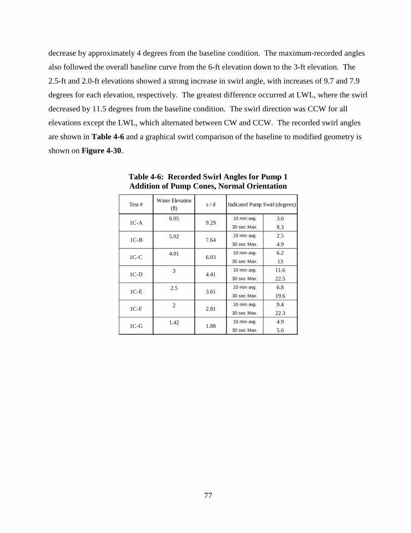
77
decrease by approximately 4 degrees from the baseline condition. The maximum-recorded angles
also followed the overall baseline curve from the 6-ft elevation down to the 3-ft elevation. The
2.5-ft and 2.0-ft elevations showed a strong increase in swirl angle, with increases of 9.7 and 7.9
degrees for each elevation, respectively. The greatest difference occurred at LWL, where the swirl
decreased by 11.5 degrees from the baseline condition. The swirl direction was CCW for all
elevations except the LWL, which alternated between CW and CCW. The recorded swirl angles
are shown in Table 4-6 and a graphical swirl comparison of the baseline to modified geometry is
shown on Figure 4-30.
Table 4-6: Recorded Swirl Angles for Pump 1 Addition of Pump Cones, Normal Orientation
6.05 10 min avg. 3.630 sec Max. 8.3
5.02 10 min avg. 2.530 sec Max. 4.9
4.01 10 min avg. 6.230 sec Max. 13
3 10 min avg. 11.630 sec Max. 22.5
2.5 10 min avg. 6.830 sec Max. 19.6
2 10 min avg. 9.430 sec Max. 22.3
1.42 10 min avg. 4.930 sec Max. 5.6
Test #Water Elevation
(ft) Indicated Pump Swirl (degrees)s / d
1C-F
1C-G
1C-A
1C-B
1C-C
1C-D
1C-E
9.29
7.64
6.03
4.41
3.61
2.81
1.88

78
Figure 4-30: Pump 1 swirl angles, normal orientation, baseline geometry
with and without pump cones (flow = 250 gpm/pump)
The pump #2 tests showed excellent correlation in average swirl angle from the 6-ft elevation to
the 2.5-ft elevation, with a maximum differential of 0.7 degrees recorded. Similar to pump 1, the
major difference occurred at LWL elevation, with a recorded decrease of 7.0 degrees from the
baseline geometry. The maximum recorded swirl angle also showed a good correlation to the
baseline data from the 6-ft to the 3-ft elevations. An increase of 4.6 degrees and 7.6 degrees was
recorded at the 2.5-ft and 2-ft elevations, respectively. The largest differential was at the LWL,
with a recorded decrease of 19.3 degrees in swirl angle. The swirl direction was CCW at
elevations 6 ft and 5 ft, both CCW and CW at 4 ft and CW at 3 ft down to 2 ft. The LWL
experienced both CW and CCW rotation. The recorded swirl angles are shown in Table 4-7 and a
graphical swirl comparison of the baseline to modified geometry is shown on Figure 4-31.
0
1
2
3
4
5
6
0 5 10 15 20 25 30
Elev
atio
n (f
eet)
Swirl Angle (degrees))
10-min Avg
30-sec Max
LWL
10-min Avg with Cones
30-sec Max with Cones

79
Table 4-7: Recorded Swirl Angles for Pump 2 Addition of Pump Cones, Normal Orientation
Figure 4-31: Pump 2 swirl angles, normal orientation, baseline geometry
with and without pump cones (flow = 250 gpm/pump)
6.03 10 min avg. 2.830 sec Max. 4.2
5 10 min avg. 2.730 sec Max. 5.1
4.01 10 min avg. 3.230 sec Max. 6.7
3 10 min avg. 7.530 sec Max. 15.8
2.51 10 min avg. 14.730 sec Max. 30.9
2 10 min avg. 17.430 sec Max. 29.2
1.42 10 min avg. 4.930 sec Max. 9.4
2C-D
2C-E
2C-A
2C-B
2C-C
Indicated Pump Swirl (degrees)
9.26
7.61
6.03
4.41
2C-F
2C-G
s / d
3.63
2.81
1.88
Test # Water Elevation (ft)
0
1
2
3
4
5
6
0 5 10 15 20 25 30 35
Wat
er E
leva
tion
(ft)
Swirl Angle (degrees)
10-min Avg
30-sec Max
LWL
10-min Avg with Cones
30-sec Max with Cones
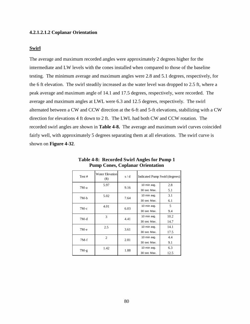
80
4.2.1.2.1.2 Coplanar Orientation
Swirl
The average and maximum recorded angles were approximately 2 degrees higher for the
intermediate and LW levels with the cones installed when compared to those of the baseline
testing. The minimum average and maximum angles were 2.8 and 5.1 degrees, respectively, for
the 6 ft elevation. The swirl steadily increased as the water level was dropped to 2.5 ft, where a
peak average and maximum angle of 14.1 and 17.5 degrees, respectively, were recorded. The
average and maximum angles at LWL were 6.3 and 12.5 degrees, respectively. The swirl
alternated between a CW and CCW direction at the 6-ft and 5-ft elevations, stabilizing with a CW
direction for elevations 4 ft down to 2 ft. The LWL had both CW and CCW rotation. The
recorded swirl angles are shown in Table 4-8. The average and maximum swirl curves coincided
fairly well, with approximately 5 degrees separating them at all elevations. The swirl curve is
shown on Figure 4-32.
Table 4-8: Recorded Swirl Angles for Pump 1 Pump Cones, Coplanar Orientation
5.97 10 min avg. 2.830 sec Max. 5.1
5.02 10 min avg. 3.130 sec Max. 6.1
4.01 10 min avg. 530 sec Max. 9.4
3 10 min avg. 10.230 sec Max. 14.7
2.5 10 min avg. 14.130 sec Max. 17.5
2 10 min avg. 4.430 sec Max. 9.1
1.42 10 min avg. 6.330 sec Max. 12.5
1.88
7M-f
7M-g
7M-d
7M-e
7M-b
7M-c
7M-a
Test #Water Elevation
(ft) Indicated Pump Swirl (degrees)s / d
9.16
7.64
6.03
4.41
3.61
2.81
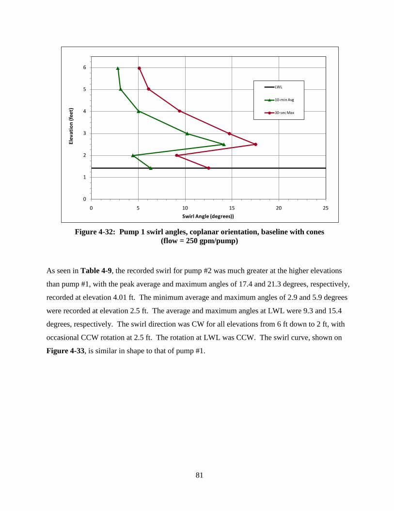
81
Figure 4-32: Pump 1 swirl angles, coplanar orientation, baseline with cones
(flow = 250 gpm/pump)
As seen in Table 4-9, the recorded swirl for pump #2 was much greater at the higher elevations
than pump #1, with the peak average and maximum angles of 17.4 and 21.3 degrees, respectively,
recorded at elevation 4.01 ft. The minimum average and maximum angles of 2.9 and 5.9 degrees
were recorded at elevation 2.5 ft. The average and maximum angles at LWL were 9.3 and 15.4
degrees, respectively. The swirl direction was CW for all elevations from 6 ft down to 2 ft, with
occasional CCW rotation at 2.5 ft. The rotation at LWL was CCW. The swirl curve, shown on
Figure 4-33, is similar in shape to that of pump #1.
0
1
2
3
4
5
6
0 5 10 15 20 25
Elev
atio
n (f
eet)
Swirl Angle (degrees))
LWL
10-min Avg
30-sec Max

82
Table 4-9: Recorded Swirl Angles for Pump 2 Pump Cones, Coplanar Orientation
Figure 4-33: Pump 2 swirl angles, coplanar orientation, baseline with cones
(flow = 250 gpm/pump)
6.01 10 min avg. 6.930 sec Max. 10.6
5.04 10 min avg. 11.130 sec Max. 18.5
4.01 10 min avg. 17.430 sec Max. 21.3
3.02 10 min avg. 1030 sec Max. 12.5
2.51 10 min avg. 2.930 sec Max. 5.9
2.01 10 min avg. 4.230 sec Max. 9.4
1.42 10 min avg. 9.330 sec Max. 15.4
1.88
2.838M-f
8M-g
Test #Water Elevation
(ft) Indicated Pump Swirl (degrees)
8M-a
8M-b
8M-c
8M-d
8M-e
s / d
7.67
6.03
4.44
3.63
9.23
0
1
2
3
4
5
6
0 5 10 15 20 25
Elev
atio
n (f
eet)
Swirl Angle (degrees))
LWL
10-min Avg
30-sec Max

83
4.2.1.2.1.3 Testing Summary
The normal orientation was unacceptable in terms of free-surface and subsurface vortices for the
baseline condition, with free-surface vortices present at selected conditions and subsurface air-
cores documented at all water levels below 3.5 ft (s/d < 5.2). The pump swirl was typically
deemed acceptable for the high-water operating conditions above 3.5 ft, but found to be
unacceptable at water levels below 3.5 ft for all conditions. The installation of pump cones (to
suppress the subsurface vortices) had a marginal effect on pump swirl for elevations down to 3 ft
for both pumps. An increase in swirl was seen at elevations 2.5 ft and 2 ft for both pumps and a
decrease was recorded at LWL for both pumps, with a significant decrease (+ 10 degrees) in the
maximum angle.
There were no free-surface vortices present for the coplanar orientation, as the surface energy was
sufficiently high to prevent formation. Subsurface air-core vortices were documented under both
pumps for all LWL tests (s/d = 1.88), with the exception of the single pump 1 test. However
vortices were present at the higher IWL condition. The swirl was found to be unacceptable at
pump 1 for all conditions and pump 2 for all conditions except the 2-pump LWL. The pump
cones increased the swirl angles 3-5 degrees at both pumps at the IWL and LWL.
4.2.1.2.2 Addition of 45-Degree Fillet
4.2.1.2.2.1 Normal Orientation
A 45-degree fillet was installed in the wet well to assess the design under solid-bearing liquid
operation. The pump cones were retained to prevent the formation of subsurface vortices.
Flow patterns
The flow patterns for the 1-pump tests at the LWL were similar to the predicted CFD results for
the 2-pump operation. Although the flow was skewed towards the operating pump, the rotation
around each pump was in a single direction throughout the depth of the wet well. The flow around
pump #1 was in a CCW direction, and pump #2 a CW direction, as indicated by the swirlmeter
and dye. There was a fairly high level of surface turbulence due to the reduced wet well volume.

84
The flow patterns in the wet well changed with increased water elevation, as indicated by the
change in swirl direction at elevations above 2.5 ft for each pump.
Vortices
Free-surface:
There were no unacceptable free-surface vortices (Type 3 or above) present for any of the tests
conducted for pumps either #1 or 2.
Swirl
The maximum and average recorded swirl angles, shown in Table 4-10, were much closer in
value with the addition of the fillet. The maximum angles were approximately 50% greater than
the averages, as opposed to 100%-200% for the no-fillet conditions. The lowest swirl angles for
pump #1 were once again recorded at the 5-ft elevation, with an average and maximum angle of
4.5 degrees and 6.8 degrees, respectively. The highest swirl angles were recorded at the LWL,
with average and maximum angles of 177 and 22.4 degrees, respectively. The overall shape of the
curve, shown on Figure 4-34, is similar to the baseline condition, with lower angles at the 5-ft and
2.5-ft elevations, giving the curve a sideways “W” shape. The swirl direction was CW for
elevations 6 ft down to 3 ft. A change in direction to CCW occurred prior to the 2.5-ft elevation
and remained CCW for the remaining water levels down to LWL. Although more consistent than
the baseline conditions, the swirl angles are still deemed unacceptable in accordance with the HI
criteria.

85
Table 4-10: Recorded Swirl Angles for Pump 1 45-Degree Fillet & Pump Cones, Normal Orientation
Figure 4-34: Pump 1 swirl angles, normal orientation, modified geometry
(flow = 250 gpm/pump)
s / d
6.03 10 min avg. 5.830 sec Max. 8.5
5.1 10 min avg. 4.530 sec Max. 6.8
4 10 min avg. 9.630 sec Max. 13.1
2.99 10 min avg. 5.430 sec Max. 10.1
2.49 10 min avg. 5.330 sec Max. 8
2.01 10 min avg. 14.430 sec Max. 18.3
1.42 10 min avg. 17.730 sec Max. 22.4
16D
16E
16F
16G 1.88
16C
7.77
6.01
4.39
3.59
2.83
Test #Water Elevation
(ft)
16A
Indicated Pump Swirl (degrees)
9.26
16B
0
1
2
3
4
5
6
0 5 10 15 20 25 30
Wat
er E
leva
tion
(ft)
Swirl Angle (degrees)
10-min Avg
30-sec Max
LWL

86
As seen in Table 4-11, the swirl angles recorded at pump #2 were very different from the baseline
conditions, in that, where the baseline geometry had low angles at the higher elevations, the fillet
geometry produced relatively high angles for all elevations of 3 ft and above. The highest average
angle of 15.2 degrees was recorded at the 4-ft elevation and the maximum angle of 20.8 degrees
was recorded at LWL. There was a dramatic decrease in swirl angle at the 2.5-ft elevation, with
an average and maximum angle of 2.5 and 4.4 degrees, respectively. The swirl direction was
CCW for all elevations between 6 ft and 3 ft. Transitional flow was present at elevation 2.5 ft, as
both CW and CCW rotations were recorded. The rotation was CW for the 2 ft and LWLs. The
curve representing the swirl angles is shown on Figure 4-35. All swirl angles with the exception
of those recorded at the 2.5-ft elevation are deemed unacceptable in accordance with the HI
criteria.
Table 4-11: Recorded Swirl Angles for Pump 2 45-Degree Fillet & Pump Cones, Normal Orientation
s / d
6.03 10 min avg. 11.430 sec Max. 14.5
5 10 min avg. 9.830 sec Max. 12.7
4.04 10 min avg. 15.230 sec Max. 17.1
3 10 min avg. 12.630 sec Max. 17.1
2.48 10 min avg. 2.530 sec Max. 4.4
2.01 10 min avg. 10.430 sec Max. 18.6
1.42 10 min avg. 14.930 sec Max. 20.8
7.61
6.07
4.41
3.58
2.83
1.88
17F
17G
Test #Water Elevation
(ft)
17A
17B
17C
17D
17E
Indicated Pump Swirl (degrees)
9.26

87
Figure 4-35: Pump 2 swirl angles, normal orientation, modified geometry
(flow = 250 gpm/pump)
4.2.1.2.2.2 Coplanar Orientation
Flow Patterns
The model was tested for the two 1-pump operating conditions, as the 2-pump condition was
deemed unnecessary. The flow patterns within the wet well were similar for both conditions, with
higher surface velocities along the backside of the pumps, resulting in general CW rotation of the
surface flow. The reduction of the wet well volume due to the fillet translated to an increase in the
% blockage caused by the pumps and stands, forcing the water over the top of the stands. Flow
deflected around the lead pump was drawn downward on the open side of the wet well and flowed
around the fillet at lower depths. This resulted in the flow under the pump bells to rotate in a
CCW direction for both pumps, as indicated by the swirl meters.
0
1
2
3
4
5
6
0 5 10 15 20 25 30
Wat
er E
leva
tion
(ft)
Swirl Angle (degrees)
10-Min Avg
30-sec Max
LWL

88
Vortices
Free-surface:
There were no free-surface vortices observed for any test conducted.
Swirl
Pump #1 produced the most favorable swirl results of all the conditions tested. As seen in Table
4-12, the average swirl angle ranged from 2.3 degrees to 6.4 degrees for elevations ranging from
5.78 ft down to 1.95 ft. The maximum angle for the same conditions ranged from 4.3 degrees to
9.7 degrees, with the highest swirl in the range occurring at elevation 2.52 ft. The highest swirl
angles were recorded once the water elevation dropped to the crown of the pipe, with average and
maximum ranges of 7.4 to 14.2 degrees and 13.3 to 27.3 degrees, respectively. The highest swirl
was recorded at LWL. The swirl direction was CW from elevation 6 ft to 4 ft, as well as 2.5 ft.
Both CW and CCW rotations were recorded at 3 ft, 2 ft and LWL. The swirl angle curves are seen
on Figure 4-36.

89
Table 4-12: Recorded Swirl Angles for Pump 1 45-Degree Fillet & Pump Cones, Coplanar Orientation
s / d
1.42 10 min avg. 14.230 sec Max. 27.3
1.56 10 min avg. 10.430 sec Max. 16.7
1.67 10 min avg. 7.430 sec Max. 13.3
1.78 10 min avg. 13.230 sec Max. 18.3
1.95 10 min avg. 3.530 sec Max. 5.4
2.02 10 min avg. 2.930 sec Max. 4.8
2.28 10 min avg. 3.730 sec Max. 7.6
2.52 10 min avg. 4.930 sec Max. 9.7
2.81 10 min avg. 2.330 sec Max. 4.5
3.05 10 min avg. 2.930 sec Max. 4.7
3.62 10 min avg. 2.630 sec Max. 4.3
4.06 10 min avg. 3.130 sec Max. 4.9
5.02 10 min avg. 6.430 sec Max. 8.0
5.78 10 min avg. 6.030 sec Max. 7.5
22I
22C
22M
22L
22K
22J
22H
22G
22F
22E
22D
2.46
22B
22A
19
Test #Water Elevation
(ft)Indicated Pump Swirl
(degrees)
1.88
2.11
2.28
2.73
2.84
3.26
3.64
4.11
4.49
5.40
6.11
7.64
8.86

90
Figure 4-36: Pump 1 swirl angles, coplanar orientation, modified geometry
(flow = 250 gpm/pump)
The recorded swirl for pump #2 was unlike that of pump #1. The highest average swirl was
experienced at water elevations between 5.79 and 4.01 ft, with documented angles ranging from
11.1 to 15.2 degrees, respectively. The lowest angles of 5.1 and 3.6 degrees were recorded at
elevations 3.06 and 2.03 ft, respectively. An angle of 11 degrees was recorded at LWL. The
maximum angles ranged from 5.7 degrees at elevation 2.03 ft, to 18.4 degrees at elevation 4.01 ft.
The swirl direction was CCW at elevations of 6 ft down to 4 ft. Both CW and CCW rotations
were recorded at all elevations below 4 ft. The swirl recorded swirl data is presented in Table 4-
13 and the corresponding curve is shown on Figure 4-37.
The swirl data for pumps #1 and 2 appear to be more unsteady at the low elevations than
previously tested conditions. However, this may be due to the additional data points collected at
elevations below 2 ft for these tests.
0
1
2
3
4
5
6
0 5 10 15 20 25 30
Wat
er E
leva
tion
(ft)
Swirl Angle (degrees)
10-Min Avg
30-sec Max
LWL

91
Table 4-13: Recorded Swirl Angles for Pump 2 45-Degree Fillet & Pump Cones, Coplanar Orientation
s / d
1.42 10 min avg. 1130 sec Max. 16.6
1.56 10 min avg. 8.530 sec Max. 13.5
1.68 10 min avg. 10.230 sec Max. 16.9
1.81 10 min avg. 6.230 sec Max. 11.3
1.93 10 min avg. 9.430 sec Max. 17.2
2.03 10 min avg. 3.630 sec Max. 5.7
2.28 10 min avg. 5.330 sec Max. 8.5
2.54 10 min avg. 830 sec Max. 13.7
2.79 10 min avg. 830 sec Max. 16.3
3.06 10 min avg. 5.130 sec Max. 11.8
4.01 10 min avg. 15.230 sec Max. 18.4
4.84 10 min avg. 12.830 sec Max. 15.8
5.79 10 min avg. 11.130 sec Max. 13.3
Indicated Pump Swirl (degrees)
23C
Test #
23B
Water Elevation (ft)
20
23A
1.88
2.11
2.30
2.51
23H
23I
23F
23G
23L
23K
23J
23D
23E
4.51
6.03
7.35
8.87
2.70
2.86
3.26
3.67
4.07

92
Figure 4-37: Pump 2 swirl angles, coplanar orientation, modified geometry
(flow = 250 gpm/pump)
4.2.1.2.2.3 Addition of a Flow Diverter
In an attempt to break up the inflow jet that exists with the normal orientation, a 3.5” diameter
column was installed along the centerline of the inlet at a position two-thirds the distance up the
slope, as shown on Figure 4-38. The column diverted the flow towards the center of each pump,
thereby reducing the overall rotation of the flow within the wet well. Various smaller pipe sizes
and locations were tested prior to the final selection. The pipe diameter was limited in size to
reduce the likelihood of rags getting impinged on the upstream face.
Vortices
The resulting flow pattern within the wet well allowed for Type 3 dye-core vortices to form on the
upstream side of each pump at elevation 2.5 ft and at elevation 2.25 ft for pump 2. The vortices
occurred for more than 10% of the time.
0
1
2
3
4
5
6
0 5 10 15 20 25 30
Wat
er E
leva
tion
(ft)
Swirl Angle (degrees)
10-min Avg
30-sec Max
LWL

93
Figure 4-38: Influent flow diverter modification

94
Swirl
The addition of the flow diverter dramatically improved the swirl entering each pump. As seen in
Table 4-14, the pump #1 average and maximum recorded swirl for water levels from 6.01 down to
2.26 ft ranged from 1.1 to 3.7 degrees, and 1.7 to 8.1 degrees, respectively. Although the HI only
allows a maximum angle of 5 degrees (up to 7), the swirl went above 5 degrees only 5% of the
time at the 2.51 and 2.26 water elevations. As with many of the tests conducted, the highest
average and maximum angles of 12.1 and 18.6 degrees, respectively, occurred at LWL. The swirl
direction was both CW and CCW for elevations 6 ft down to 3 ft. Steady CCW rotations were
recorded from elevation 2.25 ft to LWL. A graphical comparison of the swirl angle with and
without the diverter is shown on Figure 4-39.
Table 4-14: Recorded Swirl Angles for Pump 1 45-Degree Fillet, Pump Cones & Flow Diverter
Normal Orientation
s / d
1.42 10 min avg. 12.130 sec Max. 18.6
2 10 min avg. 9.530 sec Max. 11
2.26 10 min avg. 3.730 sec Max. 8.1
2.51 10 min avg. 2.330 sec Max. 5.2
3 10 min avg. 1.630 sec Max. 2.2
4.03 10 min avg. 1.930 sec Max. 2.8
5 10 min avg. 1.230 sec Max. 2.3
6.01 10 min avg. 1.130 sec Max. 1.7
6.01 10 min avg. 1.330 sec Max. 2.2
Test #Water Elevation
(ft)
16Me
16Ma
16M
16Mg
16Mf
16Mb
16Mc
16Mg
1.88
2.81
3.23
3.63
4.41
16Md
Indicated Pump Swirl (degrees)
6.06
7.61
9.23
9.23
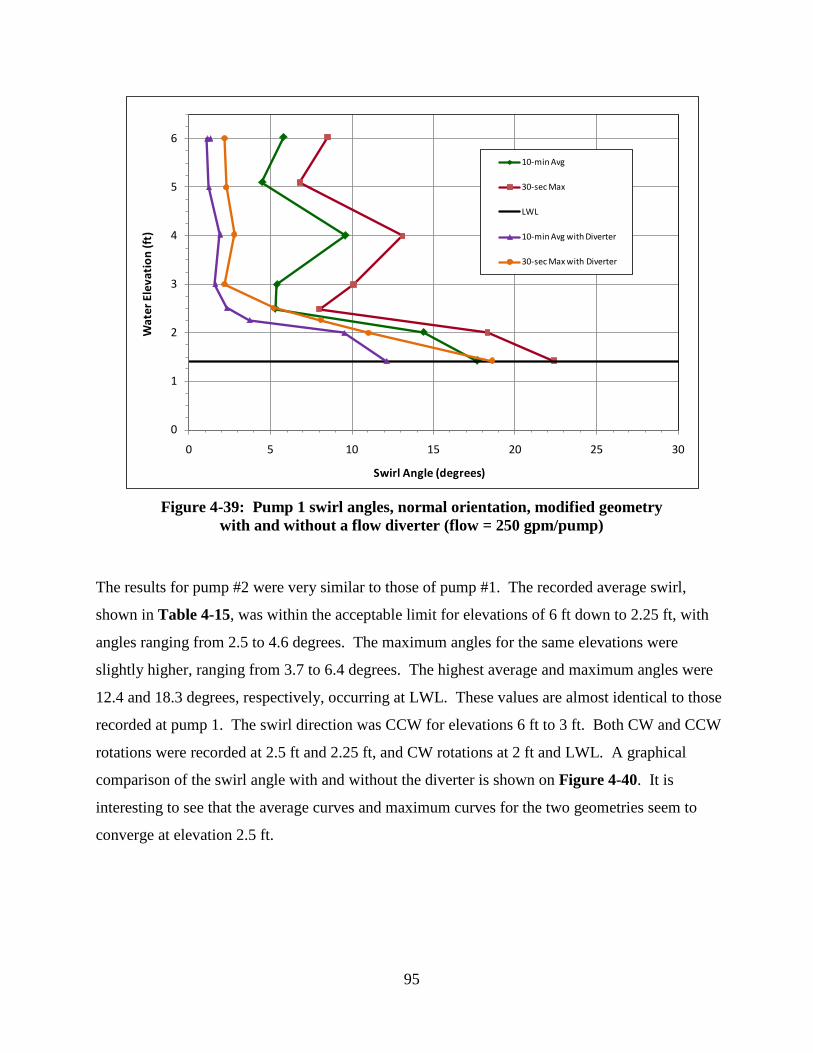
95
Figure 4-39: Pump 1 swirl angles, normal orientation, modified geometry
with and without a flow diverter (flow = 250 gpm/pump)
The results for pump #2 were very similar to those of pump #1. The recorded average swirl,
shown in Table 4-15, was within the acceptable limit for elevations of 6 ft down to 2.25 ft, with
angles ranging from 2.5 to 4.6 degrees. The maximum angles for the same elevations were
slightly higher, ranging from 3.7 to 6.4 degrees. The highest average and maximum angles were
12.4 and 18.3 degrees, respectively, occurring at LWL. These values are almost identical to those
recorded at pump 1. The swirl direction was CCW for elevations 6 ft to 3 ft. Both CW and CCW
rotations were recorded at 2.5 ft and 2.25 ft, and CW rotations at 2 ft and LWL. A graphical
comparison of the swirl angle with and without the diverter is shown on Figure 4-40. It is
interesting to see that the average curves and maximum curves for the two geometries seem to
converge at elevation 2.5 ft.
0
1
2
3
4
5
6
0 5 10 15 20 25 30
Wat
er E
leva
tion
(ft)
Swirl Angle (degrees)
10-min Avg
30-sec Max
LWL
10-min Avg with Diverter
30-sec Max with Diverter

96
Table 4-15: Recorded Swirl Angles for Pump 2 45-Degree Fillet, Pump Cones & Flow Diverter
Normal Orientation
Figure 4-40: Pump 2 swirl angles, normal orientation, modified geometry
with and without a flow diverter (flow = 250 gpm/pump)
s / d
1.42 10 min avg. 12.430 sec Max. 18.3
2.02 10 min avg. 9.730 sec Max. 12.6
2.25 10 min avg. 2.830 sec Max. 5.1
2.5 10 min avg. 2.530 sec Max. 4.8
3 10 min avg. 3.130 sec Max. 4.3
4.02 10 min avg. 4.630 sec Max. 6.4
5.04 10 min avg. 3.930 sec Max. 5.2
6 10 min avg. 2.730 sec Max. 3.7
9.21
Water Elevation (ft)
17M
17Md
17Me
17M
17Mg
17Mc
17Mb
17Ma
Test #Indicated Pump Swirl
(degrees)
1.88
2.84
3.21
3.61
4.41
6.04
7.67
0
1
2
3
4
5
6
0 5 10 15 20 25 30
Wat
er E
leva
tion
(ft)
Swirl Angle (degrees)
10-Min Avg
30-sec Max
LWL
10-Min Avg with Diverter
30-Sec Max with Diverter

97
4.2.1.2.2.4 Testing Summary
There were no free-surface or subsurface vortices documented for any tests conducted for the
normal or coplanar orientations. The reduced wet well volume due to the installation of the fillet
resulted in higher surface energy for all open channel influent flow conditions.
The recorded swirl angles at pump 1 for the normal orientation were unacceptable for all water
elevations tested. The overall swirl was lower than the baseline condition for most of the
operating conditions, with the exception of the LWL. Pump 2 showed unacceptable swirl at all
water elevations except 2.5 ft. The swirl angles were higher than the baseline condition at
elevations above 3 ft (s/d = 4.4) and at LWL (s/d = 1.88).
Pump 1 with the coplanar orientation showed an overall decrease in pump swirl from the baseline
condition, with the exception of the HWL and LWL. Acceptable swirl was recorded at most
conditions between 5 ft and 1.95 ft (s/d from 7.6 to 2.7). Pump 2 showed unacceptable swirl for
all water levels except 2 ft. The overall swirl was similar to that of the baseline condition with the
exception of increases between elevations 2 ft and 3 ft.
The installation of a flow diverter column in front of the inlet pipe reduced the pump swirl to
within acceptable limits at all elevations down to 2.5 ft for pump 1 (s/d = 3.6) and 2.25 ft for
pump 2 (s/d = 3.2).
The general flow patterns for the baseline 2-pump operating conditions agreed well with the CFD
results. However, when comparing the CFD velocity magnitudes under the pump bells for the
normal and coplanar orientations, it was anticipated that the coplanar design, with higher
rotational velocities, would produce higher pump swirl, which it did not. This may be due to a
higher level of turbulence under the bells, which the CFD results do not show. The modified
design was not physically tested under a 2-pump condition. However, the overall patterns within
the wet well were very similar to those predicted by the CFD simulations. The higher swirl angles
at pump 1 followed the predicted rotational velocities of the CFD. However, the recorded swirl
angles were higher for the coplanar design, which showed lower rotational velocities with the
CFD.

98
4.2.2 Dynamic Testing
As previously discussed in chapter 3, the swirl was evaluated under dynamic operating conditions,
with no inflow and 25 gpm and 125 gpm and an outflow of 250 gpm per pump. The “no-inflow”
testing was conducted with the influent pipe open, as well as blocked with an inflatable bladder
(selected conditions). This was done to assess the impact of the influent pipe draining on pump
swirl. If an open pipe proved to be unfavorable, the recommendation of adding a gate structure at
the inlet could be made. As cleanout of the wet wells are typically performed at low flow
conditions, the 25-gpm flow is of special interest in full drawdown operation and therefore, is
represented in red for clarity. All operating conditions were conducted with the pump cones
installed, as it was determined that they are required for eliminating the subsurface vortices.
Selected test conditions were also tested without pump cones.
All tests were conducted down to an elevation that caused sufficient air entrainment to break pump
siphon. The swirl direction is displayed on the graphs as either positive or negative values, with
positive representing CCW rotation and negative, CW rotation. The LWL is represented on each
graph with a solid black line.
Dynamic Swirl Repeatability
The dynamic swirl repeatability was conducted on various operating conditions throughout the
testing program. Since the swirl plots are based on swirl intensity and not elevations, the Standard
Deviation of the measurements are difficult to quantify. However, it can be seen qualitatively that
the swirl repeats very well under the dynamic test conditions, with maximum deviations of +/- 3
degrees. Repeatability graphs are shown on Figures 4-56 and 4-63.
4.2.2.1 Baseline testing
4.2.2.1.1 Normal Orientation
Pump 1
All dynamic tests conducted with the pump cones installed are shown in the compilation graph on
Figure 4-41. The swirl direction for all operating conditions was CCW. The 0-gpm condition
was the most stable, producing no swirl down to an elevation of approximately 1.5 ft. The

99
intensity and unsteadiness of the pump swirl increased sequentially with flow, with the 125-gpm
flow regularly producing angles from about 2 degrees to +10 degrees. The swirl was increasingly
higher and unsteady as the water level dropped below the LWL for all conditions. The maximum
recorded angles were approximately 24, 40 and 47 degrees for the 0, 25 and 125-gpm conditions,
respectively.
The 0-gpm flow test, shown on Figure 4-42, was conducted with the inlet pipe open and blocked.
Although the swirl was steadily increasing with lower water elevation, the swirl angles for the
blocked-pipe were below 5 degrees until approximately 0.75 ft and the maximum angle of about
9.5 degrees was recorded at a low elevation 0.5 ft.
As seen on Figure 4-43, the 25-gpm test experienced an initial swirl angle of about 8 degrees at
the 6-ft elevation, with a gradual decrease to 0 degrees at about 2.8 ft, followed by increasing swirl
down to shut-off.
The 125-gpm test was conducted with and without pump cones installed. As seen on Figure 4-44,
the pump swirl, on average, was slightly better without the cones. However, the swirl was
unsteady for both conditions and the difference in performance was not appreciable.
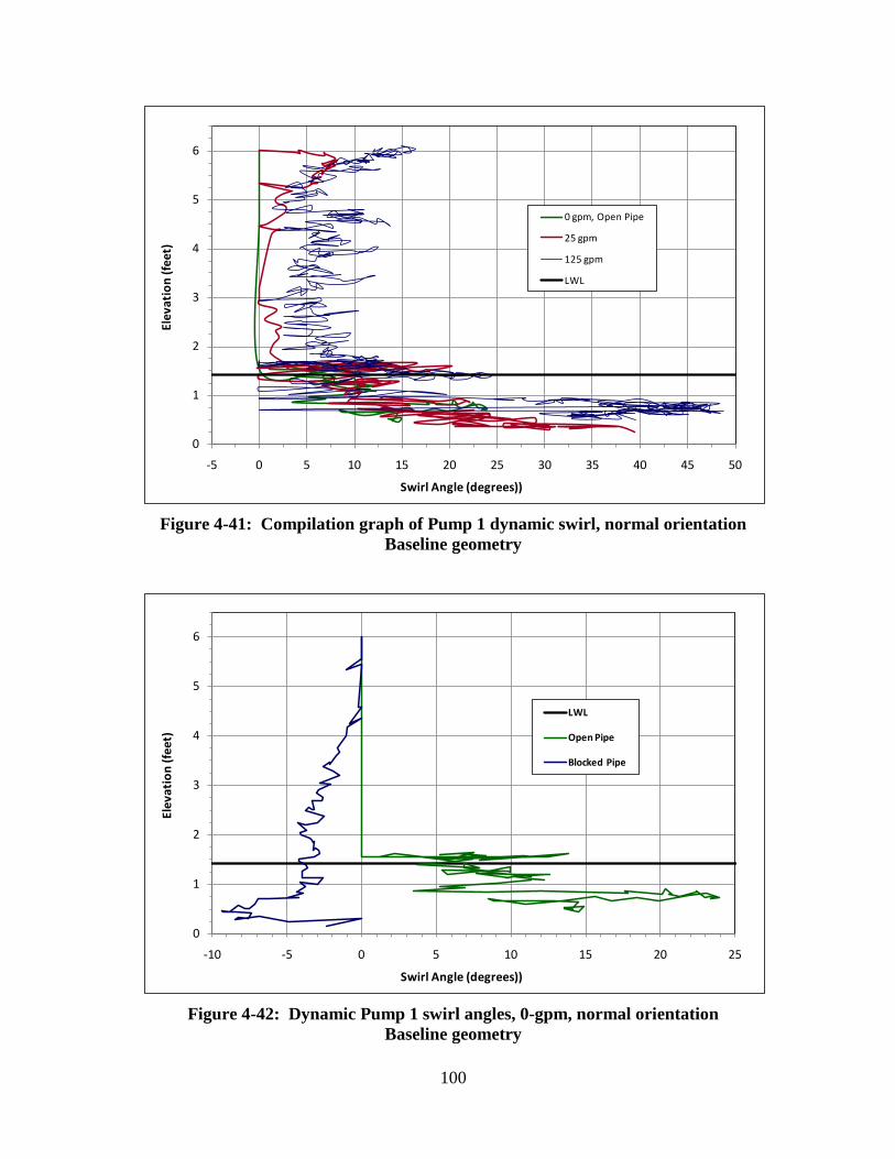
100
Figure 4-41: Compilation graph of Pump 1 dynamic swirl, normal orientation
Baseline geometry
Figure 4-42: Dynamic Pump 1 swirl angles, 0-gpm, normal orientation
Baseline geometry
0
1
2
3
4
5
6
-5 0 5 10 15 20 25 30 35 40 45 50
Elev
atio
n (f
eet)
Swirl Angle (degrees))
0 gpm, Open Pipe
25 gpm
125 gpm
LWL
0
1
2
3
4
5
6
-10 -5 0 5 10 15 20 25
Elev
atio
n (f
eet)
Swirl Angle (degrees))
LWL
Open Pipe
Blocked Pipe

101
Figure 4-43: Dynamic Pump 1 swirl angles, 25-gpm, normal orientation
Baseline geometry
Figure 4-44: Dynamic Pump 1 swirl angles, 125-gpm, normal orientation
Baseline geometry
0
1
2
3
4
5
6
-5 0 5 10 15 20 25 30 35 40
Elev
atio
n (f
eet)
Swirl Angle (degrees))
0
1
2
3
4
5
6
-20 -15 -10 -5 0 5 10 15 20 25 30 35 40 45 50
Elev
atio
n (f
eet)
Swirl Angle (degrees))
Without Cones
LWL
With Cones
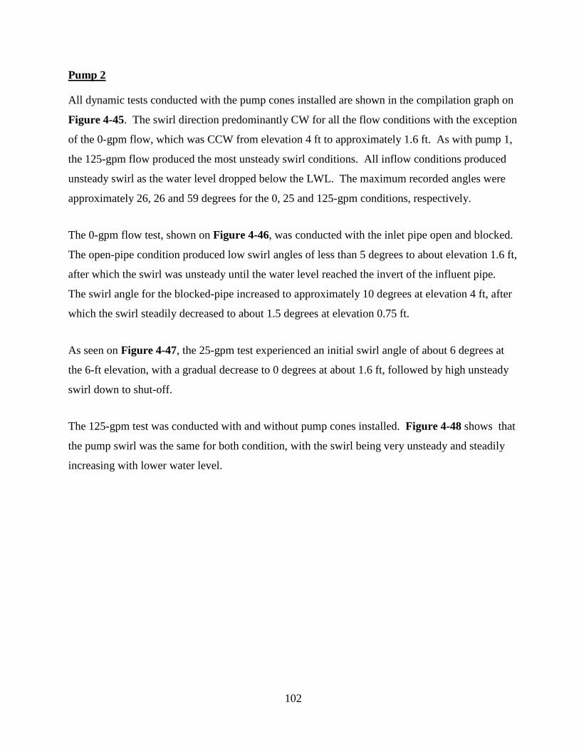
102
Pump 2
All dynamic tests conducted with the pump cones installed are shown in the compilation graph on
Figure 4-45. The swirl direction predominantly CW for all the flow conditions with the exception
of the 0-gpm flow, which was CCW from elevation 4 ft to approximately 1.6 ft. As with pump 1,
the 125-gpm flow produced the most unsteady swirl conditions. All inflow conditions produced
unsteady swirl as the water level dropped below the LWL. The maximum recorded angles were
approximately 26, 26 and 59 degrees for the 0, 25 and 125-gpm conditions, respectively.
The 0-gpm flow test, shown on Figure 4-46, was conducted with the inlet pipe open and blocked.
The open-pipe condition produced low swirl angles of less than 5 degrees to about elevation 1.6 ft,
after which the swirl was unsteady until the water level reached the invert of the influent pipe.
The swirl angle for the blocked-pipe increased to approximately 10 degrees at elevation 4 ft, after
which the swirl steadily decreased to about 1.5 degrees at elevation 0.75 ft.
As seen on Figure 4-47, the 25-gpm test experienced an initial swirl angle of about 6 degrees at
the 6-ft elevation, with a gradual decrease to 0 degrees at about 1.6 ft, followed by high unsteady
swirl down to shut-off.
The 125-gpm test was conducted with and without pump cones installed. Figure 4-48 shows that
the pump swirl was the same for both condition, with the swirl being very unsteady and steadily
increasing with lower water level.

103
Figure 4-45: Compilation graph of Pump 2 dynamic swirl, normal orientation
Baseline geometry
Figure 4-46: Dynamic Pump 2 swirl angles, 0-gpm, normal orientation
Baseline geometry
0
1
2
3
4
5
6
-60 -55 -50 -45 -40 -35 -30 -25 -20 -15 -10 -5 0 5 10
Wat
er E
leva
tion
(ft)
Swirl Angle (degrees)
25 gpm
125 gpm
LWL
0 gpm
0
1
2
3
4
5
6
-30 -25 -20 -15 -10 -5 0 5 10
Wat
er E
leva
tion
(ft)
Swirl Angle (degrees)
Blocked Pipe
LWL
Open Pipe
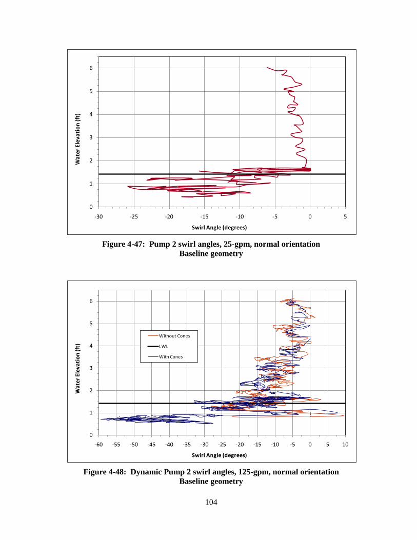
104
Figure 4-47: Pump 2 swirl angles, 25-gpm, normal orientation
Baseline geometry
Figure 4-48: Dynamic Pump 2 swirl angles, 125-gpm, normal orientation
Baseline geometry
0
1
2
3
4
5
6
-30 -25 -20 -15 -10 -5 0 5
Wat
er E
leva
tion
(ft)
Swirl Angle (degrees)
0
1
2
3
4
5
6
-60 -55 -50 -45 -40 -35 -30 -25 -20 -15 -10 -5 0 5 10
Wat
er E
leva
tion
(ft)
Swirl Angle (degrees)
Without Cones
LWL
With Cones

105
4.2.2.1.2 Coplanar Orientation
Pump 1
All dynamic tests conducted with the pump cones installed are shown in the compilation graph on
Figure 4-49. The swirl direction was CW for all inflow conditions from initiation of testing down
to just above the LWL, after which the direction changed to CCW (125-gpm), or switched
between CCW and CW, as in the 0 and 25-gpm flows. The 125-gpm flow produced the most
unsteady swirl conditions. All inflow conditions produced unsteady swirl as the water level
dropped below the LWL. The maximum recorded angles were approximately 13, 11 and 22
degrees for the 0, 25 and 125-gpm conditions, respectively. This is considerably better than the
pump-1 normal orientation swirl. Each test is shown on separate figures for clarity.
The 0-gpm flow test, shown on Figure 4-50, was conducted with the inlet pipe open. The swirl
steadily increased with lowering water elevation, with a maximum angle of less than 5 degrees
down to about 1.5 ft. A change in swirl direction is seen between elevations 1.5 ft and 1.1 ft. A
blocked-pipe test was not conducted on this pump.
As seen on Figure 4-51, the 25-gpm test had swirl angles of less than 3 degrees for all water
levels down to about the 1.6-ft elevation, after which the swirl was unsteady.
Figure 4-52 shows that the pump swirl for the 125-gpm test is beyond the acceptable limit of 5
degrees for a considerable amount of the time. The swirl was very unsteady throughout the test
and experienced an abrupt direction change at an elevation of about 1.7 ft.

106
Figure 4-49: Compilation graph of Pump 1 dynamic swirl, coplanar orientation
Baseline geometry
Figure 4-50: Dynamic Pump 1 swirl angles, 0-gpm, coplanar orientation
Baseline geometry
0
1
2
3
4
5
6
-15 -10 -5 0 5 10 15 20 25
Elev
atio
n (f
eet)
Swirl Angle (degrees))
0 gpm
25 gpm
125 gpm
LWL
0
1
2
3
4
5
6
-15 -10 -5 0 5 10
Elev
atio
n (f
eet)
Swirl Angle (degrees))

107
Figure 4-51: Dynamic Pump 1 swirl angles, 25-gpm, coplanar orientation
Baseline geometry
Figure 4-52: Dynamic Pump 1 swirl angles, 125-gpm, coplanar orientation
Baseline geometry
0
1
2
3
4
5
6
-15 -10 -5 0 5 10 15
Elev
atio
n (f
eet)
Swirl Angle (degrees))
0
1
2
3
4
5
6
-15 -10 -5 0 5 10 15 20 25
Elev
atio
n (f
eet)
Swirl Angle (degrees))
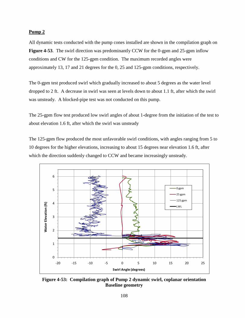
108
Pump 2
All dynamic tests conducted with the pump cones installed are shown in the compilation graph on
Figure 4-53. The swirl direction was predominantly CCW for the 0-gpm and 25-gpm inflow
conditions and CW for the 125-gpm condition. The maximum recorded angles were
approximately 13, 17 and 21 degrees for the 0, 25 and 125-gpm conditions, respectively.
The 0-gpm test produced swirl which gradually increased to about 5 degrees as the water level
dropped to 2 ft. A decrease in swirl was seen at levels down to about 1.1 ft, after which the swirl
was unsteady. A blocked-pipe test was not conducted on this pump.
The 25-gpm flow test produced low swirl angles of about 1-degree from the initiation of the test to
about elevation 1.6 ft, after which the swirl was unsteady
The 125-gpm flow produced the most unfavorable swirl conditions, with angles ranging from 5 to
10 degrees for the higher elevations, increasing to about 15 degrees near elevation 1.6 ft, after
which the direction suddenly changed to CCW and became increasingly unsteady.
Figure 4-53: Compilation graph of Pump 2 dynamic swirl, coplanar orientation
Baseline geometry
0
1
2
3
4
5
6
-20 -15 -10 -5 0 5 10 15 20 25
Wat
er E
leva
tion
(ft)
Swirl Angle (degrees)
0 gpm
25 gpm
125 gpm
LWL
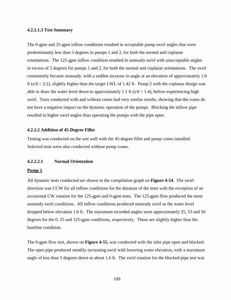
109
4.2.2.1.3 Test Summary
The 0-gpm and 25-gpm inflow conditions resulted in acceptable pump swirl angles that were
predominantly less than 5 degrees in pumps 1 and 2, for both the normal and coplanar
orientations. The 125-gpm inflow condition resulted in unsteady swirl with unacceptable angles
in excess of 5 degrees for pumps 1 and 2, for both the normal and coplanar orientations. The swirl
consistently became unsteady, with a sudden increase in angle at an elevation of approximately 1.6
ft (s/d = 2.2), slightly higher than the target LWL of 1.42 ft. Pump 2 with the coplanar design was
able to draw the water level down to approximately 1.1 ft (s/d = 1.4), before experiencing high
swirl. Tests conducted with and without cones had very similar results, showing that the cones do
not have a negative impact on the dynamic operation of the pumps. Blocking the inflow pipe
resulted in higher swirl angles than operating the pumps with the pipe open.
4.2.2.2 Addition of 45-Degree Fillet
Testing was conducted on the wet well with the 45-degree fillet and pump cones installed.
Selected tests were also conducted without pump cones.
4.2.2.2.1 Normal Orientation
Pump 1
All dynamic tests conducted are shown in the compilation graph on Figure 4-54. The swirl
direction was CCW for all inflow conditions for the duration of the tests with the exception of an
occasional CW rotation for the 125-gpm and 0-gpm tests. The 125-gpm flow produced the most
unsteady swirl conditions. All inflow conditions produced unsteady swirl as the water level
dropped below elevation 1.6 ft. The maximum recorded angles were approximately 25, 53 and 56
degrees for the 0, 25 and 125-gpm conditions, respectively. These are slightly higher than the
baseline condition.
The 0-gpm flow test, shown on Figure 4-55, was conducted with the inlet pipe open and blocked.
The open pipe produced steadily increasing swirl with lowering water elevation, with a maximum
angle of less than 5 degrees down to about 1.6 ft. The swirl rotation for the blocked-pipe test was

110
steady but unacceptable, with swirl angles of about 7 to 10 degrees recorded down below the 1–ft
elevation.
As seen on Figure 4-56, the 25-gpm test produced consistent swirl angles of 0 to 5 degrees for all
water levels down to about the 1.6-ft elevation, after which the swirl was unsteady. Three tests
were conducted which showed a high degree of testing repeatability. A comparison plot with and
without pump cones is shown on Figure 4-57. As previously noted, the cones had little effect on
pump swirl.
Figure 4-58 shows the pump swirl for the 125-gpm inflow with and without pump cones. On
average, both conditions produced acceptable swirl below 5 degrees. The swirl was slightly better
with the cones than without, but the difference is not appreciable. Occasional spikes of about 6
degrees are seen in both test results. The swirl became very unsteady at an elevation of about 1.7
ft.
Figure 4-54: Compilation graph of Pump 1 dynamic swirl, normal orientation
Modified geometry
0
1
2
3
4
5
6
-5 0 5 10 15 20 25 30 35 40 45 50 55 60
Wat
er E
leva
tion
(ft)
Swirl Angle (degrees)
0 gpm
25 gpm
125 gpm
LWL

111
Figure 4-55: Dynamic Pump 1 swirl angles, 0-gpm, normal orientation
Modified geometry:
Figure 4-56: Dynamic Pump 1 swirl angles, 25-gpm, normal orientation
Modified geometry with repeat tests
0
1
2
3
4
5
6
-15 -10 -5 0 5 10 15 20 25 30 35 40 45
Wat
er E
leva
tion
(ft)
Swirl Angle (degrees)
Blocked Pipe
LWL
Open Pipe, No Cones
0
1
2
3
4
5
6
-5 0 5 10 15 20 25 30 35 40 45 50 55
Wat
er E
leva
tion
(ft)
Swirl Angle (degrees)

112
Figure 4-57: Dynamic Pump 1 swirl angles, 25-gpm, normal orientation
Modified geometry
Figure 4-58: Dynamic Pump 1 swirl angles, 125-gpm, normal orientation
Modified geometry
0
1
2
3
4
5
6
-15 -10 -5 0 5 10 15 20 25 30 35 40 45
Wat
er E
leva
tion
(ft)
Swirl Angle (degrees)
With Cones
LWL
Without Cones
0
1
2
3
4
5
6
-5 0 5 10 15 20 25 30 35 40 45 50 55 60
Wat
er E
leva
tion
(ft)
Swirl Angle (degrees)
With Cones
LWL
Without Cones
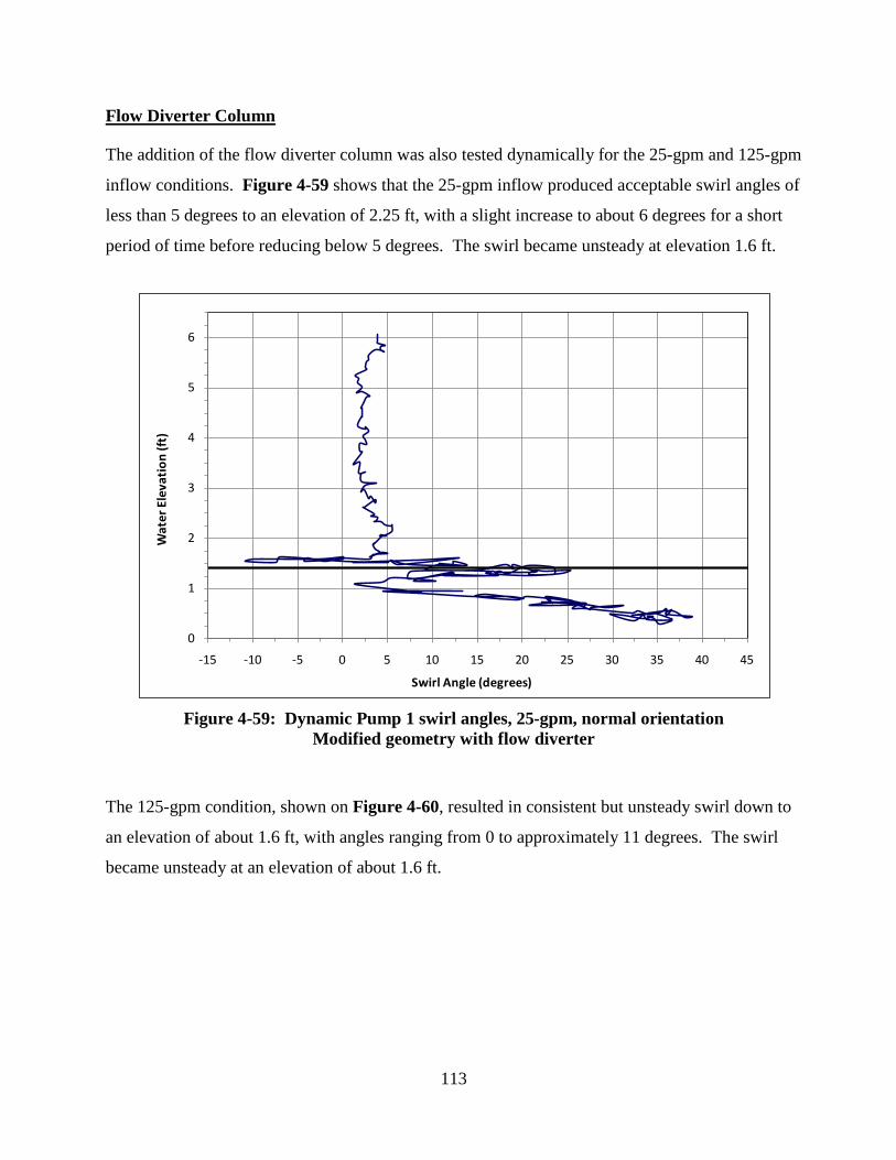
113
Flow Diverter Column
The addition of the flow diverter column was also tested dynamically for the 25-gpm and 125-gpm
inflow conditions. Figure 4-59 shows that the 25-gpm inflow produced acceptable swirl angles of
less than 5 degrees to an elevation of 2.25 ft, with a slight increase to about 6 degrees for a short
period of time before reducing below 5 degrees. The swirl became unsteady at elevation 1.6 ft.
Figure 4-59: Dynamic Pump 1 swirl angles, 25-gpm, normal orientation
Modified geometry with flow diverter
The 125-gpm condition, shown on Figure 4-60, resulted in consistent but unsteady swirl down to
an elevation of about 1.6 ft, with angles ranging from 0 to approximately 11 degrees. The swirl
became unsteady at an elevation of about 1.6 ft.
0
1
2
3
4
5
6
-15 -10 -5 0 5 10 15 20 25 30 35 40 45
Wat
er E
leva
tion
(ft)
Swirl Angle (degrees)
114
Figure 4-60: Dynamic Pump 1 swirl angles, 125-gpm, normal orientation
Modified geometry with flow diverter
Pump 2
All dynamic tests conducted are shown in the compilation graph on Figure 4-61. The swirl was
low for the 0-gpm and 25-gpm inflow conditions, with angles of less than 1-degree at 0-gpm and
approximately 3 degrees for the 25-gpm flow down to elevation 1.6 ft. The swirl direction was
both CW and CCW for the 25-gpm and 125-gpm flow conditions. The 125-gpm flow produced
the most unsteady swirl conditions. All inflow conditions produced unsteady swirl as the water
level dropped below elevation 1.6 ft. The maximum recorded angles were approximately 27, 52
and 80 degrees for the 0, 25 and 125-gpm conditions, respectively. These are substantially higher
than the baseline condition.
The 0-gpm flow test, shown on Figure 4-62, was conducted with the inlet pipe open and blocked.
The open pipe produced negligible swirl down to elevation 1.6 ft. The blocked-pipe test produced
increasing CCW swirl with dropping water level, peaking to about 9 degrees at elevation 1 ft. The
swirl direction transitioned to CW (0 degrees) at approximately 0.7 ft.
0
1
2
3
4
5
6
-20 -15 -10 -5 0 5 10 15 20 25 30 35 40 45 50 55 60 65
Wat
er E
leva
tion
(ft)
Swirl Angle (degrees)

115
As seen on Figure 4-63, the 25-gpm test produced consistent swirl angles of 0 to 3 degrees for all
water levels down to about the 1.7-ft elevation, after which the swirl was unsteady. Two tests
were conducted which showed good repeatability. The difference in swirl direction is due to the
fluctuation of the flow within the wet well and is expected at the low angles. A comparison plot
with and without pump cones is shown on Figure 4-64. The cones had little effect on pump swirl
down to approximately 0.8 ft. The pump swirl without the cones decreased below this elevation,
while the swirl with the cones increased. However, the operating time was to break siphon was
only about 9 seconds and therefore, the difference could be considered negligible
Figure 4-65 shows the pump swirl for the 125-gpm inflow with and without pump cones. The
swirl was unsteady for both conditions, with the direction changing direction throughout the tests.
The swirl was slightly better without the cones, but the difference is not appreciable. Occasional
spikes of about 6 degrees are seen in both test results. The swirl became very unsteady and was
virtually identical below an elevation of about 1.7 ft.
Figure 4-61: Compilation graph of Pump 2 dynamic swirl, normal orientation
Modified geometry
0
1
2
3
4
5
6
-50 -45 -40 -35 -30 -25 -20 -15 -10 -5 0 5 10 15
Wat
er E
leva
tion
(ft)
Swirl Angle (degrees)
0 gom
25 gpm
125 gpm
LWL

116
Figure 4-62: Dynamic Pump 2 swirl angles, 0-gpm, normal orientation
Modified geometry
Figure 4-63: Dynamic Pump 2 swirl angles, 25-gpm, normal orientation
Modified geometry
0
1
2
3
4
5
6
-40 -35 -30 -25 -20 -15 -10 -5 0 5 10 15
Wat
er E
leva
tion
(ft)
Swirl Angle (degrees)
Blocked Pipe
LWL
Open Pipe
0
1
2
3
4
5
6
-55 -50 -45 -40 -35 -30 -25 -20 -15 -10 -5 0 5 10
Wat
er E
leva
tion
(ft)
Swirl Angle (degrees)

117
Figure 4-64: Dynamic Pump 2 swirl angles, 25-gpm, normal orientation
Modified geometry
Figure 4-65: Dynamic Pump 1 swirl angles, 125-gpm, normal orientation
Modified geometry
0
1
2
3
4
5
6
-55 -50 -45 -40 -35 -30 -25 -20 -15 -10 -5 0 5 10
Wat
er E
leva
tion
(ft)
Swirl Angle (degrees)
With Cones
LWL
Without Cones
0
1
2
3
4
5
6
-90 -80 -70 -60 -50 -40 -30 -20 -10 0 10
Wat
er E
leva
tion
(ft)
Swirl Angle (degrees)
With Cones
LWL
Without Cones

118
Flow Diverter Column
The addition of the flow diverter column was also tested dynamically for the 25-gpm and 125-gpm
inflow conditions. Figure 4-66 shows that the 25-gpm inflow produced acceptable swirl angles of
less than 5 degrees to an elevation of approximately 1.6 ft, after which the swirl became unsteady.
Figure 4-66: Dynamic Pump 1 swirl angles, 25-gpm, normal orientation
Modified geometry with flow diverter
The 125-gpm condition, shown on Figure 4-67, resulted in swirl angles of about 5 degrees down
to an elevation of about 2.25 ft. The direction of swirl switched from CCW to CW at elevation 3
ft. Unacceptable swirl angles were recorded below elevation 2.3 ft.
0
1
2
3
4
5
6
-50 -45 -40 -35 -30 -25 -20 -15 -10 -5 0 5 10 15
Wat
er E
leva
tion
(ft)
Swirl Angle (degrees)

119
Figure 4-67: Dynamic Pump 1 swirl angles, 125-gpm, normal orientation
Modified geometry with flow diverter
4.2.2.2.2 Coplanar Orientation
Pump 1
25-gpm and 125-gpm inflow dynamic tests are shown in the compilation graph on Figure 4-68.
The swirl direction was CCW for the 25-gpm condition, from initiation of testing down to
elevation 1.6 ft, after which the direction switched between CCW and CW. The swirl angles were
very consistent, ranging between 3 degrees and 7 degrees for all water levels down to about the
1.6-ft elevation. The 125-gpm flow produced the most unsteady swirl conditions. The swirl
direction was predominantly CCW down to elevation 1.6 ft, with most of the swirl angles ranging
from 0 degrees to about 9 degrees. All inflow conditions produced unsteady swirl as the water
level dropped below elevation 1.6 ft. The maximum recorded angles were approximately 18 and
37 degrees for the 25 and 125-gpm conditions, respectively. These are slightly greater than the
baseline condition.
0
1
2
3
4
5
6
-50 -45 -40 -35 -30 -25 -20 -15 -10 -5 0 5 10
Wat
er E
leva
tion
(ft)
Swirl Angle (degrees)

120
Figure 4-68: Compilation graph of Pump 1 dynamic swirl, coplanar orientation
Modified geometry
Pump 2
25-gpm and 125-gpm inflow dynamic tests are shown in the compilation graph on Figure 4-69.
The swirl direction was CCW for the duration of both tests. The 25-gpm flow test produced low
swirl angles ranging from about 3 degrees to 5 degrees from the initiation of the test to about
elevation 1.7 ft, after which the swirl was unsteady. A few up to 7 degrees were recorded at the
higher water elevations. The 125-gpm flow produced the most unfavorable swirl conditions, with
angles ranging from 5 to 20 degrees for elevations down to about 1.6 ft. The maximum recorded
angles were approximately 23 and 36 degrees for the 25 and 125-gpm conditions, respectively.
These angles are higher than the baseline condition.
0
1
2
3
4
5
6
-15 -10 -5 0 5 10 15 20 25 30 35 40
Wat
er E
leva
tion
(ft)
Swirl Angle (degrees)
25 gpm
125 gpm
LWL

121
Figure 4-69: Compilation graph of Pump 2 dynamic swirl, coplanar orientation
Modified geometry
4.2.2.3 Testing Summary
The 0-gpm and 25-gpm inflow conditions resulted in acceptable pump swirl angles that were
predominantly less than 5 degrees in pumps 1 and 2 down to an elevation of 1.6, for both the
normal and coplanar orientations. The one exception was the 25-gpm pump 1 coplanar design,
which had angles up to about 7 degrees for almost 50% of the time. The 125-gpm inflow
condition resulted in unsteady swirl with unacceptable angles in excess of 5 degrees for pumps 1
and 2, for both the normal and coplanar orientations. However, the pump 1 and 2 normal and
pump 1 coplanar tests all produced results that may be considered acceptable if the criteria of 7
degrees is applied. The swirl consistently became unsteady, with a sudden increase in angle at an
elevation of approximately 1.6 ft (s/d = 2.2), slightly higher than the target LWL of 1.42 ft. Tests
conducted with and without cones had very similar results, showing that the cones do not have a
negative impact on the dynamic operation of the pumps. Blocking the inflow pipe resulted in
higher swirl angles than operating the pumps with the pipe open. The addition of the flow diverter
0
1
2
3
4
5
6
-5 0 5 10 15 20 25 30 35 40
Wat
er E
leva
tion
(ft)
Swirl Angle (degrees)
25 gpm
125 gpm
LWL

122
column did not show improved performance over the standard modified design with regards to
pump swirl. Multiple tests showed a high degree of test repeatability.
4.2.2.4 Cleanout Tests
To further assess the performance of the wet well in a solid-bearing liquid application, the
modified geometry (fillet and pump cones) was tested with the normal orientation to estimate the
removal rate of floatables and surface scum. Plastic pellets approximately 1/8” in diameter and
with a Specific Gravity (SG) of 0.90 were used to represent the surface scum. The model was
filled to the high water level (6 ft) and a measured volume of pellets was added to the surface.
The model was operated dynamically at inflows of 0-gpm and 25-gpm to represent typical
cleanout flow conditions.
Numerous tests were conducted on each pump for the 25-gpm inflow, to evaluate the effect of
varying the termination point from initial ingestion of air to full siphon break. The 0-gpm test was
terminated after the pump broke siphon. Any pellets remaining in the wet well after test
termination were collected and measured to determine the approximate removal efficiency.
Although the removal efficiencies were calculated based on measured quantities, the analysis is
more qualitative in nature, since the pellets do not possess the physical and cohesive properties of
actual surface scum.
Pump 1
The removal efficiency for the 25-gpm inflow ranged from 50% at the initiation of air ingestion, to
75% at a condition that represented siphon break (the siphon did not fully break in the model).
The removal efficiency for the 0-gpm inflow was 75% at siphon break. Test results are shown on
Table 4-16.
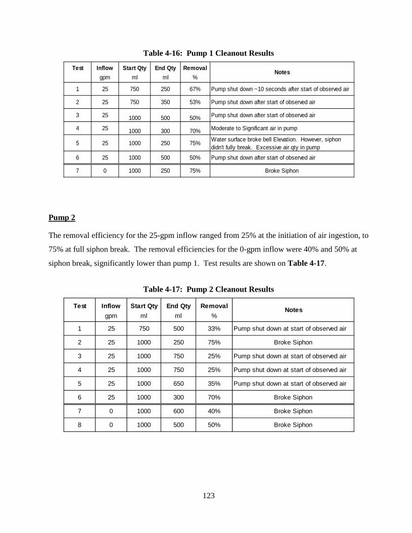
123
Table 4-16: Pump 1 Cleanout Results
Pump 2
The removal efficiency for the 25-gpm inflow ranged from 25% at the initiation of air ingestion, to
75% at full siphon break. The removal efficiencies for the 0-gpm inflow were 40% and 50% at
siphon break, significantly lower than pump 1. Test results are shown on Table 4-17.
Table 4-17: Pump 2 Cleanout Results
Test Inflow Start Qty End Qty Removalgpm ml ml %
1 25 750 250 67% Pump shut down ~10 seconds after start of observed air
2 25 750 350 53% Pump shut down after start of observed air
3 25 1000 500 50% Pump shut down after start of observed air
4 25 1000 300 70% Moderate to Significant air in pump
5 25 1000 250 75%
6 25 1000 500 50%
7 0 1000 250 75%
Water surface broke bell Elevation. However, siphon didn't fully break. Excessive air qty in pump
Pump shut down after start of observed air
Notes
Broke Siphon
Test Inflow Start Qty End Qty Removalgpm ml ml %
1 25 750 500 33% Pump shut down at start of observed air
2 25 1000 250 75%
3 25 1000 750 25% Pump shut down at start of observed air
4 25 1000 750 25% Pump shut down at start of observed air
5 25 1000 650 35%
6 25 1000 300 70%
7 0 1000 600 40%
8 0 1000 500 50%
Notes
Broke Siphon
Broke Siphon
Broke Siphon
Pump shut down at start of observed air
Broke Siphon

124
5.0 CHAPTER 5
CONCLUSIONS AND RECOMMENDATIONS
FOR FUTURE RESEARCH
A design evaluation was conducted on a Duplex Circular Wet Well using Computational Fluid
Dynamics (CFD) and Physical Modeling under various operating conditions and wet well
geometries. The CFD provided a comparative analysis of wet well flow patterns and the physical
model allowed for a detailed evaluation of pump performance.
5.1 CFD CONCLUSIONS
CFD simulations were conducted on a baseline and modified wet well geometry with 2 pumps
operating at a LWL of 1.35 ft. The pumps were tested in a normal (symmetrical) and coplanar
(inline) orientation to the influent pipe. The following conclusions are surmised:
• The results did not definitively show that either the normal or the coplanar design was advantageous for either the baseline or modified designs.
• Both pump orientations produced well-defined regions of rotation under the pump bells for both the baseline and modified design. Velocities of approximately 1.5 ft/s for the normal orientation and 2.5 ft/s for the coplanar orientation are predicted for the baseline condition. Velocities of approximately 3.5 ft/s for the normal orientation and 2.5 ft/s for the coplanar orientation are predicted for the modified geometry without pump cones.
• The coplanar orientation produced asymmetrical flow patterns for both the baseline and modified design due to the obstruction of the pump stands, which caused high surface velocities along the backside of the pumps.
• The baseline normal orientation produced symmetrical counter-rotating flows within the wet well, with the surface flow direction being opposite that of the flow under the pumps.

125
• The modified normal orientation produced symmetrical counter-rotating flows within the wet well, with constant flow direction throughout the wet well depth.
• The reduced wet well volume, due to the addition of the fillet in the modified design, resulted in higher velocities and surface energy for both designs. This will be beneficial for solids removal.
5.2 PHYSICAL MODEL CONCLUSIONS
A detailed evaluation of the pump performance in terms of vortex activity and pump suction swirl
was conducted on the physical model under steady state and dynamic operating conditions. Wet
well geometry included the baseline and modified designs and the pump were arranged in the
normal and coplanar orientations. The following conclusions are surmised:
• A coplanar orientation is not advantageous over a normal orientation as expected. Pump 2 consistently experienced higher pump swirl and both pumps 1 & 2 ingested impinged ir during free-discharge operating conditions.
• Dynamic operating conditions resulted in acceptable pump performance with regard to pump suction swirl under the no-inflow and 25-gpm inflow conditions.
• Steady state testing was very conservative when compared to dynamic testing and indicated unacceptable conditions at each pump for both wet well geometries and orientations.
• The installation of pump cones was required to eliminate air-core subsurface vortices which existed under both pumps, regardless of geometry or orientation.
• The addition of a flow diverter improved the conditions at the pumps for the modified geometry and normal orientation, as indicated by acceptable levels of recorded steady state pump swirl.
• The designated shut-off LWL needs to be raised to a minimum of 1.7 ft (s/d = 2.33) to reduce unstable pump flow which could lead to failure.
126
• Dynamic swirl angles increased with inflow under the baseline geometry at both pumps regardless of orientation. The inclusion of pump bell vanes to reduce swirl is recommended for clear-liquid applications.
• The pumps performed better with the influent pipe open than blocked for the no inflow condition.
• Wet well cleanout was better with 25-gpm of inflow when compared to no inflow.
5.3 RECOMMENDATIONS FOR FUTURE RESEARCH
The following recommendations are made for continued research of the DCWW:
• Testing of different side slope configurations may prove to be advantageous over the 45-degree fillet.
• The development of a floor-splitter design to reduce pump swirl that will not impinge solids will improve overall performance.
• Testing various influent pipe invert elevations to optimize the pipe invert-to-pump relationship will help optimize wet well design.
• Testing of various pump suction bells and associated sump designs.
• Testing a final selected design to assess solids removal.
REFERENCES
1. ASME, “Measurement of Fluid Flow in Pipes using Orifice, Nozzle and Venturi,”
American Society of Mechanical Engineers, MFC-3M-2004
2. ANSI/HI, “American National Standard for Pump Intake Design,” Hydraulic Institute,
ANSI, 9.8, 1998
3. Padmanabhan, M. and Hecker, G.E., "Scale Effects in Pump Sump Models," ASCE
Journal of Hydraulic Engineering, Vol. 110, No. 11, November, 1984.
3 Jain, A.K., Raju, K.G.R., and Garde, R.J., "Vortex Formation at Vertical Pump Intakes,"
ASCE Journal of Hydraulics Division, Vol. 104, 1978.
4 Anwar, H.O., Wellen, J.A., and Ampheltt, M.B., "Similarity of Free-Vortex at Horizontal
Intake," Journal of Hydraulic Research, IAHR, Vol. 16, No. 2, 1978.
5 Daggett, L. and Keulegan, G.H., "Similitude in Free-Surface Vortex Formations," Journal
of the Hydraulics Division, ASCE, November, 1974.
6 Jones, G.M., Sanks, R.L., Tchobanoglous, G., BossermanII, B.E., “Pump Station
Design,” Revised Third Edition, Butterworth-Heinemann, 2008

APPENDIX A
CFD MODEL PARAMETERS

APPENDIX A
DOUBLE precision version Title prep3d: version 9.3 win32-ifl 2008 hydr3d: version 9.3 win32-ifl 2008 version id: double mesh block 1 summary: x direction: # of real cells= 104 smallest cell = 5.0000E-02 largest cell = 5.0000E-02 maximum cell ratio = 1.0000E+00 (at cell # 104) y direction: # of real cells= 104 smallest cell = 5.0000E-02 largest cell = 5.0000E-02 maximum cell ratio = 1.0000E+00 (at cell # 105) z direction: # of real cells= 40 smallest cell = 5.0000E-02 largest cell = 5.0000E-02 maximum cell ratio = 1.0000E+00 (at cell # 15) mesh block 2 summary: x direction: # of real cells= 20 smallest cell = 5.0000E-02 largest cell = 5.0000E-02 maximum cell ratio = 1.0000E+00 (at cell # 15) y direction: # of real cells= 30 smallest cell = 5.0000E-02 largest cell = 5.0000E-02 maximum cell ratio = 1.0000E+00 (at cell # 30) z direction: # of real cells= 20 smallest cell = 5.0000E-02 largest cell = 5.0000E-02 maximum cell ratio = 1.0000E+00 (at cell # 17) mesh block 3 summary: x direction: # of real cells= 16 smallest cell = 2.5000E-02 largest cell = 2.5000E-02 maximum cell ratio = 1.0000E+00 (at cell # 16) y direction: # of real cells= 16 smallest cell = 2.5000E-02 largest cell = 2.5000E-02 maximum cell ratio = 1.0000E+00 (at cell # 17) z direction: # of real cells= 4 smallest cell = 2.5000E-02 largest cell = 2.5000E-02 maximum cell ratio = 1.0000E+00 (at cell # 5) mesh block 4 summary: x direction: # of real cells= 16 smallest cell = 2.5000E-02 largest cell = 2.5000E-02 maximum cell ratio = 1.0000E+00 (at cell # 16) y direction: # of real cells= 16 smallest cell = 2.5000E-02
APPENDIX A
largest cell = 2.5000E-02 maximum cell ratio = 1.0000E+00 (at cell # 17) z direction: # of real cells= 4 smallest cell = 2.5000E-02 largest cell = 2.5000E-02 maximum cell ratio = 1.0000E+00 (at cell # 5) ************************ total requested number of cells in all blocks: 446688 ************************ cad data min/max x coordinates = -4.187333E+00, 2.999880E+00 cad data min/max y coordinates = -4.187333E+00, 2.999880E+00 cad data min/max z coordinates = -4.999800E-01, 4.999800E+00 cad data min/max x coordinates = -9.999600E-01, -5.007906E-01 cad data min/max y coordinates = -2.497877E-01, 2.497869E-01 cad data min/max z coordinates = 4.266141E-01, 5.994574E-01 cad data min/max x coordinates = 4.999800E-01, 9.991493E-01 cad data min/max y coordinates = -2.497877E-01, 2.497869E-01 cad data min/max z coordinates = 4.266141E-01, 5.994574E-01 volume added to meet avrck ratio= 9.59551E-02 volume percentage added to meet avrck ratio= 0.267 % cell summary: total number of cells (active and passive) = 498752 total number of active cells = 316824 active cells include: real cells (used for solving flow equations) = 307446 open real cells = 299937 fully blocked real cells = 7509 standard boundary cells (used for boundary types 1 to 8) = 7834 inter-block boundary cells (store interpolated variables) = 1544 ************************************************** ** summary of mesh boundaries for mesh block 1 ** ************************************************** left boundary - solid wall right boundary - solid wall front boundary - inter-block open area = 5.43156E-01 back boundary - solid wall bottom boundary - solid wall top boundary - symmetry plane ************************************************** ** summary of mesh boundaries for mesh block 2 ** ************************************************** left boundary - solid wall

APPENDIX A
right boundary - solid wall front boundary - specified velocity initial flow rate = 1.12000E+00 flow vector: 0.000E+00 1.000E+00 0.000E+00 initial x-velocity = 0.00000E+00 initial z-velocity = 0.00000E+00 initial fluid height = 1.35000E+00 open area = 5.43083E-01 back boundary - inter-block open area = 5.43156E-01 bottom boundary - solid wall top boundary - solid wall ************************************************** ** summary of mesh boundaries for mesh block 3 ** ************************************************** left boundary - inter-block open area = 0.00000E+00 right boundary - inter-block open area = 0.00000E+00 front boundary - inter-block open area = 0.00000E+00 back boundary - inter-block open area = 0.00000E+00 bottom boundary - inter-block open area = 6.88301E-02 top boundary - inter-block open area = 0.00000E+00 ************************************************** ** summary of mesh boundaries for mesh block 4 ** ************************************************** left boundary - inter-block open area = 0.00000E+00 right boundary - inter-block open area = 0.00000E+00 front boundary - inter-block open area = 0.00000E+00 back boundary - inter-block open area = 0.00000E+00 bottom boundary - inter-block open area = 6.88302E-02 top boundary - inter-block open area = 0.00000E+00 open area mismatch at inter-block boundaries of all blocks as % of total open area at these mesh boundaries = 3.74784E-01 number of open regions in mesh is = 1 volume

APPENDIX A
1 3.59931E+01 estimated uncompressed flsgrf file size: 2 gb initial data print mesh volume summary: open volume = 3.59931E+01 component volume = 2.39131E+00 fluid volume at time zero = 2.45234E+01

APPENDIX B
MODEL DETAIL DRAWINGS

APPENDIX B
B-1: TANK DESIGN & MODIFICATIONS

APPENDIX B
B-2: ACRYLIC WINDOW DETAIL

APPENDIX B
B-3: ACRYLIC INFLUENT PIPE DETAIL

APPENDIX B
B-4: ALUMINIM FLOOR FRAME

APPENDIX B
B-5: VOLUTE MODIFICATION

APPENDIX B
B-6: ACRYLIC MODELED MOTOR DETAIL

APPENDIX B
B-7: SWIRL METER FLANGE

APPENDIX B
B-8: PUMP CONE DETAIL

APPENDIX B
B-9: FILLET TOE SUPPORT DETAIL

APPENDIX B
B-10: ACRYLIC FILLET SHEET LAYOUT
APPENDIX C
INSTRUMENTATION CALIBRATIONS

APPENDIX C
FLOW METER CALIBRATIONS
2-Inch Influent Meter

APPENDIX C
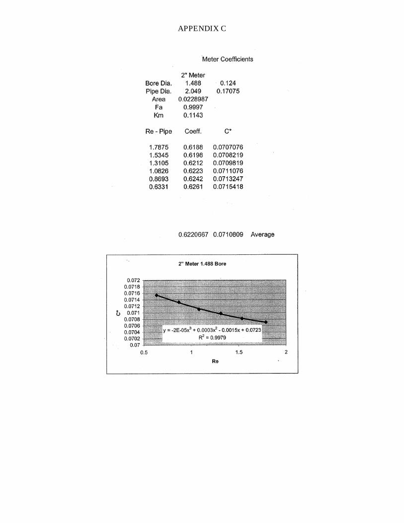
APPENDIX C

APPENDIX C

APPENDIX C
4-Inch Effluent Meters

APPENDIX C

APPENDIX C

APPENDIX C
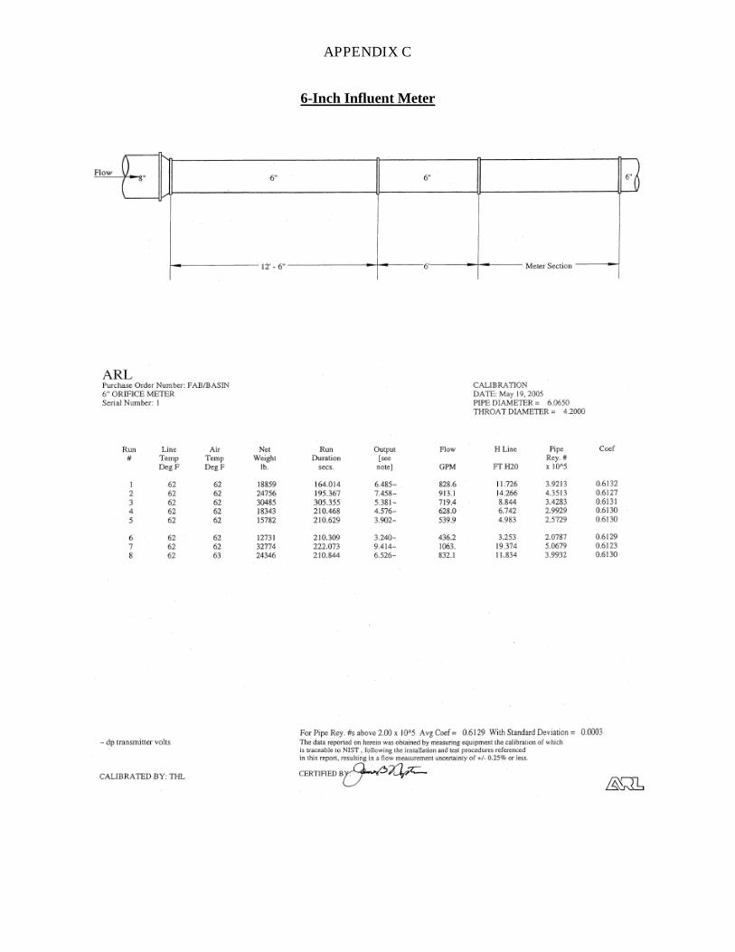
APPENDIX C
6-Inch Influent Meter

APPENDIX C
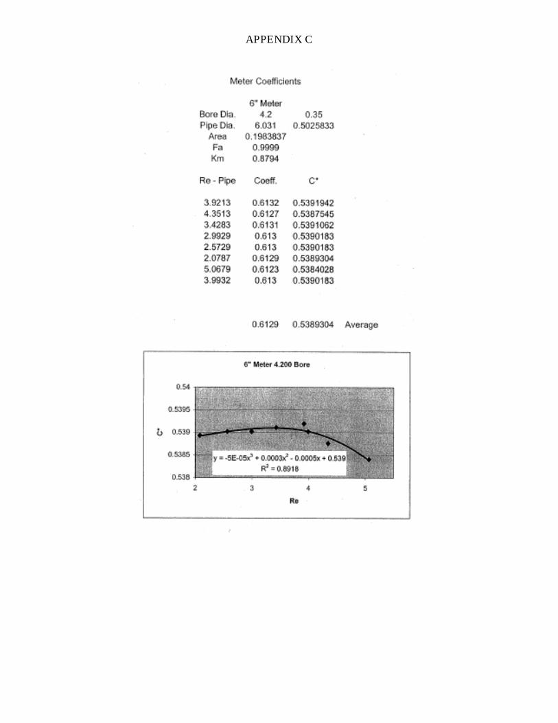
APPENDIX C

APPENDIX C

APPENDIX C
DIFFERENTIAL PRESSURE CELLS
Influent Flow Cell
Delta-H Delta-H Delta-H 0-72"inch ft psi Volts
0 0.000 0.000 2.0413.75 0.313 0.135 2.477.12 0.593 0.257 2.85916.68 1.390 0.602 3.9426.56 2.213 0.958 5.0837.53 3.128 1.354 6.33146.86 3.905 1.691 7.39857.02 4.752 2.057 8.55465.63 5.469 2.368 9.541
Channel #0 DP Cell - Influent
y = 0.3157x - 0.6444R² = 1
0.0
0.3
0.6
0.9
1.2
1.5
1.00 2.00 3.00 4.00 5.00 6.00 7.00 8.00
Del
ta-H
(psi
)
Volts
Channel #0 DP Cell - Influent

APPENDIX C
Effluent Flow Cell – Pump 1
Delta-H Delta-H Delta-H 0-240"inch ft psi Volts
0 0.000 0.000 1.9583.75 0.313 0.135 2.0797.12 0.593 0.257 2.1916.68 1.390 0.602 2.49626.56 2.213 0.958 2.82237.53 3.128 1.354 3.17846.86 3.905 1.691 3.48157.02 4.752 2.057 3.8165.63 5.469 2.368 4.09173.94 6.162 2.668 4.35883.13 6.9275 3.000 4.662
Channel 1 DP Cell #SWDP1 - Pump 1
y = 1.1106x - 2.1742R² = 1
0.0
0.5
1.0
1.5
2.0
2.5
3.0
1.00 2.00 3.00 4.00 5.00
Del
ta-H
(psi
)
Volts
Channel 1 DP Cell #SWDP1 - Pump 1

APPENDIX C
Effluent Flow Cell – Pump 2
Delta-H Delta-H Delta-H 0-240"inch ft psi Volts
0 0.000 0.000 1.9783.75 0.313 0.135 2.0987.12 0.593 0.257 2.20616.68 1.390 0.602 2.50726.56 2.213 0.958 2.82437.53 3.128 1.354 3.17546.86 3.905 1.691 3.47257.02 4.752 2.057 3.79465.63 5.469 2.368 4.06973.94 6.162 2.668 4.33183.13 6.9275 3.000 4.628
Channel 2 DP Cell #0617 - Pump 2
y = 1.1327x - 2.2406R² = 1
0.0
0.5
1.0
1.5
2.0
2.5
3.0
3.5
1.00 2.00 3.00 4.00 5.00
Del
ta-H
(psi
)
Volts
Channel 2 DP Cell #0617 - Pump 2

APPENDIX C
Water Elevation Cell
Delta-H Delta-H Delta-H 0-60"inch ft psi Volts
0 0.000 0.000 2.0433.75 0.313 0.135 2.2417.12 0.593 0.257 2.42616.68 1.390 0.602 2.92226.56 2.213 0.958 3.45237.53 3.128 1.354 4.03646.86 3.905 1.691 4.53357.02 4.752 2.057 5.06765.63 5.469 2.368 5.52373.94 6.162 2.668 5.95983.13 6.928 3.000 6.453
Channel 3 DP Cell #0622 - Water El.
y = 0.6799x - 1.389R² = 1
0.0
0.5
1.0
1.5
2.0
2.5
1.00 2.00 3.00 4.00 5.00 6.00 7.00
Del
ta-H
(psi
)
Volts
Channel 3 DP Cell #0622 - Water El.