-" I

t

DESIGN EQUATIONS OF SWEPT FREQUENCY SPECTRUM ANALYZERS FOR IN-FLIGHT VIBRATION ANALYSIS

i

https://ntrs.nasa.gov/search.jsp?R=19660025918 2018-06-29T06:44:07+00:00Z

TECH LIBRARY m H M

I llllll 11111 ill1 Ilil IIIII 11111 lllll Ill1 Ill1

DESIGN EQUATIONS O F SWEPT FREQUENCY SPECTRUM ANALYZERS

FOR IN-FLIGHT VIBRATION ANALYSIS

By Edward F. Mi l le r and David L. Wright

Lewis Resea rch Center Cleveland, Ohio

NATIONAL AERONAUTICS AND SPACE ADMINISTRATION

For sale by the Clearinghouse for Federal Scientific and Technical Information Springfield, Virginia 22151 - Price $2.00

The equations fo

FOR IN-FLIGHT VIBRATION ANALYSIS

by Edward F. Mil ler and David L. Wright

Lewis Research Center

SUMMARY

the design of swept frequency spectrum analyz

DESIGN EQUATIONS OF SWEPT FREQUENCY SPECTRUM ANALYZERS

rs a r e presented with the intended application being in-flight analysis of vibration data. is given to developing the optimum combination of the frequency-time function and the analyzing filter bandwidth. acceptable resolution and accuracy. discussed, and the frequency-time equation is developed for each-of these three types. The analyzer using a second-order sweep rate is shown to have the shortest sweep time, but it requires an expanding bandwidth filter and a decreasing averaging-time power de- tector. The linear sweep rate analyzer is shown to require less bandwidth per channel and is much less complex. The constant sweep rate analyzer is shown to have either very long sweep times o r poor frequency resolution; however, all three types of analyzers have bandwidth savings over real-time transmission of wide-band data.

Primary emphasis

The main criterion used is minimum sweep time coupled with Constant, linear, and second-order sweep rates are

I NT RO D UCTlON

A continuing problem in communication system design is transmitting many channels of wide-band data over a limited bandwidth transmission system. critical in transmission from a spacecraft or a launch vehicle, where increased band- width requires more weight and power, and consequently, reduced payload. The partic- ular problem that led to this investigation was the need to transmit from launch vehicles the results of a large number of vibration measurements.

Currently, NASA uses primarily the IRIG FM/FM (Inter-Range Instrumentation Group) standard telemetry format for the transmission of analog vibration signals from vehicles to the ground, and an extensive network of ground stations has been built to re- ceive data in this format. Often, the number of vibration measurements desired exceeds

The problem is most

b

the capacity of the IRIG FM/FM telemetry system. There are several ways to solve this problem. One method is to change the transmission system. Two transmission systems capable of transmitting many channels of real-time, wide-band data from space vehicles a r e DSB/FM (double-sideband/frequency modulation (ref. 1)) and SSB/FM (single- sideband/frequency modulation (ref. 2)). Another alternative is to use some form of data reduction before the data is transmitted. On-board data reduction reduces the transmis- sion bandwidth required and still allows the use of the IRIG FM/FM transmission system for the resulting low bandwidth channels. Spectrum analysis is the method of pretrans- mission data reduction that is considered in this report.

Spectrum analysis of a signal often gives sufficient information about the real-time signal. In many cases, the final form of vibration data is a plot of the power density of the signal as a function of frequency (or power spectral density). This form of the re- sult is important because it can show the frequencies present in the vibration source as well as the amplitudes and frequencies of the dominant vibration modes of the vehicle structure. However, the process of spectrum analysis is irreversible since no phase relations between the frequency components of a given signal a r e obtained; thus, spectrum analysis loses the actual time history of the vibration. In addition, relative phase meas- urements between two time functions cannot be made by comparing their spectrums. Even with these limitations spectrum analysis remains useful.

Theoretical work in spectrum analysis (refs. 3 and 4) was followed by the consider- ation of swept frequency spectrum analyzers with a constant sweep rate and a constant bandwidth filter (refs. 5 and 6). Commercially available airborne spectrum analyzers are of this type; however, they have the drawbacks of poor resolution and/or long sweep times. For random data, a spectrum analyzer with a linear sweep rate has better reso- lution and/or shorter sweep time than the constant sweep rate analyzer. rate analyzers have been used (to the authors' knowledge) only as ground equipment. A spectrum analyzer with a sweep rate proportional to frequency squared was mentioned by Bendat (ref. 7), but the frequency-time function was not derived.

In this report, the basic theoretical background for spectrum analysis is presented. The frequency-time functions a r e derived for the various types of swept frequency spec- trum analyzers. The development progresses from the simple case of a constant sweep rate analyzer operating on periodic signals through to the progressively more complex operations of constant, linear, and second-order sweep rate systems analyzing random signals. For each type of frequency sweep, the attainable performance, as given by the frequency-time function, is compared with the following desired specifications for air- borne spectrum analyzers (the list was compiled from discussions with those who use and reduce vibration data):

The linear sweep

2

Frequency range . . . . . . . . . . . . . . . . . . . . . . near zero to several kilohertz Allowable frequency e r ro r . . . . . . . . . . *lo percent of the frequency being analyzed Minimum resolvable bandwidth . . . . . . . *lo percent of the frequency being analyzed Allowable spectrum amplitude e r ror . . . . . . . . . . . . . . . . . . . . . *lo percent Sweep time . . . . . . . . . . . . . . . . . . . . . . . . . . . . . of the order of seconds

These desired specifications are shown to be incompatible and cannot be obtained in the analysis of random data. Even periodic data can only be analyzed with less than the desired accuracy in such a short sweep time.

In those cases where long sweep times o r reduced accuracies a r e tolerable, the in- flight spectrum analyzer may be used. The bandwidth savings resulting from the use of spectrum analyzers in these cases is discussed in the concluding section of this report.

A limitation of the swept frequency spectrum analyzers discussed in this report is that it is not practical to extend their lower frequency limit to "near zero, * * as listed in the desired specifications previously given. The frequency- time equations derived in this report show that low-frequency spectrum analyzers have extremely long sweep times and require very narrow filters to obtain good frequency resolution. spectrum analyzers have a practical low-frequency limit on the order of 100 hertz. low-frequency part of the signal is better handled by separate transmission of that portion of the time-varying signal followed by spectrum analysis on the ground.

The swept frequency The

BACKGROUND TO PROBLEM

Before proceeding to the details of the analysis, some necessary background infor- mation will be discussed.

Genera I B ac kg r ou n d

Characteristics of expected signals. - Since this report is concerned with the specific problem of transmitting vibration data, the assumed characteristics of such data will be discussed. source. frequency content of the resulting vibration. The mechanical Q, or sharpness of reso- nance, is assumed to be less than 10; thus, if the spectral peaks are to be resolved, analyzing filters with values of electrical Q much greater than 10 would be required. Moreover, the maximum mechanical Q is assumed to be independent of the resonant frequency. frequency increases.

First, the source causing the vibration is assumed to be a random noise The mechanical system coupled to this source acts as a filter that shapes the

Thus, the bandwidths of the resonances become progressively wider as the

3

In order to obtain meaningful data, the signal being analyzed must be stationary during the time of observation; that is, the probability distribution of the signal level must remain constant. The vibration signal will remain stationary as long as the source causing the vibration remains statistically invariant. Examples of events causing nonsta- tionarity would be turning on or turning off a rocket engine, changes in thrust, or changes in air turbulence surrounding the vehicle.

For the swept frequency spectrum analyzer, the minimum period of stationarity of the signal limits the total sweep time. When the signal is nonstationary, the spectrum changes with time. Thus, for the swept frequency spectrum analyzer the signal must be stationary for times on the order of the total sweep time. The minimum period of sta- tionarity can be somewhat less than the total sweep time since interpolation between suc- ceeding spectrums can give estimates of the spectrum between sweeps.

Types of spectrum analyzers. - There are two common types of analog spectrum analyzers. The simplest method of spectrum analysis is to measure the power from each filter in a group of band-pass filters whose center frequencies are spaced so that the filter pass bands cover the frequency range of the input signal. The power output of each filter is an approximation to the average power spectral density of the signal within the filter pass band. The swept frequency spectrum analyzer is the second common type of spec- trum analyzer and is the subject of this report. Its operation will be discussed in de- tail.

The analyzer shown in figure 1 is one of several ways of implementing the swept fre- quency analyzer. The frequency diagram is shown in figure 2. Basicaiiy, Ge a n a i m in figure 1 translates the signal spectrum to a higher frequency using suppressed carr ier amplitude modulation. At the high frequency, a single band-pass filter selects a narrow band of frequencies corresponding to a similar narrow band of frequencies of the input

band-pass Signal Mixer filter 9

Power spec- detector -trum

I 1 swept frequency oscillator

Figure 1. - Block diagram of typical swept frequency spectrum analyzer.

,-Analyzing ,-Signal / filter f l *A ,’ spectrum

0 fL fH fs fc Frequency

Figure 2 - Frequency d i i r a m of typical swept frequency spectrum analyzer. Lowest frequency to be ahalyzed fL; highest frequency to be analyzed fH; mixing frequency fs; center frequency f,.

spectrum. A sample of the power out- put of the filter is an approximation to the power spectral density within the corresponding signal frequency incre- ment. The filter is effectively swept through the signal spectrum by sweep- ing the mixing frequency fs. A disad- vantage of this analyzer is that both the filter and the power detector must have time to change their output values as they are swept through the spectrum. A major objective of this report is to show that the proper choice of the time dependence of the frequency sweep will

4

optimize the sweep time and the resolution for. the swept frequency spectrum analyzer. Before deriving the frequency-time equations for the constant, the linear, and the second- order sweep rate spectrum analyzers, some of the basic theory of spectrum analysis will be presented.

T h eo r et ica I B ac kg r o u n d

The basic restrictions on swept frequency spectrum analysis will be shown by first considering the spectrum analysis of periodic signals. Then the more complex case of analysis of random signals will be considered.

Spectrum analysis ~~~~ of periodic __ signals. - Periodic signals are representable by a Fourier series of harmonically related sinusoidal waves. The basis for such representa- tion is well known and will not be discussed here (see ref. 8 for a discussion of Fourier series).

constant with time. Such a spectrum may be resolved by a swept frequency spectrum analyzer with a sharp band-pass filter whose bandwidth is less than the minimum spacing between frequency components of the spectrum. Thus,

The spectrum for a periodic signal has discrete components whose amplitudes a r e

1 Bf < - TP

where

Bf effective filter bandwidth (bandwidth of the ideal rectangular filter that passes the same power as the real filter when both are excited by white noise)

period of the signal TP

Furthermore, the sweep rate of the analyzer must be slow enough to allow the filter response to come up to almost fu l l value before the analyzer moves on to another fre- quency. A band-pass filter excited by a sinusoidal signal a t its center frequency has an output response envelope with a time constant given by

1 Tc =- mBf

where Tc is the time constant of response.

5

I

Also, the output of the filter must be measured by a detector whose averaging time is long compared with the period of the filter output, which is a sine wave at the filter center frequency. Thus, the averaging time is given by

1 Td >> - fC

(3)

where

Td detector averaging time

fc filter center frequency

Using equations ( l ) , (2), and (3), one can design a spectrum analyzer for periodic signals. Spectrum analysis of random signals. - The measurement of the spectrum of a ran-

dom signal is not as straightforward. By its nature, a random signal has no periodicity, its value as a function of time cannot be precisely predicted, and, at best, only a prob- ability distribution for its values can be specified. Analyzing such functions requires some of the techniques of generalized harmonic analysis and probability theory. A brief introduction to the required techniques follows (for a thorough discussion see refs. 9 to 11. ).

The power spectral density (or mean square spectral density) of a stationary random function of time is defined as the Fourier transform of the autocorrelation function R(T). Let x(t) be the random function. Then

T lim 1 x(t) x(t+T)dt T - t m % /I R(T) =

and the power spectral density S(f) is given by

(Symbols a re defined in the appendix. ) The function S(f) has the property that

T Imm S(f)df = Mean square value of x(t) = t:m -$ x2(t)dt

(4)

Also,

6

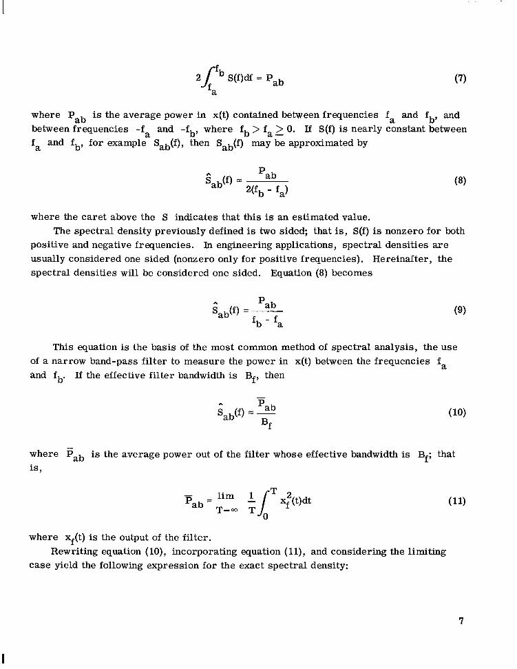
2 p S(f)df = Pab (7)

where Pab is the average power in x(t) contained between frequencies fa and fb, and between frequencies -fa and -fb, where fb > f > 0. Lf S(f) is nearly constant between fa and fb, for example sab(f), then Sab(f) may be approximated by

a -

where the caret above the S indicates that this is an estimated value.

positive and negative frequencies. usually considered one sided (nonzero only for positive frequencies). Hereinafter, the spectral densities will be considered one sided.

The spectral density previously defined is two sided; that is, S(f) is nonzero for both In engineering applications, spectral densities a re

Equation (8) becomes

L. 'ab s (f) = ___ ab f b - fa

(9)

This equation is the basis of the most common method of spectral analysis, the use of a narrow band-pass filter to measure the power in x(t) between the frequencies fa and fb' If the effective filter bandwidth is Bf, then

- where Pab is the average power out of the filter whose effective bandwidth is Bf; that is,

where xf(t) is the output of the filter.

case yield the following expression for the exact spectral density: Rewriting equation (lo), incorporating equation (ll), and considering the limiting

7

I

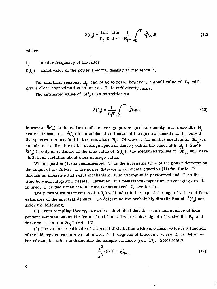
T S(fc) = lim lim 1 $(t)dt

Bf-0 T - L ~ BfT

where

center frequency of the filter

exact value of the power spectral density at frequency fc fC

S(fc)

For practical reasons, Bf cannot go to zero; however, a small value of Bf will

The estimated value of S(fc) can be written as give a close approximation as long as T is sufficiently large.

* T S(fc) = -!-/ xf2(t)dt

BfT 0

In words, $(fc) is the estimate of the average power spectra density in a andwidth Bf centered about fc. G(fc) is an unbiased estimator of the spectral density at fc only if the spectrum is constant in the bandwidth Bf. (However, for nonflat spectrums, 6(fc) is an unbiased estimator of the average spectral density within the bandwidth B . ) Since

*f &fc) is only an estimate of the true value of S(fc), the measured values of S(fc) will have statistical variation about their average value.

When equation (13) is implemented, T is the averaging time of the power detector on the output of the filter. If the power detector implements equation (11) for finite T through an integrate and reset mechanism, true averaging is performed and T is the time between integrator resets. However, if a resistance-capacitance averaging circuit is used, T is two times the RC time constant (ref. 7, section 4).

estimates of the spectral density. To determine the probability distribution of $(fc) con- sider the following:

(1) From sampling theory, it can be established that the maximum number of inde- pendent samples obtainable from a band-limited white noise signal of bandwidth Bf and duration T is n = 2BfT (ref. 12).

of the chi-square random variable with N-1 degrees of freedom, where N is the num- ber of samples taken to determine the sample variance (ref. 13). Specifically,

The probability distribution of &fc) will indicate the expected range of values of these

(2) The variance estimate of a normal distribution with zero mean value is a function

(14) 2 2

2 S

U

- (N- l ) = XN- 1

8

I

where

S sample variance

a true variance

XN- 1 chi-square random variable with N-1 degrees of freedom (the chi-square distri- bution is tabulated in statistical tables)

(3) For certain types of random functions, those which satisfy the quasi-ergodic hy- pothesis (ref. 11, ch. 7), the time average of the function equals the ensemble average; that is,

where p[x(t)] is the probability distribution of x(t). Equation (15) states that the mean square value of x(t) equals the second moment of x(t). The random functions considered will be assumed to satisfy the quasi- ergodic hypothesis.

(4) For a random variable x(t),

E[x 2 (t)] = Var x(t) -I- {E[x(t)]I2

(24-4 Second Variance Mean value moment of x(t) of x(t), quan- of x(t) tity squared

Applying equation (6) and steps (l), (2), (3), and (4) leads to the following conclusion: The power measured at the output of an ideal band-pass filter fed by white noise is an estimate of the variance of the band-limited white noise (because the noise has zero mean value), and thus the power is a function of chi-square with n- 1 or 2BfT- 1 degrees of freedom. The filter power is assumed to be measured using an averaging time T.

Therefore g(fc) is given by

The probability of &fc) being within a certain interval of S(fc) can be calculated as fol- lows:

9

I

Let

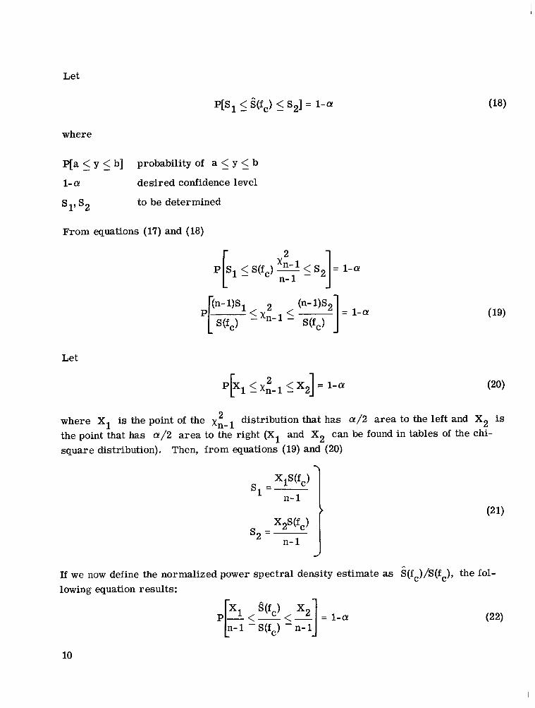
PIS1 < - $(fJ < - s2] = l-a!

where

P[a < - - y < b] probability of a < - - y < b

1- a! desired confidence level

to be determined S1’ s2

From equations (17) and (18)

Let

where X1 is the point of the x i - l distribution that has a / 2 area to the left and X2 is the point that has a!/2 area to the right (X1 and X2 can be found in tables of the chi- square distribution). Then, from equations (19) and (20)

If we now define the normalized power spectral density estimate as S(fc)/S(fc), the fol- lowing equation results:

10

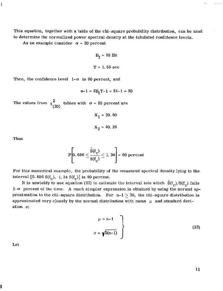
This equation, together with a table of the chi-square probability distribution, can be used to determine the normalized power spectral density at the tabulated confidence levels.

As an example consider a = 20 percent

Bf = 10 Hz

T = 1.55 sec

Then, the confidence level 1-a is 80 percent, and

n-1 = 2BfT-1 = 31-1 = 30

The values from x tables with a = 20 percent a r e (30)

X1 = 20.60

X2 = 40.26

Thus

P 0.686 < - I - For this numerical example, the probability of the measured spectral density lying in the interval [O. 686 S(fc), 1. 34 S(fc)] is 80 percent.

It is unwieldy to use equation (22) to estimate the interval into which i(fc)/S(fc) f a l l s 1-a percent of the time. A much simpler expression is obtained by using the normal ap- proximation to the chi-square distribution. For n-1 > 30, the chi-square distribution is approximated very closely by the normal distribution with mean ,u and standard devi- ation cr:

-

Let

11

I

where

w is the normal random variable, with mean p and standard deviation u.

One can find in normal probability tables the values of q that satisfy

P[-q <_ z 5 q] = 1-a!

where z is the standardized normal random variable ( p = 0 and o = 1). Now,

and equation (25) becomes

P[-q 5 w-I,L U < - q 1 = 1-a!

Using equations (23) and (24) in equation (26) results in

or

P

where the percent e r ror E is

J W,) S(fJ -

l - € < - < l + E - =1-a!

12

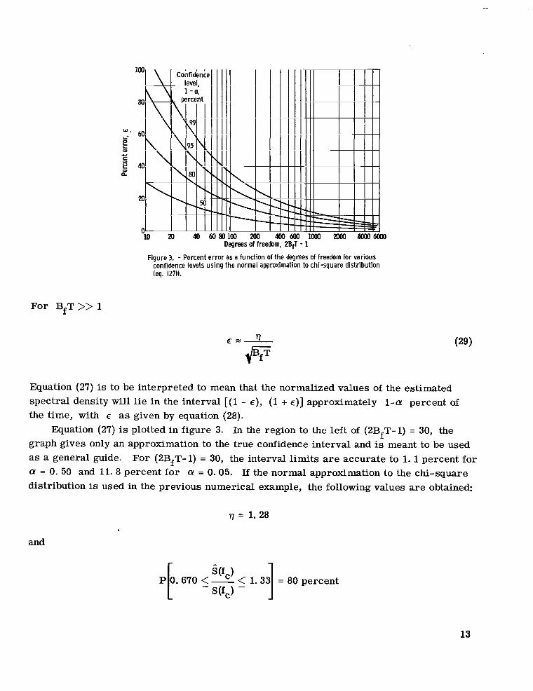
Figure 3. - Percent error as a function of the degrees of freedom for various confidence levels using the normal approximation to chi-square distribution (eq. (27)).

For BfT >> 1

Equation (27) is to be interpreted to mean that the normalized values of the estimated spectral density will lie in the interval [(l - E ) , (1 + E)] approximately 1-a! percent of the time, with E as given by equation (28).

Equation (27) is plotted in figure 3. graph gives only an approximation to the true confidence interval and is meant to be used as a general guide. a! = 0. 50 and 11. 8 percent for a! = 0.05. If the normal approximation to the chi-square distribution is used in the previous numerical example, the following values a re obtained:

In the region to the left of (2BfT-1) = 30, the

For (2BfT-1) = 30, the interval limits a r e accurate to 1.1 percent for

7 = 1.28

and

1.33 = 80 percent 1 13

which agrees with the limits obtained previously within about 2.3 percent.

on the estimated spectral density when a confidence level is given. BfT, equations (27) and (28) may be used.

analyzing filter did not enter into the analysis for random signals. the requirement that a number of independent samples of the power level be taken in each frequency interval. have had ample time to change from one level to another. Thus, taking 2BfT-1 independ- ent samples in each frequency interval guarantees that the filter response time has been exceeded many times.

analyzers will be discussed.

In summary, equation (22) is the exact expression used to obtain a confidence interval For large values of

The reader may recall equation (2) and might wonder why the response time of the The answer lies in

If the samples are to be truly independent, the filter output must

Now that sufficient background information has been introduced the design of spectrum

DESIGN

The theory of swept frequency spectrum analyzers will be applied first to the design for periodic signals. Then the theory will be applied to random signals, which are rep- resentative of flight vibration data.

Design for Periodic Signa ls

For periodic signals, there is no statistical uncertainty in the time function and equa- tions (l), (2), and (3) apply:

1 Bf <- TP

1 Tc = - “Bf

1 Td >> - fC

Equation (1) is satisfied by choosing a narrow band-pass filter as the analyzing filter. Equation (2) is satisfied by requiring each Fourier component to remain in the filter

14

long enough to allow the filter to come up to nearly f u l l response. Let the sweep rate of the analyzer be such that in time NITc the filter moves across a frequency span of width Bf (N is a numerical constant). If N1 = 3, the filter will be at approximately 95 percent 1 of its f u l l value as the Fourier component leaves the filter. For a constant sweep rate,

- = K1 dt

where

fi signal frequency being analyzed

- sweep rate dt

K1 sweep rate constant

Sweeping at a rate slow enough to allow adequate filter response and yet having minimum sweep time requires that

dt

Thus ,

2 Bf - mBf

K1=- -- NlTC N1

2 Bf - mBf

K1=- -- NlTC N1

Solving equation (30) subject to fi(0) = fL, where f L is the lowest frequency to be ana- lyzed, yields

fi(t) = Klt + f L (33)

The total sweep time ts may be found by using fi(ts) = fH, where fH is the highest fre- quency to be analyzed, in equation (33). Then solving for ts gives

15

Equations (32), (33), and (34) characterize the constant sweep rate spectrum analyzer for periodic signals.

The restrictions imposed by equation (3) have not yet been incorporated into the design equations. Assume that the filter center frequency fc in a swept frequency ana- lyzer with modulation is greater than 10 kilohertz. Then, from equation (3), the detector averaging time must be much greater than 100 microseconds. This criterion is easily met and in practical cases imposes no further restrictions on the sweep rate as given by equation (32).

straightforward. A filter bandwidth Bf is chosen to give what the user considers to be adequate resolution, with equation (1) used as a guide. The sweep rate is given by equa- tion (32), the frequency-time function to be implemented by a variable frequency oscil- lator is given by equation (33), and the total sweep time is given by equation (34).

2 2 total sweep time in equation (34) is inversely proportional to Bf . As a numerical ex-

ample consider the following:

The design of a constant sweep rate spectrum analyzer for periodic signals is

Notice in equation (32) that the sweep rate is directly proportional to Bf, while the

Bf = 10 HZ

fH = 2000 HZ

f L = 100 HZ

Choose

Then,

N1 = a

K1 = 100 Hz/sec

fi(t) = loot + 100

t = 19 sec S

16

This example has good resolution but a fairly long sweep time. If Bf were expanded to 20 hertz, the total sweep time would be only 4.8 seconds. The resolution would not have been degraded significantly; however, the system still would not meet the desired speci- fications listed in the INTRODUCTION because the minimum resolvable bandwidth would have been increased to 20 percent of the bandwidth center frequency at fL.

Note that this,analysis only applies to periodic data where there is no statistical un- certainty in the filter output. Spectrum analyzers for random data are discussed in the next section.

Design for Random Signals

Basic sweep rate equation. - Consider analyzing a spectral peak of width Bn with a filter of width Bf. First, to limit the amplitude error to E with a confidence level 1-a, the filter must be entirely within the peak Bn for a time T determined from

The use of this equation assumes that 2BfT-1 is sufficiently large that the normal ap- proximation to the chi-square distribution may be used.

yields approximately the same results as moving the filter through it in discrete steps (ref. 7). in a time T and still remain entirely within the peak for the duration T. Thus,

Secondly, it can be shown that continuously sweeping a filter through a spectrum

From these considerations the filter can only be swept Bn - Bf in frequency

dfi Afi Bn - Bf dt A t T

- - ---- (3 5)

This is the basic sweep rate equation. Optimization of the filter bandwidth. - For in-flight vibration data the mechanical Q

was assumed to be independent of the resonant frequency. Thus, if the minimum'resolv- able peak with center frequency fi is defined as Bn, then the following equation results from the universal resonance curve:

Bn=- 'i

Qmax

I

17

Clearly, if a filter of bandwidth Bf is to resolve a spectral peak of width Bn, then Bf must be less than Bn. Let

Bf = C Bn (37)

where C is a constant to be determined. For a fixed bandwidth filter

Bf=C(B,) =- f L

min Qmax

since the filter must be able to resolve a spectral peak at the frequency fL. Consider the optimum value for Bf or C. This means given E and q find Bf such that dfi/dt is a maximum; that is, solve for

Lo; 0 dBf dt

and

&(E!) < o dBf2 dt

Solving equation (28) for T and substituting in the basic sweep rate equation yield

dfi (Bn - Bf)2BfE 2 - - - -

2 2 27 + E dt

Now

2

= o

(39)

Thus,

18

Since

2

2 2 ““0 = - 46 < o

dt 2q + E dBf

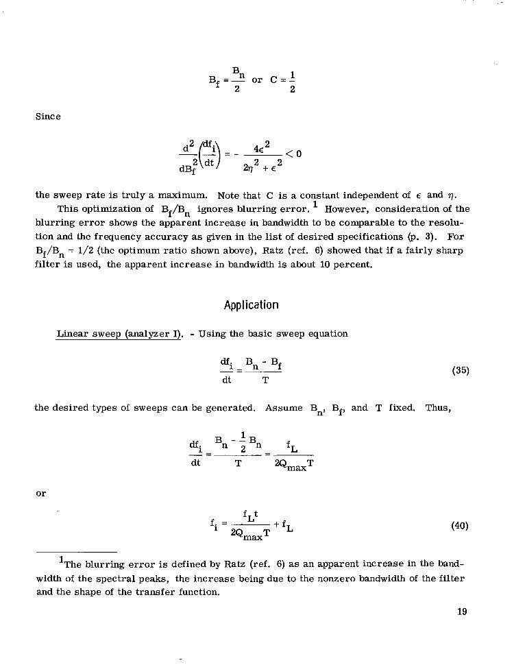
the sweep rate is truly a maximum.

blurring error shows the apparent increase in bandwidth to be comparable to the resolu- tion and the frequency accuracy as given in the list of desired specifications (p. 3). For Bf/Bn = 1/2 (the optimum ratio shown above), Ratz (ref. 6) showed that if a fair ly sharp filter is used, the apparent increase in bandwidth is about 10 percent.

Note that C is a constant independent of E and 7. This optimization of Bf/Bn ignores blurring error. However, consideration of the

Appl k a t ion

Linear sweep (analyzer I). - Using the basic sweep equation

dfi - Bn - Bf

dt T - - (35)

the desired types of sweeps can be generated. Assume Bn, Bf, and T fixed. Thus,

T QmmT dt

or

fLt

2QmaxT + fL f . =

1

‘The blurring error is defined by Ratz (ref. 6) as an apparent increase in the band- width of the spectral peaks, the increase being due to the nonzero bandwidth of the filter and the shape of the transfer function.

19

This equation is for a linear sweep spectrum analyzer, which for brevity is called ana- lyzer I in this report. Such a system has constant frequency resolution rather than constant-percent frequency resolution; thus, when analyzing vibration data, much time is wasted scanning the high-frequency end of the spectrum.

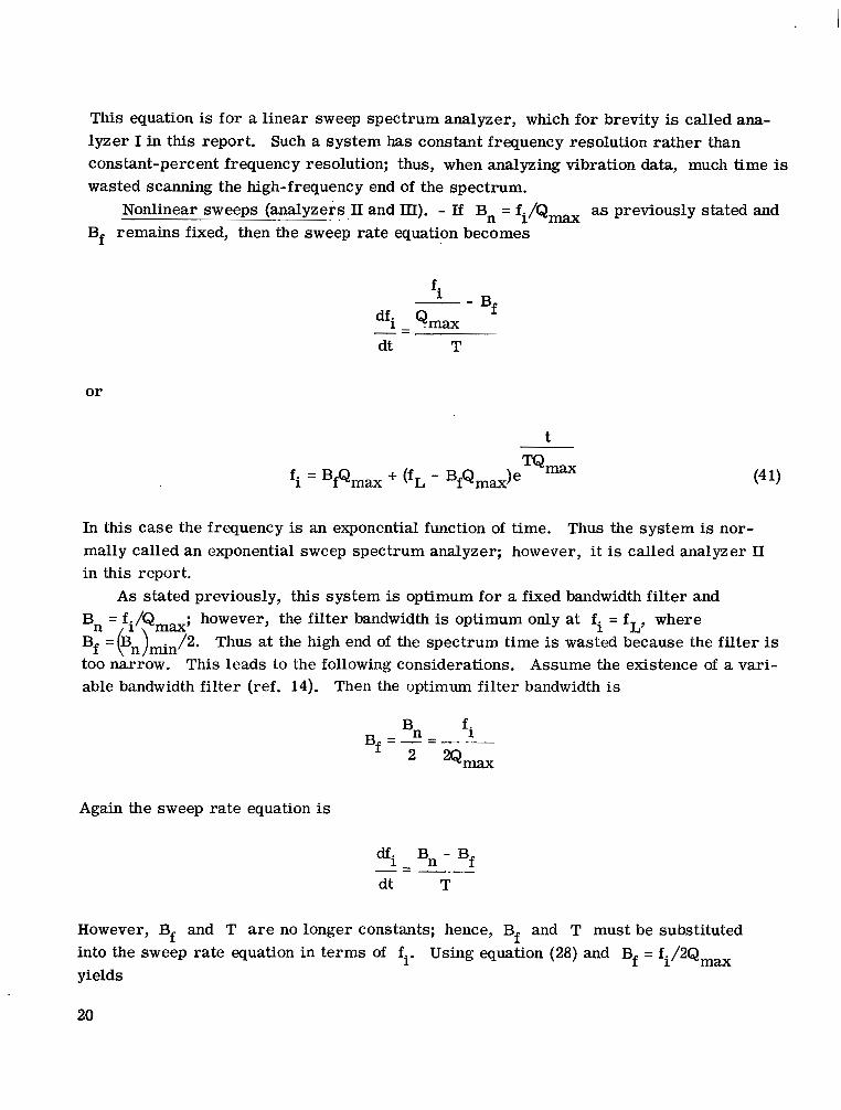
Bf remains fixed, then the sweep rate equation becomes Nonlinear sweeps (analyzers 11 and m). - If Bn = fi/Q- as previously stated and

Bf fi --

_ - ai - Qmax dt T

or

t

In this case the frequency is an exponential function of time. Thus the system is nor- mally called an exponential sweep spectrum analyzer; however, it is called analyzer I1 in this report.

As stated previously, this system is optimum for a fixed bandwidth filter and Bn = fi/Qmax; however, the filter bandwidth is optimum only at fi = fL, where Bf =(Bn)min/2. Thus at the high end of the spectrum time is wasted because the filter is too narrow. This leads to the following considerations. Assume the existence of a vari- able bandwidth filter (ref. 14). Then the optimum filter bandwidth is

Again the sweep rate equation is

dfi Bn - Bf

dt T

However, Bf and T are no longer constants; hence, Bf and T must be substituted into the sweep rate equation in terms of fi. Using equation (28) and Bf = fi/2Qmax yields

20

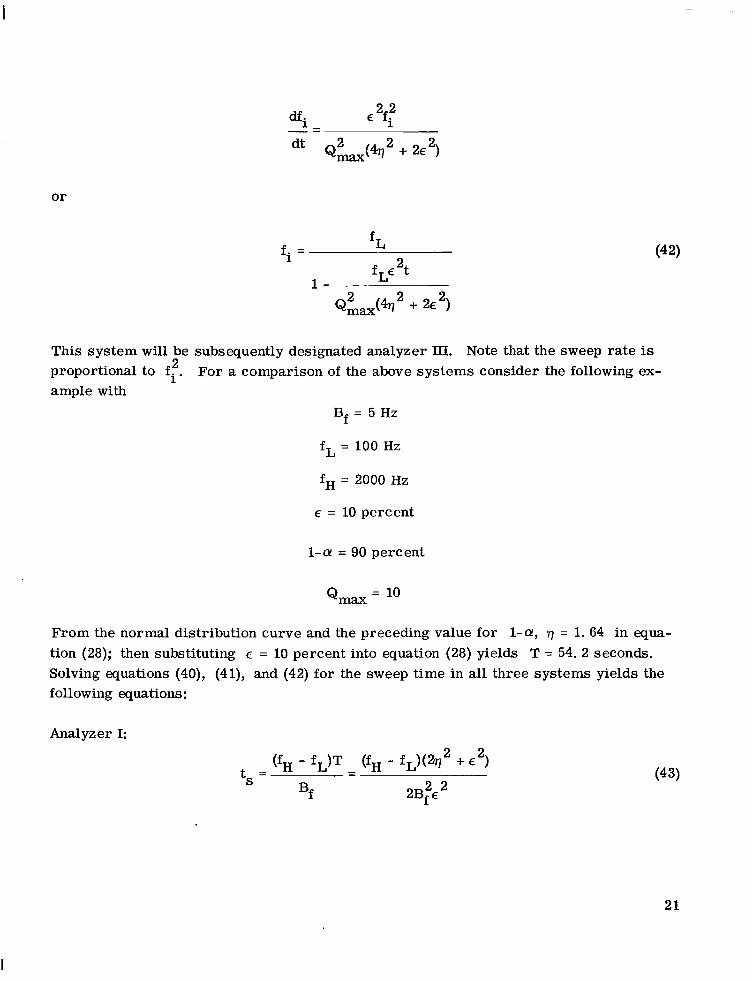
dt ( 4 q 2 + 2 € 2 ) Qmax

or

f . = f L 2 1

fLE t 1 - -

Qmax 2 (4q2+2E 2 )

This system will be subsequently designated analyzer III. 2 proportional to f i .

ample with

Note that the sweep rate is For a comparison of the above systems consider the following ex-

Bf = 5 Hz

fL = 100 HZ

fH = 2000 H Z

E = 10 percent

1-cr = 90 percent

From the normal distribution curve and the preceding value for 1-0, q = 1.64 in equa- tion (28); then substituting E = 10 percent into equation (28) yields T = 54. 2 seconds. Solving equations (40), (41), and (42) for the sweep time in all three systems yields the following equations:

Analyzer I:

(fH - fL)T

Bf

(fH - f ~ ) ( % ~ + E 2

2Bf 2 2 E

- t = - S (43)

2 1

Analyzer II:

Analyzer 111:

T In f~ - BfQmax

f~ - BfQmax ts = Qmax

2 26 Bf -

f L - BfQmax (44)

Substituting the appropriate values of fH, fL, T, Bf, Qmax , r ] , and E into equations (43), (44), and (45) yields

ts = 20 600 sec for analyzer I

ts = 1980 sec for analyzer II

ts = 1030 sec for analyzer III

The nonlinear sweep systems have much shorter sweep times than the linear system; however, none a r e feasible for real-time analysis of in-flight vibration data with the ac- curacy and sweep time requirements given in the INTRODUCTION. Clearly, i f ts is to be on the order of seconds, then accuracy, resolution, and confidence must be sacrificed. The following example was chosen to show to what extent the requirements must be de- graded to obtain sweep times on the order of seconds. Assume

r] = 0.84 (i. e.) 1-a! = 60 percent

fL = 100 HZ

fH = 2000 HZ

Qmax = 5

E = 40 percent

22

For analyzer I

ts = 91.6 sec

For analyzer I1

ts = 8.9 sec

For analyzer III

t = 4.6 sec S

In the first numerical example, the value for the degrees of freedom is 540; so there is no doubt about the normal distribution being a good approximation to the chi-square dis- tribution. mation gives

In the second example there a r e 9 degrees of freedom. The normal approxi-

1 [ - S(fc) -

5fc) P 0.60 < - < 1.40 = 0.60

The chi-square distribution gives

< 1.36 = 0.60 P 0. 598 <- 1 [ - S(fc) -

Qfc)

In view of the fact that E and (Y have been chosen to be 40 percent, the agreement be- tween the normal approximation and the chi-square distribution is more than adequate.

BANDWIDTH REQUIRED FOR TRANSMISSION OF SPECTRUMS

S i ng l e Spec t rum Ba ndwidt h Requ i remen t

Transmitting the spectrum of a signal rather than transmitting the time function will lead to a considerable saving in bandwidth. a resistor-capacitor (RC) averager on the power detector. Then, according to the dis- cussion following equation (13), RC = T/2.

Consider an airborne spectrum analyzer with

But according to equation (28)

23

2 2 27 + E n

T = 2Bf E '

I

For good response, the transmission channel should have a time constant shorter than the time constant of the data entering the channel; that is,

data time constant ~ > - . _ -

channel time constant (4 7)

The time constant of the channel response is l/n-Bc from equation (2 ) , where Bc is the transmitting channel bandwidth. Substituting these results into equation (47) yields

or

4rBfe 2

r (2q2 + E 2 )

B = C

This expression is valid for all three types of sweep functions. For analyzers I and 11, Bf is constant and equal to fL/2Q-, while for analyzer 111 the maximum value of Bf is used in equation (48); that is, Bf, max = fH/2Qmax. As a result, analyzer III re- quires substantially more bandwidth than analyzers I and II. The reason for the different bandwidth requirements is best understood by considering the power detector averaging time. In analyzers I and 11, the averaging time of the power detector is constant, while in analyzer III the averaging time is inversely proportional to frequency. Thus, a t the higher frequencies the power detector in analyzer 111 responds much faster than the de- tector in the other systems. Providing the bandwi-dth to transmit the more rapid changes in power level from analyzer 111 accounts for the increased bandwidth. The channel band- width Bc is calculated for all three types of analyzers using the values of Bf, E , and 77 of the previous sweep time examples. The values for Bc a re given in table I for the following conditions:

24

I

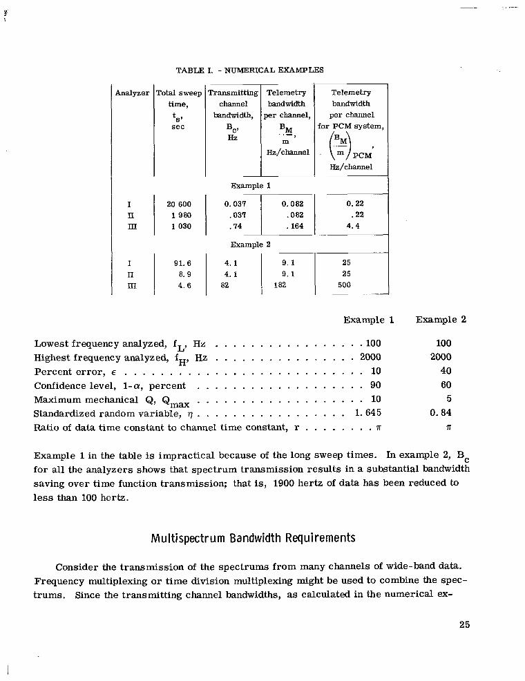
TABLE I. - NUMERICAL EXAMPLES

I II m

Analyzer

20 600 0.037 0.082 1980 1030 . 164

Total sweep time,

s ec tS ,

~

I I1 III

Transmitting channel

bandwidth,

&

91. 6 a. 9 4.6 a2

Telemetry bandwidth

per channel,

m &/channel

Telemetry bandwidth 1 per channel

for PCM system,

( 2 ) p c M &/channel

4.4

1 25 25 500

Example 1 Example 2

Lowest frequency analyzed, fL, Hz . . . . . . . . . . . . . . . . . 100 100 Highest frequency analyzed, fH, Hz . . . . . . . . . . . . . . . . 2000

Maximummechanical Q, Qmax . . . . . . . . . . . . . . . . . . . 10 5

2000 Percent error, E . . . . . . . . . . . . . . . . . . . . . . . . . . . 10 40 Confidence level, 1-a, percent . . . . . . . . . . . . . . . . . . . 90 60

Standardized random variable, q . . . . . . . . . . . . . . . . . 1.645 0.84 Ratio of data time constant to channel time constant, r . . . . . . . . 71 ‘IT

Example 1 in the table is impractical because of the long sweep times. In example 2, Bc for all the analyzers shows that spectrum transmission results in a substantial bandwidth saving over time function transmission; that is, 1900 hertz of data has been reduced to less than 100 hertz.

Mu 1 ti spect r u m Bandwidth Req ui r e me nts

Consider the transmission of the spectrums from many channels of wide-band data. Frequency multiplexing or time division multiplexing might be used to combine the spec- trums. Since the transmitting channel bandwidths, as calculated in the numerical ex-

25

amples, are so small, frequency stacking of the spectrum channels would be inefficient. More bandwidth would be used for channel separation than for information, and narrow, complex filters would be required. Time division multiplexing is more easily imple- mented.

Consider the following sampling method. Assume each spectrum analyzer output to be band limited to frequencies less than Bc. Then from sampling theory, (ref. 12), the theoretical minimum sampling rate is 2B Thus, to multiplex m spectrum channels, 2mBc samples per second are required.2C'The amplitudes of the 2mBc samples per sec- ond for m spectrum channels can be transmitted with an accuracy of about 3 percent; that is, e -3' by using a telemetry channel whose bandwidth is calculated from

3 5 1 3. 5 (channel time constant) = - = - aBM 2mBc

or

BM=- 7mc 71

(49)

The quantity %/m, the telemetry bandwidth per spectrum channel, may be used as a figure of merit for comparisons to other data transmission systems:

2 2 2 m 277 + E m

Values of BM/m were calculated for the two examples, and the results are given in table I. These results show that even after multiplexing, a large bandwidth saving still remains.

2The use of the theoretical minimum sampling rate based on the frequency limit Bc

The cut-off frequency of is sufficient in a practical system because of the frequency-limiting effects of the RC averager used on the power detector of the spectrum analyzer. the RC averager is B,/a. Thus, the frequency components in the analog signal repre- senting the spectrum are attenuated at frequencies above Bc/n. The lower frequency components of the signal, which comprise the major part of the signal, a r e sampled many times per cycle, which in a practical system yields good reproduction of the sampled spectrum.

26

I --.----... 1...-1.-.1.11--111..111111.1111111II.IIIII.II111II 11111111111111111 I 1111111111 I1 I I I I II I l lrl I I I I I I I I I I I I I Ill I I I I I I II

I

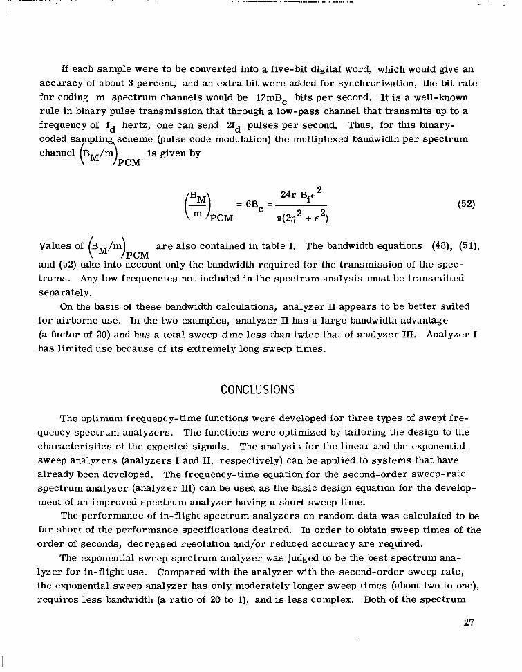
If each sample were to be converted into a five- bit digital word, which would give an accuracy of about 3 percent, and an extra bit were added for synchronization, the bit rate for coding m spectrum channels would be 12mBc bits per second. It is a well-known rule in binary pulse transmission that through a low-pass channel that transmits up to a frequency of fd hertz, one can send 2fd pulses per second. Thus, for this binary- coded sampling. scheme (pulse code channel B /m is given by ( )PCM

modulation) the multiplexed bandwidth per spectrum

2 24r Bfe = 6Bc =

n(2q2 + E2)

(521

Values of kM/m) are also contained in table I. The bandwidth equations (48), (51), PCM

and (52) take into account only the bandwidth required for the transmission of the spec- trums. Any low frequencies not included in the spectrum analysis must be transmitted separately.

for airborne use. In the two examples, analyzer 11 has a large bandwidth advantage (a factor of 20) and has a total sweep time less than twice that of analyzer LZI. Analyzer I has limited use because of its extremely long sweep times.

On the basis of these bandwidth calculations, analyzer 11 appears to be better suited

CONCLUSIONS

The optimum frequency-time functions were developed for three types of swept fre- quency spectrum analyzers. The functions were optimized by tailoring the design to the characteristics of the expected signals. The analysis for the linear and the exponential sweep analyzers (analyzers I and 11, respectively) can be applied to systems that have already been developed. The frequency-time equation for the second-order sweep-rate spectrum analyzer (analyzer ITI) can be used as the basic design equation for the develop- ment of an improved spectrum analyzer having a short sweep time.

The performance of in-flight spectrum analyzers on random data was calculated to be far short of the performance specifications desired. In order to obtain sweep times of the order of seconds, decreased resolution and/or reduced accuracy a r e required.

The exponential sweep spectrum analyzer w a s judged to be the best spectrum ana- lyzer for in-flight use. Compared with the analyzer with the second-order sweep rate, the exponential sweep analyzer has only moderately longer sweep times (about two to one), requires less bandwidth (a ratio of 20 to l), and is less complex. Both of the spectrum

27

analyzers with time-dependent sweep rates have sweep times about 10 times shorter than the constant sweep rate analyzer.

Finally, the bandwidth per channel was calculated for the transmission of spectrums. Spectrum analysis showed substantial bandwidth savings over the transmission of wide- band data (at least 75 to 1). Many channels of spectrums can be transmitted over one wide-band channel of an IRIG FM/FM system.

Lewis Research Center, National Aeronautics and Space Administration,

Cleveland, Ohio, June 20, 1966, 125- 24-03-03- 22.

28

APPENDIX - SYMBOLS

transmitting channel bandwidth for one channel of continuous spectrum infor- BC

Bf

BM

mation

effective filter bandwidth (bandwidth of the ideal rectangular filter that passes the same power as the real filter when both are excited by white noise)

telemetry bandwidth for m channels of sampled spectrums

E\ multiplexed bandwidth per spectrum channel for PCM system ' 'PCM

Bn minimum resolvable spectrum peak with center frequency fi

ratioof B to Bn,min

statistical expected value of y

statistical second moment of y

lower and upper frequency limits on effective bandwidth of analyzing filter

analyzing filter center frequency

highest frequency to be analyzed

signal frequency being analyzed

f C

E[Yl

E[Y21

fa9 f b

f C

fH

fi

- sweep rate dt

lowest frequency to be analyzed f L

mixing frequency

sweep rate constant

fS

K1

m number of channels

N number of samples taken to determine sample variance

numerical constant that allows adequate filter response for periodic signals

number of independent samples obtainable from band-limited white noise

N1

n

29

'[a < y < b] probability of a < y < b - - - - average power in x(t) contained between frequencies fa and fb

average power out of filter of bandwidth Bf, spanning fa to fb

probability distribution of x(t)

mechanical Q

autoc or r elation function

time constant of resistor-capacitor averaging circuit

ratio of data time constant to channel time constant

power spectral density

exact value of power spectral density at fc

estimated value of power spectral density at fc

estimated value of average power spectral density between frequencies fa and fb

lower and upper limits on confidence interval

sample variance

limit on integrations with respect to time; also used as averaging time for power detector

time constant of filter response to sine wave

detector averaging time

signal period for periodic signals

time

total sweep time

variance of x(t)

normal random variable with mean p and standard deviation u

specific values of chi-square random variable; the values a r e those which give the desired confidence level

signal (random o r periodic)

filter output

standardized normal random variable with zero mean and a standard deviation of one

fraction of measured values of the power spectral density that will lie outside the confidence interval

percent e r ror

standardized random variable that gives desired confidence level

mean value

true variance

lead time in autocorrelation computation

chi-square random variable with N- 1 degrees of freedom

Subscripts :

max maximum

min minimum

31

REFERENCES

1. Roche, A. 0. : The Use of Double Sideband Suppressed Carrier Modulation as a Sub- carrier for Vibration Telemetry. Proceedings of the National Telemetering Con- ference, June 2-4, 1964, Western Periodicals Co., 1964.

2. Frost, Walter 0. ; and King, Alin B. : SS-FM A Frequency Division Telemetry Sys- tem with High Data Capacity. Paper presented at the National Symposium on Space Electronics and Telemetry, IRE, 1959.

3. Tukey, J. W. ; and Hamming, R. W. : Measuring Noise Color 1. Bell Telephone Laboratories, Murray Hill, New Jersey, 1951.

4. Tukey, John W. : The Sampling Theory of Power Spectrum Estimates. Paper pre- sented at the Symposium on Applications of Autocorrelation Analysis to Physical Problems, Woods Hole, Mass., June 13-14, 1949. Office of Naval Research, Dept. of the Navy, 1949.

5. Chang, S. S. L. : On the Filter Problem of the Power-Spectrum Analyzer. IRE Proc., vol. 42, no. 8, Aug. 1954, pp. 1278-1282.

6. Ratz, Alfred G. : Telemetry Bandwidth Compression Using Airborne Spectrum Ana- lyzers. IRE Proc., vol. 48, no. 4, Apr. 1960, pp. 694-702.

7. Bendat, Julius S. ; and Piersol, Allan G. : Design Considerations and Use of Analog Power Spectral Density Analyzers. Measurement Analysis Corp. , printed by Honeywell, Denver Division, 1964.

8. Wylie, Clarence R., Jr. : Advanced Engineering Mathematics. McGraw-Hill Book Co., Inc., New York, 1951.

9. Davenport, Wilbur B., Jr. ; and Root, William L. : An Introduction to the Theory of Random Signals and Noise. McGraw-Hill Book Co., Inc., 1958.

10. Bendat, Julius S. : Principles and Applications of Random Noise Theory. John Wiley & Sons, Inc., 1958.

11. Lee, Yuk Wing: Statistical Theory of Communications. John Wiley & Sons, Inc., 1960.

12. Goldman, Stanford: Information Theory. Prentice-Hall, 1953, ch. 2.

13. Fraser, D. A. S. : Statistics, an Introduction. John Wiley and Sons, Inc., 1958,

14. Valley, George E., Jr. ; and Wallman, Henry, eds. : Vacuum Tube Amplifiers.

Ch. 8, pp. 165-213.

McGraw-Hill Book Co., Inc., 1948, pp. 384-408.

32 NASA-Langley, 1966 E- 3299

“The aeronautical and space activities of the United States shall be conducted JO as to contribute . . . to the expansion of human knowl- edge o f phenomena in the atmosphere and space. The Administration shall provide for the widest practicable and appropriate dissemination of information concerning its activities and the results thereof.”

-NATIONAL AERONAUTICS AND SPACE ACT OF 1958

NASA SCIENTIFIC AND TECHNICAL PUBLICATIONS

TECHNICAL REPORTS: important, complete, and a lasting contribution to existing knowledge.

TECHNICAL NOTES: of importance as a contribution to existing knowledge.

TECHNICAL MEMORANDUMS: Information receiving limited distri- bution because of preliminary data, security classification, or other reasons.

CONTRACTOR REPORTS: Technical information generated in con- nection with a NASA contract or grant and released under NASA auspices.

TECHNICAL TRANSLATIONS: Information published in a foreign language considered to merit NASA distribution in English.

TECHNICAL REPRINTS: Information derived from NASA activities and initially published in the form of journal articles.

SPECIAL PUBLICATIONS: Information derived from or of value to NASA activities but not necessarily reporting the results .of individual NASA-programmed scientific efforts. Publications include conference proceedings, monographs, data compilations, handbooks, sourcebooks, and special bibliographies.

Scientific and technical information considered

Information less broad in scope but nevertheless

I .

Details on the availability o f these publications may be obtained from:

SCIENTIFIC AND TECHNICAL INFORMATION DIVISION

N AT1 0 NAL AERONAUTICS AND SPACE ADM I N ISTRATI 0 N

Washington, D.C. PO546