Soft ComputDOI 10.1007/s00500-015-1862-7

METHODOLOGIES AND APPLICATION

Design and theoretical analysis of virtual machine placementalgorithm based on peak workload characteristics

Weiwei Lin1 · SiYao Xu1 · Jin Li2 · Lingling Xu1 · Zhiping Peng3

© Springer-Verlag Berlin Heidelberg 2015

Abstract Virtual machine (VM) placement is a fundamen-tal problem about resource scheduling in cloud computing;however, the design and implementation of an efficient VMplacement algorithm are very challenging. To better multi-plex and share physical hosts in the cloud data centers, thispaper presents a VM placement algorithm based on the peakworkload characteristics, which models the workload char-acteristics of VMs with mathematical method, and measuresthe similarity of VMs’ workload with VM peak similarity.Avoiding virtual machines whose workload has high corre-lation are placed together, it places the virtual machines withpeak workload staggering at different time together, whichachieves better VM consolidation through VM peak simi-larity. This paper focuses on the mathematical analysis ofVM peak similarity, and proves that compared to cosine-similarity method and correlation-coefficient method, peak-similarity method is better theoretically. Finally, numeri-cal simulations and algorithm experiments show that ourproposed peak-similarity-based placement algorithm out-performs the random placement algorithm and correlation-coefficient-based placement algorithm.

Keywords Cloud computing · Peak characteristics ·Similarity · Placement of virtual machine · Theory proof

Communicated by V. Loia.

B Weiwei Linlinww@scut.edu.cn

1 School of Computer Science and Engineering, South ChinaUniversity of Technology, Guangzhou, China

2 Department of Computer Science, Guangzhou University,Guangzhou, China

3 College of Computer and Electronic Information, GuangdongUniversity of Petrochemical Technology, Maoming, China

1 Introduction

Cloud computing (Foster et al. 2008; Chen et al. 2009; Linet al. 2012) is one of the most hot topics in recent years. Vir-tualmachine placement is a fundamental problemof resourcemanagement in cloud data center and, also, an importantresearch direction of cloud computing resource scheduling.Reasonable virtual machine placement and scheduling algo-rithm can improve resource utilization of cloud data centersand reduce operation costs. Research and implementationof effective virtual machine placement algorithm can buildenergy-efficient cloud data center, which is conducive to theapplication and popularization of cloud computing technol-ogy.

On the problem of virtual machine placement, domes-tic scholars have conducted a lot of research in recentyears. Influential research is analyzed as follows. Paper (Weiet al. 2013) proposed a consolidation algorithm based onvirtual machine workload forecasting. Forecasting modelemploys autoregressive model and exponential smoothingmodel. Simulation is conducted by CloudSim and the resultsshow that the algorithm can effectively reduce the num-ber of physical servers, the number of migration virtualmachines and SLA violation. To balance energy efficiencywith network performance of cloud data center, Dong et al.(2014) proposed a new virtual machine placement schemethat can achieve two objectives. One is to minimize the num-ber of activating physical machines and network devices toreduce the energy consumption, and the other is to mini-mize the maximum link utilization to improve the networkperformance. Authors designed a two-stage heuristic algo-rithm to accelerate problem solving and simulation resultsshow that the proposed virtual machine placement methodachieves good results. Aiming at the virtual machine place-ment optimization problem, Liu et al. (2012) modeled the

123

W. Lin et al.

energy consumption of heterogeneous data center and pro-posed an energy-aware virtual machine placement intelligentoptimization algorithmbased ondiscrete particle swarmopti-mization. A novel two-dimension particle encoding methodwas presented. An adaptive weight distribution mechanismwas introduced to update the particle velocity, and then anenergy-aware local fitness first mechanism was designedto update the particle location to improve the efficiency.The comparison of simulation experiments indicates that theproposed algorithm significantly improves the server utiliza-tion, saves more power and reduces the operation cost ofdata centers. Considering the resource consumption over-head caused by the waiting of virtual machines for serverresource scheduling, Li et al. (2014) researched on theresource-scheduling-waiting-aware virtual machine consol-idation. The study theoretically and experimentally provesthat under realistic constraints, there exists server resourceadditional overhead caused by the virtual machine waitingfor resource scheduling. This overhead remains steady as thenumber of consolidating VMs grows. Our team conducted alot of research in the areas of resource management aboutcloud computing and VM resource scheduling optimiza-tion (Lin et al. 2011, 2012, 2013, 2015; Chen et al. 2014).In the paper (Lin et al. 2013), we modeled the energy opti-mization problem of virtual machine resource scheduling ina heterogeneous cloud data center. By solving the constraintsatisfaction problem, the optimized allocation scheme mini-mizing energy consumption in virtualized cloud data centersis also obtained. Based on the optimized allocation scheme,an energy-efficient resource allocation algorithm, dynamicpower (DY), which takes into account the heterogeneityof resources, was proposed. The performance of algorithmwas evaluated using Choco. Experimental results show that,compared with first-fit decreasing (FFD), best-fit decreas-ing (BFD) and minimizing the number of physical machines(MinPM), the proposed algorithm (DY) has less energy con-sumption. We introduced constraint satisfaction problemsto model cloud virtual machine placement problem in thepaper (Lin et al. 2015), and implemented Choco-based vir-tual machine resource allocation algorithm. The comparisonexperiment with IFFD, IBFD algorithms shows that virtualmachine resource allocation algorithm based on Choco hasgreatly improved, but costs a longer running time. To thisend, equivalence optimizationmethod for resource allocationwas further proposed to accelerate the constraint resourceallocation solving. When searching for resource allocation,equivalent resource is pruned, reducing the space for solv-ing resource allocation and accelerating the solution to theresource allocation model. Experimental results show thatequivalent optimization method proposed greatly decreasesthe time to solve resource allocation.

Worldwide, many scholars adopted some heuristic algo-rithm to realize virtual machine placement (Nakada et al.

2009; Hirofuchi et al. 2013; Agrawal et al. 2009; Gaoet al. 2013; Hu et al. 2010; Xu et al. 2014; Wang et al.2014). Paper (Nakada et al. 2009) used the genetic algorithmbased on the number of physical machines, Service Levelagreements (Service Level Agreement), and virtual machinemigration times as optimization targets to find the solu-tion, but did not consider physical machine’s load balance.Paper (Hirofuchi et al. 2013) realized the cloud resource allo-cation bymodeling the placement problembased onCPUandmemory constraint, which considered the virtual machineconfiguration andmigration time. Paper (Agrawal et al. 2009)solved the problem of server consolidation using groupinggenetic algorithm with the constraint that part of virtualmachines is incompatible. Paper (Gao et al. 2013) presented aserver load balancing method based on ant colony algorithm.Because each ant only updates the local pheromone after theestablishment of their result sets, algorithm converges in slowspeed. A load balancing VM placement algorithm based ongenetic algorithm was put forward in paper (Hu et al. 2010).Themethod combines the state of virtual machine placed andhistorical data, targeting system load balance optimization.With respect to non-heuristic algorithm, Chen et al. (2011)presented a novel effective vm sizing method. Effectivesizing decides a VM’s resource demand by statistical mul-tiplexing. The effective size consists of two parts: intrinsicdemand and correlation-aware demand. The server consoli-dation is formulated as a stochastic bin packing problem.Kimet al. (2013) defined a new function for measuring the corre-lation of two virtual machines.Whereby, this virtual machineconsolidation achieves energy savings. The effectiveness ofthe solution was validated using (1) multiple clusters of real-life scale-out application workloads-based web search and(2) utilization traces obtained from real-data center setups.According to the experiments, the proposed solution providesup to 13.7% energy savings with up to 15.6% improvementof quality of service (QoS) compared to existing correlation-aware VM allocation methods for datacenters. In addition,paper (Meng et al. 2010) proposed a model for estimatingthe aggregate size of multiplexed VMs. The model explainsthat the historical workload can be divided into tendency partand random part, forecasts the workload with time sequence,and selects high complementary VM pairs according to thecorrelation coefficient matrix. It achieves VM consolidation,but the consolidation is limited to pair.

Although domestic and foreign scholars conducted a lot ofresearch on VM scheduling andmultiplexing in recent years,however, the current algorithm still has some shortcomings.Different from existing research, from the perspective ofmathematical modeling about virtual machine’s workloadcharacteristics, this paper presents a VM placement algo-rithm based on the peak workload characteristics, whichmeasure the similarity of VMs’ peak workload character-istics with peak similarity. Avoiding virtual machines whose

123

Design and theoretical analysis of virtual machine placement algorithm based on peak workload. . .

workload has high correlation are placed together, it placesthe virtual machines with peak workload staggering at differ-ent time together, so as to better multiplex physical hosts andimprove the utilization of resource significantly. Moreover,we theoretically proved that peak similarity is more univer-sal and accuracy as comparedwith the traditional parameters.Peak similarity can overcome the weakness that the descrip-tion of virtual machine’s workload characteristics describedby traditional parameter is inadequate and inaccurate. Thealgorithm better realizes resource multiplying and sharingof virtual machine, and improves the resource utilizationin cloud data center. The rest of the paper is organized asfollows. In Sect. 2, we introduce the basic idea and the math-ematical model of virtual machine placement algorithm. Thethird section focuses on the analysis of the peak similaritytheoretically, and compares it with cosine similarity and cor-relation coefficient. In Sect. 4, we give numerical simulationand simulation experiment results. Finally, it is the summaryand the prospect of the future work.

2 Ideas and model

2.1 Basic idea of algorithm

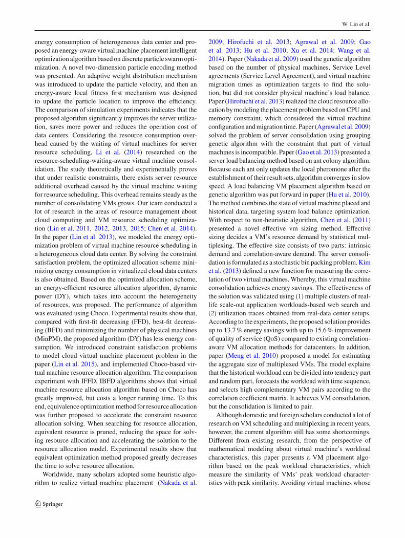
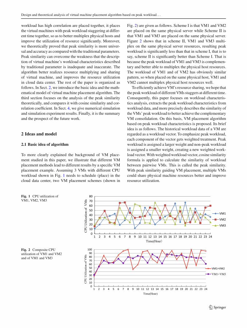
To more clearly explained the background of VM place-ment studied in this paper, we illustrate that different VMplacement methods lead to different results by a specific VMplacement example. Assuming 3 VMs with different CPUworkload shown in Fig. 1 needs to schedule (place) in thecloud data center, two VM placement schemes (shown in

Fig. 2) are given as follows. Scheme I is that VM1 and VM2are placed on the same physical server while Scheme II isthat VM1 and VM3 are placed on the same physical server.Figure 2 shows that in scheme II, VM1 and VM3 multi-plex on the same physical server resources, resulting peakworkload is significantly less than that in scheme I, that is tosay, scheme II is significantly better than Scheme I. That isbecause the peak workload of VM1 and VM3 is complemen-tary and better able to multiplex the physical host resources.The workload of VM1 and of VM2 has obviously similarpattern, so when placed on the same physical host, VM1 andVM2 cannot multiplex physical host resources well.

To efficiently achieveVM’s resource sharing,we hope thatthe peakworkload of differentVMs staggers at different time.Consequently, this paper focuses on workload characteris-tics analysis, extracts the peak workload characteristics fromworkload data, and more precisely describes the similarity oftheVMs’ peakworkload to better achieve the complementaryVM consolidation. On this basis, VM placement algorithmbased on peak workload characteristics is proposed. Its briefidea is as follows. The historical workload data of a VM areregarded as a workload vector. To emphasize peak workload,each component of the vector gets weighted treatment. Peakworkload is assigned a larger weight and non-peak workloadis assigned a smaller weight, creating a new weighted work-load vector.Withweightedworkload vector, cosine similarityformula is applied to calculate the similarity of workloadbetween pairwise VMs. This is called the peak similarity.With peak similarity guiding VM placement, multiple VMscould share physical machine resources better and improveresource utilization.

Fig. 1 CPU utilization ofVM1, VM2, VM3

Fig. 2 Composite CPUutilization of VM1 and VM2and of VM1 and VM3

123

W. Lin et al.

2.2 Mathematical model of the algorithm

To study the characteristics of the peak workload of VM,we first define peak workload and off-peak workload.This paper presents two approaches of definition for peakworkload.

Definition 1 (Fixed boundary model) Within a certain timeinterval, let Xi denote the resource utilization at time ti .GivenP(0 < P < 1), if

Xi > P,

then the point (ti , Xi ) is called peak point, otherwise knownas non-peak point.

In particular, within a period of timeworkload of VMmayhave been small, no more than P , then the VM does not haveany peak points. Conversely, if a VM sustained relativelylarge workload, then the workload points of the VM may beall peak points with a small P .

Definition 2 (Fixed ratio model)Within a certain time inter-val, let X denote the average resource utilization during thisperiod of time. Given a ratio ρ(ρ > 1), if

Xi > ρ X ,

then the point (ti , Xi ) is called peak point, otherwise knownas non-peak point.

Ifρ is large, the extreme situation is thatρ X is even greaterthan 1, then it will cause no peak point. Yet since X is greaterthan 1, non-peak points definitely exist.

Here, the value of P and ρ is defined by our own. The liney = P , y = ρ X is both referred to as the peak-boundaryline.

After differentiating between peak point and non-peakpoint, we need to compare the similarity of two VMs’ work-load, especially whether their peak workload occurs at neartime or not. Themore overlapping the peak period, the higheris the similarity. Therefore, this paper introduces the cosinesimilarity computational formula. To emphasize the charac-teristics of peak points, we assign larger weights to the peakpoints, and we get the formula of weighted peak similarity(peak similarity for short).

sim<X,Y> =∑n

i=1 uivi XiYi√∑n

i=1 ui2Xi

2 ∑ni=1 vi 2Yi 2

(2.1)

where Xi ,Yi denote the workload of VM A and VM B,respectively, i.e., CPU utilization at time ti . ui denotes theweight of Xi , similarly, vi denotes the weight of Yi . Thevalue of weight depends on whether the workload point ispeak point or not. First, given a total weight Q for peak

points, the total weight for non-peak points is (1 − Q). Fornon-peak points, the weights share the total weight (1 − Q)

equally, i.e., if there exist d(d < n) non-peak points, theweights of these d non-peak points are all 1−Q

d . For peakpoints, the weights are prorated according to the portionthat the peak exceeds the peak-boundary line. For instance,given that the peak-boundary line is y = P , the weight ofpeak point Xi equals Q

Xi−P∑Xi∈H(X) (Xi−P)

where H(X) is the

peak point set. We also call Xi as a peak point for conve-nience.

Under special circumstances, when peak-boundary line issufficiently large, all the points of X are non-peak points. Theweights of non-peak points, of all the points simultaneously,are all equal to 1

n . We could comprehend under this situationQ is 0. When peak-boundary line is sufficiently small, all thepoints of X are peak points. The weights of peak points are

Xi−P∑Xi∈H(X) (Xi−P)

. Similarly, we could comprehend under this

situation Q is 1.Suppose y = E is the peak-boundary line, function (2.2)

is defined as an auxiliary function for deciding the work-load point whether a non-peak point or not.

∑ni=1 ω(Xi , P)

represents the number of non-peak points.

ω(x, E) ={1, x ≤ E0, x > E

(2.2)

The formula of weight can be written as:

u(x) ={Q x−P∑

Xi∈H (Xi−P)

(1 − Q) 1∑n1 ω(Xi ,P)

(2.3)

By Eq. (2.3), the weight of each point can be calculated.With the weights substituting into Eq. (2.1), we get the sim-ilarity between two VMs’ workload.

3 Theoretical analysis and comparison

3.1 Mathematical analysis of peak similarity

Peak similarity is essentially cosine similarity. The differenceis that peak similarity assigns a greater weight to peak point,but this statement is very general. In this section, we presentthe mathematical analysis of peak similarity and figure outthe scope and limitation of peak similarity on describing thedifference of workload.

cos θ =∑n

i=1 XiYi√∑n

i=1 X2i

∑ni=1 Y

2i

Cosine similarity is a measurement of the angle betweentwo vectors. The value has no concern with the length of

123

Design and theoretical analysis of virtual machine placement algorithm based on peak workload. . .

the two vectors, but only concerns the directions of those.That is to say, the vector X lengthened or shortened doesnot change its cosine with other vectors. Consider the vectorX = (x1, x2, . . . , xn) and vector X0 = ( x1n , x2

n , . . . , xnn ),

Y = (y1, y2, . . . , yn). The vectors we are discussing, if notspecified, are all referred to the workload vectors, i.e., vector(x1, x2, . . . , xn) that satisfies 0 < xi < 1, i = 1, 2, . . . , n.

cos(X0,Y ) =∑n

i=1xin yi√∑n

i=1xin2 ∑n

i=1 y2i

=1n

∑ni=1 xi yi√

1n2

∑ni=1 x

2i

∑ni=1 y

2i

=∑n

i=1 xi yi√∑ni=1 x

2i

∑ni=1 y

2i

= cos<X,Y>.

(3.0)

From the calculation of formula 3.0, we can see that thevector X0 is a special workload vector under the situation thatall the workload points are non-peak points and it is gainedfrom each component of X multiplied by the weight. Thatmeans, cosine similarity is the peak similarity under spe-cific circumstance that the peak-boundary line is sufficientlylarge.

We call the process that X = (x1, x2, . . . , xn) is convertedinto X ′ = (u1x1, u2x2, . . . , unxn) as peak transform. ui istheweight of xi in the peak similarity formula. Formulizationis X ′ = PE(X).

The concept of “rearrangement” is mentioned later, soseveral definitions are given here first.

Permutation In general, putting n numbers in a certainorder in a row is called a permutation of n numbers.

These n numbers may be equal. A permutation can bedenoted simply by a permutation vector, such as (0.2, 0.4,0.2). It is a permutation comprising 0.2, 0.2, and 0.4.

Re-permutation Rearranging the numbers of a permuta-tion in a different order is called re-permutation.

Vector re-permutationmeans rearranging each componentof the vector to get a new vector.

Synchronization re-permutation It is a two-vectors’ re-permutation that keeps the correspondence between twovectors’ components and queues in the same manner. Forexample, supposed vector X = (0.1, 0.2, 0.4, 0.15), Y =(0.3, 0.2, 0.1, 0.25), holding the correspondence relation-ship between X (i) and Y (i), i = 1, 2, 3, 4, rearrange thevector X , Y . Exchange the first component and the thirdcomponent and exchange the second component and thefourth component.We get vectors X ′ = (0.4, 0.15, 0.1, 0.2),Y ′ = (0.1, 0.25, 0.3, 0.2). This is a synchronization re-permutation of vector X and Y .

Based on formulas 3.1, 3.2, 3.3, the synchronization re-permutation of vector X , Y does not change their cosine

similarity, correlation coefficient and peak similarity.

cos θ =∑n

i=1 xi yi√∑ni=1 x

2i

∑ni=1 y

2i

(3.1)

r =∑n

i=1 (xi − x)(yi − y)√∑n

i=1 (xi − x)2∑n

i=1 (yi − y)2(3.2)

γ =∑n

i=1 uivi xi yi√∑ni=1 (ui xi )2

∑ni=1 (vi yi )2

(3.3)

Theorem 1 Vector X ′ = (x ′1, x

′2, . . . , x

′n) is a re-permutati-

onof vector X = (x1, x2, . . . , xn). Suppose I = (c, c, . . . , c)∈ Rn, and c is a constant, then for any P, Q,

sim<X, I> ≡ sim<X ′, I>.

Owing to commutative law of addition, this theorem isobvious.

Theorem 2 If the vector X = (x1, x2, . . . , xn) satisfies: for∀i �= j , i, j = 1, 2, . . . , n,

xi �= x j

then there do not exist two vectors Y, Z such that Y �= Z, forany P, Q,

sim<X,Y> ≡ sim<X, Z>.

Theorem 3 Set R = {1, 2, . . . , n}, and Gi (i = 1, 2, . . . , k)are mutually disjoint subsets of R such that there exist somecomponents of vector X (x1, x2, . . . , xn) such that xi = ciand ci is a constant, j ∈ Gi , 0 < ci < 1, cs �= ct , ∀s �= t ,s, t = 1, 2, . . . , k. Let Y (i) denote the vector comprising ofcomponents whose subscript belongs to Gi . Z (i) is similar.Then, for any P, Q,

sim<X,Y> ≡ sim<X, Z>.

iff (1) ∀i , (i = 1, 2, . . . , k), Z (i) is a re-permutation of Y (i);(2) ∀ j ∈ R\⋃k

i=1 Gi , zi = yi .

Here is a simple example for Theorem 3.3. X =(0.2, 0.2, 0.2, 0.3, 0.1, 0.4, 0.1); Y = (0.3, 0.5, 0.1, 0.4,0.2, 0.1, 0.3); Z = (0.1, 0.3, 0.5, 0.4, 0.3, 0.1, 0.2). For X ,there are some components that equal 0.2 or 0.1. Here, k = 2.G1 = {1, 2, 3}, which means that x1 = x2 = x3 = c1 = 0.2.G2 = {5, 7}, which means that x5 = x7 = c2 = 0.1.Meanwhile, Y (1)= (0.3, 0.5, 0.1), Z (1)= (0.1, 0.3, 0.5). Z (1)

is a re-permutation of Y (1). Similarly, Y (2) = (0.2, 0.3),Z (2) = (0.3, 0.2). Z (2) is a re-permutation of Y (2). x4 = 0.3,x6 = 0.4, on the other hand, y4 = z4 = 0.4; y6 = z6 = 0.1.Therefore, Y and Z satisfy the conditions of Theorem 3.3; we

123

W. Lin et al.

could draw the conclusion that for any P , Q, sim<X,Y> ≡sim<X, Z>.

Theorems 1, 2, and 3 tell us the identical conditions ofpeak similarity. In other words, when these conditions arenot satisfied, the peak similarity between workload vec-tors is not always equal. That means that peak similarityis capable of differentiating between two virtual machines’workload.

To prove these two theorems, three lemmas are givenfirst.

Lemma 1 X ′ = PE(X) = (u1x1, u2x2, . . . , unxn), Y ′ =PE(Y ) = (v1y1, v2y2, . . . .vn yn), then for any P, Q, X ′ ≡Y ′, iff X = Y .

Proof (I) Sufficiency: Since X = Y , X ′ ≡ Y ′ is obvious.(II) Necessity: Prove by contradiction. Suppose there exist

vectors X and Y such that X �= Y and for any P, Q,X ′ ≡ Y ′ , then ui xi = vi yi , i = 1, 2, . . . , n.Since X �= Y , there exists i0, xi0 �= yi0 . We might aswell set xi0 < yi0 .Let P = xi0 , then xi0 is a non-peak point, yi0 is a peakpoint. Let the number of non-peak points of X be d1 andthat of Y be d2. There exists at least a point yi0 that is apeak point of Y . Then, ui0 = 1−Q

d1, (when d1 < n) vi0 =

Qyi0−P

∑yi∈H(Y ) (yi−P)

. So, 1−Qd1

xi0 = Qyi0−P

∑yi∈H(Y ) (yi−P)

yi0 ,

thend1(yi0−P)

∑yi∈H(Y ) (yi−P)

yi0xi0

= 1−QQ . In this situation, Q has

only one solution.If all points of X are non-peak points when P = xi0 ,i.e., d1 = n, then ui0 = 1

n . Similarly,n(yi0−P)

∑yi∈H(Y ) (yi−P)

yi0xi0

= 1Q .

Also Q has only one solution.Therefore, the assumption does not hold.Consequently, there do not exist vectors X and Y suchthat X �= Y and for any P , Q, X ′ ≡ Y ′. That impliesthat if X ′ ≡ Y ′ for any P , Q, there must be X ≡ Y . �

Lemma 2 X ′ = PE(X) = (u1x1, u2x2, . . . , unxn), Y ′ =PE(Y ) = (v1y1, v2y2, . . . .vn yn). Given i , for any P, Q,ui ≡ vi , xi = yi and Y is a re-permutation of X.

Proof (I) Sufficiency:

1. When P ≥ xi , ui = 1−Qd1

, vi = 1−Qd2

, (d1 < n, d2 <

n), Since Y is a re-permutation of X , the numbers oftheir non-peak points are the same. Therefore, ui =vi . In particular, when d1 = n, d2 = n, ui = vi = 1

n .

2. When P < xi , ui = Q xi−P∑x j∈H(X) (x j−P)

, vi =Q yi−P∑

y j∈H(Y ) (y j−P). Since xi = yi , the numerators

of the two weights are equal. Y is a re-permutationof X , so for any P , Y and X have the same peakpoints. According to the commutative law of addi-

tion,∑

x j∈H(X) (x j − P) = ∑y j∈H(Y ) (y j − P),

thus ui ≡ vi .(II) Necessity: First if xi �= yi , set xi < yi , P = xi , then

ui = 1−Qd1

, vi = Q yi−P∑y j∈H(Y ) (y j−P)

. It is easy to know

that Q has only one solution. ui is not identicallyequal to vi , so xi = yi .

1. When P < xi , what we need to do is to com-pare

∑x j∈H(X) (x j − P),

∑y j∈H(Y ) (y j − P). Let

set Z = {z|z = xi or z = yi , i = 1, 2, . . . , n}. Setm = card(Z), then m ≥ n. Let the sorted elementsof set Z be z1, z2, . . . , zm .Let P in turn take P1 = z1 − ε, P2 = z2 − ε,…,Pm = zm − ε, Pm+1 = zm + ε, ε > 0. Let P1denote the numbers in interval (0, z1). Let P2 denotethe numbers in interval [z1, z2), and so on.Let Si (X) = ∑

x j∈H(X) (x j − Pj ), and Si (Y ) =∑

y j∈H(Y ) (y j − Pj ).When P = P1, All points of X,Y are peak points.S0(X) = ∑n

i=1 xi − nP0, S0(Y ) = ∑ni=1 yi − nP0.

X,Y should satisfy

n∑

i=1

xi =n∑

i=1

yi . (3.4)

When P = P2, if z1 is a component of X and not anycomponent of Y , i.e., there exists i0 such that z1 = xi0and for ∀i , yi �= z1, then

S1(X) = ∑

i �=i0

xi − (n − 1)P1,

S1(Y ) =n∑

i=1yi − nP1

∑

i �=i0

xi − (n − 1)P1 =n∑

i=1yi − nP1,

(3.5)

(3.4) subtracts (3.5), then we will derive that xi0 =P1 = z1 − ε and z1 = xi0 are contradictory. Thissituation does not meet the conditions.If there exists a subscript set of X : I1(X) = {i |xi =z1} and of Y : I1(Y ) = {i |yi = z1}, then

S1(X) = ∑

i /∈I1(X)

xi − (n − card(I1(X)))P1,

S1(Y ) = ∑

i /∈I1(Y )

yi − (n − card(I1(Y )))P1∑

i /∈I1(X)

xi − (n − card(I1(X)))P1∑

i /∈I1(Y )

yi − (n − card(I1(Y )))P1

(3.6)

(3.4) subtracts (3.6), then

123

Design and theoretical analysis of virtual machine placement algorithm based on peak workload. . .

∑

i∈I1(X)

xi − card(I1(X))P1

=∑

i∈I1(Y )

yi − card(I1(Y ))P1,

Namely,

card(I1(X))z1 − card(I1(X))P1= card(I1(Y ))z1 − card(I1(Y ))P1,

card(I1(X))ε = card(I1(Y ))ε.

Therefore, card(I1(X)) = card(I1(Y )).When P = Pi (i ≥ 3), the derivation process is thesame as that when P = P2. It also comes to a con-clusion that there must exist a component or somecomponents of both X and Y that equal to zi and thenumber of such components are equivalent. Thus, Yis a re-permutation of X .

2. When P ≥ xi , since Y is a re-permutation of X ,ui = vi .

In summary, that Y is a re-permutation of X is the nec-essary condition of ui = vi . �

Lemma 3 A > 0,C > 0, A2

B = C2

D B − D←−−→AB = C

D .

Proof (I) Sufficiency: B = D and AB = C

D yield A = C .

Therefore, A × AB = C × C

D , namely A2

B = C2

D .

(II) Necessity: B = D and A2

B = C2

D . yield A2 = C2. SinceA > 0 and C > 0, A = C . Thus, A

B = CD . �

The proof of Theorem 3.2 is as follows.

Proof Prove by contradiction. Suppose there exist vectors Yand Z such that Y �= Z and for any P, Q, sim<X,Y> ≡sim<X, Z>. Let

sim〈X,Y 〉 =∑n

i=1 uivi xi yi√∑ni=1 u

2i x

2i

∑ni=1 v2i y

2i

,

sim〈X, Z〉 =∑n

i=1 uiwi xi zi√∑n

i=1 u2i x

2i

∑ni=1 w2

i z2i

,

then for any P, Q,

∑ni=1 uivi xi yi√∑n

i=1 u2i x

2i

∑ni=1 v2i y

2i

=∑n

i=1 uiwi xi zi√∑n

i=1 u2i x

2i

∑ni=1 w2

i z2i

,

namely,

(∑n

i=1 uivi xi yi )2

∑ni=1 v2i y

2i

= (∑n

i=1 uiwi xi zi )2∑n

i=1 w2i z

2i

.

Firstly, consider the following equation:

∑ni=1 uivi xi yi

2

∑ni=1 v2i y

2i

=∑n

i=1 uiwi xi zi∑n

i=1 w2i z

2i

. (3.7)

Set it as a polynomial with respect to xi .

(

v1y1

2∑

i=1

w2i z

2i − w1z1

2∑

i=1

v2i y2i

)

u1x1

+(

v2y2

2∑

i=1

w2i z

2i − w2z2

2∑

i=1

v2i y2i

)

u2x2 + · · ·

+(

vn yn

2∑

i=1

w2i z

2i − wnzn

2∑

i=1

v2i y2i

)

unxn ≡ 0.

(3.8)

Since xi (i = 1, 2, . . . , n) does not equal to each other, byLemmas 1, ui xi is not identically equal to u j x j as long asi �= j . Consequently, the n terms of (3.5) cannot combine.

Next, we will prove (3.9) by mathematical induction.

(

v j y j

n∑

i=1

w2i z

2i − w j z j

n∑

i=1

v2i y2i

)

≡ 0, j = 1, 2, . . . , n.

(3.9)

1. When n = 1, (v1y1w21z

21 −w1z1v21 y

21 )u1x1 ≡ 0. u1x1 >

0, so v1y1w21z

21 − w1z1v21 y

21 ≡ 0.

The proposition holds.In addition, we obtain v1y1w1z1(w1z1 − v1y1) = 0.Because v1y1w1z1 > 0, w1z1 ≡ v1y1. By Lemmas 1,y1 = z1 is derived.

2. Suppose when n = k, (k ∈ N∗, k ≥ 1) ,

v j y j

K∑

i=1

w2i z

2i − w j z j

k∑

i=1

v2i y2i ≡ 0,

j = 1, 2, . . . , k holds, then

∑ki=1 v2i y

2i

∑ki=1 w2

i z2i

≡ v1y1w1z1

≡ v2y2w21z2

≡ · · · ≡ vk ykwk zk

. (3.10)

Let the ratio of (3.10) be h(P, Q), then

(v1y1)2

(w1z1)2≡ (v2y2)2

(w2z2)2≡ · · · ≡ (vk yk)2

(wk zk)2= h2(P, Q).

(3.11)

Sum the numerator and denominator of (3.11), respec-tively, then (3.11) turns into

(v21 y21 ) + (v22 y

22 ) + · · · + (v2k y

2k )

(w21z

21) + (w2

2z22) + · · · + (w2

k z2k)

= h2(P, Q). (3.12)

123

W. Lin et al.

Meanwhile, since (3.10),

∑ki=1 (v2i y

2i )

∑ki=1 (w2

i z2i )

= h(P, Q). (3.13)

Combine (3.12) and (3.13), then h2(P, Q) = h(P, Q).h(P, Q) �= 0, thus h(P, Q) ≡ 1.That is to say,

v1y1=w1z1, v2y2=w2z2, . . . , vk yk = wk zk . (3.14)

According to Lemmas 1, yi = zi , i = 1, 2, . . . , k.3. When n = k + 1,

(

v1y1

k+1∑

i=1

w2i z

2i − w1z1

k+1∑

i=1

v2i y2i

)

u1x1+(

v2y2

k+1∑

i=1

w2i z

2i − w2z2

k+1∑

i=1

v2i y2i

)

u2x2 + · · · +(

vk+1yk+1

k+1∑

i=1

w2i z

2i − wnzn

k+1∑

i=1

v2i y2i

)

uk+1xk+1

(3.15)

Consider the special case. Let P take a sufficiently largevalue such that all the points of X,Y, Z are non-peak points,then ui = vi = 1

k+1 , (i = 1, 2, . . . , k + 1). (3.15) can besimplified:

(

y1

k+1∑

i=1

z2i − z1

k+1∑

i=1

y2i

)

x1 +(

y2

k+1∑

i=1

z2i − z2

k+1∑

i=1

y2i

)

x2

+ · · · +(

yk+1

k+1∑

i=1

z2i − zk+1

k+1∑

i=1

y2i

)

xk+1 ≡ 0.

(3.16)

Substitute (3.14) into (3.16) and simplify it.

(z2k+1 − y2k+1)y1x1 + (z2k+1 − y2k+1)y2x2

+ · · · + (z2k+1 − y2k+1)ykxk+[

(yk+1−zk+1)

k∑

i=1

y2i +yk+1z2k+1−zk+1y

2k+1

]

xk+1≡0.

Factorize it. (zk+1 − yk+1)[(zk+1 + yk+1)∑k

i=1 yi xi +(∑k

i=1 y2i + yk+1zk+1)xk+1] ≡ 0. Because (zk+1 + yk+1)

∑ki=1 yi xi + (

∑ki=1 y

2i + yk+1zk+1)xk+1 > 0, yk+1 = zk+1.

It is easy to verify that while yk+1 = zk+1, for all P, Q,(3.12) holds. Besides,

v j y j

k+1∑

i=1

w2i z

2i − w j z j

k+1∑

i=1

v2i y2i ≡ 0,

j = 1, 2, . . . , k + 1 holds.

Therefore, when n = k + 1, the proposition holds. (3.9)holds, so Y = Z and (3.8) holds. In addition,

∑ni=1 v2i y

2i =

∑ni=1 w2

i z2i . In view of Lemmas 3, we obtain

∑ni=1 uivi xi yi√∑n

i=1 u2i x

2i

∑ni=1 v2i y

2i

=∑n

i=1 uiwi xi zi√∑n

i=1 u2i x

2i

∑ni=1 w2

i z2i

Therefore, there exist vectors Y and Z such that Y �= Zand for any P, Q, sim<X,Y> ≡ sim<X, Z>. �

Here is the proof of Theorem 3.3.

Proof Since for any P, Q, sim<X,Y> ≡ sim<X, Z>. Wehave

(∑n

i=1 uivi xi yi )2

∑ni=1 v2i y

2i

= (∑n

i=1 uiwi xi zi )2∑n

i=1 w2i z

2i

Let X ′ = PE(X) = (u1x1, u2x2, . . . , unxn) and T =(t1, t2, . . . , tn), namely, ti = ui xi .

Set

f (T ) =∑n

i=1 tivi yi∑ni=1 v2i y

2i

, g(T ) =∑n

i=1 tiwi zi∑n

i=1 w2i z

2i

.

ti could be divided into two categories. One is that i ∈ G j ,and the other is that i ∈ R\∪k

j=1G j .Further, f (T ) can be written as:

f (T ) =∑k

i=1∑

i∈G jtivi yi + ∑

i∈R\∪kj=1G j

tivi yi∑n

i=1 v2i y2i

=∑k

i=1 c j∑

i∈G jvi yi + ∑

i∈R\∪kj=1G j

tivi yi∑n

i=1 v2i y2i

.

Similarly,

g(T ) =∑k

i=1 c j∑

i∈G jwi zi + ∑

i∈R ∪kj=1G j

tiwi zi∑n

i=1 w2i z

2i

.

Then, f (T ) ≡ g(T ) iff d fdc j

≡ dgdc j

, i ∈ G j , j =1, 2, . . . , k, and d f

dti≡ dg

dti, i ∈ R\∪k

j=1G j (they satisfy

the same initial condition: f (0) = g(0) = 0).

1. i ∈ G j , fix j ,

d f

dc j=

∑i∈G j

vi yi∑n

i=1 (vi yi )2,dg

dc j=

∑i∈G j

wi zi∑n

i=1 (wi zi )2, (3.17)

123

Design and theoretical analysis of virtual machine placement algorithm based on peak workload. . .

then

∑i∈G j

vi yi∑n

i=1 (vi yi )2=

∑i∈G j

wi zi∑n

i=1 (wi zi )2. It is easy to see that it

satisfies∑

i∈G j

vi yi =∑

i∈G j

wi zi , j = 1, 2, . . . , k. (3.18)

∑

i∈G j

(vi yi )2 =

∑

i∈G j

(wi zi )2. (3.19)

2. i ∈ R\∪kj=1G j ,

d f

dt j=

∑i∈G j

vi yi∑n

i=1 (vi yi )2,dg

dt j=

∑i∈G j

wi zi∑n

i=1 (wi zi )2. (3.20)

Hence vi yi ≡ wi zi . In view of Lemmas 2, yi = zi andZ is a re-permutation of Y . Z is a re-permutation of Y , then(3.19) holds.

Next, we will prove that Z ( j) is a re-permutation of Y ( j)

is the necessary condition of (3.19) by contradiction.Firstly, if there exists some components of vector Y that

yi = zk , i, k ∈ Gj , then since Z is a re-permutation ofY , in view of Lemmas 2 , vi ≡ wk . Hence vi yi ≡ wk zk .(3.19) subtracts these pairs of components on both sides ofthe equation; the identical equation still holds.

Let G ′j be the remaining part of G j , then G ′

j satisfies: for∀i, k ∈ G ′

j , yi �= zk ; in other words, there do not exist any

equal components of Y ′( j) and Z ′( j). What we need to proveis

∑

i∈G ′j

vi yi =∑

i∈G ′j

wi zi , j = 1, 2, . . . , k.

Let P take a sufficiently large value such that all the pointsof Y , Z are non-peak points, then vi = wi = 1

n . Thus,1n

∑i∈G ′

jyi = 1

n

∑i∈G ′

jzi , namely

∑

i∈G ′j

yi =∑

i∈G ′j

zi (3.21)

Let P = max(max(yi ),max(zi )) − ε, i ∈ G ′j , ε > 0.

Set P = yk − ε.Since Z is a re-permutation of Y , Y has as many non-peak

points as Z . Set the number of non-peak points of them is d,then

∑

i∈G ′j

yi = (1 − Q)1

d

∑

i∈G ′j∩yi �=yk

yi (3.22)

+Q∑

yi=yk

yk − P∑

ys∈H(Y ) (ys − P)yk .

(Y ′( j) may have many components that equal to yk).

∑

i∈G ′j

wi zi = (1 − Q)1

d

∑

i∈G ′j

zi . (3.23)

Substituting (3.21) into (3.23) yields

∑

i∈G ′j

wi zi = (1 − Q)1

d

∑

i∈G ′j

yi . (3.24)

Then

(1 − Q)1

d

∑

i∈G ′j∩yi �=yk

yi + Q∑

yi=yk

yk − P∑

ys∈H(Y ) (ys − P)yk

≡ (1 − Q)1

d

∑

i∈G ′j

yi .

i.e.,

Q∑

yi=yk

yk − P∑

ys∈H(Y ) (ys − P)yk = (1 − Q)

1

d

∑

yi=yk

yi .

Obviously, the equation does not identically hold. Conse-quently, in view of (3.19), Z ( j) is a re-permutation of Y ( j).

In conclusion, (3.17) holds if and only if ∀i , (i =1, 2, . . . , k), Z (i) is a re-permutation of Y (i) and z j = y j ,∀ j ∈ R\⋃k

i=1 Gi . Therefore, the proposition holds. �

3.2 Comparison among cosine similarity, correlationcoefficient and peak similarity

Cosine similarity is a measure of similarity between two vec-tors of an inner product space that measures the cosine of theangle between them. Correlation coefficient is a measure ofthe strength and direction of the linear relationship betweentwovariables. In fact,we can tell that correlation coefficient isalso the cosine of the angle between vectors from the formulaof correlation coefficient. The difference with cosine simi-larity is that it has one more step before calculating cosinethat all components of the vector subtract the mean of thevector first. Peak similarity, on the basis of cosine similar-ity, assigns greater weight to peak points to stress on thecharacteristic of peak workload, which describes the char-acteristic of peak workload more precise and appropriate.First of all, in fact, when the condition of Theorem 3.3 issatisfied, cosine similarity, correlation coefficient and peaksimilarity will always stay constant. In other words, Y andZ that satisfy the condition of Theorem 3.3 can be regardedas an equivalent. Obviously, the reason for it is commutativelaw of addition. Excluding this particular case, next we willstart comparing cosine similarity, correlation coefficient andpeak similarity.

123

W. Lin et al.

1. Comparison between cosine similarity and peak similar-ityFor convenient illustration, we will explain with three-dimensional vectors through an example. X = (0.1, 0.2,0.5); Y1 = (0.1, 0.1, 0.3); y2 = (0.2, 0.2, 0.6); Eas-ily to calculate, cos<X,Y1> = 0.9909, cos<X,Y2>= 0.9909; Calculate the peak similarity. Set the peakline P = 0.3 and total peak weight Q = 0.4, thensim<X,Y1> = 0.9862; sim<X,Y2> = 0.9944; Wecan find from the above calculation, when the cosine sim-ilarity of two vectors are equal, the peak similarity is stillnot equal. That is to say,when the cosine similarity cannottell the difference between workload vectors, peak sim-ilarity can still differentiate it to find a more compatibleVM.More generally, if vector X = (x1, x2, x3) correspondsto the line x1 = at , x2 = bt , x3 = ct , when vector Y =(y1, y2, y3) satisfies

ay1t+by2t+cy3t

t√y21+y22+y23

√a2+b2+c2

= cos θ , i.e.,

ay1+by2+cy3√y21+y22+y23

√a2+b2+c2

= cos θ , cos<X,Y> ≡ cos θ .

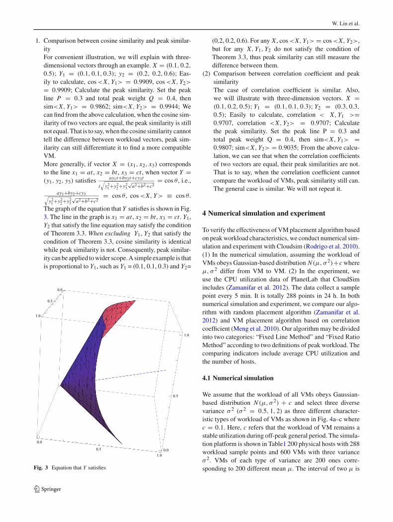
The graph of the equation that Y satisfies is shown in Fig.3. The line in the graph is x1 = at , x2 = bt , x3 = ct . Y1,Y2 that satisfy the line equation may satisfy the conditionof Theorem 3.3. When excluding Y1, Y2 that satisfy thecondition of Theorem 3.3, cosine similarity is identicalwhile peak similarity is not. Consequently, peak similar-ity canbe applied towider scope.A simple example is thatis proportional to Y1, such as Y1 = (0.1, 0.1, 0.3) and Y2=

0.0

0.5

1.0

0.0

0.51.0

0.0

0.5

1.0

Fig. 3 Equation that Y satisfies

(0.2, 0.2, 0.6). For any X , cos<X,Y1> = cos<X, Y2>,but for any X,Y1,Y2 do not satisfy the condition ofTheorem 3.3, thus peak similarity can still measure thedifference between them.

(2) Comparison between correlation coefficient and peaksimilarityThe case of correlation coefficient is similar. Also,we will illustrate with three-dimension vectors. X =(0.1, 0.2, 0.5); Y1 = (0.1, 0.1, 0.3); Y2 = (0.3, 0.3,0.5); Easily to calculate, correlation < X,Y1 >=0.9707, correlation <X,Y2> = 0.9707; Calculatethe peak similarity. Set the peak line P = 0.3 andtotal peak weight Q = 0.4, then sim<X, Y1> =0.9807; sim<X,Y2> = 0.9035; From the above calcu-lation, we can see that when the correlation coefficientsof two vectors are equal, their peak similarities are not.That is to say, when the correlation coefficient cannotcompare the workload of VMs, peak similarity still can.The general case is similar. We will not repeat it.

4 Numerical simulation and experiment

To verify the effectiveness of VMplacement algorithm basedon peakworkload characteristics, we conduct numerical sim-ulation and experiment with Cloudsim (Rodrigo et al. 2010).(1) In the numerical simulation, assuming the workload ofVMs obeys Gaussian-based distribution N (μ, σ 2)+cwhereμ, σ 2 differ from VM to VM. (2) In the experiment, weuse the CPU utilization data of PlanetLab that CloudSimincludes (Zamanifar et al. 2012). The data collect a samplepoint every 5 min. It is totally 288 points in 24 h. In bothnumerical simulation and experiment, we compare our algo-rithm with random placement algorithm (Zamanifar et al.2012) and VM placement algorithm based on correlationcoefficient (Meng et al. 2010). Our algorithmmay be dividedinto two categories: “Fixed Line Method” and “Fixed RatioMethod” according to two definitions of peak workload. Thecomparing indicators include average CPU utilization andthe number of hosts.

4.1 Numerical simulation

We assume that the workload of all VMs obeys Gaussian-based distribution N (μ, σ 2) + c and select three diversevariance σ 2 (σ 2 = 0.5, 1, 2) as three different character-istic types of workload of VMs as shown in Fig. 4a–c wherec = 0.1. Here, c refers that the workload of VM remains astable utilization during off-peak general period. The simula-tion platform is shown in Table1 200 physical hosts with 288workload sample points and 600 VMs with three varianceσ 2. VMs of each type of variance are 200 ones corre-sponding to 200 different mean μ. The interval of two μ is

123

Design and theoretical analysis of virtual machine placement algorithm based on peak workload. . .

(a)

(b)

(c)

Fig. 4 Image of VMs’ workload

28.8/200=0.144. μn = 0.144n − 0.072, n = 1, 2, . . . , 288.

The workload has the form: fn(t) = 1σ√2π

e− (t−μn )2

2σ2 + c,t ∈ [0, 28.8]. c takes 0.1 in the simulation. We compare ouralgorithm with random placement algorithm and VM place-ment algorithm based on correlation coefficient.

The three images are more and more “gentle”, more andmore “dispersed” as σ 2 grows. The image of σ 2 = 0.5 isconcentrated with the maximum reaching more than 0.65

Table 1 Experiment platform

Experiment parameter Value

Number of physical hosts 200

Number of VMs 600

Total peak weight Q 0.4

Fig. 5 Average utilization of numerical simulation

and the peak is mainly distributed in the range of [13, 16].The image of σ 2 = 2 is slightly gentle with large peak spanranging mainly in (Kim et al. 2013; Chen et al. 2014) andthus the maximum is less than 0.4. The image of σ 2 = 1 isin between them. Three images show three types of differentworkload characteristics. Some show the characteristic thattheir peaks gently occur. Some reach their peaks in a shorttime. Combination of various types of VMs may see a hugedifference regarding consolidation.

The numerical simulation results is shown in Figs. 5 and6. The utilization of random placement algorithm in Figs. 5and 6 is the average of 10 results. From Fig. 5, we can see thatboth fixed linemethod and fixed ratiomethod aremuch bettercompared with the random method and correlation coeffi-cient method. Fixed peakmethod achieves 15.55% improve-ments compared with random method and 8.84% comparedwith correlation coefficient method in terms of the averageutilization. Likewise, comparing results of fixed ratiomethodof that is 13.24 and6.53%.Figure 6 shows the number of usedhosts. In comparison with randommethod, fixed line methodreduces 33.7 hosts, 22.5%savings. In comparisonwith corre-lation coefficientmethod, it is 17 hosts, 12.8% savings. Fixedratio method achieves a reduction of 29.7 hosts, 19.8% sav-ings in comparison with random method and 13 hosts, 9.8%savings in comparison with correlation coefficient method.

The results of numerical simulation illustrate that withregard to the VMs whose workload obeys Gaussian-baseddistribution N (μ, σ 2) + c, our VM placement algorithmbased on peak similarity could consolidate VMs moreeffectively in light of the peak workload characteristic. It sig-

123

W. Lin et al.

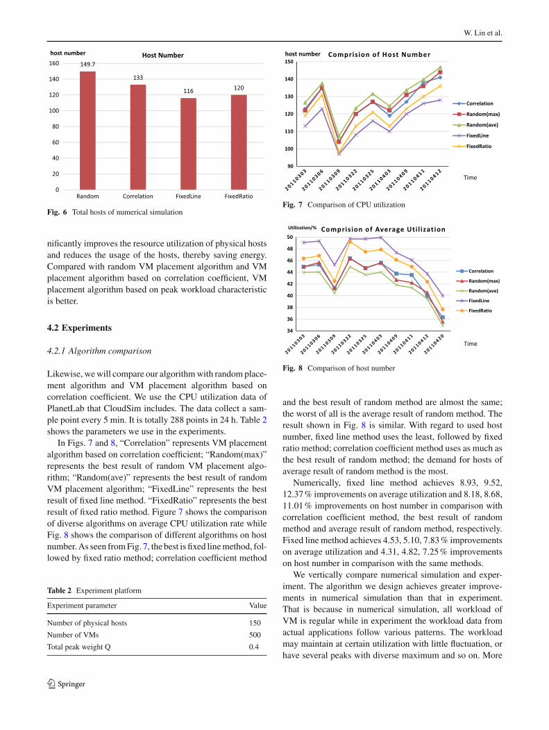
Fig. 6 Total hosts of numerical simulation

nificantly improves the resource utilization of physical hostsand reduces the usage of the hosts, thereby saving energy.Compared with random VM placement algorithm and VMplacement algorithm based on correlation coefficient, VMplacement algorithm based on peak workload characteristicis better.

4.2 Experiments

4.2.1 Algorithm comparison

Likewise, wewill compare our algorithmwith random place-ment algorithm and VM placement algorithm based oncorrelation coefficient. We use the CPU utilization data ofPlanetLab that CloudSim includes. The data collect a sam-ple point every 5 min. It is totally 288 points in 24 h. Table 2shows the parameters we use in the experiments.

In Figs. 7 and 8, “Correlation” represents VM placementalgorithm based on correlation coefficient; “Random(max)”represents the best result of random VM placement algo-rithm; “Random(ave)” represents the best result of randomVM placement algorithm; “FixedLine” represents the bestresult of fixed line method. “FixedRatio” represents the bestresult of fixed ratio method. Figure 7 shows the comparisonof diverse algorithms on average CPU utilization rate whileFig. 8 shows the comparison of different algorithms on hostnumber.As seen fromFig. 7, the best is fixed linemethod, fol-lowed by fixed ratio method; correlation coefficient method

Table 2 Experiment platform

Experiment parameter Value

Number of physical hosts 150

Number of VMs 500

Total peak weight Q 0.4

Fig. 7 Comparison of CPU utilization

Fig. 8 Comparison of host number

and the best result of random method are almost the same;the worst of all is the average result of random method. Theresult shown in Fig. 8 is similar. With regard to used hostnumber, fixed line method uses the least, followed by fixedratio method; correlation coefficient method uses as much asthe best result of random method; the demand for hosts ofaverage result of random method is the most.

Numerically, fixed line method achieves 8.93, 9.52,12.37% improvements on average utilization and 8.18, 8.68,11.01% improvements on host number in comparison withcorrelation coefficient method, the best result of randommethod and average result of random method, respectively.Fixed line method achieves 4.53, 5.10, 7.83% improvementson average utilization and 4.31, 4.82, 7.25% improvementson host number in comparison with the same methods.

We vertically compare numerical simulation and exper-iment. The algorithm we design achieves greater improve-ments in numerical simulation than that in experiment.That is because in numerical simulation, all workload ofVM is regular while in experiment the workload data fromactual applications follow various patterns. The workloadmay maintain at certain utilization with little fluctuation, orhave several peaks with diverse maximum and so on. More

123

Design and theoretical analysis of virtual machine placement algorithm based on peak workload. . .

Fig. 9 Comparison of execution time

importantly, parameter c in numerical simulation takes 0.1,meaning that application stays at a small utilization in the off-peak period, which may be too small in comparison with theactual situation. Therefore, the simulation results are moreclose to the reality.

4.2.2 Comparison of execution time

Next, we will compare the execution time of the abovealgorithms. Algorithm complexity of these four methods isO(mn2) where m is the dimension of workload vector andn is the number of VMs. The workload data collect a sam-ple point every 5min. It is totally 288 points in 24 h. Thus,m = 288. n takes 100, 200 as sample. Each algorithm runs20 times and Fig. 9 shows the average execution time.

Figure 9 illustrates random method runs fastest becauseof its small amount of computation. The speed of fixed linemethod and correlation coefficientmethod is nearly the same.Fixed ratiomethod is slowest and the speed gapwith the otherthree is wide because when calculating weights fixed ratiomethod iterates through the workload data to calculate themean, bringing about more calculations. However, in view ofthe actual experimental results, the algorithm execution timeof 200 VMs is merely about 3 s (3092 ms). It is acceptablefor VM placement in cloud computing center.

5 Conclusion and future work

Based on the basic idea of resource multiplying, this paperaims to consolidateVMswith differentworkload characteris-tics, and improve resource utilization. Throughmathematicalmodeling, we define a new mathematical quantity-peak sim-ilarity to measure the similarity of VMs’ peak workload.The effectiveness is proved from the perspective of theo-retical analysis, numerical simulation and the algorithmsexperiments. Theoretical proof gives necessary and suffi-cient conditionswhen the peak similarity is identical, therebyyielding peak similarity has a broader scope than cosine

similarity and correlation coefficient. Application of peaksimilarity is not limited to VM placement. It is a generalmathematical quantity that can be applied to other resourcecomplementary scenes. Hence, this paper is an applicationexample of peak similarity. Numerical simulation shows thatwith regard to the VMs whose workload obeys Gaussian-based distribution , our VM placement algorithm is betterthan random VM placement algorithm and VM placementalgorithm based on correlation coefficient. Employing actualworkload data, the experiments validate the effectiveness ofour proposed VM placement algorithm more accurately.

At present, the proposed VM placement algorithm basedon peak workload characteristics only considers constraintsof CPU resource without considering memory, bandwidthand other resources. Often, VMs demand for one resourcea lot but little for others. For the problem of multi-dimensional resource constraints, peak similarity may beapplied to describe the similarity of VMs’ demands forvarious resources as well. For instance considering threeresources: CPU, ram and IO, we could calculate their threepeak similarities respectively. These three peak similaritiesshould be smaller than a certain threshold value and then sortthe VMs according to the sum of three peak similarities toselect the suitable VM for consolidation. Specific implemen-tation will be the direction of future research.

Acknowledgments Thisworkwaspartially supportedby theNationalNatural Science Foundation of China (Grant Nos. 61402183, 61272382and 61202466), Guangdong Natural Science Foundation (Grant No.S2012030006242), Guangdong Provincial Science and technologyprojects (Grant Nos. 2013B010401024, 2013B010401005, 2013B090200021, 2014B010117001, 2014A010103022 and 2014A010103008),and Guangzhou Science and Technology Fund of China (GrantNos. 2012J4300038, LCY201206, 2013J4300061 and 2013Y200077),and Fundamental Research Funds for the Central Universities (Nos.2014ZM0032 and 2015ZZ0038).

Compliance with ethical standards

Conflicts of interest The authors declare that they have no conflict ofinterest.

References

Agrawal S, Bose SK, Sundarrajan S (2009) Grouping genetic algorithmfor solving the server consolidation problem with conflicts. In:Proceedings of the first ACM/SIGEVO summit on genetic andevolutionary computation. ACM, pp 1–8

Calheiros NR, Rajiv R et al (2011) CloudSim: a toolkit for modelingand simulation of cloud computing environments and evaluationof resource provisioning algorithms. Softw Pract Exp 41(1):23–50

Chen R, Qi D, Lin W, Li J (2014) An integrated scheduling algorithmfor virtual machine system on asymmetric multi-core processors.Chin J Comput 37(7):1466–1477

ChenM,ZhangH, SuYYet al (2011) EffectiveVMsizing in virtualizeddata centers. In: Proceedings of integrated network management(IM), 2011 IFIP/IEEE international symposium on. IEEE, pp 594–601

123

W. Lin et al.

Chen K, Zheng W (2009) Cloud computing: system instances and cur-rent research. J Softw 20(5):1337–1348

Dong J, Wang H, Li Y, Cheng S (2014) Improving energy efficiencyandnetwork performance in IaaS cloudwith virtualmachine place-ment. J Commun 35(1):72–81

Foster I, Zhao Y, Raicu I, Lu S (2008) Cloud computing and gridcomputing 360-degree compared, GCE ’08 grid computing envi-ronments workshop, pp 1–10

Gao Y, Guan H, Qi Z et al (2013) A multi-objective ant colony systemalgorithm for virtual machine placement in cloud computing. JComput Syst Sci 79(8):1230–1242

Hirofuchi T, Nakada H, Ogawa H et al (2010) Eliminating datacenteridle power with dynamic and intelligent vm relocation. Distributedcomputing and artificial intelligence. Springer, Berlin, pp 645–648

Hu J, Gu J, Sun G (2010) A scheduling strategy on load balancingof virtual machine resources in cloud computing environment. In:Parallel architectures, algorithms and programming (PAAP), 2010third international symposiumon. IEEE, pp 89–96

Kim J, Ruggiero M, Atienza D, et al (2013) Correlation-aware virtualmachine allocation for energy-efficient datacenters. In: Proceed-ings of the conference on design, automation and test in Europe.EDA consortium, pp 1345–1350

Li M, Bi J, Li Z (2014) Resource-scheduling-waiting-aware virtualmachine consolidation. J Softw 25(7):1388–1402

Lin W, Wang JZ, Liang C, Qi D (2011) A threshold-based dynamicresource allocation scheme for cloud computing. ProcEng23:695–703

LinW, Liu B, Zhu L, Qi D (2013) CSP-based resource allocation modeland algorithms for energy-efficient cloud computing. J Commun12:33–41

Lin W, Zhu C, Li J et al (2015) Novel algorithms and equivalenceoptimisation for resource allocation in cloud computing. Int JWebGrid Serv 11(2):193–210

Lin W, Qi D (2012) Survey of resource scheduling in cloud computing.Comput Sci 39(10):1–6

Liu Z, Wang S, Sun Q, Yang F (2012) Energy-aware intelligent opti-mization algorithm for virtual machine replacement. J HuazhongUniv Sci Technol (Nat Sci Edn) 40(S1):398–402

Meng X, Isci C, Kephart J et al (2010) Efficient resource provisioningin compute clouds via vm multiplexing. In: Proceedings of the7th international conference on autonomic computing. ACM, pp11–20

Nakada H, Hirofuchi T (2009) Toward virtual machine packing opti-mization based on genetic algorithm.LNCS 5518:Berlin, Heidel-berg: proceedings of the 10th international work conference onartificial neural networks: part 2: distributed computing, artificialintelligence bioinformatics soft computing and ambient assistedliving, pp 651–654

Wang X, Wang Y, Cui Y (2014) An energy-aware bi-level optimizationmodel for multi-job scheduling problems under cloud computing.Soft Comput. doi:10.1007/s00500-014-1506-3

Wei L, Huang T, Chen J, Liu Y (2013) Workload prediction-basedalgorithm for consolidation of virtual machines. J Electron InfTechnol 35(6):1271–1276

Xu B, Peng Z, Xiao F et al (2014) Dynamic deployment of virtualmachines in cloud computing using multi-objective optimization.Soft Comput 19(8):2265–2273

Zamanifar K, Nasri N, Nadimi-Shahraki M (2012) Data-aware virtualmachine placement and rate allocation in cloud environment. In:Proceedings of 2012 second international conference on advancedcomputing and communication technologies (ACCT). IEEE, pp357–360

123