design and test of low-profile composite aerospace tank dome€¦ · design and test of low-profile...

NASA/TP--1999-209267

Design and Test of Low-Profile Composite

Aerospace Tank Dome(MSFC Center Director's Discretionary Fund Final Report,

Project No. 96-28)

R. Ahmed

Marshall Space Flight Center, Marshall Space Flight Center, Alabama

National Aeronautics and

Space Administration

Marshall Space Flight Center • MSFC, Alabama 35812

May 1999

https://ntrs.nasa.gov/search.jsp?R=19990046771 2020-05-13T02:12:07+00:00Z

Acknowledgments

The author gratefully acknowledges the efforts of the following people in the completion of this task:

• Derek Gefroh of University of Minnesota, NASA Academy Summer Student

• Robert Huff, Larry Pelham, and Gary Smith of Thiokol Corporation

• Marc Verhage, Steve Miller, and Chuck Wilkerson of NASA/MSFC.

A great many other people, whose names could not all be recalled by the author, worked to make this

project a success. The author gratefully acknowledges their participation as well.

Available from:

NASA Center for AeroSpace Information

800 Elkridge Landing RoadLinthicum Heights, MD 21090-2934

(301 ) 621-0390

National Technical Information Service

5285 Port Royal Road

Springfield, VA 22161(703) 487-4650

ii

TABLE OF CONTENTS

I. INTRODUCTION .....................................................................................................................

1A. Purpose .................................................................................................................................

B. Summary ............................................................................................................................... 1

LOW-PROFILE COMPOSITE DOME DESIGN AND MANUFACTURE ................................ 2

A. Design Principles for Low-Profile Composite Domes ......................................................... 2

B. Application to Composites ................................................................................................... 7

C. Design Derivation ................................................................................................................. 9

D. Manufacturing ...................................................................................................................... 10

12III. ANALYSIS ................................................................................................................................

A. Analytical Solutions ............................................................................................................. 12B. Finite Element Solutions ...................................................................................................... 37

39IV. TEST ..........................................................................................................................................

A. Test Article ............................................................................................................................ 39

B. Test Fixture Description ....................................................................................................... 39

C. Test Setup and Pressure Loading .......................................................................................... 39

D. Instrumentation ..................................................................................................................... 40

E. Test Procedure ...................................................................................................................... 4141E Results ..................................................................................................................................

V. DISCUSSION ............................................................................................................................ 42

A. Ultimate Failure .................................................................................................................... 42

B. Displacement and Strain Versus Pressure ............................................................................. 43

VI. CONCLUSION .......................................................................................................................... 45

REFERENCES .................................................................................................................................... 46

II.

.,°

111

LIST OF FIGURES

.

_°

3.

4.

5.

,

7.

8.

9.

10.

11.

12.

13.

14.

15.

16.

17.

18.

19.

20.

Stresses on a differential element in a generic shell of revolution .......................................

Definition of normals for calculating stress field in elliptical shell .....................................

Completed low-profile composite dome ..............................................................................

Interface ring used to secure dome to base plate ..................................................................

Predicted and actual meridional strains versus pressure, gauge 1MB 1................................

Predicted and actual circumferential strains versus pressure, gauge 2MB 1.........................

Predicted and actual meridional strains versus pressure, gauge 1MB2 ................................

Predicted and actual circumferential strains versus pressure, gauge 2MB2 .........................





Predicted and actual meridional stratus versus pressure, gauge 1MB5 ................................

Predicted and actual circumferential stratus versus pressure, gauge 2MB5 .........................



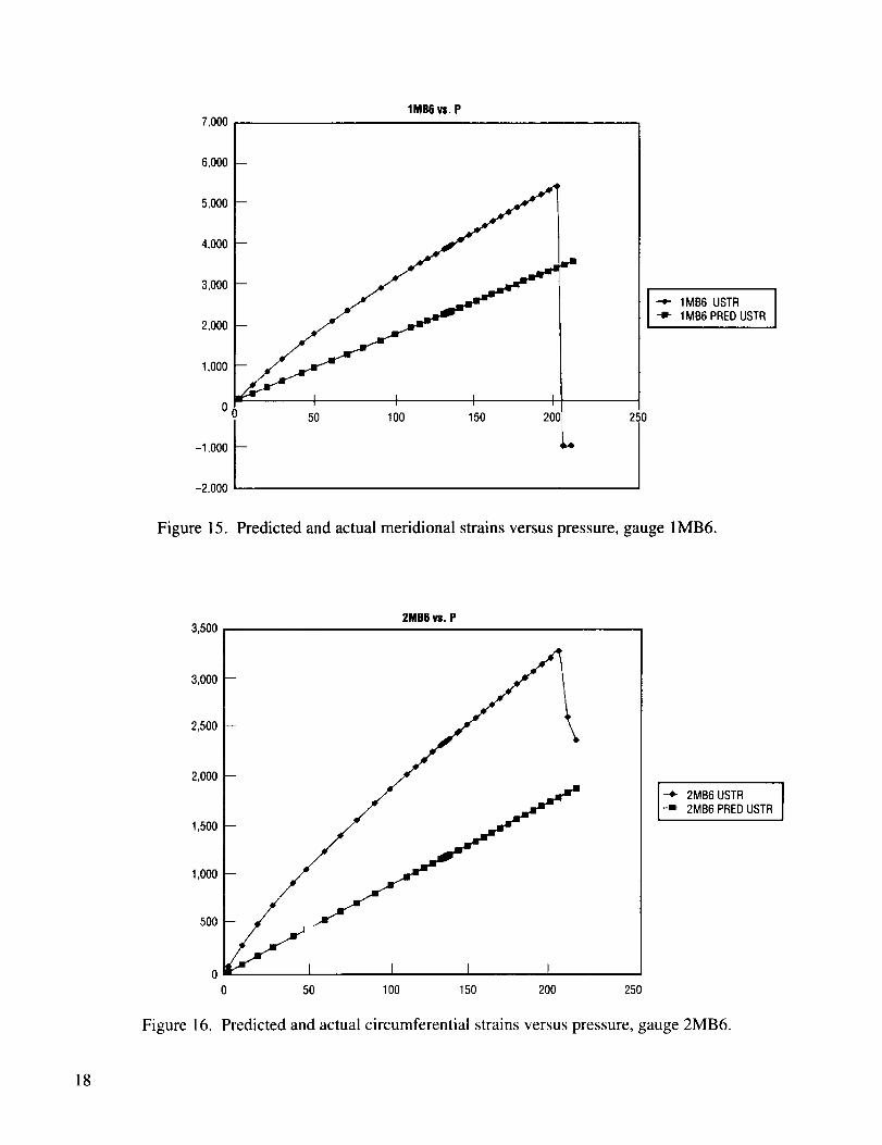
Predicted and actual meridionai strains versus pressure, gauge 1MB7 ................................


Predicted and actual meridional strains versus pressure, gauge I MB8 ................................


3

5

11

11

13

13

14

14

15

15

16

16

17

17

18

18

19

19

20

20

iv

LIST OF FIGURES (Continued)

21.

22.

23.

24.

25.

26.

27.

28.

29.

30.

31.

32.

33.

34.

35.

36.

37.

38.

39.

40.

41.

Predicted and actual meridional stratus versus pressure, gauge 1MB9 ................................


Predicted and actual meridional stratus versus pressure, gauge 1MB 10 ..............................

Predicted and actual circumferential stratus versus pressure, gauge 2MB 10 .......................





Predicted and actual meridional strasns versus pressure, gauge I MB 13 ..............................




Predicted and actual meridional strains versus pressure, gauge 1MB 15 ..............................


Predicted and actual meridional stratus versus pressure, gauge 1MB16 ..............................


Predicted and actual displacements versus pressure, gauges DH 1, DV1 .............................

Predicted and actual displacements versus pressure, gauges DH2, DV2 .............................




21

21

22

22

23

23

24

24

25

25

26

26

27

27

28

28

29

29

30

30

31

V

LIST OF FIGURES (Continued)

42.

43.

44.

45.

46.

47.

48.

49.

50.

51.

52.

53.

54.

55.

56.

57.

58.





Predicted and actual displacements versus pressure, gauges DH 10, DVI0 .........................

Predicted and actual displacements versus pressure, gauges DH11, DV11 .........................

Predicted and actual displacements versus pressure, gauges DH 12, DV 12 .........................



Predicted and actual displacements versus pressure, gauges DHI5, DVI5 .........................

Predicted and actual displacements versus pressure, gauges DH16, DVI 6 .........................

Finite element mesh of low-profile composite dome ...........................................................

First mode buckling of low-profile composite dome ...........................................................

Test setup ..............................................................................................................................

Strain gauge layout ...............................................................................................................

Low-profile composite dome after failure ............................................................................

Closeup of one of the failure regions on low-profile composite dome ................................

31

32

32

33

33

34

34

35

35

36

36

37

38

40

40

42

58

vi

LIST OF TABLES

°

2.

Layup and loads of low-profile composite dome as a function of position .........................

Material properties of IM7/8552 graphite composite cloth material ....................................

8

12

vii

TECHNICAL PUBLICATION

DESIGN AND TEST OF LOW-PROFILE COMPOSITE AEROSPACE TANK DOME

(MSFC Center Director's Discretionary Fund Final Report, Project No. 96-28)

I. INTRODUCTION

In order to increase the structural performance of cryogenic tanks, the aerospace industry has begun

to employ low-profile bulkheads in launch vehicle designs. A low-profile dome has a major-to-minor axis

ratio greater than the square root of 2 and offers possibilities for maximizing the volume of a tank for a

given length or for a shorter overall vehicle length for a given propellant volume. It can also minimize the

length of interstage segments that join tanks together, thus contributing to a lower overall vehicle weight.

Previous studies have examined metallic aluminum alloy low-profile domes, but at the time of this

writing limited work has been performed on low-profile domes constructed from composite materials.

Composite materials offer the potential for further weight reduction over metallic materials due to the

former's directional properties and higher strength-to-weight ratios. Consequently, a test project was initiated

under the auspices of the Center Director's Discretionary Fund at the NASA Marshall Space Flight Center

(MSFC) to validate the low-profile dome concept using a commonly used advanced aerospace composite

material in a subscale (_1 m diameter) low-profile dome. This report describes the design, analysis, test,

and results of this dome project.

A. Purpose

The objectives of the low-profile composite dome test were as follows:

I. Demonstrate the feasibility of low-profile composite dome designs.

2. Examine the structural response and failure modes for internally pressurized low-profile composite

domes as a function of ply layup, number of plies (thickness), and a given fiber/matrix combination. The

dome was appropriately instrumented to measure strain, displacement, and pressure under the applied

loads. The data obtained from these tests would then be compared to analysis models and design guidelines

for low-profile composite domes suggested.

B. Summary

This report presents the methodology behind the design of the low-profile composite dome, the

means of its manufacture, the structural analysis that went into verifying the design before test, and the test

itself. Test results (strains and displacements) are compared to the analysis predictions. Finally, assessments

of the test article's strength and failure modes are given, along with suggestions for design of a low-profile

composite dome.

II. LOW-PROFILE COMPOSITE DOME DESIGN AND MANUFACTURE

The low-profile composite dome was designed and manufactured during the spring and summer of

1996 (February through August) with the assistance of the Thiokol Corporation and the MSFC Productivity

Enhancement Complex (PEC).

A. Design Principles for Low-Profile Composite Domes

To design a low-profile dome, it is necessary to have an understanding of the stress fields that occur

in a vessel of revolution, which is created by rotating a two-dimensional shape about an axis through 360 °.

The membrane stresses in such a vessel of revolution are axisymmetric; i.e., they are the same in any plane

perpendicular to the axis of rotation. Figure 1 shows a generic shell of revolution and the stresses on a

differential element. Only normal stresses act on this element.

The quantities in figure 1 are defined as follows:

al = stress in meridional direction

0-2 = stress in hoop direction (direction along shell in circle perpendicular to axis of revolution)

rl = radius of curvature of element in meridional direction at a point

r2 = radius of curvature of element in hoop direction at a point

ds! = element arc length in meridional direction

ds 2 = element arc length in hoop direction

dO l = angle swept by arc length in meridional direction

dO 2 = angle swept by arc length in hoop direction

h = thickness of shell

p = pressure applied (positive for internal pressure).

Applying equilibrium to the element in figure 1 gives:

2G2hdsl sin + 2_lhds 2 sln_-_---)= P(rlsindOlr2sind02) . (1)

2

0

(a)

F

,,,

,j\/{el

Figure 1. Stresses on a differential element in a generic shell of revolution.

Substituting ds 1 = rldO 1 and ds 2 = r2dO 2 into (1) and noting that sin dO = 0 for small angles yields

the following:

a2hr 1 + crlhr2 = prlr 2 (2)

Rearranging (2) gives us:

_2 _Crl=plh (3)r2 rl

It is important to note again that r I is the local radius of curvature in the meridional direction, while

r 2 is the radius of curvature in the hoop direction normal to the surface of the ellipsoid at a given point, r 1

is found using the curvature relation from elementary calculus and the equation of an ellipse as follows:

l+y,2] /2r I =t9 = , (4)

and

x 2 y2

a 2 + _- = 1 , (5)

where y' is the first derivative ofy with respect to x, y" is the second derivative ofy with respect to x, and a

and b are the major and minor axes, respectively, of the ellipse.

Rearranging (5) gives:

(6)

Finding y' and y" from (6) yields:

b x 2

V'= a [a 2_ 112 = - x- y

(7)

b 4

y- = _ a2y3(8)

Substituting (7) and (8) into (4) brings forth the following expression:

a4y2+b4x213/2

rI = a4b4(9)

To find r 2, the normal to the surface is used as shown in figure 2. Defining I as the vertical compo-

nent of r2:

r2= [12+x2] 1/2 (lO)

4

Figure2.

0I

Y

" - I, Axis0f Rotation

YX

Definition of normals for calculating stress field in elliptical shell.

Noting that tanO = x / l = y' yields the following:

with

l=X=

y'

Substituting (7) and (12) into (11):

r 2 =[12(1+y'2)] 1/2

a2y

7_-= (b)_a2 - x2] 1/2

(11)

(12)

b 2

Taking the ratio of r 1 and r2 gives:

(13)

/bj)rl = r2 3(14)

5

Now,applyingequilibriumequationsto acut asshownin figure2:

with

p_rx2 _ crI (2 n:x)h sin 0 = 0 (15)

X

sin 0 = r2(16)

Substituting (16) into (15) and rearranging gives:

pr2

crl= 2h (17)

Substituting (17) into (3):

0"2 = 2h _ q ' (18)

remembering that (71 is the meridional stress and cr2 is the hoop stress.

A summary of the key equations for computing stresses in low-profile domes follows:

Equation (6)

Equation (9)a4y +b4x 2 ]3/2

r I = a4b4

Equation (13)

Equation (14)

a4y2+x2b4] /2

r 2 = b2

rl = r2 3

pr2Equation (17) crl = 2--h-

Pr2/2- /Equation (18) 0"2 = 2h _ _ "

Note that these equations are valid for computing overall average stresses through the thickness of

the membrane regardless of the material properties.

Equation (18) shows that compressive hoop stresses will appear at equatorial locations in domes

with r 1 > 2r2. Of particular interest is the a/b ratio required to keep all hoop stresses greater than zero.

Looking at an ellipse, one can visualize that r 1 increases dramatically and r 2 increases only slightly as one

moves from the equator toward the apex. This means that the minimum hoop stress is at the equator as seen

from equation (18). To find the a/b ratio for a zero hoop stress at the equator, equation (9) is substituted

into equation (18) while setting x = a and y = 0 (the location of the dome equator). This yields a/b = \/2.

Low-profile domes are those that have an a/b ratio > v_. By substituting appropriate values of a and b into

equation (9) such that a/b>_/2and setting x=a andy=0, one can use equations (13) and (18) to show that

the hoop stresses are negative (compressive) at the dome equator.

Equatorial buckling becomes a concern in low-profile domes that have high compressive hoop

stresses.

High-strength composites have the capability, when appropriately oriented, to handle the high prin-

cipal stresses encountered at the apexes of a low-profile dome as well as the high compressive stresses near

the dome equator. It is therefore feasible to design a composite dome of varying thicknesses and layup

angles to meet the different stress states at different meridional locations.

B. Application to Composites

To design a low-profile dome using composite materials, it is useful to look at the hoop and meridi-

onal line loads (which are equal to the corresponding stress multiplied by the thickness). This is very

helpful in design since thicknesses are initially unknown and must be selected. Using the equations derived

above, a table of hoop and meridional load versus coordinate location on the dome can be derived. This is

shown in table 1 for the tested dome, which had an equatorial diameter of 40.2 in. and a 3-to-1 radius-to-

height ratio.

After having mapped the line loads as a function of position on the dome, the various stress states

and potential failure modes must be considered. Several potential failure modes are possible in a low-

profile dome: biaxial tension, biaxial tension-compression (shear), and hoop compression buckling. Since

the dome was constructed by hand layup of individual gore sections, the resulting seams weaken the design

and must be compensated for to prevent premature failure. Test hardware and support equipment also

influenced the dome's design; potential shearout at the bolted joint interface between the dome and the

supporting base plate was a major concern.

7

o_

o

o.B

n_

"s

E

o0

on3

c6

ot_

o_J

comv

CO CO cO O_ r_ r_ O_ ,_ ._ _ O_ eo c,_ _ O_ _o o uo co o_ o o co co c_

0

e_i

o

,m

ooo E

o

. co

©

©

..o

E¢o

#

0Bv

C. Design Derivation

The dome was designed using composite laminate theory to meet a 100 psi internal pressure limit

load. The line loads were input into the equations for a laminate to derive the stresses and strains of the

laminate by using a weighted average of all the lamina stiffnesses in a given direction in the laminate. The

total strain through the thickness was assumed constant. In addition, the laminate was assumed to be stacked

in a manner symmetric about its centerline. This was not the case in the actual hardware, although the

majority of the plies were of 0 ° and 90 ° orientations, whose stiffness and strength properties were similar

to each other. At 100 psi pressure, the ply layups were chosen to give a safety factor of at least 2.0 on first

ply failure (FPF) based on the biaxial tension or biaxial tension-compression with the Tsai-Hill failure

criterion. This was the case because other failure modes (failure at seams, buckling) were thought to occur

well before twice the limit load. The goal was to ensure that the dome would meet an ultimate safety factor

of 1.4 against these other modes.

To determine the actual ply layups, a FORTRAN computer code was written to calculate lamina

stresses and strains based on the stated assumptions of constant strain through the shell thickness. A spread-

sheet calculating the loads and overall stresses in the hoop and meridional directions as a function of dome

position was prepared using the analytical equations described earlier in this report. These line loads were

used as inputs into the FORTRAN program to generate the required layup to meet the safety factor of 2.0

on FPE This was accomplished via a "cut and try" method of selecting a layup combination, running the

FORTRAN program to determine if it met the safety factor, and then modifying the layup as necessary

until a suitable combination was found. This procedure was repeated at various locations along the dome

meridian from equator to apex such that a structurally acceptable layup profile was developed. The layup

as a function of dome coordinate position is shown in table 1.

After a basic layup profile was found, design details could then be examined. One of these was the

interface of the dome to the associated test fixture hardware, an arrangement which consisted of 75 9/16-in.

diameter bolts. The resulting joint subjects the bolts to shear loads and the composite material around the

bolt holes to bearing, tearout, and shearout loads. This joint was designed using a computer program

known as the Bolted Joint Stress Field Model (BJSFM). 2 This software allows a designer to input ply

orientations, thicknesses, loads, etc. and calculate the failure load of the joint. Using this tool, a layup

arrangement using 0 °, 90 °, 45 °, and -45 ° plies was devised. This ensured that this joint would fail at 339

psi, far above the expected dome failure loads in the 150- to 200-psi range.

As is explained in the next section, the dome was manufactured by hand from layers of precut gores

in order to give the dome the correct shape when laid up on the mandrel. Such methods introduce seams in

the finished product that run along the meridional direction from apex to equator. The resulting stress

concentrations and shear concentrations were taken into account via a simple finite element analysis, which

predicted failure stresses would be reached in the 150-psi range of internal pressure.

Additional analyses and design exercises were required to ensure no leaks would result during the

test, to determine bolt torquing requirements, and to ensure structural integrity of the aluminum base plate

and cover plate structures that were used in the test.

D. Manufacturing

The low-profile composite dome was manufactured using precut gore sections of IM7/8552 cloth

graphite-epoxy material laid up by hand on a steel mandrel. This method, while labor-intensive, ensured

that the dome would have adequate strength in both the hoop and meridional directions and allowed the

number of layers and the resulting dome thickness to be easily varied as a function of stress state along the

dome meridian. In effect, it allowed the dome to be design optimized; this would have been very difficult,

to impossible, to accomplish using the state-of-the-art filament-winding or fiber-placement techniques of

the time with their unidirectional tape arrangements. Tailoring the thicknesses of unidirectional tape to

meet the stress state and even winding it in such a way as to resist the highly varying stress states encoun-

tered in a low-profile dome was, at the time, a very formidable task and would have resulted in a much

heavier and thicker dome than resulted from the hand layup with the IM7/8552 cloth material and its highly

bidirectional stiffness and strength properties.

The following procedure was used to manufacture the dome:

1. Gores (each sweeping 22.5 °) were precut with proper orientations (0 °, 900,45 °, and -45 °) to the

required lengths and widths for layup on the mandrel.

2. Sixteen full-length gores were laid on the mandrel to form the first layer of the dome, followed

by subsequent layers offset 1 to 2 in., circumferentially. This was done to prevent continuous seams through

the entire thickness or a large part of the thickness. Subsequent shorter gores were used to make the buildup

areas near the equator and apex regions of the dome.

3. Debulking was performed periodically during the layup process to ensure that gores remained

positionally stable and remove air bubbles. A vacuum bag was attached to the entire layup and evacuated,

allowing atmospheric pressure to compress the layup against the mandrel.

4. After all gores were laid and a final debulk was performed, the dome was vacuum-bagged and

autoclaved for more than 8 hr at 300 °F and a pressure higher than atmospheric.

5. A 4-in. diameter hole was drilled into the apex of the dome to accommodate the cover plate

(which held the overflow and relief valves used in the test). Sixteen bolt holes for securing the cover plate

were drilled around this large hole. The bottom of the dome below the equator was final-machined to bring

the total dome height to 10.015 in. Seventy-five bolt holes for securing the equator to the base plate inter-

lace ring were also drilled.

The finished dome is shown in figure 3. The final dimensions of the dome were 40.2 in. in diameter

and 10.015 in. in height (in final-machined configuration). The weight of the dome without the interface

ring and the cover plate was approximately 11 lb. The interface ring used to bolt the dome to the base plate

is shown in figure 4.

10

Figure3. Completedlow-profile compositedome.

Figure4. Interfacering usedto securedometo baseplate.

11

III. ANALYSIS

Both analytical analysis and finite element methods were used to calculate predicted stresses,

strains, displacements, and failure loads. Failure can occur in one or all of the following ways: circum-

ferential hoop buckling, biaxial tension, and biaxial tension-compression (shear). As shown earlier, the

stress state as a function of position on the dome was known analytically via the dome stress equations.

Beginning with the known stress state, composite laminate theory was used to calculate the resulting

strains and stresses in the material directions of the individual layers. These were then used to estimate

the expected failure loads via the Tsai-Hill failure criterion.

A. Analytical Solutions

Since the overall stress state was known, finite element analysis was not necessary to determine

the stresses and strains at a given point in the dome. These were determined using established methods

of composite laminate theory treated by Tsai and Hahn 3 and other authors. The detailed methods are

described in their books and only an outline of the procedure is given here. It should be noted at this

point that only in-plane stiffness analysis was used here, which meant that any asymmetry in the layups

was ignored. This was done because the stiffness and strength properties of the IM7/8552 cloth material

were similar in their orthogonal directions and, therefore, asymmetry was not considered to affect the

resulting solutions. Time and manpower constraints prevented the more detailed approach of evaluating

the in-plane/bending moment coupled stiffnesses and the bending stiffnesses. The same FORTRAN

program used to derive the layup was also used to determine the on-axis ply stresses and strains given

the stress state known via the dome stress equations in the circumferential-meridional dome coordinate

system.

The material properties of the IM7/8552 cloth material are shown in table 2. The warp and fill

stiffnesses were both approximately 12 msi and their strengths approximately 125 to 130 ksi in the

orthogonal directions. The test strain and displacement predictions are shown with their corresponding

actual gauge readings in figures 5 through 52.

Table 2. Material properties of IM7/8552 graphite composite cloth material.

MaterialPropertiesForIM7/8552Material

MaterialDirection TensileStrength(ksi) Comp.Strength(ksi) TensileModulus(Msi) Comp.Modulus(Msi)

Warp 133 94 12.1999999 10.5

Fill

MaterialDirection

Warp-Fill

128 94 11.8

ShearStrength(ksi) ShearModulus(Msi) Poisson'sRatio

12.3999999 0.63999999 0.3

10.5

12

1,400

1200

1,000

800

600

400

200

-200

1MB1 vs. P

_50 100 150 200

USTR JPREDUSTR

250

I

Figure 5. Predicted and actual meridional strains versus pressure, gauge IMB 1.

3,500

3,000

2,500

2,000

1,500

1,000

5O0

2MB1 vs. P

I I I I

0 50 100 150 200 250

-*- 2MB1 USTR2MB1 PREDUSTR

Figure 6. Predicted and actual circumferential strains versus pressure, gauge 2MB l.

13

2,000

1,800

1,600

1,400

1,200

1,000

800

600

400

200

0

-2001

Figure 7.

1MB2 vs, P

1MB2 USTR--m- 1MB2 PRED USTR

I I t50 100 t50 200 25O

I

Predicted and actual meridional strains versus pressure, gauge 1MB2.

3,0002MB2 vs. P

2,500

2,000

1,500

1,000

5OO

0

0 25050 100 150 200

-_-2MB2 USTR I-m-2MB2 PRED USTR

Figure 8. Predicted and actual circumferential strains versus pressure, gauge 2MB2.

14

70,000 1MB3 vs. P

60,000

50,000

40,000

30,000

20,000

10,000

0

]

,e,-- _ _=- m

50 100 150 200 250

I

-"*-- 1 MB3 USTR I--m- 1MB3 PREDUSTR I

Figure 9. Predicted and actual meridional strains versus pressure, gauge ! MB3.

3,0002MB3 vs. P

Figure 10.

2,500

2,000

1,500

1,000

50O

--*- 2MB3 USTR 1•-m- 2MB3 PRED USTR

o [ I ] I0 50 100 150 200 250

Predicted and actual circumferential strains versus pressure, gauge 2MB3.

15

6,000

5,000

4,000

3,000

2,000

1,000

0

1MB4 vs. P

50 100 150 200

--_- 1MB4 USTR [-m- 1MB4 PREDUSTR

250

Figure 11. Predicted and actual meridional strains versus pressure, gauge 1MB4.

2MB4 vs. P5,000

4,500

4,000

3,500

3,000

2,500

2,000

1,500

1,000

5O0

0

0 25050 100 150 200

I-_ 2MB4 USTR I

I-.-ii- 2MB4 PREDUSTR


16

6,000

5,000

4,000

3,000

2,000

1,000

Of-1,000

-2,000

1MB5 vs. P

50 100 150 200

=p.

I_ 1,,85usTRI1MB5 PREDUSTR

250

Figure 13. Predicted and actual meridional strains versus pressure, gauge IMB5.

2MB5 vs. P

6,000

\5,000

4,000

3,000

2,000

1,000

00 50 100 150 200 250

-o-- 2MB5 USTR ]2MB5 PRED USTR


17

1MB6 vs. P7,0O0

6,000

5,000

4,000

3,000

2,000

1,000

-1,000

-2,000

Figure 15.

50 100 150 200

=dl

250

1MB6 USTR-u- 1MB6 PRED USTR


3,5002MB6 vs. P

3,000

2,500

2,000

1,500

1,000

500

o I I I I0 50 100 150 200 250

-_ 2M86 USTR I-m. 2MB6 PREDUSTR


18

4,000

3,500

3,000

2,500

2,000

1,500

1,000

500

1MB7 vs. P

I t I t50 100 150 200

-_-IMB7 USTR-m-IMB7 PREDUSTR

0250

-500

-1,000

Figure 17. Predicted and actual meridional strains versus pressure, gauge l MBT.

Figure 18.

3,000

2,500

2,000

1,500

1,000

5O0

2MB7 vs. P

0 50 100 150 200 250

-o- 2MB7 USTRt 2MB7 PREDUSTR

Predicted and actual circumferential strains versus pressure, gauge 2MB7.

19

1MB8 vs. P7,000

6,000

5,000

4,000

3,000

:),000

1,000

o I I

0 50 100 150 200 250

--_- 1MB8 USTR I--_ 1MB8 PRED USTR


1,8002MB8 vs. P

1,600

1,400

1,200

1,000

80O

600

400

200

o I I0 50 100 150 200 250

2MB8 USTR2MB8 PRED USTR


20

7,000

6,000

5,000

4,000

3,000

2,000

1,000

1MB9 vs. P

o 1 I L I0 50 100 150 200

Figure 21.

-e- 1MB9 USTR-=- 1MB9 PRED USTR

25O


2MB9 vs. P

800

600

400

200

I I I I0

-200 --

-4OO

--6OO

--*-2MB9 USTR250 -m-2MB9 PRED USTR

-800


21

7,000

1MBIO vs. P

6,000

5,000

4,000

3,000

2,000

1,000

0

0 50 100 150 200 250

"_ 1MBIO USTR I-m- 1MBIO PREDUSTR

Figure 23. Predicted and actual meridional strains versus pressure, gauge 1MB 10.

22

0

-200

-400

-60O

-800

-1,000

-1,200

-1,400

-1,600

-1,800

-2,000

Figure 24.

2MBIOvs.P

50 100 150 200 250

I I I I

I ---¢- 2MBIOUSTR [---m- 2MBIOPREDUSTRJ

Predicted and actual circumferential strains versus pressure, gauge 2MB 10.

7,000

1MB11 vs. P

6,000

5,000

4,000

3,000

2,000

1,000

0

D

0 50 100 150 200 250

J -'*'- 1MB11 USTR-m- 1MB11 PRED USTR


-500

-1,000

-1,500

-2,000

-2,500

-3,000

-3,500

-4,000

2MBll vs. P

50 100 150 200 250

I I I I

I .-o.- 21VIB11USTR J-m.- 2MBll PREDUSTR

Figure 26. Predicted and actual circumferential strains versus pressure, gauge 2MB 11.

23

7,000

1MB12 vs. P

6,000

5,000

4,000

3,000

2,000

1,000

0 I,,,- - , ,0 50 100 150 200 250

_1,oool I

-_ 1MB12 USTR Jm- 1MB12 PREDUSTR


-1,000

-2,000

-3,000

--4,000

-5,000

-6,000

2MB12vs.P

50 100 150 200 250

I I I I

\

] ---_2MB12USTR--_2MB12 PREDUSTR

Figure 28. Predicted and actual circumferential strains versus pressure, gauge 2MBI2.

24

7,000

1MB13 vs. P

6,000

5,000

4,000

3,000

2,000

1,000

0 50 100 150 200 250

-_ 1MB13 USTR4- 1MB13 PREDUSTR


-1,000

-2,000

-3,000

-4,000

-5,000

-6,000

-7,000

-8,000

2MB13vs. P

50 100 150 200 250

I -o-2MB13 USTR J--_-2MB13 PREDUSTR


25

4,000

3,500

3,000

2,500

2,000

1,500

1,000

5O0

1MB14 vs. P

o ] I I I0 50 100 150 200 250

Figure 31.

1MB,4osT. ]1MB14 PRED USTR


-1,000

-2,000

-3,000

--4,000

-5,000

-6,000

2MB14vs.P

50 100 150 200 250

1 I I I

_- 2MB14USTR

--m- 2MB14PREDUSTR

Figure 32. Predicted and actual circumferential strains versus pressure, gauge 2MB 14.

26

1MB15 vs. P

3,500

3,000

2,500

2,000

1,500

1,000

500

0

-50O

250

I

I

÷ 1MBt5 USTR ]-m- 1MB15 PREDUSTR I

Figure 33. Predicted and actual meridional strains versus pressure, gauge 1MBI5.

-1,000

-2,000

-3,000

-6,000

Figure 34.

2MB15vs.P

50 100 150 200

[ I I I25O

I: 2,,B,5osT,I2MB15PREDUSTR

Predicted and actual circumferential strains versus pressure, gauge 2MBI5.

27

4,000

3,000

2,000

1,000

0

-1,000

-2,000

1MB16 vs. P

I _- 1MB16 USTR-m- 1MB16 PRED

25O


-1,000

-2.000

-3,000

-4,000

-5,000

-6,000

2MB16vs. P

50 100 150 200 250

I I I I

L -_- 2MB16USTR-m- 2MB16PREDUSTR


28

DH1, DV1 vs. P

0.6

0.5

0.4

0.3

0.2

0.1

0

0 250

4 _ B

50 100 150 200

÷ DH1 IN-=- DV1 IN-=,- DH1 PREDIN-_ DV1 PRED IN

Figure 37. Predicted and actual displacements versus pressure, gauges DH1, DV1.

0.6DH2, DV2 vs. P

0.5

0.4

0.3

0.2

0.1

0

0 25050 100 150 200

] "_'- DH21N

DV2 INDH2 PRED INDV2 PREDIN


29

0.6

DH3, DV3 vs. P

0.5

0.4

0.3

0.2

0.1

Figure 39.

•_ DH3 INe DV3 IN_ DH3 PREDIN

DV3 PRED IN

0 50 100 150 200 250

Predicted and actual displacements versus pressure, gauges DH3, DV3.

0.7DH4, DV4 vs. P

0.6

0.5

0.4

0.3

0.2 --

0.1

00

Figure 40.

-. DH4 IN-l- DV4 IN

DH4 PRED INDV4 PREDIN

50 100 150 200 250


3O

0.6

0.5

0.4

0.3

0.2

0.1

0

DH5, DV5 vs. P

50 100 150 200 250

_'- DH5 IN•a- DV5 IN

DH5 PRED IN-_ DV5 PRED IN


0.6

DH6, DV6 vs. P

0.5

0.4

0,3

0,2

0.1

Figure 42.

-* DH6 IN=" DV6 IN

DH6 PRED IN'_ DV6 PREDIN

[ I0 50 100 150 200 250


31

0.6

DH7, DV7 vs. P

0.5

0.4

0.3

0.2

0.1

00 25050 100 150 200

DH7 INDV7 INDH7 PREDINDV7 PRED IN


0.6

0.5

0.4

0.3

0.2

0.1

0

-0.1

DH8, DV8 vs. P

!

0 50 100 150 200

I250

I

DH8 INDV8 INDH8 PRED IN

--,v,- DV8 PREDIN


32

0.4

0.35

0.3

0.25

0.2

0.15

0.1

0.05

DH9, DV9 vs. P

m

- f

0 50 100 150 200 250

DH9 INDV9 IN

-_ DH9 PRED IN-x- DV9 PREDIN


0.3

0.25

0.2

0.15

0.1

0.05

Figure 46.

DHIO, DVIOvsoP

.-,- DHIO IN--n- DVIO IN

DHIO PRED INDVIO PREDIN

Predicted and actual displacements versus pressure, gauges DH10, DVI0.

33

0.2

0.15

0.1

0.05

--0.05

DH11, DV11 vs. P

50_=--_,=,._ 150

I_..__ DH11 IN

DV11 INDH11 PRED INDV11 PRED IN

25O

Figure 47. Predicted and actual displacements versus pressure, gauges DH 11, DV 1 l.

0.14

0.12

0.1

0.08

0.06

0.04

0.02

0

-0.02

-0.04

-006

-0.08

DH12, DV12 vs. P

50 100 150 200

DH12 IN-_ DV12 IN

DH12 PRED INDV12 PRED IN

250

Figure 48. Predicted and actual displacements versus pressure, gauges DHI2, DV12.

34

0.1

0,08

0.06

0.04

0.02

0

-0.02

-0.04

-0.06

-0.08

-0.1

Figure 49.

DH13, DV13 vs. P

50 100 150 200 25O

-._ DH13 IN-m- DV13 IN-a,- DH13 PRED IN-,'<.- DV13 PRED IN

Predicted and actual displacements versus pressure, gauges DH 13, DV 13.

0.06

0.04

0.02

-0.02

-0.04

-0.06

-0.08

-0.1

-0.12

Figure 50.

DH14, DV14 vs. P

I I25O

-4- DH14 IN

_=- DV14 IN--,=- DH14 PRED IN

DV14 PRED IN

Predicted and actual displacements versus pressure, gauges DH14, DV 14.

35

0.1

DH15, DV15vs. P

0.050

-0.15

250 -4- DH15 INDV15 INDH15 PREDIN

-__ DV15 PREDIN

Figure 51. Predicted and actual displacements versus pressure, gauges DHI5, DVI5.

0.1

0.05

0

-0.05

-0.1

-0.15

DH16, DV16vs. P

250

[____ DH16 IN

DV16 INDH16 PREDINDV16 PRED IN


36

B. Finite Element Solutions

Since composite laminate theory deals with stresses and strains at a point in the structure, it could

not be readily used to determine overall dome displacements. This was accomplished via a 2,820-element,

8,709-node finite element model of the structure using 8-noded elements. The analysis was preprocessed

and postprocessed using the PATRAN code and the solution was run using the ANSYS general purpose

finite element code. 4 Layups, material properties, and orientations were input into this model and used to

calculate the displacements under the internal pressure load. The stresses and strains were also given but

were not used in lieu of the analytically obtained results. A plot of the finite element mesh is shown in

figure 53.

¥

Figure 53. Finite element mesh of low-profile composite dome.

37

The finite element model was also used to predict the buckling load the dome would experience

under the internal pressure loading. The eigenvalue buckling routine in ANSYS was used and the first

mode was calculated at 212.89 psi. The typical engineering practice is to employ a knockdown factor for

buckling analyses based on empirical data. The only empirical data available to the analyst were from a

previous metallic low-profile dome tested at MSFC in 1993. The results from this indicated that a knock-

down factor of 0.9 times the first mode buckling eigenvalue was appropriate. Since the dome described

here was composite, a more conservative knockdown factor of 0.75 was used to predict first mode buck-

ling. This yielded a predicted first mode buckling at 159.67 psi. The first mode buckling plot given by the

analysis is shown in figure 54.

Y

0.5619

0.5245

0.4870

0.4495

0.4121

0.3746

0,3372

0,2997

0.2622

0.2248

0.1873

0.1498

0,1124

0.07492

0.03746

0.0000006180

Figure 54. First mode buckling of low-profile composite dome.

38

IV. TEST

Thelow-profilecompositedometestserieswasconductedonMarch4, 1998,underthesupervisionof ED71(MSFCStructuralTestDivision).

A. Test Article

As mentioned previously, the final test article resulted in a dome about 40.2 in. in diameter and

7 in. high before installation into the test fixture. A 4-in. diameter hole was drilled through the apex center

of the dome to accommodate the cover plate, which accommodated the vacuum relief and overflow/pres-

sure relief valves. Dome thickness varied from 0.25 in. at the equatorial region to 0.06 in. in the mid-

latitude regions to 0.3 in. at the apex.

B. Test Fixture Description

The test fixture consisted of three basic components: a cover plate, a base plate, and an interface

ring to secure the test article to the base plate.

The base plate was a massive, 3.15-in. thick disk machined out of 2219-T87 aluminum secured by

high-strength bolts and clevises to a reaction structure, which, in turn, was bolted to the building floor. A

0.5625-in. diameter drilled and tapped hole was drilled all the way through the base plate disk for water fill

and drain. The interface ring consisted of a flanged stainless steel ring with an "L"-shaped axisymmetric

cross section with 75 bolt holes to allow bolting to the base plate. The ring section also had 75 bolt holes

matching the hole locations of the test article. Both the base plate/interface ring joint and the interface ring/

test article joint incorporated O-rings to insure adequate joint sealing against water leakage during the test.

Finally, the cover plate was a 0.5-in. thick disk with 16 blind bolt holes matching those on the test article.

To help prevent leakage, it was designed to be installed from inside the test article, thus allowing internal

pressure during testing to help the joint sealing. The cover plate/test article joint also incorporated O-rings

to insure joint sealing. Plumbing for the vacuum relief and overflow/pressure relief valve systems was run

through a 0.75-in. hole and fitting in the cover plate.

C. Test Setup and Pressure Loading

The test setup is shown in figure 55. Water was fed into the dome through a water inlet and then

pressurized via missile-grade air to achieve the test pressures.

39

VacuumReliefValve(-0.5psigfullopen)

I VentHV8

PressureReliefValve(300psig)PressureTransducer

TestDome HV7

PressureTank

HV4

PressureGauge

HV5

HV2 PressureGaugeWaterInlet

1/4"_ HVl3/8'

3/4"_ MissileGradeAirInlet

Figure 55. Test setup.

D. Instrumentation

Before the test, the dome was instrumented with strain gauges and electronic displacement indica-

tors (EDI's). Two meridians of strain gauges were located 90 ° apart circumferentially. A single strip of

EDI's was placed at the same radial and meridional coordinates as the strain gauges but on a meridian 45 °

away and inbetween the strain gauge meridians. This arrangement is shown in the photo in figure 56.

Figure 56. Strain gauge layout.

The strain gauges were identified by an alphanumeric code; e.g., I MB 1. The first number indicated

whether the measurement was in the meridonal or hoop direction (1 for meridional, 2 for hoop). The letters

"MB" designated a biaxial strain gauge. The second number designated the meridional position of the

strain gauge. For the first strip of gauges, this number ranged from 1 (apex of the dome) to 18 (equator of

4O

the dome), and for the second strip, these numbers ranged from 19 (apex) to 36 (equator). The displace-

ment indicators were designated by the letters "DH" (for displacements in the radial direction) or "DV"

(for displacements in the vertical direction) followed by a number indicating the meridional position; e.g.,

DH 1 or DV 1 (with the number corresponding to the meridional strain gauge location, ranging from 1 at the

apex to 18 at the equator). The strain and displacement versus pressure plots presented in this report all use

this notation.

In addition to strain gauge and displacement data, acoustic emissions were also employed as a

nondestructive evaluation method to determine when failure was imminent (due to ply delaminations,

separations, ply failures, or slippage of bolted joints).

E. Test Procedure

A basic summary of the test procedure is outlined below. The loading consisted of the following, in

order:

1. Leak check and system checkout up to 25 psi

2. "Influence" test up to 50 psi (to check acoustic emissions, laser and video image equipment)

3. Limit load test to 100 psi

4. Ultimate load test to 140 psi, then continued on to failure of test article.

In each test condition, the pressure was stepped up to 80 percent (to the nearest 10 psi) of the

objective in 10-psi increments, then in 5-psi increments the rest of the way. Data scans were taken at every

increment along the way and provided to analysts via computer printout. The objective load was held for 5

min and then the load was stepped down in 20-psi increments to zero. Continuous data scanning was

maintained during the ramp-down process. Consulting with nondestructive inspection (acoustic emissions,

laser and video image correlation) personnel occurred at each increment before proceeding to the next one.

During the test, all gauge readings were stored every 250 msec for influence, limit, and ultimate

load tests. After the test was over, all gauge readings were provided in spreadsheet (readable by Microsoft®

Excel 5.0) format for each 5 psi of load and every 1 psi after ultimate load has been reached. During the test

runs, continuous readouts of strain gauge readings versus load were provided on the data acquisition com-

puter system. In addition, video footage of the test was taken to provide a dynamic replay capability of the

test article failure.

Upon completion of the test, the test article was photographed and then disassembled.

F. Results

The dome failure pressure at the end of the ultimate load test was 212 psig, which included the

static head pressure of 0.4 psig. No testing anomalies were noted during conduct of the test that would

question the validity of any of the posttest data.

41

V. DISCUSSION

A. Ultimate Failure

The low-profile composite dome ruptured at about 212 psi internal pressure, or 212 percent of the

design limit load of 100 psi. The design failure load was 140 percent of design limit, or 140 psi. Based on

the different analyses performed, the dome was expected to fail either via circumferential buckling at

almost 160 psi or biaxial tension failure at 150 psi, due to the existence of seams in the article. The latter

seemed to be the actual failure mode; although the dome did fail at the exact eigenvalue predicted by the

analysis, the failure mode did not appear to be that of circumferential buckling. The failure appeared to

initiate at the midsection of the dome, where there is a biaxial tension stress state, and cracks progressed

simultaneously toward the apex and the equator from this point. There were three crack regions on the

dome, each almost 120 ° apart and running meridionally. One of these three cracks, believed to be the first

one that initiated, branched into two cracks, each running toward the equator along lines roughly 120 ° to

the meridional crack. The failed dome is shown in figure 57. At least one of the cracks occurred near a gore

seam and could be plainly seen as such. This was an expected failure location, provided the dome did not

first buckle.

Figure 57. Low-profile composite dome after failure.

42

Figure58. Closeupof oneof thefailureregionson low-profile compositedome.

B. Displacement and Strain Versus Pressure

The strain results for the test to failure are shown in figures 5 through 36, while the displacement

results are shown in figures 39 through 52. Note that results at locations 17 and 18 are not shown since

these readings were affected by the additional stiffness of the stainless steel interface ring flange.

Most of the displacement and strain transducers exhibited nonlinear behavior as a function of pres-

sure. This was, in part, due to large deflection and stress stiffening phenomena occurring in the IM7/8552

material as a result of the low thickness regions. This was not accounted for in the analysis since constitu-

tive relations between stress and strain for IM7/8552 in the different material directions were not available.

The strain and displacement behavior for the apex, midsection, and equator regions of the dome are

described below. For purposes of discussion, the regions are defined arbitrarily as follows:

• Apex region--radial coordinates ranging from 3.883 to 10.326 in., measured from the dome

center

• Midsection region--radial coordinates ranging from 10.326 to 16.963 in., measured from the

dome center

• Equator region--radial coordinates ranging from 16.963 to 20.1 in., measured from the dome

center.

43

1. Dome Apex

As a result of using precut gore sections to construct the dome, the ply angles with respect to the

curvilinear circumferential and meridional directions were not uniform. That is, the ply angles tended to

shift when looking in the circumferential direction. This was particularly true for gores laid near or at the

dome apex, where physical dimensions of the gores became larger in comparison to the local radius in the

circumferential direction and the local radius in the meridional direction. Naturally, this affected the stress

state that occurred in this region and accounted for some difference with respect to the analysis. Circumfer-

ential direction stiffnesses were generally lower than predicted by the analysis, although meridional stiffnesses

and strain levels tracked the analysis very well.

Axial displacements in this region were generally linear up to about 120 psi (120 percent of limit

load), at which there was a slight jump. The cause of this jump was uncertain, but it is seen in all the axial

displacement readings and may be due to the onset of slight circumferential buckling at this pressure.

Radial displacements, on the other hand, tracked the analysis and were linear with a small magnitude.

2. Dome Midsection

The meridional stress-strain behavior was the most linear in the midsection region of the dome and

tracked the analysis well. It was in the circumferential direction that nonlinearities were noted, resulting

most likely from the onset of circumferential buckling as the region where hoop compression began was

approached. This was also among the thinner regions of the dome, making this area more susceptible to

geometric nonlinearity.

Axial displacements were generally linear up to about 120 psi, then became markedly nonlinear

after about 130 psi, due to geometric and possibly material nonlinearities. The same was true for the radial

displacements. This behavior paralleled similar behavior in the corresponding strain gauges.

3. Dome Equator

In the equator region, the strains exhibited a more linear behavior with respect to stress than in the

apex or midsection. Here, the geometric nonlinearities from hoop compression were mitigated by the

increased laminate thickness. The stiffnesses in the meridional direction were generally higher than pre-

dicted but those in the circumferential direction tracked the analysis quite well.

Axial displacements showed a nonlinear response above 120 to 130 psi, while the radial displace-

ments showed only slight nonlinearity above 130 psi. This was due to the high thicknesses in this regionthat reduced the stresses and strains.

44

Vl. CONCLUSION

This test program demonstrated that a low-profile dome with a 3-to-1 radius-to-height ratio is fea-

sible with the current composite technology base. The combination of good design practice and the use of

handlaid, high-strength graphite cloth material ensured a successful dome that could withstand high pres-

sures and yet have a low weight.

However, manufacturing is an issue as the tested dome had to be constructed via time-consuming

hand-layup methods in order to ensure that the required strength was generated. Given the state-of-the-art

in filament winding and tape laying at the time of this writing, only cloth with significant strength proper-

ties in both orthogonal directions is recommended. Filament-wound or tape-laid low-profile domes would

have had lower strength-to-weight ratios compared to handlaid cloth when using the available equipment.

Current design guidelines for low-profile domes derived from this test program are as follows:

1. Cloth material is recommended to maximize strength-to-weight ratio.

2. The equatorial region must be thicker than the midsection of the dome to minimize the tendency

for hoop buckling.

3. The apex region of the dome must also be thicker than the midsection to prevent prematurebiaxial tension failure.

This project paves the way for future investigations in those applications where overall vehicle

weight can be reduced by using low-profile domes and also for applications where geometry and space are

critical, requiring "flatter" tankage.

45

REFERENCES

1. Harvey, J.E: "Theory and Design of Pressure Vessels." Van Nostrand Reinhold, 1980.

2. Garbo, S.P.; and Ogonowski, J.M.: "Effect of Variances on the Design Strength and Life of Mechani-

cally Fastened Composite Joints Volume 3--Bolted Joint Stress Field Model (BJSFM) Computer Pro-

gram User's Manual." Air Force Wright Aeronautical Laboratories, 1981.

3. Tsai, S.W.; and Hahn, T.H.: "Introduction to Composite Materials." Technomic, 1980.

4. "ANSYS User's Manual." ANSYS, Inc., 1995.

46

REPORT DOCUMENTATION PAGE FormApprovedOMB No. 0704-0188

Public reporting burden for this collection of information is estimated to average 1 hour per response, inclu0ing the time lor reviewing instructions,searching existing data sources,gathering and maintaining the data needed, and completing and reviewing the collection of information. Send comments regarding this burden estimate or any other aspect of thiscollection of information, including suggestions for reducing this burden, to Washington Headquarters Services, Directorate lor Information Operation and Reports, 1215 JeffersonDavis Highway, Suite 1204, Arlington, VA 22202-4302, and to Ihe Office of Management and Budget, Paperwork Reduction Project (0704-0188), Washington, DC 20503

1. AGENCY USE ONLY (Leave Blank) 2. REPORT DATE 3. REPORT TYPE AND DATES COVERED

May 1999 Technical Publication5. FUNDING NUMBERS4. TITLE AND SUBTITLE

Design and Test of Low-Profile Composite Aerospace Tank Dome(MSFC Center Director's Discretionary Fund Final Report, Project No. 96-28)

6. AUTHORS

R. Ahmed

7. PERFORMINGORGANIZATIONNAMES(S)ANDADDRESS(ES)

George C. Marshall Space Flight Center

Marshall Space Flight Center, Alabama 35812

g. S_ONSOR_NG/MON_TOmNGAGE_YNAME<S_ANGAOORESS_ES_

National Aeronautics and Space Administration

Washington, I)C 20546-0001

8. PERFORMING ORGANIZATIONREPORT NUMBER

M-928

10, SPONSORING/MONITORING

AGENCY REPORT NUMBER

NASA/TP-- 1999-209267

11. SUPPLEMENTARYNOTES

Prepared by Structures and Dynamics Laboratory, Science and Engineering Directorate

12a. DISTRIBUTION/AVAILABILITY STATEMENT

Unclassified-Unlimited

Subject Category 39Standard Distribution

12b. DISTRIBUTION CODE

13. ABSTRACT (Maximum 200 words)

This report summarizes the design, analysis, manufacture, and test of a subscale, low-profile

composite aerospace dome under internal pressure. A low-profile dome has a radius-to-height

ratio greater than the square root of two. This effort demonstrated that a low-profile composite

dome with a radius-to-height ratio of three was a feasible design and could adequately withstand

the varying stress states resulting from internal pressurization. Test data for strain and displace-

ment versus pressure are provided to validate the design.

14. SUBJECT TERMS

composites, graphite epoxy, tanks, domes, internal pressure, low profile,

bulkheads, optimization

17. SECURITY CLASSIFICATIONOF REPORT

Unclassified

NSN 7540-01-280-5500

18. SECURITY CLASSIFICATIONOF THIS PAGE

Unclassified

15. NUMBER OF PAGES

5616. PRICE CODE

A0419. SECURITY CLASSIFICATION 20. LIMITATION OF ABSTRACT

OF ABSTRACT

Unclassified Unlimited

Standard Form 298 (Rev 2-89)Prescribedby ANSI Std 239-18298-1O2

design and test of low-profile composite aerospace tank dome€¦ · design and test of low-profile...

Documents