design and simulation analysis of mems parallel …
TRANSCRIPT
DESIGN AND SIMULATION ANALYSIS OF MEMS PARALLEL
PLATE CAPACITOR MODELS FOR VOLTAGE CONVERSION
AND POWER HARVESTING
A Thesis presented to
The Faculty of the Graduate School
at the University of Missouri – Columbia
In Partial Fulfillment
of the Requirement for the Degree
Master of Science
By:
MANOJ VASUDEO SONJE
Dr. Frank Feng, Thesis Supervisor
December 2011
The undersigned, appointed by the Dean of the Graduate School, have examined
the thesis entitled
DESIGN AND SIMULATION ANALYSIS OF MEMS PARALLEL
PLATE CAPACITOR MODELS FOR VOLTAGE CONVERSION
AND POWER HARVESTING
presented by Manoj Vasudeo Sonje
a candidate for the degree of Master of Science
and hereby certify that in their opinion it is worthy of acceptance.
Dr. Frank Feng, Thesis Supervisor
Dr. Mahmoud Almasri
Dr. Roger Fales
ii
ACKNOWLEDGEMENTS
I would like thank my advisor Dr. Frank Feng for his guidance and support
throughout my research and my degree program without which I could not have
completed my master’s degree. Also I would like to thanks him for giving me
opportunity to work as research assistant under his guidance. I would like to thank
Dr. Mahmoud Almasri for his support in research and giving me chance to work with him
as a research assistant. I would like to thank all the students, professors and staff of
Mechanical and Aerospace Engineering department for all the support and helping me to
complete my master’s degree successfully.
Finally I would like to thank my parents (Aai and Papa), my brother and my
friends for their continuous support and encouragement to complete my program,
research and thesis.
This work was supported by National Science Foundation, division of Chemical,
Mechanical and Manufacturing Innovation. Award Number 0900727.
iii
DESIGN AND SIMULATION ANALYSIS OF MEMS PARALLEL
PLATE CAPACITOR’s TWO MODELS FOR VOLTAGE
CONVERSION AND POWER HARVESTING
Manoj Vasudeo Sonje
Dr. Frank Feng, Thesis Supervisor
ABSTRACT
In environment, unwanted and undamped vibrations are abundantly available
which can be converted into electrical energy and used for energy harvesting. This paper
contains the design, modeling and simulation results of MicroElectroMechanical
System’s (MEMS) variable parallel plate capacitor which is used for stepping up the
voltage and power harvesting using forced vibration. Basic design, electric circuit and
simulation results for model with single cavity and model with two cavities of parallel
plate variable capacitor are presented. This is first time, study of parallel plate with two
cavities conducted. Forced vibration is used as activation force and dynamics of models
are tested for different combination of forcing frequencies and amplitude of vibration.
Performance of both models is analyzed by computing average current and power.
Different trials are conducted by changing various input parameters.
iv
TABLE OF CONTENTS
ACKNOWLEDGEMENT………………………………………………….…..…..…ii
ABSTRACT…………………………………………………………………….……. iii
TABLE OF CONTENT………………………………………………………………iv
LIST OF FIGURES…………………………………………………………………..vii
LIST OF TABLES……………………………………………………………………ix
Chapter 1 INTRODUCTION………………………………………………………..1
1.1 Motivation for Research……………………………………………………………1
1.2 Literature Review………………………………………………………………..…2
1.3 Concept of Basic Design ………………………………………………………..…3
Chapter 2 MATHEMATICAL MODEL OF DEVICE…………………………….5
2.1 Mechanical Model with Single Cavity……………………………………………..5
2.2 Mechanical Model with Two Cavities……………………………………………...6
2.3 Circuit Arrangement for Device…………………………………………………….7
2.4 Working Principle ………………………………………………………………….8
2.5 Symbols and Terminology………………………………………………………….9
2.6 Forces Acting on Movable Plate and Governing Equations of Motion for
Model with Single Cavity………………………………………………………………10
v
2.7 Forces Acting on Movable Plate and Governing Equations of Motion
for Model with Two Cavities ………………………………………………………....17
Chapter 3 NUMERICAL SOLUTION OF THE EQUATIONS OF MOTION....18
3.1 Dimensions of Model……………………………………………………………..18
3.2 Implementation of Numerical Equation…………………………………………..18
3.3 Problems Encountered in Numerical Solutions……………………………………23
Chapter 4 RESULTS FOR SINGLE CAVITY MODEL…………………………26
4.1 Calculation Method of Average Current and Power………………………………26
4.2 Average Current and Power for Model with Single Cavity ………………………26
Chapter 5 RESULTS FOR TWO CAVITY MODEL…………………………......29
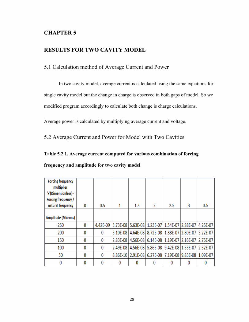
5.1 Calculation Method of Average Current and Power………………………………29
5.2 Average Current and Power for Model with Two Cavities……………………….29
Chapter 6 TRIALS WITH DIFFERENT INPUT PARAMETERS……………..32
6.1 Different Curve Patterns Observed ………………………………………………32
6.2 Different Input Parameters of System……………………………………………40
6.3 Trials with Different Plate Sizes and Gap between Plates………………………..40
6.4 Change in Input and Output Potentials…………………………………………….43
vi
Chapter 7 CONCLUSION AND RECOMMENDATIONS………………………46
7.1 Conclusion…………………………………………………………………………46
7.2 Future Work Recommendations…………………………………………………..46
REFERENCES………………………………………………………………….......47
Appendix 1: Matlab program for Model with Two Cavities …………………….50
1.1: Main Program for Model with Two Cavities ……………………………………50
1.2: Subroutine Program for Model with Two Cavities………………………….......52
Appendix 2: Matlab program for Model with Single Cavities……………………53
2.1: Main Program for Single Cavity Model…………………………………………53
2.2: Subroutine Program for Single Cavity Model…………………………………...55

vii
LIST OF FIGURE
Figure Page
1.3.1 Mass-spring-dashpot system arrangement……………………….…3
2.1.1 Single cavity variable parallel plate capacitor model……………....5
2.1.2 Stopper spring arrangement………………………………………...6
2.2.1 Variable parallel plate capacitor model with two cavities……….....7
2.3.1 Electric circuit of single cavity model……………………………...7
2.3.2 Electric circuit of two cavity model………………………………..8
2.6.1 Free body diagram of movable plate of single cavity model………10
2.6.2 Non dimensional ratio for gap between two plates…………….......14
2.7.1 Free body diagram of movable plate in two cavity model………...17
3.2.1 Simulation result for single cavity model…………………………20
3.2.2 Simulation result for model with two cavities..………………..…..22
4.2.1 Average current vs. amplitude vs. forcing frequency multiplier
graph for single cavity Model……………………………………..28
5.2.1 Average current vs. amplitude vs. forcing frequency multiplier
graph for two cavities Model……………………………………...30
6.1.1 Graph when no vibration force provided……………………….....33
6.1.2 Graph when small vibration force provided………………………33
6.1.3 Graph when vibration force provided is increased …………….....34
viii
6.1.4 Movable plate stuck to fixed plate…………………………………35
6.1.5 Regular repetitive pattern of plate movement……………………..36
6.1.6 Random pattern of plate movement……………………………….36
6.1.7 Upside double bounce repetitive pattern of plate movement……...37
6.1.8 Downside double bounce repetitive pattern of plate movement…..37
6.1.9 Upside and downside double bounce repetitive pattern of plate
movement………………………………………………………….38
6.1.10 Multiple bounce on both sides, repetitive pattern of plate
movement…………………………………………………………38
6.1.11 Different symbols used for different displacement waveforms…..39
6.1.12 Pattern of different displacement waveforms for different base
amplitude and forcing frequency combinations…………………..39
ix
LIST OF TABLES
Table Page
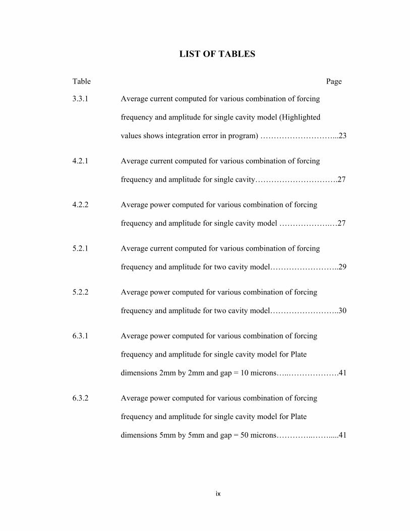
3.3.1 Average current computed for various combination of forcing
frequency and amplitude for single cavity model (Highlighted
values shows integration error in program) ………………………...23
4.2.1 Average current computed for various combination of forcing
frequency and amplitude for single cavity………………………….27
4.2.2 Average power computed for various combination of forcing
frequency and amplitude for single cavity model ……………….…27
5.2.1 Average current computed for various combination of forcing
frequency and amplitude for two cavity model……………………..29
5.2.2 Average power computed for various combination of forcing
frequency and amplitude for two cavity model……………………..30
6.3.1 Average power computed for various combination of forcing
frequency and amplitude for single cavity model for Plate
dimensions 2mm by 2mm and gap = 10 microns…..……………….41
6.3.2 Average power computed for various combination of forcing
frequency and amplitude for single cavity model for Plate
dimensions 5mm by 5mm and gap = 50 microns…………..…….....41

x
6.3.3 Average power computed for various combination of forcing
frequency and amplitude for model with two cavities for Plate
dimensions 2mm by 2mm and gap = 10 microns…………………...42
6.3.4 Average power computed for various combination of forcing
frequency and amplitude for model with two cavities for Plate
dimensions 5mm by 5mm and gap = 50 microns…………………...42
6.4.1.a Average current computed for various values of frequencies at
two fixed amplitude values for model with two cavities by
changing input and output potentials..………………………………43
6.4.1.b Average current computed for various values of frequencies at
two fixed amplitude values for model with two cavities by
changing input and output potentials……..…………………………43
6.4.2.a Average current computed for various values of Amplitude at
two fixed values of frequencies for two cavity model by
changing input and output potentials………………………………..44
6.4.2.b Average current computed for various values of Amplitude at
two fixed values of frequencies for two cavity model by
changing input and output potentials………………………………..44
1
CHAPTER 1
INTRODUCTION
1.1 Motivation for Research
In today’s world use of energy is going exponentially and prices of energy from
sources like coal, oil and natural gases are increasing in market. Conventional energy
sources like crude oil, coal and natural gas are major energy sources in our day to day life
but conventional energy takes thousands of years to reproduce. So production rate of
conventional energy sources is smaller than the consumption rate and will become extinct
after a few hundred years. Our future generation will not have any conventional energy
sources to use. That is why; the focus on other options of energy sources, i.e.
nonconventional energy sources has increased in last few years. Non-conventional energy
sources include solar, wind, tide etc. as energy sources but there is one more important
energy source available in nature i.e. vibration energy. In environment, undamped and
unwanted vibrations are abundantly available like in industry, construction site, machines
produces lot of unwanted vibration when they are in use. In such case vibration based
energy scavengers are considered to be ideal power sources for low power devices. Now
a day’s, use of mobile and electronic devices increased and charging of these devices
consumes lot of electric energy. Imagine, you are travelling in car and we have device
which converts vibrations produce from car into electric energy. Then we can charge all
these electronic devices for free while travelling.

2
1.2 Literature Review
MicroElectroMechanical System (MEMS) is a combination of electrical and
mechanical systems and size of this system is in micrometers. Converting vibration
energy into electrical energy can be done using three methods 1.Inductive, 2.Piezoelectric
and 3.Capacitive. The variable capacitive method is considered as easy and capable of
miniaturization but it needs a voltage bias for conversion process [5].
The work related to variable parallel plate capacitor was more focused on single
cavity model but in this work we analyzed the simulation of model with single cavity and
two cavities which leads to one variable capacitor and two variable capacitors
respectively. This is the first time we did study of MEMS parallel plate capacitor Model
with two cavities. The model design and arrangement, electric circuit and numerical
solution for both models are discussed in this paper. We will compare the dynamics and
simulation output for single cavity and two cavity model. Also we analyses the
performance of both models to generate output current and power.
The activation force for these models is the vibration force so we tested both
models for different combination of forced frequencies and base amplitude and different
results are presented in this paper.

3
1.3 Concept of Basic Design
The concept of basic design for MEMS parallel plate capacitor model is based on
mass-spring-dashpot system ( Figure 1.3.1)
Figure 1.3.1. Mass-spring-dashpot system arrangement
In spring- mass- dashpot system, mass is suspended on spring and mass moves
with vibrations provided to mass as force of excitation. Dashpot works as damping force
to the system.
Here,
Mass = m, Spring constant = k, Damping constant = c and Displacement of mass = x
In this system, mass is attached to Hook’s law of spring,
So,
Spring force = -kx………………………………………………(1)
Damping force = ………………………………….……..(2)
4
Now, From Newton’s second law, the acceleration ‘a’ of a body is parallel and
directly proportional to the net force ‘f’ and inversely proportional to the mass ‘m’ [11]
i.e.
∑ ……………………………………….…..(3)
For given system (Figure1),
……………………………………(4)
By rearranging and divided by m,
0………………………………….(5)
This gives the governing equation for Mass spring dashpot system. Similarly,
Governing equation for MEMS parallel plate capacitor models with single cavity and two
cavities are computed and numerical solutions are computed using Matlab program.
5
CHAPTER 2
MATHEMATICAL MODEL OF DEVICE
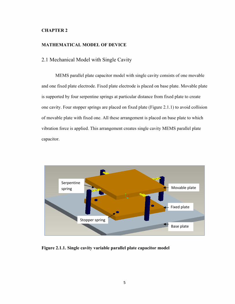
2.1 Mechanical Model with Single Cavity
MEMS parallel plate capacitor model with single cavity consists of one movable
and one fixed plate electrode. Fixed plate electrode is placed on base plate. Movable plate
is supported by four serpentine springs at particular distance from fixed plate to create
one cavity. Four stopper springs are placed on fixed plate (Figure 2.1.1) to avoid collision
of movable plate with fixed one. All these arrangement is placed on base plate to which
vibration force is applied. This arrangement creates single cavity MEMS parallel plate
capacitor.
Figure 2.1.1. Single cavity variable parallel plate capacitor model
Base plate
Movable plate
Fixed plate
Serpentine
spring
Stopper spring

6
To avoid the collision of movable plate with fixed one, we placed four stopper
springs on fixed plate at equal distance from four corners of plate. The length of stopper
spring is considered as 0.2 times the gap between the two plates (Figure 2.1.2).
Figure 2.1.2. Stopper spring arrangement
2.2 Mechanical Model with Two Cavities
This model consists of two fixed plate electrodes and one movable plate electrode
placed in between two fixed one. Movable plate is supported by four serpentine springs.
Four stopper springs are placed on each fixed plate (Figure 2.2.1) to avoid collision of
movable plate with fixed plates. All these arrangement is placed on base plate and
vibration force is applied to base plate. This model leads to two variable capacitors with
gap1 and gap2 (Figure 2.3.2).
7
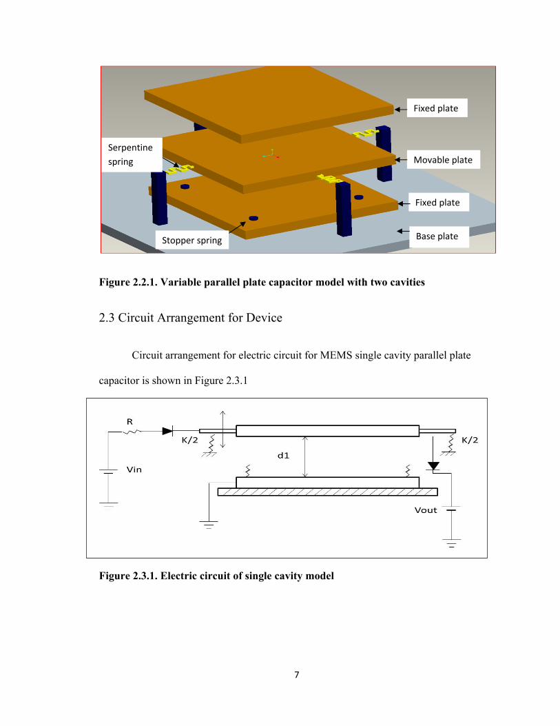
Figure 2.2.1. Variable parallel plate capacitor model with two cavities
2.3 Circuit Arrangement for Device
Circuit arrangement for electric circuit for MEMS single cavity parallel plate
capacitor is shown in Figure 2.3.1
Figure 2.3.1. Electric circuit of single cavity model
Fixed plate
Stopper spring
Serpentine
spring Movable plate
Fixed plate
Base plate
8
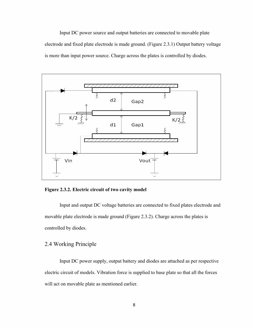
Input DC power source and output batteries are connected to movable plate
electrode and fixed plate electrode is made ground. (Figure 2.3.1) Output battery voltage
is more than input power source. Charge across the plates is controlled by diodes.
Figure 2.3.2. Electric circuit of two cavity model
Input and output DC voltage batteries are connected to fixed plates electrode and
movable plate electrode is made ground (Figure 2.3.2). Charge across the plates is
controlled by diodes.
2.4 Working Principle
Input DC power supply, output battery and diodes are attached as per respective
electric circuit of models. Vibration force is supplied to base plate so that all the forces
will act on movable plate as mentioned earlier.

9
We assume that the package containing the capacitors is subject to sinusoidal
displacement. Movable plate will start moving up and down due to vibration force and
because of the motion the gap between the movable plate electrode and fixed plate
electrode will change which leads to change in charge across plates. As distance between
two plates decreases charge across the plate decreases and as distance increases charge
increases almost instantaneously.
This leads to change in voltage and after reaching to pull down voltage, plate will
start striking on stopper spring to avoid collision between electrodes. This cycle will
continue to repeat until the forced vibrations are applied. This dynamics effect we can
check in our simulation results (Figure 3.2.1, 3.2.2).
The charges are controlled by diodes to achieve the pumping effect from low
voltage source to high voltage battery and ultimately to charge the output battery.
So using variable parallel plate capacitor we converted vibration energy into
electrical energy.
Through charging and discharging, the capacitive plates exchange energy with the
electrical components both upstream and downstream; mechanical energy is dispensed in
the process.
2.5 Symbols and Terminology
In this system, following symbols are used
V = Voltage across plate

10
ε = permittivity,
A= c/s area of plate
= gap between plates at equilibrium, = gap between plates at time t
m = mass of movable plate,
k= total spring force
c= Air damping coefficient
=Electrostatic force, = spring force, =Inertia force
2.6 Forces acting on Movable Plate and Governing Equations of Motion for
Model with Single Cavity
Figure 2.6.1. Free body diagram of movable plate of single cavity model
The moving plate is subjected to inertia force from vibrating base plate, spring
force from serpentine springs, air damping force and the electrostatic force due to charge
in capacitor (Figure 2.6.1). Equations for all these forces are given as follows,
11
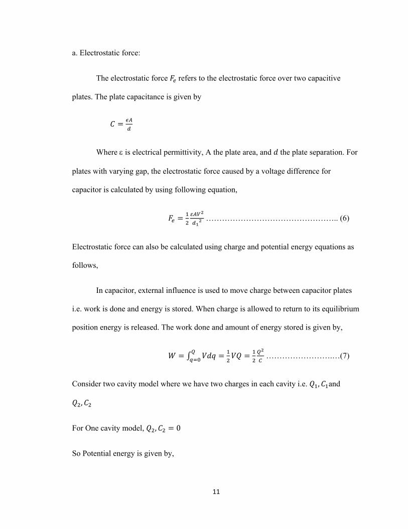
a. Electrostatic force:
The electrostatic force refers to the electrostatic force over two capacitive
plates. The plate capacitance is given by
Where is electrical permittivity, A the plate area, and the plate separation. For
plates with varying gap, the electrostatic force caused by a voltage difference for
capacitor is calculated by using following equation,
………………………………………….. (6)
Electrostatic force can also be calculated using charge and potential energy equations as
follows,
In capacitor, external influence is used to move charge between capacitor plates
i.e. work is done and energy is stored. When charge is allowed to return to its equilibrium
position energy is released. The work done and amount of energy stored is given by,
…………………….…(7)
Consider two cavity model where we have two charges in each cavity i.e. , and
,
For One cavity model, , 0
So Potential energy is given by,
12
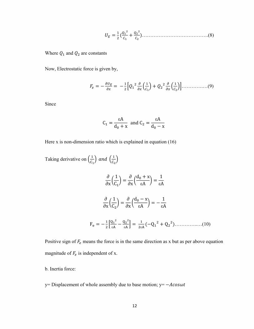
………………………………….(8)
Where and are constants
Now, Electrostatic force is given by,
………….…(9)
Since
CεA
d xandC
εAd x
Here x is non-dimension ratio which is explained in equation (16)
Taking derivative on
∂∂x
1C
∂∂x
d xεA
1εA
∂∂x
1C
∂∂x
d xεA
1εA
Fε ε
ε
Q Q …………..…(10)
Positive sign of means the force is in the same direction as x but as per above equation
magnitude of is independent of x.
b. Inertia force:
y= Displacement of whole assembly due to base motion; y=
13
………………….... (11)
c. Spring force
……………………………… (12)
In spring force, additional stopper spring force will be added
To avoid the collision between the plates, we placed four stoppers on the fixed
plate. The moving plate makes contact with the stopper when its displacement is 80% of
the initial gap. The stopper is modeled as a very stiff spring whose spring constant is
1000 times of the plate suspension. Therefore, the stopper acts like a nonlinear spring and
its force can be written as shown below.
In this case we considered stopper length is 0.2 times the gap between two plates
and the stiffness is 2000 times stiffness of serpentine spring ‘k’
StopperspringforceF 1000*k* max d d 0.8 )
d. Air damping force
Air damping force = ………………………….….. (13)
If the device is sealed in a vacuum, the mechanical damping can be negligible.
Using the Newton’s second law of motion, the equation for system is given as below,
…………….……… (14)
Now, to simplify this equation, we introduce some terms.
14
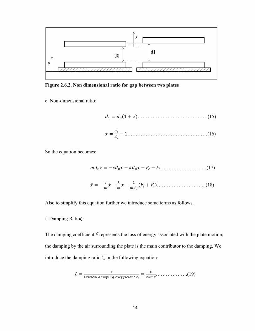
Figure 2.6.2. Non dimensional ratio for gap between two plates
e. Non-dimensional ratio:
1 ……………………………………(15)
1…………………………………………(16)
So the equation becomes:
…………………….…(17)
………………………...(18)
Also to simplify this equation further we introduce some terms as follows.
f. Damping Ratio :
The damping coefficient c represents the loss of energy associated with the plate motion;
the damping by the air surrounding the plate is the main contributor to the damping. We
introduce the damping ratio ζ, in the following equation:
√……………….(19)

15
√ 2 ……………………………….(20)
Substituting this term in equation (18) we get,
2 ……………………….(21)
g. Pull down voltage :
Since the gap is varying, this force is dependent on the plate displacement x. When the
gap decreases, the electrostatic force increases. This force is nonlinear, i.e. the increase is
not proportional to the displacement. The increase may overwhelm the restoring force of
the elastic support to cause the gap to collapse. When this is caused by the gradual
increase of the voltage, a critical voltage, called the pull down voltage, is known to exist:
, where …………………….(22)
Where and are the gap and capacitance at static equilibrium when no voltage is
applied.
The electrostatic force is determined by the voltage on the capacitor. The voltage is
calculated from the charge on the plate:
The charge on the plate can be determined by keeping track of the current flowing
in and out the capacitor. However, since the plate capacitance is very small, charging and
discharging time is very short. Keeping track of the current flow would require additional
differential equation. The numerical solution of this additional equation would require
extremely small integration time steps to prevent numerical instability. Since the short
16
charging and discharging time can be ignored, we assume that the charge on the plate is
constant when no charging or discharging takes place. That is, Q is constant if
. By ignoring the charging and discharging time, we set up the following
limitations on the voltage on the capacitor:
min And max .
The above limitations are imposed at the end of each time integration step. If the voltage
exceeds , we calculate the excess electric charge which is moved to the battery .
If the voltage is below , is reset to .
h. Calculating spring constant using
…………………………………..…(23)
We consider the pull down voltage as fixed value and from that we calculate the spring
constant.
Now,
And ∗ , Stopper spring force=
Putting in equation (21), we get:
2 …………………………(24)
So simplified equation becomes,
2 ………….……(25)
17
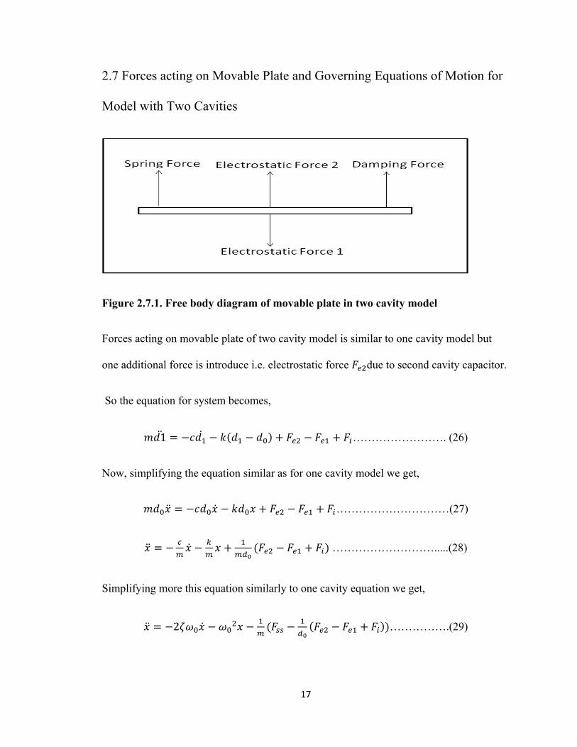
2.7 Forces acting on Movable Plate and Governing Equations of Motion for
Model with Two Cavities
Figure 2.7.1. Free body diagram of movable plate in two cavity model
Forces acting on movable plate of two cavity model is similar to one cavity model but
one additional force is introduce i.e. electrostatic force due to second cavity capacitor.
So the equation for system becomes,
1 ……………………. (26)
Now, simplifying the equation similar as for one cavity model we get,
…………………………(27)
……………………….....(28)
Simplifying more this equation similarly to one cavity equation we get,
2 …………….(29)
18
CHAPTER 3
NUMERICAL SOLUTION OF THE EQUATIONS OF MOTION
3.1 Dimensions of Model
Matlab programming is used to find the numerical solutions of governing equations for
MEMS parallel plate capacitor models with single and two cavities. To run matlab
programming, some input parameter values are need to be consider as fixed as follows,
Permittivity constant = 8.85*10^-12
Mass of moving plate = Density of material * Volume of plate
Density of Material= 8912kg per cubic meter for Nickel
Volume of plate= Area of plate (Length *width) * thickness of plate
Pull down voltage = 20V
Capacitance = Permittivity constant* area of plate / gap between plates
Input Potential = 15V
Output Potential = 45V
Natural Frequency = 164.8223 hertz
19
3.2 Implementation of Numerical Equation
Using the equations of forces for movable plate we developed Matlab program
pump.m and pumpsub2.m (Single cavity -Appendix II, Two cavities- Appendix I) to
simulate the system and we got following results.
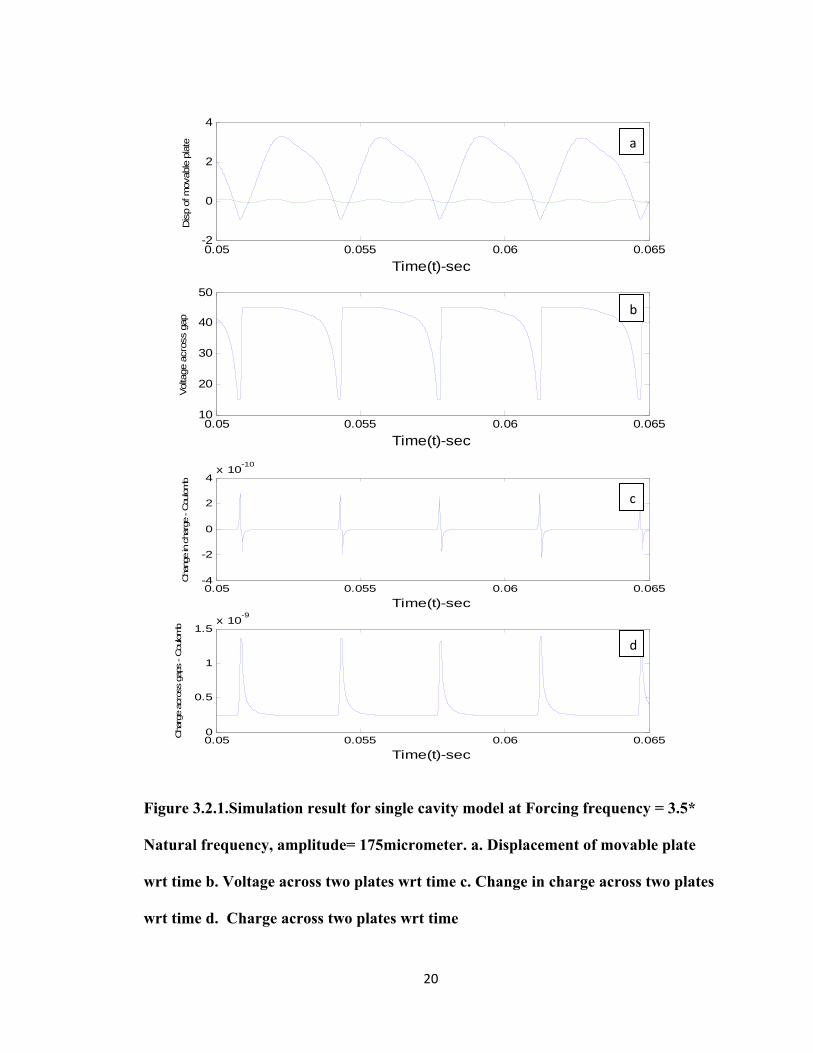
For single cavity model, movable plate will move up and down and after some
time it will start striking on stopper spring at bottom only. It does not have any limit in up
direction because of stopper springs.
From Figure 3.2.1 a, we can observe the motion and position of movable plate
and in figure 3.2.1b, we can observe the change in voltage across the plates as position of
plates changes. As plate moves down, voltage decreases and as plate moves in up
direction after striking to stopper springs voltage increases almost instantaneously.
Using the plate position we have plotted charge and change in charge across both plates.
20
Figure 3.2.1.Simulation result for single cavity model at Forcing frequency = 3.5*
Natural frequency, amplitude= 175micrometer. a. Displacement of movable plate
wrt time b. Voltage across two plates wrt time c. Change in charge across two plates
wrt time d. Charge across two plates wrt time
0.05 0.055 0.06 0.065-2
0
2
4
Time(t)-sec
Dis
p of
mov
able
pla
te
0.05 0.055 0.06 0.06510
20
30
40
50
Time(t)-sec
Vol
tage
acr
oss
gap
0.05 0.055 0.06 0.065-4
-2
0
2
4x 10
-10
Time(t)-sec
Cha
nge
in c
harg
e - Cou
lom
b
0.05 0.055 0.06 0.0650
0.5
1
1.5x 10
-9
Time(t)-sec
Cha
rge
acro
ss g
aps
- Cou
lom
b
a
b
c
d

21
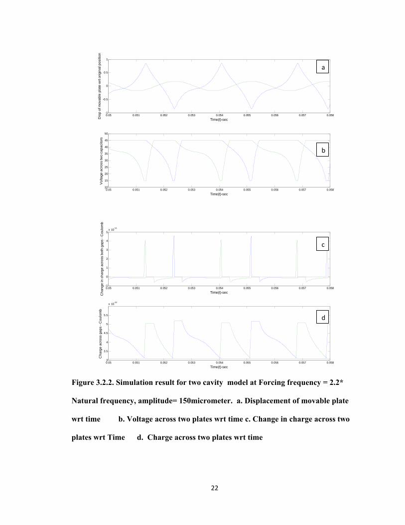
In two cavity model, stopper springs are placed on both fixed plate electrodes. So
as voltage across plates reaches to pull down voltage, plate start striking on stopper
springs. We can observe this effect in figure 3.2.2.a.
Two cavity models have two gaps which lead to two capacitors. From figure
3.2.2.b we can observe the change in voltage across the gaps, (Figure 3.2.2.b only, blue
color- bottom gap voltage, and green color- upper gap voltage). As plate moves down,
the voltage across the bottom gap decreases but on the other hand this leads to increase in
distance between electrodes of upper gap which increases the voltage for upper gap
capacitor and vice versa.
22
Figure 3.2.2. Simulation result for two cavity model at Forcing frequency = 2.2*
Natural frequency, amplitude= 150micrometer. a. Displacement of movable plate
wrt time b. Voltage across two plates wrt time c. Change in charge across two
plates wrt Time d. Charge across two plates wrt time
0.05 0.051 0.052 0.053 0.054 0.055 0.056 0.057 0.058-1
-0.5
0
0.5
1
Time(t)-secDis
p o
f mo
vab
le p
late
wrt
ori
gina
l pos
ition
0.05 0.051 0.052 0.053 0.054 0.055 0.056 0.057 0.05810
15
20
25
30
35
40
45
50
Time(t)-sec
Vo
ltage
acr
oss
two
ca
pac
itors
0.05 0.051 0.052 0.053 0.054 0.055 0.056 0.057 0.058-1
0
1
2
3
4
5x 10
-11
Time(t)-sec
Ch
ang
e in
ch
arg
e a
cro
ss b
oth
gap
s -
Cou
lom
b
0.05 0.051 0.052 0.053 0.054 0.055 0.056 0.057 0.0583
3.5
4
4.5
5
5.5
x 10-10
Time(t)-sec
Cha
rge
acro
ss g
aps
- C
oul
omb
a
b
c
d
23
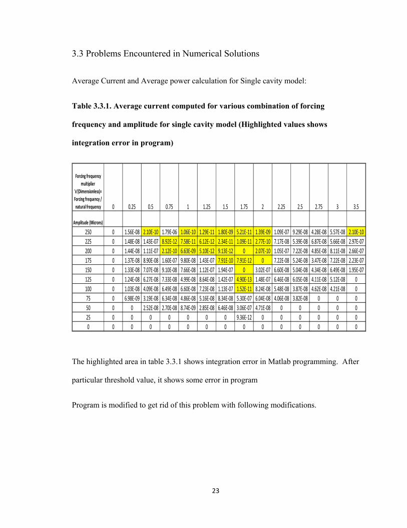
3.3 Problems Encountered in Numerical Solutions
Average Current and Average power calculation for Single cavity model:
Table 3.3.1. Average current computed for various combination of forcing
frequency and amplitude for single cavity model (Highlighted values shows
integration error in program)
Forcing frequency
multiplier
'x'(Dimensionless)=
Forcing frequency /
natural frequency 0 0.25 0.5 0.75 1 1.25 1.5 1.75 2 2.25 2.5 2.75 3 3.5
Amplitude (Microns)
250 0 1.56E‐08 2.10E‐10 1.79E‐06 1.06E‐10 1.29E‐11 1.80E‐09 5.21E‐11 1.39E‐09 1.09E‐07 9.29E‐08 4.28E‐08 5.57E‐08 2.10E‐10
225 0 1.48E‐08 1.43E‐07 8.92E‐12 7.58E‐11 6.12E‐12 2.34E‐11 1.09E‐11 2.77E‐10 7.17E‐08 5.39E‐08 6.87E‐08 5.66E‐08 2.97E‐07
200 0 1.44E‐08 1.11E‐07 2.12E‐10 6.63E‐09 5.10E‐12 9.13E‐12 0 2.07E‐10 1.05E‐07 7.22E‐08 4.85E‐08 8.11E‐08 2.66E‐07
175 0 1.37E‐08 8.90E‐08 1.60E‐07 9.80E‐08 1.43E‐07 7.91E‐10 7.91E‐12 0 7.22E‐08 5.24E‐08 3.47E‐08 7.22E‐08 2.23E‐07
150 0 1.33E‐08 7.07E‐08 9.10E‐08 7.66E‐08 1.12E‐07 1.94E‐07 0 3.02E‐07 6.60E‐08 5.04E‐08 4.34E‐08 6.49E‐08 1.95E‐07
125 0 1.24E‐08 6.27E‐08 7.33E‐08 4.99E‐08 8.64E‐08 1.42E‐07 4.90E‐13 1.48E‐07 6.46E‐08 6.05E‐08 4.11E‐08 5.12E‐08 0
100 0 1.03E‐08 4.09E‐08 6.49E‐08 6.60E‐08 7.23E‐08 1.13E‐07 1.52E‐11 8.24E‐08 5.48E‐08 3.87E‐08 4.62E‐08 4.21E‐08 0
75 0 6.98E‐09 3.19E‐08 6.34E‐08 4.86E‐08 5.16E‐08 8.34E‐08 5.30E‐07 6.04E‐08 4.06E‐08 3.82E‐08 0 0 0
50 0 0 2.52E‐08 2.70E‐08 8.74E‐09 2.85E‐08 6.46E‐08 3.06E‐07 4.71E‐08 0 0 0 0 0
25 0 0 0 0 0 0 0 9.36E‐12 0 0 0 0 0 0
0 0 0 0 0 0 0 0 0 0 0 0 0 0 0
The highlighted area in table 3.3.1 shows integration error in Matlab programming. After
particular threshold value, it shows some error in program
Program is modified to get rid of this problem with following modifications.

24
Concept of Impact and Coefficient of Restitution:
In our model, moving plate will collide on stopper spring but as moving plate will
pushes stopper spring, Stopper spring will become stiffer and will stop further
compression.
So, here spring force due to serpentine springs =
And stopper spring force is given by,
Stiffness = k2 = 1000*k
In our model, Stopper spring is at distance of 80% from original position of movable
plate. So stopper force will be as follows,
Nonlinear spring equation represents the stopper.
If x < -0.8;
| || 1 0.8| ……………………….(30)
else if x > 0.8;
| || 1 0.8|………………………..(31)
else,
0…………………………………………..(32)
For one cavity only equation 30 and 32 were used.
25
In initial programming, we considered simulation of stopper spring through the
duration when the stopper spring is acting but we considered this movement as
instantaneously.
In this concept we are adding coefficient of restitution (COR). COR of an object
is a frictional value representing the ratio of velocities after and before an impact. For a
COR = 0, the object effectively "stops" at the surface with which it collides, not bouncing
at all. For COR=1, object collides elastically and an object with a COR < 1 collides
inelastically.
Where, v = scalar velocity of object after impact
u= scalar velocity of object before impact
Finally, by reducing step size i.e. from 10^-5 step size to 10^-6 step size.
Results for modified program with concept of impact, coefficient of restitution and step
size computed.
26
CHAPTER 4
RESULTS FOR SINGLE CAVITY MODEL
4.1 Calculation method of Average Current and Power
Using Matlab program developed for movable plate in MEM system and graphs are
plotted for charge and change in charge across both plates.
Using this data we have calculated average current using following formula.
Current (I) =
………………………………………………(33)
And Power (P) = current *voltage = VI ………………………………………….(34)
In Matlab program this equations are used and Average current and average power are
calculated at different combination of forcing frequency and amplitudes.
4.2 Average Current and Power for Model with Single Cavity
Average Current and Average power calculation for Single cavity model:

27
Table 4.2.1. Average current computed for various combination of forcing
frequency and amplitude for single cavity Model
Table 4.2.2. Average power computed for various combination of forcing frequency
and amplitude for single cavity model
28
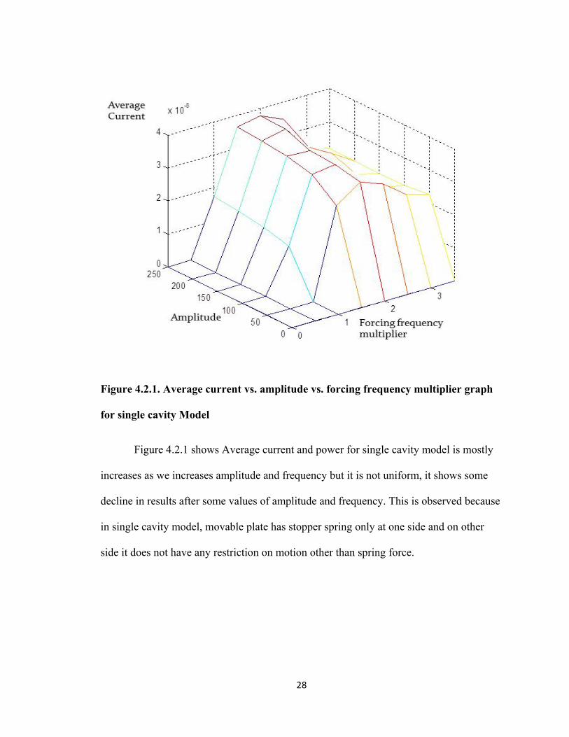
Figure 4.2.1. Average current vs. amplitude vs. forcing frequency multiplier graph
for single cavity Model
Figure 4.2.1 shows Average current and power for single cavity model is mostly
increases as we increases amplitude and frequency but it is not uniform, it shows some
decline in results after some values of amplitude and frequency. This is observed because
in single cavity model, movable plate has stopper spring only at one side and on other
side it does not have any restriction on motion other than spring force.
29
CHAPTER 5
RESULTS FOR TWO CAVITY MODEL
5.1 Calculation method of Average Current and Power
In two cavity model, average current is calculated using the same equations for
single cavity model but the change in charge is observed in both gaps of model. So we
modified program accordingly to calculate both change is charge calculations.
Average power is calculated by multiplying average current and voltage.
5.2 Average Current and Power for Model with Two Cavities
Table 5.2.1. Average current computed for various combination of forcing
frequency and amplitude for two cavity model

30
Table 5.2.2. Average power computed for various combination of forcing frequency
and amplitude for two cavity model
Figure 5.2.1. Average current vs. amplitude vs. forcing frequency multiplier graph
for two cavities Model
31
From graphs for average current and power, it is observed that as forcing
frequency and / or base amplitude increases, average current and power also increases.
It is observed that, model with two cavities gives better results than model with
single cavity. In single cavity model average current and power do not increase uniformly
as it does in model with two cavities. The reason behind this is that in model with two
cavities, movement of movable plate is restricted on both sides using stopper springs. So
as forcing frequency and/or amplitude increases, movement of plate increases. Movable
plate strikes more frequently in one cycle of sinusoidal wave of forcing frequency. In
model with one cavity, movement of movable plate is restricted only on one side. So as
forcing frequency and/or amplitude increases, plate strikes on one side but keep flying on
other side. So after particular values of amplitude and frequency it does not show any
improvement in results.

32
CHAPTER6
TRIALS WITH DIFFERENT INPUT PARAMETES
6.1 Different Curve Patterns Observed
Different simulation curves observed for different combination for dynamic
forces. To check the effect of vibration force we computed average current and power for
different combination of forced frequencies and amplitude.
Different trails were conducted for various combination of forcing frequency and
amplitude and different waveforms were observed for displacement of movable plate.
Because of different plate displacement the average current and power also changes. So
its effect on average current were studied and it is observed that at some particular
displacement waveform of plate we get more average current compare to others.
Different waveforms observed at different combination of frequency- amplitude
and average current computed for particular waveform are mentioned below.

33
Figure 6.1.1. Graph when no vibration force provided
i.e. at 0 amplitude and forcing frequency is 0 times natural frequency. V 5,
V 25. Simulation shows no change and hence no energy harvesting.
Figure 6.1.2 Graph when small vibration force provided
0 0.002 0.004 0.006 0.008 0.01 0.012 0.014 0.016 0.018 0.02-1
0
1
Time(t)-sec
Displac
emen
t
0 0.002 0.004 0.006 0.008 0.01 0.012 0.014 0.016 0.018 0.0214
15
16
Time(t)-sec
Volta
ge
0 0.002 0.004 0.006 0.008 0.01 0.012 0.014 0.016 0.018 0.02-1
0
1
Time(t)-sec
Cha
nge
in c
harg
e - Cou
lom
b
0 0.002 0.004 0.006 0.008 0.01 0.012 0.014 0.016 0.018 0.02-0.5
0
0.5
Time(t)-sec
Displac
emen
t
0 0.002 0.004 0.006 0.008 0.01 0.012 0.014 0.016 0.018 0.025
6
7
Time(t)-sec
Volta
ge
0 0.002 0.004 0.006 0.008 0.01 0.012 0.014 0.016 0.018 0.02-1
0
1
Time(t)-sec
Cha
nge
in c
harg
e - Cou
lom
b
34
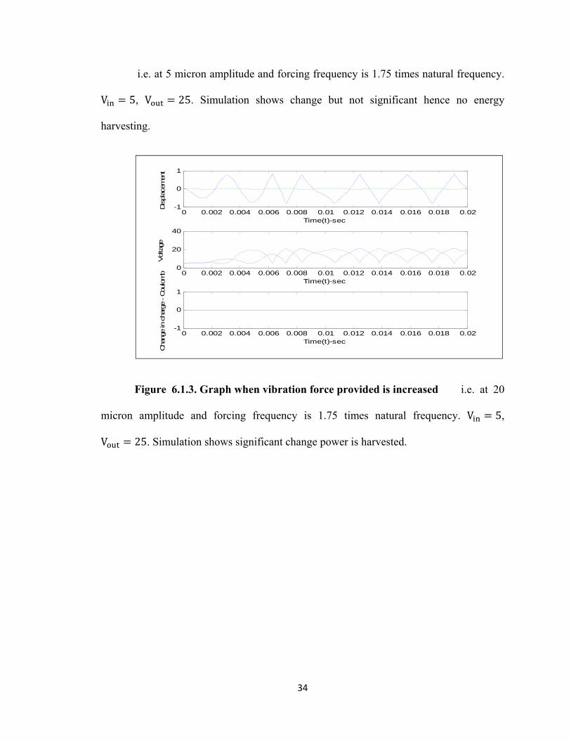
i.e. at 5 micron amplitude and forcing frequency is 1.75 times natural frequency.
V 5, V 25. Simulation shows change but not significant hence no energy
harvesting.
Figure 6.1.3. Graph when vibration force provided is increased i.e. at 20
micron amplitude and forcing frequency is 1.75 times natural frequency. V 5,
V 25. Simulation shows significant change power is harvested.
0 0.002 0.004 0.006 0.008 0.01 0.012 0.014 0.016 0.018 0.02-1
0
1
Time(t)-sec
Dis
plac
emen
t
0 0.002 0.004 0.006 0.008 0.01 0.012 0.014 0.016 0.018 0.020
20
40
Time(t)-sec
Vol
tage
0 0.002 0.004 0.006 0.008 0.01 0.012 0.014 0.016 0.018 0.02-1
0
1
Time(t)-sec
Cha
nge
in c
harg
e - Cou
lom
b

35
Figure 6.1.4. Movable plate stuck to fixed plate
In some cases movable plate get stuck at either of stopper spring location. The
attraction between two plates is more and vibration force in not significant enough to
move movable plate against it. At 10 micron amplitude and forcing frequency is 1.75
times natural frequency. V 15, V 25. Simulation shows movable plate get stuck
at lower stopper spring plate and hence no energy harvesting possible.
In Initial programming, many waveform patterns are found common as follows,
0 0.002 0.004 0.006 0.008 0.01 0.012 0.014 0.016 0.018 0.02-1
0
1
Time(t)-sec
Dis
plac
emen
t
0 0.002 0.004 0.006 0.008 0.01 0.012 0.014 0.016 0.018 0.0215
20
25
Time(t)-sec
Vol
tage
0 0.002 0.004 0.006 0.008 0.01 0.012 0.014 0.016 0.018 0.02-1
0
1
Time(t)-sec
Cha
nge
in c
harg
e - Cou
lom
b
36
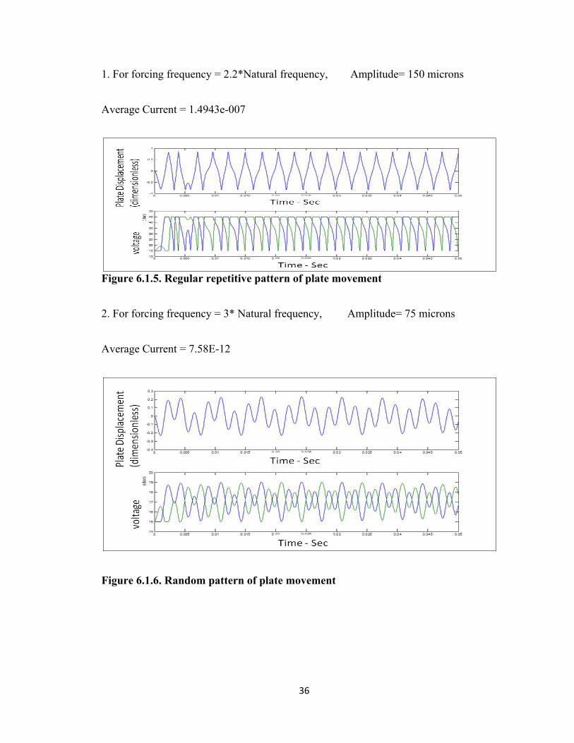
1. For forcing frequency = 2.2*Natural frequency, Amplitude= 150 microns
Average Current = 1.4943e-007
Figure 6.1.5. Regular repetitive pattern of plate movement
2. For forcing frequency = 3* Natural frequency, Amplitude= 75 microns
Average Current = 7.58E-12
Figure 6.1.6. Random pattern of plate movement

37
3. For forcing frequency =1.75* Natural frequency, Amplitude= 100 microns
Average Current = 1.1284e-007
Figure 6.1.7. Upside double bounce repetitive pattern of plate movement
4. For forcing frequency = 2*natural frequency, Amplitude=150 microns
Average Current =1.3973e-007
Figure 6.1.8. Downside double bounce repetitive pattern of plate movement

38
5. For forcing frequency = 1.5* natural frequency, Amplitude= 225 microns
Average Current =1.0802e-007
Figure 6.1.9. Upside-downside double bounce repetitive pattern of plate movement
6. For forcing frequency =0.75*natural frequency, Amplitude= 150 microns
Average Current =3.6274e-008
Figure 6.1.10. Multiple bounce on both sides, repetitive pattern of plate movement
It is observed that for displacement motion of movable plate observed in first waveform
(Figure 6.1.5) gives more output average current compare to others.
39
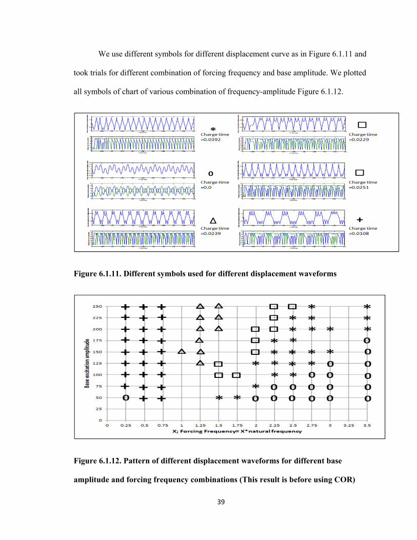
We use different symbols for different displacement curve as in Figure 6.1.11 and
took trials for different combination of forcing frequency and base amplitude. We plotted
all symbols of chart of various combination of frequency-amplitude Figure 6.1.12.
Figure 6.1.11. Different symbols used for different displacement waveforms
Figure 6.1.12. Pattern of different displacement waveforms for different base
amplitude and forcing frequency combinations (This result is before using COR)

40
It is observed that the some combinations of forcing frequency and base amplitude gives
more average current compare to others and this patterns found in particular region of
forcing frequency and amplitude.
6.2 Different Input Parameters of System
MEMS parallel plate capacitor model with single cavity and two cavities,
numerical solutions are found out by solving governing equations using Matlab
programming. These equations has many variables, so to solve these equations, some
parameters needs to be consider as fixed values and only few parameters as consider as
variable like forcing frequency and amplitude values.
To check the effect of other parameters like plate size, input and out voltages, gap
between two plates etc. by considering as variable, different trials were conducted.
6.3 Trials with Different Plate Sizes and Gap between Plates
In original programming, plate size is considered as 5mm*5mm, to see the effect of plate
size; plate size is reduced to 2mm*2mm.
Also Initial gap between two plates is considered as a fixed value of 50micrometer but to
check the effect, it is changed to 10 micrometers.

41
Table 6.3.1. Average power computed for various combination of forcing frequency
and amplitude, single cavity model with Plate dimension 2mm by2mm and gap 10
microns
Table 6.3.2. Average power computed for various combination of forcing frequency
and amplitude for single cavity model with Plate dimensions 5mm by 5mm and gap
50 microns
42
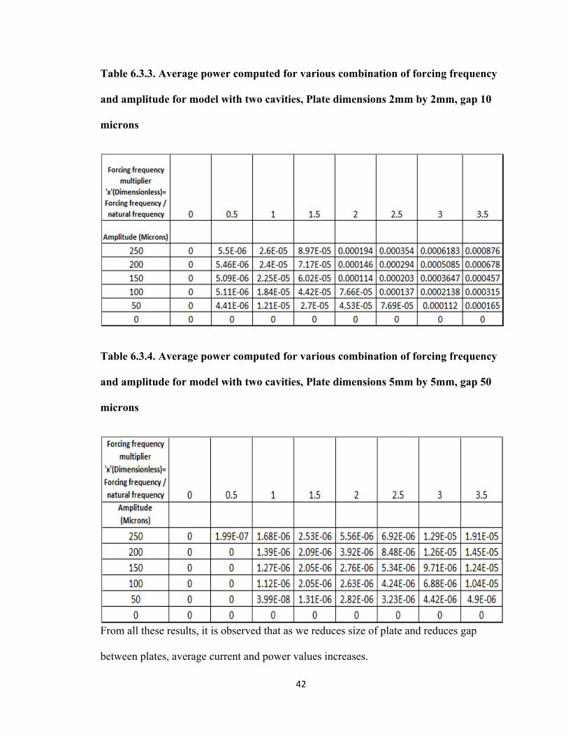
Table 6.3.3. Average power computed for various combination of forcing frequency
and amplitude for model with two cavities, Plate dimensions 2mm by 2mm, gap 10
microns
Table 6.3.4. Average power computed for various combination of forcing frequency
and amplitude for model with two cavities, Plate dimensions 5mm by 5mm, gap 50
microns
From all these results, it is observed that as we reduces size of plate and reduces gap
between plates, average current and power values increases.
43
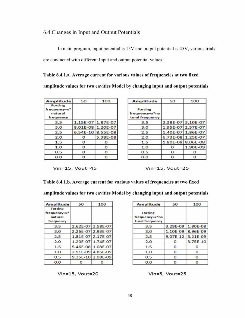
6.4 Changes in Input and Output Potentials
In main program, input potential is 15V and output potential is 45V, various trials
are conducted with different Input and output potential values.
Table 6.4.1.a. Average current for various values of frequencies at two fixed
amplitude values for two cavities Model by changing input and output potentials
Table 6.4.1.b. Average current for various values of frequencies at two fixed
amplitude values for two cavities Model by changing input and output potentials
44
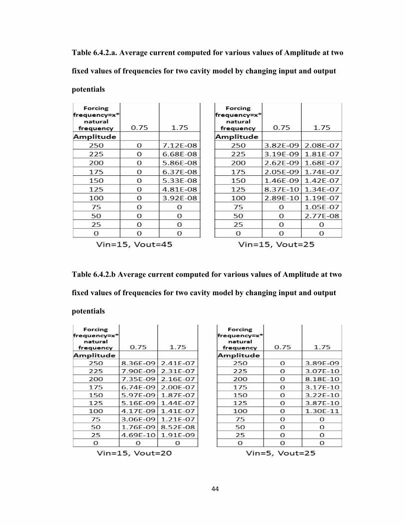
Table 6.4.2.a. Average current computed for various values of Amplitude at two
fixed values of frequencies for two cavity model by changing input and output
potentials
Table 6.4.2.b Average current computed for various values of Amplitude at two
fixed values of frequencies for two cavity model by changing input and output
potentials

45
So from above tables it is observed that, if difference between input and output
potential is more, at lower forcing frequency average current is zero at all amplitudes. If
difference is small, average current can be calculated at lower forcing frequency. As we
reduces the value of output voltage, average current increases
If we reduces input potential, at lower frequencies average current is zero and
average current is lower at higher frequency. When difference between input and output
potential is more, average current at lower frequencies cannot be calculated but as we
reduces that difference, we can compute the average current at lower frequencies too.
Keeping input potential same and just by reducing input potential i.e. reducing the
difference between input and output potential we get better result.
46
CHAPTER 7
CONCLUSION AND RECOMMENDATIONS
7.1 Conclusion
Two different models for variable parallel plate capacitor were proposed and
workings of both models were discussed for stepping up the voltage and power
harvesting. Simulation for movable plate electrode estimated and average current and
power computed for various combination of forcing frequencies and amplitude. Different
trials with various input parameters conducted and compared. MEMS Model with two
cavities gives better results than single cavity model. From different trials, we can
conclude that as we increase forcing frequency and/or amplitude of vibration we get
better results. Also better results can be generated by reducing the difference between
input and output potential, by reducing the plate size and by reducing the gap between the
two plates.
7.2 Future Work Recommendations
In future, trials with other input parameters should be conducted. Generalized
equation between input parameter and output needs to be generated. In this study motion
of plate is considered in one axis of direction but in future tilting effect of plate due to
uneven forces needs to be studied.

47
REFERENCES
[1] P.D. Mitcheson, P. Miao, B.H. Stark, E.M. Yeatman, A.S. Holmes, T.C. Green,
2004, “MEMS electrostatic micropower generator for low frequency operation” ,
Sensors and Actuators A 115(2004) 523-529, Department of Electrical and
Electronic Engineering, Imperial college London, London, UK
[2] P.D. Mitcheson, B.H.Stark, P.Miao, E.M. Yeatman, A.S.Holems, T.C.Green,
“Analysis and optimization of MEMS electrostatic on-chip power supply for self-
powering of slow- moving sensors” 48-51,Department of Electrical and
Electronic Engineering, Imperial College London, London, UK
[3] E.M. Yeatman, 2007, “Applications of MEMS in power sources and circuits” IOP
Publishing J. Micromech, Microeng. 17(2007) S184-S188, Department of
Electrical and Electronic Engineering, Imperial College London, London, UK
[4] Masayuki Miyazaki, Hidetoshi Tanaka, Goichi Ono, Tomohiro Nagano, Norio
Ohkubo, Takayuki Kawahara, Kazuo Yano, 2003, “Electric- energy generation
using variable- capacitive resonator for power-free LSI: efficiency analysis and
fundamental experiment” ACM 1-58113-682-X/03/008, 193-198, Hitachi Ltd.,
Central Research Laboratory, Kokubunji, Tokyo, Japan.

48
[5] Fabio Peano and TizianaTambosso, 2004-5, “Design and optimization of MEMS
electret-based capacitive energy scavenger”, Journal of Microelectromechanical
system, Vol14, No.3, June2005,429-434, Italy
[6] Y.Naruse, N.Matsubara, K.Mabuchi, M.Izumi, K.Honma, 2008, “Electrostatic
micro power generator from Low frequency vibration such as human
motion”.Proceedings of powerMEMS + microEMS 2008, Japan, 19-22,
Advanced Devices Research Center, Sanyo Electric co. Ltd., Gifu, Japan.
[7] T. Sterken, P. Fiorini, K.Baert, G.Borghs, R.Puers, 2004, “Novel design and
fabrication of MEMS electrostatic vibration scavenger”, The Fourth International
workshop on Micro and Nanotechnology for Power Generation and Energy
Conversion Applications, PowerMEMS 2004, Japan, 18-21, IMEC, Heverlee,
Belgium.
[8] S.P. Beeby, M J Tudor and N M White, 2006, “Energy harvesting vibration
sources for Microsystems applications”, Institute of physics publishing,
Measurement Science and Technology. 17(2006) R 175-R195, School of
Electronics and Computer Science, University of Southampton, UK.
[9] Paul D. Mitcheson, Tim C. Green, eric M. Yeatman, Andrew S. Holmes, 2004,
“Architectures for vibration-Driven Micropower Generators”, Journal of
Microelectomechanical system, Vol 13, No3, June2004, 429-440.
49
[10] Thomas von Buren, Paul D. Matcheson, Tim C. Green, Eric M. Yeatman,
Andrew S. Holmes, Gerhard Troster, 2006, “Optimization of inertial micropower
generators for human walking motion”. IEEE sensors journal, Vol6, No1. Feb-
2006, 28-37.
[11] Wikipedia website - en.wikipedia.org/wiki/Newton's_laws_of_motion
[12] Mechanical design of Microresonators, Modeling and applications /
Nicolae Lobontiu, McGraw-Hill, c2006
[13] Mechanical Engineering Design / Joseph Edward Shigley, Larry D.
Mitchell, New York : McGraw-Hill, c1983.
[14] Introduction to MATLAB & SIMULINK : a project approach / O.
Beucher and M. Weeks, Hingham, Mass. : Infinity Science Press, c2008.
[15] Dynamics of Microelectromechanical systems / Nicolae Lobontiu, New
York ; [London] : Springer, c2007.
[16] M Shavezipur, A Khajepour and S M Hashemi, 2008 “Development of
Novel Segmented-Plate Linearly Tunable MEMS capacitors”, Journal of
Micromechanics and Microengineering, Online at stacks.iop.org/JMM/18/035035
[17] Scott Meninger, Jose Oscar Mur-Miranda, Rajeevan Amirtharajah,
Anantha P. Chandrakasan, and Jeffrey H. Lang, Fellow, IEEE, “Vibration-to-
Electric Energy Conversion” Feb-2001
50
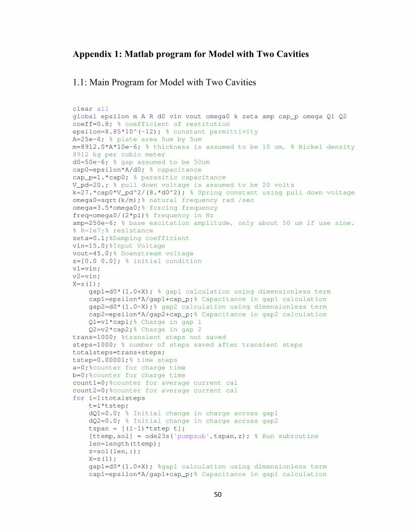
Appendix 1: Matlab program for Model with Two Cavities
1.1: Main Program for Model with Two Cavities
clear all global epsilon m A R d0 vin vout omega0 k zeta amp cap_p omega Q1 Q2 coeff=0.8; % coefficient of restitution epsilon=8.85*10^(-12); % constant permittivity A=25e-6; % plate area 5um by 5um m=8912.0*A*10e-6; % thickness is assumed to be 10 um, % Nickel density 8912 kg per cubic meter d0=50e-6; % gap assumed to be 50um cap0=epsilon*A/d0; % capacitance cap_p=1.*cap0; % parasitic capacitance V_pd=20.; % pull down voltage is assumed to be 20 volts k=27.*cap0*V_pd^2/(8.*d0^2); % Spring constant using pull down voltage omega0=sqrt(k/m);% natural frequency rad /sec omega=3.5*omega0;% forcing frequency freq=omega0/(2*pi)% frequency in Hz amp=250e-6; % base excitation amplitude, only about 50 um if use sine. % R=1e7;% resistance zeta=0.1;%Damping coefficient vin=15.0;%Input Voltage vout=45.0;% Downstream voltage z=[0.0 0.0]; % initial condition v1=vin; v2=vin; X=z(1); gap1=d0*(1.0+X); % gap1 calculation using dimensionless term cap1=epsilon*A/gap1+cap_p;% Capacitance in gap1 calculation gap2=d0*(1.0-X);% gap2 calculation using dimensionless term cap2=epsilon*A/gap2+cap_p;% Capacitance in gap2 calculation Q1=v1*cap1;% Charge in gap 1 Q2=v2*cap2;% Charge in gap 2 trans=1000; %transient steps not saved steps=1000; % number of steps saved after transient steps totalsteps=trans+steps; tstep=0.00001;% time steps a=0;%counter for charge time b=0;%counter for charge time count1=0;%counter for average current cal count2=0;%counter for average current cal for i=1:totalsteps t=i*tstep; dQ1=0.0; % Initial change in charge across gap1 dQ2=0.0; % Initial change in charge across gap2 tspan = [(i-1)*tstep t]; [ttemp,sol] = ode23s('pumpsub',tspan,z); % Run subroutine len=length(ttemp); z=sol(len,:); X=z(1); gap1=d0*(1.0+X); %gap1 calculation using dimensionless term cap1=epsilon*A/gap1+cap_p;% Capacitance in gap1 calculation
51
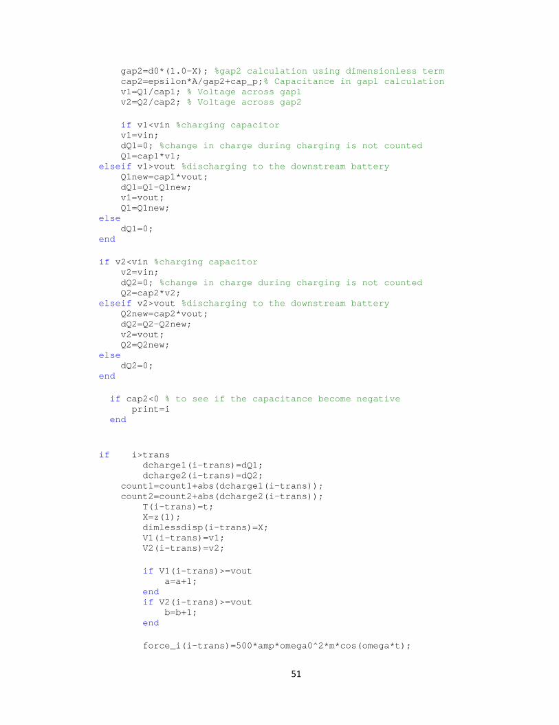
gap2=d0*(1.0-X); %gap2 calculation using dimensionless term cap2=epsilon*A/gap2+cap_p;% Capacitance in gap1 calculation v1=Q1/cap1; % Voltage across gap1 v2=Q2/cap2; % Voltage across gap2 if v1<vin %charging capacitor v1=vin; dQ1=0; %change in charge during charging is not counted Q1=cap1*v1; elseif v1>vout %discharging to the downstream battery Q1new=cap1*vout; dQ1=Q1-Q1new; v1=vout; Q1=Q1new; else dQ1=0; end if v2<vin %charging capacitor v2=vin; dQ2=0; %change in charge during charging is not counted Q2=cap2*v2; elseif v2>vout %discharging to the downstream battery Q2new=cap2*vout; dQ2=Q2-Q2new; v2=vout; Q2=Q2new; else dQ2=0; end if cap2<0 % to see if the capacitance become negative print=i end if i>trans dcharge1(i-trans)=dQ1; dcharge2(i-trans)=dQ2; count1=count1+abs(dcharge1(i-trans)); count2=count2+abs(dcharge2(i-trans)); T(i-trans)=t; X=z(1); dimlessdisp(i-trans)=X; V1(i-trans)=v1; V2(i-trans)=v2; if V1(i-trans)>=vout a=a+1; end if V2(i-trans)>=vout b=b+1; end force_i(i-trans)=500*amp*omega0^2*m*cos(omega*t);
52
end % check if collision has occurred end chargetime=(a+b)* tstep % Calculate charge time Averagecurrent=((count1+count2)/(2*steps*tstep))% Calculate average current subplot(3,1,1); plot(T,dimlessdisp,T,force_i); xlabel('Time(t)-sec','FontSize',10) ylabel('Displacement ','FontSize',10) subplot(3,1,2); plot(T,V1,T,V2); xlabel('Time(t)-sec','FontSize',10) ylabel('Voltage ','FontSize',10) subplot(3,1,3); plot(T,dcharge1,T,dcharge2); xlabel('Time(t)-sec','FontSize',10) ylabel('Change in charge - Coulomb ','FontSize',10) % subplot(4,1,4); plot(T,Q1,T,Q2); % xlabel('Time(t)-sec','FontSize',10) % ylabel('Charge across gaps - Coulomb ','FontSize',10)
1.2: Subroutine Program for Model with Two Cavities
function xdot = pumpsub(t,x); % with two capacitors global epsilon m A R d0 vin vout omega0 k zeta amp cap_p omega Q1 Q2 % Q2=0.;% for single cavity only d1=d0*(1.+x(1)); d2=d0*(1.-x(1)); xdot(1,1)=x(2); k2=1000*k; % stopper spring stiffness is considered to be 1000 times of total stiffness of serpentine spring % force_e=-epsilon*A*(v1^2/(2.0*d1^2)-v2^2/(2.0*d2^2)); force_e=(-Q1^2+Q2^2)/(epsilon*A); force_i=-amp*omega^2*m*cos(omega*t); %bigger transient with sin. if x(1)<-0.8 force_s = (k2/abs(1+x(1)))*abs(-x(1)-0.8); elseif x(1)>0.8 force_s= -(k2/abs(1-x(1)))*abs(x(1)-0.8); else force_s=0.; end xdot(2,1)=-2.0*omega0*zeta*x(2)-omega0^2*x(1)+(force_s+(force_e+force_i)/d0)/m;
53
Appendix 2: Matlab program for Model with Single Cavities
2.1: Main Program for single cavity model
clear all global epsilon m A R d0 vin vout omega0 k zeta amp cap_p omega Q1 Q2 coeff=0.8; % coefficient of restitution epsilon=8.85*10^(-12); % constant permittivity A=25e-6; % plate area 5um by 5um m=8912.0*A*10e-6; % thickness is assumed to be 10 um, % Nickel density 8912 kg per cubic meter d0=50e-6; % gap assumed to be 50um cap0=epsilon*A/d0; % capacitance cap_p=1.*cap0; % parasitic capacitance V_pd=20.; % pull down voltage is assumed to be 20 volts k=27.*cap0*V_pd^2/(8.*d0^2); % Spring constant using pull down voltage omega0=sqrt(k/m);% natural frequency rad /sec omega=3.5*omega0;% forcing frequency freq=omega0/(2*pi)% frequency in Hz amp=250e-6; % base excitation amplitude, only about 50 um if use sine. % R=1e7;% resistance zeta=0.1;%Damping coefficient vin=15.0;%Input Voltage vout=45;% Downstream voltage z=[0.0 0.0]; % initial condition v1=vin; v2=vin; X=z(1); gap1=d0*(1.0+X); % gap1 calculation using dimensionless term cap1=epsilon*A/gap1+cap_p;% Capacitance in gap1 calculation gap2=d0*(1.0-X);% gap2 calculation using dimensionless term cap2=epsilon*A/gap2+cap_p;% Capacitance in gap2 calculation Q1=v1*cap1;% Charge in gap 1 Q2=v2*cap2;% Charge in gap 2 trans=1000; %transient steps not saved steps=1000; % number of steps saved after transient steps totalsteps=trans+steps; tstep=0.000001;% time steps a=0;%counter for charge time b=0;%counter for charge time count1=0;%counter for average current cal count2=0;%counter for average current cal for i=1:totalsteps t=i*tstep; dQ1=0.0; % Initial change in charge across gap1 dQ2=0.0; % Initial change in charge across gap2 tspan = [(i-1)*tstep t]; [ttemp,sol] = ode23s('pumpsub',tspan,z); % Run subroutine len=length(ttemp); z=sol(len,:); X=z(1); vel=z(2); eps=-tstep*vel;
54
if abs(X+0.8)<eps/2 z(1)=-0.8; z(2)=-coeff*vel; end X=z(1); gap1=d0*(1.0+X); %gap1 calculation using dimensionless term cap1=epsilon*A/gap1+cap_p;% Capacitance in gap1 calculation gap2=d0*(1.0-X); %gap2 calculation using dimensionless term cap2=epsilon*A/gap2+cap_p;% Capacitance in gap1 calculation v1=Q1/cap1; % Voltage across gap1 v2=Q2/cap2; % Voltage across gap2 if v1<vin %charging capacitor v1=vin; dQ1=0; %change in charge during charging is not counted Q1=cap1*v1; elseif v1>vout %discharging to the downstream battery Q1new=cap1*vout; dQ1=Q1-Q1new; v1=vout; Q1=Q1new; else dQ1=0; end if v2<vin %charging capacitor v2=vin; dQ2=0; %change in charge during charging is not counted Q2=cap2*v2; elseif v2>vout %discharging to the downstream battery Q2new=cap2*vout; dQ2=Q2-Q2new; v2=vout; Q2=Q2new; else dQ2=0; end if cap2<0 % to see if the capacitance become negative print=i end if i>trans dcharge1(i-trans)=dQ1; dcharge2(i-trans)=dQ2; count1=count1+abs(dcharge1(i-trans)); count2=count2+abs(dcharge2(i-trans)); T(i-trans)=t; X=z(1); dimlessdisp(i-trans)=X; V1(i-trans)=v1; V2(i-trans)=v2; if V1(i-trans)>=45 a=a+1; end
55
if V2(i-trans)>=45 b=b+1; end force_i(i-trans)=50*amp*omega0^2*m*cos(omega*t); end % check if collision has occurred end chargetime=(a+b)* tstep % Calculate charge time Averagecurrent=((count1+count2)/(2*steps*tstep))% Calculate average current subplot(3,1,1); plot(T,dimlessdisp,T,force_i); xlabel('Time(t)-sec','FontSize',10) ylabel('Displacement ','FontSize',10) subplot(3,1,2); plot(T,V1,T,V2); xlabel('Time(t)-sec','FontSize',10) ylabel('Voltage ','FontSize',10) subplot(3,1,3); plot(T,dcharge1,T,dcharge2); xlabel('Time(t)-sec','FontSize',10) ylabel('Change in charge - Coulomb ','FontSize',10) % subplot(4,1,4); plot(T,Q1,T,Q2); % xlabel('Time(t)-sec','FontSize',10) % ylabel('Charge across gaps - Coulomb ','FontSize',10)
2.2: Subroutine Program for single cavity model
function xdot = pumpsub(t,x); % with two capacitors global epsilon m A R d0 vin vout omega0 k zeta amp cap_p omega Q1 Q2 Q2=0.;% for single cavity only d1=d0*(1.+x(1)); d2=d0*(1.-x(1)); cap1=epsilon*A/d1+cap_p; cap2=epsilon*A/d2+cap_p; v1=Q1/cap1; v2=Q2/cap2; xdot(1,1)=x(2); k2=1000*k; % stopper spring stiffness is considered to be 1000 times of total stiffness of serpentine spring % force_e=-epsilon*A*(v1^2/(2.0*d1^2)-v2^2/(2.0*d2^2)); force_e=(-Q1^2+Q2^2)/(epsilon*A); force_i=-amp*omega^2*m*cos(omega*t); %bigger transient with sin. if x(1)<-0.8 force_s = (k2/abs(1+x(1)))*abs(-x(1)-0.8)*d0; % elseif x(1)>0.8 % force_s= -(k2/abs(1-x(1)))*abs(x(1)-0.8); else force_s=0.; end xdot(2,1)=-2.0*omega0*zeta*x(2)-omega0^2*x(1)+(force_s+(force_e+force_i)/d0)/m;