Design and Optimization of a Vortex Particle Separator for a Hot Mix Asphalt Plant

Andrew Hobbs Astec Industries, Chattanooga, TN 37407

Abstract

Particle/gas separation is a necessary step in the production of Hot Mix Asphalt (HMA). Process requirements demand a very specific separation criteria. In addition, the pressure drop associated with the separation stage must be minimized to reduce the static pressure required from the fan. The intent of this study was to design and optimize an inline cyclonic particle separator as the primary collector for a HMA plant. Computation Fluid Dynamics (CFD) methods were used to investigate the effects of the device geometry on particle collection. Parametric studies of the geometry were accomplished using ICEMCFD’s direct CAD interface in SolidWorks. The Reynolds Renormalization Group (RNG) ε−k turbulence model was used to model the swirling flow. Particle tracking was performed to predict collection efficiency using a Discrete Phase Model (DPM). The Haider and Levenspeil modification was made to the DPM to better model non-spherical particles trajectories. Particle-wall interaction was investigated by varying the Coefficient of Restitution. The predicted collection efficiency was compared to a similar CFD analysis of the existing HMA cyclone design and to empirical data. The optimized inline cyclonic separator was shown to accomplish qualitatively better collection efficiency at a fraction of the pressure drop of the existing design.

Introduction Hot mix asphalt (HMA) is the most common road surfacing material used in the United States. Between 450,000,000 and 500,000,000 tons of hot mix asphalt are produced annually in the U.S. alone. HMA is comprised of sand and various sizes of crushed rock, called aggregate, which is mixed together with liquid asphalt cement. The liquid asphalt cement acts as a binder. The mixture is thermoformable and begins to set at temperatures below 300o F.

The modern hot mix asphalt plant is comprised of several components, each of which performs a specific task in the production of the asphalt mixture (see Figure 1). Aggregate is typically stored in large stockpiles outdoors where it is exposed to the weather. Any moisture in the aggregate can cause poor coating, so the aggregate must be dried before the liquid asphalt can be introduced. The aggregate is loaded into feeder bins which meter out the different sized aggregate. The aggregate is then fed into a rotating drum where it is tumbled while being exposed to hot gases from a burner. Once the aggregate is dry, it is mixed with the liquid asphalt cement and stored in an insulated silo until it is loaded into trucks to be taken to the jobsite.

Figure 1. HMA plant component schematic

As aggregate is dried in the drum by the hot gases from the burner, dust from the aggregate is carried away in the exhaust gases. Particulate in the exhaust gas stream must be removed to meet current environmental emission standards, making the separation of particulate from the exhaust gases a necessary step in the production of hot mix asphalt. In addition, HMA mix design requires a certain percentage of fine material or fines to be included in the mix. The fine material to be included in the mix is made up of dust and sand larger than 150 µm. A certain quantity of this sized material is needed to give the asphalt mix the desired properties. Any of this fine material entrained in the gas stream must be separated and returned to the mix.

Cleaning and separating is traditionally accomplished in two stages: an inertially driven primary collector and a fabric filter-based secondary collector. Nominally, the primary collector removes all particles larger than approximately 150 µm and passes all particles smaller than 150 µm to the secondary collector (J.D. Brock, 1999). The larger particles are added to the HMA mix and the smaller particles remain in the gas stream. Traditionally, a cyclone is used as the primary collector.

The secondary collector is typically a fabric filtration system called a baghouse. Particulate accumulates on the fabric media forming a thin layer of dust called a “cake.” It is the cake which actually accomplishes the filtration of the smallest particles. Large particles make the cake more porous allowing smaller particles to pass through unfiltered. Large particles can also cause abrasion, leading to shortened bag life. Hence it is necessary for the primary collector to remove the larger particles but pass the smaller particles (M. Swanson, 1999).

The limiting factor of the filtration system is the fan horsepower required to pull air through the pre-collector and the filter media. Because of this, minimizing the pressure drop associated with the overall filtration process is a key design consideration. However, most cyclones are typically designed for maximum efficiency with less concern for pressure drop. The design requirements of the primary collector in a HMA plant are unique. It must be able to remove large particles (greater than 100 µm) very efficiently while passing the majority of the small particles at a relatively low pressure drop for a nominal flow rate of 67,000 ft3/min. Cyclonic separators are a common method of particle removal because they have no moving parts and can withstand high operational temperatures with relatively inexpensive maintenance costs. However, due to the unique combination of conditions and the performance requirements of a HMA plant, a traditional

reverse flow cyclone is not optimally suited as a primary collector. The high flow rates and relatively large cut size require such a cyclone to be quite large. In addition the pressure drop for such a device places a large drain on the available power of the system fan. Cyclone technology is over a hundred years old, and while the precise nature of the flow within the cyclone is not fully known, there has been much empirical and theoretical study which has provided a general understanding of characteristic performance. Much of the development in cyclone design has come as a result of trial and error experimentation. While this type of experimentation yields the most accurate results, it is time consuming and costly. Empirical and semi-empirical models of cyclone behavior have been developed, but their usefulness if often very limited if the geometry does not sufficiently match the model. The use of computational fluid dynamics (CFD) software to predict the performance of a cyclone has been shown to be more accurate than empirical models, and the analysis can be performed in shorter time and with less cost than physical experimentation (Griffiths and Boysan, 1996; Ma et al., 2000).

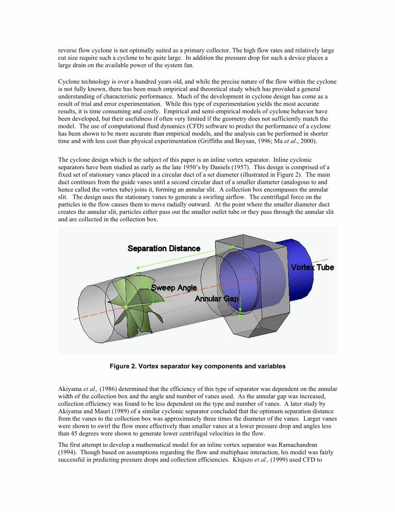
The cyclone design which is the subject of this paper is an inline vortex separator. Inline cyclonic separators have been studied as early as the late 1950’s by Daniels (1957). This design is comprised of a fixed set of stationary vanes placed in a circular duct of a set diameter (illustrated in Figure 2). The main duct continues from the guide vanes until a second circular duct of a smaller diameter (analogous to and hence called the vortex tube) joins it, forming an annular slit. A collection box encompasses the annular slit. The design uses the stationary vanes to generate a swirling airflow. The centrifugal force on the particles in the flow causes them to move radially outward. At the point where the smaller diameter duct creates the annular slit, particles either pass out the smaller outlet tube or they pass through the annular slit and are collected in the collection box.

Figure 2. Vortex separator key components and variables

Akiyama et al., (1986) determined that the efficiency of this type of separator was dependent on the annular width of the collection box and the angle and number of vanes used. As the annular gap was increased, collection efficiency was found to be less dependent on the type and number of vanes. A later study by Akiyama and Mauri (1989) of a similar cyclonic separator concluded that the optimum separation distance from the vanes to the collection box was approximately three times the diameter of the vanes. Larger vanes were shown to swirl the flow more effectively than smaller vanes at a lower pressure drop and angles less than 45 degrees were shown to generate lower centrifugal velocities in the flow.

The first attempt to develop a mathematical model for an inline vortex separator was Ramachandran (1994). Though based on assumptions regarding the flow and multiphase interaction, his model was fairly successful in predicting pressure drops and collection efficiencies. Klujszo et al., (1999) used CFD to

further investigate the effects key design parameters of the inline. The variables investigated by Klujszo are the overall diameter, blade geometry, separation distance, collection gap size and airflow velocity. These variables were tested using CFD and verified with physical models. Klujszo concluded that the mechanism for separation of the investigated design offered reasonable efficiency at a lower pressure drop than other available methods of separation. He also concluded that increasing the number of guide vanes increases the pressure drop. He determined that there should be no gaps in projected area of the blades. To prevent detrimental low pressure regions he added front and rear cones on the vane hub. Progressively angled vanes (curved) were shown to offer a lower pressure drop than straight vanes. Klujszo determined that an optimum collection distance and gap distance could be found to maximize efficiency. The physical simulations validated the CFD results.

The lower pressure drop and simplicity of the device proposed by Klujzso make it an attractive choice for a pre-collector in a HMA plant. A similar device could be incorporated into existing ductwork making integration very simple. However, the model tested by Klujzso was quite small (51.8mm diameter) and could only handle very small airflows (velocities in the range of 4.2 to 6.1 m/s). The nominal airflow for an HMA plant is 67,000 ft3/min. The intent of this study is to adapt this design for the operating conditions and design specifications of an HMA plant using CFD. The following chapters will describe the procedure implemented in this study, results of the CFD analysis, and finally, conclusions drawn from the results.

Procedure The laws which govern the flow of fluid can be mathematically described in a set of equations known as the Navier-Stokes equations. The Navier-Stokes equations are coupled, non-linear, partial differential equations which describe the mass and momentum conservation of fluids. Because of the complexity of these equations, finding an exact solution for them is often impossible unless many simplifying assumptions are made.

Numerical methods offer a means of approximating the solution of the Navier-Stokes equations. However, the large number of calculations required to approximate the solution of more complex problems necessitates the use of computers. The increasing computational speed of modern computers continues to make more and more types of fluid simulations possible. The numerical studies discussed in this paper were calculated using the commercial CFD code Fluent 6.0.

The fluid domain was described by constructing a solid model of the geometry in the solid modeling software package SolidWorks. This volume was then meshed with an unstructured tetrahedral scheme using ICEMCFD’s tetrahedral meshing module, and the resulting mesh was imported into Fluent’s solver. Boundary conditions were specified, and the solution was run until convergence criteria was met.

As the effects of the geometry are coupled to the performance of the device, it is difficult to isolate a single parameter for investigation. To simplify analysis, first, only the vane geometry was investigated by making key construction dimensions parametric. An optimum geometry was selected by the condition of maximum tangential velocity generated at the wall excluding the boundary layer with the minimum pressure drop. Once a particular vane geometry was chosen, other variables were investigated keeping the vane geometry constant.

The variables investigated in this study were vane design (including overall angle, sweep angle, and departure angle), separation distance, annular gap distance, axial gap distance, and vortex tube shape shown in Figure 2 (blue). For each geometrical variation the following procedure was completed: (1) the specified geometry was constructed or modified, (2) a new mesh was generated for each variation, (3) a solution was run and allowed to converge, (4) the mesh was then refined by gradients to ensure mesh independence and the solution was iterated until convergence was again met, and finally, (5) the results were recorded and tabulated.

Turbulence Model A turbulent flow is characterized by fluctuations in the velocity field. These fluctuations can be very small in scale and potentially high in frequency. To explicitly account for these fluctuations in the Navier-Stokes equations, a method called direct numerical simulation (DNS) must be used. The turbulent fluctuations are caused by flow eddies with a range of length and time scales. The length scale is a physical quantity which relates to the size of the large eddies. For fully developed pipe flow the length scale can be described as l = 0.07D, where D is the pipe diameter. The large scales are measured by the characteristic length of the mean flow and the small scales as the dissipation of kinetic energy. The ratio of large to small scales is proportional to Ret

3/4. In order to accurately simulate all scales of eddies, the mesh would need to be proportional to Ret

9/4. This is computationally beyond reach for the large 3-D geometries of interest in this study.

Because an exact solution is impossible, the instantaneous equations are time averaged to produce a simpler set of equations. This technique is called Reynolds Average Navier-Stokes (RANS). RANS decomposes the exact solution of the Navier-Stokes equations into a mean and fluctuating component. Details of this method are available in literature.

The accuracy of various turbulence models has been investigated for many flow conditions. The models which have been used for cyclone modeling, which involve strong swirling flows, have been the Reynolds stress model (RSM) and the k-ε models (Boysan et al., 1982; Griffiths and Boysan, 1996; Ma et al., 2000). While the ε−k model is a very robust and widely applicable model, it was shown to be less accurate for swirling flow due to the isotropic turbulent viscosity assumption (Boysan et al., 1982). The RSM model has been shown to be more accurate for swirling flow, but it is considerably more computationally intensive (Ma et al., 2000).

A variation of the ε−k model called the Renormalization group method (RNG) was developed to better account for differing flow conditions. The RNG based ε−k model provides the accuracy of the RSM model and the simplicity of the standard ε−k model. The key difference between the standard ε−k and the RNG model is that in the formulation of the RNG model, the calculation of the turbulent viscosity from the solution of an ordinary differential equation takes in to account the effects of rotation and adds an additional term in the dissipation rate transport equation (Griffith and Boysan, 1996).

Fluent 6 offers a further modification of RNG ε−k model to better account for swirling flow. The equation for the turbulent viscosity is modified to include the effects of swirl.

Ω=

εαµµ kf stt ,,0 (14)

where 0tµ is the turbulent viscosity calculated without the swirl modification, Ω is a characteristic swirl

number determined internally in Fluent, and sα is a swirl constant which assumes a default value of 0.05 for mildly swirling flow conditions but can be set higher for strongly swirling flow.

Simulation Parameters The RNG based k-ε model was chosen to model turbulence. The vortex separator was considered to be isolated from the total system. Boundary conditions were chosen to best represent standard operating conditions. The energy equation was selected to account for the high temperature, which was set at 270oF to simulate exhaust gases from the drum. The fluid [air] was assigned the ideal gas law to model the change in density due to the temperature. Pressure was assumed to be atmospheric for the inlet. The gravitational force was set to 32.2ft/s2 in the negative y direction.

To better simulate operational conditions, a velocity boundary condition was set at the outlet rather than the inlet because the fan is pulling rather than blowing air through the system. The inlet was assigned a pressure inlet boundary condition with a gage pressure of 0 inches of water. Turbulent intensity and hydraulic diameters for the inlet and outlet were calculated for the nominal flowrate, and the temperature was set to be constant. The solution was initialized from the outlet velocity conditions and allowed to converge.

Particle Tracking Once a converged solution was obtained for the flow field, the collection efficiency of the design was determined by releasing particles and tracking their trajectories. The Discrete Phase Model (DPM) in Fluent can be used to model bubbles, droplets, or inert particles. The fluid and particle phases can be either coupled or de-coupled based conditions in the flow field. De-coupling the phases, called one-way coupling, assumes that the particle trajectories are determined by the flow field but do not alter the flow as they pass nor do particles interact with each other. These assumptions are desirable because they greatly reduce computation time and are valid if two specific criteria are met. Lun and Bent (1994) concluded that for particle volume fractions less than 10% the dominant mechanism of momentum transfer is the kinetic mode rather than collision with other particles. Hence, the first criteria to validate one-way coupling is that the particle volume fraction must be less than 10% of the fluid volume. Based on nominal HMA plant operating conditions used in this study, a dust volume fraction can be calculated to be less than 0.01%. The second criteria is that the size of the largest particle diameter must be less than the Kolmogorov length scale (the length scale of the smallest turbulent eddies). Studies such as Goubesbet and Berlemont (1999) suggest that particles with diameters smaller than the Kolmogorov scale have negligible influence on local turbulence. The Kolmogorov length scale is given by equation (18).

( ) 413

ενη = (18)

where ν is the kinematic viscosity and ε is the turbulent dissipation rate. A representative value obtained from the CFD results give a Kolmogorov scale of 6.364 X10-4m. The largest particle diameter used in the study was 2.5 X 10-4m. This is smaller but on the same order of the Kolmogorov scale. While the largest particle diameter is of the same order of magnitude of the Kolmogorov scale, one-way coupling was determined to be a valid assumption given the low volume fraction of particles in the system (< 0.01%). One-way coupling also assumes that particles have no interaction with other particles. The particles were specified as inert, meaning that no chemical reactions or phase change were considered. Fluent predicts particle trajectories by integrating the force balance on the particle in a Lagrangian reference frame.

( ) ( )p

ppdrag

p guufdt

duρρρ −

+−= (19)

where dragf is the drag force give by

24Re18

2pD

ppdrag

Cd

fρ

µ= (20)

and particle Reynolds number: µ

ρ uud ppp

−=Re (21)

and u, ρ, are the fluid velocity (or mean velocity for turbulent flow) and fluid density. Particle properties are shown as up, ρp, dp, for particle velocity, density, and diameter, respectively. Fluent allows stochastic particle tracking method called the Discrete Random Walk (DRW) to add in the effect of turbulent fluctuations on particle trajectories. To speed analysis time, most preliminary dimensional investigations involving particle tracking were performed without the DRW model activated, meaning particle trajectories were computed using the mean component of the velocity only. The DRW model was used with the final design iterations to verify the model and previous results. The addition of the DRW model did not alter collection efficiencies significantly. The trajectory equations are solved through a stepwise integration by discrete time steps using a trapezoidal integration scheme. Boundary conditions are set to consider the DPM. If a particle encounters a wall it can either be reflected in a collision, or it can be trapped. Reflective boundaries can be assigned a coefficient of restitution (CoR) which determines the nature of the reflection, either perfectly elastic (CoR = 1) or perfectly plastic (CoR = 0) or any where in between. Non-wall boundary conditions such as inlets and outlets can be assigned as interfaces which allow particles to escape or which trap particles. In this analysis particles were released from the inlet face. The outlet was set to allow particles to escape while the faces in the collection box were set to trap particles. All other surfaces were set to reflect. In this way, the collection efficiency could be determined by calculating the percentage of particles which were trapped. To investigate the effect of the CoR, values of 1, 0.8, 0.6, and 0.4 were used for the CoR on all reflecting boundaries for the final design iteration. An investigation of all available methods of non-spherical particle drag calculations was performed for 1900 data points for various shaped particles for a range of particle Reynolds numbers (R. P. Chhabra, et al., 1998). Available methods were compared for error and ranges of applicability. One method investigated was the Haider and Levenspeil model. Haider and Levenspiel is a semi-empirical model which expresses the particle drag as a function of the particle shape factor. The shape factor φ, is defined as the ratio of the surface area of a same volume spheres, Ss, to the actual surface area of the particles, s. The results of Chhabra, et al. indicate that Haider and Levenspiel satisfactorily predicted drag for particles with values of φ > 0.67. Fluent incorporates the Haider and Levenspiel model as an option in the DPM for modeling non-spherical particles.

sSs

=φ (22)

A sphere has a shape factor of 1. Smaller values of φ indicate less spherity. The Haider and Levenspeil modification is valid for the particle Reynolds number less than 2.6 X105. The maximum particle Reynolds number observed from the particle tracking studies was on the order of 500. The drag coefficient CD from equation (20) is defined according to the Haider and Levenspiel model as the following equations:

( )p

pbp

pD b

bbC

ReRe

Re1Re24

4

31

2

+

+++= (23)

and b1=exp(2.3288 – 6.4581φ + 2.4486φ2 b2= 0.0964 + 1.5565φ b3= exp(4.905 – 13.8944φ + 18.4222φ2 –10.2599φ3) b4= exp(1.4681 + 12.258φ - 20.7322φ2 + 15.8855φ3) where φ is the shape factor defined in equation (22)

The material of the particles was defined as limestone (density = 135lb/ft3, or 2164.5 kg/m3), a common aggregate used in the production of asphalt. Limestone (calcium carbonate) particles are generally cubic in shape, so the shape factor modification for non-spherical particles was set to 0.8. Injections were defined for particle diameters ranging from 250 µm (60 mesh per inch) to 25 µm (500 mesh per inch). Each size was injected separately from the inlet face, and the resultant fates were recorded.

Horizontal Cyclone The analysis of the horizontal cyclone design was performed in much the same way as described for the vortex separator. The geometry was constructed and a mesh generated. The mesh was imported into Fluent and the nominal flow rate and operating conditions were set as with the vortex separator. The flow field was solved, and particle tracking studies were performed. Identical sets of particles were released from the inlet of the horizontal cyclone as were the vortex separator. Particle which passed through the outlet were set to have escaped, and particles which impacted the hopper were set to have been trapped. The same settings for non-spherical particles and turbulent fluctuations were used as with the analysis of the vortex separator.

Analysis Results & Discussion A primary diameter was chosen to be 5.167ft to give 3400 fpm (17.45 m/s) for 67,000 ft3/min. Preliminary testing showed that the blade design was the driving factor in changing the flow. It was therefore decided that the blade and hub design be investigated first.

Blade Geometry

The blade geometry was made parametric and solutions were run in order to correlate flow characteristics to the blade geometry. The number of blades was chosen to be eight positioned about at six inch diameter hub. The axial blade length was set at two feet. The geometric variables used were the sweep angle and departure angle (figure 3 and figure 4). The front and rear cone, as well as the axial blade length, were kept constant.

Figure 3. Front elevation of blade and hub geometry showing sweep angle

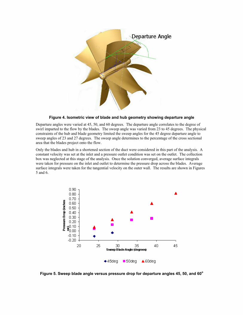
Figure 4. Isometric view of blade and hub geometry showing departure angle

Departure angles were varied at 45, 50, and 60 degrees. The departure angle correlates to the degree of swirl imparted to the flow by the blades. The sweep angle was varied from 23 to 45 degrees. The physical constraints of the hub and blade geometry limited the sweep angles for the 45 degree departure angle to sweep angles of 23 and 27 degrees. The sweep angle determines to the percentage of the cross sectional area that the blades project onto the flow.

Only the blades and hub in a shortened section of the duct were considered in this part of the analysis. A constant velocity was set at the inlet and a pressure outlet condition was set on the outlet. The collection box was neglected at this stage of the analysis. Once the solution converged, average surface integrals were taken for pressure on the inlet and outlet to determine the pressure drop across the blades. Average surface integrals were taken for the tangential velocity on the outer wall. The results are shown in Figures 5 and 6.

Figure 5. Sweep blade angle versus pressure drop for departure angles 45, 50, and 60o

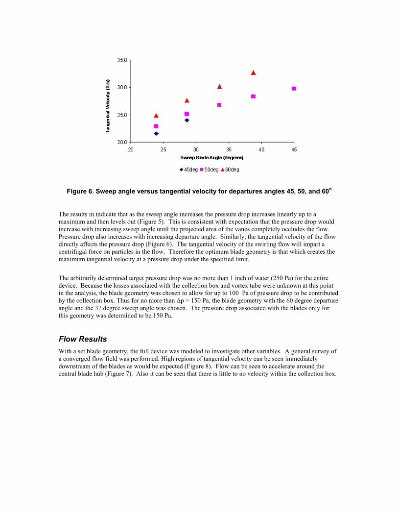
Figure 6. Sweep angle versus tangential velocity for departures angles 45, 50, and 60o

The results in indicate that as the sweep angle increases the pressure drop increases linearly up to a maximum and then levels out (Figure 5). This is consistent with expectation that the pressure drop would increase with increasing sweep angle until the projected area of the vanes completely occludes the flow. Pressure drop also increases with increasing departure angle. Similarly, the tangential velocity of the flow directly affects the pressure drop (Figure 6). The tangential velocity of the swirling flow will impart a centrifugal force on particles in the flow. Therefore the optimum blade geometry is that which creates the maximum tangential velocity at a pressure drop under the specified limit.

The arbitrarily determined target pressure drop was no more than 1 inch of water (250 Pa) for the entire device. Because the losses associated with the collection box and vortex tube were unknown at this point in the analysis, the blade geometry was chosen to allow for up to 100 Pa of pressure drop to be contributed by the collection box. Thus for no more than ∆p = 150 Pa, the blade geometry with the 60 degree departure angle and the 37 degree sweep angle was chosen. The pressure drop associated with the blades only for this geometry was determined to be 150 Pa.

Flow Results With a set blade geometry, the full device was modeled to investigate other variables. A general survey of a converged flow field was performed. High regions of tangential velocity can be seen immediately downstream of the blades as would be expected (Figure 8). Flow can be seen to accelerate around the central blade hub (Figure 7). Also it can be seen that there is little to no velocity within the collection box.

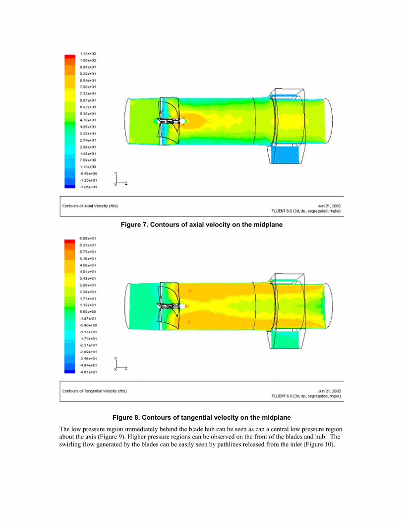
Figure 7. Contours of axial velocity on the midplane

Figure 8. Contours of tangential velocity on the midplane

The low pressure region immediately behind the blade hub can be seen as can a central low pressure region about the axis (Figure 9). Higher pressure regions can be observed on the front of the blades and hub. The swirling flow generated by the blades can be easily seen by pathlines released from the inlet (Figure 10).

Figure 9. Contours of static pressure in inches of water on the midplane and blades

Figure 10. Pathlines release from the inlet colored by velocity magnitude

To gain an understanding of the general behavior of particles in the flow field, single particle were injected into the flow from the inlet. The injection point was varied radially. Two particle sizes were chosen, 150 and 75 µm diameters. The trend indicates that, in general, the larger diameter particles (shown in red) take

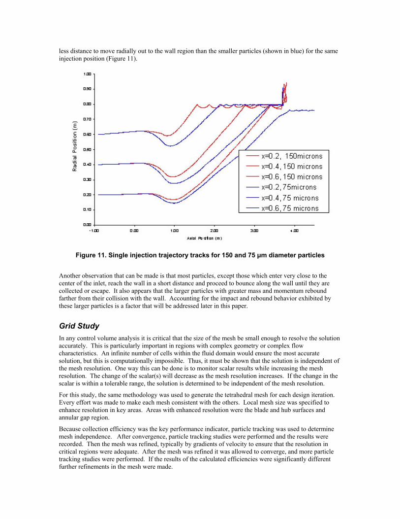
less distance to move radially out to the wall region than the smaller particles (shown in blue) for the same injection position (Figure 11).

Figure 11. Single injection trajectory tracks for 150 and 75 µm diameter particles

Another observation that can be made is that most particles, except those which enter very close to the center of the inlet, reach the wall in a short distance and proceed to bounce along the wall until they are collected or escape. It also appears that the larger particles with greater mass and momentum rebound farther from their collision with the wall. Accounting for the impact and rebound behavior exhibited by these larger particles is a factor that will be addressed later in this paper.

Grid Study In any control volume analysis it is critical that the size of the mesh be small enough to resolve the solution accurately. This is particularly important in regions with complex geometry or complex flow characteristics. An infinite number of cells within the fluid domain would ensure the most accurate solution, but this is computationally impossible. Thus, it must be shown that the solution is independent of the mesh resolution. One way this can be done is to monitor scalar results while increasing the mesh resolution. The change of the scalar(s) will decrease as the mesh resolution increases. If the change in the scalar is within a tolerable range, the solution is determined to be independent of the mesh resolution.

For this study, the same methodology was used to generate the tetrahedral mesh for each design iteration. Every effort was made to make each mesh consistent with the others. Local mesh size was specified to enhance resolution in key areas. Areas with enhanced resolution were the blade and hub surfaces and annular gap region.

Because collection efficiency was the key performance indicator, particle tracking was used to determine mesh independence. After convergence, particle tracking studies were performed and the results were recorded. Then the mesh was refined, typically by gradients of velocity to ensure that the resolution in critical regions were adequate. After the mesh was refined it was allowed to converge, and more particle tracking studies were performed. If the results of the calculated efficiencies were significantly different further refinements in the mesh were made.

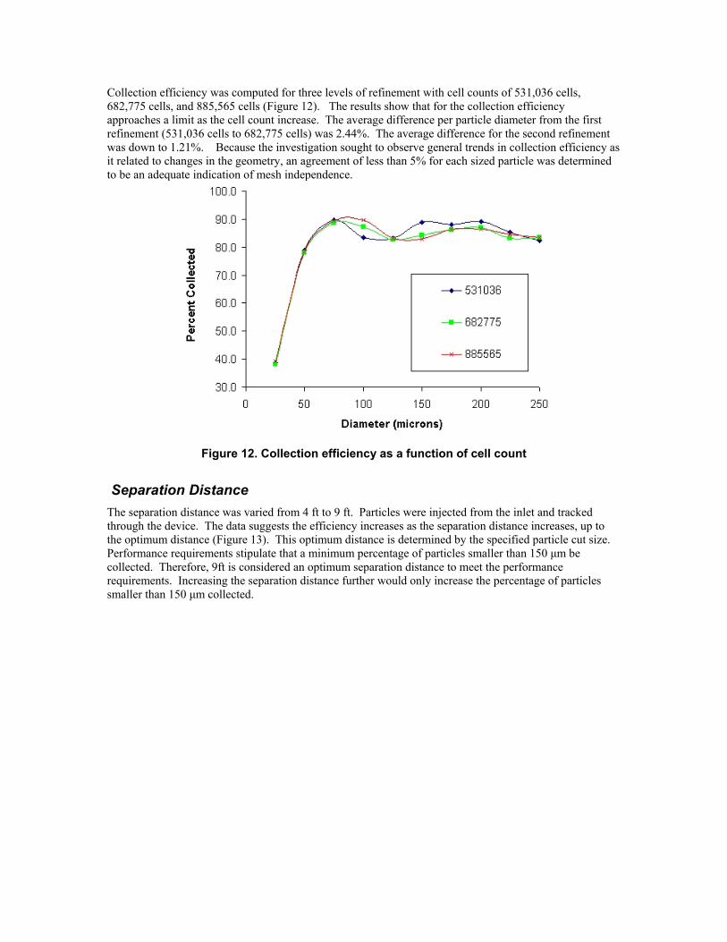
Collection efficiency was computed for three levels of refinement with cell counts of 531,036 cells, 682,775 cells, and 885,565 cells (Figure 12). The results show that for the collection efficiency approaches a limit as the cell count increase. The average difference per particle diameter from the first refinement (531,036 cells to 682,775 cells) was 2.44%. The average difference for the second refinement was down to 1.21%. Because the investigation sought to observe general trends in collection efficiency as it related to changes in the geometry, an agreement of less than 5% for each sized particle was determined to be an adequate indication of mesh independence.

Figure 12. Collection efficiency as a function of cell count

Separation Distance The separation distance was varied from 4 ft to 9 ft. Particles were injected from the inlet and tracked through the device. The data suggests the efficiency increases as the separation distance increases, up to the optimum distance (Figure 13). This optimum distance is determined by the specified particle cut size. Performance requirements stipulate that a minimum percentage of particles smaller than 150 µm be collected. Therefore, 9ft is considered an optimum separation distance to meet the performance requirements. Increasing the separation distance further would only increase the percentage of particles smaller than 150 µm collected.

Figure 13. Collection efficiency as a function of separation distance

Annular Gap Distance The annular gap distance was varied from 1.5 inches (38.1mm) to 3 inches (76.2mm) holding the diameter of the main duct constant. A similar analysis was performed as with the separation distance. Particles were injected from the inlet, and their fates were tracked and recorded. The results show that, in general, as the collection gap increased, efficiency also increased (Figure 14). This is reasonable as the projected escape area increases with the growing gap. However, because the main duct diameter was held constant, change of the annular gap required the diameter of the vortex tube to decrease. This reduced the projected outlet area, which caused the pressure drop to increase.

Figure 14. Particle efficiency as a function of annular gap distance

An alternative method of increasing the annular gap without affecting the outlet area is to flange the main duct diameter near the inlet to the collection box. This flange is a conic section attached to the collection box (Figure 15). A side elevation details the location of the annular gap (Figure 16). The axial length of the flange section is 2 ft with a radial increase of 2 inches over the main duct diameter of 5ft 2 inches. This provides an effective annular gap of 4 inches while maintaining the outlet diameter of 5ft.

Figure 15. Device showing flange section (in green) next to collection box

Figure 16. Side elevation detail of flange section showing annular gap

The results show that the flange section provides higher collection efficiencies for particles larger than 100 µm in diameter and poorer efficiency for particles smaller than 100 µm in diameter than the non-flanged geometry (Figure 17). This difference in the collection of larger particles can be attributed to the larger annular gap afforded by the flange which allows more particles to be separated and the increase in radial distance which encourage larger particles which are rebounding from the wall to be collected. The decrease in the collection efficiency of smaller particles observed in the flanged geometry can be attributed to the subtle change in pressure and velocity fields in the region of the annular gap. The following four

figures display contours of axial velocity and static pressure on the midplane in the annular gap region for the non-flanged and flanged geometry, respectively (Figures 18 through 21).

Figure 17. Effect of flange section on collection efficiency

Figure 18. Contours of axial velocity on midplane for non-flanged geometry

Figure 19. Contours of axial velocity on the midplane for flanged geometry

Figure 20. Contours of static pressure on the midplane for the non-flanged geometry

Figure 21. Contours of static pressure on the midplane for the flanged geometry Comparison of the pressure and velocity contours show that the flanged geometry provides a slightly higher pressure and lower axial velocity in the region of the annular gap than the non-flanged geometry. This Bernoulli effect causes smaller particles with less momentum to avoid this higher pressure and lower axial velocity region in the flanged geometry and are consequently not collected. Larger particles with greater momentum are less affected.

Axial Gap Distance A variable which was not investigated by Klujzso (1999) was the distance from the vortex tube to the front of the collection box called the axial gap in this paper (Figure 22). This distance is perpendicular to the collection gap. The distance of this axial gap was varied to investigate the effect on collection effeciency. The dimensions assigned to this variable were as follows: 0 axial gap indicates that the vortex tube was even with the collection box, 1 to 3 inches axial gaps were varying degrees of distance that the vortex tube was backed away from the front face of the collection box leaving the gap, and -0.5 inch axial gap refers to the vortex tube moving the opposite direction toward the blades. In general, for smaller particles sizes, collection efficiency was shown to improve with increasing axial gap with the exception of the 1in axial gap, but no clear trend can be observed for particles larger than 100 µm in diameter (Figure 23). Because the axial gap variance showed no clear increase in efficiency for larger particles, the geometry was set with no axial gap.

Figure 22. Side elevation showing axial gap detail

Figure 23. Collection efficiency as a function of axial gap distance

Discrete Phase Modifications With the geometric dimension established, the effects of turbulence were included into the particle tracking. The DRW model was activated to include the turbulent fluctuations in the particle trajectory calculations. Results are shown for the collection efficiency of the device for particle trajectories calculated with and without the DRW model (Figure 24). The turbulent fluctuations seem to have little to no effect on particles larger than 150 µm in diameter. The effect on particles smaller than 150 µm in diameter is an average of 25.3% increased collection efficiency for the DRW model.

Figure 24. Final design collection efficiency showing DRW model and mean velocity

The final variable investigated was the coefficient of restitution. All particle trajectories calculated up to this point had assumed a perfectly elastic collision (CoR = 1) with wall boundaries. Because many particles appear to reach the tube wall before the collection box, the nature of the collision(s) with the tube wall affects the particle trajectories and also the resulting collection efficiency of the device. To determine the effect of the particle-wall collisions, the CoR was varied from 0.4 to 1. The results indicate three distinct characteristic regions which depend on particle diameter (Figure 25). The first characteristic behavior is exhibited by particles smaller than 75 µm. These particles are little affected by changes in the value of the CoR. This is largely due to the fact that most of these particles do not interact with the wall.

Figure 25. Collection efficiency for varied coefficient of restitution

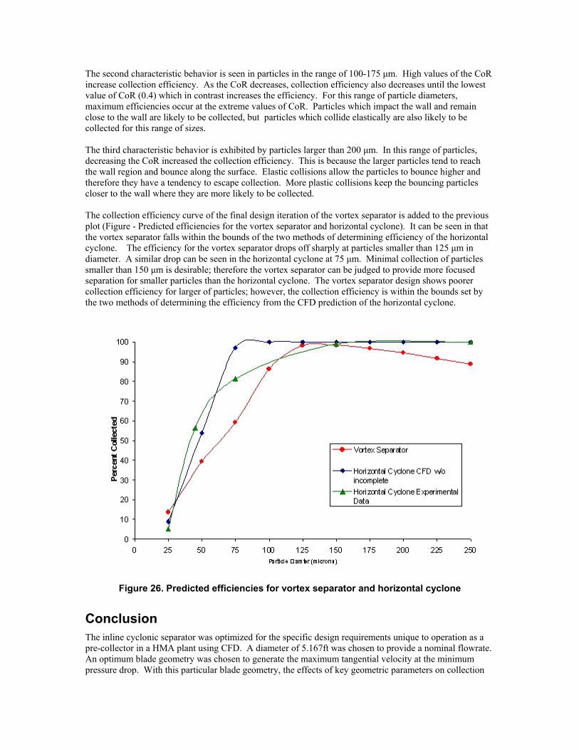
The second characteristic behavior is seen in particles in the range of 100-175 µm. High values of the CoR increase collection efficiency. As the CoR decreases, collection efficiency also decreases until the lowest value of CoR (0.4) which in contrast increases the efficiency. For this range of particle diameters, maximum efficiencies occur at the extreme values of CoR. Particles which impact the wall and remain close to the wall are likely to be collected, but particles which collide elastically are also likely to be collected for this range of sizes. The third characteristic behavior is exhibited by particles larger than 200 µm. In this range of particles, decreasing the CoR increased the collection efficiency. This is because the larger particles tend to reach the wall region and bounce along the surface. Elastic collisions allow the particles to bounce higher and therefore they have a tendency to escape collection. More plastic collisions keep the bouncing particles closer to the wall where they are more likely to be collected. The collection efficiency curve of the final design iteration of the vortex separator is added to the previous plot (Figure - Predicted efficiencies for the vortex separator and horizontal cyclone). It can be seen in that the vortex separator falls within the bounds of the two methods of determining efficiency of the horizontal cyclone. The efficiency for the vortex separator drops off sharply at particles smaller than 125 µm in diameter. A similar drop can be seen in the horizontal cyclone at 75 µm. Minimal collection of particles smaller than 150 µm is desirable; therefore the vortex separator can be judged to provide more focused separation for smaller particles than the horizontal cyclone. The vortex separator design shows poorer collection efficiency for larger of particles; however, the collection efficiency is within the bounds set by the two methods of determining the efficiency from the CFD prediction of the horizontal cyclone.

Figure 26. Predicted efficiencies for vortex separator and horizontal cyclone

Conclusion The inline cyclonic separator was optimized for the specific design requirements unique to operation as a pre-collector in a HMA plant using CFD. A diameter of 5.167ft was chosen to provide a nominal flowrate. An optimum blade geometry was chosen to generate the maximum tangential velocity at the minimum pressure drop. With this particular blade geometry, the effects of key geometric parameters on collection

efficiency were investigated. These parameters were the separation distance, annular gap, axial gap, and the effects of a flanged duct. Optimum dimensions were determined for each of these parameters to meet the original design specifications: maximum efficiency for particles greater than 150 µm in diameter and minimum efficiency for particles smaller than 150 µm in diameter. The optimum separation distance was determined to be 9 ft. A flanged transition into the collection box was shown to improve collection efficiency by increasing the annular gap to 4 inches without restricting the projected area of the outlet. This flanged section was shown to increase the efficiency of particles larger than 100 µm in diameter. No discernable trend was observed for variance of the axial gap, and therefore it was not included in the final design iteration. Particle trajectory tracking was performed for a range of sizes of limestone particles for each design iteration using the Haider and Levenspiel model for non-spherical particles. The collection efficiency was determined by the percentage of particles that were trapped in the collection box. The system pressure drop was found to be 0.52 inches of water (130 Pa), well below the original design specification of 1 inch of water. The effects of particle-wall impacts were investigated by varying the coefficient of restitution (CoR). Low values of CoR indicating more plastic collisions were shown to increase the collection efficiency for larger particles. Higher values of the CoR indicating more elastic collisions were shown to increase collection efficiency for particles in the 100-150 µm diameter range while decreasing efficiency for the largest of particle sizes. Because the Haider and Levenspeil model does not consider particle orientation and the orientation of a non-spherical particle would certainly affect particle-wall collisions, the varied collection efficiencies for different values of CoR provide a range of possible particle-wall interactions and the resulting collection efficiencies. Given the limitations of the model, the effects of these varied particle-wall interactions may be the best possible way to predict the effects of irregular shaped particle-wall collisions. It is probable that experimentally obtained collection efficiencies for irregular shaped dust particles may be represented by an average of the collection efficiency curves representing different values of the CoR. The existing horizontal cyclone currently used in typical HMA plants was modeled, and the flow field was calculated. Particle tracking studies were performed using the same criteria established for vortex separator. Predicted collection efficiencies were shown to resemble experimental data taken from collected dust samples. The predicted pressure drop across the device was approximately 10% lower than the experimentally measured value. In conclusion, the predicted performance of the final design iteration meets the operational requirements of a HMA plant primary collector. Collection efficiencies were shown to be comparable to that of the existing horizontal cyclone design. The pressure drop across the device was shown to be approximately 1/6 that of the horizontal cyclone design currently in use. The predicted collection efficiency provides satisfactory performance over a range of values for variables including the shape factor and the CoR. The use of these two variables make the particle trajectory calculations more representative of real world operating conditions.

References 1. Akiyama, T., Marul, T., and Kono, M., (1986) Experimental investigation on dust 2. collection efficiency of straight-through cyclones with air suction by means of secondary

rotational air charge. Industrial and Engineering Chemistry Process Design and Development 25, 914-918.

3. Akiyama, T., and Marui, T., (1989) Dust collection efficiency of a straight-through cyclone – effects of duct length, guide vanes and nozzle angle for secondary rotational air flow. Powder Technology 58, 181-185.

4. Brock, J.D. (1997) Baghouse fines, Technical Paper T-121. Astec Industries, Chattanooga, TN.

5. Chhabra, R.P., Agarwal, L., and Sinha, N.K. (1998) Drag on non-spherical particles: an evaluation of available methods. Powder Technology 101, 288-295

6. Fluent 6.0 Users Guide

7. Gouesbet, G., Berlemont,A. (1999) Eulerian and Lagrangian approaches for predicting the behaviour of discrete particles in turbulent flows. Progr. Energy Combust. Sci. 25, 133-159

8. Griffith, W.D. and Boysan, F. (1996) Computational fluid dynamics (CFD) and empirical modeling of the performance of a number of cyclone samplers. J. Aerosol Sci. 27, 281-304.

9. Klujszo, L.A.C., Songfack, P.K., Rafaelof, M., and Rajamani, R.K. (1999) Design of a stationary guide vane swirl air cleaner. Mineral Engineering 12, 1375-1392

10. Lun, C.K.K. and Bent, A. A. (1994) Numerical simulation of inelastic frictional spheres in a simple shear flow. J. Fluid Mech. 258, 335-353

11. Ma, L. Ingham, D.B. and Wen, X. (1999) Numerical modeling of the fluid and particle penetration through small sampling cyclones. J. Aerosol Sci. 31,1097-1119

Ramachandran, G., RRaynor, P.C. and Leith, D. (1994) Collection efficiency and pressure drop for a rotary-flow cyclone. Filtration and Separation, 631-636

12. Swanson, M. (1999) Baghouse Applications, Astec Industries Technical Paper T-139. Chattanooga, TN.

13. Vincent, R.A., (2001) Efficiency Analysis of the Cyclone Separator Using CFD Techniques, Masters Thesis, Georgia Institute of Technology, Atlanta, GA.

14. Xie, H. Y., and Zhang, D.W. (2000) Stokes shape factor and its application for measurement of spherity of non-spherical particles. Powder Technology 114, 102-105