design and implementation of wavescope storage manager and
TRANSCRIPT

Design and Implementation of Wavescope Storage
Manager and Access Schedulerby
Jeremy Elliot Smith
B.S., Massachusetts Institute of Technology (2009)
Submitted to the Department of Electrical Engineering and ComputerScience
in Partial Fulfillment of the Requirements for the Degree of
Masters of Engineering in Electrical Engineering and ComputerScience
at the Massachusetts Institute of Technology
September 2010
@ 2010 Jeremy Elliot Smith. All rights reserved.
ARCHIVESMASSACHUSETTS INSTITUTE
OF TECHNOLOGY
DEC 16 2010
LIBRARIES
The author hereby grants to M.I.T. permission to reproduce and to
distribute publicly paper and electronic copies of this thesis document
in whole and in part in any
Author ...........
medium now known or hereafter created.
Departme ectrical Engineering and Computer Science
September 10, 2010
Certified by.Lewis Girod
Research ScientistThesis Supervisor
Certified by.. ...........................................Samuel Madden
Associate ProfessorThesis Co-Supervisor
Accepted by ..... .Christopher J. Terman
Chairman, Department Committee on Graduate Theses

Design and Implementation of Wavescope Storage Manager
and Access Scheduler
by
Jeremy Elliot Smith
Submitted to the Department of Electrical Engineering and Computer Scienceon September 10, 2010, in partial fulfillment of the'
requirements for the Degree ofMasters of Engineering in Electrical Engineering and Computer Science
Abstract
In this thesis, I designed, implemented, and analyzed the performance of an optimized
storage manager for the Wavescope project. In doing this, I implemented an impor-
tation system that converts CENSAM data into a format specific to the processing
system and cleans that data from measurement errors and irregularities; designed and
implemented a highly efficient bulk-data processing system that is further optimized
with a parallel-processor and disk access reorderer; carefully analyzed various meth-
ods for accessing the disk and our processing system, resulting in an accurate and
predictive system model; and carefully ran a set of different applications to analyze
the performance of our processing system. The project involves low-level optimiza-
tion of Linux disk I/O and high-level optimizations such as parallel-processing. In
the end, I created a system that is highly optimized and actually usable by CENSAMand other researchers.
Thesis Supervisor: Lewis GirodTitle: Research Scientist
Thesis Supervisor: Samuel MaddenTitle: Associate Professor

Acknowledgments
I would like to thank Lewis Girod for being incredibly generous and flexible withhis time. He has been particularly patient and helpful, and I have been extremelyfortunate to have him as an adviser and teacher.
I would also like to thank Anne Hunter, MIT Course 6 administrator, for hersupport, care, flexibility, open ear, and guidance.
I am especially thankful for the support, encouragement, and advice provided bymy family while I undertook this extremely challenging endeavor. In particular, I'dlike to thank my surrogate aunt and uncle, Judy and Howard Spivak, for their gen-erosity and flexibility.
I'd like to thank my good friend Mark Stevens, without whom my MIT experiencewould have been remarkably different.
My journey to completing this thesis began long before beginning graduate school.I would like to thank those who lent a hand to my younger self at a time when I was farfrom where I am now. In particular, I'd like to thank my high school math teacher andadvisor, Dr. Yale Zussman, and high school science teacher and coach, John Donohue.
And my father, Myron, and sister, Amanda, for their remarkable support of andcare for me both before and throughout my MIT career.
Lastly, I would like to thank my late mother, Randi Jill Preman Smith, for helpingto instill in me a seemingly impossible dream and for supporting me along my longjourney to achieving it.
This work was supported primarily by the CSR Program of the National ScienceFoundation under Award Number CNS-0720079.

4

Contents
1 Introduction 17
1.1 Goals of the Project . . . . . . . . . . . . . . . . . . . . . . . . . . . 19
1.2 Related Work . . . . . . . . . . . . . . . . . . . . . . . . . . . . . . . 20
2 High Level System Design 23
2.1 O verview . . . . . . . . . . . . . . . . . . . . . . . . . . . . . . . . . . 23
2.2 Key Design Considerations . . . . . . . . . . . . . . . . . . . . . . . . 23
2.3 D ata m odel . . . . . . . . . . . . . . . . . . . . . . . . . . . . . . . . 25
2.3.1 Signal . . . . . . . . . . . . . . . . . . . . . . . . . . . . . . . 25
2.3.2 Gap and Discontinuity . . . . . . . . . . . . . . . . . . . . . . 26
2.3.3 Tim ebase . . . . . . . . . . . . . . . . . . . . . . . . . . . . . 27
2.3.4 Time and Range . . . . . . . . . . . . . . . . . . . . . . . . . 28
2.4 Importing Data . . . . . . . . . . . . . . . . . . . . . . . . . . . . . . 29
2.5 Processing System . . . . . . . . . . . . . . . . . . . . . . . . . . . . 29
3 Design and Implementation of the Importer 31
3.1 CENSAM Data Files . . . . . . . . . . . . . . . . . . . . . . . . . . . 31
3.2 Import Algorithm . . . . . . . . . . . . . . . . . . . . . . . . . . . . . 33
3.2.1 Gap Detection and Compensation . . . . . . . . . . . . . . . . 34
3.3 Intermediate Data format . . . . . . . . . . . . . . . . . . . . . . . . 38
3.4 M etadata . . . . . . . . . . . . . . . . . . . . . . . . . . . . . . . . . 39
3.5 T im ebases . . . . . . . . . . . . . . . . . . . . . . . . . . . . . . . . . 40
5

4 Design and Implementation of the Processing System
4.1 Initialization Process .........
4.2 Signal API ..................
4.2.1 Signal class . . . . . . . . . .
4.2.2 Timebase . . . . . . . . . . .
4.2.3 Time and Range class . . . .
4.3 csignal Module . . . . . . . . . . . .
4.3.1 Decision to Use Python . . . .
4.3.2 C Python API . . . . . . . . .
4.3.3 Numpy Arrays . . . . . . . .
4.3.4 csignal API . . . . . . . . . .
4.3.5 Auxiliary Functionality . . . .
4.4 Disk I/O and Signal Implementations
4.4.1 Key Design Decisions . . . . .
4.4.2 Signal Versions . . . . . . . .
4.5 Access Scheduler and Multiprocessor
4.5.1 A PI . . . . . . . . . . . . . .
4.5.2 Optimizations . . . . . . . . .
4.5.3 Data Structures . . . . . . . .
4.5.4 Preprocessing Stage . . . . . .
4.5.5 Preexecution Stage . . . . . .
4.5.6 Execution Stage . . . . . . . .
4.5.7 Algorithm Summary . . . . .
5 Experimental Setup and Performance
5.1 Test Platform . . . . . . . . . . . . .
5.1.1 System Specifications . . . . .
5.1.2 Caching and Low Level I/O .
5.2 Measurement Methodology . . . . ..
5.2.1 Profiling . . . . . . . . . . . .
6
. . . . . . . . . . . .
. . . . . . . . . . . .
. . . . . . . . . . . .
. . . . . . . . . . . .
. . . . . . . . . . . .
. . . . . . . . . . . .
. . . . . . . . . . . .
. . . . . . . . . . . .
. . . . . . . . . . . .
. . . . . . . . . . . .
. . . . . . . . . . . .
. . . . . . . . . . . .
. . . . . . . . . . . .
. . . . . . . . . . . .
. . . . . . . . . . . .
. . . . . . . . . . . .
. . . . . . . . . . . .
. . . . . . . . . . . .
. . . . . . . . . . . .
. . . . . . . . . . . .
. . . . . . . . . . . .
. . . . . . . . . . . .
Measurement
. . . . . . . . . . . .
. . . . . . . . . . . .
. . . . . . . . . . . .
. . . . . . . . . . . .
. . . . . . . . . . . .
75
75
76
77
79
79

5.2.2 Tools . . . . . . . . . . . . . . . . . . . .
5.3 Baseline Measurements of Platform . . . . . . .
5.3.1 Scan Summarize Application . . . . . . .
5.3.2 Scan Summarize Results . . . . . . . . .
5.3.3 Results Discussion . . . . . . . . . . . .
5.3.4 Deriving Page Fault and Reclaim Costs .
6 Trial Application Performance
6.1 Signal Implementation Performance . . . . .
6.1.1 Implementations' Scan Summarize Res
6.1.2 Scan Summarize under Different Size I
6.2 ASM Multiprocessing Performance with Wind
6.2.1 Windowed FFT Application . . . . .
6.2.2
6.2.3
6.2.4
6.2.5
6.3 ASM
6.3.1
6.3.2
6.3.3
6.3.4
6.3.5
6.4 ASM
6.4.1
6.4.2
6.4.3
6.4.4
C++ Version Results . . . . . . . . .
Python Version Results . . . . . . . .
Single Worker ASM Results . . . . .
ASM Speedup . . . . . . . . . . . . .
Reordering performance with Backward,
Backwards Scanner Application . . .
C++ Version Results . . . . . . . . .
Python Version Results . . . . . . . .
Single Worker ASM Results . . . . .
ASM Speedup . . . . . . . . . . . . .
Net Performance with FFT Adding . .
FFT Adder Application . . . . . . .
Theoretical Performance Model . . .
Single Worker ASM Results . . . . .
ASM Speedup . . . . . . . . . . . . .
7 Conclusions
7.1 Contributions . . . . . . . . . . . . . . . . . . . . . . . . . . . . . .
95
. . . . . . . . . . . . . . 96
ults . . . . . . . . . . . 96
nputs . . . . . . . . . . 96
owed FFT . . . . . . . 97
. . . . . . . . . . . . . . 98
. . . . . . . . . . . . . . 99
. . . . . . . . . . . . . . 100
. . . . . . . . . . . . . . 100
. . . . . . . . . . . . . . 100
s Scan Summarize . . . 102
. . . . . . . . . . . . . . 102
. . . . . . . . . . . . . . 103
. . . . . . . . . . . . . . 104
. . . . . . . . . . . . . . 104
. . . . . . . . . . . . . . 105
. . . . . . . . . . . . . . 106
. . . . . . . . . . . . . . 107
. . . . . . . . . . . . . . 107
. . . . . . . . . . . . . . 109
. . . . . . . . . . . . . . 109
111
112
. . . . . . . . . 80
. . . . . . . . . 81
. . . . . . . . . 81
. . . . . . . . . 83
. . . . . . . . . 85
. . . . . . . . . 87

8

List of Figures
2-1 Overall design of the entire storage management system. . . . . . . . 24
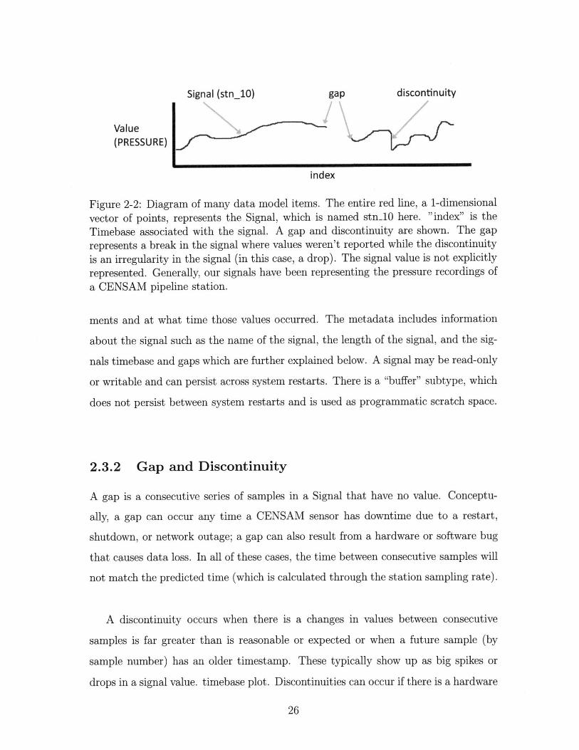
2-2 Diagram of many data model items. The entire red line, a 1-dimensional
vector of points, represents the Signal, which is named stn_10 here.
"index" is the Timebase associated with the signal. A gap and dis-
continuity are shown. The gap represents a break in the signal where
values weren't reported while the discontinuity is an irregularity in the
signal (in this case, a drop). The signal value is not explicitly rep-
resented. Generally, our signals have been representing the pressure
recordings of a CENSAM pipeline station. . . . . . . . . . . . . . . . 26
2-3 Diagram of Timebase graph demonstrating how Timebases allow for
powerful and easy conversion. Each node represents a Timebase and
each edge represents a TimebaseMetric. The green edges are Empirical
TimebaseMetrics, as the mapping is a list of points from data. The
purple edge is Derived, as a linear relationship exists between Seconds
and kiloH z. . . . . . . . . . . . . . . . . . . . . . . . . . . . . . . . . 27
2-4 Diagram of the entire Processing System. The API provides an ab-
straction for accessing the sysdata files, which the Importer created.
The Access Scheduler uses the API to expose functionality to Python.
The csignal module serves as the wrapper between the C++ API and
the Python world. End-users have the option of developing applica-
tions in Python or C++. Python users have the additional benefit
of being able to use the Access Scheduler to boost their application's
perform ance. . . . . . . . . . . . . . . . . . . . . . . . . . . . . . . . 30

3-1 Diagram of the behavior of the data importer. It takes a set of raw sig-
nal files as input and produces a group of files designed for our system.
Three files are created: the Intermediate Data file, the metadata file,
and the Timebase file. The Intermediate data file contains the actually
signal value data. The metadata file contains information associated
with the signal. The Timebase file contains an Empirical Timebase
providing a conversion between the signal's Timebase and Seconds. . 32
4-1 Diagram of how the Access Scheduler and Multiprocessor interfaces
with the rest of the Processing System. The ASM is comprised of the
Executor and Tasklete Python classes. Both classes are exposed to the
end user. To run the ASM, the user wraps their desired functionality
in Taskletes and feed those Taskletes to the Executor. The user uses
the Csignal API in combination with the Executor and Taskletes to
run the A SM . . . . . . . . . . . . . . . . . . . . . . . . . . . . . . . . 61
4-2 Diagram of the ASM dataflow for the FFT Adder Application. Rect-
angles represent Taskletes and ovals represent Signals. Here, Tasklete
1 reads in a segment of Signal A, FFTs that segment, and writes the
FFT results out to Buffer A. Tasklete 2 does the same with a portion
of Signal 2 and Buffer B. Tasklete 3 reads in these segments of Buffer A
and B, adds them, and writes the sum to the Output Signal. Tasklete
3 has dependencies on Tasklete 1 and 2 and will not run until they
have com pleted. . . . . . . . . . . . . . . . . . . . . . . . . . . . . . 62

4-3 Diagram of the primary ASM data structures and their interaction.
The Master process has Taskletes ordered to optimize performance
in the TaskleteRoster. A certain amount of these are added to the
Jobs Queue. The Worker Processes pop Taskletes off the Jobs Queue,
execute these Taskletes, and then place the completed Tasklete IDs
on the Newly Completed Taskletes Queue. The Master periodically
pops all Taskletes off this queue and adds the Tasklete IDs to the
completedTaskletes Dictionary. . . . . . . . . . . . . . . . . . . . . . 67
5-1 Diagram of the behavior of our system's I/O. There are several layers
of caching: disk/RAID caching, memory page caching, and individual
caches on the CPU cores. Direct Memory Access from either a major
page fault, fread, or readahead trigger data to be read from the disk
into the page cache. This only happens if the requested page is not
already cached. Fread will read directly out of the page cache, while
mmap triggers reclaims. Minor faults, or reclaims, cause pages to get
placed into the page directory, from which mmap directly reads. . . 78
6-1 Plot of Signal implementation runs of Scan Summarize with different
loads. X-axis represents data processed in Megabytes Y-axis is Total
Loop time in seconds. The theoretical maximum is computed using
our systems' maximum throughput. . . . . . . . . . . . . . . . . . . 98
6-2 Plot of ASM speedup for Windowed FFT application. X-axis repre-
sents number of workers. Y-axis is speedup using the base value of 1
w orker. . . . . . . . . . . . . . . . . . . . . . . . . . . . . . . . . . . 102
6-3 Plot of ASM speedup for Backwards scan with reordering. X-axis
represents number of workers. Y-axis is speedup using the base value of
1 worker. Naturally, we don't see an improvement with more workers,
as we are I/O bound. . . . . . . . . . . . . . . . . . . . . . . . . . . 106
6-4 Plot of ASM speedup for FFT Adder application. X-axis represents
number of workers. Y-axis is speedup using the base value of 1 worker. 110

12

List of Tables
5.1 Key system specifications, measurements, and parameters. . . . . . . 76
5.2 Summary results from profiling tests of different implementations of
Scan Summarize. There are 3 trials per version, all of which are fairly
close in value. Times listed in seconds. . . . . . . . . . . . . . . . . . 84
5.3 Summary page fault and reclaim results from tests of different im-
plementations of Scan Summarize. Multiple trials were run but results
were identical between trials. The data load is 3.67 GB, or more specif-
ically 3,947,364,352 bytes. This is exactly 963712 pages. . . . . . . . 85
5.4 Derived System Parameters. . . . . . . . . . . . . . . . . . . . . . . 93
6.1 Summary results from profiling tests of different implementations of
Scan Summarize. There are 3 trials per version, all of which are fairly
close in value. Times listed in seconds. For a more thorough breakdown
of these tests, see Table 5.2. . . . . . . . . . . . . . . . . . . . . . . . 97
6.2 Windowed FFT C++, Linear Python, and single worker ASM runs.
Total time includes initialization and startup (loading signal sysdata,
importing packages, etc.). Total Loop is the cost of reading signal data
and processing and has no applicable value for single worker ASM.
Times listed in seconds. . . . . . . . . . . . . . . . . . . . . . . . . . 99

6.3 ASM FFT with 1 worker results. Total time includes initialization and
startup (loading signal sysdata, importing packages, etc.). Preprocess-
ing is the time for the Preprocessing stage of the ASM (creating the
Taskletes, etc.), as described in Section 4.5.4. Execution is the time
actually running the ASM, though technically includes both the Pre-
execution (Section 4.5.5) and the Execution Stages (Section 4.5.6). For
reference, these totals are compared to serial implementations in Table
6.2. Times listed in seconds. . . . . . . . . . . . . . . . . . . . . . . 101
6.4 C++ scan forward, C++ scan backwards, and Python Scan Backwards
test results. The C++ Scan Forwards results were first displayed in
Table 5.2. Slowdown is relative to median C++ Scan Forwards case.
Times listed in seconds. . . . . . . . . . . . . . . . . . . . . . . . . . 103
6.5 ASM with one worker scan backwards without ordering. Times listed
in seconds. ....... ................................ 104
6.6 ASM with one worker scan backwards with ordering. Times listed in
seconds. ....... .................................. 104
6.7 Single worker ASM results for the FFT Adder application. . . . . . . 109

List of Listing
3.1 The algorithm for importing data into the system for processing. . . 34
3.2 The algorithm for detecting a gap or discontinuity in data . . . . . . 37
5.1 Profiling code using the Time Stamp Counter register. . . . . . . . . 80
5.2 The linux script we used to clear the memory caches. . . . . . . . . . 81
5.3 Scan Summarize application pseudocode . . . . . . . . . . . . . . . . 82

16

Chapter 1
Introduction
Many scientific research projects involve processing and analyzing large quantities of
data. However, as the size and complexity of the data sets increase, managing these
data sets becomes outside the scope of many analysis tools. When dealing with such
large amount of data, fundamental system constraints that usually may be ignored
become relevant. RAM is limited in size; many common and useful analysis appli-
cations (eg Matlab) have either an intrinsic or practical size limitation on imports;
seeking on a hard disk is time-intensive; and so forth. The Wavescope, an ongo-
ing project worked on by Dr. Girod and Prof. Madden at MIT CSAIL, provides a
platform for building distributed systems to capture and process high rate sensor data.
This MEng project involved designing, implementing, and testing a system that
provides a powerful yet relatively intuitive and simple interface for accessing, manip-
ulating, and analyzing large quantities of data. As such, our work has taken all of
the aforementioned constraints into consideration. In particular, we have carefully
designed, implemented, and evaluated a storage manager and processing system for
the CENSAM Pipeline project [7] ; the pipeline's distributed sensor network has been
collecting terabytes of data that our system allows scientists and engineers to analyze
and process.
The project is divided into three primary subcomponents.

The sensor network, rightfully focused on reliably recording accurate pressure data
from the pipeline , stores the data in a series of timestamped binary files that is cum-
bersome to index. Further, the data is often inconsistent, riddled with reflections of
changes to the recording system, errors and bugs with that system, and the same
noise that is to be expected in any such sophisticated sensor system. With this in
mind, our first task, was to devise a process for cleaning this data and convert it to
a format more conducive to analysis and processing.
The next component involved the creation of the actual processing system and its
API. As can be expected when dealing with such large amount of data, our primary
design challenge was performance. With this in mind, our work involved developing
our own internal data format, implementing and evaluating several different versions
that each have different low-level I/O procedures, and utilizing the full capacity of the
system's resources through multiprocessing and the creation of an intelligent access
scheduling system.
Finally, we rigorously experimented to measure the different implementations' per-
formances and determine which implementations are best and why this is the case.
In doing this, we painstakingly analyzed our system and developed a solid grasp on
its low-level I/O behavior and performance. The result is an accurate system model
for each of the different implementations of our processing system. Next, we analyzed
many variations, implementations, and pieces of our system to bettervn understand
its behavior and optimize overall performance.
Despite the specificity of our system around the CENSAM project, our results are
fairly generic and, we believe, widely applicable to many bulk-data systems.
1.1 Goals of the Project
Our overall project had specific criteria and high-level requirements that guided our
work.
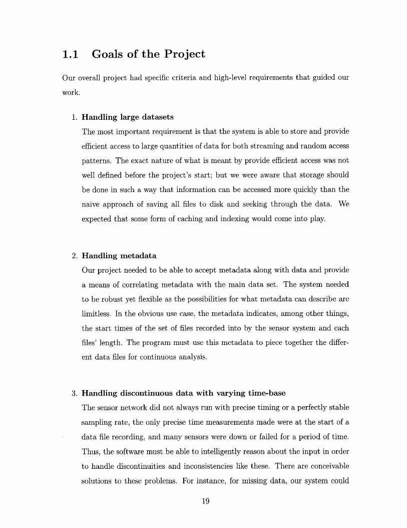
1. Handling large datasets
The most important requirement is that the system is able to store and provide
efficient access to large quantities of data for both streaming and random access
patterns. The exact nature of what is meant by provide efficient access was not
well defined before the project's start; but we were aware that storage should
be done in such a way that information can be accessed more quickly than the
naive approach of saving all files to disk and seeking through the data. We
expected that some form of caching and indexing would come into play.
2. Handling metadata
Our project needed to be able to accept metadata along with data and provide
a means of correlating metadata with the main data set. The system needed
to be robust yet flexible as the possibilities for what metadata can describe are
limitless. In the obvious use case, the metadata indicates, among other things,
the start times of the set of files recorded into by the sensor system and each
files' length. The program must use this metadata to piece together the differ-
ent data files for continuous analysis.
3. Handling discontinuous data with varying time-base
The sensor network did not always run with precise timing or a perfectly stable
sampling rate, the only precise time measurements made were at the start of a
data file recording, and many sensors were down or failed for a period of time.
Thus, the software must be able to intelligently reason about the input in order
to handle discontinuities and inconsistencies like these. There are conceivable
solutions to these problems. For instance, for missing data, our system could

draw a best-fit line between the two adjacent time-marked points, and use that
line to interpolate a given point's absolute time.
4. Present views to the user/application developer
End-user specified views must be supported. One could imagine the use case of
needing to decimate data and achieving this by presenting data in a decimated
view. These views must not only be presentable to users they should be ac-
cessible programmatically. This allows for more complicated analysis through
another application.
5. Provide programmatic interface
The project should provide interfaces for more complicated data analysis than
that provided in views. There are many options for satisfying this requirement:
a Matlab plugin, the WaveScope language WaveScript, or by simply allowing
users to write C-code (or code in some other programming language).
1.2 Related Work
A variety of work in the field of signal processing and signal storage management has
been done.
Developed at CSAIL by Prof. Madden and Dr. Girod (among others), WaveScope
provides a platform for building distributed sensing systems to capture and pro-
cess signals. The technology consists of several innovative functionalities. First,
WaveScope introduces a signal segment data type, which provide efficient operation
on data and an efficient means to pass signal data through a dataflow graph. Sec-
ond, it provides end-users with a novel programming language that minimizes data
conversion between applications/databases thereby reducing end-user programming

effort and boosting performance [3]. Lastly, executed queries can be distributed across
many nodes; this is quite useful as many of WaveScopes target applications are in-
herently distributed due to their sensor networks [4] [2].
Current work in Wavescope has been designed for streaming and memory pro-
cessing without addressing storage issues. Our work on a WaveScope-compatible
storage manager enables the WaveScope system to efficiently process input streams
from stored data, run queries over that data, and store the results.
The TimeSeries DataBlade database system was designed to handle large-quantities
of time-related data [8]. It can be paired with auxiliary technology to handle huge
volumes of streaming, real-time data. The database system itself, however, has a
SQL-like interface not suited for the type of analysis that motivates our project. To
implement signal processing queries of the type supported by WaveScope, one would
need to expose a programmatic DataBlade API.
Borealis is a distributed stream processing engine that provides functionality for
dynamic revision of query results, dynamic query modification, and flexible opti-
mizations [9]. Like WaveScope, Borealis is focused on streaming data and does not
currently have a processing specialized storage manager to support high performance
access to stored signals. Our work might be applicable to Borealis with modification,
to enable Borealis VMS to run efficient queries over stored data.

22

Chapter 2
High Level System Design
2.1 Overview
The storage manager and processing system is comprised of several distinct compo-
nents and conceptual abstractions. We begin this chapter by a discussion of the key
principles we kept in mind when designing our system. Next, we go on to discuss that
to manage the complexity of data we are processing, we have come up with a data
model that provides nomenclature and abstraction. After that, we discuss the design
of the process of copying the data files produced by the sensor reading system into
our internal system format, known as importing. Lastly, we give a high-level overview
of the actual processing system, which provides an API for accessing and analyzing
the data and also a system for parallelizing and optimizing analysis algorithms.
2.2 Key Design Considerations
The fact that scientists and engineers working on the CENSAM project are dependent
upon using this project serves as the biggest underlying driving force for our design.
Resulting from this, we have had five main design considerations.
1. Correctness
Since our project has real world end-users, who will be using it for further

CENSAM files Import Process Sysdata files Init process API
Signal
Timebase
Intermediate data Time
Rangemetadata
Timebase data Private Implementation:
TimebaseNode
TimebaseMetric
Metadata (JSON)
Figure 2-1: Overall design of the entire storage management system.
research beyond the lifetime of our work, it is important that the system works
as claimed and produces accurate results. Given this requirement, we have
operated with the understanding that correctness is not absolute and there
are trade-offs to be made. While we have paid careful attention to producing
accurate results, we have also worked hard to keep the project in scope. For
instance, some of our data cleaning operations during the import phase could
probably be improved further, but instead of exerting too much effort on this,
we chose to focus on other areas more in-line with the big picture of our project.
2. Performance
Perhaps the largest constraint for which we optimized, system performance and
speed played a crucial role in our design. As stated in our first high-level goal, we
strive to access large quantities of data faster and more conveniently than using
the ad-hoc format originally chosen for CENSAM data. We are not concerned
with system start-up, preprocessing, import, or shutdown performance, and are
concerned with steady state data processing operations.

3. Maintainability
As is typical of research code, the implementation work on this project has a
relatively short lifespan. In order to increase the likelihood that this system
has continued use throughout the longer term CENSAM project (and perhaps
beyond), it has been important to ensure the system and code is easily main-
tainable. As a corollary, it is important that others can easily understand the
system and its code-base so others can maintain it.
4. Extensibility
It is important that the system is easily extendible to match the potentially
changing requirements and nature of the CENSAM project. Further, while our
primary driving focus has been CENSAM, we have aimed to create a system
modular enough that it can be used in other projects and environments with
relatively little difficultly.
5. Usability
While our primary user-base is inherently technical, we have kept in mind the
importance of keeping our system fairly easy to use. Maintaining a clean and
straight-forward API and installation procedure along with the use of preexist-
ing tools like Python NumPy, will improve our system's adoption rate and the
ease with which others can maintain and extend it.
2.3 Data model
Our data model is comprised of several concepts: a signal, timebase, gap, discontinu-
ity, time, and range.
2.3.1 Signal
A signal is a vector of 1-dimensional points and associated metadata, representing a
continuous sampling process. In essence, a signal is comprised of a series of measure-
Signal (stn_10) gap
Value(PRESSURE)
index
Figure 2-2: Diagram of many data model items. The entire red line, a 1-dimensionalvector of points, represents the Signal, which is named stn-10 here. "index" is theTimebase associated with the signal. A gap and discontinuity are shown. The gaprepresents a break in the signal where values weren't reported while the discontinuityis an irregularity in the signal (in this case, a drop). The signal value is not explicitlyrepresented. Generally, our signals have been representing the pressure recordings ofa CENSAM pipeline station.
ments and at what time those values occurred. The metadata includes information
about the signal such as the name of the signal, the length of the signal, and the sig-
nals timebase and gaps which are further explained below. A signal may be read-only
or writable and can persist across system restarts. There is a "buffer" subtype, which
does not persist between system restarts and is used as programmatic scratch space.
2.3.2 Gap and Discontinuity
A gap is a consecutive series of samples in a Signal that have no value. Conceptu-
ally, a gap can occur any time a CENSAM sensor has downtime due to a restart,
shutdown, or network outage; a gap can also result from a hardware or software bug
that causes data loss. In all of these cases, the time between consecutive samples will
not match the predicted time (which is calculated through the station sampling rate).
A discontinuity occurs when there is a changes in values between consecutive
samples is far greater than is reasonable or expected or when a future sample (by
sample number) has an older timestamp. These typically show up as big spikes or
drops in a signal value. timebase plot. Discontinuities can occur if there is a hardware
discontinuity

or software error that causes dropped samples or erratic values, or when timestamps
are recorded before GPS lock has been established.
2.3.3 Timebase
Stn; 10 & Seconds Metric
Seconds KiIoHz%Metric
St a111 Met icStn 10 & Stn 11 Metric
Figure 2-3: Diagram of Timebase graph demonstrating how Timebases allow for pow-erful and easy conversion. Each node represents a Timebase and each edge represents
a TimebaseMetric. The green edges are Empirical TimebaseMetrics, as the mappingis a list of points from data. The purple edge is Derived, as a linear relationship existsbetween Seconds and kiloHz.
The timebase abstraction represents the time dimension of a signal: a handle for
the unit of time exhibited on a signal plot's x-axis. Thus, a timebase conceptually
represents a unit of time. Seconds, CPU clock cycles, and the sample count of station
10 are representations of time and are therefore valid Timebases. Every signal has a
single timebase associated with it in its metadata. [2]
We decided to abstract away the time-value of a signal because a common use-case
is to make comparisons between signals that have different timebases, but that have
some empirical conversion relationship. For instance, a CENSAM sensor station by
default has a timebase unique for that station; that is, the sample clock at a station
is locally linear, thus the sample count is the most precise way to annotate the time
at which a sample was captured. Each station, therefore, has its own mapping of

indices to seconds based in GPS.
Thus, in order to compare two separate CENSAM sensor station readings (which
CENSAM researchers would want to do for such things as detecting a leak), we can
convert a station's timebase to that of another station's by constructing a relational
graph of all of the timebases. In this example, a station can be compared to another
by first converting to Seconds and then to that second timebase. Further, since there
is a relationship between Seconds and other values, we can readily remap a Signal
onto other time axes.
These relationships can be defined using a graph model. Each node on the graph is
a Timebase and each edge is a TimebaseMetric. Thus, a TimebaseMetric represents a
relationship between two Timebases. There are two kinds of relationships: empirical
and derived. An empirical metric is a mapping defined by an explicit correspondence
of values between two Timebases - that is, list of pairs of corresponding points, e.g.
station 10 sample number and second. A derived metric is a linear equation relating
two Timebases. Derived metrics are used to perform time unit conversions.
2.3.4 Time and Range
As with any system dealing with signal processing, it is natural that our system have
a way of representing a single point in time. We created a separate Time object to
encapsulate this concept. To represent a point in time we use a pair of a double and
a Timebase. A Time can be thought of as a value with its unit, as in 3 seconds,
or the 3rd station 10 sample. By explicitly including the time unit with the value,
we can easily convert a Time point in one Timebase to that in another and avoid
confusing in which Timebase a value is measured. A range is simply a pair of Times
- representing a beginning and an end.

2.4 Importing Data
The system imports data into a special system format before that data can be used.
Since this is a one-time process, we don't focus on the performance of the import
process. Given the large variation in existing data representations, we did not at-
tempt to design a universal import API. Rather, we constructed a CENSAM-specific
importer. However, much of the techniques and discussion regarding our CENSAM
importer can be easily applied to other importers.
For a single signal import, the system outputs 3 system data files: the intermedi-
ate data file, the metadata file, and the timebase file. With our CENSAM example,
we have create a signal for every station, so each station produces 3 files. The import
process also detects gaps and discontinuities to place the data into a consistent and
coherent timebase.
Once any particular data set is converted to the system data format, the pro-
cessing system will work fine with it. That is, the application-specific details of the
import system is encapsulated away from the rest of the system and once a data-
specific importer is written the rest of the system will perform as well as it does with
the CENSAM data.
2.5 Processing System
The Processing System is the primary design and implementation component of the
Storage Manager System. As such, significant design thought and effort went into its
creation.
The Processing System is comprised of many components. The previously dis-
cussed Sysdata files are the datastore for signals and all persistent information. Writ-

ten in C++, the API exposes a simple yet powerful interface for creating, accessing,
and modifying, Sysdata files. Since the primary abstract data type in the API is
the Signal, we generally refer to the API as the Signal API. The csignal module is a
wrapper over the Signal API that exposes its functionality to Python. The primary
end-client of the csignal wrapper is the Access Scheduler, a Python module written to
optimize the runtime of users' queries, although csignal is by no means encapsulated
by the Access Scheduler.
Sysdata files API Access Scheduler User Apps
Executor
Timebase Csignal Taskete User PythonIntermediate data Application
Time
metadataUser C++
Timebase data -0 -- *-*--- - - - pctoApplication
Figure 2-4: Diagram of the entire Processing System. The API provides an abstrac-tion for accessing the sysdata files, which the Importer created. The Access Scheduleruses the API to expose functionality to Python. The csignal module serves as thewrapper between the C++ API and the Python world. End-users have the option ofdeveloping applications in Python or C++. Python users have the additional benefitof being able to use the Access Scheduler to boost their application's performance.
In the end, we are left with a powerful, high-performance system that can quickly
perform complicated operations on the huge amount of data that is stored in the
system. The system in flexible in that users can choose to develop in either Python
or C++. Further, we were able to design our Python modules in such a way as to
ensure there is not really a significant performance hit. And if a user does develop in
Python, they have the benefit of having the Processing System optimize their perfor-
mance.

Chapter 3
Design and Implementation of the
Importer
While the Importer is not the main focus of our work, it is an essential component
to our system. As the majority of our work centered around designing, implementing
and optimizing the processing system, a good amount of thought went into designing
an optimizing format in which the processing system's data is stored. Naturally, the
design of this format impacts the Importer's design considerations and constraints
and import algorithm. Further, the data must be massaged and cleaned up the data
so that it is in a state ready for practical analysis. One notable difference in require-
ments for the Importer is that since the import process only occurs once, we were not
concerned with optimizing its performance.
3.1 CENSAM Data Files
We worked with the CENSAM pressure sensor data set. Although the importer we
made is custom to this particular dataset, the principles apply more generally.
There are approximately 15 stations in the dataset. While the present and valid
data for each station is not consistent among stations, each station has about a years'

Concatenation of all CENSAMntermediate data station files into a single raw data
file spaced appropriately for gaps
Station 10JSOIN file with associated info
Ftie 0 metadata (name, station id, number ofsamples, last sample index, list ofgaps and discontinuities, etc.)
Timebase data Contains Timebase mappings (ie -series of index points to seconds).
Figure 3-1: Diagram of the behavior of the data importer. It takes a set of raw signalfiles as input and produces a group of files designed for our system. Three files arecreated: the Intermediate Data file, the metadata file, and the Timebase file. TheIntermediate data file contains the actually signal value data. The metadata file con-tains information associated with the signal. The Timebase file contains an EmpiricalTimebase providing a conversion between the signal's Timebase and Seconds.
worth of days in pressure data. Many of the stations have other sensor data (temper-
ature, battery, etc.), We worked primarily with station 10 pressure data, which has
372 days present in total.
The data is organized into a directory hierarchy of station, year, day, and lastly
sensor-type. That sensor-type directory contains all the data files for that given day
and sensor-type. This scheme was a design decision of the sensor system and from
our perspective was a preexisting choice.
The pressure files are 120,000-byte raw-data files where each 2-byte value is an
individual sample stored consecutively. Thus, each file contains 60,000 samples, rep-
resenting a 30-second sampling segment. The system has a nominal sampling rate of
2 kHz. These values are consistent since (60, 000)/(2kHz) = 30 secs. On a day when
the sensor does not malfunction and produces all the data files, there are 2,880 files
per day (since 2, 880 * 30 = 24 * 60 * 60).

We import these data files into the Intermediate Data Format, one sequential
sparse binary, which is discussed in detail in Section 3.3. In this format, station 10's
data amounts to about 60 Gigs. Note that because our imported system data file is
sparse, it should be more compact than CENSAM Data Files. Still, their size should
not be more than a factor of 2 greater (in fact, assuming perfect recording, the CEN-
SAM files would be 2, 880 * 372 * 60, 000 *2 bytes 120 GB, which is about twice the
size of our imported data.
Each file is named with the station name and a timestamp of the first sample
with second accuracy. From these stamps, we can verify that each file contains 30
seconds of data. More importantly, this characteristic will become crucial for gap and
discontinuity detection.
3.2 Import Algorithm
The import algorithm scans all of a signal's disparate files sequentially and produces
the appropriate system data files in a consistent and accessible format. While iterat-
ing through the original signal files, the algorithm checks for gaps and discontinuities.

function importStation(stnname) {
Create EmpiricalTimebaseMetric between stnname and Seconds
Create a Metadata file for stn-name
Create an IntermediateData file for stnname
Sort all files for stn-name
Iterate through sorted file list:
Compute Exponential Windowed Moving Average with prev file
If there was a gap or discontinuity:
Mark this in Metadata file and
Increment/decrease index // ensures the file is sparse
Write file data to iData file
Write empirical mapping to TimebaseMetric file
Write number samples, end index, etc. to Metadata file
}
Listing 3.1: The algorithm for importing data into the system for processing.
3.2.1 Gap Detection and Compensation
Although our import procedure will only detect gaps and discontinuities between file
boundaries and not on samples inside files, this is a limitation of the original data
format. This allows us to avoid the painful process of iterating through every entry
in every file and performing more complicated data massaging and detection algo-
rithms. Further, we have been focusing on the huge-data cases; small glitches within
30-second files will be negligible when dealing with days and perhaps months worth
of data.
Key to our gap detection and compensation algorithm is prediction of the sampling
frequency. While, we know the CENSAM sensors' sampling frequency is set to a
nominal value of 2 kHz and is locally linear, the sensor system's clock frequency will
drift over time such that the sampling does not occur precisely at 2 kHz. In addition,
each timestamp will have some measurement error associated with it.

Despite the variance in actual sampling frequency, the file timestamps we are
given are from GPS and therefore are accurate despite some degree of imprecision
from sampling error. Thus, using the timestamps and number of samples in a file,
we can predict the average sampling frequency over the file. Given that we expect
slippage to be minimal, we can use this computed value as a better approximation
of local frequency. In fact, we can combine this value with neighboring files' own
computed frequencies to obtain an even better approximation.
Having a good approximation of the local frequency is necessary when dealing
with gaps for two reasons. First, given that we have reliable values for only the start
of each file and the number of samples in each file, we can use the approximate fre-
quency to predict the time of the last sample in a file. Given that we expect each file
to be adjacent, if there is a sufficient difference between the end sample timestamp
of one file and the begin sample timestamp of the next file, we detect a gap. Second,
having a good local frequency approximation enables the algorithm, after detecting a
gap, to extrapolate how many samples large that gap is and thereby compensate for
the gap.
Implementation
As discussed previously, because gap detection is coupled with import, the gap detec-
tion algorithm is embedded within the file import code. Our algorithm begins with
initialization of constants. In particular, the currentFrequency initializes its estimate
with what we were told was the actual polling frequency.
In the standard import procedure, we iterate over all the files. We compare the
difference between the timestamp of the beginning of the current file with the pro-
jected last timestamp of the previous file. This difference conceptually corresponds
to the time between files: if it is large, we have a gap and if it is negative, we have

a discontinuity. We allow for timestamp impression with the GAPSLIP constant
(which is set to 0.075 seconds). A discontinuity has a negative difference.
Once an irregularity detected, we estimate its size in samples by multiplying the
previously found time distance between files with the currently estimated polling fre-
quency. To compensate for the irregularity, we increment the running index (which
is used in normal import code to keep track of the current index of whatever is being
imported). We then record the gap or discontinuity in metadata.
At this point, we run the normal import code. This happens regardless of whether
or not an irregularity was detected. If we have compensated for a gap or discontinuity,
the effects from that impact normal import code through the change in size of the
running index.
As a final step, the algorithm must update its state. First, it estimates the end
timestamp of the end of the file by dividing the number of samples by the current
frequency and adding that to the beginning timestamp (recall that this value is used
when detecting irregularities at the start of the loop).
In what is perhaps seemingly the most complicated step, the algorithm uses pre-
viously computed values to update the current approximate frequency. First, we
compute the average frequency for the given file by dividing the files' sample count
(in addition to any samples it may have gained or lost from gaps and discontinu-
ities) by the difference between the previous files' start timestamp and this files' start
timestamp. This is the average frequency between files including irregularities. Then,
we combine this with the current running average frequency through the use of an
Exponentially Weighted Moving Average. The result is a more precise local frequency.

1 currentFreq= 2000.033
2 prev-file-endtimestamp = 0
3 lastfiletimestamp = 0
4 for file in sortedListOfImportFiles:
5 // detect gap and discontinuities
6 double gapSpace = file.starttimestamp -
7 prevfile.end-timestamp
8 bool wasGap = gapSpace > GAPSLIP
9 bool wasDiscontinuity = gap Space < 0;
10 if (wasGap || wasDiscontinuity) {
11 double indicesInGap = gapSpace*currentFreq;
12 running-import-index += indicesInGap
13 // save gap in metadata
14 recordgap-ordiscontinuity(index, indicesInGap, file)
15 }
16 // run the import file prcedoure
17 normalImportFileProcedure(running-import-index, file)
18 // approximate timestamp of last file sample
19 double fileSecs = file.num-samples/currentFreq
20 prev.file-end-timestamp = file.starttimestamp + fileSecs
21
22 // update approximate frequency based on what we now know
23 double secsBtwnFileTs = file.starttimestamp -
24 last-file-timestamp
25 double localFreq = (file.samples + gapSpace)/secsBtwnFileTs
26 // update current frequency using EWMA formula
27 currentFreq= alpha*curentFrequency + (1-alpha)*localFreq
28
29 last-file-timestamp = file.starttimestamp
Listing 3.2: The algorithm for detecting a gap or discontinuity in data
An Exponentially Weighted Moving Average is a moving average where the weight
of each future data point decreases exponentially. In doing this, we ensure future
changes impact the change in estimated frequency slowly. We define the EWMA
using the formula Ri = R * a + A * (1 - a).
We used the following parameter values:
a = 0.999999,
Ro = 2000.033
3.3 Intermediate Data format
Our Intermediate Data Files contain all signal value data. Each signal has one single
IData file. The Intermediate Data file is thus a concatenation of all signal RAW files
in sorted order with appropriate spacing for gaps. That is, every samplesize bytes
contains a distinct sample or the n sample begins at the n * samplesizeth byte and is
of length samplesize. We chose this format for several reasons.
First, the approach allows for a very simple lookup algorithm, which is
sampleValue(n) = n * samplesize
We use O/S facilities where possible and only invent new ones if needed. Hav-
ing a simple algorithm helps with implementation, testing, and thereby increases the
chance of correctness. Further, the algorithm requires very little processing. It also
allows for easy debugging.
Second, having contents in a single file optimizes for the use-case of scanning a file.
We believe this is a common use case for large signal processing because in order to

understand the data, it often makes sense to summarize large chunks of consecutive
data (ie - by taking averages). Further, by the spatial principle of locality, values
logically sequential or related are highly likely to be accessed together. Storing data
sequentially guarantees that a block on the hard disk will have an ordered list of
sequential samples. Since we are using a single file, it is highly likely blocks are also
stored sequentially on disk. This in turn, takes advantage of the system's multitude
readahead operations (some of which occur at the hardware level, some in the oper-
ating system, and some by our specific application).
Third, creating the file is simple and painless with our sequential import algorithm,
defined in Figure 3.1. This reduces the possibility of errors and thereby increases cor-
rectness.
A benefit of having sequentially-mapped files is that by only writing segments
that are used, the file will maintain a consistent time index without consuming the
extra space.
3.4 Metadata
Metadata files contain all remaining signal information that is not stored in the In-
termediate Data File. This includes information that can be derived from the IData
File but is expensive to compute. Fields of the Metadata file include the number
of samples in a signal, the end sample index (which is different than the number of
samples since samples omitted due to gaps have indices), the signal's nominal rate,
and a log of "events" that occurred in the signal.
Currently, the log is used to annotate gaps and discontinuities. A gap contains
a starting index, a length, and some debugging information (original file and times-
tamp). A discontinuity contains only a index and original file for debugging. We use

this log to track which parts of the IData are valid signal data and which are gaps.
The log is implemented as a sorted list of log events. A log event contains an
identifying tag, and any number of custom values (which are dependent upon the log
type). This allows for extreme flexibility and extensibility; we can easily add infor-
mation about different parts of the signal to the log.
The Metadata files are not intended to hold a huge amount of data. For example,
station 10 has 60 IData file, but the Metadata file is only 512KB. Fortunately, this
easily fits in memory and we did not have to focus on optimizing its design for per-
formance. We chose to implement it in JSON due to the availability of APIs and its
readability.
3.5 Timebases
A Timebase file represents an Empirical Timebase Metric between the current signal's
indices and seconds. As such, it contains some information about the metric (such as
the peer Timebase's nodes) and the type of the Timebase Metric (derived timebases
also have Timebase files, but these are never created on import).
To define the relation from one timebase to another, the file contains a list of
corresponding points in two timebases. We record one pair of corresponding points
for each timestamp defined in the input data (that is, one pair for each file). Since
the majority of samples in a signal does not have a direct mapping, it is the responsi-
bility of the processing system to interpolate between adjacent corresponding points
to estimate a timestamp value for a given sample, and vice versa.
Timebase Metric files are much larger than Metadata files, but are still substan-
tially smaller than IData files. Station 10, for instance, has a 32 MB Metadata file.

While this is fairly large, it is still small enough to easily fit into RAM, and we do
not consider the scaling impact of timebases on processing system performance. For
similar reasons to those discussed in the Metadata section, we also save Timebase
files in JSON.

42

Chapter 4
Design and Implementation of the
Processing System
The design and implementation of the Processing System is the main implementation
effort of this work. The system enables efficient processing of very large quantities of
data through optimized disk I/O strategies, a usable and flexible API, and a sophis-
ticated scheduling and multiprocessing module.
4.1 Initialization Process
Upon system startup, the Processing System goes through an initialization stage
where it loads the appropriate Timebase and TimebaseMetrics into memory from
Sysdata files. We are not concerned with the performance of this aspect of the
system, as we are more focused on the runtime performance of steady state Signal
operations. Note that neither Signals nor their metadata are preloaded at this stage;
that happens upon specific Signal loading.

4.2 Signal API
The Signal API is intended to provide a powerful yet simple interface for accessing,
modifying, and creating Sysdata. It is designed for high-performance behavior with
large quantities of data. As such, it is written with a combination of low-level C and
C++.
The interface is entirely exposed in C++. Despite the complexity and many mov-
ing parts of what the Signal API is abstracting away, we end up exposing only a
handful of classes that provide sufficient functionality: Signal, Timebase, Time, and
Range.
4.2.1 Signal class
The Signal class is the primary abstraction in the Processing System API. It repre-
sents a signal, as defined and discussed in Section 2.3.1.
During the design process we experimented with several different implementa-
tions of Signal. The differences all centered around low-level disk I/O techniques
and, besides performance, all implementations behave the same. Our strategy was
to begin with the simplest implementation and increase complexity of our solution
incrementally as warranted by performance gains. See Section 4.4 for a discussion of
the different Signal implementations.
Initializing
One can either open a preexisting signal or create a new one. When opening, a signal
can be read only or writable; read-only is useful for important signals that should be
immutable, ie input data sets.
During the creation of a signal, internal Metadata and Timebase data structures

are created. These are written to disk upon a call to Signal's save method (discussed
below). Users have the option of truncating a new signal, in which case, if an old
signal exists with an identical name, it will be replaced.
When opening, the Signal loads all metadata into memory, including gaps and
discontinuities. As discussed in Section 3.4, Metadata files are inconsequential in
size, so we can neglect the cost of loading. Also, as a reminder, we do not attempt to
optimize initialization costs since they are one-time costs and are negligible in com-
parison to the steady state costs when the system is run over large data sets.
Gaps and discontinuities are then stored in an internal vector data structure. A
Gap is represented as a Range, which as explained in 2.3.4 is simply a pair of times.
It may seem as though storing all gaps internally could be a wasteful use of system
memory, but we found this not to be true. Given that we only detect gaps between
files (see: 3.2.1), in the worst case of 2 years' worth of data with a gap per file, with
an unoptimized 300 byte Range implementation, the gaps data structure is still less
than half a gigabyte. Storing gap data in memory lowers the cost of iterations over
contiguous portions of a signal, which is a common use case.
In general, we've determined that binary searching through gaps lists to be an
adequate search strategy. Some speedup could be achieved through implementation
of a more complicated gaps data structure, but we leave this to future work.
Buffered Types
Signals can also be "buffered" in the case that they do not need to be saved. Buffered
Signals has an Intermediate Data file, but whenever the Signal is garbage collected,
the file is deleted. Metadata and Timebase/TimebaseMetrics for the Signal cannot
be written out.

Buffered Signals were created due to the need to have temporary space during
computation. In particular, certain implementations of Signal use shared memory
(discussed later) and Buffered Signals are used in the Scheduler/Optimizer for inter-
process communication. We provide a separate factory creation method for making
Buffered Signals.
Accessing and Modifying data
The access mechanism for data is a function called ptr(). It accepts a Range and
returns a pointer to a contiguous region of RAM containing the corresponding data.
Note that ptr() does not guarantee that the data has been paged in from disk (this
is implementation dependent). It is the responsibility of the client to call release()
in order to appropriately clean up the memory space when the data is no longer used.
Note that since ptr() takes a range as an argument, it is possible to ask for a set
of data using Range, defined in a timebase other than the Signal's native timebase.
For instance, one could conceive of needing to investigate a leak that seemed to occur
at 12:30AM on a given day. Instead of worrying about the station's sample to Sec-
ond conversion, one can simply pass pointer a range in the Seconds Timebase with
timestamps of midnight and 1AM for the given day.
Ptr 0 requests a read only region of memory; there is a another function writePtr 0
for requesting a writable region. By making each request explicit about which signal
sections are writable and which aren't, the implementation is better able to optimize
access. For example, if there is additional cost for writable segments, writePtr 0
can implement its own algorithm for the cost unique to writing. There is also an
append() operation that extends the size of a signal and adds samples onto the end.

Gap Functionality
The primary use-case for gap data has been to check if a given region contains or over-
laps a gap. Thus, we provide the contiguous() procedure which accepts a Range
and returns true if no gaps exist in or overlap the end points of the region. The
implementation involves binary search algorithm variant of the gap list to find a gap
in violation.
For writable signals, we provide appendGap 0. It is currently not possible to insert
a gap into a signal.
Saving
Signal's save ( function is applicable only to writable signals (and, in particular, not
Buffered signals). It writes a Signal's metadata and Timebase information to disk.
The operation is intended to be used once - after a signal is created or one is modified
with the intention of being reused later.
Save ( does not necessarily write out Intermediate Data - that is implementation
dependent and typically happens when the data structure is written to.
The Process Manager is not fault-tolerant. That is, if an application is interrupted
or crashes, the signal will be irrecoverable; the Metadata and Timebase information
will not be saved. Note that it is possible that the Intermediate Data may be intact
or partially written, but this information is contextually useless. Fault tolerance can
be implemented by logging changes to the data and using a write-ahead discipline,
but this was outside the scope of this project.

Auxiliary functions
The API also include several auxiliary functions. Many of these functions manipu-
late the Signal Metadata. For a discussion of data contained in a Metadata File, see
section 3.4.
sampleCount 0 returns the total number of valid samples (excluding gaps).
endIndex() and startIndex() return the corresponding indices in the Signal's
timebase (these return 64-bit integers, not Time objects).
indexOf () accepts a Time or Range in any Timebase and returns either a Time
or Range in the signal's Timebase (with its value converted appropriately). This
conversion function is a simple wrapper around functionality encapsulated in Time
and Range, which is discussed in Section 4.2.3.
inbounds () accepts a range and returns true if that range does not extend before
the start of signal or after its end. Like with indexOf 0, Timebase conversion is
taking care of through Range.
4.2.2 Timebase
The Timebase system is implemented behind abstract data types. Both TimebaseN-
ode and TimebaseMetric are essential datatypes to the Timebase model. [2]
While Timebase represents a unit of time exhibited on the x-axis, it has a very
simple implementation. In the API, a Timebase is simply a handle, a mapping to a
TimebaseNode.
A TimebaseNode contains a name and a vector of TimebaseMetrics that relate

between TimebaseNodes.
A TimebaseMetric is an edge in the Timebase graph that relates two TimebaseN-
odes - an edge in the Timebase graph. It therefore contains two "peer" TimebaseN-
odes. A TimebaseMetric can either be Derived or Empirical. A Derived Timebase-
Metric contains the linear equation that relates the two peer TimebaseNodes defined
by a slope and x- and y- offset. An EmpiricalTimebaseMetric contains a vector of
value-pairs, representing a mapping of points from one TimebaseNode to another.
The true heart of the Timebase system lies in the TimebaseMetric Convert 0
function, which transforms a numeric value from one peer Timebase to another. For
DerivedTimebases, this amounts to evaluating the linear transformation function at
the given point.
The implementation of an EmpiricalTimebaseMetric is more complex. Recall that
an empirical metric is defined by a set of discrete corresponding points that relate
one Timebase to another. That is, it may know that sample 100 happened at second
30 but sample 200 occurred at second 63. In this case, when Convert 0 is called
from indices to seconds on index 100 or 200, the answer is computed trivially. In the
other cases, we must interpolate between two points, or, for edge cases extrapolate.
The algorithm uses a binary search variant on the vector of value-pairs, to find either
the matching index or the neighboring points that include the value for which the
algorithm is searching.
Note that the low level Convert 0 method of TimebaseMetric will only convert
between adjacent TimebaseNodes in the graph - that is, they must share a Time-
baseMetric. To understand how the system converts between any arbitrary nodes in
a connected graph, see 4.2.3.

4.2.3 Time and Range class
Time and Range have very straight forward implementations.
Time
As discussed in 2.3.4, a Time is simply a Timebase paired with a double value. Be-
sides some overloaded arithmetic and comparison operators, a Time has accessors to
its Timebase and value, and a Convert InPlace 0 function.
ConvertInPlace()
Convert InPlace () is where the real power of the Timebase and Time system exists.
While Timebase's Convert () function converts Time values between adjacent nodes,
Convert InPlace 0 will convert a given Time value to any arbitrary Timebase pro-
vided a path exists on the connected graph of TimebaseNodes and TimebaseMetrics.
It does this by performing a breadth-first-search through the nodes, a strategy that
guarantees returning the shortest path. Once the shortest path is found, Timebase's
Convert () function is iteratively called along the path, propagating the value from
the original Timebase to the final Timebase.
Range
A range is literally a pair of Times subject to the condition that both Times have
the same Timebase. It has accessors for its start and end Time, a length() function,
an overlaps() function, and its own ConvertInPlace(). length( simply returns
the numerical difference between the two Times. overlaps 0 accepts another Range
and returns true if that range includes the instance Range entirely. Its implementa-
tion has no surprises; it does this by Converting Times and comparing their values.
Convert InPlace 0 simply calls Convert 0 on both the start and end times with the

same values.
4.3 csignal Module
The csignal Module provides a Python wrapper around the Signal API. Using Python
speeded development, although it had the potential to reduce performance. Based on
this concern, we paid particular attention to validating runtime performance against
C++ throughout the design and development of the csignal Module.
4.3.1 Decision to Use Python
We decided to extend our system in Python for several reasons.
1. Ease of end user development. Python is known for fast development and
a quick learning curve. We believe that Python is an easier to use development
environment that would allow for faster creation of applications and would al-
low users to develop queries with fewer bugs. This would not only improve
the adoption rate and ease of use for the end user, but also enable more rapid
development and ultimately create a more sophisticated system.
2. Ease of runtime system development. Python provides great interfaces for
developing parallel and distributed programs, which are otherwise notoriously
difficult to implement. A multitude of other multiprocessing libraries are also
available for python such as delegate, forkmap, ppmap, pp, etc. [13]
3. Libraries and extensions. Python has an extensive scientific computing li-
brary that makes it easier for the end user to write application code. In partic-

ular, we believe the Python NumPy library is particularly useful.
4. Extensibility. We foresaw the possibility of one day extending the Storage
Manager and Access Scheduler to be a distributed system. In this case, Python
has a variety of libraries including batchlib, Celery, disco, exec-proxy, pp, etc.
Using Python reduced our development time and we found ways to work around
performance problems.
4.3.2 C Python API
Python provides a well documented C API that allows developers to write Python
wrappers around their C and C++ code. Using this API, we developed a Python
Signal class that wrapped our C++ class and exposed a multitude of other C/C++
functionality, while achieving performance comparable to the C version. [10]
4.3.3 Numpy Arrays
NumPy is Python's package for scientific computing. Our use of the NumPy li-
brary was key to achieving high performance with Python. On top of sophisticated
functions, tools for integrating with C/C++, and mathematical operations, NumPy
provides a high-performance N-dimensional array. We used this array to interface
with the Signal API.
As discussed in Section 4.2.1, the Signal API's primary method for accessing data
involves returning a C array. Python data types such as lists and tuples are not
optimized for fast access and are therefore not a viable option for our system. Even
if they were, having to convert between the native Signal API data structure (ie a

native C array) and Python types is costly. Beyond that, the structures would be
wasteful as Python does not have good support for scalar types.
Numpy Arrays, under the covers, are essentially a wrapper object around a native
C array. They are contiguously laid out in memory and support all the standard C
scalar types. Naturally, they offer constant time access and write.
We use Numpy Arrays as our main data type for the Python part of the processing
system. The Csignal module converts the C arrays returned from the main Signal
API into NumPy arrays; conversely, it accepts NumPy arrays and converts them to
C arrays. Since NumPy arrays are essentially C arrays, this conversion comes at no
cost and enables our system to operate at our high bar for performance in the Python
environment. [10]
4.3.4 csignal API
The csignal API provides a Python module named esignal which defines a class and
has a separate collection of utility functions. We discussed this set of auxiliary func-
tions in Section 4.3.5. The defined class is called Signal and provides essentially a
wrapper for the C Signal API, using NumPy arrays where appropriate.
4.3.5 Auxiliary Functionality
In order for the Signal API to be fully functional in Python, the csignal API exposes
some additional functionality beyond what is provided by the C Signal API. Some of
this functionality exposes low-level C procedures required in Python for optimization,
others wrap C functions that are simply better performing than their Python imple-
mentations, and others provide special functionality required for the multiprocessing
module.

fft()
Many of our tests involve computing Fast Fourier Transforms. The FFT procedure
provided in by NumPy was empirically slower than the C fftw package. The sim-
ple solution was to expose fftw to Python through a simple csignal. f f t () function,
which accepts a 1-dimensional NumPy array of real-values and returns a 2-dimensional
NumPy array containing the resulting FFT in the real and imaginary dimensions. [14]
fftFreeArray()
Due to implementation details of csignal. f f t (), manual memory management is re-
quired. f f tFreeArray () accepts a NumPy array of the type returned by csignal. f ft 0
and performs the necessary clean up to prevent memory leaks.
Readaheado
As discussed in Section 4.4, the low-level readahead() system call is used in the
Signal API implementation. We expose readahead() so the Access Scheduler and
Multiprocessor, discussed in Section 4.5 can optimize further. Being able to call
readahead() itself, the Scheduler can freely reorder file rewrites.
pinCPU(
We have discovered that our Multiprocessor runs faster when each individual process
is pinned to a core and is not reshuffled by the Operating System. As such, we expose
the low-level sched-setaf f inity () so the multiprocessor can lock a worker process
to a particular core.

getSignal()
The multiprocessor requires that different processes have access to the same set of
Signals and that the multiprocessing system has a simple way of identifying a Sig-
nal. getSignal 0 accepts a signal handle and returns a Signal. Under the hood, the
csignal module contains a vector of Signals where the index is used as Signal handle
(thus, all getSignal () does is merely accesses a vector).
4.4 Disk I/O and Signal Implementations
A key Signal API design decision was our decision of how to read and write data to
disk. The two options we had were using the C library function f read() with explicit
buffer allocation or utilizing memory-mapped I/O with the mmap() function. In the
former case, we would simply read chunks of sysdata files in batched amounts. The
latter involves directly mapping the sysdata files into address space and triggering a
disk access only when that part of the data is accessed. Because mmap() triggeres
the data to be loaded by the kernel page fault mechanism, it effectively does I/O in
parallel with program execution
To evaluate these alternatives, we decided to implement multiple versions and
run experiments to determine which method performs best. We found that mmap
ultimately won out due to both superior performance and simplicity.
4.4.1 Key Design Decisions
There were a number of design decisions we took into account when picking an im-
plementation method.

Sharing
Whether or not our data could easily be shared between processes was important.
Mmap maps files into shared memory, which allows the data to be accessed concur-
rently from multiple processes.
On demand read/write
In principle on demand read reads only as needed with no additional application com-
plexity. Write on demand writes out only pages that are modified without explicitly
tracking pages that are modified.
OS support
We can benefit from many of the optimizations implemented with the Linux Ker-
nel. For example paging, on-demand-writing, caching, etc. are already provided with
mmap. Using fread, we would need to implement a similar facility ourselves.
Complexity and Ease of Implementation
Each method has respective parts that are difficult to implement. It is difficult to
efficiently write back to disk using an fread technique; once data is read in and part
of it is modified, which data needs to be written back to disk must be tracked. On
the other hand, appending to a buffer established with mmap is cumbersome and
presents performance problems due to remapping overhead. Mmap o works by taking
a file and a start and end byte; thus, appending in such a situation requires unmap-
ping, artificially increasing the size of the file, and remapping.

Performance
Performance is our central design concern. Fread does a straight disk read and in that
sense is very fast and has minimal overhead. Mmap reads data on-demand through
page faulting and page reclaiming, which require traps into the kernel. Used naively,
Fread is faster than Mmap even though the computation and the I/O are performed
sequentially with fread. However, by controlling mmap's reading behavior using the
readahead() system call, we were able to boost Mmaps performance well beyond
that of Fread.
Readaheado causes the kernel to read data from the disk proactively and con-
currently with program execution, to decrease the time spent on future page faults.
That is, it populates the page cache with data from a specified region of the map-
ping (several unit sizes larger than what we had just read from the file). When a
data access occurs on a page that is already in the cache, a major page fault can
be avoided; instead performing an incremental change to the page mapping through
a minor page fault or reclaim. Major page faults are more costly than minor faults
because major page faults must wait for the disk access to complete and will likely
result in another process being run, while minor page faults insert pages that have
already been retrieved from disk into the page directory and thus do not block on disk.
We cannot apply this readahead() optimization to Fread since it reads in raw
bulks of data and does not use page faults or the page cache. That is, Fread will
always perform a blocking read from disk, while mmap with readahead will not. We
tested several readahead with Mmap strategies and settled on one that boosted Mmap
performance well beyond that of Fread.

4.4.2 Signal Versions
In order to evaluate these performance trade-offs, we implemented several versions of
Signal based on different access techniques.
Fread
The fread implementation uses the C standard I/O library to read in all of the data
for which ptr 0 was called. That is, ptr 0 allocates space on the heap and reads the
sysdata file. We assumed that any requested data could fit in memory. Since ptr()
mallocs, release () frees the corresponding heap-data. As previously discussed, im-
plementing writable signals with the Fread implementation is non-trivial because it is
difficult to tell precisely when you need to write back. A simple solution is to always
write back buffers that are requested as writable.
Mmap
The Mmap implementation maps the entire IData file upon Signal opening or cre-
ation into address space. While the process is fairly straightforward when opening a
signal (simply map the entire file), it requires a bit more work when creating a file
as we would like to minimize the number of times we remap due to the file size growing.
Our solution is to seek a fixed distance (around 100 Megabytes) into the newly
created file and write a single byte, thereby artificially increasing the new file and
causing the new mapping to grow. We refer to this process as "enlarging" the IData
file.
It is important to note that after enlarging a sysdata file, the mapped region will
be larger than the file's meaningful content. To keep track of the file's actual size,
we use a Range that contains the first index (always 0) and end index. Enlarging

isn't only used on signal creation; if we append past the initial enlarged size, we must
again enlarge (and re-map) the file. Thus, the sysdata file is often larger than its
valid data due to enlargement through creation and append operations.
We do not map on each call to ptr () because of the overhead in creating a new
mapping. Since mapping occurs only on signal creation and enlargement, ptr()
can directly return the correct memory-mapped-address. That is, ptr 0 is passed a
range, it ignores the end index, and adds the start value to the beginning address of
the memory-mapping. In this implementation, release() is a no-op.
Since ptr 0 only returns mapped addresses, data is not actually fetched until the
end user accesses some a region of the mapped address space. So, while calls to ptr ()
are cheap, subsequent accesses can trigger I/O operations
Ptr-Readahead
The Ptr-Readahead implementation is a variant of the Mmap implementation. The
two implementations are nearly identical and only differ in a small implementation
detail of ptr(). In the Ptr-Readahead version, readahead() is called for twice the
length of the requested range. In doing this, the kernel is trigged to read data ahead
of the current request concurrently with normal program execution.
Our choice of a proportional readahead length was designed to avoid adding logi-
cally complex or time consuming operations in the critical path of ptr (). Given that
we are using a heuristic, there is always a risk that the extra data we read in is not
used, and we had to pay the cost of reading ahead for no gain. For this reason and
the Principle of Spatial Locality, we believe 2x-contiguous is a decent heuristic.

Long-Readahead
The Long-Readahead implementation is also a variant of the Mmap implementation.
Its only difference is that instead of reading ahead on ptr 0, we do a bulk read-ahead
on signal creation. We were curious about the behavior of readahead o when it read
in huge quantities of data; we wondered if it would be possible to call readaheado
on the entire signal so nearly all disk IO would be non-blocking.
4.5 Access Scheduler and Multiprocessor
Even using optimized Signal API operations, we hypothesized that it is still possible
to define access patterns that result in poor performance. Thus, an application-level
optimizer could potentially further improve performance for analysis and processing
of bulk data, as well as use the full potential of multicore platforms. For these reasons,
we wrote the Access Scheduler and Multiprocessor (ASM), which uses optimizations
at the application level to utilize a systems' full resources.
The ASM has two primary optimization strategies: utilize many processing cores
and minimize disk-seeks by attempting to read in order. The ASM acts as a dataflow
programming framework; we have designed specific modules that compose a new API,
which we expose in Python. Developing the ASM presents a multitude of new chal-
lenges: maintaining high performance using Python, the standard challenges that
come with multiprocessing (complexity, communication, locking, and so forth), and
maintaining data dependencies during reordering. [1]
The ASM is perhaps the most complicated component of this processing system.
To start describing it and make it a bit more conceptually concrete, we begin by de-
scribing the API. Then, we discuss the particular optimizations that the ASM makes,
how they are implemented, and any shortcomings they have. After that, in prepara-
tion to talk about the algorithm itself, we describe the ASM's data structures. Then,

we describe in detail the ASM's algorithm (the core of the algorithm and its imple-
mentation are discussed in Section 4.5.6). Finally, we present a concise summary of
the ASM algorithm.
4.5.1 API
Sysdata files API Access Scheduler User Apps
Intermediate data
metadata
Timebase data V
Signal
Timebase Csignal
Time
Range
Figure 4-1: Diagram of how the Access Scheduler and Multiprocessor interfaces withthe rest of the Processing System. The ASM is comprised of the Executor andTasklete Python classes. Both classes are exposed to the end user. To run the ASM,the user wraps their desired functionality in Taskletes and feed those Taskletes tothe Executor. The user uses the Csignal API in combination with the Executor andTaskletes to run the ASM.
The dataflow model naturally imposes constraints on the end user. Data to be
operated on must exist in a Signal and can only be output to a Signal. Beyond that,
programs must be broken down into smaller chunks in order to take full advantage
of the multiprocessing optimization. In the ASM, these chunks are wrapped in the
Tasklete data type and dependencies are specified to indicate roughly in which order
they should execute. That is, the ASM can be described as a dataflow execution
model where the application is a dataflow with Taskletes as the essential building
block forming a dependency graph of program execution.
Executor
Tasklete User PythonApplication
User C++Application

Tasklete
In the dataflow paradigm, the Tasklete represents a process. It is a discrete unit of
work into and out of which signal data flows. Taskletes have an ordering condition
that is expressed in terms of dependencies. A Tasklete that is dependent upon others
must execute after its dependencies have completed.
-signa A F+ Buffer A
Figure 4-2: Diagram of the ASM dataflow for the FFT Adder Application. Rectanglesrepresent Taskletes and ovals represent Signals. Here, Tasklete 1 reads in a segmentof Signal A, FFTs that segment, and writes the FFT results out to Buffer A. Tasklete2 does the same with a portion of Signal 2 and Buffer B. Tasklete 3 reads in thesesegments of Buffer A and B, adds them, and writes the sum to the Output Signal.Tasklete 3 has dependencies on Tasklete 1 and 2 and will not run until they havecompleted.
An entire program can be broken down and represented as a dataflow graph
containing only Taskletes and Signals as nodes. As shown in Figure 4-2, Taskletes
read in and write out to Signals, and are ordered. Thus, a collection of Takletes,
their input and output signal segments, and the Taskletes ordering (expressed with
dependencies), make up a user application. It is important to note that this graph is
never explicitly constructed by the user. Instead, the user defines each Tasklete and
explicitly lists its dependencies. Dataflow graphs can be constructed from this input.
A Tasklete is a distinct unit of work for the ASM system. It bundles together lists
of input signal IDs and output signal IDs, corresponding start and end indices for
each signal, a tasklete function pointer, a unique ID, and a list of other Tasklete's IDs

on which this Tasklete depends. Conceptually, a Tasklete is a closure; it is a function
pointer with a set of inputs and arguments to be evaluated later. When evaluated, the
function pointer is passed the signal segments represented by the indices and signal
ids as a list.
A Tasklete is guaranteed to execute only after all Taskletes upon which it is
dependent have completed. Therefore, Taskletes without dependencies are initially
runnable. Because of this property, there are many orderings for a given dataflow
graphs for the general case, where only some Taskletes have dependencies.
Executor
The Executor class contains the main logic and execution behavior for the ASM. It
contains the Taskletes, handles executing Taskletes in an optimized order, spawns
worker processes and distributes the work to the these worker processes, handles
readahead, and manages the interprocess communication between the master and
worker processes. Note that the dataflow graph is not explicitly present; it is repre-
sented by the Taskletes themselves.
The Executor has different stages of execution. First, the preprocessing stage
takes place before executing Taskletes. In this stage, the Executor initializes all data
structures and accepts Taskletes from the end-user. The next stage, preexecution,
spawns all worker processes and constructs the dataflow graph by reordering Taskletes
in accordance with the Taskletes' dependency constraints for optimal Execution.
The final stage is that of execution. During this stage, the ASM runs in parallel as
two kinds of processes: a single Master process and multiple child worker processes.
The Master is responsible for distributing Tasklete to the workers, killing the workers
when all Taskletes have been assigned, and reading ahead. The worker processes
execute Taskletes that are given to it by the Master until told to stop.

4.5.2 Optimizations
As previously stated, in an effort to take full advantage of the system resources, the
ASM makes two primary optimizations. First, the ASM will change the Tasklete
ordering to minimize non-contiguous disk accesses. Second, the ASM will assign
taskletes to workers on multiple cores.
Ordering of data access
It is well known that disk access is often a bottleneck for application performance
[6]. In particular, non-contiguous disk accesses drastically increase latency. Given
that these low-level operations are abstracted away from the end user, application
developers are unaware of the best way to optimize. Thus, an application composed
of a sequential ordering of independent subroutines can be reordered to increase con-
tiguous disk access time thereby enhancing performance.
To implement this optimization, the ASM requires two criteria. First, the appli-
cation must decompose into discrete chunks. Second, these chunks of code need to be
functionally independent - that is the result must be independent of order of execu-
tion. As will be discussed shortly, Tasklete dependencies allow us to avoid restricting
the ASM to only applications' whose code chunks satisfy this commutativity property.
By specifying their application as a graph of Taskletes, the user enables the ASM
to make an optimizing reordering. The user explicitly specifies which Taskletes are de-
pendent upon others, thereby making it clear to the ASM what reordering is possible.
Our algorithm for determining the order of Taskletes strikes a balance between
simplicity and optimality. While, conceptually we have described a Tasklete workflow

graph, we actually produce a sequential list. We sort the Taskletes based on their
primary input signal and its start index; this way, we will access signals in order (and
they should be mostly stored in order on disk).
Naturally, we understand this optimization has shortcomings. First, not every
application is easily decomposed into communicative chunks. And second, many ap-
plications have heavy processing and are not I/O bound (in such case reordering disk
seeks may not have much of an impact). To address the first concern, we support
dependencies between Taskletes, which ensures the ASM does not reorder Taskletes
that are dependent upon each other. The second concern is addressed with our next
optimization.
A shortcoming of this optimization is that certain applications could produce un-
necessary disk I/O by writing to and reading from buffers. Since we give precedence
based on first input file, the intermediate data buffer may grow unbounded before
writing out to the final output signal. If, instead, we executed part of the program
dataflow, stopped periodically and cleared the buffers before continuing, we could
avoid this problem. We recognize adjustments to our algorithm to satisfy this case
are promising, but leave them as future work.
Parallel Processing
Our target use case processes large quantities of data. For CPU-constrained appli-
cations, multiprocessing is an effective strategy for improving program performance.
The dataflow model lay a solid foundation, conveniently providing the property that
the discrete and commutative chunks of program code required by the reordering
optimization have the side effect of being easily parallelizable.
The system utilizes a simple subscriber-publisher model where a single master
process farms work out to child worker processes. The master pops taskletes off a

sorted list, handing them to the Jobs Queue, an interprocess-communication data
structure. The workers pull Taskletes off this queue and execute them. While it is
not necessary for every use-case, the workers signal to the master when they have
completed a particular Tasklete. They do this using an identical pattern as that used
with the Jobs Queue. This is further discussed in Section 4.5.6.
Because of the Python Global Interpreter Lock, we needed to use multiple pro-
cesses in order to run taskletes concurrently. This made development more difficult:
for instance, we had to use shared memory Signal Buffers to share results. Still,
apart from the added complexity of data sharing, there is little difference between a
multiprocess and a threaded approach.
Pinning Processes
The Linux kernel allocates processes to different cores arbitrarily. We hypothesized
that controlling this could improve performance. The operating system, in managing
other applications' needs and Linux itself, did not consistently schedule processes to
run on the same core each time. We discovered that this results in degraded perfor-
mance for the ASM. To address this, we chose to pin individual processes to specific
cores. We were able to do this by using the sched-setaffinity() C interface. We
pinned each worker process to the next core in a round-robin order, thereby evenly
distributing the workload.
4.5.3 Data Structures
While the implementation contains many data structures and member variables.
Three data structures are particularly important: the Tasklete Roster, Jobs Queue,
and Newly Completed Taskletes Queue.

Master ProcessJobs Queue
TaskleteRoster
CompletedTaskletes NOT Queuedictionary
Worker Process 1
Worker Process 2
-- ----
Figure 4-3: Diagram of the primary ASM data structures and their interaction. The
Master process has Taskletes ordered to optimize performance in the TaskleteRoster.
A certain amount of these are added to the Jobs Queue. The Worker Processes pop
Taskletes off the Jobs Queue, execute these Taskletes, and then place the completed
Tasklete IDs on the Newly Completed Taskletes Queue. The Master periodically
pops all Taskletes off this queue and adds the Tasklete IDs to the completedTaskletes
Dictionary.
Taskletes Roster
The Tasklete Roster abstracts away the Tasklete list. It is a Python list that contains
all of the programs Taskletes. An Executor contains a single TaskleteRoster on the
Master process.
Jobs Queue
The primary communication method between the master and worker processes is the
Jobs Queue. Conceptually, the Jobs Queue contains a set of Taskletes listed in the
order in which they should be executed. That is, the head element of the queue is
the next Tasklete the ASM will execute. The data structure is a multi-processor,
multi-consumer first-in-first-out shared queue provided by the Python 2.6 Multipro-

cessing library. Under the covers, the queue is implemented using a pipe with some
locks and semaphores. The object has the standard queue functions: get 0, put 0,
and size(). It also contains special parallel-processing functionality: a size-limit,
blocking-wait, and blocking-put. [12]
We assign the Jobs Queue a maximum size equal to the number of workers. As a
consequence of doing this, the master process will block after queueing one Tasklete
for each worker. This amortizes the processing of the master across the entire program
lifetime, minimizes the size of the Queue, and makes debugging easier. Likewise, the
worker queues block on a pull from the Jobs Queue, though the queue in practice
should never be empty as the worker processing is much more intensive than that of
the master.
Newly Completed Taskletes Queue
The master and worker process have a second channel of communicating; this is done
through the Newly Completed Tasklete Queue. The NCT Queue is a key component
of our dependency handling; after a worker has executed a Taskete, that Tasklete ID is
placed on the NCT. The master periodically clears the NCT and adds the completed
Tasklete IDs to a dictionary so that we can tell if a given Tasklete has been completed
in constant-time lookup. Unlike the Jobs Queue, The NCT Queue is non-blocking
and does not have a size limit. Since the queue is cleared frequently, having a size
limit only increased complexity and could cause unnecessary blocking, which could
degrade performance.
4.5.4 Preprocessing Stage
As the first of three stages of execution, the Preprocessing Stage prepares and config-
ures the particular instance of the ASM. It is the only stage where the user interacts

with the system. Recall that the interface for the ASM is called from user code. All
code before the user tells the Executor to start is considered part of the Preprocessing
Stage.
On top of user-code, this stage also consists of the Executor initialization (which
occurs in the Executor constructor). Here, the Executor initializes all of the afore-
mentioned data structures, and pins the executing process to processor core 0. This
main process later becomes known as the master process.
The creation of Taskletes is the third event that occurs in this stage. After a
Tasklete is created, it is passed to the Executor (which, in turn, passes it to the
Tasklete Roster). Naturally, this step is application specific and can be sprinkled
throughout the user code.
The Preprocessing Stage is part of the ASM initialization phase; it was not our
aim to optimize this stage since it is a one time cost. The stage is the only part of
the process that requires the user input; the other Stages are handled automatically
by the Executor.
4.5.5 Preexecution Stage
Although it occurs after the user has relinquished program control to the Execu-
tor, the Preexecution stage contains the remaining portion of ASM initialization. In
it, our first optimization is implemented, as the TaskleteRoster is sorted. Secondly,
child worker processes are spawned and pinned to cores. Each worker process is
passed the Jobs and Newly Completed Tasklete queues and told to start execution.
For more information on the specific ordering heuristic we use and how and why we
pin processes, see Section 4.5.2. At this point, the ASM is ready to evaluate Taskletes.

4.5.6 Execution Stage
The Execution Stage is where the core processing of the ASM occurs: Taskletes are
distributed and evaluated. This stage is actually comprised of two types of processes:
a single master and multiple workers.
Master
The master has multiple responsibilities. First, it must distribute Taskletes to worker
processes. For each tasklete that is queued, the master must first ensure that all
of that Tasklete's dependencies have been satisfied. After all Taskletes have been
queued, the master is responsible for telling the worker to cease execution and rejoin
the parent thread. The Master is also responsible for general coordination activities
that must happen on a single processor such as reading ahead. Since it does not
do any I/O or computation directly, the master is still a relatively light-weight with
minimal processing.
The bulk of the process consists of a loop that iterates over the TaskleteRoster.
A tasklete is popped off the roster. If all of its dependencies are satisfied, it is added
to the Jobs Queue, where a worker will pick it up. Otherwise, the Tasklete is added
to the end of the roster.
The case in which a Tasklete is added to the back of the roster is rare in practice.
This can happen if an unexpectedly slow Tasklete is listed before a Tasklete that is
dependent upon it. Here, the first Tasklete will not complete by the time the second
Tasklete is popped; thus, that second Tasklete will have unsatisfied dependencies and
will be added to the back of the Jobs queue. While we do lose out on the advantages
gained through locality, it is nearly guaranteed that the this Tasklete will be executed
when it is next popped with this simple approach.

The process for checking whether dependencies are satisfied has several steps and
cases. In the case where the Tasklete has no dependencies, the behavior is precisely
the same as if its dependencies were satisfied (recall that making this check is simple
as a Tasklete contains the IDs of the Taskletes on which it is dependent). If it does
have dependencies, we iterate over the NCT Queue, adding all of the Tasklete IDs
to the Completed Taskletes dictionary. Recall the NCT Queue contains the IDs of
Taskletes that were recently completed by workers. After all Tasklete IDs are added,
we check that all of the dependencies' IDs are in the Completed Taskletes dictionary.
If so, dependencies are satisfied and this Tasklete will be placed on the Jobs Queue.
Readahead commands are issued by the master. At the very start of the loop,
before popping the first tasklete, the master process invokes readaheadO. If there
are N workers, readaheado will be called every N loop iterations, for an amount N
times the length of the Tasklete that was just popped.
Recall that the Jobs Queue has a maximum size and a put call blocks when it is
full. Thus, the master process can block when adding a Tasklete to the Jobs Queue.
This can happen when all workers are busy executing Taskletes. This doesn't have a
negative impact on performance since in addition to the Tasklete each worker is cur-
rently executed, another Tasklete is queued up. In fact, this blocking behavior frees
up processor attention so it can focus on workers (and other system processes); it ac-
tually contributes to overall ASM performance. Once a worker completes a Tasklete,
it pops another Tasklete off the Jobs Queue, which enables the master's push call to
complete and thereby unblocks the master.
After the roster is empty and all Taskletes have been put on the Jobs Queue, the
master inserts a STOP signal for each worker onto the Jobs Queue. The master then
waits for all worker threads to join before returning execution to the user application.

Worker
The worker processes' only responsibility is executing Taskletes and exiting if it re-
ceives a STOP signal. The process consists only of a loop that pops items off the Jobs
Queue and executes them. All workers are therefore simultaneously competing for
items on the queue. If there are no items, the workers block until the new items arrive.
In the common case that the worker pops a Tasklete, the procedure for executing
the Tasklete is simple. Recall that we do not pass actual signal addresses or data,
but rather signal handles. Thus, in order to make each signal accessible, the Csignal
API's getSignal() function is called. After we have a reference to the signal, we call
ptr( with the appropriate start and end index. The function that is encapsulated
inside the Tasklete is then evaluated with values returned from ptr( as arguments.
After the function has completed, the Tasklete ID is added to the Newly Completed
Tasklete Queue, each signal is released, and the worker reaches another iteration of
its loop. In the case that a STOP signal is received, the worker breaks out of the loop
and the worker process joins the master process.
4.5.7 Algorithm Summary
We now present a summary of the general workflow of the ASM. Refer to Figure 4-3
for an illustration. Assume the ASM is run with N workers.
1. Preprocessing Stage: end-user application runs that includes Tasklete creation
and Executor initialization.
2. Preexecution Stage: TaskleteRoster is sorted according to the heuristic de-
scribed in Section 4.5.2. Worker processes are spawned and running.
3. The workers attempt to pop an item off the Jobs Queue; at this point, the queue
is empty, so they stall until the master pushes Taskletes onto the queue.

4. The master:
(a) pops the top Tasklete off the TaskleteRoster.
(b) reads ahead if the total count of Taskletes added to the Jobs Queue is a
multiple of N. The amount read by is the product of the length of the
recently popped Tasklete and N.
(c) checks the Taskletes dependencies; this includes popping all items off the
NCT Queue and adding them to the completedTaskletes dictionary.
(d) pushes the Tasklete onto the Jobs Queue if its dependencies are satisfied.
(e) pushes the Tasklete onto the back of the TaskleteRoster if its dependencies
are not satisfied.
(f) If all Taskletes have been removed from the TaskleteRoster, push N STOP
signals onto the Jobs Queue, wait for the child processes to join and then
exit.
(g) Otherwise, continue looping.
5. The worker:
(a)
(b)
(c)
(d)
(e)
Block until item is successfully popped off Jobs Queue.
If the item is a STOP signal, merge with master.
Otherwise, it is a Tasklete, so execute the Tasklete (call getSignal 0,
ptr0, etc.)
When done executing, add the Tasklete ID to the NCT Queue
Continue looping.

74

Chapter 5
Experimental Setup and
Performance Measurement
In order to thoroughly understand our experimental environment, we developed a
system model so we could accurately create and analyze our experimental results. In
the process, we made sure to carefully understand our system's hardware specifica-
tions, created an empirical model for the systems' behavior, and used experimental
data to derive baseline parameters.
5.1 Test Platform
All of our tests were run on a server in CSAIL. The server is a similar environment to
what we expect users of our processing system to run it on. In order to understand
and optimize the processing system performance, it was important that we had a firm
understanding of the low level details of how the platform reads and writes data to
disk and all the caching in between. In this section, we describe the specific platform
we worked with, its behavior, and particular specifications.

5.1.1 System Specifications
Parameter Value
Operating System 64-bit Linux 2.6.24 Debian 5.0.4Disk throughput 160 MB/sec
Major Page Fault cost (per page) 0.46 millisecondsMinor Page Fault cost (per page) 11.7 microsecondsPage size 4 KBNumber of cores 12Core speed 2 GHzRAM 16GB
Table 5.1: Key system specifications, measurements, and parameters.
The system runs 64-bit Linx 2.6.24 Debian 5.0.4 (or codename "lenny").
Our system has a RAID of 6 Seagate hard disks. Each disk spins at 7200 rotations
per minute. Each also has a 4.16 millisecond average latency on disk rotation, 8.5
millisecond disk seek time, a 32 megabyte cache, and a RAID block size of 64KB. Disk
reads are in units of RAID block size. Each page is 4 Kilobytes; there are therefore
16 pages per RAID block.
The max throughput of the system is 160 MB/sec. It is possible to measure higher
throughputs, but this only occurs when the disk controller has cached recent reads.
After ensuring all caches are flushed, the results are consistent. As we will soon de-
rive, a major page fault takes 0.46 milliseconds and a minor page fault takes 11.7
microseconds.
The server has 2 CPUs each with 6 cores. These 12 total cores each run at 2GHz
a piece and have a 2 MB cache. Our system has 16 Gigabytes of Random Access
Memory.

5.1.2 Caching and Low Level I/O
The platform has multiple layers of software and hardware caching. At the lowest
level, each core itself has multiple hardware caches. If those caches miss, the RAM
page cache is checked by the kernel. If that also misses, the kernel requests pages
from the RAID controller. The controller, in turn, has its own cache (and the disks
with which it interfaces also have caches). If all of those miss, the controller reads
directly from the disks and caches and returns the results.
We did not notice a performance impact in the processing system from the CPUs
or disk caches. However, failure to clear the memory page cache did substantially
affect the processing system's performance. Since we are interested in the general
case (where very little if any pages are cached), we cleared the in memory page cache
before all experiments and test trials.
As discussed in Section 4.4.2, we implemented multiple versions of the Signal API
that vary based on the way in which the they access and write to disk. Here, we dis-
cuss the specific way in which each implementation performs data access. The first
uses the f read() C function, which directly checks the page cache for the relevant
data. The second method uses the mmap() system function.
When the CPU accesses a memory location (via a load or store instruction), the
virtual address must first be translated to a physical address in a physical page of
aRAM. Initially, a memory mapped file is composed mostly of unmapped pages.
When an unmapped page is referenced, a page fault is triggered that triggers the
kernel to reference and map the missing page. The page may already be in the page
cache; if so, this is known as a "reclaim" or a minor page fault. If not, the kernel will
initiate a request to retrieve the missing block of the file from disk.
Calls to readahead() cause the kernel to request that the disk controller read all

Disk
Figure 5-1: Diagram of the behavior of our system's I/O. There are several layersof caching: disk/RAID caching, memory page caching, and individual caches on theCPU cores. Direct Memory Access from either a major page fault, fread, or readaheadtrigger data to be read from the disk into the page cache. This only happens if therequested page is not already cached. Fread will read directly out of the page cache,while mmap triggers reclaims. Minor faults, or reclaims, cause pages to get placedinto the page directory, from which mmap directly reads.
relevant pages directly into the page cache via DMA. This has the useful effect of
populating the page cache concurrent to normal program application. Thus, access-
ing mmaped pages that have already been read in via readahead() trigger no page
faults, but causes page reclaims.
Refer to Figure 5-1 for a summary of this discussion. [5]

5.2 Measurement Methodology
We used a variety of tools and techniques to profile and understand our system. Much
of our work required examining extremely low-level pieces of our applications' inter-
action with the Operating System and Linux itself. Thoroughly understanding such
small and often extremely fast fundamental pieces of the system presents interesting
challenges, the solution for which is not always obvious.
5.2.1 Profiling
Our work required measuring the performance of fine-grained pieces of code. It is
important when profiling fine-grained code to ensure that the variance of the runtime
of the code used for profiling is significantly less than the runtime of the function we
are interested in profiling itself. If this is not the case, this "noise" from the profiling
code will drown out the measurements we are making, and our profiling results would
not be accurate.
Thus, to profile such fast code requires minimalist profiling functions for this pur-
pose. We used the Time Stamp Counter that is present on all x86 processors. The
TSC is a CPU register designed for very accurate profiling. The register counts indi-
vidual clock ticks since it was last reset.

Listing 5.1: Profiling code using the Time Stamp Counter register.
extern "C" {
_inline__ uint64_t _rdtsc() {
uint32_t lo, hi;
__asm__ __volatile._ ("rdtsc" :"=a" (lo), "=d" (hi));
return (uint64_t)hi << 32 lo;
}
}
Since the Time Stamp Counter measures clock ticks and we are mostly interested
in time values, all reported values have been converted using the approximation that
each core runs at 2GHz: we divide each Time Stamp Counter measurement by 2
billion.
5.2.2 Tools
In the same vein of the discussion of the challenges of profiling very fast components,
having a thorough understanding of what is going on at such a low level requires the
use of special tools designed for fine-grained and low-level analysis. As a result, we
utilized several utility scripts and applications.
OProfile
OProfile is a sampling profiler for Linux that measures, among many low-level de-
tails, how much time an application spends in particular functions. While it presents
fairly accurate results, OProfile is far less precise than Time Stamp Counter profiling.
As such, it was mainly used during development to sanity-check our performance
measurements, for debugging, and to get a general sense of application and specific
functions' performance. [15]

Cache clearing
Before running tests, we cleared the internal memory caches (eg, the page cache). To
do this, we used a combination of a several native linux commands.
Listing 5.2: The linux script we used to clear the memory caches.
sync; echo 3 > /proc/sys/vm/dropcaches
The script shown in Listing 5.2.2 clears the page cache, deentries, and inodes.
The command is a concatenation of several Linux programs. Because some pages
may have been written to in memory but not written-through to disk yet, we first
write all page changes to disk with the sync command. Then, we free the memory
used for deentries, inodes, and the page cache, by writing 3 to the special Linux file
/proc/sys/vm/drop-caches.
5.3 Baseline Measurements of Platform
In order to verify that the different Signal implementations have the behavior we
expect, we designed and ran several experiments. In doing this, we designed and im-
plemented a simple yet revealing test application and ran experiments to measure the
performance and page fault characteristics of each Signal implementation. From this
data and our knowledge of the implementations, we derived the cost of page faults
and reclaims.
5.3.1 Scan Summarize Application
For this analysis, we used small variations of a C++ application that we designed and
wrote based on real-world CENSAM requirements. The program, called Scan Sum-
marize, summarizes a signal's data by computing statistics on all of the 60-second

segments of a signal. The program is intended to provide a simple way of profiling and
understanding the system; so, while any practical application would provide output,
we do not actually write-out, save, or report the resultant summary data.
Scan Summarize has four implementations that differ only in which version of
the Signal API they use. Accordingly, we term the different Scan Summarize flavors
after the Signal API implementations: Mmap, Fread, Ptr-Readahead, and Long-
Readahead.
Scan Summarize is a simple application; we believe this modest level of complex-
ity allows us to easily isolate and understand general system performance through
analysis of Scan Summarize trial runs. The application is summarized in pseudocode:
Listing 5.3: Scan Summarize application pseudocode
First, the application uses the Signal API to load the import signal. It then re-
trieves the timestamp of the first sample (i.e., at index 0), and using that time, creates
function scan-summarize (string signal):
sig = openSignal(signal, READ)
startSecs = sig.timeOf(0)
r = Range(startSecs , startSecs + 60, "seconds")
// OUTERLOOP
while sig.inbounds(r):
if sig.contiguous(r)
data = sig.ptr(r)
// INNERLOOP
for i in data
summarize (data [i])
release (data)
r = Range(r.start + 60, r.end + 60, "seconds")

a range over the first minute.
Subsequently, in what we term the Outerloop, the algorithm iterates over 60-
second segments of the signal. It does this by "sliding" the range by 60-seconds at
the end of each loop iteration (line 13) and checking whether that range is inbounds
(line 6). The call to contiguous o ensures we are operating on minute-segments
that are gap-free. Next, we acquire a pointer to the data in memory the data to
memory with a call to ptr o (remember that ptr Os I/O method varies based on
implementation). Finally, in the Innerloop, we process each 60 segment of data.
Given that Scan Summarize runs a sequential scan with minimal processing, the
application is I/O bound and the best case throughput for Scan Summarize is the
160 MB/secs
5.3.2 Scan Summarize Results
We ran each implementation of Scan Summarize with profiling in place. We recorded
the run times of the total application, the total loop, the innerloop, and the out-
erloop. Note that the total loop time is the same as the sum of the innerloop and
outerloop runtimes and the total application time includes initialization costs. For
each implementation, we ran 3 trials, clearing the page cache after each run. For
more information on our profiling techniques and cache clearing, see Section 5.2.
The choice of the size of data set to use was not immediately clear. We wanted
to have a data set large enough that substantial Disk I/O was required but small
enough that we were not constrained by the actual time to perform the experiment.
Additionally, we wanted to have a realistically sized data set, using real CENSAM
data.
We believe a data size of around around 5 Gigabytes satisfied these constraints.

We used the first 2.5 billion samples of CENSAM station 10, which is a dataset of
size 4.66 Gigabytes, representing a little less than 14.5 days of data. Since Scan Sum-
marize skips one-minute segments that have gaps, only 3.67 Gigabytes of this data is
actually read and processed.
With this size input, our theoretical fastest runtime is 3.67 GB / 160 MB per
second = 23.52 seconds.
Table 5.2: Summary results from profiling tests of different implementations of ScanSummarize. There are 3 trials per version, all of which are fairly close in value. Timeslisted in seconds.
The results are presented in Table 5.2. Ptr RA has the best performance, followed
by Fread, Long RA, and finally Mmap. Our results are consistent with the theoretical
maximum; as PTR RA is only 9% slower than the best case.
We also recorded page fault and reclaim numbers. These values were consistently
accurate and precise among different trials of the same implementation. That is, they
are absolute for a given run of a program (which is why we only list a single trial).
Since no relevant accesses occur before the outerloop, we only recorded faults and
reclaims for the innerloop and total (where outerloop = total - innerloop).
Trial Total Total Loop Outerloop Innerloop
Fread 1 43.31 32.90 26.93 5.972 45.41 35.20 29.22 5.983 42.61 32.28 26.30 5.97
Mmap 1 62.06 51.75 7.28 44.472 62.22 51.82 7.41 44.403 61.96 51.66 7.24 44.42
Ptr RA 1 36.73 26.46 9.00 17.452 36.31 25.89 8.88 17.013 36.48 26.10 8.85 17.25
Long RA 1 62.43 52.21 7.10 45.102 61.64 51.32 7.04 44.283 62.95 52.72 7.04 45.68

Version IFault Total Fault Inner Loop Reclaim Total Reclaim Inner Loop
Fread 0 0 0 0Mmap 60231 60231 903481 903481Ptr RA 0 0 963712 963712Full RA 60231 60231 903481 903481
Table 5.3: Summary page fault and reclaim results from tests of different implementa-
tions of Scan Summarize. Multiple trials were run but results were identical betweentrials. The data load is 3.67 GB, or more specifically 3,947,364,352 bytes. This is
exactly 963712 pages.
Besides Fread, which did not have any faults or reclaims, all other tests faulted a
total of 963712 pages. This is precisely the size of our test load, which is 3.67 GB.
5.3.3 Results Discussion
Overall, our results are consistent with expectations.
Since Fread blocks to read in data, it has the slowest outerloop time. While the
outerloop has some processing (such as calls to inbounds ) and contiguous0), we
expect a steep majority of its time is spent doing disk I/O, In the previous Section,
we estimated that reading the given load would take approximately 23.52 seconds.
This is very close to the measured results, as the outerloop takes about 27 seconds.
Since Fread completes its I/O before beginning the computation, the fread inner loop
should be the fastest achievable. For this reason, we use the innerloop of the Fread
version as the baseline time to perform the application-specific computing in compar-
isons with other implementations. Our performance results support this claim, as the
Fread innerloop, which performs very light processing, runs significantly faster than
any other measured portion. Also matching our expectations, Fread triggers no page
faults or page reclaims.

The Mmap implementation is overall the slowest version. Its outerloop is very
fast compared to Fread, which is to be expected as reading is done on-demand in the
innerloop; conversely, the innerloop is much slower than that of Fread. Together, the
total loop runtime is substantially slower than that of Fread. The poor performance
is due to the overhead of faulting and reclaiming, which occurs on the firs taccess
to each new page. The fault results support the claim that all I/O happens on the
innerloop, as all fault and reclaims occur during the innerloop.
Ptr-Readahead is our highest performing implementation. Its outerloop is equiv-
alent in speed to Mmap. This is to be expected because the additional call to
readaheado does not block program execution. Because readaheado populates
the page cache with data before it is accessed, we expect no major page faults. How-
ever, data accesses to unmapped pages should still trigger a trap into the kernel and
a reclaim; the Ptr-Readahead innerloop is thus faster than that of Mmap (which
triggers both major page faults and reclaims), but not quite as fast as that of Fread,
which only does processing. Note that our results show that the Ptr-Readahead im-
plementation by requesting upcoming pages to be proactively read, ensures that only
reclaims are triggered.
Long-Readahead is comparable to Mmap in its overall performance. The outer-
loop is slightly faster than even Ptr-RA and Mmap, due to the fact that all reading
ahead has already been performed. The innerloop performance, however, is closest
to that of Mmap. While we leave verification to future work, we believe that many
of read in pages are invalidated before use; so, long readahead behaves basically like
Mmap.
The fault numbers of the Mmap version are particularly revealing. Since the file
is mapped into the address space, the innerloop triggers the file I/O through page
faults and reclaims. We discovered empirically that attempting to fault a single page
actually reads one RAID block of 16 total pages. Only the first page that is accessed

triggers a major page fault and a disk operation. After each major fault the following
15 pages are already present in the page cache and only require a minor fault to com-
plete the mapping. Thus, when data in those pages is accessed and the page-cache
has not evicted these pages, only a reclaim will be issued.
The most likely reason that a single fault caches all 16 pages is, as discussed in
Section 5.1.1, the RAID controller only reads in segments of 1 block-chunks. Each
disk block is 64Kb and each page is 4Kb; therefore, there are 16 pages per block.
5.3.4 Deriving Page Fault and Reclaim Costs
Through differences in the I/O methods of each Scan Summarize implementation,
we are able to carefully analyze the system and deduce the per-page cost of faults
and reclaims. In particular, we break down the outerloop and the innerloop into
componenets, which may consist of such operations as readfile, readahead, and
dataaccess. Note that we define outerloop as the entire runtime of the outerloop
(as shown in Listing 5.3) minus the entire run time of the innerloop.
First, we reason about each Signal implementation and break the performance of
each version down into its comprising parameters, carefully deciding which values are
negligible and which are important. Then, we combine the resulting equations with
the data collected empirically in Section 5.3.2.
Signal Implementation Decomposition
As part of our analysis, we first decompose signals into distinct runtime contributing
factors. In general, we break certain implementations down into two linear equations:
an equation for the runtime of the outerloop, which is notated by outerloopversion;
and, an equation for the runtime of the innerloop, which we refer to as innerloopversion

(where version can be either fread, mmap, ptr-readahead, or long-readahead). Simi-
larly, the number of page faults and page reclaims for a particular implementation is
notated by faultsversion and reclaimsversion respectively.
Each loop also has baseline application-specific processing-that is, application
processing that is constant across all implementations. We refer to this processing as
either innerloopbase or outerloopbase. The values for which we are solving, the amount
of time a page fault and page reclaim take per page, are notated as accessfault and
accessreclaim respectively.
Fread Decomposition
The most straight-forward of the Scan Summarize flavors, the Fread version is per-
haps the easiest to analyze. In this version, ptr() reads in the entire specified range
via a call to f readO. As such, Scan Summarized is blocked until the entire region is
read in. release () deallocates the memory. We can break the performance of Fread
version down into the following equations:
outerloopfread = readsignal + outerloopbase + allocation + deallocation
Here, the outerloop reads the entire signal - there is this cost and that of the ini-
tial baseline processing. The outerloop also allocates and deallocates memory upon
calls ptr( and release( respectively.
innerloopfread = innerloopbase

The innerloop only accesses the data, which has already been read from disk. So,
we can consider this the baseline processing cost: the cost of performing Scan Sum-
marize innerloop operations not counting the performance of disk I/O. Note that no
page faults or reclaims ever occur with the fread version as the f read().
Mmap Decomposition
Recall that ptr() merely returns the address of the start index for the given range.
This means that, unlike with the fread version, ptr() does not block (or even read
from disk). As such, there is no need to allocate or deallocate memory (unmapping
occurs on signal destruction) and release () is a no-op. The Mmap version is broken
down here:
outerloopmmap = outerloopbase
The outerloop here does only the operations that are common across all opera-
tions. We do not include the cost of mapping the file as that happens in initialization,
before the start of outerloop. The cost of computing the index into the address-space
is negligible between implementations, as it is essentially a function call and addition.
innerloopmmap = innerlOOpbase + f aultsmmap * access fault + reclaimsmmar * accessreclaim
The data is accessed when page faults are triggered in the innerloop. In cases
where the page already resides in the page cache, a lower cost minor page fault or
reclaim is triggered to add that page into the mapped area.

Ptr-Readahead Decomposition
Recall that the readahead() system-call causes the disk to read a specified amount
ahead in the file in anticipation of future accesses, inserting the not-yet accessed
pages into the page cache. Future calls to access such data will only trigger a re-
claim. Thus, not only are we reading in relevant data ahead of time, we read data
in parallel with program execution. We analyzed the ptr-readahead version as follows:
outer loopptr _ra = readahead + outerloopbase
Since the reading itself happens concurrently with processing, the only extra cost
of the outerloop is that of making the readahead() syscall.
innerloopptr-ra = innerloopbase + reclaimstrra * accessreclaim
Since we are reading ahead, Scan Summarize with Ptr-Readahead does not trigger
any major page faults-only page reclaims. This ends up being a crucial characteristic
for our analysis.
Long-Readahead Decomposition
In experimenting with readahead, we implemented a separate enhancement of the
mmap-version. Since many reasonable use cases involve signals that fit inside RAM,
the long readahead version reads the entire signal right after mapping the file into
address space (before the outer loop). In doing this, we hoped to eliminate all page
faults and minimize calls to readahead. We broke down the Long-Readahead version
as follows:

outerloopiong-ra = outerloopbase
Since the readahead occurs before the outerloop, we have no extra cost here.
inner loopiong-ra = innerloopbase + reclaimslong-ra * accessrecaim + f aultsiong-ra * accessfault
Since the readahead occurs on program initialization, the analysis is identical to Ptr-
Ra.
Deriving Page Fault Costs
Now, we combine the system of linear equations presented earlier in this Section with
our empirical results. In the end, we are left with the time cost for a page fault
access fault and for a page reclaim, accessrecaim.
We begin by assuming that the fread inner loop consists solely of processing and
use it as our baseline.
innerloopfread= innerloopbase
Using data from Table 5.2, we solve innerloopbase.
innerloopbase= innerloopfread ~ 5.97 secs

Next, we use
innerloopptrra = innerloopbase + reclaimsptrra * accessreclaim
We know three of the values in the equation: innerloopptr-ra, innerloopptr-ra, and
reclaimsptr-ra; thus, we can easily solve for accessreclaim.
innerloopptrra - innerloopbase
reclaimsptr-ra
17.25 -5.97 1-~7 1.17 * 10 5 seconds per page963712
Next, we derive accessfault
innerloopmmap = innerloopbase + f aultsmap * accessfault + reclaimsmmap * accessreclaim
We have empirically measured innerloopmmap and the number of pages and reclaims
for mmap and derived the other two values. Since there is only one unknown remain-
ing, we can solve for it.
innerloopmmap - innerloopbase - reclaimsmmap * accessreclaimaccesS ault f ault smmap
44.42 - 5.97 - 903481 * (1.17 * 10-5) 4 0-4r..dr'.d 02~ 4.6 * 0 seconds per page
60231
We have now derived empirical estimates for all of the parameters to our system
model-of particular importance, the cost of minor and major page faults. As is ex-
pected, page faulting is substantially slower than reclaiming.

Parameter Value
Major Page Fault (per page) 0.46 millisecondsMinor Page Reclaim (per page) 11.7 microseconds
Table 5.4: Derived System Parameters.

94

Chapter 6
Trial Application Performance
We ran a multitude of experiments in order to measure the performance of our pro-
cessing system. In doing this, we characterize the benefit of our enhancements and
the runtime performance of our system. Performing these experiments involved writ-
ing and profiling custom applications that are designed to test specific aspects of our
system. In particular, we test the end to end application performance for three sam-
ple programs.
As the processing system is comprised of many different subsystems that behave
in different ways, we devised a series of experiments to measure the various compo-
nents, behaviors, and subsystems. First, as discussed in Section 5.3, we analyzed the
performance of a variety of disk I/O strategies. Second, we analyzed the processing
systems' performance with a Windowed FFT application and showed the speedup
from multiprocessing; this case exemplifies processing bound behavior and the gains
from parallelization. Third, we compared forward and reverse scanning applications
to show speedup from minimizing disk seeks; that is, we present an I/O bound ap-
plication and highlight the benefits from reordering disk accesses. Last, we test all
aspects of the ASM (including the dependency system) with the FFT Adder applica-
tion. This last case is the most complex and benefits from both multiprocessing and
reordering. Further, it is realistic and utilizes many features of the ASM, including
creating and writing signals and dependencies. Unless otherwise specified, tests were
run using the 5GB load discussed in Section 5.3.2.
6.1 Signal Implementation Performance
In this Section, we discuss the performance results from the variety of Signal I/O
implementations in Section 5.3 where we also introduce the Scan Summarize applica-
tion. Ultimately, this analysis helped us determine which Signal Implementation was
optimal for use in the Processing System.
6.1.1 Implementations' Scan Summarize Results
In Table 6.1, we summarize the results of running Scan Summarize on the different
Signal implementations. Here, we're only interested in the overall performance and
so we only present the Total and Total Loop data.
Recall that we thoroughly discuss these results in Section 5.3.2. Most importantly,
the implementation results show clearly that Ptr-Readahead is by far the highest per-
forming.
6.1.2 Scan Summarize under Different Size Inputs
So far, we have only looked at performance characteristics of the different implemen-
tations for a single load size. Each I/O method should scale linearly, and to make
sure this was the case we ran each implementation for different size loads.
We used 4 input sizes: 785.25 Megabytes, 3.76 GB, 18.38 GB, and 58.69 GB.
We used real-world CENSAM station data and excluded data skipped over by Scan
Summarize due to gaps. We chose this size range to guarantee that performance did

Table 6.1: Summary results from profiling tests of different implementations of ScanSummarize. There are 3 trials per version, all of which are fairly close in value. Timeslisted in seconds. For a more thorough breakdown of these tests, see Table 5.2.
not suffer when the input size exceeded physical RAM.
Our results, displayed in Figure 6-1, show that the time required scales linearly, as
we expected. Ptr-Readahead is the fastest, followed by Fread, then Long-Readahead,
and finally Mmap. Connecting each implementation's points, approximately creates
four distinct lines. None of the lines intersect; which means, for all measured loads,
the aforementioned order holds and it always takes more time to process more data.
6.2 ASM Multiprocessing Performance with Win-
dowed FFT
We selected the Windowed FFT Application because it presented a clear case for
parallel speedup using the ASM; here, we demonstrate speedup from the ASM due to
the multiprocessing optimization. While our example application is realistic, it was
selected to illustrate the speedup potential of the ASM for heavy processing applica-
Trial Total Total LoopFread 1 43.31 32.90
2 45.41 35.203 42.61 32.28
Mmap 1 62.06 51.752 62.22 51.823 61.96 51.66
Ptr RA 1 36.73 26.462 36.31 25.893 36.48 26.10
Long RA 1 62.43 52.212 61.64 51.323 62.95 52.72

1000.00
900.00
800.00 --
700.00
600.00-+Mmap
500.00
500.00 , Frd
-- Ptr-Readahead
Theoretical Minimum
300.00
0 10000 20000 30000 40000 50000 60000 70000
Figure 6-1: Plot of Signal implementation runs of Scan Summarize with differentloads. X-axis represents data processed in Megabytes Y-axis is Total Loop timein seconds. The theoretical maximum is computed using our systems' maximumthroughput.
tions.
In this section, we first describe the application in greater detail. Next, we present
"best case" serial results for a C++ Windowed FFT Application. After that, we ver-
ify that the overhead cost of Python is reasonable with an implementation of the
same application in Python. After that, we show the additional overhead of the ASM
by running it with a single worker. Finally, we show the multiprocessing speedup of
the ASM as we add additional workers.
6.2.1 Windowed FFT Application
The Windowed FFT application scans through a signal and computes the FFT of
every 64 page chunk. That is, it is identical to Scan Summarize except instead of

determining the min, max, and average of each signal chunk, it computes the FFT.
Recall that we chose the Scan Summarize application specifically because it has
light-weight processing, and hence is I/O bound. Here, since we're interested in show-
ing parallel speedup, we must use an application that is computation-bound in order
to see any improvement. We use an FFT because it has complexity of O(n lg(n)) and
thus provides an opportunity for parallel speedup.
6.2.2 C++ Version Results
Table 6.2 show the results of runs of the Windowed FFT C++ Version. The results
have small variance. As compared to the Scan Summarize results for the chosen
implementation (Mmap Ptr-Readhead), our Windowed FFT application is about 9
times slower. This is a favorable property as it will enable a speedup.
Table 6.2: Windowed FFT C++, Linear Python, and single worker ASM runs. Total
time includes initialization and startup (loading signal sysdata, importing packages,etc.). Total Loop is the cost of reading signal data and processing and has no appli-
cable value for single worker ASM. Times listed in seconds.
Trial Total Total LoopC++ 1 254.37 244.00
2 253.48 243.203 256.53 246.19
Linear Python 1 257.41 246.172 258.55 247.233 254.39 243.31
ASM (N = 1) 1 264.53 -2 265.053 264.96

6.2.3 Python Version Results
Table 6.2 shows the results of runs of the Windowed FFT Python Version. We felt it
was important to implement a serial Python FFT version to character any additional
overhead incurred from using an interpreted language. Since our Python version
mostly makes Csignal calls into C++ code, we anticipated minimal additional over-
head. Our results support these expectations, adding an approximate 0.9% overhead.
6.2.4 Single Worker ASM Results
We expect the ASM to have additional overhead, since it creates several multiprocess-
ing Queues, has additional Python object overhead (such as Taskletes), and incurs
potential latency from interprocess communication. Using a single worker, we show
that this overhead is negligible in comparison to the speedup achieved through the
variety of performance improvements gained with the ASM.
Table 6.3 reports the results of running the Windowed FFT application through
the ASM with a single worker. Because the ASM pre-determines the windows, calls
to inbounds () and contiguous(0, which previously occured in the outerloop, now
occur in the Preprocessing Phase rather than Execution.
To address this difference, we make an approximate comparison based in total
times. We see that the ASM adds approximately an additional 1% of overhead to the
Python implementation.
6.2.5 ASM Speedup
In Figure 6-2 we show the speedup of the Windowed FFT application using the ASM
system. As we increase the number of workers, we obtain an approximate best-
case linear speedup until we reach 4 workers. At this point, the overhead from I/O
100

Trial Total Preprocessor Execution
1 264.53 7.08 257.282 265.05 7.09 257.803 264.96 7.44 257.36
Table 6.3: ASM FFT with 1 worker results. Total time includes initialization and
startup (loading signal sysdata, importing packages, etc.). Preprocessing is the time
for the Preprocessing stage of the ASM (creating the Taskletes, etc.), as described in
Section 4.5.4. Execution is the time actually running the ASM, though technicallyincludes both the Preexecution (Section 4.5.5) and the Execution Stages (Section
4.5.6). For reference, these totals are compared to serial implementations in Table
6.2. Times listed in seconds.
increases in relative size, and while gains are still present, we observe diminishing
marginal improvements.
After 11 workers, we observe a decrease in performance as we add additional work-
ers; this is expected as we have 12 total cores. With more than 11 workers, there
are more processes than cores and if we assume the CPU is fully utilized there is no
benefit from additional workers. In addition, the OS must context switch processes;
we observe the cost of context switching can be observed as a slight trend toward
decreasing performance.
In the best theoretical case, where processing is negligible, maximum execution
time would be close to Scan Summarize Ptr RA Total Loop cost, which is about 26.10
secs. Given that our single core ASM Execution Time is about 257 seconds, we can
expect at best a 9.84x gain. Overall, the results are very promising. Our highest
gain, with 11 cores, results in almost an 8x speedup.
101

12
67
4-
0
0 2 4 6 8
Figure 6-2: Plot of ASM speedup fornumber of workers. Y-axis is speedup
MSpeedup
-?-Maximum Speedup
10 12 14 16
Windowed FFT application. X-axis representsusing the base value of 1 worker.
6.3 ASM Reordering performance with Backwards
Scan Summarize
Now that we have demonstrated a benefit from multiprocessing, we demonstrate the
gains from reordering taskletes to ensure sequential access.
6.3.1 Backwards Scanner Application
The Backwards Summarizer is identical to the Scan Summarize application except
that it performs the outerloop scan in reverse order. That is, the Backwards Scanner
starts 64 pages ahead of the end index, reads and summarizes the 64-page chunk,then moves back another 64-pages, and continues this pattern until reaching the start
of the signal.
102

This should produce a worst case order that forces the system to wait for disk
latency on every read. While this application is a strawman, it highlights the best-
case improvements that are gained through this optimization. We expect that typical
applications can be improved by reordering, and we demonstrate this using our third
application in Section 6.4.
6.3.2 C++ Version Results
To get a realistic measure of the "best case" performance, we implemented a C++
version of the Backwards Scan application. The results are shown in Table 6.4.
Trial Total [Total loop [Slowdown factor
C++ Scan Forwards 1 36.68 26.382 36.99 26.673 36.96 26.69 -
C++ Scan Backwards 1 144.26 134.09 4.952 142.71 132.47 4.973 142.42 132.21 4.96
Python Scan Backwards 1 154.27 143.01 5.362 152.87 141.70 5.313 152.78 141.44 5.30
Table 6.4: C++ scan forward, C++ scan backwards, and Python Scan Backwards testresults. The C++ Scan Forwards results were first displayed in Table 5.2. Slowdownis relative to median C++ Scan Forwards case. Times listed in seconds.
For reference, we display a summary of the scan-forward (or Scan Summarize)
results in Table 6.4. A comparison of these results show that the Back Scanner is
approximately 5 times slower than the forward scanner. The only difference between
these two applications is the order in which data is accessed; that is, non-contiguous
disk reads induced a 5x slowdown. This implies that in the best possible case, by
reordering disk accesses, we can expect to improve performance by a factor of 5.
103

6.3.3 Python Version Results
In order to verify that Python did not introduce substantial overhead, we implemented
the Python Back Scanner. Its results show that the added overhead is similar to that
added by the Windowed FFT Python implementation, as discussed in Section 6.2.3.
That is, we see an increase in runtime of about 1%.
6.3.4 Single Worker ASM Results
The results of the ASM here are promising. In table 6.5, we present the results of
running the ASM with a Backward Scanner implementation that creates and adds
Taskletes in reverse order. Typically, the ASM would reorder the Taskletes to mini-
mize seeks; these results show the ASM performance with that feature disabled.
Total Time
70.9072.9371.11
Execute Time
63.9165.8563.89
Table 6.5: ASM with one worker scan backwards without ordering. Times listed in
seconds.
Table 6.6 shows the results of running the ASM. The ASM reorders the Taskletes
and we have an approximate speedup of 2.25, a significant optimization.
Total Time
35.9635.5635.12
Execute Time
28.5028.4927.88
Table 6.6: ASM with one worker scan backwards with ordering. Times listed in
seconds.
As previously discussed in Section 6.2.4, comparing the ASM results to the serial
application results is difficult due to inherent differences in the way the different pro-
104
Trial
123
Trial123
grams execute. The Total Time of the ASM is about equal to the Total time of the
C++ Scan Summarize, listed in Table 6.4. In fact, the ASM is slightly faster than
the C++ version (this is due to the readahead() and will be discussed in more detail
shortly).
While the scan forwards results are fairly close, the backwards scan numbers are
far from expected; the speedup from sorting is about 2.24; the C++ speedup was
around a factor of 5. Also, the ASM backwards scan is over twice as fast as the
Python Scan Backwards.
Fortunately, these anomalies have a reasonable explanation. First, our reordering
does not achieve the full 5x enhancement due to ASM overhead and the speediness
of the unordered case. The reason the unordered case is so fast has to do with how
the ASM reads ahead.
Recall that for coordination reasons, the Master process handles reading ahead. In
particular, the Master reads ahead with a period of N Taskletes being assigned (where
N is the number of workers). Here, since we have a single worker, we read ahead every
time the Master queues a Tasklete. Thus, when the worker is busy processing, and
the Master queues a Tasklete, the Master will call readahead() on the Tasklete that
is about to be processed by the worker. Hence, we still see some improvements from
readahead(). Note that this still does not perform as well as scan forward because
the system, at many levels, is designed to optimize the common case of contiguous
reads, and readaheadOs are still called out of order.
6.3.5 ASM Speedup
As a final experiment for this particular optimization, we decided to scale up the
number of workers for the reordered Backwards Scanner Application. Theoretically,
we do not expect any speedup as the application is, by design, I/O bound, and scaling
105

to multiple cores should not improve disk I/O performance. Our results, presented
in Figure 6-3 indeed show no significant speedup as we add workers.
1.4-
1.2
0.8
Speedup
0.4
0.2
0
0 2 4 6 8 10 12 14 16
Figure 6-3: Plot of ASM speedup for Backwards scan with reordering. X-axis rep-resents number of workers. Y-axis is speedup using the base value of 1 worker.Naturally, we don't see an improvement with more workers, as we are I/O bound.
6.4 ASM Net Performance with FFT Adding
So far we have shown that significant gains can be achieved through use of both of
our primary optimizations. Now, in our final series of tests, we show the overall gains
achieved from the ASM with a more realistic and complex application. The FFT
Adder utilizes the full ASM system, using multiprocessing, reordering, signal writing,
and dependencies.
We first describe the application more thoroughly. Then, we present a theoretical
106

model to have a feeling for the best possible performance we can expect from the
application. Finally, we present the speedup of the application as we add workers
6.4.1 FFT Adder Application
The FFT Adder Application independently FFTs segments of two separate signals,
sums the corresponding FFTed sections, and writes out the summed results to a new
signal.
In the user code, during the Preprocessing Stage of ASM execution, we iterate over
both signals, incrementing by 64-page segments, creating two taskletes to FFT cor-
responding segments of the two signals and write out to buffers, and a third tasklete
to read in these buffers, sum the results, and write to a newly created output signal.
Naturally, each adder tasklete has dependencies on its corresponding FFT taskletes,
and therefore cannot execute until these taskletes are completed.
To be consistent with previous tests, we use a load of 3.67 Gigabytes total, reading
half of this amount from each signal. Since FFTing creates both a real and imaginary
piece, we double the load size during execution. However, only 3.67 Gigabytes are
written to disk, as each signal's FFT amount is combined.
6.4.2 Theoretical Performance Model
We construct theoretical models and estimate both for a best-case serial performance
and an optimal parallel case.
107

Serial Case
Using a variety of measured parameters and simplifications, we now present a best
possible case runtime for a serial version of FFT Adder. This model provides a base-
line performance figure against which we can compare our ASM results.
The primary costs of the application can broken down to several distinct opera-
tions: reading in the signals, FFTing the segments, performing the addition operation
and writing out. This is a simplified model and therefore ignores some costs that we
know to be present (creating signals, writing to buffers, etc).
Given that our disk reads at about 160 MB/second and the combined amount of
data we read in is 3.67 GB, we expect to spend about 24 seconds reading data. Note
that due to readahead, this should happen in parallel with Tasklete execution.
Next, we measured FFT cost as about 6 * 10-8 secs per byte. With our load,
this comes out to about 236 seconds of FFT processing. Similarly, we measured the
processing of summing and writing out signals as taking 6 * 10-9 seconds per byte;
this comes out to about 24 seconds. As this hypothetical case is serial, neither of
these operations run in parallel.
Assuming all read-ahead occurs in parallel with operation, our serial theoretical
base-case for FFT Adder of a 3.67 GB load split evenly among two signals is 260
seconds.
Parallel Case
Assuming no buffering or processing cost, the FFT Adder application reduces to ap-
proximately two runs of Scan Summarize (to read in and to write out the data). That
is, the fastest performance we could expect to see is about 52 seconds. Given that
108

the serial case runs in 260 seconds, the maximum speedup for we can expect for this
application is a factor of 5.
6.4.3 Single Worker ASM Results
The single-worker ASM results are fairly consistent with our theoretical model. Table
6.7 shows single worker results. Results are promising, approximately 6.5% slower
than the theoretical model.
Trial Execute Time
1 279.512 277.243 278.33
Table 6.7: Single worker ASM results for the FFT Adder application.
6.4.4 ASM Speedup
In Figure 6-4, we measure the speedup of the FFT Adder application as we add work-
ers. FFTing and Adding is parallelizable, so a good amount of speedup is expected.
However, due to the eventual write-out, the application becomes I/O bound fairly
quickly. Still, we are able to achieve a 3x speedup with 4 cores. After that, the
application becomes bound by I/O and not much marginal speedup is achieved.
109

4
U -i--Speedup
0 Maximum Speedup
0
0 2 4 6 8 10 12 14 16
Figure 6-4: Plot of ASM speedup for FFT Adder application. X-axis representsnumber of workers. Y-axis is speedup using the base value of 1 worker.
110
2-

Chapter 7
Conclusions
In this MEng project we set out to design, implement, and test a system that provides
a powerful yet relatively intuitive and simple interface for accessing, manipulating,
and analyzing huge quantities of data. In the end, we designed, developed, and
analyzed a system that not only provides such an interface but does it in a highly
optimized way.
We devised and implemented a system for importing and cleaning-up real world
data. We put significant thought and effort into the design and implementation of a
processing system that is easy to use, flexible, and powerful. Beyond that, we created
a system that optimizes applications through both minimizing non-contiguous disk
accesses and parallel processing. We analyzed our particular hardware system and
applications we created to ensure we had a thorough understanding of the specific
way certain low-level I/O behaves. In doing this, we came up with an accurate model
for the processing system we designed and our hardware system. Finally, we ran a
multitude of performance tests empirically showing the efficiency of our system.
Our goals were to handle large datasets, metadata, and discontinuous data with
varying time-bases; present views to the application developer; and provide a pro-
grammatic interface. Our system not only meets these objectives but surpasses them,
providing among other things, a highly optimized and analyzed processing system.
111

Despite the specificity of our system around the CENSAM project, our results are
fairly generic and, we believe, widely applicable to many bulk-data systems.
7.1 Contributions
In this thesis, I have introduced a system that enables efficient processing and analy-
sis of bulk quantities of data. I went through an iterative design process, thoroughly
evaluating the performance of many different low-level I/O mechanisms and low- and
high- level optimizations, ultimately presenting a thorough analysis of the perfor-
mance characteristics and general behavior of the entire processing system.
I have demonstrated an in-depth analysis and evaluation of low-level Linux I/O.
I presented explanations of the complex interactions, detailed behavior, and perfor-
mance characteristics of various I/O strategies and mechanisms. And I present how
to optimize low-level performance for each particular mechanism.
In carefully evaluating the processing systems' performance, I devised methods for
analyzing and profiling low-level and high-speed applications and subroutines. Per-
forming such analysis is difficult as it requires a thorough and broad understanding
of the environment; my work implicitly offers guidelines for the level of detailed un-
derstanding required, particular methodology and tools to use, and general strategy
for analysis of low-level and/or high-speed systems and their components.
By creating a system model for the processing system, I presented a general
methodology for creating a precise system model and a strategy for deriving values
for that model. Such a model enables a software developer to thoroughly understand
the behavior and performance characteristics of their program and system. Such a
model can be a highly valuable debugging, development, and design tool.
112

While built for the purposes of this thesis, the system was also designed and
implemented for use in the ongoing CENSAM project. I built a custom CENSAM
importation system that also appropriately handles irregularities in data. I provide
several programmatic interfaces, including a C++ API and Python wrapper. Beyond
this, I provide a high-level Access Scheduler and Multiprocessor that optimizes end-
user applications.
Finally, I presented a flexible and powerful model for processing large-scale signal
data. This includes an efficient storage mechanism, highly extensible metadata, and
an adaptable timebase conversion system. The processing system utilizes an imple-
mentation of this model, but the model itself can be easily extended and reused in
other applications.
113

114

Bibliography
[1] U. Acar, G. Blelloch, R. Harper. Adaptive Functional Programming. POPL, 2002.
[2] L. Girod, Y. Mei, R. Newton, S. Rost, A. Thiagarajan, H. Balakrishnan, and S.
Madden. The Case for a Signal-Oriented Data Stream Management System. In
CIDR, 2007.
[3] R. Newton. Language Design for Distributed Stream Processing. PhD Thesis,
2009.
[4] L. Girod, K. Jamieson, Y. Mei, R. Newton, S. Rost, A. Thiagarajan, H. Balakr-
ishnan, and S. Madden. WaveScope: a signal-oriented data stream management
system. Conference On Embedded Network Sensor Systems. 2006.
[5] M. Gorman. Understanding the Linux Virtual Memory Manager. Pearson Educa-
tion, Inc. Upper Saddle River, New Jersey. 2004.
[6] A. Tanenbaum. Modern Operating Systems (2nd Edition). Prentice Hall, Inc. 2001.
[7] A. Whittle, L. Girod, A. Preis, M. Allen, H.B. Lim, M. Iqbal, S. Srirangarajan,
C. Fu, K.J. Wong, D. Goldsmith, WaterWiSe@SG: A Testbed for Continuous
Monitoring of the Water distribution System in Singapore. In proceedings of water
distribution systems analysis 2010, to appear.
[8] http://www.ibm. com/developerworks/data/library/techarticle/
dm-0510durity2/.
[9] D. Abadi, Y. Ahmad, M. Balazinska, U. Cetintemel, M. Cherniack, J.H. Hwang,
W. Lindner, A. Maskey, A. Rasin, E. Ryvkina, N. Tatbul, Y. Xing, and S. Zdonik.
115

The design of the borealis stream processing engine. In Proc. of the 2st CIDR.
ACM Press, 2005.
[10] http://docs.python.org/c-api/.
[11] http://numpy.scipy.org/.
12] http://docs.python.org/library/multiprocessing.html#
multiprocessing.Queue.
[13] http: //wiki .python. org/moin/ParallelProcessing.
[14] http: //www. fftw. org/.
[15] http://oprofile.sourceforge.net/.
116