design and implementation of a zeeman slower for … · design and implementation of a zeeman...

Design and implementation of aZeeman slower for 87Rb

Kenneth J. Gunter∗

Groupe Atomes Froids, Laboratoire Kastler-BrosselEcole Normale Superieure, Paris

March 2004

∗E-mail: [email protected], Web: www.kenneth.ch

Abstract

This article describes the design and the realization of the Zeemanslower in the frame of a new setup for the continuous-wave atom laserexperiment at ENS Paris.

A beam of 87Rb atoms coming out of a recirculating oven is collimatedand slowed down to 20 m/s by an increasing field Zeeman slower. Theresulting flux of the order of 1011 at/s is used to load a magneto-opticaltrap. After capturing in a magnetic trap, the cold atoms are injectedinto a magnetic guide.

Contents

1 Introduction 1

2 Theory of Zeeman tuned slowing 32.1 Radiation pressure . . . . . . . . . . . . . . . . . . . . . . . . . . . 32.2 Transverse heating of a slowed beam . . . . . . . . . . . . . . . . . 42.3 Doppler effect . . . . . . . . . . . . . . . . . . . . . . . . . . . . . . 52.4 Zeeman effect . . . . . . . . . . . . . . . . . . . . . . . . . . . . . . 52.5 The magnetic field profile in a Zeeman slower . . . . . . . . . . . . 7

3 Design and simulation of the slower 113.1 Calculation of the magnetic field . . . . . . . . . . . . . . . . . . . . 113.2 Current configuration for the solenoid . . . . . . . . . . . . . . . . . 123.3 Simulation of the atoms’ motion . . . . . . . . . . . . . . . . . . . . 133.4 Characteristics of the designed slower . . . . . . . . . . . . . . . . . 14

4 Building the slower 154.1 The vacuum tube and the wire . . . . . . . . . . . . . . . . . . . . 154.2 Winding the coils . . . . . . . . . . . . . . . . . . . . . . . . . . . . 154.3 The cold finger . . . . . . . . . . . . . . . . . . . . . . . . . . . . . 17

5 The (recirculating) Rubidium oven 195.1 The setup . . . . . . . . . . . . . . . . . . . . . . . . . . . . . . . . 195.2 Expected performance of the atom beam source . . . . . . . . . . . 195.3 Temperature control . . . . . . . . . . . . . . . . . . . . . . . . . . 21

6 Testing and characterization 236.1 Setup and Probing . . . . . . . . . . . . . . . . . . . . . . . . . . . 236.2 Determination of the atomic flux . . . . . . . . . . . . . . . . . . . 236.3 Temperature and light dependency . . . . . . . . . . . . . . . . . . 256.4 Final velocity of the slowed atoms . . . . . . . . . . . . . . . . . . . 26

7 Summary and Conclusions 31

A Particle flux and mean velocity of an atomic beam 33A.1 Flux out of an oven . . . . . . . . . . . . . . . . . . . . . . . . . . . 33A.2 Flux of a collimated beam . . . . . . . . . . . . . . . . . . . . . . . 33A.3 Mean velocity of an atomic beam . . . . . . . . . . . . . . . . . . . 34

Literature 35

iii

Contents

iv

1 Introduction

A spectacular challenge in the field of Bose-Einstein condensation is the achieve-ment of a continuous beam operating in the quantum degenerate regime. Thiswould be the matter wave equivalent of a CW monochromatic laser and it wouldallow for unprecedented performance in terms of focalization or collimation. In [1],a continuous source of Bose-Einstein condensed atoms was obtained by periodicallyreplenishing a condensate held in an optical dipole trap with new condensates. Thiskind of technique raises the possibility of realizing a continuous atom laser. Analternative way to achieve this goal has been proposed and studied theoretically in[2]. A non-degenerate, but already slow and cold beam of particles, is injected intoa magnetic guide where transverse evaporation takes place. If the elastic collisionrate is large enough, an efficient evaporative cooling leads to quantum degeneracyat the exit of the guide. This scheme transposes in the space domain what is usu-ally done in time, so that all operations leading to the condensation are performedin parallel, with the prospect of obtaining a much larger output flux.

The condition for reaching degeneracy with the latter scheme can be formulatedby means of three parameters: the length � of the magnetic guide on which evapo-rative cooling is performed, the collision rate γ at the beginning of the evaporationstage, and the mean velocity vb of the beam of atoms. Following the analysis givenin [2], one obtains

Nc ≡ γ�

vb

> 500 . (1.1)

If the collision rate γ is constant over the cooling process, which is approximatelythe case for realistic conditions, this means that each remaining atom at the endof the guide has undergone Nc elastic collisions during its collisional propagationthrough the magnetic guide.

Some conclusions can already been drawn from the inequality (1.1). One needsto operate in a long magnetic guide, at very low mean velocity, and the collisionrate should be as high as possible at the beginning of the evaporation. The criterion(1.1) can be recast in terms of the temperature T , the incoming flux φ, and thestrength λ of the linear transverse confining potential: Nc ∼ φλ2v−2

b T−3/2. Weconsequently need to start with a large incoming flux at low velocity and at verylow temperature.

In our new experimental setup we have implemented a Zeeman slower in orderto increase the initial flux. The Zeeman slower permits to slow down a beam ofatoms obtained from a collimating oven. It is used to load very efficiently a hugenumber of atoms into a magneto-optical trap [3]. The obtained clouds are furthercooled and injected into a 4.5 m long magnetic guide [4].

The following text is structured as follows: In section 2, I recall some usefultheoretical results to describe the physics of the Zeeman slower. The third sectionis devoted to the design and simulation of the slower. Section 4 deals with the

1

Section 1: Introduction

practical implementation. Section 5 describes the atomic beam source for theZeeman slower, a new implemented recirculating oven. In Section 6 I review thetechniques to measure the atomic flux and other characteristics of the slower andpresent our results. Finally, the article is concluded with a summary of this workand a short outlook.

2

2 Theory of Zeeman tuned slowing

There are various techniques to slow and cool atomic beams [5]. Zeeman tunedslowing is the best known and is in most applications very efficient [6] and advan-tageous when compared with other methods like chirping [7] or broadband cooling[8, 9].

In this section I summarize the physics of the Zeeman slower. Important for-mulas to understand how such a slower works are introduced.

2.1 Radiation pressure

The elementary principle of cooling atoms with laser light is the momentum conser-vation when an atom scatters a photon. Consider a two-level atom in its groundstate moving in one direction and a counter-propagating light beam with wavevector k. By absorbing resonant photons out of the beam the atom inherits theirmomentum −�k (k = |k|) and is decelerated. The excited atom can then sponta-neously emit a photon and fall back into the ground state. Spontaneous emissionagain induces a momentum change of �k. However, averaged over many absorp-tion/emission cycles it does not contribute to any deceleration of the atom sinceit is equiprobable in two opposite directions.

As a consequence of the spontaneous emission, the transverse velocity com-ponents of the atomic beam increase owing to transverse heating, affecting thecollimation of the atom beam. This point is treated in detail in the next para-graph.

To slow a beam of 87Rb atoms by an amount of ∆v = 350 m/s, for instance,each of them would need to absorb N = m∆v

�k≈ 62000 photons, where m is the

mass of one atom. The dissipative force acting on the atom is derived from theoptical Bloch equations and is given by

F = �kΓ

2

s

s + 1, (2.1)

where

s =I/I0

Γ2 + δ2/4(2.2)

is the saturation parameter and Γ the natural linewidth of the transition. I/I0 isthe laser beam intensity in units of the saturation intensity, δ the detuning of thelaser from the transition’s resonance frequency. F is called spontaneous force andits action on the atoms radiation pressure [10].

For high light intensities and low detunings, the value of s becomes high. Themaximal spontaneous force is given by the limit s → ∞:

Fmax = mamax = �kΓ

2. (2.3)

3

Section 2: Theory of Zeeman tuned slowing

This illustrative result states that an atom cannot absorb and subsequently emitspontaneously more than one photon every twice its lifetime, for in steady state itstays a duration of τ = 1/Γ in each, the ground and the excited state. Stimulatedemission causes a momentum transfer to the atom of the opposite sign than forabsorption and thus does not contribute to slowing.

2.2 Transverse heating of a slowed beam

As mentioned above, the random nature of the spontaneous emission leads totransverse heating when an atomic beam is slowed by a counter-propagating lightbeam [11]. To get a quantitative idea, we denote vi the initial longitudinal velocityand vf (t) the final longitudinal velocity reached after a time t of the atomic beam.The number N(t) of photons absorbed from the laser beam between t = 0 and t is

N(t) =vi − vf (t)

vrec

, (2.4)

where vrec = �k/m is the atom’s recoil velocity. The mean square values of thetransverse velocity components vx,y are given by

〈v2x,y(t)〉 = α

v2rec

3N(t). (2.5)

This formula reflects the atom’s random walk in velocity space due to spontaneousemission. The factor α = 9/10 accounts for the dipole pattern. Its contribution isnegligible, and we will deal with the isotropic case. It is easy to check that for theemission of one single photon one has 〈∆v2

x〉 = v2rec/3.

Usually vf vi, and thus vi − vf ≈ vi =√

9πkBT/8m ∝ m−1/2 for an atomicbeam emerging from an oven (see appendix A.3). On the other hand we havevi − vf (t) = N(t)�k/m, and it follows that N(t) ∝ √

m. From eq. (2.5) we thendeduce the scaling vx,y ∝ m−3/4 with the atomic mass. Therefore, the problem oftransverse spreading is more pronounced for lighter atoms.

We intend to calculate the mean value of the transverse displacement x(t) of anatom after a time t. Each spontaneous emission event occurring at a time tk < tcauses a velocity change of (∆vx)k:

x(t) =∑

k

(∆vx)k(t − tk). (2.6)

This sum consists of t/∆t = N(t) terms, where ∆t is the mean time between twosuccessive events. Using 〈tk〉 = t/2, 〈t2k〉 = t2/3 and the fact that different eventsare uncorrelated, one receives

〈x2(t)〉 =v2

rec

3

t3

3∆t=

v2rec

3N(t)

t2

3. (2.7)

4


As an example, atoms slowed by an amount of vi−vf = 350 m/s over a distanceof 1.1 m acquire a rms-velocity of about 85 cm/s or a rms-displacement of about 3mm in the transverse direction. Once the atoms have reached their final velocityand are out of resonance with the decelerating light beam the effect of divergencebecomes very important. For the same characteristics as above and a final velocityvf = 15 m/s, the relative transverse velocity of an atom takes a non-negligiblevalue of ∆vx,y/vf = 5%. This effect can be reduced by transverse cooling of theatomic beam, as explained later.

2.3 Doppler effect

Moving atoms see the frequency of a light wave shifted by an amount proportionalto their velocity. The Doppler shift makes the spontaneous force dependent on theatoms velocity via the detuning δ which reads

δ = δ0 − k · v, (2.8)

where δ0 = ωlaser − ωatom is the detuning of the laser frequency ωlaser from thezero-field, zero-velocity atomic resonance ωatom. For a fixed δ0 and a given laserbeam intensity I, the spontaneous force will decrease during deceleration becausethe atom gets more and more out of resonance with the laser light due to theDoppler shift. After having absorbed N = 2000 photons, the effective detuninghas changed by an amount ∆δ = kN�k

m= 2.5Γ away from resonance. The simplest

method of slowing an atom beam, by opposing it a laser beam with frequencyνatom = 1

2πωatom, is thus very inefficient.

2.4 Zeeman effect

In the method of Zeeman slowing the Doppler shift of moving atoms with respect toresonance with the laser light is compensated by the energy shift due to an externalmagnetic field. The Zeeman Hamiltonian for an Alkali atom in an static externalmagnetic field B is obtained by minimal substitution of the momentum operator[12]. Neglecting the diamagnetic term the B-dependent part of the Hamiltoniancan be written as

HZ = (L + gS)µB

�B + gI I

µN

�B, (2.9)

where g ≈ 2 (gI) is the electronic (nuclear) gyromagnetic factor, and µB (µN)the Bohr (nuclear) magneton, respectively. The quantization axis is chosen alongthe direction of B. In the case of low fields (< 105 G) and heavy atoms HZ ismuch smaller than the spin-orbit interaction ∼ L · S. It can then be regarded as aperturbation to the fine structure Eigenstates |L, S, J,MJ , I,MI〉. Here J denotesthe total electronic angular momentum, I the nuclear spin and MJ and MI their

5


corresponding components along the quantization axis. Consequently the Zeemanshift in the fine structure is given by the following expectation value of HZ :

∆E = 〈L, S, J,MJ , I,MI |HZ |L, S, J,MJ , I,MI〉 = gJµBBMJ + gIµNBMI (2.10)

with the Lande factor gJ = 1+(g−1)J(J+1)+S(S+1)−L(L+1)2J(J+1)

and B = |B|. Note thatsince the nuclear contribution usually is much smaller than the electronic term itcan often be neglected.

An accurate calculation of the Zeeman effect in hyperfine structure requires thediagonalisation of the Hamiltonian H = HHF +HZ where the hyperfine interactioncan approximatively be expressed as

HHF =A

�2I · J =

A

2[F (F + 1) − I(I + 1) − J(J + 1)]. (2.11)

Here F is the Eigenvalue of the operator F = I+ J. For this purpose we representthe matrix of H in the hyperfine basis |L, S, J, I, F,MF 〉 where HHF is diagonal.This is not the case for HZ . To obtain its matrix elements we write the basis statesas linear combinations of the fine structure states with Clebsch-Gordan coefficients,

|I, J, F,MF 〉 =∑

MI+MJ=MF

|I,MI , J,MJ〉〈I,MI , J,MJ |I, J, F,MF 〉. (2.12)

Here the quantum numbers L and S have been suppressed for simplicity. Wethen evaluate the matrix elements using (2.10). Obviously MF (but not F ) staysa good quantum number and only states with the same MF are mixed. Thisfact simplifies the calculation since the diagonlisation of H is reduced to sub-Hilbert spaces identified by MF . The resulting Eigenenergies for 87Rb (nuclearspin I = 3/2) in the configurations 5S1/2 and 5P3/2 are plotted in Fig. 2.1.

The transition energies at a certain field B are obtained by subtracting thecorresponding energy of the ground state from that of the excited state. The onlyclosed two-level transitions, |5S1/2, F = MF = 2〉 → |5P3/2, F = MF = 3〉 and|5S1/2, F = −MF = 2〉 → |5P3/2, F = −MF = 3〉, show a linear Zeeman shift inthe transition energy:

∆E± = ±µBB, (2.13)

where the sign stands for σ+- or σ−-polarization of the coupling light, respec-tively. To include the effect of an external magnetic field B the detuning (2.8) isgeneralized to

δ = δ0 − k · v ∓ µB

�B. (2.14)

With a field that varies adequately along the direction of the moving atomsthe Zeeman shift can compensate for the Doppler shift. That way the atoms are”pushed back” towards resonance with the decelerating laser light during theirmovement.

6


0 50 100 150 200 250 300-600

-400

-200

0

200

400

60087Rb, 5P

3/2

Ener

gy (M

Hz)

B (Gauss)-100 0 100 200 300 400 500 600 700 800

-5000

-4000

-3000

-2000

-1000

0

1000

2000

3000

4000 87Rb,5S1/2

Ener

gy (M

Hz)

B (Gauss)

Figure 2.1: The Zeeman splitting of the hyperfine levels of 87Rb in the 5S1/2

and 5P3/2 manifolds (the nuclear magnetic moment has been neglected). Thearrow indicates the crossing in the 5P3/2 manifold at about 120 Gauss wherethe energies of the states |F = 2, MF = −1〉 and |F = 3, MF = −3〉 equal.

2.5 The magnetic field profile in a Zeeman slower

A Zeeman slower consists of a tube inside which a magnetic field is applied to shiftthe energy levels of the atoms moving along the axis. With the appropriate fieldprofile atoms moving through the tube can be decelerated efficiently by a counterpropagating laser beam of constant frequency. To calculate this field dependence inthe slower we assume constant deceleration along the axis z of the tube, a = const[13]. Setting δ = 0 in eq. (2.14) (resonance condition) we have v ∝ B. Resolvingz(t) = v0t + 1

2at2 after the time t and substituting t(z) in v = v0 + at one readily

obtains a magnetic field of the form

B(z) = Bb ± B0

√1 − 2az

v20

(2.15)

(a > 0), where again the sign is valid for the σ+- resp. the σ−-transition. v0

denotes the initial velocity of the atoms (capture velocity). The external B-fielddefines a quantization axis and reduces the probability of optical depumping tonon-cycling hyperfine states.

At magnetic fields where two different Zeeman levels cross each other the statesare degenerated in energy. Consider for example the case of the σ− transition.At about 120 G the cycling light may couple the |F = 2,MF = −2〉 groundstate with the |F = 2,MF = −1〉 excited state if the polarization is not perfect(Fig. 2.1). This state lies outside the closed two-state system and can decay to

7


a |F = 1〉 ground state which leads to atom loss. A way around this problemconsists in shifting this crossing out of the region of operation by adding to theprofile constant bias field Bb > 120 G (see eq. (2.15)). The detuning δ0 of thelaser will be adapted to compensate for this shift. Furthermore, a repumping laserbeam tuned to the transition |5S1/2, F = 1〉 → |5P3/2, F = 2〉 can be used to getatoms back which may have been optically depumped by the slowing beam. Apriori it is not clear that this really helps since such a beam is not resonant withthe atoms at any position in the slower (but only where the Doppler and Zeemanshifts compensate the frequency detuning of the repumping light). In practice arepumper is nevertheless useful as will be discussed in more detail in section 6.

From the corresponding sign of the Zeeman shift it is clear that B(z) mustdecrease for the σ+-profile in order to slow atoms and increase for the σ−-profile.The maximal velocity decrease of the atomic beam is given by the difference ofmagnetic field between entrance and exit of the slower. For a given field, thedetuning ∆ν = δ0/2π then determines the absolute values for the capture velocityand the final velocity of the slower. It is positive for the σ+- and negative for theσ−-configuration. The first Zeeman slower built by Phillips and Metcalf used theσ+-transition [14]. However, such a slower has some major disadvantage. Supposethat the atoms are decelerated to a velocity close to 0 at a finite field value. Furtherdownstream atoms with still lower velocities will then be resonant with the laserlight because of the lower field. They are slowed even more and are probable toreturn into the slower (negative final velocity). In an increasing field slower, onthe other hand, slow atoms get quickly out of resonance after they have passedthe maximum magnetic field at the end. The final velocity is well defined andlimited by the peak value of B. As a result, a σ−-slower loads a MOT much moreefficiently, for instance. Furthermore, it is less sensitive to fluctuations in laserfrequency and intensity than a σ+-slower [15].

It is clear that the magnetic field profile must not be designed for a value ofa > amax (compare eq. (2.3)). Otherwise the atoms will not follow the desireddeceleration determined by the slope of the field. This imposes a criterium on thesteepness of the field (2.15) along the slower axis [13]. Using eq. (2.14) we have

a =dv

dt= v

dv

dz= ±µBv

�k

dB(z)

dz, (2.16)

and |a| ≤ amax leads with λ = 2π/k and h = 2π� to the condition∣∣∣∣dB(z)

dz

∣∣∣∣ <�kamax

µBv=

hamax

µBλv. (2.17)

In practice one usually works with a ≈ 23amax. The criterium determines the mini-

mal required length of the slower. For example, a Zeeman slower which decelerates87Rb atoms from 400 m/s to 0 m/s needs to be at least l = ∆v2

2amax= m∆v2

�kΓ= 75

cm long. Obviously, heavier atoms with longer lived excited state are harder to

8


decelerate. Of course, the required capture velocity is lower for heavier atoms,though.

An important feature of the Zeeman slower is that the initial velocity distribu-tion of the atoms is narrowed when they are decelerated. Because the resonancecondition for slower atoms is fulfilled at a later position in the slower, all atomsare bunched into the same slow velocity group. It is this compression of the ve-locity distribution in phase space which makes the difference between cooling andslowing.

9


10

3 Design and simulation of the slower

Our Zeeman slower was implemented in the σ−-configuration and produces, besidethe tapered field, a bias field of 250 G.

The magnetic field in a Zeeman slower is produced by a solenoid. In the processof designing the slower a computer simulation was programmed which serves mainlytwo purposes. First, we determined the currents in the solenoid wire necessary togenerate the desired magnetic field profile, and second, we simulated the motionof the atoms in this slower profile.

3.1 Calculation of the magnetic field

To compute the magnetic field we modelled the coils if the solenoid as cylindricallayers of a given length, each carrying a homogeneous current density. Theirthickness corresponds to the diameter of the wire which is used to wind the tube.The bias field is realized by current layers over the entire length of the slower. Thecoils to generate the tapered field are laid above these layers.

The magnetic field at a space point x produced by a static current densitydistribution j(x′) is given by the law of Biot-Savart [16]:

B(x) =µ0

4π

∫j(x′) × x − x′

|x − x′|3d3x′ (3.1)

(SI units, µ0 induction constant). The diameter of the wires is much smaller thanthe diameter of the slower tube, so that the winding helicity of the coils can beneglected. Using the notation x′ = (x′, y′, z′) and the variables r′ =

√x′2 + y′2

and ϕ′ = arg(y′/x′), the current density of a cylindrical layer with radius r0 fromz1 to z2 can then be written as

j(x′) = j0

− sin ϕ′

cos ϕ′

0

δ(r′ − r0)f(z′; z1, z2) (3.2)

with f(z′; z1, z2) =

{1 z1 ≤ z′ ≤ z2

0 else.

Inserting this into eq. (3.1) and setting r = 0 we get the magnetic field of a layeron the axis of the tube:

B(r = 0, z) =µ0

2j0uz

∫ z2

z1

r20

[r20 + (z − z′)2]3/2

dz′ =µ0

2j0uz

z − z′√r20 + (z − z′)2

∣∣∣∣∣z′=z1

z′=z2

.

(3.3)uz is the unit vector in the z-direction.

11

Section 3: Design and simulation of the slower

Off-axis the magnetic field has also a radial component and its absolute valueis higher. Note that the calculation of these fields involves elliptic integrals andcannot be simply evaluated analytically. The total magnetic field is obtained bysumming over all the layers.

3.2 Current configuration for the solenoid

Since it is desirable to use the same power supply for the all the layers — exceptfor the bias coils which need a higher current — we defined a fixed current density.In order to get a smooth increasing field, each layer in the design was basicallydivided into three parts. With increasing z, we assigned the quarter of the currentdensity to the first part, half of it to the second part and its full value to the lastone. We would then just wind the coils with the corresponding spacing betweentwo loops to be able to use one single wire. This scheme is illustrated in Fig. 3.1.The positions and currents of the layers are adjusted to fit as precisely as possiblethe curve described by eq. (2.15). The final design of the solenoid consisted of twobias field layers and 13 layers.

bias field layers tapered field layers

CF-40 vacuum tube

full current densityhalf current densityquarter current density

alignment ring

compensation coil

Figure 3.1: Scheme for the current densities in the coil layers of theZeeman slower.

At the end of the slower an additional coil is mounted with the purpose ofcompensating the magnetic field and its gradient in the MOT region of our ex-perimental setup, 14 cm away from the end of the slower. Apart from that, thecompensation coil also helps the field to fall off quickly at the end. In our experi-mental setup the Zeeman slower is mounted perpendicular to the magnetic guidefor optimal loading of the elongated magneto-optical trap. We noticed that in thisconfiguration the MOT was hardly by the magnetic field produced by the Zeemanslower.

12


The field profile of our solenoid and its deviations from the ideal curve areplotted in Fig. 4.1 and 4.2. To get an idea of the quality of the magnetic fieldprofile we allowed an error of 1 · h

µBMHz from the theoretical curve with the laser

intensity of the unfocused beam. Towards the beginning of the slower the increasinglight intensity of the focused beam (see below) can compensate partially for anydeviations in the magnetic field (eq. (2.2)). Fig. 4.2 also shows the allowableerror range for the magnetic field when we want to keep the saturation parameterconstant. The field values are within the margin along the entire profile.

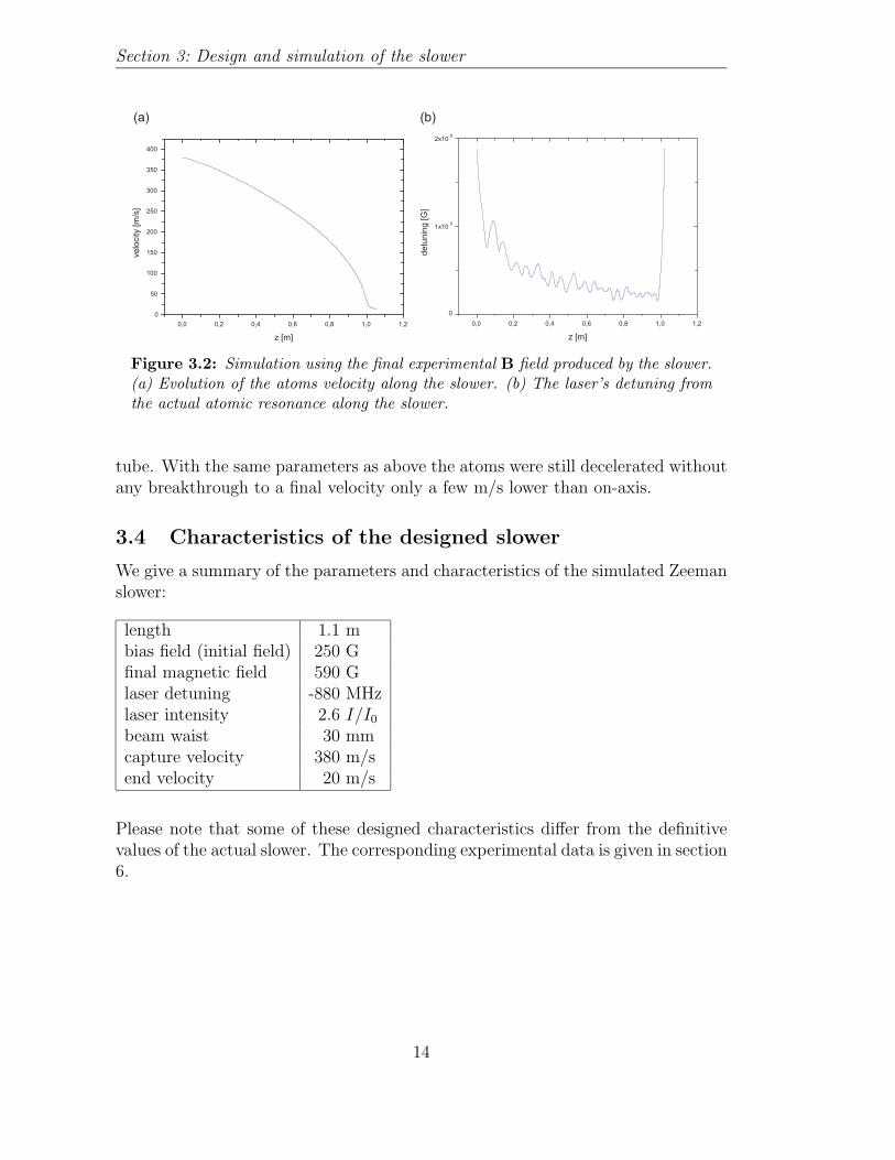
3.3 Simulation of the atoms’ motion

A first test for the designed field profile consisted in the simulation of the atom’smovement inside the Zeeman slower. For this purpose the equation of motion (2.1)was numerically solved, where B(z) specified the detuning δ (eq. (2.14)) in thesaturation parameter given by eq. (2.2).

The slowing laser beam had an initial size of 3 cm diameter at the end of theslower and was focused to 1.5 m away [17]. This provides some transverse coolingfor the atoms and reduces the divergence of the atomic beam [10, 11]. To includethis effect in the simulation, the light intensity was set to

I = I0exp

− 2r2

ω20

[1 +

(λz

πw20

)2]

(1.5 m

z

)2

, (3.4)

where ω0 is such that at z = 1.5 m the beam size is 3 cm (origin of z-axis atslower entrance and z increasing towards slower end). We designed the magneticfield profile for a deceleration a ≈ 2

3amax which requires a laser beam intensity

I/I0 = 2.6 (compare eq. (2.2)). Setting the laser detuning δ0 = −2π · 630 G weadjusted the capture velocity of the atoms to about 380 m/s. The end velocity isthen determined by the difference in the magnetic field between the end and thebeginning of the slower. In our design this value was 340 Gauss, leading to an endvelocity of about 20 m/s.

Fig. 3.2 shows the atoms’ velocity v(z) and the actual detuning δ(z) in functionof their position z. This data was obtained using the real (experimental) magneticfield produced by the solenoid (see section 4) in the simulation. If the criterium(2.17) was not fulfilled at some point, one would see a breakthrough in the plots.The atom would not be decelerated any longer and the detuning would suddenlyrise because the atoms could not follow the magnetic field. Too low light intensityhas the same effect.

To estimate the influence of the higher magnetic field and lower laser intensityoff-axis we also simulated the atoms’ motion 15 mm away from the center of the

13


(a) (b)

0,0 0,2 0,4 0,6 0,8 1,0 1,2 0

50

100

150

200

250

300

350

400

z [m]

velo

city

[m/s

]

0,0 0,2 0,4 0,6 0,8 1,0 1,2

0

1x10 8

2x10 8

z [m]

detu

ning

[G]

Figure 3.2: Simulation using the final experimental B field produced by the slower.(a) Evolution of the atoms velocity along the slower. (b) The laser’s detuning fromthe actual atomic resonance along the slower.

tube. With the same parameters as above the atoms were still decelerated withoutany breakthrough to a final velocity only a few m/s lower than on-axis.

3.4 Characteristics of the designed slower

We give a summary of the parameters and characteristics of the simulated Zeemanslower:

length 1.1 mbias field (initial field) 250 Gfinal magnetic field 590 Glaser detuning -880 MHzlaser intensity 2.6 I/I0

beam waist 30 mmcapture velocity 380 m/send velocity 20 m/s

Please note that some of these designed characteristics differ from the definitivevalues of the actual slower. The corresponding experimental data is given in section6.

14

4 Building the slower

This section describes the practical realization of the Zeeman slower and gives anoverview of the used material.

4.1 The vacuum tube and the wire

A 1.20 m long CF-40 vacuum tube was used to integrate the slower in our vacuumsystem. The inner diameter of 38 mm allows the use of a slowing beam with asufficiently large waist. The efficient magnetic field profile extends over a lengthof 1.1 m which is longer than the minimal requirement (see section 2). This allowsthe field to be less steep which makes the slower less sensitive to field deviations,or — in the perfect case — to increase the capture range. Before winding thesolenoid an electrically isolating spray was applied along the entire vacuum tubeto avoid electric contact to any un-isolated parts of the current carrying wire.

To build the coils producing the bias field a copper tube wire with an inner(outer) diameter of 3 (4) mm was used. This allows water cooling the coils whichwould heat up remarkably with the amount of current we let pass. Since wewanted to implement a bakable Zeeman slower the tube wire was isolated withhigh temperature teflon heat shrink sleeves (Pro Power multicomp STFE4 6.4CLR). The specified shrink factor of 4 was a bit too high for our purpose, so slowand uniform heating in an oven was necessary in order to make the sleeves shrinkthe right amount (i.e. the temperature in the oven was increased with a rate of 1◦C/min).

The coil layers for the tapered field were wound with standard capton-isolated(bakable) copper wire of a diameter of 1.8 mm. Using wire with a squared crosssection would have been advantageous. It prevents the wire loops from slippingbetween the larger copper tubes of the bias layer below. The winding would bemore homogeneous and accurate. This type of wire, however, was not easy toobtain at the time yet.

4.2 Winding the coils

A turning lathe in our workshop facilitated the winding of the coils. The clampedCF-40 tube could be wound just by holding the wire tight while it was turning.An aluminium plate perpendicular to the tube was mounted at its end to alignthe wires at the end of the layers. The two layers for the bias field were builtwith separate tube wires to be able to cool them in parallel. The current circuit,however, was in series. At both ends the coils were provisionally fixed with collarswhich were separated from the layers by a teflon band. Finally, the bias field coilswere covered with a 0.2 mm thick copper sheet, fixed with epoxy to provide aneven ground to wind the remaining coils consisting of thinner wire.

15

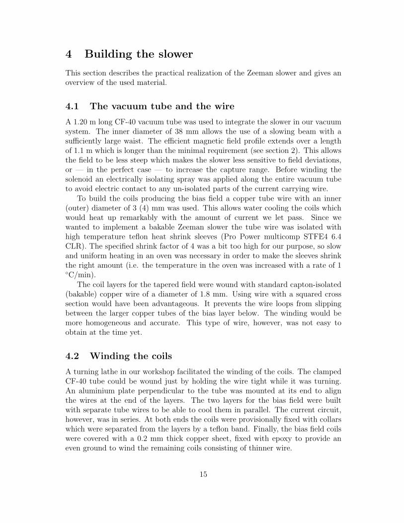
Section 4: Building the slower

radius [mm] positions of layers with quarter, half and full current density [mm]28.9 , , 190, 239 239, 265 265, 304 304, 114330.7 370, 393 412, 491 491, 504 504, 521 521, 545 545, 114332.5 370, 393 , , 412, 491 491, 637 637, 114334.3 , , , 674, 741 741, 800 800, 114336.1 , , , 674, 741 741, 861 861, 114337.9 , , , 881, 919 919, 956 956, 114339.7 , , , 881, 919 919, 998 998, 114341.5 , , , , 1030, 1067 1067, 114343.3 , , , , 1030, 1067 1067, 114345.1 , , , , , 1073, 114346.9 , , , , , 1073, 114348.7 , , , , , 1077, 114350.5 , , , , , 1077, 1143

Table 4.1: Loop radii and (start, end) positions of the coil layers (only biasfield corrected), measured from the outer side of the entrance flange.

Table 4.2 shows the data of the coils producing the tapered magnetic field. Towind the layers with half of the nominal current density a second wire was woundat the same time, keeping the correct spacing between the current carrying loops.All layers consist of one single piece of wire. Therefore the winding helicity of a coilwould be opposite to the one of the layer underneath it. At some places the wirewould then slip into the gap between two wires below, resulting in an irregular andtotally reduced loop density. By adjusting the remaining layers in the simulationappropriately we could correct these errors. Finally, another series of correctionloops was added after measuring the total field produced as described below. Thepositions and current densities of the those layers are summarized in table 4.2.The thin wire was provisionally fixed with cable ties which later were replaced bywire straps. A way around the irregular slipping problem would be to use wirewith a squared cross section.

radius [mm] positions of layers with full and third current density [mm]28.9 125, 150 25, 75 , ,30.7 230, 239 283, 298 , ,34.3 375, 385 455, 475 530, 541 605, 65537.9 715, 720 790, 800 832, 845 ,41.5 893, 910 953, 970 1005, 1035 ,45.1 1035, 1050 , , ,

Table 4.2: Loop radii and (start, end) positions of the additional correctionlayers, measured from the outer side of the entrance flange.

16


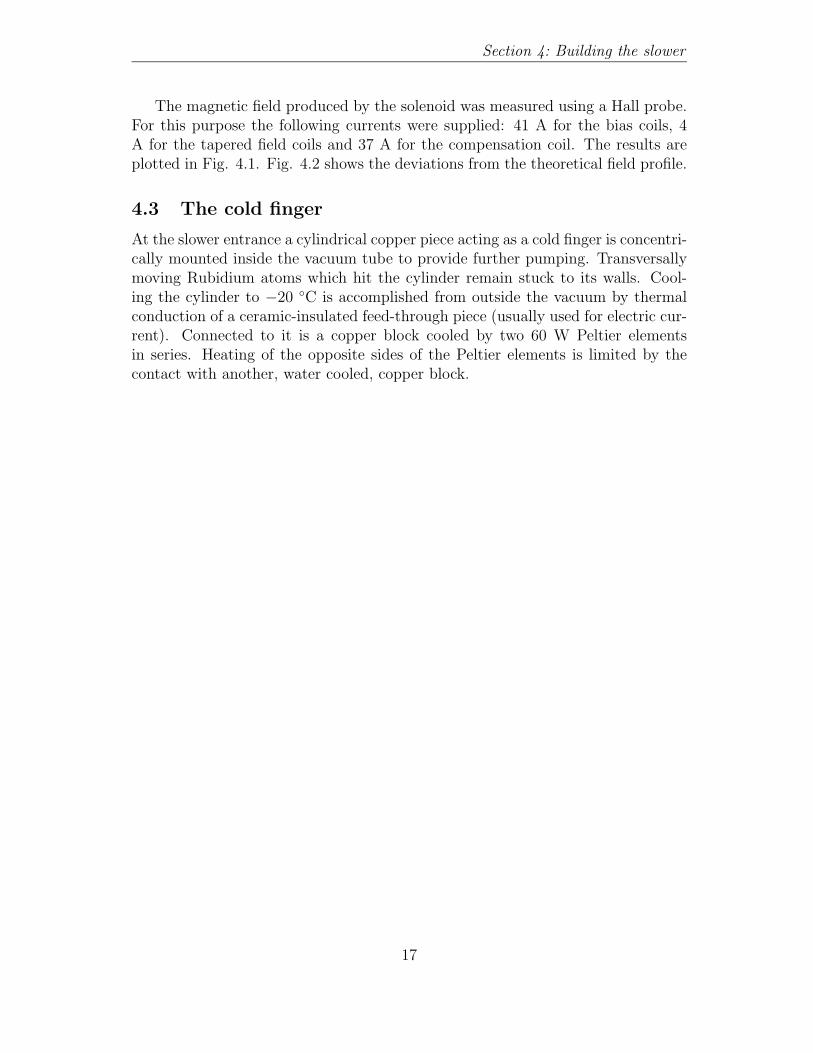
The magnetic field produced by the solenoid was measured using a Hall probe.For this purpose the following currents were supplied: 41 A for the bias coils, 4A for the tapered field coils and 37 A for the compensation coil. The results areplotted in Fig. 4.1. Fig. 4.2 shows the deviations from the theoretical field profile.

4.3 The cold finger

At the slower entrance a cylindrical copper piece acting as a cold finger is concentri-cally mounted inside the vacuum tube to provide further pumping. Transversallymoving Rubidium atoms which hit the cylinder remain stuck to its walls. Cool-ing the cylinder to −20 ◦C is accomplished from outside the vacuum by thermalconduction of a ceramic-insulated feed-through piece (usually used for electric cur-rent). Connected to it is a copper block cooled by two 60 W Peltier elementsin series. Heating of the opposite sides of the Peltier elements is limited by thecontact with another, water cooled, copper block.

17


0,0 0,2 0,4 0,6 0,8 1,00

50

100

150

200

250

300

350

400

450

500

550

B [G

]

z [m]

bias field uncorrected field corrected field without compensation corrected field with compensation

Figure 4.1: Measured magnetic fields of the Zeeman slower before andafter corrections.

0,0 0,2 0,4 0,6 0,8 1,0 1,2

-5

0

5

B [G

]

z [m]

deviation from optimal field profile allowed error range

Figure 4.2: Deviations of the measured magnetic field from the theo-retical profile. The errors are within the range as discussed in section3.

18

5 The (recirculating) Rubidium oven

With the implementation of a Zeeman slower in our experimental setup we alsointroduced a new Rubidium source to provide a high load of atoms. This sectiondescribes the recirculating oven which replaces the former room temperature gaschamber. To get more insight into the subject of atomic beam sources, pleaseconsult the references [18] and [19].

5.1 The setup

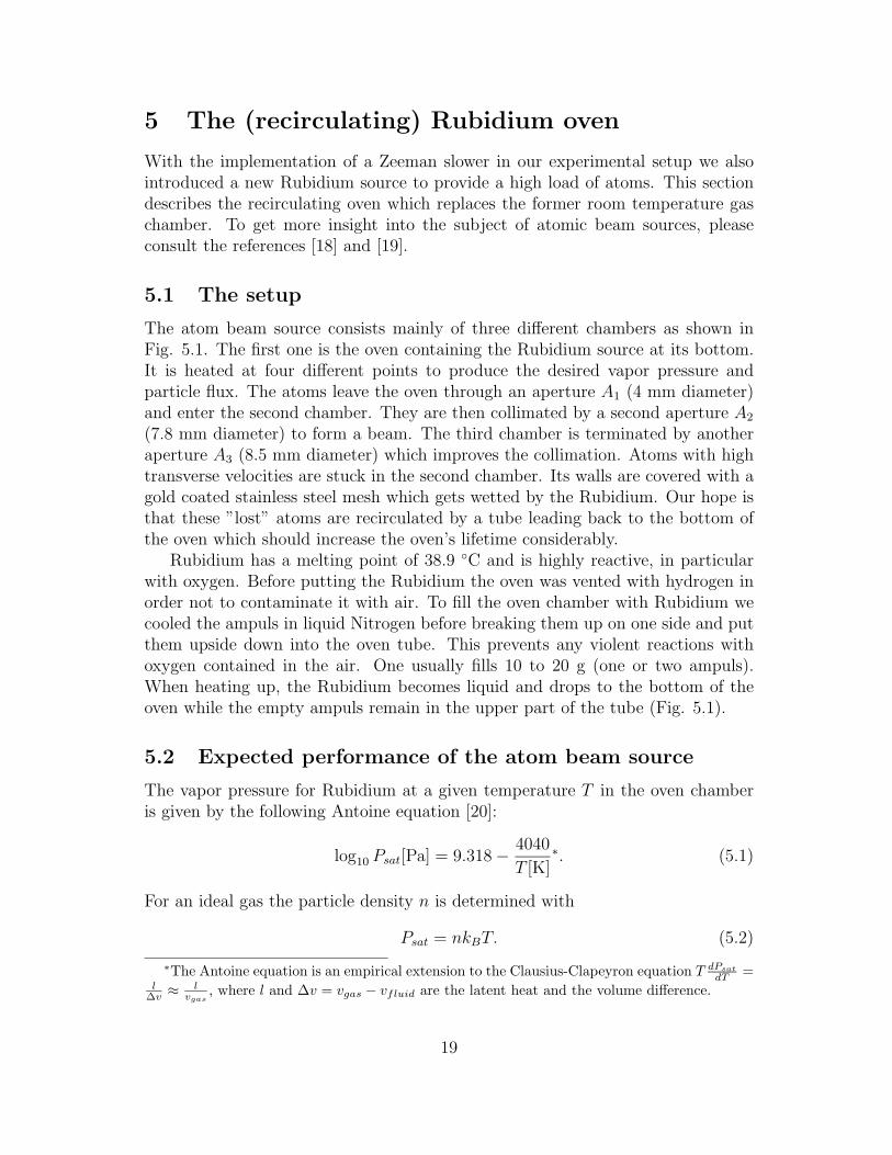
The atom beam source consists mainly of three different chambers as shown inFig. 5.1. The first one is the oven containing the Rubidium source at its bottom.It is heated at four different points to produce the desired vapor pressure andparticle flux. The atoms leave the oven through an aperture A1 (4 mm diameter)and enter the second chamber. They are then collimated by a second aperture A2

(7.8 mm diameter) to form a beam. The third chamber is terminated by anotheraperture A3 (8.5 mm diameter) which improves the collimation. Atoms with hightransverse velocities are stuck in the second chamber. Its walls are covered with agold coated stainless steel mesh which gets wetted by the Rubidium. Our hope isthat these ”lost” atoms are recirculated by a tube leading back to the bottom ofthe oven which should increase the oven’s lifetime considerably.

Rubidium has a melting point of 38.9 ◦C and is highly reactive, in particularwith oxygen. Before putting the Rubidium the oven was vented with hydrogen inorder not to contaminate it with air. To fill the oven chamber with Rubidium wecooled the ampuls in liquid Nitrogen before breaking them up on one side and putthem upside down into the oven tube. This prevents any violent reactions withoxygen contained in the air. One usually fills 10 to 20 g (one or two ampuls).When heating up, the Rubidium becomes liquid and drops to the bottom of theoven while the empty ampuls remain in the upper part of the tube (Fig. 5.1).

5.2 Expected performance of the atom beam source

The vapor pressure for Rubidium at a given temperature T in the oven chamberis given by the following Antoine equation [20]:

log10 Psat[Pa] = 9.318 − 4040

T [K]∗. (5.1)

For an ideal gas the particle density n is determined with

Psat = nkBT. (5.2)

∗The Antoine equation is an empirical extension to the Clausius-Clapeyron equation T dPsat

dT =l

∆v ≈ lvgas

, where l and ∆v = vgas − vfluid are the latent heat and the volume difference.

19

Section 5: The (recirculating) Rubidium oven

4 mm

4 mm 7.8 mm 8.5 mm

6 mm

79 mm

125 mm

ion pump

Rb beam

T3

T2

T4

T1 15 g Rb

Peltier

recirculating tube

oven chamber

Figure 5.1: The atomic beam source, consisting of a re-circulating oven and collimators, and its dimensions. ThePeltier element serves as an additional Rb pump.

To illustrate the importance of the recirculation we compare the particle fluxout of the oven chamber with the one after the collimation. The derivation of thesequantities is done in appendix A. The results are as follows (notation as in Fig.5.1):

Φ0 =1

4nA1v, (5.3)

the flux out of the oven chamber, and

Φc =nA1A3v

4πd2, (5.4)

the flux of the collimated beam. Both depend directly on the oven temperaturethrough v = (8kBT

πm)1/2. In our setup the distance between A1 and A3 is d = 20.4

cm, so the atomic beam only contains Φc/Φ0 = A3/πd2 ≈ 0.2% of the atoms thatleave the oven. In other words, recirculation can in principle increase the oven’slifetime by a factor 500.

20


Temperature [ C] Pressure [Pa] Pressure[Torr] Density [m-3] Beam velocity [m/s] Flux of 87Rb [at/s] Lifetime of 1g [h]

100 3,10E-02 2,33E-04 6,02E+18 356 8,17E+11 338

110 5,94E-02 4,47E-04 1,12E+19 360 1,55E+12 179

120 1,10E-01 8,28E-04 2,03E+19 365 2,83E+12 98

130 1,98E-01 1,49E-03 3,56E+19 370 5,03E+12 55

140 3,46E-01 2,60E-03 6,07E+19 374 8,68E+12 32

150 5,90E-01 4,43E-03 1,01E+20 379 1,46E+13 19

160 9,79E-01 7,36E-03 1,64E+20 383 2,40E+13 12

170 1,59E+00 1,20E-02 2,60E+20 387 3,85E+13 7

180 2,53E+00 1,90E-02 4,04E+20 392 6,05E+13 5

190 3,94E+00 2,96E-02 6,16E+20 396 9,32E+13 3

200 6,02E+00 4,53E-02 9,22E+20 400 1,41E+14 2

210 9,04E+00 6,80E-02 1,36E+21 405 2,09E+14 1

220 1,34E+01 1,00E-01 1,96E+21 409 3,06E+14 1

230 1,94E+01 1,46E-01 2,80E+21 413 4,41E+14 1

240 2,79E+01 2,10E-01 3,93E+21 417 6,27E+14 0

250 3,94E+01 2,96E-01 5,46E+21 421 8,77E+14 0

260 5,50E+01 4,14E-01 7,48E+21 425 1,21E+15 0

270 7,58E+01 5,70E-01 1,01E+22 429 1,66E+15 0

280 1,03E+02 7,77E-01 1,35E+22 433 2,24E+15 0

290 1,39E+02 1,05E+00 1,79E+22 437 2,99E+15 0

300 1,86E+02 1,40E+00 2,35E+22 441 3,95E+15 0

Pressure, density and flux for rubidium in function of T

Table 5.1: Calculated data for our Rubidium source(85Rb and 87Rb). Theflux after collimation is given. Note that the indicated oven lifetime is validfor a non-recirculating oven.

5.3 Temperature control

From eq. (5.2) and (5.3) we deduce Φ ∼ Psat

T. Table 5.1 lists oven pressure, density,

velocity, flux and lifetime in function of the temperature. While a conventionaloven at usual operating condition has a lifetime of about 800 hours, our oven —if it recirculates — is expected to operate for at least one year without refilling ofRubidium.

To control the atomic flux out of our oven, we use four heating tapes, ther-mocouplers and PID temperature controllers (Omega CN1166-DC1). Thermalisolation is improved by a fiber glass cord wound around the oven chamber. Theoven temperature T1 is typically kept between 120 and 160 ◦C, whereas the re-maining three heating points T2, T3 and T4 are 30 ◦C above the value of T1 (Fig.5.1). This prevents the Rubidium from sticking to the oven walls.

21


22

6 Testing and characterization

In the following paragraphs I describe our experimental setup to test and charac-terize the Zeeman slower and present the results of our measurements.

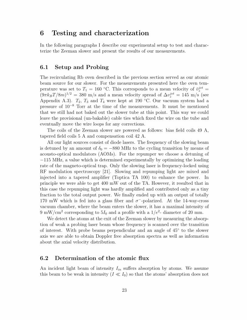
6.1 Setup and Probing

The recirculating Rb oven described in the previous section served as our atomicbeam source for our slower. For the measurements presented here the oven tem-perature was set to T1 = 160 ◦C. This corresponds to a mean velocity of vjet

z =(9πkBT/8m)1/2 = 380 m/s and a mean velocity spread of ∆vjet

z = 145 m/s (seeAppendix A.3). T2, T3 and T4 were kept at 190 ◦C. Our vacuum system had apressure of 10−8 Torr at the time of the measurements. It must be mentionedthat we still had not baked out the slower tube at this point. This way we couldleave the provisional (un-bakable) cable ties which fixed the wire on the tube andeventually move the wire loops for any corrections.

The coils of the Zeeman slower are powered as follows: bias field coils 49 A,tapered field coils 5 A and compensation coil 42 A.

All our light sources consist of diode lasers. The frequency of the slowing beamis detuned by an amount of δ0 = −880 MHz to the cycling transition by means ofacousto-optical modulators (AOMs). For the repumper we choose a detuning of−115 MHz, a value which is determined experimentally by optimizing the loadingrate of the magneto-optical trap. Only the slowing laser is frequency-locked usingRF modulation spectroscopy [21]. Slowing and repumping light are mixed andinjected into a tapered amplifier (Toptica TA 100) to enhance the power. Inprinciple we were able to get 400 mW out of the TA. However, it resulted that inthis case the repumping light was hardly amplified and contributed only as a tinyfraction to the total output power. We finally ended up with an output of totally170 mW which is fed into a glass fiber and σ−-polarized. At the 14-way-crossvacuum chamber, where the beam enters the slower, it has a maximal intensity of9 mW/cm2 corresponding to 5I0 and a profile with a 1/e2- diameter of 20 mm.

We detect the atoms at the exit of the Zeeman slower by measuring the absorp-tion of weak a probing laser beam whose frequency is scanned over the transitionof interest. With probe beams perpendicular and an angle of 45◦ to the sloweraxis we are able to obtain Doppler free absorption spectra as well as informationabout the axial velocity distribution.

6.2 Determination of the atomic flux

An incident light beam of intensity Iin suffers absorption by atoms. We assumethis beam to be weak in intensity (I I0) so that the atoms’ absorption does not

23

Section 6: Testing and characterization

⊗

�T1 •

T2 •

T3 •

•T4

Rb (15 g)

oven

recirculation tube

gate valve

ion pump

slowing

titanium pump

slowinglight

bias field coils

tapered field coils

PeltierPeltier

compensation coil

14-way-cross

probe beams

ion pump

A1 A2 A3

Figure 6.1: Experimental setup to test the Zeeman slower. The slowed atomsare probed in a 14-way-cross vacuum chamber which will later serve as a cham-ber for the 2D-MOT.

saturate. The transmitted intensity Itr is then given by

Itr = IinT = Iine− ∫ ∞

−∞ n(x)σdx, (6.1)

where n(x) is the particle density per unit volume at a location x and σ the crosssection. The integral is to be taken along the path of the laser beam. The opticaldensity is defined as the negative exponent of the transmission coefficient T :

D = − log T =

∫ ∞

−∞n(x)σdx ≈ nσl. (6.2)

The approximation is valid when the density n does not vary a lot over the distancel where the beam interacts with the atoms. The flux of an atomic beam with meanvelocity v reads

Φ = nπl2

4v =

πl

4σDv. (6.3)

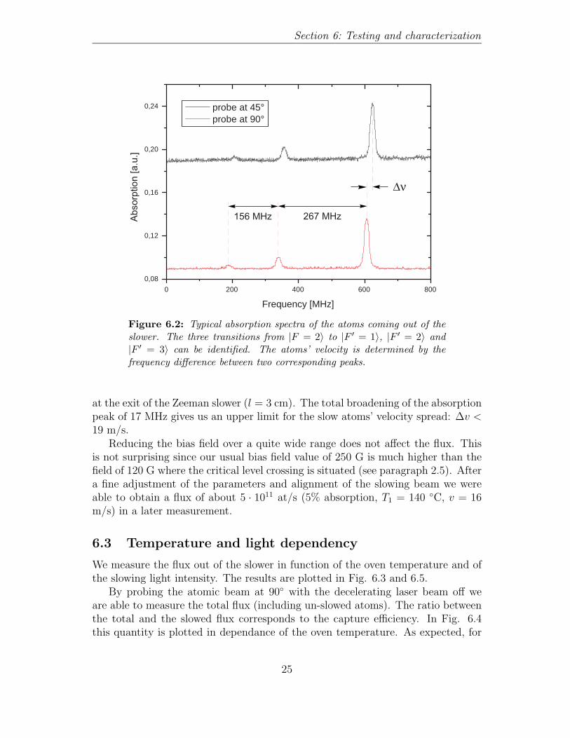
The cross section for scattering resonant light of wavelength λ is given by σ ≈λ2/2π (cycling transition, linear polarization). By measuring the absorption onecan calculate the optical density and determine the atomic flux. Absorption peaksof a gas usually show various enlargement effects, as Doppler or power broadening,which have to be taken into account. Given that the number of detected atomsis not changed, the surface below the absorption peak with or without broadeningeffects is the same. Thus, as an approximation the ratio of the height of the un-broadened absorption peak to the broadened one is the inverse of the ratio of theirfull widths of half maximum, ∆ν/Γ with Γ = 5.9 MHz.

The absorption profile obtained with the 45◦ probe is plotted in Fig. 6.2. Wemeasured an absorption of 1 − T = 1.27% at a frequency shifted by ∆ν45◦ = 20MHz with respect to the Doppler free spectrum. The velocity of the slowed beamis given by v = λ∆ν45◦/ cos 45◦ = 22 m/s. This corresponds to an atomic flux of

Φ = 1.8 · 1011at/s (6.4)

24


0 200 400 600 800

0,08

0,12

0,16

0,20

0,24

Frequency [MHz]

probe at 45° probe at 90°

156 MHz 267 MHz

∆ν

Abs

orpt

ion

[a.u

.]

Figure 6.2: Typical absorption spectra of the atoms coming out of theslower. The three transitions from |F = 2〉 to |F ′ = 1〉, |F ′ = 2〉 and|F ′ = 3〉 can be identified. The atoms’ velocity is determined by thefrequency difference between two corresponding peaks.

at the exit of the Zeeman slower (l = 3 cm). The total broadening of the absorptionpeak of 17 MHz gives us an upper limit for the slow atoms’ velocity spread: ∆v <19 m/s.

Reducing the bias field over a quite wide range does not affect the flux. Thisis not surprising since our usual bias field value of 250 G is much higher than thefield of 120 G where the critical level crossing is situated (see paragraph 2.5). Aftera fine adjustment of the parameters and alignment of the slowing beam we wereable to obtain a flux of about 5 · 1011 at/s (5% absorption, T1 = 140 ◦C, v = 16m/s) in a later measurement.

6.3 Temperature and light dependency

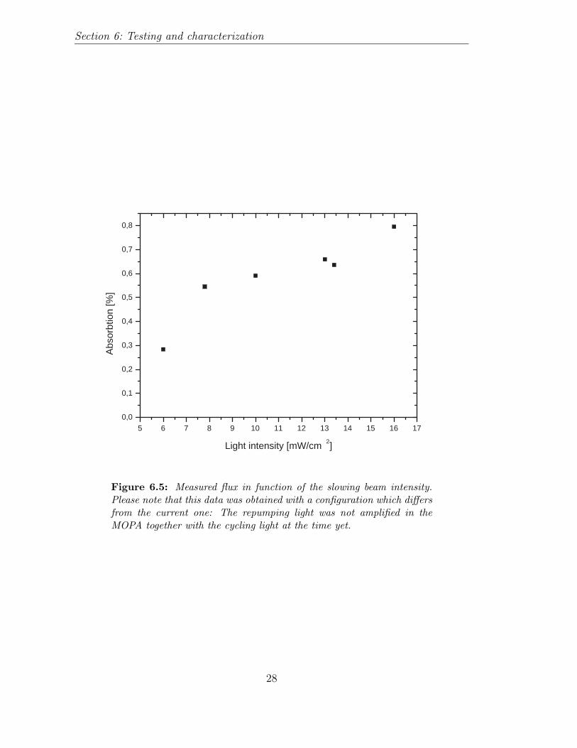
We measure the flux out of the slower in function of the oven temperature and ofthe slowing light intensity. The results are plotted in Fig. 6.3 and 6.5.

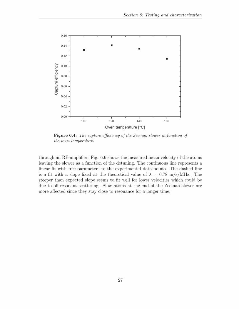
By probing the atomic beam at 90◦ with the decelerating laser beam off weare able to measure the total flux (including un-slowed atoms). The ratio betweenthe total and the slowed flux corresponds to the capture efficiency. In Fig. 6.4this quantity is plotted in dependance of the oven temperature. As expected, for

25


60 80 100 120 140 160

10 10

10 11

10 12

Oven temperature [°C]

total (slowed and un-decelerated) slowed, probe at 45° slowed, probe at 90°

Flu

x [a

tom

s/s]

Figure 6.3: Measured fluxes in function of the oven temperature.

high temperatures the capture efficiency decreases slightly because of the chang-ing velocity distribution of the atoms. According to eq. (A.10) of the appendixthe portion of atoms with a velocity below the capture velocity of the slower iscalculated as:

pcapt =

∫ vcapt

0dvzv

3z exp(− mv2

z

2kBT)∫ ∞

0dvzv3

z exp(− mv2z

2kBT)

. (6.5)

For vcapt = 380 m/s this quantity varies between 66% and 52% for an oven tem-perature between 60 ◦C and 160 ◦C. The measured capture efficiency as plotted inFig. 6.4 varies slowly around a value of 13%. This result is quite satisfying consid-ering the additional atom loss due to transverse heating (see paragraph 2.2). Slightchanges in the polarization of the slowing beam did not show remarkable effects.Also, the slower works well without repumping light (see section 2), although ithelps as one sees when optimizing its frequency detuning for the MOT loading.

6.4 Final velocity of the slowed atoms

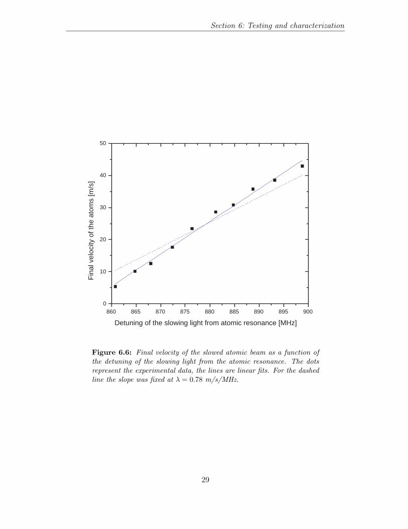
The slowing laser beam is detuned from the atomic resonance by means of anacousto-optical modulator (AOM). The frequency offset is adjusted by chang-ing the voltage of the voltage-controlled oscillator (VCO) which drives the AOM

26


100 120 140 160

0,00

0,02

0,04

0,06

0,08

0,10

0,12

0,14

0,16

Oven temperature [°C]

Cap

ture

effi

cien

cy

Figure 6.4: The capture efficiency of the Zeeman slower in function ofthe oven temperature.

through an RF-amplifier. Fig. 6.6 shows the measured mean velocity of the atomsleaving the slower as a function of the detuning. The continuous line represents alinear fit with free parameters to the experimental data points. The dashed lineis a fit with a slope fixed at the theoretical value of λ = 0.78 m/s/MHz. Thesteeper than expected slope seems to fit well for lower velocities which could bedue to off-resonant scattering. Slow atoms at the end of the Zeeman slower aremore affected since they stay close to resonance for a longer time.

27


5 6 7 8 9 10 11 12 13 14 15 16 170,0

0,1

0,2

0,3

0,4

0,5

0,6

0,7

0,8

Abs

orbt

ion

[%]

Light intensity [mW/cm 2]

Figure 6.5: Measured flux in function of the slowing beam intensity.Please note that this data was obtained with a configuration which differsfrom the current one: The repumping light was not amplified in theMOPA together with the cycling light at the time yet.

28


860 865 870 875 880 885 890 895 9000

10

20

30

40

50

Fin

al v

eloc

ity o

f the

ato

ms

[m/s

]

Detuning of the slowing light from atomic resonance [MHz]

Figure 6.6: Final velocity of the slowed atomic beam as a function ofthe detuning of the slowing light from the atomic resonance. The dotsrepresent the experimental data, the lines are linear fits. For the dashedline the slope was fixed at λ = 0.78 m/s/MHz.

29


30

7 Summary and Conclusions

In this article I have described the theory, design and building of a Zeeman slowerfor 87Rb.

The implemented increasing field slower shows excellent performance. It pro-vides a flux of the order of 1011 at/s at a final velocity of the order of 10 m/swhich allows to load efficiently our magneto-optical trap. Together with the new(recirculating) oven, we have thus implemented an outstanding atomic source toinject the magnetic guide. Compared with the old setup, this makes the currentstatus of the atom laser experiment very promising. Indeed, evidence for collisionsbetween the atoms in the guide has been detected recently.

31

Section A: Particle flux and mean velocity of an atomic beam

A Particle flux and mean velocity of an atomic

beam

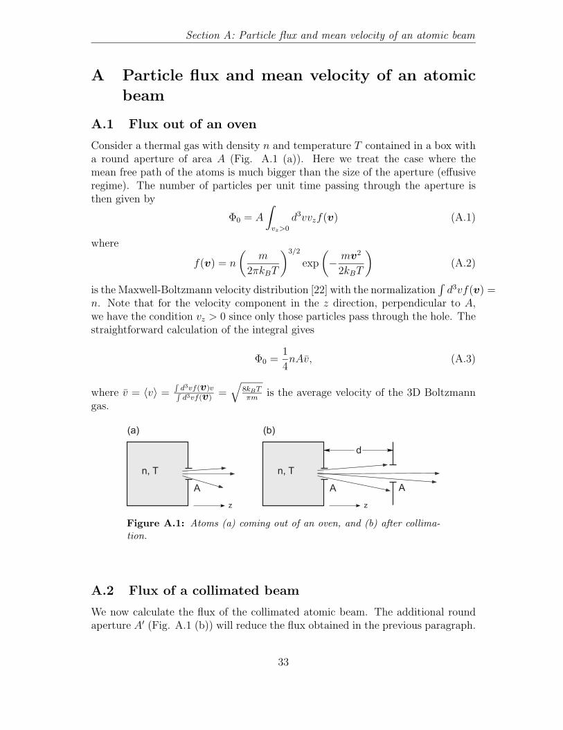
A.1 Flux out of an oven

Consider a thermal gas with density n and temperature T contained in a box witha round aperture of area A (Fig. A.1 (a)). Here we treat the case where themean free path of the atoms is much bigger than the size of the aperture (effusiveregime). The number of particles per unit time passing through the aperture isthen given by

Φ0 = A

∫vz>0

d3vvzf(v) (A.1)

where

f(v) = n

(m

2πkBT

)3/2

exp

(− mv2

2kBT

)(A.2)

is the Maxwell-Boltzmann velocity distribution [22] with the normalization∫

d3vf(v) =n. Note that for the velocity component in the z direction, perpendicular to A,we have the condition vz > 0 since only those particles pass through the hole. Thestraightforward calculation of the integral gives

Φ0 =1

4nAv, (A.3)

where v = 〈v〉 =∫

d3vf(v)v∫d3vf(v)

=√

8kBTπm

is the average velocity of the 3D Boltzmanngas.

A

n, T

A

n, Tn, T

A

z

A

z

(a) (b)

d

Figure A.1: Atoms (a) coming out of an oven, and (b) after collima-tion.

A.2 Flux of a collimated beam

We now calculate the flux of the collimated atomic beam. The additional roundaperture A′ (Fig. A.1 (b)) will reduce the flux obtained in the previous paragraph.

33

Section A: Particle flux and mean velocity of an atomic beam

The transverse velocity components (parallel to the area A′) are limited by thecondition v⊥/vz < (A′/πd2)1/2, where d is the distance between the apertures Aand A′. We thus calculate the integral

Φc = A

∫vz>0,v⊥<vz( A′

πd2 )12

d3vvzf(v) =1

4nA

A′

A′ + πd2v. (A.4)

Since A′ πd2 the flux of the atomic beam after collimation reads

Φc ≈ nAA′v4πd2

. (A.5)

A.3 Mean velocity of an atomic beam

Whereas the number of particles contained in a box is conserved, in the case of abeam it depends linearly on time. Consider a collimated particle beam as in theprevious paragraph. The number of particles having a velocity between vz andvz + dvz in the beam at a time t (at t = 0 the aperture A is opened) is given by

dN = Avztf(vz)dvz, (A.6)

where f(vz) is the Maxwell-Boltzmann distribution f(v) integrated over the trans-verse velocity components v⊥ as above. The average velocity in the direction ofthe beam z is thus calculated as

vjetz ≡ 〈vz〉jet =

∫ ∞0

dNvz∫ ∞0

dN=

∫ ∞0

dvzf(vz)v2z∫ ∞

0dvzf(vz)vz

. (A.7)

Applying again the approximation A′ πd2 one receives

vjetz ≈

√9πkBT

8m. (A.8)

We also calculate the standard deviation from this mean value,

∆vjetz =

√〈v2

z〉jet − (〈vz〉jet)2 = ∆vjetz ≈

√2kBT

m

(2 − 9

16π

). (A.9)

Note that in the above approximation one finds the dependence f(vz) ∝ v2z exp(− mv2

z

2kBT)

for the longitudinal velocity distribution. In general, the mean value of a quan-tity B(vz) depending only on the longitudinal velocity component is thus simplycalculated as

〈B(vz)〉 =

∫ ∞0

dvzB(vz)f(vz)vz∫ ∞0

dvzf(vz)vz

=

∫ ∞0

dvzB(vz)v3z exp(− mv2

z

2kBT)∫ ∞

0dvzv3

z exp(− mv2z

2kBT)

. (A.10)

34

References

[1] A. P. Chikkatur et al., Science 296, 2193-2195 (2002).

[2] E. Mandonnet et al., Eur. Phys. J. D 10, 9-18 (2000).

[3] E. L. Raab et al., Phys. Rev. Lett. 59, 2631 (1987).

[4] P. Cren et al. Eur., Phys. J. D 20, 107-116 (2002).

[5] W. D. Phillips, J. V. Prodan, H. J. Metcalf, J. Opt. Soc. Am. B2, 11 (1985).

[6] A. Scholz et al., Opt. Comm. 111, 155-162 (1994).

[7] W. Ertmer et al., Phys. Rev. Lett. 54, 996-999 (1985).

[8] J. Hoffnagle. Opt. Lett. 13, 92 (1988).

[9] M. Zhu et al., Phys. Rev. Lett. 67, 46-49 (1991).

[10] H. J. Metcalf, P. van der Straaten, Laser Cooling and Trapping. Springer 1999.

[11] M. A. Joffe et al., J. Opt. Soc. Am. B 10, 12 (1993).

[12] B. H. Bransden, C.J. Joachain, Physics of Atoms and Molecules. PrenticeHall, second edition.

[13] R. J. Napolitano et al. Opt. Comm. 80, 110 (1990).

[14] W. D. Phillips, H. Metcalf. Phys. Rev. Lett. 48, 9 (1982).

[15] T. E. Barrett et al., Phys. Rev. Lett. 67, 25 (1991).

[16] J. D. Jackson, Classical Electrodynamics. Wiley, third edition, 1998.

[17] P. A Molenaar et al., Phys. Rev. A 55, 605 (1997).

[18] L. Vestergaard Hau, J. A. Golovchenko, Rev. Sci. Instrum. 65 , 12 (1994).

[19] M. R. Walkiewicz et al., Rev. Sci. Instrum. 71, 3342 (2000).

[20] Handbook of Chemistry and Physics. CRC Press, 84th edition, 2003-2004.

[21] W. Demtroder.Laserspektroskopie, Grundlagen und Techniken. Springer, 4.Auflage, 2000.

[22] K. Huang, Statistical Mechanics. Wiley, second edition, 1987.

35

Literature

36

Acknowledgement

The work presented in this report was part of the first year of my PhD thesis.I had the great opportunity to spend that time in Jean Dalibard’s and DavidGuery-Odelin’s group in Paris. I am very grateful to Jean and David for havingmade possible my stay in the Laboratoire Kastler-Brossel. It was a great scientificexperience in a very friendly athmosphere. Also, David was so kind to read thisreport carefully.

Furthermore, I’d like to thank Thierry Lahaye, the other PhD student of thegroup. His careful working style is amazing. Thanks also go to Johnny Vogels whohelped me in the careful design and the realization of the Zeeman slower. Alsoinvolved in the practical work was Leticia Tarruel whom I’d like to thank for herassistance during her internship.

My work was supported by a Marie-Curie Fellowship (QPAF).

37

design and implementation of a zeeman slower for … · design and implementation of a zeeman...

Documents