design and experimental realization of adaptive control...

Design and Experimental Realization of Adaptive

Control Schemes for an Autonomous Underwater

Vehicle

Dissertation submitted in partial fulfillment

of the requirements of the degree of

Doctor of Philosophy

in

Electrical Engineering

by

Raja Rout

(512EE104)

based on research carried out

under the supervision of

Prof. Bidyadhar Subudhi

DEPARTMENT OF ELECTRICAL ENGINEERING

NATIONAL INSTITUTE OF TECHNOLOGY ROURKELA

JANUARY 2017

CERTIFICATE OF EXAMINATION

09/01/2017

Roll Number : 512EE104

Name: Raja Rout

Title of Dissertation: Design and Experimental Realization of Adaptive Control

Schemes for an Autonomous Underwater Vehicle

We the below signed, after checking the dissertation mentioned above and the official

record book(s) of the student, hereby state our approval of the dissertation submitted

in partial fulfillment of the requirements of the degree of Doctor of Philosophy in

Electrical Engineering at National Institute of Technology Rourkela. We are satisfied

with the volume, quality, correctness, and originality of the work.

Prof. D. R. K. Parhi

(Member, DSC)

Prof. U. C. Pati

(Member, DSC)

Prof. A. K. Naskar

(Member, DSC)

Prof. A. K. Panda

(Chairperson, DSC)

Prof. B. Subudhi

(Supervisor)

Prof. A. Gupta

(External Examiner)

Prof. J. K. Satapathy

(Head of the Department)

CERTIFICATE

This is to certify that the work presented in the dissertation entitled “Design and

Experimental Realization of Adaptive Control Schemes for an Autonomous

Underwater Vehicle” submitted by Raja Rout, Roll Number 512EE104, is a record

of original research carried out by him under my supervision and guidance in partial

fulfillment of the requirements of the degree of Doctor of Philosophy in Electrical En-

gineering. Neither this dissertation nor any part of it has been submitted earlier for

any degree or diploma to any institute or university in India or abroad.

Prof. Bidyadhar Subudhi

(Supervisor)

Declaration of Originality

I, Raja Rout, Roll Number 512EE104 hereby declare that this dissertation entitled

“Design and Experimental Realization of Adaptive Control Schemes for

an Autonomous Underwater Vehicle” presents my original work carried out as

a doctoral student of NIT Rourkela and, to the best of my knowledge, contains no

material previously published or written by another person, nor any material presented

by me for the award of any degree or diploma of NIT Rourkela or any other institution.

Any contribution made to this research by others, with whom I have worked at NIT

Rourkela or elsewhere, is explicitly acknowledged in the dissertation. Works of other

authors cited in this dissertation have been duly acknowledged under the sections

Reference or Bibliography. I have also submitted my original research records to the

scrutiny committee for evaluation of my dissertation.

I am fully aware that in case of any non-compliance detected in future, the Senate

of NIT Rourkela may withdraw the degree awarded to me on the basis of the present

dissertation.

RAJA ROUT

ACKNOWLEDGEMENTS

First and foremost, I am truly indebted to my supervisor Prof. Bidyadhar Subudhi

for his guidance and unwavering confidence through my study, without which this

thesis would not be in its present form. I also thank him for gracious encouragement

throughout the work.

I express my sincere gratitude to the Doctoral Scrutiny Committee chairman Prof.

A. K. Panda and its members Prof. D. R. K. Parhi, Prof. U. C. Pati, Prof. A.

K. Naskar for their suggestion to improve the work. I am also very much obliged to

Head of the Department of Electrical Engineering, Prof. J. K. Satapathy for providing

possible facilities. I also express my earnest thanks to Prof. Sandip Ghosh for his

valuable suggestion and thanks to other faculty members in the department. I would

also like to thank Sahadev Swain and Budu Oram for their assistance during my stay

at Control and Robotics laboratory.

I would especially like to thank my colleague Subhasish, for his support in develop-

ing the AUV. I also thank to Biranchi, Chhavi and Shivam for their enjoyable moment

during experimental tests at swimming pool. I thank to my seniors Dushmanta Ku.

Dash, Shantanu Pradhan, Basant Ku. Sahu, Sathyam Bonala, Srinibas Bhuyan and

Raseswari Pradhan for their inspiration and suggestion which helped me to complete

this thesis.

My wholehearted gratitude to my beloved parents Smt. Promodini Rout and Sri.

Ashok Kumar Rout for their encouragement and support. Thank you for believing in

me.

RAJA ROUT

Abstract

Research on Autonomous Underwater Vehicle(AUV) has attracted increased attention

of control engineering community in the recent years due to its many interesting appli-

cations such as in Defense organisations for underwater mine detection, region surveil-

lance, oceanography studies, oil/gas industries for inspection of underwater pipelines

and other marine related industries. However, for the realization of these applications,

effective motion control algorithms need to be developed. These motion control algo-

rithms require mathematical representation of AUV which comprises of hydrodynamic

damping, Coriolis terms, mass and inertia terms etc. To obtain dynamics of an AUV,

different analytical and empirical methods are reported in the literature such as tow

tank test, Computational Fluid Dynamics (CFD) analysis and on-line system identi-

fication. Among these methods, tow-tank test and CFD analysis provide white-box

identified model of the AUV dynamics. Thus, the control design using these methods

are found to be ineffective in situation of change in payloads of an AUV or parametric

variations in AUV dynamics. On the other hand, control design using on-line identi-

fication, the dynamics of AUV can be obtained at every sampling time and thus the

aforesaid parametric variations in AUV dynamics can be handled effectively.

In this thesis, adaptive control strategies are developed using the parameters of

AUV obtained through on-line system identification. The proposed algorithms are

verified first through simulation and then through experimentation on the prototype

AUV. Among various motion control algorithms, waypoint tracking has more practi-

cal significance for oceanographic surveys and many other applications. In order to

ii

implement, waypoint motion control schemes, Line-of-Sight (LoS) guidance law can be

used which is computationally less expensive. In this thesis, adaptive control schemes

are developed to implement LoS guidance for an AUV for practical realization of the

control algorithm.

Further, in order to realize the proposed control algorithms, a prototype AUV is

developed in the laboratory. The developed AUV is a torpedo-shaped in order to ex-

perience low drag force, underactuated AUV with a single thruster for forward motion

and control planes for angular motion. Firstly, the AUV structure such as nose profile,

tail profile, hull section and control planes are designed and developed. Secondly, the

hardware configuration of the AUV such as sensors, actuators, computational unit,

communication module etc. are appropriately selected. Finally, a software frame-

work called Robot Operating System (ROS) is used for seamless integration of various

sensors, actuators with the computational unit. ROS is a software platform which

provides right platform for the implementation of the control algorithms using the

sensor data to achieve autonomous capability of the AUV.

In order to develop adaptive control strategies, the unknown dynamics of the AUV

is identified using polynomial-based Nonlinear Autoregressive Moving Average eXoge-

nous (NARMAX) model structure. The parameters of this NARMAX model structure

are identified online using Recursive Extended Least Square (RELS) method. Then an

adaptive controller is developed for realization of the LoS guidance law for an AUV.

Using the kinematic equation and the desired path parameters, a Lyapunov based

backstepping controller is designed to obtain the reference velocities for the dynam-

ics. Subsequently, a self-tuning PID controller is designed for the AUV to track these

reference velocities. Using an inverse optimal control technique, the gains of the self-

tuning PID controller are tuned on-line. Although, this algorithm is computationally

less expensive but there lie issues such as actuator constraints and state constraints

which need to be resolved in view of practical realization of the control law. It is also

observed that the proposed NARMAX structure of the AUV consists of redundant

iii

regressor terms.

To alleviate the aforesaid limitations of the Inverse optimal self-tuning control

scheme, a constrained adaptive control scheme is proposed that employs a minimum

representation of the NARMAX structure (MR-NARMAX) for capturing AUV dy-

namics. The regressors of the MR-NARMAX structure are identified using Forward

Regressor Orthogonal Least Square algorithm. Further, the parameters of this MR-

NARMAX model structure of the AUV are identified at every sampling time using

RELS algorithm. Using the desired path parameters and the identified dynamics, an

error objective function is defined which is to be minimized. The minimization problem

where the objective function with the state and actuator constraints is formulated as

a convex optimization problem. This optimization problem is solved using quadratic

programming technique. The proposed MR-NARMAX based adaptive control is ver-

ified in the simulation and then on the prototype AUV. From the obtained results

it is observed that this algorithm provides successful tracking of the desired heading.

But, the proposed control algorithm is computational expensive, as an optimization

problem is to be solved at each sampling instant.

In order to reduce the computational time, an explicit model predictive control

strategy is developed using the concept of multi-parametric programming. A Lya-

punov based backstepping controller is designed to generate desired yaw velocity in

order to steer the AUV towards the desired path. This explicit model predictive con-

troller is designed using the identified NARMAX model for tracking the desired yaw

velocity. The proposed explicit MPC algorithm is implemented first in simulation and

then in the prototype AUV. From the simulation and experimental results, it is found

that this controller has less computation time and also it considers both the state and

actuator constraints whilst exhibiting good tracking performance.

Key words: AUV, Adaptive control, NARMAX, Self-tuning control, Line-of-Sight,

RELS, UUV.

Contents

Abstract i

List of symbols and acronyms viii

List of figures xiii

List of tables xiv

1 Introduction 1

1.1 Autonomous Underwater Vehicle and its Applications . . . . . . . . . . 1

1.2 Guidance Algorithms . . . . . . . . . . . . . . . . . . . . . . . . . . . . 4

1.3 Adaptive Control Structure . . . . . . . . . . . . . . . . . . . . . . . . 9

1.4 Motivations of the present work . . . . . . . . . . . . . . . . . . . . . . 12

1.5 Objectives of the thesis . . . . . . . . . . . . . . . . . . . . . . . . . . . 12

1.6 Organization of the thesis . . . . . . . . . . . . . . . . . . . . . . . . . 12

2 Development of a Prototype AUV 14

2.1 Mechanical structure of AUV . . . . . . . . . . . . . . . . . . . . . . . 14

2.2 Hardware Configuration . . . . . . . . . . . . . . . . . . . . . . . . . . 20

2.3 Software framework . . . . . . . . . . . . . . . . . . . . . . . . . . . . . 24

2.4 Chapter Summary . . . . . . . . . . . . . . . . . . . . . . . . . . . . . 27

CONTENTS v

3 LoS Guidance Law using Inverse Optimal Self-Tuning Adaptive Con-

troller 28

3.1 Problem Statement . . . . . . . . . . . . . . . . . . . . . . . . . . . . . 29

3.2 Identification of the AUV dynamics . . . . . . . . . . . . . . . . . . . . 31

3.3 Development of the Adaptive Inverse-Optimal PID Controller . . . . . 34

3.3.1 Control design for kinematics . . . . . . . . . . . . . . . . . . . 35

3.3.2 Control design for dynamics . . . . . . . . . . . . . . . . . . . . 39

3.4 Stability Analysis . . . . . . . . . . . . . . . . . . . . . . . . . . . . . . 41

3.5 Results and Discussion . . . . . . . . . . . . . . . . . . . . . . . . . . . 43

3.5.1 Simulation Results . . . . . . . . . . . . . . . . . . . . . . . . . 43

3.5.2 Experimental Results . . . . . . . . . . . . . . . . . . . . . . . . 46

3.6 Chapter Summary . . . . . . . . . . . . . . . . . . . . . . . . . . . . . 51

4 Constrained Self-Tuning Adaptive Controller for an AUV with MR-

NARMAX structure 52


4.2 Identification of the AUV Dynamics . . . . . . . . . . . . . . . . . . . . 54

4.3 NARMAX Self-Tuning Controller Design . . . . . . . . . . . . . . . . . 57




4.5 Chapter Summary . . . . . . . . . . . . . . . . . . . . . . . . . . . . . 71

5 Explicit model predictive control design for an AUV 72


5.2 Explicit Control Design . . . . . . . . . . . . . . . . . . . . . . . . . . . 74




CONTENTS vi

5.4 Chapter Summary . . . . . . . . . . . . . . . . . . . . . . . . . . . . . 89

6 Conclusion and Suggestion for Future Work 90

6.1 Overall Summary of the thesis . . . . . . . . . . . . . . . . . . . . . . . 90

6.1.1 Contributions of the Thesis . . . . . . . . . . . . . . . . . . . . 91

6.2 Suggestions for the future work . . . . . . . . . . . . . . . . . . . . . . 92

A Kinematics and Dynamics of an AUV 94

A.1 Kinematics . . . . . . . . . . . . . . . . . . . . . . . . . . . . . . . . . 94

A.2 Dynamics . . . . . . . . . . . . . . . . . . . . . . . . . . . . . . . . . . 96

B Solution to Multiparameteric Quadratic programming 98

References 101

Publications from this thesis 107

CONTENTS viii

List of symbols and acronyms

List of symbols

I : Earth-fixed frame

B : Body-fixed frame

xk, yk, zk : Linear position along x, y and z axis in I

φk, θk, ψk : Angular position along x, y and z axis in I

uc, vk, wk : Linear velocities along x, y and z axis in B

pk, qk, rk : Angular velocities along x, y and z axis in B

η1 ∈ R3 : Linear position vector [xk yk zk]

T

η2 ∈ R3 : Angular position vector [θk ψk]

T

η ∈ R5 : Position vector [η1 η2]

T

v1 ∈ R2 : Linear velocity vector [vk wk]

T

v2 ∈ R2 : Angular velocity vector [qk rk]

T

ν ∈ R4 : Velocity vector [v1 v2]

T

δh : Side slip angle in the heading motion

δd : Angle of attack in the diving motion

J ∈ R5×4 : Transformation matrix from I to B

M ∈ R4×4 : Mass Matrix

Cr ∈ R4×4 : Coriolis Matrix

fd ∈ R4×1 : Damping force/moment

rs ∈ R4×1 : Restoring force/moment

τ ∈ R4×1 : Actuation inputs as thruster and/or control planes

δr : Control Input for the Rudder plane

δs : Control Input for the Stern plane

CONTENTS ix

List of acronyms

AUV : Autonomous Underwater Vehicle

ROV : Remotely Operated Vehicle

LoS : Line-of-Sight

NARMAX : Nonlinear Autoregressive Moving Average eXogenous

RELS : Recursive Extended Least Square

FROLS : Forward Regressor Orthogonal Least Square

CSTC : Constrained Self-Tuning Control

MPC : Model Predictive Control

CROC : Constrained Robust Optimal Control

mp-QP : multiparametric Quadratic Programming

ROS : Robot Operating System

List of Figures

1.1 Examples of Commercial AUV’s . . . . . . . . . . . . . . . . . . . . . . 2

1.2 Examples of Military application AUV’s . . . . . . . . . . . . . . . . . 3

1.3 AUV’s used for oceanography and marine studies . . . . . . . . . . . . 3

1.4 Definition of AUV frames . . . . . . . . . . . . . . . . . . . . . . . . . 3

1.5 Trajectory tracking by an AUV . . . . . . . . . . . . . . . . . . . . . . 5

1.6 Path following task by an AUV . . . . . . . . . . . . . . . . . . . . . . 6

1.7 Way-point tracking by an AUV . . . . . . . . . . . . . . . . . . . . . . 7

1.8 Line-of-Sight guidance by an AUV . . . . . . . . . . . . . . . . . . . . 8

1.9 Combined Control and Learning architecture . . . . . . . . . . . . . . . 10

1.10 Separate Control and Learning architecture . . . . . . . . . . . . . . . 11

1.11 Augmented Control architecture . . . . . . . . . . . . . . . . . . . . . . 11

2.1 Torpedo shaped AUVs . . . . . . . . . . . . . . . . . . . . . . . . . . . 15

2.2 Non-Torpedo shaped AUVs . . . . . . . . . . . . . . . . . . . . . . . . 16

2.3 Design parameters of the Myring profile . . . . . . . . . . . . . . . . . 16

2.4 Nose section of the developed AUV . . . . . . . . . . . . . . . . . . . . 17

2.5 Tail section of the developed AUV . . . . . . . . . . . . . . . . . . . . . 18

2.6 Hardware architecture of the AUV . . . . . . . . . . . . . . . . . . . . 21

2.7 Sensor units . . . . . . . . . . . . . . . . . . . . . . . . . . . . . . . . . 22

2.8 Actuation units . . . . . . . . . . . . . . . . . . . . . . . . . . . . . . . 23

2.9 Power supply unit . . . . . . . . . . . . . . . . . . . . . . . . . . . . . . 23

LIST OF FIGURES xi

2.10 Communication unit . . . . . . . . . . . . . . . . . . . . . . . . . . . . 24

2.11 Prototype AUV developed at National Institute of Technology Rourkela 24

2.12 Different parts of the developed AUV . . . . . . . . . . . . . . . . . . . 25

2.13 Example of ROS structure considering Computer, Sensor and Actuator

as the Nodes . . . . . . . . . . . . . . . . . . . . . . . . . . . . . . . . . 27

3.1 Structure of the proposed NARMAX model based self-tuning controller 30

3.2 NARMAX model structure for system identification [1] . . . . . . . . . 32

3.3 Desired LoS path . . . . . . . . . . . . . . . . . . . . . . . . . . . . . . 34

3.4 Tracking of desired heading by INFANTE AUV . . . . . . . . . . . . . 44

3.5 Heading error . . . . . . . . . . . . . . . . . . . . . . . . . . . . . . . . 44

3.6 Estimated yaw velocity as compared to actual yaw velocity . . . . . . 45

3.7 Updatation of the NARMAX parameters for yaw motion . . . . . . . . 45

3.8 Actuation signal while tracking a desired heading . . . . . . . . . . . . 45

3.9 Communication between ROS nodes . . . . . . . . . . . . . . . . . . . 46

3.10 Implementation of the self-tuning controller . . . . . . . . . . . . . . . 48

3.11 Tracking of desired heading . . . . . . . . . . . . . . . . . . . . . . . . 48

3.12 Heading error . . . . . . . . . . . . . . . . . . . . . . . . . . . . . . . . 49

3.13 Pitch rate of the AUV during path follow . . . . . . . . . . . . . . . . . 49

3.14 Yaw rate of the AUV during path follow . . . . . . . . . . . . . . . . . 49

3.15 Updatation of the NARMAX parameters . . . . . . . . . . . . . . . . . 50

3.16 Updatation of the controller gain parameters . . . . . . . . . . . . . . . 50

3.17 Rudder plane orientation while following a desired path . . . . . . . . . 50

3.18 Computational time required to generate the actuation signal . . . . . 51

4.1 Controller Structure for the LOS Guidance law . . . . . . . . . . . . . 53

4.2 Tracking of Line of Sight path . . . . . . . . . . . . . . . . . . . . . . . 57

4.3 Tracking of heading reference by INFANTE AUV . . . . . . . . . . . . 63

4.4 Heading error while tracking the desired reference . . . . . . . . . . . . 64

LIST OF FIGURES xii

4.5 Estimated yaw velocity as compared to actual yaw velocity . . . . . . . 64

4.6 Updatation of MR-NARMAX parameters . . . . . . . . . . . . . . . . 64

4.7 Actuation signal while tracking a desired heading . . . . . . . . . . . . 65

4.8 Implementation of constrained adaptive control strategy in ROS . . . . 66

4.9 Implementation of the developed algorithm in the prototype AUV . . . 67

4.10 Tracking of desired heading by prototype AUV . . . . . . . . . . . . . . 68

4.11 Heading error . . . . . . . . . . . . . . . . . . . . . . . . . . . . . . . . 68

4.12 Comparison of estimated velocity and actual yaw velocity . . . . . . . . 69

4.13 Comparison of estimated velocity and actual pitch velocity . . . . . . . 69

4.14 Updatation of the NARMAX parameters . . . . . . . . . . . . . . . . . 69

4.15 Computational performance of MR-NARMAX identification . . . . . . 70

4.16 Control signal for rudder plane . . . . . . . . . . . . . . . . . . . . . . 70

4.17 Controller computational performance . . . . . . . . . . . . . . . . . . 70

5.1 Controller Structure for the LOS Guidance law . . . . . . . . . . . . . 73

5.2 Explicit control design for AUV . . . . . . . . . . . . . . . . . . . . . . 74

5.3 Tracking of Line of Sight path . . . . . . . . . . . . . . . . . . . . . . . 76

5.4 Solution of explicit MPC for equation (5.33) with horizon N = 4 . . . 82

5.5 Tracking of desired heading by the developed AUV . . . . . . . . . . . 82

5.6 Heading error while tracking LoS path . . . . . . . . . . . . . . . . . . 83

5.7 Yaw velocity . . . . . . . . . . . . . . . . . . . . . . . . . . . . . . . . . 83

5.8 Sway velocity . . . . . . . . . . . . . . . . . . . . . . . . . . . . . . . . 83

5.9 Control signal for rudder plane . . . . . . . . . . . . . . . . . . . . . . 84

5.10 Implementation of explicit MPC in ROS . . . . . . . . . . . . . . . . . 85

5.11 Solution of explicit MPC for equation (5.35) with horizon N = 4 . . . 86

5.12 Implementation of the explicit MPC control algorithm . . . . . . . . . 86

5.13 Following a desired yaw orientation . . . . . . . . . . . . . . . . . . . . 87

5.14 Orientation error along yaw motion . . . . . . . . . . . . . . . . . . . . 87

LIST OF FIGURES xiii

5.15 Yaw velocity while tracking the desire path . . . . . . . . . . . . . . . . 87

5.16 Rudder input required to steer the AUV along LOS path . . . . . . . . 88

5.17 Time taken to generate the actuation signal . . . . . . . . . . . . . . . 88

A.1 Frames to represent AUV motion . . . . . . . . . . . . . . . . . . . . . 94

List of Tables

2.1 Nose profile of the developed AUV . . . . . . . . . . . . . . . . . . . . 17

2.2 Tail profile of the developed AUV . . . . . . . . . . . . . . . . . . . . . 19

2.3 Design parameters of the control planes . . . . . . . . . . . . . . . . . . 19

3.1 Simulation parameters . . . . . . . . . . . . . . . . . . . . . . . . . . . 44

3.2 Description of ROS nodes . . . . . . . . . . . . . . . . . . . . . . . . . 46

3.3 Description of ROS messages and its characteristics . . . . . . . . . . . 47

3.4 Parameters . . . . . . . . . . . . . . . . . . . . . . . . . . . . . . . . . 47

4.1 FROLS applied to INFANTE AUV heading motion . . . . . . . . . . . 62



4.4 FROLS applied to AUV Heading motion . . . . . . . . . . . . . . . . . 66



5.3 Comparison between various developed control algorithms . . . . . . . 89

A.1 AUV parameter definition . . . . . . . . . . . . . . . . . . . . . . . . . 97

Chapter 1

Introduction

1.1 Autonomous Underwater Vehicle and its Ap-

plications

As per National Oceanic and Atmospheric Administration (NOAA), it is known that

the ocean covers about 71% of the earth surface. Only less than 5% of its ocean floor

is explored and most of its regions are unaccessible for divers. In order to explore

more about underwater environment and collection of information, underwater vehi-

cles are deployed. Based on their operation, these vehicles can be broadly classified

into two types Remotely Operated Vehicles (ROV) and Autonomous Underwater Ve-

hicle (AUV). ROV is a remotely operated underwater robot which is connected to

its base station through power cables and data cables. Through the tethered connec-

tion, the actuators and electronic equipments of the ROV is powered and a command

signal is sent to the ROV from the base station. On the other hand, Autonomous

Underwater Vehicle or Unmanned Underwater Vehicle (UUV) is an underwater robot

which navigates autonomously in order to complete its assigned mission. These vehi-

cles are equipped with sensors, actuators, power, communication and computational

units which enable an AUV to attain autonomous capability. Unlike the Remotely

Operated Vehicle (ROV), AUV is not tethered with the base station rather it collects

the data during the mission execution and the data is retrieved once the mission is

complete.

1.1 Autonomous Underwater Vehicle and its Applications 2

(a) HUGIN AUV [4] (b) Bluefin 12s AUV [5]

Figure 1.1: Examples of Commercial AUV’s

Not only in oceanographic studies, AUVs are also deployed for commercial and

defence organizations. Some of its applications are discussed as follows.

• In commercial organization such as oil/gas industries, these AUVs are deployed

for sea floor mapping and surveys which is necessary for the development of

subsea infrastructure [2], [3]. Further, it can also be used for the leakage detection

of pipeline or detection of cracks in underwater structure. These AUVs offer great

benefits by replacing human operator thus avoiding the operation cost and risk

in the extreme environment i.e. deep oceanic environment. Some of these AUVs

which are generally used for commercial purpose are shown in Fig.1.1. HUGIN

AUV Fig.1.1a has been developed by Kongsberg Maritime, Norway and Bluefin

AUV Fig.1.1b by Bluefin Robotics, USA.

• For military applications, the AUVs such as Fig.1.2 are used for underwater

mine countermeasure or search and salvage operations. It can also be employed

in a protected area for surveillance of the region. Some of the AUVs which

are known for their application in defense organization are AUV150 Fig.1.2a by

CSIR-CMERI, India and ALISTER 100 Fig.1.2b by eca Robotics, USA.

• Apart from commercial and defense applications, research organizations related

to oceanographic studies use these AUVs as a platform for the collection of

data. In oceanographic environment, some of the places are inaccessible for

human. Therefore, these AUVs are equipped with oceanographic sensors as

payload, which acquire the desired information for researchers. Some of these

1.1 Autonomous Underwater Vehicle and its Applications 3

(a) AUV150 [6] (b) ALISTER100 [7]

Figure 1.2: Examples of Military application AUV’s

(a) MAYA AUV [6,49] (b) SeaCat AUV [8]

Figure 1.3: AUV’s used for oceanography and marine studies

AUVs, which are used for marine research or environmental studies are MAYA

AUV Fig.1.3a by NIO, India and SeaCat AUV Fig.1.3b by Atlas Elektronik,

Germany.

AUVs also have immense applications in commercial, defense and oceanographic re-

search organization and these applications motivate researchers to develop effective

guidance algorithms. However, prior to develop a guidance algorithm, the knowledge

of kinematics and dynamics of an AUV are necessary.

X Y

Z

I

surgeswayh

eave

B

roll

yaw

pitch

Figure 1.4: Definition of AUV frames

1.2 Guidance Algorithms 4

Referring to Fig.1.4, the velocities ν = [v1 v2]T ∈ R

6 are defined in body-fixed

frame B along surge, sway, heave, roll, pitch and yaw motions, whereas the position

of the AUV η = [η1 η2]T ∈ R

6 is defined w.r.t earth-fixed frame I. η1 ∈ R3 and

η2 ∈ R3 are the linear and angular position of the AUV in I. To observe the motion

of the AUV from I, a transformation between B and I is necessary. So using

the transformation matrix J ∈ R6×6 from [9], the expression for velocities in I is

given by

η = J (η) ν (1.1)

Equation (1.1) represents the kinematic description of the AUV, where η is the velocity

in I. Referring to [9], the dynamics of an AUV is given by

Mν + Cr (ν) ν + fd (ν) + rs (η) = τ, (1.2)

whereM is the mass matrix, Cr is the Coriolis matrix, fd is the damping force and rs is

the restoring force. τ represents the external input to the AUV. For detailed description

of AUV kinematics and dynamics are provided in Appendix A. Considering the AUV

kinematics (1.1) and dynamics (1.2), the guidance algorithm is developed.

Referring to various applications such as pipeline survey requires that AUV should

follow a predefined path which is depicted as a pipeline. The region of surveillance

in defense application requires that AUV should secure a region by moving along the

perimeter of the specified region. Similarly in oceanographic studies, it is required

that the AUV should collect the data at different waypoints. Likewise, most of the

AUV applications can be addressed, if the AUV has the ability of following a path,

tracking a trajectory or moving along a line-of-sight path.

1.2 Guidance Algorithms

From Section 1.1, it is described that guidance algorithms can be broadly categorized

as (1) Trajectory tracking (2) Path following (3) Way-point tracking and (4) Line-of-

Sight (LoS) path. In the literature, these guidance algorithms have been implemented

for AUVs and the advantages and disadvantages of these algorithms are discussed as

follows.


(xd(t+ τ), yd(t+ τ))

(xd(t+ τ0), yd(t+ τ0))

(xd(t+ τf ), yd(t+ τf ))

x position

(x(t), y(t)) u

v

yposition

Ωd

Ωu

path followed by underactuated AUVpath followed by fullyactuated AUV

Desired path

Ωf

Figure 1.5: Trajectory tracking by an AUV

• Trajectory Tracking: In this guidance control problem, an AUV tracks a time-

parameterized reference path. Referring to Fig. 1.5, the desired path Ωd(t) is

parameterized as

xd(t) = f1(t) (1.3)

yd(t) = f2(t) (1.4)

where f1(t) and f2(t) are the desired path functions along x and y axes. An

objective function can be chosen to minimize the distance error between the

actual position of the AUV and the desired location at time τ in the trajectory.

Generally, the Lyapunov objective function is taken as

V = ‖η(t)− ηd(t)‖p, (1.5)

where η(t) is the position of AUV and ηd(t) is the desired location in the trajec-

tory Ωd(t). However, effective tracking of a trajectory depends on whether the

AUV is fully-actuated or under-actuated system. In the literature, trajectory

tracking algorithms for fully-actuated AUVs as in [10], [11] are well established.

But, in view of cost and weight of the actuator and energy requirement for long

duration mission, fully-actuated AUVs are not desirable. In the other hand, de-


(xd(λ(t0)), yd(λ(t0)))

x position

(x(t), y(t)) u

v

yposition

Ωd

Ωu

path followed by underactuated AUVpath followed by fullyactuated AUV

Desired path

Ωf

(xd(λ(t1)), yd(λ(t1)))

(xd(λ(t2)), yd(λ(t2)))

Figure 1.6: Path following task by an AUV

signing a tracking algorithm for an under-actuated AUV is difficult because most

of the systems are not fully linearizable or exhibits non-holonomic constraints.

Trajectory tracking algorithm for underactuated AUVs with initial position close

to trajectory initial position is difficult to implement in practical scenario [12,13].

• Path Following: Like the trajectory tracking problem, the desired path Ωd(t) in

the path following problem is not time parameterized. Rather, the desired path

is parameterized using a variable λ. Referring to Fig.1.6, the desired path Ωd(t)

is described as

xd(t) = f1(λ(t)) (1.6)

yd(t) = f2(λ(t)) (1.7)

where f1(λ(t)) and f2(λ(t)) denote the desired path functions. Referring to [14],

[15], [16], [17], a virtual frame is designed which moves along the desired path

Ωd(t) and the AUV is required to converge and follow the desired virtual frame

S1. Usually, a Serret-Frenet(S-F) frame is used as the virtual frame and referring

to the literature the updatation of the S-F frame is given by

λ = f(U, xe, ψe), (1.8)


x position

(x(t), y(t))u

vyposition region of acceptance

rd

(xwp1 , ywp1 )

(xwp2 , ywp2 )

(xwp3 , ywp3 )

(xwp4 , ywp4 )

Figure 1.7: Way-point tracking by an AUV

where U =√

(u2+ v2) is the net velocity of the AUV, ψe and xe are the orienta-

tion and positional error between the S-F frame and AUV. Referring to Fig.1.6, a

smoother convergence to the path is achieved as compared to trajectory tracking

by fully-actuated as well as under-actuated AUVs. For the later case, actuation

signals are less likely to achieve actuation saturation. Therefore, path-following

algorithm is better suited for under-actuated AUVs. However, in view of practi-

cal realization of the algorithm in ocean environment another guidance algorithm

i.e. way-point tracking can also be used in place of path following problem as

discussed in [18].

• Way-point tracking: In this guidance system, the AUV tracks a given waypoint

as shown in Fig.1.8. The present waypoint (xwp,i, ywp,i) and previous waypoint

(xwp,i−1, ywp,i−1) is connected using a rectilinear path and the AUV has to fol-

low the desired path Ωd as shown in the figure. The desired orientation while

following the waypoints can be expressed as

ψd = tan−1(ywp,i − ywp,i−1, xwp,i − xwp,i−1). (1.9)

The crosstrack heading error i.e. ψe as shown in Fig.1.8 is given as

ψe = ψ − ψd. (1.10)


x position

(x(t), y(t))

u

v

yposition

(xwpi , ywpi )

desired LoS path

actual path

Ωd

U

(xwpi−1, ywpi−1)

∆

Figure 1.8: Line-of-Sight guidance by an AUV

A suitable Lyapunov candidate function can be chosen for minimizing this crosstrack

error and thus required actuation signal can be obtained. In order to extend this

LoS guidance system for multiple waypoints, the following condition can be im-

posed to switch the waypoints i.e.

Step:1 wp,e =√

(x− xwp,i)2 + (y − ywp,i)2

Step:2 if(wp,e ≤ ∆)

then

i = i+ 1

goto Step:1. (1.11)

Referring to litreature [19], the LoS guidance or waypoint tracking algorithm is

suitable for the practical scenario. For example in [20], these waypoints corre-

spond to the location of plumes in the ocean environment.

For underactuated AUVs, trajectory tracking is difficult to realise because the non-

linear AUV dynamics are not fully linearizable and the control signal reaches saturation

very often [21–23], whereas path following and way-point guidance are parameterized

irrespective of time. These motion control algorithms have much practical significance

as compared to trajectory tracking. A LoS based guidance can be used for implemen-

1.3 Adaptive Control Structure 9

tation of path following or waypoint guidance by simplifying as rectilinear paths as

shown in Fig.1.8 or dubins path as in [19,24]. Thus various path planning algorithms

can be developed to extend the LoS guidance for waypoint and path following imple-

mentation. Therefore, this work deals with the development of an control law for the

implementation of LoS guidance algorithm.

1.3 Adaptive Control Structure

The dynamic equation (1.2) of an AUV comprises of mass, hydrodynamic damping,

restoring and actuator terms. Amongst these terms, accurate measurement of damping

terms is difficult to determine. However, it can be obtained analytically by approxi-

mating the AUV as an ellipsoid [25] or by using strip theory method [26] respectively.

Amongst various shapes of AUV, if the designed AUV has standard torpedo shape

then the theoretical drag coefficient can be determined referring to [27]. Thus, refer-

ring to [25], [26], [27], the hydrodynamic damping terms can be obtained using the

derived drag coefficients. However, the design of the AUV is depends on its application

or payload, therefore the AUV may not adhere to the design parameters as discussed

in [27]. Other techniques such as computational fluid dynamics (CFD) analysis or

planar mechanism motion (PMM) test [28–30] provides good approximation for the

drag coefficient but at the cost of time and expensive experimental facility. Another

method which is of much interest to the control community i.e. system identification

(SI) technique. System identification method based on its implementation is catego-

rized as off-line and on-line method. Referring to [31], an off-line technique is employed

to identify the hydrodynamic damping terms using the prediction error method. But,

with the change in payload of the AUV, the mass and the geometrical characteris-

tics of the AUV will also change. Thus, the controller using the off-line identification

technique becomes ineffective against these variations. On the other hand, on-line

identification technique for an AUV dynamics (1.2) seems to be a satisfactory alter-

native. Therefore, this work will focus on development of adaptive control algorithms

based on on-line-identification of the AUV dynamics.

The challenges of the parameter variation can be addressed by employing an adap-

tive control strategy. Referring to [32], adaptive control strategies in terms of control


AUVController

Reference Input

Figure 1.9: Combined Control and Learning architecture

and learning structure can be classified as (i) combined control and learning, (CCL),

(ii) separate control and learning, (SCL) and (iii) augmented control, (AC). Referring

the CCL architecture in [33, 34], the generation of the control law and identification

of the model is carried out in subsequent time. It has simple control structure and

no separate identification of the dynamics is required and also the generated control

signal is based on the updated AUV dynamics. But apart from its advantages, this

control scheme is computationally expensive because the learning and generation of

control signal must be complete within a fixed sampling time. The constraint of re-

strictive learning can be alleviated by introducing a separate learning loop as in [35,36]

at the cost of complex architecture. Due to the separate learning loop, the parallel

operation i.e. generation of control law and identification of the model with in a fixed

sampling time is achieved. Regardless of the complex control architecture, SCL is

preferable over CCL because extensive and appropriate identification of the model is

achieved due to parallel processing. The last control scheme AC [37–39] is the least

expensive because rather than identifying complete dynamics as in CCL and SCL only

the unknown term within the dynamics is to be identified. Although, its architecture

is similar to SCL but the implementation of the AC is simpler and computationally

less expensive. As discussed earlier, with change in geometrical characteristics not

only damping but other terms such as mass, added mass, inertia, restoring terms are

also affected. Thus, the situation where geometrical characteristics may change then

the AC architecture will not be effective. Among three architecture, SCL is more

preferable but computationally expensive.

Some of the surveying AUVs are equipped with robotic manipulator system or

by adding extra payload such as camera or CTD sensor will affect the geometrical


AUVController

Reference Input

IdentificationAdjustment

Figure 1.10: Separate Control and Learning architecture

AUVController

Reference Input Conventional

Adaptive

Controller

Figure 1.11: Augmented Control architecture

characteristics of the vehicle. These factors encourages the use SCL despite of its com-

putationally expensiveness. SCL control structure in [35] implements a Self-Organizing

Neural-Net Controller System (SONCS) structure. In SONCS, NN model is used for

identifying the dynamics and another model is used as the feedforward controller. The

SONCS network introduced in [35] has few problems i.e. the time complexity was

more. To address this problem, a modified SONCS model is introduced in [36, 40],

which consist of two parallel structure called Real-world part and imaginary-world

part. Some of recent literature which implements NN or Neurofuzzy network for the

realization of control algorithm are [41–44]. Another identification structure intro-

duced in [45] i.e. polynomial-representation of NARMAX model, which is the general

representation of any nonlinear system can also be exploited. As compared to NN

model, polynomial-representation are simpler and these structures can correlated with

actual dynamics. Due to its simpler design and real-time implementations in various

fields [46–48], in this work polynomial-representation of the NARMAX model for SCL

structure is chosen for the development of a motion control algorithm .

1.4 Motivations of the present work 12

1.4 Motivations of the present work

From the available literature studied, it is observed that most of the research work

reported on identification of the nonlinear dynamics of an AUV using soft-computing

techniques such as neural-network or neuro-fuzzy techniques. However, a simpler

model may exist which can identify the AUV dynamics with sufficient accuracy. Fur-

ther, actuator limitations were not taken into account while designing the control laws

for path-following task for an AUV. It is noted that very few work on control of AUV

consider real-time implementation aspects pursued on a physical hardware. Thus, this

thesis attempts to develop a prototype AUV and design adaptive controller.

1.5 Objectives of the thesis

• To develop a prototype AUV for practical implementation of the guidance algo-

rithms for an AUV

• To derive minimal representation of the system identification algorithm for cap-

turing the AUV dynamics.

• To develop an adaptive self-tuning PID control law scheme for an torpedo-shaped

underactuated AUV for achieving guidance control design.

• To design a constrained adaptive control algorithm for implementing guidance

algorithm considering the actuator constraints.

• In view of computational burden, a constrained explicit control algorithm is

designed for implementing a guidance algorithm.

1.6 Organization of the thesis

The thesis is organized as follows,

• Chapter 2 describes the design and development of an AUV. Further, the hard-

ware components required to achieve the autonomous capability is also discussed.

1.6 Organization of the thesis 13

The software framework required to integrate various units and implementation

of the control algorithm is then discussed.

• Chapter 3 presents development and implementation of an Inverse optimal adap-

tive PID controller for both diving motion and heading motion control of an

AUV. This chapter first describes about the identification of AUV dynamics us-

ing a polynomial based NARMAX model of AUV followed by development of an

gain adaptation algorithm for the PID controller. Further, the stability analysis

of the controller is also studied.

• Chapter 4 derives a minimum representation of the polynomial based NARMAX

model to identify the AUV dynamics. Further, a constrained self-tuning con-

troller is developed for both heading and diving motion of the AUV. This control

algorithm generates the actuation signal by solving a quadratic programming in

the presence of actuator constraints.

• In Chapter 5 an explicit robust finite-time optimal controller is designed for

an AUV considering the state and actuator constraints. The identified model

obtained from Chapter 4 is used to design an explicit robust finite-time optimal

controller.

• Chapter 6 provides the general conclusion of the thesis togeather with the con-

tributions and scope of future work.

• Appendix A presents the dynamics and kinematics of the AUV. These equations

are used for the development of control algorithm to implement LoS guidance

law.

• Appendix B presents the solution of the multi-parametric Quadratic Program-

ming (mp-QP) problem discussed in chapter 5, in order to generate the control

signal.

Chapter 2

Development of a Prototype AUV

In view of experimentally verifying different control algorithms, an Autonomous Un-

derwater Vehicle is developed in the laboratory. This chapter addresses the design and

development aspect of the developed prototype AUV. The selection and design of the

prototype AUV is discussed and further the hardware configuration such as sensors,

actuators, computational unit used in the vehicle are also discussed. In addition to

this, the software framework for the integration of various sensors and actuators with

the computational unit is presented. This software framework provides a platform to

implement the developed control algorithms presented in subsequent chapters.

The rest of the chapter is organized as follows. Section 2.1 describes about the

design of the prototype AUV. The hardware components used in the prototype AUV is

discussed in Section 2.2. Further, the software framework required to interface various

sensors are presented in Section 2.3. Finally the chapter is concluded in Section 2.4.

2.1 Mechanical structure of AUV

Different applications of AUVs as discussed in chapter 1.1 necessitate to develop differ-

ent type of AUVs, which can be broadly categorized in terms of design i.e. mono-hull

structure and multi-hull structure.

A mono-hull structure AUV is an underactuated system i.e. it has lesser number of

actuators than the degree of freedom of the system. In order to control its six degree

of freedom motion, mostly three actuators i.e. a rear-mounted thruster, rudder and

2.1 Mechanical structure of AUV 15

(a) MAYA AUV [49] (b) MBARI AUV [50]

(c) REMUS AUV [51]

Figure 2.1: Torpedo shaped AUVs

stern diving control planes are used. Due to its streamlined structure these vehicles

experience less drag force, thus allows to achieving high speed and better endurance.

Although the structures of these AUVs are simpler but as it is an underactuated

system, the designing of control law is a challenging task. These AUVs are mostly

preferred for long duration missions which require high endurance. Some of the these

AUVs are shown in Fig.2.1 which are deployed for various applications such as low-

resolution surveys in large areas, surveillance and many other.

The multi-hull structure AUVs as shown in Fig.2.2 consists of multiple thrusters

and its each degree of freedom is controllable. The design of these vehicles provides

inherent stability against roll and pitch motions. Therefore, it has better maneuvering

capability over mono-hull structure AUVs, however the endurance of these AUVs are

less. Having better maneuvering and less endurance, these AUVs find application

where close proximity to the environment is required. Some of its applications are

photographic surveys or multibeam mapping tasks.

A mono-hull design is chosen for the prototype AUV due to its simple structure and

challenges in the controller design. The design parameters of a mono-hull structure

as shown in Fig.2.3 are necessary to describe the torpedo profile of an AUV . In [27],

various torpedo profiles are studied and for the developed AUV Myring B profile with


(a) GIRONA AUV [52] (b) SENTRY AUV [53]

(c) SEABED AUV [54]

Figure 2.2: Non-Torpedo shaped AUVs

a b c

dθx

rn(x) rt(x)

Figure 2.3: Design parameters of the Myring profile

design parameters is a/b/n/θ/d2=15/55/1.25/0.436/5 is found to be suitable. However,

the profile of the developed AUV structure is deviated from its ideal shape i.e. Myring

B profile while manufacturing. In the subsequent section, these design profiles are

discussed in detail.

• Nose section: The nose section is the frontal part of the AUV and it is used to

place the additional payload according to different missions. According to [27],

the expression for nose profile is given as

rn(x) =d

2

1−

(

x− a

a

)1n

. (2.1)

where rn(x) is the radius of the nose profile along the x-axis, d is the diameter


8cm

17.2cm

x

rn(x)

Figure 2.4: Nose section of the developed AUV

of the hull, a is the length of the nose section and n may be varied for different

nose profile. These variables are also defined in Fig.2.3. The dimension of the

developed nose profile is shown in Fig.2.4 and the data for its profile shape is

presented in Table.2.1. The nose wall is of 5mm of thickness and it is made up

of glass-fiber reinforced plastic (GFRP) material.

Table 2.1: Nose profile of the developed AUV

x (in cm) rn(x) (in cm) x (in cm) rn(x) (in cm)0 0 7.38 6.03

0.08 0.42 7.88 6.220.36 1.03 8.47 6.430.7 1.52 9.19 6.671.14 2.05 9.88 6.871.65 2.58 10.4 7.012.17 3.04 10.81 7.112.65 3.42 11.38 7.242.98 3.67 11.91 7.363.28 3.88 12.56 7.483.6 4.09 13.05 7.564.03 4.37 13.62 7.644.34 4.56 14.17 7.724.78 4.8 14.74 7.785.31 5.09 15.28 7.835.7 5.29 15.71 7.866.28 5.56 16.34 7.96.75 5.77 17.26 7.95

• Tail section: The tail section is the aft section of the AUV and it consists


Figure 2.5: Tail section of the developed AUV

of actuators of the control planes and thruster as shown in Fig.2.5. According

to [27], the expression for tail profile is given as

rt(x) =d

2−

3d

2(100− a− b)2−

tanα

(100− a− b)

x− a− b2+

d

(100− a− b)3−

tanα

(100− a− b)2

x− a− b3(2.2)

where α is the angle of the tail section and n is the variable which defines the

curvature of the nose. The dimension of the designed tail section is presented in

Fig.2.5 and its wall thickness is the same as the nose section. It is made up of

GFRP material and its profile is presented in Table 2.2. The rudder and stern

planes at the tail section enables the AUV for maneuvering in three dimensions.

For the designing of these planes NACA-0020 air foil profile is used and it is

made up of ABS plastic. The parameters of the control planes are presented in

Table 2.3.

• Hull section: In the developed AUV, this section includes sensor unit, compu-

tational unit, power unit and battery bank. It is found that the hull section with

length 68 cm and diameter 16 cm is sufficient to accommodate the components.

The battery bank is placed at the lower half of the hull, so as to achieve passive


Table 2.2: Tail profile of the developed AUV

x (in cm) rt(x) (in cm) x (in cm) rt(x) (in cm) x (in cm) rt(x) (in cm)85.86 7.95 94.56 6.44 99.78 4.286.4 8.01 95.02 6.26 99.98 4.0986.94 8.04 95.4 6.12 100.23 3.9987.48 8.04 95.96 5.89 100.64 3.887.89 8.02 96.48 5.67 100.97 3.6588.31 8 96.89 5.49 101.32 3.4988.91 7.94 97.18 5.37 101.61 3.3689.72 7.82 97.44 5.25 101.94 3.2290.23 7.73 97.63 5.17 102.29 3.0590.55 7.66 97.9 5.04 102.45 2.9991.11 7.53 98.14 4.94 102.76 2.8691.57 7.41 98.37 4.84 102.99 2.7692.17 7.24 98.63 4.72 103.22 2.6692.73 7.07 98.86 4.62 103.49 2.5493.34 6.88 99.11 4.51 104.08 2.393.78 6.72 99.38 4.38 104.77 2.0294.19 6.58 99.58 4.29

Table 2.3: Design parameters of the control planes

Parameter Value Unit DefinitionSf 8.63e− 3 m2 Planform Areat 0.654 n/a Taper Ratiobf 0.7246 m Fin SpanAre 1.766 n/a Effective Aspect RatiocLα 2.8 n/a Fin Lift Slope

stability against roll and pitch motion.

As mentioned earlier that the design of the prototype AUV is deviated from the Myring

B profile while manufacturing the AUV structure. The scaled parameters which fit

the Myring B profile are 16.84/61.7/1.25/0.436/5.61, whereas the parameters of the

designed AUV are 17.26/60.6/n/θ/8. Thus, due to the design difference, the theo-

retical drag coefficient provided in [27] cannot be used. Therefore, as discussed in

the chapter 1, an identification technique can overcome the problem of identifying the

AUV dynamics.

2.2 Hardware Configuration 20

2.2 Hardware Configuration

Hardware architecture of the AUV includes sensor, computational, actuation, power

and communication units as shown in Fig. 2.6. A detailed description of each unit is

described as follows,

• Sensor Unit: It consists of Inertial Navigation System (INS), Doppler Veloc-

ity Log (DVL), Global Positioning System (GPS) and Pressure sensor as shown

in Fig.2.7. INS is used to measure orientation (φ, θ, ψ) and angular velocities

(p, q, r) while DVL provides translational velocities (u, v, w). The positional in-

formation (x, y) with reference to I is obtained from differential GPS, whereas

DVL and pressure sensor provides depth data (z). Further, an extended Kalman

filtering algorithm is employed to integrate various sensors in order to obtain

states of AUV such as orientation and angular velocities. The outputs of the

sensor unit are the states of the AUV i.e. linear and angular positions in I

and linear and angular velocities in B. Fig.2.7 shows the interfacing between

various sensors and the list sensors with its manufacturers which are used in the

developed AUV.

– INS: Xsens MTi-30

– DVL: NavQuest 600 Micro

– Temperature & Humidity: Sensirion SHT-10

– Pressure: Measurement Specialities LM-31

• Computational Unit: An Intel Atom dual core processor of 1.6 GHz and 4

GB RAM and 30 GB hard disk with Linux operating system is used as the com-

putational unit for the AUV. Further, packages such as Robot Operating System

(ROS) [55] and MOSEK [56] are installed for the realization of the algorithms.

ROS package is used to develop driver programs for different sensors as shown in

Fig.2.7. It is also used to implement control or optimization algorithm written

in C or python language.

– Single Board Computer: Advantech MIO-2261

2.2

HardwareConfiguratio

n21

Computer

DVL

Pressuresensor

INS

Temperaturesensor

Microcontroller

ADC

GPS

AcousticModem

WiFi

Servo Motor

Servo Motor

Servo Motor

Servo Motor

Rudder plane (top)

Rudder plane (bottom)

Stern plane (port)

Stern plane (starboard)

PropellerBrushless MotorESC

Batteries

DC-DC ConverterATX Supply

DC-DC Converter

Battery Managementunit

Thruster Supply

3.3V

5V

12V

24V

PW

M

Sensor unit

Power unit

Computational unit

Communication unit

Actuation unit

Figure 2.6: Hardware architecture of the AUV


INS

DVL

Pressure

Temperature

USB

RS232

I2C

Analog

USB

Processor

µC

5V

24V

12V 12VPower supply

5V

5V

µC

Thruster

Rudder plane

Stern plane

Figure 2.7: Sensor units

• Actuation Unit: It consists of single thruster for forward motion and four servo

actuators to drive control planes. Pair of control planes are used to orient the

AUV along yaw and pitch motion. These control planes are driven through high

torque servo motors of maximum torque 11.3 kg/cm with 5 V power supply. In

order to drive the servo motors, an Arduino microcontroller is used to generate

equivalent PWM signal for the corresponding control signal. For surge motion,

a 125 Watt thruster is used, which requires 12 V power supply for providing a

forward thrust of 2.1 kg and 1.1 kg of backward thrust. It requires analog control

signal between 0 V to 5 V for speed variation. Therefore, the 8 bit digital signal

from the microcontroller is converted to an analog signal through a DAC IC.

– Fins Motor: Hitec HS-5646WP

– Thruster: Tecnadyne Model-150

• Power Supply Unit: It consists of battery bank, a battery management unit

and two DC-DC converters. The amount of power required by the AUV is 180

watt approximately. The battery bank consisting of 6 Li-Ion batteries of 95W/hr

each, thus it can power the AUV for 3 hours approximately. Battery manage-

ment unit is used for charging, discharging and monitoring of these batteries and

controlling the DC-DC converters. AUV is equipped with two DC-DC convert-

ers. One provides the ATX output (+12v,+5v,+3.3v) which is used to power

the sensors, computational unit and communication modules. Another DC-DC


DAC

µC

SM1SM2SM3SM4

Rudder plane 1

Rudder plane 2

Stern plane 1

Stern plane 2

Thruster

PW

M

5V12V 12V

5V

Power supply

SM : Servo Motor

Figure 2.8: Actuation units

Battery ManagementUnit (MP-08S)

Li-ion Batteries

DC-DC Converter(DC-123S)

DC-DC Converter(DC-2U1VR)

(NL2044)

Charging unit

3.3Von/off5V

12V

24V

Figure 2.9: Power supply unit

converter which has high ampere rating is used to drive the thruster and other

actuation unit.

– Battery Management:Oceanserver MP-08S

– DC-DC Converter: Oceanserver DC-123S, DV-2U1VR

– Battery:Inspiredenergy Li-Ion

• Communication Unit: It comprises of an acoustic modem ,Wi-Fi and RF

communication. An acoustic modem is used to communicate between AUV and

the base station. As the data rate of the acoustic modem is very less approxi-

mately 30 bits per sec, it is only used for providing the way-points from the base

station to the AUV. Wi-Fi is used to access the remote computer for retrieving

the stored data or debugging the controller algorithm. A RF communication is

also installed so as to generate the offline data by manually controlling the AUV

– Acoustic Modem: Desertstar SAM-1

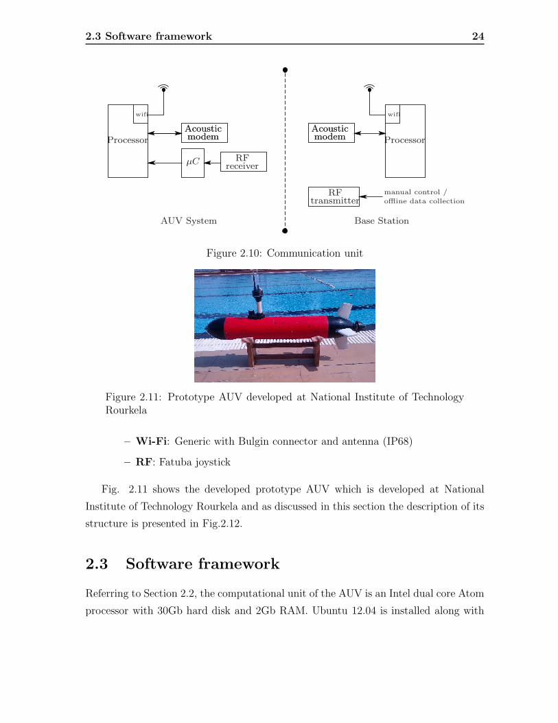
2.3 Software framework 24

ProcessorAcousticmodem

µC RFreceiver

wifi

AUV System

Processor

wifi

Acousticmodem

AcousticmodemAcousticmodem

Base Station

transmitterRF manual control /

offline data collection

Figure 2.10: Communication unit

Figure 2.11: Prototype AUV developed at National Institute of TechnologyRourkela

– Wi-Fi: Generic with Bulgin connector and antenna (IP68)

– RF: Fatuba joystick

Fig. 2.11 shows the developed prototype AUV which is developed at National

Institute of Technology Rourkela and as discussed in this section the description of its

structure is presented in Fig.2.12.

2.3 Software framework

Referring to Section 2.2, the computational unit of the AUV is an Intel dual core Atom

processor with 30Gb hard disk and 2Gb RAM. Ubuntu 12.04 is installed along with


1

2

3

4

5

68

9

11

12

13

14

11

7 6

1

12

5

12

4

6 7

8

10

5

13

3

1

2

3

4

Nose Section

Hull Section

Tail Section

Top rudder plane

6

7

8

Starboard stern plane

Portside stern plane

Kort Nozzle9

10

11

12

Thruster

Propeller

Acoustic modem

GPS. Wifi, RF

13

14

DVL

Access to internal units

5 Bottom rudder plane

Figure 2.12: Different parts of the developed AUV


the following software packages for the execution of the AUV algorithms

• Robot Operating System (ROS) [55]: It is originated at Stanford Artificial In-

telligence Lab and further developed and maintained by Willow Garage. ROS

packages are used to integrate various sensor, actuator units and computational

units. It is a set of libraries and tools which are used to write driver programs

for sensors and control algorithms. Some of the terminologies used in ROS as

follows

– Nodes: Nodes are processes that perform computation. ROS is designed

to be modular, it may consist of multiple nodes. For example, one node

controls a laser range-finder, one node controls the wheel motors, one node

performs localization, one node performs path planning, one Node provides

a graphical view of the system, and so on.

– Topics: A node sends out a message by publishing it to a given topic. The

topic is a name that is used to identify the content of the message. It may

be the information regarding velocity, speed, temperature etc.

– Messages: Nodes communicate with each other by passing messages. A

message is simply a data structure comprising typed fields.

In ROS intermediate nodes are created to acquire, process and transmit the

data as shown in Fig.2.13. The sensor messages and actuator messages are

the information required or generated from the computational unit. ROS is

implemented in the developed AUV and each sensor and actuators are interfaced.

• MOSEK: MOSEK ApS provides free academic license to solve various convex

optimization problem. For the developed AUV, it is used to solve constrained

quadratic programming problem discussed in Chapter 4 and a constrained robust

optimal control problem discussed in chapter 5 respectively.

2.4 Chapter Summary 27

Figure 2.13: Example of ROS structure considering Computer, Sensor andActuator as the Nodes

2.4 Chapter Summary

In this chapter, design and development of a prototype Autonomous Underwater Ve-

hicle in the laboratory are presented. It discusses about the design specification of

the nose and tail profile of the AUV. Further, the hardware configuration required

to achieve autonomous capability is also discussed. The software framework which is

required for interfacing of various sensors and also for the controller implementation

is presented.

Chapter 3

LoS Guidance Law using Inverse

Optimal Self-Tuning Adaptive

Controller

In chapter 2, design and development of the prototype AUV is discussed. The de-

veloped AUV will be used for the experimental verification of the control algorithms.

As stated in chapter 1, among various motion control schemes, path following and

way-point tracking are suitable for underactuated AUVs. These algorithms can be

implemented using LoS based guidance algorithms as presented in [19]. Further, an

adaptive control strategy should be adopted to address the issue of payload variation

or for resolving unknown AUV dynamics. Therefore, this chapter focusses on the de-

velopment of a LoS based guidance control algorithm using Nonlinear Autoregressive

Moving Average eXogenous (NARMAX) identified AUV dynamics for both heading

as well as diving motion. Among various NARMAX structures as discussed in [1],

polynomial-based NARMAX model structure is chosen because of its simplicity in

control design. The parameters of the NARMAX model structure are updated on-line

using Recursive Extended Least Square (RELS) algorithm in order to capture the un-

known AUV dynamics. Using these parameters, an adaptive PID controller is designed

for the implementation of the LoS guidance algorithm. The gain parameters of the

PID controller are then tuned on-line at every kth instant using an inverse optimal

control technique [57], which alleviates the problem of solving a Hamilton-Jacobian

3.1 Problem Statement 29

equation for generating a suitable control signal.

The chapter is organized as follows. Section 3.1 presents the problem statement ad-

dressed in this chapter. Further, the development of nonlinear identification technique

for capturing AUV dynamics is described in Section 3.2. The obtained parameters are

then used to develop an adaptive controller for both AUV kinematics and dynamics.

The proposed control algorithm has been derived in two steps i.e. kinematic controller

in Section 3.3.1 and dynamic controller in Section 3.3.2. The implementation of the

control algorithm in a prototype AUV is discussed in Section 3.5, which envisages the

effectiveness of the identification algorithm and LoS guidance algorithm. The chapter

is concluded in Section 3.6.

3.1 Problem Statement

In order to develop a guidance algorithm for an torpedo shaped underactuated AUV,

the roll motion is assumed to be zero and a constant surge velocity is considered

throughout this work. Thus, considering these assumptions the kinematics and dy-

namics equation for an AUV is given as follows,

η = J (η) ν, (3.1a)

Mν + Cr (ν) ν + fd (ν) + rs (η) = τ. (3.1b)

In the kinematic expression (3.1a), the variable η = [x, y, z, θ, ψ]T ∈ R5 denotes posi-

tion vector in earth-fixed frame I and ν = [v, w, q, r]T ∈ R4 is the velocity vector

in the body-fixed frame B. J(η) ∈ R5×4 is the transformation matrix from B to

I.

Separate AUV dynamics (3.1b) can be considered for heading motion [v, r]T and

diving motion [w, q]T for the simplification of the control design. However the physical

parameters of the AUV dynamics get affected when payload or/and physical structure

is modified. Therefore, as discussed in chapter 1, a NARMAX identification technique

is to be adopted for the identification of the AUV dynamics as shown in Fig.3.1.

Further, a cascade control strategy is adopted for designing separate controllers for

kinematics and dynamics. Using the path error, the controller for kinematics should


AUV Kinematics

NARMAX Heading

KinematicsController

Way-Point

X

YLoS Path

Desired LoS Path

AUV Dynamics

v

w

q

r

[

δrδs

]

x

y

z

θ

ψ

NARMAX Diving

DynamicsController

AdaptationMechanism

NARMAX Identification

[

rdqd

]

Figure 3.1: Structure of the proposed NARMAX model based self-tuningcontroller

generate desired velocities [rd qd]T for the AUV dynamics. These velocities are to be

followed by an AUV in order to track a desired path. Therefore, another controller

for AUV dynamics should be designed which generates suitable actuation signal i.e.

[δr δs]T as shown in Fig.3.1. However, few assumptions are considered throughout

this work i.e.

Assumption 3.1. All the states of the kinematic equation (3.1a) and dynamic equa-

tion (3.1b) are measurable.

Remark 3.1. Considering the physical constraint or cost of the sensor system, the

Assumption 3.1 is not always true. However, an observer can be designed as in [58],

to estimate the unmeasured states of the AUV.

Assumption 3.2. The effect of rudder and stern plane on sway and heave motion is

zero i.e. Yuuδr = Zuuδs = 0.

Remark 3.2. For an underactuated AUV, the inclusion of these terms complicates

the controller design with no significant improvement in the tracking performance [17].

Unlike a fully-actuated vehicle, the effect of rudder and elevator fins along sway and

heave motion is less significant, thus it can be neglected for the design of control law.

Assumption 3.3. Throughout this work, the surge velocity uc of the AUV is assumed

to be constant.

3.2 Identification of the AUV dynamics 31

Remark 3.3. Considering an underactuated AUV, this assumption is generally adopted

for path following problem because the desired path is independent of the time con-

straint. Further, an independent controller for surge motion can be designed to main-

tain a desired velocity.

Assumption 3.4. Roll angle and roll rate are assumed to be zero.

Remark 3.4. Although during some maneuvers, the roll oscillations may be signif-

icant. However, most of the AUVs maintain a vertical distance between center of

gravity (CG) and center of buoyancy (CB) so as to decay the roll oscillation. Fur-

ther, a decoupling method [59] or a separate roll-stabilization mechanism [60] can be

employed to compensate the roll oscillations.

Assumption 3.5. It is assumed to have two separate identification schemes for head-

ing and diving motions.

Limitation 1. In certain maneuvers the interaction of roll motion with the heading

and diving dynamics is significant in nature, so during this instant Assumption 3.5

will not be effective.

Remark 3.5. Assumption 3.5 is desirable as it simplifies the controller design; the

inherent characteristics of the controller to follow a desired path will eventually com-

pensate the error accumulated due to Limitation 1.

3.2 Identification of the AUV dynamics

System identification technique is suitable for capturing the AUV dynamics in real-

time. Among the various system identification techniques, NARX model is a suitable

paradigm for real-time implementation as mentioned in [61]. In spite of NARX model,

a NARMAX model introduced in [1] can also be utilized for capturing the system

dynamics more accurately. The general structure of the NARMAX model is given as

yp (k) = f (yp (k − 1) , . . . , yp (k −m) , up (k − 1) , . . . , up (k − n)) , (3.2)

where f (·) represents a nonlinear function consisting of delayed system output and

control input, yp(·) is the system output and yp(·) is the estimated output from the


System∑

z−1

z−1

z−1 z−1

z−1

z−1

f(·)

up(k)

yp(k) ep(k)

yp(k)

+

−

Figure 3.2: NARMAX model structure for system identification [1]

NARMAX structure. The general structure for the implementation of the NARMAX

model in order to identify any dynamical system is shown in Fig.3.2. Referring to

Fig.3.2, the output error of the NARMAX structure is used to tune the model param-

eters at every time instant.

In this work, polynomial based NARMAX model is used to identify the AUV

dynamics which constituents of heading and diving motion. Heading motion includes

sway and yaw motion [vk rk]T whereas the diving motion includes heave and pitch

motion i.e. [wk qk]T . Two separate NARMAX structures are used to identify the

heading and diving motion and for updatation of its parameter RELS algorithm is

employed. Referring to [62], the NARMAX model for the heading motion is given by

[

vk

rk

]

=

[

f11(vk−1, rk−1)

f21(vk−1, rk−1)

]

+

[

g11

g21

]

δr,k−1 +

[

d11

d21

]

e1,k−1, (3.3)

where

f11(vk−1, rk−1) = α01vk−1 + α11rk−1 + α21v2k−1 + α31r

2k−1 + α41vk−1rk−1,


g11 = α51,

f21(vk−1, rk−1) = β01vk−1 + β11rk−1 + β21v2k−1 + β31r

2k−1 + β41vk−1rk−1,

g21 = β51,

Similarly, the NARMAX model for diving motion is given by

[

wk

qk

]

=

[

f12(wk−1, qk−1)

f22(wk−1, qk−1)

]

+

[

g12

g22

]

δs,k−1 +

[

d12

d22

]

e2,k−1, (3.4)

where

f12(wk−1, qk−1) = α02wk−1 + α12qk−1 + α22w2k−1 + α32q

2k−1 + a42wk−1qk−1,

g12 = α52

f22(wk−1, qk−1) = β02wk−1 + β12qk−1 + β22w2k−1 + β32q

2k−1 + β42wk−1qk−1,

g22 = β52,

In case of a torpedo shaped AUV with rear thruster for forward motion and control

planes for orientation, there is no actuation along the sway and heave motion. There-

fore, g11 and g12 in (3.3) and (3.4) can be termed as zero. These equations (3.3) and

(3.4) can be represented as

Yi,k = φTi,k−1δi,k−1, (3.5)

for i = 1, 2. Referring to (3.5), φi,k−1 and δi,k−1 represents the regressor and param-

eter vector respectively. For i = 1, Y1,k = [vk rk]T is considered for the identification

of the heading dynamics. Similarly, Y2,k = [wk qk]T is used to identify the diving

dynamics of the AUV. A Recursive Extended Least Square (RELS) algorithm [63]

is employed due to unmeasurable noise terms [e1,k e2,k]T . The expression for RELS

algorithm for determining the estimated parameters are as follows,

δi,k = δi,k−1 +Si,k−1φi,k−1

λk−1 + φTi,k−1Si,k−1φi,k−1εi,k−1,

Si,k =1

λk−1

Si,k−1 −Si,k−1φi,k−1φ

Ti,k−1Si,k−1

λk−1 + φTi,k−1Si,k−1φi,k−1

,

Yi,k = φTi,k−1δi,k−1 + εi,k−1,

3.3 Development of the Adaptive Inverse-Optimal PID Controller 34

δh

Uk

uk

vk

βhψk

xk

yk

B

dk=0

dk > 0

dk < 0

LOS-path

ith waypoint

(i− 1)th waypoint

Figure 3.3: Desired LoS path

λk = λ0λk−1 + (1− λ0), (3.6)

where λk, Si,k and εi,k−1 are the forgetting factor, covariance matrix and residual error

output. In the subsequent section, a motion control scheme is developed using the

identified model of the AUV.

3.3 Development of the Adaptive Inverse-Optimal

PID Controller

The objective of path following control is achieved through designing separate con-

trollers for kinematics and dynamics of the AUV. For kinematics, a Lyapunov based

backstepping control is designed in section 3.3.1 to minimize the position and orienta-

tion error respectively. Further, a self-tuning PID controller is designed in section 3.3.2

for the AUV dynamics. This control law generates actuation signals for rudder and

stern plane in order to steer the AUV along the LoS path. The detailed description of

these controller development is presented in the subsequent sections.


3.3.1 Control design for kinematics

Referring to Fig. 3.3, let a LoS path with constant depth reference is to be followed

by an AUV. From the figure, the expression for cross-track error can be deduced as

dk = 〈A,Xk −X0〉 − C (3.7)

where

A =

[

a11 a12 0

a21 0 a23

]

, Xk −X0 =

xk − x0

yk − y0

zk − z0

, C =

[

c1

c2

]

.

where A represents the path parameters and X0, C represents the offset from the

desired path. Further, the dk = [ye,k ze,k]T is defined as the cross-track error along the

heading and diving motion respectively. In the subsequent section, the control input

for AUV kinematics i.e. desired pitch and yaw velocities are derived for minimizing

these cross-track errors to zero.

Diving Control

Referring to [64], the kinematic equations for the diving motion is expressed as follows

zk = zk−1 + Ts (−uc sin θk−1 + wk−1 cos θk−1) , (3.8a)

θk = θk−1 + Tsqk−1. (3.8b)

Let the AUV is required to track a desired depth reference zd, then the modified diving

cross-track error for non-zero reference is given by

ze,k = zk − zd. (3.9)

ze,k should be minimized at every kth instant. Therefore, a Lyapunov candidate func-

tion can be chosen as

V1,k =1

2ze,k

2 (3.10)


and by showing that V1,k − V1,k−1 ≤ 0, the cross-track error ze,k will always reduce to

zero. Substituting zk from (3.8a) into (3.10), the objective function V1,k can be written

as

V1,k = V1,k−1 + TsUcwze,k−1sin(θk−1 − δd) +1

2T 2s sin

2(θk−1 − δd), (3.11)

where δd = tan−1(wk−1/uc) is the angle of attack and Ucw =√

(u2c + w2k−1) is the

resultant velocity in the vertical axis. Assuming that sampling time Ts << 1, the

equation (3.11) is expressed as

V1,k − V1,k−1 = TsUcwze,ksin(θk−1 − δd). (3.12)

In order to minimize the Lyapunov function V1,k at each sampling instant, it is neces-

sary that the following condition should be satisfied i.e.

V1,k − V1,k−1 ≤ 0. (3.13)

Therefore, referring to (3.12), the condition (3.13) will be satisfied if

TsUcwze,ksin(θk−1 − δd) ≤ 0. (3.14)

Since Ts and Ucw are always positive, therefore a desired pitch angle can be chosen as

θk−1 = −θae2Kδze,k−1 − 1

e2Kδze,k−1 + 1+ δd, (3.15)

where θa is the maximum approaching angle and Kδ is a positive term respectively.

For kth instant, equation (3.15) represents the desired pitch orientation (θd,k) and it is

required to minimize the difference between the actual and desired pitch orientation.

Therefore, an error in pitch orientation (eθ,k) is defined as follows

eθ,k = θk − θd,k. (3.16)

In order to minimize the pitch orientation error, eθ,k must satisfy the following condi-

tion i.e.

eθ,k = ξ1eθ,k−1 (3.17)


where ξ1 ∈ (0, 1). By substituting θk from (3.8b) in (3.17), the desired pitch velocity

for kth instant is given by

qd,k =1

Ts(ξ1θk−1 − ξ1θd,k−1 + θd,k − θk−1) , (3.18)

The desired pitch velocity qd,k will be further used in Section 3.3.2 to derive a suitable

actuation signal for AUV dynamics.

Heading Control

Referring to [64], the heading motion is governed by the following kinematic equations

i.e.

xk = xk−1 + Ts

(

u′

k−1 cosψk−1 − vk−1 sinψk−1

)

, (3.19a)

yk = yk−1 + Ts

(

u′

k−1 sinψk−1 + vk−1 cosψk−1

)

, (3.19b)

ψk = ψk−1 + Ts sec θk−1rk−1, (3.19c)

where u′

k−1 = (uc cos θk−1 + wk−1 sin θk−1) is the projection of the net velocity along

the surge motion of B and as specified earlier Ts is the sampling time. Using these

kinematic equations, the desired yaw velocity should be derived such that the cross-

track error along the heading motion should be minimized. Thus, referring to (3.7)

the cross-track error is expressed as

ye,k = a11xk + a12yk. (3.20)

By substituting xk and yk from (3.19) into (3.20), the modified expression for cross-

track error is given as

ye,k = ye,k−1 + TsUk (a11 cos (ψk−1 + β) + a12 sin (ψk−1 + β)) , (3.21)

where βk = tan−1(

vkuc

)

is the side-slip angle and Uk =√

u′

k−12+ v2k−1 is the resultant

velocity. Further, the expression (3.21) can be reduced to

ye,k = ye,k−1 + TsUka sin (ψk−1 + βk − δh) , (3.22)


where δh = tan−1 −a11a12

denotes the slope of the LoS path and a =√

a211 + a212 is the

resultant value. In order to minimize the cross-track error ye,k, a Lyapunov candidate

function V2,k ≥ 0 is chosen as

V2,k =1

2y2e,k (3.23)

Assuming that Ts << 1, the candidate function V2,k can be expressed as

V2,k = V2,k−1 + TsUkaye,k−1 sin (ψk−1 + βk − δh) . (3.24)

Thus, to minimize V2,k at every kth instant, the following condition should always be

satisfied i.e.

Ukaye,k−1 sin (ψd,k) ≤ 0, (3.25)

where ψd,k is the desired yaw orientation. In (3.25), Uk and a are always positive

therefore ψd,k can be chosen as

ψd,k = −θae2Kδyek−1 − 1

e2Kδyek−1 + 1. (3.26)

Referring to Fig.3.3, considering the desired approaching angle ψd,k from (3.26), the

orientation error between B and F is given by

ψe,k = ψk + βk − δh − ψd,k, (3.27)

where δh is the slope of the desired path and (ψk + βk) is the orientation of the resultant

velocity Uk w.r.t. I. Using (3.27) and substituting ψk from (3.19c), the desired yaw

rate at kth instant is

rd,k =cos θk−1

Ts(ξ2ψe,k + ψd,k + δh − βk − ψk−1) , (3.28)

where ξ2 ∈ (0, 1). The desired velocities (3.18) and (3.28) are obtained using the AUV

kinematic equations. In section 3.3.2, a suitable actuation signal is generated so that

the actual velocities track the desired velocities. Thus, it enables the AUV to track

the desired path.


3.3.2 Control design for dynamics

In this section, the suitable actuation signals for AUV dynamics have to be obtained

such that the actual velocities qk and rk should track the desired velocities qd,k and

rd,k. As discussed in section 3.3.1, the NARMAX model structure for heading motion

and diving motion can be represented as

νk = f(νk−1) + g(νk−1)µk−1, (3.29)

where νk ∈ R2 and µk ∈ R are the states and input of the system.

Theorem 3.1. [65] For an affine nonlinear function (3.29), let an output is defined

as

yk = h(νk−1, νδ,k) + J(νk−1)µk−1. (3.30)

Considering a Lyapunov function Vk−1 = 12νTe,k−1P νe,k−1, where νe,k−1 = νk − νδ,k is

the difference between the actual and desired state. The passivity condition

Vk − Vk−1 ≤ yTk−1µk−1, (3.31)

is always satisfied if,

µk−1 = −(Im + J(νk−1))−1h(νk−1, νδ,k), (3.32)

where

h(νk−1, νδ,k) = gT (νk−1)P (f(νk−1)− νδ,k),

J(νk−1) =1

2gT (νk−1)P g(νk−1). (3.33)

The control input expressed in (3.32) can also be expressed in terms of ek as follows

µk−1 = −(Im − J(νk−1))−1gT (νk−1)P ek. (3.34)

By substituting (3.29) into (3.34), the control law becomes complex and it is not feasi-

ble for implementation as the control input µk−1 depends on future instant. Therefore,


a local linear model is identified in order to simplify the control structure. In view

of feasibility of the controller, an adaptive self-tuned PID controller is adopted. Us-

ing [62], a linearized expression for (3.29) is presented as

νk = Ak−1νk−1 +Bk−1µk−1 + Lk−1ek−1,lin, (3.35)

where ek,lin = νk − νδ,k and Lk−1 is the observer gain. Considering the observer gain

Lk−1 as

Lk−1 =[

(Pk−1 +R)−1Pk−1ATk−1

]T, (3.36)

ensures that the eigen values of the linearized model (3.35) always lie within the unit

circle. In (3.36), R defines the covariance of the noise. Pk−1 is the solution of the

Riccati equation given in (3.37).

Ak−1Pk−1ATk−1 − Pk−1 − (Ak−1Pk−1) (Pk−1 +Rk−1)

−1 (Pk−1ATk−1

)

+Qk−1 = 0. (3.37)

By replacing ek with ek,lin in (3.34), the control law can be written as

µk−1 = −(Im − J(νk−1))−1gT (νk−1)P ek,lin, (3.38)

where ek,lin = νk − νδ,k and P > 0 is a weight variable. Substituting (3.35) into (3.38)

yields

µk−1 =(

Im − J (νk−1) + gT (νk−1)B)−1 [

−gT (νk−1)P(A+ Lk−1)ek−1,lin + Aνδ,k−1 − νδ,k]

.

(3.39)

The derived control law satisfies the requirements for the stability of the closed loop

system. The control law is adaptive to the payload variation or modification to the

physical structure due to the NARMAX identification of the AUV dynamics. Further,

(3.39) is realized as an adaptive PID controller where the gains of the PID controller

are updated at each instant in order to steer the AUV along the desired path. Let

P = 1 + P12z−1 + P13z

−2, then (3.39) can also be represented as

µk−1 = X1 +X2z−1 +X3z

−2, (3.40)

3.4 Stability Analysis 41

where

X1 = −(

Im − J(νk−1) + gT (νk−1)B)−1

gT (νk−1)(A + Lk−1)ek−1,

X2 = −(

Im − J(νk−1) + gT (νk−1)B)−1

gT (νk−1)P12(A+ Lk−1)ek−2,

X3 = −(

Im − J(νk−1) + gT (νk−1)B)−1

gT (νk−1)P13(A+ Lk−1)ek−3.

Referring to [66], the discrete-time PID control law is expressed as

µk−1 =

(

kci

(

1 +TsTIi

+TDiTs

)

− kci

(

1 +2TDiTs

)

z−1 + kciTDiTs

z−2

)

ek−1, (3.41)

and by comparing (3.41) with (3.40), the gains of the PID controller can be obtained

as follows

kci = −(X2 + 2X3), (3.42)

TDi = −X3

(X2 + 2X3)Ts, (3.43)

TIi = −X2 + 2X3

(X1 +X2 +X3)Ts. (3.44)

However, the control law (3.39) and the adaptive PID controller (3.41) are equivalent

but (3.41) is more suitable in view of implementation.

In view of controller design for heading motion the variables of (3.29) becomes

νk = [vk rk]T and µk = δr,k, whereas for diving motion νk = [wk qk]

T and µk = δs,k

respectively.

3.4 Stability Analysis

Let a Discrete-Time Control-Lyapunov Function (DTCLF) for tracking the desired

state xδ,k,

V (νk, νδ,k) =1

2(νk − νδ,k)

T P (νk − νδ,k) (3.45)

If the derived control input satisfies the passivity condition i.e.

V (νk, νδ,k)− V (νk−1, νδ,k−1) ≤ σk−1Tµk−1 (3.46)

3.4 Stability Analysis 42

then the system (3.29) is said to be globally asymptotic stable. Referring to [65], σk−1

can be written as

σk−1 = h(νk−1, νδ,k) + J(νk−1)µk−1. (3.47)

Thus, rewriting the passivity condition (3.46) by replacing σk−1 from (3.47) is given

by

V (νk, νδ,k)− V (νk−1, νδ,k−1) ≤ h (νk−1, νδ,k)T µk−1 + µTk−1J (νk−1)µk−1 (3.48)

where h(νk−1, νδ,k) is given by

h(νk−1, νδ,k) = gT (νk−1)P (ek+1 − g(νk−1)µk−1) (3.49)

the passivity condition of (3.46) becomes

V (νk, νδ,k)− V (νk−1, νδ,k−1) ≤ ekT P g(νk−1)µk−1 − µk−1

T(

g(νk−1)T P g(νk−1)− J (νk−1)

)

µk−1

≤ ek+1,linT P g(νk−1)µk−1 − µk−1

Tg(νk−1)T P g(νk−1)µk−1 +

µTk−1J (νk−1)µk−1 + eTk+1P g(νk−1)µk−1 (3.50)

ek+1 is the difference between actual error ek+1 and approximated error ek+1,lin derived

from the linearized model. Using (3.38), equation (3.50) is expressed as,

V (νk, νδ,k)− V (νk−1, νδ,k−1) ≤ µk−1T (−Im + J (νk−1))µk−1 − µk−1

Tg(νk−1)T P g(νk−1)µk−1 +

µTk−1J (νk−1)µk−1 + eTk+1P g(νk−1)µk−1

≤ −µk−1T(

−Im + J (νk−1)− g(νk−1)T P g(νk−1)+

J(νk−1))µk−1 + eTk+1P g(νk−1)µk−1 (3.51)

∥

∥eTk+1P g(νk−1)µk−1

∥

∥ < ρ, where ρ is a positive constant. The term eTk+1P g(νk−1)µk−1

is always bounded because an observer gain is designed in (3.36) which reduces the

ek+1 error. Thus, equation (3.51) can be expressed as

V (νk, νδ,k)− V (νk−1, νδ,k−1) ≤ −µk−1Tµk−1 + ρ, (3.52)

which satisfies the passivity condition.

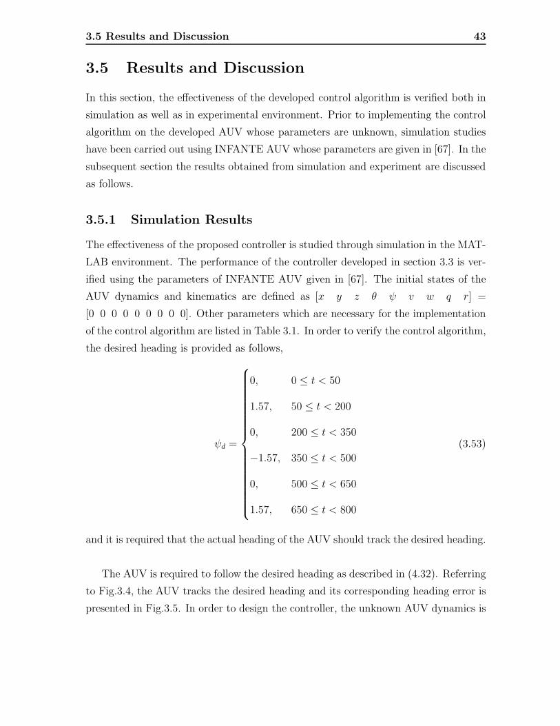
3.5 Results and Discussion 43

3.5 Results and Discussion

In this section, the effectiveness of the developed control algorithm is verified both in

simulation as well as in experimental environment. Prior to implementing the control

algorithm on the developed AUV whose parameters are unknown, simulation studies

have been carried out using INFANTE AUV whose parameters are given in [67]. In the

subsequent section the results obtained from simulation and experiment are discussed

as follows.

3.5.1 Simulation Results

The effectiveness of the proposed controller is studied through simulation in the MAT-

LAB environment. The performance of the controller developed in section 3.3 is ver-

ified using the parameters of INFANTE AUV given in [67]. The initial states of the

AUV dynamics and kinematics are defined as [x y z θ ψ v w q r] =

[0 0 0 0 0 0 0 0 0]. Other parameters which are necessary for the implementation

of the control algorithm are listed in Table 3.1. In order to verify the control algorithm,

the desired heading is provided as follows,

ψd =

0, 0 ≤ t < 50

1.57, 50 ≤ t < 200

0, 200 ≤ t < 350

−1.57, 350 ≤ t < 500

0, 500 ≤ t < 650

1.57, 650 ≤ t < 800

(3.53)

and it is required that the actual heading of the AUV should track the desired heading.

The AUV is required to follow the desired heading as described in (4.32). Referring

to Fig.3.4, the AUV tracks the desired heading and its corresponding heading error is

presented in Fig.3.5. In order to design the controller, the unknown AUV dynamics is


Table 3.1: Simulation parameters

Ts = 0.5 θa = 0.52 Kδ = 0.4 uc = 0.8ξ1 = 0.8 ξ2 = 0.8

0 100 200 300 400 500 600 700 800−2

−1.5

−1

−0.5

0

0.5

1

1.5

2

Time (sec)

Headingangle

(ψ)

(inrad)

Actual headingDesired heading

Figure 3.4: Tracking of desired heading by INFANTE AUV

identified using polynomial based NARMAX structure at every time instant. Fig.3.6

compares the identified yaw motion with the actual yaw motion and from the figure

it is evident the polynomial-based NARMAX structure is suitable. Further, the

updatations of its parameters are given in Fig.3.7. Using these parameters the control

law (3.41) is implemented and the generated actuation signal i.e. δr to steer the AUV

along the yaw motion is shown in Fig.3.8. In this work, it is assumed that the control

planes varying from −0.785 rad to 0.785 rad, therefore the actuation signal exceeding

0 100 200 300 400 500 600 700 800

−1.5

−1

−0.5

0

0.5

1

1.5

Time (sec)

Headingerror

(inrad)

Figure 3.5: Heading error


0 100 200 300 400 500 600 700 800−0.15

−0.1

−0.05

0

0.05

0.1

0.15

0.2

Time (sec)

Yaw

velocity

(rad/sec)

Actual velocityEstimated velocityLinearized velocity

217 218 2190.06

0.065

0.07

Figure 3.6: Estimated yaw velocity as compared to actual yaw velocity

0 100 200 300 400 500 600 700 800−0.5

0

0.5

1

1.5

2

Time (sec)

Parametersupdatation

β0β1β2β3β4

Figure 3.7: Updatation of the NARMAX parameters for yaw motion

0 100 200 300 400 500 600 700 800−0.8

−0.6

−0.4

−0.2

0

0.2

0.4

0.6

0.8

Time (sec)

Rudder

orientation(δ

r)

(inrad)

Figure 3.8: Actuation signal while tracking a desired heading


Table 3.2: Description of ROS nodes

Node Description/xsens driver Driver node to access Xsens MTI INS sensor/navquest node Driver node to access Navquest DVL sensor/odom trans Generates AUV states/controller self tuning PID Controller node (3.41)/narmax NARMAX node for identification (3.2)/narmax linearized Linearized AUV velocities (3.35)/rosserial server Arduino node for transmitting actuation signal

these extremum values is clipped using a limiter. From the obtained results, it is

evident that the NARMAX model structure along with the self-tuning PID control

algorithm is effective for controlling AUV motion.

3.5.2 Experimental Results

From the simulation results, it is confirmed that the system identification technique

and the developed control algorithm is suitable for controlling the AUV. Further, in this

section the control algorithm is verified in the prototype AUV. As discussed in chapter

1, the prototype AUV is installed with Ubuntu 12.04 and ROS Hydro [55]. Therefore,

ROS nodes of the identification and control algorithm as shown in Fig.3.9 is designed

which accepts the data from the AUV sensor nodes and generate the actuation signal

to the AUV actuation nodes. The description of these nodes is presented in Table 3.2

and the characteristics of their messages such as bandwidth, frequency etc are shown

in Table 3.3.

Figure 3.9: Communication between ROS nodes

The experimentation is conducted at National Institute of Technology Rourkela

swimming pool having length 10m, breadth 5m and maximum depth 1.6m. Let, the


Table 3.3: Description of ROS messages and its characteristics

Message Description Bandwidth Publishing rate/imu data φ, θ, ψ, p, q, r 32.8 Kb/sec 100/auv states z, φ, θ, ψ, u, v, w, p, q, r 523 B/sec 10/linearized vel v, w, q, r 525 B/sec 10/estvel v, w, q, r 522 B/sec 10/rudder ang δr 20 B/sec 10/altitude z 20 B/sec 10

Table 3.4: Parameters

Ts = 0.1 θa = 0.52 Kδ = 0.1 uc = 1ξ1 = 0.1 ξ2 = 0.8

desired heading reference similar to (4.32) is considered as follows

ψd =

0, 0 ≤ t < 5

1.57, 5 ≤ t < 20

0, 20 ≤ t < 35

−1.57, 35 ≤ t < 50

0, 50 ≤ t < 65

1.57, 65 ≤ t < 75

(3.54)

and the initial states of the AUV is [x, y, z, θ, ψ, v, w, q, r]T = [0, 0, 0, 0, 0, 0, 0, 0, 0]T .

The implementation of the control algorithm in the prototype AUV is shown in

Fig.3.10. Throughout the experimentation the surge velocity of the AUV is assumed

to be constant i.e. 0.8 m/sec. Further, the design parameters considered during the

experimental verification of the control algorithm is presented in Table 3.4.

Referring to Fig.3.11, the prototype AUV tracks the desired heading orientation

(4.32) and the corresponding heading error is presented in Fig.3.12. Referring to

Fig.3.14, the designed polynomial-based NARMAX structure is used to identify the

AUV dynamics at each sampling time and the obtained parameters as shown in


DVL[u v]

GPS[x y]

Depth Sensorz

INS[ǫ2 ǫ3 η p q r]

NARMAX Heading

DynamicsController


PWM

Generation

Thruster

Stern

SensorFusion

[vk rk] δr,k

T

δs,pwm

Sensor Unit Computational Unit Actuation Unit

ROS

Linux OS

Rudderδr,pwm

δs,k[wk qk]NARMAX Diving

Figure 3.10: Implementation of the self-tuning controller

0 10 20 30 40 50 60 70−2

−1.5

−1

−0.5

0

0.5

1

1.5

2

Time (sec)

Yaw

orientation(ψ

)(inrad)

Desired yaw angleActual yaw angle

Figure 3.11: Tracking of desired heading

Fig.3.15 are then used to develop a control algorithm. Using these parameters the

control law defined in (3.41) generates the actuation signal as shown in Fig.3.17 and

the controller parameters are shown in Fig.3.16. Similar to the simulation studies, the

control planes varies between −0.785 rad to 0.785 rad, therefore the actuation signal

exceeding these extremum values is clipped using a limiter. The computational time

taken by the algorithm is shown in Fig. 3.18 and it is found that the maximum time

taken by the algorithm to generate an actuation signal is 0.011 sec. From the obtained

results, it is clear that the control algorithm is suitable for practical realization but

the issues of actuator saturation which results windup needs to be addressed.


0 10 20 30 40 50 60 70−1.5

−1

−0.5

0

0.5

1

1.5

Time (sec)

Headingerror

(inrad)


0 10 20 30 40 50 60 70−0.15

−0.1

−0.05

0

0.05

0.1

0.15

0.2

Time (sec)

Pitch

velocity

(rad/sec)

ActualEstimated

37 38 390.080.09

Figure 3.13: Pitch rate of the AUV during path follow

0 10 20 30 40 50 60 70−0.4

−0.3

−0.2

−0.1

0

0.1

0.2

0.3

0.4

0.5

Time (sec)

Yaw

velocity

(rad/sec)

ActualEstimated

25 26 27

0.10.120.14

Figure 3.14: Yaw rate of the AUV during path follow


0 10 20 30 40 50 60 70

−0.5

−0.4

−0.3

−0.2

−0.1

0

0.1

0.2

0.3

Time (sec)

Parameters

β0

β1

β2

β3

β4

Figure 3.15: Updatation of the NARMAX parameters

0 500 1000 1500 2000 2500 3000 3500 4000 4500−20

−15

−10

−5

0

5

Time

Controller

gains

TDi

TIi

kci

1800 2000 2200−0.144

−0.142

Figure 3.16: Updatation of the controller gain parameters

0 10 20 30 40 50 60 700

10

20

30

40

50

60

70

80

90

Time (sec)

Rudder

orientation(δ

r)

(inrad)

Figure 3.17: Rudder plane orientation while following a desired path


0 10 20 30 40 50 60 700

0.002

0.004

0.006

0.008

0.01

0.012

Time (sec)

Computationaltime(sec)

Figure 3.18: Computational time required to generate the actuation signal

3.6 Chapter Summary

In this chapter, a LoS guidance control algorithm is proposed which involves two steps.

Firstly, a kinematic controller is designed which provides the reference for the dynamic

controller. The kinematic controller is designed using backstepping controller and

stability is proved using the Lyapunov theory. For the design of dynamic controller,

first the dynamic model of the AUV is identified using NARMAX model and the

parameters of the AUV are updated using RELS method. An inverse optimal controller

is applied to design a Self-Tuning PID controller. This PID controller generates the

control signal for the AUV to achieve path following task.

Chapter 4

Constrained Self-Tuning Adaptive

Controller for an AUV with

MR-NARMAX structure

Parameters of the AUV dynamics may vary due to change in payload or physical

structure. In view of resolving this parameter variation and obtaining efficient head-

ing and diving motion control algorithm, in this chapter a constrained self-tuning

controller (CSTC) is developed. A Nonlinear Auto-Regressive Moving Average eX-

ogenous (NARMAX) model is designed using the significant regressors to identify the

AUV heading and diving dynamics respectively. The parameters of the NARMAX

model are updated using a Recursive Extended Least Square (RELS) algorithm at

each time instant. Further, using the identified model a CSTC law is designed to track

desired waypoints using Line of Sight (LoS) guidance law. The controller gains are up-

dated at each instant satisfying the actuator constraint and computational efficiency is

studied in view of achieving practical implementation of the developed algorithm. The

efficacy of the developed NARMAX based CSTC algorithm to track a given reference

is verified in simulation as well as in experimental environment. From the obtained

results, it is concluded that the developed control algorithm is effective for an AUV to

track desired references.

The rest of the chapter is organized as follows. The design of a MR-NARMAX

structure for identifying AUV dynamics and updatation of its parameters are presented


AUV Kinematics


ControlAdjustment

Controller

Way-Point

X

YLoS Path

Desired LoS Path

AUV Dynamics

v

w

q

r

[

δrδs

][

Kp1

Kp2

]

x

y

z

θ

ψ

Figure 4.1: Controller Structure for the LOS Guidance law

in Section 4.2. Further, a constraint self-tuning adaptive control (CSTC) law for the

realization of LoS guidance law is presented in Section 4.3. Both the algorithms are

verified in an experimental environment which is discussed in Section 4.4. The chapter

is concluded in Section 4.5.


Referring to [64], the velocities ν = [v1 v2]T ∈ R

4 are defined in body-fixed frame

B along surge, sway, heave, roll, pitch and yaw motions, whereas the position of the

AUV η = [η1 η2]T ∈ R

5 is defined w.r.t earth-fixed frame I. η1 ∈ R3 and η2 ∈ R

2

are the linear and angular position of the AUV in I. To observe the motion of the

AUV from I, a transformation between B and I is necessary. So using the

transformation matrix J ∈ R5×4 from [9], the expression for velocities in I is given

by

η = J (η) ν. (4.1)

Equation (4.1) represents the kinematic description of the AUV, where η is the velocity

in I. Referring to [9], the dynamics of an AUV is given by

Mν + Cr (ν) ν + fd (ν) + rs (η) = τ. (4.2)

As discussed in chapter 1, variation in the AUV structure or payload alters the AUV

dynamics. Thus, a controller which depends on AUV parameters will not be effective

as compared to an adaptive controller. Further, for practical implementation of this

control strategy the physical limitations such as actuator constraints and computa-

4.2 Identification of the AUV Dynamics 54

tional efficiency should be considered. Therefore, an adaptive gain control strategy

along with the constraints i.e. CSTC strategy as shown in Fig.4.1 is to be developed

using the parameters obtained from a minimal-representation of an identified AUV

dynamics.

4.2 Identification of the AUV Dynamics

A polynomial based NARMAX structure is designed in Chapter 3 for the identification

of the AUV dynamics. But, NARMAX structure with redundant regressor terms

affects the computational burden. Thus, a minimal representation of the polynomial-

based NARMAX model i.e. MR-NARMAX using Forward Regression Orthogonal

Least Square (FROLS) method is designed. Further, the parameters of the identified

model are updated using a Recursive Extended Least Square (RELS) algorithm.

Referring to Assumption 3.5, common representation of the NARMAX structure

for heading and diving motion is given by

νk = f (ν1,k−1, ν2,k−1, uk−1) + deek−1. (4.3)

where νk = [ν1,k ν2,k]T ∈ R

2 is the estimated states, f = [f1 f2]T : R2 → R

2 is the

non-linear polynomial function used to identify the dynamics. Let N is the number of

regressor terms exist in a NARMAX structure then for i ∈ 1, · · · , N, αi and βi are

its parameters which are to be updated at each sampling time. de = [de1 de2]T ∈ R

2

are the disturbance parameters and ek−1 is the noise input. Eq (4.3) can be written

as follows

ν1,k = f1 (ν1,k−1, ν2,k−1, uk−1) + de1ek−1 (4.4a)

ν2,k = f2 (ν1,k−1, ν2,k−1, uk−1) + de2ek−1 (4.4b)

where

f1 (·) = α0ν1,k−1 + α1ν2,k−1 + α2ν21,k−1 + α3ν

22,k−1

+α4ν1,k−1ν2,k−1 + α5uk−1,


f2 (·) = β0ν1,k−1 + β1ν2,k−1 + β2ν21,k−1 + β3ν

22,k−1

+β4ν1,k−1ν2,k−1 + β5uk−1.

Using FROLS algorithm [1] significant state regressor terms of (4.4a) and (4.4b) are

identified. Let K samples are obtained through experimentation, then the equation

(4.4a) and (4.4b) can be represented as

Vi = Piωi, for i ∈ 1, 2 (4.5)

where Vi = [νi,1, . . . , νi,K ]T is the output vector, ωi ∈ R

N is the parameter vector and

Pi = [p1, p2 , · · · , pN ] ∈ RK×N is the regressor matrix respectively.

Example 1. For i = 1,

ν1 = [ν1,1, ν1,2, · · · , ν1,K ]T , ω1 =

[

α0 · · · α4

]T

,

P1 =

ν1,0 ν2,0 ν21,0 ν22,0 ν1,0ν2,0

ν1,1 ν2,1 ν21,1 ν22,1 ν1,1ν2,1...

......

......

ν1,K−1 ν2,K−1 ν21,K−1 ν

22,K−1 ν1,K−1ν2,K−1

Similarly for i = 2, ν2, ω2 and P2 can be derived.

For a matrix Pi, an orthogonal matrix Li ∈ RK×N and an upper triangular matrix

Υi ∈ RN×N exist for which

Pi = LiΥi, (4.6)

is always satisfied. Li consists of orthogonal columns as (l1, l2, · · · , lN) and referring

to [1] each element of Υi is defined as

γj,m =< pm, lj >

< lr, lj >, (4.7)

for 1 ≤ j ≤ m−1 and m = 2, 3, · · · , N . Rewriting (4.5), by substituting Pi from (4.6)

as

νi = LiGi, (4.8)


where Gi = [g1, g2, · · · , gN ]T = ǫ−1LTi νi and ǫ = LTi Li. The estimated parameters

using FROLS is given by

ωi = Υi−1Gi. (4.9)

To avoid overstated NARMAX structure (4.4), Error Reduction Ratio (ERR) can be

used to identify the significant regressor terms. ERR is defined as

ERRi = g2i< li, li >

νi, νi. (4.10)

The regressor terms with significant ERR value are considered to design the mini-

mal representation of (4.4) i.e. MR-NARMAX. The modified NARMAX structure is

represented as[

ν1,k

ν2,k

]

=

[

f1(ν1,k−1, ν2,k−1, uk−1)

f2(ν1,k−1, ν2,k−1, uk−1)

]

+

[

de1

de2

]

ek−1, (4.11)

where f1 and f2 consist of significant model terms.

Remark 4.1. For heading motion [ν1,k ν2,k]T = [vk rk]

T is considered, whereas for

diving motion [ν1,k ν2,k]T = [wk qk]

T respectively. Since, ν1,k is the velocity along sway

or heave motion, so for an underactuated AUV α5 = 0.

For s number of significant regressors, (4.11) can be modelled as

νi,k = φTi,k−1ωi,k−1, for i ∈ 1, 2, (4.12)

where φi,k−1 ∈ Rs and ωi,k−1 ∈ R

s are the significant regressor vector and estimated

parameter vector respectively. Then, a Recursive Extended Least Square (RELS)

method is employed for parameter estimation as

ˆωi,k = ˆωi,k−1 +Si,k−1φi,k−1

λk + φTi,k−1Si,k−1φi,k−1

εi,k−1,

Si,k =1

λk−1

Si,k−1 −Si,k−1φi,k−1φ

Ti,k−1Si,k−1

λk−1 + φTi,k−1Si,k−1φi,k−1

,

νi,k = φTi,k−1ˆωi,k−1 + εi,k. (4.13)

where λk, Si,k and εi,k−1 are the forgetting factor, covariance matrix and residual error

4.3 NARMAX Self-Tuning Controller Design 57

δh

Uk

uk

vk

βh,kψk

xk

yk

B

dk=0

dk > 0

dk < 0

LOS-path

ith waypoint

(i− 1)th waypoint

Figure 4.2: Tracking of Line of Sight path

output. The parameters obtained from (4.13) are used for developing an adaptive

controller to achieve waypoint tracking for an AUV as discussed in the subsequent

sections.

4.3 NARMAX Self-Tuning Controller Design

This section develops a control scheme for LoS guidance law by considering the iden-

tified AUV dynamics from Section 4.2. The line of sight guidance law can further be

exploited for realizing way-point tracking algorithm.

Considering the Assumption 3.4, the kinematics of the AUV along the heading and

diving motion is expressed as

xk = xk−1 + Ts

(

u′

k−1 cosψk−1 − vk−1 sinψk−1

)

, (4.14a)

yk = yk−1 + Ts

(

u′

k−1 sinψk−1 + vk−1 cosψk−1

)

, (4.14b)

zk = zk−1 + Ts (−uc sin θk−1 + wk−1 cos θk−1) , (4.14c)

θk = θk−1 + Tsqk−1, (4.14d)

ψk = ψk−1 + Ts sec θk−1rk−1, (4.14e)

where u′

k−1 = (uc cos θk−1 + wk−1 sin θk−1) is the projection of the net velocity along the


surge motion. Using this kinematics expression (4.14), a controller is to be designed

for tracking a rectilinear path connecting two way-points as shown in Fig.4.2. The

variable dk defined in Fig.4.2 is expressed as

dk = 〈A,Xk −X0〉 − C, (4.15)

where

A =

[

a11 a12 0

a21 0 a23

]

, Xk −X0 =

xk − x0

yk − y0

zk − z0

,

C =

[

c1

c2

]

.

To achieve LoS guidance by the AUV, the error between orientation angle (ψk+βk) and

slope of the LoS path should be reduced. Thus, the heading error (eh,k) is expressed

as

eh,k = ψk + βk − δh − ψdes,k, (4.16)

where βk = tan−1(

vkuc

)

is the angle made by surge and sway velocities and δh =

tan−1(

−a11a22

)

is the slope of the desired path in x-y axis. ψdes,k is the desired ap-

proaching angle of the AUV towards the desired path which is expressed as

ψdes,k = θA tanh (kδhd) , (4.17)

where hd = dk(1) is the distance between the AUV and the desired path (4.15). θA

and kδ are the maximum approaching angle and constant parameters respectively.

Substituting the ψk from (4.14e) into (4.16) results

eh,k = c1 + c2rk−1, (4.18)

where

c1 = ψk−1 + βh,k − ψdes,k − δh,


c2 = Ts

(

1

cos θk−1

)

.

Similarly, the depth error between the AUV position and the desired path can be

expressed as

ed,k = θk + βd,k − θdes,k − δd, (4.19)

where βd,k = tan−1(

wk

uc

)

is the angle made by heave and sway velocities and δd =

tan−1(

−a21a23

)

is the slope of the desired path in x-z axis. θdes,k is the desired ap-

proaching angle of the AUV towards the desired path, which can be expressed as

θdes,k = θA tanh (kδdd) , (4.20)

where dd = dk(2) is the depth distance from the desired path (4.15) and θA, kδ are the

same as defined in (4.17). Substituting the expression of θk from (4.14d) into (4.19)

one obtains

ed,k = c3 + c4qk−1, (4.21)

where

c3 = θk−1 + βd,k − θd,k − δd,

c4 = Ts.

The orientation errors along heading and diving are modelled as given in (4.18) and

(4.21). Thus, the objective here is to reduce these errors such that the AUV orients

towards the desired path. Considering the error in heading(eh,k), depth(ed,k) and

position error(dk), an error objective function V1 for AUV kinematics is chosen as

V1 =1

2ekTRek +

1

2dk

TQdk, (4.22)

where ek =[

eh,k ed,k

]T

and R ≻ 0 and Q ≻ 0 are the weight matrices for the

orientation and distance error. Substituting (4.16) and (4.19) into (4.22), the error


objective function (4.22) can be expressed as

V1 =1

2

(

c12 + c3

2 + dkTQdk

)

+ c1c2rk−1 + c3c4qk−1. (4.23)

The desired angular velocities rd,k and qd,k are obtained by solving (4.23). Thus, the

objective is to design a control law such that the error between actual and desired

angular velocities becomes zero.

In (4.3), considering rk ≈ rk and qk ≈ qk, the NARMAX model of the heading and

depth can be rewritten as

rk = f2,h (vk−1, rk−1) + g2,hδr,k−1,

qk = f2,d (wk−1, qk−1) + g2,dδs,k−1. (4.24)

The controller is considered as

[

δr,k−1

δs,k−1

]

=

[

Kp1 0

0 Kp2

][

re,k−1

qe,k−1

]

, (4.25)

where Kp1 and Kp2 denote the controller gains for the rudder and stern planes re-

spectively. Using (4.25), the error dynamics for the heading and depth motion can be

represented as follows

re,k = f2,h (vk−1, rk−1) + g2,hKp1re,k−1 − rd,k

qe,k = f2,d(wk−1, qk−1) + g2,dKp2qe,k−1 − qd,k. (4.26)

Thus, considering the errors re,k and qe,k, an error objective function V2 for AUV

dynamics can be chosen as

V2 =1

2r2e,k +

1

2q2e,k. (4.27)

Using (4.26) in equation (4.27) yields

V2 =f 22,h

2− f2,hrd,k + f2,hg2,hKp1re,k−1 +

r2d,k2

+g22,h2K2p1r

2e,k−1 − g2,hrd,kKp1re,k−1 +

f 22,d

2


−f2,dqd,k + f2,dg2,dKp2qe,k−1 +g22,d2K2p2q

2e,k−1

+q2d,k2

− g2,dqd,kKp2qe,k−1. (4.28)

An objective function which consists of both kinematics and dynamics error objective

function is represented as

V = V1 + V2, (4.29)

where V1 and V2 are defined in (4.22) and (4.27) respectively. Minimizing the objective

function V using the suitable rd, qd, Kp1 and Kp2 will ensure that the kinematics error

and dynamics error gradually reduce to zero. Eq (4.29) can be minimized in the

presence of actuation constraint using a special class of convex optimization problem

i.e. quadratic programming [68]. The modified equation is expressed as

min1

2XTQX + CTX + Cf

subj. to rd,k ∈ Xr, qd,k ∈ Xq,

Kp1 ∈ Xp1, Kp2 ∈ Xp2,

(4.30)

where

X =[

rd,k qd,k Kp1 Kp2

]T

,

Q =

1 0 −g2,hre,k−1 0

0 1 0 −g2,dqe,k−1

−g2,hre,k−1 0 2g22,h2q2e,k−1 0

0 −g2,dqe,k−1 0 2g22,d2r2e,k−1

,

CT =[

c1c2 − f2,h c3c4 − f2,d f2,hg2,hre,k−1 f2,dg2,dqe,k−1

]

,

Cf =1

2

(

c21 + c23 + dTQd)

+f 22,h

2+f 22,d

2.

The range of Xr and Xq can be selected by knowing the practical limitation of the

yaw (rk) and pitch (qk) velocities of an AUV. Since, rd,k ∈ Xr and qd,k ∈ Xq the

angular velocities error (re,k−1, qe,k−1) are always bounded, in view of the practical

implementation of the developed controller it is necessary to incorporate the con-


Table 4.1: FROLS applied to INFANTE AUV heading motion

Heave Motion Pitch Motion

RegressorOLSEstimation

ERROLSEstimation

ERR

vk−1 0.9560 0.9818 −0.185 3.62e−4

v2k−1 0.0593 1.28e−7 −13.489 6.11e−5

rk−1 0.0128 0.0136 0.7573 0.5748r2k−1 −2e−4 6.87e−9 0.298 1.8e−4

vk−1rk−1 0.002 3.78e−9 −7.0228 4.15e−4

straints for actuation signal. Thus, referring to (4.25) we define a range for con-

troller gains (Kp1, Kp2) such that the actuation signal (δr,k−1, δs,k−1) does not ex-

ceed the limit of the control planes. Xp1 and Xp2 are the range of gains which en-

sures that δr,k−1 ∈ Xδr = δr,k−1 ∈ R | δr,min ≤ δr,k−1 ≤ δr,max and δs,k−1 ∈ Xδs =

δs,k−1 ∈ R | δs,min ≤ δs,k−1 ≤ δs,max. The control law generated by solving quadratic

constrained optimization problem (4.30) will be applied to verify the ability of the

AUV to follow waypoints using LoS guidance law.


This section verifies the proposed MR-NARMAX based CSTC algorithm in simulation

as well as in experimental environment. Firstly, a simulation study is performed using

the parameters of an AUV to verify the algorithm. Later, an experimental study is

conducted on the developed prototype AUV in order to test the algorithm for practical

realization. The results and discussions are presented in the subsequent sections.


Referring to Table 4.1, the threshold γ = 1e−5 is chosen for identifying significant

regressor terms for designing the MR-NARMAX structure. For heading motion, MR-

NARMAX structure for sway and yaw dynamics are chosen as

vk = α0vk−1 + α1rk−1 + de,1e1,k−1,

rk = β0vk−1 + β1rk−1 + β2v2k−1 + β3r

2k−1 + β4vk−1rk−1

+β5δr,k−1 + de,2e2,k−1. (4.31)


0 100 200 300 400 500 600 700 800−2

−1.5

−1

−0.5

0

0.5

1

1.5

2

Time (sec)

Headingangle

(ψ)

(inrad)

Desired headingActual heading

Figure 4.3: Tracking of heading reference by INFANTE AUV

The parameters of the INFANTE AUV [69] is considered and the control algorithm

is verified in the MATLAB environment. The initial states of the AUV is taken

as[

x y z θ ψ v w q r]T

=[

0 0 0 0 0 0 0 0 0]T

and the parameters

necessary for the implementation of the control algorithm are kδ = 0.1, θa = 0.785 rad

and uc = 0.8 m/sec respectively. Further, the constraint parameters are |rd,k| ≤ 1,

|qd,k| ≤ 1, |Kp1| ≤ 0.6 and |Kp2| ≤ 0.6.

In order to verify the control algorithm, a desired heading is provided as follows,

ψd =

0, 0 ≤ t < 50

1.57, 50 ≤ t < 200

0, 200 ≤ t < 350

−1.57, 350 ≤ t < 500

0, 500 ≤ t < 650

1.57, 650 ≤ t < 800

(4.32)

and it is required that the actual heading of the AUV should track the desired

heading. Referring to Fig. 4.3, the AUV successfully tracks the desired heading and

the corresponding heading error is shown in Fig. 4.4. As discussed in section 4.2, a

MR-NARMAX model is designed to capture the AUV dynamics and the parameters


0 100 200 300 400 500 600 700 800−2

−1.5

−1

−0.5

0

0.5

1

1.5

2

Time (sec)

Headingerror

(inrad)

Figure 4.4: Heading error while tracking the desired reference

0 100 200 300 400 500 600 700 800−0.06

−0.04

−0.02

0

0.02

0.04

0.06

Time (sec)

Yaw

velocity

(rad/sec)

Actual velocityEstimated velocity

Figure 4.5: Estimated yaw velocity as compared to actual yaw velocity

0 100 200 300 400 500 600 700 800

−0.4

−0.2

0

0.2

0.4

0.6

0.8

1

Time (sec)

Parametersupdatation

β0β1β2β3β4

Figure 4.6: Updatation of MR-NARMAX parameters


0 100 200 300 400 500 600 700 800−0.4

−0.3

−0.2

−0.1

0

0.1

0.2

0.3

0.4

Time (sec)

Rudder

orientation(δ

r)

(inrad)

Figure 4.7: Actuation signal while tracking a desired heading

obtained can be used for the controller design. Referring to Fig. 4.5, the estimated

yaw velocity successfully tracks the actual yaw velocity. Thus, it is evident that the

MR-NARMAX structure successfully adapts to the AUV dynamics and the updatation

of the NARMAX parameters are shown in Fig. 4.6. These parameters are then further

used solve the constrained quadratic programming problem (4.30), in order to generate

the control law (4.25). The generated actuation signal i.e. rudder orientation is shown

in Fig. 4.7 and it is clear that the actuation signal always lies within its constraint

i.e. −0.785 to 0.785. From the above results, it is observed that the developed control

algorithm is successful in steering the INFANTE AUV along the desired heading.

Thus, in the subsequent section the MR-NARMAX based CSTC algorithm will be

verified experimentally in the prototype AUV.


The developed control algorithm is verified on the developed prototype AUV discussed

in chapter 1. The ROS nodes of the developed algorithm is shown in Fig.4.8 and the

description of each node is given in Table 4.2. Various nodes communicate with each

other using messages which comprises of state information, controller data etc. The

characteristics of these messages such as bandwidth, frequency are presented in Table

4.3. Referring to Section 4.2, suitable MR-NARMAX model is derived for the

prototype AUV. From an experimental trial, sensor and actuator data are captured

with sampling time Ts = 0.1sec and Orthogonal Least Square is estimated for each


Figure 4.8: Implementation of constrained adaptive control strategy in ROS


Node Description/xsens driver Driver node to access Xsens MTI INS sensor/navquest node Driver node to access Navquest DVL sensor/odom trans Generates AUV states/desired path mpqp desired path node (4.15)/narmax NARMAX node for identification (4.3)/controller p controller node (4.30)/rosserial server Arduino node for transmitting actuation signal


Message Description Bandwidth Publishing rate/imu data φ, θ, ψ, p, q, r 32.8 Kb/sec 100/auv states z, φ, θ, ψ, u, v, w, p, q, r 523 B/sec 10/mpqp rudder Kp1 525 B/sec 10/mpqp data vk, re,k, rd,k 522 B/sec 10/rudder ang δr 20 B/sec 10/velo instrument u, v, w 20 B/sec 10

Table 4.4: FROLS applied to AUV Heading motion

Sway Motion Yaw Motion

RegressorOLSEstimation

ERROLSEstimation

ERR

vk−1 0.9547 0.995 0.1810 2.08e−4

v2k−1 0.016 2.9e−9 6.41 5.74e−5

rk−1 0.0127 3.6e−4 0.9433 0.766r2k−1 −0.0002 1.62e−10 0.2752 2.16e−6

vk−1rk−1 0.0012 2.26e−10 −2.773 2.63e−5


DVL[u v]

GPS[x y]

Depth Sensorz


NARMAX Heading

DynamicsController


Online optimization

PWM

Generation

Thruster

Stern

SensorFusion

[vk rk] δr,k

T

δs,pwm

[Kp1 Kp2][X Q C Cf ]

Sensor Unit

Computational Unit

Actuation UnitROSMOSEK

Linux OS

NARMAX Diving[wk qk] δs,k

Rudderδr,pwm

[rd qd]

Figure 4.9: Implementation of the developed algorithm in the prototype AUV

regressor terms. Referring to Table 4.4, based on the high ERR i.e. ERR ≥ γ

where γ = 1e−5, significant regressor terms are selected for designing MR-NARMAX

structure. For heading motion, MR-NARMAX structure for sway and yaw dynamics

are chosen as

vk = α0vk−1 + α1rk−1 + de,1e1,k−1,

rk = β0vk−1 + β1rk−1 + β2v2k−1 + β3r

2k−1 + β4vk−1rk−1

+β5δr,k−1 + de,2e2,k−1. (4.33)

The RELS algorithm discussed in (4.12) is used to update the parameters of (4.33).

The effectiveness of the MR-NARMAX based CSTC algorithm designed in Section 4.3

is verified using the heading reference shown in Fig.4.10 along with C = [0 0]T and

X0 = [0 0 0]T . The initial condition for the decision variables are [rd,0 qd,0 Kp1 Kp2] =

[0 0 0 0] and throughout the experimentation, a constant surge velocity uc = 0.8 m/sec

is considered.

The developed algorithm is implemented on the prototype AUV with sampling time

Ts = 0.1 sec. A minimal representation of NARMAX model is derived using Table

4.4 and RLES is used to update its parameters. The implementation of the developed

control algorithm is shown in Fig.4.9. The initial position and orientation of the AUV

are [x y z θ ψ v w q r]T = [0 0 0 0 0 0 0 0 0]T , and the considered constraint


0 10 20 30 40 50 60 70 80−2

−1.5

−1

−0.5

0

0.5

1

1.5

2

Time (sec)

Yaw

Orientation(ψ

)(inrad)

Desired Heading

Actual Heading (ψ)

Figure 4.10: Tracking of desired heading by prototype AUV

0 10 20 30 40 50 60 70 80−2

−1.5

−1

−0.5

0

0.5

1

1.5

2

Time (sec)

HeadingError(ψ

e)

(inrad)


parameters are |rd,k| ≤ 1, |qd,k| ≤ 1, |Kp1| ≤ 0.6 and |Kp2| ≤ 0.6.

For experimental test, a lawn-mower type desired heading is considered and the

result for tracking the desired heading is shown in Fig.4.10 and heading error is given

in Fig.4.11. From the results it is verified that the controller is effective for real-time

implementation. Referring to Fig.4.12 and Fig.4.13, the estimated velocities of the MR-

NARMAX model are close to the actual velocities. Thus, the identified model closely

matches with the AUV dynamics and the updatation of MR-NARMAX parameters

are shown in Fig.4.14. Referring to Fig.4.15, the computational time taken by the MR-

NARMAX model is 0.4ms approx., it justifies that practical implementation of this

identification technique. The parameters derived and the heading error are then used

to generate the actuation signal by solving (4.25). The actuation signal which steers


0 10 20 30 40 50 60 70 80−0.4

−0.3

−0.2

−0.1

0

0.1

0.2

0.3

Time (Sec)

Yaw

Velocity

50 51 520.15

0.2

0.25

Actual Yaw Velocity (r)Estimated Yaw Velocity (r)

Figure 4.12: Comparison of estimated velocity and actual yaw velocity

0 10 20 30 40 50 60 70 80−0.15

−0.1

−0.05

0

0.05

0.1

Time (sec)

Pitch

Velocity

Actual VelocityEstimated Velocity22 23 24 25

−0.04

−0.03

−0.02

−0.01

0

Figure 4.13: Comparison of estimated velocity and actual pitch velocity

10 20 30 40 50 60 70 80

−0.2

−0.1

0

0.1

0.2

0.3

0.4

0.5

0.6

0.7

Time (sec)

Parameter

β0

β1

β2

β3

β4

Figure 4.14: Updatation of the NARMAX parameters


0 10 20 30 40 50 60 70 803

4

5

6

7

8

9

10

11

12x 10−4

Time (sec)

Com

putation

altime(τ

NARM

AX)

(insec)

Figure 4.15: Computational performance of MR-NARMAX identification

0 10 20 30 40 50 60 70 800

10

20

30

40

50

60

70

80

Time (sec)

Rudder

orientation(δ

r)

(inrad)

Figure 4.16: Control signal for rudder plane

0 10 20 30 40 50 60 70 800.03

0.04

0.05

0.06

0.07

0.08

0.09

Time (sec)

Computationaltime(τ

control)

(insec)

Figure 4.17: Controller computational performance


the AUV to track the desired heading is shown in Fig.4.16 and the computational time

taken to solve the optimization problem is represented in Fig.4.17. From the results,

it is seen that the maximum computational time is 0.08sec.

4.5 Chapter Summary

In this chapter, a CSTC algorithm is developed for an AUV to track waypoints in face

of variation in the hydrodynamic parameters. To capture the unknown dynamics, a

minimum representation of a NARMAX (MR-NARMAX) structure is identified which

consists of significant regressors terms. The parameters of the MR-NARMAX model

are updated using RELS algorithm at each time instant. Further, a constrained self-

tuning controller is developed for a way-point tracking algorithm based on Line of Sight

guidance law. The generated actuation signal complies with the actuator constraint

for practical feasibility of the algorithm. The MR-NARMAX model with the waypoint

tracking algorithm is successfully verified on the developed prototype AUV.

Chapter 5

Explicit model predictive control

design for an AUV

In chapter 4, a constrained adaptive control has been designed using MR-NARMAX

structure for heading motion as well as for diving motion. It solves a constrained

quadratic optimization problem at every sampling instant in order to generate the

optimal control gains. From the results obtained with MR-NARMAX based adaptive

controller, it is evident that it is computationally expensive and parameters of the MR-

NARMAX model are regularly updated even though the dynamics is not changing. In

order to minimize this computational burden, an explicit controller is intended to be

designed which can be implemented in parallel with the control algorithms developed in

the previous chapters. Hence, in this chapter, design of an explicit Model Predictive

(MPC) controller is developed to implement the LoS guidance law for an AUV to

follow a desired path. In view of practical realization of the algorithm, this controller

is designed using both the state and actuator constraints. Subsequently, the control

algorithm is implemented on a prototype AUV developed in the laboratory as described

in chapter 2.

The rest of the chapter is organized as follows. Section 5.1 describes the problem

statement. Design of proposed explicit controller considering both kinematics and

dynamics are presented in Section 5.2. In Section 5.3, both the simulation and ex-

perimental results using the proposed explicit controller for implementation of LoS

guidance are presented. Then, this chapter is concluded in Section 5.4.



Referring to [64], the motion of an AUV is defined using an earth-fixed frame I and

a body-fixed frame B. The position vector of the AUV is measured with respect to

I and the velocity vector is measured with respect to B. In order to observe the

motion of the AUV w.r.t I, a transformation from B to I is necessary which is

given by

η = E (α) ν. (5.1)

where E (α) is the transformation matrix in terms of quaternion orientation α, η =[

η1 α]T

is the position vector in I frame and ν is the velocity vector in B.

Further, η1 is the linear position of the AUV and α is the quaternion orientation of

the AUV. Equation (5.1) represents the kinematic description of the AUV for heading

motion which is based on quaternion orientation in order to avoid the singularity

problem at θ = 0 of the euler orientation.

The dynamics of the AUV can be described as

Mν + C (ν) ν + fd (ν) + g (η) = τ (5.2)

where M denotes the mass matrix, Cv is the Coriolis term, fd(v) is the damping term

AUV Kinematics


ControlAdjustment

Controller

Way-Point

X

YLoS Path

Desired LoS Path

AUV Dynamics

v

w

q

r

[

Kp1

Kp2

]

x

y

z

θ

ψ

Proposed controller

Figure 5.1: Controller Structure for the LOS Guidance law

and g(η) is the restoring term. The details of these terms are given in Appendix A.

The external force τ is the control input required to steer the AUV along the desired

path. The detail description of the AUV dynamics is presented in appendix A.

In chapter 3, an adaptive controller is designed which identifies the parameters of

the NARMAXmodel on-line and using those identified parameters, an adaptive control

law is derived for the implementation of LoS guidance. However, it is to be noted that

5.2 Explicit Control Design 74

Way-Point

X

YLoS Path

Desired LoS Path

[

x y z θ ψ]

KinematicController

ExplicitMPC

Look-upTable

rk re,k δr,k

From AUV kinematics

rd,kAUV Dynamics

δr,k

Figure 5.2: Explicit control design for AUV

the system identification technique continuously identifies the dynamics even though

the AUV dynamics is not changing and an optimization problem is solved at every

sampling instant which is computationally expensive. Therefore, in this chapter using

the kinematics (5.1) and the identified AUV dynamics, an explicit model predictive

control strategy is developed to reduce the computational burden of the control algo-

rithm. The structure of the proposed controller is shown in Fig.5.1, where the explicit

controller is to be implemented in parallel with the controller developed in chapter 4.

5.2 Explicit Control Design

This section describes the design of an explicit controller for an AUV using the kine-

matics and dynamics in order to realize a LoS guidance scheme as shown in Fig.5.2.

Firstly, using the desired path parameters, a Lyapunov based backstepping controller

is designed using discrete form of AUV kinematics. Using the Euler’s first order

method with sampling time Ts, the kinematic equation of the AUV (5.1) is discritized

as follows,

ηk = ηk−1 + Ts (E (αk−1)) νk−1 (5.3)

Referring to Appendix A, the transformation matrix E (αk−1) is defined as

E (αk−1) =

[

E1(αk−1) 03×3

04×3 E2(αk−1)

]

. (5.4)

The details of the kinematic equation based on quaternion orientation (5.3) is discussed

in Appendix A.


Considering the heading motion of an AUV, ηk = [η1,k αk]T which constituents

η1,k = [xk yk]T is the translational position and αk = [α2,k α3,k]

T is the quaternion

orientation. The transformation matrix for AUV heading motion is defined as follows

E (αk−1) =

1− 2α22,k−1 −2α2,k−1α3,k−1 0

2α2,k−1α3,k−1 1− 2α22,k−1 0

0 0α3,k−1

2

0 0−α2,k−1

2

(5.5)

Thus, by substituting E (αk−1) from (5.5), the kinematic equation (5.3) is expressed

as

xk = xk−1 + Ts((

1− 2(

α2,k−12))

u− 2α2,k−1α3,k−1vk−1

)

(5.6a)

yk = yk−1 + Ts(

2α2,k−1α3,k−1u+(

1− 2α2,k−12)

vk−1

)

(5.6b)

α2,k = α2,k−1 +Ts2α3,k−1rk−1 (5.6c)

α3,k = α3,k−1 −Ts2α2,k−1rk−1. (5.6d)

The quaternion orientation for the desired LoS path is (αd2, αd3) and an earth-fixed

frame Im is defined as shown in Fig.5.3. The position of the AUV with reference to

Im is given by[

dxk

dyk

]

=

[

1− 2(αd2)2 2αd2α

d3

−2αd2αd3 1− 2(αd2)

2

][

xk

yk

]

(5.7)

From Fig. 5.3, the cross track error is given by

dyk = −2αd2αd3xk +

(

1− 2(αd2)2)

yk. (5.8)

By substituting xk and yk from (5.6) in (5.8), the modified cross-track error is expressed

as

dyk = dyk−1 + Ts((

αd3α2,k−1 − αd2α3,k−1

) (

α3,k−1αd2 − α2,k−1α

d2

))

. (5.9)

To minimize the cross-track error dyk, a Lyapunov function V1,k is chosen as follows

V1,k =1

2dy2k. (5.10)


(αd2, αd3) or λd

Uk

uk

vk

βh,kψk

xk

ykB

dk=0

dk > 0

dk < 0

LOS-path

ith waypoint

(i− 1)th waypoint

dxk

dyk

Im

Figure 5.3: Tracking of Line of Sight path

Assuming Ts << 1, the Lyapunov function V1,k reduces at every sampling instant, if

the following condition is satisfied i.e.

((

αd3α2,k−1 − αd2α3,k−1

) (

α3,k−1αd2 − α2,k−1α

d2

))

dyk−1 ≤ 0. (5.11)

Let ψk−1 represents the Euler orientation in yaw motion, then its equivalent quaternion

orientation is expressed as α2,k−1 = sinψk−1

2and α3,k−1 = cos

ψk−1

2. Similarly, the

quaternion orientation of the desired path is expressed as αd2 = sin λd2and αd3 = cos λd

2,

where λd is the slope of the desired path as shown in Fig. 5.3. Then, the expression

(5.11) in terms of euler orientation can be rewritten as

sin(ψk−1 − λd)dyk ≤ 0. (5.12)

From (5.12) the desired euler orientation for the AUV can be chosen as

ψdk−1 = λd − θatan−1 (Kδdyk−1) , (5.13)

where θa is the maximum approaching angle and Kδ is a positive constant.

Equivalent expression of (5.13) in quaternion orientation is α2d,k−1 = sinψdk−1

2and

α3d,k−1 = cosψdk−1

2, where α2d,k−1 and α3d,k−1 are the desired quaternion orientation

which is to be followed by the AUV. Using (5.13), the desired quaternion orientation


can be expressed as

α2d,k−1 = sin

(

λd − 2tan−1 (Kδdyk−1)

2

)

=αd2 − αd3Kδdyk−1√

1 + (Kδdyk−1)2, (5.14)

and

α3d,k−1 = cos

(

λd − 2tan−1 (Kδdyk−1)

2

)

=αd3 + αd2Kδdyk−1√

1 + (Kδdyk−1)2. (5.15)

To minimize the difference between actual quaternion orientation [α2,k α3,k]T and

desired quaternion orientation [α2d,k−1 α3d,k−1]T , a Lyapunov function is chosen as

follows

V2,k =1

2(α2,kα3d,k−1 − α2d,k−1α3,k)

2 . (5.16)

Substituting α2,k and α3d,k from Eq. (5.6) and assuming Ts << 1, the Eq. (5.16)

becomes

V2,k = V2,k−1 + Tsu (α3,kα3d,k−1 + α2d,k−1α2,k−1) (α3d,k−1α2,k−1 − α2d,k−1α3,k−1) rk−1.

(5.17)

In order to minimize the Lyapunov function V2,k the following condition should satisfy

V2,k − V2,k−1 ≤ 0. (5.18)

Therefore referring to (5.17), the following inequality condition should be satisfied i.e.

(α3,kα3d,k−1 + α2d,k−1α2,k−1) (α3d,k−1α2,k−1 − α2d,k−1α3,k−1) ≤ 0. (5.19)

From (5.19), a suitable yaw velocity rk−1 which satisfies the above inequality is ex-


pressed as

rk−1 = −Kδ tanh ((α3,kα3d,k−1 + α2d,k−1α2,k−1) (α3d,k−1α2,k−1 − α2d,k−1α3,k−1) rk−1) .

(5.20)

The control input rk−1 for AUV kinematics (5.6c) and (5.6d) is obtained from (5.20).

Henceforth, this term is referred as the desired yaw velocity i.e. rd,k for designing a

controller for AUV heading dynamics.

Prior to design an explicit controller for AUV heading motion, it is assumed that

the parameters of the NARMAX structure reached its steady state. Therefore, the

identified NARMAX structure for AUV heading motion can be expressed as,

vk = a0vk−1 + a1rk−1 + a2v2k−1 + a3r

2k−1 + a4vk−1rk−1

rk = b0rk−1 + b1vk−1 + b2r2k−1 + b3v

2k−1 + b4vk−1rk−1 + b5δr,k−1, (5.21)

where ai and bi are the identified parameters obtained using RELS algorithm as dis-

cussed in chapter 3 and chapter 4. The identified heading dynamics (5.21) can also be

expressed as

vk = a0vk−1 + a1rk−1 +∆v,k−1

rk = b0rk−1 + b1vk−1 + b5δr,k−1 +∆r,k−1 (5.22)

where

∆v,k−1 = a2v2k−1 + a3r

2k−1 + a4vk−1rk−1

∆r,k−1 = b2r2k−1 + b3v

2k−1 + b4vk−1rk−1

constituents the nonlinearity of the AUV dynamics. The yaw velocity rk and sway

velocity vk of the AUV are bounded as actuation input δr is bounded, therefore the

term ∆v,k and ∆r,k are always bounded i.e.

∆k = [∆v,k ∆r,k 0]T ∈ W ⊂ R3. (5.23)

It is necessary that the actual yaw velocity rk should track the desired yaw velocity


rd,k of (5.20). Therefore, the error dynamics of the heading motion can be expressed

as

vk

re,k

rd,k

=

a0 a1 a1

b1 b0 1− b0

0 0 0

vk−1

re,k−1

rd,k−1

+

0

b5

0

δr,k−1 +

∆v,k−1

∆r,k−1

0

(5.24)

where re,k = rk − rd,k is the error in yaw velocity at kth instant. Let, a control law for

δr,k−1 is chosen as follows,

δr,k−1 = Kpre,k−1, (5.25)

where Kp is a control gain. The modified error dynamics of the heading motion can

be represented as

vk

re,k

rd,k

=

a0 a1 a1

b1 b0 1− b0

0 0 0

vk−1

re,k−1

rd,k−1

+

0

b5re,k−1

0

Kp +

∆v,k−1

∆r,k−1

0

(5.26)

The expression (5.26) can be expressed in the form of a linear uncertain system i.e.

νk = Aνk−1 +B(re,k−1)Kp +∆k−1, (5.27)

where νk−1 = [vk−1 re,k−1 rd,k−1]T ∈ R

3 and Kp ∈ R are the states and the control

input respectively. The vector ∆k−1 is considered as an additive bounded disturbances

as shown in (5.23). Additional constraints applied to the states and control inputs are

given by

νk ∈ X, Kp ∈ U. (5.28)

A MPC strategy is used to generate an optimal control input for worst-case disturbance

while satisfying the constraints (5.23) and (5.28). Let, an objective function for worst-

case disturbance is defined as follows

J0(ν(0), U0) = max∆

‖PνN‖∞ + Σ‖Qνk‖∞ + ‖Rδr,k‖∞ (5.29)

The minimization of this objective function (5.29) considering the constraints is ex-


pressed as

J∗ (x(0)) = minπ0(),...,πN−1()

J (ν (0) , U0)

subj. to νk+1 = Aνk +B(re,k−1)Kp +∆k,

νk ∈ X , Kp ∈ U ,

Kp = πk (xk)

νN ∈ Xf

ν0 = ν(0),

∀∆k ∈ Wa, k = 0, . . . , N − 1

(5.30)

The above minimization problem (5.30) is also termed as the constrained robust opti-

mal control problem over a closed-loop prediction (CROC-CL) [70]. In order to solve

a CROC-CL problem with horizon length N , the following Theorem 5.1 is referred,

which is stated below

Theorem 5.1. [70] There exists a state feedback control law u∗k = fk(x(k)), fk :

Xk ⊆ Rn → U ⊆ R

m, solution of the CROC-CL (5.30) and k = 0, . . . , N − 1 which is

time-varying, continuous and piecewise affine on polyhedra

fk(x) = F ikx+ gik if x ∈ CRi

k, i = 1, . . . , N rk (5.31)

where the polyhedron sets CRik = x ∈ R

n : H ikx ≤ Ki

k, i = 1, . . . , N rk are the partition

of the feasible polyhedron Xk. Moreover fi, i = 0, . . . , N − 1 can be found by solving N

multi-parametric linear programming.

A detailed description for the solution of a multi-parametric programming is dis-

cussed in Appendix B. Once the CROC-CL problem is solved, then the solution of the

MPC is obtained in the form of explicit piece-wise affine function. The control input

for the AUV heading motion using explicit-MPC problem can be expressed as

Kp = u∗k = F ikx+ gik, i = 1, . . . , N r

k (5.32)



In this section the proposed explicit controller for the AUV heading motion is verified

in both simulation as well as in experimental environment. In simulation environment

the control algorithm is verified using the parameters of a known AUV. Later, in order

to verify the algorithm for practical implementation, the algorithm is verified in the

experimental environment. The results and discussion of these tests are presented in

the subsequent sections.


From simulation tests, heading dynamics of the INFANTE AUV after which the pa-

rameters are not changing is given as,

vk

re,k

rd,k

=

0.97 0.06 0.06

-0.08 0.8 -0.2

0 0 1

vk−1

re,k−1

rd,k−1

+

0

0.04re,k−1

0

Kp +

∆v,k−1

∆r,k−1

0

(5.33)

The weight matrix Q = diag(1, 10, 1) and R = 0.5 are considered for the design of

an explicit MPC with finite horizon length N = 4. While designing the kinematics

controller, a positive constant Kδ = 0.2 is considered. To verify the efficacy of the

proposed explicit control algorithm the initial states of the AUV is considered as

[xk yk α2,k α3,k v r]T = [0 0 0 0 0 0]T with sampling time Ts = 0.5 sec. The

heading reference is given as

ψd =

0, 0 ≤ t < 50

1.57, 50 ≤ t < 200

0, 200 ≤ t < 350

−1.57, 350 ≤ t < 500

0, 500 ≤ t < 650

1.57, 650 ≤ t < 800

(5.34)


(a) Partition of the state space for u∗0 and N r0 = 124(b) Partition of the state space for u∗1 and N r

1 = 90

(c) Partition of the state space for u∗2 and N r2 = 38 (d) Partition of the state space for u∗3 and N r

2 = 6

Figure 5.4: Solution of explicit MPC for equation (5.33) with horizon N = 4

0 100 200 300 400 500 600 700 800−2

−1.5

−1

−0.5

0

0.5

1

1.5

2

Time (sec)

Yaw

orientation(ψ

)(inrad)

Desired headingActual heading

Figure 5.5: Tracking of desired heading by the developed AUV

It is required that the actual heading of the AUV should track the desired heading

(5.34). Fig.5.5 shows that the AUV successfully tracks the desired heading and the

corresponding heading error is shown in Fig.5.6. From the results Fig.5.5 and Fig.5.6, it


0 100 200 300 400 500 600 700 800−2

−1.5

−1

−0.5

0

0.5

1

1.5

2

Time (sec)

Headingerror

(inrad)

Figure 5.6: Heading error while tracking LoS path

0 100 200 300 400 500 600 700 800−0.03

−0.02

−0.01

0

0.01

0.02

0.03

Time (sec)

Yaw

velocity

(rad/sec)

Figure 5.7: Yaw velocity

0 100 200 300 400 500 600 700 800−5

0

5

10x 10−3

Time (sec)

Sway

velocity

(m/sec)

Figure 5.8: Sway velocity


0 100 200 300 400 500 600 700 800−0.2

−0.15

−0.1

−0.05

0

0.05

0.1

0.15

0.2

Time (sec)

Rudder

orientation(δ

r)

(inrad)

Figure 5.9: Control signal for rudder plane


Node Description/xsens driver Driver node to access Xsens MTI INS sensor/navquest node Driver node to access Navquest DVL sensor/odom trans Generates AUV states/desired path mpqp desired path node (5.14) & (5.15)/mpqp mqp controller node (5.31)/rosserial server Arduino node for transmitting actuation signal

is observed that during the tracking of the heading reference, the heading error reduces

to zero. Further, while tracking the desired heading the variation of yaw velocity and

sway velocity are shown in Fig.5.7 and Fig.5.8. The actuation signal generated by

the controller is given in Fig.5.9. From the simulation results, it is verified that the

proposed explicit MPC algorithm is effective for AUV heading and further the practical

realization of the algorithm is to be verified in the subsequent section.


In this section, experimental results obtained through implementing the proposed con-

trol algorithm on the prototype AUV are presented. As discussed in chapter 2, this

control algorithm is implemented in the ROS environment which is shown in Fig.5.10.

The description of nodes and messages are presented in Table 5.1 and Table 5.2.

From experimental trials, heading dynamics for the developed AUV is given as


Figure 5.10: Implementation of explicit MPC in ROS


Message Description Bandwidth Publishing rate/imu data φ, θ, ψ, p, q, r 32.8 Kb/sec 100/auv states z, φ, θ, ψ, u, v, w, p, q, r 523 B/sec 10/mpqp rudder Kp1 525 B/sec 10/mpqp data vk, re,k, rd,k 522 B/sec 10/rudder ang δr 20 B/sec 10/velo instrument u, v, w 20 B/sec 10

vk

re,k

rd,k

=

a0 a1 a1

b1 b0 1− b0

0 0 0

vk−1

re,k−1

rd,k−1

+

0

b5re,k−1

0

Kp +

∆v,k−1

∆r,k−1

0

(5.35)

and the considered constraint parameters are |rd,k| ≤ 1 and |Kp| ≤ 1. The initial

states of the AUV is considered as [xk yk α2,k α3,k v r]T = [0 0 0 0 0 0]T with

sampling time Ts = 0.1 sec and the implementation of the developed explicit MPC

control algorithm is shown in Fig.5.12. For experimentation the desired heading is

taken as

ψd =

0, 0 ≤ t < 5

1.57, 5 ≤ t < 20

0, 20 ≤ t < 35

−1.57, 35 ≤ t < 50

0, 50 ≤ t < 65

1.57, 65 ≤ t < 80

(5.36)


(a) Partition of the state space for u∗0 and N r0 = 34 (b) Partition of the state space for u∗1 and N r

1 = 24

(c) Partition of the state space for u∗2 and N r2 = 42 (d) Partition of the state space for u∗3 and N r

2 = 6

Figure 5.11: Solution of explicit MPC for equation (5.35) with horizon N = 4

DVL[u v]

GPS[x y]

Depth Sensorz


NARMAX Heading

DynamicsController


Online optimization

PWM

Generation

Thruster

Stern

SensorFusion

[vk rk] δr,k

T

δs,pwm

Kp1[X Q C Cf ]

Sensor Unit

Computational Unit

Actuation UnitROS

MOSEK

Linux OS

Rudderδr,pwm

rd

Lookup Table

Explicit MPC

rd

rk re,k δr,k

Figure 5.12: Implementation of the explicit MPC control algorithm


0 10 20 30 40 50 60 70 80−2

−1.5

−1

−0.5

0

0.5

1

1.5

2

Time (sec)

Yaw

orientation(ψ

)(inrad)

ActualDesired

Figure 5.13: Following a desired yaw orientation

0 10 20 30 40 50 60 70 80−2

−1.5

−1

−0.5

0

0.5

1

1.5

2

Time (sec)

Headingerror

(inrad)

Figure 5.14: Orientation error along yaw motion

0 10 20 30 40 50 60 70 80−0.4

−0.3

−0.2

−0.1

0

0.1

0.2

0.3

Time (sec)

Yaw

velocity

(rad/sec)

Actual yaw velocityDesired yaw velocity

Figure 5.15: Yaw velocity while tracking the desire path


0 10 20 30 40 50 60 70 80 9010

20

30

40

50

60

70

80

Time (sec)

Rudder

orientation(δ

r)

(inrad)

Figure 5.16: Rudder input required to steer the AUV along LOS path

0 10 20 30 40 50 60 70 80 900.5

1

1.5

2

2.5

3

3.5

4

4.5

5x 10−3

Time (sec)

Computationaltime(sec)

Figure 5.17: Time taken to generate the actuation signal

From the Fig.5.13, it is evident that the explicit MPC steers the AUV along the

desired path and the error corresponding to the heading is shown in Fig. 5.14. While

following the desired path the variation of yaw velocity is also observed which is shown

in Fig. 5.15. The control signal generated by this explicit model predictive control

algorithm to drive the AUV for heading tracking is presented in Fig. 5.16. In view of

practical realization, the average computational time taken by the control algorithm

is 1.25msec and is shown in Fig.5.17. Finally, a comparison is provided in Table 5.3 to

show the effectiveness of the developed algorithm in chapter 3, chapter 4 and chapter

5.


Developed

controller

Computational

timeRemarks

Self-tuning adaptivecontroller (chapter-3)

0.011sec

Although the developed con-troller successfully tracks the ref-erence path, the state and actu-ator constraints are not been ad-dressed.

Constrained self-tuning adaptivecontroller (chapter-4)

0.08sec

The computational time is moreas compared to the previous con-troller but it considers both thestate and actuator constraints.

Explicit model pre-dictive controller(chapter-5)

0.005sec

The developed controller consid-ers both the state and actua-tor constraints and the computa-tional time is also less. However,the online computation of thelook-up table is required whichfurther increases the computa-tional complexity.

Table 5.3: Comparison between various developed control algorithms

5.4 Chapter Summary

In this chapter, the design of an explicit MPC control strategy is proposed for imple-

menting a Line-of-Sight guidance law for an Autonomous Underwater Vehicle. The

control law is derived by adopting a Lyapunov based backstepping controller for AUV

kinematics. This kinematics controller provides a desired yaw velocity which is to be

followed by the AUV dynamics. Further, using this desired yaw velocity an explicit

model predictive controller is designed using the identified NARMAX structure of the

AUV heading motion. The efficacy of the proposed control algorithm is first verified

through simulation using MATLAB. Then, the proposed controller is implemented in

an AUV developed in the laboratory for experimental verification.

Chapter 6

Conclusion and Suggestion for

Future Work

6.1 Overall Summary of the thesis

This thesis addressed the Line-of-Sight control problem of an Autonomous Underwater

Vehicle. As discussed in the chapter 1, the controllers for both heading motion and

diving motion for an AUV have been developed and the effectiveness of the proposed

control algorithm is verified through both simulation and experimentation.

In chapter 2, the design and development of a prototype Autonomous Underwater

Vehicle in the laboratory are presented. It describes the design of nose, hull and tail

profiles of the AUV. Further, the hardware configuration of AUV involving appro-

priate sensors, actuators, communication and computational components to achieve

autonomous capability is also presented. The software framework needed for inter-

facing of various sensors and actuators for controller implementation in the prototype

AUV is presented. Further, this prototype AUV is used for verifying the effectiveness

of the proposed control algorithms experimentally.

Firstly, a self-tuning PID algorithm is proposed in chapter 3 which involves two

steps. Firstly, a kinematic controller is designed which provides the reference for

the dynamic controller. The kinematic controller is designed using backstepping con-

troller and stability is proved using the Lyapunov theory. For the design of dynamic

controller, the dynamic model of the AUV is identified using NARMAX model and

6.1 Overall Summary of the thesis 91

the parameters of the AUV are identified using RELS method. An inverse optimal

controller is developed to design a Self-Tuning adaptive PID controller. This PID

controller generates the control signal for the AUV, to achieve path following task e.g.

rectilinear path connecting different waypoints. However, the controller suffers from

the actuator saturation.

In chapter 4, a constrained self-tuning control (CSTC) algorithm is developed for

an AUV to implement LoS guidance. To capture the unknown dynamics, a mini-

mum representation of a NARMAX (MR-NARMAX) model structure of the AUV is

identified which consists of significant regressors terms. The parameters of the MR-

NARMAX model are identified using RELS algorithm at each sampling time instant.

Further, a constrained self-tuning controller is developed to implement LoS guidance

algorithm. The generated actuation signal complies with the actuator constraint for

practical feasibility of implementing the algorithm. The heading tracking of the MR-

NARMAX model with CSTC algorithm is successfully verified on the prototype AUV

developed in the laboratory.

The CSTC algorithm in chapter 4, successfully tracks the Line-of-Sight path by

considering the state and actuator constraints. But, this control algorithm implemen-

tation takes more computational time. The maximum computational time taken to

generate the control signal is 0.8 sec. In view of reducing the computational time,

in chapter 5, an explicit Model Predictive Control (MPC) strategy is developed for

implementing the LoS guidance by the AUV. In this CSTC strategy, using the AUV

kinematics, a Lyapunov based backstepping controller is designed to generate desired

yaw velocity. This, explicit model predictive controller is designed using the identified

NARMAX model as described in chapter 4 for tracking the desired yaw velocity. The

efficacy of the proposed explicit MPC strategy is verified through both in simulation as

well as in experimentation on a prototype AUV and tested in the institute swimming

pool.

6.1.1 Contributions of the Thesis

• A prototype AUV with appropriate hardware configuration is developed in the

laboratory for practical implementation of the proposed control algorithms.

6.2 Suggestions for the future work 92

• Unlike most of the previous work on control design based on known AUV dy-

namics. In view of capturing the unknown AUV dynamics, a nonlinear system

identification i.e. polynomial based NARMAX model structure is used.

• An Inverse self-tuning PID control law for achieving LoS guidance is developed

and experimentally verified.

– R. Rout and B. Subudhi,“Inverse optimal self-tuning PID control design for an

Autonomous Underwater Vehicle”, International Journal of System Science, vol.

48, no.2, pp.367-375, 2016 (Taylor & Francis).

• In order to resolve the state and actuator constraints, a new constrained adaptive

control algorithm for LoS guidance has been developed in which a MR-NARMAX

model is used for identifying the AUV dynamics.

– R. Rout and B. Subudhi,“NARMAX Self-Tuning Controller for Line-of-Sight

basedWay-Point Tracking for an Autonomous Underwater Vehicle”, IEEE Trans-

action on Control Systems Technology,DOI: 10.1109/TCST.2016.2613969.

• In view of reducing computational burden of the control algorithm discussed in

chapter 3 and chapter 4, an explicit model predictive control algorithm using

AUV heading dynamics is developed for the LoS guidance algorithm.

– R. Rout and B. Subudhi,“Design of a Line-of-Sight guidance law based on Explicit

model predictive control design for an Autonomous Underwater Vehicle”, IEEE

Transaction on Control Systems Technology (under preparation)

6.2 Suggestions for the future work

Explicit MPC for heading and diving motion:

The explicit MPC is designed for AUV heading motion is described in chapter 5 was

found to be very efficient in achieving heading control with reduced computational

overhead. Thus, this design can be extended for controlling both heading and diving

motion of an AUV

6.2 Suggestions for the future work 93

Roll motion in control design:

In this work, the controllers are designed assuming no coupling between the heading

and the diving motion exist. However, during complex maneuvering of the AUV this

assumption may not be true. Therefore, this work can be extended by designing a

new controller by including the effect of roll motion.

Extension of LoS guidance:

The developed algorithms are based on Line-of Sight guidance law. Further, it can be

extended for the implementation of complex paths which will be the combination of

LoS paths.

Appendix A

Kinematics and Dynamics of an

AUV

A.1 Kinematics

The kinematic expression of an AUV can be fully represented by using two coordinate

frames i.e. earth-fixed frame I and body-fixed frame B as shown in Fig.A.1. The

position parameters η1 = [x, y, z, φ, θ, ψ]T are obtained in I, whereas the velocity

parameters ν = [u, v, w, p, q, r]T are obtained with reference to B. In order to observe

the motion of the AUV from I, a transformation matrix J(η2) = diag(J1(η2), J2(η2))

X Y

Z

I

surgeswayh

eave

B

roll

yaw

pitch

Figure A.1: Frames to represent AUV motion

A.1 Kinematics 95

from B to I is defined as follows,

J1 (η2) =

cos (ψ) − sin (ψ) 0

sin (ψ) cos (ψ) 0

0 0 1

cos (θ) 0 sin (θ)

0 1 0

− sin (θ) 0 cos (θ)

1 0 0

0 cos (φ) − sin (φ)

0 sin (φ) cos (φ)

J2 (η2) =

1 sin (φ) tan(θ) cos (φ) tan(θ)

0 cos(φ) − sin(φ)

0 sin(φ)/ cos(θ) cos(φ)/ cos(θ)

Using these transformation matrix J(η2), the expression for velocities in I is given

by,[

η1

η2

]

=

[

J1(η2) 03×3

03×3 J2(η2)

][

ν1

ν2

]

(A.1)

where, η1 = [x, y, z]T and η2 =[

φ, θ, ψ]T

represents the AUV velocities in the earth-

fixed frame. The corresponding body-fixed velocities of the AUV are ν1 = [u, v, w] and

ν2 = [p, q, r]. Referring to [64], the kinematic equation (A.1) in terms of quaternion

orientation α = [α0, α1, α2, α3]T can be expressed as,

[

η1

α

]

=

[

E1(α) 03×3

04×3 E2(α)

][

ν1

ν2

]

, (A.2)

where

E1(α) =

1− 2(α21 + α2

2) 2(α0α1 − α2α3) 2(α0α1 + α1α3)

2(α0α1 + α2α3) 1− 2(α20 + α2

2) 2(α1α2 − α0α3)

2(α0α2 − α1α3) 2(α1α2 + α0α3) 1− 2(α20 + α2

1)

E2(α) =1

2

α3 −α2 α1

α2 α3 −α0

−α1 α1 α3

−α0 −α1 −α2

A.2 Dynamics 96

A.2 Dynamics

Dynamics of the AUV consists of nonlinearity and coupling between various terms.

The AUV has 6DOF equation of motion along x,y and z axis, referring to [64] the

following are the dynamic equation along its respective axis.

• Surge Motion:

m[

u− vr + wq − xg(q2 + r2) + yg(pq − r) + zg(pr + q)

]

= X (A.3)

• Sway Motion

m[

v − wp+ ur − yg(p2 + r2) + zg(qr − p) + xg(pq + r)

]

= Y (A.4)

• Heave Motion

m[

w − uq + vp− zg(q2 + p2) + xg(pr − q) + yg(qr + p)

]

= Z (A.5)

• Roll Motion

Ixp+ (Iz − Iy)qr − (r + pq)Ixz + (r2 − q2)Iyz + (pr − q)Ixy+

m [yg(w − uq + vp)− zg(v − wp+ ur)] = K(A.6)

• Pitch Motion

Iyq + (Ix − Iz)pr − (p+ qr)Ixy + (p2 − r2)Izx + (qp− r)Iyz+

m [zg(u− vr + wq)− xg(w − uq + vp)] =M(A.7)

• Yaw Motion

Iz r + (Iy − Ix)pq − (q + rp)Iyz + (q2 − p2)Ixy + (rq − p)Izx+

m [xg(v − wp+ ur)− yg(u− vr + wq)] = N(A.8)

A.2 Dynamics 97

Table A.1: AUV parameter definition

Hydrostatic Force XHS, YHS, ZHS, KHS,MHS, NHS

Added Mass Xu, Yv, Zw, Kp,Mw, Yr, Zq,Mq, Nv, Nr

Propeller Thrust Xprop

Lift Force Zuuδs, Yuuδr , Nuuδr

Drag Force Mww,Mqq, Xuu, Yvv

The parameterX, Y, Z,K,M,N are the external forces and moments, which includes

Hydrostatic force, drag force, Lift force, Propeller Thrust, Added Mass and also the

effect of stern plane and rudder planes. These external parameters are defined as

follows,

X =XHS +Xu|u|u |u|+Xuu+Xwqwq +Xqqqq +Xvrvr +Xrrrr +Xprop

Y =YHS + Yv|v|v |v|+ Yr|r|r |r|+ Yvv + Yrr + Yurur + Ywpwp+ Ypqpq + Yuvuv+

Yuuδru2δr

Z =ZHS + Zw|w|w |w|+ Zq|q|q |q|+ Zww + Zq q + Zuquq + Zvpvp+ Zrprp+ Zuwuw+

Zuuδsu2δs

K =KHS +Kp|p|p |p|+Kpp+Kprop

M =MHS +Mw|w|w |w|+Mq|q|q |q|+Mww +Mq q +Muquq +Mvpvp+Mrprp+

Muwuw +Muuδsu2δs

N =NHS +Nv|v|v |v|+Nr|r|r |r|+Nvv +Nrr +Nurur +Nwpwp+Npqpq+

Nuvuv +Nuuδru2δr

(A.9)

the parameter used in (A.9) are defined in table.A.1. These parameters are the external

components which affect the overall dynamics of the Autonomous Underwater Vehicle.

Appendix B

Solution to Multiparameteric

Quadratic programming

Minimization of a 2-norm objective function in the presence of state and input con-

straint can be expressed as

J∗ (x(0)) =minU0

J (x (0) , U0) = XT QX + UT0 RU0

subj. to xk+1 = Axk +Buk, k = 0, . . . , N − 1

xk ∈ X , uk ∈ U , k = 0, . . . , N − 1

xN ∈ Xf

x0 = x(0),

(B.1)

where X ∈ RN , Q 0 ∈ R

N×N , R 0 ∈ RN×N , U0 ∈ R

N . In the above equation

(B.1), N is defined as the horizon length whereas X and U0 are the predicted states

and predicted input. It is also required that the the final state xN should lie in the

terminal region Xf ⊆ R2. Representing the predictive state vector X in terms of initial

state x(0) as

X = Ax(0) + ABU0, (B.2)

where

X = [x0, x1, · · · , xN ]T ,

99

U0 = [u0, u1, · · · , uN−1]T ,

A =[

I A · · ·AN]T,

AB =

0 0 · · · 0 0

B 0 · · · 0 0

AB B · · · 0 0...

.... . .

......

AN−1B AN−2B · · · AB B

.

By substituting X and U0 from (B.2), the modified objective function is defined as

J(x(0), U0) = UT0 HU0 + 2xT (0)FU0 + xT (0)Y x(0), (B.4)

where H = BTu QBu+ R, F = ATx QBu, Y = ATx QAx. Referring to [70], minimizing the

modified objective function (B.4) with its constraints defined in (B.1) is equivalent to

minimize the following objective function

J∗ (x(0)) =minz

zTHz

subj. to G0z ≤ w0 + S0x(0),(B.5)

where

z = U0 +H−1F Tx(0),

G0 =

Au 0 · · · 0

0 Au · · · 0...

......

...

0 0 · · · Au

0 0 · · · 0

AxB 0 · · · 0

AxAB AxB · · · 0...

......

...

AfAN−1B AfA

N−2B · · · AfB

,

E0 =[

0 · · · 0 −Ax −AxA · · · −AfAN

]T

,

100

w0 =[

bu · · · bu bx bx · · · bf

]T

.

The objective function (B.5) can be minimized using multi-parametric quadratic programming(mp-

QP) method, which utilizes the solution of Karush-Kuhn-Tucker (KKT) conditions

Hz∗ +GTu∗ = 0 (B.6a)

λ∗i (Giz∗ − wi − Six) = 0 (B.6b)

u∗ ≥ 0 (B.6c)

Gz∗ − w − Sx ≤ 0. (B.6d)

Referring to [], the solution of the KKT conditions (B.6a)-(B.6d) is represented as

z∗ = Fix+ gi, i = 1, · · · , m, (B.7)

where

Fi = H−1GTA

(

GAH−1GT

A

)TSa,

gi = H−1GTA

(

GAH−1GT

A

)Twa.

From (B.8), the optimal predictive control input (U∗0 ) is expressed as

U∗0 = Fix+ gi −H−1F Tx (0) . (B.8)

First element of U∗0 is used as the control input i.e. uk−1 = U∗

0 (1). For the online

implementation of the developed controller, the polyhedron region G0z ≤ w0+S0x(0)

is stored offline and a search technique [71] can be employed to identify the active

region. The corresponding Fi and gi of the active region is then used to derive the

control law (B.7).

References

[1] S. A. Billings, Nonlinear System Identification. John Wiley & Sons, 2013.

[2] R. Wernli, “AUV Commercialization-Who’s Leading the Pack?” in Proc. MTS/IEEEOCEANS Conf., Providence, RI, 11-14 Sept. 2000, pp. 391–395.

[3] R. L. Wernli, “AUVs-A Technology Whose Time Has Come,” in Proc. InternationalSymposium on Underwater Technology, Tokyo, Japan, 19-19 April 2002, pp. 309–314.

[4] P. E. Hagen, N. Storkersen, K. Vestgard, and P. Kartvedt, “The HUGIN 1000 Au-tonomous Underwater Vehicle for Military Applications,” in Proc.MTS/IEEE OCEANSconf., San Diego, CA, USA, 22-26 Sept. 2003, pp. 1141–1145.

[5] R. Panish, “Dynamic Control Capabilities and Developments of the Bluefin RoboticsAUV Fleet,” in Proc. 16th Int. Symp. Unmanned Untethered Submersible Technology,Durham, NH, USA, 23-26 Aug. 2009, pp. 23–26.

[6] S. K. Das, D. Pal, S. Nandy, V. Kumar, S. N. Shome, and B. Mahanti, Trends inIntelligent Robotics. Springer, 2010, vol. 103, ch. Control Architecture for AUV-150:A Systems Approach, pp. 41–48.

[7] T. Copros and D. Scourzic, Global Change: Mankind-Marine Environment Interactions.Springer, 2011, ch. Alister-Rapid Environment Assessment AUV (Autonomous Under-water Vehicle), pp. 233–238.

[8] J. Kalwa, “The RACUN-project: Robust acoustic communications in underwaternetworks-an overview,” in Proc. MTS/IEEE OCEANS conf., Santander, Spain, 6-9June 2011, pp. 1–6.

[9] T. I. Fossen, “Nonlinear modelling and control of underwater vehicles,” Ph.D. disser-tation, Department of Engineering Cybernetics, Norwegian University of Science andTechnology (NTNU), June 1991.

[10] G. Antonelli, S. Chiaverini, N. Sarkar, and M. West, “Adaptive control of an autonomousunderwater vehicle: experimental results on odin,” IEEE Transactions on Control Sys-tems Technology, vol. 9, no. 5, pp. 756–765, 2001.

[11] B. K. Sahu and B. Subudhi, “Adaptive tracking control of an autonomous underwatervehicle,” International Journal of Automation and Computing, vol. 11, no. 3, pp. 299–307, 2014.

REFERENCES 102

[12] F. Y. Bi, Y. J. Wei, J. Z. Zhang, and W. Cao, “Position-tracking control of underactu-ated autonomous underwater vehicles in the presence of unknown ocean currents,” IETControl Theory Applications, vol. 4, no. 11, pp. 2369–2380, 2010.

[13] F. Repoulias and E. Papadopoulos, “Planar trajectory planning and tracking controldesign for underactuated AUVs,” Ocean Engineering, vol. 34, no. 11-12, pp. 1650–1667,Aug. 2007.

[14] L. Lapierre, D. Soetanto, and A. Pascoal, “Nonlinear path following with applicationsto the control of autonomous underwater vehicles,” in Proc. 42nd IEEE conference onDecision and Control, Maui, HI, 9-12 Dec 2003, pp. 1256–1261.

[15] L. Lapierre and D. Soetanto, “Nonlinear path-following control of an AUV,” OceanEngineering, vol. 34, no. 11-12, pp. 1734–1744, 2007.

[16] J. Ghommam, F. Mnif, A. Benali, and N. Derbel, “Nonsingular Serret-Frenet BasedPath Following Control for an Underactuated Surface Vessel,” Journal of DynamicSystems, Measurement, and Control, vol. 131, no. 2, pp. 1–8, 2009.

[17] R. Rout, B. Subudhi, and S. Ghosh, “Adaptive Path Following Control of an Au-tonomous Underwater Vehicle,” in Proceedings of Advances in Control and Optimizationof Dynamic Systems, Bangalore, Feb. 16-18,, 2012, pp. 1–7.

[18] E. Fredriksen and K. Pettersen, “Global k-exponential way-point maneuvering of ships:Theory and experiments,” Automatica, vol. 42, no. 4, pp. 677–687, 2006.

[19] T. Fossen, K. Y. Pettersen, R. Galeazzi et al., “Line-of-sight path following for Du-bins paths with adaptive sideslip compensation of drift forces,” IEEE Transactions onControl System Technology, vol. 23, no. 2, pp. 820–827, 2015.

[20] R. N. Smith, Y. Chao, P. P. Li, D. A. Caron, B. H. Jones, and G. S. Sukhatme, “Planningand Implementing Trajectories for Autonomous Underwater Vehicles to Track EvolvingOcean Processes Based on Predictions from a Regional Ocean Model,” InternationalJournal of Robotics Research, vol. 29, no. 12, pp. 1475–1497, 2010.

[21] A. P. Aguiar and J. P. Hespanha, “Trajectory-Tracking and Path-Following of Under-actuated Autonomous Vehicles With Parametric Modeling Uncertainty,” IEEE Trans-actions on Automatic Control, vol. 52, no. 8, pp. 1362–1379, 2007.

[22] A. Sanyal, N. Nordkvist, and M. Chyba, “An Almost Global Tracking Control Schemefor Maneuverable Autonomous Vehicles and its Discretization,” IEEE Transactions onAutomatic Control, vol. 56, no. 2, pp. 457–462, 2011.

[23] B. Subudhi, K. Mukherjee, and S. Ghosh, “A static output feedback control design forpath following of autonomous underwater vehicle in vertical plane,” Ocean Engineering,vol. 63, pp. 72–76, 2013.

[24] T. Fossen, M. Breivik, and R. Skjetne, “Line-of-Sight Path Following of Underactu-ated Marine Craft,” in Proc. IFAC conf. on Manoeuvring and Control of Marine Craft,Girona, Spain, 17-19 Sept. 2003, pp. 244–249.

REFERENCES 103

[25] G. D. Watt, “Estimates for the Added Mass of a Multi-Component, Deeply SubmergedVehicle. Part 1. Theory and Program Description,” Defence Research Establishment,Tech. Rep., 1988.

[26] J. H. Milgram, “Strip Theory for Underwater Vehicles in water of Finite Depth,” Journalof Engineering Mathematics, vol. 58, no. 1-4, pp. 31–50, 2007.

[27] D. F. Myring, “A theoretical study of body drag in sub-critical axisymmetric flow,”Aeronautical Quaterly, vol. 27, no. 3, pp. 186–194, 1976.

[28] E. A. de Barros, J. L. D. Dantas, A. M. Pascoal, and E. de Sa, “Investigation of NormalForce and Moment Coefficients for an AUV at Nonlinear Angle of Attack and SideslipRange,” IEEE Journal of Oceanic Engineering, vol. 33, no. 4, pp. 538–549, 2008.

[29] S. Tang, T. Ura, T. Nakatani, B. Thornton, and T. Jiang, “Estimation of HydrodynamicCoefficients of the Complex-Shaped Autonomous Underwater Vehicle TUNA-SAND,”Journal of Marine Sciaence and Technology, vol. 14, pp. 373–386, 2009.

[30] T. Prestero, “Verification of a six-degree of freedom simulation model for the REMUSautonomous underwater vehicle,” Master’s thesis, Woods Hole Ocenographic Institu-tion, Departments of Ocean and Mechanical Engineering, MIT, MA, 2001.

[31] P. Ridao, A. Tiano, A. El-Fakdi, M. Carreras, and A. Zirilli, “On the identificationof non-linear models of unmanned underwater vehicles,” Control engineering practice,vol. 12, no. 12, pp. 1483–1499, 2004.

[32] P. W. J. V. de Ven, C. Flanagan, and D. Toal, “Neural Network control of UnderwaterVehicles,” Engineering Applications of Artificial Intelligence, vol. 18, no. 5, pp. 533–547,2005.

[33] K. P. Venugopal, R. Sudhakar, and a. S. Pandya, “On-line Learning Control of Au-tonomous Underwater Vehicles using Feedforward Neural Networks,” IEEE Journal ofOceanic Engineering, vol. 17, no. 4, pp. 308–319, 1992.

[34] J.-S. Wang and C. S. G. Lee, “Self-Adaptive Recurrent Neuro-Fuzzy Control of anAutonomous Underwater Vehicle,” IEEE Transactions on Robotics and Automation,vol. 19, no. 2, pp. 283–295, 2003.

[35] T. Fujii and T. Ura, “Development of motion control system for AUV using neuralnets,” in Sympo. on Autonomous Underwater Vehicle Tech., Tokyo, Japan, 5-6 June1990, pp. 81–86.

[36] K. Ishii, T. Fujii, and T. Ura, “An On-line Adaptation Method in a Neural NetworkBased Control System for AUVs,” IEEE Journal of Oceanic Engineering, vol. 20, no. 3,pp. 221–228, 1995.

[37] J. H. Li, P. M. Lee, and S. J. Lee, “Neural Net based Nonlinear Adaptive Aontrol forAutonomous Underwater Vehicles,” in Proc. IEEE International Conference on Robotics& Automation, vol. 2, 11-15 May 2002, pp. 1075–1080.

REFERENCES 104

[38] J. H. Li and P. M. Lee, “A neural network adaptive controller design for free-pitch-angle diving behavior of an autonomous underwater vehicle,” Robotics and AutonomousSystems, vol. 52, no. 2-3, pp. 132–147, 2005.

[39] P. W. Van de Ven, T. A. Johansen, A. J. Sø rensen, C. Flanagan, and D. Toal, “Neuralnetwork augmented identification of underwater vehicle models,” Control EngineeringPractice, vol. 15, no. 6, pp. 715–725, 2007.

[40] K. Ishii and T. Ura, “An adaptive neural-net controller system for an underwater vehi-cle,” Control Engineering Practice, vol. 8, no. 2, pp. 177–184, Feb. 2000.

[41] K. Shojaei and M. Arefi, “On the neuro-adaptive feedback linearising control of un-deractuated autonomous underwater vehicles in three-dimensional space,” IET ControlTheory and Applications, vol. 9, no. 8, pp. 1264–1273, 2015.

[42] F. Ali, E. Kim, and Y.-G. Kim, “Type-2 fuzzy ontology-based semantic knowledge forcollision avoidance of autonomous underwater vehicles,” Information Sciences, vol. 295,pp. 441–464, 2015.

[43] O. Hassanein, S. Anavatti, H. Shim, and T. Ray, “Model-based adaptive control systemfor autonomous underwater vehicles,” Ocean Engineering, vol. 127, pp. 58–69, 2016.

[44] J. Cervantes, W. Yu, S. Salazar, and I. Chairez, “Takagi-sugeno dynamic neuro-fuzzy controller of uncertain nonlinear systems,” IEEE Transactions on Fuzzy Systems,vol. PP, no. 99, 2016.

[45] S. Chen and S. Billings, “Representations of non-linear systems the NARMAX model,”International Journal of Control, vol. 49, no. 3, pp. 1013–1032, 1989.

[46] O. Akanyeti, T. Kyriacou, U. Nehmzow, R. Iglesias, and S. a. Billings, “Visual taskidentification and characterization using polynomial models,” Robotics and AutonomousSystems, vol. 55, pp. 711–719, 2007.

[47] O. Akanyeti, U. Nehmzow, and S. a. Billings, “Robot training using system identifica-tion,” Robotics and Autonomous Systems, vol. 56, no. 12, pp. 1027–1041, 2008.

[48] J. Mu, D. Rees, and G. P. Liu, “Advanced controller design for aircraft gas turbineengines,” Control Engineering Practice, vol. 13, pp. 1001–1015, 2005.

[49] P. Maurya, E. Desa, A. Pascoal, E. Barros, G. Navelkar, R. Madhan, A. Mascarenhas,S. Prabhudesai, S. Afzulpurkar, A. Gouveia et al., “Control of the Maya AUV in thevertical and horizontal planes: theory and practical results,” in Proceedings of the 7th

IFAC Conference on Manoeuvring and Control of Marine Craft, Lisbon, Portugal, 20-22Sept. 2006.

[50] C. McGann, F. Py, K. Rajan, H. Thomas, R. Henthorn, and R. McEwen, “A Delib-erative Architecture for AUV Control,” in Proc. of IEEE International Conference onRobotics and Automation, 19-23 May 2008, pp. 1049–1054.

REFERENCES 105

[51] T. Prestero, “Development of a Six-Degree of Freedom Simulation Model for the RE-MUS Autonomous Underwater Vehicle,” in Proc. of MTS/IEEE OCEANS Conf., 5-8Nov. 2001, pp. 450–455.

[52] D. Ribas, N. Palomeras, P. Ridao, M. Carreras, and A. Mallios, “Girona 500 AUV: FromSurvey to Intervention,” IEEE/ASME Transactions on Mechatronics, vol. 17, no. 1, pp.46–53, Feb 2012.

[53] A. D. Bowen, D. R. Yoerger, L. L. Whitcomb, and D. J. Fornari, “Exploring the DeepestDepths: Preliminary Design of a Novel Light-Tethered Hybrid ROV for Global Sciencein Extreme Environments,” Marine Technology Society Journal, vol. 38, no. 2, pp. 92–101, 2004.

[54] H. Singh, A. Can, R. Eustice, S. Lerner, N. McPhee, O. Pizarro, and C. Roman, “SeabedAUV offers new platform for high-resolution imaging,” EOS, Transactions of the AGU,vol. 85, no. 31, pp. 294–295, 2004.

[55] M. Quigley, K. Conley, B. P. Gerkey, J. Faust, T. Foote, J. Leibs, R. Wheeler, andA. Y. Ng, “ROS: an open-source robot operating system,” in ICRA Workshop on OpenSource Software, 2009.

[56] A. Mosek, “The mosek optimization software,” Online at http://www. mosek. com,vol. 54, 2010.

[57] R. Sepulchre, M. Jankovic, and P. V. Kokotovic, Constructive Nonlinear Control.Springer London, 1997.

[58] J. E. Refsnes, A. J. Sorensen, and K. Y. Pettersen, “Model-Based Output Feedback Con-trol of Slender-Body Underactuated AUVs: Theory and Experiments,” IEEE Transac-tions on Control Systems Technology, vol. 16, no. 5, pp. 930 –946, 2008.

[59] J. Petrich and D. J. Stilwell, “Robust control for an Autonomous Underwater Vehiclethat suppresses pitch and yaw coupling,” Ocean Engineering, vol. 38, no. 1, pp. 197–204,2011.

[60] E. Hong and M. Chitre, “Roll Control of an Autonomous Underwater Vehicle Using anInternal Rolling Mass.” Springer International Publishing, 2015, vol. 105, pp. 229–242.

[61] H. T. Siegelmann, B. G. Horne, and C. L. Giles, “Computational capabilities of recurrentNARX neural networks,” IEEE Transactions on Systems, Man, and Cybernetics, PartB, vol. 27, no. 2, pp. 208–15, 1997.

[62] J. S.-H. Tsai, C.-T. Wang, C.-C. Kuang, S.-M. Guo, L.-S. Shieh, and C.-W. Chen,“A narmax model-based state-space self-tuning control for nonlinear stochastic hybridsystems,” Applied Mathematical Modelling, vol. 34, no. 10, pp. 3030–3054, 2010.

[63] Y. Hu, B. Liu, Q. Zhou, and C. Yang, “Recursive Extended Least Squares Parame-ter Estimation for Wiener Nonlinear Systems with Moving Average Noises,” Circuits,Systems, and Signal Processing, vol. 33, no. 2, pp. 655–664, 2014.

REFERENCES 106

[64] T. Fossen, Guidance and Control of Ocean Vehicles. New York: Wiley, 1994, ch. 2, pp.6–55.

[65] F. Ornelas, E. N. Sanchez, and A. G. Loukianov, “Discrete-time inverse optimal con-trol for nonlinear systems trajectory tracking,” in Proc. of 49th IEEE Conference onDecision and Control, Atlanta, GA, 15-17 Dec. 2010, pp. 4813–4818.

[66] T. Yamamoto and S. Shah, “Design and experimental evaluation of a multivariableself-tuning PID controller,” IEE Proceedings-Control Theory and Applications, vol. 151,no. 5, pp. 645–652, 2004.

[67] C. Silvestre, “Multi-objective optimization theory with application to the integrateddesign of controllers/plants for autonomous vehicle,” Ph.D. dissertation, Robot. Dept.,Instituto Superior Technico (IST), Lisbon, Portugal, Jun. 2000.

[68] S. Boyd and L. Vandenberghe, Convex optimization. Cambridge university press, 2004.

[69] C. Silvestre and A. Pascoal, “Control of the INFANTE AUV using gain scheduled staticoutput feedback,” Control Engineering Practice, vol. 12, no. 12, pp. 1501–1509, 2004.

[70] F. Borrelli, A. Bemporad, and M. Morari, Predictive Control for Linear and HybridSystems. Cambridge, U.K: Cambridge University Press, 2014.

[71] P. Tøndel, T. Johansen, and A. Bemporad, “Evaluation of piecewise affine control viabinary search tree,” Automatica, vol. 39, no. 5, pp. 945–950, 2003.

Dissemination

Journals

1. R. Rout and B. Subudhi,“Inverse optimal self-tuning PID control design for an Au-

tonomous Underwater Vehicle”, International Journal of System Science, vol. 48, no.2,

pp.367-375, 2016 (Taylor & Francis).

2. R. Rout and B. Subudhi,“A backstepping approach for the formation control of multi-

ple autonomous underwater vehicles using a leaderfollower strategy”, Journal of Ma-

rine Engineering and Technology, vol. 15, no. 1, pp. 38-46, 2016 (Taylor & Francis).

3. R. Rout and B. Subudhi,“NARMAX Self-Tuning Controller for Line-of-Sight based

Way-Point Tracking for an Autonomous Underwater Vehicle”, IEEE Transaction on

Control Systems Technology, DOI: 10.1109/TCST.2016.2613969.

Conference

1. R. Rout and B. Subudhi,“Development of a NARMAX based constraint-adaptive head-

ing controller for an Autonomous Underwater Vehicle”, Oceans 2016, Sanghai, pp 1-5,

10-13 April 2016.

Article under preparation

1. R. Rout and B. Subudhi,“Design of a Line-of-Sight guidance law based on Explicit

model predictive control design for an Autonomous Underwater Vehicle”, IEEE Trans-

action on Control Systems Technology

Author’s biography

Raja Rout was born to Sri. Ashok Kumar Rout and Smt. Promodini Rout on 3rd June,

1987 at Kendrapara, Odisha, India. He obtained a Bachelor’s degree in Electronics and

Instrumentation Engineering from B.P.U.T, Rourkela, Odisha in 2008 and a Master in

Control System Engineering from National Institute of Technology Rourkela, India in

2012. He joined as a Institute PhD Scholar in the Department of Electrical Engineer-

ing, National Institute of Technology Rourkela in July 2012. His areas of academic

pursuit include Robotics, Autonomous Underwater Vehicle, Control System, Adaptive

Control and System Identification.

Communications:

Address: Department of Electrical Engineering, National Institute of Technology Rourkela,

Orissa, PIN: 769008.

e-mail: [email protected]

design and experimental realization of adaptive control...

Documents