design and evaluation of daylighting applications of holographic
TRANSCRIPT

LBNL-44167DA-409
This work was supported by the Physical Optics Corporation through the U.S. Department ofEnergy under Contract No. DE-AC03-76SF00098.
Design and Evaluation ofDaylighting Applications of
Holographic Glazings
Final Report prepared forPhysical Optics Corporation under
Contract Agreement Number BG-95037
K. Papamichael, C. Ehrlich and G. WardBuilding Technologies Program
Environmental Energy Technologies DivisionUniversity of California
1 Cyclotron RoadBerkeley, CA 94720
December 1996

1
Design and Evaluation ofDaylighting Applications of
Holographic Glazings
Final Report prepared forPhysical Optics Corporation under
Contract Agreement Number BG-95037
K. Papamichael, C. Ehrlich and G. Ward
,QWURGXFWLRQ
This is the final report on a study performed by Lawrence Berkeley National Laboratory for Physical OpticsCorporation, under Contact Number Agreement BG-95037. The main purpose of this study was to assist PhysicalOptics Corporation with the design and evaluation of holographic glazings for daylighting applications.
%DFNJURXQG
When combined with appropriate electric lighting dimming controls, the use of daylight for ambient and taskillumination can significantly reduce energy requirements in commercial buildings. While skylights can effectivelyilluminate any part of one-story buildings, conventional side windows can illuminate only a 15 ft - 20 ft (4.6 m - 6.1m ) depth of the building perimeter. Even so, the overall efficacy of daylight is limited, because side windowsproduce uneven distributions of daylight. Achieving adequate illumination at distances further away from thewindow results in excessive illumination near the window, which increases cooling loads from the associated solarheat gain. As a result, the use of larger apertures and/or higher transmittance glazings, to introduce daylightdeeper than 15 ft - 20 ft (4.6 m - 6.1 m), may prove ineffective with respect to saving energy, because cooling loadpenalties may exceed the electric lighting savings.
The need for more uniform distribution of daylight admitted through side windows has stimulated significantresearch and development efforts in new fenestration designs and glazing technologies. Many of theseapproaches, including holographic glazings, rely on the common strategy of redirecting sunlight and reflecting it offthe ceiling towards the back of the room. Prior studies on the daylight and energy performance of holographicglazings have been disappointing, however inconclusive because of poor hologram quality, low diffractionefficiency and inadequate hologram design and building application considerations [Papamichael et al 1994].
&RQWUDFWXDO $JUHHPHQW
In the 1993-94 time frame, Physical Optics Corporation (POC) initiated a two-year effort to develop marketableholographic glazings for daylighting applications, based on multi-function holographic structures that, in addition toredirecting light at high diffraction efficiencies, offer spectral selectivity and diffuse shaping of the diffractedradiation. At that time, POC requested the collaboration of the Building Technologies Program (BTP) at LawrenceBerkeley National Laboratory (LBNL). BTP had a long history of daylighting research and development, whichincluded a previous study on the daylight and energy performance of holographic glazings [Papamichael et al1994].

2
6FRSH DQG2EMHFWLYHV
According to the contractual agreement, BTP would develop a computer model of the POC holographic structuresand then simulate the performance of alternative designs using the RADIANCE lighting and rendering computerprogram [Ward 1990]. The RADIANCE model would then be used to evaluate the daylight performance ofalternative designs of holographic glazings in a prototypical office space. The simulation process would bevalidated against actual photometric measurements of holographic glazing samples developed by POC. Theresults would be used to evaluate the potential for increased electric lighting savings through increased daylightilluminance levels at distances more than 15 ft - 20 ft (4.6 m - 6.1 m ) from the window wall.
$OJRULWKPLF�(YDOXDWLRQ
In collaboration with POC, LBNL developed algorithms to model the behavior of holographic glazings. Thesealgorithms were coded into subroutines that were used with the RADIANCE lighting and rendering computerprogram to simulate the daylight performance of holographic glazings when applied to side apertures inprototypical office spaces.
'LIIUDFWLRQ0RGHOLQJ
The modeling of the radiative behavior of holographic glazings was based on the equations provided to LBNL byPOC. These equations are used to compute diffracted direction and efficiency, based on a given incidentdirection of radiation. The initial sets of equations provided by POC were not compatible with the way thatRADIANCE computes light propagation. The equations were approximating diffraction direction, whileRADIANCE needed exact directions of each ray in order to find a light source as small (in terms of angular size)as the sun. To overcome this limitation and to avoid the cost of numerically averaging over many incidentpolarizations, POC developed a new set of equations providing a closed-form solution to the randomly polarizedaverage.
Using the second set of equations, LBNL developed two versions of the basic hologram model. In the firstversion, one enters the exact wavelength of light to simulate, and the computation is carried out at that wavelengthonly. In the second version, a range of wavelengths is averaged to get a better (though slower) approximation tothe continuous spectrum of the solar radiation.
'D\OLJKWLQJ0RGHOLQJ
RADIANCE employs a variant of ray tracing, where light is followed backwards from the point of measurement(usually a camera) into a scene and to the light sources. Because of this, re-directions such as diffraction byholographic glazings must be treated specially. In a preprocessing step, RADIANCE identifies all redirectingsurfaces and the light sources that may be redirected by them. The provided formulas for new ray directions andcoefficients are then used to determine general behavior for each surface, and a set of virtual light sources iscreated. In the case of our holographic glazing, one new sun is created for a total of two light sources. One is inthe same position as the original sun, representing the transmitted component, and one is in the position of thediffracted component (Figure 1).

3
Actual Sun
Virtual Sun
Diffracted Component
Transmitted Component
Incident Light
Figure 1. RADIANCE preprocessing step establishes locations for virtual sourcesneeded to compute diffracted radiation during simulation.
Because the preprocessing step computes light from the source perspective, it relies on correct reciprocalbehavior in the equations in order to then find the source again from the other side during the actual simulation.Because the formulas used are exact only at the Bragg condition, it was necessary to fudge the expecteddirection in order to find the sun during the simulation. This should result in no greater error than using thedirection computed with the approximate formulas, since the approximate formulas determine the direction, butfrom the other side of the glazing in the preprocessing stage.
,PDJH*HQHUDWLRQ
RADIANCE can generate photo-accurate images of the simulated environment. This capability was used to verifythe validity of the holographic simulation runs. Images were generated initially by combining the results ofindependent simulations performed at three averaged wavebands for red, green and blue channels, with 25samples each, for a total of 75 visible wavelengths (Figure 2).
3KRWRPHWULF�(YDOXDWLRQ
Parallel to the development of the algorithms for the computer-based simulations, LBNL performed photometricevaluations of a 2" by 4" holographic glazing sample provided by POC. The sample was a more complexhologram than the hologram for which algorithms were developed, because the sample included both diffractingand diffusing hologram layers.
([SHULPHQWDO 6HWXS
The complex sample was tested with a tabletop goniometer using both white light and HeNe laser light (Figure 3).The goniometer assembled by LBNL included a BaO-coated integrating sphere mounted on an adjustable arm,which allowed the port of the sphere to be adjusted to trap either the diffracted, specular, or total transmitted light.The purpose for the goniometer tests was to measure the efficiency and design diffraction and acceptance(incident) angles of the holographic sample in order to calibrate the RADIANCE holographic rendering algorithms.

4
Figure 2. Visual simulation of simple hologram, showing colored diffraction.
Figure 3. Tabletop goniometer setup with integrating sphere, collimating lenses, fiber-optic cable andmounted sample.
The hemispherical efficiency at the hologram's design diffraction angle was measured for 5 incident angles of lightincluding 0° (normal), 22.5°, 45°, 50°, and 67.5° (Figure 4). A distinct quadrilateral symmetry of the outputdistribution was observed and the sample was oriented such that incident light would be diffracted in theappropriate direction.

5
0.0%
20.0%
40.0%
60.0%
80.0%
100.0%
0.0° 22.5° 45.0° 50.0° 67.5°
Total
Specular
Diffracted
Figure 4. Efficiency of the POC diffracting and diffusing holographic sample at 5 incident angles ofcollimated white light at incident plane.
$QDO\VLV RI0HDVXUHPHQWV
Analyses of white light measurements show that the "acceptance angle" of the sample was approximately 50degrees. Acceptance angle is defined as the angle at which the hologram was designed to accept light foroptimum diffraction efficiency. The sample's "diffraction angle" was more difficult to ascertain because of thediffusing hologram's effect. Diffraction angle is defined as the angle at which the hologram is designed to mostefficiently diffract light. For all incident angles, the diffraction hologram very thoroughly mixed the outputdistribution, clear evidence that the diffusing hologram in the provided sample was working well. The maximumwhite-light diffusing angle was measured at 55.7 degrees. A rainbow effect was still clearly visible.
To further refine the measurement of the design diffraction angle, a HeNe laser was used. Unfortunately, nosingle output diffraction angle was observed again because of the diffusing hologram's effect. The peak of theHeNe laser diffracted output was measured at 57 degrees for a peak incident angle of 53 degrees. Since this wasclose to our measured white light incident angle, the diffraction angle for green light was assumed to be the whitelight value of 55.7 degrees.
Since the holographic glazing sample used for the measurements was more complex than the holographicglazings described by the equations provided by POC, there was no way to definitively verify the algorithmicmodeling. Using the efficiency parameters that we could measure, we compared them to the calculated efficiencyand found them to be similar enough to bolster confidence in the simulation.
3DUDPHWULF�6LPXODWLRQV
A simple room was used for a parametric simulation of the application of holographic glazing for a prototypicalperimeter glazing office (Figure 5).

6
28'-0"
10'-0"
2'-0"
2'-0"
Figure 5. Section through prototypical Clerestory Office.
The prototypical clerestory office was modeled in RADIANCE. The office has a ten-foot high ceiling and is 20 feetwide by 28 feet deep with a two-foot tall clerestory light at the south end of the room spanning from 6 feet to 8 feetabove the floor. The average diffuse reflectance of the walls was 43.5%; the ceiling was 76.3% and the floor was21%. The office is assumed to be located in Berkeley, California with a latitude of 37.8° and a longitude of 122°.The sky condition for the parametric runs were CIE clear skies with direct solar radiation. Simulations wereconducted at noon on December 21, February 11, March 21, May 11 and June 21.
The ideal application of this holographic glazing was envisioned to be with clerestory lights above standardperimeter glazing. In our judgment, the haze and rainbow banding effects noticed in the POC samples would beunacceptable as vision glass in most perimeter glazing office installations. Furthermore, narrower strips ofholographic glazing are presumed to be less costly to manufacture. The office simulation was modeled with onlya clerestory light (no vision glass below) in order to isolate the potential contribution to the light levels from theband of clerestory holographic glazing.
An initial set of simulations was carried our for clear glass, to establish a “base case” for comparison purposes(Figure 6). All holographic glazing runs were then compared to the “base case.”
Figure 6. Prototypical Clerestory Office simulation rendered with clear glass.
To minimize the calculation times for the parametric simulation a sampling of 25 wavelengths of light aroundgreen was used as an approximation for the entire visible spectrum. Low-resolution renderings were performed toverify that the results pass a basic visual validity check. The first simulation used a hologram that matched thesample hologram provided by POC in order to calibrate the RADIANCE rendering algorithms.
As shown in Figure 7, the provided sample is not ideal for use as a daylighting device because it does not diffractlight towards the back of the office. However, the hologram design efficiency was close to our measuredefficiency for direct sun at its optimum design conditions.

7
50° Acceptance Angle57° Diffraction Angle
Figure 7. The design of the provided sample shown relative to the prototypical office section.
At angles other than the design conditions, the hologram's efficiency dropped rapidly and had undesirable sideeffects. Figure 8 shows the conditions for Noon on June 21. Notice the band of diffracted light spanning the backwall of the office. Only about 5% of the incident light was being directed to the back wall of the office. Thediffracted direction was close to horizontal (a potential glare problem) because the incident light was greater(higher in the sky) than the design acceptance angle. This causes the diffracted angle to follow as if rotating on anaxis parallel to the pane of glass.
Figure 8. Prototypical Clerestory Office simulation using holographic glazing with 50° acceptance and55.7° diffraction angles for Noon on June 21 (direct solar radiation is at 67.6°).
+RORJUDSKLF*OD]LQJ'HVLJQ
After the initial simulation of the holographic glazing design that matched the sample provided by POC, a newdesign was considered for the parametric analyses using formulas derived from the holographic glazingalgorithms provided by POC. The design algorithms are listed in the Appendix.
)LUVW 'HVLJQ
The shape of the prototypical office was studied to determine a more appropriate design for the holographicacceptance and diffraction angles. The first hologram was designed to aim the green wavelength of light at thecenter of the ceiling. We chose not to aim for the back of the office because of our concern that shallowerdiffraction angles would be less efficient and could cause light to be diffracted at near horizontal angles causingpotential glare problems. We chose to optimize the acceptance angle for June 21st to maximize our potentialimprovement in the summer months when non-diffracted direct sun is limited to the front of the office (Figure 9).

8
75.6° Acceptance Angle (June Sun)18° Diffraction Angle
Green Light
Figure 9. Section of prototypical office showing incident and diffracted design angles for .555 microndirect solar radiation at Noon on June 21st.
Using the design algorithms described in the Appendix, a simulation of the distribution of natural daylight withdirect sun and diffuse sky components included was performed. In all cases, the holographic glazing wascompared to an identical office with clear glazing at the same time and month. The low-resolution renderingsused to partially verify the simulations are shown in Figure 10 for clear glazing and holographic glazing with 75.6°acceptance and 18° diffraction angles. A plot of the illuminance values at a height of 30 inches from the floorshows nominal improvement in the distribution of light in the office (Figure 11).
clear holographic
Figure 10. Clear and holographic glazing with 75.6° acceptance (June 21st) and 18°diffraction angles at solar noon on June 21, May 11th, March 21st, February 11th,and December 21st (top to bottom).

9
0
50
100
150
200
29 27 25 23 21 19 17 15 13 11 9 7 5 3 1
MAR 21--feet from glazinglu
x
0
50
100
150
20029 27 25 23 21 19 17 15 13 11 9 7 5 3 1
MAY 11--feet from glazing
lux
0
50
100
150
200
29 27 25 23 21 19 17 15 13 11 9 7 5 3 1
MAR 21--feet from glazing
lux
0
50
100
150
200
29 27 25 23 21 19 17 15 13 11 9 7 5 3 1
FEB 11--feet from glazing
lux
0
50
100
150
200
29 27 25 23 21 19 17 15 13 11 9 7 5 3 1
DEC 21--feet from glazing
lux
Figure 11. Illuminance distribution at 30 inches above the floor with holographic glazingwith 75.6° acceptance and 18° diffraction angles (bold line) versus clear glazing (thin line).

10
6HFRQG 'HVLJQ
Unable to find significant improvements in the distribution of natural daylight with the first design, the analysescontinued with a hologram design that was optimized for solar noon on March 21st as shown in figure 12.
67.6° Acceptance Angle (March Sun)18° Diffraction Angle
Green Light
Figure 12. Section of prototypical office showing incident and diffracted design angles for green (.555micron) direct solar radiation at Noon on March 21st.
Figure 13 compares the office with clear glazing to the office with holographic glazing with 67.6° acceptance and18° diffraction angles.
clear holographic
Figure 13. Clear and holographic glazing with 67.6° acceptance (March 21st)and 18° diffraction angles at solar noon on June 21, May 11th, March 21st,February 11th, and December 21st (top to bottom).
As shown in Figure 14, this design showed a measurable and significant improvement in the performance in Juneand May. Yet, the performance in December through March is still nominal. The added daylight performance isstill limited to the front of the office.

11
0
100
200
300
29 27 25 23 21 19 17 15 13 11 9 7 5 3 1
JUN 21--feet from glazing
lux
0
100
200
30029 27 25 23 21 19 17 15 13 11 9 7 5 3 1
MAY 11--feet from glazing
lux
0
100
200
300
29 27 25 23 21 19 17 15 13 11 9 7 5 3 1
MAR 21--feet from glazing
lux
0
100
200
300
29 27 25 23 21 19 17 15 13 11 9 7 5 3 1
FEB 11--feet from glazing
lux
0
100
200
300
29 27 25 23 21 19 17 15 13 11 9 7 5 3 1
DEC 21--feet from glazing
lux
Figure 14. Illuminance distribution in room with holographic glazing with 67.6° acceptance(March 21st) and 18° diffraction angles (bold line) versus clear glazing (thin line).

12
7KLUG 'HVLJQ
Seeing the small difference at the back of the room for the first and second designs, we designed a hologramwhich aims the diffracted light towards the back of the room at a diffraction angle of 8 degrees with an acceptanceangle of 75.6 degrees (Noon, June 21st), as shown in Figure 15.
75.6° Acceptance Angle (June Sun)8° Diffraction Angle
Green Light
Figure 15. Section of prototypical office showing incident and diffracted design angles for green light(.555 micron) direct solar radiation at Noon on March 21st.
Figure 16 compares the office with clear glazing to the office with holographic glazing with 67.6° acceptance and18° diffraction angles. Even through light is diffracted towards the back part of the ceiling, especially in June andMay, it is not enough to make a significant difference on the work-plane illuminance levels, as shown in figure 17.
clear holographic
Figure 16. Clear and holographic glazing with 75.6° acceptance (June 21st) and 8°diffraction angles at solar noon on June 21, May 11th, March 21st, February 11th,and December 21st (top to bottom). Notice the band of light across the ceiling.

13
0
100
200
300
29 27 25 23 21 19 17 15 13 11 9 7 5 3 1
JUN 21--feet from glazing
lux
0
100
200
300
29 27 25 23 21 19 17 15 13 11 9 7 5 3 1
MAY 11--feet from glazing
lux
0
100
200
300
29 27 25 23 21 19 17 15 13 11 9 7 5 3 1
MAR 21--feet from glazing
lux
0
100
200
300
29 27 25 23 21 19 17 15 13 11 9 7 5 3 1FEB 11--feet from glazing
lux
0
50
100
150
200
250
300
29 27 25 23 21 19 17 15 13 11 9 7 5 3 1
DEC 21--feet from glazing
lux
Figure 17. Illuminance distribution in room with holographic glazing with 75.6° acceptance(June 21st) and 8° diffraction angles (bold line) versus clear glazing (thin line).

14
&RQFOXVLRQV
Based on the results of our analyses, we conclude that this type of holographic glazing technology only nominallyincreases the illuminance levels at the back of the office. Since the performance was so low even for the designconditions, no runs were made for oblique sun angles, because the performance is expected to be even worse.
Based on the algorithms provided by POC, the primary limitation of this hologram technology is that it has a verynarrow band of efficiency limited by acceptance angle and design wavelength. The steeper the acceptance angleand the shallower the diffraction angle, the less efficient the hologram becomes. Unfortunately, these are thedesired angles for redirecting sunlight at the back of the room through side window applications.
$FNQRZOHGJPHQW
This work was supported by the Physical Optics Corporation through the U.S. Department of Energy underContract No. DE-AC03-76SF00098.
5HIHUHQFHV
K.M. Papamichael, L..O. Beltrán, R. Furler, E.S. Lee, S. Selkowitz and M. Rubin. “Simulating the EnergyPerformance of Prototype Holographic Glazings.” Proceedings of the SPIE’s 13th International Symposium onOptical Materials Technology for Energy Efficiency and Solar Energy Conversion, Freiburg, Germany, April 18-22,1994.
G.J. Ward. “Visualization.” Lighting Design + Application, Vol. 20, No. 6, pp. 4-20, 1990.

1
$SSHQGL[��&RPSXWHU�&RGH
Several new subroutines were developed for the modeling of the holographic glazings using the RADIANCElighting simulation and rendering computer program. These are listed below.
GLIIUDFW�FDO
This subroutine was used to compute the diffracted direction and efficiency (as well as the transmitted efficiency)using the formulas provided by POC, plus the standard Fresnel equations for the glass-air interface. Thecomputations are for a single, discrete wavelength. The subroutine was checked against example computationsprovided by POC.
{Diffraction equation for grating without diffuser.
Grating surface is in the X-Y plane, with grating alignedalong the Y axis (i.e. rays are bent in X by grating).
Taken from formulas provided by Physical Optics Corporation.Contact Indra Tengara (310) 320-3088 or (909) 396-0333.
Grating-related input parameters:
A1 - average index of refractionA2, A3, A4 - X, Y, Z of grating vector (1/microns)
(X and Z must be positive, Y always zero)A5 - thickness of grating (microns)A6 - index modulation magnitudeA7 - sample wavelength (microns)
Computed values:
dc - diffracted component coefficientddx, ddy, ddz - diffracted component directiontc - transmitted component coefficienttdx, tdy, tdz - transmitted component direction
}WL = arg(7); { sample wavelength (microns) }WN = 2*PI/WL; { wave number in vacuum (1/microns) }
{ hologram-specific parameters }n_avg = arg(1); { average index of refraction }Kx = arg(2); { X component of grating vector (1/microns) }Ky {= arg(3)} : 0; { Y component of grating vector (always zero) }Kz = arg(4); { Z component of grating vector }t_h = arg(5); { grating thickness (microns) }n_1 = arg(6); { index modulation }
{ Fresnel reflection coefficients }dot = abs(Dz);C2 = sqrt(1 - (1-dot*dot)/(n_avg*n_avg));F2_perp = sq((1/dot - n_avg/C2)/(1/dot + n_avg/C2));F2_par = sq((dot - n_avg*C2)/(dot + n_avg*C2));refl = .5 * (F2_perp + F2_par);trans = 1 - refl;
{ Wave variables and diffracted direction }K = sqrt(Kx*Kx + Ky*Ky + Kz*Kz);beta = WN*n_avg;chi = WN/2*n_1;k_dx = beta*Dx - Kx; k_dy = beta*Dy - Ky; k_dz = beta*Dz - Kz;k_d = sqrt(k_dx*k_dx + k_dy*k_dy + k_dz*k_dz);
fudge_dir = DxA*DxA + DyA*DyA + DzA*DzA - .25; { need to fudge it? }ddx = if(fudge_dir, DxA, k_dx/k_d);ddy = if(fudge_dir, DyA, k_dy/k_d);ddz = if(fudge_dir, DzA, k_dz/k_d);
{ Hologram efficiency }

2
l5 = Kx*Dz - Dx*Kz; m5 = -Dy*Kz; n5 = -Kx*Dy;Q = sqrt(m5*m5 + l5*l5 + n5*n5);lpar = (l5*Dz-n5*Dy)/Q; mpar = (m5*Dz + n5*Dx)/Q; npar = -(m5*Dy + l5*Dx)/Q;a_xPx = m5/Q; a_xPy = -l5/Q; a_xPz = -n5/Q;t3 = sqrt(m5*m5 + l5*l5);a_yPx = -l5/t3; a_yPy = -m5/t3; a_yPz : 0;t4 = Q*t3;a_zPx = -m5*n5/t4; a_zPy = l5*n5/t4; a_zPz = -(m5*m5 + l5*l5)/t4;t5 = sqrt(1 + n5*n5/(l5*l5+m5*m5));t_eff = t_h * t5;Ci = abs(Dx*a_zPx + Dy*a_zPy + Dz*a_zPz); { abs(x) is desparate measure }Ck = -Kz/K * t5;Cd = (beta*Ci - K*Ck) / beta;xi = upsilon/(2*Cd);upsilon = (beta*beta - k_d*k_d)/(2*beta);nu = chi/sqrt(Ci*Cd);eta_perp = nu*nu/(xi*xi + nu*nu) * sq(sin(sqrt(xi*xi+nu*nu)*t_eff));t1 = sq(nu*(Dx*ddx+Dy*ddy+Dz*ddz));eta_par = t1/(xi*xi + t1)*sq(sin(sqrt(xi*xi + t1)*t_eff));
{ Closed-form solution }Sin_ti = if(.999999-Dz*Dz, sqrt(1-Dz*Dz), .001);cos_pi = Dx/Sin_ti; sin_pi = Dy/Sin_ti;cos_2pi = cos_pi*cos_pi - sin_pi*sin_pi;sin_2pi = 2*sin_pi*cos_pi;tan_ti = Sqrt(1-Dz*Dz)/Dz;B1 = 1 + .5*tan_ti*tan_ti;w11 = a_xPx - a_xPz*tan_ti*cos_pi; w21 = a_xPy - a_xPz*tan_ti*sin_pi;T11 = .5*(w11*w11 + w21*w21); T21 = .5*(w11*w11 - w21*w21); T31 = w11*w21;F_perp = 2*(T21*cos_2pi + T31*sin_2pi)/(tan_ti*tan_ti);w12 = lpar - npar*tan_ti*cos_pi; w22 = mpar - npar*tan_ti*sin_pi;T12 = .5*(w12*w12 + w22*w22); T22 = .5*(w12*w12 - w22*w22); T32 = w12*w22;F_par = 2*(T22*cos_2pi + T32*sin_2pi)/(tan_ti*tan_ti);eta_avg = eta_perp*(F_perp + (T11 - F_perp*B1)*dot) +
eta_par*(F_par + (T12 - F_par*B1)*dot);
{ Diffraction efficiency }dc = trans * eta_avg;
{ Transmitted component }tdx = Dx; tdy = Dy; tdz = Dz;tc = trans * (1 - eta_avg)
GLIIUDFW&�FDO
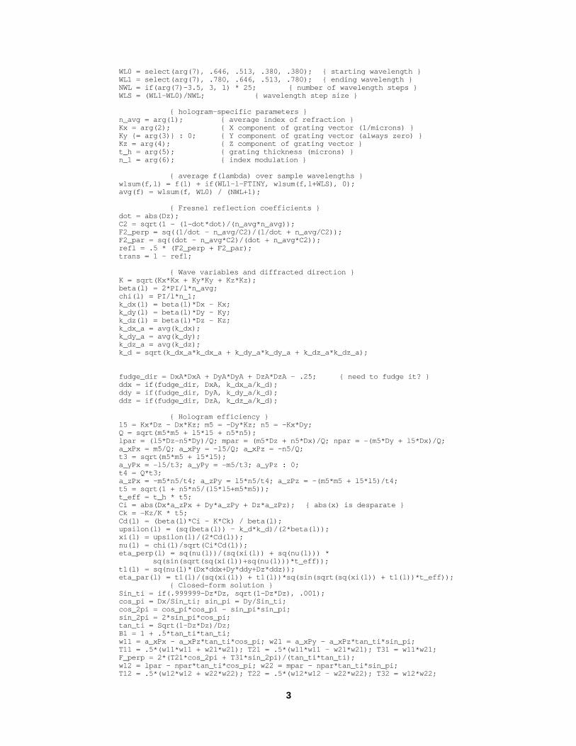
This subroutine is the same as the diffract.cal, except that it computes an average diffraction direction andefficiency over a selected wavelength range, rather than a single, discrete wavelength.
{Diffraction equation for grating without diffuser.
Grating surface is in the X-Y plane, with grating alignedalong the Y axis (i.e. rays are bent in X by grating).
Taken from formulas provided by Physical Optics Corporation.Contact Indra Tengara (310) 320-3088 or (909) 396-0333.
Input parameters:
A1 - average index of refractionA2, A3, A4 - X, Y, Z of grating vector (1/microns)A5 - thickness of grating (microns)A6 - index modulation magnitudeA7 - color component (1=Red,2=Green,3=Blue,4=grey)
Computed values:
dc - diffracted component coefficientddx, ddy, ddz - diffracted component directiontc - transmitted component coefficienttdx, tdy, tdz - transmitted component direction
}
3
WL0 = select(arg(7), .646, .513, .380, .380); { starting wavelength }WL1 = select(arg(7), .780, .646, .513, .780); { ending wavelength }NWL = if(arg(7)-3.5, 3, 1) * 25; { number of wavelength steps }WLS = (WL1-WL0)/NWL; { wavelength step size }
{ hologram-specific parameters }n_avg = arg(1); { average index of refraction }Kx = arg(2); { X component of grating vector (1/microns) }Ky {= arg(3)} : 0; { Y component of grating vector (always zero) }Kz = arg(4); { Z component of grating vector }t_h = arg(5); { grating thickness (microns) }n_1 = arg(6); { index modulation }
{ average f(lambda) over sample wavelengths }wlsum(f,l) = f(l) + if(WL1-l-FTINY, wlsum(f,l+WLS), 0);avg(f) = wlsum(f, WL0) / (NWL+1);
{ Fresnel reflection coefficients }dot = abs(Dz);C2 = sqrt(1 - (1-dot*dot)/(n_avg*n_avg));F2_perp = sq((1/dot - n_avg/C2)/(1/dot + n_avg/C2));F2_par = sq((dot - n_avg*C2)/(dot + n_avg*C2));refl = .5 * (F2_perp + F2_par);trans = 1 - refl;
{ Wave variables and diffracted direction }K = sqrt(Kx*Kx + Ky*Ky + Kz*Kz);beta(l) = 2*PI/l*n_avg;chi(l) = PI/l*n_1;k_dx(l) = beta(l)*Dx - Kx;k_dy(l) = beta(l)*Dy - Ky;k_dz(l) = beta(l)*Dz - Kz;k_dx_a = avg(k_dx);k_dy_a = avg(k_dy);k_dz_a = avg(k_dz);k_d = sqrt(k_dx_a*k_dx_a + k_dy_a*k_dy_a + k_dz_a*k_dz_a);
fudge_dir = DxA*DxA + DyA*DyA + DzA*DzA - .25; { need to fudge it? }ddx = if(fudge_dir, DxA, k_dx_a/k_d);ddy = if(fudge_dir, DyA, k_dy_a/k_d);ddz = if(fudge_dir, DzA, k_dz_a/k_d);
{ Hologram efficiency }l5 = Kx*Dz - Dx*Kz; m5 = -Dy*Kz; n5 = -Kx*Dy;Q = sqrt(m5*m5 + l5*l5 + n5*n5);lpar = (l5*Dz-n5*Dy)/Q; mpar = (m5*Dz + n5*Dx)/Q; npar = -(m5*Dy + l5*Dx)/Q;a_xPx = m5/Q; a_xPy = -l5/Q; a_xPz = -n5/Q;t3 = sqrt(m5*m5 + l5*l5);a_yPx = -l5/t3; a_yPy = -m5/t3; a_yPz : 0;t4 = Q*t3;a_zPx = -m5*n5/t4; a_zPy = l5*n5/t4; a_zPz = -(m5*m5 + l5*l5)/t4;t5 = sqrt(1 + n5*n5/(l5*l5+m5*m5));t_eff = t_h * t5;Ci = abs(Dx*a_zPx + Dy*a_zPy + Dz*a_zPz); { abs(x) is desparate }Ck = -Kz/K * t5;Cd(l) = (beta(l)*Ci - K*Ck) / beta(l);upsilon(l) = (sq(beta(l)) - k_d*k_d)/(2*beta(l));xi(l) = upsilon(l)/(2*Cd(l));nu(l) = chi(l)/sqrt(Ci*Cd(l));eta_perp(l) = sq(nu(l))/(sq(xi(l)) + sq(nu(l))) *
sq(sin(sqrt(sq(xi(l))+sq(nu(l)))*t_eff));t1(l) = sq(nu(l)*(Dx*ddx+Dy*ddy+Dz*ddz));eta_par(l) = t1(l)/(sq(xi(l)) + t1(l))*sq(sin(sqrt(sq(xi(l)) + t1(l))*t_eff));
{ Closed-form solution }Sin_ti = if(.999999-Dz*Dz, sqrt(1-Dz*Dz), .001);cos_pi = Dx/Sin_ti; sin_pi = Dy/Sin_ti;cos_2pi = cos_pi*cos_pi - sin_pi*sin_pi;sin_2pi = 2*sin_pi*cos_pi;tan_ti = Sqrt(1-Dz*Dz)/Dz;B1 = 1 + .5*tan_ti*tan_ti;w11 = a_xPx - a_xPz*tan_ti*cos_pi; w21 = a_xPy - a_xPz*tan_ti*sin_pi;T11 = .5*(w11*w11 + w21*w21); T21 = .5*(w11*w11 - w21*w21); T31 = w11*w21;F_perp = 2*(T21*cos_2pi + T31*sin_2pi)/(tan_ti*tan_ti);w12 = lpar - npar*tan_ti*cos_pi; w22 = mpar - npar*tan_ti*sin_pi;T12 = .5*(w12*w12 + w22*w22); T22 = .5*(w12*w12 - w22*w22); T32 = w12*w22;

4
F_par = 2*(T22*cos_2pi + T32*sin_2pi)/(tan_ti*tan_ti);eperpc = F_perp + (T11 - F_perp*B1)*dot;eparc = F_par + (T12 - F_par*B1)*dot;eta_avg_l(l) = eta_perp(l)*eperpc + eta_par(l)*eparc;eta_avg = avg(eta_avg_l);
{ Diffraction efficiency }dc = trans * eta_avg;
{ Transmitted component }tdx = Dx; tdy = Dy; tdz = Dz;tc = trans * (1 - eta_avg);
UD\LQLW�FDO
This subroutine computes the standard initialization file for the RADIANCE procedural input.
{ SCCSid "@(#)rayinit.cal 2.10 2/29/96 LBL" }
{Initialization file for Radiance.
The following are predefined:
Dx, Dy, Dz - ray directionNx, Ny, Nz - surface normalPx, Py, Pz - intersection pointT - distance from startTs - single ray (shadow) distanceRdot - ray dot productS - world scaleTx, Ty, Tz - world originIx, Iy, Iz - world i unit vectorJx, Jy, Jz - world j unit vectorKx, Ky, Kz - world k unit vectorarg(n) - real arguments, arg(0) is count
For brdf functions, the following are also available:
NxP, NyP, NzP - perturbed surface normal RdotP - perturbed ray dot product CrP, CgP, CbP - perturbed material color
For prism1 and prism2 types, the following are available:
DxA, DyA, DzA - direction to target light source
Library functions:
if(a, b, c) - if a positive, return b, else c
select(N, a1, a2, ..) - return aN
sqrt(x) - square root function
sin(x), cos(x), tan(x),asin(x), acos(x),atan(x), atan2(y,x) - standard trig functions
floor(x), ceil(x) - g.l.b. & l.u.b.
exp(x), log(x), log10(x) - exponent and log functions
erf(z), erfc(z) - error functions
rand(x) - pseudo-random function (0 to 1)
hermite(p0,p1,r0,r1,t) - 1-dimensional hermite polynomial
noise3(x,y,z), noise3a(x,y,z),noise3b(x,y,z), noise3c(x,y,z) - noise function with gradient (-1 to 1)
fnoise3(x,y,z) - fractal noise function (-1 to 1)

5
}
{ Backward compatibility }AC = arg(0);A1 = arg(1); A2 = arg(2); A3 = arg(3); A4 = arg(4); A5 = arg(5);A6 = arg(6); A7 = arg(7); A8 = arg(8); A9 = arg(9); A10 = arg(10);
{ Forward compatibility (?) }D(i) = select(i, Dx, Dy, Dz);N(i) = select(i, Nx, Ny, Nz);P(i) = select(i, Px, Py, Pz);noise3d(i,x,y,z) = select(i, noise3a(x,y,z), noise3b(x,y,z), noise3c(x,y,z));
{ More robust versions of library functions }bound(a,x,b) : if(a-x, a, if(x-b, b, x));Acos(x) : acos(bound(-1,x,1));Asin(x) : asin(bound(-1,x,1));Atan2(y,x) : if(x*x+y*y, atan2(y,x), 0);Exp(x) : if(-x-100, 0, exp(x));Sqrt(x) : if(x, sqrt(x), 0);
{ Useful constants }PI : 3.14159265358979323846;DEGREE : PI/180;FTINY : 1e-7;
{ Useful functions }and(a,b) : if( a, b, a );or(a,b) : if( a, a, b );not(a) : if( a, -1, 1 );abs(x) : if( x, x, -x );sgn(x) : if( x, 1, if(-x, -1, 0) );sq(x) : x*x;max(a,b) : if( a-b, a, b );min(a,b) : if( a-b, b, a );inside(a,x,b) : and(x-a,b-x);frac(x) : x - floor(x);mod(n,d) : n - floor(n/d)*d;tri(n,d) : abs( d - mod(n-d,2*d) );linterp(t,p0,p1) : (1-t)*p0 + t*p1;
noop(v) = v;clip(v) = bound(0,v,1);noneg(v) = if(v,v,0);red(r,g,b) = if(r,r,0);green(r,g,b) = if(g,g,0);blue(r,g,b) = if(b,b,0);grey(r,g,b) = noneg(.265074126*r + .670114631*g + .064811243*b);clip_r(r,g,b) = bound(0,r,1);clip_g(r,g,b) = bound(0,g,1);clip_b(r,g,b) = bound(0,b,1);clipgrey(r,g,b) = min(grey(r,g,b),1);
dot(v1,v2) : v1(1)*v2(1) + v1(2)*v2(2) + v1(3)*v2(3);cross(i,v1,v2) : select(i, v1(2)*v2(3) - v1(3)*v2(2),
v1(3)*v2(1) - v1(1)*v2(3),v1(1)*v2(2) - v1(2)*v2(1));
fade(near_val,far_val,dist) = far_val +if (16-dist, (near_val-far_val)/(1+dist*dist), 0);
bezier(p1, p2, p3, p4, t) = p1 * (1+t*(-3+t*(3-t))) +p2 * 3*t*(1+t*(-2+t)) +p3 * 3*t*t*(1-t) +p4 * t*t*t ;
bspline(pp, p0, p1, pn, t) = pp * (1/6+t*(-.5+t*(.5-1/6*t))) +p0 * (2/3+t*t*(-1+.5*t)) +p1 * (1/6+t*(.5+t*(.5-.5*t))) +pn * (1/6*t*t*t) ;
turbulence(x,y,z,s) = if( s-1.01, 0, abs(noise3(x/s,y/s,z/s)*s) +turbulence(x,y,z,2*s) );
turbulencea(x,y,z,s) = if( s-1.01, 0,

6
sgn(noise3(x/s,y/s,z/s))*noise3a(x/s,y/s,z/s) +turbulencea(x,y,z,2*s) );
turbulenceb(x,y,z,s) = if( s-1.01, 0,sgn(noise3(x/s,y/s,z/s))*noise3b(x/s,y/s,z/s) +turbulenceb(x,y,z,2*s) );
turbulencec(x,y,z,s) = if( s-1.01, 0,sgn(noise3(x/s,y/s,z/s))*noise3c(x/s,y/s,z/s) +turbulencec(x,y,z,2*s) );
{ Normal distribution from uniform range (0,1) }
un2`private(t) : t - (2.515517+t*(.802853+t*.010328))/(1+t*(1.432788+t*(.189269+t*.001308))) ;
un1`private(p) : un2`private(sqrt(-2*log(p))) ;
unif2norm(p) : if( .5-p, -un1`private(p), un1`private(1-p) ) ;
nrand(x) = unif2norm(rand(x));
{ Local (u,v) coordinates for planar surfaces }crosslen`private = Nx*Nx + Ny*Ny;
{ U is distance from projected Z-axis }U = if( crosslen`private - FTINY,
(Py*Nx - Px*Ny)/crosslen`private,Px);
{ V is defined so that N = U x V }V = if( crosslen`private - FTINY,
Pz - Nz*(Px*Nx + Py*Ny)/crosslen`private,Py);
KRORJUDPGHVLJQ
The design of the holographic glazings was determined using the following code.
{ Design a holographic glazing.
10/28/96 Greg Ward}
D : PI/180; { radians per degree }WL : .555; { design wavelength (microns) }n : 1.5; { mean index of refraction for substrate }
{ Input ti and td in degrees: ti - incident angle above horizontal td - diffracted angle above horizontal}
K : 2*PI*n/WL;
{ Output is computed below, zsgn, Kx and Kz: Kx - X-component of gradient vector (always positive) Ky - Y-component of gradient vector (always zero) Kz - Z-component of gradient vector (always positive) zsgn - 1 if Z-axis points into room, -1 if it points out of room}
zsgn = if(ti-td, -1, 1); { reverse Z axis? }
Kx = K * (sin(ti*D) + sin(td*D));Ky : 0; { always zero }Kz = K*zsgn * (cos(ti*D) - cos(td*D));

7
td ti
For ti < td
Z
X
Z
X
For ti > td
Diffracted DirectionIncident Direction
ti →
td →
K →
ti →
td →
K →
By providing the desired ti and td, the resulting Kx and Kz for the simulated wavelength (.555 microns) of lightare then input into the Radiance description of the glazing sample, as shown below:
# Holographic glazing with 50° acceptance and 55.7° diffraction.void prism2 holo3_green13 dc ddx ddy ddz tc tdx tdy tdz diffract.cal -rz 90 -rx -9007 1.5 18.25 0 5.23 10 .029 .555#7 avg_index_of_refraction kx ky kz thick index_modulation_magnitude wavelength_centerholo3_green polygon window0 012 21 31.25 7 21 31.25 9 1 31.25 9 1 31.25 7