design and dynamic modeling of waste stabilization ponds …web.mit.edu/watsan/docs/student...
TRANSCRIPT

Design and Dynamic Modeling of Waste Stabilization Ponds M.Eng. 1999
- 1 -

Design and Dynamic Modeling of Waste Stabilization Ponds M.Eng. 1999
- 2 -

Design and Dynamic Modeling of Waste Stabilization Ponds M.Eng. 1999
- 3 -
Acknowledgements
My deepest gratitude to Professor Donald R. F. Harleman, and to Susan Murcott.
To the Department of Civil and Environmental Engineering of MIT for the possibility to
make such a beautiful trip to Brazil.
Many thanks to Dr. Ricardo Tsukamoto and Dr. Al Pincince for the data and advice they
so graciously supplied.
And to my project partners, Christian Cabral and Domagoj Gotovac.

Design and Dynamic Modeling of Waste Stabilization Ponds M.Eng. 1999
- 4 -
Table of Contents
ABSTRACT .................................................................................................................................................. 2
ACKNOWLEDGEMENTS ......................................................................................................................... 3
TABLE OF CONTENTS............................................................................................................................. 4
LIST OF TABLES........................................................................................................................................ 6
LIST OF FIGURES...................................................................................................................................... 7
CHAPTER 1 - INTRODUCTION .............................................................................................................. 8
CHAPTER 2 - WASTEWATER STABILIZATION PONDS................................................................ 10
INTRODUCTION......................................................................................................................................... 10
WASTEWATER STABILIZATION LAGOONS: A REVIEW .............................................................................. 10
The Advantages of Wastewater Stabilization Ponds ........................................................................... 10
Types of Stabilization Ponds ............................................................................................................... 11
Anaerobic Ponds ............................................................................................................................................. 11
Facultative Ponds ............................................................................................................................................ 13
Maturation Ponds ............................................................................................................................................ 14
DESIGN OF THE LAGOON SYSTEM TO FOLLOW THE CEPT SYSTEM .......................................................... 15
CEPT Settling System Effluent Characteristics .................................................................................. 15
Option 1: Parallel Anaerobic Ponds in Series with Parallel Facultative Ponds ................................ 17
Option 2: Facultative Ponds in Series ................................................................................................ 18
Option 3: Anaerobic pond followed by facultative pond (Restricted area) ........................................ 19
CONCLUSIONS .......................................................................................................................................... 21
CHAPTER 3 - LAGOON MODELING................................................................................................... 22
INTRODUCTION......................................................................................................................................... 22

Design and Dynamic Modeling of Waste Stabilization Ponds M.Eng. 1999
- 5 -
THE FERRARA MODEL.............................................................................................................................. 22
Introduction ........................................................................................................................................ 22
Governing Principles of the Model ..................................................................................................... 23
Adapted Version of the Ferrara Model............................................................................................... 24
MODELING THE RIVIERA DE SÃO LORENÇO DATA ................................................................................... 25
Background......................................................................................................................................... 25
The Riviera Data................................................................................................................................. 27
Riviera Lagoons Loading, Detention Time and removal Efficiencies............................................................. 29
Organic Loading Data ..................................................................................................................................... 33
Inorganic Loading Data................................................................................................................................... 33
Inflow and Outflow Rates ............................................................................................................................... 34
Lagoon Temperature Modeling .......................................................................................................... 34
The Lagoon Temperature Model..................................................................................................................... 38
Sensitivity Analysis for Influent Pond Temperature ....................................................................................... 41
Model Fitting ...................................................................................................................................... 43
The Riviera Anaerobic Pond Model.................................................................................................... 44
Model Sensitivity to Lagoon Temperature...................................................................................................... 46
Modeling the Riviera Facultative Lagoons......................................................................................... 47
Temperature Modeling for the Facultative Pond............................................................................................. 48
Modeling Riviera Facultative Ponds ............................................................................................................... 49
THE JORDAN AERATED LAGOON MODEL ................................................................................................. 51
ASSESSING EFFLUENT QUALITY FROM DESIGN SITUATIONS .................................................................... 57
CHAPTER 4 - CONCLUSIONS AND RECOMMENDATIONS.......................................................... 66
REFERENCES ........................................................................................................................................... 68

Design and Dynamic Modeling of Waste Stabilization Ponds M.Eng. 1999
- 6 -
List of Tables
TABLE 2-1: ANAEROBIC POND DESIGN CRITERIA ......................................................................................... 12
TABLE 2-2: FACULTATIVE POND DESIGN CRITERIA ...................................................................................... 14
TABLE 2-3: MATURATION POND DESIGN CRITERIA ...................................................................................... 15
TABLE 2-4: ESTIMATED CEPT SYSTEM INFLUENT AND EFFLUENT UNDER THREE FLOW REGIMES .............. 16
TABLE 2-5: ANAEROBIC POND DESIGN UNDER THREE LOADING REGIMES................................................... 17
TABLE 2-6: FACULTATIVE POND DESIGN UNDER THREE LOADING REGIMES................................................ 18
TABLE 2-7: PREDICTED EFFLUENT QUALITY FOR OPTION 1.......................................................................... 18
TABLE 2-8: FACULTATIVE POND DESIGN UNDER THREE LOADING REGIMES................................................ 18
TABLE 2-9: PREDICTED EFFLUENT QUALITY FOR OPTION 2.......................................................................... 19
TABLE 2-10: ANAEROBIC POND DESIGN UNDER THREE LOADING REGIMES................................................. 19
TABLE 2-11: FACULTATIVE POND DESIGN UNDER THREE LOADING REGIMES.............................................. 20
TABLE 2-12: PREDICTED EFFLUENT QUALITY FOR OPTION 3........................................................................ 20
TABLE 3-1: LEGEND FOR EQUATIONS 3-1 TO 3-3 .......................................................................................... 24
TABLE 3-2: RIVIERA TEMPERATURE DATA (DR. RICARDO TSUKAMOTO, MONDAY MARCH 8TH 1999)......... 41
TABLE 3-3: PARAMETERS FOR RIVIERA, CORINNE & KILMICHEAL MODELS (20OC) ..................................... 45
TABLE 3-4: MODEL PARAMETER VALUES FOR AS-SAMRA MODEL............................................................... 56
TABLE 3-5: AVERAGE INFLUENT CHARACTERISTICS..................................................................................... 58
TABLE 3-6: PEAK LOADING AND COD REMOVAL AT RIVIERA ANAEROBIC POND........................................ 61
TABLE 3-7: RIVIERA ANAEROBIC POND PEAK-SEASON MODEL PARAMETERS ............................................. 62

Design and Dynamic Modeling of Waste Stabilization Ponds M.Eng. 1999
- 7 -
List of Figures
FIGURE 2-1: PROCESSES INVOLVED IN FACULTATIVE PONDS........................................................................ 13
FIGURE 3-1: RIVIERA DE SÃO LORENÇO TREATMENT SYSTEM SCHEMATIC.................................................. 26
FIGURE 3-2: MONTHLY AVERAGED COD VALUES FOR THE RIVIERA DE SÃO LORENÇO LAGOON SYSTEM... 28
FIGURE 3-3: REMOVAL EFFICIENCY VS. SURFACE LOADING, RIVIERA DE SÃO LORENÇO............................. 30
FIGURE 3-4: COD REMOVAL EFFICIENCY VS. VOLUMETRIC LOADING, RIVIERA ANAEROBIC POND ............ 31
FIGURE 3-5: ANAEROBIC POND COD REMOVAL (EFFLUENT LAGGED BY HRT)........................................... 33
FIGURE 3-6: SCHEMA OF SURFACE HEAT EXCHANGE PROCESSES (CHAPRA, 1997) ...................................... 36
FIGURE 3-7: MODELED TEMPERATURE OF RIVIERA ANAEROBIC LAGOON.................................................... 40
FIGURE 3-8: PLOT OF SENSITIVITY ANALYSIS RESULTS................................................................................ 42
FIGURE 3-9: SCHEMA OF MODEL CALIBRATION PROCEDURE (CHAPRA, 1998) ............................................. 43
FIGURE 3-10: RIVIERA ANAEROBIC LAGOON MODEL ................................................................................... 45
FIGURE 3-11: RIVIERA ANAEROBIC LAGOON MODEL SENSITIVITY TO LAGOON TEMPERATURE .................. 47
FIGURE 3-12: MODELED TEMPERATURES FOR FACULTATIVE LAGOON AT RIVIERA DE SÃO LORENÇO......... 48
FIGURE 3-13: MODELED VS. OBSERVED FACULTATIVE POND EFFLUENT AT RIVIERA DE SÃO LORENÇO...... 50
FIGURE 3-14: TREATMENT SCHEME AT AS-SAMRA (ELLER, 1998) ............................................................... 51
FIGURE 3-15: DAILY COD VALUES FOR AS-SAMRA PONDS M1-3 AND M1-4 .............................................. 52
FIGURE 3-16: MONTHLY AVERAGED COD PROFILE FOR AERATED LAGOONS AT AS-SAMRA ...................... 53
FIGURE 3-17: AS-SAMRA AERATED POND MODEL ....................................................................................... 54
FIGURE 3-18: CORRELATION BETWEEN MODELED AND OBSERVED SERIES OF COD EFFLUENT AT AS-SAMRA
............................................................................................................................................................ 55
FIGURE 3-19: MODELED SABESP AERATED LAGOONS & SETTLING TANKS................................................ 58
FIGURE 3-20: MODELED EFFICIENCY OF PROPOSED LAGOONS TO FOLLOW CEPT STAGE............................. 60
FIGURE 3-21: RIVIERA ANAEROBIC POND �PEAK-SEASON� MODEL.............................................................. 63
FIGURE 3-22: PREDICTED EFFLUENT FROM TATUI ANAEROBIC POND........................................................... 64
FIGURE 3-23: PREDICTED EFFLUENT OF REDESIGNED ANAEROBIC POND ..................................................... 65

Design and Dynamic Modeling of Waste Stabilization Ponds M.Eng. 1999
- 8 -
Chapter 1 - Introduction
The treatment and disposal of wastewater in developing countries is of prime importance
for environmental and public health reasons. The simplest method of municipal
wastewater treatment is through the use of waste stabilization ponds or lagoons. Lagoons
are simple earthen basins in which wastewater is treated by the removal of particulate
matter and the biological degradation of settled solids. Waste stabilization ponds rely on
lengthy detention times and environmental factors (wind, solar radiation) for treatment
efficiency.
This report centers on the design of lagoons following a chemically enhanced primary
treatment (CEPT) stage in Tatui, Brazil. The present treatment facilities in Tatui, which
consist of an anaerobic lagoon followed by a facultative lagoon, are over-loaded, and
hence insufficient. There exists a proposed design to replace the existing facilities by
aerated lagoons followed by settling tanks. This design is proposed by the environmental
agency for the state of São Paulo.
The design of the lagoons that will follow the CEPT stage will be done using empirically
derived guidelines found in literature, and subsequently tested using a model previously
fitted on other lagoons in Brazil. The model is an adapted version of a dynamic �bio-geo-
chemical� lagoon model developed by Raymond Ferrara in 1978. The model will also be
modified to model aerated lagoons, in order to predict the efficiency of the SABESP
design.

Design and Dynamic Modeling of Waste Stabilization Ponds M.Eng. 1999
- 9 -
Chapter 2 will introduce lagoons, and review the processes involved in the three main
lagoon types. Chapter 2 will also review literature in terms of empirical design
guidelines. The chapter will conclude by proposing a design for the lagoons to follow the
CEPT stage at Tatui.
Chapter 3 will introduce the Ferrara model, and exhibit the adapted Ferrara model. The
data used to fit the models will be explained, and a model to predict lagoon temperature
will be developed. The models on lagoons and aerated lagoons will be developed and
studied. Finally, chapter 3 will show the results of the use of the models on the proposed
designs.
Chapter 4 will conclude the report and propose recommendations for both the models and
the lagoon design.

Design and Dynamic Modeling of Waste Stabilization Ponds M.Eng. 1999
- 10 -
Chapter 2 - Wastewater Stabilization Ponds
Introduction
The primary purpose of wastewater treatment is the reduction of pathogenic
contamination, suspended solids, oxygen demand and nutrient enrichment. Waste
stabilization ponds are a cheap and effective way to treat wastewater in situations where
the cost of land is not a factor. The goal of this chapter is to review the different types of
waste stabilization ponds. This chapter will also introduce the design of the lagoons for
the CEAGESP treatment plant in Tatui.
Wastewater Stabilization Lagoons: A Review
The Advantages of Wastewater Stabilization Ponds
Conventional treatment of liquid wastes involve the use of energy intensive mechanical
treatment systems, and are the norm in developed countries (Arthur, 1983.) However,
they are not the best option for less developed countries. Indeed, conventional treatment
schemes were developed due to climatic and area constraints. These constraints are often
not the case in developing countries. Moreover, the use of energy intensive mechanisms
is not desirable in less developed countries, where energy supply is not reliable. Further,
conventional treatment facilities require regular high-skilled maintenance, a thing that is
either too expensive or impossible to find in developing countries.
Stabilization ponds offer many advantages over conventional treatment schemes. One of
their most important advantages is their ability to remove pathogens (WHO EMRO

Design and Dynamic Modeling of Waste Stabilization Ponds M.Eng. 1999
- 11 -
Technical Publication No. 10, 1987.) For conventional systems, pathogen removal is only
attained with tertiary treatment, such as the use of maturation ponds or chlorination. In
addition, stabilization pond systems are much less costly, for both capital costs and
maintenance costs. Pond systems are a viable option for both large and small populations.
Moreover, wastewater stabilization ponds exhibit what is known as the �reservoir effect�,
which enables the pond to absorb both organic and hydraulic shock loadings. The
following section will introduce and describe the different types of wastewater
stabilization ponds.
Types of Stabilization Ponds
There are three main types of stabilization ponds: anaerobic, facultative and maturation.
This section will outline the mechanisms involved in the three main types of ponds, and
will describe their loading capacities and efficiencies.
Anaerobic Ponds
Anaerobic ponds, which are lacking oxygen except at a thin layer at the surface, rely
totally on anaerobic digestion to achieve organic removal. Anaerobic digestion is a two-
stage process. The first stage is putrefaction, and the second stage is methanogenesis.
Putrefaction is the bacterial degradation of organic matter into organic acids and new
bacterial cells. In methanogenesis, methanogenic bacteria break down the products of
putrefaction into methane, carbon dioxide, water, ammonia and new bacterial cells.
Anaerobic ponds operate under heavy organic loading rates (usually greater than 100g
BOD/m3.d). Anaerobic ponds thus contain no dissolved oxygen, and algae are only

Design and Dynamic Modeling of Waste Stabilization Ponds M.Eng. 1999
- 12 -
present on a thin film at the surface). The main mechanism of BOD removal in anaerobic
ponds is by sedimentation of settleable solids, and subsequent anaerobic digestion in the
resulting sludge layer. The typical design and efficiency values for anaerobic ponds can
be seen in Table 2-1.
Table 2-1: Anaerobic Pond Design Criteria
Source Optimal Depth [m]
Surface Loading [kg/ha.d]
Detention Time [d]
BOD Removal [%]
TSS Removal
[%]
Optimal Temperature
[C] Metcalfe & Eddy (1993)
2.5 � 5 225 � 560 20 � 50 50 � 85 20 � 60 30
WHO EMRO Technical Report No. 10 (1987)
2.5 � 5 > 1,000 5 50 � 70 NA 25 � 30
Lagoon Technology International (1992)
2 � 5 > 3,000 1 � 2 75 NA 25
World Bank Technical Paper No. 7 (1983)
4 4,000 � 16,000
2 NA NA 27 � 30
It is obvious that there is a great range of values for surface loading rates for anaerobic
ponds. It has been widely recognized that this type of design criterion is insufficient for
anaerobic ponds. Indeed, the preferred loading rate design value should be expressed with
respect to volume, and not surface area (Metclafe & Eddy, 1993). The typical value for
volumetric loading rate for an anaerobic pond is 100 � 400 g BOD/m3/day.
Anaerobic ponds are used as the primary stage in the pond treatment process. A primary
facultative pond can, however, replace them. Facultative ponds are discussed in the
following section.

Design and Dynamic Modeling of Waste Stabilization Ponds M.Eng. 1999
- 13 -
Facultative Ponds
Facultative ponds take their name from the facultative bacteria that populate them.
Facultative bacteria are capable of adaptive response to aerobic and/or anaerobic
conditions. Facultative ponds degrade organic matter through different processes
depending on the depth layer considered. Figure 2-1 presents a schematic of the processes
involved in facultative ponds.
Figure 2-1: Processes involved in Facultative Ponds
As can be seen in Figure 2-1, facultative ponds have three biologically-active layers. In
the bottom, where sludge accumulates, organic matter is degraded anaerobically. In the
top layer, the organic matter is degraded aerobically due to the presence of dissolved
oxygen produced by photosynthesis occurrence in algae. Finally, in the middle layer, the
facultative layer, dissolved oxygen is present some of the time, fed from the upper layer.
The transformations occurring in a facultative pond are generally from biodegradable
organic matter to living organic matter (i.e. algae, bacteria, protozoa, etc.). In their

Design and Dynamic Modeling of Waste Stabilization Ponds M.Eng. 1999
- 14 -
Technical Paper No. 10, the WHO state that the biochemical oxygen demand generated
from living organisms such as algae is not necessarily detrimental to the environment.
Table 2-2 presents the design criteria for facultative ponds. Again, there are some
discrepancies in the literature, but these discrepancies are mostly due to their reference to
different geographic locations, and hence different climatic conditions.
Table 2-2: Facultative Pond Design Criteria
Source Optimal Depth [m]
Surface Loading [kg/ha.d]
Detention Time [d]
BOD Removal [%]
TSS Removal
[%]
Optimal Temperature
[C] Metcalfe & Eddy (1993)
1.2 � 2.5 60 � 200 5 � 30 80 � 95 70 � 80 20
WHO EMRO Technical Report No. 10 (1987)
1.5 � 2 200 � 400 NA 80 NA 20 � 30
Lagoon Technology International (1992)
1 � 2 100 � 400 NA 70 � 80 NA NA
World Bank Technical Paper No. 7 (1983)
1 � 1.8 200 � 600 NA NA NA 15 � 30
Maturation Ponds
Maturation ponds are placed last in the pond treatment system, if they are used at all.
They are very shallow, and generally occupy very large surface areas. Their main
function is the reduction of pathogenic organisms. Maturation ponds are also known to
remove some algae and some nutrients, but this is not their principal function. The
processes by which the pathogens are removed are multiple, and include sedimentation,
lack of food and nutrients, solar ultra-violet radiation, high temperatures and pH, natural
predators, toxins and natural die-off.

Design and Dynamic Modeling of Waste Stabilization Ponds M.Eng. 1999
- 15 -
The general design values and efficiencies of maturation ponds are presented in Table 2-
3.
Table 2-3: Maturation Pond Design Criteria
Source Optimal Depth [m]
Surface Loading [kg/ha.d]
Detention Time [d]
BOD Removal [%]
TSS Removal
[%]
Optimal Temperature
[C] Metcalfe & Eddy (1993)
1 � 1.5 ≤ 17 5 � 20 60 � 80 NA 20
WHO EMRO Technical Report No. 10 (1987)
1 � 1.5 NA 5 � 10 50 � 60 NA NA
Lagoon Technology International (1992)
1 � 1.5 NA NA NA NA NA
World Bank Technical Paper No. 7 (1983)
1.2 � 1.5 NA 5 NA NA NA
Design of the Lagoon System to follow the CEPT System
Having briefly reviewed the various types of wastewater stabilization ponds, the present
task is to select the appropriate lagoon type and size to treat the CEPT settling tank or
lagoon effluent in our proposed design for Tatui, Brazil. This section will present the
approximate CEPT tank effluent characteristics under three different flow regimes
associated with estimated population growth. Subsequently, an appropriate lagoon design
will be proposed, and the estimated effluent quality presented.
CEPT Settling System Effluent Characteristics
The raw influent characteristics to the Tatui-CEAGESP treatment plant, the CEPT
expected removal efficiencies, and the CEPT effluent characteristics are presented in
Table 2-4. The values for predicted flows and influent quality are taken from the 1992

Design and Dynamic Modeling of Waste Stabilization Ponds M.Eng. 1999
- 16 -
SABESP report on the sanitation situation in Tatui, and the values for removal
efficiencies are taken from the jar test data.
Table 2-4: Estimated CEPT System Influent1 and Effluent under Three Flow Regimes
Year Flow [L/s] Influent BOD [kg/d]
Influent TSS [kg/d]
Effluent BOD [kg/d]
Effluent TSS [kg/d]
1995 135 2945 1491.9 1472.5 298.4 2005 161 3843 1779.2 1921.5 355.9 2015 244 5823 2696.5 2911.5 539.3
Given the data of Table 2-4 and a present available lagoon surface area of 5.5 ha, the
following three options are available:
1. Anaerobic pond(s) (in parallel) followed by facultative pond(s) (in parallel).
2. Facultative pond(s) (in series).
It is also necessary to design lagoons that will fit in the area available after using the in-
pond CEPT treatment option (i.e. 4 ha).
3. Anaerobic pond followed by a facultative pond.
These three options are examined in detail in the next two sub-sections.
1 Raw influent is flow and BOD loading are taken from SABESP Edital 1992. Influent TSS is approximated to 130 mg/L. Removal efficiencies are estimated at 50% for BOD and 80% for TSS.

Design and Dynamic Modeling of Waste Stabilization Ponds M.Eng. 1999
- 17 -
Option 1: Parallel Anaerobic Ponds in Series with Parallel Facultative Ponds
Option 1 involves a number of small anaerobic ponds operating in parallel. The necessity
for multiple anaerobic ponds is dictated by the principle that anaerobic ponds only
function properly under minimal loading. Since the effluent loading is predicted to
increase by one third from 2005 to 2015, it is necessary to provide multiple ponds to
accommodate the growing load, while maintaining a minimal load in each pond.
Table 2-5 presents the anaerobic pond volumes required under the three different loading
scenarios.
Table 2-5: Anaerobic Pond Design under Three Loading Regimes
Year BOD Loading [kg/d]
Volumetric Loading [g/m3/d]
Anaerobic Pond Volume Required
[m3]
Number of Ponds (3.5 m depth)
Pond Area [ha]
Detention Time [d]
1995 1,472.5 105 14,000 1 0.4 1.2 2005 1,921.5 137 14,000 1 0.4 1 2015 2,911.5 104 28,000 2 0.4 1.33
The design values for volumetric loading and detention time in Table 2-5 respect the
minimal quantities to achieve anaerobic conditions. The detention time is on the short
side, but given that most of the suspended solids are removed in the CEPT tanks, a
detention time of one day is presumed to be sufficient. Under these conditions, it is
estimated that the anaerobic lagoons will achieve a further 50 % reduction of the BOD
load.
Under option 1, the effluent from the anaerobic ponds will be directed to a facultative
pond. The design for this facultative pond is seen in Table 2-6.
Design and Dynamic Modeling of Waste Stabilization Ponds M.Eng. 1999
- 18 -
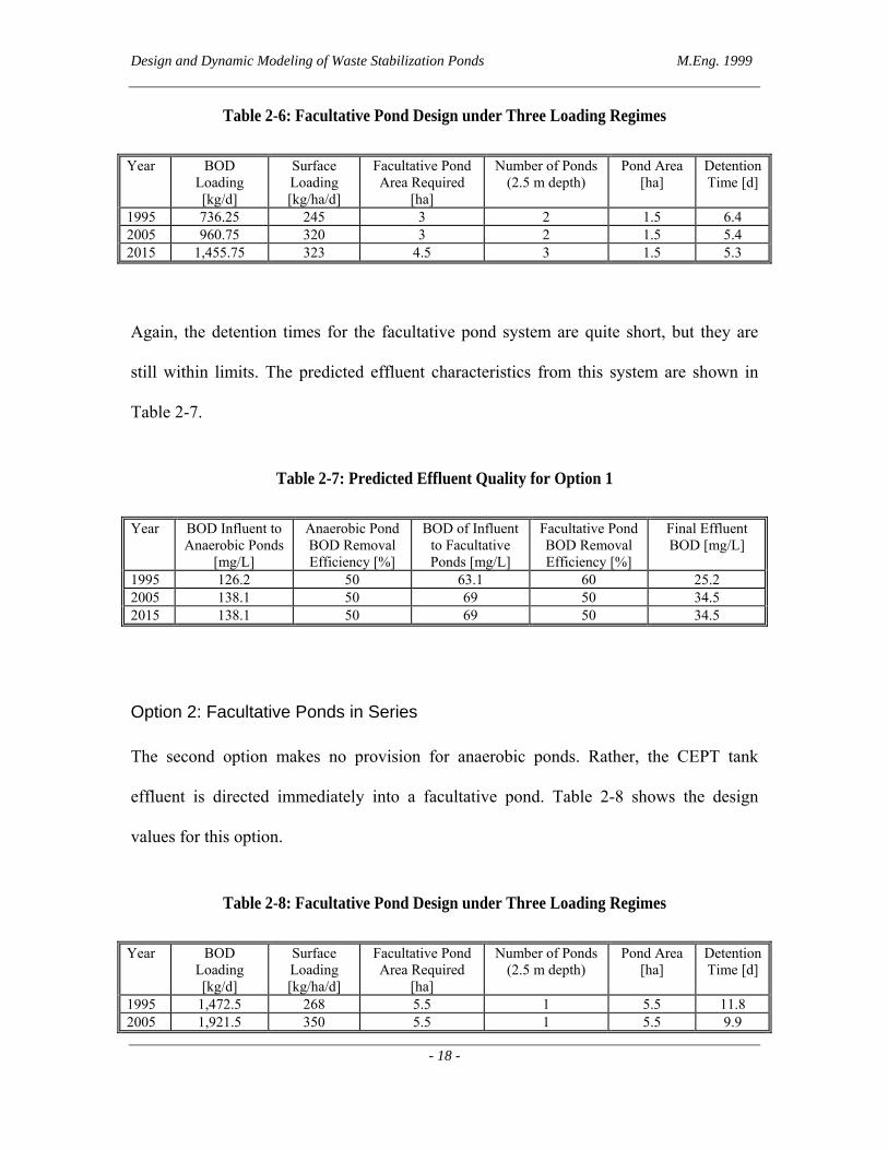
Table 2-6: Facultative Pond Design under Three Loading Regimes
Year BOD Loading [kg/d]
Surface Loading [kg/ha/d]
Facultative Pond Area Required
[ha]
Number of Ponds (2.5 m depth)
Pond Area [ha]
Detention Time [d]
1995 736.25 245 3 2 1.5 6.4 2005 960.75 320 3 2 1.5 5.4 2015 1,455.75 323 4.5 3 1.5 5.3
Again, the detention times for the facultative pond system are quite short, but they are
still within limits. The predicted effluent characteristics from this system are shown in
Table 2-7.
Table 2-7: Predicted Effluent Quality for Option 1
Year BOD Influent to Anaerobic Ponds
[mg/L]
Anaerobic Pond BOD Removal Efficiency [%]
BOD of Influent to Facultative Ponds [mg/L]
Facultative Pond BOD Removal Efficiency [%]
Final Effluent BOD [mg/L]
1995 126.2 50 63.1 60 25.2 2005 138.1 50 69 50 34.5 2015 138.1 50 69 50 34.5
Option 2: Facultative Ponds in Series
The second option makes no provision for anaerobic ponds. Rather, the CEPT tank
effluent is directed immediately into a facultative pond. Table 2-8 shows the design
values for this option.
Table 2-8: Facultative Pond Design under Three Loading Regimes
Year BOD Loading [kg/d]
Surface Loading [kg/ha/d]
Facultative Pond Area Required
[ha]
Number of Ponds (2.5 m depth)
Pond Area [ha]
Detention Time [d]
1995 1,472.5 268 5.5 1 5.5 11.8 2005 1,921.5 350 5.5 1 5.5 9.9

Design and Dynamic Modeling of Waste Stabilization Ponds M.Eng. 1999
- 19 -
2015 2,911.5 530 5.5 1 5.5 6.5
The effluent quality out of the facultative pond is shown in Table 2-9.
Table 2-9: Predicted Effluent Quality for Option 2
Year BOD Influent to Facultative Pond
[mg/L]
Facultative Pond BOD Removal Efficiency [%]
Final Effluent BOD [mg/L]
1995 126.2 70 37.9 2005 138.1 65 48.3 2015 138.1 60 55.2
Option 3: Anaerobic pond followed by facultative pond (Restricted area)
The third option uses less area than the two previous options due to the presence of a
CEPT lagoon, where the chemical coagulation and settling takes place. It is assumed that
the CEPT lagoon will have the same removal efficiencies as the CEPT tanks. This
assumption represents a gross underestimation, since the CEPT lagoons have a hydraulic
retention time (HRT) of 1 day and the CEPT tanks have a HRT of 1 hour.
Table 2-10 presents the design of the anaerobic lagoon under option 3.
Table 2-20: Anaerobic Pond Design under Three Loading Regimes
Year BOD Loading [kg/d]
Volumetric Loading [g/m3/d]
Anaerobic Pond Volume Required
[m3]
Number of Ponds (4 m depth)
Pond Area [ha]
Detention Time [d]
1995 1,472.5 57 26,000 1 0.65 2.2 2005 1,921.5 74 26,000 1 0.65 1.9 2015 2,911.5 112 26,000 1 0.65 1.2

Design and Dynamic Modeling of Waste Stabilization Ponds M.Eng. 1999
- 20 -
The design values for volumetric loading and detention time in Table 2-10 are below the
minimal quantities to achieve anaerobic conditions for years 2005 and 2005. However,
the anaerobic lagoon in Riviera de São Lorenço (refer to chapter on lagoon modeling for
details about Riviera de São Lorenço) exhibited low volumetric loadings, and still
achieved an average 50% removal efficiency. Under these conditions, it is therefore
estimated that the anaerobic lagoons at Tatui will achieve a further 50 % reduction of the
BOD load.
Under option 3, the effluent from the anaerobic ponds will be directed to a facultative
pond. The design for this facultative pond is seen in Table 2-11.
Table 2-11: Facultative Pond Design under Three Loading Regimes
Year BOD Loading [kg/d]
Surface Loading [kg/ha/d]
Facultative Pond Area Required
[ha]
Number of Ponds (3 m depth)
Pond Area [ha]
Detention Time [d]
1995 736.25 223 3.3 1 3.3 8.5 2005 960.75 291 3.3 1 3.3 7.1 2015 1,455.75 441 3.3 1 3.3 4.7
Again, the detention times for the facultative pond system are quite short, but they are
still within limits (c.f. Table 2-2). The predicted effluent characteristics out of this system
are shown in Table 2-12.
Table 2-12: Predicted Effluent Quality for Option 3
Year BOD Influent to Anaerobic Ponds
[mg/L]
Anaerobic Pond BOD Removal Efficiency [%]
BOD of Influent to Facultative Ponds [mg/L]
Facultative Pond BOD Removal Efficiency [%]
Final Effluent BOD [mg/L]
1995 126.2 50 63.1 50 31.5 2005 138.1 50 69 50 34.5 2015 138.1 50 69 50 34.5

Design and Dynamic Modeling of Waste Stabilization Ponds M.Eng. 1999
- 21 -
Conclusions
In this chapter, waste stabilization ponds (lagoons) were reviewed. These lagoons were
shown to have many advantages over more conventional wastewater treatment methods.
The second part of the chapter considered the design of lagoons to follow the chemically
enhanced primary treatment stage for Tatui, Brazil. Three lagoon configuration options
were presented to follow the CEPT stage in Tatui. None of these options was retained as
the �best� option. Indeed, all options produce comparable predicted effluent qualities.
However, the third option is proposed as the one that should kept as the final conceptual
design, because of the reduced area that it occupies. Area constraints are very limiting in
Tatui. Moreover, the third option is suitable for the two possible CEPT applications: in-
tank and in-pond.

Design and Dynamic Modeling of Waste Stabilization Ponds M.Eng. 1999
- 22 -
Chapter 3 - Lagoon Modeling
Introduction
Mathematical modeling not only summarizes accumulated data, but it also provides an
essential analytic tool. Models can act as compact data generators, as well as form the
basic framework for hypothesis testing. Furthermore, models can generate data where it
was absent. Interpolation between data points can be achieved with a model, and so can
extrapolation. In any science, modeling the data is an efficient way to keep a record while
notably increasing its potential usefulness.
Modeling the processes that occur in a waste stabilization pond is an essential part of this
project. Indeed, the model will compare the proposed design with that of a CEPT system
and smaller lagoons. The model will also be useful for lagoon sizing and configuration.
The Ferrara Model
Introduction
The waste-stabilization pond model proposed by Raymond Ferrara describes both
hydraulic transport and biological and chemical transformation of material. The model
was developed in 1978, and was extensively tested on waste stabilization ponds in the
United States. The Ferrara model is a dynamic mathematical model for predicting the
effluent quality of stabilization ponds. Ferrara and Harleman (1981) show that the fully
mixed hydraulic assumption was valid for most waste stabilization ponds. This means
that the underlying hydraulic assumption in the model is that the concentration of all

Design and Dynamic Modeling of Waste Stabilization Ponds M.Eng. 1999
- 23 -
model variables is uniform in the entire pond. The implications of assuming the ponds to
be fully mixed are that the predicted efficiency will be worse than a plug-flow model.
However, the fully mixed assumption ignores dead-zones and short-circuiting.
Governing Principles of the Model
Waste stabilization ponds are an extension of natural systems, and it is therefore
appropriate to use similar modeling approaches. The bio-geo-chemical part of the Ferrara
model is based on five general principles:
1. Mineralization of organic compounds: assumed to be first-order with respect to
organic matter concentration.
2. Organism growth: proportional to organic matter concentration.
3. Net loss of material by settling of non-biodegradable organic matter, precipitation and
adsorption of inorganic phosphorous, and denitrification: assumed to be first-order.
4. Atmospheric re-aeration of CO2: first-order reaction with respect to difference
between saturation and actual concentration of CO2.
5. Removal of fecal coliform by death and predation: assumed to be first-order.
The Ferrara model was developed and tested in 1978 with pond treatment systems in
Corinne, Utah and in Kilmichael, Mississippi.

Design and Dynamic Modeling of Waste Stabilization Ponds M.Eng. 1999
- 24 -
Adapted Version of the Ferrara Model
The complexity of a model is directly related to its accuracy of simulation. However,
complex models need more parameters, and require more sophisticated solution
techniques. The usefulness of a model is dictated by the data available to the modeler. In
our case, the data available and output desired were much related. Indeed, in Brazil, the
main effluent constraints pertaining to environmental legislation revolve around oxygen
demand. There are no legal constraints as to the nutrient or pathogenic contents of
wastewater. The model was therefore restricted to three governing equations. These
equations are Equations 3-1 through 3-3.
( ) ( ) ( ) ( ) ( ) ( )OCICK
ICROCROCROCVQ
OCVQ
dtOCd
SCS
ei
i
+
+−−−= 21112 (3-1)
( ) ( ) ( ) ( ) ( ) ( )OCICK
ICRCOCOROCRICVQ
ICVQ
dtICd
SC
ei
iS
+
−−++−= 21222012 (3-2)
( ) ( ) ( ) ( )FCRFCVQ
FCVQ
dtFCd
Se
ii
8−−= (3-3)
The legend to these equations is presented in Table 3-1.
Table 3-1: Legend for Equations 3-1 to 3-3
SYMBOL DEFINITION OC Concentration of organic carbon IC Concentration of inorganic carbon FC Number of fecal coliforms per unit volume Q Flow rate i Subscript for influent e Subscript for effluent V Volume of pond R12 Transformation rate from organic carbon to inorganic carbon

Design and Dynamic Modeling of Waste Stabilization Ponds M.Eng. 1999
- 25 -
R21 Transformation rate from inorganic carbon to organic carbon R20 Atmospheric re-aeration rate R1S Organic carbon net loss rate KSC Half-saturation constant for carbon R8S Overall fecal coliform decay rate
Reaction rates R12, R21, R1S and R8S are temperature dependent. The value for these
reaction rates is known for a temperature of 20o Celcius. They are corrected to take into
account the lagoon temperature with Equation 3-4.
)20(20 −⋅= TXY
TXY RR θ (3-4)
The three governing equations of the MIT-Ferrara Model were programmed using the
Runge-Kutta 4th Order algorithm for numerical approximation.
Modeling the Riviera de São Lorenço Data
Background
Riviera de São Lorenço is a summer resort located about 140-km northeast of São Paulo.
A private company, Sobloco, manages the water supply and sanitation for Riviera. The
resort-city is fully sewered. The wastewater treatment plant for Riviera is a system of
lagoons. The raw influent is directed through an anaerobic pond, and it is subsequently
directed to one of three facultative ponds (see Figure 3-1 for Riviera de São Lorenço
WWTP schematic.)

Design and Dynamic Modeling of Waste Stabilization Ponds M.Eng. 1999
- 26 -
Figure 3-1: Riviera de São Lorenço Treatment System Schematic
It is widely accepted that the WWTP at Riviera is the best operated in the state of São
Paulo (Personal communication with Dr. Ricardo Tsukamoto, 1999). Moreover, the
lagoons are monitored regularly in terms of water quality and organic-load removal
efficiency. Data from the Riviera de São Lorenço wastewater treatment plant was
obtained through Dr. Ricardo Tsukamoto, who keeps a close contact with the Riviera
staff. The quality and quantity of data available from Riviera are ideal for model-fitting
purposes. Indeed, the Ferrara model had previously only been applied to waste

Design and Dynamic Modeling of Waste Stabilization Ponds M.Eng. 1999
- 27 -
stabilization ponds in the United-States. It was therefore necessary to fit the model to
Brazilian data, before using it in a predictive mode.
Although the characteristics of Riviera and Tatui are entirely different, both treatment
systems under consideration treat domestic waste.
The Riviera Data
The data available from Riviera is of high quality. However, there are some missing
values in the data set. The Ferrara model requires a steady stream of daily values for
organic loading (in the form of concentration of organic carbon), inorganic loading,
inflow rate, outflow rate and pond temperature. None of the latter was complete in the
data set provided. It was therefore necessary to fill the gaps with statistically generated or
modeled data.
The COD removal efficiency of the Riviera lagoon system is depicted in Figure 3-2,
where monthly COD averages are shown for the raw influent, the anaerobic pond effluent
and the combined facultative pond effluent. It should be noted that since the three
facultative ponds are configured in parallel, the monthly COD values were averaged over
the three ponds. These values were computed for a period lasting from the 24th of
December 1997 until the 25th of February 1999.

Design and Dynamic Modeling of Waste Stabilization Ponds M.Eng. 1999
- 28 -
Average Monthly COD for Riviera de Sao Lorenco Lagoon System
100
200
300
400
500
600
700
1 3 5 7 9 11
Month
Influent Anaerobic Pond Effluent Facultative Pond Effluent
Figure 3-2: Monthly Averaged COD values for the Riviera de São Lorenço Lagoon System
The yearly average COD removal efficiency in the anaerobic pond is of 51.4%, whereas
the average facultative pond removal efficiency is of 37.1%. The data that was made
available for the Riviera system represents the period running from the 24th of December
1997 until the 25th of February 1999. The monthly COD averages are therefore only
representative of 1998, except for the months of January and February, which represents
an average of 1998 and 1999. It is important to note that the second facultative lagoon
was undergoing maintenance from the 19th of June to the 17th of December 1998, period
during which it was unused. Also, the third facultative lagoon was only put into service
on the 10th of June 1998, and the first facultative lagoon was not loaded for the months of
June through August, in order to load up the third facultative lagoon. Consequently, the

Design and Dynamic Modeling of Waste Stabilization Ponds M.Eng. 1999
- 29 -
facultative removal efficiency depicted in Figure 3-2 is representative of facultative
lagoons 1 & 2 for the first half of the year, and lagoons 1 & 3 for the second half of the
year. This might explain the low removal efficiencies witnessed in the first half of the
year. The second facultative lagoon, due for maintenance, probably skewed the
efficiencies on the downside. If the first half of the year is omitted in the calculation of
average facultative pond COD removal efficiency, the averaged COD removal is 42.5%
in the facultative lagoons.
Riviera Lagoons Loading, Detention Time and removal Efficiencies
The lagoons at Riviera were examined in terms of organic loading, detention time and
removal efficiency. The objective of this study was to compare the performance of the
lagoons at Riviera with the generic performances cited in the literature.
Figure 3-3 represents the removal efficiencies for all ponds as compared to the surface
loading of the ponds. The three low removal efficiencies that can be seen for the
facultative ponds at low surface loadings are for the months of March, April and May
1998. These are the three months that precede the second facultative pond maintenance
schedule. On the other side, the two highest removal efficiencies for the facultative
ponds, which occur at the same surface loading range, are for the months of September
and November 1998. It is thought that the data available for the Riviera ponds, although
of high quality, is not sufficient to propose firm conclusions. Indeed, the processes that
govern the inner-workings of waste-stabilization ponds are quite complex, being
influenced by climactic, environmental and anthropogenic factors. Thus, a lengthy
dataset is required in order to smooth out the external factors, especially the

Design and Dynamic Modeling of Waste Stabilization Ponds M.Eng. 1999
- 30 -
anthropogenic disturbances (as is the present case). Moreover, the year 1998 is
characterized by many changes in the management of the ponds at Riviera. A new
facultative pond was added, and an existing facultative pond was put in maintenance. It is
therefore suggested that the only valid dataset available from Riviera de São Lorenço is
that of the anaerobic pond, because it was the least subject to anthropogenic
disturbances.
COD Removal Efficiency vs. Surface Loading in Riviera (Anaerobic & Facultative Lagoons)
0%
10%
20%
30%
40%
50%
60%
70%
0 1000 2000 3000 4000 5000 6000 7000
Surface Loading (kg/ha-d)
Facultative Ponds Anaerobic Pond
Figure 3-3: Removal Efficiency vs. Surface Loading, Riviera de São Lorenço
Due to the very low loading of the anaerobic pond, Figure 3-3 presented the anaerobic
pond loading on a surface area basis. During certain periods of very low loading, the
anaerobic pond might act as a facultative pond. It is observed that the anaerobic pond
performs much better than the facultative pond under the same surface loading. However,

Design and Dynamic Modeling of Waste Stabilization Ponds M.Eng. 1999
- 31 -
the anaerobic pond is twice as deep than the facultative ponds (3 m vs 1.5 m). This
enables the anaerobic pond to have a much deeper anaerobic layer when it acts as a
facultative pond, thereby increasing efficiency.
Figure 3-4 presents the anaerobic pond removal efficiency as compared to volumetric
loading. It has been shown in the previous chapter that anaerobic pond loading is best
measured on a volumetric basis and not a surface basis.
Riviera de Sao Lorenco Anaerobic Pond COD Removal Efficiency vs. Loading
35%
40%
45%
50%
55%
60%
65%
0 50 100 150 200 250
Volumetric Pond Loading (g/m3-d)
COD Removal (%)
Figure 3-4: COD Removal Efficiency vs. Volumetric Loading, Riviera Anaerobic Pond
Figure 3-4 exhibits quite a scatter of removal efficiencies. No clear rule can be drawn as
to the relation between loading and removal efficiency. The mean COD removal
efficiency is 50.7%, and the standard deviation about that mean is of 5.8 percentage

Design and Dynamic Modeling of Waste Stabilization Ponds M.Eng. 1999
- 32 -
points. Although the literature cites 100 [g/m3-d] as the minimal loading for an anaerobic
pond to achieve a fully anaerobic state, the data indicates that the present anaerobic pond
achieves quite a regular removal over a range of 25 � 200 [g/m3-d]. The implications of
this are quite interesting. Indeed, if all anaerobic ponds behave similarly, this would
imply that an anaerobic pond could be designed to have a long lifetime, being able to
cope with increased loading. It also implies that the minimum of 100 [g/m3-d] rule can be
foregone.
Figure 3-4 presents the anaerobic pond COD removal that is not lagged by the
appropriate hydraulic retention time. The removal efficiencies lagged by the retention
time are presented in Figure 3-5. The average of the removal efficiencies is 45% and the
standard deviation is 16%. These statistics are biased, however, by some negative
removal efficiencies, which are remnants of the technique used to lag the effluent COD
data by the lag time. Indeed, lag times were calculated on a weekly basis (i.e. related to
weekly average flow), and this might have responsible for negative removals.

Design and Dynamic Modeling of Waste Stabilization Ponds M.Eng. 1999
- 33 -
Riviera Anaerobic Pond COD Removal vs. Loading (Lagged by HRT)
-40%
-20%
0%
20%
40%
60%
80%
0 50 100 150 200 250 300 350 400
Volumetric Loading (g/m3-d)
Figure 3-5: Anaerobic Pond COD Removal (Effluent Lagged by HRT)
Organic Loading Data
Organic loading is measured in terms of concentration of COD and BOD5. On the days
where data was missing, artificial data was generated by linearly interpolating between
two known points. In most cases data was missing for one to three consecutive days. It is
thought that interpolation is acceptable to fill in data for such a small duration.
Inorganic Loading Data
Inorganic loading is necessary for the Ferrara model in terms of inorganic carbon
concentration and carbon dioxide concentration. None of these data were available from

Design and Dynamic Modeling of Waste Stabilization Ponds M.Eng. 1999
- 34 -
Riviera. Indeed, these types of readings are very rarely done in simple WWTPs such as
Riviera. Data points were therefore artificially created to satisfy the model�s needs.
Inflow and Outflow Rates
The flow data available from Riviera presented two problems. First, there were some
days during which no data was available. Second, flow rates were only available into and
out of the whole treatment system. There were no flow rates available for the respective
lagoons.
On the days where flow data was unavailable, points were created by linearly
interpolating between two know points. For the flow rates to and from respective ponds,
the following scheme was developed. Since all inflow enters the anaerobic lagoon, and
the outflow from the anaerobic lagoon is directed to three facultative ponds set in
parallel, the only data point missing is the flow from the anaerobic pond to the facultative
system. Infiltration and evaporation influence the change in flow between lagoons.
Because both infiltration (seepage) and evaporation can be related to the surface area of
the lagoons, and due to the fact that the anaerobic lagoon occupies approximately one
third of the surface area that the facultative ponds occupy (on a use-weighted basis for the
time period), flow rates between the anaerobic pond and the facultative pond were
interpolated one fourth of the way between the inflow and outflow of the whole system.
Lagoon Temperature Modeling
Lagoon temperature is not monitored at all at the Riviera WWTP. It was therefore
necessary to generate temperature data for the lagoons using meteorological data from

Design and Dynamic Modeling of Waste Stabilization Ponds M.Eng. 1999
- 35 -
Santos, a city that lies 50 kilometers south of Riviera. These meteorological data were
obtained from a database maintained by Columbia University, and accessible through the
web at http://ingrid.ldgo.columbia.edu/SOURCES. The following paragraphs will
describe the temperature modeling procedure.
The temperature model is based upon a very simple heat balance for the water body. This
heat balance for a completely-mixed system is expressed in Equation 3-5.
Accumulation = inflow – outflow ± surface heat exchange (3-5)
The term labeled �inflow� represents the heat entering through the inlet stream.
Accordingly, the term labeled �outflow� represents the heat lost through the pond outlet.
The last term, �surface heat exchange� represents the heat gained, or lost, through the air-
water interface of the pond. It should be noted that this model does not take the energy
exchange with sediments into account. The latter can be quite significant in shallow
systems such as lagoons.
The �inflow� and �outflow� terms are described by Equations 3-6 and 3-7.
Inflow = Q*ρ*Cp*Tin(t) (3-6)
Outflow = Q*ρ*Cp*T (3-7)
Where: Q = Flow rate of water coming in the pond or leaving it
ρ = Density of the water
Cp = Heat capacity of water
T = Temperature of water (as function of time for influent temperature)

Design and Dynamic Modeling of Waste Stabilization Ponds M.Eng. 1999
- 36 -
It should be noted that Tin, the temperature of the pond influent, was unavailable. For
modeling purposes, this temperature was assumed to be constant at a value of 25oC (refer
to the sensitivity analysis of the pond influent temperature, for a more detailed discussion
of the ramifications of this assumption).
The surface heat exchange term is a combination of five processes. Figure 3-1 presents a
schema of all processes involved in surface heat exchange. These processes, as seen in
Figure 3-6, can be grouped in two different ways. First, we can distinguish the radiation
versus non-radiation terms, and the second way to group them is to distinguish between
terms that are dependent of the water body temperature or not.
Figure 3-6: Schema of Surface Heat Exchange Processes (Chapra, 1997)
The net surface heat exchange can be represented as
J = Jsn + Jan � (Jbr + Jc + Je) (3-8)
where: Jsn = net solar shortwave radiation
Jan = net atmospheric longwave radiation

Design and Dynamic Modeling of Waste Stabilization Ponds M.Eng. 1999
- 37 -
Jbr = longwave back radiation from the water
Jc = conduction
Je = evaporation
The net shortwave solar radiation is taken from the meteorological data. In the present
case, the closest available weather station that had a good historical record of
meteorological data was Santos, which is located approximately 50 kilometers south of
Riviera de São Lorenço. The rest of the terms from Equation 3-8 can be calculated from
other data, such as wind speed, dry bulb and wet bulb temperatures. It should be noted
that the three latter terms are a function of the pond surface temperature, which is in our
case the unknown. Equations 3-9 through 3-12 represent the terms involved in the surface
heat exchange. The atmospheric longwave radiation is expressed as
Jan = σ*(Tair+273)4*(A+0.031√eair)*(1-RL) (3-9)
(Stefan-Bolzmann Law) (Atmospheric
attenuation)
(Reflection)
where: σ = the Stefan-Bolzmann constant (11.7*10-8 cal (cm2 d K4)-1)
Tair = Air temperature (oC)
A = a coefficient (0.5 to 0.7)
eair = air vapor pressure (mmHg)
RL = reflection coefficient (0.03)
The water longwave radiation term is expressed as

Design and Dynamic Modeling of Waste Stabilization Ponds M.Eng. 1999
- 38 -
Jbr = ε σ * (Ts + 273)4 (3-10)
where: ε = emissivity of water (0.97)
Ts = water surface temperature
The conductive heat transfer is expressed as
Jc = c1 * f(Uw) * (Ts � Tair) (3-11)
where: c1 = Bowen�s coefficient (≈ 0.47 mmHg oC-1)
f(Uw) = dependence of heat transfer on wind velocity = 19 + 0.95 * Uw2
Uw = wind speed as measured at a height of 7m above water surface (ms-1)
The evaporative heat loss can be expressed as
Je = f(Uw) * (es � eair) (3-12)
where: es = saturation vapor pressure at water surface
eair = vapor pressure of overlying air
The saturation and air vapor pressures can be calculated from the surface water
temperature and dry bulb temperature respectively as
e = 4.596 * e (17.27*T / 237.3 + T) (3-13)
The Lagoon Temperature Model
The Ferrara Model used to dynamically predict lagoon effluent quality assumes that the
lagoon is hydraulically fully mixed, and therefore, this assumption will remain for the

Design and Dynamic Modeling of Waste Stabilization Ponds M.Eng. 1999
- 39 -
temperature modeling. Consequently, the water surface temperature term that was
included in the equations in the previous section is analogous to the lagoon temperature.
Also, the data acquired from the web-based database was daily averaged data (a part from
the net solar radiation, which was averaged monthly). Thus, the temperature was modeled
as a daily steady-state phenomenon. This assumption of steady-state implies that the �J�
term on the left-hand-side of Equation 3-8 is set to zero. The remaining equation was
numerically solved to find the lagoon temperature. It should be noted that, as mentioned
before, there was no available data for influent temperature (needed for equation 3-6),
and it was therefore assumed to remain constant at a value of 25oC. A sensitivity analysis
of the resulting lagoon temperature with respect to influent temperature will be provided
later on.
The model results are seen in Figure 3-7.

Design and Dynamic Modeling of Waste Stabilization Ponds M.Eng. 1999
- 40 -
Modeled Lagoon Temperature (Riviera Anaerobic Lagoon)
10
15
20
25
30
35
16-Dec-97 4-Feb-98 26-Mar-98 15-May-98 4-Jul-98 23-Aug-98 12-Oct-98 1-Dec-98
Figure 3-7: Modeled Temperature of Riviera Anaerobic Lagoon
The modeled temperature series has a mean of 22.9oC and a standard deviation of 3oC
about the mean. The maximum-modeled temperature lies at 30.4oC (10th of February
1998), whereas the minimum-modeled temperature is 15.4oC (22nd September 1998).
No validation analysis can be done for the modeled temperature, as there is a complete
absence of data about temperature of lagoons at Riviera de São Lorenço. This is a major
short coming of the model as applied to Riviera. Indeed, it could be argued, and rightly
so, that it is unscrupulous to model the lagoons at Riviera without any possible
subsequent validation of the model. In defense of the approach taken, it could be said that
the time constraints of the M.Eng. thesis are limiting, and therefore the scientific rigors of
mathematical modeling should be relaxed for the purpose of this exercise.
Design and Dynamic Modeling of Waste Stabilization Ponds M.Eng. 1999
- 41 -
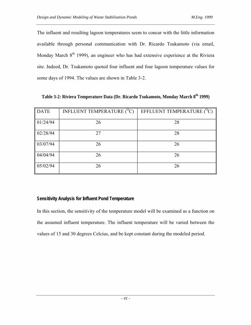
The influent and resulting lagoon temperatures seem to concur with the little information
available through personal communication with Dr. Ricardo Tsukamoto (via email,
Monday March 8th 1999), an engineer who has had extensive experience at the Riviera
site. Indeed, Dr. Tsukamoto quoted four influent and four lagoon temperature values for
some days of 1994. The values are shown in Table 3-2.
Table 3-2: Riviera Temperature Data (Dr. Ricardo Tsukamoto, Monday March 8th 1999)
DATE INFLUENT TEMPERATURE (OC) EFFLUENT TEMPERATURE (OC)
01/24/94 26 28
02/28/94 27 28
03/07/94 26 26
04/04/94 26 26
05/02/94 26 26
Sensitivity Analysis for Influent Pond Temperature
In this section, the sensitivity of the temperature model will be examined as a function on
the assumed influent temperature. The influent temperature will be varied between the
values of 15 and 30 degrees Celcius, and be kept constant during the modeled period.

Design and Dynamic Modeling of Waste Stabilization Ponds M.Eng. 1999
- 42 -
Sensitivity Analysis of Modeled Temperature Series
-20%
-15%
-10%
-5%
0%
5%
10%
15%
15 17 19 21 23 25 27 29
Influent Temperature
Mean of Series Std. Deviation Maximum Minimum
Figure 3-8: Plot of Sensitivity Analysis Results
The plot of the sensitivity analysis (Figure 3-8) shows that the mean, maximum value and
minimum value of the series vary by about 10% when the influent temperature is
increased or decreased by 25% (5oC). The standard deviation of the series varies very
little, by a maximum of 5%. This sensitivity analysis, from which we can conclude that
the model is moderately sensitive to influent conditions, must be complemented by a
sensitivity analysis of the lagoon model with respect to pond temperature. Should the
pond model output vary a lot with temperature, then the choice of influent temperature in
the pond temperature model is significant. The model fitting, discussed in the following
section, will be undertaken using the temperature modeled with a constant 25oC influent.

Design and Dynamic Modeling of Waste Stabilization Ponds M.Eng. 1999
- 43 -
Model Fitting
The model fitting, or calibration process, was done by manual iteration. One of the four
kinetic parameters is changed, and the resulting sum-of-squared errors is evaluated. That
same parameter is changed until the sum-of-squared errors (SSQ) has reached a
minimum. The next parameter is then varied, and the same SSQ minimization is
achieved. The model fitting process is best described by Figure 3-9.
Figure 3-9: Schema of Model Calibration Procedure (Chapra, 1998)
In the iteration process, a second �goodness-of-fit� measure was used: R-square,
comparing modeled and observed series. However, the sum-of-squared error was given
the priority.
Given that the model fitting procedure was manual (i.e. change the parameter, and run the
model), the risks that the fitted model parameters represent a local optimum and not a
global one are great. The models presented in the following sections are the best models
achieved given the time constraints.

Design and Dynamic Modeling of Waste Stabilization Ponds M.Eng. 1999
- 44 -
The Riviera Anaerobic Pond Model
The modified Ferrara model applied to the Riviera de São Lorenço anaerobic lagoon data
is presented in Figure 3-10. Visual inspection of the model reveals that the fit is rather
good. The fitting involved 44 individual iterations of the model, and two iteration-sets for
each parameter. This means that the parameters were optimized one-by-one, and when all
four parameters had been optimized, the process was started again with the newly
optimized values as starting points. Although the total number of iterations pales in
comparison with the number of iterations that would have been accomplished had the
fitting process been computerized, it is thought that the model achieved approaches the
best-possible fit. Indeed, the fitted parameters are extremely close to the parameters for
the Kilmicheal and Corinne ponds that were found by Ferrara in 1978. The fitting process
tried to keep the parameters as close to the Ferrara parameters. This tends to prove that
the modeling framework used is robust. Indeed, if the parameters for ponds in the United
States are similar to those for ponds in Brazil, it tends to prove the validity of the model.

Design and Dynamic Modeling of Waste Stabilization Ponds M.Eng. 1999
- 45 -
Riviera Anaerobic Lagoon
0
100
200
300
400
500
600
700
12/24/97 2/12/98 4/3/98 5/23/98 7/12/98 8/31/98 10/20/98 12/9/98
Date
CO
D (m
g/L)
Observed Effluent of Anaerobic Lagoon Modeled Effluent
Figure 3-20: Riviera Anaerobic Lagoon Model
The final estimated parameters for the Riviera Anaerobic Lagoon Model are shown in
Table 3-3. The Corinne Pond model parameter values were included for comparison
purposes. These are the values that Raymond Ferrara had fit to the first facultative pond
in Corinne (Utah) in 1978.
Table 3-3: Parameters for Riviera, Corinne & Kilmicheal Models (20oC)
PARAMETER Estimated Value for Riviera Anaerobic
Lagoon
Values for First Facultative Pond in
Kilmicheal, MI (Ferrara, 1978)
Values for First Facultative Pond in
Corinne, Utah (Ferrara, 1978)
R12 [day-1] 0.05 0.05 0.05

Design and Dynamic Modeling of Waste Stabilization Ponds M.Eng. 1999
- 46 -
R21 [day-1] 0.02 0.04 0.085
R1S [day-1] 0.04 0.02 0.02
R20 [day-1/m depth] 8.64 8.64 8.64
Model Sensitivity to Lagoon Temperature
The underlying assumption in the lagoon temperature model that the influent temperature
is constant needs to be assessed, as to its consequence on the lagoon model. Figure 3-11
presents the modeled effluent curves for three different lagoon temperature time-series.
The three lagoon temperature time-series are based on the assumptions of constant 20oC,
25oC and 30oC influent.
The models based on the three different influent temperatures are very close to each other
in Figure 3-6. It is concluded that the Riviera de São Lorenço Anaerobic Pond model is
practically not influenced by variations in pond influent temperature, and therefore the
assumption of constant pond influent temperature for the lagoon temperature model is
validated. Indeed, the variations produced by an influent temperature change are not
great, and since it is safe to assume that the temperature of the influent varies between 20
and 30oC, an assumption of a constant 25oC influent is acceptable.

Design and Dynamic Modeling of Waste Stabilization Ponds M.Eng. 1999
- 47 -
Riviera Anaerobic Lagoon Model Temperature Sensitivity
0
100
200
300
400
500
600
12/24/97 2/12/98 4/3/98 5/23/98 7/12/98 8/31/98 10/20/98 12/9/98
CO
D (m
g/L)
Observed Effluent 20oC 25oC 30oC
Figure 3-31: Riviera Anaerobic Lagoon Model Sensitivity to Lagoon Temperature
As previously stated, the anaerobic lagoon at Riviera de São Lorenço is very lightly
loaded in terms of organics. It has been stipulated that this might lead the anaerobic
lagoon to act as a facultative lagoon, with a aerobic layer on the top of the pond profile.
The fitted model will therefore be tested on the facultative lagoons of Riviera by keeping
all the parameters. The only parameter change will occur for R20, which will be scaled for
the different pond depth.
Modeling the Riviera Facultative Lagoons
Riviera de São Lorenço operates three facultative ponds arranged in parallel. For
modeling purposes, it is proposed to model the three facultative lagoons as one lagoon.

Design and Dynamic Modeling of Waste Stabilization Ponds M.Eng. 1999
- 48 -
Indeed, this will greatly simplify the task by ignoring the separation of flow between the
three lagoons, for which no data is available. The temperature model is applied to the
facultative lagoons and other missing data is interpolated as was done for the anaerobic
lagoon. The model developed for the anaerobic pond in Riviera de São Lorenço will be
used in a predictive mode on the �consolidated� facultative pond at Riviera.
Temperature Modeling for the Facultative Pond
To model the facultative pond temperature, the results from the anaerobic pond
temperature model were used as influent temperatures. The facultative pond temperature
model output is show in Figure 3-12.
Modeled Facultative Lagoon Temperature at Riviera de Sao Lorenco
10
15
20
25
30
35
40
45
16-Dec-97 4-Feb-98 26-Mar-98 15-May-98 4-Jul-98 23-Aug-98 12-Oct-98 1-Dec-98
Tem
pera
ture
(oC
)
Figure 3-42: Modeled Temperatures for Facultative Lagoon at Riviera de São Lorenço

Design and Dynamic Modeling of Waste Stabilization Ponds M.Eng. 1999
- 49 -
The modeled series of lagoon temperatures presented in Figure 3-12 has a mean of
22.5oC, a standard deviation about the mean of 5.45oC, a maximum value of 43oC, and a
minimum value of 11oC. The range of the modeled facultative temperature series, which
is of 32oC, is much greater that that of the modeled anaerobic temperature series, which is
of 15oC. This increase in range, and in standard deviation is due to the fact that the
influent temperature is not constant, as it was for the anaerobic pond temperature model.
The plausible errors associated with the constant influent temperature have propagated
onto the temperature model of the facultative pond. However, in the absence of any
validating data, the modeled temperatures for the facultative pond shall be accepted, and
used in the facultative pond model.
Modeling Riviera Facultative Ponds
The temperatures that were modeled for the facultative pond at Riviera de São Lorenço
were input into the adapted version of the Ferrara model. The value for R20 was changed
from 25.92 [day-1] to 12.96 [day-1], to account for the depth of the facultative lagoon,
which is half of the depth of the anaerobic lagoon. Indeed, the rate of loss of inorganic
carbon to the sediment layer is directly related to lagoon depth (Ferrara, 1978).
The modeled facultative ponds of Riviera de São Lorenço are presented in Figure 3-13,
along with the observed effluent quality. The modeled series� basic statistics are close to
those of the observed series. The mean of the modeled series is 139 [mg/L], and that of
the observed series is 162 [mg/L], which represents a difference of 19%. The standard
deviations of the modeled and observed series are 43.8 [mg/L] and 44 [mg/L]
respectively. The model performs poorly at reproducing the shape of the observed series.

Design and Dynamic Modeling of Waste Stabilization Ponds M.Eng. 1999
- 50 -
Indeed, the correlation coefficient between both series is a modest 0.34. Visual inspection
of the modeled and observed series (see Figure 3-13) reveals that the modeled series is an
�exaggerated� version of the observed series. However, the model does seem to capture
the general essence of the observed series. Indeed, the averages of both series are
somewhat close. The model therefore seems to perform well on a general scale without
capturing the details involved.
Riviera de Sao Lorenco Facultative Pond Model Results
0
50
100
150
200
250
300
350
12/24/97 2/12/98 4/3/98 5/23/98 7/12/98 8/31/98 10/20/98 12/9/98 1/28/99
CO
D (m
g/L)
Observed Facultative Effluent Modeled Facultative Effluent
Figure 3-53: Modeled vs. Observed Facultative Pond Effluent at Riviera de São Lorenço
Both the anaerobic pond model and the facultative pond model are deemed suitable for
use as design aids for the lagoons at Tatui. For comparison purposes, a model of an
aerated lagoon followed by a sedimentation tank was developed upon data acquired from

Design and Dynamic Modeling of Waste Stabilization Ponds M.Eng. 1999
- 51 -
Dr. Albert Pincince on the Amman (Jordan) wastewater treatment station. This model
will serve to estimate the performance of the SABESP proposed design.
The Jordan Aerated Lagoon Model
This section presents a model for the aerated lagoons at the As-Samra wastewater
treatment station in Amman, Jordan. As-Samra is the biggest waste-stabilization pond
treatment station in the world, with 187 hectares of waste stabilization ponds designed to
accommodate an average daily flow of 68,000 m3/day. The facilities at As-Samra consist
of three parallel tracks of anaerobic ponds, facultative ponds and maturation ponds in
series. Figure 3-14 presents the schematic of the As-Samra treatment facilities.
Figure 3-64: Treatment Scheme at As-Samra (Eller, 1998)
Figure 3-14 shows that there are four parallel tracks of two anaerobic ponds in series,
followed by three tracks of four facultative ponds and four maturation ponds in series.
The aerated lagoons are ponds M1-3 and M1-4, which are the two last maturation ponds
on the first treatment track. The M1-3 maturation pond is fully-mixed and the M1-4
maturation pond is only partially mixed, to allow for settling (Eller, 1998).

Design and Dynamic Modeling of Waste Stabilization Ponds M.Eng. 1999
- 52 -
The data on the As-Samra treatment system was given by Dr. Albert Pincince, a vice-
president at Camp Dresser Mckee, a consulting firm that had been involved in the
upgrading of the As-Samra treatment facility. It is said that it has been 10 years that the
As-Samra facility was overloaded (Eller, 1998), with an average daily flow in excess of
150,000 m3/day, as compared to the design 68,000 m3/day.
The Data at As-Samra is presented in Figure 3-15, where daily COD values are plotted
for the two-pond system (M1-3 and M1-4).
As-Samra Aerated Pond COD Profiles
0
100
200
300
400
500
600
700
800
900
11-Mar-97 30-Apr-97 19-Jun-97 8-Aug-97 27-Sep-97 16-Nov-97 5-Jan-98 24-Feb-98 15-Apr-98
CO
D (m
g/L)
M1-3 Influent M1-3 Effluent M1-4 Effluent
Figure 3-15: Daily COD Values for As-Samra Ponds M1-3 and M1-4
The influent to M1-3 has a mean of 498 [mg/L] of COD, and its standard deviation is
quite high at 150 [mg/L]. The averaged COD removal efficiency of pond M1-3 is 44%;

Design and Dynamic Modeling of Waste Stabilization Ponds M.Eng. 1999
- 53 -
that of pond M1-4 is 42.7%, and the overall COD removal efficiency of both ponds is
68%.
Figure 3-16 presents the COD loadings averaged on a monthly basis for both ponds.
As-Samra Monthly Averaged Aerated Lagoons COD Profile
0
100
200
300
400
500
600
700
800
Mar-97 Apr-97 Jun-97 Aug-97 Sep-97 Nov-97 Jan-98 Feb-98 Apr-98
CO
D (m
g/L)
M1-3 Influent M1-3 Effluent M1-4 Effluent
Figure 3-16: Monthly Averaged COD Profile for Aerated Lagoons at As-Samra
The effluent requirements are met 50% of the time in terms of BOD5, which is an
effluent concentration of 50 [mg/L]. The colder winter and spring months did not achieve
the effluent requirements.
The aerated maturation ponds have 46 aerators of 37.5 kW each. When the aerators were
installed, the ponds had to be dug deeper to allow for an appropriate detention time; the
resulting depth was of 2.85 meters, for a total pond volume of 153,350 m3.

Design and Dynamic Modeling of Waste Stabilization Ponds M.Eng. 1999
- 54 -
The modified Ferrara Model was applied to the combination of both M1-3 and M1-4
ponds. Indeed, both these ponds form a system. It could be argued that the assumption of
fully-mixed flow is wrong for the combination of these two ponds. However, the model
was fit using that assumption. It was thought that the implications of this error were not
great enough to substantially affect the model. Moreover, by using the fully mixed
assumption, it is implied that both ponds form one inextricable system; and they do: in
the first pond, aeration occurs, and in the second pond the particulate organics settle. This
can be viewed as one system with two steps.
The model was fit using the same procedure as outlined for the anaerobic pond model in
Riviera de São Lorenço. The results of this model-fitting are presented in Figure 3-17.
Jordan Aerated Maturation Pond System
0
50
100
150
200
250
300
350
400
450
500
11-Mar-97 30-Apr-97 19-Jun-97 8-Aug-97 27-Sep-97 16-Nov-97 5-Jan-98 24-Feb-98 15-Apr-98
Observed Series Modelled Series
Figure 3-17: As-Samra Aerated Pond Model

Design and Dynamic Modeling of Waste Stabilization Ponds M.Eng. 1999
- 55 -
The model performed quite well on the Jordan data. Indeed, the modeled series correlates
quite well with the observed series, as can be seen in Figure 3-18.
Correlation of Observed vs. Modelled Series
-0.4
-0.2
0.0
0.2
0.4
0.6
0.8
1.0
0 2 4 6 8 10 12 14 16 18 20
Lag
Cor
rela
tion
Coe
ffici
ent
Figure 3-18: Correlation between Modeled and Observed Series of COD Effluent at As-
Samra
The highest correlation is observed at lag-zero, which means that the modeled effluent is
�synchronized� with the observed effluent quality. The lag-zero correlation coefficient is
quite high at 0.8. Moreover, the �r-squared� value comparing modeled and observed
series is 0.65, which is much higher that the 0.15 value exhibited for the Riviera de São
Lorenço anaerobic pond model. The �r-squared� value is a measure of the linearity of the
relation between the two compared series. In other words, if the modeled values were

Design and Dynamic Modeling of Waste Stabilization Ponds M.Eng. 1999
- 56 -
plotted against their respected observed values, the resulting graph would be a straight
line if the �r-squared� value were one.
The modeled effluent COD converts to a removal efficiency of 59.3% for the two ponds,
whereas the observed effluent represents a removal efficiency of 64.2%. These two
values are quite close, and indicate that the model performed quite satisfactorily.
The fitted-mode parameter values are exhibited in Table 3-4.
Table 3-4: Model Parameter Values for As-Samra Model
PARAMETER AS-SAMRA MODEL
RIVIERA MODEL
CORINNE POND MODEL
R12 [day-1] 0.01 0.05 0.05
R21 [day-1] 0.07 0.02 0.085
R1S [day-1] 0.16 0.04 0.02
R20 [day-1/m depth] 23.86 8.64 8.64
It is interesting to compare all three treatment stations just by observing the parameters
for the modified Ferrara model. Indeed, the Riviera and Corinne models have the greatest
transformation rate from organic to inorganic carbon (R12), whereas the As-Samra model
has the smallest. This would tend to indicate that there is a greater digestion rate of
organic material at Riviera. This makes sense, since the Riviera model is for a lightly
loaded anaerobic pond, where the processes in the lower layer of the pond are all about
organic material digestion. On the other hand, the As-Samra pond model takes its organic
material removal in the R1S parameter, which represents net loss of organic material. The

Design and Dynamic Modeling of Waste Stabilization Ponds M.Eng. 1999
- 57 -
R1S parameter for the As-Samra model is eight times higher than that of the Corinne
pond model, and 4 times higher than that of the Riviera model. The As-Samra model
represents a combination of two ponds, the first one of which is fully mixed, which
means that there is absolutely no settling. The second pond of the As-Samra model is
only partially mixed to allow for settling. The goal of aerated lagoons is to transform the
soluble organic material to particulate organic material, and then to allow it to settle out.
In conclusion, the model worked very well on the As-Samra data. Both the Riviera pond
model and the As-Samra pond model will be used in a predictive mode to assess the
efficiencies of the proposed designed lagoons to follow the chemically enhanced primary
treatment stage at Tatui, and the proposed SABESP aerated lagoon design for Tatui.
Assessing Effluent Quality from Design Situations
The two proposed designs (CEPT & lagoons, Aerated lagoons) for the upgrading of the
CEAGESP treatment facility in Tatui will be assessed in this section. The method used to
assess these designs will be to apply the models that were developed in the previous
sections to the average influent conditions.
The average influent conditions are outlined in Table 3-5. The models will be applied to
these inflow conditions, and the predicted efficiency of the designs will be deducted from
the results of the simulations.

Design and Dynamic Modeling of Waste Stabilization Ponds M.Eng. 1999
- 58 -
Table 3-5: Average Influent Characteristics
Design Lagoons Following CEPT SABESP Aerated Lagoons
Average Influent COD [mg/L] 250 500
Average Flow [L/s] 161 161
The simulation results for the SABESP aerated lagoons and sedimentation tank system
are presented in Figure 3-19.
SABESP Aerated Lagoons Predicted Efficiency
0
100
200
300
400
500
600
0-Jan-00 19-Feb-00 9-Apr-00 29-May-00 18-Jul-00 6-Sep-00 26-Oct-00 15-Dec-00 3-Feb-01
Effluent Influent
Figure 3-79: Modeled SABESP Aerated Lagoons & Settling Tanks
The average removal efficiency found from the As-Samra model, as applied to the
SABESP aerated lagoon design, is 38.2%. This is quite contradictory with the estimated
Design and Dynamic Modeling of Waste Stabilization Ponds M.Eng. 1999
- 59 -
removal efficiency of 95% predicted for the SABESP design. However, the results of this
modeling exercise are not to be taken into consideration, since no attention was given to
the power of the aerators, nor the relative size of the settling tank to the aeration lagoon.
Much more effort has to be given to the aerated lagoon model before it can be used in a
predictive mode. The use of it in this section only serves to underline its imperfection.
To calibrate the model in terms of aeration power, it would be necessary to determine
which of the parameters is affected by the amount of aeration injected into the lagoon.
This could be done by studying one system in depth, observing the variations in effluent
quality with changes in aeration intensity. Moreover, separate models should be
developed for the aeration lagoon and the settling tank. Although they can be accepted as
a system, it is better to separate them, in order to isolate the processes that take place in
the lagoon and in the tank.
The next steps to be taken for the Jordan model are to model the lagoon as a anaerobic
pond with no aeration (the average yearly volumetric loading to the first maturation pond
at As-Samra is 97.5 g/m3-d), and compare the results of this model with those of the
aeration pond model (for the first pond model), and thereby deduce the added efficiency
achieved by aeration. This would permit a crude analysis of the added benefit of aeration,
and possibly could allow for a crude estimate of the aeration coefficient to be included in
the model. Again, it has to be stressed that lack of time and lack of data are the culprits
for the presentation of such a summary study.
The next step is the application of the Riviera model to the lagoons that have been
designed to follow the CEPT stage in the proposed design for the CEAGESP treatment

Design and Dynamic Modeling of Waste Stabilization Ponds M.Eng. 1999
- 60 -
plant in Tatui. Unlike the previous case, this model was fitted on data from a location 160
km east of where it shall be used in a predictive mode. The model was fitted on a facility
of approximately the same size as the one it shall be used on in a predictive mode, and
both treat municipal wastewater excusively.
The results of the simulation on the lagoon system proposed to follow the CEPT stage in
Tatui is presented in Figure 3-20.
Modeled Proposed Lagoons at Tatui (following CEPT Stage)
0
50
100
150
200
250
300
1/0/00 2/19/00 4/9/00 5/29/00 7/18/00 9/6/00 10/26/00 12/15/00 2/3/01
CO
D (m
g/L)
Influent Anaerobic Effluent Facultative Effluent
Figure 3-80: Modeled Efficiency of Proposed Lagoons to follow CEPT stage
The model exhibits an average COD removal of 14.85% for the anaerobic lagoon, and an
efficiency of 40% for the facultative lagoon. The overall efficiency of the modeled
system is 48.75%. These figures are much lower than the predicted values that had been

Design and Dynamic Modeling of Waste Stabilization Ponds M.Eng. 1999
- 61 -
taken from the literature. Indeed, the literature prompted the use of a total efficiency of
75%, which was on the conservative side.
It should be noted that the major difference between the Riviera ponds and those
designed to follow the CEPT stage at Tatui is in the hydraulic retention time (HRT).
Indeed, the yearly averaged HRT for the anaerobic pond in Riviera is 7.5 days, whereas
that of the designed anaerobic pond in Tatui is of 1.9 days. The Facultative ponds at
Riviera have a yearly averaged detention time of 22.5 days, whereas the proposed
facultative ponds for Tatui have a detention time of 7.1 days. There is a factor of about
three between detention times of the Riviera and Tatui lagoons. However, space
constraints in Tatui limited the designed lagoons to their present design retention times.
The population served by the wastewater treatment facilities in Tatui and Riviera are both
around 50,000. However, this population represents the peak loading for Riviera, a
loading that is only experienced in the peak months of January and December. It is during
these two months that the treatment plants at Riviera and Tatui are comparable. The
estimated organic loading of the Tatui treatment station is of 135 g/m3-d of COD,
whereas the peak loading for Riviera lies around 120~200 g/m3-d of COD. Table 3-6
presents the monthly loading and COD removal efficiency for the anaerobic pond at
Riviera.
Table 3-6: Peak Loading and COD Removal at Riviera Anaerobic Pond
MONTH Loading [g/m3-d] Detention Time [d] COD Removal [%] December 97 129 4 54 January 98 121 4 49.4 December 98 202 3 51.4

Design and Dynamic Modeling of Waste Stabilization Ponds M.Eng. 1999
- 62 -
Table 3-6 presents loadings and detention times that are in the range of those expected at
Tatui. Indeed, the average expected loading at Tatui is 135 g/m3-d, and the average
detention time of the designed anaerobic lagoon at Tatui is 2 days. It is therefore expected
that the Tatui anaerobic pond will achieve 50% removal of COD, and not 15% as
predicted by the Riviera model. The cause for the shortcoming of the Riviera model lies
in the seasonal variations in loading of the Riviera treatment system. The model was fit
for the entire year, and not the peak months only. A new model for the peak season is
presented next, and the predictions for the Tatui pond associated with this new model are
also shown. The model predicts an average COD removal for the peak season (December
and January) at Riviera of 44.15%. The observed COD removal during the peak season is
45.25%. the model parameters are seen in table 3-7.
Table 3-7: Riviera Anaerobic Pond Peak-Season Model Parameters
PARAMETER Riviera Peak-Season Model Riviera Year-Round Model R12 [day-1] 0.11 0.05 R21 [day-1] 0.02 0.02 R1S [day-1] 0.04 0.04 R20 [day-1] 8.64 8.64
This model was achieved after 12 iterations, starting with the parameters from the year-
round model. The model results are shown in Figure 3-21.
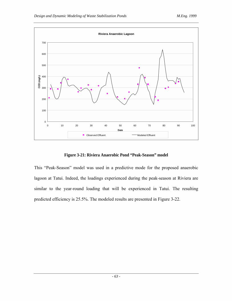
Design and Dynamic Modeling of Waste Stabilization Ponds M.Eng. 1999
- 63 -
Riviera Anaerobic Lagoon
0
100
200
300
400
500
600
700
0 10 20 30 40 50 60 70 80 90 100
Date
Observed Effluent Modeled Effluent
Figure 3-21: Riviera Anaerobic Pond “Peak-Season” model
This �Peak-Season� model was used in a predictive mode for the proposed anaerobic
lagoon at Tatui. Indeed, the loadings experienced during the peak-season at Riviera are
similar to the year-round loading that will be experienced in Tatui. The resulting
predicted efficiency is 25.5%. The modeled results are presented in Figure 3-22.

Design and Dynamic Modeling of Waste Stabilization Ponds M.Eng. 1999
- 64 -
Riviera Anaerobic Lagoon
0
50
100
150
200
250
300
0 10 20 30 40 50 60 70 80 90 100
Date
Influent COD Modeled Effluent
Figure 3-22: Predicted Effluent from Tatui Anaerobic Pond
The models� poor performance is due to the short detention time of the designed
anaerobic lagoon at Tatui. This has prompted a redesign of the anaerobic pond for Tatui.
The newer design provides an anaerobic pond of 1.8 hectares, 4.5 meters deep. This
provides an average detention time of 5.8 days, and the modeled predicted removal
efficiency (using the year-round Riviera anaerobic pond model) can be viewed in Figure
3-23. The average volumetric loading to this redesigned pond is 43g/m3-d. this
volumetric loading was the reason for which the year-round Riviera anaerobic pond
model was used, and the peak-season model. Indeed, the peak-season model was fit onto
data that had an average loading of 150g/m3-d, while the year-round model was fit with
data corresponding to an average loading of 68g/m3-d.

Design and Dynamic Modeling of Waste Stabilization Ponds M.Eng. 1999
- 65 -
Predicted COD Removal Efficiency of Anaerobic Pond at Tatui
30%
35%
40%
45%
50%
55%
60%
11/16/97 1/5/98 2/24/98 4/15/98 6/4/98 7/24/98 9/12/98 11/1/98 12/21/98 2/9/99 3/31/99
% C
OD
Rem
oval
Figure 3-23: Predicted Effluent of Redesigned Anaerobic Pond
The average yearly COD removal efficiency of the redesigned anaerobic pond is 47%.
The variations in removal seen in Figure 3-23 are due to temperature only. Indeed, the
predicted removal efficiencies were derived from the model with constant COD
concentration and flows.

Design and Dynamic Modeling of Waste Stabilization Ponds M.Eng. 1999
- 66 -
Chapter 4 - Conclusions and Recommendations
This report forwarded a design for lagoons to follow a chemically enhanced primary
treatment stage for the city of Tatui in South East Brazil. The preliminary design was
done using empirical guidelines taken from the literature. These empirical design values
are not site specific, and consequently their applicability to various scenarios is
questionable.
It was therefore sought to develop a model that might aid the design process. However,
data short-comings and time restrictions have hindered the development of an
appropriately validated model, useful for the present purpose. The model framework was
taken from Raymond Ferrara�s 1978 doctoral thesis. It had been tried and tested for
facultative ponds in the United-States (South West), and its performance was acceptable
in the predictive mode.
The Ferrara model was simplified to account for the data available in Brazil, and also for
the effluent characteristics that were needed. The model was fit to data from a waste
stabilization pond system on the coast of South West Brazil. The model was also fit on
data acquired from a wastewater treatment station in Amman, Jordan.
The model developed on the Brazilian data was used to predict the effluent quality of the
proposed lagoon design to follow the CEPT stage in Tatui. Results were far below
expectation, and prompted a redesign of the lagoons to follow the CEPT stage. The
redesigned lagoon are shown to achieve the desired removal efficiency.

Design and Dynamic Modeling of Waste Stabilization Ponds M.Eng. 1999
- 67 -
The data that was available for the treatment plant in Jordan was on a sequence of two
aerated lagoons. The first of these lagoons was fully mixed, and the second was only
partially mixed to allow for settling. The model was fit on the combination of both ponds.
That is to say that the two ponds did not have their respective models. The model fit the
data quite beautifully. However, the model did not take the power of aeration into
account, and therefore could not be applied to the proposed SABESP design for Tatui.
The reasons for this obvious shortcoming of the model were lack of data. No relation
could be drawn between aeration intensity and removal efficiency. However, it was
proposed to compare the same lagoon modeled as an anaerobic pond, and compare this
model with the aerated pond model in order to deduce the parameter for aeration power
in the model.