Design and construction of system for sub -20fs pulses through self-phase modulation.

A Thesis Presented

by

Richard Jason Brown

to

The Graduate School

in Partial Fulfillment of the Requirements

for the Degree of

Master of Science

in

Physics

Scientific Instrumentation

Stony Brook University

May 2006

Stony Brook University

The Graduate School

Richard Jason Brown

We, the Thesis committee for the above candidate for the Master of Sciencedegree, hereby recommend acceptance of the Thesis.

Thomas C. Weinacht, Thesis Advisor

Assistant Professor, Department of Physics and Astronomy, Stony Brook

University

Deane Peterson

Professor, Department of Physics and Astronomy, Stony Brook University

James Lukens

Professor, Department of Physics and Astronomy, Stony Brook University

Michael Rijjsenbeek

Professor, Department of Physics and Astronomy, Stony Brook University

This Thesis is accepted by the Graduate School.

ii

Dean of the Graduate School

iii

Abstract of the Thesis

Design and construction of system for sub -20fs pulses through self-phase modulation.

by

Richard Jason Brown

Master of Science

in

Physics

Scientific Instrumentation

Stony Brook University

2006

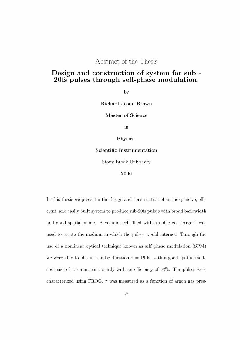
In this thesis we present a the design and construction of an inexpensive, effi-

cient, and easily built system to produce sub-20fs pulses with broad bandwidth

and good spatial mode. A vacuum cell filled with a noble gas (Argon) was

used to create the medium in which the pulses would interact. Through the

use of a nonlinear optical technique known as self phase modulation (SPM)

we were able to obtain a pulse duration τ = 19 fs, with a good spatial mode

spot size of 1.6 mm, consistently with an efficiency of 93%. The pulses were

characterized using FROG. τ was measured as a function of argon gas pres-

iv

sures and pulse energies to find the best combination of both that would yield

the shortest pulse. Results will be further discussed.

v

Contents

List of Figures . . . . . . . . . . . . . . . . . . . . . . . . . . . . . viii

List of Tables . . . . . . . . . . . . . . . . . . . . . . . . . . . . . ix

Acknowledgements . . . . . . . . . . . . . . . . . . . . . . . . . . x

1 Introduction . . . . . . . . . . . . . . . . . . . . . . . . . . . . . . 1

2 Basic principles . . . . . . . . . . . . . . . . . . . . . . . . . . . . 4

2.1 A brief discussion on Gaussian beams . . . . . . . . . . . . . . 4

2.1.1 Beam propagation . . . . . . . . . . . . . . . . . . . . 5

2.1.2 The matrix representation for Gaussian beams . . . . . 6

2.2 Non-Linear optics . . . . . . . . . . . . . . . . . . . . . . . . . 7

2.2.1 Nonlinear Polarization . . . . . . . . . . . . . . . . . . 7

2.2.2 Optical Kerr effect . . . . . . . . . . . . . . . . . . . . 8

2.2.3 Self-phase modulation . . . . . . . . . . . . . . . . . . 10

v

2.3 What is GVD and how do we compensate? . . . . . . . . . . . 12

2.3.1 Some sources of GVD . . . . . . . . . . . . . . . . . . 13

3 Instruments . . . . . . . . . . . . . . . . . . . . . . . . . . . . . . 17

3.1 Cell design . . . . . . . . . . . . . . . . . . . . . . . . . . . . . 17

3.2 How to use the cell . . . . . . . . . . . . . . . . . . . . . . . . 23

3.2.1 Alignment . . . . . . . . . . . . . . . . . . . . . . . . . 23

3.2.2 Pressurizing with argon . . . . . . . . . . . . . . . . . 24

3.3 FROG . . . . . . . . . . . . . . . . . . . . . . . . . . . . . . . 25

4 Results, Calculations, and Characterization . . . . . . . . . . . . 27

4.1 Measurements and results . . . . . . . . . . . . . . . . . . . . 28

4.1.1 Spectra . . . . . . . . . . . . . . . . . . . . . . . . . . 28

4.1.2 Pressure and intensity dependencies . . . . . . . . . . . 32

5 Conclusions and Future Work . . . . . . . . . . . . . . . . . . . . 41

Bibliography . . . . . . . . . . . . . . . . . . . . . . . . . . . . . 44

vi

List of Figures

2.1 Gaussian beam propagation . . . . . . . . . . . . . . . . . . . 6

2.2 Self-phase modulation plot . . . . . . . . . . . . . . . . . . . . 12

2.3 E-field of positively chirped pulse . . . . . . . . . . . . . . . . 15

3.1 design for initial air tests . . . . . . . . . . . . . . . . . . . . . 18

3.2 Project layout . . . . . . . . . . . . . . . . . . . . . . . . . . . 19

3.3 Window mount specification produced with AutoCAD 2006 . 20

3.4 SHG Frog layout . . . . . . . . . . . . . . . . . . . . . . . . . 26

4.1 Amplifier Spectrum . . . . . . . . . . . . . . . . . . . . . . . . 29

4.2 Broadened spectrum . . . . . . . . . . . . . . . . . . . . . . . 31

4.3 Image of beam mode in vacuum . . . . . . . . . . . . . . . . . 35

4.4 The figure illustrates the shape of the beam mode after passing

through the cell. In (a) the mode itself is slightly distorted with

an obvious ring around the mode. (b) shows the horizontal cut

creating a beam profile. . . . . . . . . . . . . . . . . . . . . . . 36

vii

4.5 Image of beam mode in vacuum . . . . . . . . . . . . . . . . . 37

4.6 Pulse duration vs. cell pressure . . . . . . . . . . . . . . . . . 38

4.7 Pulse duration vs. Intensity . . . . . . . . . . . . . . . . . . . 39

4.8 Contour maps of τ . . . . . . . . . . . . . . . . . . . . . . . . 40

viii

List of Tables

3.1 Curved Mirror positioning table. . . . . . . . . . . . . . . . . . 22

ix

Acknowledgements

Write your acknowledgements here...

Chapter 1

Introduction

Stable, mode-locked,and broad bandwidth ultrafast lasers were a revolutionary

introduction in the early 1990’s [1]. Since then, ultrafast lasers have been used

in medical fields [2], ultrafast spectroscopy of semiconductors [3], control of

spectral polarization [4], coherent control [5, 6], Femtochemistry [7, 8],atomic

physics [9], and strong electric field atomic physics [10].

The term ultrafast is generally used to refer to laser pulses of subpicoseond

duration. Commercially available Kerr Lens modelocked titanium sapphire

lasers (an oscillator) are capable of producing pulses with time durations, τ ,

of about 20fs. This meets our demands for pulse duration, but not for peak

pulse power. THe oscillator can produce pulses with energies of about 4nJ

from an averge intensity of 400 mW and a rep rate of about 100 MHz. The

amplifier is used to amplify the pulse energies. The consequence fom using the

1

amplifier is gain narrowing [11]. As the pulse passes through the amplifier there

is a loss in spectral bandwidth and a temporal broadening of τ in time. Pulses

with durations of about 30-35fs and energies of 900µJ-1mJ at a wavelength

λ = 780 nm are typical for our amplified system. These pulse have a rep rate

of about 1 kHz. We need amplified pulses because in our lab we strong field

atomic and molecular physics. If one focuses a 30fs pulse with 1mJ of energy

to a spot size of 10µm, fields on the order of 1011v/m are easily acquired.

The goal of the thesis was to produce an inexpensive, and efficient system to

create sub-20fs pulses and maintain the high pulse energies obtained from the

amplifier. This can be accomplished by using nonlinear optical techniques,

such as self-phase modulation (SPM),detailed in chapter 2, to broaden the

spectral bandwidth after amplification. If the spectral phase of the extended

bandwidth can be controlled, then one can generate pulses with durations

significantly shorter than the pulses directly exiting the amplifier system. Since

we are adding bandwidth to the pulse from SPM, the broadening effect from

dispersive material is amplified. Controlling the phase and compressing the

pulse can be done with chirped mirrors, which are further discussed in chapter

2.

There have been others in the ultrafast field to create this type of system

and have had high success[12, 13]. This one group in particular, Ursula Keller’s

2

group, has been able to obtain pulses as short as 5-7fs through the use of SPM

in a hollow core fiber. While making use of SPM in a hollow core fiber has

been demonstrated to yield pulses as short as 5-7 fs, the efficiency is typically

below 50%, the construction and alignment of the fiber everyday is tedious and

the materials are relatively expensive. We sought an alternative that would be

more efficient, easy to align and inexpensive. This thesis describes the design

construction and testing of an apparatus for producing sub 20 fs amplified

laser pulses through filamentation based self phase modulation in an argon

cell followed by pulse compression using chirped ultrafast laser mirrors

We will move through a basic discussion on the background of the device

in chapter 2, the design and construction of the device in chapter 3, and

measurements and results in chapter 4.

3

Chapter 2

Basic principles

This chapter will cover the basic principles involved. It will present three main

topics: a brief discussion on Gaussian beams, nonlinear effects of self-phase

modulation, and what is Group Velocity Dispersion (GVD) and how do we

compensate?.

2.1 A brief discussion on Gaussian beams

This section will cover some basics on Gaussian beam propagation, and the

calculation of the various parameters used to define Gaussian beams through

the ABCD law.

4

2.1.1 Beam propagation

Here we will describe the propagation of the beam through my system using

Gaussian beam formalism.

The basic Gaussian beam intensity profile for a laser beam has the form

I(x, y, z) ∼ I0e−2(x2+y2)/w(z)2 (2.1)

I0 =1

2ε0cE

20 , (2.2)

where w(z) is the spot size of the beam projected on a screen [14]. There

are various methods used to specify w(z), and must be explicitly stated when

quoting a spot size. For this thesis w(z) will be measured by the 1/e point of

the gaussian beam for the electric field.

We should also consider that the spot size of a laser beam varies with

the distance of propagation. Figure 2.1 shows the shape of the beam as it

propagates a distance in z.

The parameter b is the confocal parameter which is exactly 2z0, where z0

is the Rayleigh range. The Rayleigh range is defined as the point at which the

spot size w(z) of the beam has grown to√

2w0. The spot size at the beam

waist is w0. The divergence of the beam is given by

5

Figure 2.1 As a the beam propagates there is an intrinsic waist associated with

it.

θ =λ

πw0

(2.3)

with

Θ = 2θ (2.4)

and the Rayleigh range

z0 =πw0

λ(2.5)

2.1.2 The matrix representation for Gaussian beams

The matrix formulae Gaussian beams allows us to monitor how the beam is

transformed as it propagates through an optical system. Making use of the

ray matrices used in geometrical optics we have, for our system, three main

optical elements.

The beam first passes through a plano-convex lens into the cell. We can

assume the window on the cell is not contributing to the transformation of

6

the pulse, but just adding phase. The beam then travels a length L through

a medium, in this case argon gas, before bouncing off two curved mirrors

positioned in such a way as to obtain a collimated beam.

After combining the ray matrices found in [14] we can calculate the ray

matrix for our optical system, and it looks as follows.

A B

C D

=

1 0

− 2f3

1

1 L1

0 1

1 0

− 2f2

1

1 L2

0 1

1 0

− 1f1

1

(2.6)

Using the q parameters for gaussian beams, we can relate to our ray matrix,

a beam radius of curvature and a new spot size.

2.2 Non-Linear optics

2.2.1 Nonlinear Polarization

As a light travels through a transparent medium, the electric field field induces

a polarization in that medium. This is the response due to electrons oscillating

inside the medium. In a dielectric medium we have a linear polarizability

P = ε0χE (2.7)

7

where χ = ε − 1 is the electric susceptibility. Relationships for the dis-

placement D, polarization P , and electric field E [15]can be written as

D = εε0E = ε0E + P

P = ε0χE (2.8)

If there exists a medium that elicits a nonlinear response one must take into

account the higher order terms that can be found through a series expansion.

P = ε0[χ(1)E + χ(2)E2 + χ(3)E3 + · · · ] (2.9)

= PL + PNL (2.10)

where χ(1) is the linear term, χ(2) is responsible for second harmonic genera-

tion(SHG) in crystals without inversion symmetry. SHG provides the gating

mechanism for our pulse measurement through Frequency Resolved Optical

Gating (FROG). FROG will be briefly discussed in Chapter 4. The χ(3) term

is responsible for the optical (AC) Kerr effect, nonlinear index of refraction,

self-phase modulation, and self-focussing.

2.2.2 Optical Kerr effect

The optical Kerr effect, also known as the AC Kerr effect, is where a highly

intense beam can create its own modulating electric field. No external field is

8

applied. The electric field can be defined as

E = E0(t)cos(ωt) (2.11)

where E0(t) is the slowly varying envelope amplitude of the electric field which

does not vary substantially over one optical cycle. The equation above if for

the temporal variations of the electric field. If we substitute 2.11 into 2.9 and

ignore all terms except the linear and χ(3) terms we get

P = ε0[χ(1) cos(ωt) + χ(3)E2

0(t) cos3(ωt)]E0(t) (2.12)

= ε0(χ(1) cos(ωt) +

χ3

4E2

0(t)[3 cos(ωt) + cos(3ωt)])E0(t) (2.13)

Equation 2.13 has a ωt term and a 3ωt(third-harmonic generation) term. Ne-

glecting the 3ω term, because it is not of the interest of this thesis, and sim-

plifying shows

P = ε0(χ(1) +

3χ3

4E2

0(t))E0(t) cos(ωt)) (2.14)

As done before for P , χ can be written as

χ = χL + χNL (2.15)

= (χ(1) +3

4χ(3)E0(t)

2) (2.16)

The refractive index for a medium is defined as

n = [1 + χ](12) (2.17)

=√

(ε) (2.18)

9

where from 2.8 above

ε = εL + εNL (2.19)

= (1 + χ(1) +3

4χ(3)) (2.20)

where ε is the dielectric permittivity, and

n =√

εL + εNL ' εL(1 +εNL

2εL

) (2.21)

Now one can arrive at an intensity dependent index of refraction

n = n0 +3χ(3)

8n0

|E0(t)|2 (2.22)

= n0 + n2I(t) (2.23)

2.2.3 Self-phase modulation

If an ultrashort pulse of light travels through a medium, a time varying index

of refraction of the medium from the optical Kerr effect induces a phase shift

in the pulse. This leads to additions to the pulse’s frequency spectrum. The

details of this will be outlined below.

If the electric field in the time-domain is represented as

E(t) = E0 exp (ıϕ(t)) (2.24)

then we can write the phase as

ϕ(t) = ω0t− βz (2.25)

10

where

β =nω0

c(2.26)

where ω0 is the carrier frequency and c is the speed of light in a vacuum.

Substituting for n yields

ϕ(t) = ωt− ω0

c[n0 + n2I(t)]z (2.27)

= ωt− k0z − n2ω0

czI(t) (2.28)

If we separate the linear terms and nonlinear terms, the nonlinear portion of

the phase becomes

ϕNL = −n2ω0

czI(t) (2.29)

We define the instantaneous frequency as

ω =dϕ

dt= ω0 − n2ω0

czdI(t)

dt(2.30)

where the second term in equation 2.30 is the frequency shift induced from

the nonlinear index of refraction.

δω = −n2ω0

czdI(t)

dt(2.31)

Now we have added extra frequency terms in the phase of the E-field giving

E(t) = E0 exp (ı(ω0t− k0z − n2ω0

czI(t))) (2.32)

The nonlinearity introduces new frequency components which allow for

shorter pulse durations than that of the pulse beforehand. However, the phase

11

−60 −40 −20 0 20 40 60−0.5

0

0.5

1

δω

Blue shift

Red shift

Figure 2.2 Self phase modulation on a gaussian pulse. The gaussian shape

is the input pulse. The figure illustrates that as the pulse is rising the is a

frequency shift to the blue, while the frequency shift to the red comes from

the falling edge of the pulse

of these new frequency components needs to be adjusted before the minimum

pulse duration can be attained. This is illustrated in figure... 2.2. This is the

principle that the whole theory is based on.

2.3 What is GVD and how do we compensate?

GVD stands for Group Velocity Dispersion which is the pulse duration of

light spreading in time as the light propagates through a medium. This is a

direct effect of different frequency components in the pulse traveling different

12

velocities while propagating through a dispersive medium.

The spectral phase of the pulse ϕ(ω) is nice to deal with because it allows

one to just add the phase acquired from the different optical components as

the pulse propagates to calculate the total optical phase. We can write ϕ(ω)

as a Taylor expansion around a central frequency ω0 as

ϕ(ω) =∑ 1

n!ϕ(n)(ω0)(ω − ω0)

n (2.33)

which to a second order expansion is

ϕ(ω) = ϕ(ω0) + ϕ′(ω0)(ω − ω0) +1

2ϕ”(ω0)(ω − ω0)

2 + ... (2.34)

The second derivative term ϕ”(ω0) is the only one to have an effect on

pulse shape, if the higher order terms are negligible. We can ignore these

higher order terms because the material dispersion far from resonances can be

described in terms of a Taylor expansion. Thus our GVD is

GV D =1

2ϕ”(ω0)(ω − ω0)

2 (2.35)

2.3.1 Some sources of GVD

The dispersion parameter for a uniform medium is defined as

13

D = −λ

c(d2n

dλ2) (2.36)

ϕ(ω) =ω

cn(ω)D (2.37)

If D ≥ 0 then the medium is said to be anomalously dispersive and add

negative GVD. The pulse becomes negatively chirped. On the other hand

if D ≤ 0 the medium adds positive GVD, thus applying a positive chirp on

the pulse. Most media a pulse travels through has positive dispersion. This

is because we are typically below the resonance frequencies of most optically

transparent materials.

Specialized optics/optical systems need to be developed to provide a neg-

ative chirp if one has an excess of positive GVD from various media and

non-linear optical phenomena. See figure 2.3 for a chirped gaussian pulse

To get the shortest pulse possible precompensation is a method typically

done with the compressor in the amplifier to try to get rid of any GVD the pulse

may see from lenses and other materials before the filament occurs inside the

cell. Unfortunately this method is not useful for GVD that is added from the

formation of the filament on, because of the nonlinear optical phase imprinted

on the pulse in the cell.

Compression is a technique in which the spectral phase of the pulse that

14

−60 −40 −20 0 20 40 60−1

−0.5

0

0.5

1

τ (fs)

E−

field

(a.

u)

Figure 2.3 E-field of a positive, linearly chirped pulse.

exits the cell is flattened. If the spectral phase is completely flat, then the

minimum pulse duration possible is set by the optical spectral bandwidth the

pulse carries. This is known as a ”transform-limited” pulse. Various methods

exist to compress a pulse that are fairly simple to incorporate into ongoing

experiments. Two methods commonly used are a grating compressor and a

Prism Pair Compressor. These methods however were not chosen to compress

the pulse for this project. They were merely mentioned for the realization of

other possible pulse compression options.

Chirped mirrors offer yet another possibility for pulse compression and is

the method of choice for this project. Chirped mirrors are dielectric mirrors in

which the Bragg condition is not constant and varies at different layers with

15

in the structure. So different frequencies penetrate to different extents and

overall see a different group delay. Long wavelengths penetrate deeper into

the structure, and thus see a larger delay. The chirped mirrors used here have

50fs2 per bounce GVD compensation.

If a system has a total positive GVD, then negative GVD can be provided

by chirped mirrors. This method of pulse compression allows for the higher

frequency components, which slow in a positively chirped environment, to

catch up to the lower frequency components. Therefore minimizing the overall

temporal spreading of the pulse in efforts to create a ”transform-limited” pulse.

For a very detailed paper on the theory and design of chirped mirrors see

[16].

As one gets into shorter and shorter pulse durations, more and more at-

tention must be given to any possible pulse spreading.

16

Chapter 3

Instruments

This chapter will cover three main areas. The first will be the design of the

vacuum cell, the second being a brief discussion on how to use the cell, and

finally other instrumentation involved in the project.

3.1 Cell design

The apparatus built as this project is labeled the ”cell”. It is simply a long

hollow vacuum tube filled with an inert gas, with a low dispersion transparent

window on each end to allow the passing of light.

The cell was constructed out of KF-40 vacuum tubing with connections to

allow for vacuum pumping, pressure monitoring, and filling it with argon gas.

Initially tests were done with the nitrogen in the air at atmosphere to

see the filament and obtain spectra using an CCD coupled spectrometer ??.

17

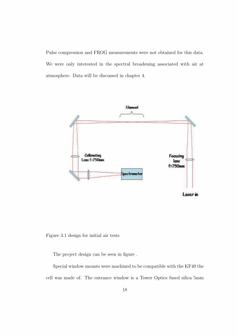
Pulse compression and FROG measurements were not obtained for this data.

We were only interested in the spectral broadening associated with air at

atmosphere. Data will be discussed in chapter 4.

Figure 3.1 design for initial air tests

The project design can be seen in figure .

Special window mounts were machined to be compatible with the KF40 the

cell was made of. The entrance window is a Tower Optics fused silica 5mm

18

Figure 3.2 The filament forms inside the cell generating more colors. The light

is then down collimated with curved optics to decrease the beam spot size.

The pulse is compressed through chirped mirrors before propagating to other

experiments

19

thickness, 1inch diameter window. The design of the window can be seen in

the following figure.

Figure 3.3 Window mount specification produced with AutoCAD 2006

It simply incorporates a 13/16” diameter hole with an o-ring groove cen-

tered 1/8” outside the hole. Since the window is 1” in diameter, the center

of the material for the o-ring needed to lie no further than 1/16” from the

outside edge of the window to provide decent support.

The exit window could not be of the same thickness or material as the

entrance window due to the effects of GVD after the filament. We can prec-

20

ompensate for the material the beam goes through before the filament to pro-

duce a transform limited pulse near the filament, giving us maximum spectral

bandwidth with the amplifier, but not for what comes after. So some caution

needs to be observed about what material we let the beam pass through, and

if that material is going to stretch the pulse out considerably or not. The exit

window available was a 20mm diameter, 250µm thick sapphire window glued

to another blank KF40 end cap. The sapphire window helps minimize the

total GVD on the pulse to make compression easier.

Curved mirrors were used to down collimate the spot size of the beam

and not add GVD to the pulse by going through optics. At the exit of the

cell the spot size is too large to fit enough bounces on chirped mirrors to

provide ample compression of the pulse. We require about four bounces on

each chirped mirror, so we had the to down collimate by a factor of almost

3. The beam is still diverging at the exit window, so curved optics were

placed in such a position as to focus the diverging beam to a suitable spot

size before being collimated. Collimation before down collimation would have

been easier to setup and calculate, but would have also provided some power

losses from the mirrors. The positions and focal lengths of the required optics

were calculated using gaussian beam theory discussed in chapter 2. Table

3.1 is the various curved mirror position parameters with corresponding down

21

CM 1 (mm) CM 2 (mm) DC factor

1400 1656 3.20

1430 1674 2.85

1440 1681 2.80

1460 1696 2.73

1480 1710 2.59

1500 1725 2.50

1600 1803 2.00

Table 3.1 Curved mirrors positions for beam down collimation. The posi-

tion are distance from the focusing lens prior to the cell. CM1 is the first

curved mirror (R=500mm) the beam encounters, while CM2 is the second

(R=-300mm).

collimation factors.

The data seen in table 3.1 is the mirror positions, relative to the initial

focusing lens, for various spot size down collimation factors. down collimating

too much increases the peak intensity of the pulse to a point where various

optical elements could become damaged. So we want to down collimate enough

to work with a varying number of bounces on chirped mirrors, to find the best

pulse compression, and keep any optical elements in the system safe.

22

3.2 How to use the cell

3.2.1 Alignment

Keeping the beam intensity turned down is the safest way to propagate the

beam down to and through the cell. The beam makes several bounces off

mirrors and through a periscope, which can be dangerous even with the power

turned down. This can be adjusted in the amplifier by turning a wave plate.

Making a note of the initial position of the wave plate before making any

changes allow’s one to easily return to the previous settings.

Proper alignment into the cell is critical in that clipping of the beam can

occur very easily on the sapphire exit window. The alignment is performed

using two iris’. One of which is approximately 2.5m from the cell, and the

other is right at the entrance to the cell. This allows for position and angle

alignment forcing the beam to enter straight on and not at some arbitrary an-

gle. Once aligned through the irises, propagation through the cell is allowed.

If one achieved good alignment into the cell, then alignment through the down

collimator and chirped mirrors afterward should be minimal. Caution is ob-

served as to make sure that the beam is not clipping on any of the optics. This

is not only dangerous, but can also result in loss of critical beam intensity and

bad data.

23

3.2.2 Pressurizing with argon

Once the beam is aligned through the cell, and the FROG instrument, then

the cell can be pressurized with argon. The procedure for letting argon in is

somewhat tricky. If not observed, the cell could pressurize to fast to above

atmosphere, and force a leak in the windows. Even worse someone could get

hurt if the window happened to be shot off. The cell is NOT to be pressurized

above 1atm (760 Torr) for experimentation.

First we pump out the cell to roughing vacuum, approximately 10−2 Torr

via a mechanical roughing pump out in the hallway. The vacuum valve on the

cell is usually open when we are not running an experiment. It should only

take 3-5 minutes for the cell to be completely pumped down. Pumping out

the argon line is also necessary because it just allows the vacuum to take out

as much of the air that may be in the system as possible.

Open the main valve on the argon tank next to the regulator pressurizes

the regulator. The black knob on the regulator is the argon gas flow control.

Caution is observed here to not pressurize the cell too fast. Typically one

can allow the argon to flow right into the cell without keeping the inline gas

valve closed, if going up to a few hundred Torr. The convection gauge on

the cell used to measure pressure is not calibrated for argon gas but nitrogen.

There is a calibration curve just above the tank that converts gauge reading to

24

actual pressure inside the cell. Repeating this procedure a few times allows a

more pure sample of argon to enter the cell for the final fill up to the pressure

desired. The back regulator knob is closed once we are done using the argon

Adjusting the pressure once all of the valves are closed is tricky. The

simplest way to increase or decrease the pressure is to open the vacuum valve

on the cell and let some argon out. It is easier to control the pressure if you

have a constant flow through the regulator coming from a lower pressure to a

higher pressure. Typically we drop the pressure first then bring it back up to

the new pressure, and keep all of the valves closed while running an experiment

3.3 FROG

Frequency Resolved Optical Gating is a technique in which ultrashort pulses

can be measured and characterized [17]. The technique is based on Second

Harmonic Generation (SHG) using the pulse to measure itself. It tells us

phase, τ , spectral bandwidth, and symmetry information about the pulse.

Basically the pulse is split in an interferometer, where the pulse from one path

is used as a gate, while the pulse from the other path is the probe and are

recombined in a nonlinear crystal allowing them to interact with each other

with SHG. This means the spectrum recorded on a spectrometer is a ”time-

slice” of the pulse itself. Figure 3.4 is a layout for a SHG FROG system. For

25

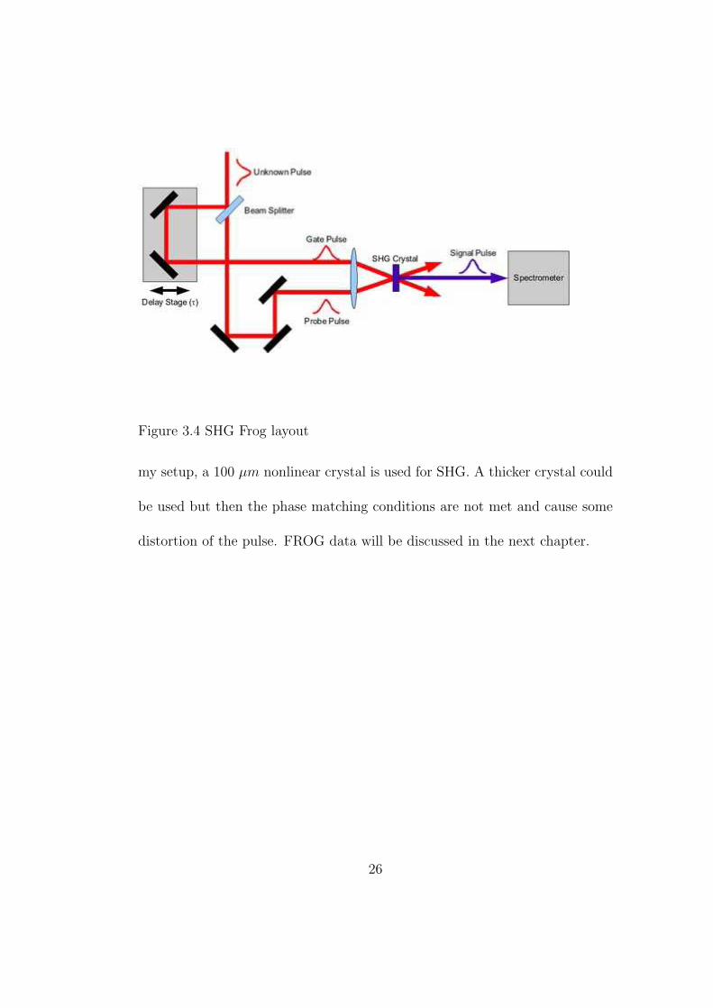
Figure 3.4 SHG Frog layout

my setup, a 100 µm nonlinear crystal is used for SHG. A thicker crystal could

be used but then the phase matching conditions are not met and cause some

distortion of the pulse. FROG data will be discussed in the next chapter.

26

Chapter 4

Results, Calculations, and Characterization

There were three different parameters measured when characterizing this de-

vice, the pulse duration and phase, spectral bandwidth, and mode quality.

These are important measurements because using a pulse with unknown pa-

rameters is not practical. The aim here is to see what conditions must be

met to yield the shortest pulse and to see how sensitively the pulse duration

depends upon argon pressure and peak laser intensity.

The expectation is that we should be able to find some minimum τ as a

function of varying argon pressure and pulse energy. At very low pressure we

should have no SPM, while a high energies we will get some ionization of the

gas forming a plasma that can affect the mode both spatially and temporally.

τ should decrease with increasing pressure up to an atmosphere. SPM should

scale roughly linearly with pressure.

27

4.1 Measurements and results

4.1.1 Spectra

One of the everyday tasks when one routinely brings up the laser is to record

a spectrum out of the amplifier. This lets us know what kind of bandwidth

we have for experimentation. We measure the spectrum by directing a small

portion of the beam into a CCD coupled spectrometer. It is often enough, for

a quick measurement, to take the diffuse light that reflects off of a white card.

The spectrum is used for comparison with cell spectra to see the broadening

difference, as well as a rough measure as to what the shortes possible τ is for

that day. Using a simple LabVIEW program, we can calculate the shortest

possible pulse duration for a given bandwidth. Typically one uses the compres-

sor adjustment in the amplifier to produce the shortest pulse, and so τ for the

spectrum to pulse calculation on the given spectrum is very close to the real τ

that we measure. The actual pulse duration is measured for the amplifier using

the FROG technique discussed in chapter 3 with measurements discussed in

section 4.1.2. A typical spectrum can be seen in figure 4.1 which has about

35nm FWHM of bandwidth and returns a pulse duration of about 28fs. The

spectrum has some noise fluctuations in it, which is mainly due to speckle of

of the white card. Since the card is not a mirror its surface has inconsistencies

28

600 650 700 750 800 850 900 950−0.2

0

0.2

0.4

0.6

0.8

1

1.2S

pect

ral D

ensi

ty

Wavelength

Before Cell

Figure 4.1 Amplifier Spectrum

that cause constructive and destructive interference thus causing the fuzziness

in the amplifier spectrum. Focusing directly into the spectrometer would elim-

inate this. This noise is not real, in the sense that it is not from the laser, so it

is not of great concern. The laser, however, does have some intrinsic noise that

can be characterized by histograms that illustrate how much noise one has in

their system. This noise could have a negative impact on the spectrum that

would exit the cell. The laser noise arises from some fluctuations, in current

and temperature, in the pump laser for the oscillator and from instability in

the mounts in the oscillator. Since we have an output signal that relies on

a nonlinear process to obtain the desired results, this noise tends to become

29

amplified. At this point histograms have not been made for the exit beam of

my cell. However, they are a significant part of the characterization process.

Since the spectrum bandwidth to pulse duration calculation is a not an

actual τ measurement, we can measure the τ we have using FROG. FROG

allows us to completely characterize the ultrashort pulse from the cell in time

from pulse duration to reconstructing the E-field and phase. The FROG re-

construction temporal FWHM, for figure 4.1, τ = 29fs. This shows that the

actual τ is very close to the shortest possible τ , given the spectral bandwidth

we have.

The spectrum seen exiting the cell is substantially broadened with respect

to the amplifier spectrum. This is exactly what we were looking for, because

this broadened spectrum in principle allows to generate a shorter pulse. This

spectrum was acquired using a the maximum pulse energy attainable at the

entrance to the cell (900µJ) and an argon gas pressure of 660 Torr. Argon is

ideal because argon has a high ionization potential, which means the generation

of pulse distorting ions is minimal. This is beneficial because the dispersion

of a plasma can be strong depending on the density. Figure 4.2 shows the

broadened spectrum compared to the amplifier spectrum. One can easily see

that self phase modulation inside the cell causes dramatic broadening of the

spectrum.

30

600 650 700 750 800 850 900 950−0.2

0

0.2

0.4

0.6

0.8

1

1.2S

pect

ral D

ensi

ty

Wavelength

Spectral Broadening in Argon

Before CellAfter Cell

Figure 4.2 Broadened spectrum with a pulse intensity of 900µJ and argon

pressure of 660 Torr

With the input bandwidth of about 35nm we obtain a broadened band-

width of roughly 83nm. The actual bandwidth achieved from the broadening

in the cell is dependent upon pulse energy and argon gas pressure, both dis-

cussed below in section 4.1.2, as well as the position of the compressor in

the amplifier. Before, we adjusted the compressor in the amplifier to achieve

the shortest pulse possible. Now we want to adjust the compressor to maxi-

mize the bandwidth that exits the cell. This in principle precompensates for

any GVD the pulse obtains before the formation of a filament, and places a

”transform-limited” pulse somewhere in the filament, providing as broad of a

31

bandwidth at the output of the cell as possible. The shortest τ possible from

the broadened spectrum is τ = 19.3fs. The next step is to see what is required

to actually attain a pulse this short.

4.1.2 Pressure and intensity dependencies

Cell pressure and pulse intensity play an extremely important role in output

pulse duration. This section will map out how the pressure and intensity affect

the transformation of the pulse.

First, the beam that exits the cell has a large amount of GVD that is

spreading the pulse duration of 19fs out to ' 180fs. This requires compression

from the chirped mirrors discussed in Chapter 3. To compensate for this GVD

we used two chirped mirrors with four bounces per mirror.

The mode of the beam at roughing vacuum (' 10−2 Torr) is very close to

gaussian.

The spot sizes of the modes in figure 4.3 are roughly 1.7 mm at the 1/e

point of the field. This suggests that the mode spot size does not change with

increasing pulse energy and pressure.

After the SPM occurs the beam makes its way out of the cell. We were

concerned about the fact that too high of a pulse energy, would form a plasma

and cause diffraction of the light inside the filament, thus changing the shape of

32

the mode. The mode itself didn’t change, but we now have a very pronounced

ring around the mode. See figure 4.4 below.

Pulse measurements were made using a FROG and reconstructed with

Femtosoft FROG software. The SHG blue light demonstrated in figure 3.4 was

maximized by adjusting the temporal overlap with a mirror on the non-moving

arm. The reconstructions return temporal, spectral, and phase information

about the the pulses. Figure 4.5 are frog reconstructions for I = 800µJ and

pressure P = 720 Torr.

We have obtained a pulse duration of τ ' 19.3fs with a spectral bandwidth

of approximately 71nm after compression.

Pulse measurements were made with FROG by taking six energies at the

entrance of the cell from 500µJ − 950µJ and varying the pressure from 100

Torr - 720 Torr. The intention here was to create a plot to locate the best pos-

sible pressure and energy combination that returns the shortest pulse without

distorting the mode.

First, plots of pulse duration vs. pressure, and pulse duration vs. pulse

energy were created and can be seen in figures 4.6 and 4.7 respectively.

Figure 4.6 shows a decline in τ for an increase in pressure. This suggest

that we should find the shortest pulses at high pressures. The dependence on

pulse energy in the range from 500 to 950 µJ is rather weak, and this is quite

33

beneficial to us because it means that we will be able achieve relatively short

pulses for a large range of pulse energies. Over a range of 450µJ , τ overall

only changes 2− 3fs. This is not a substantial difference in comparison with

how τ depends on argon pressure. The data also suggests that maximizing the

pulse energy is not desirable. This means that if we want to use high energies

we should consider changing the focal geometry by using a longer focal length

lens. This would create a more stable mode, decrease the peak intensity of

the beam (allowing for the high pulse energies), provide frequency broadening

without creating a plasma, and retain the short τ .

Now with figures 4.7 and 4.6 we can construct a surface plot which shows

the dependence of the output pulse duration on pressure and pulse energy. See

figure 4.8.

The graph shows that a minimum seems to exist at low pressures and pulse

energies. Our expectation was that we would find some minimum τ for varying

pressure and energy, and we did. However, for the experiments conducted in

the lab, we need higher pulse energies ( ∼ 800− 900µJ) than the 500µJ that

gives us the shortest τ . The best pressure/pulse energy combination for us is

approximately at 720 Torr and 800 µJ , giving us a compressed τ of 19.3 fs.

34

pixel

pixe

l

200 400 600 800 1000 1200

200

400

600

800

10000.2

0.3

0.4

0.5

0.6

0.7

0.8

0.9

1

(a) a.

(b) b.

Figure 4.3 (a) is the mode of the beam. There is a back reflection off of a ND

filter that can be seen just above the main spot, and (b) is the beam profile in

a vacuum. It has been background subtracted and fit with a gaussian. This

is a line out in the horizontal direction of (a).

35

Pixel

Pix

el

200 400 600 800 1000 1200

200

400

600

800

10000.2

0.4

0.6

0.8

1

(a)

(b)

Figure 4.4 The figure illustrates the shape of the beam mode after passing

through the cell. In (a) the mode itself is slightly distorted with an obvious

ring around the mode. (b) shows the horizontal cut creating a beam profile.

36

−30 −20 −10 0 10 200

0.5

1

Time (fs)

Inte

nsity

−30 −20 −10 0 10 201

1.5

2

2.5

3

3.5

4

Pha

se (

rads

)

(a)

740 760 780 800 820 840 860 8800

0.5

1

λ (nm)

Inte

nsity

740 760 780 800 820 840 860 8800

0.5

1

1.5

2

2.5

Pha

se (

rads

)

(b)

Figure 4.5 We can see in (a) the temporal reconstruction of the pulse while

(b) shows us the spectral reconstruction. These plots show phase on the right

hand side and relative intensity on the left

37

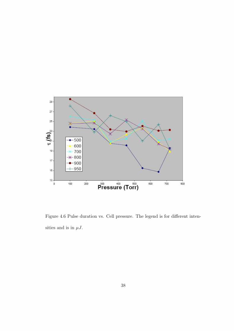
Figure 4.6 Pulse duration vs. Cell pressure. The legend is for different inten-

sities and is in µJ .

38

Figure 4.7 Pulse duration vs. Intensity for different pressures.

39

500 600 700 800 900100

200

300

400

500

600

700

Intensity(mW)

Pre

ssur

e (T

orr)

16

18

20

22

24

26

28

(a)

500600

700800

900200

400600

10

20

30

Pressure (Torr)Energy(µJ)

τ (f

s)

16

18

20

22

24

26

28

(b)

Figure 4.8 (a) is a surface plot of τ with the colorbar on the right showing the

τ scale and (b) is the 3D version to show a slope and a minimum

40

Chapter 5

Conclusions and Future Work

In conclusion we were successful in the design and construction of a system

to produce broad bandwidth, high energy, and reasonably flat phase sub-20

fs pulses that is far more inexpensive and much easier to build and main-

tain than the hollow core fiber setup. We have consistently achieved pulses

with a compressed τ as short as 19 fs with a spectral bandwidth of 70 nm,

and have observed the pressure and pulse energy dependencies on these short

pulses through detailed characterization of this setup. Experiments with the

pulses from this system were not done before the time of this thesis. Through

the characteriztion of the system we have confirmed that our requirements

have bet met for the pulse parameters. These pulses will be used for ongoing

experiments in the area of strong field atomic physics.

41

Bibliography

[1] W. Sibbett” ”D.E. Spence, P.N. Kean. ”60-fs pulse generation from a self-

mode-locked ti:sapphire laser”. ”Optics Letters”, 16(21):1762, November

”1991”.

[2] Aquavella J. Zhao Y. Wang, J. and S. Chung. Tear dynamics mea-

sured with real-time optical coherence tomography. Journal of Vision,

4(11):89a, 2004.

[3] J. Shah. Ultrafast spectroscopy of semiconductors and semiconductor

nanostructures. Springer-Verlag, Berlin, 1996.

[4] Dan; Silberberg Yaron Polachek, Lea; Oron. Full control of the spectral

polarization of ultrashort pulses.

[5] Langchi Zhu, Valeria Kleiman, Xiaonong Li, Shao Ping Lu, Karen Trentel-

man, and Robert J. Gordon. Ultrafast coherent control and destruction

of excitons in quantum wells. Phys. Rev. Lett., 75(13):2598–2601, 1995.

42

[6] T. Hornung, R. Meier, r. de Vivie-Riedle, and M. Motzkus. Coherent con-

trol of the molecular four-wave-mixing response by phase and amplitude

shaped pulses. Chem. Phys., 267:261–276, 2001.

[7] Ahmed H. Zewail J. Spencer Baskin. Ultrafast electron diffraction:

Oriented molecular structures in space and time. ChemPhysChem,

6(11):2261–2276, 2005.

[8] A. Assion, T. Baumert, M. Bergt, T. Brixner, B. Kiefer, V. Seyfried,

M. Strehle, and G. Gerber. Control of chemical reactions by feedback-

optimized phase-shaped femtosecond laser pulses. Science, 282:919–922,

1998.

[9] R. Holzwarth Th. Udem and T. W. Hnsch. Optical frequency metrology.

Nature, 416:233–237, 2002.

[10] Patrick Henning Nurnberger and Thomas Weinacht. Design and con-

struction of an apparatus for the neutral dissociation and ionization of

molecules in an intense laser field. Master’s thesis, Stony Brook Univer-

sity, 2003.

[11] P. Maine ”J.S. Coe and P. Bado”. ”regenerative amplification of picosec-

ond pulses in nd:ylf: gain narrowing and gain saturation”. ”Journal of

the Optical Society of America B”, 5(12):2560–, December ”1988”.

43

[12] S. De Silvestri M. Nisoli and O. Svelto. Generation of high energy 10

fs pulse by a new pulse compression technique. Applied Physics Letters,

68(20):2793–2795, March 1996.

[13] F.W. Helbing A. Heinrich A. Couairon A. Mysyrowicz J. Biegert U. Keller

C.P. Hauri, W. Kornelis. Generation of intense, carrier-envelope phase-

locked few-cycle laser pulses through filamentation. Applied Physics B:

Lasers and Optics, 79:673–677, 2004.

[14] ”Peter W. Milonni and Joseph H. Eberly”. ”LASERS”. ”John Wiley and

Sons”, ”1988”.

[15] Anthony E. Siegman. Lasers. University Science Books, Sausalito, 1986.

[16] ”R. Szipocs and A. Kohzi-Kis”. ”theory and design of chirped dielectric

laser mirrors”. ”Applied Physics B: Lasers and Optics”, 65(2):115–135,

August ”1997”.

[17] Rick Trebino, Kenneth W. DeLong, David N. Fittinghoff, John N.

Sweetser, Marco A. Krumbugel, Bruce A. Richman, and Daniel J. Kane.

Measuring ultrashort laser pulses in the time-frequency domain using

frequency-resolved optical gating. Rev. Sci. Instrum., 68(9):3277–3295,

1997.

44