design and construction of light weight portable …

DESIGN AND CONSTRUCTION OF LIGHT WEIGHT

PORTABLE NMR HALBACH MAGNET

Hung Dang Phuc1, Patrick Poulichet

2, Tien Truong Cong

1, Abdennasser Fakri

2, Christophe Delabie

2,

Latifa Fakri-Bouchet1

Laboratoire CREATIS UMR CNRS 5220, INSERM U1044, INSA de Lyon, Universite de Lyon, Lyon 1

3, rue Victor-Grignard

69616 Villeurbanne, France1

ESIEE, 2 BD Blaise Pascal

93162 Noisy Le Grand, France2

Emails: [email protected], [email protected], [email protected]

Submitted: Sep. 27, 2014 Accepted: Nov. 5, 2014 Published: Dec. 1, 2014

Abstract- A light weight, simple design NMR apparatus consists of 24 identical magnets arranged in

Halbach array was designed and built. The homogeneity of the magnetic field B0 can be improved

by dividing a long magnets into several rings. The size of the useful volume depends on both the gap

between each ring and some others shim magnets. Our aim is to enhance the sensitive volume and

to maintain the highest magnetic static field (B0). This apparatus generates a B0 field strength of

about 0.1 T. This work focuses on the magneto-static simulation of NdFeB magnets arrangement

and on the comparison with the measurement of the magnetic field strength and homogeneity in

three dimensions (3D). The homogeneity of the magnetic field B0 is optimized with the help of CAD

and mathematical software. Our results were also validated with a Finite Element Method (FEM).

The simulation results of the strength and of the homogeneity of B0 field were compared to those

obtained with a digital gaussmeter. The homogeneity in the magnet longitudinal axis and the field

B0 strength are similar. However, the homogeneity in transverse plane differs from simulation and

measurement because of the quality of the magnets. In order to improve the homogeneity, we

propose a new shim method.

Index terms: Nuclear Magnetic Resonance (NMR); Low field; Portable Permanent

Magnet; Halbach; Shim magnets; Homogeneity, Simulation, Finite Element Method

(FEM).

INTERNATIONAL JOURNAL ON SMART SENSING AND INTELLIGENT SYSTEMS VOL. 7, NO. 4, DECEMBER 2014

1555

mailto:[email protected]

mailto:[email protected]

I. INTRODUCTION

In recent years, NMR/MRI portable devices [1][2] have drawn attention of numerous

researcher teams. They are used for variety of applications, from medical diagnosis [3] to

archaeological analysis [4], nondestructive material testing [5], evaluation of water presence

in building materials [6] and food emulsions [7]. Different magnets designs have been

proposed by many groups of researchers. They can be divided into two groups: the magnets

ex-situ [8][9] and the magnets in-situ [10][11]. The first group has the simple configuration

with the sensitive volume near their surface and the samples under test are located outside the

magnets. Thus, they can be used for the experimental investigation of objects with unlimited

dimensions. Although the ex-situ magnets have simple shape and are light weight, they are

difficult to achieve in terms of homogeneity of the magnetic field in the sensitive volume.

In comparison, the in-situ magnets have their static field reinforced inside their bore center

and canceled outside of the structure. Thus, their magnetic field is homogeneous inside the

structure. The in-situ magnets use Halbach [11] or Aubert Configurations [17].

Starting with the proposition of Klaus Halbach in 1980 [12], the Halbach ring consists of

segments of permanent magnets put together in an array. This creates a homogeneous field in

the transverse plane. Based on this principle, the Halbach structure with discrete magnets for

portable NMR magnet known as NMR Mandhalas was given in 2004 by Raich and Blümler

[13]. It is based on an arrangement of identical bar magnets, described by the analytical

equations reported in literature [14]. This concept has been widely used for building

prototypes due to their easy assembly and the accessibility of their region of interest. The

homogeneity of Halbach type is poor compared to traditional magnets [15]. For measurement

of the relaxation times T2 and T1 or the spectrum, the inhomogeneity should not be higher

than 10 ppm. To insure the sufficient field homogeneity for NMR experiments, a popular

method is to add shimming magnets. The concept of movable permanent magnets in the shim

unit of a Halbach array was reported by Ernesto Danieli et al [16]. Another method of

shimming, based on the spherical harmonic expansion, proposes a complete procedure for

permanent magnet design, fabrication, and characterization [17][18]. The advantages of

Halbach structure motivated us to choose it for building our prototype.

However, increasing homogeneity while maintaining high field strength is a challenge when

building NMR portable devices. In this study, we propose a light weight magnet system for

NMR applications. Such system consists of two rings of 12 magnets arranged in a Halbach

configuration. Its homogeneity and its magnetic field strength B0 are simulated and calculated

Hung Dang Phuc, Patrick Poulichet, Tien Truong Cong, Abdennasser Fakri, Christophe Delabie, Latifa Fakri-Bouchet, DESIGN AND CONSTRUCTION OF LIGHT WEIGHT PORTABLE NMR HALBACH MAGNET

1556

by Radia and Mathematica software, and confirmed by Finite Element software ‘Ansys

multiphysics’. In order to improve its homogeneity, we used eight small shim magnets placed

inside its bore. By optimizing the position of these magnets, we have reached a configuration

with a significant increase in the homogeneous region. Based on the results of simulations, we

designed and built a prototype. The magnetic field strength and homogeneity of our prototype

were also measured by a digital gaussmeter, and then compared to those obtained by

simulation. Comparison shows that homogeneity in the longitudinal axis of apparatus and

field strength B0 are similar. However, the homogeneity in transverse plane differs from

results of simulation and measurement. One explanation could be the real characteristics of

the used magnets and their quality. This difference has been also discussed in this study.

II. MATERIALS AND METHODS

In most of the Halbach configurations, the static field B0 is transverse to the cylindrical axis

as shown in Figure 1. The direction of magnetization of each magnet is defined by two angles

αi and βi.

Figure 1: Geometric parameters of Halbach structure.

The ith

magnet is placed on a circle at an angle αi as 2 .i

i n

and its magnetization is

defined by an angle βi as βi = 2.αi. Where n is the number of magnets (i = 0, 1, 2… n-1). Our

configuration has 12 magnets placed on a circle of radius r0 = 30 mm. As shown in Figure 2-


1557

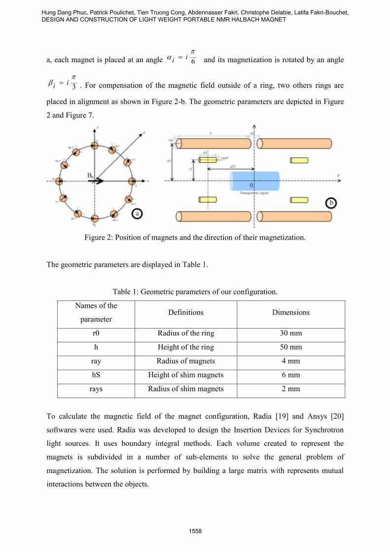
a, each magnet is placed at an angle 6ii

and its magnetization is rotated by an angle

3ii

. For compensation of the magnetic field outside of a ring, two others rings are

placed in alignment as shown in Figure 2-b. The geometric parameters are depicted in Figure

2 and Figure 7.

Figure 2: Position of magnets and the direction of their magnetization.

The geometric parameters are displayed in Table 1.

Table 1: Geometric parameters of our configuration.

Names of the

parameter Definitions Dimensions

r0 Radius of the ring 30 mm

h Height of the ring 50 mm

ray Radius of magnets 4 mm

hS Height of shim magnets 6 mm

rays Radius of shim magnets 2 mm

To calculate the magnetic field of the magnet configuration, Radia [19] and Ansys [20]

softwares were used. Radia was developed to design the Insertion Devices for Synchrotron

light sources. It uses boundary integral methods. Each volume created to represent the

magnets is subdivided in a number of sub-elements to solve the general problem of

magnetization. The solution is performed by building a large matrix with represents mutual

interactions between the objects.


1558

Ansys is a multiphysics software using FEM modeling. Each volume is divided with sub-

elements. Even the air between and around the magnets has to be meshed. The flux conditions

have to be placed outside the global volume in order to apply parallel or normal condition.

Usually, boundary integral method is considered faster than FEM. In our case, these two

complementary methods are implemented: Radia allowing a faster simulation, is used for

optimization and Ansys is used for verification and validation of results. The size of the

meshing is reduced until the simulation results do not change.

The properties of the material modeled magnets during simulation were chosen to represent

magnets from “HKCM MAGNETS from STOCK” [21]. The magnet material is Neodymium

NdFeB with the following characteristics:

a saturation magnetization of 1.37 T,

a coercivity Hc = 1000 kA/m,

the diameter and the length of the magnets are respectively 8 mm and 50 mm,

the maximal operating temperature is 120 °C,

the temperature coefficient is 0.11 %.°C-1

,

and the magnetization is oriented along the diameter.

In order to calculate the homogeneity, the values for the magnetic field are selected in the

homogeneous region and treated by Matlab Software. The homogeneity is calculated by the

formula (1).

6

10n i

i

Abs B B

BHomogeneitym

(1)

Where,

Bi is the value of magnetic field at the ith

position in the homogeneous region,

B is the magnetic field value at the center of the homogeneous region,

m is the number of mesh nodes in the homogeneous region.

III. SIMULATION RESULTS

a. Optimization of the gap between two rings without shim results

Our NMR portable magnet model is constituted with 24 magnets, placed as displayed in

Figure 7 and used for the simulations with Ansys and Radia. Considering the magnetic field

B0 oriented along Ox axis and the gap between two rings esp = 0, the maximum value of B0


1559

calculated with Radia is about of 0.103 T and of 0.11 T obtained with Ansys Analysis. The

difference of calculation between Radia and Ansys is about 6.79 %. This difference can be

accounted for by the problem of mesh size convergence. It means that the results obtained

with fine meshes are higher than those obtained with coarse meshes. Furthermore, the

difference is acceptable.

Figure 3-a represents the variation of the magnetic field B0 along the Ox axis. The value of

the magnetic field is almost constant for 1.8mm < x < 4.2mm. Figure 3-b represents the

variation of the magnetic field B0 in the plane xOy. Each shades of color represent a variation

of 50 ppm of the inhomogeneity 0

0

B

B

. In a rectangle of 5 6.4 mm

2, the inhomogeneity 0

0

B

B

is larger than 450 ppm (Radia) and 380 ppm (Ansys). For an inhomogeneity lower than 100

ppm, the expected volume for experiment is 3 3 3 mm3.

0 0.01 0.02 0.03 0.04 0.05 0.060.1

0.15

0.2

0.25

0.3

0.35

0.4

0.45

0.5

Distance (m)

Ma

gn

etic F

ield

(T

)

Magnetic Field simulation performed by Ansys

(a) Variation of magnetic field Bx versus x. (b) Inhomogeneity of the magnetic field Bx

versus x and y.

Figure 3: Magnetic Field Bx distribution at z = 0 (xOy plane).

The variation of the magnetic field Bx on the xOz plane is shown in Figure 4. The magnetic

field homogeneity in a region of 5 x 6.4 mm² is about 300 ppm determined by Radia, while

Ansys gives a result of 200 ppm.


1560

(a) Ansys Result. (b) Radia Result.

Figure 4: Magnetic Field Bx distribution in the region of 5 x 6.4 mm² in xOz plane.

The variation of profile of the magnetic field Bx along Oz axis depends on the esp gap

between the two rings. To optimize this gap, we increased the value of esp by steps of 0.1mm.

Figure 5 shows Bx profile for four values of esp. When esp = 0, the magnetic field outside

one ring does not compensate exactly the one of the other ring. For esp = 0.9 mm, the

compensation is optimum and the magnetic field at the center is almost constant.

0 0.005 0.01 0.015 0.02 0.025 0.03 0.035 0.04 0.045 0.050.102

0.103

0.104

0.105

0.106

0.107

0.108

0.109

0.11

0.111

0.112

Distance (m)

Ma

gn

etic F

ield

(T

)


0 0.01 0.02 0.03 0.04 0.05 0.060.101

0.102

0.103

0.104

0.105

0.106

0.107

0.108

0.109

Distance (m)

Ma

gn

etic F

ield

(T

)


(a) esp = 0 mm. (b) esp = 0.5 mm.


1561

0 0.01 0.02 0.03 0.04 0.05 0.060.101

0.102

0.103

0.104

0.105

0.106

0.107

0.108

Distance (m)

Ma

gn

etic F

ield

(T

)


0 0.01 0.02 0.03 0.04 0.05 0.060.101

0.102

0.103

0.104

0.105

0.106

0.107

Distance (m)

Ma

gn

etic F

ield

(T

)


(c) esp = 0.9 mm. (d) esp = 1.3 mm.

Figure 5: The field profile for different values of the gap esp between the two rings.

The “useful” volume for NMR sample is determined from the coordinates (x,y,z) of the point

where Bx is maximal. Then, the volume is calculated with the coordinates (x,y,z) that

generate a variation of 0

0

B

B

not higher than 100 ppm. The Figure 6 shows that the volume of

the homogeneous region is a function of the esp. The optimal value of esp determined by

Radia is around 0.77 mm and the “useful” volume is about 2640 mm3. When the spacing esp

between the two rings is optimized, the “useful” volume is increased by a ratio of around 80.

This is caused by the decrease of the magnetic field outside one ring, which is similar to the

increase of the other ring. There’s an optimum gap between the two rings where the sum of

the variations of the magnetic field outside the rings are canceled.

0 0.2 0.4 0.6 0.8 1 1.2 1.4 1.6 1.8 20

500

1000

1500

2000

2500

3000Value of the useful volume determined by Radia Simulation

Space between the two rings

Volu

me

Figure 6: Volume (mm3) for a variation of 0

0

B

B

lower than 100 ppm is a function of the gap

esp.


1562

b. Optimization of the configuration with shim magnets

Although the magnetic field homogeneity increases by adjusting the gap esp between the two

rings, the inhomogeneity of magnetic field also comes from magnetic material (dispersion of

both the value and the orientation of the magnetization), from errors in fabrication process and

positioning of the array magnets. These factors cannot be corrected only by adjustment of esp.

To overcome these difficulties, the shim magnets are considered as a way to compensate for

the inhomogeneity of the magnetic field [16][17][18]. In our case, we use eight small magnets

placed inside the bore of the two rings as shown in the Figure 7.

(a) With Ansys. (b) With Radia.

Figure 7: Halbach configuration with 24 magnets and 8 shim magnets, modeled with Ansys

and Radia.

The direction of magnetization of the shim magnets is defined as shown in Figure 8.


1563

Figure 8: Direction of magnetization of the 8 shim magnets.

There are three variables that need to be optimized: esp, r1 and dH. The optimization

objective is to determine the values for esp, r1 and dH that maximize the volume for an

inhomogeneity of 100 ppm. The flow chart shown in Figure 9 describes the optimization

process implemented with Mathematica software and the calculation of the magnetic field

with Radia software. To avoid the superposition of the main magnets and the shim magnets,

we set the range of r1 from 15 to 23 mm and the one for esp ranging from 0.1 to 0.6 mm. The

optimal value for esp, considered here, is different from the value considered before because

of the presence of shim magnets.

Each step of increase of r1 is 1 mm while correspondent value of esp is 0.1 mm. Each

possible values of r1 is placed in a matrix. The corresponding magnetic field and then the

three coordinates (x,y,z) for an homogeneity lower than 100 ppm are also determined. For

each value of r1, we have a value for the homogeneous volume. The value of r1 leading to the

highest value of the volume will be saved. The same process is repeated with the others

parameters esp and dH. After a variation of one parameter, the variation is refined around the

best value previously obtained. It’s very important to choose good initial conditions and

started the variation of one parameter with reliable value for the others parameters. This

method was preferred to the use of Mathematica software optimization functions, as

FindMaximum.


1564

Figure 9: Flow chart of our configuration with 24 main magnets and 8 shim magnets.

The optimized parameters are presented in the Table 2.

Table 2: The geometric parameters of an optimal configuration.

Name of the parameter Dimension

esp 0.2 mm

r1 20 mm

dH 26 mm

The optimizations results allow a great improvement of homogeneity, as it can be seen in

Figure 10. It shows that the inhomogeneity of the magnetic field calculated in a 7 x 8 mm²

region is 90 ppm after shimming while the value before shimming was 370 ppm.


1565

The magnetic field inhomogeneity calculated by Radia and by Ansys are in good agreement.

However, Ansys gives always smaller useful volumes than those obtained by Radia due to the

method of calculation. This can be explained by the fact that Radia result is the highest value

at the region edge while Ansys compute the mean value for the overall region.

(a) Before shimming. (b) After shimming.

Figure 10: Magnetic field homogeneity in the xOy plane and z = 0.

The Figure 11 shows great improvement of homogeneity along Oz axis. The size of the

homogeneous region increases drastically in length from 8 mm to 20 mm. This is confirmed

by the stability of the magnetic field profile of the Figure 12.


Figure 11: Magnetic field homogeneity in the region 8 x 20 mm2 along Oz axis


1566

0 0.005 0.01 0.015 0.02 0.025 0.03 0.035 0.04 0.045 0.050.102

0.103

0.104

0.105

0.106

0.107

0.108

0.109

0.11

0.111

0.112

Distance (m)

Ma

gn

etic F

ield

(T

)


0 0.01 0.02 0.03 0.04 0.05 0.060.106

0.1065

0.107

0.1075

0.108

0.1085

0.109

0.1095

0.11

0.1105

Distance (m)

Ma

gn

etic F

ield

(T

)



Figure 12: Magnetic field profiles at the center of our Halbach arrangement of magnets.

As shown in Figure 13, the inhomogeneity of magnetic field in a volume of 7 x 8 x 20 mm3

are respectively 4320 ppm without shim magnets and of 230 ppm with the shim magnets.


Figure 13: Magnetic field distribution in the 3D sensitive volume: 7 x 8 x 20 mm3.

IV. PROTOTYPE DESIGN AND EXPERIMENTAL SET UP

a. Prototype design

The prototype consists of two rings of 12 magnets each one. These magnets are placed on a

circle of 30 mm radius and inserted into the twelve holes of two aluminum frames. The two

rings of the prototype, fixed by some screws on the aluminum frames, can slide on three rods,

to achieve the desired position. The highest value of the magnetic field magnets measured at

the center of the frame, allow us to determine their rotation angles and to fix them by the

dedicated screws as shown on Figure 14.


1567

(a) Shim magnets that can move along three degrees of

freedom.

(b) Halbach prototype with the slide-blocks used to

move the shim magnets in radial direction.

Figure 14: Picture of the prototype with shim magnets.

Each shim magnet shown on the Figure 14 is glued in a nonmagnetic cylinder. These

cylinders can rotate, move along the longitudinal axis and slide along the radius of the

prototype to find the optimal position of the shim magnets. These cylinders are placed in the

holes of sliding-blocks moving on the four apertures of an aluminum frame concentric with

the prototype.

b. Experimental setup

The magnetic field is measured by the digital gaussmeter Hirst GM08 with sensitivity limit of

10-4

T in the range 0 – 0.299 T. The micropositioner Signatone S-926 is used to control the

probe movement in three directions as shown in the Figure 15. The resolution is 254 µm per

knob revolution. Matlab software carries out the plotting of the measurable values.


1568

Figure 15: Measurement set-up of the magnetic field in the prototype.

V. EXPERIMENTAL RESULTS

a. Measurements before shimming

To optimize the gap esp between two rings, at the beginning, it was set at 0 mm, and was

progressively increased by turning the screws on the frame of the device (Figure 15).

The Figure 16 shows the magnetic field profiles in Oz direction for four different gaps esp

between the rings. The optimal gap is displayed in Figure 16-c where the magnetic strength is

equal to 0.138 T and remains constant for the distance of 10 mm. The shapes of the curves

plotted in the Figure 16 are similar to those obtained by simulation in the Figure 5.

0 10 20 30 40 50 600.124

0.126

0.128

0.13

0.132

0.134

0.136

0.138

0.14

Distance (mm)

Ma

gn

etic F

ield

(T

)

Magnetic Field Measurement

0 10 20 30 40 50 60

0.128

0.13

0.132

0.134

0.136

0.138

0.14

Distance (mm)

Ma

gn

etic F

ield

(T

)


(a) esp = 0. (b) esp = 1.6 mm.

The three screws

used to adjust the

gap esp between

two rings

The probe

Signatone S-926

Hirst

GM08


1569

0 10 20 30 40 50 600.131

0.132

0.133

0.134

0.135

0.136

0.137

0.138

0.139

Distance (mm)

Ma

gn

etic F

ield

(T

)


0 5 10 15 20 25 30 35 40 45 50

0.125

0.126

0.127

0.128

0.129

0.13

0.131

0.132

0.133

0.134

Distance (mm)

Ma

gn

etic F

ield

(T

)


(c) esp = 2.4 mm. (d) esp = 6.4 mm.

Figure 16: Magnetic field profiles in Oz direction for different esp values.

The magnetic field distribution shown in Figure 17, is measured at z = 0, in the region 6 x 6.5

mm² (xOy). In this region, the homogeneity value is respectively 1399 ppm calculated by

formula (1) and 380 ppm obtained by simulation. It means that the measurable homogeneity

is approximately 3.5 times worse than that simulated (Figure 3-b).

Figure 17: The magnetic field distribution in xOy plane obtained by measurement before

shimming.

Figure 18 shows the magnetic field distribution measurement in xOz plane in the region of 7 x

20 mm². In this region the homogeneity calculated by formula (1) is equal to 1426 ppm. This

homogeneity is of 4415 ppm in the volume of 6 x 7 x 20 mm3.

The magnetic field distribution is similar to the simulation as shown in the Figure 4.

0 1 2 3 4 5 60

1

2

3

4

5

6

7

X (mm)

The field distribution measured in XOY plane ( before shimming )

Y (

mm

)

0.136

0.1361

0.1362

0.1363

0.1364

0.1365

0.1366

0.1367

0.1368

0.1369

0.137


1570

-3

-2

-1

0

1

2

3

-10-8-6-4-20246810

The measured magnetic field distribution in xOz plane before shimming

Z (mm)

X (

mm

)

0.1353

0.1354

0.1355

0.1356

0.1357

0.1358

0.1359

0.136

0.1361

0.1362

0.1363

Figure 18: The measured magnetic field distribution in xOz plane before shimming.

b. Measurements after shimming

Figure 19 shows the improvement of the magnetic field homogeneity in xOy plane in the

same region 6 x 6.5 mm². The homogeneity is respectively, 1399 ppm before shimming

calculated by formula (1) and 817 ppm after shimming.


Figure 19: Magnetic field homogeneity at z = 0 in xOy plane.

In the region of 7 x 20 mm2

(xOz plane), the homogeneity calculated by formula (1) is 894

ppm while it is 1426 ppm without shim magnets. The magnetic field homogeneity with shim

magnets shows in Figure 20, achieved in the volume 6 x 7 x 20 mm3 is 1335 ppm in

comparison to 4415 ppm obtained without shim magnets. The magnetic field homogeneity is

3.3 times better. Figure 20 shows the improvement of the homogeneity that is approximate

0 1 2 3 4 5 60

1

2

3

4

5

6

7

X (mm)


Y (

mm

)

0.136

0.1361

0.1362

0.1363

0.1364

0.1365

0.1366

0.1367

0.1368

0.1369

0.137

0 1 2 3 4 5 60

1

2

3

4

5

6

7

X (mm)

The field distribution measured in XOY plane ( after shimming )

Y (

mm

)

0.1369

0.137

0.1371

0.1372

0.1373

0.1374

0.1375

0.1376


1571

5.8 times worse than the simulated value. The measured and simulated field distribution in

xOz plane are similar as shown in the Figure 4.

-3

-2

-1

0

1

2

3

-10 -8 -6 -4 -2 0 2 4 6 8 10

The measured magnetic field distribution in xOz plane after shimming

Z (mm)

X (

mm

)

0.1357

0.1358

0.1359

0.136

0.1361

0.1362

0.1363

Figure 20: The magnetic field homogeneity in xOz plane after shimming.

VI. DISCUSSION

The difference between the simulated and measured values of the magnetic field homogeneity

is due to the poor quality of the magnets. There is a large dispersion of the magnets properties.

For our prototype we selected 24 magnets among 27 having a similar magnetic field strength

and the magnets 5, 22 and 23 was rejected. This was done with the measurement of the

magnetic field on each tip of the magnet cylinder. Table 3 shows the value of B1 and B2 for 27

magnets and the misalignment angle α. B1 and B2 are respectively the magnetic field in the

vicinity of the two faces of the magnet cylinder as shown on the


1572

Figure 21. The average value of the magnetic field is around 27.3 mT. The misalignment

angle represents the error of orientation of the radial direction of the magnetic field on each

face. In ideal case, this angle value is zero but for some magnets this value can reach 17

degrees and the consequence, is an error of homogeneity of the magnetic field.

Table 3: Magnetic field and misalignment angle measured on each tip of the 27 magnets.

Magnet 1 2 3 4 5 6 7 8 9 10

B1 (mT) 27.3 27.2 27.3 27.2 27.3 27.2 27.1 27.0 26.9 27.0

B2 (mT) 27.2 27.1 27.5 27.1 27.0 27.1 27.2 26.9 27.0 27.2

(degree) 0 0 8 9 17 8 0 0 0 12

Magnet 11 12 13 14 15 16 17 18 19 20

B1 (mT) 27.4 27.2 27.2 27.2 27.3 27.3 27.3 27.4 27.4 27.4

B2 (mT) 27.5 27.0 27.2 27.4 27.4 27.3 27.5 27.4 27.5 27.2

(degree) 0 10 0 12 0 0 12 0 0 8

Magnet 21 22 23 24 25 26 27

B1 (mT) 27.3 27.2 27.6 27.3 27.4 27.4 27.3

B2 (mT) 27.3 27.5 27.5 27.4 27.3 27.5 27.4

(degree) 0 16 4 6 9 7 8

(a) Magnet cylinder with B1 and B2 the

magnetic field in the vicinity of its two

faces and the misalignment angle α.

(b) Picture of Magnet cylinder.


1573

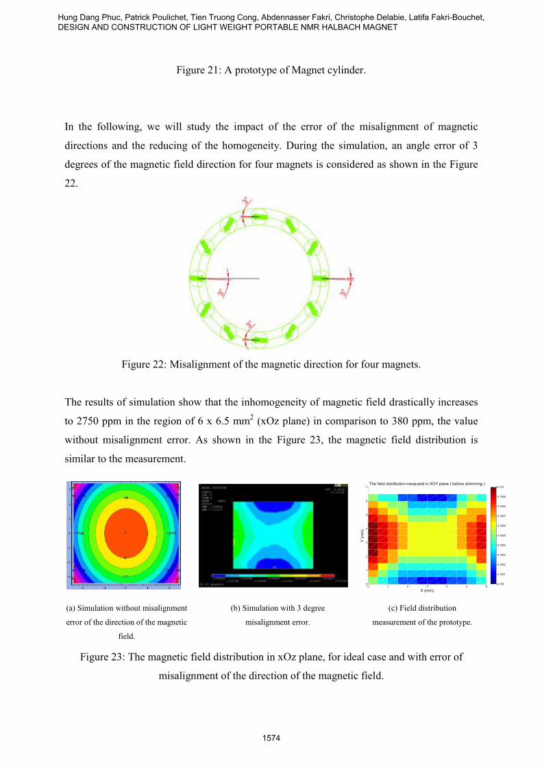
Figure 21: A prototype of Magnet cylinder.

In the following, we will study the impact of the error of the misalignment of magnetic

directions and the reducing of the homogeneity. During the simulation, an angle error of 3

degrees of the magnetic field direction for four magnets is considered as shown in the Figure

22.

Figure 22: Misalignment of the magnetic direction for four magnets.

The results of simulation show that the inhomogeneity of magnetic field drastically increases

to 2750 ppm in the region of 6 x 6.5 mm2 (xOz plane) in comparison to 380 ppm, the value

without misalignment error. As shown in the Figure 23, the magnetic field distribution is

similar to the measurement.

(a) Simulation without misalignment

error of the direction of the magnetic

field.

(b) Simulation with 3 degree

misalignment error.

(c) Field distribution

measurement of the prototype.

Figure 23: The magnetic field distribution in xOz plane, for ideal case and with error of

misalignment of the direction of the magnetic field.

0 1 2 3 4 5 60

1

2

3

4

5

6

7

X (mm)


Y (

mm

)

0.136

0.1361

0.1362

0.1363

0.1364

0.1365

0.1366

0.1367

0.1368

0.1369

0.137


1574

VII. CONCLUSION

The study presented here depicts two methods of simulation and the main measurement

results of a light weight NMR portable Halbach type magnet. We described the optimization

process of this permanent magnet designed with two rings of 12 magnets each one, that

provide a magnetic field B0 around 0.1 T. The simulation results have been published in [22].

The study describes the used based on the Radia software process, for calculate and simulate

the magnetic field B0 and its homogeneity. We verified also those results with the finite

element software Ansys multiphysics. The obtained results with the two softwares are in good

agreement. Based on the software analysis, we simulated the homogeneity of magnetic field

and optimized the gap esp of the two consecutive rings to increase the size of the

homogeneous region. The optimum gap length is around esp= 0.8 mm. The measurement of

the magnetic field profile for different values of the gap esp between the two rings give a

similar value of the optimal gap.

To compensate for the magnetic field inhomogeneity caused by the errors of fabrication

process and the dispersion of the magnetic properties of the magnets, we used eight small

shim magnets placed at the center of the device. By optimizing their position, the

homogeneity had been significantly improved. The results of optimization shows that the

homogeneity for a given volume (7 x 8 x 20 mm3) is improved 18 times in comparison to the

same configuration without shim magnets. Thus the value of the homogeneity decrease from

4320 ppm to 230 ppm.

For a given volume of 6 x 7 x 20 mm3, the measurement of the magnetic field variation,

shows the same homogeneity improvement, using the shim magnets. Thus the homogeneity is

of 1335 ppm while it was of 4415 ppm for the case without shim magnets. The magnetic field

homogeneity was enhanced of a 3.3 factor. However, there is still a difference between the

simulation and the measurement, which could be explained by the poor quality of the

magnets. For each used magnets for the NMR device design, the magnetic field on the tip of

the cylindrical magnet and the misalignment angle of the radial magnetic field were


1575

measured. The misalignment angle could be as high as 17 degrees. The simulations with some

misalignment angle error of 3 degree on four magnets were performed and the same shape of

the magnetic field distribution was obtained. Thus we attribute the difference between the

simulation and the measurement to the misalignment angle of the magnets.

Despite these results, there’s a good agreement between the simulation results and the

measurement.

REFERENCES

[1] S. Anferova, V. Anferov, M. Adams, P. Blümler, N. Routley, K. Hailu, K.

Kupferschläger, M. j. d. Mallett, G. Schroeder, S. Sharma, and B. Blümich, “Construction

of a NMR-MOUSE with short dead time,” Concepts Magn. Reson., vol. 15, no. 1, pp. 15–

25, Mar. 2002.

[2] G. Moresi and R. Magin, “Miniature permanent magnet for table-top NMR,” Concepts

Magn. Reson., vol. 19B, no. 1, pp. 35–43, 2003.

[3] G. Navon, U. Eliav, D. E. Demco, and B. Blümich, “Study of order and dynamic

processes in tendon by NMR and MRI,” J. Magn. Reson. Imaging, vol. 25, no. 2, pp.

362–380, Feb. 2007.

[4] F. J. Rühli, T. Böni, J. Perlo, F. Casanova, M. Baias, E. Egarter, and B. Blümich, “Non-

invasive spatial tissue discrimination in ancient mummies and bones in situ by portable

nuclear magnetic resonance,” J. Cult. Herit., vol. 8, no. 3, pp. 257–263, Jul. 2007.

[5] B. Blümich, F. Casanova, J. Perlo, S. Anferova, V. Anferov, K. Kremer, N. Goga, K.

Kupferschläger, and M. Adams, “Advances of unilateral mobile NMR in nondestructive

materials testing,” Magn. Reson. Imaging, vol. 23, no. 2, pp. 197–201, Feb. 2005.

[6] T. Poli, L. Toniolo, M. Valentini, G. Bizzaro, R. Melzi, F. Tedoldi, and G. Cannazza, “A

portable NMR device for the evaluation of water presence in building materials,” J. Cult.

Herit., vol. 8, no. 2, pp. 134–140, Apr. 2007.

[7] H. Pedersen, S. Ablett, D. Martin, M. J. Mallett, and S. Engelsen, “Application of the

NMR-MOUSE to food emulsions,” J. Magn. Reson., vol. 165, no. 1, pp. 49–58, Nov.

2003.

[8] B. Blümich, V. Anferov, S. Anferova, M. Klein, R. Fechete, M. Adams, and F. Casanova,

“Simple NMR-mouse with a bar magnet,” Concepts Magn. Reson., vol. 15, no. 4, pp.

255–261, Dec. 2002.


1576

[9] W.-H. Chang, J.-H. Chen, and L.-P. Hwang, “Single-sided mobile NMR with a Halbach

magnet,” Magn. Reson. Imaging, vol. 24, no. 8, pp. 1095–1102, Oct. 2006.

[10] C. W. Windt, H. Soltner, D. van Dusschoten, and P. Blümler, “A portable Halbach

magnet that can be opened and closed without force: The NMR-CUFF,” J. Magn. Reson.,

vol. 208, no. 1, pp. 27–33, Jan. 2011.

[11] X. Zhang, V. Mahesh, D. Ng, R. Hubbard, A. Ailiani, B. O’Hare, A. Benesi, and A.

Webb, “Design, construction and NMR testing of a 1 tesla Halbach Permanent Magnet for

Magnetic Resonance,” in COMSOL Users Conference, Boston, 2005.

[12] K. Halbach, “Design of permanent multipole magnets with oriented rare earth cobalt

material,” Nucl. Instrum. Methods, vol. 169, no. 1, pp. 1–10, Feb. 1980.

[13] H. Raich and P. Blümler, “Design and construction of a dipolar Halbach array with a

homogeneous field from identical bar magnets: NMR Mandhalas,” Concepts Magn.

Reson. Part B Magn. Reson. Eng., vol. 23B, no. 1, pp. 16–25, Oct. 2004.

[14] H. Soltner and P. Blümler, “Dipolar Halbach magnet stacks made from identically

shaped permanent magnets for magnetic resonance,” Concepts Magn. Reson. Part A, vol.

36A, no. 4, pp. 211–222, Jul. 2010.

[15] B. P. Hills, K. M. Wright, and D. G. Gillies, “A low-field, low-cost Halbach magnet

array for open-access NMR,” J. Magn. Reson., vol. 175, no. 2, pp. 336–339, Aug. 2005.

[16] E. Danieli, J. Mauler, J. Perlo, B. Blümich, and F. Casanova, “Mobile sensor for high

resolution NMR spectroscopy and imaging,” J. Magn. Reson., vol. 198, no. 1, pp. 80–87,

May 2009.

[17] C. Hugon, F. D’Amico, G. Aubert, and D. Sakellariou, “Design of arbitrarily

homogeneous permanent magnet systems for NMR and MRI: Theory and experimental

developments of a simple portable magnet,” J. Magn. Reson., vol. 205, no. 1, pp. 75–85,

Jul. 2010.

[18] R. C. Jachmann, D. R. Trease, L.-S. Bouchard, D. Sakellariou, R. W. Martin, R. D.

Schlueter, T. F. Budinger, and A. Pines, “Multipole shimming of permanent magnets

using harmonic corrector rings,” Rev. Sci. Instrum., vol. 78, no. 3, p. 035115, Mar. 2007.

[19] "Radia Introduction." [Online].

http://www.esrf.eu/Accelerators/Groups/InsertionDevices/Software/Radia/Documentation/Intr

oduction. [Accessed: 05-Oct-2014].

[20] “ANSYS - Simulation Driven Product Development.” [Online]. Available:

http://www.ansys.com/. [Accessed: 13-Aug-2014].


1577

[21] “HKCM MAGNETS from STOCK, from FACTORY & MAGNETS ON DEMAND.”

[Online]. Available: https://www.hkcm.de/expert.php. [Accessed: 11-Jul-2014].

[22] P. Poulichet, Hung Dang Phuc, Tien Truong Cong, Latifa Fakri-Bouchet, Abdennasser

Fakri, and Christophe Delabie, “Simulation and optimisation of homogeneous permanent

magnet for portable NMR applications,” 8th International Conference on Sensing

Technology, Liverpool, UK., 04-Sep-2014.


1578

design and construction of light weight portable …

Documents