design and characterization of an altitude chamber …
TRANSCRIPT

DESIGN AND CHARACTERIZATION OF AN ALTITUDE CHAMBER
FOR CHEMICAL ROCKET ENGINES
by
Jacob M. McCormick
A Thesis
Submitted to the Faculty of Purdue University
In Partial Fulfillment of the Requirements for the degree of
Master of Science in Aeronautics and Astronautics
School of Aeronautics & Astronautics
West Lafayette, Indiana
August 2019

2
THE PURDUE UNIVERSITY GRADUATE SCHOOL
STATEMENT OF COMMITTEE APPROVAL
Dr. Timothée Pourpoint, Chair
Department of Aeronautics and Astronautics
Dr. Stephen Heister
Department of Aeronautics and Astronautics
Dr. William Anderson
Department of Aeronautics and Astronautics
Approved by:
Dr. Wayne Chen
Head of the Graduate Program

3
Dedicated to my friends and loved ones. You’ve stood by me, even in the hardest of times. It is
now my turn to do the same for you.

4
ACKNOWLEDGMENTS
I owe my success in graduate school to a great multitude of people. Dr. Pourpoint has
played an essential role in my development as an aerospace engineer. He is the ideal
representation of a mentor and advisor, and he has laid the foundation for my success both in
academia and industry. I want to thank Scott Meyer for the constructive criticism provided for
various project designs implemented over the last two years. I’d also like to thank Rob and Toby
for providing input regarding various designs. Through your design suggestions and critiques,
the path from theoretical model to physical component has become slightly smoother.
I also want to thank Ben Whitehead for acting as a sounding board for different thesis
ideas and always being willing to answer, “even the silly questions.” While not necessarily
directly influential on my thesis, each member of Dr. Pourpoint’s lab has made a lasting impact.
Thank you everyone for making the last two years memorable in the form of different projects:
developing the altitude chamber, preparing the atmospheric JPL tests, creating the MON
synthesis stand, etc. Each of these experiences has helped to shape me into the aerospace
engineer that I am today.

5
TABLE OF CONTENTS
LIST OF TABLES .......................................................................................................................... 6
LIST OF FIGURES ........................................................................................................................ 7
NOMENCLATURE ..................................................................................................................... 10
ABSTRACT .................................................................................................................................. 12
1. INTRODUCTION ................................................................................................................. 14
2. EJECTOR BACKGROUND ................................................................................................. 16
3. EJECTOR MODELING BACKGROUND ........................................................................... 27
4. MODELING DEVELOPMENT AND RESULTS ............................................................... 35
Huang Model: Overview................................................................................................... 35
Huang Model: Sensitivity Analysis Results ..................................................................... 38
Huang Model: Single-Stage Ejector Characterization Results ......................................... 49
New Model: Overview ...................................................................................................... 58
New Model: Single-Stage Ejector Characterization Results ............................................ 62
New Model: Single-Stage Ejector Solid Rocket Motor Test Results ............................... 64
New Model: Two-Stage Ejector Characterization Results ............................................... 68
New Model: Two-Stage Ejector 90 Newton Rocket Engine Test Results ....................... 72
Graphical User Interface: Overview ................................................................................. 74
5. JPL MOTOR DESIGN .......................................................................................................... 77
Injector Assembly Design ................................................................................................. 80
Main Pipe Section/Partial Design ..................................................................................... 85
Nozzle Assembly Design .................................................................................................. 87
Nozzle Assembly Thermal Analysis ................................................................................. 89
Finite Element Analysis (FEA) ......................................................................................... 95
6. CONCLUSIONS ................................................................................................................... 97
7. FUTURE WORK................................................................................................................... 99
APPENDIX A. MATLAB CODES ............................................................................................ 104
APPENDIX B. MACHINE DRAWINGS .................................................................................. 163
REFERENCES ........................................................................................................................... 101

6
LIST OF TABLES
Table 1: Geometrical dimensions of the motive nozzles used for experimental performance
characterization [26]. ........................................................................................................ 31
Table 2: Geometrical dimensions of the constant-area sections for experimental performance
characterization [26]. ........................................................................................................ 32
Table 3: Fluid characteristics for argon, steam, and air. ............................................................... 47
Table 4: Test cases evaluated to determine bounds for suction fluid parameters. ........................ 47
Table 5: Relevant dimensions of single-stage ejector. .................................................................. 50
Table 6: Table displaying all relevant dimensions for the three nozzles. ..................................... 51
Table 7: Specifications for Aerotech F-50 solid rocket motor [32]. ............................................. 65
Table 8: Relevant values for the two-stage ejector system. .......................................................... 69
Table 9: Relevant flow conditions for the rocket engine test using the two-stage ejector. .......... 72

7
LIST OF FIGURES
Figure 1: Representation of major components of a single-stage ejector [6]. .............................. 16
Figure 2: Relationship between ejector performance and back pressure (discharge pressure) [8].
........................................................................................................................................... 18
Figure 3: Two-stage ejector system configured in series with example static pressure and mass
flow rate distribution. ........................................................................................................ 19
Figure 4: Two-stage ejector system configured in parallel with example static pressure and mass
flow rate distribution. ........................................................................................................ 21
Figure 5: Geometry of a constant-area ejector [15]. ..................................................................... 22
Figure 6: Motive plume flow lines for different motive nozzle exit pressures [10]. .................... 24
Figure 7: Control volume approach with consideration for area change and mixing [19]. .......... 27
Figure 8: Graphical representation of the calculation architecture for the 1-D model proposed by
Huang et al. [26]. .............................................................................................................. 30
Figure 9: Velocity distribution of shock circle model compared to traditional 1-D model [27]. . 33
Figure 10: Impact of motive stagnation temperature on single-stage ejector performance. ......... 39
Figure 11: Impact of suction stagnation temperature on single-stage ejector performance. ........ 41
Figure 12: Results showing impact of motive molecular weight on single-stage ejector
performance. ..................................................................................................................... 42
Figure 13: Results showing impact of suction molecular weight on single-stage ejector
performance. ..................................................................................................................... 43
Figure 14: Results showing impact of motive heat capacity ratio on single-stage ejector
performance. ..................................................................................................................... 44
Figure 15: Results showing impact of suction heat capacity ratio on single-stage ejector
performance. ..................................................................................................................... 45
Figure 16: Sensitivity graph showing the influence of 10% changes to the input parameters. .... 46
Figure 17: Sensitivity graph showing the influence of input parameters over real-world operating
ranges. ............................................................................................................................... 48
Figure 18: Sensitivity graph showing the response of simulated altitude to each input parameter.
........................................................................................................................................... 49
Figure 19: CAD rendering of single-stage ejector. ....................................................................... 50

8
Figure 20: P&ID describing the experimental configuration for the performance characterization
of the single-stage ejector. ................................................................................................ 52
Figure 21: Results from the first experimental testing campaign for single-stage ejector with
original motive nozzle....................................................................................................... 53
Figure 22: Graph of experimental results for 8.5 expansion ratio nozzle. .................................... 54
Figure 23: Graph of experimental results for 4.67 expansion ratio nozzle. .................................. 54
Figure 24: Flow chart describing model analysis architecture for Huang Model. ........................ 55
Figure 25: Graph showing satisfactory suction coefficient values for motive pressure and suction
mass flow range of single-stage ejector. ........................................................................... 56
Figure 26: Graph showing satisfactory motive plume coefficient values for motive pressure and
suction mass flow range of single-stage ejector. .............................................................. 56
Figure 27: Graph showing satisfactory mixing coefficient values for motive pressure and suction
mass flow range of single-stage ejector. ........................................................................... 57
Figure 28: Flow chart describing analysis procedure for new model. .......................................... 62
Figure 29: Graph of the momentum coefficient versus motive stagnation pressure and suction
mass flow for original nozzle. ........................................................................................... 62
Figure 30: Graph relating the momentum coefficient, motive stagnation pressure, and suction
mass flow for the 8.5 expansion ratio nozzle. ................................................................... 63
Figure 31: Graph relating the momentum coefficient, motive stagnation pressure, and suction
mass flow for the 4.67 expansion ratio nozzle. ................................................................. 64
Figure 32: Graph of the thrust profile for the Aerotech F50-9T solid rocket motor [32]. ............ 65
Figure 33: Relationship between exhaust mass flow and suction stagnation pressure. ................ 66
Figure 34: Graph showing overlay of equivalent nitrogen flow for F50-9T motor on performance
characterization graph with original nozzle. ..................................................................... 67
Figure 35: Flow chart displaying procedure for using characterization data and equivalent
nitrogen flow treatment to extend model prediction capabilities. ..................................... 68
Figure 36: CAD rendering of the two-stage ejector system. ........................................................ 69
Figure 37: Relationship between 1st stage suction stagnation pressure and 1st stage suction mass
flow rate for two-stage ejector system. ............................................................................. 70
Figure 38: Graph showing momentum coefficient versus suction mass flow rate for first stage
ejector. .............................................................................................................................. 71

9
Figure 39: Graph showing momentum coefficient versus suction mass flow rate for second stage
ejector. ............................................................................................................................... 71
Figure 40: Comparison on momentum coefficient value between characterization data and
equivalent nitrogen flow for rocket engine test for 1st stage ejector. ................................ 73
Figure 41: Comparison on momentum coefficient value between characterization data and
equivalent nitrogen flow for rocket engine test for 2nd stage ejector. ............................... 73
Figure 42: Screen of model GUI used to specify the number of ejector stages used. .................. 74
Figure 43: Screen of model GUI used to specify 1st stage suction flow values. ........................... 75
Figure 44: Screen of model GUI used to specify 1st stage motive flow values. ........................... 75
Figure 45: Screen of model GUI used to specify 2nd stage motive flow values. .......................... 76
Figure 46: CAD model cutaway view showing all major design components of injector housing,
as well as the full-cone spray injector. .............................................................................. 81
Figure 47: CAD model depicting full injector assembly. ............................................................. 82
Figure 48: CAD cutaway view showing instrumentation ports in the injector flange used for
combustion chamber pressure and temperature measurement.......................................... 83
Figure 49: CAD cutaway view showing the normal and shortened motor configurations. .......... 86
Figure 50: CAD cutaway view showing the major design elements associated with the overall
nozzle assembly. ............................................................................................................... 88
Figure 51: COMSOL thermal analysis result for 2 and 5 second firing durations without TBC. 90
Figure 52: Thicknesses and locations of TBC application. .......................................................... 91
Figure 53: Thermal analysis results for 2 and 5 second firing durations with TBC. .................... 92
Figure 54: Graph of the extrusion limits for different material O-rings [37]. .............................. 93
Figure 55: Minimum thermal expansion of nozzle housing/expansion section after 2 and 5
second firing duration. ...................................................................................................... 94
Figure 56: Maximum thermal expansion of nozzle insert after 2 and 5 second firing duration. .. 94
Figure 57: Relationship between 316 SS yield strength and temperature in Kelvin [38]. ............ 95
Figure 58: Final CAD rendering for the new JPL motor. ............................................................. 96

10
NOMENCLATURE
𝐴 - Area (m2)
𝐴𝑡 - Bolt cross sectional area (m2)
𝐶𝑑 - Discharge coefficient
𝐶𝑝 - Specific heat (J/kg-K)
D - Diameter (m)
𝐸𝑅 - Expansion ratio
𝛾 - Heat capacity ratio
�� - Mass flow rate (kg/s)
𝑀 - Mach number
𝑀𝑊 - Molecular weight (kg/mol)
𝑁 - Number of items
𝜂𝑚 - Momentum coefficient
𝜂𝑝 - Motive nozzle efficiency
𝜂𝑠 - Suction efficiency
𝑁𝑢𝐷 - Nusselt number
𝑂/𝐹 - Mixture Ratio
P - Pressure (Pa)
𝜙𝑝 - Motive plume efficiency
𝜙𝑚 - Mixing efficiency
Pr - Prandtl number
𝑅 - Specific Gas Constant (J/kg-K)
Re - Reynold’s number
𝑅𝑢 - Universal gas constant (J/mol-K)
𝜌 - Density (kg/m3)
𝜎 - Stress (Pa)
𝑇 - Temperature (K)
𝑉 - Velocity (m/s)
~𝑡 - Motive nozzle throat value

11
~0 - Stagnation Value
~𝑚𝑖𝑥 - Mixed flow value
~𝑁2 - Equivalent nitrogen value
~𝑜𝑝𝑡 - Optimum value
~𝑝 - General motive value
~𝑝0 - Motive Stagnation Value
~𝑝1 - Motive nozzle exit value
~𝑝2 - Motive pre-contraction value
~𝑝3 - Motive value after normal shock
~𝑝𝑦 - Motive value at hypothetical throat
~𝑠 - General suction value
~𝑠0 - Suction Stagnation Value
~𝑠2 - Suction pre-contraction value
~𝑠𝑦 - Suction value at hypothetical throat
~3 - Value after normal shock in constant area section

12
ABSTRACT
Author: McCormick, Jacob, M. MS
Institution: Purdue University
Degree Received: August 2019
Title: Design and Characterization of an Altitude Chamber for Chemical Rocket Engines.
Committee Chair: Dr. Timothée Pourpoint
Over the course of a launch, a rocket experiences a broad range of atmospheric pressures,
influencing the performance of the rocket nozzle. Aside from implementing a complex system
to modulate the geometry of the rocket nozzle, it is nearly impossible to optimize the overall
performance of the rocket engine for the entirety of the burn. It is therefore necessary for
engineers to optimize the performance for a specific atmospheric pressure range. For this reason,
facilities exist which are capable of testing propulsion systems at relevant operational conditions.
This is accomplished by simulating the atmospheric pressure relevant to the altitude of interest in
a closed volume, also known as an altitude chamber.
This thesis focuses on the development of reduced pressure testing capabilities at Zucrow
Laboratories. A two-stage ejector on loan from NASA Marshall is used in series with a
supersonic diffuser to allow for the testing of up to100 lbf rocket engines at equivalent altitudes
of up to 100,000 ft. The objective of this research is to implement a one-dimensional (1-D)
model which accurately predicts the performance of the two-stage ejector in real time, informing
the maximum thrust and simulated altitude capabilities within the altitude chamber located in
room 134A of ZL3 during experimental testing.
A new 1-D model was created which efficiently balances computational performance
with prediction accuracy. The new model was validated using experimental data collected for a
smaller single-stage ejector utilizing facility nitrogen as the suction fluid and facility air as the
motive fluid. The validated model was then shown to accurately predict the performance of the
single-stage ejector system during the testing of a small solid rocket motor (SRM) within the
altitude chamber. The new 1-D model was then calibrated using experimental data from the two-
stage ejector on loan from NASA Marshall. It was shown that the new model is capable of
predicting the performance of the two-stage ejector for varying rocket engine configurations. As

13
a result, this new model was proven to be a viable predictive tool to inform the testing
capabilities of the altitude facility at Zucrow Labs.
In addition, a new rocket engine is designed for the characterization of a hybrid grain
configuration within the altitude chamber at reduced pressure, which serves as a continuation of
the atmospheric testing campaign performed in collaboration with the Jet Propulsion Laboratory
(JPL).

14
1 INTRODUCTION
Prior to a space launch, it is often necessary to characterize the performance of the
vehicle’s engines at relevant atmospheric pressure conditions. For example, the performance of
a high expansion ratio rocket nozzle designed to operate in the vacuum of space cannot be
validated at sea level conditions. It is therefore necessary to simulate the ambient pressure
conditions relevant to the altitude of interest for the mission. This is commonly accomplished
using a closed vessel (often called an altitude chamber), in addition to a device capable of
maintaining the reduced pressure environment within the chamber. There are a few different
methods to achieve this steady reduced pressure, including vacuum pumps, ejectors, and
supersonic diffusers. While each of these three devices is discussed below, only the ejector
system will be discussed in sections to follow.
As the leak rate associated with pumps is dictated primarily by how well the dynamic
seals can prevent entrained gases from escaping, these devices are capable of reaching extremely
low pressures. This makes pumps ideal for testing rocket engines in extremely low pressure
environments. However, pumps are constant volumetric flow devices, removing a set volume of
gases per revolution. For this reason, testing higher thrust motors requires a proportionate or
even exponential increase in the scale of the pump employed. This is because all of the internal
components of the pump must scale to meet the increased demand on the overall system. For
this reason, testing rocket engines with high thrust levels is often difficult using a pump alone.
Supersonic diffusers avoid this limitation by converting the kinetic energy of exhausted
gases back into pressure. The recovery of pressure within a supersonic diffuser is accomplished
through a complex system of shocks that occur within the second throat. Supersonic diffusers
are capable of a maximum theoretical compression ratio, which limits the minimum pressure that
can be maintained within the altitude chamber, assuming that the supersonic diffuser is
exhausting to ambient pressure (14.7 psia). While it has been shown in the literature that
supersonic diffusers are capable of performing reduced pressure testing unassisted [1], achieving
extremely low pressures within the altitude chamber requires the use of subsequent vacuum
systems to reduce the back pressure immediately downstream of the supersonic diffuser exit.
Ejectors and supersonic diffusers are commonly used concurrently to achieve reduced
pressure conditions relevant to the testing of high-expansion ratio rocket engines for space

15
applications. The ejector system acts to reduce the back pressure experienced by the supersonic
diffuser, allowing for the combined system to maintain a pressure much lower than the
supersonic diffuser alone. Similar to supersonic diffusers, ejectors convert the kinetic energy of
a motive fluid (air in our case) into pressure using a complex system of shocks within the
constant area section of the ejector. Both ejectors and supersonic diffusers are capable of
handling exhaust flow rates much higher than a pump of comparable scale.
In the same way that a single-stage ejector coupled with a supersonic diffuser increases
the overall compression ratio of the system, multiple ejectors can be placed in series to achieve a
comparable increase in pressure recovery capabilities. Employing a multi-stage ejector
configuration has been shown to yield a significant improvement in overall system performance
and efficiency when compared with a single-stage ejector of similar size [2]. The altitude facility
in ZL3 at Zucrow Laboratories employs a two-stage ejector coupled with a supersonic diffuser to
maintain a simulated altitude of up to 100,000 ft during the testing of rocket engines up to
100 lbf.
As each engine characterized using the altitude facility applies different loads to the
vacuum system, it is beneficial to predict the motive flow conditions necessary to support a given
testing campaign. This expedites the process of testing while simultaneously conserving facility
air. This a-priori determination of necessary testing conditions is accomplished through
modeling. While there are multiple modeling schemes which can be implemented to accomplish
this performance prediction, one-dimensional models are by far the most computationally
efficient. This modeling class can predict the performance of the vacuum system in real time,
making it a viable tool to be used in an experimental testing environment. A comprehensive
literature review was performed to determine the viability of existing models, and it was
determined that a new 1-D model was necessary to meet the needs of the altitude facility at ZL3.
In this thesis, a new quasi one-dimensional model was developed to accurately predict the
performance of the two-stage ejector system over the full operational range of pressures and thrust
values achievable by the new altitude facility in ZL3 at Zucrow Laboratories. This thesis also
summarizes the design of a new hybrid rocket engine, which will rely on the predictive capabilities
of the new model to determine the maximum achievable simulated altitude for experimental testing
within the altitude chamber.
16
2 EJECTOR BACKGROUND
Ejectors have been employed since 1901 [3], with applications ranging from
refrigeration systems and powder transportation to jet thrust augmentation and the
characterization of rocket motors for space operation [4]. This wide-spread application of
ejectors is largely due to the robust nature of ejector operation. Ejectors are simple in design and
have no moving parts, thus minimizing operational cost and maintenance frequency [5]. A
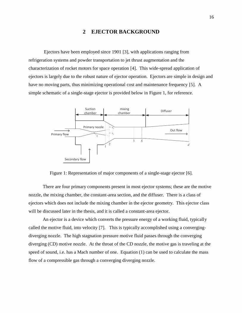
simple schematic of a single-stage ejector is provided below in Figure 1, for reference.
Figure 1: Representation of major components of a single-stage ejector [6].
There are four primary components present in most ejector systems; these are the motive
nozzle, the mixing chamber, the constant-area section, and the diffuser. There is a class of
ejectors which does not include the mixing chamber in the ejector geometry. This ejector class
will be discussed later in the thesis, and it is called a constant-area ejector.
An ejector is a device which converts the pressure energy of a working fluid, typically
called the motive fluid, into velocity [7]. This is typically accomplished using a converging-
diverging nozzle. The high stagnation pressure motive fluid passes through the converging
diverging (CD) motive nozzle. At the throat of the CD nozzle, the motive gas is traveling at the
speed of sound, i.e. has a Mach number of one. Equation (1) can be used to calculate the mass
flow of a compressible gas through a converging diverging nozzle.

17
mp =Pp,0At
√Tp,0√γp
Rp(
2
γp + 1)
(γp+1)/(γp−1)
(1)
The motive flow then expands isentropically to a Mach number above one in the
diverging section of the motive nozzle. Equation (2) can be used to determine the isentropic
relationship between the Mach number and the static pressure of a flow.
P
P0= (1 +
γ − 1
2M2)
−γγ−1
(2)
As the motive gas exits the converging-diverging nozzle, it continues to accelerate
isentropically in the mixing chamber until a pressure is reached which is at, or below, the static
pressure of the suction fluid. The suction fluid is the gas that is to be evacuated from the altitude
chamber in the case of motor performance characterization at reduced pressures. For the
majority of operating cases, the Mach number of the suction flow at the ejector inlet is
sufficiently low to assume stagnation conditions. This produces a favorable pressure gradient
between the motive and suction fluids, causing the suction fluid to be entrained into the mixing
chamber [8]. It is a combination of this pressure gradient, and momentum transfer from the
motive flow to the suction flow through shear, which induces mixing between the supersonic
motive flow and subsonic suction flow within the mixing chamber.
The two fluids continue mixing through the converging section between the mixing
chamber and the constant-area section of the ejector. Momentum is transferred from the motive
flow to the suction flow, resulting in a supersonic mixed flow. The constant-area section length
is chosen to ensure that the two fluids are properly mixed well before the entrance to the diffuser
section of the ejector [9]. At some point within the constant-area section of the ejector, a normal
shock occurs which irreversibly converts the kinetic energy of the mixed flow into pressure. The
static pressure of the subsonic mixed flow following the normal shock can be determined using
gas dynamic relations. The subsonic mixed flow then expands in the diffuser section of the
ejector, reaching approximately stagnation conditions. This is the final stage of pressure

18
recovery within the ejector, and the subsonic mixed flow is then either exhausted to the
atmosphere or fed into the next ejector stage in the system.
In order to ensure optimal ejector operation, the ejector must recover the static pressure
of the suction fluid to the ambient pressure conditions present at the exit plane of the ejector-
diffuser. The ambient pressure at the exit plane of the diffuser section is known as back
pressure. If the static pressure of the mixed flow at the exit plane of the diffuser is less than the
back pressure, there exists an adverse pressure gradient back into the diffuser [10]. This adverse
pressure gradient acts to move the shock wave present in the constant-area section of the ejector
further upstream. As the normal shock moves further upstream, the effective mixing length for
the motive and suction flow is reduced. This decrease in mixing length reduces mixing
efficiency, negatively impacting overall ejector performance. Once the back pressure rises to a
critical level, the shock structure moves out of the constant-area section and into the mixing
chamber of the ejector [11]. At this back pressure level, the effective compression ratio of the
ejector is drastically reduced [12]. This results in a steep rise in altitude chamber pressure, given
constant motive/suction flow conditions. The back pressure at which ejector performance begins
to deteriorate is called the critical back pressure. A graph showing the relationship between
ejector performance and back pressure is given in Figure 2 below.
Figure 2: Relationship between ejector performance and back pressure (discharge pressure) [8].

19
For a single-stage ejector exhausting to the atmosphere, the back pressure is held constant
at 14.7 psia. However, for a multiple-stage ejector, the back pressure that an ejector stage
experiences can vary. For a multiple-stage ejector system configured in series, the exit of the
upstream ejector is connected to the suction inlet of the downstream ejector. An example of this
configuration is given in Figure 3 for reference, which shows a typical static pressure and mass
flow rate distribution for two ejectors connected in a series configuration.
Figure 3: Two-stage ejector system configured in series with example static pressure and mass
flow rate distribution.
Figure 3 shows that the back pressure experienced by the first stage ejector is dependent
on the compression ratio of the second stage. For this discussion, it is important to understand
that the back pressure for the second-stage ejector is a constant value of 14.7 psia. If the
compression ratio of the second stage ejector is compromised, the suction inlet pressure of the
second-stage ejector (back pressure of the first-stage ejector) increases accordingly. As the
0.6 lbm/s
1.9 lbm/s
14.7 psia
0.1 lbm/s
2 psia
400 psia
10 psia 0.7 lbm/s
1.2 lbm/s
400 psia
REDUCED
PRESSURE
VESSEL
1st Stage
Ejector
2nd Stage
Ejector

20
compression ratio across the first-stage ejector remains constant, the static pressure within the
altitude chamber must increase.
In the same way, if the compression ratio of the first-stage ejector is compromised, the
exit pressure of the first-stage (suction inlet of the second-stage) decreases. As the second-stage
compression ratio remains constant, the exit pressure of the second-stage ejector also decreases.
The back pressure for the second-stage ejector has not changed (still 14.7 psia), and thus there
exists an adverse pressure gradient back into the second-stage ejector-diffuser. The normal
shock in the constant-area section of the second-stage ejector then moves upstream into the
mixing chamber. This breaks the performance of the second-stage ejector, as discussed earlier,
further decreasing the overall compression ratio of the two-stage ejector system. Ultimately, this
interaction again leads to a sharp rise in altitude chamber static pressure. In this way, it can be
seen that the performance of each ejector in a two-stage ejector system configured in series is
highly dependent on the other.
Another characteristic of a series configuration ejector system is that, for a constant
geometry and motive conditions, the downstream ejector has a lower compression ratio
capability than that of the upstream ejector. Figure 3 shows that the mixed flow exiting the first-
stage ejector is handled as the suction flow of the second-stage ejector. The downstream ejector
stage must be designed to handle both the original suction flow being evacuated from the altitude
chamber and the motive flow of the upstream ejector stage. This results in a lower compression
ratio capability, as the compression efficiency of ejectors decreases with increased suction load.
It is common to use a slightly larger downstream ejector stage to handle the increased suction
load [13]. This example illustrates the general behavior of a multiple-stage ejector configured in
series. Multiple-stage ejector systems can also be configured in parallel with one another. An
example of this configuration is given in Figure 4, which shows a typical pressure and mass flow
rate distribution for a two-stage ejector configured in parallel.

21
Figure 4: Two-stage ejector system configured in parallel with example static pressure and mass
flow rate distribution.
The same two ejectors are used in this example as in the series configuration to isolate
only the effect of changing the configuration of the ejector system. In Figure 4, the static
pressure within the altitude chamber is much higher than for the series configuration. However,
the suction mass flow rate is much higher for the parallel configuration when compared with the
series configuration.
There are a few conclusions that can be made based on these results. Multiple-stage
ejector systems configured in series are typically capable of higher overall compression ratios.
However, the series configuration is generally more sensitive to changes in operating conditions
for all stages of the ejector system. Multiple-stage ejector systems configured in parallel benefit
from a higher relative suction mass flow rate capability, but do not have the benefit of a multiple-
stage combined compression ratio. For this reason, multiple-stage ejectors configured in series
400 psia
0.5 lbm/s
8 psia
0.2 lbm/s 0.6 lbm/s
400 psia
1.2 lbm/s
8 psia
0.7 lbm/s
0.8 lbm/s
14.7 psia
14.7 psia
1.7 lbm/s
REDUCED
PRESSURE
VESSEL
1st Stage
Ejector
2nd Stage
Ejector

22
are generally more practical when high vacuum levels are desired. A multiple-stage ejector
system configured in parallel is more appropriate when the system must handle relatively large
suction mass flow rates. For example, a multiple-stage ejector system configured in series would
be appropriate for the testing of a low thrust rocket motor at high vacuum levels, while a
multiple-stage ejector system configured in parallel would be more appropriate for the testing of
a high thrust rocket motor at pressures closer to sea level conditions (14.7 psia).
While there are significant performance benefits to be had employing ejector systems,
they do suffer from relatively low energy efficiencies when compared to alternative compression
devices [5]. This is due to the normal and oblique shocks occurring at the exit of the ejector
nozzle and within the constant area section of the ejector, as well as high frictional and shear
losses. The inherent inefficiency associated with ejectors is compensated by the fact that ejectors
rely on a high stagnation pressure motive gas as their energy source. As many facilities in
industry produce steam as a result of relevant production processes [14], it is common for
ejectors supporting these processes to utilize steam as their motive source. Zucrow Laboratories
has a large volume of high pressure air that is used to support a multitude of experimental tests,
and thus it is more practical to use high pressure air as the motive source for the two-stage
ejector system in the altitude facility.
While ejectors can vary in scale from millimeters to feet, they can generally be divided
into two main groups based on their geometry. There are two main types of ejectors – constant-
area ejectors and constant-pressure ejectors - each of which induce mixing between the motive
and suction fluids in different ways. A constant area ejector is the simpler of the two ejector
geometries and can be seen in Figure 5 below.
Figure 5: Geometry of a constant-area ejector [15].

23
The motive nozzle of a constant-area ejector is slightly extended, with the motive gas
leaving the exit plane of the converging diverging nozzle in the constant area section of the
ejector. In this way, the “mixing chamber” only serves to hold the stagnant suction gas before it
is entrained by the motive fluid in the constant area section of the ejector. The mixing of the
motive and suction fluids occurs only in the constant-area section of a constant-area ejector. The
mixing process associated with a constant-area ejector is greatly simplified, as there is no change
in area over the mixing length; this can again be seen in Figure 5. This geometric simplification
can make the process of modeling significantly easier, as there is no area change to account for.
However, it has been shown in literature that a constant-area ejector is less efficient than a
constant-pressure ejector of comparable size [16]. The main difference between a constant-area
and constant-pressure ejector is the location of the motive nozzle exit plane. The motive nozzle
exit plane is located near the middle of the mixing chamber for a constant-pressure ejector. The
altitude facility at Zucrow Laboratories uses a two-stage constant-pressure ejector system. For
this reason, the remainder of this thesis will focus only on modeling the performance of a
constant-pressure ejector.
Constant-pressure ejectors allow for constant-pressure mixing between the motive and
suction flows. The overall geometry of a constant-pressure ejector can be seen in Figure 1. As
stated earlier, the exit plane of the motive nozzle is located approximately in the middle of the
mixing chamber for a constant-pressure ejector. While there have been multiple experimental
and theoretical studies which have focused on determining the optimum location for the exit
plane of the motive nozzle in a constant-pressure ejector, this is an adequate generalization for
the discussion. Entrainment begins close to the exit of the CD nozzle, with the two flows
interacting through the contraction region of the mixing chamber and into the constant-area
section of the ejector. The mixing processes occurring in the constant-area section and diffuser
are unchanged between the two types of ejectors. These two types only influence the mixing of
the two fluids leading into the constant-area section.
Ejectors can also be classified based on the motive and suction fluids that are being used
in the ejector system. There are three main classes of ejectors: liquid-liquid, liquid-gas, and gas-
gas ejectors [17]. Liquid-liquid ejectors depend on the incompressible interaction of the two
fluid flows to perform the compression within the ejector. Liquid-gas ejectors are the most
complex of the three ejector classes from a modeling perspective. This ejector class requires the

24
model to handle two-phase flow interactions at supersonic velocities. The gas-gas ejector class
is most applicable to this thesis and requires the modeling of compressible flow interactions
between the suction and motive fluids. As gas-gas ejector modeling is most applicable to the
two-stage ejector system at Zucrow Laboratories, this thesis will focus on this ejector class and
exclude the other two classes.
An ejector is designed from the factory to operate most efficiently at a single point on its
operating curve [18]. The majority of the initial experimental validation for this model was
performed using a small-single stage ejector, which was optimized from the factory to perform
most efficiently at a motive pressure of 215 psia. Decreasing the motive pressure below 215 psia
decreases the performance of the ejector. This makes sense intuitively, as one would expect that
decreasing the energy throughput of the device would decrease the performance of the ejector
system. It was found during the experimental characterization of the single-stage ejector that
increasing the motive pressure beyond 215 psia also decreases the performance of the ejector.
This may be a surprising result, as the theoretical energy available to the ejector system increases
with higher motive pressures. However, this is an accepted result in industrial ejector design,
and the CFD results in literature help to explain this phenomenon. The theoretical results of a
paper written in 2009 by Kumaran et al. are given in Figure 6 below.
Figure 6: Motive plume flow lines for different motive nozzle exit pressures [10].

25
These theoretical results from CFD modeling can help us better understand the
interaction mechanisms occurring within the ejector during nominal and off-design operation.
The discussion below is informed by the results of Kumaran et al. [10]. As can be seen from the
equation for mass flow across a converging-diverging nozzle, as well as the isentropic relation
between stagnation and static pressure, the static pressure at the exit plane of the converging-
diverging nozzle increases with increasing upstream stagnation pressure. It can also be seen
from the equation for mass flow across a converging-diverging nozzle that increasing mass flow
requires a proportionate increase in upstream stagnation pressure. Section b) of Figure 6 shows
the operation of the ejector at its optimized motive stagnation pressure value. In this section, the
motive plume expands just to the wall of the constant-area section of the ejector. The
momentum losses within the ejector are minimized, and there is no reversed flow of gases back
into the mixing chamber of the ejector.
The mass flow specified in section a) of Figure 6 requires a lower motive stagnation
pressure than section b), and thus yields a lower static pressure at the exit plane of the motive
nozzle. Because the static pressure at the exit plane of the nozzle is lower for section a) than for
section b), the motive plume doesn’t fully expand to fill the constant-area section of the ejector.
It can be seen in section a) of Figure 6 that there are recirculation regions between the motive
plume and the wall of the ejector. These recirculation regions further reduce the momentum of
the motive jet plume and allow for leak paths from the atmosphere back into the mixing chamber
of the ejector. These factors ultimately result in an altitude chamber static pressure that is higher
than optimal.
The mass flow in section c) of Figure 6 requires a higher stagnation pressure than
section b), resulting in a higher motive static pressure at the exit plane of the motive nozzle. The
motive gas at the exit plane of the nozzle is under-expanded for section c) when compare to that
of section b), and thus results in greater expansion of the motive plume downstream. The motive
plume then impacts the converging section of the ejector, dissipating large amounts of
momentum and energy [10]. This loss of momentum and energy reduces the efficiency of the
ejector at the operation conditions given in section c), again decreasing the performance of the
ejector. In this discussion, it can be seen that there are multiple factors which lead to sub-
optimal performance for off-design motive stagnation pressures within an ejector.

26
It is important to understand the fundamental interactions that determine the performance
of an ejector. By understanding each of the driving interactions within an ejector, it is possible
for the designer to create a model which more accurately predicts the overall performance of the
ejector system. Failing to understand these interactions can lead to incorrect assumptions which
do not accurately capture ejector system performance. Often, within a model, it is more
beneficial not to make assumptions until the physical behavior of the system is fully understood.
Having provided a brief description of the operation of a single and multiple-stage ejector
system, it is now appropriate to discuss the various models that have been presented in literature
over the years.

27
3 EJECTOR MODELING BACKGROUND
The interaction between the two fluids within the mixing chamber of the ejector is
perhaps the least understood aspect of ejector operation. This interaction region within the
ejector is a driving motivator for the wide array of models that exist in the literature. There are a
few different theoretical methods which can be used to predict the performance of an ejector
system; each of these methods varies in computational time, complexity, and accuracy.
Computational Fluid Dynamics (CFD) is by far the most accurate method for modeling
ejector performance. However, CFD is computationally expensive and sensitive to input
conditions. It is often necessary to perform an initial validation for a given mesh before
extending that simulation structure to unsolved problems. CFD is generally more appropriate
when a deep understanding of the flow interactions is necessary, and it has become a popular
modeling approach within academia as the computational power of computers has increased.
CFD can also be used to inform more simplistic one dimensional models, allowing the developer
to understand the overarching flow processes that are otherwise difficult to determine
experimentally.
The next class of methods are one-dimensional (1-D) models. One-dimensional models
often adopt a control volume approach, where relevant flow values are calculated at discrete
points within the ejector. An example of a control volume calculation methodology is given in
Figure 7.
Figure 7: Control volume approach with consideration for area change and mixing [19].
28
There are three main classes of 1-D modeling methods: empirical, semi-empirical
(hybrid), and purely theoretical methods. Empirical models are the simplest type of model, with
no underlying equations being developed to define the performance of the ejector system.
Instead, this model type is fully informed by experiment, with regression analysis being
performed to develop fits for the experimental data. While empirical models are useful for
quickly interpolating between data points over the ejector’s operating range, this model class
cannot be used to make predictions for different ejector geometries or even fluid types [20]. For
this reason, empirical models are only useful for characterizing the performance of an ejector
system with non-variable geometry and flow conditions. Empirical models are useful in
traditional industrial processes, where an ejector system may have essentially constant operating
conditions, with only small changes in suction load or motive supply pressure.
Semi-empirical models, or hybrid models, contribute a set of flow equations which define
the general processes occurring within an ejector. Many of the more complex fluid interactions –
turbulent mixing, shock structures, wall friction – are absorbed into a hybrid model using
corrective coefficients which are introduced throughout the model’s calculation architecture.
These types of models benefit from a greater potential for extension when compared with purely
empirical models, but still cannot accurately define all fluid interactions that occur during
nominal ejector operation. With this model class, it is possible to predict the performance of an
ejector with slight variations in ejector geometry and flow conditions. These performance
prediction capabilities make this model class popular in industries that handle varying fluid types
and operating temperatures/pressures. This model is also not computationally expensive, with
flow solutions being determined in a short amount of time relative to purely theoretical models.
The most complex one-dimensional model class is that of the purely theoretical model.
Purely theoretical models do not rely on experimental data to inform the modeling process.
Similar to CFD, purely theoretical models only rely on experimental data for initial validation.
Once validated, purely theoretical models can be extended to a vast array of ejector geometries
and operating conditions. This large prediction benefit of purely theoretical models over the two
previously mentioned modeling classes is balanced by a large increase in both computational
time and model complexity. In this sense, purely theoretical models are similar to CFD in
implementation. Purely theoretical models are therefore inappropriate for real-time predictions

29
of ejector performance [21]. This model class is instead more commonly used in academia, or
when the performance of an ejector cannot be determined based on prior experimental results.
Each of the three model classes stated above has certain benefits and drawbacks. It is the
job of the developer to determine which of these classes best suits the modeling needs of his/her
project. A short overview of the various relevant models introduced in literature is given below.
For this historical summary, only semi-empirical models are discussed. It was determined that
the semi-empirical modeling class achieved a good balance between computational efficiency
and model accuracy.
There have been many different models introduced in the literature over a nearly century-
long period of sustained research effort. Each of these models makes slightly different
assumptions and introduces novel calculation methodologies for the prediction of ejector
performance. The first known mathematical model for predicting the performance of ejectors
was introduced in 1942 by Keenan and Neumann [22]. This model calculated the performance
of a single-stage constant area-ejector using ideal gas dynamics, as well as conservation of mass,
energy, and momentum. Compressible gas dynamics, as well as the fundamental conservation
laws, has been used in a majority of subsequent models. In 1950, the concept of constant-
pressure mixing was introduced by Keenan et al. [23], stating that the static pressures of the
motive and suction flows were equal downstream of the exit plane of the motive nozzle. The
motive and suction flows then mixed at equal/constant pressure through the converging section
and into the constant-area section of the ejector.
While much theoretical work was being performed to better understand the function of
ejectors, there were parallel experimental studies which sought to visually determine the
interaction of the motive and suction fluids as they travel through the ejector. In the late 1950’s
and early 1960’s, this visualization was commonly achieved using a method called vapor
screening, where vapors are introduced into the motive flow upstream of the nozzle. These
vapors then condense in the mixing section, and act as tracer particles for visualization of the
flow [24]. The results of these visual studies better informed theoretical models, further
improving their physical accuracy. Variants of these early visualization techniques are used
today, and they continue to provide valuable insights regarding the complex processes occurring
in the ejector during mixing.

30
The results of experimental visualization by Fabri and Siestrunck [25] helped to inform a
new model which defined a fictive suction throat located upstream of the constant-area section of
the ejector [12]. At some point upstream of the constant-area section of the ejector, it is assumed
that the suction flow reaches sonic velocity. It is also assumed that mixing between the two
flows only occurred downstream of this fictive suction throat. It is important to mention this
assumption present in this model, as many models proposed in subsequent publications make
similar assumptions with slight variations.
One of the more popular models, which is cited throughout the literature recently, is the
one-dimensional model proposed by Huang et al. in 1999 [26]. This model is developed to
predict the performance of a constant-pressure mixing ejector, and makes the assumption of a
fictive suction throat originally presented by Munday and Bagster [12]. While there are many
simplifying assumptions made in this model, perhaps the most significant is the assumption that
the suction throat is located at the entrance to the constant-area section of the ejector. This
assumption can be seen graphically in Figure 8.
Figure 8: Graphical representation of the calculation architecture for the 1-D model proposed by
Huang et al. [26].
The cross section y-y is denoted as the location of the suction throat; it is assumed that the
two flows only mix downstream of the suction throat. This assumption simplifies the
calculations necessary to simulate the mixing of the two fluids, as there is no area change that
occurs during this mixing process. However, it does not accommodate mixing between the exit
plane of the motive nozzle and the constant-area section of the ejector. This semi-empirical

31
model also relies on four corrective coefficients which must be informed using experimental
results. These four corrective coefficients are introduced to account for motive nozzle, motive
plume, suction acceleration, and mixing losses. When fitting more than one corrective
coefficient to experimental data, it is essential that there exist orthogonal results. This means
that a given experimental operating condition for an ejector cannot be satisfied by two different
combinations of corrective coefficients. If there is more than one combination of corrective
coefficient values which satisfies a given operating point, then any of the successful
combinations can be chosen when fitting the model to the experimental data. When fitting the
model to experimental data, it is necessary to have smooth curves which relate the value of the
corrective coefficient to the data. Smooth corrective coefficient curve fits allow for interpolation
between points on the operating curve of the ejector. As the number of corrective coefficients
increases, the number of potential inter-relations between corrective coefficients also increases.
The 1-D model proposed by Huang et al. was experimentally validated using small
ejectors with different nozzle geometries and constant-area section diameters. The geometrical
dimensions for the ejector configurations used in the experimental validation process are given in
Table 1 and Table 2.
Table 1: Geometrical dimensions of the motive nozzles used for experimental performance
characterization [26].
Nozzle Throat Diameter (mm) Exit Diameter (mm) Expansion Ratio
A 2.64 4.5 2.905
E 2.82 5.1 3.27

32
Table 2: Geometrical dimensions of the constant-area sections for experimental performance
characterization [26].
Constant-area Section Diameter (mm) Inlet Converging Angle (°)
A 6.7 68
B 6.98 60
C 7.6 67
D 8.1 68
E 8.54 67
F 8.84 67
G 7.34 60
H 9.2 62
Experimental data was collected by Huang et al. for different combinations of these
nozzle and constant-area section geometries. Using the experimental data collected, the author
made conclusions regarding the four corrective coefficients defined within the model.
Many publications are presented in literature which either build upon the model
architecture of Huang et al., or use the experimental results to validate their own model. One of
the more recent one-dimensional models presented in literature is the shock circle model,
published in 2007 [27]. This model introduces a velocity distribution for the two fluid flows. In
prior models, a uniform velocity was assigned to each of the two fluids, with no consideration for
radial variation in fluid velocity. Figure 9 shows the shock circle model velocity distribution
compared to the traditional discrete velocity treatment of prior one-dimensional models.

33
Figure 9: Velocity distribution of shock circle model compared to traditional 1-D model [27].
The shock circle model provides a slightly more realistic treatment of the two fluids by
satisfying the no-slip boundary condition on the walls of the ejector [27]. It is once again
assumed that the suction throat is located at the entrance to the constant-area section of the
ejector. The developed model is then validated using the experimental data present in the
publication by Huang et al.
In 2010, the comprehensive ejector model was introduced in literature by Liao and Best
[19]. The comprehensive ejector model is a purely theoretical model which uses a multiple
control volume approach, along with the conservation laws, to simulate the mixing of the motive
and suction fluids from the exit plane of the motive nozzle to the exit of the diffuser [19]. There
are no corrective coefficients present in this model, and thus the model relies on experimental
data only for validation rather than model fitting. While the comprehensive ejector model
benefits from an extension in predictive capabilities due to the purely theoretical treatment of
ejector performance, the model also suffers from increased complexity and computational cost.
Other popular theoretical models in literature include the finite difference model [28],
delayed equilibrium model [29], homogeneous equilibrium model [30], and method of
characteristics [31]. Each of these models has powerful predictive capabilities. However, the
discussion of these models is outside the scope of this thesis. Purely theoretical models, as well
as purely empirical models, will be excluded from discussion for the remainder of the thesis.
The early stages of this thesis focus on adapting the model proposed by Huang et al. for use in
predicting the performance of the 2-stage ejector located in the altitude facility in ZL3 of Zucrow

34
Laboratories. It is determined that a simplified 1-D model is necessary to accurately predict the
performance of this two-stage ejector system at relevant test conditions. The model development
section of this thesis highlights the primary motivations surrounding the creation of a revised
one-dimensional model and describes the calculation architecture for this new model.

4 MODELING DEVELOPMENT AND RESULTS
It was necessary to quickly develop an effective model which could accurately predict the
performance of the large-scale two-stage ejector system at the altitude facility of Zucrow Labs.
If possible, a simple model existing in literature would be implemented. Using an existing
model would save on development time while still allowing for the accurate prediction of the
two-stage ejector system. The primary model used in the preliminary stages of this thesis was
contributed by Huang et al. [26]. For clarity, it is called the Huang Model within this thesis, as it
was primarily implemented in the first semester of this thesis. This model has been widely cited
in literature and is shown to produce good agreement with experimental results. This one-
dimensional model falls into the semi-empirical modeling class and achieves near real-time
ejector performance prediction capabilities while simultaneously maintaining sufficient
prediction accuracy. While this model was originally created to define the performance of a
single-stage ejector within a refrigeration system, we hoped that this model could be used with
similar success for a two-stage vacuum ejector system.
As work on this thesis continued to progress, it became clear that the one-dimensional
model proposed by Huang et al. was insufficient to properly predict the performance of the two-
ejector system at Zucrow Laboratories. The theoretical results which informed this conclusion
are given later in the thesis, along with a promising model which is potentially capable of
extending the prediction capabilities of existing semi-empirical models.
Huang Model: Overview
From the literature review on existing ejector models, it was initially determined that the
one-dimensional semi-empirical model proposed by Huang et al. was most appropriate for our
applications. This model relies only on input values defining flow characteristics at the motive
and suction inlets to the ejector system. This is a major benefit, as it is difficult to collect
experimental data regarding flow conditions within the mixing and constant area sections of the
ejector system without extensive design modifications. This input-based modeling architecture
simplifies the testing procedure for collecting data necessary to properly inform the one-
dimensional model. Furthermore, the calculation architecture for Huang et al.’s model is simple

relative to purely theoretical methodologies. Another advantage of a simple calculation
architecture is that the model is less sensitive to changes in relevant parameters. In theory, this
increased robustness requires less fine adjustment by the end user, making the model easier to
use and troubleshoot.
As the final results of this thesis are not based upon the semi-empirical model proposed
by Huang et al., the model’s architecture is not discussed in complete detail. However, the
assumptions in the model are given within this thesis, along with the equations relevant to the
conclusions drawn during model development. Many of the assumptions made by Huang et al.
are also used in the new model proposed within this thesis. The inclusion of the supporting
assumptions and equations will help to form a more complete understanding regarding the
motivations for creating a new model which is computationally more simplistic than that
proposed by Huang et al.
The list given below is taken directly from the publication by Huang et al. [26], and
summarizes all of the major assumptions that are made within the one-dimensional model.
1. The working (motive) fluid is an ideal gas with constant properties Cp and γ.
2. The flow inside the ejector is steady and one-dimensional.
3. The kinetic energy at the inlets of the motive and suction ports and the exit of diffuser are
negligible.
4. For simplicity in deriving the 1-D model, the isentropic relations are used as an
approximation. But to account for non-ideal processes, the effects of frictional and mixing
losses are considered by using coefficients introduced in the isentropic relations. These
coefficients are related to the isentropic efficiency and need to be determined experimentally.
5. After exhausting from the nozzle, the primary flow fans out without mixing with the
entrained flow until some cross section y–y (hypothetical throat) which is inside the constant-
area section.
6. The two streams start to mix at the cross section y–y (hypothetical throat) at uniform
pressure, i.e. Ppy = Psy, before the shock which is at the cross section s–s.
7. The entrained flow is choked at the cross section y–y (hypothetical throat).
8. The inner wall of the ejector is adiabatic.

Based on assumption 4 given in the list above, there are four corrective coefficients
which are introduced into the model’s calculation architecture. The first corrective coefficient,
ηp, is introduced into Equation (3) to account for non-isentropic losses in the motive converging-
diverging nozzle when calculating the mass flow of motive gases.
mp =Pp,0At
√Tp,0
√γp
Rp(
2
γp + 1)
(γp+1)(γp−1)
⁄
√ηp (3)
The second corrective coefficient in the model is introduced to account for losses in the
suction flow. The model proposed by Huang et al. assumes that the suction fluid reaches sonic
velocity at an annular throat in the entrance to the constant-area section of the ejector. As a
result, the mass flow of suction gases can be calculated in the same way that mass flow is
calculated through a converging-diverging nozzle. Equation (4) defines the mass flow of suction
gases for the ejector and is identical to the equation for mass flow through a converging-
diverging nozzle.
ms =Ps,0Asy
√Ts,0
√γsRs
(2
γs + 1)
(γs+1)(γs−1)
⁄
√ηs (4)
There is also a corrective coefficient which accounts for losses relevant to the expansion
of the motive plume leading into the constant area section of the ejector. As stated in
assumptions 5 and 6, the gases exiting the motive nozzle continue to expand isentropically until
the static pressure of the motive fluid is equivalent to the static pressure of the suction fluid at
sonic velocity. Equation (5) is used to calculate the final expanded area of the motive flow, and
it includes a corrective coefficient, ∅p, to account for these expansion losses.

Apy
Ap1=
∅pMpy
[2
γp + 1(1 +
γp − 12 Mpy
2)]
(γp+1)
(2(γp−1))⁄
1Mp1
[2
γp + 1(1 +
γp − 12 Mp1
2)]
(γp+1)
(2(γp−1))⁄
(5)
The final corrective coefficient, ∅𝑚, is defined to account for momentum losses within
the constant area section of the ejector during mixing between the motive and suction fluids.
Equation (6) utilizes conservation of momentum to determine the velocity of the mixed flow.
∅m(mpVpy + msVsy) = (mp + ms)Vm (6)
There are two constraints which are introduced in the Huang Model architecture. First,
the sum of the suction and motive flow areas must be equivalent to the flow area in the constant-
area section of the ejector. This is a geometrical constraint, and it is satisfied using the
appropriate combination of ∅𝑝 and 𝜂𝑠 values. Second, the static pressure at the exit plane of the
ejector-diffuser must be greater than or equal to the ambient pressure (14.7 psia for a single-stage
ejector). This constraint acts to account for the critical back pressure of the system. Different
combinations of these four corrective coefficients are inserted into the model. The combination
of coefficient values defined for a given experimental data point is that which satisfies the
constraints defined within the equation.
Huang Model: Sensitivity Analysis Results
The model proposed by Huang et al. was first used to determine the impact of different
motive and suction flow parameters on the performance of the single-stage ejector system. This
characterization step was important, as the two-stage ejector system would eventually handle
rocket exhaust products with varying static temperatures, heat capacities, and molecular weights.
As Huang et al. had already experimentally validated the one-dimensional model, it was assumed
that the modeling results could be used as a preliminary estimate of performance. For this

reason, some early conclusions were drawn from the modeling results before in-house validation
was completed.
It was determined experimentally by Huang et al. that the corrective coefficients were
relatively insensitive to changes in flow parameters [26]. For this reason, the coefficient values
defined experimentally by Huang et al. were used to determine the impact of different flow
parameters on the performance of the ejector system. This analysis varied eight input parameters
to determine the impact of different motive and suction flow characteristics on the performance
of the ejector system. The performance of the ejector system is defined to be the maximum
entrainment ratio for a given suction total pressure. The entrainment ratio is defined as the ratio
of suction mass flow to motive mass flow, and it helps to describe the overall efficiency of the
ejector. The entrainment ratio capability is defined for the full range of motive total pressures
that can be supplied to the single-stage ejector. The first flow parameter to be varied is motive
stagnation temperature, and the results of this analysis are given in Figure 10.
Figure 10: Impact of motive stagnation temperature on single-stage ejector performance.
As can be seen in Figure 10, increasing the stagnation temperature of the motive fluid
acts to increase the relative performance of the ejector system. This may seem counter-intuitive
initially, as an increase in motive stagnation temperature yields a decrease in motive mass flow

given otherwise constant flow conditions. However, the main mixing for this model is
determined using conservation of momentum. The increase in motive stagnation temperature
yields a proportional increase in motive mixing temperature. This higher mixing temperature
corresponds to a higher speed of sound, and thus higher momentum value for the motive fluid
during mixing. It is also important to note that decreasing the motive mass flow improves the
entrainment ratio, assuming that the entrainment capacity of the ejector system is otherwise
unchanged.
One behavior present in the graphs of Figure 10 through Figure 15 is a cutoff after some
minimum motive pressure. This cutoff is an artifact of the model’s calculation architecture. The
modeling background of this thesis mentions a critical back pressure at which the ejector
transitions from critical to sub-critical operation mode. In this model, it is assumed that the
suction flow fails to choke in the constant-area section of the ejector during sub-critical
operation. As the kinetic energy of the motive stream decreases, the pressure recovery capability
of the ejector also decreases. The cutoff point in the graphs signifies the motive pressure at
which the energy throughput of the motive flow is insufficient to sustain choking of both the
motive and suction flows. The next flow parameter to be analyzed is the suction stagnation
temperature, and the results of the analysis are given in Figure 11.

Figure 11: Impact of suction stagnation temperature on single-stage ejector performance.
From the results shown in Figure 11, the relationship between suction stagnation
temperature and ejector performance is opposite that of motive stagnation temperature. As the
suction stagnation temperature increases, the relative performance of the ejector system
decreases. This result can be attributed to a different balance between mass flow restriction and
momentum improvement for this parameter. The suction flow makes no contribution of
momentum in the mixing process, and therefore does not benefit as greatly from the temperature
increase. Decreasing the suction mass flow rate also acts to decrease the entrainment ratio,
yielding a reduction in overall ejector performance. For this reason, it is advantageous to use a
suction fluid with a low stagnation temperature. The results for the parametric analysis of
motive molecular weight are given in Figure 12.

Figure 12: Results showing impact of motive molecular weight on single-stage ejector
performance.
From the results displayed in Figure 12, it is shown that increasing the molecular weight
of the motive fluid decreases the overall performance of the ejector system. The molecular
weight of the motive fluid is introduced into two main equations within the modeling
architecture, in the form of the specific gas constant for the fluid of interest. A higher molecular
weight yields a higher mass flow at the throat of the motive nozzle. However, this higher
molecular weight also yields a lower speed of sound for the motive fluid during mixing. The
modeling result implies that the influence of molecular weight on the speed of sound, and thus
total energy present in mixing, is more significant than the impact on motive mass flow. This
can be seen in the equations, as mass flow varies by √𝑀𝑊 while the total energy of the motive
flow varies by 1 𝑀𝑊⁄ . The equations support the result of this parametric analysis, implying that
a lower molecular weight fluid is preferable for the motive stream due to an increase in kinetic
energy. The results for the parametric analysis suction molecular weight are given in Figure 13.

Figure 13: Results showing impact of suction molecular weight on single-stage ejector
performance.
As can be seen in Figure 13, increasing the suction molecular weight acts to increase the
overall performance of the ejector system. The same two equations are used for this portion of
the analysis. The suction mass flow increases with increasing suction molecular weight. This
yields a higher entrainment ratio, and it accounts partially for the improvement in ejector
performance. The higher molecular weight also yields a lower overall kinetic energy for the
system. Though the functional influence of molecular weight on the two equations of interest
remains unchanged, the energy of the suction flow is much less significant to performance than
that of the motive flow. As the ejector is primarily an energy conversion device, the detriment of
a slightly lower suction kinetic energy is outweighed by the dramatic increase in suction mass
flow capability. The final parameter of interest is the heat capacity ratio, γ. The results for the
parametric analysis of motive heat capacity ratio are provided in Figure 14.

Figure 14: Results showing impact of motive heat capacity ratio on single-stage ejector
performance.
As can be seen from the results presented in Figure 14, increasing the motive heat
capacity ratio acts to improve overall ejector performance. Air and nitrogen have a heat capacity
ratio of approximately 1.4, and thus are good candidates to be used as the motive fluid. The
results of the parametric analysis of suction heat capacity ratio are given in Figure 15.
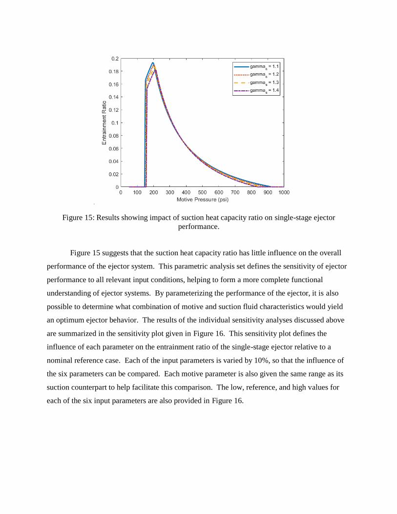
Figure 15: Results showing impact of suction heat capacity ratio on single-stage ejector
performance.
Figure 15 suggests that the suction heat capacity ratio has little influence on the overall
performance of the ejector system. This parametric analysis set defines the sensitivity of ejector
performance to all relevant input conditions, helping to form a more complete functional
understanding of ejector systems. By parameterizing the performance of the ejector, it is also
possible to determine what combination of motive and suction fluid characteristics would yield
an optimum ejector behavior. The results of the individual sensitivity analyses discussed above
are summarized in the sensitivity plot given in Figure 16. This sensitivity plot defines the
influence of each parameter on the entrainment ratio of the single-stage ejector relative to a
nominal reference case. Each of the input parameters is varied by 10%, so that the influence of
the six parameters can be compared. Each motive parameter is also given the same range as its
suction counterpart to help facilitate this comparison. The low, reference, and high values for
each of the six input parameters are also provided in Figure 16.

Figure 16: Sensitivity graph showing the influence of 10% changes to the input parameters.
Figure 16 shows the relative influence of each parameter on the entrainment ratio for the
single-stage ejector. There are a few conclusions that can be made from this graph. First, it is
advantageous to use a high stagnation temperature motive fluid. This can be attributed to the
increase in chemical energy with increasing temperature, as the energy contribution of the
motive fluid is the primary driver in pressure recovery within the ejector system. On the other
hand, the entrainment ratio capability of the single stage ejector decreases with increasing
suction stagnation temperature. The density of the suction fluid decreases with increasing
temperature, implying a reduction in momentum transfer between the suction and motive fluids
during mixing. Increasing the motive molecular weight acts to increase the motive mass flow
while simultaneously decreasing the velocity of the motive fluid during mixing. Both of these
factors decrease the entrainment ratio capability of the ejector, and this is supported by the
results given in Figure 16. In contrast, the entrainment ratio benefits from an increase in suction
molecular weight, indicating a preference toward high molecular weight suction fluids during
testing. Increases in both the motive and suction heat capacity ratios are shown to yield an
increase in entrainment ratio. However, this analysis implies that the performance of the ejector
is more responsive to changes in the motive heat capacity ratio when compared with suction heat
capacity ratio.
While this preliminary sensitivity analysis is useful for determining the fundamental
influence of each parameter on ejector performance, we also wanted to estimate the response of

entrainment ratio to these parameters over ranges which were more indicative of real world
testing conditions. The three motive fluids chosen as candidates for this second sensitivity
analysis were steam, argon, and air. The physical characteristics for each of these three
candidate fluids are summarized in the table below.
Table 3: Fluid characteristics for argon, steam, and air.
Motive Fluid Molecular Weight
[kg/kmol]
Heat Capacity
[J/(kg*K)]
Heat Capacity Ratio
Argon 39 520 1.67
Steam 18 2260 1.28
Air 28 1010 1.4
The range of motive stagnation temperatures for this sensitivity analysis were defined
based on the current fluid heating capabilities at ZL3 of Zucrow Labs. Ambient temperature was
defined as the lower bound for this analysis, while the upper bound of 800°F was defined based
on the maximum capability of the air heater at Zucrow Labs.
It was then necessary to determine the appropriate ranges for each suction parameter.
This was accomplished by running test cases with common propellant combinations using CEA.
For each of the test cases, a chamber pressure of 500 psia and an exit pressure of 5 psia was used.
The results for each of the evaluated test cases are given in Table 4. The results of the sensitivity
analysis using the bounds defined in Table 3 and Table 4 are given in Figure 17.
Table 4: Test cases evaluated to determine bounds for suction fluid parameters.
Oxidizer Fuel 𝑶/𝑭𝒐𝒑𝒕 Temperature
[K]
MW
[kg/kmol]
Heat
Capacity
[J/(kg*K)]
Heat
Capacity
Ratio
LOX RP-1 2.5 2056 24 2108 1.19
LOX LH2 4 1178 10 3699 1.29
LOX Methane 3 1879 21 2316 1.2
N2O4 UDMH 0.4 1743 24 1865 1.22

Figure 17: Sensitivity graph showing the influence of input parameters over real-world operating
ranges.
The large difference in variation for each of the parameters can be seen in Figure 17.
The results imply that the heat capacity ratio of the motive and suction fluids has a small impact
on ejector performance under real testing conditions. Suction temperature is shown to be the
most influential parameter on ejector performance, primarily due to its large operational range.
A high stagnation temperature and low molecular weight is shown to be the best combination for
the motive fluid. This result helps to explain why steam is frequently used as the motive fluid
for ejector systems in industry.
This procedural analysis was then modified to determine the sensitivity of simulated
altitude within the altitude chamber to these input parameters. While the previous analysis
describes the efficiency of the ejector system under different testing conditions, the treatment of
simulated altitude directly informs testing capabilities at various operating conditions. The real-
world bounds defined in Table 3 and Table 4 were used again, and the results of this final
sensitivity analysis are provided in Figure 18. This sensitivity analysis was performed assuming
a suction mass flow of 0.033 kg/s, which corresponds to a 100 Newton rocket with an Isp of 300
seconds.

Figure 18: Sensitivity graph showing the response of simulated altitude to each input parameter.
From Figure 18, suction stagnation temperature is shown to be the most influential
parameter for simulated altitude capabilities. The results again suggest that a high stagnation
temperature, low molecular weight motive fluid yields the highest simulated altitude. The
simulated altitude capability of the ejector is relatively insensitive to changes in both the motive
and suction heat capacity ratio. Each of these three individual sensitivity graphs helps us
develop a full understanding regarding the influence of each parameter on the testing capabilities
for the altitude facility.
Huang Model: Single-Stage Ejector Characterization Results
Following this parametrization of the ejector models, it was then necessary to validate the
Huang model using experimental data collected in-house. The results of this experimental model
validation were shown to necessitate a new, more simplistic, model which used fewer corrective
coefficients. An experimental testing campaign was conducted in the Spring of 2018 as part of a
class project for AAE 535, Propulsion Design Build Test. In this testing campaign, the class
group characterized the full operational range of the single-stage ejector. A picture of the single-
stage ejector is given in Figure 19, along with the relevant dimensions in the table following the
figure.

Figure 19: CAD rendering of single-stage ejector.
Table 5: Relevant dimensions of single-stage ejector.
# Dimension Value
(1) Suction Inlet Diameter (inch) 4
(2) Motive Inlet Diameter (inch) 2.5
(3) Pre-contraction Diameter (inch) 4.5
(4) Constant Section Diameter (inch) 2.25
(5) Diffuser Exit Diameter (inch) 4
(6) Contracting Length (inch) 10
(7) Constant Area Section Length (inch) 8
(8) Sub-sonic Expansion Length (inch) 12
(9) Total Length (inch) 42.5
As can be seen from the dimensions provided in Table 5, the single-stage ejector is
significantly smaller than the two-stage ejector characterized later in the thesis. However, it was
(1)
(2)
(6) (7) (8)
(5)
(4)
(3)
(9)

convenient to use this smaller single-stage ejector system to help validate the model introduced
by Huang et al. while the two-stage ejector system was being assembled. By collecting this
experimental data using a slightly smaller ejector, we hoped that the model could be validated so
as to predict the performance of the two-stage ejector in the future. Another part of the class
project was to characterize the performance of the ejector using three motive nozzles with
different expansion ratios. The relevant dimensions for the three motive nozzles are provided in
Table 6.
Table 6: Table displaying all relevant dimensions for the three nozzles.
Low ER Nozzle Original Nozzle High ER Nozzle
Throat Diameter (inch) 0.495 0.495 0.495
Exit Diameter (inch) 1.07 1.20 1.44
Total Length (inch) 4.15 4.15 4.15
Expansion Ratio (ER) 4.67 5.88 8.5
Each of the two new motive nozzles were machined from 316 Stainless Steel at the
Aerospace Sciences Laboratory (ASL) at Purdue University. This testing campaign made use of
facility nitrogen as the suction fluid and facility air as the motive fluid. A Plumbing and
Instrumentation Diagram (P&ID) describing the testing arrangement is given in Figure 20.

Figure 20: P&ID describing the experimental configuration for the performance characterization
of the single-stage ejector.
By varying the facility nitrogen stagnation pressure upstream of the venturi, we were able
to produce a full range of suction mass flow rates from 0 to 0.7 lbm/s of nitrogen. In the first
testing campaign, we characterized the performance of the single-stage ejector using the original
motive nozzle supplied by the manufacturer. The motive nozzle provided by the factory was
designed to achieve peak performance at a motive stagnation pressure of 215 psia. The primary
variables of interest for the experimental test were motive stagnation pressure, motive stagnation
temperature, suction mass flow rate, suction stagnation pressure, and suction stagnation
temperature. A motive nozzle isentropic efficiency of 0.993 was used for all experimental
testing campaigns. This was the same non-isentropic coefficient value used to calculate the
motive mass flow during experimental testing. The results for the first testing campaign using
the original motive nozzle are given in Figure 21.

Figure 21: Results from the first experimental testing campaign for single-stage ejector with
original motive nozzle.
A simplifying assumption made during analysis is that the motive and suction stagnation
temperatures remain unchanged over the course of the experimental test. For this reason, the
temperature of the motive/suction flows are not discussed within the context of the subsequent
analysis. There are a few conclusions that can be drawn from the experimental results. First,
increasing the stagnation pressure of the motive fluid improves ejector performance only to a
certain point. Increasing the motive stagnation pressure above the design pressure of 215 psia
yields no performance improvement for suction mass flow rates between 0 and 0.3 lbm/s, and it
yields only a minimal performance improvement for suction mass flow rates higher than
0.3 lbm/s. The experimental results for the two other nozzles are given in Figure 22 and Figure
23.

Figure 22: Graph of experimental results for 8.5 expansion ratio nozzle.
Figure 23: Graph of experimental results for 4.67 expansion ratio nozzle.
From the results shown in Figure 22, the pressure recovery capability of the ejector at
motive stagnation pressures below 215 psia suffers when compared with the original nozzle
geometry presented in Figure 21. However, the minimum suction pressure reached using the 8.5
expansion ratio nozzle at 215 psia is approximately 1.5 psia, as compared with 1.8 psia for the
original nozzle geometry. At the design pressure of 215 psia, the motive fluid expands just
enough to impinge with the walls of the constant-area section of the ejector. As the higher
expansion ratio nozzle yields a lower nozzle exit pressure, the suction pressure must decrease
accordingly to achieve the same optimum level of motive plume expansion. The inverse of this
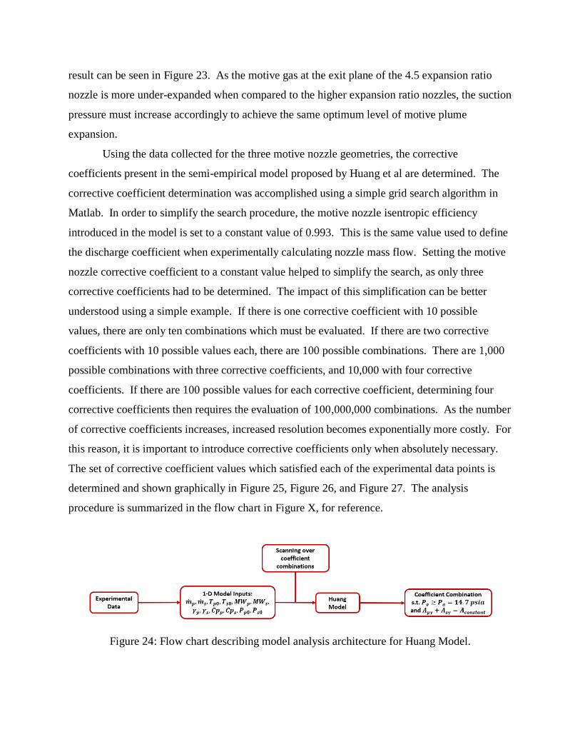
result can be seen in Figure 23. As the motive gas at the exit plane of the 4.5 expansion ratio
nozzle is more under-expanded when compared to the higher expansion ratio nozzles, the suction
pressure must increase accordingly to achieve the same optimum level of motive plume
expansion.
Using the data collected for the three motive nozzle geometries, the corrective
coefficients present in the semi-empirical model proposed by Huang et al are determined. The
corrective coefficient determination was accomplished using a simple grid search algorithm in
Matlab. In order to simplify the search procedure, the motive nozzle isentropic efficiency
introduced in the model is set to a constant value of 0.993. This is the same value used to define
the discharge coefficient when experimentally calculating nozzle mass flow. Setting the motive
nozzle corrective coefficient to a constant value helped to simplify the search, as only three
corrective coefficients had to be determined. The impact of this simplification can be better
understood using a simple example. If there is one corrective coefficient with 10 possible
values, there are only ten combinations which must be evaluated. If there are two corrective
coefficients with 10 possible values each, there are 100 possible combinations. There are 1,000
possible combinations with three corrective coefficients, and 10,000 with four corrective
coefficients. If there are 100 possible values for each corrective coefficient, determining four
corrective coefficients then requires the evaluation of 100,000,000 combinations. As the number
of corrective coefficients increases, increased resolution becomes exponentially more costly. For
this reason, it is important to introduce corrective coefficients only when absolutely necessary.
The set of corrective coefficient values which satisfied each of the experimental data points is
determined and shown graphically in Figure 25, Figure 26, and Figure 27. The analysis
procedure is summarized in the flow chart in Figure X, for reference.
Figure 24: Flow chart describing model analysis architecture for Huang Model.

Figure 25: Graph showing satisfactory suction coefficient values for motive pressure and suction
mass flow range of single-stage ejector.
Figure 26: Graph showing satisfactory motive plume coefficient values for motive pressure and
suction mass flow range of single-stage ejector.

Figure 27: Graph showing satisfactory mixing coefficient values for motive pressure and suction
mass flow range of single-stage ejector.
From the results given in Figure 25, there exists a discernable relationship between
suction coefficient, motive stagnation pressure, and suction mass flow rate. This relationship
allows for the development of a parametric curve fit which defines the value of the suction
coefficient over the operational range of the ejector; even between experimental data points.
However, there is no discernable trend for the motive plume and mixing coefficients. As a
result, it is not possible to reliably create a curve fit to define the value of these two coefficients.
This is an issue, as each of the three corrective coefficients must be well-defined over the full
operational range of the ejector. A large portion of time was spent trying to determine a
methodology to produce smooth, reliable results for these two coefficients, with no success.
Furthermore, evaluating the 165 experimental data points collected for the original
motive nozzle configuration took a relatively long time when compared to the final model
proposed within this thesis. Using a 1% resolution (100 points between 0 and 1) for each of the
three variable coefficients required nearly an hour of computational time. While this
computation time does not necessarily seem obstructively high, it is important to remember that
this model will eventually be used with a two-stage ejector system. Each of the two stages will
have these three corrective coefficients and will require a comparable level of resolution. This
means determining the performance of the two-stage ejector system will require roughly

1,000,000,000,000 combination evaluations for each experimental data point, as compared with
1,000,000 for a single-stage ejector system. This increase in evaluations will result in a
proportional increase in computational time, making this model infeasible at any reasonable level
of resolution. With these modeling results and conclusions in mind, a new model is created
which introduces only one corrective coefficient. The new model is successfully validated using
the same experimental data, and it produces smooth fittable curves for the included corrective
coefficient under a minute.
New Model: Overview
As many of the equations used in the new model are identical to those in the model
proposed by Huang et al., they are only introduced in the context of the new model. However,
mention is made of any equations which are derived from the previous model proposed by
Huang et al. The calculation procedure begins with the motive gas in the converging-diverging
nozzle of the ejector. Equation (7) is taken directly from the Huang Model, and it is used to
determine the mass flow of motive gas in the converging-diverging nozzle. The nozzle
isentropic efficiency is set to a constant value of 0.993, for reasons previously mentioned.
mp =Pp,0At
√Tp,0
√γp
Rp(
2
γp + 1)
(γp+1)(γp−1)
⁄
√ηp (7)
The Mach number at the exit plane of the motive converging-diverging nozzle is
determined using Newton’s method; the code supporting this calculation is given in the appendix
for reference. The determined Mach number can be used along with Equation (8) to determine
the static pressure at the exit of the motive converging-diverging nozzle. The static temperature
at the exit plane of the nozzle is determined using Equation (9). Equation (8) and Equation (9)
are shared with the Huang Model.
Pp1 = Pp0 (1 +γp − 1
2Mp1
2)
−γpγp−1
(8)

Tp1 = Tp0 (1 +γp − 1
2Mp1
2)−1
(9)
At this point in the model, an assumption is made that mixing between the motive and
suction fluids cannot begin until the motive and suction fluids are at equal pressure. If the
motive static pressure is higher than the suction static pressure, the motive Mach number is
recalculated using Equation (10). This equation is simply a manipulation of the isentropic
relation between static pressure and stagnation pressure, and it defines the Mach number
necessary for the motive static pressure to match the suction static pressure.
Mp2 = √2
γp − 1[(Pp1
Ps0)
γp−1
γp(1 +
γp − 1
2Mp1
2) − 1] (10)
The static temperature following this expansion can again be calculated using isentropic
relations. If the static pressure of the suction fluid is higher than that of the motive static
pressure, the suction Mach number is calculated using Equation (11).
Ms2 = √2
γs − 1[(Ps0Pp1
)
γs−1γs
− 1] (11)
The static temperature of the suction fluid is then determined using isentropic relations.
After determining the Mach numbers and static temperatures at the inlet of the control volume, it
is then necessary to determine the cross-sectional area for each of the two flows. The cross-
sectional area of the motive flow is determined using Equation (12); this equation is taken
directly from the Huang Model.

Ap2
Ap1=
Mp1 [2
γp + 1(1 +
γp − 12 Mpy
2)]
(γp+1)
(2(γp−1))⁄
Mp2 [2
γp + 1(1 +
γp − 12 Mp1
2)]
(γp+1)
(2(γp−1))⁄
(12)
It is assumed that mixing between the motive and suction fluids begins at the inlet to the
contracting section between the mixing chamber and constant-area section of the ejector; the
mixing between the two fluids occurs at equal pressure. As a result, the cross-sectional area of
the suction fluid is determined by subtracting the motive flow area from the area at the inlet to
the contracting section of the ejector.
As2 = Acontract − Ap2 (13)
The heat capacity, heat capacity ratio, and molecular weight of the mixed flow are
calculated as the weighted average of the motive and suction values. The calculation of these
three mixed values is accomplished using Equation (14), Equation (15), and Equation (16),
respectively.
Cp,mix =mpCp,p + msCp,s
mp + ms (14)
γmix =mpγp + msγs
mp + ms (15)
MWmix =mpMWp + msMWs
mp + ms (16)
The main control volume calculation present in the new model uses conservation of
energy and momentum to calculate the Mach number and static temperature of the mixed flow.
Equation (17) utilizes conservation of momentum to determine the resulting Mach number of the
mixed flow. A momentum coefficient is introduced into this equation to account for mixing
losses not captured in the equations of the new model; this is the only corrective coefficient
introduced within the model architecture.

PmixAmix(1 + γmixMmix2) = ηm[Pp2Ap2(1 + γpMp2
2) + Ps2As2(1 + γsMs22)] (17)
It was assumed previously that mixing between the motive and suction fluids occurs at
constant pressure. As a result, all of the pressure terms can be canceled out of the equation. It is
also assumed that the mixing process ends in the constant area section of the ejector. Isolating
Mmix yields Equation (18), given below.
Mmix = √ηmAp2
γmixAmix(1 + γpMp2
2) +ηmAs2γmixAmix
(1 + γsMs22) −
1
γmix (18)
Conservation of energy is then used, along with the calculated Mach number for the
mixed flow, to determine the mixed static temperature. Equation (19) is adapted from the Huang
Model, and it is a manipulation of the equation for conservation of energy.
��𝑚𝑖𝑥 (𝐶𝑝,𝑚𝑖𝑥𝑇𝑚𝑖𝑥 +1
2𝑉𝑚𝑖𝑥
2) = ��𝑝 (𝐶𝑝,𝑝𝑇𝑝2 +1
2𝑉𝑝2
2) + ��𝑠 (𝐶𝑝,𝑠𝑇𝑠2 +1
2𝑉𝑠2
2)
Tmix =mp (Cp,pTp2 +
12Mp2
2γpRpTp2) + ms (Cp,sTs2 +12Ms2
2γsRsTs2)
mmix (Cp,mix +12Mmix
2γmixRmix) (19)
It is assumed that a normal shock occurs in the constant-area section of the ejector after
mixing of the motive and suction fluids has concluded. The static pressure and Mach number of
the mixed flow following the normal shock can be calculated using Equation (20) and Equation
(21), respectively.
P3 = Pp22γmixMmix
2 − (γmix − 1)
γmix + 1 (20)
M3 = √(γmix − 1)Mmix
2 + 2
2γmixMmix2 − (γmix − 1)
(21)

The stagnation pressure at the exit plane of the ejector-diffuser is then calculated using
isentropic relations. The analysis procedure for the new model is summarized in the flow chart
given in Figure X.
Figure 28: Flow chart describing analysis procedure for new model.
New Model: Single-Stage Ejector Characterization Results
Once the new model had been developed, the momentum coefficient was experimentally
defined using the multi-nozzle test data collected earlier in the thesis. It is important that the
successful coefficient curve be smooth and fittable. A three-dimensional graph showing the
corrective coefficient value versus motive stagnation pressure and suction mass flow rate is
given in Figure 29 for the original nozzle configuration.
Figure 29: Graph of the momentum coefficient versus motive stagnation pressure and suction
mass flow for original nozzle.

The corrective coefficient curve in Figure 29 is smooth and fittable, allowing for the
designer to interpolate between experimental data points. This is a significant result, as this
means that the model can be used to accurately predict the performance of the single-stage
ejector system over its full operational range. Another interesting result present in Figure 29 is
the peak in efficiency that occurs around 220 psia. This aligns closely with the motive design
pressure for the single-stage ejector of 215 psia, and it implies that the new model accurately
absorbs the turbulent mixing behavior into the corrective coefficient. This behavior was unseen
in the Huang Model, implying that the model made assumptions which prevented the
visualization of this result. The new model was also validated using the experimental data from
the other two nozzle expansion ratios. The modeling results for these two experimental data sets
are given in Figure 30 and Figure 31.
Figure 30: Graph relating the momentum coefficient, motive stagnation pressure, and suction
mass flow for the 8.5 expansion ratio nozzle.

Figure 31: Graph relating the momentum coefficient, motive stagnation pressure, and suction
mass flow for the 4.67 expansion ratio nozzle.
Again, the experimental data yields fittable curves for the 4.5 and 8.5 expansion ratio
nozzles. It is shown that the model is robust enough to hold for multiple nozzle configurations.
Once the new model was validated using facility nitrogen and air as the motive and suction
sources, the model was then used to analyze the experimental results of a small solid rocket
motor test within the altitude chamber at reduced pressure.
New Model: Single-Stage Ejector Solid Rocket Motor Test Results
For this experimental test, we used an Aerotech F50 motor. The manufacturer provides a
thrust profile for the motor, which can be imported into Matlab to determine the mass flow
profile for the motor. The full list of specifications relating to the Aerotech F50-9T motor is
given in Table 7 below. The thrust curve for the F50 motor is given in Figure 32, and it is used
to determine the average Isp for the solid rocket motor.

Table 7: Specifications for Aerotech F-50 solid rocket motor [32].
Parameter Value
Total Propellant Mass (g) 54
Burn Duration (s) 1.4
Exit Temperature (K) 1500
Molecular Weight (g/mol) 23.04
Specific Heat Ratio 1.28
Figure 32: Graph of the thrust profile for the Aerotech F50-9T solid rocket motor [32].
The mass flow for a chosen average Isp can be calculated using the fundamental rocket
thrust equation. An average Isp of 130 seconds was determined for the motor, as this yielded a
total propellant mass flow of approximately 54 grams. This exhaust mass flow curve is
calculated using the provided thrust curve and average specific impulse, and it is overlaid with
the experimental suction stagnation pressure response in Figure 33.
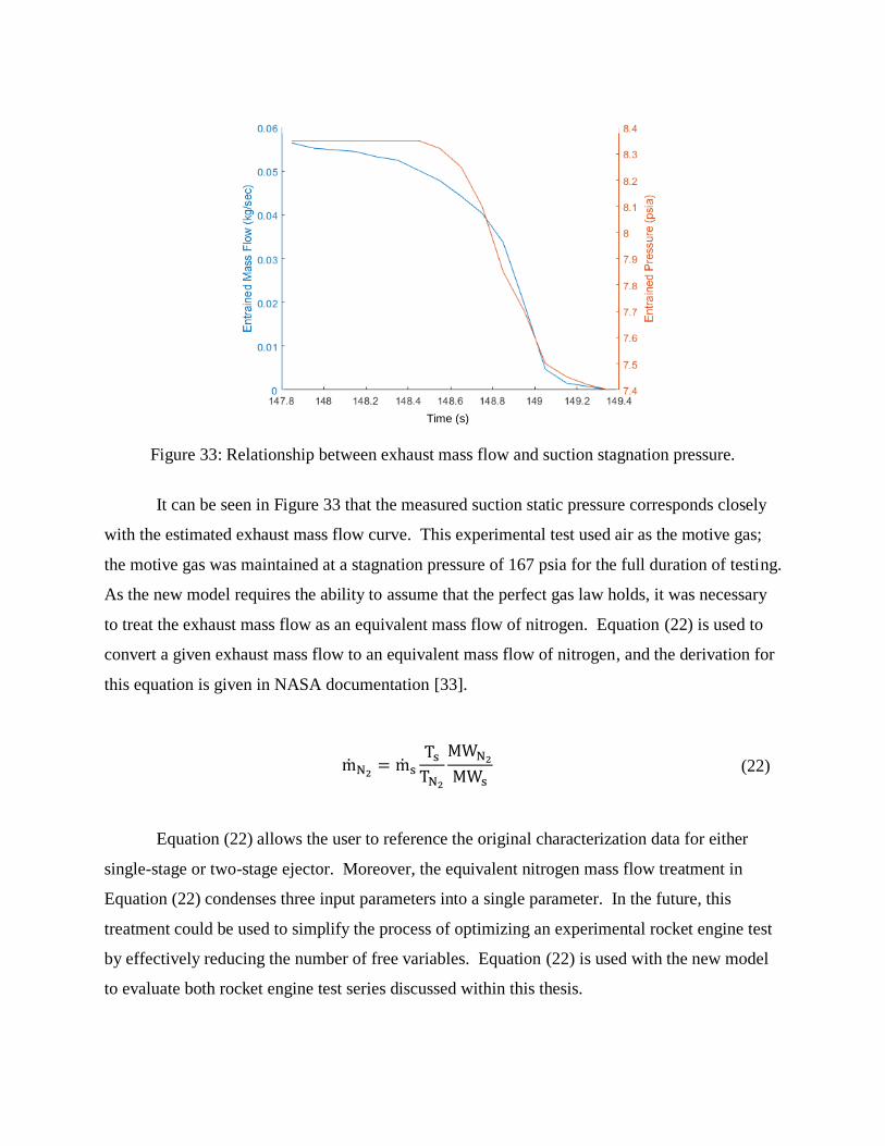
Figure 33: Relationship between exhaust mass flow and suction stagnation pressure.
It can be seen in Figure 33 that the measured suction static pressure corresponds closely
with the estimated exhaust mass flow curve. This experimental test used air as the motive gas;
the motive gas was maintained at a stagnation pressure of 167 psia for the full duration of testing.
As the new model requires the ability to assume that the perfect gas law holds, it was necessary
to treat the exhaust mass flow as an equivalent mass flow of nitrogen. Equation (22) is used to
convert a given exhaust mass flow to an equivalent mass flow of nitrogen, and the derivation for
this equation is given in NASA documentation [33].
mN2 = ms
TsTN2
MWN2
MWs (22)
Equation (22) allows the user to reference the original characterization data for either
single-stage or two-stage ejector. Moreover, the equivalent nitrogen mass flow treatment in
Equation (22) condenses three input parameters into a single parameter. In the future, this
treatment could be used to simplify the process of optimizing an experimental rocket engine test
by effectively reducing the number of free variables. Equation (22) is used with the new model
to evaluate both rocket engine test series discussed within this thesis.
Time (s)
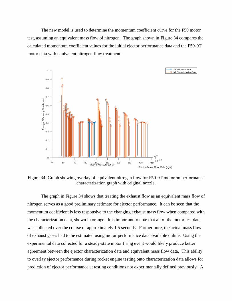
The new model is used to determine the momentum coefficient curve for the F50 motor
test, assuming an equivalent mass flow of nitrogen. The graph shown in Figure 34 compares the
calculated momentum coefficient values for the initial ejector performance data and the F50-9T
motor data with equivalent nitrogen flow treatment.
Figure 34: Graph showing overlay of equivalent nitrogen flow for F50-9T motor on performance
characterization graph with original nozzle.
The graph in Figure 34 shows that treating the exhaust flow as an equivalent mass flow of
nitrogen serves as a good preliminary estimate for ejector performance. It can be seen that the
momentum coefficient is less responsive to the changing exhaust mass flow when compared with
the characterization data, shown in orange. It is important to note that all of the motor test data
was collected over the course of approximately 1.5 seconds. Furthermore, the actual mass flow
of exhaust gases had to be estimated using motor performance data available online. Using the
experimental data collected for a steady-state motor firing event would likely produce better
agreement between the ejector characterization data and equivalent mass flow data. This ability
to overlay ejector performance during rocket engine testing onto characterization data allows for
prediction of ejector performance at testing conditions not experimentally defined previously. A

flow chart is provided in Figure 35 to show how this equivalent nitrogen treatment could be used
to predict the performance of an ejector at new testing conditions.
Figure 35: Flow chart displaying procedure for using characterization data and equivalent
nitrogen flow treatment to extend model prediction capabilities.
As this result only shows that equivalent nitrogen mass flow treatment is viable at the
operating conditions relevant to the F50-9T motor test, subsequent tests were performed using
motors with different exhaust products and temperatures. These subsequent tests were also
performed using the two-stage ejector system to maintain a reduced pressure environment within
the altitude chamber. Modifications had to be made to the modeling script to allow for the
characterization of a two-stage ejector system. This modification was relatively easy, as the
inlet and exit conditions for each of the two ejector stages are known. As a result, each stage of
the ejector system can be characterized separately.
New Model: Two-Stage Ejector Characterization Results
Before the next motor test could be analyzed using the new model, it was necessary to
calibrate the model for the two-stage ejector system. An experimental test similar to that for the
single-stage ejector system was performed to characterize the performance of the two-stage
ejector over its relevant operational range. A CAD rendering of the two-stage ejector on loan
from NASA Marshall is given in Figure 36. The relevant dimensions for the two-stage ejector
system are given in Table 8.
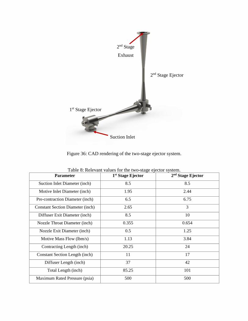
Figure 36: CAD rendering of the two-stage ejector system.
Table 8: Relevant values for the two-stage ejector system. Parameter 1st Stage Ejector 2nd Stage Ejector
Suction Inlet Diameter (inch) 8.5 8.5
Motive Inlet Diameter (inch) 1.95 2.44
Pre-contraction Diameter (inch) 6.5 6.75
Constant Section Diameter (inch) 2.65 3
Diffuser Exit Diameter (inch) 8.5 10
Nozzle Throat Diameter (inch) 0.355 0.654
Nozzle Exit Diameter (inch) 0.5 1.25
Motive Mass Flow (lbm/s) 1.13 3.84
Contracting Length (inch) 20.25 24
Constant Section Length (inch) 11 17
Diffuser Length (inch) 37 42
Total Length (inch) 85.25 101
Maximum Rated Pressure (psia) 500 500
1st Stage Ejector
2nd Stage Ejector
Suction Inlet
2nd Stage
Exhaust

The two-stage ejector was only experimentally characterized at its full-flow state, with
the 1st and 2nd stage motive stagnation pressure set at the maximum rated pressure of 500 psia.
This is primarily because there are no plans to supply less than 500 psia to each of the two stage
during the experimental testing of rocket engines within the altitude chamber. For this reason,
all modeling results assume a constant motive stagnation pressure of 500 psia for each of the two
stages. The experimentally measured relationship between 1st stage suction mass flow rate and
1st stage suction stagnation pressure is given in Figure 37.
Figure 37: Relationship between 1st stage suction stagnation pressure and 1st stage suction mass
flow rate for two-stage ejector system.
From the graph in Figure 37, there is an approximately quadratic relationship between the
suction mass flow rate and suction stagnation pressure for the 1st stage ejector. Due to
limitations on facility air usage, we were unable to characterize the full operational range of the
two-stage ejector at its full-flow state. However, the presence of this approximately quadratic
relationship could allow for extrapolation to higher suction mass flow rates, if the need arises.
The new model was then used to evaluate the experimental characterization data set for
the two-stage ejector. The primary motivation for this modeling step was to ensure that the
performance of the two-stage ejector could still be captured by the new model. The modeling
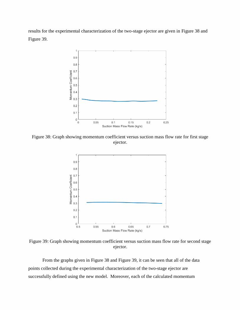
results for the experimental characterization of the two-stage ejector are given in Figure 38 and
Figure 39.
Figure 38: Graph showing momentum coefficient versus suction mass flow rate for first stage
ejector.
Figure 39: Graph showing momentum coefficient versus suction mass flow rate for second stage
ejector.
From the graphs given in Figure 38 and Figure 39, it can be seen that all of the data
points collected during the experimental characterization of the two-stage ejector are
successfully defined using the new model. Moreover, each of the calculated momentum

coefficient curves are smooth and fittable, allowing for interpolation between experimental data
points. It can also be seen in Figure 38 and Figure 39 that the momentum coefficient curves are
relatively constant when compared to the modeling results for the single stage ejector, shown in
Figure 29. This is due to the limited range of the characterization data for the two-stage ejector.
Performing a more complete experimental characterization of the two-stage ejector over its full
operational range would help further inform the modeling results, as well as avoid extrapolation.
New Model: Two-Stage Ejector 90 Newton Rocket Engine Test Results
Once it was determined that the new model could successfully capture the performance
of the two-stage ejector, the new model was evaluated using rocket engine test data. The results
of this modeling step would help to determine whether the new model is a viable predictive tool
to be used with the two-stage ejector system. The relevant rocket exhaust flow conditions for the
experimental test to be evaluated using the new model are given in the table below. While the
exhaust temperature and molecular weight are approximately values, they are shown to be
sufficient in proving the viability of the new model as a predictive tool for the testing of rocket
engines using the two-stage ejector system.
Table 9: Relevant flow conditions for the rocket engine test using the two-stage ejector.
Parameter 1st Stage Ejector
Suction Temperature (K) 1000
Suction Molecular Weight (kg/kmol) 22
Suction Heat Capacity Ratio 1.3
Suction Mass Flow Rate (lbm/s) 0.106
Suction Pressure (psia) 1.4
Similar to the treatment of the rocket exhaust mass flow in the single-stage modeling, the
rocket exhaust mass flow is converted into an equivalent mass flow of nitrogen. The calculated
momentum coefficient values for the two ejector stages resulting from this equivalent nitrogen
mass flow treatment is then overlaid on the momentum coefficient curves derived from the
experimental characterization data. This visual comparison between the momentum coefficient
values for the equivalent nitrogen mass flow treatment and experimental characterization data is
presented in Figure 40 and Figure 41.

Figure 40: Comparison on momentum coefficient value between characterization data and
equivalent nitrogen flow for rocket engine test for 1st stage ejector.
Figure 41: Comparison on momentum coefficient value between characterization data and
equivalent nitrogen flow for rocket engine test for 2nd stage ejector.
From the results given in Figure 40 and Figure 41, it can be seen that there is generally
good agreement between the ejector characterization data and equivalent nitrogen mass flow

treatment of the rocket exhaust. In this way, it is shown that the equivalent nitrogen mass flow
methodology can be implemented with reasonable accuracy to predict the performance of both
the single-stage and two-stage ejector systems during the testing of rocket engines at reduced
pressure.
Graphical User Interface: Overview
In an effort to improve accessibility, a simple graphical user interface (GUI) was created
to allow the user to input suction and motive flow conditions relevant to their desired testing
conditions for either the single-stage and two-stage ejector system. There also exists the option
to input characterization data for alternate ejector geometries, further extending the predictive
capabilities of the new 1-D model. The general procedure for using the GUI is provided below
for reference.
Figure 42: Screen of model GUI used to specify the number of ejector stages used.
This page of the GUI is relatively straightforward, requiring only the number of desired
number of ejector stages for the evaluation. Currently, only single-stage and two-stage ejectors
are available. This GUI also only treats multi-stage ejector configured in series. This is because
the GUI is set up to handle only ejector for which we already have characterization data.

Figure 43: Screen of model GUI used to specify 1st stage suction flow values.
Figure 43 is used to specify whether or not you are evaluating a rocket engine test. After
choosing one of the two options, you can then specify all of the relevant entrained flow
conditions. This section of the GUI also has a built-in function which can run Chemical
Equilibrium with Application (CEA). After specifying all of the relevant entrained conditions,
Figure 44 is used to define the 1st stage motive flow conditions and ejector dimensions.
Figure 44: Screen of model GUI used to specify 1st stage motive flow values.

The section of the GUI given in Figure 44 is used to specify the motive conditions and
geometrical dimensions relevant the 1st stage ejector. This includes the constant section
diameter, pre-contraction diameter, and nozzle geometry. If a two-stage system was specified in
Figure 42, then Figure 45 is displayed.
Figure 45: Screen of model GUI used to specify 2nd stage motive flow values.
The inputs for the 2nd stage motive conditions and geometrical dimensions are identical to
those given in Figure 44. Once this section is completed, the model can be evaluated for what
ejector options were chosen in the GUI. This GUI serves as a preliminary tool to meet basic
ejector modeling needs. However, the complexity of this GUI, as well as the complexity of the
new model, can be revised as necessary. In this way, the new model and GUI serve as a
foundation on which to build increasingly accurate modeling architectures.
While not modeled within the context of this thesis, the new hybrid rocket engine
designed as part of a collaborative effort between Zucrow Labs and JPL is scheduled to test in
the altitude chamber in late July of this year. This will be the first major testing campaign that
occurs within the altitude chamber following the completion of this thesis. As the new JPL
motor is optimized for 90 lbf at 100,000 ft, it is essential that the performance of the two-stage
ejector in ZL3 be well understood. The design of the new JPL motor began in mid-January of
this year, and it is discussed in detail in the following section.

5 JPL MOTOR DESIGN
Over the last five years, Dr. Pourpoint’s research group has collaborated with JPL to
characterize the performance of a hybrid motor design, which could potentially be used for the
Mars Ascent Vehicle (MAV) mission. One of the major constraining factors in propellant choice
is the ambient temperature on the surface of Mars, roughly -55°C. This motivated the use of a
hybrid propulsion architecture with a solid fuel and an oxidizer with a freezing point well below
this average temperature. The oxidizer of interest in the project was Mixed Oxides of Nitrogen
(MON). There are two main constituents of MON: nitric oxide (NO) and nitrogen tetroxide
(N2O4). While nitrogen tetroxide has a relatively high freezing point of around -10°C, this
freezing point can be depressed by introducing nitric oxide. Mixing nitric oxide with nitrogen
tetroxide acts to lower the overall freezing point of the mixture, making this mixture a viable
propellant candidate for use in the MAV mission.
The concentration of nitric oxide introduced into nitrogen tetroxide is measured on a
mass basis, and is denoted in the number following MON. For example, a mixture of Nitrogen
Tetroxide and 25% by weight of Nitric Oxide is denoted as MON-25. It has been shown in
literature than MON-25 has a freezing point around -55°C [34]. For this reason, MON-25 has
been pursued as a potential propellant to be used on the Mars Ascent Vehicle (MAV) project in
collaboration with JPL. Though characterization of the hybrid configuration was initially
performed at sea-level conditions [35], it is more representative to test the hybrid motor in a
reduce pressure environment corresponding more closely to the Martian atmosphere.
A new motor design is proposed for testing at reduced pressures within the altitude
chamber to closely represent atmospheric conditions experienced on Mars. The functional and
performance requirements for the new JPL motor are given on the next page.

Functional Requirements:
• Ease of cleaning/disassembly
• Design failure model for safety
• 2 to 5 second firing duration
• Combustion chamber pressure/temperature measurement capability
• Expendable components of standard dimensions
Performance Requirements:
• 600 psia over-pressurization threshold with safety factor > 3 for all components
o 200-300 nominal operating pressure
• 0.1 lbm/s MON flow rate
• ~0.01 lbm/s liquid igniter/N2 flow rate prior to steady operation
• 90 lbf thrust
While these functional and performance requirements acted to guide much of the design
process, there were additional factors which served to further constrain the potential design
space. There are unique challenges inherent to the testing of a motor in an altitude chamber at
reduced pressure. First, there is a limited number of flanges on the altitude chamber. Many of
these flanges are already used for optical access for recording tests and optical measurement of
the flow, and for thermocouple and pressure transducer feedthroughs. For this reason, it is
beneficial to design a motor which minimizes the number of necessary feedthroughs outside of
basic pressure and temperature instrumentation. MON-25 is extremely corrosive, requiring the
motor to be made of materials which are compatible with this oxidizer. 316 stainless steel has
been shown to be chemically compatible with MON-25, and it is thus chosen to be the material
for the main body of the motor. A final implicit requirement was that the new JPL motor had to
be able to accept the existing grain geometry used for atmospheric tests.
The design of a new system capability is inherently iterative in nature, with all associated
elements being subject to change over time. These changes are reflected in both the system
design and the overarching design requirements which guide the project. One should not expect
to arrive at the optimal solution with the first design concept. Instead, the initial conceptual
design serves only as a benchmark by which to compare subsequent designs. With each iteration

of design, the team slowly converges on the optimal solution by resolving shortcomings present
in the previous design iterations. It is the task of the designer to efficiently utilize all relevant
expertise to ensure that the design process continues to converge on the optimal solution.
The design decisions made in this project were highly transparent and involved all relevant
faculty and staff at the Zucrow Labs and engineers at the National Aeronautics and Space
Administration (NASA) and the Jet Propulsion Laboratory (JPL). All significant changes made
to the design were presented to NASA/JPL, and appropriate revisions were determined and
implemented. Though there exist roughly eight iterations for the design of the new JPL motor
for reduced-pressure testing, only the final iteration is discussed within the context of this thesis.
There are five major components relating to the design of the JPL motor: CAD design; FEA
analysis and stress analysis; thermal expansion analysis; thermal stress analysis; and shear pin
design. Each of these five components of the design process will be detailed in this section of
the thesis.
The first step is to create a three-dimensional model, which helps to visually determine the
impact of decisions made throughout the design process. This is accomplished using Computer
Aided Design (CAD); Solidworks 2019 is used to create all of the CAD models presented within
this thesis. Some aspects of the design were fixed or constrained at the beginning of the design
process. For example, the combustor had to accommodate the same grain configuration used in
the previous JPL motor for atmospheric performance characterization. The new combustor also
had to use the same spray injector present in the atmospheric testing campaign, as the flow
behavior and performance of the old spray injector was already experimentally validated.
It is also important to design a motor that minimizes the probability of a catastrophic over-
pressurization event occurring. There are multiple mechanisms by which this over-
pressurization can occur, including blockage of the nozzle throat, high ignition delay, and de-
bonding of the fuel grain within the combustion chamber. The concept of over-pressurization
varies from motor to motor and defines the upper pressure threshold that is tolerable for the
given motor configuration. If the pressure within the motor rises above this upper threshold,
there must exist a reliable mechanism to quickly relieve pressure. Otherwise, there is a high
likelihood that the entire motor will be lost.
In design, it is often beneficial to define a factor of safety for each component of the motor.
A factor of safety is the ratio of the maximum stress experienced to the maximum stress that the

component can withstand. The maximum allowable stress for a given component depends on the
component geometry, as well as its material composition. The desired factor of safety for a
system can vary widely depending on the risk threshold for the mission or application. For
instance, a factor of safety of 1.4 to 1.5 is often desirable for flight-ready systems [36]. Flight-
ready systems are generally designed with a lower factor of safety to optimize operational
performance. Increasing the amount of stress that a component can withstand often means
increasing wall thicknesses or using exotic materials. These two factors serve to increase the
cost of the final flight system, and also potentially reduce the relative performance of the system
through an increase in overall weight. For non-flight systems, it is often advantageous to have a
higher safety factor. The increase in weight and cost is less significant for non-flight systems,
and thus priority can shift toward minimizing associated operational risks. It will be shown that
each component of the motor designed within the context of this thesis has a factor of safety of at
least 2, aside from the nozzle insert. The reasoning for the slightly lower factor of safety for the
nozzle insert will be explained later in the thesis.
The CAD model is composed of seven major components: injector housing, injector flange,
main pipe section, main pipe partial, nozzle housing and expansion section, nozzle insert, and
shear pins. Each of these components will first be discussed in detail individually. The inter-
relations between these components will then be discussed, culminating in the final discussion of
the motor as a whole. There are also smaller supporting components associated with the motor
design which will be discussed as appropriate.
Injector Assembly Design
The injector housing is the upstream-most component of the motor and supports oxidizer,
igniter, and nitrogen injection into the combustion chamber of the motor. A CAD model
depicting the overall geometry of the injector housing is given in Figure 46 to support the
proceeding discussions.

Figure 46: CAD model cutaway view showing all major design components of injector housing,
as well as the full-cone spray injector.
As can be seen in Figure 46, there are three main ports which support the injection of three
different fluids into the motor. The larger ¼ inch diameter port in the center supports the main
flow of MON-25, and feeds into a full-cone spray injector. There are two smaller 1/8 inch ports
which feed an annular injection ring; one of these ports is for the nitrogen purge, and the other is
for the igniter liquid. As the fuel grain includes moisture sensitive additives, it is necessary to
continuously purge the grain with nitrogen before and after firing. Igniter injection is included to
help ensure successful ignition in the new reduced-pressure testing environment within the
altitude chamber. The full injector assembly, which includes both the injector housing and
injector flange, is shown in Figure 47.
0.5 inch

Figure 47: CAD model depicting full injector assembly.
In Figure 47, the injection holes in the injector flange are clocked 90° from the nitrogen and
igniter ports in the injector housing. The design of these injection holes is discussed later in this
section of the thesis. This 90° clocking ensures that each of the two injection holes receives an
equal flow rate of both nitrogen and igniter fluid from the upstream injection ports. The injector
housing and injector flange are machined as two separate parts to aid in machinability,
adaptability, and ease of cleaning. If an annular ring were not included in the design, each
injection hole would have to be fed by individual ports in the injector housing. While this is not
necessarily an issue with only two injection holes, it would quickly become problematic as the
number of injection holes increased. As the injector assembly is composed of two parts, a
change in injection hole configuration only requires redesigning the injector flange. This saves
in long term design/machining costs, and also allows for ease of access for cleaning the annular
ring.
In addition to supporting the injection of relevant testing fluids into the combustion chamber,
the injector flange also supports the measurement of the combustion chamber pressure and
temperature. There are four 1/8 inch instrumentation ports machined into the injector flange;
these are shown in Figure 48 for reference.
0.5 inch

Figure 48: CAD cutaway view showing instrumentation ports in the injector flange used for
combustion chamber pressure and temperature measurement.
Dividing the injector assembly into two components necessitated the addition of two sealing
O-rings between the injector flange and injector housing. The inner O-ring acts to prevent the
mixing of MON-25 and the igniter fluid. The outer O-ring is designed to prevent the igniter
fluid, as well as combustion gases, from leaking into the altitude chamber. The sizing of these
two O-ring grooves, and all other O-ring grooves on the motor, was completed using the Parker
O-ring handbook [37]. It was essential that the O-rings were compatible with MON-25, as they
would be exposed to the main oxidizer flow during testing. Polytetrafluoroethylene (PTFE) is
known to be compatible with MON-25, and thus PTFE was chosen as the O-ring material.
In the design requirements, a 10% mass flow of igniter fluid relative to the main MON-25
flow is desired. As the main MON-25 mass flow is roughly 0.1 lbm/s, the injection holes are
design to support a total igniter flow rate of roughly 0.01 lbm/s. It is also important to have an
adequate pressure drop across the injection holes, in order to prevent the flow of combustion
gases back into the annular ring. For our implementation, a desired pressure drop of roughly
100 psia was defined. Equation (23) is used to determine the size and number of injection holes
necessary to achieve this desired mass flow and pressure drop.
∆P =1
2ρ(
m
NCdA)2
(23)
1 inch

A 114 psia theoretical pressure drop was achieved using two 0.012 inch diameter injection
holes. These small diameter holes were produced using EDM drilling methods and satisfied both
our mass flow and pressure drop criteria.
A flange outer diameter of 6 inches and a flange thickness of 0.75 inch was chosen for each
of the four flanges on the motor. The outer diameter for each flange was only constrained by the
geometry of the motor components. It was desirable to minimize the outer diameter of the
flanges, as this would equate to less raw material and machining cost. However, there also had
to be enough space for the bolts to slide into the bolt holes. The main driving constraint for the
minimum diameter of the flanges was the injector housing. The outer diameter of the injector
housing is roughly 4 inches, approximately 1 inch larger than the outer diameter for all other
motor components. A flange outer diameter of 6 inches ensured that there were no interference
issues between the connecting bolts and the body of the motor. Equation (24) is used to validate
the thickness for all flanges on the motor.
σ = P(Dflange
Tflange)
2
(24)
A safety factor is defined as the ratio of the calculated stress in the component to the yield
strength of the material. As mentioned in the performance requirements provided by JPL, our
factor of safety is defined relative to a chamber pressure of 600 psia. This is much higher than
the chamber pressure expected during nominal motor operation, and it represents the critical
point at which the pressure within the combustion chamber must be relieved. A relief mechanism
in the form of a free floating nozzle insert held in place by graphite shear pins is included in the
motor design to ensure that the pressure within the combustion chamber of the motor does not
rise above this 600 psia threshold. As a result, all of the safety factors defined in the design
process denote the ratio of the stress experienced in the component for a chamber pressure of 600
psia to the maximum allowable stress for that part. For a chamber pressure of 600 psia, the
maximum stress in the motor flanges given a flange thickness of ¾ inch was 9,700 psi. As the
yield strength of 316 Stainless Steel is approximately 30,000 psi, this yielded a safety factor of
over 3 for the thickness of the flanges used on the motor.

Main Pipe Section/Partial Design
The next step was to determine the necessary wall thickness for the main pipe section and
main pipe partial. This was accomplished first using basic hoop stress calculations. There are
two main regimes for calculating hoop stress: thin-walled and thick-walled. The thin-walled
assumption is appropriate if the ratio of the outer diameter to inner diameter is less than 1.1,
while the thick-walled assumption is appropriate if this ratio is greater than 1.5. The main pipe
section has a ratio value of approximately 1.33. The safety factor for the main pipe section and
main pipe partial are calculated using both assumptions, and the results of these two assumptions
are compared. Equation (25) defines the stress in the pipe using the thin-walled assumption, and
Equation (26) defines the stress in the pipe using the thick-walled assumption.
σ =0.5PDin
t (25)
σ = PDout
2 + Din2
Dout2 − Din
2 (26)
The calculated stress using the thin-walled assumption was roughly 2,800 psi, and the
calculated stress using the thick-walled assumption was roughly 3,100 psi. In our case, 316
stainless steel was utilized as the material for the main pipe section and main pipe partial. This
yields a safety factor of 11 using the thin-walled assumption and 10 using the thick-walled
assumption. This is more than sufficient for our purposes, and thus we move on to the next steps
in the design process.
It was determined that the center body of the motor, which holds the phenolic case and fuel
grain, needed to be modular, allowing for different grain configurations to be evaluated with
various post-combustion chamber lengths. For this reason, the center body of the motor was
divided into two sections: main pipe section and main pipe partial. By removing main pipe
partial, and cutting a shorter phenolic case length, the motor could be tested with a shortened
post-combustion chamber. The two proposed configurations are given in Figure 49 below, with
and without main pipe partial.

Figure 49: CAD cutaway view showing the normal and shortened motor configurations.
One important step in the design process is to determine the bolt sizes necessary to prevent
point failures at flanged connections. Both tensile stress and bolt shear stress calculations were
performed for the bolted connections between the injector housing and injector flange, as well as
between the injector flange and main pipe section. While there are two other flanged
connections on the motor (main pipe section – main pipe partial and main pipe partial – nozzle
housing/expansion section), these use the same flanges and bolted connections as between the
injector flange and main pipe section. A factor of safety can again be defined here based on the
tensile and shear strength of the material, Grade-8 steel in this case for all of the bolts. Again, a
pressure of 600 psia is used in this calculation to represent the maximum pressure threshold for
the motor. Equation (27) is used to calculate bolt shear stress, and Equation (28) is used to
calculate bolt tensile stress. There is one term in Equation (28), called the bolt tensile area,
which must be calculated separately using Equation (29).
3 inches

σ =P(Do
2)
Le(E)(N) (27)
σ =π4⁄ PDo
2
AtN (28)
At =π
4(Dm − 0.938194p)2 (29)
It was determined that eight ¼”-20 bolts were sufficient to connect the injector housing and
injector flange. This number and size of bolts yields a factor of safety of 9 for bolt tensile shear,
and a factor of safety of 8 for bolt thread shear. 3/8”-16 bolts were chosen for the three main
flanged connections on the motor. This yields a factor of safety of 22 for bolt tensile shear, and a
factor of safety of 23 for bolt thread shear. Once the bolt sizes and numbers are determined, we
move onto the design of the nozzle housing/expansion section.
Nozzle Assembly Design
The nozzle housing/expansion section, and the nozzle insert, were designed simultaneously.
A CAD model showing the final geometry of the nozzle housing/expansion section and nozzle
insert is given in Figure 50.
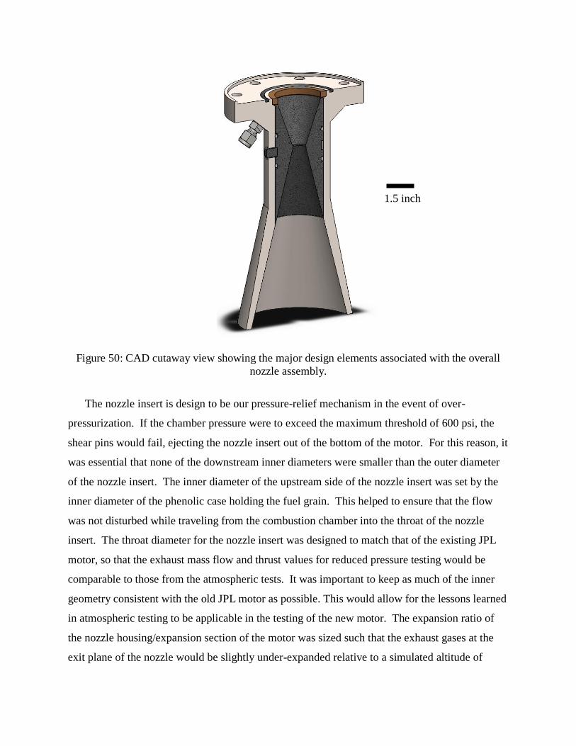
Figure 50: CAD cutaway view showing the major design elements associated with the overall
nozzle assembly.
The nozzle insert is design to be our pressure-relief mechanism in the event of over-
pressurization. If the chamber pressure were to exceed the maximum threshold of 600 psi, the
shear pins would fail, ejecting the nozzle insert out of the bottom of the motor. For this reason, it
was essential that none of the downstream inner diameters were smaller than the outer diameter
of the nozzle insert. The inner diameter of the upstream side of the nozzle insert was set by the
inner diameter of the phenolic case holding the fuel grain. This helped to ensure that the flow
was not disturbed while traveling from the combustion chamber into the throat of the nozzle
insert. The throat diameter for the nozzle insert was designed to match that of the existing JPL
motor, so that the exhaust mass flow and thrust values for reduced pressure testing would be
comparable to those from the atmospheric tests. It was important to keep as much of the inner
geometry consistent with the old JPL motor as possible. This would allow for the lessons learned
in atmospheric testing to be applicable in the testing of the new motor. The expansion ratio of
the nozzle housing/expansion section of the motor was sized such that the exhaust gases at the
exit plane of the nozzle would be slightly under-expanded relative to a simulated altitude of
1.5 inch

100,000 ft. This would allow the exhaust gases to continue expanding, eventually impinging
with the walls of the downstream supersonic diffuser inlet. For a nozzle throat diameter of
0.6 inch an exit diameter of 4.45 inches was chosen to yield an exit pressure of approximately
0.25 psia. This theoretical exit pressure was determined using CEA with propellant and chamber
values relevant to the testing of the new JPL motor, and it represents an equivalent altitude of
approximately 91,000 ft.
Nozzle Assembly Thermal Analysis
An axisymmetric thermal analysis was performed for the nozzle housing/expansion section,
phenolic ring, and nozzle insert. The heat transfer was determined using results from CEA and
the Dittus-Boelter Correlation, which is given in Equation (30) for reference.
NuD = 0.023Re0.8Pr0.4 (30)
The heat transfer was determined at three discrete locations within the model geometry:
combustion chamber, nozzle throat, and exit of the expansion section. The heat transfer values
were then interpolated between these three points to define the heat transfer distribution along
the entire nozzle geometry. The thermal analysis was performed for a 2 second test, as well as
for a 5 second test. While most of the atmospheric tests were around 2 seconds in length, it was
essential to design the motor to support whatever testing conditions might arise in the future.
The thermal analysis results for the 2 and 5 second firing durations are given in Figure 51.

Figure 51: COMSOL thermal analysis result for 2 and 5 second firing durations without TBC.
From the results in Figure 51, it became clear that the proposed motor configuration would
not survive without the addition of a thermal barrier coating. The melting temperature of 316
stainless steel is approximately 2550°F, while the maximum temperature experienced during
even the 2 second test is 2600°F. A thermal barrier coating (TBC), made of Zirconia and an 8%
weighting of Yttria-Oxide, was included in an updated thermal analysis. The thickness of each
portion of the thermal barrier coating is given in Figure 52.
Tmax = 3300°F Tmax = 2600°F

Figure 52: Thicknesses and locations of TBC application.
After adding the thermal barrier coating in the necessary locations, the thermal analysis was
once again performed. The results for the 2 second and 5 second firing durations with thermal
barrier coating included are given in Figure 53.
1 inch

Figure 53: Thermal analysis results for 2 and 5 second firing durations with TBC.
From the results of this analysis, it can be seen that the maximum temperature experienced
by the 316 stainless steel components is well below the melting temperature of the material. The
thermal analysis also defined the maximum temperature that the nozzle insert O-rings would
experience during the two firing durations. The maximum temperature experienced by the
nozzle-insert O-rings for each of the two firing durations is shown in Figure 53 above. For a
firing duration of 5 seconds, the maximum temperature experienced by the nozzle insert O-rings
is approximately 440°F. While this is the maximum rated temperature for silicon O-rings,
silicon does not deform or melt under momentary temperature loads. Furthermore, both nozzle
insert O-rings will be changed out at the end of every test. For these reasons, we continued on to
the next steps in the design process.
The design of the nozzle housing/expansion section and nozzle insert was perhaps the most
difficult part of the design process. In order to protect the shear pins during testing, O-ring
grooves were designed upstream and downstream of the shear pin groove in the nozzle insert.
There was a maximum allowable diametrical clearance between the outer diameter of the nozzle
insert and inner diameter of the nozzle housing/expansion section. The maximum diametrical
clearance is defined in the extrusion limits section of the Parker O-ring Handbook [37]. The
graph used for this portion of the design is provided in Figure 54 for reference.
Tmax = 1520°F Tmax = 1880°F
TO-ring = 100°F TO-ring = 440°F

Figure 54: Graph of the extrusion limits for different material O-rings [37].
At the same time, there needed to be enough clearance to ensure that the nozzle insert does
not interfere with the nozzle housing/expansion section during testing. As the nozzle insert and
nozzle housing/expansion section heat up during testing, each component expands to a different
degree. This is due to the temperature profile in the parts, as well as the difference in material
thermal expansion coefficient between the parts. The results of the thermal analysis were used to
determine an average temperature for the relevant surfaces of the two parts. Linear thermal
expansion theory was used to determine the expansion of each component, and then finite
element analysis (FEA) was then used to validate this linear calculation. FEA is an application
that is built into Solidworks, and it can be used to determine the stress amount and
concentrations within a part under real pressure and temperature loading conditions. Similar to
the initial thermal analysis, we determined the thermal expansion for each of the two components
after a 2 second and 5 second test. The results for the maximum thermal expansion of the outer
diameter of the nozzle insert and the inner diameter for the nozzle housing/expansion section
after 2 seconds and 5 seconds are given in Figure 55 and Figure 56, respectively.

Figure 55: Minimum thermal expansion of nozzle housing/expansion section after 2 and 5
second firing duration.
Figure 56: Maximum thermal expansion of nozzle insert after 2 and 5 second firing duration.
Min:
0.003 inch
Min:
0.010 inch
Max:
0.007 inch
Max:
0.012 inch
1.25 inch
0.5 inch

From the results, 0.010 inch of diametrical clearance is required between the nozzle insert
and nozzle housing/expansion section to ensure that there is no interference during testing. The
silicon O-rings being used have a Durometer rating of 70A. From Figure 54, these silicon O-
rings can hold just over 200 psia at a diametrical clearance of 0.010 inch. While this pressure
rating may seem low, there are a few factors to consider. First, the nozzle insert will expand to
decrease this diametrical clearance during testing. Second, the extrusion limits for these O-rings
are defined for a service life of over 100,000 cycles. Finally, this pressure of 200 psia is higher
than the nominal motor operating pressure of 150 psia. The nozzle insert will be ejected in the
case of over-pressurization, making the sealing of these O-rings non-critical. For the reasons
above, it is determined that a diametrical clearance of 0.010 inch was both feasible and sufficient
to prevent interface between the nozzle insert and nozzle housing/expansion section.
Finite Element Analysis (FEA)
The next step is to validate the CAD model design using finite element analysis (FEA). For
an added layer of safety, the maximum temperature experienced by the 316 stainless steel
components during the thermal analysis with TBC, 1100 K, is applied to all parts in the FEA
analysis. The yield strength of materials decreases with increasing temperature, and this
relationship between yield strength and temperature for 316 stainless steel is given in Figure 57.
Figure 57: Relationship between 316 SS yield strength and temperature in Kelvin [38].
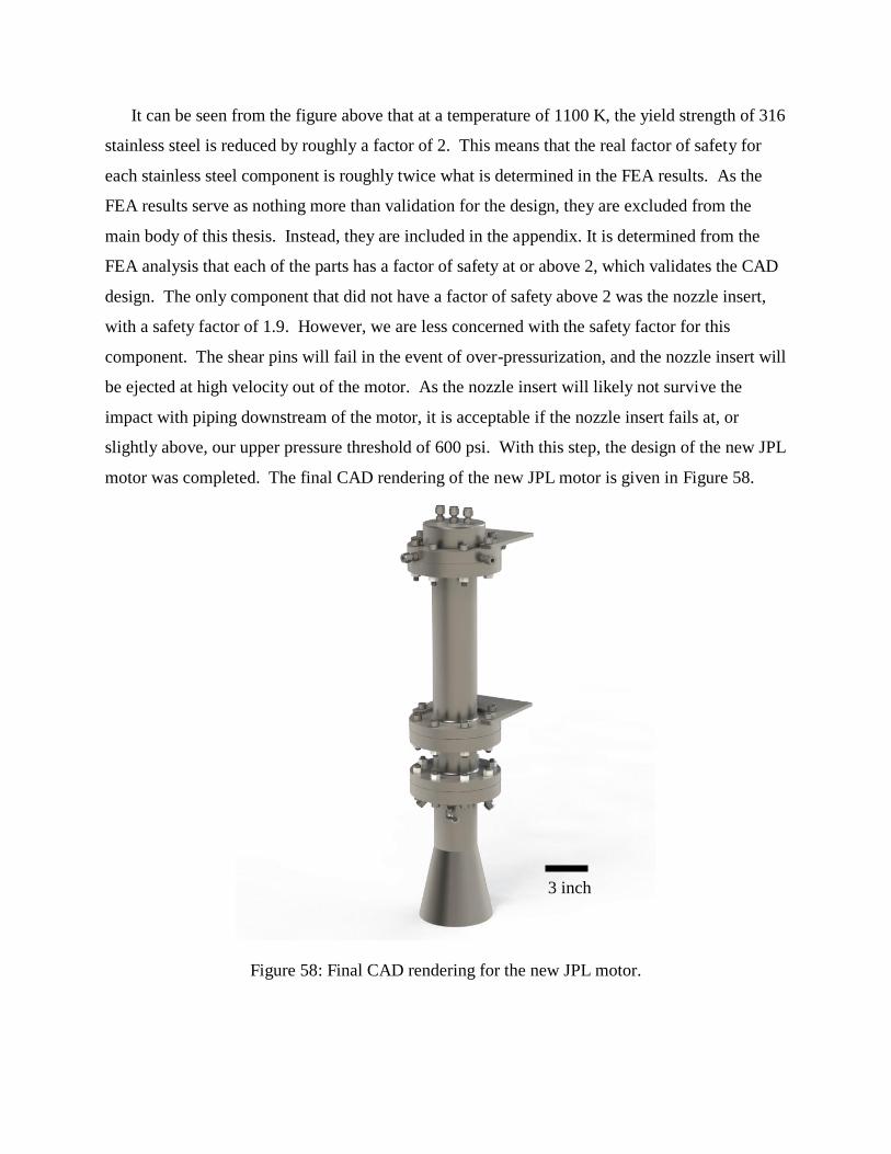
It can be seen from the figure above that at a temperature of 1100 K, the yield strength of 316
stainless steel is reduced by roughly a factor of 2. This means that the real factor of safety for
each stainless steel component is roughly twice what is determined in the FEA results. As the
FEA results serve as nothing more than validation for the design, they are excluded from the
main body of this thesis. Instead, they are included in the appendix. It is determined from the
FEA analysis that each of the parts has a factor of safety at or above 2, which validates the CAD
design. The only component that did not have a factor of safety above 2 was the nozzle insert,
with a safety factor of 1.9. However, we are less concerned with the safety factor for this
component. The shear pins will fail in the event of over-pressurization, and the nozzle insert will
be ejected at high velocity out of the motor. As the nozzle insert will likely not survive the
impact with piping downstream of the motor, it is acceptable if the nozzle insert fails at, or
slightly above, our upper pressure threshold of 600 psi. With this step, the design of the new JPL
motor was completed. The final CAD rendering of the new JPL motor is given in Figure 58.
Figure 58: Final CAD rendering for the new JPL motor.
3 inch

6 CONCLUSIONS
A comprehensive overview of ejector performance is compiled early in the thesis,
detailing the operation of both single-stage and two-stage ejectors. This overview serves as a
general reference which can be used in troubleshooting, as well as for future development.
A sensitivity analysis was performed to determine the motive/suction flow parameters
which were most influential on the performance of the single-stage ejector. Through this
sensitivity analysis, we determined that suction temperature was the most influential parameter
for ejector performance under real-world rocket engine testing conditions. It was also
determined that both the motive and suction heat capacity ratio had the smallest effect on ejector
performance.
The new model proposed in this thesis was validated using experimental characterization
data collected for the single-stage ejector. The validated model was then shown to be capable of
predict the approximate performance of the single-stage ejector during the testing of an Aerotech
F50-9T solid rocket motor within the altitude chamber. The new model was calibrated using
experimental characterization data for the two-stage ejector, and was used to predict the
performance of the two-stage ejector during the testing of a 90 Newton rocket engine at 54,000
ft. Through these experimental tests, the new model was proven to reliably predict the
performance of both the single-stage and two-stage ejector systems under real rocket engine
testing conditions.
A simple GUI was also created to provide a layer of abstraction between the underlying
model and the end user. This GUI can be used by potential customers to determine the testing
capabilities of the altitude chamber. The customer can determine what maximum simulated
altitude is possible for the testing of their rocket engine within the altitude chamber. Similarly,
the GUI can be used to determine the upper thrust limit for a given simulated altitude. This GUI
provides flexibility to the end user, streamlining the process of collaboration between academia
and industry.
A new rocket engine is also designed to characterize a hybrid grain configuration within
the altitude chamber at reduced pressure, which serves as a continuation of the atmospheric
testing campaign performed in collaboration with the Jet Propulsion Laboratory (JPL). The
major steps of the design process are discussed, culminating in the final design of the motor.

This thesis provides a strong foundational modeling which can be used to support current
and future work at the altitude facility of Zucrow Labs. The new model can also be used to
inform the future path of the altitude facility and guide the development of new testing
capabilities.

7 FUTURE WORK
In the future, the new model proposed within this thesis could be integrated into the two-
stage ejector VI to allow for automated control of each stage of the ejector system. This
automation would allow for instantaneous adjustment of the motive flow conditions to ensure
that the ambient pressure within the altitude chamber remains absolutely constant over the course
of a rocket engine test. This increase in testing control would act to increase the accuracy of
future experimental testing results while simultaneously optimizing the performance of the two-
stage ejector system. This automated control of the two-stage ejector system using the new
model could also allow for the characterization of the full thrust-profile of a rocket engine.
Similarly, this automated control could allow for the testing of a full flight profile at relevant
atmospheric conditions. In this way, the altitude facility would be able to test the full thrust and
altitude profile associated with a given mission.
The new model could be further improved by accounting for flow processes currently
absorbed by the corrective coefficient. A parallel study of the ejector system using
Computational Fluid Dynamics (CFD) would help to better inform the flow processes occurring
within the ejector, yielding a more complete model. This updated model would benefit from an
extension of the predictive capabilities to different ejector geometries. As the needs of the
altitude facility shift over time, this updated model could be used to inform future ejector designs
which provide improved thrust and simulated altitude capabilities.
With respect to the future needs of the altitude facility, the new model could also be used
to determine the theoretical performance capabilities of the two-stage ejector configured in
parallel, rather than series. This parallel configuration would allow for the altitude facility to
support the testing of higher thrust motors at lower simulated altitudes. This new testing
capability could potentially be relevant for the optimization of air-breathing propulsion systems,
leading to increased collaboration between academia and industry. The model could also be
used to predict the performance benefit of adding a third stage to the ejector system. The
addition of a third ejector in series would allow for truly representative testing of medium-thrust
rocket engines for deep space applications.
Though a preliminary theoretical sensitivity analysis was performed to determine the
impact of different motive and suction flow parameters, it would be useful to experimentally test

motive fluids with different properties. This experimental data would inform the new model,
allowing us to determine candidate fluids which could be used to further increase the
performance of the two-stage ejector system. These new candidate fluids would serve to
determine priorities regarding future facility development at ZL3.

REFERENCES
[1] R. Manikanda Kumaran, K. Vivekanand, T. Sundararajan, S. Balasubramanian, and D. Raja
Manohar, “Analysis of Diffuser and Ejector Performance in a High Altitude Test
Facility,” in 45th AIAA/ASME/SAE/ASEE Joint Propulsion Conference &
Exhibit, Denver, Colorado, 2009.
[2] F. Kong and H. D. Kim, “Optimization study of a two-stage ejector–diffuser system,”
International Journal of Heat and Mass Transfer, vol. 101, pp. 1151–1162, Oct.
2016.
[3] K. Chunnanond and S. Aphornratana, “Ejectors: applications in refrigeration technology,”
Renewable and Sustainable Energy Reviews, vol. 8, no. 2, pp. 129–155, Apr. 2004.
[4] D.-W. Sun and I. Eames, “Recent developments in the design theories and applications of
ejectors,” Journal of the Institute of Energy, vol. 68, pp. 65–79, Jun. 1995.
[5] S. Ghorbanian and S. J. Nejad, “Ejector Modeling and Examining of Possibility of
Replacing Liquid Vacuum Pump in Vacuum Production Systems,” International
Journal of Chemical Engineering and Applications, pp. 91–97, 2011.
[6] J. Liu, L. Wang, and L. Jia, “A predictive model for the performance of the ejector in
refrigeration system,” Energy Conversion and Management, vol. 150, pp. 269–276,
Oct. 2017.
[7] J. R. Lines, “Understanding ejector systems necessary to troubleshoot vacuum distillation,”
Oil and Gas Journal, vol. 97, no. 7, pp. 40–45, 1999.
[8] R. K. McGovern, K. V. Bulusu, and M. A. Antar, “One-dimensional Model of an Optimal
Ejector and Parametric Study of Ejector Efficiency,” p. 12.
[9] J. Sarkar, “Ejector enhanced vapor compression refrigeration and heat pump systems—A
review,” Renewable and Sustainable Energy Reviews, vol. 16, no. 9, pp. 6647–6659,
Dec. 2012.
[10] M. R. Kumaran, V. P. Kumaresan, T. Sundararajan, K. K., and R. D. Manohar,
“Optimization of Second Throat Ejectors for High-Altitude Test Facility,” Journal of
Propulsion and Power, vol. 25, no. 3, pp. 697–706, May 2009.
[11] Graham Corporation, Ejector - Steam Jet Ejectors - Well Operating. .
[12] J. T. Munday and D. F. Bagster, “A New Ejector Theory Applied to Steam Jet
Refrigeration,” Industrial & Engineering Chemistry Process Design and
Development, vol. 16, no. 4, pp. 442–449, Oct. 1977.

[13] J. Yan, N. Wen, L. Wang, X. Li, Z. Liu, and S. Li, “Optimization on ejector key geometries
of a two-stage ejector-based multi-evaporator refrigeration system,” Energy
Conversion and Management, vol. 175, pp. 142–150, Nov. 2018.
[14] Y. Li and Y. Wen, “The Energy-saving Analysis of Steam Ejector in plant Steam System,”
in 2010 Asia-Pacific Power and Energy Engineering Conference, 2010, pp. 1–4.
[15] N. Bilir and H. K. Ersoy, “Performance improvement of the vapour compression
refrigeration cycle by a two-phase constant area ejector,” International Journal of
Energy Research, vol. 33, no. 5, pp. 469–480, 2009.
[16] F. L. Li, B. Cao, and Q. Tian, “Analysis of Ejector Performance Using 1-D Model,”
Applied Mechanics and Materials, vol. 253–255, pp. 781–785, Dec. 2012.
[17] T. Benjamin, “Eductor pumps: The calculations,” World Pumps, vol. 2001, pp. 34–38, Jan.
2001.
[18] F. D. Berkeley, “Ejectors,” Graham Company Batavia, New York, p. 6, 1958.
[19] C. Liao and F. R. Best, “Comprehensive Gas Ejector Model,” Journal of Thermophysics
and Heat Transfer, vol. 24, no. 3, pp. 516–523, Jul. 2010.
[20] Y. Zhu, W. Cai, C. Wen, and Y. Li, “Simplified ejector model for control and
optimization,” Energy Conversion and Management, vol. 49, no. 6, pp. 1424–1432,
Jun. 2008.
[21] C. K. Drummond, “A Model for Prediction of STOVL Ejector Dynamics,” p. 14.
[22] J. H. Keenan and E. P. Neumann, “A Simple Air Ejector,” Journal of Applied Mechanics,
vol. 9, pp. A75–A81, 1942.
[23] J. H. Keenan, E. P. Neumann, and F. Lustwerk, “An Investigation of Ejector Design by
Analysis and Experiment,” Journal of Applied Mechanics, vol. ASME 17, pp. 299–
309, 1950.
[24] I. Mcgregor, “The vapour-screen method of flow visualization,” Journal of Fluid
Mechanics, vol. 11, no. 4, pp. 481–511, Dec. 1961.
[25] J. Fabri and R. Siestrunck, Advances in Applied Mechanics. Academic Press, 1958.
[26] B. J. Huang, J. M. Chang, C. P. Wang, and V. A. Petrenko, “A 1-D analysis of ejector
performance,” International Journal of Refrigeration, vol. 22, no. 5, pp. 354–364,
Aug. 1999.
[27] Y. Zhu, W. Cai, C. Wen, and Y. Li, “Shock circle model for ejector performance
evaluation,” Energy Conversion and Management, vol. 48, no. 9, pp. 2533–2541,
Sep. 2007.
[28] K. R. Hedges and P. G. Hill, “Compressible Flow Ejectors: Part I—Development of a
Finite-Difference Flow Model,” Journal of Fluids Engineering, vol. 96, no. 3, p. 272,
1974.
[29] K. Banasiak and A. Hafner, “1D Computational model of a two-phase R744 ejector for
expansion work recovery,” International Journal of Thermal Sciences, vol. 50, no.
11, pp. 2235–2247, Nov. 2011.
[30] M. Haida, M. Palacz, J. Smolka, A. J. Nowak, A. Hafner, and K. Banasiak, “A modified
homogeneous relaxation model for CO2 two-phase flow in vapour ejector,” Journal
of Physics: Conference Series, vol. 745, p. 032159, Sep. 2016.
[31] R. C. Bauer, R. C. German, and J. H. Panesci, “Methods for determining the performance
of ejector-diffuser systems.,” Journal of Spacecraft and Rockets, vol. 3, no. 2, pp.
193–200, Feb. 1966.
[32] J. Coker, “ThrustCurve Hobby Rocket Motor Simulator Data Search,” 2008. [Online].
Available: http://www.thrustcurve.org/simfilesearch.jsp?id=701. [Accessed: 10-Jul-
2019].
[33] A. Yetman, “A COMPARATIVE STUDY OF PUMPING SYSTEMS FOR A CHEMICAL
PROPULSION ALTITUDE TEST STAND.” Goddard Space Flight Center, 1966.
[34] A. C. Wright, “USAF Propellant Handbooks. Nitric Acid/Nitrogen Tetroxide Oxidizers.
Volume II.,” MARTIN MARIETTA AEROSPACE DENVER CO, Feb. 1977.
[35] A. Benhidjeb-Carayon, J. Gabl, and T. L. Pourpoint, “Hypergolic Ignition and Relights of a
Paraffin-based Hybrid Grain,” in 2018 Joint Propulsion Conference, 0 vols.,
American Institute of Aeronautics and Astronautics, 2018.
[36] J. J. Zipay, C. T. Modlin, and C. E. Larsen, “The Ultimate Factor of Safety for Aircraft and
Spacecraft - Its History, Applications and Misconceptions,” in 57th
AIAA/ASCE/AHS/ASC Structures, Structural Dynamics, and Materials Conference,
San Diego, California, USA, 2016.
[37] Parker O-Ring Handbook; ORD 5700. Cleveland, OH: Parker Hannafin Corporation, 2018.
[38] P. Karditsas and M.-J. Baptiste, “Austenitic Stainless Steel (316),” www-ferp.ecsd.edu.
[Online]. Available: http://www-ferp.ucsd.edu/LIB/PROPS/PANOS/ss.html.
[Accessed: 10-Jul-2019].

104
APPENDIX A. MATLAB CODES
EJECTOR_CEA_RUNNER.M:
function [output] = ejector_cea_runner(cea)
addpath('CEA_MATLAB', '-end');
% CEA_ROCKET_EXAMPLE: Example file for the MATLAB CEA wrapper. For in-depth
% documentation read the headers of cea_rocket_run.m,
% cea_rocket_run_single.m, and cea_rocket_read.m
% Change this variable to true to rerun CEA instead of using saved values
CEA_RUN = true;
CEA_SAVE_FILE = 'cea.mat';
Ru = 8.314;
% The CEA MATLAB code takes a MATLAB map (called a dictionary in Python or
% hash in C) as input. The dictionary uses MATLAB character arrays as the
% keys, and the value data type varies by which key is used. Details of
% each key are listed in cea_rocket_run.m
% For example: inp('key') = value.
inp = containers.Map;
inp('type') = cea.run_type; % Sets the type of CEA calculation
inp('p') = cea.Pc; % Chamber pressure
inp('p_unit') = cea.P_c_unit; % Chamber pressure units
inp('o/f') = cea.o_f; % Mixture ratio
inp('sup') = cea.AR_sup; % Supersonic area ratios
inp('fuel') = cea.fuel_name; % Fuel name from thermo.inp
inp('fuel_t') = cea.T_fuel; % Fuel inlet temperature
inp('fuel_t_unit') = cea.T_fuel_unit;
inp('ox') = cea.ox_name; % Ox name from thermo.inpj
inp('ox_t') = cea.T_ox; % Ox inlet temperature
inp('ox_t_unit') = cea.T_ox_unit;
% inp('file_name') = 'H2O2_T.inp'; % Input/output file name
if CEA_RUN
data = cea_rocket_run(inp); % Call the CEA MATLAB code
save(CEA_SAVE_FILE, 'data');
else
load(CEA_SAVE_FILE);
end

105
% The output data structure, called 'data' in this case, is also a MATLAB
% map. 'data' contains a single entry for each of the CEA calculation types
% listed ('eq' and 'fr'). For instance, if only 'fr' is listed, then 'data'
% will only contain a single entry under data('fr').
if strcmp(cea.run_type,'eq') == 1
data = data('eq');
elseif strcmp(cea.run_type,'fr') == 1
data = data('fr');
else
errormsg('Error: /n CEA Type must be one of the following: /n eq, fr');
end
% Use keys(data_eq) or keys(data_fr) to see the contents of each map
% respectively. Every output of CEA is contained in these keys, including
% molar concentrations. Most keys contain a 3D array with columns
% corresponding to the pressure, O/F, and area/pressure ratio inputs
% respectively. If only a single value is given for one of these inputs,
% the output will still be a 3D array. The squeeze() MATLAB function must
% be used to reduce the number of dimensions appropriately. Read the notes
% at the top of cea_rocket_read.m for more details.
% keys(data)
% Pulling out all results needed for the model
cp = squeeze(data('cp'));
output.Cp = cp(2);
gamma = squeeze(data('gammas'));
output.gamma = gamma(2);
t = squeeze(data('t'));
output.T = t(2);
isp = squeeze(data('isp'));
output.Isp = isp(2);
output.MW = (output.gamma*Ru)/(output.Cp*(output.gamma-1));
end
NEW_MODEL.M:
function eo = new_model(ei)
% This is the new model introduced in thesis. This 1-D model uses
% isentropic relations, compressible gas dynamics, conservation of
% momentum, and conservation of energy to determine the flow conditions
% relevant for a single stage of an ejector system. This model is only used
% for a constant-pressure ejector. The calculation architecture is
% summarized in thesis defense presentation for reference.

106
R_u = 8.314; % [J/(mol*K)]
% Compressible Gas Dynamics: Motive Mass Flow [kg/s]
eo.mdot_p = (ei.P_p0)*(ei.A_t)*...
sqrt(((ei.gamma_p/ei.R_p)*((2/(ei.gamma_p+1))^...
((ei.gamma_p+1)/(ei.gamma_p-1))))*(ei.n_p)/(ei.T_p0));
%VALUES FOR EXIT PLANE OF NOZZLE (p1)
% Isentropic Relation: Motive Nozzle Exit Static Pressure [Pa]
eo.P_p1 = ei.P_p0*((1+((ei.gamma_p-1)/2)*(ei.M_p1^2))^...
((-ei.gamma_p)/(ei.gamma_p-1)));
% Isentropic Relation: Motive Nozzle Exit Static Temperature [K]
eo.T_p1 = (ei.T_p0)*(1+((ei.gamma_p-1)/2)*(ei.M_p1^2))^(-1);
% Conditional introduced where either motive or suction gas accelerates
% isentropically to meet equal pressure mixing criteria. Two options:
% 1) Motive nozzle exit static pressure higher than suction stagnation
% pressure
% 2) Suction stagnation pressure higher than motive nozzle exit static
% pressure
if eo.P_p1 > ei.P_s0
% Mach Number of Motive Flow at Contracting Section Inlet
eo.M_p2 = sqrt(((2)/(ei.gamma_p-1))*...
((((eo.P_p1/ei.P_s0)^((ei.gamma_p-1)/(ei.gamma_p)))*...
(1+(((ei.gamma_p-1)/(2))*((ei.M_p1)^2))))-1));
% Static Temperature of Motive Flow at Contracting Section Inlet [K]
eo.T_p2 = ei.T_p0*(1+(ei.gamma_p-1)/2*eo.M_p2^2)^-1;
% Static Pressure of Motive Flow at Contracting Section Inlet [Pa]
eo.P_p2 = ei.P_s0;
% Mach Number of Suction Flow at Contracting Section Inlet
eo.M_s2 = 0;
% Static Temperature of Suction Flow at Contracting Section Inlet [K]
eo.T_s2 = ei.T_s0;
% Static Pressure of Suction Flow at Contracting Section Inlet [Pa]
eo.P_s2 = ei.P_s0;
else
% Mach Number of Motive Flow at Contracting Section Inlet
eo.M_p2 = ei.M_p1;
% Static Temperature of Motive Flow at Contracting Section Inlet [K]
eo.T_p2 = eo.T_p1;
% Static Pressure of Motive Flow at Contracting Section Inlet [Pa]
eo.P_p2 = eo.P_p1;

107
% Mach Number of Suction Flow at Contracting Section Inlet
eo.M_s2 = sqrt(((2)/(ei.gamma_s-1))*...
((((ei.P_s0/eo.P_p1)^((ei.gamma_s-1)/(ei.gamma_s)))*...
(1+(((ei.gamma_s-1)/(2))*((0)^2))))-1));
% Static Temperature of Suction Flow at Contracting Section Inlet [K]
eo.T_s2 = (ei.T_s0)*((1+((ei.gamma_s-1)/2)*...
(eo.M_s2^2))^(-1));
% Static Pressure of Suction Flow at Contracting Section Inlet [Pa]
eo.P_s2 = eo.P_p1;
end
% Isentropic relation: Expansion of Motive Plume in Mixing Chamber of
% Ejector [m^2]
eo.A_p2 = (ei.A_p1)*(ei.M_p1/eo.M_p2)*...
(2/(ei.gamma_p+1)*(1+(ei.gamma_p-1)/2*eo.M_p2^2))^((ei.gamma_p+1)/(2*(ei.gamma_p-
1)))/...
(2/(ei.gamma_p+1)*(1+(ei.gamma_p-1)/2*ei.M_p1^2))^((ei.gamma_p+1)/(2*(ei.gamma_p-
1)));
% Calculation of Suction Area [m^2]
eo.A_s2 = ei.A_c - eo.A_p2;
eo.A_mix = ei.A_3;
% Equal Pressure Mixing Assumption [Pa]
eo.P_mix = eo.P_s2;
% Mass Flow Averaged Heat Capacity [J/K]
eo.Cp_mix = (eo.mdot_p*ei.Cp_p+ei.mdot_s*ei.Cp_s)/(eo.mdot_p+ei.mdot_s);
% Calculation of Entrainment Ratio
eo.er = ei.mdot_s/eo.mdot_p;
% Mixed Mass Flow [kg/s]
eo.mdot_mix = eo.mdot_p + ei.mdot_s;
% Mixed Gamma from Comprehensive Ejector Model
eo.gamma_mix = ((ei.gamma_p/(ei.gamma_p-1))+...
(ei.gamma_s/(ei.gamma_s-1))*(ei.R_s/ei.R_p)*eo.er)/...
((1/(ei.gamma_p-1))+(1/(ei.gamma_s-1))*(ei.R_s/ei.R_p)*eo.er);
% Mass Flow Averaged Molecular Weight [kg/mol]
eo.MW_mix = (eo.mdot_p*ei.MW_p+ei.mdot_s*ei.MW_s)/(eo.mdot_p+ei.mdot_s);
eo.R_mix = R_u/eo.MW_mix;

108
% Conservation of momentum: Mach Number of Mixed Flow
eo.M_mix =
sqrt(((ei.n_m*eo.A_p2)/(eo.gamma_mix*eo.A_mix))*(1+ei.gamma_p*eo.M_p2^2)+...
((eo.A_s2*ei.n_m)/(eo.gamma_mix*eo.A_mix))*(1+ei.gamma_s*eo.M_s2^2)-
1/eo.gamma_mix);
% Conservation of Energy: Static Temperature of Mixed Flow [K]
eo.T_mix = (1/(eo.mdot_mix*(eo.Cp_mix+0.5*eo.M_mix^2*eo.gamma_mix*eo.R_mix)))*...
(eo.mdot_p*ei.Cp_p*eo.T_p2+0.5*eo.mdot_p*eo.M_p2^2*ei.gamma_p*ei.R_p*eo.T_p2+...
ei.mdot_s*ei.Cp_s*eo.T_s2+0.5*eo.mdot_p*eo.M_s2^2*ei.gamma_s*ei.R_s*eo.T_s2);
% Shock occurs if Mach Number of Mixed Flow is greater than 1.
if eo.M_mix > 1
% Normal Shock Theory: Static Pressure of Mixed Flow After Normal Shock [Pa]
eo.P_3 = (eo.P_mix)*(1+((2*eo.gamma_mix)/(eo.gamma_mix+1))*...
((eo.M_mix^2)-1));
% Normal Shock Theory: Mach Number of Mixed Flow After Normal Shock
eo.M_3 = sqrt((1+((eo.gamma_mix-1)/2)*(eo.M_mix^2))/((eo.gamma_mix)*...
(eo.M_mix^2)-((eo.gamma_mix-1)/2)));
else
% Static Pressure of Mixed Flow without Normal Shock [Pa]
eo.P_3 = eo.P_mix;
% Mach Number of Mixed FLow without Normal Shock
eo.M_3 = eo.M_mix;
end
% Isentropic Relation: Stagnation Pressure of Mixed Flow [Pa]
eo.P_e = real((eo.P_3)*((1+((eo.gamma_mix-1)/2)*(eo.M_3^2))^...
((eo.gamma_mix)/(eo.gamma_mix-1))));
end
SINGLE_STAGE_EJECTOR_SENSITIVITY_ANALYSIS.M:
% This script is used to determine the response of entrainment ratio to
% changes in model input conditions. For this treatment, each of the input
% value is given some nominal value. There is also a 10% higher and 10%
% lower value for each of the input values. The script then scans over the
% full range of potential suction mass flow rates to determine the maximum
% suction mass flow rate which still satisfies the constant area and exit
% pressure constraints. The suction stagnation pressure is held constant
% for this treatment. The final sensitivity graph is created using
% excel.
% Constant Section Diameter Constraint Value [m]

109
D3_req = 2.15*0.0254;
% Motive Nozzle Throat Diameter [m]
Dt = 0.495*0.0254;
% Motive Nozzle Throat Area [m^2]
At = pi/4*((Dt)^2);
% Motive Nozzle Exit Diameter [m]
De = 1.16*0.0254;
% Motive Nozzle Exit Area [m^2]
Ae = pi/4*((De)^2);
% Motive Nozzle Expansion Ratio
eps = Ae/At;
% Gas coefficients
ox_a = 28.186;
ox_b = 6.3011;
ox_c = -0.74986;
ox_d = 0;
n2_a = 27.336;
n2_b = 6.23;
n2_c = -0.95082;
n2_d = 0;
% Efficiencies modified based on design point of single-stage ejector
n_p = 0.993;
n_s = 0.96;
phi_p = 0.9;
phi_m = 0.955;
%% MOTIVE FLOW PARAMETERS
% Motive Stagnation Pressure [Pa]
P_p0 = 214*6894.76;
% Motive Stagnation Temperature [F]
T_p0_F = 500;
% Motive Stagnation Temperature [K]
T_p0 = (T_p0_F-32).*5./9+273.15;
% Motive Stagnation Temperature Vector [K]
T_p0_vector = (([T_p0_F*0.9,T_p0_F,T_p0_F*1.1])-32).*5./9+273.15;
% Motive Heat Capacity Ratio
gamma_p = 1.4;
% Motive Heat Capacity Ratio Vector
gamma_p_vector = [gamma_p*0.9,gamma_p,gamma_p*1.1];
% Motive Molecular Weight [kg/mol]
MW_p = 0.02884;
% Motive Molecular Weight [kg/mol]

110
MW_p_vector = [MW_p*0.9,MW_p,MW_p*1.1];
% Motive Heat Capacity [J/(kg*K)]
Cp_p = (0.79*((n2_a)+(n2_b*(T_p0/1000))+...
(n2_c*((T_p0/1000)^2))+(n2_d*((T_p0/1000)^3)))+...
0.21*((ox_a)+(ox_b*(T_p0/1000))+(ox_c*((T_p0/1000)^2))+...
(ox_d*((T_p0/1000)^3))))/(MW_p);
% Motive Heat Capacity Vector [J/(kg*K)]
Cp_p_vector = [Cp_p*0.9,Cp_p,Cp_p*1.1];
% Motive Heat Capacity Vector from Temperature Variance [J/(kg*K)]
Cp_p_T_p0_vector = (0.79.*((n2_a)+(n2_b.*(T_p0_vector./1000))+...
(n2_c.*((T_p0_vector./1000).^2))+(n2_d.*((T_p0_vector./1000).^3)))+...
0.21.*((ox_a)+(ox_b.*(T_p0_vector./1000))+(ox_c.*((T_p0_vector./1000).^2))+...
(ox_d.*((T_p0_vector./1000).^3))))./(MW_p);
% Motive Heat Capacity Vector from Molecular Weight Variance [J/(kg*K)]
Cp_p_MW_p_vector = (0.79.*((n2_a)+(n2_b.*(T_p0./1000))+...
(n2_c.*((T_p0./1000).^2))+(n2_d.*((T_p0./1000).^3)))+...
0.21.*((ox_a)+(ox_b.*(T_p0./1000))+(ox_c.*((T_p0./1000).^2))+...
(ox_d.*((T_p0./1000).^3))))./(MW_p_vector);
% Vector of Motive Nozzle Exit Mach Numbers from Heat Capacity Ratio
% Variance
M_p1_vector = zeros(1,length(gamma_p_vector));
for i = 1:length(gamma_p_vector)
M_p1_vector(i) = Mach_finder(eps,gamma_p_vector(i),5);
end
%% SUCTION FLOW PARAMETERS
% Suction Stagnation Temperature [F]
T_s0_F = 500;
% Suction Stagnation Temperature [K]
T_s0 = (T_s0_F-32).*5./9+273.15;
% Suction Stagnation Temperature Vector [K]
T_s0_vector = (([T_s0_F*0.9,T_s0_F,T_s0_F*1.1])-32).*5./9+273.15;
% Suction Molecular Weight [kg/mol]
MW_s = 0.028;
% Suction Molecular Weight Vector [kg/mol]
MW_s_vector = [MW_s*0.9,MW_s,MW_s*1.1];
% Suction Heat Capacity Ratio
gamma_s = 1.4;
% Suction Heat Capacity Ratio Vector
gamma_s_vector = [gamma_s*0.9,gamma_s,gamma_s*1.1];
% Suction Heat Capacity Ratio [J/(kg*K)]
Cp_s = ((n2_a)+(n2_b*(T_s0/1000))+...
(n2_c*((T_s0./1000)^2))+(n2_d*((T_s0/1000)^3)))/(MW_s);
% Suction Heat Capacity Ratio Vector [J/(kg*K)]

111
Cp_s_vector = [Cp_s*0.9,Cp_s,Cp_s*1.1];
% Suction Heat Capacity Ratio Vector from Temperature Variance [J/(kg*K)]
Cp_s_T_s0_vector = ((n2_a)+(n2_b.*(T_s0_vector./1000))+...
(n2_c.*((T_s0_vector./1000).^2))+(n2_d.*((T_s0_vector./1000).^3)))./(MW_s);
% Suction Heat Capacity Ratio Vector from Molecular Weight Variance [J/(kg*K)]
Cp_s_MW_s_vector = ((n2_a)+(n2_b.*(T_s0./1000))+...
(n2_c.*((T_s0./1000).^2))+(n2_d.*((T_s0./1000).^3)))./(MW_s_vector);
% Suction Stagnation Pressure [Pa]
P_s0 = 5*6894.76;
%% LOOPING STRUCTURE
% Matrix Used to Store all Input Value Combinations
sensitivity_matrix = zeros(13,9);
% Defining the Different Input Value Combinations
sensitivity_matrix(1,:) = [T_p0_vector(1),gamma_p_vector(2),MW_p_vector(2),...
Cp_p_T_p0_vector(1),M_p1_vector(2),T_s0_vector(2),MW_s_vector(2),...
gamma_s_vector(2),Cp_s_vector(2)];
sensitivity_matrix(2,:) = [T_p0_vector(3),gamma_p_vector(2),MW_p_vector(2),...
Cp_p_T_p0_vector(3),M_p1_vector(2),T_s0_vector(2),MW_s_vector(2),...
gamma_s_vector(2),Cp_s_vector(2)];
sensitivity_matrix(3,:) = [T_p0_vector(2),gamma_p_vector(1),MW_p_vector(2),...
Cp_p_vector(2),M_p1_vector(1),T_s0_vector(2),MW_s_vector(2),...
gamma_s_vector(2),Cp_s_vector(2)];
sensitivity_matrix(4,:) = [T_p0_vector(2),gamma_p_vector(3),MW_p_vector(2),...
Cp_p_vector(2),M_p1_vector(3),T_s0_vector(2),MW_s_vector(2),...
gamma_s_vector(2),Cp_s_vector(2)];
sensitivity_matrix(5,:) = [T_p0_vector(2),gamma_p_vector(2),MW_p_vector(1),...
Cp_p_MW_p_vector(1),M_p1_vector(2),T_s0_vector(2),MW_s_vector(2),...
gamma_s_vector(2),Cp_s_vector(2)];
sensitivity_matrix(6,:) = [T_p0_vector(2),gamma_p_vector(2),MW_p_vector(3),...
Cp_p_MW_p_vector(3),M_p1_vector(2),T_s0_vector(2),MW_s_vector(2),...
gamma_s_vector(2),Cp_s_vector(2)];
sensitivity_matrix(7,:) = [T_p0_vector(2),gamma_p_vector(2),MW_p_vector(2),...
Cp_p_vector(2),M_p1_vector(2),T_s0_vector(1),MW_s_vector(2),...
gamma_s_vector(2),Cp_s_T_s0_vector(1)];
sensitivity_matrix(8,:) = [T_p0_vector(2),gamma_p_vector(2),MW_p_vector(2),...
Cp_p_vector(2),M_p1_vector(2),T_s0_vector(3),MW_s_vector(2),...

112
gamma_s_vector(2),Cp_s_T_s0_vector(3)];
sensitivity_matrix(9,:) = [T_p0_vector(2),gamma_p_vector(2),MW_p_vector(2),...
Cp_p_vector(2),M_p1_vector(2),T_s0_vector(2),MW_s_vector(1),...
gamma_s_vector(2),Cp_s_MW_s_vector(1)];
sensitivity_matrix(10,:) = [T_p0_vector(2),gamma_p_vector(2),MW_p_vector(2),...
Cp_p_vector(2),M_p1_vector(2),T_s0_vector(2),MW_s_vector(3),...
gamma_s_vector(2),Cp_s_MW_s_vector(3)];
sensitivity_matrix(11,:) = [T_p0_vector(2),gamma_p_vector(2),MW_p_vector(2),...
Cp_p_vector(2),M_p1_vector(2),T_s0_vector(2),MW_s_vector(2),...
gamma_s_vector(1),Cp_s_vector(2)];
sensitivity_matrix(12,:) = [T_p0_vector(2),gamma_p_vector(2),MW_p_vector(2),...
Cp_p_vector(2),M_p1_vector(2),T_s0_vector(2),MW_s_vector(2),...
gamma_s_vector(3),Cp_s_vector(2)];
% Nominal Case Used to Compare Against Varied Test Cases
sensitivity_matrix(13,:) = [T_p0_vector(2),gamma_p_vector(2),MW_p_vector(2),...
Cp_p_vector(2 ),M_p1_vector(2),T_s0_vector(2),MW_s_vector(2),...
gamma_s_vector(2),Cp_s_vector(2)];
er_pass_vector = zeros(1,size(sensitivity_matrix,1));
% Going Through all of the Different Input Value Combinations
for j_3 = 1:size(sensitivity_matrix,1)
% Loading in Relevant Input Values for this Combination Set
sens_T_p0 = sensitivity_matrix(j_3,1);
sens_gamma_p = sensitivity_matrix(j_3,2);
sens_MW_p = sensitivity_matrix(j_3,3);
sens_Cp_p = sensitivity_matrix(j_3,4);
sens_M_p1 = sensitivity_matrix(j_3,5);
sens_T_s0 = sensitivity_matrix(j_3,6);
sens_MW_s = sensitivity_matrix(j_3,7);
sens_gamma_s = sensitivity_matrix(j_3,8);
sens_Cp_s = sensitivity_matrix(j_3,9);
% Defining Range of Potential Suction Mass Flow Rates [kg/s]
mdot_s_vector = 0.0001:0.0001:0.7;
% Defining Arbitrarily High Exit Pressure
P_e_pass = 50*101325;
mdot_s_pass = 0;

113
% Scanning Over Range of Potential Suction Mass Flow Rates
for j_2 = 1:size(mdot_s_vector,2)
% Loading in Current Suction Mass Flow Rate Being Evaluated
mdot_s = mdot_s_vector(j_2);
% Running the Huang Model
[P_e,D_3,mdot_p] =...
onedimensionalsolver...
(At,Ae,sens_T_p0,P_p0,sens_Cp_p,sens_MW_p,sens_gamma_p,mdot_s,...
sens_T_s0,P_s0,sens_Cp_s,sens_MW_s,sens_gamma_s,n_p,n_s,phi_p,phi_m,sens_M_p1);
% Successful Run Must Satisfy Both Area and Pressure Requirement
if (D_3 <= D3_req - 0.005 || D_3 >= D3_req + 0.005) || (P_e < 101325)
P_e = 0;
else
% This conditional is used to find the maximum suction mass
% flow rate which still satisfies the above constraints
if mdot_s > mdot_s_pass
P_e_pass = P_e;
mdot_s_pass = mdot_s;
end
end
end
% Saves the maximum suction mass flow rate, and thus entrainment ratio
er_pass_vector(j_3) = mdot_s_pass/mdot_p;
end
t = 1:13;
plot(t,er_pass_vector);
% figure(1)
% plot(motive_pressure_vector_psi, er_vector)
% title('Entrainment Ratio vs Motive Pressure');
% ylabel('Entrainment Ratio');
% xlabel('Motive Pressure (psi)');
% legend('T_{s0} = 70 F','T_{s0} = 500 F','T_{s0} = 1000 F','T_{s0} = 1500 F');
% hold on
%
% figure(2)
% plot(motive_pressure_vector_psi, mdot_s_vector_lbs)
% title('Suction Flow Rate vs Motive Pressure');

114
% ylabel('Suction Flow Rate (lbm/s)');
% xlabel('Motive Pressure (psi)');
% legend('T_{s0} = 70 F','T_{s0} = 500 F','T_{s0} = 1000 F','T_{s0} = 1500 F');
% hold on
SINGLE_STAGE_EJECTOR_SENSITIVITY_ANALYSIS_RW.M:
% This script is used to determine the response of entrainment ratio to
% changes in model input conditions. For this treatment, each of the input
% value is given some nominal value. The high and low input values are
% defined relative to what we expect - or could expect - during a rocket
% test. The script then scans over the full range of potential
% suction mass flow rates to determine the maximum suction mass flow rate
% which still satisfies the constant area and exit pressure constraints.
% The final sensitivity graph is created using excel.
% Constant Section Diameter Constraint Value [m]
D3_req = 2.15*0.0254;
% Motive Nozzle Throat Diameter [m]
Dt = 0.495*0.0254;
% Motive Nozzle Throat Area [m^2]
At = pi/4*((Dt)^2);
% Motive Nozzle Exit Diameter [m]
De = 1.16*0.0254;
% Motive Nozzle Exit Area [m^2]
Ae = pi/4*((De)^2);
% Motive Nozzle Expansion Ratio
eps = Ae/At;
% Gas coefficients
ox_a = 28.186;
ox_b = 6.3011;
ox_c = -0.74986;
ox_d = 0;
n2_a = 27.336;
n2_b = 6.23;
n2_c = -0.95082;
n2_d = 0;
% Efficiencies modified based on design point of single-stage ejector
n_p = 0.993;
n_s = 0.96;
phi_p = 0.9;
phi_m = 0.955;

115
%% MOTIVE FLOW PARAMETERS
% Motive Stagnation Pressure [Pa]
P_p0 = 214*6894.76;
% Motive Stagnation Temperature [K]
T_p0 = 477; % K
% Motive Stagnation Temperature Vector [K]
T_p0_vector = [298,477,700];
% Motive Heat Capacity Ratio
gamma_p = 1.4;
% Motive Heat Capacity Ratio Vector
gamma_p_vector = [1.28,1.4,1.67];
% Motive Molecular Weight [kg/mol]
MW_p = 0.02884; % kg/mol
% Motive Molecular Weight [kg/mol]
MW_p_vector = [0.018,0.02884,0.039];
% Motive Heat Capacity [J/(kg*K)]
Cp_p = (0.79*((n2_a)+(n2_b*(T_p0/1000))+...
(n2_c*((T_p0/1000)^2))+(n2_d*((T_p0/1000)^3)))+...
0.21*((ox_a)+(ox_b*(T_p0/1000))+(ox_c*((T_p0/1000)^2))+...
(ox_d*((T_p0/1000)^3))))/(MW_p); % J/kg-K
% Motive Heat Capacity Vector [J/(kg*K)]
Cp_p_vector = [Cp_p*0.9,Cp_p,Cp_p*1.1];
% Motive Heat Capacity Vector from Temperature Variance [J/(kg*K)]
Cp_p_T_p0_vector = (0.79.*((n2_a)+(n2_b.*(T_p0_vector./1000))+...
(n2_c.*((T_p0_vector./1000).^2))+(n2_d.*((T_p0_vector./1000).^3)))+...
0.21.*((ox_a)+(ox_b.*(T_p0_vector./1000))+(ox_c.*((T_p0_vector./1000).^2))+...
(ox_d.*((T_p0_vector./1000).^3))))./(MW_p); % J/kg-K
% Motive Heat Capacity Vector from Molecular Weight Variance [J/(kg*K)]
Cp_p_MW_p_vector = (0.79.*((n2_a)+(n2_b.*(T_p0./1000))+...
(n2_c.*((T_p0./1000).^2))+(n2_d.*((T_p0./1000).^3)))+...
0.21.*((ox_a)+(ox_b.*(T_p0./1000))+(ox_c.*((T_p0./1000).^2))+...
(ox_d.*((T_p0./1000).^3))))./(MW_p_vector); % J/kg-K
M_p1_vector = zeros(1,length(gamma_p_vector));
for i = 1:length(gamma_p_vector)
M_p1_vector(i) = Mach_finder(eps,gamma_p_vector(i),5);
end
%% SUCTION FLOW PARAMETERS
% Suction Stagnation Temperature [K]
T_s0 = 1000; % K
% Suction Stagnation Temperature Vector [K]
T_s0_vector = [298,1000,2500]; % K

116
% Suction Molecular Weight [kg/mol]
MW_s = 0.02;
% Suction Molecular Weight Vector [kg/mol]
MW_s_vector = [0.010,0.020,0.028];
% Suction Heat Capacity Ratio
gamma_s = 1.3;
% Suction Heat Capacity Ratio Vector
gamma_s_vector = [1.19,1.3,1.4];
% Suction Heat Capacity Ratio [J/(kg*K)]
Cp_s = ((n2_a)+(n2_b*(T_s0/1000))+...
(n2_c*((T_s0./1000)^2))+(n2_d*((T_s0/1000)^3)))/(MW_s); % J/kg-K
% Suction Heat Capacity Ratio Vector [J/(kg*K)]
Cp_s_vector = [Cp_s*0.9,Cp_s,Cp_s*1.1];
% Suction Heat Capacity Ratio Vector from Temperature Variance [J/(kg*K)]
Cp_s_T_s0_vector = ((n2_a)+(n2_b.*(T_s0_vector./1000))+...
(n2_c.*((T_s0_vector./1000).^2))+(n2_d.*((T_s0_vector./1000).^3)))./(MW_s); % J/kg-K
% Suction Heat Capacity Ratio Vector from Molecular Weight Variance [J/(kg*K)]
Cp_s_MW_s_vector = ((n2_a)+(n2_b.*(T_s0./1000))+...
(n2_c.*((T_s0./1000).^2))+(n2_d.*((T_s0./1000).^3)))./(MW_s_vector); % J/kg-K
% Suction Stagnation Pressure [Pa]
P_s0 = 5*6894.76; % Pa
%% LOOPING STRUCTURE
% Matrix Used to Store all Input Value Combinations
sensitivity_matrix = zeros(13,9);
% Defining the Different Input Value Combinations
sensitivity_matrix(1,:) = [T_p0_vector(1),gamma_p_vector(2),MW_p_vector(2),...
Cp_p_T_p0_vector(1),M_p1_vector(2),T_s0_vector(2),MW_s_vector(2),...
gamma_s_vector(2),Cp_s_vector(2)];
sensitivity_matrix(2,:) = [T_p0_vector(3),gamma_p_vector(2),MW_p_vector(2),...
Cp_p_T_p0_vector(3),M_p1_vector(2),T_s0_vector(2),MW_s_vector(2),...
gamma_s_vector(2),Cp_s_vector(2)];
sensitivity_matrix(3,:) = [T_p0_vector(2),gamma_p_vector(1),MW_p_vector(2),...
Cp_p_vector(2),M_p1_vector(1),T_s0_vector(2),MW_s_vector(2),...
gamma_s_vector(2),Cp_s_vector(2)];
sensitivity_matrix(4,:) = [T_p0_vector(2),gamma_p_vector(3),MW_p_vector(2),...
Cp_p_vector(2),M_p1_vector(3),T_s0_vector(2),MW_s_vector(2),...
gamma_s_vector(2),Cp_s_vector(2)];
sensitivity_matrix(5,:) = [T_p0_vector(2),gamma_p_vector(2),MW_p_vector(1),...
Cp_p_MW_p_vector(1),M_p1_vector(2),T_s0_vector(2),MW_s_vector(2),...

117
gamma_s_vector(2),Cp_s_vector(2)];
sensitivity_matrix(6,:) = [T_p0_vector(2),gamma_p_vector(2),MW_p_vector(3),...
Cp_p_MW_p_vector(3),M_p1_vector(2),T_s0_vector(2),MW_s_vector(2),...
gamma_s_vector(2),Cp_s_vector(2)];
sensitivity_matrix(7,:) = [T_p0_vector(2),gamma_p_vector(2),MW_p_vector(2),...
Cp_p_vector(2),M_p1_vector(2),T_s0_vector(1),MW_s_vector(2),...
gamma_s_vector(2),Cp_s_T_s0_vector(1)];
sensitivity_matrix(8,:) = [T_p0_vector(2),gamma_p_vector(2),MW_p_vector(2),...
Cp_p_vector(2),M_p1_vector(2),T_s0_vector(3),MW_s_vector(2),...
gamma_s_vector(2),Cp_s_T_s0_vector(3)];
sensitivity_matrix(9,:) = [T_p0_vector(2),gamma_p_vector(2),MW_p_vector(2),...
Cp_p_vector(2),M_p1_vector(2),T_s0_vector(2),MW_s_vector(1),...
gamma_s_vector(2),Cp_s_MW_s_vector(1)];
sensitivity_matrix(10,:) = [T_p0_vector(2),gamma_p_vector(2),MW_p_vector(2),...
Cp_p_vector(2),M_p1_vector(2),T_s0_vector(2),MW_s_vector(3),...
gamma_s_vector(2),Cp_s_MW_s_vector(3)];
sensitivity_matrix(11,:) = [T_p0_vector(2),gamma_p_vector(2),MW_p_vector(2),...
Cp_p_vector(2),M_p1_vector(2),T_s0_vector(2),MW_s_vector(2),...
gamma_s_vector(1),Cp_s_vector(2)];
sensitivity_matrix(12,:) = [T_p0_vector(2),gamma_p_vector(2),MW_p_vector(2),...
Cp_p_vector(2),M_p1_vector(2),T_s0_vector(2),MW_s_vector(2),...
gamma_s_vector(3),Cp_s_vector(2)];
% Nominal Case Used to Compare Against Varied Test Cases
sensitivity_matrix(13,:) = [T_p0_vector(2),gamma_p_vector(2),MW_p_vector(2),...
Cp_p_vector(2),M_p1_vector(2),T_s0_vector(2),MW_s_vector(2),...
gamma_s_vector(2),Cp_s_vector(2)];
er_pass_vector = zeros(1,size(sensitivity_matrix,1));
% Going Through all of the Different Input Value Combinations
for j_3 = 1:size(sensitivity_matrix,1)
% Loading in Relevant Input Values for this Combination Set
sens_T_p0 = sensitivity_matrix(j_3,1);
sens_gamma_p = sensitivity_matrix(j_3,2);
sens_MW_p = sensitivity_matrix(j_3,3);
sens_Cp_p = sensitivity_matrix(j_3,4);
sens_M_p1 = sensitivity_matrix(j_3,5);

118
sens_T_s0 = sensitivity_matrix(j_3,6);
sens_MW_s = sensitivity_matrix(j_3,7);
sens_gamma_s = sensitivity_matrix(j_3,8);
sens_Cp_s = sensitivity_matrix(j_3,9);
% Defining Range of Potential Suction Mass Flow Rates [kg/s]
mdot_s_vector = 0.0001:0.0001:0.7; %kg/s
% Defining Arbitrarily High Exit Pressure
P_e_pass = 50*101325;
mdot_s_pass = 0;
% Scanning Over Range of Potential Suction Mass Flow Rates
for j_2 = 1:size(mdot_s_vector,2)
% Loading in Current Suction Mass Flow Rate Being Evaluated
mdot_s = mdot_s_vector(j_2);
% Running the Huang Model
[P_e,D_3,mdot_p] =...
onedimensionalsolver...
(At,Ae,sens_T_p0,P_p0,sens_Cp_p,sens_MW_p,sens_gamma_p,mdot_s,...
sens_T_s0,P_s0,sens_Cp_s,sens_MW_s,sens_gamma_s,n_p,n_s,phi_p,phi_m,sens_M_p1);
% Successful Run Must Satisfy Both Area and Pressure Requirement
if (D_3 <= D3_req - 0.005 || D_3 >= D3_req + 0.005) || (P_e < 101325)
P_e = 0;
else
% This conditional is used to find the maximum suction mass
% flow rate which still satisfies the above constraints
if mdot_s > mdot_s_pass
P_e_pass = P_e;
mdot_s_pass = mdot_s;
end
end
end
% Saves the maximum suction mass flow rate, and thus entrainment ratio
er_pass_vector(j_3) = mdot_s_pass/mdot_p;
end
t = 1:13;
plot(t,er_pass_vector);

119
% figure(1)
% plot(motive_pressure_vector_psi, er_vector)
% title('Entrainment Ratio vs Motive Pressure');
% ylabel('Entrainment Ratio');
% xlabel('Motive Pressure (psi)');
% legend('T_{s0} = 70 F','T_{s0} = 500 F','T_{s0} = 1000 F','T_{s0} = 1500 F');
% hold on
%
% figure(2)
% plot(motive_pressure_vector_psi, mdot_s_vector_lbs)
% title('Suction Flow Rate vs Motive Pressure');
% ylabel('Suction Flow Rate (lbm/s)');
% xlabel('Motive Pressure (psi)');
% legend('T_{s0} = 70 F','T_{s0} = 500 F','T_{s0} = 1000 F','T_{s0} = 1500 F');
% hold on
SINGLE_STAGE_EJECTOR_SENSITIVITY_ANALYSIS_RW_ALT.M:
% This script is used to determine the response of simulated altitude to
% changes in model input conditions. For this treatment, each of the input
% value is given some nominal value. The high and low input values are
% defined relative to what we expect - or could expect - during a rocket
% test. The script then scans over the full range of potential
% suction stagnation pressures to determine the minimum suction stagnation
% pressure which still satisfies the constant area and exit pressure
% constraints. The final sensitivity graph is created using excel.
% Constant Section Diameter Constraint Value [m]
D3_req = 2.15*0.0254;
% Motive Nozzle Throat Diameter [m]
Dt = 0.495*0.0254;
% Motive Nozzle Throat Area [m^2]
At = pi/4*((Dt)^2);
% Motive Nozzle Exit Diameter [m]
De = 1.16*0.0254;
% Motive Nozzle Exit Area [m^2]
Ae = pi/4*((De)^2);
% Motive Nozzle Expansion Ratio
eps = Ae/At;
% Gas coefficients
ox_a = 28.186;
ox_b = 6.3011;
ox_c = -0.74986;
ox_d = 0;
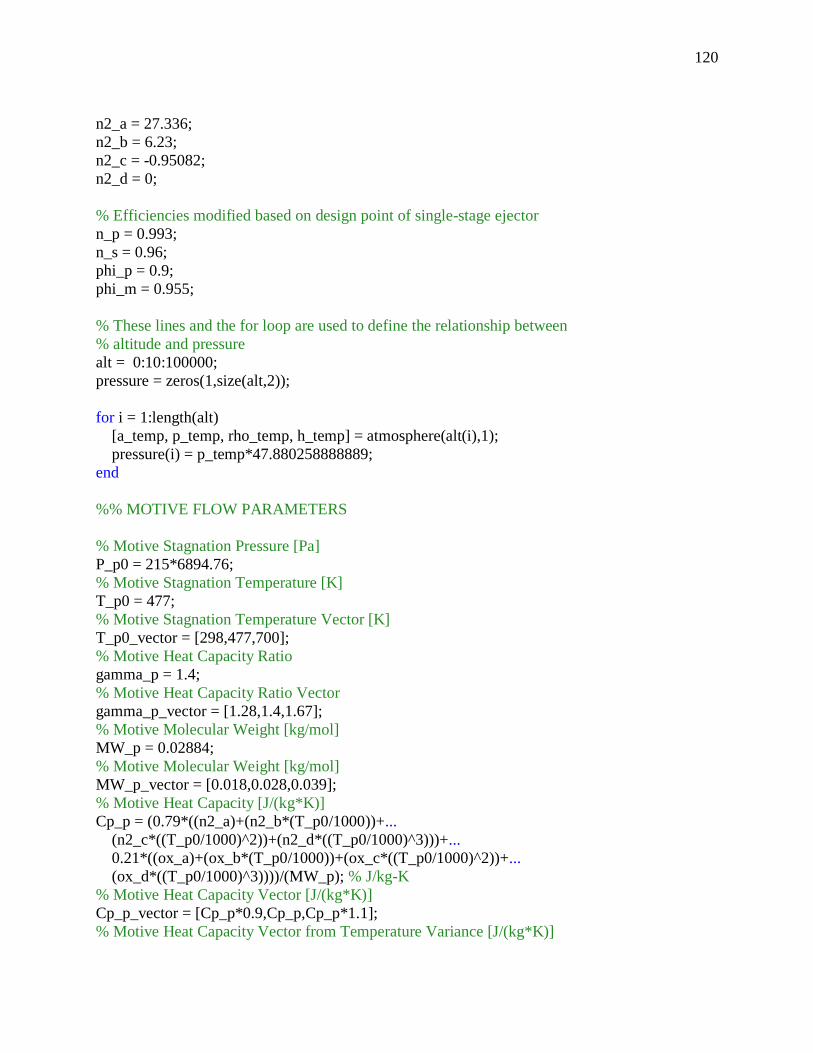
120
n2_a = 27.336;
n2_b = 6.23;
n2_c = -0.95082;
n2_d = 0;
% Efficiencies modified based on design point of single-stage ejector
n_p = 0.993;
n_s = 0.96;
phi_p = 0.9;
phi_m = 0.955;
% These lines and the for loop are used to define the relationship between
% altitude and pressure
alt = 0:10:100000;
pressure = zeros(1,size(alt,2));
for i = 1:length(alt)
[a_temp, p_temp, rho_temp, h_temp] = atmosphere(alt(i),1);
pressure(i) = p_temp*47.880258888889;
end
%% MOTIVE FLOW PARAMETERS
% Motive Stagnation Pressure [Pa]
P_p0 = 215*6894.76;
% Motive Stagnation Temperature [K]
T_p0 = 477;
% Motive Stagnation Temperature Vector [K]
T_p0_vector = [298,477,700];
% Motive Heat Capacity Ratio
gamma_p = 1.4;
% Motive Heat Capacity Ratio Vector
gamma_p_vector = [1.28,1.4,1.67];
% Motive Molecular Weight [kg/mol]
MW_p = 0.02884;
% Motive Molecular Weight [kg/mol]
MW_p_vector = [0.018,0.028,0.039];
% Motive Heat Capacity [J/(kg*K)]
Cp_p = (0.79*((n2_a)+(n2_b*(T_p0/1000))+...
(n2_c*((T_p0/1000)^2))+(n2_d*((T_p0/1000)^3)))+...
0.21*((ox_a)+(ox_b*(T_p0/1000))+(ox_c*((T_p0/1000)^2))+...
(ox_d*((T_p0/1000)^3))))/(MW_p); % J/kg-K
% Motive Heat Capacity Vector [J/(kg*K)]
Cp_p_vector = [Cp_p*0.9,Cp_p,Cp_p*1.1];
% Motive Heat Capacity Vector from Temperature Variance [J/(kg*K)]

121
Cp_p_T_p0_vector = (0.79.*((n2_a)+(n2_b.*(T_p0_vector./1000))+...
(n2_c.*((T_p0_vector./1000).^2))+(n2_d.*((T_p0_vector./1000).^3)))+...
0.21.*((ox_a)+(ox_b.*(T_p0_vector./1000))+(ox_c.*((T_p0_vector./1000).^2))+...
(ox_d.*((T_p0_vector./1000).^3))))./(MW_p); % J/kg-K
% Motive Heat Capacity Vector from Molecular Weight Variance [J/(kg*K)]
Cp_p_MW_p_vector = (0.79.*((n2_a)+(n2_b.*(T_p0./1000))+...
(n2_c.*((T_p0./1000).^2))+(n2_d.*((T_p0./1000).^3)))+...
0.21.*((ox_a)+(ox_b.*(T_p0./1000))+(ox_c.*((T_p0./1000).^2))+...
(ox_d.*((T_p0./1000).^3))))./(MW_p_vector); % J/kg-K
% Vector of Motive Nozzle Exit Mach Numbers from Heat Capacity Ratio
% Variance
M_p1_vector = zeros(1,length(gamma_p_vector));
for i = 1:length(gamma_p_vector)
M_p1_vector(i) = Mach_finder(eps,gamma_p_vector(i),5);
end
%% SUCTION FLOW PARAMETERS
% Suction Stagnation Temperature [K]
T_s0 = 1644;
% Suction Stagnation Temperature Vector [K]
T_s0_vector = [298,1644,2500];
% Suction Molecular Weight [kg/mol]
MW_s = 0.02;
% Suction Molecular Weight Vector [kg/mol]
MW_s_vector = [0.010,0.020,0.028];
% Suction Heat Capacity Ratio
gamma_s = 1.3;
% Suction Heat Capacity Ratio Vector
gamma_s_vector = [1.19,1.3,1.4];
% Suction Heat Capacity Ratio [J/(kg*K)]
Cp_s = ((n2_a)+(n2_b*(T_s0/1000))+...
(n2_c*((T_s0./1000)^2))+(n2_d*((T_s0/1000)^3)))/(MW_s);
% Suction Heat Capacity Ratio Vector [J/(kg*K)]
Cp_s_vector = [Cp_s*0.9,Cp_s,Cp_s*1.1];
% Suction Heat Capacity Ratio Vector from Temperature Variance [J/(kg*K)]
Cp_s_T_s0_vector = ((n2_a)+(n2_b.*(T_s0_vector./1000))+...
(n2_c.*((T_s0_vector./1000).^2))+(n2_d.*((T_s0_vector./1000).^3)))./(MW_s);
% Suction Heat Capacity Ratio Vector from Molecular Weight Variance [J/(kg*K)]
Cp_s_MW_s_vector = ((n2_a)+(n2_b.*(T_s0./1000))+...
(n2_c.*((T_s0./1000).^2))+(n2_d.*((T_s0./1000).^3)))./(MW_s_vector);
% Suction Mass Flow Rate [kg/s]
mdot_s = 0.033;
%% LOOPING STRUCTURE

122
% Matrix Used to Store all Input Value Combinations
sensitivity_matrix = zeros(13,9);
% Defining the Different Input Value Combinations
sensitivity_matrix(1,:) = [T_p0_vector(1),gamma_p_vector(2),MW_p_vector(2),...
Cp_p_T_p0_vector(1),M_p1_vector(2),T_s0_vector(2),MW_s_vector(2),...
gamma_s_vector(2),Cp_s_vector(2)];
sensitivity_matrix(2,:) = [T_p0_vector(3),gamma_p_vector(2),MW_p_vector(2),...
Cp_p_T_p0_vector(3),M_p1_vector(2),T_s0_vector(2),MW_s_vector(2),...
gamma_s_vector(2),Cp_s_vector(2)];
sensitivity_matrix(3,:) = [T_p0_vector(2),gamma_p_vector(1),MW_p_vector(2),...
Cp_p_vector(2),M_p1_vector(1),T_s0_vector(2),MW_s_vector(2),...
gamma_s_vector(2),Cp_s_vector(2)];
sensitivity_matrix(4,:) = [T_p0_vector(2),gamma_p_vector(3),MW_p_vector(2),...
Cp_p_vector(2),M_p1_vector(3),T_s0_vector(2),MW_s_vector(2),...
gamma_s_vector(2),Cp_s_vector(2)];
sensitivity_matrix(5,:) = [T_p0_vector(2),gamma_p_vector(2),MW_p_vector(1),...
Cp_p_MW_p_vector(1),M_p1_vector(2),T_s0_vector(2),MW_s_vector(2),...
gamma_s_vector(2),Cp_s_vector(2)];
sensitivity_matrix(6,:) = [T_p0_vector(2),gamma_p_vector(2),MW_p_vector(3),...
Cp_p_MW_p_vector(3),M_p1_vector(2),T_s0_vector(2),MW_s_vector(2),...
gamma_s_vector(2),Cp_s_vector(2)];
sensitivity_matrix(7,:) = [T_p0_vector(2),gamma_p_vector(2),MW_p_vector(2),...
Cp_p_vector(2),M_p1_vector(2),T_s0_vector(1),MW_s_vector(2),...
gamma_s_vector(2),Cp_s_T_s0_vector(1)];
sensitivity_matrix(8,:) = [T_p0_vector(2),gamma_p_vector(2),MW_p_vector(2),...
Cp_p_vector(2),M_p1_vector(2),T_s0_vector(3),MW_s_vector(2),...
gamma_s_vector(2),Cp_s_T_s0_vector(3)];
sensitivity_matrix(9,:) = [T_p0_vector(2),gamma_p_vector(2),MW_p_vector(2),...
Cp_p_vector(2),M_p1_vector(2),T_s0_vector(2),MW_s_vector(1),...
gamma_s_vector(2),Cp_s_MW_s_vector(1)];
sensitivity_matrix(10,:) = [T_p0_vector(2),gamma_p_vector(2),MW_p_vector(2),...
Cp_p_vector(2),M_p1_vector(2),T_s0_vector(2),MW_s_vector(3),...
gamma_s_vector(2),Cp_s_MW_s_vector(3)];
sensitivity_matrix(11,:) = [T_p0_vector(2),gamma_p_vector(2),MW_p_vector(2),...

123
Cp_p_vector(2),M_p1_vector(2),T_s0_vector(2),MW_s_vector(2),...
gamma_s_vector(1),Cp_s_vector(2)];
sensitivity_matrix(12,:) = [T_p0_vector(2),gamma_p_vector(2),MW_p_vector(2),...
Cp_p_vector(2),M_p1_vector(2),T_s0_vector(2),MW_s_vector(2),...
gamma_s_vector(3),Cp_s_vector(2)];
% Nominal Case Used to Compare Against Varied Test Cases
sensitivity_matrix(13,:) = [T_p0_vector(2),gamma_p_vector(2),MW_p_vector(2),...
Cp_p_vector(2),M_p1_vector(2),T_s0_vector(2),MW_s_vector(2),...
gamma_s_vector(2),Cp_s_vector(2)];
P_s0_pass_vector = zeros(1,size(sensitivity_matrix,1));
% Going Through all of the Different Input Value Combinations
for j_3 = 1:size(sensitivity_matrix,1)
% Loading in Relevant Input Values for this Combination Set
sens_T_p0 = sensitivity_matrix(j_3,1);
sens_gamma_p = sensitivity_matrix(j_3,2);
sens_MW_p = sensitivity_matrix(j_3,3);
sens_Cp_p = sensitivity_matrix(j_3,4);
sens_M_p1 = sensitivity_matrix(j_3,5);
sens_T_s0 = sensitivity_matrix(j_3,6);
sens_MW_s = sensitivity_matrix(j_3,7);
sens_gamma_s = sensitivity_matrix(j_3,8);
sens_Cp_s = sensitivity_matrix(j_3,9);
% Defining Range of Potential Suction Stagnation Pressures [Pa]
P_s0_vector = 0.001*6894.76:0.001*6894.76:14.7*6894.76;
% Defining Arbitrarily High Exit Pressure
P_e_pass = 50*101325;
P_s0_pass = 20*6894.76;
% Scanning Over Range of Potential Suction Stagnation Pressures
for j_2 = 1:size(P_s0_vector,2)
% Loading in Current Suction Stagnation Pressure Being Evaluated
P_s0 = P_s0_vector(j_2);
% Running the Huang Model
[P_e,D_3,mdot_p] =...
onedimensionalsolver...
(At,Ae,sens_T_p0,P_p0,sens_Cp_p,sens_MW_p,sens_gamma_p,mdot_s,...
124
sens_T_s0,P_s0,sens_Cp_s,sens_MW_s,sens_gamma_s,n_p,n_s,phi_p,phi_m,sens_M_p1);
% Successful Run Must Satisfy Both Area and Pressure Requirement
if (D_3 <= D3_req - 0.005 || D_3 >= D3_req + 0.005) || (P_e < 101325)
P_e = 0;
else
% This conditional is used to find the maximum suction mass
% flow rate which still satisfies the above constraints
if P_s0 < P_s0_pass
P_e_pass = P_e;
P_s0_pass = P_s0;
end
end
end
% Saves the minimum suction stagnation pressure
P_s0_pass_vector(j_3) = P_s0_pass;
end
% Converting minimum suction stagnation pressures to equivalent simulated
% altitudes
alt_pass_vector = zeros(1,length(P_s0_pass_vector));
for i = 1:length(P_s0_pass_vector)
P_s0_temp = P_s0_pass_vector(i);
[~,index] = min(abs(pressure-P_s0_temp));
alt_pass_vector(i) = alt(index);
end
t = 1:13;
figure(1)
hold on
plot(pressure./6894.76,alt);
scatter(P_s0_pass_vector./6894.76,alt_pass_vector);
hold off
% figure(1)
% plot(motive_pressure_vector_psi, er_vector)
% title('Entrainment Ratio vs Motive Pressure');
% ylabel('Entrainment Ratio');
% xlabel('Motive Pressure (psi)');
% legend('T_{s0} = 70 F','T_{s0} = 500 F','T_{s0} = 1000 F','T_{s0} = 1500 F');
% hold on
%

125
% figure(2)
% plot(motive_pressure_vector_psi, mdot_s_vector_lbs)
% title('Suction Flow Rate vs Motive Pressure');
% ylabel('Suction Flow Rate (lbm/s)');
% xlabel('Motive Pressure (psi)');
% legend('T_{s0} = 70 F','T_{s0} = 500 F','T_{s0} = 1000 F','T_{s0} = 1500 F');
% hold on
TEST_DATA_ANALYSIS_ SINGLE_STAGE_EJECTOR_4_5_EXP.M:
% This script is used to load experimental characterization data for the
% single-stage ejector with low expansion ratio nozzle. The new 1-D model
% is then used to determine the momentum coefficient value that satisfies
% each of the experimentally defined data points. The results momentum
% coefficient curve is then shown graphically. Must have curve-fitting
% toolbox to run this script.
% Loading Data from Single-Stage Ejector Performance Characterization
test_data = xlsread('VE_4_5_Test_Results.xlsx',1,'A2:D196');
% Motive Stagnation Pressure [Pa]
P_p0_vector = ((test_data(:,1)).').*6894.75729;
% Suction Mass Flow Rate [kg/s]
mdot_s_vector = ((test_data(:,4)).')./2.20462262;
% Suction Stagnation Pressure [Pa]
P_s0_vector = ((test_data(:,2)).').*6894.75729;
% Mixing Chamber Static Pressure [Pa]
P_mc_vector = ((test_data(:,3)).').*6894.75729;
%Typical isentropic efficiency for CD nozzle
n_p = 0.993;
% Initializing Momentum Coefficient Scanning Range
n_m_vector = 0.001:0.001:1;
%DEFINING GEOMETRY VALUES AND CONSTANT VALUES
% Constant Section Diameter [m]
D_3 = 2.15*0.0254;
% Constant Section Area [m^2]
A_3 = (pi)/(4)*((D_3)^2);
% Motive Nozzle Throat Diameter [m]
D_t = 0.495*0.0254;
% Motive Nozzle Throat Area [m^2]
A_t = pi/4*((D_t)^2);
% Motive Nozzle Exit Diameter [m]
D_p1 = 1.16*0.0254;

126
% Motive NOzzle Exit Area [m^2]
A_p1 = pi/4*((D_p1)^2);
% Motive Nozzle Expansion Ratio
eps = A_p1/A_t;
% Contraction Section Diameter [m]
D_c = 4*0.0254;
% Contraction Section Area [m^2]
A_c = pi/4*((D_c)^2);
% Coefficients Used for Heat Capacity Calaculation
a_ox = 28.186;
b_ox = 6.3011;
c_ox = -0.74986;
d_ox = 0;
% Coefficients Used for Heat Capacity Calculation
a_n2 = 27.336;
b_n2 = 6.23;
c_n2 = -0.95082;
d_n2 = 0;
% Universal Gas Constant [J/(K*mol)]
R_u = 8.314;
%% DEFINING MOTIVE FLOW VALUES
% Motive Stagnation Temperature [K]
T_p0 = 298;
% Motive Heat Capacity Ratio
gamma_p = 1.4;
% Motive Molecular Weight [kg/mol]
MW_p = 0.029;
% Motive Heat Capacity [J/K]
Cp_p = (0.79*((a_n2)+(b_n2*(T_p0/1000))+...
(c_n2*((T_p0/1000)^2))+(d_n2*((T_p0/1000)^3)))+...
0.21*((a_ox)+(b_ox*(T_p0/1000))+(c_ox*((T_p0/1000)^2))+...
(d_ox*((T_p0/1000)^3))))/(MW_p);
% Mach Number at Motive Nozzle Exit Plane
M_p1 = Mach_finder(eps,gamma_p,5);
% Motive Specific Gas Constant [J/(kg*K)]
R_p = R_u/MW_p;
%% DEFINING ENTRAINED FLOW VALUES
% Suction Stagnation Temperature [K]
T_s0 = 298;

127
% Suction Molecular Weight [kg/mol]
MW_s = 0.028;
% Suction Heat Capacity Ratio
gamma_s = 1.4;
% Suction Heat Capacity [J/K]
Cp_s = ((a_n2)+...
(b_n2*(T_s0/1000))+...
(c_n2*((T_s0/1000)^2))+...
(d_n2*((T_s0/1000)^3)))/...
(MW_s);
% Suction Specific Gas Constant [J/(kg*K)]
R_s = R_u/MW_s;
%% RUNNING THE CODE
% These vectors are defined so that only the experimental data points which
% yield a momentum coefficient between 0 and 1 are reflected in the fit.
success_n_m_vector = [];
success_P_exit_vector = zeros(1,length(P_p0_vector));
successful_run_index = [];
% Outer loop scans over all of the experimental data points
for j_2 = 1:length(P_p0_vector)
% Current best values. Exit pressure is main constraint, so initially
% set to some arbitrarily high value.
current_success_n_m = 0;
current_success_mdot = 0;
current_success_P_e = 101325*50;
% Loading in values corresponding to current experimental data point
P_p0 = P_p0_vector(j_2);
P_s0 = P_s0_vector(j_2);
mdot_s = mdot_s_vector(j_2);
% Scanning over range of possible momentum coefficient value
for j_1 = 1:length(n_m_vector)
% Loading in current momentum coefficient value
n_m = n_m_vector(j_1);
% Loading all constant model input values into a struct
ei.A_t = A_t;
ei.T_p0 = T_p0;
ei.P_p0 = P_p0;
ei.Cp_p = Cp_p;
128
ei.MW_p = MW_p;
ei.gamma_p = gamma_p;
ei.mdot_s = mdot_s;
ei.T_s0 = T_s0;
ei.P_s0 = P_s0;
ei.Cp_s = Cp_s;
ei.MW_s = MW_s;
ei.gamma_s = gamma_s;
ei.n_p = n_p;
ei.M_p1 = M_p1;
ei.R_p = R_p;
ei.R_s = R_s;
ei.A_3 = A_3;
ei.n_m = n_m;
ei.A_p1 = A_p1;
ei.A_c = A_c;
% Running model
eo = new_model(ei);
% Exit pressure must be higher than ambient (14.7 psia) for a run
% to be successful
if eo.P_e < 101325
eo.P_e = 0;
D_3 = 0;
eo.mdot_p = 0;
end
% Choosing momentum coefficient value which yields exit pressure
% JUST above ambient pressure
if eo.P_e ~= 0
if eo.P_e < current_success_P_e
current_success_n_m = n_m;
current_success_P_e = eo.P_e;
end
end
end
if current_success_P_e < 101325*50
success_n_m_vector(j_2) = current_success_n_m;
success_P_exit_vector(j_2) = current_success_P_e;
successful_run_index = [successful_run_index, j_2];
end
end
%% DEFINING ALL VALUES FOR FITTING AND GRAPHING

129
stg1_P_p0_vector_graph = P_p0_vector(successful_run_index)./6894.76;
stg1_P_p1_vector_graph = stg1_P_p0_vector_graph.*((1+((gamma_p-1)/2)*(M_p1^2))^...
((-gamma_p)/(gamma_p-1)));
stg1_mdot_s_vector_graph = mdot_s_vector(successful_run_index);
success_n_m_vector_graph = success_n_m_vector(successful_run_index);
success_P_exit_vector_graph = success_P_exit_vector(successful_run_index);
stg1_P_s0_vector_graph = P_s0_vector(successful_run_index);
stg1_P_mc_vector_graph = P_mc_vector(successful_run_index);
stg1_P_ratio_vector_graph = stg1_P_p1_vector_graph./stg1_P_mc_vector_graph;
stg1_P_p0_vector_col = stg1_P_p0_vector_graph.';
stg1_mdot_s_vector_col = stg1_mdot_s_vector_graph.';
success_n_m_vector_col = success_n_m_vector_graph.';
success_P_exit_vector_col = (success_P_exit_vector_graph.')./6894.7;
stg1_P_s0_vector_col = (stg1_P_s0_vector_graph.')./6894.7;
stg1_P_mc_vector_col = (stg1_P_mc_vector_graph.')./6894.7;
stg1_P_ratio_vector_col = stg1_P_ratio_vector_graph.';
%% PLOTTING DATA ALONG WITH CURVE FITS
% Creating Fit
[nm_fit,nm_gof] = createFit(stg1_P_p0_vector_graph, mdot_s_vector,
success_n_m_vector_graph);
figure(1)
hold on
scatter3(stg1_P_p0_vector_graph,stg1_mdot_s_vector_graph,success_n_m_vector_graph);
plot(nm_fit,[stg1_P_p0_vector_col,stg1_mdot_s_vector_col],success_n_m_vector_col);
hold off
xlabel('Motive Pressure (psia)');
ylabel('Suction Mass Flow Rate (kg/s)');
zlabel('Energy Efficiency Coefficient');
set(legend,'visible','off')
zlim([0 1]);
TEST_DATA_ANALYSIS_ SINGLE_STAGE_EJECTOR_8_5_EXP.M:
% This script is used to load experimental characterization data for the
% single-stage ejector with high expansion ratio nozzle. The new 1-D model
% is then used to determine the momentum coefficient value that satisfies
% each of the experimentally defined data points. The results momentum
% coefficient curve is then shown graphically. Must have curve-fitting
% toolbox to run this script.

130
% Loading Data from Single-Stage Ejector Performance Characterization
test_data = xlsread('VE_8_5_Test_Results.xlsx',1,'A2:C178');
% Motive Stagnation Pressure [Pa]
P_p0_vector = ((test_data(:,1)).').*6894.75729;
% Suction Mass Flow Rate [kg/s]
mdot_s_vector = ((test_data(:,3)).')./2.20462262;
% Suction Stagnation Pressure [Pa]
P_s0_vector = ((test_data(:,2)).').*6894.75729;
%Typical isentropic efficiency for CD nozzle
n_p = 0.993;
% Initializing Momentum Coefficient Scanning Range
n_m_vector = 0.001:0.001:1;
%DEFINING GEOMETRY VALUES AND CONSTANT VALUES
% Constant Section Diameter [m]
D_3 = 2.15*0.0254;
% Constant Section Area [m^2]
A_3 = (pi)/(4)*((D_3)^2);
% Motive Nozzle Throat Diameter [m]
D_t = 0.495*0.0254;
% Motive Nozzle Throat Area [m^2]
A_t = pi/4*((D_t)^2);
% Motive Nozzle Exit Diameter [m]
D_p1 = 1.16*0.0254;
% Motive NOzzle Exit Area [m^2]
A_p1 = pi/4*((D_p1)^2);
% Motive Nozzle Expansion Ratio
eps = A_p1/A_t;
% Contraction Section Diameter [m]
D_c = 4*0.0254;
% Contraction Section Area [m^2]
A_c = pi/4*((D_c)^2);
% Coefficients Used for Heat Capacity Calaculation
a_ox = 28.186;
b_ox = 6.3011;
c_ox = -0.74986;
d_ox = 0;
% Coefficients Used for Heat Capacity Calculation
a_n2 = 27.336;
b_n2 = 6.23;
c_n2 = -0.95082;

131
d_n2 = 0;
% Universal Gas Constant [J/(K*mol)]
R_u = 8.314;
%% DEFINING MOTIVE FLOW VALUES
% Motive Stagnation Temperature [K]
T_p0 = 298;
% Motive Heat Capacity Ratio
gamma_p = 1.4;
% Motive Molecular Weight [kg/mol]
MW_p = 0.029;
% Motive Heat Capacity [J/K]
Cp_p = (0.79*((a_n2)+(b_n2*(T_p0/1000))+...
(c_n2*((T_p0/1000)^2))+(d_n2*((T_p0/1000)^3)))+...
0.21*((a_ox)+(b_ox*(T_p0/1000))+(c_ox*((T_p0/1000)^2))+...
(d_ox*((T_p0/1000)^3))))/(MW_p);
% Mach Number at Motive Nozzle Exit Plane
M_p1 = Mach_finder(eps,gamma_p,5);
% Motive Specific Gas Constant [J/(kg*K)]
R_p = R_u/MW_p;
%% DEFINING ENTRAINED FLOW VALUES
% Suction Stagnation Temperature [K]
T_s0 = 298;
% Suction Molecular Weight [kg/mol]
MW_s = 0.028;
% Suction Heat Capacity Ratio
gamma_s = 1.4;
% Suction Heat Capacity [J/K]
Cp_s = ((a_n2)+...
(b_n2*(T_s0/1000))+...
(c_n2*((T_s0/1000)^2))+...
(d_n2*((T_s0/1000)^3)))/...
(MW_s);
% Suction Specific Gas Constant [J/(kg*K)]
R_s = R_u/MW_s;
%% RUNNING THE CODE
% These vectors are defined so that only the experimental data points which
% yield a momentum coefficient between 0 and 1 are reflected in the fit.
success_n_m_vector = [];
success_P_exit_vector = zeros(1,length(P_p0_vector));

132
successful_run_index = [];
% Outer loop scans over all of the experimental data points
for j_2 = 1:length(P_p0_vector)
% Current best values. Exit pressure is main constraint, so initially
% set to some arbitrarily high value.
current_success_n_m = 0;
current_success_mdot = 0;
current_success_P_e = 101325*50;
% Loading in values corresponding to current experimental data point
P_p0 = P_p0_vector(j_2);
P_s0 = P_s0_vector(j_2);
mdot_s = mdot_s_vector(j_2);
% Scanning over range of possible momentum coefficient value
for j_1 = 1:length(n_m_vector)
% Loading in current momentum coefficient value
n_m = n_m_vector(j_1);
% Loading all constant model input values into a struct
ei.A_t = A_t;
ei.T_p0 = T_p0;
ei.P_p0 = P_p0;
ei.Cp_p = Cp_p;
ei.MW_p = MW_p;
ei.gamma_p = gamma_p;
ei.mdot_s = mdot_s;
ei.T_s0 = T_s0;
ei.P_s0 = P_s0;
ei.Cp_s = Cp_s;
ei.MW_s = MW_s;
ei.gamma_s = gamma_s;
ei.n_p = n_p;
ei.M_p1 = M_p1;
ei.R_p = R_p;
ei.R_s = R_s;
ei.A_3 = A_3;
ei.n_m = n_m;
ei.A_p1 = A_p1;
ei.A_c = A_c;
% Running model
eo = new_model(ei);

133
% Exit pressure must be higher than ambient (14.7 psia) for a run
% to be successful
if eo.P_e < 101325
eo.P_e = 0;
D_3 = 0;
eo.mdot_p = 0;
end
% Choosing momentum coefficient value which yields exit pressure
% JUST above ambient pressure
if eo.P_e ~= 0
if eo.P_e < current_success_P_e
current_success_n_m = n_m;
current_success_P_e = eo.P_e;
end
end
end
if current_success_P_e < 101325*50
success_n_m_vector(j_2) = current_success_n_m;
success_P_exit_vector(j_2) = current_success_P_e;
successful_run_index = [successful_run_index, j_2];
passed = passed + 1
else
failed_run_index = [failed_run_index, j_2];
failed = failed + 1
end
end
%% DEFINING ALL VALUES FOR FITTING AND GRAPHING
stg1_P_p0_vector_graph = P_p0_vector(successful_run_index)./6894.76;
stg1_P_p1_vector_graph = stg1_P_p0_vector_graph.*((1+((gamma_p-1)/2)*(M_p1^2))^...
((-gamma_p)/(gamma_p-1)));
stg1_mdot_s_vector_graph = mdot_s_vector(successful_run_index);
success_n_m_vector_graph = success_n_m_vector(successful_run_index);
success_P_exit_vector_graph = success_P_exit_vector(successful_run_index);
stg1_P_s0_vector_graph = P_s0_vector(successful_run_index);
stg1_P_p0_vector_col = stg1_P_p0_vector_graph.';
stg1_mdot_s_vector_col = stg1_mdot_s_vector_graph.';
success_n_m_vector_col = success_n_m_vector_graph.';
success_P_exit_vector_col = (success_P_exit_vector_graph.')./6894.7;
stg1_P_s0_vector_col = (stg1_P_s0_vector_graph.')./6894.7;

134
%% PLOTTING DATA ALONG WITH CURVE FITS
% Creating Fit
[nm_fit,nm_gof] = createFit(stg1_P_p0_vector_graph, mdot_s_vector,
success_n_m_vector_graph);
figure(1)
hold on
scatter3(stg1_P_p0_vector_graph,stg1_mdot_s_vector_graph,success_n_m_vector_graph);
plot(nm_fit,[stg1_P_p0_vector_col,stg1_mdot_s_vector_col],success_n_m_vector_col);
hold off
xlabel('Motive Pressure (psia)');
ylabel('Suction Mass Flow Rate (kg/s)');
zlabel('Energy Efficiency Coefficient');
set(legend,'visible','off')
zlim([0 1]);
TEST_DATA_ANALYSIS_ SINGLE_STAGE_EJECTOR_F50_MOTOR.M:
% This script is used to load experimental characterization data for the
% single-stage ejector with original nozzle during the testing of a small
% solid rocket motor within the altitude chamber. The new 1-D model is then
% used to determine the momentum coefficient value that satisfies each
% of the experimentally defined data points. The resulting momentum
% coefficient curve is then shown graphically.
%% Determining the Isp of the motor
% Defining thrust curve for F50-9T motor, taken from Aerotech website
time_step = 0.1;
f50_time_vector = 0:time_step:1.5;
f50_thrust_vector = [72,70.5,70,69.5,68,67,64,61,56.5,51.5,43,25,6,2,1,0];
f50_time_vector_col = f50_time_vector.';
f50_thrust_vector_col = f50_thrust_vector.';
plot(f50_time_vector,f50_thrust_vector);
% Creating a fit for interpolation
f50_thrust_fit = fit(f50_time_vector_col,f50_thrust_vector_col,'poly7');
plot(f50_thrust_fit,f50_time_vector_col,f50_thrust_vector_col);
% Determine Isp such that thrust and mass flow are true
Isp = 130; %s
135
total_prop_mass_available = 54.25/1000;
gravity = 9.81;
% Determining exhaust mass flow curve
f50_mass_flow_vector = f50_thrust_vector./((gravity).*(Isp));
% Validating Isp value
total_prop_mass = 0;
for integr_index = 1:size(f50_mass_flow_vector,2)-1
avg_mass_flow =
(f50_mass_flow_vector(integr_index)+f50_mass_flow_vector(integr_index+1))/2;
total_prop_mass = total_prop_mass + ((time_step)*(avg_mass_flow));
end
disp(total_prop_mass);
disp(total_prop_mass_available);
%% Determining the steady state temperature of the exhaust flow
% Determining the assymptotic temperature approach
f_50_temp_vector = [380,615,810,960,1085,1175];
f_50_temp_time_vector = [148,148.2,148.4,148.6,148.8,149];
f_50_temp_vector_col = f_50_temp_vector.';
f_50_temp_time_vector_col = f_50_temp_time_vector.';
plot(f_50_temp_time_vector,f_50_temp_vector);
f50_temp_fit = fit(f_50_temp_time_vector_col,f_50_temp_vector_col,'poly2');
x_temp_graphing_vector = 100:0.01:200;
y_temp_graphing_vector = (-500)./(x_temp_graphing_vector-147.5)+1500;
figure(1)
plot(x_temp_graphing_vector,y_temp_graphing_vector);
hold on
scatter(f_50_temp_time_vector,f_50_temp_vector);
title('Projected Temperature vs Time');
xlabel('Time (sec)');
ylabel('Temperature (k)');
xlim([146 170]);
ylim([200 1700]);
%% Code to evaluate the test firing data points

136
% Typical efficiency for CD nozzle
ei.n_p = 0.993;
% Defining full range of potential momentum coefficient values
n_m_vector = 0.001:0.001:1;
% Experimental run time
time_vector = 147.85:0.1:149.35;
%DEFINING GEOMETRY VALUES AND CONSTANT VALUES
% Constant Section Diameter [m]
D_3 = 2.15 * 0.0254;
% Constant Section Area [m^2]
ei.A_3 = (pi)/(4)*((D_3)^2);
% Motive Nozzle Throat Diameter [m]
D_t = 0.495 * 0.0254;
% Motive Nozzle Throat Area [m^2]
ei.A_t = pi/4*((D_t)^2);
% Motive Nozzle Exit Diameter [m]
D_e = 1.16*0.0254;
% Motive NOzzle Exit Area [m^2]
ei.A_p1 = pi/4*((D_e)^2);
% Motive Nozzle Expansion Ratio
eps = ei.A_p1/ei.A_t;
% Contraction Section Diameter [m]
D_c = 4*0.0254;
% Contraction Section Area [m^2]
ei.A_c = pi/4*((D_c)^2);
% Universal Gas Constant [J/(K*mol)]
R_u = 8.314;
% Coefficients Used for Heat Capacity Calaculation
a_ox = 28.186;
b_ox = 6.3011;
c_ox = -0.74986;
d_ox = 0;
a_n2 = 27.336;
b_n2 = 6.23;
c_n2 = -0.95082;
d_n2 = 0;
%DEFINING MOTIVE FLOW VALUES

137
% Motive Stagnation Temperature [K]
ei.T_p0 = 298;
% Motive Heat Capacity Ratio
ei.gamma_p = 1.4;
% Motive Molecular Weight [kg/mol]
ei.MW_p = 0.029;
% Motive Heat Capacity [J/K]
ei.Cp_p = (0.79*((a_n2)+(b_n2*(ei.T_p0/1000))+...
(c_n2*((ei.T_p0/1000)^2))+(d_n2*((ei.T_p0/1000)^3)))+...
0.21*((a_ox)+(b_ox*(ei.T_p0/1000))+(c_ox*((ei.T_p0/1000)^2))+...
(d_ox*((ei.T_p0/1000)^3))))/(ei.MW_p);
% Mach Number at Motive Nozzle Exit Plane
ei.M_p1 = Mach_finder(eps,ei.gamma_p,5);
% Motive Specific Gas Constant [J/(kg*K)]
ei.R_p = R_u/ei.MW_p;
% Defining Motive Stagnation Pressure [Pa}
P_p0_vector = (167*6894.7).*(ones(size(f50_mass_flow_vector,2)));
% Calculating Motive Mass Flow Rate [kg/s]
mdot_p = (P_p0_vector(1))*(ei.A_t)*...
sqrt(((ei.gamma_p/ei.R_p)*((2/(ei.gamma_p+1))^...
((ei.gamma_p+1)/(ei.gamma_p-1))))*(ei.n_p)/(ei.T_p0));
%DEFINING ENTRAINED FLOW VALUES
% Suction Stagnation Temperature [K]
ei.T_s0 = 1500;
% Suction Molecular Weight [kg/mol]
ei.MW_s = 0.02304;
% Suction Heat Capacity Ratio
ei.gamma_s = 1.278;
% Suction Specific Gas Constant [J/(kg*K)]
ei.R_s = R_u/ei.MW_s;
% Suction Heat Capacity [J/K]
ei.Cp_s = ((ei.gamma_s)*(ei.R_s))/(ei.gamma_s-1);
% Defining Response of Suction Stagnation Pressure During Testing
P_s0_vector_psi = [8.35,8.35,8.35,8.35,8.35,8.35,8.35,8.32,8.25,8.1,...
7.85,7.7,7.5,7.45,7.42,7.4];
P_s0_vector = P_s0_vector_psi.*6894.7;
% Converting to Equivalent Nitrogen Mass Flow Rate [kg/s]
mdot_s_vector = f50_mass_flow_vector.*(ei.T_s0./298).*(ei.MW_p./ei.MW_s);
figure(2)
yyaxis left;
plot(time_vector,f50_mass_flow_vector);
xlabel('Time (sec)');
ylabel('Entrained Mass Flow (kg/sec)');

138
title('Comparing Entrained Pressure/Mass Flow Curves F50-6T');
yyaxis right;
plot(time_vector,P_s0_vector);
ylabel('Entrained Pressure (psia)');
success_n_m_vector = zeros(1,size(f50_mass_flow_vector,2));
success_pressure_exit_vector = zeros(1,size(f50_mass_flow_vector,2));
successful_run_index = [];
% Equivalent Nitrogen Mass Flow Rate Fluid Characteristics
ei.T_s0 = ei.T_p0; %from fit of temp data
ei.MW_s = ei.MW_p; %from data sheet for grain
ei.gamma_s = ei.gamma_p; %from Data Sheet for grain
ei.R_s = R_u/ei.MW_p;
ei.Cp_s = ((ei.gamma_p)*(ei.R_p))/(ei.gamma_p-1);
% Scanning Over Range of POtential Suction Mass Flow Rate Values
for j_2 = 1:length(mdot_s_vector)
% Current best values. Exit pressure is main constraint, so initially
% set to some arbitrarily high value.
current_success_n_m = 0;
current_success_pressure_exit = 101325*50;
% Loading in values corresponding to current experimental data point
ei.P_p0 = P_p0_vector(j_2);
ei.P_s0 = P_s0_vector(j_2);
ei.mdot_s = mdot_s_vector(j_2);
% Scanning over range of possible momentum coefficient value
for j_1 = 1:size(n_m_vector,2)
% Loading in current momentum coefficient value
ei.n_m = n_m_vector(j_1);
% Running model
eo = new_model(ei);
% Exit pressure must be higher than ambient (14.7 psia) for a run
% to be successful
if eo.P_e < 101325
eo.P_e = 0;
D_3 = 0;
eo.mdot_p = 0;
end

139
% Choosing momentum coefficient value which yields exit pressure
% JUST above ambient pressure
if eo.P_e ~= 0
if eo.P_e < current_success_pressure_exit
current_success_n_m = ei.n_m;
current_success_pressure_exit = eo.P_e;
end
end
end
if current_success_pressure_exit < 101325*40
success_n_m_vector(j_2) = current_success_n_m;
success_pressure_exit_vector(j_2) = current_success_pressure_exit;
successful_run_index = [successful_run_index, j_2];
end
end
% Preparing for Graphing
P_p0_vector_psi = P_p0_vector(successful_run_index)./6894.76;
mdot_s_vector_graph = mdot_s_vector(successful_run_index);
success_n_m_vector_graph = success_n_m_vector(successful_run_index);
success_P_e_vector_graph = success_pressure_exit_vector(successful_run_index)./6894.76;
P_s0_vector_graphing = P_s0_vector(successful_run_index);
figure(5)
scatter3(P_p0_vector_psi,mdot_s_vector_graph,success_n_m_vector_graph);
figure(3)
scatter(mdot_s_vector_graph,P_s0_vector_graphing);
figure(4)
hold on
stem3(P_p0_vector_psi,mdot_s_vector_graph,P_s0_vector_psi);
figure(9)
hold on
stem3(P_p0_vector_psi,mdot_s_vector_graph,success_n_m_vector_graph);
TEST_DATA_ANALYSIS_SINGLE_STAGE_EJECTOR_ORIGINAL_NOZZLE.M:
% This script is used to load experimental characterization data for the
% single-stage ejector with original nozzle. The new 1-D model is then
% used to determine the momentum coefficient value that satisfies each
% of the experimentally defined data points. The resulting momentum
% coefficient curve is then shown graphically. Must have curve-fitting
% toolbox to run this script.

140
% Loading Data from Single-Stage Ejector Performance Characterization
test_data = xlsread('VE_Test_Results.xlsx',2,'C2:G166');
% Motive Stagnation Pressure [Pa]
P_p0_vector = ((test_data(:,1)).').*6894.75729;
% Motive Mass Flow Rate [kg/s]
mdot_p_vector = ((test_data(:,2)).')./2.20462262;
% Suction Mass Flow Rate [kg/s]
mdot_s_vector = ((test_data(:,3)).')./2.20462262;
% Suction Stagnation Pressure [Pa]
P_s0_vector = ((test_data(:,4)).').*6894.75729;
% Mixing Chamber Static Pressure [Pa]
P_mc_vector = ((test_data(:,5)).').*6894.75729;
%Typical isentropic efficiency for CD nozzle
n_p = 0.993;
% Initializing Momentum Coefficient Scanning Range
n_m_vector = 0.001:0.001:1;
% DEFINING GEOMETRY VALUES AND CONSTANT VALUES
% Constant Section Diameter [m]
D_3 = 2.15*0.0254;
% Constant Section Area [m^2]
A_3 = (pi)/(4)*((D_3)^2);
% Motive Nozzle Throat Diameter [m]
D_t = 0.495*0.0254;
% Motive Nozzle Throat Area [m^2]
A_t = pi/4*((D_t)^2);
% Motive Nozzle Exit Diameter [m]
D_p1 = 1.16*0.0254;
% Motive NOzzle Exit Area [m^2]
A_p1 = pi/4*((D_p1)^2);
% Motive Nozzle Expansion Ratio
eps = A_p1/A_t;
% Contraction Section Diameter [m]
D_c = 4*0.0254;
% Contraction Section Area [m^2]
A_c = pi/4*((D_c)^2);
% Coefficients Used for Heat Capacity Calaculation
a_ox = 28.186;
b_ox = 6.3011;
c_ox = -0.74986;
d_ox = 0;

141
% Coefficients Used for Heat Capacity Calculation
a_n2 = 27.336;
b_n2 = 6.23;
c_n2 = -0.95082;
d_n2 = 0;
% Universal Gas Constant [J/(K*mol)]
R_u = 8.314;
%% DEFINING MOTIVE FLOW VALUES
% Motive Stagnation Temperature [K]
T_p0 = 298;
% Motive Heat Capacity Ratio
gamma_p = 1.4;
% Motive Molecular Weight [kg/mol]
MW_p = 0.029;
% Motive Heat Capacity [J/K]
Cp_p = (0.79*((a_n2)+(b_n2*(T_p0/1000))+...
(c_n2*((T_p0/1000)^2))+(d_n2*((T_p0/1000)^3)))+...
0.21*((a_ox)+(b_ox*(T_p0/1000))+(c_ox*((T_p0/1000)^2))+...
(d_ox*((T_p0/1000)^3))))/(MW_p);
% Mach Number at Motive Nozzle Exit Plane
M_p1 = Mach_finder(eps,gamma_p,5);
% Motive Specific Gas Constant [J/(kg*K)]
R_p = R_u/MW_p;
%% DEFINING ENTRAINED FLOW VALUES
% Suction Stagnation Temperature [K]
T_s0 = 298;
% Suction Molecular Weight [kg/mol]
MW_s = 0.028;
% Suction Heat Capacity Ratio
gamma_s = 1.4;
% Suction Heat Capacity [J/K]
Cp_s = ((a_n2)+...
(b_n2*(T_s0/1000))+...
(c_n2*((T_s0/1000)^2))+...
(d_n2*((T_s0/1000)^3)))/...
(MW_s);
% Suction Specific Gas Constant [J/(kg*K)]
R_s = R_u/MW_s;
%% RUNNING THE CODE

142
% These vectors are defined so that only the experimental data points which
% yield a momentum coefficient between 0 and 1 are reflected in the fit.
success_n_m_vector = [];
success_P_exit_vector = zeros(1,length(P_p0_vector));
successful_run_index = [];
% Outer loop scans over all of the experimental data points
for j_2 = 1:length(P_p0_vector)
% Current best values. Exit pressure is main constraint, so initially
% set to some arbitrarily high value.
current_success_n_m = 0;
current_success_mdot = 0;
current_success_P_e = 101325*50;
% Loading in values corresponding to current experimental data point
P_p0 = P_p0_vector(j_2);
P_s0 = P_s0_vector(j_2);
mdot_s = mdot_s_vector(j_2);
% Scanning over range of possible momentum coefficient values
for j_1 = 1:length(n_m_vector)
% Loading in current momentum coefficient value
n_m = n_m_vector(j_1);
% Loading all constant model input values into a struct
ei.A_t = A_t;
ei.T_p0 = T_p0;
ei.P_p0 = P_p0;
ei.Cp_p = Cp_p;
ei.MW_p = MW_p;
ei.gamma_p = gamma_p;
ei.mdot_s = mdot_s;
ei.T_s0 = T_s0;
ei.P_s0 = P_s0;
ei.Cp_s = Cp_s;
ei.MW_s = MW_s;
ei.gamma_s = gamma_s;
ei.n_p = n_p;
ei.M_p1 = M_p1;
ei.R_p = R_p;
ei.R_s = R_s;
ei.A_3 = A_3;
ei.n_m = n_m;
ei.A_p1 = A_p1;

143
ei.A_c = A_c;
% Running model
eo = new_model(ei);
% Exit pressure must be higher than ambient (14.7 psia) for a run
% to be successful
if eo.P_e < 101325
eo.P_e = 0;
D_3 = 0;
eo.mdot_p = 0;
end
% Choosing momentum coefficient value which yields exit pressure
% JUST above ambient pressure
if eo.P_e ~= 0
if eo.P_e < current_success_P_e
current_success_n_m = n_m;
current_success_P_e = eo.P_e;
end
end
end
if current_success_P_e < 101325*50
success_n_m_vector(j_2) = current_success_n_m;
success_P_exit_vector(j_2) = current_success_P_e;
successful_run_index = [successful_run_index, j_2];
end
end
%% DEFINING ALL VALUES FOR FITTING AND GRAPHING
stg1_P_p0_vector_graph = P_p0_vector(successful_run_index)./6894.76;
stg1_P_p1_vector_graph = stg1_P_p0_vector_graph.*((1+((gamma_p-1)/2)*(M_p1^2))^...
((-gamma_p)/(gamma_p-1)));
stg1_mdot_s_vector_graph = mdot_s_vector(successful_run_index);
success_n_m_vector_graph = success_n_m_vector(successful_run_index);
success_P_exit_vector_graph = success_P_exit_vector(successful_run_index);
stg1_P_s0_vector_graph = P_s0_vector(successful_run_index);
stg1_P_mc_vector_graph = P_mc_vector(successful_run_index);
stg1_P_ratio_vector_graph = stg1_P_p1_vector_graph./stg1_P_mc_vector_graph;
stg1_mdot_p_vector_graph = mdot_p_vector(successful_run_index);
stg1_P_p0_vector_col = stg1_P_p0_vector_graph.';
stg1_mdot_s_vector_col = stg1_mdot_s_vector_graph.';
success_n_m_vector_col = success_n_m_vector_graph.';
success_P_exit_vector_col = (success_P_exit_vector_graph.')./6894.7;

144
stg1_P_s0_vector_col = (stg1_P_s0_vector_graph.')./6894.7;
stg1_P_mc_vector_col = (stg1_P_mc_vector_graph.')./6894.7;
stg1_P_ratio_vector_col = stg1_P_ratio_vector_graph.';
%% PLOTTING DATA ALONG WITH CURVE FITS
% Creating Fit
[nm_fit,nm_gof] = createFit(stg1_P_p0_vector_graph, stg1_mdot_s_vector_graph,
success_n_m_vector_graph);
% Saving Fit
save('single_stage_fit.mat','nm_fit','nm_gof','stg1_P_p0_vector_graph','mdot_s_vector','success_
n_m_vector_graph');
figure(5)
hold on
scatter3(stg1_P_p0_vector_graph,stg1_mdot_s_vector_graph,success_n_m_vector_graph);
plot(nm_fit,[stg1_P_p0_vector_col,stg1_mdot_s_vector_col],success_n_m_vector_col);
hold off
xlabel('Motive Pressure (psia)');
ylabel('Suction Mass Flow Rate (kg/s)');
zlabel('Energy Efficiency Coefficient');
set(legend,'visible','off')
zlim([0 1]);
TEST_DATA_ANALYSIS_TWO_STAGE_EJECTOR.M:
% This script is used to load experimental characterization data for the
% two-stage ejector. The new 1-D model is then used to determine the
% momentum coefficient value for each stage that satisfies each
% of the experimentally defined data points. The resulting momentum
% coefficient curve is then shown graphically. Must have curve-fitting
% toolbox to run this script.
%% DEFINING GAS CONSTANTS
% Coefficients Used for Heat Capacity Calaculation
a_ox = 28.186;
b_ox = 6.3011;
c_ox = -0.74986;
d_ox = 0;
a_n2 = 27.336;
b_n2 = 6.23;
c_n2 = -0.95082;
d_n2 = 0;

145
% Universal Gas Constant [J/(K*mol)]
R_u = 8.314;
%Typical isentropic efficiency for CD nozzle
stg1_n_p = 0.993;
stg2_n_p = 0.993;
% Initializing Momentum Coefficient Scanning Range
n_m_vector = 0.001:0.001:1;
%% DEFINING 1ST STAGE MOTIVE CONDITIONS
% Defining 1st Stage Geometrical Parameters
% Constant Section Diameter [m]
stg1_D_3 = 2.65*0.0254;
% Constant Section Area [m^2]
stg1_A_3 = (pi)/(4)*((stg1_D_3)^2);
% Motive Nozzle Throat Diameter [m]
stg1_D_t = 0.355*0.0254;
% Motive Nozzle Throat Area [m^2]
stg1_A_t = pi/4*((stg1_D_t)^2);
% Motive Nozzle Exit Diameter [m]
stg1_D_p1 = 0.5*0.0254;
% Motive NOzzle Exit Area [m^2]
stg1_A_p1 = pi/4*((stg1_D_p1)^2);
% Motive Nozzle Expansion Ratio
stg1_eps = stg1_A_p1/stg1_A_t;
% Contraction Section Diameter [m]
stg1_D_c = 6*0.0254;
% Contraction Section Area [m^2]
stg1_A_c = pi/4*((stg1_D_c)^2);
%% DEFINING 2ST STAGE MOTIVE FLOW VALUES
% Motive Stagnation Pressure [Pa]
stg1_P_p0 = 500*6894.76;
% Motive Stagnation Temperature [K]
stg1_T_p0 = 298;
% Motive Heat Capacity Ratio
stg1_gamma_p = 1.4;
% Motive Molecular Weight [kg/mol]
stg1_MW_p = 0.029;
% Motive Heat Capacity [J/K]
stg1_Cp_p = (0.79*((a_n2)+(b_n2*(stg1_T_p0/1000))+...

146
(c_n2*((stg1_T_p0/1000)^2))+(d_n2*((stg1_T_p0/1000)^3)))+...
0.21*((a_ox)+(b_ox*(stg1_T_p0/1000))+(c_ox*((stg1_T_p0/1000)^2))+...
(d_ox*((stg1_T_p0/1000)^3))))/(stg1_MW_p);
% Mach Number at Motive Nozzle Exit Plane
stg1_M_p1 = Mach_finder(stg1_eps,stg1_gamma_p,5);
% Motive Specific Gas Constant [J/(kg*K)]
stg1_R_p = R_u/stg1_MW_p; % J/(kg*K)
% Motive Mass Flow Rate [kg/s]
stg1_mdot_p = (stg1_P_p0)*(stg1_A_t)*...
sqrt(((stg1_gamma_p/stg1_R_p)*((2/(stg1_gamma_p+1))^...
((stg1_gamma_p+1)/(stg1_gamma_p-1))))*(stg1_n_p)/(stg1_T_p0));
%% DEFINING 2ND STAGE MOTIVE CONDITIONS
% Defining 2nd Stage Geometrical Parameters
% Constant Section Diameter [m]
stg2_D_3 = 3*0.0254;
% Constant Section Area [m^2]
stg2_A_3 = (pi)/(4)*((stg2_D_3)^2);
% Motive Nozzle Throat Diameter [m]
stg2_D_t = 0.654*0.0254;
% Motive Nozzle Throat Area [m^2]
stg2_A_t = pi/4*((stg2_D_t)^2);
% Motive Nozzle Exit Diameter [m]
stg2_D_p1 = 1.25*0.0254;
% Motive NOzzle Exit Area [m^2]
stg2_A_p1 = pi/4*((stg2_D_p1)^2);
% Motive Nozzle Expansion Ratio
stg2_eps = stg2_A_p1/stg2_A_t;
% Contraction Section Diameter [m]
stg2_D_c = 6.5*0.0254;
% Contraction Section Area [m^2]
stg2_A_c = pi/4*((stg2_D_c)^2);
% Defining 2nd Stage Motive Flow Values
% Motive Stagnation Pressure [Pa]
stg2_P_p0 = 500*6894.76;
% Motive Stagnation Temperature [K]
stg2_T_p0 = 298;
% Motive Heat Capacity Ratio
stg2_gamma_p = 1.4;
% Motive Molecular Weight [kg/mol]
stg2_MW_p = 0.029;
% Motive Heat Capacity [J/K]

147
stg2_Cp_p = (0.79*((a_n2)+(b_n2*(stg2_T_p0/1000))+...
(c_n2*((stg2_T_p0/1000)^2))+(d_n2*((stg2_T_p0/1000)^3)))+...
0.21*((a_ox)+(b_ox*(stg2_T_p0/1000))+(c_ox*((stg2_T_p0/1000)^2))+...
(d_ox*((stg2_T_p0/1000)^3))))/(stg2_MW_p);
% Mach Number at Motive Nozzle Exit Plane
stg2_M_p1 = Mach_finder(stg2_eps,stg2_gamma_p,5);
% Motive Specific Gas Constant [J/(kg*K)]
stg2_R_p = R_u/stg2_MW_p;
% Motive Mass Flow Rate [kg/s]
stg2_mdot_p = (stg2_P_p0)*(stg2_A_t)*...
sqrt(((stg2_gamma_p/stg2_R_p)*((2/(stg2_gamma_p+1))^...
((stg2_gamma_p+1)/(stg2_gamma_p-1))))*(stg2_n_p)/(stg2_T_p0));
%% DEFINING 1ST STAGE SUCTION CONDITIONS
% Suction Stagnation Temperature [K]
stg1_T_s0 = 298;
% Suction Molecular Weight [kg/mol]
stg1_MW_s = 0.028;
% Suction Heat Capacity Ratio
stg1_gamma_s = 1.4;
% Suction Heat Capacity [J/K]
stg1_Cp_s = ((a_n2)+...
(b_n2*(stg1_T_s0/1000))+...
(c_n2*((stg1_T_s0/1000)^2))+...
(d_n2*((stg1_T_s0/1000)^3)))/...
(stg1_MW_s);
% Suction Specific Gas Constant [J/(kg*K)]
stg1_R_s = R_u/stg1_MW_s;
% Suction Mass Flow Rate [kg/s]
stg1_mdot_s_vector = ([0.021463893, 0.045552867, 0.070780662, 0.09481173,...
0.144939185, 0.194757808, 0.246680355, 0.294935511, 0.345506914,...
0.395885297, 0.446070658, 0.496063])./2.205;
% Suction Stagnation Pressure [Pa]
stg1_P_s0_vector = ([0.205, 0.275, 0.328, 0.396, 0.489, 0.601, 0.914,...
1.101, 1.267, 1.449, 1.619, 1.808]).*6894.75729;
%% DEFINING 2ND STAGE SUCTION CONDITIONS
% Suction Stagnation Temperature [K]
stg2_T_s0 = 298;
% Suction Molecular Weight [kg/mol]
stg2_MW_s = 0.028;
% Suction Heat Capacity Ratio

148
stg2_gamma_s = 1.4;
% Suction Heat Capacity [J/K]
stg2_Cp_s = ((a_n2)+...
(b_n2*(stg2_T_s0/1000))+...
(c_n2*((stg2_T_s0/1000)^2))+...
(d_n2*((stg2_T_s0/1000)^3)))/...
(stg2_MW_s);
% Suction Specific Gas Constant [J/(kg*K)]
stg2_R_s = R_u/stg2_MW_s;
% Suction Mass Flow Rate [kg/s]
stg2_mdot_s_vector = stg1_mdot_p+stg1_mdot_s_vector;
% Suction Stagnation Pressure [Pa]
stg2_P_s0_vector = ([4.391, 4.345, 4.226, 4.186, 4.16, 4.225, 4.335,...
4.502, 4.716, 4.798, 4.99, 5.26]).*6894.75729;
%% RUNNING SCRIPT FOR 1ST STAGE
% Initializing vectors to store successful values
stg1_success_n_m_vector = [];
stg1_success_P_e_vector = [];
stg1_successful_run_index = [];
for j_2 = 1:length(stg1_mdot_s_vector)
% Exit Pressure Initially Set to Arbitrarily High Value
stg1_cs_P_e = 101325*50;
% Loading in values corresponding to current experimental data point
stg1_P_s0 = stg1_P_s0_vector(j_2);
stg1_mdot_s = stg1_mdot_s_vector(j_2);
stg1_P_e = stg2_P_s0_vector(j_2);
% Scanning over range of possible momentum coefficient values
for j_1 = 1:length(n_m_vector)
% Loading in current momentum coefficient value
n_m = n_m_vector(j_1);
% Loading all Relevant Input Values
ei.A_t = stg1_A_t;
ei.T_p0 = stg1_T_p0;
ei.P_p0 = stg1_P_p0;
ei.Cp_p = stg1_Cp_p;
ei.MW_p = stg1_MW_p;
ei.gamma_p = stg1_gamma_p;
ei.mdot_s = stg1_mdot_s;

149
ei.T_s0 = stg1_T_s0;
ei.P_s0 = stg1_P_s0;
ei.Cp_s = stg1_Cp_s;
ei.MW_s = stg1_MW_s;
ei.gamma_s = stg1_gamma_s;
ei.n_p = stg1_n_p;
ei.M_p1 = stg1_M_p1;
ei.R_p = stg1_R_p;
ei.R_s = stg1_R_s;
ei.A_3 = stg1_A_3;
ei.n_m = n_m;
ei.A_p1 = stg1_A_p1;
ei.A_c = stg1_A_c;
% Running model
eo = new_model(ei);
% Exit pressure must be higher than ambient (14.7 psia) for a run
% to be successful
if eo.P_e < stg1_P_e
eo.P_e = 0;
end
% Choosing momentum coefficient value which yields exit pressure
% JUST above ambient pressure
if eo.P_e ~= 0
if eo.P_e < stg1_cs_P_e
stg1_cs_n_m = n_m;
stg1_cs_P_e = eo.P_e;
end
end
end
if stg1_cs_P_e < 101325*50
stg1_success_n_m_vector(j_2) = stg1_cs_n_m;
stg1_success_P_e_vector(j_2) = stg1_cs_P_e;
stg1_successful_run_index = [stg1_successful_run_index, j_2];
end
end
%% DEFINING ALL OUTPUT VALUES FOR 1ST STAGE
stg1_mdot_s_vector_graph = stg1_mdot_s_vector(stg1_successful_run_index);
stg1_P_p0_graph = ones(1,length(stg1_mdot_s_vector_graph)).*stg1_P_p0./6894.76;
stg1_success_n_m_vector_graph = stg1_success_n_m_vector(stg1_successful_run_index);
stg1_success_P_exit_vector_graph = stg1_success_P_e_vector(stg1_successful_run_index);
stg1_P_s0_vector_graph = stg1_P_s0_vector(stg1_successful_run_index)./6894.76;
150
%% RUNNING SCRIPT FOR 1ST STAGE
% Initializing vectors to store successful values
stg2_success_n_m_vector = [];
stg2_success_P_e_vector = [];
stg2_successful_run_index = [];
for j_2 = 1:length(stg2_mdot_s_vector)
% Exit Pressure Initially Set to Arbitrarily High Value
stg2_cs_P_e = 101325*50;
% Loading in values corresponding to current experimental data point
stg2_P_s0 = stg2_P_s0_vector(j_2);
stg2_mdot_s = stg2_mdot_s_vector(j_2);
% Scanning over range of possible momentum coefficient values
for j_1 = 1:length(n_m_vector)
% Loading in current momentum coefficient value
n_m = n_m_vector(j_1);
% Loading all Relevant Input Values
ei.A_t = stg2_A_t;
ei.T_p0 = stg2_T_p0;
ei.P_p0 = stg2_P_p0;
ei.Cp_p = stg2_Cp_p;
ei.MW_p = stg2_MW_p;
ei.gamma_p = stg2_gamma_p;
ei.mdot_s = stg2_mdot_s;
ei.T_s0 = stg2_T_s0;
ei.P_s0 = stg2_P_s0;
ei.Cp_s = stg2_Cp_s;
ei.MW_s = stg2_MW_s;
ei.gamma_s = stg2_gamma_s;
ei.n_p = stg2_n_p;
ei.M_p1 = stg2_M_p1;
ei.R_p = stg2_R_p;
ei.R_s = stg2_R_s;
ei.A_3 = stg2_A_3;
ei.n_m = n_m;
ei.A_p1 = stg2_A_p1;
ei.A_c = stg2_A_c;
% Running model

151
eo = new_model(ei);
% Exit pressure must be higher than ambient (14.7 psia) for a run
% to be successful
if eo.P_e < 101325
eo.P_e = 0;
end
% Choosing momentum coefficient value which yields exit pressure
% JUST above ambient pressure
if eo.P_e ~= 0
if eo.P_e < stg2_cs_P_e
stg2_cs_n_m = n_m;
stg2_cs_P_e = eo.P_e;
end
end
end
if stg2_cs_P_e < 101325*50
stg2_success_n_m_vector(j_2) = stg2_cs_n_m;
stg2_success_P_e_vector(j_2) = stg2_cs_P_e;
stg2_successful_run_index = [stg2_successful_run_index, j_2];
end
end
%% DEFINING ALL OUTPUT VALUES FOR 1ST STAGE
stg2_mdot_s_vector_graph = stg2_mdot_s_vector(stg2_successful_run_index);
stg2_P_p0_graph = ones(1,length(stg2_mdot_s_vector_graph)).*stg2_P_p0./6894.76;
stg2_success_n_m_vector_graph = stg2_success_n_m_vector(stg2_successful_run_index);
stg2_success_P_exit_vector_graph = stg2_success_P_e_vector(stg2_successful_run_index);
stg2_P_s0_vector_graph = stg2_P_s0_vector(stg2_successful_run_index)./6894.76;
%% PLOTTING DATA ALONG WITH CURVE FITS
[stg1_nm_fit,stg1_nm_gof] = createFit1(stg1_mdot_s_vector_graph,
stg1_success_n_m_vector_graph);
save('first_stage_fit.mat','stg1_nm_fit','stg1_nm_gof','stg1_mdot_s_vector_graph','stg1_success_
n_m_vector_graph');
[stg2_nm_fit,stg2_nm_gof] = createFit2(stg2_mdot_s_vector_graph,
stg2_success_n_m_vector_graph);
save('second_stage_fit.mat','stg2_nm_fit','stg2_nm_gof','stg2_mdot_s_vector_graph','stg2_succes
s_n_m_vector_graph');
figure(1)
hold on

152
yyaxis left
scatter(stg1_mdot_s_vector_graph,stg1_success_n_m_vector_graph, 'LineWidth', 2);
plot(stg1_nm_fit,stg1_mdot_s_vector_col,success_n_m_vector_col);
ylim([0 1]);
ylabel('Momentum Coefficient');
yyaxis right
plot(stg1_mdot_s_vector_graph,stg1_P_s0_vector_graph, 'LineWidth', 2);
ylim([0 15]);
ylabel('Suction Pressure (psia)');
xlabel('Suction Mass Flow Rate (kg/s)');
legend('Characterization Data','Suction Inlet Pressure');
figure(2)
hold on
yyaxis left
plot(stg2_mdot_s_vector_graph,stg2_success_n_m_vector_graph, 'LineWidth', 2);
ylim([0 1]);
ylabel('Momentum Coefficient');
yyaxis right
plot(stg2_mdot_s_vector_graph,stg2_P_s0_vector_graph, 'LineWidth', 2);
ylim([0 15]);
ylabel('Suction Pressure (psia)');
xlabel('Suction Mass Flow Rate (kg/s)');
legend('Characterization Data','Suction Inlet Pressure');
% figure(2)
%
stem3(stg1_P_p0_vector_graph./6894.7,stg1_mdot_s_vector_graph,success_P_exit_vector_grap
h./6894.7);
% title('Successful Exit Pressure for Various Motive Pressure/Suction Mass Flow
Combinations');
% xlabel('Motive Pressure');
% ylabel('Suction Mass Flow Rate (kg/s)');
% zlabel('Exit Pressure (psia)');
%
% figure(3)
%
stem3(stg1_P_p0_vector_graph./6894.7,stg1_P_s0_vector_graph./6894.7,success_n_m_vector_g
raph);
% title('Energy Efficiency Coefficient for Various Motive/Entrained Pressure Combinations');
% xlabel('Motive Pressure (psia)');
% ylabel('Suction Pressure (psia)');
% zlabel('Energy Efficiency Coefficient');
% zlim([0 1]);
%
% figure(4)

153
%
stem3(stg1_P_p0_vector_graph./6894.7,stg1_mdot_s_vector_graph,stg1_P_s0_vector_graph./68
94.7);
% title('Test Data Graph');
% xlabel('Motive Pressure (psia)');
% ylabel('Suction Mass Flow (kg/s)');
% zlabel('Suction Static Pressure (psia)');
% zlim([0 15]);
%
% figure(5)
% hold on
% stem3(stg1_mdot_s_vector_graph,stg1_P_ratio_vector_graph,success_n_m_vector_graph);
%
plot(fit_mdotein_pratio_success_n_m,[stg1_mdot_s_vector_col,stg1_P_ratio_vector_col],succes
s_n_m_vector_col);
% title('Test Data Graph');
% xlabel('Suction Mass Flow Rate (kg/s)');
% ylabel('Mixing Chamber Pressure Ratio');
% zlabel('Energy Efficiency Coefficient');
% zlim([0 1]);
%
% figure(6)
% scatter(stg1_P_p1_vector_graph./stg1_P_mc_vector_graph,success_n_m_vector_graph);
% title('Energy Efficiency Coefficient versus Mixing Chamber Pressure Ratio');
% xlabel('Mixing Chamber Pressure Ratio');
% ylabel('Energy Efficiency Coefficient');
%
% figure(7)
%
scatter(stg1_mdot_p_vector_graph./stg1_mdot_s_vector_graph,stg1_P_mc_vector_graph./6894.
7);
%
% figure(8)
% scatter(stg1_P_p0_vector_graph./6894.7,stg1_mdot_s_vector_graph);
%
% figure(9)
%
stem3(stg1_P_p0_vector_graph./6894.7,stg1_mdot_s_vector_graph,success_n_m_vector_graph)
;
% title('Energy Efficiency Coefficient for Various Motive Pressure/Suction Mass Flow
Combinations');
% xlabel('Motive Pressure (psia)');
% ylabel('Suction Mass Flow Rate (kg/s)');
% zlabel('Energy Efficiency Coefficient');
% zlim([0 1]);

154
TEST_DATA_ANALYSIS_TWO_STAGE_EJECTOR_90N.M:
% This script is used to load experimental rocket engine test data for the
% two-stage ejector with a 90 N engine. The new 1-D model is then
% used to determine the momentum coefficient value that satisfies each
% of the experimentally defined data points. The resulting momentum
% coefficient curve is then shown graphically.
%% DEFINING GAS CONSTANTS
% Coefficients Used for Heat Capacity Calaculation
a_ox = 28.186;
b_ox = 6.3011;
c_ox = -0.74986;
d_ox = 0;
a_n2 = 27.336;
b_n2 = 6.23;
c_n2 = -0.95082;
d_n2 = 0;
% Universal Gas Constant [J/(K*mol)]
R_u = 8.314;
%Typical isentropic efficiency for CD nozzle
stg1_n_p = 0.993;
%Typical isentropic efficiency for CD nozzle
stg2_n_p = 0.993;
% Initializing Momentum Coefficient Scanning Range
n_m_vector = 0.0001:0.0001:1;
%% DEFINING 1ST STAGE MOTIVE CONDITIONS
% Defining 1st Stage Geometrical Parameters
% Constant Section Diameter [m]
stg1_D_3 = 2.65*0.0254;
% Constant Section Area [m^2]
stg1_A_3 = (pi)/(4)*((stg1_D_3)^2);
% Motive Nozzle Throat Diameter [m]
stg1_D_t = 0.355*0.0254;
% Motive Nozzle Throat Area [m^2]
stg1_A_t = pi/4*((stg1_D_t)^2);
% Motive Nozzle Exit Diameter [m]
stg1_D_p1 = 0.5*0.0254;
% Motive NOzzle Exit Area [m^2]

155
stg1_A_p1 = pi/4*((stg1_D_p1)^2);
% Motive Nozzle Expansion Ratio
stg1_eps = stg1_A_p1/stg1_A_t;
% Contraction Section Diameter [m]
stg1_D_c = 6*0.0254;
% Contraction Section Area [m^2]
stg1_A_c = pi/4*((stg1_D_c)^2);
% Defining 1st Stage Motive Flow Values
% Motive Stagnation Pressure [Pa]
stg1_P_p0 = 500*6894.76;
% Motive Stagnation Temperature [K]
stg1_T_p0 = 298;
% Motive Heat Capacity Ratio
stg1_gamma_p = 1.4;
% Motive Molecular Weight [kg/mol]
stg1_MW_p = 0.029;
% Motive Heat Capacity [J/K]
stg1_Cp_p = (0.79*((a_n2)+(b_n2*(stg1_T_p0/1000))+...
(c_n2*((stg1_T_p0/1000)^2))+(d_n2*((stg1_T_p0/1000)^3)))+...
0.21*((a_ox)+(b_ox*(stg1_T_p0/1000))+(c_ox*((stg1_T_p0/1000)^2))+...
(d_ox*((stg1_T_p0/1000)^3))))/(stg1_MW_p);
% Mach Number at Motive Nozzle Exit Plane
stg1_M_p1 = Mach_finder(stg1_eps,stg1_gamma_p,5);
% Motive Specific Gas Constant [J/(kg*K)]
stg1_R_p = R_u/stg1_MW_p; % J/(kg*K)
% Motive Mass Flow Rate [kg/s]
stg1_mdot_p = (stg1_P_p0)*(stg1_A_t)*...
sqrt(((stg1_gamma_p/stg1_R_p)*((2/(stg1_gamma_p+1))^...
((stg1_gamma_p+1)/(stg1_gamma_p-1))))*(stg1_n_p)/(stg1_T_p0));
%% DEFINING 2ND STAGE MOTIVE CONDITIONS
% Defining 2nd Stage Geometrical Parameters
% Constant Section Diameter [m]
stg2_D_3 = 3*0.0254;
% Constant Section Area [m^2]
stg2_A_3 = (pi)/(4)*((stg2_D_3)^2);
% Motive Nozzle Throat Diameter [m]
stg2_D_t = 0.654*0.0254;
% Motive Nozzle Throat Area [m^2]
stg2_A_t = pi/4*((stg2_D_t)^2);
% Motive Nozzle Exit Diameter [m]
stg2_D_p1 = 1.25*0.0254;

156
% Motive NOzzle Exit Area [m^2]
stg2_A_p1 = pi/4*((stg2_D_p1)^2);
% Motive Nozzle Expansion Ratio
stg2_eps = stg2_A_p1/stg2_A_t;
% Contraction Section Diameter [m]
stg2_D_c = 6.5*0.0254;
% Contraction Section Area [m^2]
stg2_A_c = pi/4*((stg2_D_c)^2);
% Defining 2nd Stage Motive Flow Values
stg2_P_p0 = 500*6894.76;
% Motive Stagnation Temperature [K]
stg2_T_p0 = 298;
% Motive Heat Capacity Ratio
stg2_gamma_p = 1.4;
% Motive Molecular Weight [kg/mol]
stg2_MW_p = 0.029; % kg/mol
% Motive Heat Capacity [J/K]
stg2_Cp_p = (0.79*((a_n2)+(b_n2*(stg2_T_p0/1000))+...
(c_n2*((stg2_T_p0/1000)^2))+(d_n2*((stg2_T_p0/1000)^3)))+...
0.21*((a_ox)+(b_ox*(stg2_T_p0/1000))+(c_ox*((stg2_T_p0/1000)^2))+...
(d_ox*((stg2_T_p0/1000)^3))))/(stg2_MW_p);
% Mach Number at Motive Nozzle Exit Plane
stg2_M_p1 = Mach_finder(stg2_eps,stg2_gamma_p,5);
% Motive Specific Gas Constant [J/(kg*K)]
stg2_R_p = R_u/stg2_MW_p;
% Motive Mass Flow Rate [kg/s]
stg2_mdot_p = (stg2_P_p0)*(stg2_A_t)*...
sqrt(((stg2_gamma_p/stg2_R_p)*((2/(stg2_gamma_p+1))^...
((stg2_gamma_p+1)/(stg2_gamma_p-1))))*(stg2_n_p)/(stg2_T_p0));
%% DEFINING 1ST STAGE SUCTION CONDITIONS
% Suction Stagnation Temperature [K]
stg1_T_s0 = 298;
% Suction Molecular Weight [kg/mol]
stg1_MW_s = 0.028;
% Suction Heat Capacity Ratio
stg1_gamma_s = 1.4;
% Suction Heat Capacity [J/K]
stg1_Cp_s = ((a_n2)+...
(b_n2*(stg1_T_s0/1000))+...
(c_n2*((stg1_T_s0/1000)^2))+...
(d_n2*((stg1_T_s0/1000)^3)))/...
(stg1_MW_s);
157
% Suction Specific Gas Constant [J/(kg*K)]
stg1_R_s = R_u/stg1_MW_s;
% Suction Mass Flow Rate [kg/s]
stg1_mdot_s_vector = 0.048*(1000/298)*(0.028/0.022);
% Suction Stagnation Pressure [Pa]
stg1_P_s0_vector = 1.4*6894.75729;
%% DEFINING 2ND STAGE SUCTION CONDITIONS
% Suction Stagnation Temperature [K]
stg2_T_s0 = 298;
% Suction Molecular Weight [kg/mol]
stg2_MW_s = 0.028;
% Suction Heat Capacity Ratio
stg2_gamma_s = 1.4;
% Suction Heat Capacity [J/K]
stg2_Cp_s = ((a_n2)+...
(b_n2*(stg2_T_s0/1000))+...
(c_n2*((stg2_T_s0/1000)^2))+...
(d_n2*((stg2_T_s0/1000)^3)))/...
(stg2_MW_s);
% Suction Specific Gas Constant [J/(kg*K)]
stg2_R_s = R_u/stg2_MW_s;
% Suction Mass Flow Rate [kg/s]
stg2_mdot_s_vector = stg1_mdot_p+stg1_mdot_s_vector;
% Suction Stagnation Pressure [Pa]
stg2_P_s0_vector = 4.5*6894.75729;
%% RUNNING SCRIPT FOR 1ST STAGE
% Initializing vectors to store successful values
stg1_success_n_m_vector = [];
stg1_success_P_e_vector = [];
stg1_successful_run_index = [];
for j_2 = 1:length(stg1_mdot_s_vector)
% Exit Pressure Initially Set to Arbitrarily High Value
stg1_cs_P_e = 101325*50;
% Loading in values corresponding to current experimental data point
stg1_P_s0 = stg1_P_s0_vector(j_2);
stg1_mdot_s = stg1_mdot_s_vector(j_2);
stg1_P_e = stg2_P_s0_vector(j_2);
% Scanning over range of possible momentum coefficient values

158
for j_1 = 1:length(n_m_vector)
% Loading in current momentum coefficient value
n_m = n_m_vector(j_1);
% Loading all Relevant Input Values
ei.A_t = stg1_A_t;
ei.T_p0 = stg1_T_p0;
ei.P_p0 = stg1_P_p0;
ei.Cp_p = stg1_Cp_p;
ei.MW_p = stg1_MW_p;
ei.gamma_p = stg1_gamma_p;
ei.mdot_s = stg1_mdot_s;
ei.T_s0 = stg1_T_s0;
ei.P_s0 = stg1_P_s0;
ei.Cp_s = stg1_Cp_s;
ei.MW_s = stg1_MW_s;
ei.gamma_s = stg1_gamma_s;
ei.n_p = stg1_n_p;
ei.M_p1 = stg1_M_p1;
ei.R_p = stg1_R_p;
ei.R_s = stg1_R_s;
ei.A_3 = stg1_A_3;
ei.n_m = n_m;
ei.A_p1 = stg1_A_p1;
ei.A_c = stg1_A_c;
% Running model
eo = new_model(ei);
% Exit pressure must be higher than ambient (14.7 psia) for a run
% to be successful
if eo.P_e < stg1_P_e
eo.P_e = 0;
end
% Choosing momentum coefficient value which yields exit pressure
% JUST above ambient pressure
if eo.P_e ~= 0
if eo.P_e < stg1_cs_P_e
stg1_cs_n_m = n_m;
stg1_cs_P_e = eo.P_e;
end
end
end
if stg1_cs_P_e < 101325*50

159
stg1_success_n_m_vector(j_2) = stg1_cs_n_m;
stg1_success_P_e_vector(j_2) = stg1_cs_P_e;
stg1_successful_run_index = [stg1_successful_run_index, j_2];
end
end
%% DEFINING ALL OUTPUT VALUES FOR 1ST STAGE
stg1_mdot_s_vector_graph = stg1_mdot_s_vector(stg1_successful_run_index);
stg1_P_p0_graph = ones(1,length(stg1_mdot_s_vector_graph)).*stg1_P_p0./6894.76;
stg1_success_n_m_vector_graph = stg1_success_n_m_vector(stg1_successful_run_index);
stg1_success_P_exit_vector_graph = stg1_success_P_e_vector(stg1_successful_run_index);
stg1_P_s0_vector_graph = stg1_P_s0_vector(stg1_successful_run_index);
%% RUNNING SCRIPT FOR 1ST STAGE
% Initializing vectors to store successful values
stg2_success_n_m_vector = [];
stg2_success_P_e_vector = [];
stg2_successful_run_index = [];
for j_2 = 1:length(stg2_mdot_s_vector)
% Exit Pressure Initially Set to Arbitrarily High Value
stg2_cs_P_e = 101325*50;
% Loading in values corresponding to current experimental data point
stg2_P_s0 = stg2_P_s0_vector(j_2);
stg2_mdot_s = stg2_mdot_s_vector(j_2);
% Scanning over range of possible momentum coefficient values
for j_1 = 1:length(n_m_vector)
% Loading in current momentum coefficient value
n_m = n_m_vector(j_1);
% Loading all Relevant Input Values
ei.A_t = stg2_A_t;
ei.T_p0 = stg2_T_p0;
ei.P_p0 = stg2_P_p0;
ei.Cp_p = stg2_Cp_p;
ei.MW_p = stg2_MW_p;
ei.gamma_p = stg2_gamma_p;
ei.mdot_s = stg2_mdot_s;
ei.T_s0 = stg2_T_s0;
ei.P_s0 = stg2_P_s0;

160
ei.Cp_s = stg2_Cp_s;
ei.MW_s = stg2_MW_s;
ei.gamma_s = stg2_gamma_s;
ei.n_p = stg2_n_p;
ei.M_p1 = stg2_M_p1;
ei.R_p = stg2_R_p;
ei.R_s = stg2_R_s;
ei.A_3 = stg2_A_3;
ei.n_m = n_m;
ei.A_p1 = stg2_A_p1;
ei.A_c = stg2_A_c;
% Running model
eo = new_model(ei);
% Exit pressure must be higher than ambient (14.7 psia) for a run
% to be successful
if eo.P_e < 101325
eo.P_e = 0;
end
% Choosing momentum coefficient value which yields exit pressure
% JUST above ambient pressure
if eo.P_e ~= 0
if eo.P_e < stg2_cs_P_e
stg2_cs_n_m = n_m;
stg2_cs_P_e = eo.P_e;
end
end
end
if stg2_cs_P_e < 101325*50
stg2_success_n_m_vector(j_2) = stg2_cs_n_m;
stg2_success_P_e_vector(j_2) = stg2_cs_P_e;
stg2_successful_run_index = [stg2_successful_run_index, j_2];
end
end
%% DEFINING ALL OUTPUT VALUES FOR 1ST STAGE
stg2_mdot_s_vector_graph = stg2_mdot_s_vector(stg2_successful_run_index);
stg2_P_p0_graph = ones(1,length(stg2_mdot_s_vector_graph)).*stg2_P_p0./6894.76;
stg2_success_n_m_vector_graph = stg2_success_n_m_vector(stg2_successful_run_index);
stg2_success_P_exit_vector_graph = stg2_success_P_e_vector(stg2_successful_run_index);
stg2_P_s0_vector_graph = stg2_P_s0_vector(stg2_successful_run_index);
%% PLOTTING DATA ALONG WITH CURVE FITS

161
figure(1)
hold on
scatter(stg1_mdot_s_vector_graph,stg1_success_n_m_vector_graph, 'LineWidth', 2);
xlabel('Suction Mass Flow Rate (kg/s)');
ylabel('Momentum Coefficient');
ylim([0 1]);
figure(2)
hold on
scatter(stg2_mdot_s_vector_graph,stg2_success_n_m_vector_graph, 'LineWidth', 2);
xlabel('Suction Mass Flow Rate (kg/s)');
ylabel('Momentum Coefficient');
ylim([0 1]);
% figure(2)
%
stem3(stg1_P_p0_vector_graph./6894.7,stg1_mdot_s_vector_graph,success_P_exit_vector_grap
h./6894.7);
% title('Successful Exit Pressure for Various Motive Pressure/Suction Mass Flow
Combinations');
% xlabel('Motive Pressure');
% ylabel('Suction Mass Flow Rate (kg/s)');
% zlabel('Exit Pressure (psia)');
%
% figure(3)
%
stem3(stg1_P_p0_vector_graph./6894.7,stg1_P_s0_vector_graph./6894.7,success_n_m_vector_g
raph);
% title('Energy Efficiency Coefficient for Various Motive/Entrained Pressure Combinations');
% xlabel('Motive Pressure (psia)');
% ylabel('Suction Pressure (psia)');
% zlabel('Energy Efficiency Coefficient');
% zlim([0 1]);
%
% figure(4)
%
stem3(stg1_P_p0_vector_graph./6894.7,stg1_mdot_s_vector_graph,stg1_P_s0_vector_graph./68
94.7);
% title('Test Data Graph');
% xlabel('Motive Pressure (psia)');
% ylabel('Suction Mass Flow (kg/s)');
% zlabel('Suction Static Pressure (psia)');
% zlim([0 15]);
%
% figure(5)

162
% hold on
% stem3(stg1_mdot_s_vector_graph,stg1_P_ratio_vector_graph,success_n_m_vector_graph);
%
plot(fit_mdotein_pratio_success_n_m,[stg1_mdot_s_vector_col,stg1_P_ratio_vector_col],succes
s_n_m_vector_col);
% title('Test Data Graph');
% xlabel('Suction Mass Flow Rate (kg/s)');
% ylabel('Mixing Chamber Pressure Ratio');
% zlabel('Energy Efficiency Coefficient');
% zlim([0 1]);
%
% figure(6)
% scatter(stg1_P_p1_vector_graph./stg1_P_mc_vector_graph,success_n_m_vector_graph);
% title('Energy Efficiency Coefficient versus Mixing Chamber Pressure Ratio');
% xlabel('Mixing Chamber Pressure Ratio');
% ylabel('Energy Efficiency Coefficient');
%
% figure(7)
%
scatter(stg1_mdot_p_vector_graph./stg1_mdot_s_vector_graph,stg1_P_mc_vector_graph./6894.
7);
%
% figure(8)
% scatter(stg1_P_p0_vector_graph./6894.7,stg1_mdot_s_vector_graph);
%
% figure(9)
%
stem3(stg1_P_p0_vector_graph./6894.7,stg1_mdot_s_vector_graph,success_n_m_vector_graph)
;
% title('Energy Efficiency Coefficient for Various Motive Pressure/Suction Mass Flow
Combinations');
% xlabel('Motive Pressure (psia)');
% ylabel('Suction Mass Flow Rate (kg/s)');
% zlabel('Energy Efficiency Coefficient');
% zlim([0 1]);

163
APPENDIX B. MACHINE DRAWINGS

164

165

166

167

168
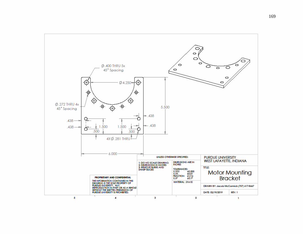
169

170

171