Design and Analysis ofAlgorithms (XI)

LP based Approximation

Guoqiang Li

School of Software, Shanghai Jiao Tong University

Rounding

Set Cover of LP-Rounding

We will design two approximation algorithms for set cover problemusing the method of LP-rounding.

The first one is a simple rounding algorithm achieving a guarantee off .

The second one is based on randomized rounding and achieves aguarantee of O(log n).

The Set Cover LP-Relaxation

min∑S∈S

c(S)xS∑S:e∈S

xS ≥ 1, e ∈ U

xS ≥ 0, S ∈ S

A Simple Rounding Algorithm

Algorithm

1 Find an optimal solution to the LP-relaxation.

2 Pick all sets S for which xS ≥ 1/f in this solution.

Analysis

TheoremThis algorithm achieves an approximation factor of f for the set coverproblem.

Proof.Let C be the collection of picked sets. We first show that C is indeed aset cover.• Consider an element e. Since e is in at most f sets, one of these

sets must be picked to the extent of at least 1/f in the fractionalcover, due to the pigeonhole principle.• Thus, e is covered by C, and hence C is a valid set cover.

Analysis

• The rounding process increases xS, for each set S ∈ C, by a factorof at most f .• Therefore, the cost of C is at most f times the cost of the

fractional cover, thereby proving the desired approximationguarantee.

Randomized Rounding

Why Randomization

The performance guarantee of a random approximation algorithmholds with high probability.

In most cases a randomized approximation algorithms can bederandomized, and

the randomization gains simplicity in the algorithm design andanalysis.

Randomized Rounding for Set Cover

Intuitively, a set with larger value is more likely to be chosen in theoptimal solution.

This motivates us to view the fractions as probability and roundaccordingly.

Analysis (I)

• Let x = p be an optimal solution to the linear program.• For each set S ∈ S, our algorithm pick S with probability pS.• The expected cost of C is

E[cost(C)] =∑S∈S

Pr[S is picked] · cS =∑S∈S

pS · cS = OPTf .

• Next, let us compute the probability that an element a ∈ U iscovered by C.

Analysis (II)

• Suppose that a occurs in k sets of S .• Let the probabilities associated with these sets be p1, . . . , pk .

Then p1 + p2 + · · ·+ pk ≥ 1.• Then we have

Pr[a is covered by C] ≥ 1− (1− 1k

)k ≥ 1− 1e

• To get a complete set cover, independently pick c log n suchsubcollections, and let C′ be their union, where c is a constantsuch that

(1e

)c log n ≤ 14n

Analysis (III)

• Now we have

Pr[a is not covered by C′] ≤ (1e

)c log n ≤ 14n

• Summing over all elements a ∈ U, we get

Pr[C′ is not a valid set cover ] ≤ n · 14n≤ 1

4.

Analysis (IV)

• Clearly E[C′] ≤ OPTf · c log n.• Applying Markov’s Inequality, we get

Pr[cost(C′) ≥ OPTf · 4c log n] ≤ 14

• Thus

Pr[C′ is a valid set cover and has cost ≤ OPTf · 4c log n] ≥ 12

MAX-SAT

MAX-SAT

Given n boolean variables x1, . . . , xn, a CNF

ϕ(x1, . . . , xn) =

m∧j=1

Cj

and a nonnegative weight wj for each Cj.Find an assignment to the xis that maximizes the weight of thesatisfied clauses.

Flipping a Coin

A very straightforward randomized approximation algorithm is to seteach xi to true independently with probability 1/2.

Setting each xi to true with probability 1/2 independently gives arandomized 1

2 -approximation algorithm for weighted MAX-SAT.

Proof

Proof.Let W be a random variable that is equal to the total weight of thesatisfied clauses. Define an indicator random variable Yj for eachclause Cj such that Yj = 1 if and only if Cj is satisfied. Then

W =

m∑j=1

wjYj

We use OPT to denote value of optimum solution, then

E[W ] =

m∑j=1

wjE[Yj] =

m∑j=1

wj · Pr[clause Cj satisfied]

Proof (cont’d)

Since each variable is set to true independently, we have

Pr[clause Cj satisfied] =

(1−

(12

)lj)≥ 1

2

where lj is the number of literals in clause Cj. Hence,

E[W ] ≥ 12

m∑j=1

wj ≥12

OPT .

A Finer Analysis

Observe that if lj ≥ k for each clause j, then the analysis above showsthat the algorithm is a (1− ( 1

2)k)-approximation algorithm for suchinstances. For instance, the performance guarantee of MAX E3SAT is7/8.

From the analysis, we can see that the performance of the algorithm isbetter on instances consisting of long clauses.

TheoremIf there is an (7

8 + ε)-approximation algorithm for MAX E3SAT forany constant ε > 0, then P = NP.

Derandomization

Derandomization

The previous randomized algorithm can be derandomized. Note that

E[W ] = E[W | x1 ← true] · Pr[x1 ← true]

+ E[W | x1 ← false] · Pr[x1 ← false]

=12

(E[W | x1 ← true] + E[W | x1 ← false])

We set b1 true if E[W | x1 ← true] ≥ E[W | x1 ← false] and setb1 false otherwise. Let the value of x1 be b1.

Continue this process until all bi are found, i.e., all n variables havebeen set.

An Example

x3 ∨ x5 ∨ x7

• Pr[clause satisfied | x1 ← true, x2 ← false, x3 ← true] = 1• Pr[clause satisfied | x1 ← true, x2 ← false, x3 ← false] = 1−( 1

2 )2 = 3

4

Derandomization

This is a deterministic 12 -approximation algorithm because of the

following two facts:

1 E[W | x1 ← b1, . . . , xi ← bi] can be computed in polynomialtime for fixed b1, . . . , bi.

2 E[W | x1 ← b1, . . . , xi ← bi, xi+1 ← bi+1] ≥ E[W | x1 ←b1, . . . , xi ← bi] for all i, and by induction,E[W | x1 ← b1, . . . , xi ← bi, xi+1 ← bi+1] ≥ E[W ].

Flipping Biased Coins

Flipping Biased Coins

• Previously, we set each xi true or false with probability 12

independently. 12 is nothing special here.

• In the following, we set each xi true with probability p ≥ 12 .

• We first consider the case that no clause is of the form Cj = xi.

LemmaIf each xi is set to true with probability p ≥ 1/2 independently, thenthe probability that any given clause is satisfied is at leastmin(p, 1− p2) for instances with no negated unit clauses.

Proof

Proof.• If the clause is a unit clause, then the probability the clause is

satisfied is p.• If the clause has length at least two, then the probability that the

clause is satisfied is 1− pa(1− p)b, where a is the number ofnegated variables and b is the number of unnegated variables.Since p > 1

2 > 1− p, this probability is at least 1− p2.

Flipping Biased Coins

Armed with previous lemma, we then maximize min(p, 1− p2),which is achieved when p = 1− p2, namely p = 1

2(√

5− 1) ≈ 0.618.

We need more effort to deal with negated unit clauses, i.e., Cj = xi forsome j.

We distinguish between two cases:

1. Assume Cj = xi and there is no clause such that C = xi. In thiscase, we can introduce a new variable y and replace theappearance of xi in ϕ by y and the appearance of xi by y.

Flipping Biased Coins2. Cj = xi and some clause Ck = xi. W.L.O.G we assume

w(Cj) ≤ w(Ck). Note that for any assignment, Cj and Ck cannotbe satisfied simultaneously. Let vi be the weight of the unit clausexi if it exists in the instance, and let vi be zero otherwise, we have

OPT ≤m∑

j=1

wj −n∑

i=1

vi

We set each xi true with probability p = 12(√

5− 1), then

E[W ] =

m∑j=1

wjE[Yj]

≥ p ·

m∑j=1

wj −n∑

i=1

vi

≥ p · OPT

Rounding by Linear Programming

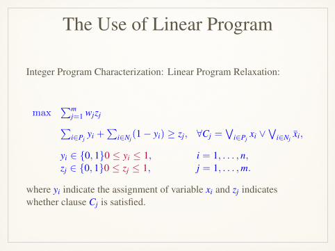
The Use of Linear Program

Integer Program Characterization: Linear Program Relaxation:

max∑m

j=1 wjzj∑i∈Pj

yi +∑

i∈Nj(1− yi) ≥ zj, ∀Cj =

∨i∈Pj

xi ∨∨

i∈Njxi,

yi ∈ {0, 1}0 ≤ yi ≤ 1, i = 1, . . . , n,zj ∈ {0, 1}0 ≤ zj ≤ 1, j = 1, . . . ,m.

where yi indicate the assignment of variable xi and zj indicateswhether clause Cj is satisfied.

Flipping Different Coins

• Let (y∗, z∗) be an optimal solution of the linear program.• We set xi to true with probability y∗i .• This can be viewed as flipping different coins for every variable.

Randomized rounding gives a randomized (1− 1e )-approximation

algorithm for MAX-SAT.

Analysis

Pr[clause Cj not satisfied]

=∏i∈Pj

(1− y∗i )∏i∈Nj

y∗i

≤[

1lj

(∑i∈Pj

(1− y∗i ) +∑

i∈Njy∗i)]lj Arithmetic-Geometric

Mean Inequality

=

1− 1lj

∑i∈Pj

y∗i +∑i∈Nj

(1− y∗i )

lj

≤

(1−

z∗jlj

lj)

Analysis

Pr[clause Cj satisfied]

≥ 1−(

1−z∗jlj

)lj

≥[

1−(

1− 1lj

)lj]

z∗j Jensen’s Inequality

Therefore, we haveE[W ] =

m∑j=1

wj Pr[clause Cj satisfied]

≥m∑

j=1

wjz∗j

[1−

(1− 1

lj

)lj]

≥(

1− 1e

)· OPT

The Combined Algorithm

Choosing the Better of Two

• The randomized rounding algorithm performs better when lj-sare small. (

(1− 1

k

)k is nondecreasing)• The unbiased randomized algorithm performs better when lj-s

are large.• We will combine them together.

Choosing the better of the two solutions given by the two algorithmsyields a randomized 3

4 -approximation algorithm for MAX SAT.

Analysis

Let W1 and W2 be the r.v. of value of solution of randomized roundingalgorithm and unbiased randomized algorithm respectively. Then

E[max(W1,W2)] ≥ E[12

W1 +12

W2]

≥ 12

m∑j=1

wjz∗j

[1−

(1− 1

lj

)lj]

+12

m∑j=1

wj(1− 2−lj

)≥

m∑j=1

wjz∗j

[12

(1−

(1− 1

lj

)lj)

+12(1− 2−lj

)]

≥ 34· OPT

Primal-Dual Schema

Vertex Cover, Revisited Again

Cardinality Vertex Cover

AlgorithmFind a maximal matching in G and output the set of matchedvertices.

(b) (c)

The algorithm

Consider the following algorithm:

1. M ← ∅2. S ← ∅3. while G is not empty do

3.1 Choose an edge e = {u, v} ∈ E(G) and let M ← M ∪ {e}3.2 S ← S ∪ {u, v}3.2 G← G[V \ {u, v}]

4. return S

Cardinality Vertex Cover, Revisit

min∑v∈V

xv

xu + xv ≥ 1, (u, v) ∈ E

xv ≥ 0, v ∈ V

max∑e∈E

ye∑e=(u,v)∈E

ye ≤ 1, u ∈ V

ye ≥ 0, e ∈ E

Vertex Cover

• Vertex Cover Problem is the special case of set cover problemwhen f = 2.• The dual of vertex cover problem is Maximum Matching

Problem.• The duality theorem implies

maximum matching ≤ minimum vertex cover

The algorithm

Consider the following algorithm:

1. M ← ∅2. S ← ∅3. while G is not empty do

3.1 Choose an edge e = {u, v} ∈ E(G) and let M ← M ∪ {e}3.2 S ← S ∪ {u, v}3.2 G← G[V \ {u, v}]

4. return S

This is the combinatorial interpretation of a primal-dual algorithm.

Overview of the Schema

Primal and Dual

min

n∑j=1

cjxj

n∑j=1

aijxj ≥ bi, i = 1, 2, . . . ,m

xj ≥ 0, j = 1, 2, . . . , n

max

m∑i=1

biyi

m∑i=1

aijyi ≤ ci, j = 1, 2, . . . , n

yi ≥ 0, j = 1, 2, . . . ,m

Complementary Slackness

Let x and y be primal and dual feasible solutions, respectively. Then, xand y are both optimal iff all of the following conditions are satisfied:• Primal complementary slackness conditions:

For each 1 ≤ j ≤ n: either xj = 0 or∑m

i=1 aijyi = cj; and• Dual complementary slackness conditions:

For each 1 ≤ i ≤ m: either yi = 0 or∑n

j=1 aijxj = bi.

DiscussionThe theorem ensures

xj > 0 =⇒m∑

i=1

aijyi = cj

In general, we cannot hope

yi > 0 =⇒n∑

j=1

aijxj = bi

We want to show it is not too slack, i.e.

yi > 0 =⇒n∑

j=1

aijxj ≤ β · bi

Complementary SlacknessRelaxation

Let x and y be primal and dual feasible solutions, respectively. Then, xand y are both optimal iff all of the following conditions are satisfied:• Primal complementary slackness conditions:

let α ≥ 1For each 1 ≤ j ≤ n: either xj = 0 or cj/α ≤

∑mi=1 aijyi ≤ cj; and

• Dual complementary slackness conditions:Let β ≥ 1For each 1 ≤ i ≤ m: either yi = 0 or bi ≤

∑nj=1 aijxj ≤ β · bi.

Primal-Dual Schema

Theorem If x and y are primal and dual feasible solutions satisfyingthe conditions stated in the previous page, then

n∑j=1

cjxj ≤ α · βm∑

i=1

biyi

Proof.

n∑j=1

cjxj ≤ αn∑

j=1

(

m∑i=1

aijyi)xj = α

m∑i=1

(

n∑j=1

aijxj)yi ≤ αβm∑

i=1

biyi

• If primal conditions are ensured, we set α = 1• If dual conditions are ensured, we set β = 1.

Primal-Dual ApproximationAlgorithms

1. Formulate a given problem as an IP. Relax the variableconstraints to obtain the primal LP P , then find the dual D.

2. Starts with a primal infeasible solution x and a dual feasiblesolution y, usually x = 0 and y = 0.

3. Until x is feasible, do3.1. Increase the value yi in some fashion until some dual constraints

go tight.3.2. Select some subset of tight dual constraints and increase the

values of primal variables corresponding to these constraints by anintegral amounts. This ensures that the final solution x is integral.

4. The cost of the dual solution is used as a lower bound on OPT .Note that the approximation guarantee of the algorithm is αβ.

Applied to Set Cover

Primal-Dual to Set Cover

min∑S∈S

c(S)xS∑S:e∈S

xS ≥ 1, e ∈ U

xS ≥ 0, S ∈ S

max∑e∈U

ye∑e:e∈S

ye ≤ c(S), S ∈ S

ye ≥ 0, e ∈ U

α = 1 and β = f.

Primal Condition

Primal conditions

∀S ∈ S : xS 6= 0⇒∑e:e∈S

ye = c(S)

• Set S will be said to be tight if∑

e:e∈S ye = c(S).• Since we will increment the primal variables integrally, we can

state the conditions as:• Pick only tight sets in the cover.

Dual Condition

Dual conditions

∀e ∈ U : ye 6= 0⇒∑

S:e∈S

xS ≤ f

• Since we will find a 0/1 solution for x, these conditions areequivalent to:• Each element having a nonzero dual value can be covered at

most f times.

The Algorithm

1. Initialization: x ← 0, y← 02. Until all elements are covered, do:

2.1 Pick an uncovered element, say e, and raise ye until some set goestight.

2.2 Pick all tight sets in the cover and update x.2.3 Declare all the elements occurring in these sets as “covered”.

3. Output the set cover x.

The Guarantee Factor

TheoremThe algorithm achieves an approximation factor of f .

Proof.Clearly there will be no uncovered elements and no overpacked sets atthe end of the algorithm. Thus, the primal and dual solutions will bothbe feasible. Since they satisfy the relaxed complementary slacknessconditions with α = 1 and β = f .

Referred Materials

Content of this lecture comes from Chapter 14 and 15 Chapter 16 in[Vaz04], and Section 5.1-5.5 7.1-7.2 in [WS11].