C H A P T E R 5

P P 1 1 0 - 1 3 0

Descriptive Statistics

Graphing data

Frequency distributions

Bar graphs Qualitative variable (categories)

Bars don’t touch

Histograms

Frequency polygons Quantitative variable (ordinal, interval, or ratio scale)

Others: Pie chart

Stem and leaf

Scatterplot

Example grade distribution

A 1

A- 2

B+ 3

B 7

B- 8

C+ 6

C 3

C- 2

D 1

F 1

N = 34

Class interval

frequency distribution

Graphs!

Read X and Y axis carefully

Death Rates in America

40

60

80

100

120

1980

1981

1982

1983

1984

1985

1986

1987

1988

1989

Year

Nu

mb

er p

er 1

00,0

00 p

op

ula

tion

Age 1-4

Age 15-24

Example bar graph Rauscher, Shaw, & Ky (1993). Mozart Effect

119

111 110

N = 36 college students

Lots of cool graphs!

Florence Nightingale’s “coxcomb” diagram Blue: died of sickness; Red: died of wounds; Black: died of other causes

Graph interpretation

Recency

effect Reminiscence

bump

Careful to read values on each axis – graphs can be deceiving!

Descriptive statistics

Data collected in a study = raw data

Reports of a study = summary data Descriptive statistics provide that summary

Measures of central tendency Describe “middleness” of distribution of scores

Mean

Median

Mode

Measures of variation Describe width or dispersion of a distribution

Range

Standard deviation

Variance

Descriptive statistics

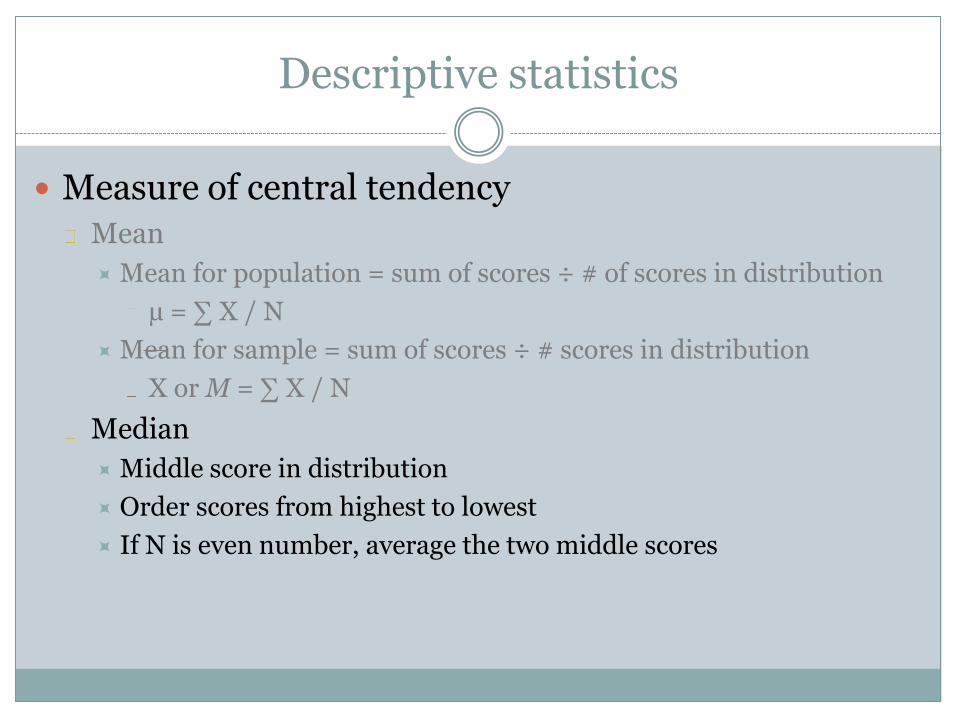
Measure of central tendency

Mean

Mean for population = sum of scores ÷ # of scores in distribution

𝜇 =Σ𝑋 𝑁

Mean for sample = sum of scores ÷ # scores in distribution

M or X =Σ𝑋 𝑁

Mean as the balance point

The mean balances the distances (or deviations) of all scores

Mean

5

5

5

5

Scores (x)

2

2

6

10

Distance from mean

-3

-3

1

5

______ ∑X = 20 N = 4 M = 5

_____ ∑X = 0

Effect of changing 1 score

The mean is not a “robust” statistic It is highly influenced by a single outlier score

26

29

31

32

34

35

38

40

42

83

390

390 / 10

39

____ ∑X = ∑X / N = M =

26

29

31

32

34

35

38

40

42

33

340

340 / 10

34

____ ∑X = ∑X / N = M =

Adding a constant

If you add, subtract, multiply or divide all scores by constant:

The same change is made to M

26

29

31

32

34

35

38

40

42

83

390

390 / 10

39

36

39

41

42

44

45

48

50

52

93

490

490 / 10

49

X + 10

Descriptive statistics

Measure of central tendency

Mean

Mean for population = sum of scores ÷ # of scores in distribution

µ = ∑ X / N

Mean for sample = sum of scores ÷ # scores in distribution

X or M = ∑ X / N

Median

Middle score in distribution

Order scores from highest to lowest

If N is even number, average the two middle scores

Calculating the median for RTs

512 587 590 578 567 533 573 529 577 572 572 591 575 577 534

512 529 533 534 567 572 572 573 575 577 577 578 587 590 591

512 587 590 578 567 533 573 529 899 572 572 591 575 577 534

512 587 590 578 567 533 573 529 177 572 572 591 575 577 534

sorted scores

573 564.47

Median

Mean

573 585.93

572 537.80

Add Hi X Add Lo X

Median is

a robust

statistic!

Descriptive statistics

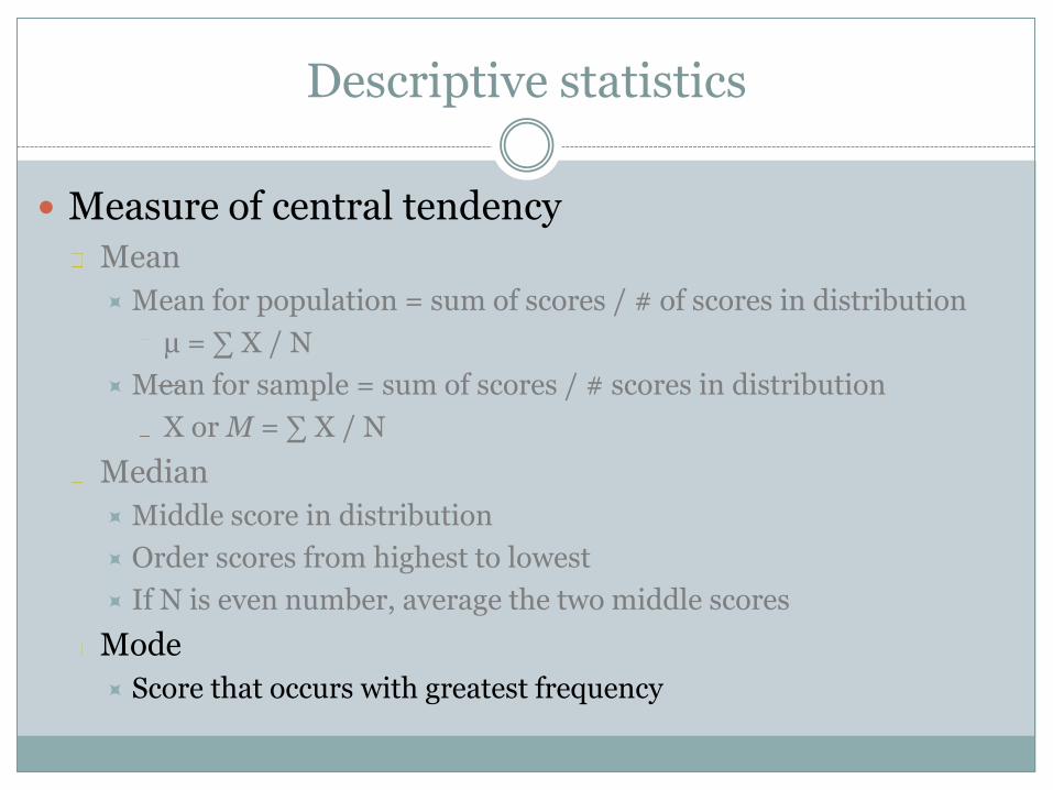
Measure of central tendency

Mean

Mean for population = sum of scores / # of scores in distribution

µ = ∑ X / N

Mean for sample = sum of scores / # scores in distribution

X or M = ∑ X / N

Median

Middle score in distribution

Order scores from highest to lowest

If N is even number, average the two middle scores

Mode

Score that occurs with greatest frequency

Example grade distribution

A 1

A- 2

B+ 3

B 7

B- 8

C+ 6

C 3

C- 2

D 1

F 1

N = 34

M = 80.38

Median = 81

Mode = B-

Can have 2+ modes

Sample grade distribution with 2 modes

0

1

2

3

4

5

6

7

A A- B+ B B- C+ C C- D F

Types of distributions

Normal distribution

Bell-shaped

Symmetrical

Only 1 mode

Mean, median, mode all equal

Kurtosis: spread of distribution

How flat or peaked

Mesokurtic: medium peak (like normal distribution)

Leptokurtic: tall and thin

Platykurtic: flat and broad

Measures of central tendency Indicators of the shape of the distribution

How mean, median, and mode change w/ shape of distribution

Normal distribution

Positive skew

Tail to positive scores

Negative skew

Tail to negative scores Positive skew Negative skew

Which measure of central tendency to use?

If interval or ratio data and normally-distributed

Use mean

If interval or ratio data and there are outliers or a skewed-distribution

Use median

If nominal data

Use mode But, that’s not enough info …

Measures of variation

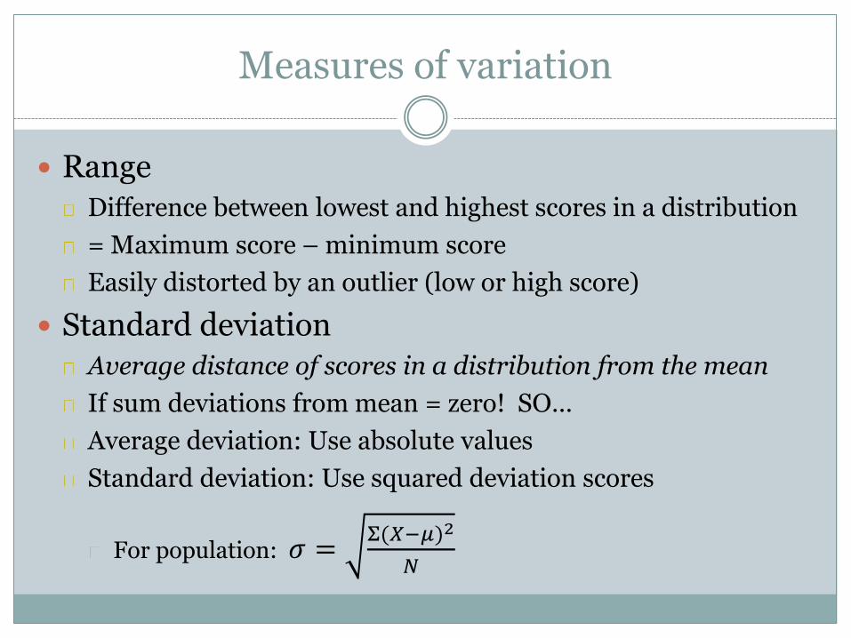
Range

Difference between lowest and highest scores in a distribution

= Maximum score – minimum score

Easily distorted by an outlier (low or high score)

Standard deviation

Average distance of scores in a distribution from the mean

If sum deviations from mean = zero! SO…

Average deviation: Use absolute values

Standard deviation: Use squared deviation scores

For population: 𝜎 =Σ(𝑋−𝜇)2

𝑁

Example grade distribution

A 1

A- 2

B+ 3

B 7

B- 8

C+ 6

C 3

C- 2

D 1

F 1

N = 34

M = 80.38

Median = 81

Mode = B-

s = 7.92

M = 80.38 M + s = 88.3 M - s = 72.5

Note: most scores are w/in 8 pts of mean

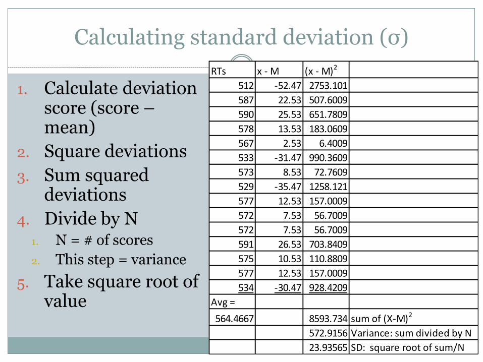
Calculating standard deviation (σ)

RTs x - M (x - M)2

512 -52.47 2753.101

587 22.53 507.6009

590 25.53 651.7809

578 13.53 183.0609

567 2.53 6.4009

533 -31.47 990.3609

573 8.53 72.7609

529 -35.47 1258.121

577 12.53 157.0009

572 7.53 56.7009

572 7.53 56.7009

591 26.53 703.8409

575 10.53 110.8809

577 12.53 157.0009

534 -30.47 928.4209

Avg =

564.4667 8593.734 sum of (X-M)2

572.9156 Variance: sum divided by N

23.93565 SD: square root of sum/N

1. Calculate deviation score (score – mean)

2. Square deviations

3. Sum squared deviations

4. Divide by N 1. N = # of scores

2. This step = variance

5. Take square root of value

Calculating standard deviation (s)

1. Calculate deviation score (score – mean)

2. Square deviations

3. Sum squared deviations

4. Divide by N or N - 1 1. This step = variance

2. Use N for population

3. Use N-1 to estimate population from sample

5. Take square root of value

RTs x - M (x - M)2

512 -52.47 2753.101

587 22.53 507.6009

590 25.53 651.7809

578 13.53 183.0609

567 2.53 6.4009

533 -31.47 990.3609

573 8.53 72.7609

529 -35.47 1258.121

577 12.53 157.0009

572 7.53 56.7009

572 7.53 56.7009

591 26.53 703.8409

575 10.53 110.8809

577 12.53 157.0009

534 -30.47 928.4209

Avg =

564.4667 8593.734 sum of (X-M)2

sd = 613.8381 Variance: sum divided by N-1

24.77576 = 24.77576 SD: square root of sum/N-1

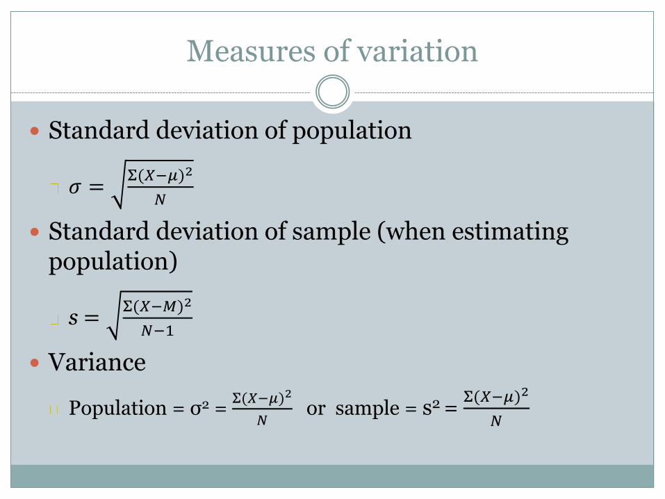
Measures of variation

Standard deviation of population

𝜎 =Σ(𝑋−𝜇)2

𝑁

Standard deviation of sample (when estimating population)

s =Σ(𝑋−𝑀)2

𝑁−1

Variance

Population = σ2 = Σ(𝑋−𝜇)2

𝑁 or sample = s2 =

Σ(𝑋−𝜇)2

𝑁

Why use N – 1 ?

Sample is less variable than the population Divide by smaller # so yields more conservative estimate

of variance or SD Makes variance score larger

Use n-1 so can make conclusions about population (not just describe your sample)

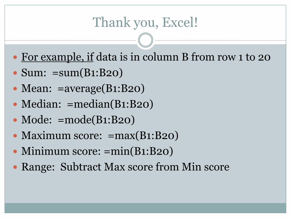
Thank you, Excel!

For example, if data is in column B from row 1 to 20

Sum: =sum(B1:B20)

Mean: =average(B1:B20)

Median: =median(B1:B20)

Mode: =mode(B1:B20)

Maximum score: =max(B1:B20)

Minimum score: =min(B1:B20)

Range: Subtract Max score from Min score