descriptive econometrics for non-stationary time series - the cowles

DESCRIPTIVE ECONOMETRICS FOR NON-STATIONARY TIME SERIES WITH EMPIRICAL ILLUSTRATIONS

BY

PETER C. B. PHILLIPS

COWLES FOUNDATION PAPER NO. 1023

COWLES FOUNDATION FOR RESEARCH IN ECONOMICS YALE UNIVERSITY

Box 208281 New Haven, Connecticut 06520-8281

2001

http://cowles.econ.yale.edu/

JOURNAL OF APPLIED ECONOMETRICSJ. Appl. Econ. 16: 389–413 (2001)DOI: 10.1002/jae.600

DESCRIPTIVE ECONOMETRICS FOR NON-STATIONARY TIMESERIES WITH EMPIRICAL ILLUSTRATIONS

PETER C. B. PHILLIPS*Cowles Foundation for Research in Economics, Yale University, PO Box 208281, New Haven, CT 06520-8281, USA

SUMMARYRecent work by the author on methods of spatial density analysis for time series data with stochastic trendsis reviewed. The methods are extended to include processes with deterministic trends, formulae for the meanspatial density are given, and the limits of sample moments of non-stationary data are shown to take theform of moments with respect to the underlying spatial density, analogous to population moments of astationary process. The methods are illustrated in some empirical applications and simulations. The empiricalapplications include macroeconomic data on inflation, financial data on exchange rates and political opinionpoll data. It is shown how the methods can be used to measure empirical hazard rates for inflation anddeflation. Empirical estimates based on historical US data over the last 60 years indicate that the predominantinflation risks are at low levels (2–6%) and low two-digit levels (10–12%), and that there is also a significantrisk of deflation around the �1% level. Copyright 2001 John Wiley & Sons, Ltd.

1. INTRODUCTION

A guiding principle in much of Denis Sargan’s research was the ‘marriage’ of time series andsimultaneity. In one of his earliest published papers, Sargan (1953) studied the properties ofthe correlogram and periodogram. Subsequently, his work (1958, 1959) on instrumental variablesprovided a methodology of estimation that was well suited to the joint treatment of simultaneity andtime series dynamics in parametric models. Later on, his work with Espasa (1977) sought solutionsto much more general time series regression problems in the presence of simultaneity. Inspired bythe work of Hannan (1963), these solutions utilized spectral methods which permit an investigatorto be agnostic with respect to the time series properties of the errors in an econometric model.These methods now fall into the category of semiparametric approaches to modelling, treating theerrors, as they do, in a non-parametric fashion while leaving the systematic components of themodel in parametric form. Since this early work, non-parametric and semiparametric approachesto econometric modelling have grown in popularity in both time series and microeconometricapplications. In view of the common lack of prior information from economic theory modelsabout dynamic formulations, the use of these methods in time series contexts has seemed highlydesirable to many researchers including those who have argued for the use of unrestricted vectorautoregressions (Sims, 1980). Spectral methods, like unrestricted VARs, can be regarded as toolsfor describing the data and it is this rather more general subject that concerns us in the presentpaper.

Ł Correspondence to: Professor P. C. B. Phillips, Cowles Foundation for Research in Economics, Yale University, P.O.Box 208281, New Haven, CT 06520-8281, USA. E-mail: [email protected]/grant sponsor: NSF; Contract/grant number: SES 94-22922; SBR-9730295.

Copyright 2001 John Wiley & Sons, Ltd. Received 19 January 1999Revised 9 August 2000

390 P. C. B. PHILLIPS

Description is the starting point in much empirical work. In almost all econometric applicationsit is common to look at the data that has been collected, and find ways of revealing what seem tobe its principal features. Graphical representations taking the form of time series plots and chartsgive us particularly useful ways of envisioning information and conducting comparative analysesover time. Tellingly these methods appear both in formal applied econometric analysis and in thepopular press, where they figure prominently in business page discussions of the behaviour ofeconomic time series like asset prices, exchange rates, business confidence and production. Ofcourse, while it is relatively easy to point informally to characteristics that such data seem todisplay in visual plots and charts (and this is, indeed, what is done daily in the popular businesspress), it is rather a different matter to formalize this process of description.

In describing the characteristics of economic time series, we are greatly assisted by a presumptionof stationarity. For then we can utilize time invariant parameters like the mean, the variance, and theautocorrelogram to build a groundwork of descriptive statistics which involve the sample analoguesof these quantities. These parameters provide points of bearing that are useful in summarizing aparticular series and in comparing different series. Extending the groundwork further, there arethe underlying time invariant marginal and finite dimensional probability densities of the data aswell as its spectral density and higher-order spectra, all functional quantities that can be estimatedfrom the observed data in terms of sample analogue functions. While inferential procedures canand, indeed, have been developed for all these quantities, they are first and foremost descriptivetools.

Unfortunately, this entire groundwork of descriptive statistics gets lost when the presumptionof stationarity is removed because the underlying time invariant quantities no longer exist. Thesample analogues are still, of course, computable in the same way, but their interpretation is not thesame and they typically no longer converge without restandardization as the sample size increases.Instead, in many cases of interest like time series that have random wandering characteristics, thesesample analogues end up having random rather than non-random limits, as shown in Phillips (1986,1987, 1988). Notwithstanding this random limiting behaviour, it remains of interest whether anyof these sample analogues continue to be useful as descriptive tools for non-stationary data and,if they are, how they should be interpreted.

It is little exaggeration to say that there are presently in use no tools of descriptive statisticsfor non-stationary data. In recent work, the Phillips (1998a) suggested some methods of spatialdensity analysis that apply in a fairly natural way to non-stationary data with stochastic trends andmade a start in addressing the questions just raised in the last paragraph. This paper reviews thosemethods, shows how they may be extended to more general processes and gives some illustrationsof the methods in practical empirical work and simulations. The empirical applications chosenfor this paper include macroeconomic data on inflation, financial data on exchange rates andpolitical opinion poll data. In the inflation application, it is shown how the methods can be usedto measure historical hazards for inflation and deflation, the former being of interest in view ofrecent inflation-targeting policies by monetary authorities in several countries, and the latter beingof interest in view of recent experience in the Asian economies.

The paper is organized as follows. Section 2 outlines the spatial density techniques given inPhillips (1998a) and the backbone of limit theory that justifies these descriptive methods. Guidanceon the practical interpretation of these results in applications is provided and some extensions ofthese methods to processes with deterministic trends and long-memory components are discussed.Formulae for the mean spatial density are derived, and the theory is used to show how samplemoments of non-stationary data have limits that can be expressed as moments with respect to an

Copyright 2001 John Wiley & Sons, Ltd. J. Appl. Econ. 16: 389–413 (2001)

DESCRIPTIVE NON-STATIONARY ECONOMETRICS 391

underlying spatial density. These moments therefore continue to provide descriptive characteristicsof the data in the limit, in spite of non-stationarity, and thereby retain their use as summarystatistics. Section 3 gives some illustrations of the methods with simulated data. Section 4 reportsempirical applications to inflation, exchange rates and opinion poll data. Section 5 makes someconcluding comments in relation to more general issues of econometric methodology. Notation issummarized in Section 6.

2. CONCEPTS, BACKGROUND THEORY, AND ASYMPTOTICS

2.1. Preliminaries

To fix ideas and facilitate the development, we suppose that the data are well modelled bya stochastic trend with a single unit root. The theory discussed here was initiated in Phillips(1998a) and Phillips and Park (1998) and subsections 2.2–2.4 and 2.6–2.7 overview the particularmethods from those papers that we will use here. These ideas are shown in sub-section 2.8 to berelevant in interpreting the sample moments of non-stationary data. The distribution of the spatialdensity is discussed and its mean functional is calculated in sub-section 2.9. Extensions of theideas to processes with deterministic trends are given in sub-section 2.10. Further extensions tomore general cases, like time series with fractional roots or near unit roots, are presently underdevelopment and are briefly mentioned also. These are likely to be important in empirical workwhere there is evidence of long-range dependence or fractional stochastic trends. The methods weare about to discuss continue to be applicable in such cases in their present form, but with somechanges in the technical details and limit theory that are in the process of being worked out.

Accordingly, this paper mainly concentrates on a unit root time series yt D t1us, whose

increments ut form a stationary time series with zero mean and finite absolute moments to orderp > 2, and which satisfies the functional law:

YnÐ� D y[nÐ]pn

) BÐ� � BM�2� 1�

Here, �2 is the long-run variance of ut, or 2�fuu0�, where fuu is the spectrum of ut. Primitiveconditions for equation (1) are well known (e.g. see Phillips and Solo, 1992) and we do not pursuethem here. In fact, we need to go a little further than equation (1) and arrange the probability spacein such a way that the processes Yn and B lie in the same space. This can be accomplished byembedding arguments. In particular, we can use the Hungarian strong approximation (e.g. Csorgoand Horvath, 1993) to yt, which enables the construction of an expanded probability space thatincludes a Brownian motion BÐ� for which:

sup0�k�n

jyk � Bk�j D oa.s.n1/p�

so that

sup0�k�n

∣∣∣∣ ykpn

� B

(k

n

)∣∣∣∣ D oa.s.1� 2�

Since Ynr� D yt�1/pn�, for t � 1�/n � r < t/n, t > 1, we get the direct representation:

Ynr� D B

([nr]

n

)C oa.s.1� 3�



which effectively embeds the process Yn in the Brownian motion B. Nothing will be lost if weproceed as if the space has already been set up to ensure equation (3).

When dealing with more general time series than a unit root, we need to establish (or appeal to)appropriate embeddings that extend equation (3) and adjust the probability space correspondingly.Thus, if yt D ˇt C t

1us D ˇt C y0t is a unit root process with drift, we can arrange the space so

that:

Y0nr� D y0

[nr]pn

D B0(

[nr]

n

)C oa.s.1�

and then:Ynr� D y[nr] D ˇnr C B0[nr]� C oa.s.

pn�

in place of equation (3). Similarly, if yt D t1e

t�j�c/nuj is a near unit root process with local tounity coefficient c, then yt can be embedded in a diffusion process Jcr� D ∫ r

0 er�s�cdBs� and thefollowing strong approximation (see lemma A3 of Phillips, 1998b) holds:

supr2[0,1]

∣∣∣∣y[nr]pn

� Jcr�

∣∣∣∣ D oa.s.1�

giving:

Ynr� D y[nr]pn

D Jc

([nr]

n

)C oa.s.1�

in place of equation (3).

2.2. Sojourn Time and Spatial Density

A central idea in the spatial density analysis of Phillips (1998a) is to replace the notion of atime invariant marginal probability density with that of a time dependent stochastic process thatmeasures spatial density as it has occurred over a given temporal trajectory of the time series.However, instead of measuring probability density at spatial points, this alternate quantity measuresthe density contributed at different spatial points towards the total quadratic variation of the processover a given interval of time. We explain this difference as follows.

If Xt is a strictly stationary time series with absolutely continuous distribution and probabilitymeasure P, then its time invariant probability density can be written in terms of the formula:

pdf Xs� D limε!0

1

2ε

∫1jx � sj < ε�dP 4�

Accordingly, as this definition makes clear, the quantity pdf Xs� measures the contribution to theoverall probability P that comes from around the spatial point s. Inverting equation (4), we getfor a measurable set A:

PXt 2 A� D∫

1A�dP D∫A

pdf Xs�ds 5�

For a non-stationary series like yt, there is no time invariant probability measure P and it is nolonger sensible to think of decomposing probability into densities from different spatial regions.Moreover, each trajectory yt: t D 1, . . . , n� has its own special characteristics, as does that ofthe limit Brownian motion process B. In view of equations (1) and (3), it is simplest to replace



the time index t with the index r representing the fraction of the sample included in the seriesby time t. Then, the corresponding trajectories of the series and the limit process are given byYnr�: r 2 [0, 1]� and Br�: r 2 [0, 1]�. The quadratic variation of the limit process B is givenby the square bracket process:

[B]r D∫ r

0dB�2 D r�2 6�

which is a simple linear deterministic function of r in this Brownian motion case. Over the fullsample (i.e. when r D 1), the total quadratic variation of the limit process B is simply �2. Wemay therefore contemplate decomposing this variation into densities from different spatial regionsaccording to:

LBr, s� D limε!0

1

2ε

∫ r

01jBt� � sj < ε�d[B]t 7�

The limit in equation (7) is known to exist almost surely and the limit function LBr, s� is calledthe local time of the Brownian motion B at the spatial point s. LBr, s� is a continuous stochasticprocess in both its temporal and spatial arguments and it measures the sojourn time that the processB spends in the vicinity of s over the time interval [0, r]. Obviously, it is increasing in r (i.e.as more time elapses, the number of visits to s, and hence the density there, can only increase).These properties of the local time process of Brownian motion are rather well known (e.g. Revuzand Yor, 1994).

Just as we can invert equation (4) to form (5), we may invert (7) to deliver the occupation time(in variational units) that B spends in the set A over the time interval [0, r], i.e.:∫ r

01Bt� 2 A� d[B]t D

∫ALBr, s� ds

When A is the whole real line, this formula produces the decomposition:

[B]r D∫ 1

�1LBr, s� ds

which, in view of equation (6), leads quite simply to:

�2 D∫ 1

�1LB1, s� ds 8�

an expression that breaks down the variance of B(1) (i.e. the limiting variance of Yn1�) into thecontributions associated with each spatial point s visited by B (respectively, Yn). Standardizingequation (8) by ��2 we have:

1 D∫ 1

�1LB1, s� ds

where:

LB1, s� D ��2LB1, s� D limε!0

1

2ε

∫ 1

01jBt� � sj < ε� dt 9�

is chronological local time in the sense that it measures sojourn time at s purely in chronologicalunits (rather than variance based units). LB1, s� is normalized so that the total amount oftime spent by the process in the vicinity of all points that it could possibly visit is unity



(i.e. the length of the time interval [0, 1] over which the process has been active). Similarly,LBr, s� D ��2LBr, s� D limε!01/2ε�

∫ r0 1jBt� � sj < ε� dt and r D ∫1

�1 LBr, s� ds.Roughly speaking, we can think of LB1, s� as the proportion of time over the unit interval

[0, 1] that B spends in the vicinity of the spatial point s. Similarly, LBr, s� can be interpretedas the proportion of time over the interval [0, r] that B spends in the vicinity of the spatialpoint s.

2.3. Estimating a Spatial Density

We can construct spatial measures for the observed time series yt that are similar to the measureLB1, s� for the sojourn time of Brownian motion. In particular, the quantity:

n∑tD1

1(∣∣∣∣ ytp

n� s

∣∣∣∣ < εn

)simply counts the number of times yt/

pn� lies within εn of s, and so the quantity:

1

2εn

1

n

n∑tD1

1(∣∣∣∣ ytp

n� s

∣∣∣∣ < εn

)D 1

2εn

∫ 1

01jYnr� � sj < εn�dr 10�

measures the relative amount of time that yt/pn� lies within εn of s, given the total number of

observations (n) and the length of the interval 2εn�. In view of the embedding equation (3), (10)is approximately:

1

2εn

∫ 1

01jBr� � sj < εn�dr 11�

whose limit as εn ! 0, according to equation (9), is LB1, s�. Thus, equation (10) is an empiricalestimate of the chronological time, LB1, s�, spent by the limit process B in the vicinity of thespatial point s. We can think of (10) as a spatial density estimate constructed with a uniformkernel and with bandwidth parameter εn. Using a general kernel function KÐ� in place of auniform kernel, we would have the estimate:

LB1, s� D 1

n

1

εn

n∑tD1

K

(1

εn

(s � ytp

n

))where KÐ� is a symmetric, non-negative function that integrates to unity. Setting KεÐ� D1/ε�KÐ/ε�, we can rewrite this formula as:

LB1, s� D 1pn

1pnεn

n∑tD1

K

(1pnεn

pns � yt�

)

D 1pn

1

hn

n∑tD1

K

(1

hnpns � yt�

)

D 1pn

n∑tD1

Khnpns � yt� 12�



or as

LB

(1,

apn

)D 1p

n

n∑tD1

Khna � yt� 13�

both of which are expressed as a kernel function in terms of the original series yt.The bandwidth parameter in equation (12) is hn D p

nεn and the spatial position, a D pns, is

now measured in units ofpn. As is apparent from equation (11), it is important that εn ! 0 if

we are to achieve a consistent estimate of the local time LB (1, s). However, it is no longer vitalthat hn ! 0, and, indeed, LB (1, s) may still be consistent for LB (1, s) even when hn is constantor slowly increasing. The reason is that in conventional kernel density estimation for stationaryprocesses a shrinking bandwidth serves the purpose of focusing attention on a particular spatialpoint, whereas in the present situation yt tends naturally on its own to drift away from any givenspatial point at the rate

pn. So, on the one hand, there is less reason to have to focus attention

on given spatial points, because this focus occurs in a natural way. But, on the other hand, thereare necessarily a reduced number of relevant observations in estimating the spatial density LB

(1, s). In fact, there are only Opn� relevant observations to each spatial point, compared with

the usual O(n) relevant observations in stationary density estimation. In effect, this is becausethe number of returns that a unit root process, like a random walk, makes to the origin or someother fixed point is of the order of

pn (cf. Feller, 1957, p. 83), whereas all n observations of a

stationary times series are relevant in fitting its probability density at any point in the support.This difference in the order of magnitude explains the standardizing factor 1/

pn that appears in

equation (12). By contrast, if Xt is a strictly stationary time series with probability density (4),then the corresponding kernel density estimate is given by:

pdf Xs� D 1

n

n∑tD1

Khns � Xt� D 1

n

1

hn

n∑tD1

K

(1

hns � Xt�

)14�

where the standardizing factor is 1/n and the bandwidth parameter hn ! 0.

2.4. Limit Theory

Under some rather weak regularity conditions that are discussed in Phillips (1998a) it is shownthat:

LBr, s� D 1pn

[nr]∑tD1

Khnpns � yt� !a.s. LBr, s � B0(�� 15�

This result allows for non-trivial initial conditions in the process yt D t1us C y0, showing that the

point s � B0(�� at which the spatial density is estimated may be affected by initial conditions ifthese are not Op1�. In particular, if the initial conditions extend into the distant past as in:

y0 D[n(]∑jD0

u�j, for some ( ½ 0

for which the following functional law holds:

n� 12

[n(]∑jD0

u�j ) B0(�



then in place of equation (1) we have:

n� 12 y[nr] ) Br� C B0(�

with the Brownian motions B and B0 being independent. Again, matters can be arranged so thatthe probability space of yt includes B0.

A limit distribution theory for the estimate OLBr, s� is also available. Indeed, using thenormalization factor cn D 1/εn D p

n/hn, we have the following mixed normal limit theory(Phillips, 1998a):

pcn[ OLBr, s� � LBr, s � B0(��] ) MN0, 16K2LBr, s � B0(�� 16�

where the constant is:

K2 D∫ 1

0

∫ 1

0Kp�p ^ t�Kt�dpdt

a quadratic functional of the kernel K and the covariance function of Brownian motion. When K is anormal kernel, K2 D ��1/221/2 � 1�. The convergence rate in equation (16) is

pcn D n1/4/

phn,

which is slower than the conventional rate of convergence of kernel density estimates in thestationary case (i.e.

pnhn) for all bandwidths hn D c/nb with b < 1/4.

Using equation (16), asymptotic confidence intervals for LBr, s � B0(�� can be constructed ateach spatial point, giving e.g.:

OLBr, s� š 1.96

(16K2 OLBr, s�

cn

) 12

as a 95% confidence interval for LBr, a � B0(��. By virtue of the standardization of yt, thequantities measure spatial departures from the origin in units of

pn and the spatial points are

centred on a standardized initial condition. Hence, for a confidence interval directly at the points0, we would compute:

OLB

(r, s0 C n� 1

2 y0

)š 1.96

16K2 OLB

(r, s0 C n� 1

2 y0

)cn

12

17�

These intervals can be compared with the confidence intervals of kernel estimates of a stationaryprobability density like equation (15). By traditional theory (Silverman, 1986) a 95% confidenceinterval for the probability density pdf Xs� is:

pdf Xs� š 1.96

(k2pdf Xs�

nh

) 12

18�

where:

k2 D∫ 1

�1Kr�2dr 19�



Leaving aside initial conditions, the only differences between equations (17) and (18) are in thescale factors and the convergence rate. The former arises because of persistent temporal dependencein the trajectory of yt, and the latter because of the effective number of observations. In otherrespects, (17) simply extends the theory of non-parametric density estimation to spatial densityestimation for stochastic processes.

2.5. Interpreting Spatial Density Estimates

The interpretation of spatial density estimates like LBr, s� is similar to that of a conventionalprobability density estimate. As indicated earlier, in rough terms LB1, s� is the proportion oftime over the unit interval [0, 1] that the limit process B spends in the vicinity of the spatialpoint s. Similarly, the quantity LBr, s� is an estimate of the proportion of time over [0, r] thatthe standardized series yt/

pn spends in the vicinity of s. The quantity LBr, a/

pn� is then an

estimate of the proportion of time over [0, r] that the series yt spends in the vicinity of a. Notethat: ∫ 1

�1LB

(1,

apn

)da D

∫ 1

�1LB1, s�ds

pn D p

n

so that on this adjusted scale of spatial measurement the total amount of sojourn time is set topn rather than unity. With this modification, we can think of spatial density estimates just like

conventional density estimates, the difference being that in the latter we are distributing probabilityacross space whereas in the former we are distributing sojourn time across space. As is apparentfrom equations (13) and (14), the same formula applies in each case up to normalization by

pn.

Thus if we use the spatial density estimate (13) in the case of stationary rather than non-stationarydata we will obtain the usual kernel density estimate scaled by

pn. In that case, we are effectively

distributing a non-unitarypn probability across spatial points, rather than the

pn sojourn time.

2.6. Hazard Functions

Following Phillips (1998a), we define the spatial hazard function HBr, a� associated with a givenspatial density LBr, s� as follows:

HBr, a� D LBr, a�∫ 1

aLBr, s�ds

20�

This definition is entirely analogous to the hazard rate ,x� associated with a continuous probabilitydensity pdf Xx�, which has the form:

,x� D pdf Xx�∫ 1

xpdf Xs�ds

D pdf Xx�

1 � cdf Xx�D pdf Xx�

Fx�

where cdf Xx� is the cdf of the distribution and Fx� D 1 � cdf Xx� is the survival function. It isalso useful to define the left-sided hazard:

hBr, a� D LBr, a�∫ a

�1LBr, s�ds

21�



The functions (20) and (21), like the spatial density LBr, a� itself, have two arguments; time andspace. Note that HB and hB are invariant to whether LBr, a� or LBr, a� are used in definitions(20) and (21).

The spatial hazard functions can be interpreted as follows. HBr, a� measures the conditionallikelihood computed over the sample path to time r that B takes the value a, given that it takesvalues at least as big as a. Similarly, hBr, a� measures the conditional risk computed over thesame sample path to time r that B takes the value a, given that it takes values at least as small asa. To be more concrete, suppose the time series yt is inflation and that B(r) is the weak limit ofn�1/2y[nr]. The spatial hazard HBr, a D s/

pn� then measures the conditional likelihood computed

over the period [0, r] (which is expressed in standardized units of fractions of the overall sample,so that it corresponds to an observation period of t D p

nr for yt) of an inflation rate of s, giventhat inflation is at least as great as s. Similarly, hBr, a D s/

pn� measures the conditional risk

computed over the period [0,r] (respectively, an observation period of t D pnr for yt) of an

inflation rate of s, given that inflation is at least as small as s. In the latter case, when s is negativewe can think of hBr, a D s/

pn� as measuring the hazard of deflation rather than inflation. That

is, if there is deflation, hBr, a D s/pn� measures the relative likelihood of a deflation rate of s.

For a given time period r, the shape of the spatial hazard rate functions HBr, a D s/pn� and

hBr, a D s/pn� can be studied in just the same way as we look at hazard rates in the analysis of

independent (or strictly stationary) data. In such studies it is usually of interest to find out whetherthe hazard declines, increases or stays constant as we increase s, whether there are multiple peaksin the hazard and so on. Since our hazard rates also depend on time r, we can consider whathappens to the hazard rate functions as the time period changes or as new data is introduced. Inthe case of inflation, this means that we look at whether the hazard of a certain rate of inflationof deflation rises or falls over time.

2.7. Hazard Functions Asymptotics

The spatial hazard functions HBr, a� and hBr, a� are empirically estimable using the non-parametric spatial density estimate LBr, s/

pn�. In particular, we may construct:

HB

(r,

spn

)D LBr, s/

pn�∫ 1

aLBr, p/

pn�dp/

pn�

, hB

(r,

spn

)D LBr, s/

pn�∫ a

�1LBr, p/

pn�dp/

pn

These estimators are consistent and have mixed normal distributions under the same regularityconditions as the limit theory for the spatial density estimate LBr, s/

pn�. In particular, we have:

HB

(r,

spn

)!a.s. HBr, a � B0(��, hB

(r,

spn

)!a.s. hBr, a � B0(��

and:

pcn

[HB

(r, n� 1

2 s

)� HBr, a � B0(��

]) 4MN

(0, K2

HBr, a � B0(��2

LBr, a � B0(��

)pcn

[hB

(r, n� 1

2 s

)� hBr, a � B0(��

]) 4MN

(0, K2

hBr, a � B0(��2

LBr, a � B0(��

)Copyright 2001 John Wiley & Sons, Ltd. J. Appl. Econ. 16: 389–413 (2001)


The results for HBr, n�1/2s� are proved in Phillips (1998a) and those for hBr, n�1/2s� follow ina similar way.

2.8. Interpreting Moments

In stationary cases, the ergodic theorem and the existence of moments are all that are required toensure good limiting behaviour of sample moments. Thus, if Xt is strictly stationary and ergodic,and Xk

t is integrable then:

n�1n∑

tD1

Xkt !a.s. EX

kt 22�

a result that allows us to interpret sample moments of integrable functions of the data in terms ofpopulation moments.

In non-stationary cases, the absence of ergodicity means that quite different limiting behaviourcan be expected of sample moments than what occurs in equation (22). Nevertheless, samplemoments still play a role as descriptive statistics for the sample data, because they continue tosummarize key features of the data in much the same way as in the stationary case. In manycases, empirical investigators want to characterize the data by some data-reduction techniqueswithout having to resolve potentially complicated issues like choosing between stationary andnon-stationary generating mechanisms. Thus, it is of interest to be able to interpret sample momentcharacteristics for non-stationary data.

For a time series yt satisfying equation (1), it is now a very well-known application of functionallimit theory and continuous mappings (Phillips, 1986, 1987, 1988) that standardized moments ofyt have the following asymptotic behaviour:

1

n1C k2

n∑tD1

ykt )

∫ 1

0Br�kdr 23�

There is another way of writing this result. We use the fact that if g is a measurable and locallyintegrable map then: ∫ 1

0gBr�� dr D

∫ 1

�1gs�LB1, s� ds 24�

This result, known as the occupation time formula (Revuz and Yor, 1994), converts temporalintegrals into spatial integrals involving local time. We have written formula (24) here in terms ofchronological local time LB1, s�. Applying formula (24) to (23) reveals that we have the alternaterepresentation:

1

n1C k2

n∑tD1

ykt D 1

n

n∑tD1

(ytpn

)k

)∫ 1

�1skLB1, s� ds 25�

which is the kth moment of the spatial distribution LB1, s�. In effect, sample momentsof yt converge weakly to corresponding sample moments of the spatial distribution of thelimit process. In this form, (25) is a very natural analogue of (22). Moreover, it makes itclear the sense in which sample moments continue to be useful descriptive characteristics of



the data. Whether the data are stationary or non-stationary, sample moments provide sum-mary information about the observed data that reflect characteristics of an underlying popu-lation. This population is just the stationary distribution in the case of a stationary, ergodictime series, whereas it is the sojourn distribution of the limit process in the non-stationarycase.

2.9. The Distribution of the Spatial Density Process

Since the spatial density is a random process, it helps in understanding its behaviour to know moreabout its probability distribution and some of its characteristics. If Wt� is standard Brownianmotion, then the probability density of the local time LWr, s� changes according to the values ofthe arguments r and s. The density is also influenced by initialization of the process. For W0� D 0and for s D a > 0 the density of LWr, s� is:

fy� D√

2

�re� yCa�2

2r

Perhaps, the most important single characteristic of this distribution is the mean spatial densityELWr, a��. At the spatial value s D a > 0, the mean is calculated as follows:

ELWr, a�� D√

2

�r

∫ 1

0ye� yCa�2

2r dy

D√

2

�r

∫ 1

az � a�e� z2

2r dz

D 1

2

√2

�r

∫ 1

a2

(q

12 � a

)e� q

2r q� 12 dq

D 1

2

√2

�r

[∫ 1

a2e� q

2r dq � a∫ 1

a2e� q

2r q� 12 dq

]D√

2r

�

[∫ 1

a2/2re�pdp � a2r�� 1

2

∫ 1

a2/2re�pp� 1

2 dp

]

D√

2r

�e� a2

2r � ap�

(1

2,a2

2r

)26�

where b, x� D ∫1x e�ppb�1dp is an incomplete gamma function. Combining equation (26) with

a similar calculation for s D a < 0, we end up with the general formula:

ELWr, a�� D√

2r

�e� a2

2r � jajp�

(1

2,a2

2r

)27�

and the mean spatial density function is seen to be symmetric about the origin a D 0. The functionis graphed in Figure 1.

More complex calculations can be performed to produce a related result for the mean local timeof a Brownian motion with drift and these will be reported elsewhere.



0.8

0.7

0.6

0.5

0.4

0.3

0.2

0.1

0.0–4 –3 –2 –1 0

Spatial Value

1 2 3 4

Mea

n S

ojou

rn D

ensi

ty

Figure 1. Mean local time of Brownian motion

2.10. Extensions of Local Time to General Processes

For the spatial density of a general continuous process Xt� to be defined over [0, r], we need thelimit:

LXr, s� D limε!0

1

2ε

∫ r

01jXt� � sj < ε� dt 28�

to exist, thereby giving the analogue for X(t) of the chronological local time of Brownian motion.More formally, local time LXr, s� is the spatial Lebesgue density of the occupation measure:

4rA� D∫ r

01Xt� 2 A� dt 8A 2 B

where B is the Borel algebra on the real line R, and it will exist when 4 is absolutely continuouswith respect to Lebesgue measure on R. A necessary and sufficient condition for the existence of(28) is the condition:

lim infε!0

1

ε

∫[0,r]

PjXs� � Xt�j � ε�ds < 1 a.e. t 2 [0, r] 29�

A multidimensional version of this result is proved in Geman and Horowitz (1980, theorem 21.12),together with some related results on existence and the path properties of LXr, s� —see also Bosq(1998). Condition (29) is satisfied for continuous processes like Brownian motion with drift, whereXt� D ˇt C Bt�, and for fractional processes like the fractional Brownian motion:

BHr� D 1

(H C 1

2

) ∫ r

0r � s�H� 1

2 dBs� 30�



With these extensions, the concept of a spatial density becomes applicable to a wide range of non-stationary time series whose limits after standardization take the form of continuous stochasticprocesses. A theory for local time in the case of the fractional Brownian motion (30) has recentlybeen developed in Tyurin and Phillips (1999) and is applied to analyse non-linear functionalsof fractional processes and to provide a basis for descriptive statistical inference about suchprocesses.

3. SIMULATIONS

This section illustrates the spatial density estimates in some commonly arising cases with simulateddata. We use single replicates in these simulations and explain why these are useful here. Whenthe data is non-stationary, it is of the nature of a spatial density that it is trajectory dependenteven in the limit. In such cases, there are not functional invariants like a marginal probabilitydensity (a relevant invariant in the stationary case) to be estimated. The spatial density is itself arandom process that alters with the observed trajectory and with its two arguments —the spatialcoordinate and the period of observation. Performing multiple replications would lead to theestimation of some functional, such as an average, of this random process, which is an altogetherdifferent object. The distinction will become clearer in Figure 3 (a) below, where the effects arehighlighted by plotting both the spatial density and the mean functional in the random walk case.The following simulations are provided to give some idea of the ‘typical’ shape of these densitiesin some prototypical cases, to contrast them with stationary cases and thereby to assist readers inunderstanding the use of these methods in practice.

The model for yt is taken to be a Gaussian first-order autoregression with and without adeterministic trend component. The generating mechanisms are as follows:

Model 1: Gaussian AR(1) with no trend

yt D 5yt�1 C ut, ut � iid N0, 1�

Model 2: Gaussian AR(1) with trend

yt D bt C y0t , y

0t D 5y0

t�1 C ut, ut � iid N0, 1�

The AR coefficients selected were 5 D 0.5, 1.0, covering stationary and unit root cases, and thedeterministic trend coefficient b D 0.05 was chosen for model 2. When the model is stationary,the initialization y0 is drawn from the stationary distribution. When the models have a unit root,the initialization is set to zero. The sample size is set at n D 500. Figures 2–5 display the data(Figures X(b)) and the resulting spatial density estimates (Figures X(a)). The bandwidth in theseexercises, and in our empirical illustrations in Section 4, is chosen using the rule hn D n�1/5.Pointwise 95% confidence bands for the spatial density are given by the broken lines in thefigures.

For model 1, yt is stationary when j5j < 1 and the invariant distribution is N0, �2y � with

�2y D 1/1 � 52�. It is this invariant distribution that is being estimated by the spatial density

estimate in the 5 D 0.5 case (Figure 2(a)), subject to rescaling the probability bypn, as mentioned

earlier. In the unit root case (Figure 3(a)), the spatial density estimates the sojourn time of the seriesat each point that it visits. The differences between the two cases are very apparent in the figures.



10

8

6

4

Soj

ourn

tim

e

2

0

–2–6 –4 –2 0

Spatial value2 4 6

Sojourn timeUpper 95% bandLower 95% band

4

3

2

1

0

–1

–2

–30 50 100 150 200 250 300 350 400 450 500

(a) (b)

Figure 2. (a) Spatial density of AR(1): 5 D 0.5; (b) AR(1) data: 5 D 0.5

4.0

3.5

3.0

2.5

2.0

1.5

1.0

0.5

0.0

–0.5–16 –12 –8 –4 0 4 8 12 16

Spatial value

Soj

ourn

tim

e &

Mea

n D

ensi

ty Sojourn timeUpper 95% bandLower 95% bandMean Density

12

8

4

0

–4

–8

–120 50 100 150 200 250 300 350 400 450 500

(a) (b)

Figure 3. (a) Spatial density of random walk; (b) Random walk

In the stationary case the fitted curve is smooth and a good approximation to a rescaled normaldensity. In the unit root case, the curve is irregular and shows substantial variation in sojournlevels over quite a large range of spatial values. This irregular curve is our point estimate of thestochastic process LB1, s�, for which the Brownian motion B is the limit process of n�1/2y[nÐ]. Itgives us summary information about the spatial points yt has visited and the relative proportionof those visits to the full sample. Apparently, the regions [�4, 1] and [3.5, 4.5] are the mostfrequently visited in this sample path. The spatial support is also far wider in the unit root case.

Figure 3(a) also shows the mean spatial density (given by the dotted line in the figure). Themean density is calculated using formula (27), but with spatial coordinates given by a/

pn to

allow for the fact that the spatial density of the data rather than the normalized data is being



2.2

1.8

1.4

1.0

0.6

0.2

–5 0 5 10 15Spatial value

20 25 30 35–0.2

Soj

ourn

tim

e


0.3

0.2

0.1

–3 30 6 129 15

Spatial Coordinate

18 21 24 270.0

Haz

ard

Hazard RateStandard Error

30

26

22

18

14

10

6

2

–20 50 100 150 200 250 300 350 400 450 500

(a)

(c)

(b)

Figure 4. (a) Spatial density of AR(1) C trend (5%): 5 D 0.5; (b) Data for AR1� C trend (5%): 5 D 0.5;(c) Hazard function: AR(1) C trend (5%)

considered (cf. the discussion in Section 2.5). As is apparent from the graph, the density estimatefollows the general shape of the mean functional well for negative spatial values, but is belowthe mean functional at the origin and above it in the far-right tail. Other realizations of therandom walk process will, of course, lead to different configurations in relation to the meanfunctional.

Model 2 allows for trend stationary and random walk with drift realizations. The sameinnovations were used for generating the data in this case as for Model 1. Figure 4 gives thetrend stationary results. With 5% trend growth, the data is now distributed over a much widerregion than for Model 1. The spatial density estimate is no longer a smooth curve (as in Figure 2)and has wide confidence bands. From these bands it is apparent that the spatial density outcomeis compatible with a uniform spatial distribution over the support, barring the very ends ofthe range. This marries with the notion of the data being stationary about the fixed trend liney D bt, and will be discussed further below. This behaviour would be accentuated were the datagenerated more frequently about this line (i.e. infill observations keeping the span of the datafixed).

The stationary component has distribution y0t Dd N0, �2

y�, so then yt Dd Nbt, �2y � and the

density of the data is invariant up to the mean. Some calculations reveal that the spatial density



500450400350300250200150100500–5

0

5

10

15

20

25

30

35

Hazard RateStandard Error

Haz

ard

0.027 30 33242118

Spatial Coordinate159 1260 3–3

0.1

0.2

0.3


Soj

ourn

tim

e

–0.2

0.2

0.6

50403020Spatial value

100–10

1.0

1.4

1.8

2.2

2.6

3.0(a)

(c)

(b)

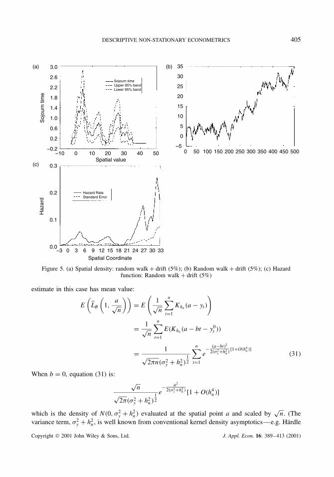
Figure 5. (a) Spatial density: random walk C drift (5%); (b) Random walk C drift (5%); (c) Hazardfunction: Random walk C drift (5%)

estimate in this case has mean value:

E

(LB

(1,

apn

))D E

(1pn

n∑tD1

Khna � yt�

)

D 1pn

n∑tD1

EKhna � bt � y0t ��

D 1p

2�n�2y C h2

n�12

n∑tD1

e� a�bt�2

2�2yCh2

n�[1COh4

n�]31�

When b D 0, equation (31) is:pn

p2��2

y C h2n�

12

e� a2

2�2yCh2

n� [1 C Oh4n�]

which is the density of N0, �2y C h2

n� evaluated at the spatial point a and scaled bypn. (The

variance term, �2y C h2

n, is well known from conventional kernel density asymptotics—e.g. Hardle



and Linton, 1994). When b 6D 0, equation (31) can be approximated for large n by writingbt ¾ bn0t/n� where n0 < n is large and fixed. Then, (31) is approximately:

1p

2�n�2y C h2

n�12

n∑tD1

e�

a�bn0tn �2

2�2yCh2

n�[1COh4

n�] ¾pn

p2��2

y C h2n�

12

∫ 1

0e

� a�bn0r�2

2�2yCh2

n�[1COh4

n�]dr

Dpn

jbjn032�

which we note to be independent of the spatial point a. Thus, in the trend stationary case, thespatial density estimate has approximately constant mean, corroborating the form of the empiricalestimate found in Figure 4. Thus, one of the characteristics of spatial densities of trend stationaryseries is that that the mean density is approximately constant over the support. As we will see,this behaviour is quite different from the spatial density of a random walk with drift.

Figure 5 gives the spatial density of a random walk with a 5% drift, so that the deterministiccomponent here is the same as it is in the trend stationary case. It is apparent from Figure 5(a)that the regions [3, 5] and [23, 27] are the most frequently visited in this sample path. Clearly, thespatial support is far wider than in the case of no drift (Figure 2), but the curve is just as irregular.

This can be explained by noting that if Mr� D br C Br� is Brownian motion with drift, thendM D bdr C dB, so that dM�2 D dB�2 D dt and the quadratic variation process of M is the sameas that of B, i.e. [M]t D [B]t D ∫ t

0 dB�2. Then:

LMr, s� D limε!0

1

2ε

∫ r

01jMt� � sj < ε� d[M]t

D limε!0

1

2ε

∫ r

01jBt� � s � bt�j < ε� dt

and the sojourn time of M at s can be regarded as a version of the sojourn time of Brownianmotion recentred around the drift.

Finally, we compute the hazard functions for the trend stationary and difference sta-tionary data shown in Figure 4(b) and 5(b). The hazard function for the trend stationarydata is shown in Figure 4(c). According to (32), we would expect the hazard rate for(what is on average, at least) a uniform density to be a steadily increasing function, andFigure 4(c) shows this to be approximately so. On the other hand, for the difference sta-tionary data, as is apparent from the spatial density estimate given in Figure 5(b), thereare regions of greater spatial concentration around 3–5, 13–15 and 25–27. These regionsshow up as peaks in the hazard function shown in Figure 5(c). All these peaks appearsignificant. In both Figures 4(c) and 5(c) the standard errors rise with the spatial coordi-nate and ultimately the hazard estimates become unreliable as the data thins out in theright tail.

4. EMPIRICAL APPLICATIONS

4.1. Exchange Rate Data and Target Zones

Exchange rate data under floating regimes typically behave as if they have no fixed mean and areusually well represented by unit root processes. Intermediate between fixed and flexible exchange



rate regimes are target zone systems where exchange rates are permitted to float within bands.This exchange rate mechanism was operated by the European Monetary System (EMS) over the1980s and 1990s. For most countries in the EMS, the bands were set at š2.25% around a centralparity that was occasionally adjusted by currency realignments. Such exchange rate target zoneshave been the subject of considerable research. A theory model for exchange rate target zones wasdeveloped by Krugman (1991, 1992) and has formed the starting point in much of the subsequentresearch on this topic. This model allows for the determination of the exchange rate within the bandin terms of a non-linear function of economic fundamentals which are represented by Brownianmotion. The non-linear function arises because of the presence of monetary policy interventiondesigned to keep the exchange rate in the band. It has an S-curve shape and approaches the edgeof the band in a smooth tangential fashion that is characterized as ‘smooth pasting’ (Dixit, 1993).One of the empirical implications of this theory is that the distribution of exchange rates withinthe band should be U-shaped, so that there is, in effect, a greater concentration of observationscloser to the edge of the band than in the center of the band.

The empirical evidence in support of this implication of the target zone model can be assessedby using our spatial density approach. Figure 6(b) shows the French Franc/German mark exchangerate from March 1979 through to March 1992 in terms of deviations from the central parity atthe beginning of the period. This data was used by Svensson (1992) in his review of the targetzone literature. The š2.25% bands around the central parity are shown by broken lines in thisfigure. Successive realignments in the central parity are also shown, occurring in September 1979,October 1981, June 1982, March 1983, April 1986 and January 1987. All these realignmentsdevalued the franc against the mark.

Combining these periods together by subtracting the central parity in each period, we may focuson the behaviour of the exchange rates within the bands, which was Krugman’s (1991) concern,and ignore issues of jumps in the bands themselves, which is a different issue that has attractedsubsequent attention (e.g. Pesaran and Ruge-Murcia, 1999). Figure 6(c) shows this transformeddata and Figure 6(a) gives the spatial density for this data. The figure shows strong evidence ofbimodality in the data, revealing a clear peak in spatial density at the lower edge of the bandaround �2%. The remainder of the data appears to be spread out fairly evenly over the positiveregion of the band [0, 2.25]. These results provide partial support for the conclusion from thetarget zone model that exchange rates should tend to cluster near the edges of the band. However,the spatial density is clearly not U-shaped, and there appears to be a strong tendency in thesedata for the exchange rate to spend a good deal of time in the centre of the band as well asnear the edges, a feature that is also fairly evident in the time plot of the data. What the spatialdensity in Figure 6(a) adds to a close examination of the time plot of the data is a quantitativeevaluation of the relative importance of different spatial locations, precisely the matter that needsto be addressed in considering the empirical implications of the target zone theory model. Thus,while the target zone model is rejected, it appears that there are some implications of the modelthat do find support in the data.

4.2. Inflation Data: Measuring Inflation and Deflation Hazards

Figure 7(a) shows annual CPI inflation rates for the USA based on monthly data for the CPI overthe period 1934:1–1997:12. The time plot shows several periods of two-digit inflation, periodsof deflation and substantial volatility in inflation, especially at higher rates. Figure 7(b) gives the



0.8

0.7

0.6

0.5

0.4

0.3

–3 –2 –1Exchange Rate: % change from Central Parity

0 1 2 3 4 5

0.2

0.1

0.0

Soj

ourn

tim

e Sojourn timeUpper 95% bandLower 95% band

–0.1 –0.05

0.00

0.05

0.10

0.15

0.20

0.25

0.30

0.35

0.40

0.45

80 81 82 83 84 85 86 87 88 89 90 91 92 93 94

% fr

om M

arch

197

9 P

arity

–0.02

–0.03

–0.01

0.00

0.01

0.02

0.03

80 81 82 83 84 85 86 87 88 89 90 91 92 93 94

% fr

om C

entr

al P

arity

(a)

(c)

(b)

Figure 6. (a) Spatial density of FF/DM exchange rate; (b) FF/DM exchange rate data; (c) FF/DM dataabout central parity

spatial density estimate and reveals a primary concentration of variation around the 16% inflationrate, a mode around 9% inflation and a further mode indicating a peak in deflation around �2.5%.

Figure 7(c) gives hazard rate estimates for US inflation. Inflation hazards clearly peak at lowlevels (around 3%), intermediate levels (around 6%) and low two-digit levels (around 10–12%).The 3% and 10–12% peaks are both statistically significant and there is a fall-off in the hazard ratearound 8%, between the peaks. The rising hazard around 16% is insignificant and can be ignored,being dependent on only a few observations. Overall, these estimates indicate that, conditional onthere being inflation, historical experience over the last 60 years in the USA indicates that thepredominant inflation risks are at low levels and low two-digit levels.

Figure 7(d) gives hazard rate estimates for US deflation. These are based on an estimate of theleft-sided hazard function (21). The unbroken line in Figure 7(d) measures the conditional risk ofinflation at a particular rate, given that inflation is no greater than that particular rate. Thus, whenthat inflation rate is negative, the curve measures the conditional risk of deflation. The estimates



Hazard RateStandard error

1.0

0.9

0.8

0.7

0.6

0.5

0.4

0.3

0.2

0.1

0.0–4.0 –3.0 –2.0 –1.0 0.0

Inflation rate1.0 2.0 3.0 4.0

Haz

ard

Hazard RateStandard error

0.3

0.2

0.1

0.0–4 –2 0 2 4 6 8 10 12 14 16 18

Inflation rate

Haz

ard


3.5

3.0

2.5

2.0

1.5

1.0

0.5

0.0

–0.5–10 –6 –2 2 6

Inflation rate10 14 18 22

Soj

ourn

Tim

e

18

12

9

6

3

0

15

–3

–637 41 45 49 53 57 61 65 69 73 77 81 85 89 93 97

Infla

tion

rate

(a)

(c) (d)

(b)

Figure 7. (a) US inflation 1934–97; (b) Spatial density of US inflation 1934–97; (c) US inflation hazard1934–37; (d) US deflation hazard 1934–97

shown in Figure 7(d) indicate that there is a significant risk of deflation around the �1% level.The risk then falls off and subsequently rises again to another peak around �3.5%. This peak andthe subsequent higher rates of deflationary risk are statistically insignificant and are based on onlya single episode of high deflationary rates experienced in the interwar period. In sum, we maytake these estimates as indicative of a non-negligible risk of low levels of deflation (around �1%)based on historical US experience.

4.3. Opinion Poll Data: Nixon and Clinton Approval Ratings

We end this empirical section with a brief application to political opinion poll data. Like manyeconomic time series, there is substantial evidence that presidential opinion poll data are wellmodelled by unit root processes (e.g. Blood and Phillips, 1995, 1997). As such, this type of data isamenable to the type of descriptive statistical analysis considered in this paper. In some respects,our approach is particularly useful with data of this type because the data is usually not equallyspaced in time, making conventional discrete time modeling difficult. Figures 8(b) and 9(b) show



1.4

1.0

0.6

Soj

ourn

tim

e

App

rova

l Rat

ing

%

0.2

–0.2 20 30 40 50 60

Popularity level %

70 80

75

70

65

60

55

50

45

40

35

30

25

2069 70 71 72 73 74 75


(a) (b)

Figure 8. (a) Spatial density of Nixon approval ratings; (b) President Nixon approval ratings

1.4

1.0

0.6

Soj

ourn

tim

e

App

rova

l Rat

ing

%

0.2

–0.230 40 50

Popularity level %

60 70

66

62

58

54

50

46

42

38

3493 94 95 96 97 98


(a) (b)

Figure 9. (a) Spatial density of Clinton approval ratings; (b) President Clinton approval ratings

opinion poll data for the Nixon and Clinton presidencies. From these data, the spatial densitieswere computed and are shown in Figures 8(a) and 9(a).

As is apparent from the time plot of the data in Figure 8(b), the latter part of the Nixon presidencywas characterized by a sharp falling off in the ratings as the Watergate crisis culminated. Forobvious reasons, Nixon approval ratings do not follow a stationary process. Nevertheless, we mayconduct a spatial density analysis along the lines we have discussed. The spatial density estimateshown in Figure 8(a) manifests the phenomenon of the effects of the fulminating Watergate crisison the Nixon presidency in a remarkably clear bimodality in the Nixon approval ratings, with asignificant lower mode in approval around 25%.

Figure 9(b) gives a time plot of the approval ratings for President Clinton, up to November 1997,prior to the breaking of the Lewinski scandal. The spatial density of Clinton approval ratings are



shown in Figure 9(a). Apparently, it is hard to reject that Clinton approval ratings are uniformlydistributed over the region [40%, 60%], indicating a clear difference in the spatial distributionof approval ratings between the two presidencies. Obviously, it will be of interest to use thesemethods to assess the effects of the Lewinski scandal on the spatial distribution of Clinton approvalratings.

5. CONCLUDING COMMENTS ON THE RELATION TO NON-PARAMETRIC METHODS

Econometric work, like other applications of statistics, involves data reduction. Even descriptivetechniques, like the spatial densities and hazard rates that are applied here, necessitate a loss ofinformation. Their usefulness comes from the need to discover regular features of the data andconvenient means of expression for them, tasks that seems to be much more difficult for non-stationary data than they do for stationary data. However, while we no longer have a framework oftime-invariant characteristics to rely upon when the data are non-stationary, we can find convenientquantitative representations of their sample characteristics without being dependent on the use ofa specific model. Thus, whereas we no longer have fixed population moments or a time-invariantprobability density to rely upon, we do have a well-defined concept of spatial location that hasmeaning beyond the immediate sample data. Our analysis shows that it is possible to constructquantitative measures of spatial density and apply these measures in an informative way to avariety of different data sets. Once this has been done, it is possible to use these measures in furtherconstructive ways to estimate interesting functionals of spatial densities like hazard functions.

The techniques discussed and illustrated in this paper have a certain role to play in the ongoingevolution of econometric methods. In recent years, much of econometrics has been concernedwith an attempt to achieve generality wherever possible, without sacrificing specificity where itconnects most closely to underlying economic ideas. One way of attaining generality that hasbecome increasingly popular in both microeconometric and time series studies is the use of non-parametric and semiparametric techniques. These techniques seek to avoid precise formulationsor specific functional representations wherever generality is considered desirable and, thereby, itis hoped that the techniques will sit more comfortably with abstract propositions of economictheory. Nevertheless, existing validation of the use of these techniques has rested on the presenceof invariant functional quantities, like a probability density or a spectrum, that can be estimated.What the methods of this paper show is that the notion of a general non-parametric approach todata analysis continues to retain validity even when the data are manifestly non-stationary andthere are no underlying time-invariant quantities to estimate. What changes is not the approach todata analysis, but the interpretation of the empirical quantities that emerge from a non-parametricanalysis. For non-stationary series, these quantities simply reflect variational decompositions acrossspace rather than probability decompositions.

6. NOTATION

!a.s almost sure convergence!p convergence in probabilityDd distributional equivalenceBr� Brownian motionBM�2� Brownian motion with variance �2



1A� indicator of AMN (0, G) mixed normal distribution with mixing variate G), !d weak convergence[Ð] integer part ofr ^ s min(r, s)� equivalenceop1� tends to zero in probabilityoa.s.1� tends to zero almost surely

ACKNOWLEDGEMENTS

Some of the methods and empirical results given here were first reported in one of the author’sJournal of Applied Econometrics Annual Lectures at the University of Wisconsin in April 1998.Thanks go to the Department of Economics at the University of Wisconsin for hosting theselectures and to the JAE for extending the invitation to present them. The author thanks Zhian-HuaZhu for supplying the opinion poll data, and Alex Maynard for help in obtaining the exchangerate data. Thanks also go to the NSF for research support under Grant Nos, SES 94-22922 andSBR-9730295. The computations were performed by the author in GAUSS.

REFERENCES

Blood DJ, Phillips PCB. 1995. Recession headlines, consumer sentiment, the state of the economy andpresidential popularity: A time series analysis 1989–1993. International Journal of Public OpinionResearch 7: 2–22.

Blood DJ, Phillips PCB. 1997. Economic headline news on the agenda: new approaches to understandingcauses and effects. In Communication and Democracy: Exploring the Intellectual Frontiers in Agenda-Setting Theory, McCombs M, Shaw DL, Weaver D (eds). Lawrence Erlbaum: London.

Bosq D. 1998. Nonparametric Statistics for Stochastic Processes (2nd edn). Springer: New York.Csorgo M, Horvath L. 1993. Weighted Approximations in Probability and Statistics. Wiley: New York.Dixit A. 1993. The Art of Smooth Pasting. Harwood Academic Publishers: Chur.Espasa A, Sargan JD. 1977. The spectral estimation of simultaneous equation systems with lagged endoge-

neous variables. International Economic Review 18: 583–605.Feller W. 1957. An Introduction to Probability Theory and its Applications (Vol. I, 2nd edn). Wiley: New

York.Hannan EJ. 1963. Regression for time series. In Time Series Analysis, Rosenblatt M (ed.). Wiley: New York;

17–37.Hardle W, Linton O. 1994. Applied nonparametric methods. In The Handbook of Econometrics (Vol. IV),

McFadden DF, Eagle RF III (eds). North-Holland: Amsterdam.Krugman P. 1991. Target zones and exchange rate dynamics. Quarterly Journal of Economics 106: 669–682.Krugman P. 1992. Exchange rates in a currency band: a sketch of the new approach. In Exchange Rate

Targets and Currency Bands, Krugman P, Miller M (eds). Cambridge University Press: Cambridge.Pesaran MH, Ruge-Murcia FJ. 1999. Analysis of exchange-rate target zones using a limited dependent

rational expectations model with jumps. Journal of Business and Economic Statistics 17: 50–66.Phillips PCB. 1986. Understanding spurious regressions in econometrics. Journal of Econometrics 33:

311–340.Phillips PCB. 1987. Time series regression with a unit root. Econometrica 55: 277–301.Phillips PCB. 1988. Multiple regression with integrated processes. In Statistical Inference from Stochastic

Processes, Contemporary Mathematics, Prabha NV (ed.). 80: 79–106.Phillips PCB. 1998a. Econometric analysis of Fisher’s equation. Cowles Foundation Discussion Paper, No.

1180. Yale University.



Phillips PCB. 1998b. New tools for understanding spurious regressions. Econometrica 66: 1299–1326.Phillips, Solo. 1992. Asymptotics for Linear processes. Annals of Statistics 20: 971–1001.Phillips PCB, Park JY. 1998. Nonstationary density estimation and kernel autoregression. Cowles Foundation

Discussion Paper No. 1181, Yale University.Revuz D, Yor M. 1994. Continuous Martingales and Brownian Motion (2nd edn). Springer-Verlag: New

York.Sargan JD. 1953. An approximate treatment of the properties of the correlogram and peridogram. Journal of

the Royal Statistical Society, Series B 15: 140–152.Sargan JD. 1958. The estimation of economic relationships using instrumental variables. Econometrica 26:

393–415.Sargan JD. 1959. The estimation of relationships with autocorrelated residuals by the use of the instrumental

variables. Journal of the Royal Statistical Society, Series B 21: 91–105.Silverman BW. 1986. Density Estimation for Statistics and Data Analysis. Chapman and Hall: London.Sims CA. 1980. Macroeconomics and reality. Econometrica 48: 1–48.Svensson LEO. 1992. An interpretation of recent research on exchange rate target zones. Journal of Economic

Perspectives 6: 119–144.Tyurin K, Phillips PCB. 1999. The occupation density of fractional Brownian motion and some of its

applications. Yale University, mimeo.Geman D, Horowitz J. 1980. Occupation densities. Annals of Probability 8: 1–67.


descriptive econometrics for non-stationary time series - the cowles

Documents