description and control of decoherence in quantum bit systems · pdf filedescription and...
TRANSCRIPT

Description and control of decoherencein quantum bit systems
Henryk Peter Gregor Gutmann
Munchen, Juni 2005


Description and control of decoherencein quantum bit systems
Henryk Peter Gregor Gutmann
Dissertation
an der Fakultat fur Physik
der Ludwig–Maximilians–Universitat
Munchen
vorgelegt von
Henryk Peter Gregor Gutmann
aus Bonn
Munchen, Juni 2005

Erstgutachter: PD Frank K. Wilhelm
Zweitgutachter: Prof. Dr. Axel Schenzle
Tag der mundlichen Prufung: 03.08.2005
Contents
List of Publications ix0.1 Introduction . . . . . . . . . . . . . . . . . . . . . . . . . . . . . . . . . . . 1
0.1.1 Outline of the thesis . . . . . . . . . . . . . . . . . . . . . . . . . . 3
1 Derivation of Lindblad type master equations at finite temperatures 71.1 Introduction . . . . . . . . . . . . . . . . . . . . . . . . . . . . . . . . . . . 71.2 Lindblad equation in the Bloch sphere representation . . . . . . . . . . . . 10
1.2.1 Lindblad requirements and the concept of dynamical semigroups . . 101.2.2 GKS formulation of the Lindblad equation . . . . . . . . . . . . . . 121.2.3 Bloch-sphere formalism . . . . . . . . . . . . . . . . . . . . . . . . . 13
1.3 Born-Markov master equations . . . . . . . . . . . . . . . . . . . . . . . . 141.3.1 Born approximation . . . . . . . . . . . . . . . . . . . . . . . . . . 141.3.2 Markov approximations . . . . . . . . . . . . . . . . . . . . . . . . 17
1.4 Spin-Boson Hamiltonian . . . . . . . . . . . . . . . . . . . . . . . . . . . . 241.4.1 Thermodynamic limit and Ohmic bath . . . . . . . . . . . . . . . . 25
1.5 Numerical results . . . . . . . . . . . . . . . . . . . . . . . . . . . . . . . . 271.5.1 Naıve Markov approximation . . . . . . . . . . . . . . . . . . . . . 271.5.2 Davies- Luczka approximation . . . . . . . . . . . . . . . . . . . . . 281.5.3 Bloch-Redfield approximation . . . . . . . . . . . . . . . . . . . . . 281.5.4 Celio-Loss approximation . . . . . . . . . . . . . . . . . . . . . . . 29
1.6 Quantitative comparison of the Born-Markovian approximations . . . . . . 301.7 summary . . . . . . . . . . . . . . . . . . . . . . . . . . . . . . . . . . . . . 34
2 Qubit decoherence due to bistable fluctuators 352.1 Qubit-bfl-bath model . . . . . . . . . . . . . . . . . . . . . . . . . . . . . . 372.2 Bloch-Redfield master equation . . . . . . . . . . . . . . . . . . . . . . . . 39
2.2.1 Bloch-Redfield tensor . . . . . . . . . . . . . . . . . . . . . . . . . . 392.2.2 Qubit dephasing and relaxation rates . . . . . . . . . . . . . . . . . 402.2.3 Qubit decoherence spectra at fixed Ωq for variable T . . . . . . . . 412.2.4 Qubit decoherence spectra at fixed T for variable Ωq . . . . . . . . 432.2.5 1/f noise . . . . . . . . . . . . . . . . . . . . . . . . . . . . . . . . 46
2.3 Stochastic Schrodinger equation and random walk model . . . . . . . . . . 482.3.1 Stochastic Hamiltonian . . . . . . . . . . . . . . . . . . . . . . . . . 49

vi CONTENTS
2.3.2 Random walk model . . . . . . . . . . . . . . . . . . . . . . . . . . 51
2.3.3 Symmetrical noise . . . . . . . . . . . . . . . . . . . . . . . . . . . . 55
2.3.4 Bfl-noise at finite temperatures . . . . . . . . . . . . . . . . . . . . 56
2.3.5 Criteria for an appropriate choice of bfl parameter . . . . . . . . . . 59
2.3.6 Numerical and analytical results for temperature dependent bfl noise 61
2.3.7 Derivation of dephasing and relaxation rates . . . . . . . . . . . . . 64
2.4 Bfl-noise induced by an SET-measurement setup . . . . . . . . . . . . . . . 67
2.4.1 Flipping rates of the SET-electron . . . . . . . . . . . . . . . . . . . 68
2.5 Refocusing of bfl-noise by means of dynamical decoupling . . . . . . . . . . 73
2.5.1 Refocusing (bang-bang) scheme . . . . . . . . . . . . . . . . . . . . 74
2.5.2 Random walk model . . . . . . . . . . . . . . . . . . . . . . . . . . 75
2.5.3 Pulse shapes . . . . . . . . . . . . . . . . . . . . . . . . . . . . . . . 78
2.5.4 Distributions of the random walks deviation . . . . . . . . . . . . . 79
2.5.5 Bang-bang control working as a high-pass filter . . . . . . . . . . . 80
2.5.6 Bang-bang refocusing of finite temperature bfl-noise . . . . . . . . . 82
2.5.7 Applicability of imperfect bang-bang pulses . . . . . . . . . . . . . 85
2.5.8 Numerical and analytical results . . . . . . . . . . . . . . . . . . . . 87
3 Quantum phase diagram of a coupled qubit system 93
3.1 The 2-spins-3-bosonic-baths model . . . . . . . . . . . . . . . . . . . . . . 93
3.2 The dressed double-spin Hamiltonian . . . . . . . . . . . . . . . . . . . . . 96
3.2.1 The Emery-Kivelson-transformation . . . . . . . . . . . . . . . . . . 97
3.3 Scaling analysis and quantum phase diagram . . . . . . . . . . . . . . . . . 100
3.3.1 Scaling equations 1st order . . . . . . . . . . . . . . . . . . . . . . . 100
3.3.2 Entanglement capability of the fixed point Hamiltonian . . . . . . . 102
3.4 Scaling equations 2nd order . . . . . . . . . . . . . . . . . . . . . . . . . . . 105
3.4.1 Operator product expansion . . . . . . . . . . . . . . . . . . . . . . 105
A Born master equation of the spin-Boson model 109
A.1 Derivation of the Born approximation correlation functions . . . . . . . . . 109
B Born-Markovian approximations of the Spin-Boson model 113
B.1 Naıve Markov approximation . . . . . . . . . . . . . . . . . . . . . . . . . 113
B.2 Bloch-Redfield approximation . . . . . . . . . . . . . . . . . . . . . . . . . 120
B.3 Davies- Luczka approximation . . . . . . . . . . . . . . . . . . . . . . . . . 124
B.4 Lindblad approximation according Celio and Loss . . . . . . . . . . . . . . 129
C Random walk analysis 131
C.1 Symmetrical random walk (driftless) . . . . . . . . . . . . . . . . . . . . . 131
C.1.1 Pure bfl-noise . . . . . . . . . . . . . . . . . . . . . . . . . . . . . . 131
C.1.2 Bang-bang refocused random walk . . . . . . . . . . . . . . . . . . 133

Table of Contents vii
D Bosonic fields scaling formalism 135D.1 Derivation of the first order scaling equations . . . . . . . . . . . . . . . . 135D.2 Derivation of the second order scaling equations . . . . . . . . . . . . . . . 136
D.2.1 Calculation of the operator product expansions . . . . . . . . . . . . 137
Acknowledgements 154
Deutsche Zusammenfassung 160

viii Table of Contents

List of Publications
Major parts of this thesis are discussed in the following publications
chapter 1
1. Derivation of Lindblad type master equations by means ofBorn Markov approximations at finite temperatureHenryk Gutmann and Frank K. Wilhelmin preparation.
chapter 2
2. Bang-bang refocusing of a qubit exposed to telegraph noiseHenryk Gutmann, F.K. Wilhelm, W.M. Kaminsky and S. LloydQuantum Information Processing 3, 247 (2004).
3. Compensation of decoherence from telegraph noise by means ofan open loop quantum-control techniqueHenryk Gutmann, W.M. Kaminsky, Seth Lloyd and Frank K. WilhelmPhysical Review A 71, 020302 (2005).
4. Dynamical decoupling of bistable fluctuator noise at finite temperatureHenryk Gutmann, A. Holzner, F.K. Wilhelm, W.M. Kaminsky and S. Lloydin preparation.
5. Random Walk description of backaction during quantum charge detectionHenryk Gutmann, A. Holzner and F.K. Wilhelmin preparation.
chapter 3
6. Scaling analysis of a coupled two-spin system exposed tocollective and localized noiseHenryk Gutmann, Gergely Zarand and Frank K. Wilhelmin preparation.

x Introduction

List of Figures
1.1 Davies- Luczka permutation of the integration order . . . . . . . . . . . . . 211.2 Qubit-bath model . . . . . . . . . . . . . . . . . . . . . . . . . . . . . . . . 241.3 GKS eigenvalues for the naıve Markovian and Davies- Luczka approximation 281.4 GKS eigenvalues for the Bloch-Redfield and Celio-Loss approximation . . . 291.5 Evolution of the spin-Boson model in Born approximation . . . . . . . . . 311.6 Evolution of the spin-Boson model in Markovian approximations . . . . . . 321.7 Fidelity and coherence decay of Born Markovian evolutions . . . . . . . . . 33
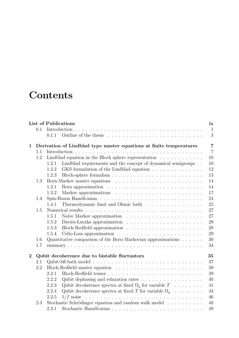
2.1 Qubit-bistable fluctuator-heat bath model . . . . . . . . . . . . . . . . . . 372.2 Qubit relaxation rates at variable temperatures and Ωbfl . . . . . . . . . . 412.3 Peak positions of the qubit-bfl resonance spectra of relaxation rates . . . . 422.4 Qubit relaxation rates at variable Ωbfl and fixed temperature T = 0.05K . 432.5 Qubit relaxation rates at variable Ωbfl and fixed temperature T = 0.5K . . 442.6 Peak positions of the qubit-bfl resonance spectra of relaxation rates . . . . 452.7 Peak heights of the qubit-bfl resonance spectra of relaxation rates . . . . . 452.8 1/f type relaxation rate behaviour . . . . . . . . . . . . . . . . . . . . . . 462.9 Crossover 1/f to 1/f 2 type relaxation rate behaviour . . . . . . . . . . . . 472.10 Telegraph noise due to bfl . . . . . . . . . . . . . . . . . . . . . . . . . . . 492.11 Bfl induced random walk on the Bloch sphere . . . . . . . . . . . . . . . . 512.12 One-step random walk deviation due to bfl noise . . . . . . . . . . . . . . . 522.13 Evolution of the bfl random walk deviation . . . . . . . . . . . . . . . . . . 562.14 Asymmetric bfl noise . . . . . . . . . . . . . . . . . . . . . . . . . . . . . . 582.15 Temperature dependence of bfl flipping times . . . . . . . . . . . . . . . . . 612.16 Random walk evolutions of temperature dependent bfl noise . . . . . . . . 622.17 Random walk deviations of temperature dependent bfl noise . . . . . . . . 632.18 Dephasing on the Bloch sphere . . . . . . . . . . . . . . . . . . . . . . . . 642.19 Relaxation on the Bloch sphere . . . . . . . . . . . . . . . . . . . . . . . . 652.20 Physical setup of an SET-SCB measurement design . . . . . . . . . . . . . 672.21 Level structure of an SET . . . . . . . . . . . . . . . . . . . . . . . . . . . 692.22 Decoherence of SET induced bfl noise . . . . . . . . . . . . . . . . . . . . . 702.23 Temperature dependence of flipping times of an SET . . . . . . . . . . . . 712.24 Dephasing and relaxation times due to SET noise . . . . . . . . . . . . . . 722.25 Bang-bang refocusing of bfl induced random walk . . . . . . . . . . . . . . 73

xii List of Figures
2.26 Detailed plot of bang-bang refocused bfl noise . . . . . . . . . . . . . . . . 742.27 One-step random walk deviation of bang-bang refocused bfl noise . . . . . 762.28 Random walk evolution of bfl noise with and without bang-bang control . . 772.29 Two-step random walk distributions of sudden and smooth bang-bang pulses 782.30 Distributions of pure and bang-bang refocused bfl induced random walk . . 792.31 Bang-bang suppression factor . . . . . . . . . . . . . . . . . . . . . . . . . 802.32 Temperature dependence of bang-bang refocused bfl noise (1) . . . . . . . 822.33 Temperature dependence of bang-bang refocused bfl noise (2) . . . . . . . 832.34 Suppression factors as function of bang-bang times . . . . . . . . . . . . . 842.35 Suppression factors as function of temperature . . . . . . . . . . . . . . . . 852.36 Dephasing aberrations due to faulty bang-bang pulses . . . . . . . . . . . . 862.37 Relaxating aberrations due to faulty bang-bang pulses . . . . . . . . . . . . 882.38 Random walk deviations due to faulty bang-bang pulses . . . . . . . . . . 892.39 Random walk deviations due to faulty bang-bang refocused bfl noise . . . . 90
3.1 Figure of the 2-spin-3-Bosonic baths model . . . . . . . . . . . . . . . . . . 943.2 Physical realization of the 2-spin-3-Bosonic baths model . . . . . . . . . . . 953.3 Quantum phase diagram by means of scaling analysis 1st order . . . . . . . 101
A.1 Exponential decay of the Born correlation functions . . . . . . . . . . . . . 111

0.1 Introduction 1
calvinandhobbes c©2005.Watterson.reprinted-by-permission-of-universal-press-syndicate.allrights-reserved
0.1 Introduction
In the last decade quantum computing and information methods have become a field of in-terest of strong prominence for various experimental and theoretical disciplines [1, 2, 3, 4].Besides its practical relevance for solving mathematically and computationally hard prob-lems, in particular the breaking of current decryption techniques, this is founded in theunique combination of fundamental research of quantum mechanics with modern experi-mental methods. This renaissance of an original idea by Richard Feynman [5] in practisehas led to many successful results in mesoscopic setups. Which includes e.g. the obser-vation of interference phenomena in Rabi and Ramsey type experiments [6, 7], as well ascontinuous increase of decoherence times as a consequence of more effective shielding, cool-ing and e.g. cleaner fabrication of the mesoscopic setups, quantum information is storedand computed on. Also the feasibility of two-qubit gates have been experimentally provenin various realizations [8].
On the other hand theoretical developments have made the implementation of a quan-tum computing device more probable. In particular there is a threshold quality for quantumgates, i.e. a maximum error rate at the order of 10−4, under which arbitrary long quan-tum computing should be feasible by means of appropriate error correction techniques[9, 2]. The application of encoding methods used to construct so-called decoherence freesubspaces [10, 11], enlarges the confidence that quantum computing in principle could beimplemented in spite of the omnipresent decoherence, which makes it such an expensivetechnical challenge. Last but not least, one should also quote alternative approaches ase.g. adiabatic quantum computation [12], which promises to provides beneficial resultseven in strongly correlated and quite non-coherent systems, at least for a particular classof mathematical problems.
David DiVincenzo has tabulated a catalogue of physical criteria, which in general shouldbe fulfilled for experimental approaches to be promising candidates as future quantumcomputing devices [13]. This list of DiVincenzo criteria, lately extended by the concept of

2 List of Figures
“flying qubits” (the demand of the ability to exchange quantum information between dif-ferent quantum computing devices, quasi the potentiality to build up networks of qubits),provides a guideline for any physical setup. It serves to decide, how close a physical setup isto a possible realization of quantum computation and to specify, where the remaining mainproblems lie. In accordance with this criteria, a US government panel recently laid out a“road-map”[14], where is listed, which of the DiVincenzo criteria have been or should befulfilled in close future, regarding the various physical approaches. Of course, that reportof actual and future status is updated from time to time.
There are different approaches for realizing quantum bits. At first should be mentionedthe nuclear-magnetic resonance technique (NMR) [15] being the oldest and most developedmethod, which originally was invented for spin spectroscopy. Thereby different resonancesof specified nuclear spins in appropriate designed molecules can be used as carrier of quan-tum information. As these spins couple only extremely weakly to the environment (whichleads to extremely long decoherence times), one has to use huge ensembles (in typicalmacroscopic order of numbers ' 1023) and apply very strong magnetic fields on the NMRprobes. Nevertheless, the most powerful implementation, liquid state NMR, can be refinedat room temperature and although NMR is working almost with thermal equilibrium statesthere have been invented numerous techniques to circumvent most NMR drawbacks. Inparticular by means of NMR technique the factorization of 15 [16] has been accomplished.Its non-scalability in larger sizes of qubit registers is probably a crucial reason for discard-ing NMR techniques for a future quantum computer.
Good results regarding decoherence times and experiences in manipulation of quantumbits as well have been achieved by quantum optics methods [17, 18]. The qubit is therebydefined as two levels of a particular atomic or molecular excitation process, respectivelydefined by two specific states of a photonic or microwave cavity. Rabi and Ramsey type ex-periments have proven compareably impressive decoherence times, as well as the capabilityto exchange of quantum information [7]. The method of ion traps and optical lattices arequite related to that field [19, 20]. Quantum information is stored in atomic or molecularenergy levels as well and quantum manipulation and read-out are also performed by opticaltechniques, e.g. by means of laser pulses.
Probably the most promising approaches at least with respect to the yet unsolvedproblem of scalability provides the electric circuit implementations based on semi- and/orsuperconductor technology. On the one semi-conductor side there are quantum dot tech-niques where an appropriate confined restriction of two-dimensional electron gases leads toan artificial atomic level structure easy to manipulate electro-statically by correspondinggate voltages. These discrete level structures can be used to provides well-defined qubits,which can be manipulated electro-statically or by means of magnetic fields [21, 22]. Onthe other (superconducting) hand, Josephson junctions assembled in electric circuits pro-vides us with mesoscopic effective two-level systems, which can be based on persistentcurrents (leading to so-called Josephson flux qubits) or on electron charges confined on

0.1 Introduction 3
zero-dimensional islands (thus similar to quantum dot realizations) [23, 24, 25, 26, 27].
While different realizations have their characteristic advantages and drawbacks, thesemi- and superconducting approaches probably provide the most promising candidates forreal large-scaled quantum registers, as mesoscopic electrical circuit techniques are most ob-vious in regard of enlargening the corresponding quantum registers. Moreover, productiontechniques for computational electrical circuits have gained experiences in miniaturizingand perfecting their devices for almost half a century.
From the theoretical point of view it would be a desireable goal to derive a general for-malism describing any kind of mesoscopic realization of qubit registers as well as the uponapplied quantum gates including the miscellaneous influences of decoherence. There existdifferent approaches; at first master equations as kinetic equations of the density matricespresenting the (decohering) quantum states of the qubit registers. There are basically twoways of deriving them. Either by a phenomenological approach (which in particular is theusual way for deriving Lindblad type master equations). Or by applying perturbation the-ory, which is often a good choice if the environmental couplings were appropriately weak,as they define the perturbative parameter.
Quantum Langevin equations as for instance stochastic Schrodinger equations, canalso provides a useful formalism. There the environmental noise is usually introduced bystochastic perturbation in the corresponding Schrodinger equations. For certain cases,there exist one-to-one mappings between master equations and corresponding stochasticSchrodinger equations, also denoted quantum state diffusion ([28] and references therein).For strongly coupled systems, where usual perturbation theory fails, are numerical tech-niques preferred ([29, 15, 30]). But these cases are not the most relevant for usual quantumbit realizations, as strong coupling to the environment normally means stronger decoher-ence and therefore less capability of storing and processing quantum information. Oneexception could be adiabatic quantum computing, where decoherence times do not neces-sarily play a crucial role.
Nevertheless, we will discuss a qualitative scheme of estimating effective quantum dy-namics of a coupled two spin system exposed to arbitrary strong bath coupling. In partic-ular we will find evidences for the presence of entanglement (i.e. the spatially non-localityof quantum information, which besides quantum coherence makes quantum computing de-vices so powerful).
0.1.1 Outline of the thesis
In our first chapter we will propose several attempts to derive Lindblad type master equa-tions by use of perturbation theory on microscopic models. We quote an easily applicablecriterion to decide whether a given Markovian master equation possesses the Lindblad form

4 List of Figures
or not. As exemplaric and highly relevant qubit decoherence model, we consider therebythe spin-Boson model with Ohmic heat bath spectral density. We conclude the first chapterwith some quantitative comparisons of the fidelity between the various Markov approxi-mations.
After the primarily formal discussion of master equations properties, presenting distur-bances generated from Gaussian noise sources, i.e. where the central limit theorem applies,we will focus on a different class of noise sources, the so-called bistable fluctuators. TheseNevertheless seems to be a very universal problem, in particular for condensed matter re-alizations. Thereby we will apply three different models.
Firstly, a microscopic description by use of the Bloch-Redfield equation, a special caseof a Born-Markov technique. By this analysis we are able to estimate the decoherencefor various choices of qubit, fluctuator and bath parameters. In particular, we receive an1/f -type behaviour for the low temperature regime for an ensemble of bistable fluctuatorswhose energy levels were homogenously distributed.
Secondly, we consider an effective single spin-fluctuator setup, where telegraph noise isinvolved and which can be described by an appropriate stochastic Schrodinger equation.By means of its numerical integration we receive insight in its decoherence evolution. Forsuitably chosen parameters (explicitly spoken: if the fluctuator evolves much slower thanthe qubit) we receive a random walk type behaviour. As a consequence we derive anappropriate random walk model in very good agreement predicting the noisy influencedevolution and thus provides us with analytical insights in the decoherence effects.
Furthermore, based on our analytical random walk picture, we propose a spin echotype dynamical decoupling technique in order to refocus the fluctuator induced decoher-ence. Numerical as well as analytical evaluations obtain a high pass filter effect of theso-called bang-bang control pulses; i.e. low-frequent noise will be suppressed most effec-tively. This is a promising result, as the particular perturbing 1/f noise is mostly harmfulin its low-frequency spectrum.
As an additional application, we use the derived numerics to examine the fluctuatornoise in a realistic setup of an single-charge box realization (SCB) of a qubit influencedby a weakly coupled single-electron transistor (SET) serving as a charge sensitive mea-surement device. We conclude this chapter with considerations of pulse imperfections ofthe bang-bang scheme and prove therewith the practical applicability of the bang-bangtechnique.
In the last chapter we examine a coupled two-spin system being exposed to two differenttypes of bath influences, one collective and two localized, separate ones. We use a differenttechnique in order to estimate the effective dynamics of the double-spin system in regard ofthe environmental coupling strengths. Thereby we in particular the strong environmental

0.1 Introduction 5
coupling regime. The applied scaling technique provides us with a quantum phase diagram,where each phase represents qualitative different quantum dynamics in the correspondingscaling limit. By means of corresponding fixed point Hamiltonian we are also able to deriveentanglement properties of these quantum phases. One main result of this analysis is,that even in the strong environmental coupling regimes, where most quantum dynamics issuppressed, there is still entanglement present or even arising due to the external influences.

6 List of Figures

Chapter 1
Derivation of Lindblad type masterequations at finite temperatures
1.1 Introduction
The master equation as kinetic equation for reduced density matrices is one powerfulmethod to describe dissipative and decoherent dynamics of open quantum systems. There-fore it is an essential tool for investigating mesoscopic systems, in particular systems pro-posed as quantum computing devices. Unfortunately generalized, non-Markovian masterequations (mostly derived from a Liouville-Von Neumann equation in a closed system-environment model [31, 32, 28]) are in general not effectively solvable without furtherapproximations, both analytically and numerically.
The most common methods apply in weak coupling limits, where perturbation the-ory (e.g. the Born approximation) is possible. In particular the limiting cases, when thecorrelation times of environmental memory effects to the reduced system turn out to be sig-nificantly shorter than the time-scales of typical unperturbed dynamical system, so-calledMarkovian limits are feasible.
From a mere mathematical point of view Lindblad and others [33, 34] have inventeda particular class of Markovian master equations. Those were based on the concept ofthe dynamical semigroups [35], which is a generalization of the well-known unitary groupfor closed quantum evolutions. Hereby they have been mainly interested in the structuralanalogy of (semi)group-like behaviour of dissipative quantum systems to the unitary evolu-tion groups of closed quantum dynamics. The discovery of the Lindblad master equation istherefore more a theorem of its structure and existence, while most practical examples forthem have been stated in phenomenological ways. The Lindblad operators, which deter-mine the so-called Lindblad master equation, are proved to satisfy all qualities of physicallyreasonable dissipative evolutions, nevertheless their practical derivation e.g. from Hamil-tonian models is not obvious.

8 1. Derivation of Lindblad type master equations at finite temperatures
Thus this scheme represents a mere phenomenologic approach. As we are mainly in-terested in finding adequate kinetic equations for mesoscopic systems from correspondingmicroscopic Hamiltonian, we intend to explore a systematic approach to derive Lindbladtype dynamical equations by perturbative methods.
The advantage of this special class of master equation is besides its practically simplesolvability, that it preserves the mathematical properties of the density matrix. Beneathconserving the norm (physically spoken, the unity of the total amount of probability), theymaintain the positivity of density matrices (i.e. no negative probability arises). Further-more in the community of mathematical physics and quantum information theory manytheorems and techniques were derived and based on this particular choice of equationsof motion. To them belong prominent and important procedures like e.g. the existenceof decoherence free subspaces [10, 11] as well as many active and passive error correctionschemes for dissipative quantum computation (also called open quantum control [36, 37, 38]and quantum error correction codes [9]).
In the following chapter we will at first briefly review the essence of the Lindblad the-orem without considering its non-trivial proof (the interested reader might be referred tomy diploma thesis [28] and references therein). By use of related work [34] we will beable to formulate an operational criterion for diagnosing the complete positivity for anygiven Markovian master equation1. This feature constitutes the decisive point, whether aMarkovian dynamics is of Lindblad type or not. For the sake of simplicity we will intro-duce this check of complete positivity on the particular case of one qubit, as we can usehere the probably most intuitive description by means of the Bloch sphere representation.The one-qubit states can be represented by corresponding vectors in the Bloch sphere, purestates on its surface, mixed inside of it. Any Markovian master equation then can be trans-lated in a 3-dimensional matrix form, avoiding the strenuousness of typical super-operatorcalculations. A generalization to larger qubit registers or even arbitrary (but finite dimen-sional) quantum systems would be straight-forward, even though producing a higher level ofcomplexity in the corresponding calculations without obtaining deeper qualitative insights.
Having derived that tool for diagnosing Lindblad type of Markovian master equations,we will present one standard technique of deriving perturbative Master equations. Inparticular considering the Born approximation (i.e. the expansion in second order of theperturbative coupling), we encounter a quite generic structure of non-Markovian master
1The notation of complete positivity was introduced as a generalization of positivity of operators ondensity matrices (so-called super-operators). It means, that super-operators representing real dissipativequantum evolutions, should not only preserve the positivity of initially chosen density matrices, but also ofany artificial expansion of them with arbitrary additional degrees of freedom. I.e. if one defines any largerHilbert space, consisting of the originally considered subsystem as well as an isolated sideshow system,then applying the open quantum dynamics of the tensor-product of the origin super-operator with thecorresponding additional evolution should also preserve positivity of the exptended density matrices.

1.1 Introduction 9
equation, consisting of a (renormalized) unitary part (responsible for the effective coher-ent evolution) and an integro-differential dissipative part (producing decoherence effects).These kinetic equations are in general not obvious to solve. The integral part of those equa-tions are usually of the form
∫ tt0K(t− s)ρSys(s) ds, where K represents the super-operator
memory kernel. This encodes the environmental back-action on the actual system changes(at time t) in dependence of its history of former states ρSys(s). The time scale, on whichthese feedback effects take place are defined by the environmental correlation functionsbeing the inherent time-depending parts of that memory kernel. These correlations aredetermined on the one hand by the particular type of interaction between reduced systemand environment, on the other hand they depend on the spectral function of the envi-ronment (i.e. a function which describes its density of modes). Moreover they cruciallydepend on the environmental temperature.
Up to now the high temperature limit was an at least encouraging criterion for receivinga sufficient Markovian behaviour. Intuitively spoken this is due to the rapidly vanishingbath correlations, once the noise becomes thermal. Unfortunately for protecting quantumbits most effectively from thermal noise as well as for their pure state initialization theexperimental setups are cooled to minimal feasible temperatures. This requires in conse-quence a theoretical description of that systems for corresponding temperature regimes.Those may not satisfy Markovian criteria in the first view.
Preferable would be therefore Markovian descriptions, which are also valid in low-temperature regimes. Even more desirable, if they would fulfill all Lindblad requirements,such that coherence improvement or error correcting techniques based on Lindblad typeconsiderations would be applicable. At least, if some kind of quantitative estimation ofdeviation from a corresponding Lindblad-approximation would be feasible, namely a the-ory of perturbation in time (non)-locality (in non-trivial, higher order terms of temporalconvolution). Evidently this would be a beneficial tool to evaluate the use and applicabilityof Lindblad based correction and/or coherence-preserving techniques.
In the following chapter we will present different schemes of Markovian approximationsby manipulating the environmental memory kernels and averaging out the integration partof the Born master equation in more or less elaborated ways. The resulting Markovianmaster equations will be translated in their corresponding Bloch sphere matrix form, inorder to examine their status of complete positivity. As exemplaric test system of ourone-qubit calculations we use the well-known spin-Boson model with an Ohmic spectralfunction for the Bosonic environment. This does not only keep our analytical calculationsmost descriptive, but it also seems to be an appropriate choice for many typical systems([31, 39, 23, 40]).
We conclude our investigations with some critical remarks on the reliability of ourMarkovian Lindblad as well as non-Lindblad approximations. In particular we will per-form quantitative comparisons in order to estimate their decoherence properties and their

10 1. Derivation of Lindblad type master equations at finite temperatures
mutually differences.
Some formal part of this work (in particular regarding the Bloch sphere reformulation ofthe GKS Lindblad equation) was done before by Duhmcke and Spohn [41], as well as Celioand Loss [42], and probably others unknown to me. While Spohn and Loss mainly havefocused on high temperature limits, as well as symmetry aspects of the various Marko-vian approximations we mainly consider the intermediate and low temperature regime.Furthermore we also present some quantitative evaluation of the various Markovian ap-proximations and comparisons between them.
1.2 Lindblad equation in the Bloch sphere represen-
tation
1.2.1 Lindblad requirements and the concept of dynamical semi-
groups
At first, we will provide a brief and intuitive description of the concept of dynamical semi-groups, on which Lindblad constructed the particular class of Master equations. We donot want to deliver the most general, algebraic formulation, as we are rather interested inpossible applications than in perfect mathematical rigor. The interested reader might bereferred to the corresponding publications [33, 34] and references therein.
The dynamical semigroup is termed in context of dissipative evolutions on a physicalsystem, whose states are usually described by corresponding density matrices2. Theseprocesses show the following characteristics. A dynamical semigroup is given by a time-indexed family of propagators, i.e. maps generating time evolution as follows
Φt : ρ(t0)→ ρ(t0 + t) , (1.1)
which map any initial state ρ(t0) onto its corresponding propagated state ρ(t0 + t). Inanalogy of the corresponding unitary evolution group of propagators this family shouldfulfill semi-group behaviour according the composition of two dissipative propagations
Φt Φs = Φt+s . (1.2)
The limitation on a semi-group evidently is caused by the fact, that dissipative processesalways tend to equilibrium or other stationary states. Therefore inverse propagations are
2Density matrices are rather chosen as state representation as wave functions, as relaxation effectsinevitably create statistical mixtures. There are also alternative ways to describe open quantum systems;e.g. by using random variable indexed ensembles of wave functions, each representing a stochasticallyderived dissipative evolution of the system. Such descriptions can be useful, in particular in practise ifusing numerically Monte Carlo methods. For details see [28].

1.2 Lindblad equation in the Bloch sphere representation 11
not feasible and thus corresponding propagators (backwards in time) does not exist, atleast not practically computable ones.
Although this definition of dissipative propagators seems to be quite general, one has tobe aware of the very strong Markovian requirement these kind of processes have to achieve.Evolutions generated by those kind of propagators are not only unaffected of earlier his-tories of the concerned initial states, but actually they are (due to eq. (1.2)) explicitlytime-translational invariant, a feature clearly not satisfied by each realization of quantumdecoherence.
The specifications Lindblad made on his class of dynamical semigroups are neverthelessvery general; in fact, they only confirm, that the propagators Φt conserve the mathematicalproperties of the density matrices. Which there are its positivity (corresponding to non-negative probabilities), as well as its trace normalization (i.e. the total sum of probabilitiesequals one). As formerly mentioned, the preservation of positivity (which is positivity ofthe super-operators Φt as a linear map) is generalized to the term of complete positivity,which can be briefly paraphrased as positivity preservation of any composition of the origindensity matrix space to the tensor product with an n×n-dimensional complex matrix space,if the corresponding map will be adapted to
Φ(n)t ≡ Φt ⊗ 1ln . (1.3)
Following this concept of density matrix features preservation, time independence andlocality given as dynamical semigroup, one receives a particular structure of the under-lying master equations. Algebraicly spoken, the generators of the dynamical semigroupsrepresents the so-called Lindblad (master) equations.
∂ρ(t)
∂t= L[ρ(t)] = − i
~
[H, ρ
]+
1
2
∑
j
([Vj, ρ(t)V †j
]+[Vjρ(t), V †j
])
= Lunitary[ρ(t)] + Ldiss[ρ(t)] , (1.4)
where L denotes the master equation representing super-operator, respectively the gen-erator of the dynamical semigroup evolution. Lunitary represents the unitary part of the
equation of motion induced by a Hermitian operator H, representing a (renormalized)Hamiltonian. Ldiss provides the dissipative evolution and is determined by a countable setof positive, bounded operators Vj, the so-called Lindblad operators. As one of the lem-mas from Lindblad famous papers tells us, this decomposition is not unique, as apparentlyany unitary part can be exchanged between Lunitary and Ldiss. This feature is of practicalrelevance for us, as we will furthermore pick out for any given Markovian master equationa particular choice of decomposition in unitary and dissipative part.

12 1. Derivation of Lindblad type master equations at finite temperatures
1.2.2 GKS formulation of the Lindblad equation
Here we present an alternative formulation of the Lindblad equation, given by Gorini,
Kossakowski and Sudarshan [34] (GKS). Here an exemplaric basis of operatorsBk
is
selected 3, such that by expanding the the set of Lindblad operators
Vj =∑
k
vj,kBk (1.5)
with regard to this basis, one can rewrite the dissipative part (which we consider from nowon as solely relevant) as follows
LGKSdiss [ρ(t)] =
1
2
∑
k,l
γk,l
([Bk, ρ(t)B†l
]+[Bkρ(t), B†l
]), (1.6)
with
γk,l =∑
j
vj,kv∗j,l . (1.7)
The Lindblad properties of Vj leads to positivity of the coefficient matrix γk,l and viceversa [34, 28]. The only limitation of the GKS formulation is, that typically the initially
chosen basisBk
of the operator space is finite dimensional. But as for most practical
purposes physicists restrict their quantum subsystems on a finite number of degrees offreedom, this modification constitutes no serious restriction.
Furthermore we will investigate a (pseudo) spin system, such that the basis itself con-tents four elements. As most obvious and useful choice emerges the Pauli spin matricesplus the identity operator 1l, σx, σy, σz. In this context, the GKS-like Lindblad equationreads as follows
LGKSdiss [ρ(t)] =
1
2
∑
j,k
cj,k
([σj, ρ(t)σ†k
]+[σjρ(t), σ†k
]), (1.8)
where we can evidently disregard terms involving 1l, as the corresponding commutatorterms disappear. Exploiting the isomorphy between SU(2) and SO(3) we can reduce ourfurther analysis on the real-valued 3× 3-dimensional coefficient matrices cj,k.
3in particular this basis has to be an orthonormal system considering the standart pseudo-metric〈V , W 〉SP = trV W † on the vector space MN (C) of N -dimensional operators, respectively complex-valued matrices. For m ore rigorous and detailed description see [28].

1.2 Lindblad equation in the Bloch sphere representation 13
1.2.3 Bloch-sphere formalism
The essential advantage of the GKS Master equations is the simple feasibility of checkingthe crucial property of complete positivity. This attribute namely is equivalent to thepositivity of the corresponding GKS coefficient matrix cj,k. This is a criterion fa moreeasy to verify than evaluating every possible expansion of the system with arbitrary ancilladegrees of freedom. Now we only have to derive the corresponding coefficient matrix cj,kfor a given Markovian master equation; and then, in order to check complete positivity, weonly have to evaluate its eigenvalues.
Regarding our one-qubit test system, we can take advantage from the so-called Blochsphere representation of a spin, where the usually 4-dimensional spin density matrix (givenas complex 2× 2-matrix) can be rewritten as a linear combination of the Pauli matrices aswell as the identity operator.
ρ(t) = σx(t)σx + σy(t)σy + σz(t)σz +1l
2, (1.9)
where σj(t) denotes the corresponding real-valued spin expectation value,
σj(t) = tr σjρ(t) . (1.10)
Hereby we can identify each qubit state, respectively its according density matrix with a3-dimensional vector on (pure states) or inside (for mixed ones) the so-called Bloch-sphere
ρ(t) ↔ ~σ(t) =
σx(t)σy(t)σz(t)
. (1.11)
If we now consider a Markovian (i.e. time local and independent) master equation
∂ρ(t)
∂t= M [ρ(t)] (1.12)
we can translate it into the corresponding Bloch vector form
∂~σ(t)
∂t= M~σ(t) + ~I , (1.13)
with M a 3× 3-matrix given by
Mj,k = 〈σk|Mσj〉SP =: trσ†kMσj
. (1.14)
〈...|...〉SP denotes the standard scalar product of two matrices/operators; ~I is an inhomoge-nous term due to the static spin terms given by
~Ij = 〈σj|M1l〉SP =: tr σjM ; (1.15)

14 1. Derivation of Lindblad type master equations at finite temperatures
note also that σ†j = σj.
This kind of matrix master equation now can canonically and uniquely be distinguishedinto a unitary and a dissipative parts, written as follows
~σ(t) =
0 −hx hyhx 0 −hz−hy hz 0
︸ ︷︷ ︸anti−symmetric
~σ(t) + (1.16)
+
Γxx − Γyy − Γzz Γxy ΓxzΓxy Γyy − Γxx − Γzz ΓyzΓxz Γyz Γzz − Γxx − Γyy
︸ ︷︷ ︸symmetric
~σ(t) +
IyzIxzIxy
.
The anti-symmetric part corresponds to renormalization effects of the free Hamiltonianobtaining
Hrenormalized =∑
j
hjσj , (1.17)
while the symmetric matrix term as well as the inhomogenous part induce dissipation. Thisdecomposition in turn can be uniquely translated into a GKS-form, where the correspond-ing coefficient matrix is derived from the dissipative part of the matrix master equationby
cj,k = Γjk −i
2εjklIl (1.18)
with εjkl the Levi-Civita symbol.
1.3 Born-Markov master equations
In the following chapter we will describe the standard method to microscopally derive gen-eralized (i.e. time non-local) master equations by use of perturbation theory second orderin the system-bath coupling. Hereby we regard the particular, but widely used case ofan external, compareably large harmonic oscillator heat bath, which resides in its thermalequilibrium.
1.3.1 Born approximation
We start as follows; the total system Hamiltonian consists of three terms
Htotal = HSys ⊗ 1lB + λHI + 1lSys ⊗ HB (1.19)

1.3 Born-Markov master equations 15
the free unperturbed system Hamiltonian HSys, the pure bath Hamiltonian, which usuallywill be chosen to be a harmonic oscillator bath 4
HB =∑
k
ωk
(a†kak + 1lB/2
)(1.20)
the at first discrete assumed set of modes can undergo a continuous limit (as in fact in thefurther calculations will be performed). The system-bath interactions will be described byHI and a perturbation prefactor λ 1.
With this quite general total Hamiltonian we write down the closed quantum dynamicsby use of the corresponding Liouville/von Neumann equation
∂ρtotal(t)
∂t= − i
~
[Htotal, ρtotal(t)
]. (1.21)
If we change into the interaction picture, i.e. for states
Ψ(t) → Ψ(t) = e+iH0t/~Ψ(t) (1.22)
and (density) operators
O(t) → ˜O(t) = e+iH0t/~O(t)e−iH0t/~ = e−L0tO(t) (1.23)
with
L0 := − i~
[H0, ..
](1.24)
the free Liouvillian (generating unperturbed evolution), we receive as Liouville/von Neu-mann equation in the interaction representation
∂ρtotal(t)
∂t= − i
~λ[
˜HI(t), ρtotal(t)
]. (1.25)
4This particular, but nevertheless quite variable choice of modeling the environment has proven to bevery useful and suitable for numerous physical setups, also if the underlying particles are not Bosons,but Fermions as in many solid state applications [32, 39, 31, 23, 40]. There are situations, where thiskind of description fails. In particular, if the noise origins exhibit clearly non Gaussian behaviour. Thisoccurs in non-equilibrium, bounded and/or degenerated environments, where the central limit theoremdoes not apply. As an exemplaric case, telegraph noise induced by so-called bistable fluctuators is analyzedin chapter 2.

16 1. Derivation of Lindblad type master equations at finite temperatures
We perform a formal integration
ρtotal(t) = ρtotal(0) +
∫ t
0
˙ρtotal(s) ds = ρtotal(0)− i
~λ
∫ t
0
[˜HI(s), ρtotal(s)
]ds
(1.26)
and insert this into eq. (1.21)
∂ρtotal(t)
∂t= − i
~λ[
˜HI(t), ρtotal(0)
]− 1
~2λ2
∫ t
0
[˜HI(t), [
˜HI(s), ρtotal(s)]
]ds ,
(1.27)
which delivers a perturbative equation of second order in the coupling parameter λ. Inorder to derive a generic master equation (meaning equation of motion of the reduced den-sity matrix), we now have to perform the usual tracing out of the bath degrees of freedom.For this task some additional assumptions have to be made.
At first, we require the external heat bath to be in its thermal equilibrium state ac-cording some environmental temperature T . Using β = 1
kBTthe state of the heat bath is
given by the usual Boltzmann distributed density matrix
ρB(β) =e−βHB
tre−βHB
. (1.28)
As long as the environment is much larger as the system, this should be an adequate as-sumption. Thermodynamically spoken, the heat bath provides an infinite energy reservoirat a fixed temperature.
Furthermore we assume, that the intitial state of the system and the bath were uncor-related, i.e. their total density matrix factorizes
ρtotal(t = 0) = ρSys(0)⊗ ρB(β) . (1.29)
This ansatz is the starting point of the Born approximation, as second order perturbationtheory in λ. By regarding the second order Liouville/von Neumann equation 1.27 startingat t = 0 we recognize, that entangling terms between system and bath are exclusivelyproduced by the integro-differential part of 1.27, such that they should arise only in secondorder of the interaction constant λ
ρtotal(s) = ρSys(s)⊗ ρB(β) +O(|λ|2 · s
). (1.30)
Last, but probably the least limiting assumption is the choice of the form of the inter-action Hamiltonian, given as sum over separable expressions
HI =∑
j
Sj ⊗ Bj . (1.31)

1.3 Born-Markov master equations 17
This should be no essential constraint, as one could consider for at least each analyticalsystem-bath coupling its power series expansion in some suitable system-bath operator ba-
sis (e.g. calledsk ⊗ bk
), such that we receive the adopted form by appropriate relabeling.
By means of these prerequisites we can carry out the reduction of the environmentaldegrees of freedom on eq.1.27 and obtain
∂ρSys(t)
∂t=−iλ~
trB
[˜HI(t), ρtotal(0)
]+λ2
~2
∫ t
0
trB
[˜HI(t), [
˜HI(s), ρtotal(s)]
]ds
=−iλ~
∑
k
〈Bk〉β[
˜Sk(t), ρSys(0)
]
−λ2
~2
∫ t
0
∑
k,l
(Rk,l(t− s)
[˜Sk(t),
[˜Sl(s), ρSys(s)
]]+ (1.32)
+Ik,l(t− s)[
˜Sk(t),
[˜Sl(s), ρSys(s)
]+
])ds+O
(|λ|2),
with[A, B
]+
= AB + BA the usual anti-commutator and
Rk,l(t− s) = Re(〈 ˜Bk(t)
˜Bl(s)〉β
)=
1
2〈[ ˜Bk(t),
˜Bl(s)]+〉β
Ik,l(t− s) = Im(〈 ˜Bk(t)
˜Bl(s)〉β
)=
1
2〈[ ˜Bk(t),
˜Bl(s)]〉β (1.33)
the corresponding environmental correlation functions.
〈A〉β = trB
ρB(β)A
(1.34)
denotes hereby the thermal expectation value of A regarding the (inverse) equilibrium tem-perature β = 1/kBT of the bath (kB the Boltzmann constant).
1.3.2 Markov approximations
The correlation functions (1.33) in the integro-differential part of the Born master equation(1.32) determine the time non-local behaviour of the bath backaction on the actual statechanges ρSys(t) in dependence of the previous system evolution ρSys(s) (0 < s < t). Insuper-operator language, this master equation has the structure of a general non-Markovianmaster equation
∂ρSys(t)
∂t= − iλ
~
[〈 ˜HI(t)〉β, ρSys(0)
]− λ2
~2
∫ t
0
K(t− s)ρSys(s) ds , (1.35)

18 1. Derivation of Lindblad type master equations at finite temperatures
where K(t − s) plays the role of a memory kernel, which describes the environmentalfeedback on the system as function of intermediate time distance (t− s). It is given as
K(t− s) = 〈LI(t)LI(s)〉β (1.36)
with
LI(t)X = − i~
[˜HI(t), X
](1.37)
the Liouvillian given by the interaction part of the total Hamiltonian. Note besides, thatK in general is a super-operator, thus its “left-multiplication” to a density matrix includesoperations from both sides. In particular, we have emphasized with K its interaction pictureversion; K denotes the corresponding super-operator in Schrodinger representation, whichis given as
K(t− s) = eL0tK(t− s)e−L0s ; (1.38)
this should not be confused with the usual interaction picture transformation for ordinarysuper-operators
S(t) = e−L0tSe+L0t , (1.39)
as in particular the memory kernel back-transformation scheme (1.38) requires from theright side an s-dependent translation in order to be applied on states ρSys(s), which aretaken at the time s, not t.
In order to receive time local, so-called Markovian equation of motion, one has to dis-solve the time-convolution and, naıvely spoken, to try to extract the former history densitymatrix ρSys(s) out of the integration part. There are various approaches, how to executesuch a kind of “time-average”, which, alas, are not fully compatible. As one will recognizein our following derivations, all kind of Markovian approximations involve at some pointa time-averaging process, also known as time coarsing technique. The essential distinc-tions of the various approaches lies in their more or less elaborated calculations. While wemainly focus our attention on the presence or absence of complete positivity, the aspect ofqualitative as well as quantitative adequacy of these sorts of Markovian master equation ingeneral remains an open question. This probably can in last consequence only be answeredindividually for concrete physical setups and practical applications by comparing resultingevolutions with experiments or numerically exact solutions.
Naıve approximation
The probably most easy way to convert the time non-local master equation (1.35) into aMarkovian one, is done by the strict assumption that the typical environmental memory

1.3 Born-Markov master equations 19
time-scale δt proceed much faster than these of the dynamics of the free system. Such thatthe corresponding memory kernel expressed in mathematical terms behaves e.g. as
K(∆t) ∼ e−|∆t|/δt . (1.40)
With this premise, one can reduce the integro-differential part of eq. 1.35 to
∫ t
0
K(t− s)ρSys(s) ds '∫ t
0
K(t− s) dsρSys(t) = M0ρSys(t) , (1.41)
where evidently
M0 =
∫ t
0
K(t− s) ds =
∫ t
0
K(s) ds '∫ ∞
0
K(s) ds (1.42)
is not explicitly time-dependent anymore, as long as one only considers sufficient largeevolution times (t δt), being on the relevant time scale for system processes anyway.
Bloch-Redfield approximation
A more adequate Markovian treatment of the Born approximation eq. (1.35), in particularfor tow temperature regimes, is the so-called Bloch-Redfield approximation. This consistsessentially of two steps. Firstly, an estimation of the problematic term ρSys(s) in the integralpart to ρSys(t) has to be found. As dissipative processes are irreversible, the backwardpropagation in time is ill-defined (each initial state tend to the unique thermal equilibriumstate; thus forward propagation is not an injective mapping). But in consistence with ourperturbation theoretical approach, we can estimate ρSys(t) in second order of λ as follows
ρSys(t) = e−iH0(t−s)/~ρSys(s)e+iH0(t−s)/~ +O
(|λ|2)
= e+L0(t−s)ρSys(s) , (1.43)
as the deviations of the systems state evolutions from the free propagated ones were obvi-ously implied by the integro-differential terms of (1.35), thus given as O (|λ|2). By simpleinterchange we receive
ρSys(s) = e−L0(t−s)ρSys(t)−O(|λ|2). (1.44)
So to say, we received a backward (free) propagation, with making an error of the orderO (|λ|2). As these corrections arise inside the integro-differential part, we can neglect themas effective terms of the order O (|λ|4).
This leads to an effective memory equation of
∫ t
0
K(t− s)ρSys(s) ds =
∫ t
0
K(t− s)e−L0(t−s)ρSys(t) ds+O(|λ|4). (1.45)

20 1. Derivation of Lindblad type master equations at finite temperatures
such that the super-operator part remains in the time integral
MBR(t) :=
∫ t
0
K(t− s)e−L0(t−s) ds =
∫ t
0
K(s)e−L0s ds '∫ ∞
0
K(s)e−L0s ds .
(1.46)
Thereby the last time-averaging step (which is the second step in the Bloch-Redfield ap-proximation) is done analogously to eq. (1.42).
Davies- Luczka-approximation
A different approach to a Markovian approximation is the concept proposed by J. Luczkain [43], where he implement a time-average method previously developed by E.B. Davies[44, 45] on a spin-boson type model. Basically this time-coarsening procedure consists oftwo steps. At first, a still temporal dependent, but exact average of the memory kernelin its Schrodinger representation is performed. Secondly a simultaneous long-time/weak-coupling limit of the memory kernel using Davies’ method is arranged . Hereby the decom-position of the free Liouvillian, respectively of its corresponding propagators in appropriateprojector terms in this limit accomplishes the Markovian character.
The weak-coupling/long-time average limit according Davies proceed as follows5; westart with the non-Markovian Born equation (1.35) in interaction representation
∂ρSys(t)
∂t= λ〈LI(t)〉βρSys(0) + λ2
∫ t
0
K(t− s)ρSys(s) ds (1.47)
with memory kernel given as in eq. (1.36).
As we are mainly interested in deriving an appropriate time averaging scheme for theintegro-differential part, we will disregard in the following the influences of the initialconditions, i.e. the one linear in λ, which disappears in most applications anyway. Firstwe consider under this circumstances the formal integral solution of (1.47)
ρSys(t)− ρSys(0) =
∫ t
0
˙ρSys(u) du =
∫ t
0
∫ u
0
K(u− s)ρSys(s) ds du;
in order to integrate out pure environmental dynamics we transfer the memory kernel
5In fact, Davies derivation is much more rigorous and detailed in its mathematical description, in partic-ular regarding appropriate continuity conditions. As we are mainly interested in the practical consequencesof this average method, rather than its most general mathematical derivation, we encourage the interestedreader to study his original works [44, 45].

1.3 Born-Markov master equations 21
K(u− s) into its Schrodinger representation
=
∫ t
0
∫ u
0
e−L0uK(u− s)eL0sρSys(s) ds du
=
∫ t
0
e−L0s
[∫ t
s
e−L0(u−s)K(u− s) du]eL0sρSys(s) ds
=
∫ t
0
e−L0s
[∫ (t−s)
0
e−L0vK(v) dv
]eL0sρSys(s) ds
=:
∫ t
0
e−L0sK (t− s)eL0sρSys(s) ds , (1.48)
where we have exchanged the order of integrations as indicated in Fig. 1.1 and made asubstitution v := (u− s).
Figure 1.1: Schematic plot of the permutation of integration order, applied in equation(1.48). Hereby one has to keep in attention, how the integral boundaries change and adaptthe integrands arguments congruently.
Now we introduce a scaling argument, whereat time and weak-coupling constant λ isplayed off against each other. With the notion t → t′ := t/λ2 and ρSys(t) → ρλ(t′) :=ρSys(t
′/λ2) one receives
ρλ(t′) = ρSys(0) +
∫ t′
0
e−L0s/λKλ(t′ − s)e+L0s/λρλ(s) ds , (1.49)
with
Kλ(t) =
∫ t/λ
0
e−L0τK(τ) dτ . (1.50)

22 1. Derivation of Lindblad type master equations at finite temperatures
If we now consider the limit λ → 0 with additional condition t′ = t/λ2 = const. wereceive as effective formal solution
ρ0(t′) = ρSys(0) +
∫ t′
0
K ρ0(s) ds , (1.51)
with
K =∑
n
PnK0Pn (1.52)
the projector decomposition of
K0 =
∫ ∞
0
e−L0τK(τ) dτ , (1.53)
the concatenated weak-coupling/long-time limit of the memory functional of the scalingsolution (1.49). The set of projection operators Pn, with respect to which the decompo-sition of K0 takes place, is given by the spectral decomposition of the free Liouvillian
L0 =∑
j
~ωjPj (1.54)
with ωj the various frequencies of the unperturbed unitary evolution, and Pj the accordingprojections of the free Liouvillian eigenstates (which evidently where given as densitymatrices), such that
PjPk = δjkPj (1.55)
δjk the usual Kronecker symbol.
The projector decomposition is justified iff the Liouvillian spectrum of its eigenvaluesis not degenerate and thus
∫ t/λ
0
e−L0s/λS(s)e+L0s/λ ds =
∫ t/λ
0
∑
j,k
e−iωjs/λPjS(s)Pke+iωks/λ ds
λ→0=
∫ t/λ
0
∑
j
PjS(s)Pj ds (1.56)
for any super-operator S.
If we now consider the derivation of the integral solution (1.51) we receive as Markovianmaster equation in the weak-coupling/long-time limit
∂ρ0(t′)
∂t′= K ρ0(t′) , (1.57)

1.3 Born-Markov master equations 23
and therefore as Davies- Luczka Markov approximation
MDL = K =∑
n
Pn(∫ ∞
0
e−L0τK(τ) dτ
)Pn . (1.58)
Markov approximation according to Celio and Loss
M. Celio and D. Loss [42] made a similar analysis of Markovian master equations derivedin different ways for a spin-boson type system. Their observations with respect to (com-plete) positivity behaviour of these approximations were mainly founded on the symmetryaspects of the corresponding matrix formulation as well as on high temperature limits.Observing that the matrix representations of two different Markovian approximations ex-hibit complementary symmetry, they construct a symmetrized combination, namely thearithmetic average of them.
The corresponding Markovian memory kernel is calculated as follows; on the one handthey use the Bloch-Redfield type of master equation
MCL,1 = −λ2
~2
∫ ∞
0
〈LIe−L0τLI〉βeLSτ dτ , (1.59)
where
e−LS(t−s)ρSys(t) = ρSys(s) +O(λ2)
(1.60)
denotes the free backward propagator of the system density matrices. Furthermore theyintroduce a version with opposite symmetry
MCL,2 = −λ2
~2
∫ ∞
0
eLSτ 〈LIe−L0τLI〉β dτ . (1.61)
This might be justified by the idea, that the order in which a free (backward) propagationand a double bath-induced interaction with internal time difference τ takes place shouldmake no difference, if the environmental backaction effects were real time-independent(i.e. Markovian in the strict sense of Lindblad).
The final and complete positive version by Celio and Loss is given as the arithmeticmean of KCL,1 and KCL,2
MCL =1
2(MCL,1 +MCL,2) = − λ2
2~2
∫ ∞
0
(eLSτ 〈LIe
−L0τLI〉β + 〈LIe−L0τLI〉βeLSτ
)dτ .
(1.62)
Detailed analysis (see Appendix B.4) indeed shows, that the corresponding Bloch sphererepresentation obtains a symmetric matrix form.

24 1. Derivation of Lindblad type master equations at finite temperatures
1.4 Spin-Boson Hamiltonian
In order to have an adequate but tangible testing object we consider the spin-Boson modelas typical example to describe a single qubit exposed to a heat bath in thermal equilibrium.Consistently with our system-bath model (1.19) the corresponding spin-Boson Hamiltonianis formulated as follows
HSB = HS ⊗ 1lB + λHI + 1lS ⊗ HB (1.63)
with a generic (but time-independent) free qubit-Hamiltonian
HS = ~ (εσz + ∆σx) (1.64)
and an energy shifting coupling to the bosonic bath coordinates xk =(a†k + ak
)given as
HI = ~σz∑
k
gkxk , (1.65)
where gk denotes a particular coupling strength of the k bath mode to the spin variableσz.
In a pictorial way (which in fact is usually the practical way of designing a solid statequbit setup, e.g. by using semi- or super-conducting devices), the spin-Hamiltonian withits energy bias ε and its tunneling amplitude ∆ can be interpreted as given by a double-wellpotential like in Fig. 1.2. The two σz Eigenstates were hereby represented by states locatedin the left and right minimum respectively.
Figure 1.2: Schematic plot of an effective pseudo-spin system, given by the two lowest en-ergy states, localized in the left and right minimum. The term εσz of the spin-Hamiltonian1.63 correlates to the energy bias between both levels, ∆σx describes the ability of quan-tum mechanical tunneling between them. The heat bath (indicated by the blue waves) iscoupled to the qubit via a σz-type interaction with coupling constant λ.
The bath Hamiltonian is given as usual
HB =∑
k
ωk
(a†kak + 1lB/2
). (1.66)

1.4 Spin-Boson Hamiltonian 25
1.4.1 Thermodynamic limit and Ohmic bath
In order to calculate the bath correlation functions, and the corresponding memory kernelof the Born approximation, we have to specify the behaviour of the individual mode-dependent interaction strength gk in HI. Hereby we consider the thermodynamic limitof the bath, i.e. we change from a discrete to a continuous distribution of modes. Thephysical coupling behaviour of the bath therefor is given by its spectral function
J(ω) =∑
k
gkδ(ω − ωk) (1.67)
which we here choose to be an Ohmic heat bath ( i.e. linear in the frequency of the bathmode [31, 39])
J(ω) = λωω2c
ω2c + ω2
(1.68)
with an appropriate Drude-cutoff ωc. This case corresponds to classical, velocity-dependentfriction (thus Ohmic). The cutoff serves to avoid ultraviolet divergencies when evaluatingthe correlation functions (for detail see appendix B).
If we calculate the real and imaginary part of the interaction representation environ-mental correlation functions from eq. (1.32)
Rj,k(t− s) = Re(〈˜xj(t)˜xk(s)〉β
)
Ij,k(t− s) = Im(〈˜xj(t)˜xk(s)〉β
)(1.69)
we receive
Rj,k(t− s) = Re(
trρB(β)e+i/~HBtxje
−i/~HB(t−s)xke−i/~HBs
)
= δj,k · Re(
trρB(β)
[e+iωjta†j + e−iωjtaj
] [e+iωksa†k + e−iωksak
])
= δj,kRe(
trρB(β)
[e+iωk(t−s)a†j ak + e−iωk(t−s)aj a
†k
])
= δj,kRe(
cos(ωj(t− s))〈2a†jaj + 1lB〉β − i sin(ωj(t− s))〈1lB〉β)
= δj,kRe
(cos(ωj(t− s)) coth
(ωjβ
2
)− i sin(ωj(t− s))
)
= δj,k cos(ωj(t− s)) coth
(ωjβ
2
)
Ij,k(t− s) = Im(
trρB(β)e+i/~HBtxje
−i/~HB(t−s)xke−i/~HBs
)
= δj,kIm
(cos(ωj(t− s)) coth
(ωjβ
2
)− i sin(ωj(t− s))
)
= −δj,k sin(ωj(t− s)) , (1.70)

26 1. Derivation of Lindblad type master equations at finite temperatures
where we have used
˜a(†)j (t) = e∓iωjt (1.71)
and some other basic calculations, which in detail you can find e.g. in my diploma thesis[28].
In the thermodynamic limit this convert to frequency-depending functions
Rω(t− s) =J(ω)
πcoth
(ωβ
2
)cos(ω(t− s))
Iω(t− s) = −iJ(ω)
πsin(ω(t− s)) . (1.72)
The corresponding double-sum inside the integro-differential part of 1.35 is thus re-placed by a single frequency-integrations, such that in total the Born master equation ofour Spin-Boson type model is according eq. (1.32) in its thermodynamic limit
∂ρS(t)
∂t= −λ
2
~2
∫ t
0
∫ ∞
0
(Rω(t− s)
[˜σz(t),
[˜σz(s), ρSys(s)
]]+
+Iω(t− s)[
˜σz(t),[˜σz(s), ρSys(s)
]+
])dω ds . (1.73)
For switching back into the Schrodinger picture we use the free Liouvillian (as thelinear renormalization term disappeared due to 〈x〉β = 0) and apply the corresponding freepropagators eL0t from the left and e−L0s from the right (respectively “inner”) side of thesuper-operator integral kernel, receiving
∂ρS(t)
∂t= − i
~
[HS, ρS(t)
]−
−λ2
~2
∫ t
0
∫ ∞
0
Rω(t− s)e−i/~HSt[˜σz(t),
[˜σz(s), e
i/~HSsρSys(s)e−i/~HSs
]]ei/~HSt +
+Iω(t− s)e−i/~HSt
[˜σz(t),
[˜σz(s), e
i/~HSsρSys(s)e−i/~HSs
]+
]ei/~HSt dω ds .
= − i~
[HS, ρS(t)
]−
−λ2
~2
∫ t
0
∫ ∞
0
(Rω(t− s)
[σz, e
−i/~HS(t−s) [σz, ρSys(s)] ei/~HS(t−s)
]+ (1.74)
+Iω(t− s)[σz, e
−i/~HS(t−s) [σz, ρSys(s)]+ ei/~HS(t−s)
])dω ds .

1.5 Numerical results 27
1.5 Numerical results
By applying the formerly described Markovian approximations on the Born master equa-tion (1.74) of the spin-Boson model we receive their matrix master equations in the Bloch-sphere picture (see 1.2.3). Translating them into the corresponding GKS matrix allows usto easily check, whether the particular Markovian process is of Lindblad type (i.e. completepositive) or not. As therefor eigenvalues (in particular the minimal one) of the coefficientmatrices has to be determined for various temperatures, we perform this step by means ofMapler.
For the following analysis three different qubit situations were examined. At first thecase of pure dephasing, where the spin Hamiltonian part is in parallel to its coupling tothe bath, the corresponding parameters from eq. (1.64) set to ε = Ω Hz and ∆ = 0. Assecond situation we consider the pure relaxation one, where the unperturbed spin axis isperpendicular to the noisy σz coupling (i.e. ε = 0 and ∆ = Ω Hz). As generic setup wechoose ε = Ω/
√2 and ∆ = Ω/
√2, where we obviously expect to have dephasing and relax-
ation processes simultaneously. The spin-bath perturbation parameter is set to λ = 0.1,if not denoted otherwise. This arbitrary choice does not have any influence on the ques-tion of positivity as any coefficients in the matrix master equation, and consequently theGKS coefficients scales linearly with λ2 and as we only check the algebraic signs of itseigenvalues, not their absolute values. The temperature will remain a free variable, whichwe mostly consider in the lower temperature regime, mostly below the total spin-energyΩ =
√ε2 + ∆2, as this is where we expect essential effects to happen.
1.5.1 Naıve Markov approximation
At first we investigate the most simple Markovian approach. After some tedious, butstraightforward calculation (for details see Appendix B.1), we receive the correspondingGKS coefficient matrix. For that we usually have to symmetrize the derived Markovianmaster equation in matrix form, as generally also anti-symmetric terms arise, which rep-resent renormalization effects on the unitary evolution, analogous to the Lamb shift.
By numerically determination of the minimal GKS eigenvalues at different temperatureswe receive the results plotted in Fig. 1.3 6. Apparently, the naıve Markovian approxima-tion does not satisfy complete positivity for any considered case in the whole temperatureregime. Thus this approach does not deliver a Lindblad type evolution for the spin-Bosonmodel in the parameter range under consideration.
6The experienced reader might object, that numerical treatment of a 3× 3 matrix with float numberentries, does in practise generate complex valued eigenvalues. But as the arising imaginary terms are inorder of the preconveived calculational precision (number of digits), we manually disregard them.

28 1. Derivation of Lindblad type master equations at finite temperatures
1.5.2 Davies- Luczka approximation
The situation for the Davies- Luczka approximation also does not show satisfactory results(Fig. 1.3). Apparently the corresponding GKS coefficient matrix contents at least onenegative eigenvalue for any spin Hamiltonian (dephasing, relaxation and generic case) inthe whole temperature regime.
0,0 0,2 0,4 0,6 0,8 1,0T/Ω
-7×10⁻³
-6×10⁻³
-5×10⁻³
-4×10⁻³
-3×10⁻³
-2×10⁻³
EV
min
/Ω
dephasing casegeneric caserelaxation case
0,0 0,5 1,0 1,5 2,0T/Ω
-2,0×10⁻²
-1,5×10⁻²
-1,0×10⁻²
-5,0×10⁻³
0,0
EV
min
/Ω
dephasing casegeneric caserelaxation case
0 5 10 15 20-1×10⁻¹
-5×10⁻²
0
Figure 1.3: Minimal eigenvalues of the GKS coefficient matrix for the naıve (left plot),respectively Davies- Luczka (right plot) Markovian approximation in dependence of thebath temperature. Three different spin-boson situations were considered: pure dephasing(ε = Ω, ∆ = 0), a generic one (ε = Ω/
√2 = ∆) and pure relaxation (∆ = Ω, ε = 0).
Evidently positivity of the GKS matrix is received in none of these cases. Even in thehigher temperature regime of the Davies- Luczka approach (see insert). The spin-bathinteraction parameter is given by λ = 0.1, the temperature is plotted in units of Ω.
1.5.3 Bloch-Redfield approximation
The numerical analysis of the according GKS-matrix shows positivity properties as de-scribed in Fig. 1.4, for detailed calculations see appendix B.2.
Apparently, complete positivity is obtained for the pure dephasing situation (ε = 1010
Hz and ∆ = 0) at any temperature. For the other cases a complete positivity is violatedin the lower temperature regimes below about 60% for the generic situation, respectively70% of the total energy Ω of the spin for the relaxation case. At least, there is completepositivity reachable by the Bloch-Redfield even for compareably moderate temperatureregimes (i.e. long before T →∞).

1.5 Numerical results 29
1.5.4 Celio-Loss approximation
The results for the Markov-approximation according M. Celio and D. Loss [42] were similarto the Bloch-Redfield outcomes. As one can recognize from Fig. 1.4, the pure dephasingcase is also complete positive from zero temperature on. The two further setups exhibitsa transition from a negative GKS coefficient matrix at low temperatures to complete pos-itivity at a temperature of about 50%, respectively 70% of the total spin energy Ω. Inregard of complete positivity, the Celio-Loss proposal seems therefore to deliver slightlybetter results as the Bloch-Redfield approach.
0,0 0,2 0,4 0,6 0,8 1,0T/Ω
-4×10⁻³
-2×10⁻³
0
2×10⁻³
4×10⁻³
EV
min
/Ω
dephasing casegeneric caserelaxation case
0,0 0,2 0,4 0,6 0,8 1,0T/Ω
-4×10⁻³
-2×10⁻³
0
2×10⁻³
4×10⁻³E
Vm
in/Ω
dephasing casegeneric caserelaxation case
Figure 1.4: Minimal eigenvalues of the GKS coefficient matrix for the Bloch-Redfield (leftfigure) and the Celio-Loss approximation (right figure) as function of the bath temperature.The usual three different spin-boson setups were considered: pure dephasing (ε = Ω,∆ = 0), a generic one (ε = Ω/
√2 = ∆) and pure relaxation (∆ = Ω, ε = 0). Positivity of
the GKS matrix is received for all T only in the dephasing situations, while in the othersituations a minimal threshold temperature in the order of 60% and 75%, respectively 55%and 70% of the total spin energy is required. Apparently the Celio-Loss approach reachescomplete positivity already for slightly lower temperatures. The spin-bath interactionparameter is set to λ = 0.1, the temperature is plotted in units of Ω.

30 1. Derivation of Lindblad type master equations at finite temperatures
1.6 Quantitative comparison of the Born-Markovian
approximations
Although an imprtant criterion for the quality of a master equation, completet positivityis not necessarty the best quantifier for the practical quality of an approximation. Inorder to get a quantitative rating, how accurate and useful a Markov approximation isone needs to have a standard of comparison. An obvious suggestion would be e.g. thenumerical solution of the Born approximation (i.e. before any Markovian average takesplace). A closer investigation of the memory kernel of the Born approximation of thespin-Boson model shows indeed, that a compareably simple numerical integration of theintegro-differential master equation is feasible. This is due to the exponential decay of thememory kernel K(t − s) ≈ e−|t−s|/τcorr, such that one can restrict the integro-differentialpart of the non-Markovian master equation on several memory loss time scales τcorr. Thusthe numerical integration does not grow linearly with the evolution time, receiving theusual quadratic increase of computational time and memory ressources. For calculationaldetails see appendix A. Nevertheless the results point out, that in our preferred parameterregime the Born approach itself is already positivity violating (see especially Fig. 1.5).Thus, it exposes as practically non-applicable, as our standard criterion of comparison. Inparticular, as the so-called mixed-state fidelity [2]
Fmixed(ρ1, ρ2) = tr
√√ρ1ρ2√ρ1
, (1.75)
requires correct, i.e. positive density matrices as arguments (e.g. in Bloch sphere interpre-tation |~σ|2 ≤ 1).
We now consider the evolutions implied by the Born-Markovian approximations for anexemplaric setup of parameters. Firstly, we set the spin parameters to the usual genericvalues of ε = Ω/
√2 = ∆. Furthermore we put the temperature to the moderate value of
T = ~Ω/kB with Ω =√ε2 + ∆2 the typical spin energy, as our positivity analysis promises
a positivity preserving behaviour at least for the Bloch-Redfield and the Celio-Loss evolu-tion (see plots 1.4). If we know choose as initial state the σy eigenstate σy(t = 0) = +1 wereceive the results plotted in Fig. 1.6. Apparent differences between the various approxi-mations are visible. Hereby the Davies- Luczka evolution exhibits the strongest deviations,in particular violating positivity of the according density matrix from the very beginning.Otherwise the Bloch-Redfield and the Celio-Loss approaches, which were based on analo-gous concepts of Markovian time-average, do expose very similar behaviour.

1.6 Quantitative comparison of the Born-Markovian approximations 31
As a result of the preserved positivity for the naive, the Bloch-Redfield and the Celio-Loss approximations, we were able to compare their solutions ρnaive, ρBR and ρCL by usingthe so-called mixed-state fidelity Fmixed eq. (1.75). This is a generalization of the usualfidelity measure, which is normally used for comparing dissipative evolution outcomes withidealized, pure states density matrices (e.g. to evaluate the quality of experimental or the-oretically proposed quantum gates [46]).
0 0.1 0.2 0.3 0.4 0.5time [1/Ω]
-1,25-1
-0,75-0,5
-0,250
0,250,5
0,751
1,25
σ x σx at λ=0σx at λ=0.01σx at λ=0.014σx at λ=0.02σx at λ=0.03σx at λ=0.05σx at λ=0.07σx at λ=0.1
0 0.1 0.2 0.3 0.4 0.5time [1/Ω]
-2
-1,5
-1
-0,5
0
0,5
1
1,5
2
σ y
σy at λ=0
σy at λ=0.01
σy at λ=0.014
σy at λ=0.02
σy at λ=0.03
σy at λ=0.05
σy at λ=0.07
σy at λ=0.1
0 0.1 0.2 0.3 0.4 0.5time [1/Ω]
-1,25-1
-0,75-0,5
-0,250
0,250,5
0,751
1,25
σ z σz at λ=0σz at λ=0.01σz at λ=0.014σz at λ=0.02σz at λ=0.03σz at λ=0.05σz at λ=0.07σz at λ=0.1
0 0.1 0.2 0.3 0.4 0.5time [1/Ω]
1
1,25
1,5
1,75
2
|σ|2
|σ|2 at λ=0.1|σ|2 at λ=0.07|σ|2 at λ=0.05|σ|2 at λ=0.03|σ|2 at λ=0.02|σ|2 at λ=0.014|σ|2 at λ=0.01|σ|2 at λ=0
Figure 1.5: Numerically computated solution of the rigorous Born master equation. Asinitial state the σy(t = 0) = +1 eigenstate is chosen, the spin parameter were taken for ageneric situation, i.e. ε = Ω/
√2 = ∆ with an intermediate temperature of T = ~Ω/kB.
The spin-bath coupling is varied between λ = 0 and λ = 0.01. Evidently the positivity ofthe corresponding density matrix is absent at all couplings, as the absolute value of theaccording Bloch sphere vector exceeds unity.

32 1. Derivation of Lindblad type master equations at finite temperatures
At first, in order to estimate the strength of decoherence of the various Markovianapproximations, we evaluate the loss of mixed-state fidelity between the different solutionsand the free unitary evolution. As one can recognize from Fig. 1.7, corresponding to theanalysis of the decay of the absolute spin-value (plot 1.6), the decrease of fidelity for theBloch-Redfield and the Celio-Loss solutions were almost equal and approximatively doublyas fast as the naive Markovian decrement.
0 0.1 0.2 0.3 0.4 0.5time [1/Ω]
-0,8
-0,6
-0,4
-0,2
0
0,2
0,4
0,6
0,8
σ x
naive MarkovianDavies-£uczkaBloch-RedfieldCelio-Loss
0 0.1 0.2 0.3 0.4 0.5time [1/Ω]
-1
-0,75
-0,5
-0,25
0
0,25
0,5
0,75
1
σ y
naive MarkovianDavies-£uczkaBloch-RedfieldCelio-Loss
0 0.1 0.2 0.3 0.4 0.5time [1/Ω]
-0,8
-0,6
-0,4
-0,2
0
0,2
0,4
0,6
0,8
σ z
naive MarkovianDavies-£uczkaBloch-RedfieldCelio-Loss
0 0.2 0.4 0.6 0.8 1.0time [1/Ω]
0
0,25
0,5
0,75
1
|σ|2
Davies-£uczkanaive MarkoviaBloch-RedfieldCelio-Loss
Figure 1.6: Spin evolutions of the Born-Markovian approximations. As initial state theσy(t = 0) = +1 eigenstate is taken, the spin parameter were set to the usual generic values,i.e. ε = Ω/
√2 Hz = ∆ with a corresponding temperature of T = ~Ω/kB. The spin-bath
coupling is chosen to λ = 0.01. Apparently the positivity of the corresponding densitymatrices is preserved in the considered time regime for all approaches with exception ofthe Davies- Luczka case, where the absolute value of the according Bloch sphere vectorexceeds unity. Typical values are Ω = 1010 Hz and corresponding T = 0.07K

1.6 Quantitative comparison of the Born-Markovian approximations 33
If we derive the mutual mixed state fidelity of the three Markovian schemes, we observea consistent phenomenon (see Fig. 1.7. The measure of identity between the Bloch-Redfieldand the Celio-Loss solution remains on a compareably high level (larger 99%), while thedeviation from the naıve Markovian approximation increases roughly with half the absolutedecoherence rate.
0 0.2 0.4 0.6 0.8 1.0time [1/Ω]
0,85
0,9
0,95
1
Fide
lity
naive Markovian evolutionCelio-Loss evolutionBloch-Redfield evolution
0 0.2 0.4 0.6 0.8 1.0time [1/Ω]
0,94
0,95
0,96
0,97
0,98
0,99
1
Fide
lity
Bloch-Redfield ↔ Celio-Lossnaive Markovian ↔ Celio-Lossnaive Markovian ↔ Bloch-Redfield
Figure 1.7: Fidelity decay of the Born-Markovian solutions regarding the free unitary evolu-tion (left plot), as well as mutually compared (right plot). Evidently, the Celio-Loss and theBloch-Redfield approach experiences approximatively the same amount of fidelity loss inregard of the free evolution, while the naive Markovian approximation exhibits decoherenceof only about half the decaying rate. The mutual comparison of the Born-Markovian solu-tions indicates, that the Celio-Loss and the Bloch-Redfield approaches retain congruenceon a much longer time scale, then they do in regard of the naive Markovian approximation.
Lacking a standard of comparison (a reliable, as well as positivity presaerving solutionof the spin-Boson model) yet, we can only estimate, that Bloch-Redfield and Celio-Loss asmore elaborated average schemes promises to be the more accurate methods of derivingMarkovian evolutions. Probably higher order perturbation theory (e.g. up to λ4) might bea promising way out.

34 1. Derivation of Lindblad type master equations at finite temperatures
1.7 summary
We have described in the former chapter an easy to verify criterion of complete posi-tivity for arbitrary, but finite-dimensional Markovian master equations. By using theadvantage of the isomorphy between the formal SU(2) topology of the two-state densitymatrices and their SO(3) representation in the Bloch sphere picture, we easily receivedfinite-temperature results of Born-Markov approximations for the spin-Boson model withan Ohmic heat bath. For two of the approaches, we literally obtained only negative re-sults. While two other outcomes (namely the Bloch-Redfield and the Celio-Loss approach)showed complete positivity even for comparealy low temperatures (from about T = 0.5Ωwith Ω the energy scale of the free system). In the last section we made quantitativeanalysis by means of the so-called mixed state fidelity. As this requires positive densitymatrices as arguments, we could not make comparisons with solutions of the pure Bornapproximations, we received received numerically by means of the exponential decay ofthe corresponding memory kernel. Instead we compared the three solutions, positive onintermediate time scales, mutually as well as with the free, unitary solution, as a kind ofdecoherence measure.

Chapter 2
Qubit decoherence due to bistablefluctuators
“I’ve got the poison, I’ve got the remedy,I’ve got the pulsating, rhythmical remedy!”
The prodigy “poison”
The probably most promising candidates for providing quantum computational devicesare solid state realizations of qubits, in particular with respect to the practically chal-lenging request of scalability (i.e. the feasibility of producing larger scaled quantum bitregisters, probably just by attaching several quantum bit copies to each other). Neverthe-less, the numerous degrees of freedom, which are present in any condensed matter setup,provide various channels of decoherence and are the main obstacles of producing steadilyworking quantum computing devices. The most obvious noise sources are hereby usuallyBoson-type fluctuations, e.g. disturbances due to electro-magnetic noise (via non-perfectcontrol lines or even due to electro-magnetic radiation). As such kind of noise origins aremainly produced by macroscopic systems, like thermal heat baths or electronic Fermi seas,they can often be regarded as Bosonic environments. That means they can be describedby Bosonic bath spin (or several spin) models, analogous to the Born and Born Markoviantreatment discussed in the previous chapter 1. This universal way of description is justifiedby to the availability of the central limit theorem [47], which applies if the environmentalexcitations and backaction with respect to the spin system do average out their originaldynamics and thus leads to Gaussian distributed fluctuations in the bath. This even holds,if the elementary objects of the bath do follow Fermi-statistics (e.g. electronic leads), buttheir excitations show Bosonic character.
In practice, such noise sources are usually prevented or at least reduced by effectivecooling or shielding techniques. Of course, as long as one is interested in strong inter-actions on and between various qubits, one always has to compromise between isolationof the qubits from external influences and most effective control of them. But there are

36 2. Qubit decoherence due to bistable fluctuators
also situations, where the assumption of a Bosonic environment, composed of energeticallyunbounded, mutually independent noise sources, does not apply. In particular, if the en-vironmental excitations turn out to have only a finite number of energy levels, or evenmore drastically, if they exhibit to be two-level systems itself. Experimentally indicatedexamples of such two- or few-level noise origins are e.g. background charges, trapped innon-perfect substrate of the physical qubit setup, or analogously (for flux sensitive qubit)trapped fluxes in superconducting devices [48, 49, 6, 50]. Those were assumed of beingresponsible for telegraph noise behaviour. Furthermore, if appearing in ensembles withstochastically independent distibutions of eigenfrequencies, such kind of noise sources arevery probable candidates for 1/f-noise generation [51, 52, 53, 54].
In such cases, the noise influence can neither be described as Bosonic bath, nor canthey easily be avoided by usual isolating techniques. Therefore one has to apply differentmethods for modeling this sort of decoherence. One particular, but nevertheless relevantcase of such so-called two-state fluctuators, has been intensely discussed [55, 56]. Oneappropriate microscopic approach is a coupled qubit-fluctuator-oscillator bath system (asdepicted in Fig. 2.1), where the fluctuator decoheres the qubit. It acts as a noise filtermediating the dissipation of the external heat bath. Even though this seems to be a quitegeneric approach of describing the decoherence induced by such limited-dimensional noisesources (in the limit of negligible direct qubit heat bath interaction), the further treatmentof this three-component system is not obvious. Various attempts with more or less clearresults have been performed [55, 56, 53, 54]. In order to mention two of them, one can onthe one hand treat the coupled qubit-fluctuator part as a reduced quantum system exposedto the Bosonic heat bath, whose influences can be averaged out by the usual Born or Born-Markov approach (compare chapter 1). Finally one just has to trace out the fluctuatordegrees of freedom, in order to receive the effective dynamics of the qubit. In fact, we willuse this technique for our first microscopic investigation of the dependence of the impactof decoherence on fluctuator-energy and environmental temperature.
A different method would be treating the coupled fluctuator-bath system as an effec-tive noise environment for the qubit. Analytically, there is no standard approach, howto derive quantum kinetic equations of a subsystem dissipatively influenced by an openquantum system (here the bath-influenced fluctuator) as one knows it for the usual masterequations. But it proves to be successful, to consider the limiting case, where the two-statefluctuator is much stronger coupled to the external heat bath, than to the qubit. Thisshould be a typical situation if the noise influences on the qubit due to fluctuators is nottoo intense. In this limit one can model the effective fluctuator-bath environment by asemi-classical noise source, appearing like a telegraph noise signal, which agrees with cor-responding experimental evidences [48] and theoretical predictions [57]. We furthermorewill denote the noise origins in this particular limit bistable fluctuators, as they appar-ently fluctuate between their two states driven by the external heat bath, but itself behaveunperturbed by the qubit. In this description the noise influences on the qubit can fullybe parametrized by three variables. At first the interaction strength between qubit and

2.1 Qubit-bfl-bath model 37
bistable fluctuator, as well as the typical flipping time scales of the bistable fluctuator (themean average time between two flips) and its asymmetry (the ratio between the averageflipping times from a bfl state “up” to “down” and vice versa).
As we will describe in chapter 2.3 this setup can easily be described, on the one hand bynumerical integration of the corresponding stochastic Schrodinger equation. On the otherhand, we will provide an analytical random walk model, which correspond perfectly withthe numerical results, if a particular time scale regime is reached.
Figure 2.1: Schematical plot of a typical microscopic bistable-fluctuator model. The dy-namics of the qubit and the bfl are defined by their energy bias εq, respectively εbfl, as wellby their tunnel matrix elements ∆q, respectively ∆bfl. The noise generating couplings areassumed to be depending on σz, for the qubit-fluctuator interaction as well as for the heatbath influences on the bfl.
2.1 Qubit-bfl-bath model
For the microscopic analysis we introduce the Hamiltonian of a single qubit q coupledweakly to a single bistable fluctuator bfl, which itself is driven to incoherent fluctuationsby an external heat bath B (see Fig. 2.1). Here we assume, that the qubit itself is notdirectly coupled to any environmental degrees of freedom other than the bfl (which is jus-tified, if the qubit is sufficiently isolated from thermal as well as electromagnetic noise).Our restriction on a one-qubit-one-fluctuator model is chosen for the sake of conceptualsimplicity, as we are mainly interested in qubit relaxation and dephasing rates in depen-dence of fluctuator parameters as well as environmental temperature. The extension toseveral qubits and/or fluctuators is in principle straightforward, albeit its numerical andanalytical treatment rapidly grows in complexity, as we will discuss in detail later. More-over, experimental evidents indicates the presence of only a small number of fluctuators[48, 6, 50], as samples become smaller and cleaner.
The microscopic Hamiltonian reads as follows
Htot = Hq + Hq,bfl + Hbfl + Hbfl,B + HB , (2.1)

38 2. Qubit decoherence due to bistable fluctuators
where
Hq = ~ (εqσqz + ∆qσ
qx) (2.2)
Hbfl = ~(εbflσ
bflz + ∆bflσ
bflx
)(2.3)
and
HB = ~∑
j
ωj a†jaj (2.4)
denotes the qubit-, the bfl- and the bath-Hamiltonian respectively, while
Hq,bfl = ~ασqz ⊗ σbflz (2.5)
Hbfl,B = ~λ∑
j
σqz ⊗ XBj = ~λ
∑
j
σqz ⊗(a†j + aj
)(2.6)
represents the interactions between qubit and bfl, respectively between bfl and heat bath.
The main pre-requisite for the bfl to behave as bistable and fluctuating two-level systemis the appropriate stronger coupling of the bfl to the external heat bath compared to thequbit, i.e. α λ. Otherwise we would expect merely a dynamics close to a quantumdouble pendulum, which is not experimentally indicated. In order to apply perturbationtheory in the bfl-bath coupling, we furthermore require λ 1.
We define the free Hamiltonian part of the reduced system (qubit⊕bfl) as follows
H0 = Hq + Hq,bfl + Hbfl + HB , (2.7)
and consider the interaction between fluctuator and bath as interaction Hamiltonian
Hint = Hbfl,B . (2.8)

2.2 Bloch-Redfield master equation 39
2.2 Bloch-Redfield master equation
As we have extensively discussed the technical steps in order to receive a Born-Markovmaster equation of Bloch-Redfield type in the former chapter 1, we only quote here explic-itly the resulting Bloch-Redfield tensor, which is based on the corresponding Golden rulerates [31, 58].
2.2.1 Bloch-Redfield tensor
Written explicitly the Bloch-Redfield equation takes the form
ρmn(t) = −iωnmρnm(t)−∑
k,l
Rnmklρkl(t), (2.9)
where
ρmn(t) = 〈m|ρred(t)|n〉 (2.10)
are the entries of the reduced density matrix according the eigenbasis of the reduced systemHamiltonian Hred = Hq + Hq,bfl + Hbfl. The frequencies are defined by the correspondingenergies Ej
ωnm =En − Em
~. (2.11)
The Redfield relaxation tensor
Rnmkl = δlm∑
r
Γ(+)nrrk + δnk
∑
r
Γ(−)lrrm − Γ
(+)lmnk − Γ
(−)lmnk (2.12)
is given by the corresponding Golden rule rates ([31, 58])
Γ(+)lmnk =
1
~2
∫ ∞
0
dte−iωnkt〈 ˜Hint,lm(t)
˜Hint,nk(0)〉β, (2.13)
Γ(−)lmnk =
1
~2
∫ ∞
0
dte−iωlmt〈 ˜Hint,lm(0)
˜Hint,nk(t)〉β. (2.14)
with˜Hint,lm(t) = 〈l| ˜Hint(t)|m〉 the interaction Hamiltonian matrix elements in the interac-
tion picture with respect to the eigenbasis of the reduced Hamiltonian.

40 2. Qubit decoherence due to bistable fluctuators
2.2.2 Qubit dephasing and relaxation rates
In order to apply perturbation theory we set the coupling factor between the bfl and thebath to λ = 0.1. A strong coupling scheme will be presented in the next chapter. As thecoupling between qubit and bfl should be weak compared to the fluctuator-bath interac-tion (to avoid beating effects), we assume α = 0.01Ωq, with Ωq =
√ε2q + ∆2
q denotes theenergy scale of the qubit. We will furthermore consider comparable energies of the bfl andthe qubit, as we expect the strongest relaxation and dephasing effects on the qubit in theregime Ωq ' Ωbfl, so to say, if the qubit and bfl were in resonance to each other.
Choosing these parameters we can calculate by means of Mapler the dephasing andrelaxation rates of the qubit in dependence of the qubit- (εq,∆q), the bfl- (εbfl, ∆bfl) andthe bath-parameter (temperature T ). Hereby we study different questions. First, howthe decoherence on the qubit dependis on the bfl-energy scale. We expect resonant be-haviour, most probably with two peaks in the corresponding resonance spectra due to thehybridization of the two qubit levels with the two of the bfl. In other words, the loss ofphase and energy is most effective, if the energy separations are equal. Secondly, we wantto examine, how this behaviour depends on the environmental temperature. Naively, weexpect a widening of the resonance peaks with increasing T , as thermal broadening ofthe bfl energy levels should arise. In consequence the peak heights should decrease, thusthe corresponding rates, as the resonances get less sharp. In a more detailed analysis wealso expect the resonance peak positions to move with changing T , as the renormalizedenergies of the bfl should also be attached. Complementary to that scheme we also wantto discuss the resonance behaviour of the qubit decoherence, if the environmental temper-ature is fixed, but the qubit energy is variable, as this would be the most feasible case forexperimental investigations.
Our numerical analysis will be performed as follows; in dependence of the qubit-, bfl-and bath-parameters the minimal dephasing and relaxation rate of the qubit will be evalu-ated from the numerically derived negative eigenvalues of the Redfield tensor (i.e. includingthe renormalized reduced Hamiltonian). We restrict ourself on the minimal decay rates, aswe expect the corresponding eigenstates of the decohering system to be the most relevant,as longest visible ones.

2.2 Bloch-Redfield master equation 41
2.2.3 Qubit decoherence spectra at fixed Ωq for variable T
For the qubit parameters we assume (in correspondence with experimental data) energiesin the order of Ωq ' 1010 Hz corresponding to a temperature energy scale of about 0.07K1.For the sake of simplicity we choose a symmetric, but still quite generic situation for thequbit εq = ∆q. As all results are received from numerical routines, generalization to arbi-trary qubit Hamiltonian are straightforward. For the bfl we will choose parameters in theregime between 0Ωq and 2Ωq in order to receive “resonance spectra” of the qubit dephasingand relaxation rates versus the qubit-bfl energy ratio Ωbfl/Ωq. Thereby we will assume afixed ratio between bfl tunneling term and energy bias of ∆bfl/εbfl = 0.1.
0 0,5 1 1,5 2Ωbfl/Ωq
0
3×10⁻⁶
6×10⁻⁶
9×10⁻⁶
T1-r
ates
[1/Ω
]
T=0.2 Ωq
T=0.28 Ωq
T=0.4 Ωq
T=0.6 Ωq
T=1.0 Ωq
T=1.4 Ωq
T=2.0 Ωq
T=2.8 Ωq
T=4.0 Ωq
T=6.0 Ωq
T=10 Ωq
T=14 Ωq
T=20 Ωq
Figure 2.2: Plots of resonance spectra of the relaxation rate of a bfl-influenced qubit.The bfl-energy Ωbfl is tuned from 0 to 2Ωq, with a fixed qubit energy of Ωq = 0.05K.Each spectrum is received at different environmental temperature, which changing betweenT = 0.2Ωq and T = 20Ωq.
At first, we produce a series of decoherence “resonance spectra” for a fixed qubit en-ergy (exemplarically chosen to Ωq = 0.05K and at different environmental temperatures
1Note beside, that we are using exclusively angular frequencies, which are directly connected to cor-responding energies via Ej = ~ωj . The frequency notation preferably used in experimental publicationsconvert to this energetic ones by a factor of 2π, meaning our 10 GHz corresponds to approx. 1.6 GHz inexperimental language.

42 2. Qubit decoherence due to bistable fluctuators
between 0.2 and 20Ωq.
One evidently can see the expected double peak resonance structure, which is roughlycentered at Ωbfl = Ωq. With increasing temperature, the height of the peaks decreases,while their width is accordingly increasing. The positions of the resonance peaks deviatelinearly as function of temperature from the point Ωbfl/Ωq = 1 (see Fig. 2.3).
0 0.4 0.8 1.2 1.6 2.0Temperature [1/Ω]
0,6
0,8
1
1,2
1,4
Peak
pos
ition
[Ωq/Ω
bfl] right Maxima
linear fitsleft Maxima
Figure 2.3: Positions of the left and right peaks of the resonance spectra at usual qubitenergy Ωq = 0.05K and their linear fit. Only peaks at lower temperatures, betweenT = 0.2Ωq and T = 2Ωq, are considered in order to receive most reliable resolution of theirposition.

2.2 Bloch-Redfield master equation 43
2.2.4 Qubit decoherence spectra at fixed T for variable Ωq
Corresponding to typical experimental situations we now keep the temperature fixed atexemplaric values of T = 0.05K and T = 0.5K, while we tune the qubit energies between0.2T and 20T , respectively 0.06T and 2T (see Fig. 2.4 and 2.5).
In the low temperature plot one can see an analogous picture to the variable temper-ature figure; instead of increasing peak widths and distances with growing temperatures,one receives similar behaviour at decreasing qubit energy Ωq. Decreasing Ωq at fixed Tshows compareable behaviour as increasing temperature at fixed qubit energy. Also thefunctional dependence of the peaks distances are inverse proportional to Ωq, analogous toits linearity in the variable temperature situation (see Fig. 2.6).
0,5 0,75 1 1,25 1,5Ωbfl/Ωq
0
1×10⁻⁶
2×10⁻⁶
3×10⁻⁶
T1-r
ates
[1/Ω
]
Ωq=0.2 T
Ωq=0.28 T
Ωq=0.4 T
Ωq=0.6 T
Ωq=1.0 T
Ωq=1.4 T
Ωq=2.0 T
Ωq=2.8 T
Ωq=4.0 T
Ωq=6.0 T
Ωq=10 T
Ωq=14 T
Ωq=20 T
Figure 2.4: Plots of resonance spectra of the relaxation rate of a bfl-influenced qubit. Thebfl-energy Ωbfl is tuned from 0 to 2Ωq, for each qubit energy Ωq, which varies between 0.2Tand 20T , with T = 0.05K the fixed environmental temperature.

44 2. Qubit decoherence due to bistable fluctuators
There is still the difference, that although the peak width increases with decreasing Ωq,the right peak experiences an almost linear increase in amplitude with growing ratio T/Ωq
(see Fig. 2.7). This could be explained as combination of two different phenomena. At first,the increase of peak width and distances results as consequence of an increasing energyscale ratio T/Ωq. The bigger that ratio is, in consequence the bigger the environmentaltemperature compared to the bfl energy scale is, the more separated the hybridizationstates become as result of the stronger renormalization of the bfl. Furthermore in unitsof Ωq the thermal broadening increases. On the other hand, decreasing qubit energy doeslead to a linearily growing decoherence (thus relaxation rate, which at least seems to beright in the right peak case), as the environment with its increasing energy scale T becomesmore capable for dissipating the reduced systems energy. This is in particularly confirmedby our further examination.
0 0,5 1 1,5 2Ωbfl/Ωq
0
1.5×10⁻⁵
3.0×10⁻⁵
4.5×10⁻⁵
6.0×10⁻⁵
T1-r
ate
[1/Ω
]
Ωq=0.06 TΩq=0.1 TΩq=0.14 TΩq=0.2 TΩq=0.28 TΩq=0.4 TΩq=0.6 TΩq=1 TΩq=1.4 TΩq=2 T
Figure 2.5: Plots of resonance spectra of the relaxation rate of a bfl-influenced qubit. Thebfl-energy Ωbfl is tuned from 0 to 2Ωq, for each qubit energy Ωq, which has values between0.06T and 2T at an environmental temperature of T = 0.5K.

2.2 Bloch-Redfield master equation 45
0 1 2 3 4 5T/Ωq
0,8
1
1,2
Peak
pos
ition
[Ωbf
l/Ωq] right maxima
right maximalinear fits
0 2.5 5 7.5 20T/Ωq
0,6
0,8
1
1,2
1,4
Peak
pos
ition
[Ωbf
l/Ωq] right maxima
left maximalinear fits
Figure 2.6: Positions of the left and right peaks of the resonance spectra versus theirinverse qubit energies T/Ωq at temperatures of T = 0.05K (left plot) and T = 0.5K (rightplot) respectively. Linear fits shows an increase of the peak distances proportional to T/Ωq.
0 1 2 3 4 5T/Ωq
1.4×10⁻⁶
2.1×10⁻⁶
2.8×10⁻⁶
3.5×10⁻⁶
Max
imal
rate
[T]
right maximaleft maximalinear fits
0 2.5 5 7.5 10T/Ωq
0
1.4×10⁻⁵
2.8×10⁻⁵
4.2×10⁻⁵
5.6×10⁻⁵
Max
imal
rate
[T]
right maximaleft maximalinear fits
Figure 2.7: Heights of the left and right peaks of the resonance spectra versus their inversequbit energies T/Ωq at temperatures of T = 0.05K (left plot) and T = 0.5K (right plot)respectively. Linear fits shows an increase of the right peaks values, respectively a decreaseof the left ones, proportional to T/Ωq.

46 2. Qubit decoherence due to bistable fluctuators
2.2.5 1/f noise
We assume, that in a realistic physical setup, the energies of the bfl’s are homogenouslydistributed, and that their dissipative influence on our “probe” qubit were statisticallyindependent. This corresponds to the attributes of a 1/f -generating ensemble of bistablefluctuators [51]. Thus we calculate the total dissipative influence on our qubit by integratingthe bfl induced relaxation rates for a given qubit energy Ωq and bath temperature T overall bfl energies, i.e.
Γtotalq =
∫ ∞
0
dΩbflΓq(Ωbfl) '∫ 10Ωq
0
dΩbflΓq(Ωbfl) . (2.15)
For practical reasons we restrict the upper limit of our numerical integration on the rea-sonable value of 10Ωq.
1 10 100Ωq/T
1×10⁻⁸
1×10⁻⁷
1×10⁻⁶
tota
l T1-r
ate
[T]
1/f-fit
Figure 2.8: 1/f -dependence of the total relaxation rate evaluated numerically by meansof formula (2.15) at environmental temperature T = 0.05K.

2.2 Bloch-Redfield master equation 47
As one can see from Fig.2.8 we receive in good accuracy an 1/f type behaviour ofthe total relaxation rate in dependence of the qubit energy Ωq, as expected in [51]. If weconsider the higher temperature regime T = 0.5K (see Fig. 2.9) we recognize an increase ofthe total decoherence stronger than 1/f in the low-qubit-energy/relative-high-temperaturelimit, with a crossover at about Ωq ' 0.5T .
0.1 1 10Ωq/T
1×10⁻⁷
1×10⁻⁶
1×10⁻⁵
1×10⁻⁴
tota
l T1-r
ate
[T]
1/f2-fit1/f-fit
Figure 2.9: Total relaxation rates numerically evaluated according formula (2.15) at en-vironmental temperature T = 0.5K. Besides the 1/f -behaviour at higher Ωq, one clearlyrecognizes a crossover to 1/f 2-dependence in the low qubit energy regime (i.e. Ωq ≤ 0.5T ).

48 2. Qubit decoherence due to bistable fluctuators
2.3 Stochastic Schrodinger equation and random walk
model
In the first part we have presented a perturbative approach to describe the decoherenceinduced by a single fluctuator on a probe qubit. Therefore we have required weak cou-pling strength between the external degrees of freedom and the bfl, as well as thermalequilibrium for the environment. This leads to the Bloch-Redfield approximation and thecorresponding results for different values and regimes of qubit frequency Ωq compared tothe external energy scale, the temperature T .
Now we will explicate an alternative way to describe and evaluate the decoherenceinduced by bistable fluctuators on a single qubit, which in particular permits also to inves-tigate the strong coupling regime between environment and bfl (resulting in fastly flippingfluctuators). As an overall requirement the coupling between qubit and fluctuator shouldbe weak (in order to treat the noise inducing two-level system as bfl, i.e. its states evolvingindependently of the qubit).
Our following examinations will be based on the concept of stochastical Schrodingerequations, as somewhat complementaric description to the typically used Fokker-Plancktype kinetic equations [59, 60, 28]. The master equation as usual equation of motion fordensity matrices, as representants of a dissipative quantum system, will be replaced by aset of time-dependent Schrodinger equations
d
dt|Ψ(t)〉 = − i
~Hξ(t)|Ψ(t)〉 (2.16)
= − i~
(H0 + Hnoisy
ξ (t))|Ψ(t)〉 , (2.17)
each including and indexed by a random variable as noise term.
Starting from an arbitrary initial state |Ψ(t0)〉, each single Schrodinger equations inte-gration represents a possible evolution of the decohering system
|Ψξ(t)〉 = T+ exp
(∫ t
t0
dsHξ(s)
)|Ψ(t0)〉, (2.18)
with T+ the usual time-ordering operator (i.e. increasing time arguments from right to theleft).
The typical determination of expectation values of any observable O of the dissipativesystem
〈O(t)〉 = trOρ(t) (2.19)

2.3 Stochastic Schrodinger equation and random walk model 49
will be replaced by a statistical mean of each of its |Ψξ〉 expectation values
〈O(t)〉 =1
#
∑
ξ
〈O(t)〉ξ =1
#
∑
ξ
〈Ψξ(t)|O|Ψξ(t)〉, (2.20)
where # denotes the number of members of the statistical ensemble of random variables.Of course, to represent a real dissipative evolution, the number of random variables has totend to infinity, which is evidently not feasible in practical calculations. But as long as thetime regime of the considered dissipative evolution is limited, sufficient numbers of repre-sentative trajectories can easily be reached; this is the case for our situation if choosingensemble sizes of # between 103 and 106 (depending on the length of the evolution time).
0 0,02 0,04 0,06 0,08 0,1t/τSys
-0,004
-0,002
0
0,002
0,004
∆σ
noise signalrandom walk
bfl telegraph noise
Figure 2.10: Schematic plot of a typical Poissonian bfl noise signal and its resulting randomwalk behaviour (in the limit of small deviations). The bfl parameters are chosen here asα = 0.1Ωq and τbfl = 0.01τSys, with τSys = π/Ωq the free evolution period of the qubit.
2.3.1 Stochastic Hamiltonian
The reduced system Hamiltonian in our stochastic description will be analogous to themicroscopic model Hamiltonian (see 2.2,2.5)
Hstochq (t) = Hq + Hnoise(t) (2.21)

50 2. Qubit decoherence due to bistable fluctuators
with usual free qubit term
Hq = ~ (εqσqz + ∆qσ
qx) (2.22)
and a random variable term, describing the influence of the telegrapf noise
Hnoise(t) = ~α σqz ξbfl(t). (2.23)
The random variable ξbfl(t) might be interpreted as presenting as function of time theactual randomly switching state of the bfl in its σz basis. A typical example would be thenoise signal with Poissonian distributed sxitching events (depicted in Fig.2.10).
For technical convenience we first model that semi-classical noise signal as a symmet-rical Poissonian telegraph noise, which is only parametrized by the typical time scale τbfl
between two successive bfl flips. This symmetrized ansatz corresponds to a relative hightemperature limit of the bfl (which does not necessarily means high temperature for thequbit energy scale), which we will later generalize to a non-symmetrical telegraph noise forfinite temperatures following the detailed balance condition.
As suitably designed picture of one qubit states we change in the so-called Bloch sphererepresentation, where each state |Ψ(t)〉 of a qubit is identified with a corresponding point~σ(t) on the Bloch sphere; thus the integration solution of any arbitrary state can be cal-culated analogous to eq. (2.18)
~σ(t) = T+ exp
(−i/~
∫ t
t0
Heffq (s) ds
)~σ(t0). (2.24)
An exemplaric solution would look as plotted in Fig.2.11.
Here one can clearly recognize a random walk type behaviour of the qubit trajectory.This is valid, as long as the qubit fluctuator coupling is sufficient weak to persist the pictureof “small deviations” from the free qubit evolution. The size of the corresponding deviationapparently scales with the noisy coupling strength as well as with the typical bfl flippingtime scale τbfl (at least as long as one can treat the area of one-step deviations as almostflat, which we will furthermore call “Euclidean regime”). Such that as a first rule of thumbwe estimate for the mean abberration of N bfl flip random walk steps
∆σbfl(N) ∼ ατbfl
√N (2.25)
satisfying the typical random walk deviation behaviour, increasing with the square-root ofstep numbers. In this Euclidean regime we will now calculate the exact prefactor of thatdeviations by appropriate random walk models.

2.3 Stochastic Schrodinger equation and random walk model 51
Figure 2.11: Schematic plot of a noisy qubit evolution generated by Poissonian telegraphnoise. The resulting random walk (dot-dashed line) on the Bloch sphere is comprisedboth of deviations ∆σdeph in parallel to the free precession trajectory (dotted line), whichcorrespond to dephasing, and deviations ∆σrel perpendicular to it, corresponding to relax-ation/excitation effects.
2.3.2 Random walk model
We now develop an analytical random walk model for our system. The random walk onthe Bloch sphere is in general two-dimensional, containing parallel and perpendicular de-viations to the free evolution trajectory (see Fig.2.11). In the following we restrict ouranalysis to the intermediate-time regime, i.e. long enough to encounter sufficient manyrandom walk steps, but the qubit not yet totally decohered. Considering the later derivedrule of thumb (2.72), this corresponds to the regime t ≥ 102τbfl and t 1
α2τbfl.
In order to evaluate the impact of that random walk accurately, we have to understandboth, the distributions of one-step deviations, as well as their average size of each step,qualitatively and quantitatively. We first start with the calculation of the one-step mean

52 2. Qubit decoherence due to bistable fluctuators
deviation, which consists of the mentioned parallel part (inducing dephasing) and the per-pendicular one (responsible for energy relaxation/excitation of the qubit).
Figure 2.12: Plot of a typical one-step deviation from the unperturbed qubit trajectorywith generic values for εq and ∆q. The fractions of the bfl fluctuations in σz-directionhave to be distinguished with respect to their effect on the qubit: those that yield de-phasing deviations (i.e. parallel to the free precession trajectory) that are proportionalto sin φ versus relaxation/excitation deviations (perpendicular), which are proportional tocos Φ sin η. Both parts are additionally domineered by a factor of cosφ due the diminishedradius of the trajectory starting from the initial state σz = +1. The impact of the relax-ation/excitation generating part is furthermore depending on sinχ, the azimuth angle ofthe qubits present position.

2.3 Stochastic Schrodinger equation and random walk model 53
The dephasing part of the random walk is induced by differences of the bfl influencedprecession periods τ±per to the free evolution duration τper = π/Ωq. This leads to the parallelone-step abberration
∆~σbfldeph = 2π cos Φ
(1
τ±per
− 1
τper
)= ±2
∆qεq∆2q + ε2q
ατbfl (2.26)
where the prefactor cos Φ = ∆q√∆2q+ε2q
takes the effective trajectory radius into account.
For the relaxation/excitation effect of the noise, one has to use the projection of theperturbation, which is orthogonal to the free axis (see Fig. 2.12); this leads to a factorsin η = α∆q
∆2q+ε
2q. Furthermore this type of deviation also depends on the actual position of
the spin on the Bloch sphere, e.g. there is no relaxation when the state is at one of thepoles. Averaged in root-mean-square (rms) fashion over a full azimuthal cycle this leadshereby to a mean factor 1/
√2. Moreover, the impact of relaxation/excitation is scaled
down by an additional factor of cos Φ = ∆q√∆2q+ε
2q
, this time corresponding to the projection
of the Bloch vector onto the precession axis, accordingly decreasing the deviation angle.In total, using τ±per ' τper in first order of α, we receive
∆~σbflrel = 2π cos Φ sin η
1√2
cos Φτbfl
τ±per
'√
2∆3q
(∆2q + ε2q)
3/2ατbfl (2.27)
As the influences of dephasing and relaxation/excitation influences each other duringseveral precession periods, we do not handle them separately, but adds them up to
∆~σbfltotal =
√∆~σbfl
deph2
+ ∆~σbflrel
2=
√4
∆2qε
2q
(∆2q + ε2q)
2+ 2
∆6q
(∆2q + ε2q)
3ατbfl
=1
(∆2q + ε2q)
3/2
√4(∆2
q + ε2q)∆2qε
2q + 2∆6
qατbfl.(2.28)
Although our rms-treatment does not distinguish the different types of decoherence, whichthere are dephasing and relaxation/excitation, corresponding to phase and bit-flip errorsrespectively, this is no crucial drawback, as this merely lies in the nature of our genericsituation (where both kind of errors influence each other). In principle, one is feasible toestimate both sorts of dissipation individually.
By using standart random walk techniques we will now focus on the evolution of the bflrandom walk in the intermediate time regime. For this we replace the somewhat fluctuatingnumber of random walk steps for a given time ∆t of noisy evolution by its expectation valueNbfl = ∆t/τbfl. This allows to use the number of random walk steps as time parameter.This simplification does not introduce significant errors, as the relative number variation for

54 2. Qubit decoherence due to bistable fluctuators
∆T scales as
√∆t/τbfl
∆t/τbfl= ∆t/τbfl → 0 in our preferred intermediate-time limit. We encounter
two different one-step-distributions, depending on whether the numeration of the step isan odd or even (corresponding to an up or down state of the bfl). For definiteness, weassume the bfl is initially in its up state, which is of no influence on the long time limitas the memory to the initial state is already erased. The step-size distribution of the bflmodel in our small deviation regime is given from Poisson statistics
Φbflodd/even(x) =
e∓x/γθ(±x)
γ(2.29)
with γ =√
52ατbfl the typical one-step deviation as calculated in eq. (2.28). θ(x) denotes
the Heaviside step function. We neglect correlations between transverse and perpendiculardeviations as we expect them to average out in the long-time limit.
Using these one-step probability distributions, we are able to calculate by means of theconvolution theorem the distributions for 2Nbfl-step random walks. Specifically, they arethe inverse Fourier transforms of the Nbfl-fold products of the Fourier transforms of thetwo-step distribution [61]. We receive (for details see Appendix C).
Φbfl2Nbfl
(x) = F−1[(
F[Φbfl
2
])Nbfl]
=
∫ π
−π
dk
2πγ2Nbfle−ikx
(1
1− 2 cos(k)e−1/γ + e−2/γ
)Nbfl
(2.30)
with F and F−1 denoting the discrete Fourier transformation and its inverse, respectively.
Detailed numerical analysis shows already for random walk step-numbers on the orderof 10, that the resulting distributions are almost Gaussian. Their standard deviations canbe derived analytically by use of standard random walks techniques from the 2Nbfl-stepdistributions in the k-space (see Appendix C.1.1). We find for their variances in real spacerepresentation
∆σbfl(Nbfl) =√Nbflγ =
√Nbfl
√5
2ατbfl. (2.31)
(2.32)

2.3 Stochastic Schrodinger equation and random walk model 55
2.3.3 Symmetrical noise
We now want to compare numerical integrations of the stochastical Schrodinger equation(2.24) with the corresponding analytical random walk results (2.31). Therefor we choosethe usual values for the qubit parameters, εq = ∆q = 1/
√21010 Hz, i.e. Ωq = 1010 Hz
' 0.07K. The bfl noise is specified by its qubit-bfl coupling strength (here α = 0.1Ωq) andthe (symmetrical) average flipping time τbfl = 0.01τSys. Hereby we choose τSys = π/Ωq thequbit free evolution period as natural time unit. A microscopic derivation of the flippingtimes, in particular a generalization to asymmetric noise, will be provided in a followingparagraph.
Using these parameters we can numerically integrate the noisy evolution up to times of1000τSys and # = 103 realizations. Simulations using larger sets of realizations have shown,that convergence of the statistically averaged results is already sufficiently advanced at thisnumber of trajectories. As measure of the progressing qubit decoherence we calculate therms deviations of this numerically received ensemble at given time points
∆~σrms(t) =
√√√√ 1
N
N∑
j=1
(~σqj (t)− ~σq
noisy,j(t))2, (2.33)
where ~σq0(t) denotes the free qubit evolution on the Bloch sphere, while ~σq
noisy,j(t) describes
the jth noisy trajectory.
Using that definition, our numerical simulations generates the dissipative evolution ofthe qubit as shown as crosses in Fig.2.13. In the short time limit (t ≤ τSys) one clearlyrecognizes an approximately linear increase of the Bloch sphere deviation ∆~σrms. This isdue to the few numbers of bfl flips, which have not led to a statistical average, typicallyfor random walk behaviour. Lateron, when the random walk regime is reached, the to-tal amplitude of the deviation grows as square-root of time, respectively number of steps.This crossover happens approximatively at t ' τSys, where the slope of the abberrationchanges to the expected t1/2 type. The numerically derived evolution apparently coincideperfectly with our analytical results (given as triangles in Fig. 2.13). We do not considertimes longer than t = 1000τSys, as here for the chosen parameters total decoherence ofthe qubit is reached (as ∆~σrms is in the order of the Bloch sphere radius rBS = 1). Adetailed examination of transverse and perpendicular deviations does not show significantdifferences.

56 2. Qubit decoherence due to bistable fluctuators
0.01 1 100t / τSys
10-6
10-4
10-2
100
| ∆ σ
|
numericalanalyticalbang-bang numericalbang-bang analytical
0.01 1 1e+02
10-8
10-4
100
relaxationdephasing
Figure 2.13: Temporal evolution of the rms deviations for bfl-induced random walks. Ascoupling constant is chosen α = 0.1 and the bfl flipping time scale τbfl = 10−2τSys. Thestraight lines are square-root fits of the analytical derived random walk model variances(plotted as triangles).
2.3.4 Bfl-noise at finite temperatures
For simulating bfl-noise on the qubit by use of its stochastic Schrodinger equation and an-alyzing it by appropriate random walk models we have so far chosen simplified conditions(symmetrical telegraph noise, no temperature dependence). Usually the situation of equalflipping times for the “up” and the “down” state of the bfl would correspond to a hightemperature regime of the bfl (not necessarily also for the qubit, as their energy scalesmight differ), which evidently is not always the case. Thus it is crucial to investigate,how an asymmetrical bfl-noise signal, following the detailed balance conditions, affects thequbit.
Therefore we adapt the well-known formula of spontaneous and induced relaxation aswell as induced excitation, in order to derive an expression for the average bfl up and downflipping times τ ↑,↓bfl [62]. By using the terms of the microscopic bfl-description (2.3), with

2.3 Stochastic Schrodinger equation and random walk model 57
an ohmic heath bath (1.68) at temperature T , we receive for the flipping rates
(τ ↑bfl)−1 =∆2
bfl
Ω2bfl
J(Ωbfl)(1 + nβ(Ωbfl)) (2.34)
(τ ↓bfl)−1 =∆2
bfl
Ω2bfl
J(Ωbfl)nβ(Ωbfl), (2.35)
with β = 1/kBT the inverse temperature, and
nβ(ω) =1
eωβ − 1(2.36)
the Bose distribution, defining emission/absorption probabilities from the Bosonic bath.One clearly recognizes, that in the case of finite temperatures the rate (τ ↑bfl)−1 of down-flipping the bfl from its “up”-state to its “down”-state is in general larger than the up-flipping rate (τ ↓bfl)−1.
After some algebra and omitting the Drude-cutoff in the ohmic bath spectra J(ω)(which is no crucial as long as Ωbfl Ωc) we receive
τ ↑,↓bfl = 2e∓Ωbflβ/2 sinh(Ωbflβ/2)Ωbfl
λ∆bfl2 (2.37)
which evidently fulfills the detailed balance condition [31]
τ ↑bfl
τ ↓bfl
= e−Ωbflβ . (2.38)
For different values of flipping rates (τ ↑,↓bfl )−1 from “up” to “down” and vice versa wecan analogously estimate a rule of thumb for the one-, as well as for the double-flip impact.As one can recognize from Fig. 2.14 we receive a collective drift effect on the qubit of theorder
εq 7→ εeffq = εq + α
τ ↑bfl − τ ↓bfl
τ ↑bfl + τ ↓bfl
(2.39)
due to the relative longer residence of the bfl in its lower state.
According the fluctuations of the asymmetric Random walk one has to estimate thesize of the upper and lower rectangles in Fig. 2.14 in regard of the effective drift line.This is the symmetry line, at which the rectangular areas coincide. Some basic geometricconsideration leads to
∆σbfl,asymm(N) ∼ α
(2τ ↑bflτ
↓bfl
τ ↑bfl + τ ↓bfl
)√N (2.40)

58 2. Qubit decoherence due to bistable fluctuators
0 0,03 0,06t/τSys
-0,003
-0,002
-0,001
0
0,001
0,002
0,003
∆σ
noise signalrandom walkdrift
Figure 2.14: Simplified plot of a Poissonian bfl-noise signal with different flipping times setto τ ↑bfl = 10−2τSys and τ ↓bfl = 210−2τSys (corresponding to a temperature-energy relation ofΩbflβ = ln(2) ' 0.693). The green base line indicates the part of the bfl flips, which takespart in an effective drift of the qubit (it is chosen to equalize the rectangle areas of the bflnoise signal up- and downwards, corresponding to the impact of fluctuations). The flipsare ideally positioned on their expectation times in order to emphasize the connection totheir drift and fluctuation effects.
with N here describing the number of double-flips/steps.
By introducing an effective flipping time scale of the bfl
τ effbfl ≡ 2
τ ↑bflτ↓bfl
τ ↑bfl + τ ↓bfl
(2.41)
one receives by usual analytical derivation for the corresponding random walk deviation(see appendix C) an analogous prefactor γeff (compare with eq. 2.31)
∆σasymmbfl (Neff) =
√Neffγeff =
√Neff
√5
2ατ eff
bfl , (2.42)
Neff denoting the effective number of steps, i.e. the number of double-flips.

2.3 Stochastic Schrodinger equation and random walk model 59
With defining an average flipping time τmeanbfl =(τ↑bfl+τ↓bfl)
2we receive for the asymmtetric
random walk deviation as function of time
∆σasymmbfl (t) =
√t
τmeanbfl
γeff =
√10t
(τ ↑bfl + τ ↓bfl)3ατ ↑bflτ
↓bfl
=√
10t4 sinh2(Ωbflβ/2)
ω2bfl
λ2∆4bfl[
4 cosh(Ωbflβ/2) sinh(Ωbflβ/2) Ωbfl
λ∆2bfl
]3/2α
=√
5t[cosh(Ωbflβ)− 1]
sinh3/2(Ωbflβ)
√Ωbfl
λ∆2α (2.43)
2.3.5 Criteria for an appropriate choice of bfl parameter
For the random walk dscription to be an appropriate model of temperature dependentbfl-noise as semi-classical noise source, we have to develop some criteria to be fulfilled bythe choice of the noise parameters (Ωbfl, α, λ, β, respectively T ).
1) Symmetry
In order to observe a crossover from asymmetric to symmetric bfl noise in the usual tem-perature regime of T ≤ 1K, we require an upper bound of the bfl-energy of
eΩbflβmax ' 1 ⇔ Ωbflβmax ≤ 0.1 ⇒ Ωbfl ≤ 1010Hz. (2.44)
2) Random walk frequency
For receiving a random walk type diffusion, i.e. a sufficient number of steps/flips duringone free evolution period of the qubit, we assume
τ ↑,↓bfl τSys. (2.45)

60 2. Qubit decoherence due to bistable fluctuators
3) Weak decoherence
To avoid total decoherence of the qubit during the first few random walk steps, we haveto restrict the average one-step deviation to
∆~σ1step ≤ 0.01. (2.46)
From these criteria we can develop as follows appropriate values of the fore-mentionedparameters.
In order to minimize the bfl times (2.37), respectively (2.45), we choose the maximumvalue of Ωbfl = 1010 Hz. Still assuming a fixed ratio of ∆bfl/Ωbfl = 0.1 we therefor get forthe bfl parameters ∆bfl = εbfl = 1010/
√2 Hz. If we apply the expression 2.37 we obtain in
the formerly investigated low temperatur regime (T ' 0.01K)
τ ↓bfl =10−8
λnmin
' 10−5
λ(2.47)
τ ↑bfl =10−8
λ(1 + nmin)' 10−8
λ(2.48)
with nmin = nβmin(Ωbfl) ' eΩbflβmin ' e−7 ' 10−3.
Furthermore, regarding (2.40), the single-step, respectively double-flip deviation can inthe particular harmful regime (T = 0.01k) be estimated to
∆~σ1step ' α
(2τ ↑bflτ
↓bfl
τ ↑bfl + τ ↓bfl
)' 2 ατ ↑bfl ' 2α
10−8
λ(2.49)
as τ ↑bfl + τ ↓bfl ' τ ↓bfl at this temperature. With α = 0.01Ωq = 108 Hz and following eq. (2.46)we receive as lower bound on the bath-fluctuator coupling
λ ≥ 10−6α = 102 , (2.50)
such that our random walk analysis clearly considers the strong coupling limit betweenfluctuator and external bath. This is in contrast to our former perturbative approach,where we were restricted to small couplings λ 1.

2.3 Stochastic Schrodinger equation and random walk model 61
2.3.6 Numerical and analytical results for temperature depen-dent bfl noise
For the numerical simulations, respectively random walk analysis we consider a temperaturerange from Tmin = 0.01K to Tmax = 1K, which corresponds to about 0.1Ωq, respectively10Ωq, with Ωq =
√21010Hz ' 0.1KkB the qubit energy scale for generical chosen parame-
ters ∆q = εq = 1010 Hz. As typical system time scale we consider the free qubit evolutionperiod τSys = π/Ωq ' 2.22110−10s. For the bistable fluctuator we assume the followingparameters ∆bfl = 1√
1.01109 Hz, εbfl = 10∆bfl = 1/
√1.011010 Hz (such that Ωbfl = 1010 Hz),
receiving a energy scale compareable with Ωq. For receiving an appropriate frequentlyrandom walk behaviour we choose λ = 102 for lower, and λ = 103 for higher frequent bflnoise.
0.1 1 10temperature [Ωq]
10-2
10-1
1
10
100
1000
flip
ping
tim
es [1
/Ωq]
τbfldown for λ=100
τbflup for λ=100
τbfldown for λ=1000
τbflup for λ=1000
Figure 2.15: Plot of temperature dependent flipping times τ ↓,↑bfl according eq.2.37 for“slower” (i.e. with λ = 100) and “faster” bfls (λ = 1000). The dash-double-dotted con-stant line describes the free evolution period of the influenced qubit and roughly gives anestimation, where the random walk approximation is expected to fail (at about 0.25Ωq,respectively 0.7Ωq).
At this selection of parameters we receive slower bfl flip times (λ = 103) regardingeq. (2.37) at the maximum temperature Tmax = 1K of
τ ↑bfl(Tmax) ' 7.391 · 10−12s τ ↓bfl(Tmax) ' 8.017 · 10−12s (2.51)
and in the lower temperature case (Tmin = 0.01K) of
τ ↑bfl(Tmin) ' 1.010 · 10−10s τ ↓bfl(Tmin) ' 2.096 · 10−7s. (2.52)

62 2. Qubit decoherence due to bistable fluctuators
1 10 100 1000dissipative evolution time [1/Ωq]
10-4
10-3
10-2
10-1
∆σ
∆σ at T=0.1 Ωq
∆σ at T=0.14 Ωq
∆σ at T=0.2 Ωq
∆σ at T=0.3 Ωq
∆σ at T=0.5 Ωq
∆σ at T=0.7 Ωq
∆σ at T=1 Ωq
∆σ at T=1.4 Ωq
∆σ at T=2 Ωq
∆σ at T=3 Ωq
∆σ at T=5 Ωq
∆σ at T=7 Ωq
∆σ at T=10 Ωq
1 10 100 1000dissipative evolution time [1/Ωq]
10-5
10-4
10-3
10-2
∆σ
∆σ at T=0.1 Ωq
∆σ at T=0.14 Ωq
∆σ at T=0.2 Ωq
∆σ at T=0.3 Ωq
∆σ at T=0.5 Ωq
∆σ at T=0.7 Ωq
∆σ at T=1 Ωq
∆σ at T=1.4 Ωq
∆σ at T=2 Ωq
∆σ at T=3 Ωq
∆σ at T=5 Ωq
∆σ at T=7 Ωq
∆σ at T=10 Ωq
0.1 1 10 100 1000dissipative evolution time [1/Ωq]
10-6
10-5
10-4
10-3
10-2
10-1
∆σ
∆σ at T=0.1 Ωq
∆σ at T=0.14 Ωq
∆σ at T=0.2 Ωq
∆σ at T=0.3 Ωq
∆σ at T=0.5 Ωq
∆σ at T=0.7 Ωq
∆σ at T=1 Ωq
∆σ at T=1.4 Ωq
∆σ at T=2 Ωq
∆σ at T=3 Ωq
∆σ at T=5 Ωq
∆σ at T=7 Ωq
∆σ at T=10 Ωq
0.1 1 10 100 1000dissipative evolution time [1/Ωq]
10-7
10-6
10-5
10-4
10-3
10-2∆σ
∆σ at T=0.1 Ωq
∆σ at T=0.14 Ωq
∆σ at T=0.2 Ωq
∆σ at T=0.3 Ωq
∆σ at T=0.5 Ωq
∆σ at T=0.7 Ωq
∆σ at T=1 Ωq
∆σ at T=1.4 Ωq
∆σ at T=2 Ωq
∆σ at T=3 Ωq
∆σ at T=5 Ωq
∆σ at T=7 Ωq
∆σ at T=10 Ωq
Figure 2.16: Time evolution of the rms deviations for temperature-dependent bfl-inducedrandom walks, evaluated for temperatures between Tmin = 0.1Ωq and Tmax = 10Ωq. Thecoupling constant to the qubit is chosen as α = 0.01 for the left plots and α = 0.001 for theright ones; the bfl flipping rates are given by eq. 2.37 with bfl parameters ∆bfl = εbfl = 1010
Hz, and λ = 102 for the figures above, λ103 for the lower ones.
The times were ten times smaller times for the faster bfl case (λ = 103). Comparedwith the free qubit evolution period (Fig. 2.15) we expect a reasonably random walk typebehaviour in our examined medium to high temperature regime (between 0.5 and 10 Ωq).Evidently in the high temperature regime, the random walk symmetry 2.44 and frequencycondition 2.45 were accurately fulfilled. As one can see from the numerical results inFig. 2.16, proper random walk behaviour for the low temperature case emerges much later(on the scale of several bfl exciting flip times τ ↓bfl(Tmin)) as theoretically expected. Herebywe numerically evaluate the time evolution for noisy evolution times t between 10−12 and10−7s, i.e. up to approx. 500τSys.
In Plot 2.17 we compare in detail the numerically derived mean deviations for var-ious temperatures at different times (t ∈ 10−9s, 10−8s, 10−7s) with the correspondingexpression 2.43 from the effective random walk model. For the case of sufficient frequentlyflipping (λ = 103) we clearly recognize an excellent agreement of numerical and analyticalresults. In the slow bfl case (λ = 103) the analytically predicted deviations were approx. 30% overestimated (although the functional T-dependence is quite accurate). We trace this

2.3 Stochastic Schrodinger equation and random walk model 63
overestimation back to the fact, that slower bfl random walk leads to down-averaged step-sizes, in particular when the single r.w. steps are in the order of the free precession periodor even several times larger.
0 2 4 6 8 10Temperature [Ωq]
0,0
0,2
0,4
0,6
∆σ
data at Ωq t=1400
data at Ωq t=140
data at Ωq t=14
rw-model: Ωq t=1400
rw-model: Ωq t=140
rw-model: Ωq t=14
bb-model: Ωq t=1400
bb-model: Ωq t=140
bb-model: Ωq t=14
0 2 4 6 8 10Temperature [Ωq]
0,00
0,02
0,04
0,06
∆σ
data at Ωq t=1400
data at Ωq t=140
data at Ωq t=14
rw-model: Ωq t=1400
rw-model: Ωq t=140
rw-model: Ωq t=14
bb-model: Ωq t=1400
bb-model: Ωq t=140
bb-model: Ωq t=14
0 2 4 6 8 10Temperature [Ωq]
0,00
0,05
0,10
0,15
0,20
∆σ
data at Ωq t=1400
data at Ωq t=140
data at Ωq t=14
rw-model: Ωq t=1400
rw-model: Ωq t=140
rw-model: Ωq t=14
bb-model: Ωq t=1400
bb-model: Ωq t=140
bb-model: Ωq t=14
0 2 4 6 8 10Temperature [Ωq]
0,000
0,005
0,010
0,015
0,020
∆σ
data at Ωq t=1400
data at Ωq t=140
data at Ωq t=14
rw-model: Ωq t=1400
rw-model: Ωq t=140
rw-model: Ωq t=14
bb-model: Ωq t=1400
bb-model: Ωq t=140
bb-model: Ωq t=14
Figure 2.17: Comparison of the numerically and analytically derived rms deviations forasymmetric bfl-induced random walks. The numerical data were extracted for differenttimes (t = 10−7− 10−9s) from Fig. 2.16 at various temperatures between Tmin = 0.1Ωq andTmax = 10Ωq. The coupling constant between qubit and bfl is chosen between α = 0.1Ωq
(left plots) and α = 0.01Ωq (right ones), the bfl flipping rates are taken from eq. 2.37 bymeans of ∆bfl = εbfl = 1010 Hz, with λ = 102 for “slower” (figures on top) and λ = 103 for“faster” bfl flipping (bottom figures).

64 2. Qubit decoherence due to bistable fluctuators
2.3.7 Derivation of dephasing and relaxation rates
Up to now we have presented a numerical as well as an analytical method to derive rmsmean deviations of quasi-Gaussian distributions as measure of bfl-induced decoherence.These provides a compareably clear intuition of how coherent information stored on aqubit get lost. Of course, dissipating processes were not usually characterized and quanti-fied by the size of some spatial abberration decohering states experiences, in this case inthe Bloch sphere representation. Traditionally the typical time-scales, on which coherencedecay take place, were the usual measures of decoherence. Thereby one distinguishes be-tween the lost of phase knowledge of the qubit (dephasing) and the energy decay of thequbit (relaxation). Illustratively spoken, dephasing correspond to the spiral shaped decayof the qubit position on the Bloch sphere in perpendicular to the (effective) energy quan-tization axis (see Fig.2.19). While relaxation consists of the movement of the spin vectoralong this (renormalized) energy axis in order to reach its thermal equilibrium. Typicallyboth kind of processes happens on different time-scales, denoted as dephasing time τdeph
and relaxation time τrel respectively.
Figure 2.18: Schematic plot of the dephasing course of a qubit position on a Bloch spheredue to stochastical spreading along the free evolution trajectory. The Gaussian-shapeddistribution (red line on the right plot) indicates the probability distribution on the cricleof free evolution and in average leads to dissipation towards the energy quantization axis.In consequence we obtain the red dotted position.

2.3 Stochastic Schrodinger equation and random walk model 65
To translate our mean deviations into according time scales, we have to comprehend,how the time evolution of an initial pure qubit state to a Gaussian probability distri-bution on the Bloch sphere temporally proceed, leading to corresponding dephasing andrelaxation. From Fig.2.19 one can see, that the random walk diffusion in parallel to theevolution trajectory integrates out to a corresponding point moving in direction to thequantization axis. Assuming a Gaussian shape for the dephasing distribution we obtain(given in polar coordinates as follows)
Φdeph(φ) =1√
2πδφe− φ2
2δφ2 , (2.53)
with δφ the corresponding mean deviation.
Figure 2.19: Schematic plot of the relaxation process of a qubit position on a Blochsphere due to stochastical spreading perpendicular to the free evolution trajectory. TheGaussian-shaped distribution (red indicated) yields an according probability curve on thequantization axis leading to the mean point (red dot), approaching the qubit equilibriumstate.

66 2. Qubit decoherence due to bistable fluctuators
If we assume the symmetry axis in regard to the random walk distribution as x-directionand the other one as y-axis (see plot 2.19), we receive by integration of the probabilityfunction regarding its symmetry zero result for the y-part and for the x-value as follows
x(δφ) =
∫ π
−πdφΦdeph(φ) cosφ
= e−δφ2
. (2.54)
Evidently by assuming a random walk type increase of the Gaussian angle distribution
δφ(t) = δφ0
√t (2.55)
we receive for the x-line decay (ı.e. dephasing) the following time dependence
x(t) = e−t/τdeph (2.56)
with
τdeph = 1/δφ02 . (2.57)
(2.58)
We analogously proceed for a given relaxating Gaussian distribution
Φrel(ψ) =1√
2πδψe− (ψ−ψ0)2
2δψ2 , (2.59)
where in general ΦrelGaussian(ψ) is distributed symmetrical around an offset angle ψ0, given
by the initial energy cosψ0 of the qubit. Denoting the quantization axis with z, we receivefor its expectation value
z(δψ) =
∫ π
−πdψΦrel(ψ) cosψ
= cosψ0e−δψ2
. (2.60)
Such that the time evolution of z is given as
z(t) = cosψ0e−t/τrel (2.61)
with
τrel = 1/δψ02 . (2.62)

2.4 Bfl-noise induced by an SET-measurement setup 67
2.4 Bfl-noise induced by an SET-measurement setup
After having analyzed different phenomena of bfl noise on a single qubit from a conceptualpoint of view, we now consider a physical example: the back-action of the charge fluctu-ations of a single-electron transistor (SET), capacitively coupled to an single-charge box(SCB), which represents a qubit. We assume, that the SET, which is designed to admitsingle shot-measurements of the charge-qubit due to the sensivity of its applied currentwith regard to the states of the SCB is currently switched off (i.e. only weakly coupledto the SCB). The single-electron transistor, which is able to measure microscopic chargesaccurately, serves in its measurement activation as a highly sensitive indicator of the qubitscharge state. During its off-state, the fluctuations of the SET between inhabiting zero andone additional electron (see level picture 2.21) corresponds to the flips of the bfl. The maindifference here is, that the flips and their frequency are depending not solely on externaltemperature, but in particular also from the electrostatic characteristics of the circuit (aswill be discussed in detail later).
Figure 2.20: Electronic circuit of an SET-SCB-setup, where the single-charge box repre-sents an charge qubit, which energy parameters can be tuned by changing of the corre-sponding gate voltage V q
g . The SET serves in its on-state as a highly sensitive measurementdevice of the qubits charge by its currence dependence due to the coupling capacity Cc.At its offline phase (i.e. no SET-current when|VR − VL| < ∆EC) it behaves as a bistablefluctuator, which excited state correspond to an additional electron on the island (see 2.21).

68 2. Qubit decoherence due to bistable fluctuators
2.4.1 Flipping rates of the SET-electron
The SET consists of a small island, coupled to two leads by thin insulating layers (typicallygenerated by oxidation), such that the dominating energy scale is given by the singleelectron charging energy
EC =e2
2Ctotal(2.63)
where the total capacitance of the SET is given as
Ctotal = CL + Cq + CR + Cc (2.64)
and usually is in the order of Ctotal ' 10−15F , corresponding to a temperature scale ofTSET = ECtotal
/kB ' 10K. For our situation of low temperatures (T ≤ TSET) we only haveto take into account the two SET-states, where zero or only one additional electron areon the island (compared to the equilibrium number of electrons in respect to the externalgate voltages). Analogously to our bfl considerations we will denote the energeticallyhigher state of an extra charge with |1〉 and lower state with |0〉. The fluctuations betweenthese two states arise due to four different possibilities of tunneling processes. At first,starting from an extra electron state, the SET can relax by tunneling out of this electronto the left or to the right lead. As extensively discussed in the work by G. Schon [63], thecorresponding tunneling rates were given as follows
ΓL←I =1
e2RL
δEL1− exp[−δEL/kBT ]
(2.65)
for an electron departing the island to the left lead and
ΓI→R =1
e2RR
δER1− exp[−δER/kBT ]
(2.66)
leaving to the right one. On the other hand, the zero electron state can be excited bytunneling of an additional electron on the SET-island from the left lead
ΓL→I =1
e2RL
δELexp[δEL/kBT ]− 1
(2.67)
as well as from the right one
ΓI←R =1
e2RR
δERexp[δER/kBT ]− 1
. (2.68)

2.4 Bfl-noise induced by an SET-measurement setup 69
Thereby
δEL/R = ∆EC − eVL/R (2.69)
denotes the energy gain/loss by attaching or detaching an extra electron from the corre-sponding lead (see level diagram in Fig. 2.21). The relative position of the relevant level|1〉 will be encoded by an asymmetry variable nasymm, which can vary between +0.5 and−0.5, corresponding to coincidence of the island level with the left or the right lead energylevel respectively (nasymm = 0 denotes the symmetric situation).
Figure 2.21: Schematic plots of a typical SET level-structure with appended left and rightlead gate voltages VL/R. If VL/R, VG and the environmental temperature is appropriatelychosen, only two SET charge states were significantly contributing (denoted here as |0〉and |1〉).
Similar to the work by Johansson et al. [64, 65] we choose as typical values for the SETcharacterizing parameters a charging energy of ∆EC = 1.25K · kB and symmetric tunnel-ing resistances RL = RR = 22kΩ. For the SCB we assume corresponding to Schoelkopfet al. [66] an energy bias of the qubit of εq = 0.5K · kB and a tunneling strength of∆q = 0.25K · kB. The coupling between SET and SCB is set to 0.1Ωq ' 0.0559K · kB.
By means of these physical specifications we were able to simulate numerically the en-ergy and phase representing observables of that qubit system in dependence of externaltemperature as well as of the voltage biases of the SET. As effective energy measure weconsider σqz,eff , the renormalized energy axis, for studying the dephasing we exemplaricallychoose σqy. As one can recognize from Fig.2.22, we observe dephasing on a faster time scale(of about τdeph = 10−8 s) compared to the relaxating one (approximately τrel = 10−7 s).
If we consider the corresponding flipping times of the SET (plot 2.23 as function oftemperature and compare these with the free qubit evolution period Ω−1
q ' 1.37110−10,we expect an appropriate random walk behaviour of the decoherence effects at least at

70 2. Qubit decoherence due to bistable fluctuators
0.1
0.1
1
1
10
10
100
100
time [1/Ωq]
0,1
0,2
0,3
0,4
σ y
σzeff(t) at T=0.009 Ωq
σzeff(t) at T=.0125 Ωq
σzeff(t) at T=0.018 Ωq
σzeff(t) at T=0.027 Ωq
σzeff(t) at T=0.045 Ωq
σzeff(t) at T=0.063 Ωq
σzeff(t) at T=0.09 Ωq
σzeff(t) at T=0.125 Ωq
σzeff(t) at T=0.18 Ωq
σzeff(t) at T=0.27 Ωq
σzeff(t) at T=0.45 Ωq
σzeff(t) at T=0.63 Ωq
σzeff(t) at T=0.9 Ωq 0.1
0.1
1
1
10
10
100
100
1000
1000
time [1/Ωq]0,4
0,6
0,8
σ y
σzeff(t) at T=0.009 Ωq
σzeff(t) at T=.0125 Ωq
σzeff(t) at T=0.018 Ωq
σzeff(t) at T=0.027 Ωq
σzeff(t) at T=0.045 Ωq
σzeff(t) at T=0.063 Ωq
σzeff(t) at T=0.09 Ωq
σzeff(t) at T=0.125 Ωq
σzeff(t) at T=0.18 Ωq
σzeff(t) at T=0.27 Ωq
σzeff(t) at T=0.45 Ωq
σzeff(t) at T=0.63 Ωq
σzeff(t) at T=0.9 Ωq
Figure 2.22: σy and σeffz evolution of a qubit exposed to SET-induced bfl noise at various
temperatures. The σy decay represents dephasing, σeffz relaxation effects of the qubit. The
physical parameters of the qubit were set to εq = 1KkB and ∆q = 0.5KkB. The SETcharacteristics were given as ∆EC = 2.5KkB, RL = RR = 22kΩ, VL/R = ∆EC/2, as wellas an asymmetry factor of nasymm = 0.25. The temperatures vary approximatively between0.01Ωq and 1Ωq.
temperatures larger than the typical qubit energy Ωq =√ε2q + ∆2
q ' 0.559KkB.
By applying appropriate exponential fits of the numerical data
σqz,eff(t) ' σqz,eff(0)e−t/τrel , (2.70)
respectively
σqy(t) ' σqy(0)e−t/τdeph , (2.71)
we obtain the following decaying times (Fig. 2.24). Apparently, we receive a good agree-ment between the numerical data and analytical results, derived by means of expressions(2.42) and (2.26), respectively (2.27).
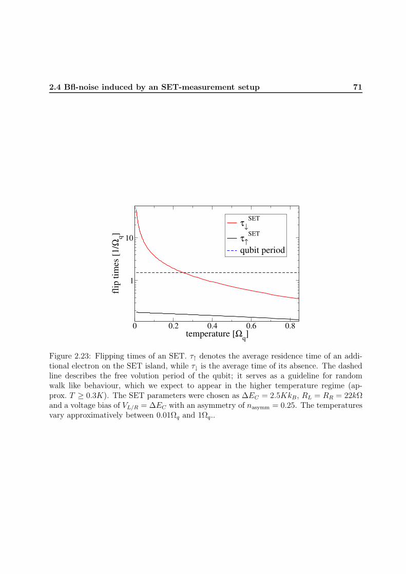
2.4 Bfl-noise induced by an SET-measurement setup 71
0 0.2 0.4 0.6 0.8temperature [Ωq]
1
10
flip
tim
es [1
/Ωq]
τ↓SET
τ↑SET
qubit period
Figure 2.23: Flipping times of an SET. τ↑ denotes the average residence time of an addi-tional electron on the SET island, while τ↓ is the average time of its absence. The dashedline describes the free volution period of the qubit; it serves as a guideline for randomwalk like behaviour, which we expect to appear in the higher temperature regime (ap-prox. T ≥ 0.3K). The SET parameters were chosen as ∆EC = 2.5KkB, RL = RR = 22kΩand a voltage bias of VL/R = ∆EC with an asymmetry of nasymm = 0.25. The temperaturesvary approximatively between 0.01Ωq and 1Ωq..

72 2. Qubit decoherence due to bistable fluctuators
0.01 0.1 1temperature [Ωq]
10
102
103
104
deca
y tim
es [1
/Ωq]
relaxation timesanalytical datadephasing timesanalytical data
Figure 2.24: Temperature dependence plot of the relaxation, respectively dephasing timesof a qubit exposed to SET induced bfl-noise. Numerically fitted values are compared withcorresponding analytical random walk results. Evidently the analytical prognosticatedbehaviour of τrel/deph ' µT−x is satisfied in good accuracy by the numerical data. Thephysical parameters of the qubit were given by εq = 1KkB and ∆q = 0.5KkB. The SETparameters were ∆EC = 2.5KkB, RL = RR = 22kΩ, VL/R = ∆EC and an asymmetry ofnasymm. The temperatures vary approximatively between 0.01Ωq and 1Ωq.
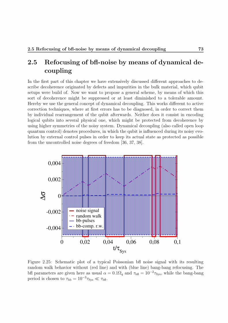
2.5 Refocusing of bfl-noise by means of dynamical decoupling 73
2.5 Refocusing of bfl-noise by means of dynamical de-
coupling
In the first part of this chapter we have extensively discussed different approaches to de-scribe decoherence originated by defects and impurities in the bulk material, which qubitsetups were build of. Now we want to propose a general scheme, by means of which thissort of decoherence might be suppressed or at least diminished to a tolerable amount.Hereby we use the general concept of dynamical decoupling. This works different to activecorrection techniques, where at first errors has to be diagnosed, in order to correct themby individual rearrangement of the qubit afterwards. Neither does it consist in encodinglogical qubits into several physical one, which might be protected from decoherence byusing higher symmetries of the noisy system. Dynamical decoupling (also called open loopquantum control) denotes procedures, in which the qubit is influenced during its noisy evo-lution by external control pulses in order to keep its actual state as protected as possiblefrom the uncontrolled noise degrees of freedom [36, 37, 38].
0 0,02 0,04 0,06 0,08 0,1t/τSys
-0,004
-0,002
0
0,002
0,004
∆σ
noise signalrandom walkbb-pulsesbb-comp. r.w.
Figure 2.25: Schematic plot of a typical Poissonian bfl noise signal with its resultingrandom walk behavior without (red line) and with (blue line) bang-bang refocusing. Thebfl parameters are given here as usual α = 0.1Ωq and τbfl = 10−2τSys, while the bang-bangperiod is chosen to τbb = 10−3τSys τbfl.

74 2. Qubit decoherence due to bistable fluctuators
2.5.1 Refocusing (bang-bang) scheme
The refocusing pulse sequence we suggest, also called bang-bang due to its rapidly anditeratively applied pulse sequences, is based on the same concept as the well-known Carr-Purcell-Gill-Meiboom echo technique first used in NMR [67] (an extension of the morefamiliar spin-echo method). The technique consist of averaging out of quasi-static devi-ations from the free Hamiltonian, generated by comparabely slow fluctuations of the bfl.As indicated in Fig. 2.25 rapidly flips of the qubit σqz-spin refocus the main fraction of thepure bfl-deviations,i.e. every integer numbers of bang-bang periods represents a spin-echocircle, as long as no bfl flip takes place. Only for unperturbed bang-bang periods (withoutbfl flips), this average scheme works perfectly. If a bfl flip occurs during one bang-bangcycle, there would arise remaining decoherence effects. Those spin-flips could be executede.g. by using infinitesimally short π-pulses in σqx-direction, applied on well-defined equallyseparated times (with iteration period τbb τbfl).
0,017 0,019 0,021 0,023t/τSys
-0.0002
-0.0001
0
0.0001
0.0002
∆σ
bang-bang pulsesbb-comp. random walkbfl noise signal
Figure 2.26: Detailed plot of the bang-bang refocused random walk (blue dot-dashed line)in dependence of the bfl flip positions (red line). As zoom extract from Fig.2.25 the samephysical parameters were given, i.e. α = 0.1Ωq, τbfl = 10−2τSys and τbb = 10−3τSys.

2.5 Refocusing of bfl-noise by means of dynamical decoupling 75
These spin-flips would lead to correspondingly fast sign-flipping of the noise term inthe Hamiltonian 2.5, thus to an averaging out of its decohering effect with respect to2.24, as each two bang-bang periods would refocus the Hq,bfl-induced deviations. Virtuallythe bang-bang pulses would reduce the bfl mean influence time τbfl during each inter-flipduration to a reduced time separation of τbb. Heuristically one would expect a decrease ofthe decoherence impact in the order of τbb/τbfl. As the frequency of the reduced randomwalk steps stays constant, we would expect as rule of thumb of the bang-bang refocusedrandom walk deviations
∆σbb(N) ∼ ατbb
√N . (2.72)
For technical convenience, we will assume the π-pulses to be of infinitesimal dura-tion. This is no crucial simplification, as detailed analysis of finite-length pulses below willconfirm. As one easily recognize, the bang-bang pulses will not only suppress the noisyσqz-term of the total Hamiltonian 2.23, but also any static σqz-part of the qubit Hamiltonian2.22. Theoretically this would reduce our feasible coherent qubit operations on only oneremaining degree of freedom, which is the same as the bang-bang pulses, as thereby com-mutation of pulses and static terms would permit them. But this restriction on feasiblequbit dynamicss can be circumvented, if one implements appropriate pulse sequences in σqxand σqy-direction. When chosing the σqz-refocusing driving simultaneously to the intendeddynamics, corresponding gate pulses are admitted [38].
2.5.2 Random walk model
In analogy to our random walk analysis of the pure bfl noise, we develop a detailed modelof the bang-bang refocused random walk. From there we obtain an accurate analyticalexpression for the remaining decoherence in its intermediate time regime. To evaluate aqualitative picture of the one-step deviations during bang-bang compensation, one has toconsider, that the bfl flip produces maximum abberration, if the symmetry of a bang-bangdouble-period is maximally broken. This is the case if the bfl flip coincides with the secondbang-bang pulse (in the middle of one double-period). As one can see from Fig.2.27 theusual pure σqx-evolution would then receive in the second part of the bang-bang period nota refocusing driving, but a deviation in the same direction. Thus, we obtain for this amaximal one-step deviation of 2ατbb. However, this abberation is scaled down by a factorof 1/
√2, as its impact is depending on the longitudinal angle χ of the spin present Bloch
sphere position, by a factor of sinχ. This is as the σqz-component of the noisy evolution doesnot influence the qubit if it is near the σqz = ±1-states, and its effect in- and decreases inbetween correspondingly. As we are mainly interested in mean aberrations for the regimeof several random walk steps, we simply average the maximal one-step deviation in typicalrms manner to
⟨∆σbb
max
⟩=
√1
2π
∫ 2π
0
sin2 χ4α2τ 2bb dχ =
√2ατbb. (2.73)

76 2. Qubit decoherence due to bistable fluctuators
Evidently this variance only contributes to relaxation, dephasing is strongly suppressed(see also Fig.2.28).
Figure 2.27: Sketch of a maximal one-step deviation during a bang-bang modulatedcycle, which appears if the bfl state flips precisely at the intermediate bang-bang pulsetime. The dephasing part of deviation evidently averages out, while a relaxating aberrancearise proportional to the noise-coupling constant α, as well as to sinχ with χ the actuallongitudinal angle of the spin position (measured from σqz = +1).
With this maximum one-bfl-flip deviation we can now formulate a corresponding one-step random walk distribution. Thereby we have to mention, that in contrast to our formerPoissonian distribution 2.29, the size of the random walk step is given by the actual positionof the bfl flip in the bang-bang double-period. The maximum effect is obtained, if the flip isexactly in the middle of such a double-period (i.e. when the second bang-bang pulse apply)and correspondingly linearly rescaled otherwise (until zero impact, if the flip is directly atthe begin or end of such a double-period). As we consider τbb τbfl, the position of bfl flips

2.5 Refocusing of bfl-noise by means of dynamical decoupling 77
in concerned double-periods appears total randomly, i.e. equally distributed, we receive forthe one-step random walk distribution of the bang-bang refocused system
Φbbodd/even(x) =
θ(±x)θ (γbb ∓ x)
γbb. (2.74)
with θ(x) the Heaviside-function. γ−bb =√
2ατbb corresponds to the maximum abberra-tion regarding 2.73. The difference between odd and even case is analogous to the up anddown states of the former pure bfl situation. It represents left and right deviation from theeffective trajectory of a noiseless evolution with bang-bang pulses.
0.01 1 100t / τSys
10-6
10-4
10-2
100
| ∆ σ
|
numericalanalyticalbang-bang numericalbang-bang analytical
0.01 1 1e+02
10-8
10-4
100
relaxationdephasing
Figure 2.28: Time evolution of the rms deviations for bfl-induced random walks withand without bang-bang control. The coupling constant is given as α = 0.1 and the meanflipping time scale is τbfl = 10−2τSys. The separation between two bang-bang pulses amountτbb = 10−3τSys. The straight lines are square-root fits of the analytical derived randomwalk model variances (plotted as triangles). Inset: Components of the deviations fromthe free precession trajectory that are parallel to it (dephasing) and perpendicular to it(relaxation/excitation) with bang-bang control.

78 2. Qubit decoherence due to bistable fluctuators
Analogous to the former situation, we can also express the 2Nbfl random walk distri-bution by means of the convolution theorem
Φbb2Nbfl
(x) = F−1[(
F[Φbb
2
])Nbfl]
=
∫ π
−π
dk
2πγ2Nbfle−ikx
([1− cos((γ + 1)k)]
[1− cos(k)]
)Nbfl
(2.75)
with F and F−1 denoting the discrete Fourier transformation and its inverse, respectively.
Applying the saddle point approximation again we obtain for the Gaussian mean devi-ation
∆σbb(Nbfl) =√Nbfl
γbb
2=√Nbfl
1√2ατbb . (2.76)
Which appearantly fits very accurately with the corresponding numerical simulations (seeFig.2.28).
0
0.2
0.4
0.6
0.8
1
–1 –0.5 0.5 1 0
0.2
0.4
0.6
0.8
1
–1 –0.5 0.5 1
Figure 2.29: Comparison of two-step distributions for the random walks with bang-bangcontrol with pulse shapes that are taken to be δ-functions (left) versus a continuous sinewave sin( π
τbbt) (right). For clarity, the y-axis is rescaled to the maximum values of the
distributions, while the x-axis is given in units of γbb.
2.5.3 Pulse shapes
At first sight, treating bang-bang pulses as δ-function impulses appears to be an extraor-dinarily strong assumption. This in particular as in a practical implementations, the large
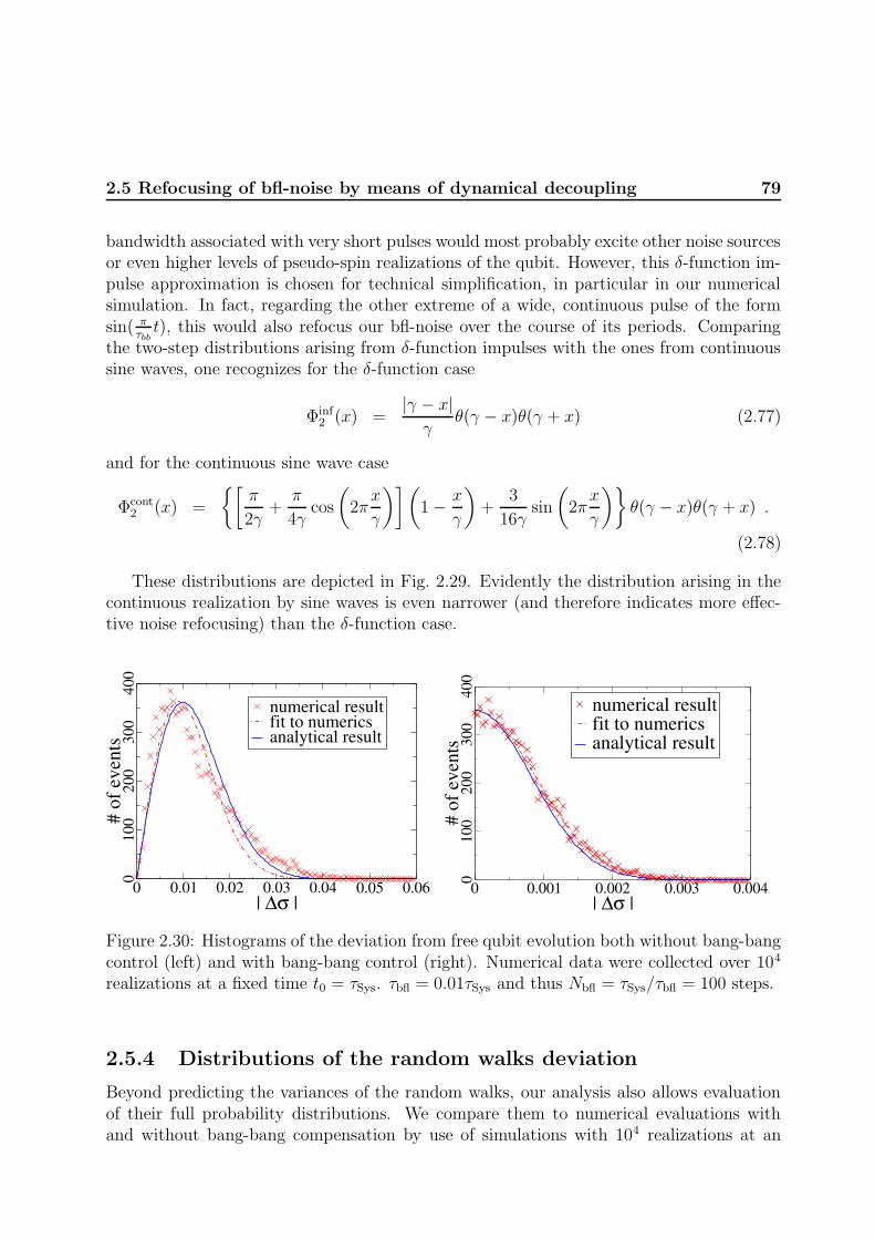
2.5 Refocusing of bfl-noise by means of dynamical decoupling 79
bandwidth associated with very short pulses would most probably excite other noise sourcesor even higher levels of pseudo-spin realizations of the qubit. However, this δ-function im-pulse approximation is chosen for technical simplification, in particular in our numericalsimulation. In fact, regarding the other extreme of a wide, continuous pulse of the formsin( π
τbbt), this would also refocus our bfl-noise over the course of its periods. Comparing
the two-step distributions arising from δ-function impulses with the ones from continuoussine waves, one recognizes for the δ-function case
Φinf2 (x) =
|γ − x|γ
θ(γ − x)θ(γ + x) (2.77)
and for the continuous sine wave case
Φcont2 (x) =
[π
2γ+
π
4γcos
(2πx
γ
)](1− x
γ
)+
3
16γsin
(2πx
γ
)θ(γ − x)θ(γ + x) .
(2.78)
These distributions are depicted in Fig. 2.29. Evidently the distribution arising in thecontinuous realization by sine waves is even narrower (and therefore indicates more effec-tive noise refocusing) than the δ-function case.
0 0.01 0.02 0.03 0.04 0.05 0.06| ∆σ |
010
020
030
040
0#
of e
vent
s
numerical resultfit to numericsanalytical result
0 0.001 0.002 0.003 0.004| ∆σ |
010
020
030
040
0#
of e
vent
s
numerical resultfit to numericsanalytical result
Figure 2.30: Histograms of the deviation from free qubit evolution both without bang-bangcontrol (left) and with bang-bang control (right). Numerical data were collected over 104
realizations at a fixed time t0 = τSys. τbfl = 0.01τSys and thus Nbfl = τSys/τbfl = 100 steps.
2.5.4 Distributions of the random walks deviation
Beyond predicting the variances of the random walks, our analysis also allows evaluationof their full probability distributions. We compare them to numerical evaluations withand without bang-bang compensation by use of simulations with 104 realizations at an

80 2. Qubit decoherence due to bistable fluctuators
evolution time t0 = τSys. The numerical histograms of the deviations with their respectiveone- and two-dimensional Gaussian fits are shown in Fig. 2.30.
We observe that not only the distribution obtained with bang-bang control is muchnarrower than the distribution for pure bfl noise, but also that its shape is qualitativelydifferent. The maximum of the bang-bang controlled distribution is at zero error. Incontrast, the uncontrolled distribution has its maximum at a finite error |∆σ|max ≈ 0.01,and it has zero probability of zero error. This reflects the one-dimensional nature of thebang-bang controlled random walk on the Bloch sphere in contrast to the generic two-dimensional expansion of the pure bfl random walk.
2.5.5 Bang-bang control working as a high-pass filter
In order to measure the degree of noise suppression due to bang-bang control, we define asuppression ratio St0 as follows for a given evolution time t0
St0(τbfl/τbb) ≡ ∆~σbflrms(t0)
∆~σbbrms(t0)
. (2.79)
101 102 103 104105
τ bfl / τ bb
100
101
102
103
104
105
106
S t 0 (
τ bfl
/ τ b
b )
Numerical resultlinear fit
Figure 2.31: The suppression factor St0(τbfl/τbb) = ∆~σbflrms(t0)
∆~σbbrms(t0)
evaluated for t0 = τSys as a
function of the ratio τbfl/τbb of the mean fluctuator time and the bang-bang pulse separation.

2.5 Refocusing of bfl-noise by means of dynamical decoupling 81
We now systematically study the dependence of St0 on τbfl/τbb for a constant mean bflswitching rate τbfl = 10−2τsys at a fixed evolution time t0 = τsys. The numerical data inFig. 2.31 show that the suppression efficiency is linear in the bang-bang repetition rate,Sτsys = µτbfl/τbb. The numerically derived value of the coefficient, µnumerical ≈ 1.679, shows
good agreement with our analytical result µanalytical =√
5/2 ' 1.581 from the saddle pointapproximation, eq. (2.31) and (2.76).
This small discrepancy between the numerical and analytical results is due to the factthat our analytical calculations neglect correlations between the parallel (dephasing) andperpendicular (relaxating/exciting) components of the random walk. This leads to anunderestimate of the rms-deviation ∆~σbfl
rms in the case without bang-bang control (comparealso to Fig. 2.30). Therefore, we have quantitatively proven our qualitative intuition: bang-bang control affects the bfl noise signal working like a high-pass filter, an effect which wasgenerally predicted for dynamical decoupling techniques [37].

82 2. Qubit decoherence due to bistable fluctuators
2.5.6 Bang-bang refocusing of finite temperature bfl-noise
After having examined the high-pass filter behaviour of the refocusing of an idealized, sym-metric bistable fluctuator we want to expand our investigations of bang-bang efficiency onthe mere realistic case of temperature dependent bfl-noise. Thereby we apply our formermodel of temperature dependence, expressed concisely in eq. (2.37).
0 2 4 6 8 10Temperatur [Ωq]
0,0
2,5×10
-45,0
×10-4
7,5×10
-41,0
×10-3
∆σ
num. data at Ωq t = 1400num. data at Ωq t = 140num. data at Ωq t = 14bb-model: Ωq t = 1400bb-model: Ωq t = 140bb-model: Ωq t = 14
0 2 4 6 8 10Temperatur [Ωq]
0
2×10⁻³
4×10⁻³∆σ
num. data at Ωq t = 1400num. data at Ωq t = 140num. data at Ωq t = 14bb-model: Ωq t = 1400bb-model: Ωq t = 140bb-model: Ωq t = 14
0 2 4 6 8 10Temperatur [Ωq]
0,0
5,0×10
-31,0
×10-2
1,5×10
-22,0
×10-2
∆σ
num. data at Ωq t = 1400num. data at Ωq t = 140num. data at Ωq t = 14bb-model: Ωq t = 1400bb-model: Ωq t = 140bb-model: Ωq t = 14
0 2 4 6 8 10Temperatur [Ωq]
0,0
2,5×10
-25,0
×10-2
7,5×10
-21,0
×10-1
∆σ
num. data at Ωq t = 1400num. data at Ωq t = 140num. data at Ωq t = 14bb-model: Ωq t = 1400bb-model: Ωq t = 140bb-model: Ωq t = 14
Figure 2.32: Temperature dependences of dynamically refocused bfl-noise deviations atdifferent bang-bang time scales τbb = 10−13s ' 7 · 10−4/Ωq (plot left top), τbb = 5 · 10−13s' 3.5 · 10−3/Ωq (right top), τbb = 2 · 10−12s ' 1.4 · 10−2/Ωq (left bottom) and τbb = 10−11s' 7 · 10−2/Ωq (right bottom). The coupling constant between qubit and bfl is chosen asα = 0.01Ωq, the bfl-Bath coupling parameter accounts λ = 102. Its bfl flipping rates aregiven by eq. 2.37 with parameters ∆bfl = 1/
√1.01 · 109 Hz and εbfl = 1/
√1.01 · 1010 Hz.
Under the assumption, that the bang-bang pulse sequence period is much faster than the

2.5 Refocusing of bfl-noise by means of dynamical decoupling 83
typical bfl flipping times we expect an analogous one-step deviation of the correspondingrefocused random walk as described in the symmetric bfl-noise case (eq. (2.73)). Applyingthe corresponding temperature dependent time distribution of (double) steps we receivean effective refocused random walk deviation of
∆σasymmbb (t) =
√t
τmeanbfl
√2ατbb =
√2t
(τ ↑bfl + τ ↓bfl)
√2ατbb
=
√4t
2(e−Ωbflβ/2 + eΩbflβ/2) sinh(Ωbflβ/2) Ωbfl
λ∆2bfl
ατbb (2.80)
=
√tλ∆2
bfl
cosh(Ωbflβ/2) sinh(Ωbflβ/2)Ωbfl
ατbb =
√2t
sinh(Ωbflβ)
√λ∆2
bfl
Ωbfl
ατbb.
One clearly recognizes in Fig. 2.32 the approximative√T -like behaviour (for small tem-
peratures, i.e. Ωbflβ < 1), which agrees perfectly with the analytically predicted standarddeviations. Only small disagreements between analytical and numerical datas were visiblein the case of low-frequently bang-bang pulses (τbb = 10−11 s).
0 2 4 6 8 10Temperatur [Ωq]
0
1×10⁻³
2×10⁻³
3×10⁻³
∆σ (τ
bb =
10-1
3 s ≈
7 1
0-4Ω
q )
num. data at Ωq t = 1400num. data at Ωq t = 140num. data at Ωq t = 14bb-model: Ωq t = 1400bb-model: Ωq t = 140bb-model: Ωq t = 14
0 2 4 6 8 10Temperatur [Ωq]
0,0
5,0×10
-3
1,0×10
-2
1,5×10
-2
∆σ (
τ bb =
5 1
0-13 s
≈ 3
.5 1
0-3Ω
q )
num. data at Ωq t = 1400num. data at Ωq t = 140num. data at Ωq t = 14bb-model: Ωq t = 1400bb-model: Ωq t = 140bb-model: Ωq t = 14
0 2 4 6 8 10Temperatur [Ωq]
0
1×10⁻²
2×10⁻²
3×10⁻²
∆σ (τ
bb =
10-1
2 s ≈
7 1
0-3Ω
q)
num. data at Ωq t = 1400num. data at Ωq t = 140num. data at Ωq t = 14bb-model: Ωq t = 1400bb-model: Ωq t = 140bb-model: Ωq t = 14
0 2 4 6 8 10Temperatur [Ωq]
0
2×10⁻²
4×10⁻²
6×10⁻²
8×10⁻²
∆σ (τ
bb =
2 1
0-12 s
≈ 1
.4 1
0-2Ω
q)
num. data at Ωq t = 1400
num. data at Ωq t = 140
num. data at Ωq t = 14
bb-model: Ωq t = 1400
bb-model: Ωq t = 140
bb-model: Ωq t = 14
bfl-model: Ωq t = 1400
bfl-model: Ωq t = 140
bfl-model: Ωq t = 14
0 2 4 6 8 10Temperatur [Ωq]
0,0
3,0×10
-26,0
×10-2
9,0×10
-21,2
×10-1
∆σ (τ
bb =
10-1
3 s ≈
7 1
0-4Ω
q)
num. data at Ωq t = 1400
num. data at Ωq t = 140
num. data at Ωq t = 14
bb-model: Ωq t = 1400
bb-model: Ωq t = 140
bb-model: Ωq t = 14
bfl-model: Ωq t = 1400
bfl-model: Ωq t = 140
bfl-model: Ωq t = 14
0 2 4 6 8 10Temperatur [Ωq]
0,0
3,0×10
-26,0
×10-2
9,0×10
-21,2
×10-1
∆σ (τ
bb =
10-1
1 s ≈
7 1
0-2Ω
q)
num. data at Ωq t = 1400
num. data at Ωq t = 140
num. data at Ωq t = 14
bb-model: Ωq t = 1400
bb-model: Ωq t = 140
bb-model: Ωq t = 14
bfl-model: Ωq t = 1400
bfl-model: Ωq t = 140
bfl-model: Ωq t = 14
Figure 2.33: Temperature dependence of dynamical refocused bfl-noise deviations at var-ious bang-bang time scales (see corresponding specifications at the y-axis). The τbfl-ratesare given by eq. (2.37) with bfl parameters ∆bfl = 109/
√1.01 Hz, εbfl = 1010/
√1.01 Hz and
λ = 102. The qubit-bfl coupling accounts α = 0.01Ωq.

84 2. Qubit decoherence due to bistable fluctuators
In contrast to plot 2.32 the agreement between numerical data and refocused randomwalk analysis is much worse for to faster bfl flipping times (see Fig. 2.33); for longer bang-bang periods and higher temperatures it almost reaches the form of the uncompensatedbfl random walk. This is not surprising, as with increasing bang-bang periods for decreas-ing bfl flipping times the basic assumption of constant single-step distributions (eq. 2.29)crosses over to the original bfl random walk distributions (eq. C.9). As consequence wereceive qualitatively pure bfl noise like behaviour, with slightly reduced amplitude due tothe remaining refocusing effects.
If we now plot the suppression factor St0(τbb) (2.79) for given qubit and bfl parameters(∆q = εq = 1010 Hz, ∆bfl = 0.1εbfl = 109√
1.01Hz, α = 0.01) at low and high frequently
bfl-noise (i.e. λ = 100, respectively λ = 1000) we observe the following behaviour.
0.001 0.01 0.1τbb [1/Ωq]
101
102
103
S t 0(T)
St0 at T=0.1 Ωq
St0 at T=0.14 Ωq
St0 at T=0.2 Ωq
St0 at T=0.3 Ωq
St0 at T=0.5 Ωq
St0 at T=0.7 Ωq
St0 at T=1 Ωq
St0 at T=1.4 Ωq
St0 at T=2 Ωq
St0 at T=3 Ωq
St0 at T=5 Ωq
St0 at T=7 Ωq
St0 at T=10 Ωq 0.001 0.01 0.1
τbb [1/Ωq]100
101
102
S t 0(T)
St0 at T=0.1 Ωq
St0 at T=0.14 Ωq
St0 at T=0.2 Ωq
St0 at T=0.3 Ωq
St0 at T=0.5 Ωq
St0 at T=0.7 Ωq
St0 at T=1 Ωq
St0 at T=1.4 Ωq
St0 at T=2 Ωq
St0 at T=3 Ωq
St0 at T=5 Ωq
St0 at T=7 Ωq
St0 at T=10 Ωq
Figure 2.34: Suppression factors of bang-bang refocusing, applied on bfl-noise of varioustemperatures (between Tmin = 0.0014Ωq and Tmax = 0.14Ωq), evaluated at time t0 = 10−7
s. Besides usual qubit and bfl properties (∆q = εq = 1010 Hz, ∆bfl = 109√1.01
Hz, εbfl = 1010√1.01
Hz and α = 0.01 ·1010 Hz), we consider compareably low and high frequency bfl-noise givenby λ = 100 (left plot), respectively λ = 1000 (right plot).
Obviously for the low-frequent bfl case we receive in good accuracy the expected lineardependence of the suppression factor on the time scale ratio τbfl/τbb (i.e. antilinear in τbb).In the high-frequent bfl situation we recognize for higher temperatures and lower τbb, thatcomparable bfl and bang-bang time scales lead to vanishing compensation efficiency and to
a saturation effect of St0(τbfl/τbb)τbfl/τbb→1−→ 1. If one consider the temperature dependence
of the suppression ratio for given bang-bang periods (Fig. 2.35), one can see similarily howthe bfl-noise compensation saturates for higher temperatures and lower bang-bang pulsefrequencies converging to almost no positive effect.

2.5 Refocusing of bfl-noise by means of dynamical decoupling 85
0.1 1 10Temperature [Ωq]
100
101
102
103
S t 0
St0 at Ωqτbb = 0.014
St0 at Ωqτbb = 0.028
St0 at Ωqτbb = 0.07
St0 at Ωqτbb = 0.14
St0 at Ωqτbb = 0.28
St0 at Ωqτbb = 0.7
St0 at Ωqτbb = 1.4
0.1 1 10Temperature [Ωq]
100
101
102
S t 0
St0 at Ωqτbb = 0.014
St0 at Ωqτbb = 0.028
St0 at Ωqτbb = 0.07
St0 at Ωqτbb = 0.14
St0 at Ωqτbb = 0.28
St0 at Ωqτbb = 0.7
St0 at Ωqτbb = 1.4
Figure 2.35: Suppression factors of various bang-bang pulse periods (τbb from 10−13s to10−11s), applied on bfl-noise as function of temperatures (between Tmin = 0.01 K andTmax = 1 K), evaluated at time t0 = 10−7 s. Given usual qubit and bfl properties (∆q =
εq = 1010 Hz, ∆bfl = 109√1.01
Hz, εbfl = 1010√1.01
Hz and α = 0.01 · 1010 Hz), we considered
compareably low (left) and high (right) frequent bfl-noise (corresponding to λ = 100,respectively λ = 1000).
2.5.7 Applicability of imperfect bang-bang pulses
Thus far, we have tacitly assumed that one is capable to produce perfect, zero-width π-pulses exactly along the σx-axis of the Bloch sphere. We now take into account, that thecontrol pulses themselves can have slight fluctuations in regard of their duration or direc-tion. This would interfere with the desired refocusing. As already shown at the end ofsection2.5.2, the restriction of pulses to infinitesimal duration can be significantly relaxed.Now we investigate to what extent the restriction to perfectly applied pulses can be relaxed.
We essentially analyze two generic types of errors that could occur in the control ap-paratus when trying to apply π-pulses in σx-direction. At first, the duration of each pulsecould exhibit fluctuations, preoducing fluctuations in the resulting rotation-angle aroundthe desired value of π. Secondly, the polarization axis could suffer from directional devi-ations around the desired direction (i.e. of σx). Assuming the statistical independence ofeach pulse error, we expect for both types of imperfections a random-walk-like behaviourof cumulating deviations compared to evolutions with perfect pulses.
One-dimensional pulse error (dephasing)
We make the quite general assumption that we may model the one-dimensional phase fluc-tuation of the imperfect bang-bang pulses φj(x) as a Gaussian distribution of the pulsedurations and therefore of the rotation angles around their intended value π. This isno crucial restriction, as we expect that any roughly symmetric and smooth distributionof fluctuations will produce Gaussian formed total distributions after several inaccuratebang-bang steps, satisfying the central limit theorem. The Gaussian distribution is param-eterized by its standard deviation δφ0 (see Fig. 2.36). Thus, the corresponding pulse angle

86 2. Qubit decoherence due to bistable fluctuators
aberration of the jth step is given by
φ1dj (x) =
1√2πδφ0
e− x2
2δφ02 . (2.81)
Having assumed a Gaussian distribution, we can exactly evaluate the distributions of theN -step deviation ∆ΦN (which are usually given as N -fold time-convoluted integrals) byuse of the convolution theorem as follows
Φ1dN = F−1
[ΠNj=1φj
]
=1√
2πNδφ0
e− x2
2Nδφ02 (2.82)
with φ1dj = F [φj] denoting the Fourier transformed of φ1d
j and F−1 the inverse Fouriertransformation.
Figure 2.36: Sketch of one-dimensional bang-bang aberration. The variations δφ0 of therotation angle around the desired value of π leads to slight deviations in parallel to thepermitted dynamical direction, thus generating dephasing.

2.5 Refocusing of bfl-noise by means of dynamical decoupling 87
Consequently the rms displacement in the random walk increases as square-root of thenumber N of bang-bang pulses: δφN =
√Nδφ0. Equivalently, the dephasing grows as
square-root in time
δφ(t) =√t/τbbδφ0 (2.83)
on the time scale of our coarse-graining (which is here given as τbb).
Two-dimensional pulse error (dephasing as well as relaxation/excitation)
A similar argument works when there appear fluctuations around the desired σx rotationaxis. Each individual variation of the axis can be split into two components: (1) δφperp,which is perpendicular to the connecting vector between the σx-axis and the qubit state~σ(t) on the Bloch sphere, and (2) δφtan, which is transverse to it (see Fig. 2.37). Tofirst order, the perpendicular part does not disturb the intended spin-flip 2. However, thetransverse part does cause a deviation from the ideal spin-flip in a direction toward oraway from the previous qubit state. Therefore, it produces relaxation or excitation, asits effect is orthogonal to the free σx-evolution. In a statistical average we only have toconsider a fraction of 1/
√2 of the typical total mean δφ0 of the aberration. The effect of
a π-rotation around an axis tilted by an angle δφtan is a deviation 2δφtan from the trajec-tory of the perfect evolutions; thus we receive altogether a deviation on the order of
√2δφ0.
From there we obtain analogously to Equ. (2.81) for each single step distribution
φ2dj (x) =
1√2π√
2δφ0
e− x2
4δφ02 ; (2.84)
and analogously to Equ. 2.82 for the deviation after N steps
Φ2dN =
1√2π√
2Nδφ0
e− x2
4Nδφ02 . (2.85)
Equivalently, in terms of the time t
δφ(t) =√
2t/τbb · δφ0 . (2.86)
2.5.8 Numerical and analytical results
In the same manner as our previous integrations of a stochastic Schrodinger equation, wenumerically simulate qubit dynamics under inaccurate pulses. In the first instance, wework without bfl-noise to verify our analytical random walk model. Later, we add thebfl-noise in order to study the competition between the two sources of error.
2The attentive reader might object here, that a spin-flip around a different axis on the xy-equatordoes not commute with pure σx-dynamics, but rather with something nearby. As we do not consider anyσy-components yet, we do not bother about the minimal distortion of pure σx-operations, which can beestimated to be on the 2nd order of the aberration parameter δφ0, which we assume to be very smallanyway.

88 2. Qubit decoherence due to bistable fluctuators
Figure 2.37: Sketch of two-dimensional bang-bang aberration. To first order, variationsδφperp of the rotation axis perpendicular to the connection vector between σx and the qubitstate (here for simplicity: σz = +1) do not influence the intended spin-flip, whereas thevariations δφtan along this line causes deviations on the Bloch sphere perpendicular to thepermitted evolution trajectories (therefore producing relaxation or excitation).
Random walk due to inaccurate bang-bang pulses only
We analyze deviations on the Bloch sphere between the noiseless case trajectories thatoccur when the bang-bang pulses are perfect and those when they are not. As describedin eq. (2.33), we calculate the rms-deviation over ensembles of N = 103 realizations. Asa representative time point we take t0 = τSys. This is an appropriate choice, as explainedin the discussion of Fig. 2.13, this time scale should exhibit neither short-time effects nornear-total decoherence. From eq. (2.83) and (2.86) it immediately follows, that for themean deviations at t0 results if there are phase errors
∆σ1dbb(t0) =
√Nbbδφ0 =
√t0τbb
δφ0 , (2.87)

2.5 Refocusing of bfl-noise by means of dynamical decoupling 89
and if there are axis errors
∆σ2dbb(t0) =
√2Nbbδφ0 =
√2t0τbb
δφ0 . (2.88)
100 10000 1e+06# of bang-bang pulses
1e-0
60.
0001
0.01
1r.w
. mea
n de
viat
ion
numerical data for δφ = 10-4
numerical data for δφ = 10-5
numerical data for δφ = 10-6
analytical curves
100 10000 1e+06# of bang-bang pulses
0.00
010.
011
r.w. m
ean
devi
atio
n
numerical data for δφ = 10-4
numerical data for δφ = 10-5
numerical data for δφ = 10-6
analytical curves
Figure 2.38: Plot of the one- respectively two-dimensional imperfectly bang-bang pulsedevolution. Dashed lines are square-root fits of the numerical data, while the solid linesdenotes the analytical calculations.
As characteristic values for the mean accuracy of single pulses, we choose δφ0 in therange of 10−6 to 10−4, which should be technologically feasible. As one can see in thedouble logarithmic plots of Fig. 2.38, the numerically determined evolutions follow theanalytically expected square-root type random walk behavior.
Random walk due to inaccurate bb-pulses and bfl-noise
We now combine our imperfect bang-bang pulse operations with our former bfl-noise signalto discuss the applicability of our control scheme when realistic pulse generators are used.As before, we calculate the rms deviations at t0 = τSys by averaging over 103 realizations.The bfl-parameters are the same used previously: a coupling strength α = 0.1 and anaverage switching time τbfl = 0.01τSys. However, with the aim of determining the optimalbang-bang protocol in the presence of pulse imperfections, we now consider different pulseseparation times τbb/τSys ranging from 10−5 to 10−2.

90 2. Qubit decoherence due to bistable fluctuators
1e-05 0.0001 0.001 0.01τbb / τbfl
0.00
010.
001
0.01
0.1
r.w. m
ean
devi
atio
n
numerical data for δφ = 10-4
numerical data for δφ = 10-5
numerical data for δφ = 10-6
analytical curves
1e-05 0.0001 0.001 0.01τbb / τbfl
0.00
010.
001
0.01
r.w. m
ean
devi
atio
n
numerical data for δφ = 10-4
numerical data for δφ = 10-5
numerical data for δφ = 10-6
analytical curves
Figure 2.39: Plot of the Bloch sphere rms deviations received by one-/two-dimensionalinaccurately pulsed bang-bang compensation of the typical bfl-perturbation. Dashed linesdescribe the aberrances for pure faulty bang-bang (i.e. without bfl-noise), respectivelythe exactly compensated bfl-case (see Fig. 2.13), while solid lines denotes the deviationscalculated by random walk analysis.
We assume that the errors induced by the bfl and those induced by the pulse generatorare statistically independent, and thus we can add them in the usual rms-fashion. Incomparison to the case of ideal bang-bang pulses, eq. (2.76), we find here the average totaldeviations induced by both bfl telegraph noise and imperfect bang-bang pulses to be
∆σ1dtot =
√∆σ2
bfl + ∆σ1dbb
2
=
√1
2Nbflα2τ 2
bb +Nbbδφ20 (2.89)
=
√1
2α2τ 2
bb
t0τbfl
+ δφ20
t0τbb
in the one-dimensional case where imperfect pulses only impart phase errors (due to im-precise pulse duration), and
∆σ2dtot =
√∆σ2
bfl + ∆σ2dbb
2
=
√1
2Nbflα2τ 2
bb + 2Nbbδφ20 (2.90)
=
√1
2α2τ 2
bb
t0τbfl
+ 2δφ20
t0τbb

2.5 Refocusing of bfl-noise by means of dynamical decoupling 91
in the two-dimensional case when imperfect pulses impart both phase and relaxation/excitationerrors (due to imprecision in the pulses’ polarization axis).
As Fig. 2.39 demonstrates, we observe a very good agreement between our numericaland analytical results. Such data make it possible to determine an optimal bang-bangseparation time τ opt
bb . Specifically, this optimum can be derived by calculating the zerovalue of the derivative of eq. (2.89) and (2.90) with respect to τbb. We therefore concludethat the optimal period between bang-bang pulses is
τ 1dbb =
3
√τbfl
δφ20
α2(2.91)
for the one-dimensional case and
τ 2dbb =
3
√2τbfl
δφ20
α2(2.92)
for the two-dimensional case. These optimal times respectively correspond to minimizedvariances at t0 = τSys of
∆σ1dopt =
√1
2+ 1
α1/3δφ2/30
τ1/6bfl
√t0 (2.93)
for the one-dimensional case of only imprecise pulse durations and
∆σ2dopt =
√2−1/3 + 22/3
α1/3δφ2/30
τ1/6bfl
√t0 (2.94)
for the two-dimensional case of both imprecise pulse durations and polarization axis.

92 2. Qubit decoherence due to bistable fluctuators

Chapter 3
Quantum phase diagram of a coupledqubit system
In this chapter we investigate the disappearance of coherence as well as entanglement of acoupled two spin system attached to two different sorts of bosonic Baths, which representslocalized and collective error sources. In contrast to our former decoherence analysis, we donot to focus on time evolutions, generated by appropriate master equations. We are ratherinterested in the occurrence, respectively suppression of coherence and entanglement of thetwo-spin system as a function of the dissipative coupling strengths to both kinds of baths.Thus we will mainly discuss static features of the dressed double spin system, technicallyafter having derived an effective pure spin Hamiltonian, that only implicitly depends onthe bath couplings. These dynamical and entanglement properties hereby were derived byconsidering the corresponding fixed point Hamiltonian, derived by means of an appropriatescaling analysis of the effective spin-operators couplings.
3.1 The 2-spins-3-bosonic-baths model
The theoretical model is constituted as follows; two spins with local coherent dynamicsgiven by ∆0σ
xj were coupled to each other by a σy1 ⊗ σy2 type interaction of the strength ∆I.
This quantum system itself is attached to one common Bosonic bath via a (σz1 + σz2)-term,as well as to two local baths, whose interaction is also of σzj -form. This pareticular choiceof coupling offers maximal mutual interactions of the coupling, as none of them commutewith the others.
The total 2-spin-3-baths Hamiltonian reads as follows
H2s3b = HS1 + HS2 + HS12 + HS1,Blocal+ HS2,Blocal
+ HS,Bcoll+ HB , (3.1)
with intra-spin dynamics on the jth spin
HSj=
∆0
aσxj (3.2)

94 3. Quantum phase diagram of a coupled qubit system
and spin-spin coupling of Ising type
HS12 =∆I
a(σy1 ⊗ σy2) . (3.3)
Figure 3.1: Schematic plot of a 2-spin-3-Bosonic-baths model. In order to receive a maximaldegree of mutual influences of the different interactions, non-commutativity for the single-spin, the double-spin, as well as the bath-spin couplings is chosen.
The normalization factor 1/a corresponds to the band-width of the Bosonic bath. Thecoupling to the dissipative baths is distinguished into the localized parts
HSj,Blocal=
1
2λlocalσ
zj
∂Φj
∂x(3.4)
and the collective one
HSBcoll=
1
2λcoll (σz1 + σz2)
∂Φ3
∂x, (3.5)
while dynamics of the bosonic baths are given in field theoretical notation [68] by
HB =∑
µ∈1,2,3
∫ L/2
−L/2
1
2∗∗ [∂xΦµ(x)]2 ∗∗
dx
2π+
2π
2LNµ
(Nµ + 1− δboundary
), (3.6)

3.1 The 2-spins-3-bosonic-baths model 95
which is equivalent to the harmonic oscillator bath representation used in chapter 1.
L denotes the (usually spatial) size of the Bosonic system(s), ∂xΦ ist abbreviated for∂Φ(x)∂x
, Nµ were the corresponding Bosonic excitation number operators. δboundary takesinto account boundary conditions (e.g. periodic or anti-periodic ones), for details [68] andreferences therein are recommended.
Note also, that this description of the origin of decoherence as bosonic baths doesnot necessarily disqualify fermionic noise sources (e.g. as one encounters with fluctuationof electronic leads), as in particular fermi sea environments can formally be interpretedbosonically by use of appropriate bosonization rules (see [68]).
A possible experimental realization of this setup would appear as suggested in Fig. 3.2.Here the σjx type dynamics on the spins would be driven by the embraced magnetic flux oftwo Josephson flux qubit. The spin-spin interaction σy1 ⊗ σy2 could be implemented by anelectro-magnetic coil, while the collective, as well as localized noise sources would be givenby the impedances of the common, respectively individual supply lines.
Figure 3.2: Schematic plot of the electric circuit realization of the 2-spin-3-Bosonic-bathsmodel by means of Josephson flux qubits. The σxj coupling on each spin is controlled bythe enclosed magnetic field, while the spin-spin interaction is given by an external coil.The localized, as well as common bath coupling is generated by the dissipative impedancesin the single, respectively common supply lines.

96 3. Quantum phase diagram of a coupled qubit system
3.2 The dressed double-spin Hamiltonian
In the following we want to apply an appropriate unitary transformation (the Emery-Kivelson transformation [69, 70]) on the 2-spins-3-Bosonic-baths Hamiltonian. This is inorder to receive an expression, which explicitly only depends on effective (so-called dressed)spin degrees of freedom. At first we therefor have to reorder some terms, for technical rea-sons as well as for making the symmetry effects of our transformation more visible.
For the spin-bath Hamiltonian we combine the collective and the localized terms to asymmetric and an antisymmetric part of spin-bath interaction
HSB = HS,Bcoll+ HS1,Blocal
+ HS2,Blocal
=1
2(σz1 + σz2)
(λcoll∂xΦ3 + 1/
√2λlocal∂xΦS
)+
+1
2(σz1 − σz2) 1/
√2λlocal∂xΦA
=1
2(σz1 + σz2)λS∂xΦS +
1
2(σz1 − σz2)λA∂xΦA , (3.7)
here we introduced for the sake of clarity as new coupling constants and Bosonic fields
λS =
√λ2
coll +λ2
local
2(3.8)
∂xΦS =1
λ
(λcoll∂xΦ3 + 1/
√2λlocal (∂xΦ1 + ∂xΦ2)
)(3.9)
for the symmetric case and
λA =λlocal√
2(3.10)
∂xΦA =1√2
(∂xΦ1 − ∂xΦ2) (3.11)
for the antisymmetric one.
For the single as well as double-spin interactions we replace the former Pauli-spin matrixterms σxj , σyj and σzj by corresponding combinations of σ±j operators defined by
σ±j =1
2
(σxj ± iσyj
), (3.12)
such that
HSj=
∆0
aσxj =
∆0
a
(σ+j + σ−j
), (3.13)

3.2 The dressed double-spin Hamiltonian 97
and
HS12 =∆I
a(σy1 σ
y2) =
∆I
a
[−(σ+
1 σ+2 + h.c.
)+(σ+
1 σ−2 + h.c.
)]. (3.14)
This is useful, as the latter transformation relations for the σ±j -terms are more easy to cal-culate. Anyway, as σ±j represents spin-up respectively spin-down flips, the mathematicalresults later on obtain easy to recognize physical interpretations.
As we furthermore will encounter different scaling behaviour for the σ±1 σ±2 terms as for
to the σ±1 σ∓2 ones, we will introduce here distinct coupling constants for both terms
HS12 =∆++
a
(σ+
1 σ+2 + h.c.
)+
∆+−a
(σ+
1 σ−2 + h.c.
). (3.15)
3.2.1 The Emery-Kivelson-transformation
The Emery-Kivelson-transformation [69, 70] for our two different bath terms (symmetricand antisymmetric)is given as
U(α, β) = exp
[i
(α
1
2(σz1 + σz2) ΦS + β
1
2(σz1 − σz2) ΦA
)]. (3.16)
If we apply this unitary transformation on our total Hamiltonian
Hdressed2s3b := U(α, β)H2s3bU
†(α, β) (3.17)
some algebra following the Bosonic commutation relation
[Φ, ∂xΦ] = i1l (3.18)
via the Baker-Hausdorff-formula (appendix C in [68])
exp (iγΦ) [∂xΦ]2 exp (−iγΦ) = [∂xΦ− γ1l]2 (3.19)
leads from HB to prefactor changes of the explicit bath-spin interactions of
HdressedB + Hdressed
SB =∑
µ∈1,2,3
∫ L/2
−L/2
1
2∗∗ [∂xΦµ(x)]2 ∗∗
dx
2π+
2π
2LNµ
(Nµ + 1− δboundary
)+
+1
2(σz1 + σz2) (λS − α) ∂xΦS +
1
2(σz1 − σz2) (λA − β) ∂xΦA +
+ constant terms , (3.20)

98 3. Quantum phase diagram of a coupled qubit system
such that the explicit spin-bath term HSB of the 2s3B-Hamiltonian disappears for thechoice
α = λS β = λA. (3.21)
Here we disregard any constant offsets, we receive from HdressedB and Hdressed
SB . A more de-tailed discussion can be found [71].
According the spin-operator commutation rules[σzj , σ
±k
]= ±δj,kσ∓k (3.22)
and Baker-Hausdorff
exp (iδ (σz1 + σz2)) σ±j exp (−iδ (σz1 + σz2)) = σ±j exp (∓iδ) , (3.23)
respectively
exp (iδ (σz1 − σz2)) σ±j exp (−iδ (σz1 − σz2)) = σ±j exp(±(−1)jiδ
), (3.24)
the σ±j and σ+1 σ±2 terms transform as follows
σ±1 7→ σ±1 e∓i(λSΦS+λAΦA) (3.25)
σ±2 7→ σ±2 e∓i(λSΦS−λAΦA) (3.26)
σ+1 σ
+2 7→ σ+
1 σ+2 e−2iλSΦS (3.27)
σ+1 σ−2 7→ σ+
1 σ−2 e−2iλAΦA . (3.28)
With the following definition of vertex operators of the (anti)-symmetric Boson fields
V Sγ = a−γ
2/2eiγΦS (3.29)
V Aδ = a−δ
2/2eiδΦA (3.30)
we can concisely rewrite the effective, dressed spin Hamiltonian parts to
HdressedSlocal
= HdressedS1
+ HdressedS2
= a−y0∆0
[σ+
1 VS−λS V
A−λA + σ+
2 VS−λS V
AλA
+ h.c.]
= a−y0∆0
√2O0 (3.31)
for the local spin-couplings and to
HdressedS12
= HdressedS++ + Hdressed
S+− (3.32)
with
HdressedS++ = a−y++∆++
[σ+
1 σ+2 V
S−2λS
+ h.c.]
= a−y++∆++
√2O++ (3.33)

3.2 The dressed double-spin Hamiltonian 99
and
HdressedS+− = a−y+−∆+−
[σ+
1 σ−2 V
A−2λA
+ h.c.]
= a−y+−∆+−√
2O+− (3.34)
for the spin-spin interactions. Note the exponents of the renormalization prefactors, whichwere depending on the original spin-bath couplings in the following way
y0 = 1− λ2S
2− λ2
A
2= 1− λ2
local + λ2coll
2(3.35)
y++ = 1− 2λ2A = 1− λ2
local (3.36)
y++ = 1− 2λ2S = 1− λ2
local − 2λ2coll (3.37)
due to the corresponding normalization factors of the respective vertex operators.

100 3. Quantum phase diagram of a coupled qubit system
3.3 Scaling analysis and quantum phase diagram
3.3.1 Scaling equations 1st order
The dressed-spin Hamiltonian Hdressed2s3b , derived in the previous section, turns out to be only
implicitly depending on the Bosonic bath degrees of freedom. Firstly via the correspondingvertex operators and in consequence on the hereby received renormalization prefactors. Ifwe now take into account, that these prefactors, respectively their according couplingfactors ∆0, ∆++ and ∆+− do rescale in a certain way with respect to the band width aof the Bose fields, respectively the corresponding UV-cutoff, then we are able to formulatescaling equations of these couplings. In first order scaling theory they appear as follows(for detailed calculations see Appendix D.1)
∂∆0
∂a= y0∆0
∂∆++
∂a= y++∆++ (3.38)
∂∆+−∂a
= y+−∆+− .
First order means here, that the exact scaling behaviour would involve also expressions ofarbitrary powers of ∆0, ∆++ and ∆+−, but that we disregard all higher powers restrictingourselves on the regime of appropriately small coupling values.
If we now take a closer look on eq. (3.38), we evidently recognize exponential functionsas solutions
∆0(l) ' ∆0(0)ey0l
∆++(l) ' ∆++(0)ey++l (3.39)
∆+−(l) ' ∆+−(0)ey+−l .
Therefore we expect the solutions to scale to zero or infinity depending on the algebraicsign of the corresponding exponential factors y0, y++ and y+−. In the limit of divergingexponential solutions (if yj > 0) we are obviously leaving the regime of first order scal-ing equations and higher order terms would guarantee limiting values. As consequence,we can draw (at least qualitatively) a diagram of the convergence regimes of the couplingsin dependence of the local and collective coupling strength to the respective types of baths.
If one consider this first order scaling phase diagram (see Fig. 3.3), one recognizes thetransition lines, where the corresponding exponential factors changes their sign. Theserepresents the boundaries between phases with finite and vanishing values for the accord-ing dressed-spin couplings, which in consequence leads to different fixed point Hamiltonian(i.e. the effective dressed-spin Hamiltonian, received in the scaling limit a → ∞). Phasenumber 1 denotes the full quantum dynamical phase, where each kind of interaction in

3.3 Scaling analysis and quantum phase diagram 101
Figure 3.3: Schematic quantum phase diagram of the scaling convergence of the variousterms of the dressed-spin Hamiltonian Hdressed
2s3b . The different transition lines indicate,where the according coupling factors disappear in the l → 0 limit. The numeration 1− 5denotes the various parameter regimes with different effective dynamics of the dressedspins.
general is present. At the crossover to the double-spin flip free phase (number 2) the cou-pling constant ∆++ of the double-spin flip terms O++ vanishes, as the compareably strongcouplings to the local as well as common baths prevent this type of spin-spin process. Ifthe localized bath coupling is even stronger, we obtain the spin-decoupled phase (number3), where even no spin-exchange of both qubits is possible. Less localized bath coupling(λloc < 1), but larger collective bath interaction, generate the classical spin-exchange phase(number 4), where still spin-exchange processes (∆+− > 0) are admitted, although anyquantum dynamics on each qubit is switched off. Finally we reach the classical phase(number 5), where any kind of quantum dynamics is frozen, as both spins, together andindividually, are too strongly observed by the two types of bath coupling. The correspond-ing Hamiltonian disappears.

102 3. Quantum phase diagram of a coupled qubit system
3.3.2 Entanglement capability of the fixed point Hamiltonian
Besides the suppression of various effective spin-interactions, we also consider by meansof the corresponding fixed point Hamiltonian [72], the entanglement capability of the two-qubit system in the different phase regimes. For these representatives of the different phaseregimes we assumes the corresponding eigenstates to be the preferred, respectively permit-ted two spin states in regard of the environmental influences. For the sake of simplicity werestrict ourselves on simplified versions of the various fixed point Hamiltonian. Therebywe assume the non-vanishing coupling constants to be exactly one. This should be a suf-ficient choice to receive at least qualitative insights in the entanglement capability of thecorresponding two spin regimes. In principle, a more detailed and quantitative analysis ofthe higher order scaling equations could be used to evaluate an appropriate entanglementmeasure (e.g. concurrence) for any initial spin-coupling values. But as any choice of initialcoupling strengths is somehow arbitrary and could be realized by an appropriate physicalsetup, we are contented here with a bare structural discussion.
The different representatives for fixed point Hamiltonian were composed as follows.Considering the usual two-spin σz basis (where e.g. | ↑, ↑〉 denotes the product state, whereboth spins were up in the z-basis we obtain for the simplified fixed point Hamiltonian inthe various quantum phase regimes
Hfixed point1 =
0 1 1 11 0 1 11 1 0 11 1 1 0
Hfixed point
2 =
0 1 1 01 0 1 11 1 0 10 1 1 0
Hfixed point3 =
0 1 1 01 0 0 11 0 0 10 1 1 0
Hfixed point
4 =
0 0 0 00 0 1 00 1 0 00 0 0 0
(3.40)
Hfixed point5 =
0 0 0 00 0 0 00 0 0 00 0 0 0
.
Evidently we can derive for these fixed point Hamiltonian the following eigenvectors.For the full quantum dynamical phase (number 1) we receive separable eigenstates
EV 11/2 = (| ↑〉+ | ↓〉) (↑〉± ↓〉) , (3.41)
as well as maximally entangled (Bell) states
EV 13 = | ↑, ↑〉 − | ↓, ↓〉 ,
EV 14 = | ↑, ↓〉 − | ↓, ↑〉 . (3.42)

3.3 Scaling analysis and quantum phase diagram 103
For the double-spin flip free phase we receive partially entangled eigenstates
EV 21/2 = | ↑, ↑〉+ µ±| ↑, ↓〉+ µ±| ↓, ↑〉+ | ↓, ↓〉 , (3.43)
with µ± = 14
(1±√
17)
and Bell type eigenstates
EV 23 = | ↑, ↑〉 − | ↓, ↓〉 ,
EV 24 = | ↑, ↓〉 − | ↓, ↑〉 . (3.44)
The spin decoupled phase exhibits separable eigenstates
EV 31/2 = (| ↑〉+ | ↓〉) (↑〉± ↓〉) , (3.45)
and fully entangled eigenstates
EV 33 = | ↑, ↑〉 − | ↓, ↓〉 ,
EV 34 = | ↑, ↓〉 − | ↓, ↑〉 . (3.46)
The classical spin-exchange phase possesses separable eigenstates
EV 41 = | ↑, ↑〉 ,
EV 42 = | ↓, ↓〉 , (3.47)
and Bell eigenstates
EV3/44 = | ↑, ↓〉 ± | ↓, ↑〉 . (3.48)
We disregard the trivial fixed point Hamiltonian Hfixed point2 , where appearantly no more
spin dynamics is permitted by the overwhelming bath influences.
Obviously, we encounter in each of the quantum regimes at least two maximally entan-gled eigenstates of the corresponding fixed point Hamiltonian. As the fixed point Hamil-tonian represents the effectively accessible dynamics, evidently entanglement will be con-served even in the stronger bath controlled regimes of the double spin system. In particular,the basis of these eigenvectors constitutes the states, which were preferred, if not enforcedby the environmental influences. As consequence we expect, that separable initial states,which were not eigenstates of the fixed point Hamiltonian from the very beginning, willbecome entangled states as consequence of the dissipative evolution into the eigenbasis ofthe fixed point Hamiltonian.
Evidently, in the regimes (1 - 3), where local quantum dynamics is still possible, wereceive the same Bell type eigenstates, while int the classical spin-exchange phase withcompareably less freedom of quantum dynamics, just the two Bell states | ↑, ↓〉 ± | ↓, ↑〉,which only differ in the relative phase of the second term.

104 3. Quantum phase diagram of a coupled qubit system
The overall result is, that apparently, although quantum dynamics on and between thetwo spins will be diminished with increasing coupling to the external baths, there is stillentanglement between both spins preserved. Beyond its preservation, we also expect, thatentanglement, if not Bell type states, will be produced, if starting from separable initialstates, as these belong to the preferred dressed-spin eigenbasis.

3.4 Scaling equations 2nd order 105
3.4 Scaling equations 2nd order
Now we want to demonstrate, how our initial approach to scaling analysis in first order canbe expanded to higher order differential equations of the according dressed-spin couplings.This serves also to obtain at least qualitatively more reliable results. Therefor we intendto apply an extended technique, also called operator product expansion [72], which takesinto account higher order processes in the spin operators. This works similarily by use ofa scaling invariance argument.
3.4.1 Operator product expansion
The idea behind the operator product expansion is, analogously to the first order scalinganalysis, that infinitesimal changings of the basic length scale δl of the baths should leadto variations in the renormalized spin-coupling constants, but which still leave the physicaleffects of the dressed-spin Hamiltonian invariant. As representation of the general physicalstate of the dressed-two-spin system its partition function Z is chosen. This in regard of afixed point Hamiltonian H∗ is depending on the scaling effective spin-couplings as follows(see also [72] chapter 5)
Z(∆0,∆++,∆+−) = tr
exp
(−H∗ −
∑
j
∆j
∫a−yjOj(z) dz
). (3.49)
This expression for Z now can be expanded in a power series of the effective spin operatorsOj (respectively its expectation values)
Z = Z∗[1−
∑
j
∆j
∫a−yj
⟨Oj(z1)
⟩dz1 +
+1
2!
∑
j,k
∆j∆k
∫ ∫a−yj−yk
⟨Oj(z1)Ok(z2)
⟩dz1 dz2 − (3.50)
− 1
3!
∑
j,k,l
∆j∆k∆l
∫ ∫ ∫a−yj−yk−yl
⟨Oj(z1)Ok(z2)Ol(z3)
⟩dz1 dz2 dz3 + ...
],
where
Z∗ = trtotal
−H∗
(3.51)
denotes the partition function of the unperturbed fixed point Hamiltonian and⟨Oj...
⟩= trtotal ρtotal(β)Oj... (3.52)
represents the thermal expectation values of the corresponding spin-operator products
(with β = 1kBT
and ρtotal = e−βHtotal
tre−βHtotal).

106 3. Quantum phase diagram of a coupled qubit system
The assumption of scaling invariance of the partition function Z can be expressed bythe relation Z[a(1 + δl)] = Z[a] (where a(1 + δl) denotes an infinitesimal rescaling), i.e.
[∑
j
∆j
∫a−yj
⟨Oj
⟩dz1 +
1
2
∑
j,k
∆j∆k
∫ ∫d−yj−yk
⟨OjOk
⟩dz1 dz2 + ...
]
a→a(1+δl)
= 0 .
(3.53)
This means, that all the rescaled spin-operator factors should mutually compensate. Forwriting down these self-compensating terms, we restrict ourself on spin operator productterms up to second order. But principally the corresponding calculations could be appliedon arbitrary orders, to the price of more complicated equations.
At this point the operator product expansion comes into account; it denotes the pos-sibility of expanding operator product terms, e.g. Oj(z1)Ok(z2), into the basis of effectivespin-operators
Oj(z1)Ok(z2) =∑
l
Cjkl(z1 − z2)Ol
(z1 + z2
2
)(3.54)
with according expansion functions Cjkl(z). Due to scaling properties ([72], chapter 5.1),these are uniquely defined by so-called operator product expansion coefficients cjkl
Cjkl(z1 − z2) =cjkl
|z1 − z2|xj+xk−xl, (3.55)
which were combinatorically derived constants (for details see Appendix D.2.1). The z-variable exponents xµ hereby were given by the corresponding first order scaling exponents
xµ = d− yµ (3.56)
with d the dimension of the bosonic fields.
If we apply some calculus on eq. 3.53 (Appendix D.2.1, respectively [72]) we receivegenerally as second order scaling equations for the coupling constants ∆l
∂∆l
∂a= yl∆l −
Sd2
∑
jk
cjkl∆j∆k (3.57)
with Sd = 2πd/2
Γ(d/2)the area of a d-dimensional hypersphere (Γ Euler’s Gamma-function); d
denotes here the dimension of the Bosonic fields.
But there is a price, one has to pay for that algebraic expansion, as the effective dressed-spin operations O0,O++,O+− does not form a closed algebra. One also has to take into

3.4 Scaling equations 2nd order 107
account further composite spin operators terms, which emerges from second order productsof the first three objects, which were
O1l = 1l, (3.58)
Oz = σz1 σz2 , (3.59)
OS =1√2
(σz1 + σz2) ∂xΦS, (3.60)
OA =1√2
(σz1 − σz2) ∂xΦA. (3.61)
After some tedious, but straightforward calculations (Appendix D.2.1) one receives fromeq. (3.57) the second order scaling equations in explicit form
∂∆0
∂l= y0∆0 −
Sd2
[√2 (∆0∆++ + ∆0∆+−) +
λS2
∆0∆S +λA2
∆0∆A
]
∂∆++
∂l= y++∆++ −
Sd2
[1√2
∆20 + 2∆++∆z −
√8λS∆++∆S
]
∂∆+−∂l
= y+−∆+− −Sd2
[1√2
∆20 + 2∆+−∆z −
√8λA∆+−∆A
]
∂∆1l
∂l= y1l∆1l −
Sd2
[∆2
0 + ∆2++ + ∆2
+− + ∆2z
](3.62)
∂∆z
∂l= yz∆z −
Sd2
[∆2
++ −∆2+−]
∂∆S
∂l= yS∆S −
Sd2
[λS√
2∆2
0 +√
8∆2++ + 2∆z∆S
]
∂∆A
∂l= yA∆A −
Sd2
[λA√
2∆2
0 − 2∆z∆A
];
hereby we considered always symmetrized sums of the operator products (i.e. of the form⟨OjOk
⟩+⟨OjOk
⟩), such as they appear in our second order analysis.

108 3. Quantum phase diagram of a coupled qubit system

Appendix A
Born master equation of thespin-Boson model
In this chapter we will derive the time dependent memory kernel for the non-MarkovianBorn master equation of the considered spin-Boson model 1.4. Using this formal expressionwe will be able to evaluate corresponding density matrix evolutions by numerical meansfor arbitrary parameters.
A.1 Derivation of the Born approximation correlation
functions
Starting with the Born approximation master equation 1.74
∂ρS(t)
∂t= − i
~
[HS, ρS(t)
]− (A.1)
−λ2
~2
∫ t
0
ds
∫ ∞
0
dω
(Rω(t− s)
[σz, e
−i/~HS(t−s) [σz, ρSys(s)] ei/~HS(t−s)
]+
+Iω(t− s)[σz, e
−i/~HS(t−s) [σz, ρSys(s)]+ ei/~HS(t−s)
]),
with corresponding correlation functions of the ohmic bath spectral density eq. (1.68)
Rω(t− s) =J(ω)
πcoth(~ωβ/2) cos(ω(t− s))
Iω(t− s) = −iJ(ω)
πsin(ω(t− s)) . (A.2)

110 A. Born master equation of the spin-Boson model
In order to receive the correct time (delay) dependence of the non-Markovian mem-ory kernel, we have to integrate these correlation functions in regard of their frequencyparameter. Applying the residual theorem we obtain∫ ∞
0
Rω(τ) dω =
∫ ∞
0
J(ω)
πcoth(~ωβ/2) cos(ωτ) dω
=1
π
∫ ∞
0
αωω2c
ω2 + ω2c
coth(~ωβ/2) cos(ωτ) dω
=α
2πR
∫ ∞
−∞ω
ω2c
ω2 + ω2c
coth(~ωβ/2)eiωτ dω
(A.3)
=α
2πR
2πi
[iωc
ω2c
2iωc
1
icot(~ωcβ/2)e−ωcτ +
∑
j
ωjω2c
ω2j + ω2
c
~β2eiωjτ
],
with ωj := i 2π~β j the corresponding Matsubara frequencies (corresponding to the coth(~ωjβ/2)
poles in the upper complex half plane) [31]. Hereby we encounter a series of the type
∑
j
j
j2 − κ2e−µj =
1
2
[LerchΦ(e−µ, 1, κ) + LerchΦ(e−µ, 1,−κ)
], (A.4)
with LerchΦ the Lerch-Phi-function [73].
Such that∫ ∞
0
Rω(τ) dω =
∫ ∞
0
J(ω)
πcoth(~ωβ/2) cos(ωτ) dω
=αω2
c
4cot(~ωcβ/2)e−ωcτ + (A.5)
+αω2
c~2β2
16π
[LerchΦ(e−
2π~β τ , 1,
2π
~βωc) + LerchΦ(e−
2π~β τ , 1,−2π
~βωc)
].
The same calculation for the imaginary part of the correlation functions leads to∫ ∞
0
Iω(τ) dω =
∫ ∞
0
−iJ(ω)
πsin(ωτ) dω = −iαω
2c
2e−ωcτ . (A.6)
If we now take a closer look on these time depending memory amplitudes, we will per-ceive from its pictorial evaluation (Fig. A.1), that these correlation functions behaves invery good accuracy like e−ωct. This decay proceed on a timescale, which is ruled by theenvironmental energy cutoff ωc, which we quite arbitrarily have set to ωc = 100Ω, i.e. onehundred times the spin energy. This deliver the convenient effect, that our numerical inte-grations, in order to receive the infinitesimal changings of the density matrices, does not

A.1 Derivation of the Born approximation correlation functions 111
have to grow to arbitrary long expressions. For instance, in very good accuracy (up toerrors in the order of 10−4) we can disregard any feedback terms, which were given overtime separations longer than ten times 1/ωc (see Fig. 1.5).
0 2 4 6 8 10time [1/ωc]
1e+19
1e+20
1e+21
1e+22
1e+23
1e+24
∫ R (t) dω∫ J (t) dω
Figure A.1: Temporal decay of the Born correlation functions (distinguished between realand imaginary parts). Evidently both terms decrease in excellent accuracy like e−ωct, whereωc = 1012 Hz.
By means of this finite memory-time we can easily numerically integrate the correspond-ing time-nonlocal differential equation by use of standard time-discretization techniques,as from a compareably short initial time delay on (10/ωc = 0.1/Ω with 1/Ω the typicalevolution time scale of the free system) the increase of memory and computational require-ments grows only linearly with the upper integration variable.

112 A. Born master equation of the spin-Boson model

Appendix B
Born-Markovian approximations ofthe Spin-Boson model
Now we evaluate the former described Markovian approximations.
B.1 Naıve Markov approximation
Firstly, for the naıve choice (1.41) we receive as Markovian master equation from eq. 1.74
∂ρS(t)
∂t= −i/~
[HS, ρS(t)
]−
−λ2
~2
∫∫ ∞
0
(Rω(t− s)
[σz, e
−i/~HS(t−s) [σz, ρS(t)] ei/~HS(t−s)]
+ (B.1)
+Iω(t− s)[σz, e
−i/~HS(t−s) [σz, ρS(t)]+ ei/~HS(t−s)
])dω ds .
For concrete calculations it exposes to be convenient to change into the Bloch sphererepresentation
ρ(t) = σx(t)σx + σy(t)σy + σz(t)σz +1l
2, (B.2)
such that ordinary Pauli spin-matrix algebra can be used.

114 B. Born-Markovian approximations of the Spin-Boson model
From that we obtain
∂ρS(t)
∂t= −i/~
[HS, ρS(t)
]−
−λ2
~2
∫∫ ∞
0
(Rω(t− s)
[σz, e
−i/~HS(t−s)[iσx(t)σy − iσy(t)σx]ei/~HS(t−s)
]+
+Iω(t− s)[σz, e
−i/~HS(t−s)[σz(t)1lS + σz]ei/~HS(t−s)
])dω ds
= −i/~[HS, ρS(t)
]−
−λ2
~2
∫∫ ∞
0
(Rω(t− s)
iσx(t)
[σz, ˜σy(s− t)
]− iσy(t)
[σz, ˜σx(s− t)
]+
+Iω(t− s)[σz, ˜σz(s− t)
])dω ds . (B.3)
The Heisenberg/interaction picture ˜σz(t) operators are most easy to evaluate by con-sidering the corresponding rotating frame
σ′z :=∆σx + εσz
Ω⇐⇒ σz =
−∆σ′x + εσ′zΩ
σ′y := σy (B.4)
σ′x :=εσx −∆σz
Ω⇐⇒ σx =
εσ′x + ∆σ′zΩ
with Ω =√ε2 + ∆2; such that
˜σz(t) = e+i/~HStσze−i/~HSt
= e+iσ′zΩtσze−iσ′zΩt
= e+iσ′zΩt εσ′z −∆σ′x
Ωe−iσ
′zΩt
=ε
Ωσ′z −
∆
Ω
(cos(Ωt)σ′x − sin(Ωt)σ′y
)
=ε∆
Ω2(1− cos(Ωt)) σx +
∆
Ωsin(Ωt)σy +
ε2 + ∆2 cos(Ωt)
Ω2σz
=: µzx(t)σx + µzy(t)σy + µzz(t)σz . (B.5)
Analogously
˜σx(t) = e+iσ′zΩt εσ′x + ∆σ′z
Ωe−iσ
′zΩt
=ε
Ω
(cos(Ωt)σ′x − sin(Ωt)σ′y
)+
∆
Ωσ′z
=ε2 cos(Ωt) + ∆2
Ω2σx −
ε
Ωsin(Ωt)σy +
ε∆
Ω2(1− cos(Ωt)) σz
=: µxx(t)σx + µxy(t)σy + µxz(t)σz , (B.6)

B.1 Naıve Markov approximation 115
and
˜σy(t) = e+iσ′zΩtσ′ye−iσ′zΩt
=(cos(Ωt)σ′y + sin(Ωt)σ′x
)
=ε sin(Ωt)
Ωσx + cos(Ωt)σy −
∆ sin(Ωt)
Ωσz
=: µyx(t)σx + µyy(t)σy + µyz(t)σz . (B.7)
By using that concise description we receive for the Pauli spin commutator terms fromeq. B.3
[σz, ˜σx(s− t)
]= [σz, µxx(s− t)σx + µxy(s− t)σy + µxz(s− t)σz]= i (µxx(s− t)σy − µxy(s− t)σx) , (B.8)[
σz, ˜σy(s− t)]
= i (µyx(s− t)σy − µyy(s− t)σx) , (B.9)[σz, ˜σz(s− t)
]= i (µzx(s− t)σy − µzy(s− t)σx) . (B.10)
Therewith we receive for equation B.3
∂ρS(t)
∂t= −i/~
[HS, ρS(t)
]− (B.11)
−λ2
~2
∫∫ ∞
0
(i2Rω(t− s)
σx(t)
(µyx(s− t)σy − µyy(s− t)σx
)−
−σy(t)(µxx(s− t)σy − µxy(s− t)σx
)+
+iIω(t− s)µzx(s− t)σy − µzy(s− t)σx
)dω ds .
From equation B.12 we can easily derive the corresponding matrix form regardingdescription 1.13
∂~σ(t)
∂t= M0~σ(t) + ~I0 , (B.12)
with M0 the linear and ~I0 the inhomogenous term. M0 is composed by the Hamiltonianpart M0
HSand the integro-differential one M0
diss. The first one is given as
Munitary = 2
0 −ε 0ε 0 −∆0 ∆ 0
, (B.13)

116 B. Born-Markovian approximations of the Spin-Boson model
the latter one as
M0diss = −λ2/~2
M0
xx M0xy 0
M0yx M0
yy 00 0 0
, (B.14)
with
M0xx = −
∫∫ ∞
0
Rω(t− s)µyy(s− t) dω ds
= −∫∫ ∞
0
J(ω)
πcoth(~βω/2) cos(ω(t− s)) cos(Ω(s− t))
= −∫∫ ∞
0
J(ω)
πcoth(~βω/2) cos(ωτ) cos(Ωτ)) dτ dω
= −∫ ∞
0
J(ω)
πcoth(~βω/2)
1
4
∫ ∞
0
ei(Ω+ω)τ + ei(Ω−ω)τ + e−i(Ω+ω)τ + e−i(Ω−ω)τ dτ dω
= −1
4
∫ ∞
0
J(ω)
πcoth(~βω/2)
i
Ω + ω + iη+
i
Ω− ω + iη+
+−i
Ω− ω − iη +−i
Ω + ω − iη
dω ,
where we have introduced the infinitesimal convergence factor η, which according to Mat-tuck [74] leads to
1
x + iη= P
(1
x
)− iπδ(x) (B.15)
with P the principal value (briefly: omitting the poles of the inserted function during ap-plications of residual theory) and δ(x) the usual delta-distribution.
In order to perform the ω-integration, one has to notice, that the integrand is an evenfunction of ω, such that residual theory can be applied
M0xx =
∫ ∞
0
J(ω)
πcoth(~βω/2) . . . dω =
1
2
∫ ∞
−∞
J(ω)
πcoth(~βω/2) . . . dω .
Expanding the integration onto a closed contour in C one receives from relation B.15

B.1 Naıve Markov approximation 117
and by use of the residual theorem
M0xx =
1
2
∫ ∞
−∞
J(ω)
πcoth(~βω/2) . . . dω
= −1
2J(Ω) coth(~βΩ/2) +
1
2
∑
j>0
J(ωj)
(1
Ω + ωj+
1
Ω− ωj− 1
Ω− ωj− 1
Ω + ωj
)
︸ ︷︷ ︸=0
+
+αω2c/2
(1
Ω + iωc+
1
Ω− iωc− 1
Ω− iωc− 1
Ω + iωc
)
︸ ︷︷ ︸=0
= −1
2J(Ω) coth(~βΩ/2) (B.16)
with
ωj := i2π
~βj , (B.17)
the corresponding Matsubara frequencies [31].
Similar calculations (compare also with B.32,B.33,B.34,B.35) leads to
M0xy = −
∫∫ ∞
0
Rω(t− s)µyx(s− t) dω ds
= − ε
πΩ
∫∫ ∞
0
J(ω) coth(~βω/2) cos(ωτ) sin(−Ωτ) dτ dω
= − ε
2Ω
(i∑
j
J(ωj)2
~β
(1
Ω + ωj+
1
Ω− ωj
)+ J(Ω) cot(~βωc/2)
), (B.18)
M0yx = −
∫∫ ∞
0
Rω(t− s)µxy(s− t) dω ds
=ε
πΩ
∫∫ ∞
0
J(ω) coth(~βω/2) cos(ωτ) sin(−Ωτ) dτ dω
=ε
2Ω
(i∑
j
J(ωj)2
~β
(1
Ω + ωj+
1
Ω− ωj
)+ J(Ω) cot(~βωc/2)
), (B.19)
M0yy =
∫∫ ∞
0
Rω(t− s)µxx(s− t) dω ds
=1
π
∫∫ ∞
0
J(ω) coth(~βω/2) cos(ωτ)ε2 cos(Ωτ) + ∆2
Ω2dτ dω
=ε2
2Ω2J(Ω) coth(~βΩ/2) +
∆2
2Ω2(J(x) coth(~βx/2))x→0
=ε2
2Ω2J(Ω) coth(~βΩ/2) +
∆2
2Ω2
2α
~β. (B.20)

118 B. Born-Markovian approximations of the Spin-Boson model
Thereby (in eq. B.18 and B.19) we encountered the following term
i∑
j
J(ωj)2
~β2Ω
Ω2 − ω2j
= iα2
~β∑
j
ωjω2c
ω2c + ω2
j
2Ω
Ω2 − ω2j
= 2αω2cΩ
2
~β
(~β2π
)3∑
j
j
(j2 + c21)(j2 − c2
2)(B.21)
with
c1 =Ω~β2π
and c2 =ωc~β2π
, (B.22)
which can be translated into appropriate combinations of Digamma functions Ψ, cotan-gents and hyperbolic cotangents (for details see M. Storcz [58], appendix D and referencestherein) as follows
i∑
j
J(ωj)2
~β2Ω
Ω2 − ω2j
=αω2
cΩ
π
(~β2π
)21
c21 + c2
2
[Ψ(ic1) + Ψ(1 + ic1)− iπ coth(πc1)−
−Ψ(1 + c2)− π cot(πc2)− Ψ(c2)]
=: M (Ω, ωc, β) . (B.23)
For the sake of clarity, we will furthermore abbreviate this cumbersome expression byM (Ω, ωc, β) as function of (inverse) temperature, cutoff and systems frequency.
Analogously we derive the inhomogenous part of B.12
~I0 = −λ2
~2
I0x
I0y
0
, (B.24)
with
I0x = i
∫∫ ∞
0
Iω(t− s)µzy(s− t) dω ds
= i∆
Ω
∫∫ ∞
0
−iJ(ω)
πsin(ωτ) sin(−Ωτ) dτ dω
= −∆
Ω
∫ ∞
−∞
J(ω)
4π
(i
−Ω + ω + iη− i
Ω + ω + iη− i
−Ω− ω + iη+
i
Ω− ω + iη
)dω
= −∆
ΩJ(Ω) (B.25)

B.1 Naıve Markov approximation 119
and
I0y = −i
∫∫ ∞
0
Iω(t− s)µzx(s− t) dω ds
= −iε∆Ω2
∫∫ ∞
0
−iJ(ω)
πsin(ωτ)(1− cos(−Ωτ)) dτ dω
= iε∆
2Ω2
∫ ∞
−∞
J(ω)
4π
2
(i
ω + iη− i
−ω + iη
)−(
i
Ω + ω + iη+
+i
−Ω + ω + iη− i
Ω− ω + iη− i
−Ω− ω + iη
)dω
=ε∆
2Ω2α
(ω3c
Ω2 + ω2c
− ωc)
= −α ε∆2Ω2
ωcΩ2
Ω2 + ω2c
, (B.26)
with ωc the Drude-cutoff given as in eq. 1.68.

120 B. Born-Markovian approximations of the Spin-Boson model
B.2 Bloch-Redfield approximation
We start analogous to the naıve Markov approximation
∂ρS(t)
∂t= −i/~
[HS, ρS(t)
]−
−λ2
~2
∫∫ ∞
0
(Rω(t− s)
[σz, e
−i/~HS(t−s) [σz, ρS(s)] ei/~HS(t−s)]
+ (B.27)
+Iω(t− s)[σz, e
−i/~HS(t−s) [σz, ρS(s)]+ ei/~HS(t−s)
])dω ds
and replace in second order perturbation theory ρS(s) by
ρS(s) = e−LS(t−s)ρS(t) +O(λ2)
= e+i/~HS(t−s)ρS(t)e−i/~HS(t−s) +O(λ2)
(B.28)
such that
∂ρS(t)
∂t' −i/~
[HS, ρS(t)
]−
−λ2
~2
∫∫ ∞
0
Rω(t− s)[σz, e
−i/~HS(t−s)[σz, e
+i/~HS(t−s)ρS(t)e−i/~HS(t−s)]ei/~HS(t−s)
]+
+Iω(t− s)[σz, e
−i/~HS(t−s)[σz, e
+i/~HS(t−s)ρS(t)e−i/~HS(t−s)]
+ei/~HS(t−s)
]dω ds
= −i/~[HS, ρS(t)
]− (B.29)
−λ2
~2
∫∫ ∞
0
Rω(τ)[σz,[˜σz(τ), ρS(t)
]]+ Iω(τ)
[σz,[˜σz(τ), ρS(t)
]+
]dω dτ .
Here we use the Bloch-sphere representation and equation B.5 to obtain
∂ρS(t)
∂t= −i/~
[HS, ρS(t)
]−
−λ2
~2
∫∫ ∞
0
Rω(τ)
σx(t)
[σz,
[ε2 + ∆2 cos(Ωτ)
Ω2σz, σx
]]+
+σy(t)
[σz,
[ε2 + ∆2 cos(Ωτ)
Ω2σz, σy
]]+
+σz(t)
[σz,
[ε∆
Ω2(1− cos(Ωτ))σx +
∆
Ωsin(Ωτ)σy, σz
]]+
+Iω(τ)
[σz,
ε∆
Ω2(1− cos(Ωτ))σx +
∆
Ωsin(Ωτ)σy
]dω dτ ; (B.30)
thereby we have tacitly omitted those σj as well as 1lS2
-terms in the (anti)-commutators,which evidently disappears during these operations.

B.2 Bloch-Redfield approximation 121
After some Pauli-spin matrix commutator algebra we receive
∂ρS(t)
∂t= −i/~
[HS, ρS(t)
]−
−λ2
~2
∫∫ ∞
0
Rω(τ)
σx(t)
ε2 + ∆2 cos(Ωτ)
Ω2σx + σy(t)
ε2 + ∆2 cos(Ωτ)
Ω2σy +
+σz(t)
(−ε∆
Ω2(1− cos(Ωτ))σx −
∆
Ωsin(Ωτ)σy
)+
+iIω(τ)
ε∆
Ω2(1− cos(Ωτ))σy −
∆
Ωsin(Ωτ)σx
dω dτ . (B.31)
At this point we evaluate the following integration relations
∫∫ ∞
0
Rω(τ) sin(kΩτ) dτ dω =
∫∫ ∞
0
J(ω)
πcoth(~βω/2) cos(ωτ) sin(kΩτ) dτ dω
=
∫∫ ∞
0
J(ω)
πcoth(~βω/2)
1
4i
[ei(kΩ+ω)τ + ei(kΩ−ω)τ − e−i(kΩ+ω)τ − e−i(kΩ−ω)τ
]dτ dω
=1
2
∫ ∞
−∞
J(ω)
πcoth(~βω/2)
1
4
[1
kΩ + ω + iη+
1
kΩ− ω + iη+
+1
kΩ + ω − iη +1
kΩ− ω − iη
]dω
=2πi
2
1
π
∑
j
J(ωj)2
~β1
2
[1
kΩ + ωj+
1
kΩ− ωj
]+
+1
παiωc
ω2c
2iωccoth(iωc~β/2)
1
2
[1
kΩ + iωc+
1
kΩ− iωc
]
= i∑
j
J(ωj)2
~β
[kΩ
k2Ω2 − ω2j
]+
1
2J(kΩ) cot(ωc~β/2)
=1
2
(M (kΩ, ωc, β) + J(kΩ) cot(ωc~β/2)
), (B.32)
with M (. . . ) the Matsubara series as defined in eq. B.23;

122 B. Born-Markovian approximations of the Spin-Boson model
∫∫ ∞
0
Rω(τ) cos(kΩτ) dτ dω =
∫∫ ∞
0
J(ω)
πcoth(~βω/2) cos(ωτ) cos(kΩτ) dτ dω
=
∫∫ ∞
0
J(ω)
πcoth(~βω/2)
1
4
[ei(kΩ+ω)τ + ei(kΩ−ω)τ + e−i(kΩ+ω)τ + e−i(kΩ−ω)τ
]dτ dω
=1
2
∫ ∞
−∞
J(ω)
πcoth(~βω/2)
i
4
[1
kΩ + ω + iη+
1
kΩ− ω + iη−
− 1
kΩ + ω − iη −1
kΩ− ω − iη
]dω
=1
2J(kΩ) coth(kΩ~β/2) , (B.33)
for the real part correlation functions, as well as∫∫ ∞
0
Iω(τ) sin(kΩτ) dτ dω = −i∫∫ ∞
0
J(ω)
πsin(ωτ) sin(kΩτ) dτ dω
= −i∫∫ ∞
0
J(ω)
π
−1
4
[ei(kΩ+ω)τ − ei(kΩ−ω)τ − e−i(kΩ+ω)τ + e−i(kΩ−ω)τ
]dτ dω
=1
2
∫ ∞
−∞
J(ω)
π
−1
4
[1
kΩ + ω + iη− 1
kΩ− ω + iη+
1
kΩ + ω − iη −1
kΩ− ω − iη
]dω
=−i2J(kΩ) , (B.34)
and∫∫ ∞
0
Iω(τ) cos(kΩτ) dτ dω = −i∫∫ ∞
0
J(ω)
πsin(ωτ) cos(kΩτ) dτ dω
= −i∫∫ ∞
0
J(ω)
π
1
4i
[ei(kΩ+ω)τ − ei(kΩ−ω)τ − e−i(kΩ+ω)τ + e−i(kΩ−ω)τ
]dτ dω
=1
2
∫ ∞
−∞
J(ω)
π
−i4
[1
kΩ + ω + iη− 1
kΩ− ω + iη+
1
kΩ + ω − iη −1
kΩ− ω − iη
]dω
= πi1
παiωc
ω2c
2iωc
−i4
2
[1
kΩ + iωc− 1
kΩ− iωc
]
=1
2
−iαω3c
k2Ω2 + ω2c
, (B.35)
for the imaginary parts.
By means of these intermediate results we receive for the Bloch-Redfield master equa-tion in Bloch-sphere matrix formulation
∂~σ(t)
∂t= MBR~σ(t) + ~IBR , (B.36)

B.2 Bloch-Redfield approximation 123
with the usual free Hamiltonian part B.13 and the second order perturbation term
MBRdiss = −λ2/~2
MBR
xx 0 00 MBR
yy 0MBR
zx MBRzy 0
, (B.37)
as well as for the inhomogenous term
~IBR = −λ2/~2
IBRx
IBRy
0
. (B.38)
Using the formerly calculated integration relations B.32, B.33,B.34,B.35 we obtain fromeq. B.31 for the individual entries of MBR
diss
MBRxx =
∫∫ ∞
0
Rω(τ)
(ε2
Ω2+
∆2
Ω2cos(Ωτ)
)dω dτ
=ε2
2Ω2
2α
~β+
∆2
2Ω2J(Ω) coth(Ω~β/2) = MBR
yy , (B.39)
MBRzx =
∫∫ ∞
0
Rω(τ)∆ε
Ω2(cos(Ωτ)− 1) dω dτ
=∆ε
2Ω2J(Ω) coth(Ω~β/2)− ∆ε
2Ω2
2α
~β, (B.40)
MBRzy =
∫∫ ∞
0
Rω(τ)−∆
Ωsin(Ωτ) dω dτ
= −∆
Ω
(M (Ω, ωc, β) + J(Ω) cot(ωc~β/2)
), (B.41)
as well as for ~IBR
IBRx = −i
∫∫ ∞
0
Iω(τ)∆
Ωsin(Ωτ) dω dτ
= − ∆
2ΩJ(Ω) , (B.42)
IBRy = i
∫∫ ∞
0
Iω(τ)∆ε
Ω2(1− cos(Ωτ)) dω dτ
=∆ε
2Ω2
(αωc −
αω3c
Ω2 + ω2c
)=
∆ε
2Ω2
αΩ2ωcΩ2 + ω2
c
. (B.43)

124 B. Born-Markovian approximations of the Spin-Boson model
B.3 Davies- Luczka approximation
Now we calculate the matrix form of the Davies- Luczka Markov approximation 1.58
MDL := K =∑
n
Pn(∫ ∞
0
e−L0τK(τ) dτ
)Pn . (B.44)
for the spin-boson memory kernel 1.74
K(τ)ρS(t) = −λ2
~2
∫ ∞
0
Rω(τ)[σz, e
−i/~HSτ [σz, ρS(t)] ei/~HSτ]
+ (B.45)
+Iω(τ)[σz, e
−i/~HSτ [σz, ρS(t)]+ ei/~HSτ
]dω .
The corresponding projection operators 1.54 can be derived by means of the rotatingframe spin operators B.4
L0 = −i/~[HS, ..
]= −iΩ [σ′z, ..] (B.46)
such that the corresponding “eigenstates” were given by
L0σ′z = −iΩ [σ′z, σ
′z] = 0
L0σ′± = −iΩ
[σ′z, σ
′±]
= ∓iΩσ′± (B.47)
L01lS = −iΩ [σ′z, 1lS] = 0
with
σ′± =1
2
(σ′x ± iσ′y
), (B.48)
such that
P0 := |σ′z >< σ′z|P± := |σ′± >< σ′±| (B.49)
P1lS := |1lS >< 1lS| .
Here we have to take care, as the precondition of a non-degenerated spectrum of L0 fora dissolution of the time/weak-coupling averaged memory kernel in projectional parts isviolated for σ′z and 1lS B.47; this means, that we furthermore have to take into account forboth operational terms effects in regard of each other. This does not make the calculations

B.3 Davies- Luczka approximation 125
much more extensive, as terms in 1lS as usual disappears during the second commutator.
Anyway it is most easy to calculate the Davies- Luczka master equation inside therotating frame and back-translating the results into the ordinary spin-picture afterwards.We obtain for eq. B.44
MDL := −λ2
~2
∫∫ ∞
0
Rω(τ)
(σ′z(t)
[˜σz(τ), [σz, σ
′z]])
σ′z⊕1lS+(σ′+(t)
[˜σz(τ),
[σz, σ
′+
]])σ′+
+(σ′−(t)
[˜σz(τ),
[σz, σ
′−]])
σ′−
+
+Iω(τ)
(σ′z(t)
[˜σz(τ), [σz, σ
′z]+
])σ′z⊕1lS
+(σ′+(t)
[˜σz(τ),
[σz, σ
′+
]+
])σ′+
+(σ′−(t)
[˜σz(τ),
[σz, σ
′−]
+
])σ′−
+(
1/2[˜σz(τ), [σz, 1lS]+
])σ′z⊕1lS
dω dτ ,
where σ′z,±(t) denotes the Bloch sphere representation terms of the actual density matrixin the rotating frame
ρS(t) = σ′z(t)σ′z + σ′+(t)σ′+ + σ′−(t)σ′− + 1lS/2 , (B.50)
with σ′± replacing the usual σ′x,y.(X)σ′x/y
designates the σ′x/y-part of the spin operator
X, paying tribute to the second (left) projection operation of eq. B.44.(X)σ′z⊕1lS
were
the corresponding σ′z and 1lS terms following its degenerated free Liouvillian eigenvalues.Evidently all terms in 1lS vanishes due to the external commutator.
Considering the rotating frame expansion B.4
σz =1
Ω(εσ′z −∆σ′x) =
1
Ω
(εσ′z −∆σ′+ −∆σ′−
)(B.51)
we get
[σz, σ′z] =
1
Ω
[εσ′z −∆σ′+ −∆σ′−, σ
′z
]
=∆
Ω
(σ′+ − σ′−
)
[σz, σ
′±]
= ± εΩσ′± ±
∆
2Ωσ′z , (B.52)
and
[σz, σ′z]+ =
ε
2Ω1lS
[σz, σ
′±]
+= − ∆
4Ω1lS
1
2[σz, 1lS]+ = σz =
ε
Ωσ′z −
∆
Ωσ′x =
ε
Ωσ′z −
∆
Ω
(σ′+ + σ′−
), (B.53)

126 B. Born-Markovian approximations of the Spin-Boson model
we receive
MDL := −λ2
~2
∫∫ ∞
0
Rω(τ)
(σ′z(t)
∆
Ω
[˜σz(τ), σ′+ − σ′−
])
σ′z⊕1lS
+
+
(σ′+(t)
[˜σz(τ),
ε
Ωσ′+ +
∆
2Ωσ′z
])
σ′+
+
(σ′−(t)
[˜σz(τ),− ε
Ωσ′− −
∆
2Ωσ′z
])
σ′−
+
+Iω(τ)
(σ′z(t)
[˜σz(τ),
ε
2Ω1lS
])σ′z⊕1lS
−(σ′+(t)
[˜σz(τ),
∆
4Ω1lS
])
σ′+
−
−(σ′−(t)
[˜σz(τ),
∆
4Ω1lS
])
σ′−
+
([˜σz(τ),
ε
Ωσ′z −
∆
Ωσ′+ −
∆
Ωσ′−
])
σ′z⊕1lS
dω dτ .
By using the relation
˜σz(τ) =1
Ω
(ε˜σ′z(τ)−∆˜σ′+(τ)−∆˜σ′+(τ)
)=
1
Ω
(εσ′z −∆e−iΩτ σ′+ −∆e+iΩτ σ′+
),
(B.54)
follows
MDL := −λ2
~2
∫∫ ∞
0
Rω(τ)1
Ω2
(σ′z(t)∆
[εσ′z −∆e−iΩτ σ′+ −∆e+iΩτ σ′−, σ
′+ − σ′−
])σ′z⊕1lS
+
+
(σ′+(t)
[εσ′z −∆e−iΩτ σ′+ −∆e+iΩτ σ′−, εσ
′+ +
∆
2σ′z
])
σ′+
+
+
(σ′−(t)
[εσ′z −∆e−iΩτ σ′+ −∆e+iΩτ σ′−,−εσ′− −
∆
2σ′z
])
σ′−
+
+Iω(τ)1
Ω2
([εσ′z −∆e−iΩτ σ′+ −∆e+iΩτ σ′−, εσ
′z −∆σ′+ −∆σ′−
])σ′z⊕1lS
dω dτ
= −λ2
~2
∫∫ ∞
0
Rω(τ)
σ′z(t)
∆2
Ω2cos(Ωτ)σ′z + σ′+(t)
[ε2
Ω2+
∆2
2Ω2e−iΩτ
]σ′+ +
+σ′−(t)
[ε2
Ω2+
∆2
2Ω2eiΩτ
]σ′−
+ Iω(τ)
[∆2
2Ω2
(e−iΩτ − eiΩτ
)]σ′z dω dτ
= −λ2
~2
∫∫ ∞
0
Rω(τ)
σ′z(t)
∆2
Ω2cos(Ωτ)σ′z + σ′x(t)
([2ε2
Ω2+
∆2
Ω2cos(Ωτ)
]σ′x +
+
[∆2
Ω2sin(Ωτ)
]σ′y
)+ σ′y(t)
([∆2
Ω2sin(Ωτ)
]σ′x +
[−2
ε2
Ω2− ∆2
Ω2cos(Ωτ)
]σ′y
)
−iIω(τ)
[∆2
Ω2sin(Ωτ)
]σ′z dω dτ , (B.55)
where we have retranslated σ′± = 1/2(σ′x± iσ′y). Now, we just have to change back into thenon-rotating frame by use of relations B.4. In order to keep equations compact, we just

B.3 Davies- Luczka approximation 127
list here the effects of the non-rotating “coordinates” σj(t) in regard of the non-rotatingspin operators σj.
σx(t) ·(
ε2
Ω2
[2ε2
Ω2+
∆2
Ω2cos(Ωτ)
]+
∆2
Ω2
[∆2
Ω2cos(Ωτ)
])σx +
ε
Ω
[∆2
Ω2sin(Ωτ)
]σy +
+
(−ε∆
Ω2
[2ε2
Ω2+
∆2
Ω2cos(Ωτ)
]+ε∆
Ω2
[∆2
Ω2cos(Ωτ)
])σz
= σx(t)
(2ε4
Ω4+
∆2
Ω2cos(Ωτ)
)σx +
ε∆2
Ω3sin(Ωτ)σy − 2
ε3∆
Ω4σz
, (B.56)
σy(t) ·ε
Ω
[∆2
Ω2sin(Ωτ)
]σx +
[−2
ε2
Ω2− ∆2
Ω2cos(Ωτ)
]σy −
∆3
Ω3sin(Ωτ)σz
= σy(t)
ε∆2
Ω3sin(Ωτ)σx −
(2ε2
Ω2+
∆2
Ω2cos(Ωτ)
)σy −
∆3
Ω3sin(Ωτ)σz
, (B.57)
σz(t) ·(
ε∆
Ω2
[∆2
Ω2cos(Ωτ)
]− ε∆
Ω2
[2ε2
Ω2+
∆2
Ω2cos(Ωτ)
])σx −
∆
Ω
[∆2
Ω2sin(Ωτ)
]σy +
+
(ε2
Ω2
[∆2
Ω2cos(Ωτ)
]+
∆2
Ω2
[2ε2
Ω2+
∆2
Ω2cos(Ωτ)
])σz
= σz(t)
− 2
ε3∆
Ω4σx −
∆3
Ω3sin(Ωτ)σy +
(2ε2∆2
Ω4+
∆2
Ω2cos(Ωτ)
)σz
. (B.58)
For the inhomogenous term (so to say generated by the constant part 1lS of ρS(t)) weobtain
− i ·
∆3
Ω3sin(Ωτ)σx +
ε∆2
Ω3sin(Ωτ)σz
. (B.59)
Altogether we receive for the Bloch sphere matrix representation of the Davies- LuczkaMarkov approximation
∂~σ(t)
∂t= MDL~σ(t) + ~IDL , (B.60)
by use of eqs. B.32 and B.33 the as matrix entries of the dissipative part
MDLxx =
ε4
Ω4
2α
~β+
∆2
2Ω2J(Ω) coth(Ω~β/2) ,
MDLxy =
ε∆2
2Ω3[M (Ω, ωc, β) + J(Ω) cot(ωc~β/2)] ,
MDLxz = −ε
3∆
Ω4
2α
~β,

128 B. Born-Markovian approximations of the Spin-Boson model
MDLyx =
ε∆2
2Ω3[M (Ω, ωc, β) + J(Ω) cot(ωc~β/2)] ,
MDLyy = − ε
2
Ω2
2α
~β− ∆2
2Ω2J(Ω) coth(Ω~β/2) ,
MDLyz = − ∆3
2Ω3[M (Ω, ωc, β) + J(Ω) cot(ωc~β/2)] ,
MDLzx = −ε
3∆
Ω4
2α
~β,
MDLzy = − ∆3
2Ω3[M (Ω, ωc, β) + J(Ω) cot(ωc~β/2)] ,
MDLzz =
ε2∆2
Ω4
2α
~β+
∆2
2Ω2J(Ω) coth(Ω~β/2) . (B.61)
The inhomogenous vector ~IDL is evaluated with eq. B.34 as follows
IDLx = − ∆3
2Ω3J(Ω)
IDLz = −ε∆
2
2Ω3J(Ω) . (B.62)

B.4 Lindblad approximation according Celio and Loss 129
B.4 Lindblad approximation according Celio and Loss
As mentioned in chapter 1.3.2 the Markov approximation according Celio and Loss [42] iscomposed as arithmetic average of the former discussed Bloch-Redfield formula
MCL,1 = −λ2/~2
∫ ∞
0
〈LIe−L0τLI〉βeLSτ dτ , (B.63)
plus an approach with inverse symmetry
MCL,2 = −λ2/~2
∫ ∞
0
e−LSτ 〈LIe−L0τLI〉β dτ , (B.64)
such that
MCL =1
2(MCL,1 +MCL,2) = − λ2
2~2
∫ ∞
0
(e−LSτ 〈LIe
−L0τLI〉β + 〈LIe−L0τLI〉βe−LSτ
)dτ .
(B.65)
As the first case is evaluated in chapter B.2, we focus on expression B.64 at first. Fromeq. B.45 we obtain
MCL,2ρS(t) = −λ2
~2
∫∫ ∞
0
Rω(τ)ei/~HSτ[σz, e
−i/~HSτ [σz, ρS(t)] ei/~HSτ]e−i/~HSτ +
+Iω(τ)ei/~HSτ[σz, e
−i/~HSτ [σz, ρS(t)]+ ei/~HSτ
]e−i/~HSτ dτ dω .
= −λ2
~2
∫∫ ∞
0
Rω(τ)[˜σz(τ), [σz, ρS(t)]
]+ Iω(τ)
[˜σz(τ), [σz, ρS(t)]+
]dω
= −λ2
~2
∫∫ ∞
0
iRω(τ)[˜σz(τ), (σx(t)σy − σy(t)σx)
]+
+Iω(τ)[˜σz(τ), (2σz(t)1lS + σz)
]dτ dω
= −λ2
~2
∫∫ ∞
0
i2Rω(τ)
σx(t)
(−ε
2 + ∆2 cos(Ωτ)
Ω2σx +
ε∆
Ω2(1− cos(Ωτ))σz
)+
+σy(t)
(−ε
2 + ∆2 cos(Ωτ)
Ω2σy +
∆
Ωsin(Ωτ)σz
)+
+iIω(τ)
(−ε∆
Ω2(1− cos(Ωτ))σy +
∆
Ωsin(Ωτ)σx
)dτ dω , (B.66)
which evidently has almost the same results as the Bloch-Redfield calculation B.31.In order to derive the corresponding Bloch-sphere matrix form 1.13
∂~σ(t)
∂t=
(Munitary − λ2/~2MCL,2
)~σ(t)− λ2/~2~ICL,2 , (B.67)

130 B. Born-Markovian approximations of the Spin-Boson model
with Muntary as given in B.13, we apply formula B.33 and B.35, such that
MCL,2xx =
∫∫ ∞
0
Rω(τ)ε2 + ∆2 cos(Ωτ)
Ω2dτ dω
=ε2
2Ω2[J(x) coth(x~β/2)]x←0 +
∆2
2Ω2J(Ω) coth(Ω~β/2)
=ε2
2Ω2
2α
~β+
∆2
2Ω2J(Ω) coth(Ω~β/2) = MCL,2
yy , (B.68)
MCL,2xz =
∫∫ ∞
0
Rω(τ)ε∆
Ω2(cos(Ωτ)− 1) dτ dω
=ε∆
2Ω2
(J(Ω) coth(Ω~β/2)− 2α
~β
), (B.69)
MCL,2yz = −
∫∫ ∞
0
Rω(τ)∆
Ωsin(Ωτ) dτ dω
=−∆
2Ω
(M (Ω, ωc, β) + J(Ω) cot(ωc~β/2)
), (B.70)
as well as for the inhomogenous term
ICL,2x = i
∫∫ ∞
0
Iω(τ)∆
Ωdτ dω
=∆
2ΩJ(Ω) , (B.71)
ICL,2y = i
∫∫ ∞
0
Iω(τ)∆ε
Ω2(cos(Ωτ)− 1) dτ dω
=∆ε
2Ω2α
(ω3c
Ω2 + ω2c
− ωc)
= −α∆ε
2Ωωc
Ω2
Ω2 + ω2c
. (B.72)
Apparently, MCL,2 is just the Hermitian transposed form of MBR, while the inhomoge-
nous terms have only different signs of their entries (such that ~ICL = ~0). If we now regardthe Bloch-Redfield terms 1.46-B.43 we get altogether for the dissipative Celio-Loss matrix
MCL =
MCL
xx 0 MCLxz
0 MCLyy MCL
yz
MCLzx MCL
zy 0
, (B.73)
with
MCLxx =
ε2
2Ω2
2α
~β+
∆2
2Ω2J(Ω) coth(Ω~β/2) = MCL
yy ,
MCLxz =
ε∆
2Ω2
(J(Ω) coth(Ω~β/2)− 2α
~β
)= MCL
zx ,
MCLyz =
−∆
2Ω
(M (Ω, ωc, β) + J(Ω) cot(ωc~β/2)
)= MCL
zy . (B.74)

Appendix C
Random walk analysis
In chapter 2.3.1 we derived different random walk models to evaluate analytically the de-coherence impact of a bfl-noise source applied on a single qubit; thereby was chosen astochastical Hamiltonian approach, where the dissipative evolution of the qubit was rep-resented by the corresponding set of (quantum) trajectories, a spin performs on its Blochsphere. The usual description of using density matrices following adequate master equa-tions, which leads to according observable expectation values, was replaced by statisticalaverages respectively distributions of pure spin state sets on the Bloch sphere .
C.1 Symmetrical random walk (driftless)
C.1.1 Pure bfl-noise
In 2.5.2 we derived the one-step random walk distributions Φbflodd/even of the pure and sym-
metrical bfl noise
Φbflodd/even(x) =
e∓x/γθ(±x)
γ(C.1)
with γ =√
52ατbfl the typical one-step deviation as calculated in Equ. 2.28.
For the following two- and several-step random walk analysis it proves to be helpfulto change into the Fourier-transformed k-space, where deriving N -step distributions justcorresponds to according products of one- (or here for symmetry reasons two-)step distri-butions (in accordance to the convolution theorem [47]). With Φ(k) = F [Φ(x)] denotingthe Fourier transformed of Φ(x) one receives for our one-step distributions
Φbflodd/even =
∫ ∞
−∞dxe−ikxΦbfl
odd/even =
∫ ∞
−∞dxe−ikx
e∓x/γθ(±x)
γ
=1
γ
∫ ∞
0
dxe−x(1/γ±ik) =−1
1± iγk[e−x(1/γ±ik)
]∞0
=1
1± iγk , (C.2)

132 C. Random walk analysis
and therefore for our two-step distributions
Φbfl2 = Φbfl
odd · Φbfleven =
1
(1 + iγk)(1− iγk)=
1
1 + γ2k2. (C.3)
To receive the corresponding (and drift-less) 2N -step distribution, one has only to applythe Fourier-analysis convolution theorem iteratively
Φbfl2N =
(Φbfl
2
)N=
1
(1 + γ2k2)N. (C.4)
As generally known from stochastical analysis [61], one can easily derives drift-effects(〈x〉, with 〈...〉 the expectation value in regard of the distribution Φ) and σ-deviations(∆σ =
√〈x2〉 − 〈x〉2), if the Fourier-transformed Φ(k) were well-known functions by fol-
lowing equivalence(s)
〈x〉 =
∫ ∞
−∞dxxΦ(x) = i
[d
dkΦ(k)
]
k=0
, (C.5)
respectively
〈x2〉 =
∫ ∞
−∞dxx2Φ(x) = −
[d2
dk2Φ(k)
]
k=0
. (C.6)
First derivation from expression C.4 leads to
d
dkΦ(k) = −2Nγ2k
(1
1 + γ2k2
)N+1
(C.7)
i.e. drift disappeares for that symmetric distribution (as expected); the σ-deviation caneasily be calculated to
∆σbfl2N =
√− d2
dk2Φbfl
2N (k) =
√√√√2Nγ2
[(1
1 + γ2k2
)N+1]
k=0
=√
2Nγ, (C.8)
thus follows equation 2.31.

C.1 Symmetrical random walk (driftless) 133
C.1.2 Bang-bang refocused random walk
For the spin-echo refocused random walk we have derived flat distributions for the one-stepdeviations
Φbbodd/even(x) =
θ(±x)θ (γbb ∓ x)
γbb
, (C.9)
from which we analogously to eq. C.2 receive
Φbbodd/even =
∫ ∞
−∞dxe−ikx
θ(±x)θ (γbb ∓ x)
γbb=
1
γbb
∫ γbb
0
dxe∓ikx
=±iγbbk
[e∓ikx
]γbb
0=∓i(1− e∓iγbbk)
γbbk. (C.10)
For the two-step distribution follows
Φbb2 = Φbb
odd · Φbbeven =
−i(1− e−iγbbk)
γbbk· i(1− e
iγbbk)
γbbk= 2
1− cos(γbbk)
γ2bbk
2. (C.11)
As one apparently sees, the two-step and thus the 2N -step distributions were symmetricaround k = 0 as well (therefore the drift 〈x〉 = 0); in order to derive the correspondingσ-deviation ∆σ2N we calculate at first the first derivation of Φbb
2N (k)
d
dkΦbb
2N (k) = N
(2
1− cos(γbbk)
γ2bbk
2
)N−1 [2γbb sin(γbbk)γ2
bbk2 − (1− cos(γbbk))2γ2
bbk
γ4bbk
4
]k→0−→ 0
(C.12)
which follows e.g. from expansion of the sine- and cosine-terms in [...] in the first orders of k.
Second derivation at k = 0 leads to
∆σbb2N =
√− d2
dk2Φbb
2N (k)
=
√− d
dkN
(2
1− cos(γbbk)
γ2bbk
2
)N−1 [2γbb sin(γbbk)γ2
bbk2 − (1− cos(γbbk))2γ2
bbk
γ4bbk
4
]
k→0=
√−N d
dk
[2γbb sin(γbbk)γ2
bbk2 − (1− cos(γbbk))2γ2
bbk
γ4bbk
4
]
k=0
= ...
=
√2N
[4γ3
bbk sin(γbbk)− γ4bbk
2 cos(γbbk)− 6γ2bb(1− cos(γbbk))
γ4bbk
4
]
k=0
=
√2N
γ4bbk
4
[4γ4
bbk2 − 4
3!γ6
bbk4 − γ4
bbk2 +
1
2!γ6
bbk4 − 6
2!γ4
bbk2 +
6
4!γ6
bbk4 +O(k6)
]
k=0
=
√N
6γbb, (C.13)
from which equation 2.76 follows.

134 C. Random walk analysis

Appendix D
Bosonic fields scaling formalism
D.1 Derivation of the first order scaling equations
In order to apply operator product expansions on the arising second order terms of thedressed-spin couplings we firstly have to understand, how the argument of scaling invarianceof the corresponding partition function Z (3.51) takes into account. For receiving secondorder expressions we content ourselfes here with the second order approximation of Z
Z ' Z∗[
1−∑
j
∆j
∫a−yj
⟨Oj
⟩dx1 +
1
2!
∑
j,k
∆j∆k
∫ ∫a−yj−yk
⟨OjOk
⟩ddx1 d
dx2
].
(D.1)
Thereby the integrations has to be performed on the bath degrees of freedom, which here isassumed to be a bosonic lattice field with a given lattice size L, an appropriate microscopicenergy band-width a, as well as a specified bath systems dimension d (e.g. d ∈ 1, 2, 3depending on the physical nature of the bath).
In accordance with J. Cardy ([72]) there are two different contributions to the scal-ing behaviour of the dressed-spin couplings at an infinitesimal changing of the band-witha 7→ a(1 + δl). First, explicitly by direct changing of the prefactors a−yj ; second, implicitlyvia the shifting of the lower boundaries of the integrals, which were given by the variedlow-energy cut-off a.
The first one will lead to a linearly rescaling of the coupling factors as follows
a−yj∆j(l) 7→ a−yj (1 + δl)−yj ∆j(a(1 + δl)) = a−yj(1− yjδl +O(|δl|2)
)∆j(a(1 + δl))
(D.2)
which in order to compensate first order effects results in
∆j(a(1 + δl)) =∆j(a)
(1− yjδl +O(|δl|2)= ∆j(a)(1 + yjδl +O(|δl|2)) (D.3)

136 D. Bosonic fields scaling formalism
such that
∂∆j
∂l= lim
δl→0
∆j(a(1 + δl))−∆j(a)
δl= yj∆j(a) (D.4)
delivers the scaling equations first order.
D.2 Derivation of the second order scaling equations
To receive further, higher order terms, we have to take into account how the integralexpression in eq. D.1 changes with varying low-energy cut-off a; therefor we notice, thatwhen the lower integration limit a will be enlarged to a(1 + δl), the rescaled integrationwill provide a difference of
∫
|x1−x2|>a(1+δl)
=
∫
|x1−x2|>a−∫
a(1+δl)>|x1−x2|>a, (D.5)
which by use of the operation product expansion (weak) identity (see eq. 3.54)
Oj(x1)Ok(x2) =∑
l
Cjkl(x1 − x2)Ol
(x1 + x2
2
)(D.6)
and the corresponding constant expansion coefficients
Cjkl(x1 − x2) =cjkl
|x1 − x2|zj+zk−zl, (D.7)
with
zµ = d− yµwill in total lead to a second order variation of
1
2
∑
jkl
cjklazl−zj−zk
∫
a(1+δl)>|x1−x2|>a
⟨Ol
(x1 − x2
2
)⟩ddx1 d
dx2
a2d−zj−zk ; (D.8)
such that the scaling compensation of the couplings ∆l has to be fulfilled by
∆l(a(1 + δl)) ' ∆l(a) + yl∆l(a)− 1
2Sd∑
jk
cjkl∆j∆kδl . (D.9)
This leads to a second order differential term of − 12Sd∑
jk cjkl∆j∆k and as total secondorder scaling equations we receive
∂∆l
∂l= yl∆l −
1
2Sd∑
jk
cjkl∆j∆k , (D.10)
where it remains to evaluate the combinatorical operator product expansion coefficients cjklby appropriate application mainly of vertex operator calculus.

D.2 Derivation of the second order scaling equations 137
D.2.1 Calculation of the operator product expansions
First of all we review the list of effective spin operators, which arise during second orderprocesses from the elementary couplings
O0 =1√2
[σ+
1 VS−λS V
A−λA + σ+
2 VS−λS V
AλA
+ h.c.]
(D.11)
O++ =√
2[σ+
1 σ+2 V
S−2λS
+ h.c.]
(D.12)
O+− =√
2[σ+
1 σ−2 V
A−2λA
+ h.c.], (D.13)
with the formerly defined vertex operators
V Sγ = d−γ
2/2eiγΦ (D.14)
V Aδ = d−δ
2/2eiδΦA , (D.15)
which there are
O1l = 1l, (D.16)
Oz = σz1 σz2 , (D.17)
OS =1√2
(σz1 + σz2) ∂xΦS, (D.18)
OA =1√2
(σz1 − σz2) ∂xΦA. (D.19)
To evaluate the various second order products of the effective spin operators one firsthas to remember, how the vertex operators of the different bosonic fields (symmetric ΦS
and antisymmetric ΦA) does behave, when being multiplied with each other. Evidently,products of vertex operators from different fields do not mutually affect, as they commute.But if vertex operators of the same sort of fields encounter, they accumulate (in increasingorder of the rescaling parameter a) as follows
V jγ (x)V j
δ (x′) = V jγ+δ(x
′) (ix− ix′ + a)γδ
+ γ∗∗Vjγ+δ(x
′)∂x′Φj(x′) (ix− ix′ + a)
γδ+1 ∗∗ + ...,
where one has to consider the typical normal-ordering calculation procedures (for detailssee J. von Delft and H. Schoeller [68], chapter 9.C); ∗∗F (Φ, ∂xΦ)∗∗ denotes the appropriatenormal ordered form of a function F (Φ, ∂xΦ) of fields operators Φ and its derivatives ∂xΦ. For x→ x′ this goes to
[V jγ (x)V j
δ (x′)]x→x′
= V jγ+δ(x
′)aγδ + γ∗∗Vjγ+δ(x
′)∂x′Φj(x′)aγδ+1∗
∗ + ... . (D.20)

138 D. Bosonic fields scaling formalism
Now we have to distinguish between two particular cases. First, if the vertex operatorcoefficients were of equal absolute value, but different sign δ = −γ, than the productaccording eq. (D.20) can be written concisely as
V jγ V
j−γ = a−γ
2
1l + γa−γ2+1∂xΦj +O(a−γ
2+2), (D.21)
where we neglect terms of the class O (|∂zΦjz|2) in consideration of dimensional analysis.
Otherwise (i.e. if δ 6= −γ) we receive
V jγ V
jδ = a−γδV j
γ+δ + γa−γδ+1V jγ+δ∂xΦj +O(a−γ
2+2). (D.22)
In consistence with the operator product expansion (weak) identity (eq. (3.54)), we fur-thermore will neglect terms of non-fitting exponential dependence in a.
The products of σ±j and σzj operators behave as follows
σ±j σ±j =
1
4
(σxj ± iσyj
)2
=1
4
(σxj σ
xj ± i
(σxj σ
yj + σyj σ
xj
)− σyj σyj
)
=1
4
(1l± i
(σxj σ
yj − σxj σyj
)− 1l)
= 0 , (D.23)
σ±j σ∓j =
1
4
(σxj σ
xj ∓ i
(σxj σ
yj − σyj σxj
)+ σyj σ
yj
)
=1
2
(1l∓ σzj
), (D.24)
σ±j σzj =
1
2
(σxj σ
zj ± iσyj σzj
)
=1
2
(iσyj ± σxj
)= ±σ±j = −σzj σ±j . (D.25)
By use of these spin and vertex operator product rules, we can evaluate the numerousdressed-spin operator product expansions as follows
O0O0 =1
2
[σ+
1 VS−λS V
A−λA + σ+
2 VS−λS V
AλA
+ σ−1 VSλSV AλA
+ σ−2 VSλSV A−λA
]2
=1
2
[σ+
1 σ+2 V
S−λS V
S−λS(V A
−λA VAλA
+ V AλAV A−λA) + σ+
1 σ−1 V
S−λS V
SλSV A−λAV
AλA
+
+σ−1 σ+1 V
SλSV S−λS V
AλAV A−λA + σ+
1 σ−2 (V S
−λS VSλS
+ V SλSV S−λS)V A
−λAVA−λA +
+σ−1 σ+2 (V S
λSV S−λS + V S
−λS VSλS
)V AλAV AλA
+ σ+2 σ−2 V
S−λS V
SλSV AλAV A−λA +
+σ−2 σ+2 V
SλSV S−λS V
A−λA V
AλA
+ σ−1 σ−2 V
SλSV SλS
(V AλAV A−λA + V A
−λA VAλA
)]
(D.26)

D.2 Derivation of the second order scaling equations 139
which by appropriate disregarding of prefactors of the art a−λ2S−λ2
A+j with j ≤ 1 leads to
O0O0 =1
2
[σ+
1 σ+2 a−λ2
S V S−2λS
(2a−λ2A1l) +
+1
2(1l− σz1)
(a−λ
2S1l− λSa−λ
2S+1∂xΦS
)·(a−λ
2A1l− λAa−λ
2A+1∂xΦA
)+
+1
2(1l + σz1)
(a−λ
2S1l + λSa
−λ2S+1∂xΦS
)·(a−λ
2A1l + λAa
−λ2A+1∂xΦA
)+
+σ+1 σ−2 (2a−λ
2S1l)V A
−2λA+ σ−1 σ
+2 (2a−λ
2S1l)V A
2λA+
+1
2(1l− σz2)
(a−λ
2S1l− λSa−λ
2S+1∂xΦS
)·(a−λ
2A1l + λAa
−λ2A+1∂xΦA
)+
+1
2(1l + σz2)
(a−λ
2S1l + λSa
−λ2S+1∂xΦS
)·(a−λ
2A1l− λAa−λ
2A+1∂xΦA
)+
+σ−1 σ−2 a−λ2
S V S2λS
(2a−λ2A1l)](D.27)
=a−λ
2S−λ2
A
√2
O++ +a−λ
2S−λ2
A
√2
O+− + a−λ2S−λ2
AO1l +
+λSa
−λ2S−λ2
A+1
√2
OS +λAa
−λ2S−λ2
A+1
√2
OA +O(|∂xΦ|2
). (D.28)
Therefor considering the weak sense relation (D.6 and D.7) we can write
⟨O0O0
⟩'
⟨O++
⟩√
2+
⟨O+−
⟩√
2+⟨O1l
⟩+ λS
⟨OS
⟩√
2+ λA
⟨OA
⟩√
2+O
(|∂xΦ|2
), (D.29)
respectively
c0,0,++ = 1√2, c0,0,+− = 1√
2, c0,0,1l = 1 , c0,0,S = λS√
2, c0,0,A = λA√
2. (D.30)
The further mixed products will we evaluate in symmetric sums (OjOk+OkOj) as theyappear in these combinations in our double sums in D.1
O0O++ + O++O0 =[σ+
1 VS−λS V
A−λA + σ+
2 VS−λS V
AλA
+ h.c.]·[σ+
1 σ+2 V
S−2λS
+ h.c.]
+
+[σ+
1 σ+2 V
S−2λS
+ h.c.]·[σ+
1 VS−λS V
A−λA + σ+
2 VS−λS V
AλA
+ h.c.]
=[σ+
1 σ−1 σ−2 V
S−λS V
S2λSV A−λA + σ+
2 σ−2 σ−1 V
S−λS V
S2λSV AλA
+
+σ−1 σ+1 σ
+2 V
SλSV S−2λS
V AλA
+ σ−2 σ+2 σ
+1 V
SλSV S−2λS
V A−λA]
+
+[σ−1 σ
+1 σ−2 V
S2λSV S−λS V
A−λA + σ−2 σ
+2 σ−1 V
S2λSV S−λS V
AλA
+
+σ+1 σ−1 σ
+2 V
S−2λS
V SλSV AλA
+ σ+2 σ−2 σ
+1 V
S−2λS
V SλSV A−λA]
(D.31)

140 D. Bosonic fields scaling formalism
due eq. D.24 we have σ+j σ−j + σ−j σ
+j = 1l and σ+
j σ−j − σ−j σ+
j = −σzj , such that we receive
O0O++ + O++O0 = a−2λ2S σ−2 V
SλSV A−λA + a−2λ2
S σ−1 VSλSV AλA
+
+a−2λ2S σ+
2 VS−λS V
AλA
+ a−2λ2S σ+
1 VS−λS V
A−λA −
−3
2λSa
−2λ2S+1 ·
(σz1 σ
−2∗∗V
SλSV A−λA∂xΦS
∗∗ + σz2 σ
−1∗∗V
SλSV AλA∂xΦS
∗∗ +
+σz1σ+2∗∗V
S−λS V
AλA∂xΦS
∗∗ + σz2 σ
+1∗∗V
S−λS V
A−λA∂xΦS
∗∗)
=√
2a−2λ2SO0 +O
(a−2λ2
S+1), (D.32)
providing
c0,++,0 + c++,0,0 =√
2 . (D.33)
Similarily
O0O+− + O+−O0 =[σ+
1 VS−λS V
A−λA + σ+
2 VS−λS V
AλA
+ h.c.]·[σ+
1 σ−2 V
A−2λA
+ h.c.]
+
+[σ+
1 σ−2 V
A−2λA
+ h.c.]·[σ+
1 VS−λS V
A−λA + σ+
2 VS−λS V
AλA
+ h.c.]
= σ+1 σ−1 σ
+2 V
S−λS V
A−λA V
A2λA
+ σ+2 σ−2 σ
+1 V
S−λS V
AλAV A−2λA
+
+σ−1 σ+1 σ−2 V
SλSV AλAV A−2λA
+ σ−2 σ+2 σ−1 V
SλSV A−λAV
A2λA
+
+σ−1 σ+1 σ
+2 V
S−λS V
A2λA
V A−λA + σ−2 σ
+2 σ
+1 V
S−λS V
A−2λA
V AλA
+
+σ+1 σ−1 σ−2 V
SλSV A−2λA
V AλA
+ σ+2 σ−2 σ−1 V
SλSV A
2λAV A−λA
= a−2λ2A
[σ+
2 VS−λS V
AλA
+ σ+1 V
S−λS V
A−λA +
+σ−2 VSλSV A−λA + σ−1 V
SλSV AλA
]+O
(a−2λ2
A+1)
=√
2a−2λ2AO0 +O
(a−2λ2
A+1), (D.34)
gives
c0,+−,0 + c+−,0,0 =√
2 . (D.35)
Continuing expanding products with O0, we have to consider combinations with thefurthermore arising operators Oz, OS and OA (O1l is trivially, as OjO1l = O1lOj = Oj for allj). We receive
O0Oz + OzO0 =1√2
[σ+
1 VS−λS V
A−λA + σ+
2 VS−λS V
AλA
+ h.c.]σz1 σ
z2 +
+1√2σz1 σ
z2
[σ+
1 VS−λS V
A−λA + σ+
2 VS−λS V
AλA
+ h.c.]
= 0 , (D.36)
where we have regarded eq. D.25.

D.2 Derivation of the second order scaling equations 141
O0OS + OSO0 =1
2
[σ+
1 VS−λS V
A−λA + σ+
2 VS−λS V
AλA
+ h.c.]
(σz1 + σz2) ∂xΦS +
1
2(σz1 + σz2) ∂xΦS
[σ+
1 VS−λS V
A−λA + σ+
2 VS−λS V
AλA
+ h.c.]
=1
2
[σ+
1 VS−λS V
A−λA, ∂xΦS
]−
+[σ+
2 VS−λS V
AλA, ∂xΦS
]−−
−[σ−1 V
SλSV AλA, ∂xΦS
]−−[σ−2 V
SλSV A−λA , ∂xΦS
]−
+
+[σ+
1 σz2 V
S−λS V
A−λA, ∂xΦS
]+
+[σz1 σ
+2 V
S−λS V
AλA, ∂xΦS
]+
+
+[σ−1 σ
z2 V
SλSV AλA, ∂xΦS
]+
+[σz1 σ
−2 V
SλSV A−λA, ∂xΦS
]+
(D.37)
where[A, B
]− = AB − AB denotes the commutator,
[A, B
]+
= AB + AB the anti-commutator. By applying Baker-Haussdorff
eiγΦ∂xΦe−iγΦ = ∂xΦ− γ1l (D.38)
we can rewrite[eiγΦ, ∂xΦ
]− = −γeiγΦ (D.39)
and[eiγΦ, ∂xΦ
]+
= 2∂xΦeiγΦ − γeiγΦ . (D.40)
Which results in
O0OS + OSO0 =1
2λS
[σ+
1 VS−λS V
A−λA + σ+
2 VS−λS V
AλA
+ h.c.]
+
+[σ+
1 σz2 (2∂xΦS + λS) V S
−λS VA−λA + σz1 σ
+2 (2∂xΦS + λS) V S
−λS VAλA
+
+σ−1 σz2 (2∂xΦS − λS) V S
λSV AλA
+ σz1σ−2 (2∂xΦS − λS) V S
λSV A−λA].
Applying the normal-ordering commutation rule from J. von Delft et al. [68] (ch. 9.C)
∂xΦ · Vλ =λ
aVλ + ∗
∗Vλ∂xΦ∗∗ (D.41)
we find
O0OS + OSO0 =λS2
O0 + λS
[(−2/a+ 1)
(σ+
1 σz2 V
S−λS V
A−λA + σz1σ
+2 V
S−λS V
AλA
)+
+ (2/a− 1)(σ−1 σ
z2 V
SλSV AλA
+ σz1 σ−2 V
SλSV A−λA
) ]+
+2[σ+
1 σz2∗∗V
S−λS∂xΦS V
A−λA
∗∗ + σz1 σ
+2∗∗V
S−λS∂xΦSV
AλA∗∗ +
+σ−1 σz2∗∗V
SλS∂xΦS V
AλA∗∗ + σz1σ
−2∗∗V
SλS∂xΦSV
A−λA
∗∗].
(D.42)

142 D. Bosonic fields scaling formalism
Therefor
c0,S,0 + cS,0,0 =λS2
. (D.43)
We analogously proceed with
O0OA + OAO0 =1
2
[σ+
1 VS−λS V
A−λA + σ+
2 VS−λS V
AλA
+ h.c.]
(σz1 − σz2) ∂xΦA +
1
2(σz1 − σz2) ∂xΦA
[σ+
1 VS−λS V
A−λA + σ+
2 VS−λS V
AλA
+ h.c.]
=1
2
[σ+
1 VS−λS V
A−λA, ∂xΦA
]−−[σ+
2 VS−λS V
AλA, ∂xΦA
]−−
−[σ−1 V
SλSV AλA, ∂xΦA
]−
+[σ−2 V
SλSV A−λA, ∂xΦA
]−−
−[σ+
1 σz2 V
S−λS V
A−λA , ∂xΦA
]+
+[σz1 σ
+2 V
S−λS V
AλA, ∂xΦA
]+−
−[σ−1 σ
z2 V
SλSV AλA, ∂xΦA
]+
+[σz1 σ
−2 V
SλSV A−λA , ∂xΦA
]+
=1
2λA
[σ+
1 VS−λS V
A−λA + σ+
2 VS−λS V
AλA
+ h.c.]
+
+[σ+
1 σz2 (2∂xΦA − λA) V S
−λS VA−λA + σz1 σ
+2 (2∂xΦA − λA) V S
−λS VAλA
+
+σ−1 σz2 (2∂xΦA + λA) V S
λSV AλA
+ σz1 σ−2 (2∂xΦA + λA) V S
λSV A−λA]
=λA2
O0 + λA
[(2/a+ 1)
(−σ+
1 σz2 V
S−λS V
A−λA + σ−1 σ
z2V
SλSV AλA
)+
+ (2/a− 1)(σz1 σ
+2 V
S−λS V
AλA
+ σz1 σ−2 V
SλSV A−λA
) ]+
+2[σ+
1 σz2∗∗V
S−λS V
A−λA∂xΦA
∗∗ + σz1 σ
+2∗∗V
S−λS V
AλA∂xΦA
∗∗ +
+σ−1 σz2∗∗V
SλSV AλA∂xΦA
∗∗ + σz1σ
−2∗∗V
SλSV A−λA∂xΦA
∗∗].
(D.44)
Thus
c0,A,0 + cA,0,0 =λA2
. (D.45)

D.2 Derivation of the second order scaling equations 143
Furthermore
O++O++ = 2[σ+
1 σ+2 V
S−2λS
+ σ−1 σ−2 V
S2λS
]2
= 2(σ+
1 σ−1 σ
+2 σ−2 V
S−2λS
V S2λS
+ σ−1 σ+1 σ−2 σ
+2 V
S2λSV S−2λS
)
=1
2
[(1l− σz1) (1l− σz2)
(a−4λ2
S1l− 2λSa−4λ2
S+1∂xΦS
)+
+ (1l + σz1) (1l + σz2)(a−4λ2
S1l + 2λSa−4λ2
S+1∂xΦS
) ]
= a−4λ2S (1l + σz1 σ
z2) + 2a−4λ2
S+1 (σz1 + σz2) ∂xΦS
= a−4λ2SO1l + a−4λ2
SOz +√
8a−4λ2S+1OS (D.46)
providing
c++,++,1l = 1 , c++,++,z = 1 , c++,++,S =√
8 . (D.47)
And now for something completely different
O++O+− + O+−O++ = 2
[(σ+
1 σ+2 V
S−2λS
+ σ−1 σ−2 V
S2λS
)(σ+
1 σ−2 V
A−2λA
+ σ−1 σ+2 V
A2λA
)+
+(σ+
1 σ−2 V
A−2λA
+ σ−1 σ+2 V
A2λA
)(σ+
1 σ+2 V
S−2λS
+ σ−1 σ−2 V
S2λS
) ]= 0
(D.48)
as always terms of the form(σ±j)2
= 0 occurs.
Next
O++Oz + OzO++ =√
2
[ (σ+
1 σ+2 V
S−2λS
+ σ−1 σ−2 V
S2λS
)σz1 σ
z2 +
σz1 σz2
(σ+
1 σ+2 V
S−2λS
+ σ−1 σ−2 V
S2λS
) ]= 2O++ (D.49)
as each change of sign due to σ−j σzj = −σ−j or σzj σ
+j = −σ+
j appears twice and thereforcancels, ergo
c++,z,++ + cz,++,++ = 2 . (D.50)

144 D. Bosonic fields scaling formalism
Now
O++OS + OSO++ =
[(σ+
1 σ+2 V
S−2λS
+ σ−1 σ−2 V
S2λS
)(σz1 + σz2) ∂xΦS +
(σz1 + σz2) ∂xΦS
(σ+
1 σ+2 V
S−2λS
+ σ−1 σ−2 V
S2λS
) ]
= 2σ+1 σ
+2
[V S−2λS
, ∂xΦS
]−− 2σ−1 σ
−2
[V S
2λS, ∂xΦS
]−
= −4λS
(σ+
1 σ+2 V
S−2λS
+ σ−1 σ−2 V
S2λS
)
= −√
8λSO++ (D.51)
following eq. D.39 and receiving
c++,S,++ + cS,++,++ = −√
8λS . (D.52)
Otherwise
O++OA + OAO++ =
[(σ+
1 σ+2 V
S−2λS
+ σ−1 σ−2 V
S2λS
)(σz1 − σz2) ∂xΦA +
(σz1 − σz2) ∂xΦA
(σ+
1 σ+2 V
S−2λS
+ σ−1 σ−2 V
S2λS
) ]= 0
(D.53)
as for every σ±j σzj = ±σ±j and σzj σ
±j = ∓σ±j there exist an equal term with opposite sign.
Also
O+−O+− = 2[σ+
1 σ−2 V
A−2λA
+ σ−1 σ+2 V
A2λA
]2
= 2(σ+
1 σ−1 σ−2 σ
+2 V
A−2λA
V A2λA
+ σ−1 σ+1 σ
+2 σ−2 V
A2λA
V A−2λA
)
=1
2
[(1l− σz1) (1l + σz2)
(a−4λ2
A1l− 2λAa−4λ2
A+1∂xΦA
)+
+ (1l + σz1) (1l− σz2)(a−4λ2
A1l + 2λAa−4λ2
A+1∂xΦA
) ]
= a−4λ2S (1l− σz1 σz2) = a−4λ2
SO1l − a−4λ2SOz , (D.54)
such that
c+−,+−,1l = 1 , c+−,+−,z = −1 . (D.55)

D.2 Derivation of the second order scaling equations 145
Anyway
O+−Oz + OzO+− =√
2
[(σ+
1 σ−2 V
A−2λA
+ σ−1 σ+2 V
A2λA
)σz1 σ
z2 +
σz1 σz2
(σ+
1 σ−2 V
A−2λA
+ σ+1 σ−2 V
A2λA
) ]
= −2O+− (D.56)
giving
c+−,z,+− + cz,+−,+− = −2 . (D.57)
Moreover
O+−OS + OSO+− =
[(σ+
1 σ−2 V
A−2λA
+ σ−1 σ+2 V
A2λA
)(σz1 + σz2) ∂xΦS +
(σz1 + σz2) ∂xΦS
(σ+
1 σ−2 V
A−2λA
+ σ−1 σ+2 V
A2λA
) ]= 0 (D.58)
analogously to expression D.53.
While
O+−OA + OAO+− =
[(σ+
1 σ−2 V
A−2λA
+ σ−1 σ+2 V
A2λA
)(σz1 − σz2) ∂xΦA +
(σz1 − σz2) ∂xΦA
(σ+
1 σ−2 V
A−2λA
+ σ−1 σ+2 V
A2λA
) ]
= 2σ+1 σ−2
[V A−2λA
, ∂xΦA
]−− 2σ−1 σ
+2
[V A
2λA, ∂xΦA
]−
= −4λA
(σ+
1 σ−2 V
A−2λA
+ σ−1 σ+2 V
A2λA
)
= −√
8λAO+− , (D.59)
such that
c+−,A,+− + cA,+−,+− = −√
8λA . (D.60)
Now we come to the products between the additional terms
OzOz = (σz1 σz2)2 = 1l = O1l , (D.61)

146 D. Bosonic fields scaling formalism
so
cz,z,1l = 1 . (D.62)
Item
OzOS + OSOz =1√2
[σz1 σz2 (σz1 + σz2) ∂xΦS + (σz1 + σz2) σz1σ
z2∂xΦS]
=1√2
2 (σz2 + σz1) ∂xΦS = 2OS , (D.63)
ergo
cz,S,S + cS,z,S = 2 . (D.64)
Likewise
OzOA + OAOz =1√2
[σz1σz2 (σz1 − σz2) ∂xΦA + (σz1 − σz2) σz1 σ
z2∂xΦA]
=1√2
2 (σz2 − σz1) ∂xΦA = −2OA , (D.65)
resulting in
cz,A,A + cA,z,A = −2 . (D.66)
Otherwise
OSOS =1
2[(σz1 + σz2) ∂xΦS ]2 = (1l + σz1 σ
z2) (∂xΦS)2 = O
(|∂xΦS|2
). (D.67)
OSOA + OAOS =1
2[(σz1 + σz2) ∂xΦS (σz1 − σz2) ∂xΦA + (σz1 − σz2) ∂xΦA (σz1 + σz2) ∂xΦS] = 0
(D.68)
as (σz1 + σz2) (σz1 − σz2) = 0.
OAOA =1
2[(σz1 − σz2) ∂xΦA]2 = (1l− σz1 σz2) (∂xΦA)2 = O
(|∂xΦA|2
). (D.69)

D.2 Derivation of the second order scaling equations 147
Altogether we receive as non-trivial operation product expansion coefficients for thecoupling ∆0
c0,++,0 + c++,0,0 =√
2 , c0,+−,0 + c+−,0,0 =√
2 , c0,S,0 + cS,0,0 = λS2, c0,A,0 + cA,0,0 = λA
2,
(D.70)
for ∆++
c0,0,++ = 1√2, c++,z,++ + cz,++,++ = 2 , c++,S,++ + cS,++,++ = −
√8λS , (D.71)
for ∆+−
c0,0,+− = 1√2, c+−,z,+− + cz,+−,+− = −2 , c+−,A,+− + cA,+−,+− = −
√8λA , (D.72)
for ∆1l
c0,0,1l = 1 , c++,++,1l = 1 , c+−,+−,1l = 1 , cz,z,1l = 1 , (D.73)
for ∆z
c++,++,z = 1 , c+−,+−,z = −1 , (D.74)
for ∆S
c0,0,S = λS√2, c++,++,S =
√8 , cz,S,S + cS,z,S = 2 , (D.75)
and for ∆A
c0,0,A = λA√2, cz,A,A + cA,z,A = −2 . (D.76)
Such that in total the second order scaling equations can be written as
∂∆0
∂l= y0∆0 −
Sd2
[√2 (∆0∆++ + ∆0∆+−) +
λS2
∆0∆S +λA2
∆0∆A
]
∂∆++
∂l= y++∆++ −
Sd2
[1√2
∆20 + 2∆++∆z −
√8λS∆++∆S
]
∂∆+−∂l
= y+−∆+− −Sd2
[1√2
∆20 + 2∆+−∆z −
√8λA∆+−∆A
]
∂∆1l
∂l= y1l∆1l −
Sd2
[∆2
0 + ∆2++ + ∆2
+− + ∆2z
](D.77)
∂∆z
∂l= yz∆z −
Sd2
[∆2
++ −∆2+−]
∂∆S
∂l= yS∆S −
Sd2
[λS√
2∆2
0 +√
8∆2++ + 2∆z∆S
]
∂∆A
∂l= yA∆A −
Sd2
[λA√
2∆2
0 − 2∆z∆A
].

148 D. Bosonic fields scaling formalism

Bibliography
[1] D. Esteve, J.-M. Raimond, and J. Dalibard. Les Houches 2003 - quantum entanglementand information processing. Elsevier, Amsterdam, 2003.
[2] M.A. Nielsen and I.L. Chuang. Quantum Computation and Quantum Information.Cambridge University Press, Cambridge, 2000.
[3] L.M.K. Vandersypen, R. Hanson, L.H. Willems van Beveren, J.M. Elzerman, J.S. Grei-danus, S. De Franceschi, and L.P. Kouwenhoven. Quantum Computing and Quantumbits in Mesoscopic Systems. Kluwer, 2002.
[4] D. Giulini, E. Joos, C. Kiefer, J. Kupsch andI. O. Stamatescu, and H.D. Zeh. De-coherence and the Appearance of a Classical World in Quantum Theory. Springer,Berlin, 1996.
[5] R.P. Feynman. Simulating physics with computers. International Journal of Theoret-ical Physics, 21:467, 1982.
[6] I. Chiorescu, Y. Nakamura, C.J.P.M. Harmans, and J.E. Mooij. Coherent quantumdynamics of a superconducting flux qubit. Science, 299:1869–1871, 2003.
[7] M. Brune, P. Nussenzweig, F. Schmidt-Kaler, F. Bernardot, A. Maali, J.M. Raimond,and S. Haroche. From lamb shift to light shifts: Vacuum and subphoton cavity fieldsmeasured by atomic phase sensitive detection. Physical Review Letters, 72:3339, 1994.
[8] T. Yamamoto, Yu.A. Pashkin, O. Astafiev, Y. Nakamura, and J.S. Tsai. Demon-stration of conditional gate operation using superconducting charge qubits. Nature,425:941, 2003.
[9] E. Knill, R. Laflamme, and L. Viola. Theory of quantum error correction for generalnoise. Physical Review Letters, 84:2525, 2000.
[10] D.A. Lidar, I.L. Chuang, and K.B. Whaley. Decoherence free subspaces for quantumcomputation. Physical Reviw Letters, 81:2594, 1998.
[11] J. Kempe, D. Bacon, D.A. Lidar, and K.B. Whaley. Theory of decoherence-free fault-tolerant universal quantum computation. Physical Review A, 63:042307, 2001.

150 BIBLIOGRAPHY
[12] E. Farhi, J. Goldstone, S. Gutmann, J. Lapan, A. Lundgren, and D. Preda. A quantumadiabatic evolution algorithm applied to random instances of an np-complete problem.Science, 292:472–475, 2001.
[13] D.P. Divincenzo. Quantum computation. Science, 270:255, 1995.
[14] R. Hughes, the ARDA Quantum Information Science, and Technology Panel. A quan-tum information science and technology roadmap. available at http://qist.lanl.gov.
[15] C.P. Slichter. Principles of magnetic resonance. Springer Series in Solid-State Sciences,Berlin, 1996.
[16] L.M.K. Vandersypen, M. Steffen, G. Breyta, C.S. Yannoni, M.H. Sherwood, and I.L.Chuang. Experimental realization of shor’s quantum factoring algorithm using nuclearmagnetiy resonance. Nature, 414:883, 2001.
[17] E. Knill, R. Laflamme, and G.J. Milburn. A scheme of efficient quantum computingwith linear optics. Nature, 409:46, 2001.
[18] H.-J. Briegel, T. Calarco, D. Jaksch, J.I. Cirac, and P. Zoller. Quantum computingwith neutral atoms. Journal of modern optics, 47:415, 2000.
[19] J.I Cirac and P. Zoller. Quantum computations with cold trapped ions. PhysicalReview Letters, 74:4091, 1995.
[20] D. Kielpinski, C. Monroe, and D.J. Wineland. Architecture for a large-scale ion-trapquantum computer. Nature, 417:709, 2002.
[21] D. Loss and D.P. DiVincenzo. Quantum computation with quantum dots. PhysicalReview A, 57:120, 1998.
[22] R.H. Blick and H. Lorenz. Possible definition of quantum bits in coupled quantumdots. Proceedings IEEE International Symposium on Circuits and Systems, II:245,2000.
[23] Y. Makhlin, G. Schon, and A. Shnirman. Quantum-state engineering with josephson-junction devices. Review of Modern Physics, 73:357–400, 2001.
[24] D. Vion, A. Aassime, A. Cottet, P. Joyez, H. Pothier, C. Urbina, D. Esteve, and M.H.Devoret. Manipulating the quantum state of an electrical circuit. Science, 296:286,2002.
[25] J.E. Mooij, T.P. Orlando, L. Levitov, L. Tian, C.H. van der Wal, and S. Lloyd.Josephson persistent current qubit. Science, 285:1036, 1999.
[26] T.P. Orlando, J.E. Mooij, L. Tian, C.H. van der Wal, L. Levitov, S. Lloyd, and J.J.Mazo. Superconducting persistent-current qubit. Physical Review B, 60:15398, 1999.

BIBLIOGRAPHY 151
[27] C.H. van der Wal, A.C.J. ter Haar, F.K. Wilhelm, R.N. Schouten, C.J.P.M. Har-mans, T.P. Orlando, S. Lloyd, and J.E. Mooij. Quantum superposition of macroscopicpersistent-current states. Science, 290:773, 2000.
[28] H.P.G. Gutmann. Methoden zur beschreibung offener quantenmechanischer systeme.diploma thesis at the university of Bonn, 2001.
[29] N. Metropolis and S. Ulam. The monte carlo method. Journal of the AMericanStatistical Association, 44:335–341, 1949.
[30] U. Schollwock. The density-matrix renormalization group. Review of Modern Physics,77:259, 2005.
[31] U. Weiss. Quantum dissipative systems. World Scientific, Singapore, 2001.
[32] H. Carmichael. An Open Systems Approach to Quantum Optics. Springer, Berlin,1993.
[33] G. Lindblad. On the generators of quantum dynamical semigroups. Communicationsin Mathematical Physics, 48:119–130, 1976.
[34] V. Gorini, A. Kossakowski, and E.C.G. Sudarshan. Completely positive dynamicalsemigroups of n-level systems. Journal of Mathematical Physics, 17:821–825, 1976.
[35] E.B. Davies. Quantum theory of open systems. Academic Press, London, 1976.
[36] S. Lloyd and L. Viola. Dynamical suppression of decoherence in two-state quantumsystems. Physical Review A, 58:2733–2744, 1998.
[37] S. Lloyd, E. Knill, and L. Viola. Dynamical decoupling of open quantum systems.Physical Review Letters, 82:2417–2421, 1999.
[38] S. Lloyd, E. Knill, and L. Viola. Universal control of decoupled quantum systems.Physical Review Letters, 83:4888–4891, 1999.
[39] A. J. Leggett, S. Chakravarty, A.T. Dorsey, M. P. A. Fisher, A. Garg, and W. Zwerger.Dynamics of the dissipative two-state system. Review of modern physics, 59:1, 1987.
[40] C.H. van der Wal, F.K. Wilhelm, C.J.P.M. Harmans, and J.E. Mooij. Engineeringdecoherence in josephson persistent-current qubits. European Physical Journal B,31:111–124, 2003.
[41] R. Dumcke and H. Spohn. The proper form of the generator in the weak couplinglimit. Zeitschrift fur Physik B, 34:419–422, 1979.
[42] M. Celio and D. Loss. Comparison between different markov approximations for openspin systems. Physica A, 158:769–783, 1989.

152 BIBLIOGRAPHY
[43] J. Luczka. On markovian kinetic equations: Zubarev’s nonequilibrium statistical op-erator approach. Physica, 149A:245–266, 1989.
[44] E.B. Davies. Markovian master equations i. Communications in mathematical Physics,39:91–110, 1974.
[45] E.B. Davies. Markovian master equations ii. Mathematical Annales, 219:147–158,1976.
[46] M.J. Storcz and F.K. Wilhelm. Decoherence and gate performance of coupled solid-state qubits. Physical Review A, 67:042319, 2003.
[47] I.N. Bronstein and K.A. Semendjajew. Teubner - Taschenbuch der Mathematik. B.G.Teubner, Stuttgart, 1996.
[48] R. Wakai and D. van Harlingen. Direct lifetime measurements and interactions ofcharged defect states in submicron josephson junctions. Physical Review Letters,58:1687–1690, 1987.
[49] Y. Nakamura, Yu.A. Pashkin, T. Yamamoto, and J.S. Tsai. Charge echo in a cooper-pair box. Physical Review Letters, 88:047901, 2002.
[50] O. Astafiev, Yu.A. Pashkin, Y. Nakamura, and J.S. Tsai. Quantum noise in thejosephson charge qubit. Physical Review Letters, 93:267007, 2004.
[51] P. Dutta and P.M. Horn. Low-frequency fluctuations in solids: 1/f noise. Review ofModern Physics, 53:497–516, 1981.
[52] G. Falci, E. Paladino, and R. Fazio. Quantum Phenomena of Mesoscopic Systems.IOS Press, Amsterdam, 2004.
[53] E. Paladino, L. Faoro, and G. Falci. Decoherence due to discrete noise in josephsonqubits. Advanced Solid State Physics, 43:747, 2003.
[54] E. Paladino, A. Mastellone, A. D’Arrigo, and G. Falci. Decoherence due to telegraphand 1/f noise in josephson qubits. cond-mat/0407484, 2004.
[55] E. Paladino, L. Faoro, G. Falci, and R. Fazio. Decoherence and 1/f noise in josephsonqubits. Physical Review Letters, 88:228304, 2002.
[56] H. Gassmann, F. Marquardt, and C. Bruder. Non-markoffian effects of a simplenonlinear bath. Physical Review E, 66:041111, 2002.
[57] M.B. Weissmann. 1/f noise and other slow, nonexponential kinetics in condensedmatter. Review of Modern Physics, 60:537, 1988.
[58] Markus J. Storcz. Decoherence of coupled solid state qubits. diploma thesis at theuniversity of Bonn, 2002.

BIBLIOGRAPHY 153
[59] L. Arnold. Stochastische Differentialgleichungen. Oldenbourg, Munchen, 1973.
[60] N.G. van Kampen. Stochastic processes in physics and chemistry. Elsevier, Amster-dam, 1997.
[61] G.H. Weiss. Aspects and applications of the random walk. North-Holland, Amsterdam,1994.
[62] Cohen-Tannoudji. Quantum Mechanics Vol. 2. John Wiley & Sons, New York, 1978.
[63] T. Dittrich, P. Hanggi, and G.L. Ingold. Quantum Transport and Dissipation. VCHVerlag, 1997.
[64] Goran Johansson, Andreas Kack, and Goran Wendin. Full frequency back-actionspectrum of a single-electron transistor during qubit readout. Physical Review Letters,88:046802, 2002.
[65] Goran Johansson, Andreas Kack, and Goran Wendin. Full-frequency voltage noisespectral density of a single-electron transistor. Physical Review B, 67:035301, 2003.
[66] R.J. Schoelkopf, A.A. Clerk, S.M. Girvin, K.W. Lehnert, and M.H. Devoret. Qubitsas spectrometers of quantum noise. cond-mat/0210247, 2002.
[67] H. Carr and E. Purcell. Effects of diffusion on free precession in nuclear magneticresonance experiments. Physical Review, 94:630, 1954.
[68] Jan von Delft and Herbert Schoeller. Bosonization for beginners - refermionizationfor experts. Annalen der Physik, 7:225–306, 1998.
[69] T. A. Costi and G. Zarand. Thermodynamics of the dissipative two-state system: Abethe-ansatz study. Phys. Rev. B, 59:12398, 1999.
[70] M. Garst, S. Kehrein, T. Pruschke, A. Rosch, and M. Vojta. Quantum phase transitionof ising-coupled kondo impurities. Physical Review B, 69, 2004.
[71] Gergely Zarand and Jan von Delft. Analytical calculation of the finite-size crossoverspectrum of the anisotropic 2-channel kondo model. Physical Review B, 61:6918, 2000.
[72] John Cardy. Scaling and Renormalization in Statistical Physics. Cambridge UniversityPress, Cambridge, 2002.
[73] A. Erdelyi. Higher Transcendental Functions Vol. 1. McGraw-Hill, New York, 1953.
[74] R.D. Mattuck. A Guide to Feynman Diagrams in the Many-Body Problem. DoverPublications, New York, 1992.

154

Acknowledgements
First of all I really have to thank all my colleagues and collaborators, who have made itpossible for me to work on such exciting fields and with so much intense and enthusiasm.In order not to waste too much energy in deciding, who should be mentioned earlier thanothers, I’ll try to express my gratitude in chronological order (as far as possible).
I would never have met such an interesting field of research, if not my former advisorof my Diploma thesis, Prof. Klaus Dietz, would have introduced me in the fascinating andstill up-to-date world of open quantum systems. I am greatly in his debt for that.
Not any less gratitude I want to express to Prof. Jan von Delft, who started his firstsupport of my development, when I was still accomplishing my Diploma thesis in Bonn. Iam in particular really grateful for his confidence in advance when he accept me as Ph.D.student long before I finished my own Diploma thesis.
Surely the most merits for having been able to complete my dissertation in the extentand on the level as it is, should be adressed to my supervisor Frank Wilhelm. Withouthis visionary power combined with his indefatigable patience, when encountering my moststupid questions, the achievements we have done would not have received the results andthe form it has. Evidently only me, not he, should be blamed for any errors, mistypes anddeficiencies, which might have survived his maximum efforts of advising my work.
At this point, I wish to thank Prof. Axel Schenzle for refereeing this thesis, as well asProf. Wagner and Prof. Weinfurter for participating on my rigorosum.
Also big appreciation I have to dedicate our collaboration partner Professor Seth Lloydfrom the department of mechanical engineering at the MIT, Massachusetts. It was a bigpleasure to have had the privilege (thanks to Frank) to cooperate with such an impressivemathematical physicist. Not to forget to thank his Ph.D. student Bill Kaminsky, who gaveme the necessary support and assistance during my research visits in 2002 and 2004. Refer-ring to this I also want appreciate the unique and wonderful hospitality, Terry Orlando andhis group manifested that time. In particular, Scott Burris, Dave Berns, Dan Nakada, Jan-ice Lee, and in memoriam Bhuwan Singh gave me the feeling of being hosted in a big family!

156
For financial contributions I am very grateful to the DAAD-NSF travel grant for sub-mitting my research visits at the MIT, for general fundings to the National Security Agency(NSA) and to the Advanced Research and Development Activity (ARDA) under Army Re-search Office (ARO) contract no. P-43385-PH-QC, as well as to the Deutsche Forschungs-Gemeinschaft (DFG) via SFB 631.
Most numerical parts of my work would not have reached its upper level of results with-out the brave contributions, our intern Andreas Holzner have performed. I hope, he willfind an academic career, in which he can successfully develop his numerous and impressiveskills.
For technical support I am very thankful to Ralph Simmler, Sigmund Stintzing and notto forget Jens Schmalzing. Thanks a lot also to Stephane Schoonover for all the help withbureaucracy.
Here in Munich I want to express my gratitude to all the group members, guests andformer colleagues of the Lehrstuhl von Delft, who made work and living here so comfortableand exciting. In particular, I want to thank Udo Hartmann and Markus Storcz, formerlycolleagues from Bonn, who inspired in me the idea of quantum computation and goingto Jans group. As special friends I will always remember Konstanze Jahne and AndreasKack, who made staying with them in my office a special time. Thanks also to Svetla Kack(?) for the great hospitality at Gøteborg. All my thankfulness goes also to Silvia Kleff,Corinna Kollath, Dominique Gobert, Andreas Friedrich, Robert Dahlke, Michael Sindel,Laszlo Borda, Igor Gazuz, Rolf Helmes, Benjamin Abel, Hamed Saberi, Uli Schollwock,Achim Rosch, Sascha Khaetskii, Mikhail Kiselev, Lloyd Hollenberg, Birgitta Whaley andall the other short term guests, I have not have the place here to mention. I certainlyshould not forget the attendants of our last Mauterndorf workshop, as there are TheresaHecht, Ioana Serban, Johannes Ferber (thanks for the cookies), Andreas Weichselbaum,Eva-Maria Jahn and almost Michael Mockel (thanks for the transcendental discussions).
I should not finish the official line of gratitude without considering all the valuable part-ners of discussions, I had the delightness to meet. Although most probably not a completelist I want to thank Wolfgang Dur, Hans Briegel, Herbert Spohn, Herbert Wagner, IvoSachs, Axel Schenzle, Prof. Peter Hanggi, Igor Goychuk, Sigmund Kohler and in particu-lar (as especially precious) Andreas Kack again.
Last but not least I am deeply in debt to my family, who supported me so absolutely, inparticular my mother Dagmar Gutmann and in memoriam my father Manfred Hulsewig,who gave me the suitable example of studying physics. I should also mention my grand-parents Ingeborg and Hasso Schwabe, who gave me the feelings to be always supported.Not to forget my so-called godfather Friedrich Hetzer, for giving me the moral guidelines.

157
At the end I really want to thank all my friends from Bonn, who did not forget mehaving moved “abroad”. Ladies first I should be grateful to Veronika Orlovius and MayraIrion, formerly known as Fornet-Ponse, for still treating me as a very good friend. As beginof an almost neverending list I can only mention (chronologically ordered): Robert Oeckl,Daniel Fischer, Dirk Merten, Christian Herwig, Olaf Kohnken, Alexander Irion, ThomasKuhn (wherever he is...), last but not least Luitgard Meyer. Thanks to the Bavarian sidegoes to Sabrina Herkt for having found a good shooting friend, as well as to Caro & Gelifor making it really hard for me to leave Munich again.
The probably most patience during the last three years (even more than from myadvisors and office colleagues) I have requested from my girl friend Maya Ibbeken, whoreminded me, that there are is also a reality without physical formulas.

158

Curriculum Vitae
Henryk Peter Gregor Gutmann
born 08.08.1972 in Bonn-Bad Godesberg
School 1979–1983 Primary school in Bonn1983–1992 Clara-Schumann Gymnasium in Bonn
Civilian service Theatre and stage technician at the “Brotfabrik”theatre in Bonn-Beuel
Studies 10/1993–11/2001 Study of physics at the RheinischeFriedrich-Wilhelms-University of Bonn
11/2001–2005 Ph.D. studies in physics at the Lehrstuhl furtheoretische Festkorperphysik, Ludwigs-Maximilians-University, Munchen
08/1995 Vordiplom in physics (university of Bonn)08/1995 Vordiplom in mathematics (university of Bonn)11/2001 Diplom in physics (university of Bonn)
Diplomarbeit “Methoden zur Beschreibung offener quantenmechanischer Systeme”supervised by Prof. Klaus Dietz at the Physikalisches Institut,university of Bonn

160

Deutsche Zusammenfassung
Die Dekoharenz mesoskopischer Quantensysteme, sowie die Entwicklung von Methodendiese zu uberwinden, hat wahrend des letzten Jahrzehnts erheblich an Bedeutung gewon-nen. Dies begrundet sich in den enormen experimentellen Erfolgen, solche Systeme furquanteninformationstechnische Anwendungen einzusetzen, wie z.B. der festkorperbasiertenRealisierung von Quanten-Bits. In dieser Arbeit werden verschieden Ansatze zur Beschrei-bung unterschiedlicher Rauscheinflusse behandelt. Um die verschiedenartigen Dekoharenz-phanomene einer detaillierten analytischen und numerischen Untersuchung zu unterziehen,verwenden wir dabei sowohl etablierte, als auch neuartige, speziell konzeptionierte Metho-den. Desweiteren prasentieren wir im zentralen Teil der Arbeit (Kapitel 2) eine dynamischeEntkopplungsmethode zur Kontrolle von speziellen Dekoharenzquellen, die die Grundlagevon 1/f -Rauschen bilden. Dieses stellt in festkorperbasierten Quantensystemen eine weitverbreitete und besonders relevante Storquelle dar.
Die Dissertation besteht aus drei unterschiedlichen, einander erganzenden Teilen: Daserste Kapitel beschaftigt sich mit der qualitativen und quantitativen Analyse verschiedeneFormen der Born-Markov Naherung des Spin-Boson Modells unter Annahme Ohm’scherSpektraldichte des Bades, d.h. linearer Abhangigkeit in der Frequenz. Dies stellt eintypisches mikroskopisches Modell z.B. eines Qubits unter dem Einfluss von Dissipationdar. Dabei wird qualitativ untersucht, welche Naherung in welchem Temperaturbereichzur vollstandigen Positivitat der Dynamik fuhrt. Dies stellt ein wesentliches Kriteriumdar, ob eine gegebene Markov’sche Mastergleichung physikalisch sinnvolle, weil nur posi-tive Wahrscheinlichkeiten aufweisende Losungen hervorbringt. Im Anschluss an die rechtunterschiedlichen Ergebnisse von verschiedenen Naherungen (jeweils in zweiter OrdnungStorungstheorie in der Spin-Bad Kopplung) fuhren wir quantitative Vergleiche verschiedenerErgebnisse mittels eines auf gemischte Zustande erweiterten Qualitatsmaßes, der sogenan-nten “mixed-state fidelity”, durch. Dabei stellt sich heraus, dass nur ein Teil der Born-Markov Naherungen vollstandige Positivitat der Mastergleichungen liefern und dies auchnur oberhalb gewisser Grenzwerttemperaturen.
Im zweiten Teil wird eine weitere spezifische, aber weit verbreitete Form von Rausch-einfluss auf ein einzelnes Qubits mit verschiedenen Methoden untersucht. Das “bistabileFluktuator” Modell dient dazu, den Ursprung von Telegraphen-Rauschen, sowie des 1/f -Rauschens naher zu verstehen. Dieses stellt ein allgegenwartiges Phanomen der Dekoharenz

162
in zahlreichen festkorperbasierten Quantensystemen dar und wird zuruckgefuhrt auf lang-same Fluktuationen von Defekten, die unvermeidlich in verspannten, bzw. ungeordnetenOxidgrenzen und Substraten auftreten. Zunachst findet eine detaillierte mikroskopischeUntersuchung des Dekoharenzverlaufs des Qubits unter variierenden Fluktuatorparame-ter und insbesondere in Abhangigkeit der Umgebungstemperatur statt. Es ergibt sichein Resonanzmuster der Dekoharenzraten in Abhangigkeit des Verhaltnisses von Qubit zuFluktuator-Energie. Dieses weist eine Hybridisierung auf, d.h. man erhalt zwei benach-barte Maxima der Resonanzkurve, bei denen der Energie- und Phasen-Verlust des Qubitsand den Fluktuator besonders groß ist. Der Verlauf der Peak-Positionen, sowie der Reso-nanzbreiten ist stark temperaturabhangig. Eine Aufsummierung der Dekoharenzraten desQubits uber alle Fluktuator-Energien (als Abschatzung der Gesamtdekoharenz verursachtdurch ein Ensemble energetisch gleichverteilter Fluktuatoren) ergibt im Bereich niedrigerTemperaturen eine 1/f -artige Abhangigkeit (mit f der Qubitfrequenz), fur hohere Temper-aturbereiche, d.h. im Verhaltnis geringerer Qubitenergien ergibt sich ein Ubergang zu einem1/f 2-ahnlichen Verhalten. Dieses Ergebnis spiegelt experimentelle Erfahrungen wider.
Fur weitere Untersuchungen wird eine effektive Beschreibung des Qubit-FluktuatorModells eingefuhrt, in der der Fluktuator als semi-klassische Rauschquelle mit Poisson-verteiltem Spektrum dargestellt wird. Dabei werden auch starke Ankopplungen an einexternes Warmebad berucksichtigt, ein Parameterbereich, der mit den vorherigen pertur-bativen Standardtechniken des ersten Kapitels nicht beschrieben werden kann. NebenAbhangigkeiten der Dekoharenz von endlichen Temperaturen des Fluktuators, wird ins-besondere auch ein konkreter physikalischer Aufbau eines Einzel-Elektron-Transistors (SET)als Meßapparat fur eine Realisierung eines Qubits als Einzel-Elektron-Box (SCB) unter-sucht. Hierbei resultieren die bistabilen Fluktuationen aus den Fluktuationen der Be-setzungswahrscheinlichkeit der den SET definierenden Insel. Wir konnen mittels einesgeeigneten analytischen Random Walk Modells in sehr guter Ubereinstimmung die zeitlicheEntwicklung der bistabilen Fluktuator Dekoharenz eines Qubits beschreiben. Aus derexzellenten Ubereinstimmung zwischen den numerischen und analytischen Ergebnissenleitet sich ab, dass die dekoharente Entwicklung eines Qubits unter dem Einfluss bista-bilen Fluktuator Rauschens einen Random Walk auf der Blochkugel darstellt. DessenAusmaß ist eindeutig durch die Parameter des Fluktuators definiert.
Diese Erkenntnis ermoglicht die Konzeption eines geeignetes Gegenmittel fur diese Formder Dissipation in Form der dynamischen Entkopplung. Dabei werden die uberwiegendniederfrequenten Rauscheinflusse des Fluktuators durch eine hoch-frequente Puls-Sequenzangewendet auf das Qubit herausgemittelt. Dies stellt eine Erweiterung des aus der NMRhinlanglich bekannten Spin-Echo Verfahrens dar. Dieses Methode wirkt wie ein Hoch-Paß-Filter, bei dem hauptsachlich die niederfrequenten Einflusse der Rauschquelle heraus-gefiltert werden. Da diese niederfrequenten Rauschterme den uberwiegend schadlichstenAnteil am 1/f Rauschen darstellen, liefert dieses Konzept eine vielversprechendes Mittelgegen diese besonders destruktive Form der Dekoharenz.

163
Im letzten Abschnitt untersuchen wir ein gekoppeltes Doppel-Spin System, welches anzwei individuelle Storquellen, sowie ein gemeinsames Warmebad gekoppelt ist. Dabei in-teressieren wir uns hauptsachlich fur das Auftreten unterschiedlicher Quanten-Phasen undder entsprechenden effektiven Eigenzustande als Folge starker Ankopplungen an die Bader.In Abhangigkeit von den Bad-Kopplungsstarken leiten wir die effektive Doppel-Spin Dy-namik in einem “dressed-spin” Modell her. Hierbei treten die ursprunglichen Bad-SpinKopplungen nur noch implizit in den effektiven Spin-Operator Termen auf. Wir erhal-ten dabei Skalierungs-Gleichungen, deren nahere Analyse in erster Ordnung der effektivenSpin-Kopplungen ein Phasen-Diagramm liefert, Aus diesem geht hervor, welche effektiveQuantendynamik aus den Badeinflussen bei gegebenen Kopplungsstarken resultiert. Dieseeffektiv-zulassige Spin-Dynamik erhalten wir anhand der Fixpunkt-Hamilton der einzelnenPhasen und stellt ein wensentliches Ergebnis der Skalierungsanalyse dar. Zudem laßt sichvon den Eigenzustanden der Fixpunkt-Hamilton ableiten, dass in allen Quantenphasenstark bis maximal verschrankte stabile Zustande auftreten, selbst in den Regimen starkerBad-Ankopplungen (der klassischen Spin-Austausch Phase, sowie der Spin-entkoppeltenPhase), bei denen die koharente Spin-Dynamik großtenteils unterdruckt wird. Dies stelltauf den ersten Blick einen intuitiven Widerspruch dar, da offenbar quantenmechanischeNicht-Lokalitat in Phasen stark reduzierten Quantendynamik uberlebt, wenn nicht sogargebildet wird. Dieser scheinbare Widerspruch ist aber darin begrundet, dass gerade diestarke Ankopplung an externe Freiheitsgrade zu einem effektiven Doppel-Spin Systemfuhrt, dessen klassische Pointer-Zustande gerade nicht mit der Basis des Tensorproduk-tes der Einzel-Spins ubereinstimmt.
Zum Abschluss dieses Kapitels fuhren wir noch eine systematische Fortentwicklungder Skalierungsgleichungen zu beliebigen Ordnungen in den effektiven Spin-Kopplungenan. Exemplarisch berechnen wir mittels sogenannter Operator Produkt Entwicklung dieexplizite Form der Skalierungsgleichungen in zweiter Ordnung. Diese weisen gegenuberden ursprunglich drei verschiedenen Spin-Operator Termen der Gleichungen erster Ord-nung bereits sieben verschiedene effektive Spinkopplungen auf, die in den entsprechendenSpin-Operator Produkten entstehen.