desalting handbook for planners - bureau of reclamation
TRANSCRIPT

3rd Edition, July 2003Desalination and Water PurificationResearch and Development ProgramReport No. 72
United States Department of the InteriorBureau of Reclamation
Technical Service CenterWater Treatment Engineering and Research Group
DesaltingHandbookfor Planners
REPORT DOCUMENTATION PAGE Form Approved OMB No. 0704-0188
Public reporting burden for this collection of information is estimated to average 1 hour per response, including the time for reviewing instructions, searching existing data sources, gathering and maintaining the data needed, and completing and reviewing the collection of information. Send comments regarding this burden estimate or any other aspect of this collection of information, including suggestions for reducing this burden to Washington Headquarters Services, Directorate for Information Operations and Reports, 1215 Jefferson Davis Highway, Suite 1204, Arlington VA 22202-4302, and to the Office of Management and Budget, Paperwork Reduction Report (0704-0188), Washington DC 20503. 1. AGENCY USE ONLY (Leave Blank)
2. REPORT DATE July 2003
3. REPORT TYPE AND DATES COVERED Final
4. TITLE AND SUBTITLE Desalting Handbook for Planners, Third Edition
5. FUNDING NUMBERS Agreement No. 98-PG-81-0366
6. AUTHOR(S) Ian C. Watson, PE.; O.J. Morin, Jr., PE.; Lisa Henthorne, PE
7. PERFORMING ORGANIZATION NAME(S) AND ADDRESS(ES) RosTek Associates, Inc., Tampa, Florida DSS Consulting, Inc., Blue Ridge, Georgia Aqua Resources International, Inc., Evergreen, Colorado
8. PERFORMING ORGANIZATIONREPORT NUMBER 98-003-01
9. SPONSORING/MONITORING AGENCY NAME(S) AND ADDRESS(ES) Bureau of Reclamation Denver Federal Center PO Box 25007 Denver CO 80225-0007
10. SPONSORING/MONITORINGAGENCY REPORT NUMBER Desalination Research and Development Program Report No. 72
11. SUPPLEMENTARY NOTES Desalination and Water Purification Research and Development Program
12a. DISTRIBUTION/AVAILABILITY STATEMENT Available from the National Technical Information Service, Operations Division, 5285 Port Royal Road, Springfield, Virginia 22161
12b. DISTRIBUTION CODE
13. ABSTRACT (Maximum 200 words) This Handbook was first published by the Office of Water Research and Technology and the Bureau of Reclamation in 1972. A second edition was published by the Bureau of Reclamation in 1977. In the intervening years, desalting technology and cost have changed radically, raising the need for this Handbook (the third edition). The Handbook contains descriptions of both thermal and membrane technologies in common use today, together with chapters on the history of desalination in the U.S. Chapters on pretreatment and post-treatment, environmental issues, and a chapter on case histories precede the final chapter on costs and cost estimating. This Handbook is designed for use by appointed and elected officials, planners, and consultants with a limited knowledge of the technologies involved, but who have enough familiarity with the general principles to recognize that desalting may have value as a viable alternate source of drinking water for their communities.
14. SUBJECT TERMS-- Desalting, thermal, membrane, multi-stage flash distillation, multi-effect distillation, vapor compression, reverse osmosis, electrodialysis, electrodialysis reversal, nanofiltration, microfiltration, ultrafiltration, seawater treatment, brackish water treatment, wastewater reclamation, pretreatment, post-treatment, capital cost, operating and maintenance cost, case studies, concentrate disposal, brine disposal, water chemistry, ASTM standards, worked cost examples
15. NUMBER OF PAGES
316 16. PRICE
CODE
17. SECURITY CLASSIFICATION OF REPORT UL
18. SECURITY CLASSIFICATIONOF THIS PAGE UL
19. SECURITY CLASSIFICATION OF ABSTRACT UL
20. LIMITATION OF ABSTRACT UL

DESALTING HANDBOOK FOR PLANNERS
Third Edition
by
RosTek Associates, Inc., Tampa, Florida
in association with
DSS Consulting, Inc., Blue Ridge, Georgia Aqua Resources International, Inc., Evergreen, Colorado
and in cooperation with
U.S. Department of the Interior Bureau of Reclamation
Technical Service Center Water Treatment Engineering and Research Group
Cooperative Assistance Agreement Number: 98-PG-81-0366
Desalination Research and Development Program Report No. 72
July 2003

Mission Statements
U.S. Department of the Interior
The mission of the Department of the Interior is to protect and provide access to our Nation’s natural and cultural heritage and honor our trust responsibilities to Indian tribes and our commitments to island communities.
Bureau of Reclamation The mission of the Bureau of Reclamation is to manage, develop, and protect water and related resources in an environmentally and economically sound manner in the interest of the American public.
Federal Disclaimer
Information contained in this document regarding commercial products or firms was supplied by those firms. It may not be used for advertising or promotional purposes and is not to be construed as an endorsement of any product or firm by the Bureau of Reclamation. The information contained in this document was developed for the Bureau of Reclamation. No warranty as to the accuracy, usefulness, or completeness is expressed or implied.
Reclamation Point of Contact Contact Susan Martella, Water Treatment Engineering and Research Group, at 303-445-2257, or use the website at <http://www.usbr.gov/pmts/water_trtmt>

Acknowledgments
The principal author wishes to thank Kevin Price and his staff at the Bureau of Reclamation for their patience, forbearance, and understanding during the long and sometimes rocky path to completion of this work. Updating a 1977 document to circa 2000 turned out to be more difficult than first expected. Thanks also to Deena Larsen and Teri Manross for their suggestions and help in getting this Handbook into the official format with all the proper documentation. Also, the authors acknowledge the work of Mr. Sherman May, who spent a considerable amount of time and effort to make sure the Handbook units are consistent, and who offered great insight into the thermal portions of the work. Finally, there would be no Handbook without the support, encouragement, and significant word processing effort of Ms. Evelyn Watson. Our grateful appreciation.

About this Handbook The Desalting Handbook for Planners was originally published in 1972 by the Department of the Interior, Office of Saline Water (OSW), which is no longer in existence. The U.S. Bureau of Reclamation (Reclamation) was largely responsible for preparing this original document, which was updated in 1977. Due to the renewed awareness and need for desalination, both domestically and internationally, Reclamation has taken the initiative to update this document and make it available for public use. This effort is funded by the Water Desalination Act of 1996, administered by Reclamation and commonly referred to as the Simon Bill. This program is discussed in Appendix A; a copy of the legislation is provided in Appendix B. The Handbook was originally created to assist municipal planners in understanding how desalination could augment their water supply and to assist them in implementing desalination in their community. Today, water supplies are more complex and many more groups of individuals are involved in making decisions. This Handbook is intended for use by:
• Community leaders considering or currently using desalination • Desalination project developers • Engineers responsible for assisting communities • Project developers considering or implementing desalination • Research entities investigating desalination technologies • Government and regulatory entities requiring an understanding of desalination • Industrial and commercial users of desalination • Environmental groups interested in understanding desalination • Students interested in learning more about desalination technology and its
uses The purpose of the Handbook is to:
• Provide an in-depth understanding of the desalination technologies, issues, and costs
• Act as an educational tool for engineers and researchers being introduced to
desalination

vii
Table of Contents Page Chapter 1: Introduction ...............................................................................................................1 1.1 Background ................................................................................................................1 1.2 Introduction to Desalination Technologies.......................................................................3 1.3 Desalination Market..........................................................................................................4 Chapter 2: Desalting Applications ..............................................................................................7 2.1 Sources of Feed Water ......................................................................................................8 2.1.1 Industrial Wastewater ...........................................................................................8 2.1.2 Municipal Wastewater ..........................................................................................8 2.1.3 Brackish Ground Water ........................................................................................9 2.1.4 Brackish Surface Water ........................................................................................9 2.1.5 Seawater ..............................................................................................................10 2.2 Desalting for Water Supply ............................................................................................10 2.2.1 Supplemental Public Supplies in the U.S. ..........................................................10 2.2.2 Alternative to Reservoir Development ...............................................................13 2.2.3 Alternative to Long-Distance Water Transfer ....................................................13 2.2.4 Industrial Applications........................................................................................13 2.3 Case Histories ..............................................................................................................15 2.3.1 Brackish Water Desalting using Reverse Osmosis.............................................15 2.3.2 Seawater Desalting using Reverse Osmosis .......................................................17 2.3.3 Wastewater Reclamation using Reverse Osmosis ..............................................19 2.3.4 Seawater Desalting using Multi-Stage Flash ......................................................22 Chapter 3: Water Chemistry .....................................................................................................27 3.1 Basic Water Chemistry ...................................................................................................27 3.1.1 Water Cycles and Constituents ...........................................................................27 3.1.2 Basic Chemical Terms ........................................................................................28 3.1.3 Chemical Formulas and Compounds ..................................................................28 3.1.3.1 Valences...............................................................................................28 3.1.3.2 Ions.......................................................................................................29 3.1.4 Salts as Compounds ............................................................................................30 3.1.5 Constituents in Water..........................................................................................31 3.1.6 Measurements for Water Samples ......................................................................33 3.1.6.1 Measuring pH.......................................................................................33 3.1.6.2 Measuring Conductivity.......................................................................34 3.2 Types of Water and Treatments......................................................................................36 3.2.1 Fresh Water.........................................................................................................36 3.2.2 Brackish Water....................................................................................................36 3.2.3 Seawater ..............................................................................................................38 3.3 Water Analyses ..............................................................................................................38

viii
Table of Contents Page Chapter 4: Desalting Processes..................................................................................................43 4.1 Desalting Plant Processes ...............................................................................................43 4.2 Distillation Process Fundamentals..................................................................................45 4.3 Characteristics of Distillation Processes.........................................................................46 4.3.1 Temperature in Distillation Processes ................................................................46 4.3.2 Scaling in Distillation Processes.........................................................................46 4.3.2.1 Effects of Scaling.................................................................................46 4.3.2.2 Calcium Sulfate Scale ..........................................................................46 4.3.2.3 Calcium Carbonate and Magnesium Hydroxide Scale ........................47 4.3.3 Corrosion and Erosion in Distillation Processes.................................................48 4.3.4 Heat Transfer in Distillation Processes...............................................................49 4.3.5 Post-Treatment in Distillation Processes ............................................................49 4.3.6 Energy Requirements for Distillation Processes.................................................50 4.4 Multiple Effect Distillation Process................................................................................50 4.4.1 MED Operating Principle ...................................................................................50 4.4.2 MED Design Configurations ..............................................................................51 4.4.2.1 Horizontal Tube Arrangement .............................................................51 4.4.2.2 Vertical Tube Arrangement .................................................................55 4.4.2.3 Vertically Stacked Tube Bundles.........................................................55 4.4.3 MED Process Characteristics..............................................................................58 4.4.4 MED Materials of Fabrication ............................................................................58 4.4.5 MED Process Status............................................................................................59 4.5 Multi-Stage Flash (MSF) Distillation .............................................................................61 4.5.1 MSF Operating Principle ....................................................................................61 4.5.2 MSF Process Arrangements................................................................................63 4.5.3 MSF Process Description....................................................................................63 4.5.3.1 Once-Through Design..........................................................................63 4.5.3.2 Recycle Design ....................................................................................65 4.5.3.3 Scaling..................................................................................................65 4.5.3.4 Corrosion..............................................................................................66 4.5.4 MSF Process Characteristics...............................................................................66 4.5.5 MSF Materials of Fabrication.............................................................................67 4.5.6 MSF Process Status.............................................................................................68 4.6 Vapor Compression ........................................................................................................69 4.6.1 VC Operating Principle.......................................................................................69 4.6.2 VC Process Arrangement....................................................................................69 4.6.3 VC Process Description ......................................................................................69 4.6.4 VC Process Characteristics .................................................................................72 4.6.5 VC Materials of Fabrication ...............................................................................72 4.6.6 VC Process Status ...............................................................................................72 4.7 Comparing Distillation with Other Desalting Processes ................................................73

ix
Table of Contents Page 4.8 Electrodialysis ..............................................................................................................73 4.8.1 ED/EDR Process Fundamentals .........................................................................74 4.8.2 ED and EDR Stack Design .................................................................................76 4.8.3 ED/EDR Power Consumption ............................................................................78 4.8.4 ED/EDR Process Variables.................................................................................78 4.8.5 ED/EDR Equipment............................................................................................80 4.8.6 ED/EDR Plant Layout.........................................................................................80 4.8.7 ED/EDR Membrane Scaling and Fouling...........................................................81 4.8.8 ED/EDR Membrane Life ....................................................................................83 4.8.9 ED/EDR Electrode Life ......................................................................................84 4.9 Comparing ED/EDR with Other Desalting Processes ....................................................84 4.10 Reverse Osmosis and Nanofiltration ..............................................................................85 4.10.1 RO and NF Process Fundamentals .....................................................................85 4.10.2 Comparing RO and NF Membranes ...................................................................87 4.10.3 RO Membrane Configurations............................................................................88 4.10.3.1 Spiral Wound .......................................................................................88 4.10.3.2 Hollow Fine Fiber ................................................................................89 4.10.3.3 Tubular Configuration .........................................................................91 4.10.3.4 Plate and Frame Configuration ............................................................92 4.10.3.5 Considerations in Membrane Configuration Design ...........................92 4.10.4 Power Consumption............................................................................................93 4.10.5 RO Process Variables .........................................................................................95 4.10.6 RO and NF Peripheral Equipment ......................................................................98 4.10.7 RO Plant Layout ...............................................................................................100 4.10.8 Membrane Life..................................................................................................102 4.11 Comparing RO and NF with Other Desalting Processes ..............................................102 Chapter 5: Pretreatment ..........................................................................................................105 5.1 Introduction ............................................................................................................105 5.2 Distillation Processes ....................................................................................................105 5.2.1 Scaling in Distillation Processes.......................................................................105 5.2.1.1 Calcium Sulfate Scaling.....................................................................105 5.2.1.2 Calcium Carbonate and Magnesium Hydroxide Scaling...................106 5.2.2 Corrosion in Distillation Processes...................................................................106 5.2.3 Erosion by Suspended Solids in Distillation Processes ....................................107 5.2.4 Impact of Other Constituents ............................................................................107 5.3 Membrane Processes.....................................................................................................108 5.3.1 Scaling for Membrane Processes ......................................................................110 5.3.2 Metal Oxide Fouling in Membrane Processes ..................................................112 5.3.3 Biological Fouling in Membrane Processes .....................................................114 5.3.4 Suspended Solids in Membrane Processes .......................................................116

x
Table of Contents Page 5.3.5 Other Considerations for Membrane Processes................................................119 5.3.5.1 Silica ..................................................................................................119 5.3.5.2 Hydrogen Sulfide ...............................................................................119 Chapter 6: Post-Treatment ......................................................................................................123 6.1 Introduction ..................................................................................................................123 6.2 Stabilization ..................................................................................................................124 6.2.1 Chemical Addition............................................................................................125 6.2.2 Corrosion Considerations..................................................................................125 6.3 Blending Stabilization...................................................................................................127 6.4 Dissolved Gas Stripping ...............................................................................................128 6.5 Disinfection ..................................................................................................................129 6.5.1 Chlorine Treatment ...........................................................................................131 6.5.1.1 Chlorine Gas ......................................................................................131 6.5.1.2 Liquid Chlorine, Sodium, or Calcium Hypochlorite .........................133 6.5.1.3 Chloramine Treatment .......................................................................133 Chapter 7: Process Selection and Water Cost........................................................................135 7.1 Introduction ............................................................................................................135 7.2 Product Water Quality ..................................................................................................135 7.2.1 Salt Concentration.............................................................................................135 7.2.2 Composition......................................................................................................137 7.2.3 Blending ............................................................................................................137 7.3 Feed Water Source Characteristics ...............................................................................138 7.3.1 Dependability....................................................................................................138 7.3.2 Salinity ............................................................................................................138 7.3.3 Temperature ......................................................................................................139 7.3.4 Composition......................................................................................................140 7.3.5 Physical Quality ................................................................................................141 7.4 Heat and Electrical Energy ...........................................................................................141 7.4.1 Single-Purpose Plant for Distillation Plants .....................................................142 7.4.2 Dual-Purpose Plant ...........................................................................................142 7.5 Environmental Constraints for Site Selection...............................................................146 7.5.1 Planning and Cost Features...............................................................................146 7.5.2 Concentrate Disposal ........................................................................................147 7.5.2.1 Disposal to Surface Waters................................................................147 7.5.2.2 Deep-Well Injection...........................................................................148 7.5.2.3 Evaporation Ponds .............................................................................148 7.5.2.4 Evaporation to Dryness and Crystallization ......................................148 7.6 Factors Influencing Site Location.................................................................................148 7.6.1 Source Water.....................................................................................................149

xi
Table of Contents Page 7.6.1.1 Source Water Supply .........................................................................149 7.6.1.2 Pretreatment Considerations ..............................................................150 7.6.1.3 Source Water Quality.........................................................................150 7.6.2 Site Location .....................................................................................................152 7.6.3 Land Area Requirements ..................................................................................152 7.6.4 Concentrate Disposal Issues .............................................................................152 7.6.5 Data Collection .................................................................................................153 7.6.6 Problematic Issues ............................................................................................153 7.7 Relative Desalting Process Costs..................................................................................155 7.7.1 Plant Investment and Water Cost Summary .....................................................155 7.7.1.1 Assumptions.......................................................................................155 7.7.1.2 Comparing Plant Costs ......................................................................157 7.8 Optimizing Capital and Operating Costs for Distillation Processes.............................162 7.9 Optimizing Costs for Electrodialysis Reversal .............................................................163 7.10 Optimizing Capital and Operating Costs for Reverse Osmosis....................................164 Chapter 8: Environmental Considerations ............................................................................169 8.1 Introduction ..................................................................................................................169 8.2 Concentrate Disposal Option ........................................................................................170 8.2.1 Possible Environmental Issues..........................................................................171 8.2.2 Surface Water Discharge ..................................................................................172 8.2.3 Discharge to Sewer ...........................................................................................173 8.2.4 Deep Well Injection ..........................................................................................173 8.2.5 Land Application ..............................................................................................174 8.2.6 Evaporation Ponds/Salt Processing Facilities...................................................174 8.2.7 Concentrate Concentrators for Zero Discharge Facilities.................................174 8.3 Federal Legislation in the U.S. .....................................................................................174 8.3.1 National Environmental Policy Act ..................................................................176 8.3.2 Clean Water Act................................................................................................179 8.3.3 Safe Drinking Water Act ..................................................................................180 8.3.4 Other Regulations .............................................................................................180 8.4 State Requirements .......................................................................................................182 8.4.1 Underground Injection Control.........................................................................182 8.4.2 Coastal Zone Management ...............................................................................183 8.4.3 State Environmental Impact Assessment..........................................................183 8.5 Environmental Obligation Assessment.........................................................................184 Chapter 9: Cost Estimating Procedures .................................................................................187 9.1 Background Information for Cost Estimate..................................................................188 9.2 Capital Cost ..................................................................................................................189 9.2.1 Capital Cost Basis .............................................................................................189 9.2.2 Annual Costs.....................................................................................................190

xii
Table of Contents Page 9.3 Detailed Cost Estimates ................................................................................................190 9.3.1 Capital Costs .....................................................................................................190 9.3.1.1 Desalting Plant Costs .........................................................................191 9.3.1.2 Concentrate Disposal .........................................................................192 9.3.1.3 Pretreatment .......................................................................................193 9.3.1.4 Feed Water Intake. .............................................................................193 9.3.1.5 Feed Water Pipe.................................................................................194 9.3.1.6 Steam Supply .....................................................................................194 9.3.1.7 General Site Development .................................................................194 9.3.1.8 Post-Treatment...................................................................................194 9.3.1.9 Auxiliary Equipment..........................................................................194 9.3.1.10 Building and Structures......................................................................195 9.3.2 Indirect Capital Cost .........................................................................................195 9.3.2.1 Freight and Insurance.........................................................................195 9.3.2.2 Interest During Construction..............................................................195 9.3.2.3 Construction Overhead and Profit .....................................................195 9.3.2.4 Owner’s Direct Expense ....................................................................196 9.3.2.5 Contingency .......................................................................................196 9.3.3 Nondepreciating Capital Costs .........................................................................197 9.3.3.1 Land ...................................................................................................197 9.3.3.2 Working Capital.................................................................................197 9.3.4 Annual Cost ......................................................................................................197 9.3.4.1 Labor ..................................................................................................197 9.3.4.2 Chemicals...........................................................................................198 9.3.4.3 Energy ................................................................................................198 9.3.4.4 Replacement Parts and Maintenance Materials .................................200 9.3.4.5 Membrane Replacement Cost ............................................................200 9.3.4.6 Insurance ............................................................................................200 9.3.4.7 Annual Cost of Capital.......................................................................200 9.3.4.8 Plant Factor ........................................................................................201
Appendices A Reclamation’s Desalting Program B Water Desalination Act of 1996 C ASTM Standards Applicable to Membrane Systems D Worked Examples E Glossary F Common Conversions

xiii
Table of Contents
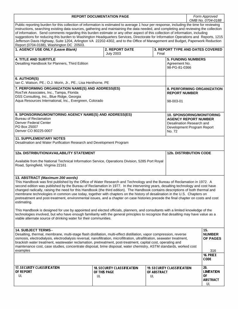
Figures Page 1-1 Growth of global industrial and municipal water consumption...........................................2 1-2 Regional percentages of contracted desalination capacity through the end of 1999 ...........5 2-1 Global desalination capacity for membrane and thermal plants, 1950-2001.....................12 2-2 Global desalination capacity usage, 1950-2001.................................................................12 2-3 Process flow diagram for the Dare County, North Carolina, North RO plant...................17 2-4 Process flow diagram for the Harlingen Reclamation Plant..............................................21 2-5 Ghubrah Complex seawater intake lines............................................................................25 2-6 MSF unit at the Ghubrah Complex....................................................................................25 3-1 Mineral acidity as a function of pH ...................................................................................35 3-2 Effect of bicarbonate alkalinity and CO2 on pH ................................................................35 4-1 General desalting plant schematic – surface supply ..........................................................43 4-2 General desalting plant schematic – ground water supply.................................................44 4-3 Conceptual process design drawing...................................................................................45 4-4 Calcium sulfate solubility ..................................................................................................47 4-5 Multiple effect schematic...................................................................................................51 4-6 MED horizontal tube arrangement.....................................................................................52 4-7 MED process schematic – horizontal tube arrangement....................................................53 4-8 Calcium sulfate solubility and MED operation .................................................................54 4-9 Calcium sulfate solubility and vertically stacked MED operation ....................................54 4-10 MED vertical tube bundle arrangement.............................................................................55 4-11 MED process schematic – vertical tube arrangement........................................................56 4-12 MED vertically stacked tube bundles ................................................................................56 4-13 MED process schematic – vertically stacked tube bundles ...............................................57 4-14 Process schematic, MWD’s short tube test unit.................................................................60 4-15 MSF arrangement...............................................................................................................62 4-16 MSF stage ..........................................................................................................................62 4-17 MSF long tube design ........................................................................................................63 4-18 MSF cross tube design.......................................................................................................64 4-19 MSF schematic, once-through ...........................................................................................64 4-20 MSF recirculation schematic .............................................................................................65 4-21 Calcium sulfate solubility and MSF operations.................................................................66 4-22 VC schematic .....................................................................................................................70 4-23 Mechanical or thermo-compression VC overall process schematic ..................................71 4-24 Calcium sulfate solubility and VC operations ...................................................................71 4-25 ED schematic .....................................................................................................................75 4-26 ED stack assembly .............................................................................................................75 4-27 Examples of hydraulic and electrical staging ....................................................................76 4-28 Three-stage, two-line ED/EDR schematic.........................................................................81 4-29 Osmotic pressure................................................................................................................85

xiv
Table of Contents
Figures Page 4-30 Osmosis and reverse osmosis.............................................................................................86 4-31 Spiral wound element construction....................................................................................89 4-32 Spiral wound membranes and vessel assembly .................................................................90 4-33 Hollow fine fiber permeator schematic..............................................................................90 4-34 Tubular membrane schematic ............................................................................................91 4-35 Plate and frame schematic .................................................................................................92 4-36 Three types of energy recovery devices in use today ........................................................96 4-37 Solute concentration factor as a function of recovery .......................................................97 4-38 Horizontal cartridge filters in Jupiter, Florida ...................................................................98 4-39 Typical chemical feed system............................................................................................99 4-40 Cleaning system, North Hatteras plant, Dare County, North Carolina..............................99 4-41 Simplified RO process flow diagram...............................................................................100 4-42 Typical arrangements for staging.....................................................................................101 5-1 Pretreatment schematic, low temperature design (T = 90 ºC) .........................................108 5-2 Pretreatment schematic, high temperature design (T = 110 ºC) ......................................108 5-3 Langelier Saturation Index nomograph ...........................................................................111 5-4 How a bacterium sticks to the membrane surface ...........................................................116 6-1 Blending mass balance flow diagram ..............................................................................127 6-2 Cross section of typical packed tower .............................................................................129 6-3 HOCl-OCl- equilibrium diagram .....................................................................................132 6-4 Chlorine addition schematic ............................................................................................132 7-1 Process schematic – single-purpose MSF arrangement...................................................142 7-2 Three dual-purpose arrangements – distillation processes ..............................................144 7-3 Dual-purpose arrangement – RO process ........................................................................145 7-4a Relative seawater desalting capital costs (metric) ...........................................................158 7-4b Relative seawater desalting capital costs (U.S.) ..............................................................158 7-5a Relative brackish water desalting capital costs (metric)..................................................159 7-5b Relative brackish water desalting capital costs (U.S.) .....................................................159 7-6a Cost of water seawater desalting (metric)........................................................................160 7-6b Cost of water seawater desalting (U.S.)...........................................................................160 7-7a Cost of water – brackish water desalting (metric) ...........................................................161 7-7b Cost of water – brackish water desalting (U.S.) ..............................................................161 7-8 Energy consumption comparison – RO and EDR ...........................................................164 7-9 BWRO feed pressure versus feed water TDS..................................................................166 8-1 Comparison of concentrate disposal methods for all brackish water processing facilities in the U.S...................................................................................171 8-2 Reclamation’s NEPA flowchart.......................................................................................177 9-1 Total construction cost—MSF process............................................................................207 9-2 Process construction cost—MSF .....................................................................................207 9-3 Total construction cost—MED process ...........................................................................208

xv
Table of Contents
Figures Page 9-4 Process construction cost—MED ....................................................................................208 9-5 Total construction cost—MVC process...........................................................................209 9-6 Process construction cost—MVC....................................................................................209 9-7 Total construction cost—SWRO, BWRO, and NF plants with surface water feed...................................................................................................................210 9-8 Total construction cost—SWRO, BWRO, and NF plants with well water feed...................................................................................................................210 9-9 Total construction cost—EDR plant................................................................................211 9-10 Construction cost—concentrate disposal pipeline for distillation processes...................211 9-11 Construction cost—concentrate disposal pipeline for membrane processes ...................212 9-12 Construction cost—evaporation ponds for membrane processes ....................................212 9-13 Construction cost—injection wells for membrane processes ..........................................213 9-14 Construction cost—pretreatment for distillation processes .............................................213 9-15 Construction cost—surface water pretreatment for membrane processes.......................214 9-16 Construction cost—open intake systems for distillation processes .................................214 9-17 Construction cost—open intake systems for smaller membrane processes.....................215 9-18 Total construction cost—wellfields .................................................................................215 9-19 Construction cost—seawater feed water pipeline for distillation processes....................216 9-20 Construction cost—seawater feed water pipeline for membrane processes....................216 9-21 Construction cost—package boilers for single-purpose plant .........................................217 9-22 Construction cost—site development for distillation processes ......................................217 9-23 Construction cost—site development for membrane processes ......................................218 9-24 Construction cost—post-treatment for distillation processes ..........................................218 9-25 Construction cost—post-treatment for membrane processes ..........................................219 9-26 Construction cost—product storage for distillation systems using steel tank construction........................................................................................................219 9-27 Construction cost—product storage for membrane systems using prestressed concrete tank construction .........................................................................................220 9-28 Construction cost—product transmission pipeline ..........................................................220 9-29 Construction cost—emergency generators ......................................................................221 9-30 Construction cost—step-down transformers....................................................................221 9-31 Construction cost—distillation process buildings ...........................................................222 9-32 Construction cost—membrane process buildings............................................................222 9-33 Owner’s direct expense and COH factors........................................................................223 9-34 Land requirements—for distillation process plants .........................................................223 9-35 Land requirements—for membrane process plants .........................................................224 9-36 Annual cost—labor for distillation process .....................................................................224 9-37 Annual cost—labor for membrane processes ..................................................................225 9-38 Annual cost—MSF chemicals .........................................................................................225 9-39 Annual cost—MED chemicals ........................................................................................226

xvi
Table of Contents
Figures Page 9-40 Annual cost—MVC chemicals ........................................................................................226 9-41 Annual cost—chemicals for surface water membrane processes ....................................227 9-42 Annual cost—chemicals for ground water membrane processes ....................................227 9-43 Annual cost—MSF processes electricity .........................................................................228 9-44 Annual cost—MED processes electricity ........................................................................228 9-45 Annual cost—MVC processes electricity........................................................................229 9-46 Annual cost—SWRO processes electricity .....................................................................229 9-47 Annual cost—BWRO, EDR, and NF plants electricity...................................................230 9-48 Annual cost—steam for single-purpose plants ................................................................230 9-49 Annual cost—steam for dual-purpose plants, power credit method................................231 9-50 Annual cost—steam for dual-purpose plants, available energy method..........................231 9-51 Annual cost—MSF repairs and spares.............................................................................232 9-52 Annual cost—MED repairs and spares............................................................................232 9-53 Annual cost—MVC repairs and spares............................................................................233 9-54 Annual cost—membrane replacement.............................................................................233
Tables Page 2-1 Desalting plant capacity by location, contracted through the end of 2001........................11 2-2 Desalting plant capacity by process, contracted through the end of 2001.........................11 2-3 Typical quality limits for selected industries .....................................................................14 2-4 Ghubrah 1-6 main design features .....................................................................................24 2-5 Ghubrah desalting costs .....................................................................................................24 3-1 Symbols, atomic weights, and common ionic charges commonly occurring in natural waters...........................................................................................32 3-2 Major components of natural water ...................................................................................32 3-3 Analysis of various brackish waters ..................................................................................37 3-4 Typical brackish water analysis .........................................................................................39 3-5 Three methods of reporting water analysis........................................................................40 3-6 Conversion of ionic concentration to CaCO3 equivalents (hardness)................................41 4-1 Process characteristics of MED systems............................................................................58 4-2 Materials of fabrication, MED systems .............................................................................59 4-3 Process characteristics, MSF systems................................................................................67 4-4 Materials of fabrication, MSF systems ..............................................................................68 4-5 Process characteristics, VC systems ..................................................................................72 4-6 Materials of fabrication, VC systems.................................................................................73 4-7 Selected properties of commercial ED/EDR membranes..................................................77 4-8 Pretreated feed water quality goals for EDR .....................................................................82

xvii
Table of Contents
Tables Page 4-9 Typical RO feed pump power consumption ......................................................................94 4-10 Typical recoveries for various vessel lengths ..................................................................101 5-1 Pretreated water quality requirements for membrane processes......................................109 5-2 Typical commercial scale inhibitors ................................................................................113 5-3 Principal events in membrane biofouling processes........................................................115 5-4 Disinfection techniques for biofouling control ................................................................117 5-5 Techniques for removing suspended solids .....................................................................117 5-6 Distribution of hydrogen sulfide species as a function of pH..........................................120 6-1 Effect of mineral addition on water quality .....................................................................125 7-1 Summary of guidelines for desalting selection................................................................136 7-2 Suggested water quality analysis .....................................................................................151 7-3 Unit site areas, for plants of 19,000 m3/d and larger .......................................................152 7-4 Disposal of concentrates ..................................................................................................153 7-5 Data collection checklist ..................................................................................................154 7-6 Plant investment and product water cost for a 37,850 m3/d (10 mgd) MSF base case plant............................................................................................................162 7-7 MSF optimization ............................................................................................................163 7-8 Principal water cost components for ED/EDR ................................................................163 7-9 Principal water cost components for RO .........................................................................165 8-1 Desalination processes and characteristics of their concentrate streams .........................170 9-1 Estimated design and construction periods......................................................................188 9-2 Operations and maintenance staff – distillation processes ..............................................197 9-3 Operations and maintenance staff – membrane processes...............................................198 9-4 Unit costs of chemicals by process and use .....................................................................198 9-5 Capital recovery factors ...................................................................................................201 9-6a Design criteria..................................................................................................................202 9-6b Economic criteria .............................................................................................................203 9-7 Supporting sheet, computation sheet, and cost summary ................................................204

xviii
Acronyms and Abbreviations AMTA American Membrane Technology Association AWWARF American Water Works Association Research Foundation ASTM American Society for Testing Materials BCI Building Cost Index BPE boiling point elevation Btu British thermal unit BWRO brine water reverse osmosis CA cellulose acetate membrane CCI Construction Cost Index CEQ Counsel on Environmental Quality CF concentration factor cm centimeter COH construction overhead CT concentration and time CWA Clean Water Act DBP disinfection byproducts DCC direct capital cost D/DBP disinfection/disinfection byproducts EA Environmental Assessment ED electrodialysis EDR electrodialysis reversal EIS Environmental Impact Statement EPA Environmental Protection Agency ft foot IEC ion exchange capacity g gram gpd gallons per day gpm gallons per minute HAA haloacetic acids HFF hollow fine fiber HMS horizontal multi-stage, with energy recovery turbine hr hour HTC© hydraulic turbocharger kg kilogram kgal thousand gallons kW kilowatt kWh kilowatthour l liter lb pound LSI Langelier saturation index LTTU long tube test unit m meter MED multiple effect distillation meq/g milliequivalent per gram MEW Ministry of Electricity and Water MF membrane filtration

xix
mgd million gallons per day MJ mega joule mm millimeter MSF multi-stage flash distillation MVC mechanical vapor compression MWD Metropolitan Water District of Southern California NA not applicable or not available NDP net driving pressure NEPA National Environmental Policy Act NF nanofiltration NOM natural organic matter NPDES National Pollutant Discharge Elimination System NSF National Sanitation Foundation NTU nephelometric turbidity unit OMB Office of Management and Budget OSW Office of Saline Water PA polyamide membrane PLC programmable control systems ppm parts per million PSD Preventing Significant Air Quality Deterioration psi pounds per square inch psig pounds per square inch gauge PVDF polyvinylidene-fluoride RCRA Resource Conservation and Recovery Act of 1976 RO reverse osmosis RSI Ryznar Stability Index SDI silt density index SDWA Safe Drinking Water Act SRB sulfate reducing bacteria STTU short tube test unit SW spiral wound SWDA Solid Waste Disposal Act SWFWMD Southwest Florida Water Management District SWRO seawater reverse osmosis TDS total dissolved solids THM trihalomethane THMFP trihalomethane formation potential TSS total suspended solids TVC thermo vapor compression distillation UF ultrafiltration UIC underground injection control USGS U.S. Geological Survey UF ultrafiltration U.K. United Kingdom UV ultraviolet VC vapor compression w/ft2-K watts per square foot – degrees Kelvin

Chapter 1: Introduction
1.1 Background
For the purposes of this Desalting Handbook for Planners (Handbook), “desalination” is defined as a water treatment process that removes salts from water. Desalination processes can be used in various applications including:
• Municipal desalting of brackish or seawater for drinking water production
• Industrial and commercial applications for production of high-purity boiler feed water, process water, bottled water, and for zero discharge applications; producing water for industries including the pharmaceutical, electronics, bio/medical, mining, power, petroleum, beverage, tourism, and pulp/paper industries
• Rigorous treatment of wastewater for reuse applications
Desalination has now become an accepted water treatment process around the world and is becoming a price-competitive option for more communities as the cost of desalination is decreasing to the level of new supplies using conventional means.
Fresh water resources on Earth are limited. Over 97 percent of the world’s water is seawater, with an additional 2 percent of the world’s water resources locked up in ice caps and glaciers. Saline ground water and inland saline seas reduce available fresh water even further. As a result, less than 0.5 percent of the Earth’s water resources is available as fresh water for direct human consumption or for agricultural and industrial uses.
Stress on our fresh water resources is increasing as:
• Global population increases • Irrigation and agricultural demands increase • Standards of living improve • Industrialization increases • Environmental needs require more water • Water quality of existing resources declines
Population.⎯The demand for fresh water and population growth are directly related. The world’s population⎯approximately 6 billion people⎯is projected to double in the next 50 to 90 years, while our renewable fresh water resources remain constant. Currently, over 400 million people live in regions with severe water shortages. This is estimated to climb to 2.8 billion people by 2025. This is roughly 35 percent of the projected total population. At least 1 billion of these people will be living in countries facing absolute water scarcity, defined as less than 500 cubic meters (132,000 gallons) per person per year.

Desalting Handbook for Planners
2
Agriculture.⎯Agriculture is the largest single user of our fresh water resources, accounting for approximately 63 percent of the overall water withdrawal worldwide, but over 86 percent of the actual worldwide water consumption. Other water users, such as industry, recycle much of their withdrawal and, therefore, do not consume as much of the water they withdraw. As the population increases, the agricultural demand also increases. Available land for agricultural production is now declining. Raising grain production can only come from higher land productivity, which correlates, in many cases, to increased irrigation.
Standards of living.⎯While overall improvements in standards of living are positive for society, the demand for water resources increases. The domestic consumption rate—as well as the overall per capita consumption—increases with the standard of living of a society. Additionally, an increased standard of living results in the demand for goods and products, which increases industrialization. Water recycling has been effectively applied in many segments of industry, yet consumption for industrial applications continues to climb. Consumption for industrial and municipal use is shown in figure 1-1 for the period 1900 to 2000 to further illustrate our increasing global water demand.
Figure 1-1 Growth of global industrial and municipal water consumption (Gleick, 1993)
In the U.S., particularly, there is a growing desire to ensure environmental water needs are met. Future environmental regulation is expected to ensure that the ecological needs of many rivers, lakes, wetlands, and streams are met by maintaining minimum instream flow requirements, thereby placing additional stress on the multiple and competing users of these bodies of water.
0
5000
10000
15000
20000
25000
30000
35000
1900 1940 1950 1960 1970 1980 1990 2000
Year
Bill
ion
gallo
ns p
er y
ear
Industry Municipal

Chapter 1: Introduction
3
At the same time that water demand is increasing, water quality is diminishing in many parts of the world. The U.S., through the Environmental Protection Agency regulations and programs, has improved its overall water quality over the last two decades. Unfortunately, water quality in much of the rest of the world is still in decline, particularly in Asia and South and Central America. For instance, in China, 82 percent of the rivers are polluted and only 20 percent meet the lowest Chinese government standard for agricultural use. In urban areas of China, 80 percent of the surface water is contaminated. In India, it is estimated that 70 percent of the surface water is severely polluted. Much of this contamination is a result of high industrial activity in densely populated areas with poor environmental regulations, insufficient sanitation in rural and underdeveloped areas, and agricultural runoff contamination.
As water is a precious and irreplaceable resource, water has also been a major source of conflict throughout the world. The Jordan River was at the heart of the 1967 Arab-Israeli conflict, and water issues continue to plague the Middle East peace process. In North Africa, the Nile River is the source of tension between Egypt and Sudan. In south Asia, river waters have been a point of contention between India, Bangladesh, and Nepal. Even in the U.S., water rights between the Western States with access to the Colorado River is contentious, with legal battles and political implications.
Mankind has very limited options by which to reduce these stresses on our water supply. These options include:
• Improved water conservation efforts
• Additional large infrastructure projects (dams, reservoirs, and water carriers and water transfer projects)
• Increased water recycling and reuse of process and wastewater
• Desalination of brackish water and seawater
1.2 Introduction to Desalination Technologies
There are basically two families of desalination technologies used throughout the world today. These include thermal technologies and membrane technologies. Thermal technologies are those that heat water and collect condensed vapor (distillation) to produce pure water. Rarely are distillation processes used to desalinate brackish water (water with less than 10,000 milligrams per liter of total dissolved solids), as it is not cost effective for this application. The thermal technologies include the following specific types of processes:
• Multiple-stage flash distillation (MSF) • Multiple effect distillation (MED) • Vapor compression (VC)—mechanical (MVC) and thermal (TVC).

Desalting Handbook for Planners
4
The concept of distilling water at reduced pressures, as is practiced in the thermal desalination processes, has been used for well over a century, with the early generation of present-day, multi-stage thermal desalters being developed in the 1950s. Thermal desalination is most commonly practiced in areas with abundant fossil fuel that can capitalize on cogeneration of power and water, such as in the Middle East. Membrane technologies use thin, semipermeable membranes to separate the feed stream into two streams of differing concentration, a product and concentrate stream. In desalination applications, the feed is either brackish or seawater. The membrane technologies include the following specific types of processes:
• Reverse osmosis (RO) • Electrodialysis (ED) and electrodialysis reversal (EDR)
The RO process uses pressure as the driving force to separate the saline feed into a product stream and a concentrate stream. The ED/EDR processes use opposing electrodes to separate out the positive and negative ions of the dissolved salts from a saline stream. Nanofiltration (NF) is also a membrane process that is used in some desalting applications, but it principally removes the divalent salt ions (such as calcium, magnesium, and sulfate), not the more common salts (sodium and chloride). As a result, nanofiltration is most commonly used for water softening and other nondesalting applications, such as organics removal. In comparison to thermal processes, membrane technologies are much younger in their development: ED was developed in the 1950s and RO in the 1970s. The membrane market is very fluid—new, improved products are continually introduced to the marketplace. Membrane technologies are generally constructed as single-use facilities, but recent developments indicate synergistic benefits result from co-locating membrane desalination plants with power or other industrial facilities.
1.3 Desalination Market
Thermal and membrane installed capacity contracted through the end of 1999 was approximately 25.74 million cubic meters per day (6.8 billion gallons per day), with 50 percent in distillation capacity and 50 percent in membrane capacity. This capacity has been installed over the history of modern desalination, beginning in the 1950s, and not all of this capacity is presently in operation. Figure 1-2 shows the regional distribution of installed capacity worldwide.

Chapter 1: Introduction
5
Figure 1-2 Regional percentages of contracted desalination capacity through the end of 1999 (Wangnick, May 2000)
On a global basis, the growth rate of desalination capacity from 1972 through 1999 for all desalting technologies averaged just under 12 percent per year, with an average of slightly more than 1.4 million cubic meters per day (370 million gallons per day) additional capacity installed each year. There have been over 8,600 desalination plants installed through 1999, with approximately 20 percent of these in the U.S., 16.6 percent in Saudi Arabia, and 11.2 percent in Japan.
References
Gleick, P., “Water in Crisis – A Guide to the World’s Fresh Water Resources,” Oxford University Press, 1993.
Wangnick, K., “2000 IDA Worldwide Desalting Plants Inventory, Report No. 16,” International Desalination Association, May 2000.
Regional Percentages of Global Desalination Capacity
Middle East47.8%
C.America3.2%
Africa5.5%
Asia12.2%
Europe13.0%
S. America0.7%
N. America17.2%
Australia0.4%


Chapter 2: Desalting Applications
7
Chapter 2: Desalting Applications
Since the early 1970s, desalting has gained a foothold in the U.S. as a practical source of water supply. Desalination is now providing high-quality water for municipal and industrial use, particularly from brackish ground water sources. While most municipal facilities are located in coastal areas, the technology is being used inland in Texas, Colorado, Missouri, Iowa, and elsewhere. The major challenge for inland plants is disposal of the concentrate in a manner that is compatible with the environment.
Along with commercial applications, desalting technology has rapidly advanced, and component life and system reliability have improved significantly. The cost of desalted water, particularly from membrane processes, has declined significantly. Actual experience in full-scale commercial operations and in pilot plants of different types has expanded and will continue to expand the knowledge base. Further improvement in desalting process technology will continue; further reductions in cost will lead to even more growth in desalting as a solution to water supply and quality problems.
Water supply professionals are accustomed to thinking in terms of the hydrologic cycle and how civil works may be applied to the problems of water availability. They have been very successful in using capital-intensive, long-lasting structures, often quite distant from the point of use, in developing water supplies at modest cost to users.
Desalting, by contrast, may be quite independent of the hydrologic cycle and, therefore, free from possible legal or political constraints. Desalting creates new water, as it treats seawater and brackish water. Desalting creates more valuable water, as it increases the utility of brackish water. Additionally, desalting processes can be used in industrial applications to produce ultrapure water or process water of very high quality, thereby greatly enhancing the productivity of numerous industries, including electronics, pharmaceuticals, power, food and beverage, mining, refining, and paper industries.
Desalting plants can generally be located close to the point of use. Desalting adds diversity and, therefore, insurance to a water system because it is fundamentally different from the conventional water sources that it might complement. Desalting requires less investment per unit capacity than conventional water treatment facilities, particularly to acquire the source water. However, desalting may have higher operating costs. Desalting capacity is available in a variety of plant sizes and processes and can be matched closely to the water demand curve, possibly making an investment in desalting more suitable for financing than a capital and environmentally intensive conventional water project. Desalting is a hardware technology, and continued improvements in its efficiency are expected. Prototype plants will provide experience in large plant operation. Continued research and development will bring process efficiencies closer to theoretical limits.

Desalting Handbook for Planners
8
2.1 Sources of Feed Water
Because desalting converts saline waters into a resource, the technology has broadscale application where water has high value. Source waters include ocean waters and numerous inland sources of saline water, such as geothermal, brackish ground and surface water, and wastewater.
2.1.1 Industrial Wastewater
Industrial use of reclaimed wastewater for cooling water and processes has increased in recent years. Applications currently include power plant and refinery cooling water and process water in such industries as textiles, electronics, and pulp and paper. A 15,142 cubic meters per day (m3/d) (4 million gallons per day [mgd]) plant in Harlingen, Texas, provides high-quality water “across the fence” to a Fruit of the Loom facility. Conventional water sources were unable to supply the quantity required, but using wastewater reclaimed with reverse osmosis (RO) provided the necessary quantity, at a much higher level of quality. The major outcome of this project was the creation of 2,000 manufacturing jobs in largely agricultural southeast Texas.
2.1.2 Municipal Wastewater
Municipal reuse is a potential application of water renovation programs. Multiple barriers are required for both direct and indirect reuse of reclaimed municipal wastewater. Desalting is a necessary step in treating wastewater for reuse when salinity exceeds certain levels. Treated water may be suitable for ground water recharge or for industrial and agricultural use.
The use of reclaimed municipal wastewater for nonpotable use has increased dramatically over the past 25 years. The first and, possibly, best known example of the use of desalting technology to meet ground water recharge rules is Water Factory 21 in Fountain Valley, California. A system involving a 18,927 m3/d (5 mgd) reverse osmosis plant has been in operation since 1977, treating secondary effluent to a high level of quality prior to injecting it into the local ground water system, both as a salinity barrier and for recharge. In this case, the membrane treatment is used to reduce total dissolved solids (TDS) and to provide a barrier against dissolved organic matter and pathogens. Currently, a 283,906 m3/d (75 mgd) system is under design, which will combine both membrane filtration and RO to treat secondary effluent for discharge into the Santa Anna recharge areas.

Chapter 2: Desalting Applications
9
2.1.3 Brackish Ground Water
In water-short areas, even brackish water may be used as a public water supply source, either by itself or mingled with other, better water to satisfy user needs. The use of brackish water also often presents problems involving water rights.
Because each source of brackish water is unique, thorough investigation is necessary to determine the optimum process design for that site. Most brackish water can be reclaimed by membrane-type plants because the salinity is low in comparison to seawater.
Unlike seawater, the quantity of brackish ground water is often limited. Thus, detailed investigation of the aquifer by test wells and modeling should always be conducted—especially when the source to be used has not previously been exploited. Key factors in the hydrogeological work are the safe yield, long-term storage, and proclivity for significant changes in the water chemistry. The latter should not be limited to increases in TDS, but also possible changes in ionic distribution with time.
Maps of the 20 hydrologic regions of the U.S. are available from the U.S. Geological Survey (USGS); the USGS has performed ground water studies in almost all of the U.S. In addition, some States have made independent ground water surveys, and many States now require ground water pumping permits. Such permit applications often require the applicant to perform the necessary hydrogeological studies as part of the permit application.
2.1.4 Brackish Surface Water
In recent years, there has been an increasing interest in using brackish surface waters as a source of potable water, particularly in areas where traditional sources of fresh water are limited in capacity or are being stressed by competing uses, such as irrigation and industrial needs. The source of these waters may be either naturally brackish (such as the Brazos River and Lake Granbury in Texas) or from an estuary (where river waters meet tidal waters). The RO plant in Robinson, Texas, uses water from the Brazos River as its feed water, while Lake Granbury provides water to an electrodialysis reversal (EDR) plant operated by the Brazos River Authority.
The advantage of surface water supplies over brackish ground water is that, generally, surface water supplies are not limited, except in severe cases of drought, when fresh water flows into the system may be depleted. In such instances, the salinity of the feed water may increase beyond the ability of the desalting plant to produce potable quality water.
Pretreatment also becomes more complicated with surface water as feed water because suspended solids, biological activity, and pathogens must be addressed prior to the desalting operation. In addition, the Surface Water Treatment Rule of the Safe Drinking Water Act must

Desalting Handbook for Planners
10
be considered in planning these types of facilities. The use of membrane filtration as pretreatment addresses most, if not all, of these issues.
2.1.5 Seawater
Coastal locations present a virtually unlimited source of water of reasonably uniform quality and composition, as well as a convenient and economical sink for disposing concentrate. Also, dual-purpose plants for power and water production are best located near an unlimited supply of cooling water. Using seawater as a source is usually indicated when the point-of-use is located in or near coastal areas. Desalted seawater can also be used to supply areas a considerable distance from the coast, as in Saudi Arabia. The distance that desalted water can be conveyed is, of course, limited by the cost of constructing and operating the conveyance system. In some areas, it may be possible to supply additional water to areas far removed from the coast by exchange of desalted water for river water. For example, studies by the Bureau of Reclamation for augmentation of the Colorado River in the Yuma, Arizona, area showed that supplying desalted seawater or brackish water either to the metropolitan Los Angeles area, or to the Lower Colorado River area near Yuma, could, by exchange, make water available in the Upper Colorado Basin, more than 1,000 miles from the desalting areas.
2.2 Desalting for Water Supply
Approximately 8,700 land-based desalting plants had been installed or contracted for installation throughout the world by the end of 1999. These plants have a capacity above 100 m3/d or 26,400 gallons per day (gpd). Worldwide installed capacity in 1999 was 25.74 million m3/d (6.8 billion gpd). Distillation accounts for about 50 percent of worldwide desalting capacity, with multi-stage flash (MSF) distillation providing about 84 percent of that quantity. Membrane technology accounts for the remaining 50 percent of the worldwide desalination capacity, with RO contributing 83 percent of that quantity.
The following graphs and tables are statistical summaries of data contained in Desalting Plants Inventory Report No. 16, published by Wangnick Consulting Gmbh (Wangnick, May 2000). Table 2-1 lists the number of land-based desalting plants by location; table 2-2 lists the number of plants by process. Figure 2-1 shows that desalination capacity has significantly increased since the early 1970s. In addition, it shows that the use of thermal and membrane technology is about equal. Figure 2-2 illustrates the global water usage of desalination technology by user type over the last 50 years. Figure 2-2 indicates that since the early 1970s, industry and municipalities use more desalinated water than the military and power producers.
2.2.1 Supplemental Public Supplies in the U.S.
Approximately 150 U.S. municipal water systems use desalting for a part or all of their supply. Approximately 94 percent of this capacity is generated using membrane technology.

Chapter 2: Desalting Applications
11
Together, these processing facilities produce over 2.98 million m3/d (787 mgd) of water for municipal use.
Table 2-1.—Desalting plant capacity by location, contracted through the end of 2001
Region
Number of plants
Installed capacity, m3/d (mgd)
United States 1,863 5.129 x 10⁶ (1,355)
Central America 167 0.399 x 10⁶ (106)
Canada/Bermuda 69 0.082 x 10⁶ (22)
Caribbean 240 0.741 x 10⁶ (196)
South America 142 0.261 x 10⁶ (69)
Europe 1,572 4.182 x 10⁶ (1,104)
Africa 786 1.662 x 10⁶ (439)
Middle East 2,470 15.855 x 10⁶ (4,189)
Asia 1,994 3.625 x 10⁶ (958)
Australia 134 0.239 x 10⁶ (63)
Russia 32 0.125 x 10⁶ (33)
Unknown 41 0.071 x 10⁶ (19)
Total - all locations 9,510 32.373 x 106* (8,553)
(Individual region totals do not add to 25.89 x 10⁶ because of rounding.)
Table 2-2.—Desalting plant capacity by process, contracted through the end of 2001
Process
Number of plants
Plant capacity, m3/d (mgd)
Multi-stage flash distillation 667 12.727 x 10⁶ (3,363)
Vapor compression 652 1.549 x 10⁶ (409)
Multi-effect distillation 428 1.028 x 10⁶ (272)
Reverse osmosis 6,463 14.100 x 10⁶ (3,725)
Electrodialysis/electrodialysis reversal 997 1.533 x 10⁶ (405)
Nanofiltration 44 1.230 x 10⁶ (325)
Other 259 0.206 x 10⁶ (54)
Total - all types of processes 9,510 32.373 x 10⁶ (8,553)

Desalting Handbook for Planners
12
Figure 2-1 Global desalination capacity for membrane and thermal plants, 1950-2001
Figure 2-2 Global desalination capacity usage, 1950-2001
Desalination Capacity Usage Distribution
Municipal
Industrial
Power
Military
Tourism
Other
Global Desalination Capacity
0
500
1000
1500
2000
2500
3000
3500
4000
4500
5000
1950
1953
1956
1959
1962
1965
1968
1971
1974
1977
1980
1983
1986
1989
1992
1995
1998
2001
Year
Cum
ulat
ive
Cap
acity
(Mgd
) MembraneThermal

Chapter 2: Desalting Applications
13
Municipal benefits, such as dependability and a consistent, high-quality supply, are making desalination attractive to a variety of municipalities. The choice of the best process for each case will depend principally on local water conditions, water quality, energy costs, and concentrate disposal options.
Desalination processes have grown significantly in the past few years. Further improvements, particularly in continued reduction of energy requirements and in-process performance, are being pursued by manufacturers and through government-sponsored research, development, and demonstration.
2.2.2 Alternative to Reservoir Development
A desalting plant may be an attractive alternative to a "last added" reservoir in a system when increased firm yield is desired. The last added reservoir may be a marginal investment in terms of dollars per unit yield of water. In contrast to the reservoir, desalting has a lower capital investment, but it trades capital cost for higher operating cost. Additionally, the environmental impact from a desalting facility is much less than adding additional reservoir capacity.
Alternatively, conjunctive use of reservoirs and desalting facilities can provide the water resource planner a useful economic model. A desalting plant can be matched to the water demand curve, in modular fashion, much more closely than a dam and reservoir because a dam is most economically constructed by relation to the site and stream hydrology, rather than to the demand curve. A desalting plant may be more financially desirable. Because the desalting plant is less capital intensive, it may be easier for the water supply agency to obtain financing. In times of higher interest rates, the desalting plant may be a more feasible investment.
2.2.3 Alternative to Long-Distance Water Transfer
Desalination plants are usually close to the point of water use. Therefore, desalted water supply probably will have a much shorter lead time than long-distance water transfer. Additionally, a desalting facility will often have less environmental impacts than a long-distance pipeline.
2.2.4 Industrial Applications
Specifications for industrial water purity vary widely and depend entirely on the intended use. Highly saline water is often acceptable for cooling and condensing industrial exchangers. On the other hand, requirements for pure process water are so stringent in many industries that plants often employ expensive and complex treatment for even high-quality natural water.
No formal quality standards exist for an entire industry, or even for specific products, although estimates of quality tolerances by industries are available in various reports. One such set of limits is given in table 2-3.

Desalting Handbook for Planners
14
Table 2-3.—Typical quality limits for selected industries (mg/l)
Industry Turbidity Color Hardness Alkalinity pH TDS Fe and Mn
Baking 10 10 0.5
Boiler feed
0-150 psi 20 80 75 8.0+ 1,000-3,000
150-250 psi 10 40 40 8.5+ 500-2,500
250-400 psi 3 5 8 9.0+ 100-1,500
>400 psi 1 2 2 9.5+ 50
Brewing
Light 10 75 6.5-7 300 0.1
Dark 10 150 7.0+ 1,000 0.1
Canning
General 10 0.2
Legumes 10 25-75 0.2
Carbonated beverages
2 10 250 50 850 0.3
Confectionary 50 100 0.2
Cooling 50 50 0.5
Icemaking 1-5 5 30-50 300 0.2
Laundering 50 0.2
Clear plastics 2 2 200 0.02
Pulp and paper
Ground wood 50 20 180 1.0
Kraft 25 15 100 300 0.2
Soda and sulfite 15 10 100 200 0.1
Light paper 5 5 50 200 0.1
Rayon (viscose)
Production 5 5 8 50 100 0.05
Manufacturing 0.3 55 7.8-8.3 0.0
Tanning 20 10-100 50-135 133 8.0 0.0
Textiles
General 5 20 20 0.25
Dyeing 5 5-20 20 200 0.25
Wool scouring 70 20 1.0
Cotton bandage 5 5 20 0.2
Note: psi = pounds per square inch; mg/l = milligrams per liter

Chapter 2: Desalting Applications
15
Much of the water used in the textile, leather, paper, chemical, and food industries has to have very low hardness and low salinity. Water used in the manufacture of textiles and high-grade paper also requires extremely low iron content. With textiles and carbonated beverages, water must be sparkling, free of organic and inorganic suspended matter, clear, and relatively free of dissolved minerals, especially calcium and magnesium. Process water used in the electronics and pharmaceutical industries must be free of ions and contaminants.
The most common industrial water quality problems are caused by suspended solids and hardness. Both problems respond to relatively inexpensive treatment by conventional methods. However, when other constituents are included, distillation or selective ion exchange processing of part or all of the water supply may be a desirable and economical solution. An example of a very high water quality need is in supercritical power plants. One such plant, with temperatures of 659 oC (1,200 °F) and pressures of 345 bar (5,000 psi) has the following feed water maximums:
2.3 Case Histories
To demonstrate both the necessity of alternative water sources and the usefulness of desalting technology in meeting that need, four site-specific studies have been provided. Each study includes a description of water needs and constraints in each geographic area. In addition, each study illustrates the implementation of desalting technology and includes a process flow diagram and description for the process facility. Finally, each study contains an economic summary of the cost of these technologies for each case.
2.3.1 Brackish Water Desalting using Reverse Osmosis
Location.—Dare County, North Carolina
Background.—The Dare County Water Department, the community, and its governing boards made the decision to use desalination in the mid-1980s, prompted by the need for consistently available, potable-quality water to strengthen the economic growth and financial well-being of the county.
Total dissolved solids 0.50 mg/l
Silica 0.02 mg/l
Iron 0.01 mg/l
Copper 0.01 mg/l
Dissolved oxygen .005 mg/l
pH 9.5 to 9.6

Desalting Handbook for Planners
16
The Outer Banks of Dare County, North Carolina, have almost no fresh water resources. Limited treated water is available from a 18,925 m3/d (5 mgd) ion exchange treatment plant on Roanoke Island, supplemented in the summer by a small fresh water pond providing an additional 3,785 m3/d (1 mgd). This total capacity of 22,710 m3/d (6 mgd) was insufficient to spur economic growth in the area, particularly that afforded by summer tourism and recreation. In addition, further withdrawals from the fresh water aquifer on Roanoke Island were not possible.
When desalination of brackish water sources on the islands was proposed in the 1980s, it was considered quite an expensive alternative. The value of good quality water in terms of retail and commercial success, tax revenues to support services that benefit the residents, and the overall quality of life all determined that the benefits provided by desalination outweighed the cost, even in 1980 dollars. The first plant was in operation by 1989. As the cost of desalination has declined in the 1990s, additional desalination plants were brought online in 1996 and 2000.
The most significant benefit of this project has been the economic growth afforded by the availability of potable-quality water. Growth in total retail sales is one of the most useful indicators of development and economic activity. In Dare County, total retail sales increased from $216 to $800 million from 1984 to 1998. Over the last 10 years, retail sales have increased an average of more than 8 percent per year. Over this same period, the growth in retail sales in Dare County has exceeded the growth rate of the State of North Carolina by more than 7 percent and exceeded the second ranked county in total retail sales by 30 percent.
The assessed value of property within Dare County has grown 148 percent over the last 10 years, while the per capita income of permanent residents has grown almost 35 percent over this same period. While it is difficult to totally credit this economic boon to the advent of desalination in Dare County, it is safe to say that this level of growth would not have been possible without the consistent availability of high-quality water. The technology did not inhibit financial success of the area but, rather, acted as a catalyst for growth and prosperity.
Project Overview.—The Dare County desalination plants are located on the Outer Banks of North Carolina, within the community of Kill Devil Hills and on Hatteras Island. Three desalination plants are in operation, with a small fourth plant under construction in the mainland community of Stumpy Point. Currently, the Dare County water system has a 20,439 m3/d (5.4 mgd) desalination capacity, serving 25,000 permanent residents and a summer population of over 100,000 visitors.
The Dare County desalination plants all use RO technology. The first plant, the North RO plant, in operation since 1989, is a 11,355 m3/d (3.0 mgd) plant, located in Kill Devil Hills. An additional 3,785 m3/d (1.0 mgd) plant began operation in 1996 on northern Hatteras Island, and another 5,299 m3/d (1.4 mgd) began operation in 2000, serving south Hatteras Island. Figure 2-3 describes the technology used at the Kill Devil Hills facility. The Kill Devil Hills facility treats brackish water from local wells using RO technology that has a recovery of 75 percent.

Chapter 2: Desalting Applications
17
Figure 2-3 Process flow diagram for the Dare County, North Carolina, North RO plant
Costs and Conclusions.—Dare County Water Department uses a combination of desalinated water from its three desalination plants, in addition to the older, conventional ion exchange treatment plant on Roanoke Island, to meet its water demand. Overall production is distributed between the plants to minimize costs, with 54 percent of the water supply originating from the desalination plants over the past 9 years. The plants on Hatteras Island serve separate communities and are not connected to each other or to the Roanoke Island and North systems.
Dare County Water Department has conducted a thorough cost comparison of its desalinated supply and its conventional supply, determining that the cost to produce (without depreciation) desalinated water is less than that of the conventional supply. Since 1995, the desalinated water has cost less than $0.40 per cubic meter (m3) ($1.50 per thousand gallons [kgal]), with the cost decreasing each year. Electrical costs average $0.06 per kilowatthour (kWh) (204.76 British thermal units [Btu]) in this area. Dare County Water Department has negotiated a load management plan with the power company, so that power cost at the Kill Devil Hills plant consistently averages below $0.045/kWh (153.57 Btu).
As desalination water costs have declined and the community has prospered as a result of the availability of high-quality water, it is clear, in retrospect, that desalination has been the right approach.
2.3.2 Seawater Desalting using Reverse Osmosis
Location.—Tampa, Florida
Background.—Tampa Bay Water is Florida’s largest water wholesaler, providing water to its member governments of Hillsborough, Pasco, and Pinellas Counties, and the cities of New Port
Brackish feed from wells
Acidification & Scale Inhibition
Cartridge Filtration
RO Variable Speed Pump
1st Stage RO Storage
Effluent to Atlantic Ocean
Post-treatment
2nd Stage RO

Desalting Handbook for Planners
18
Richey, St. Petersburg, and Tampa. Those member utilities, in turn, serve 2 million people in the Tampa Bay area. Tampa Bay Water, in partnership with Poseidon Resources, Tampa Electric, and the Southwest Florida Water Management District (SWFWMD), is presently developing the nation’s largest seawater desalination plant, initially producing 94,625 m3/d (25 mgd) of potable water.
The tri-county area, like many coastal cities, has experienced significant growth in recent years. Overpumping at the well fields has created environmental stresses. SWFWMD mandated that Tampa Bay Water reduce ground water pumping from a current level of 598,030 m3/d (158 mgd) to 457,985 m3/d (121 mgd) by 2003. Additionally, by the year 2008, the pumping must be further reduced to 340,650 m3/d (90 mgd). To address this significant reduction in ground water pumping, a Master Water Plan was developed for the community, which will use seawater desalination to provide 10 percent of the total water supply by the year 2007.
Though desalination, especially seawater desalination, has historically been too expensive for most U.S. communities, the economics are changing. The desalination technologies used today are cost effective and dependable, with improved energy efficiencies, manufacturing, and material improvements contributing to the improved economics. At the Tampa Bay plant, additional cost savings were realized though a public/private partnership and collocation with an electric utility. Tampa Bay Water has chosen desalination as a drought-proof, cost-effective means to diversify its water supply.
The most significant benefits of this project will be:
• The protection of the environment by reduction in well field pumping from the ground water aquifers
• Continued economic growth and prosperity of the community from the ongoing availability of high-quality water for human consumption, tourism, and industry
Additionally, the project will generate about $162 million in direct economic benefits to Hillsborough County in wages and personal income, with total project revenue of about $600 million to the community.
Project Overview.—The Tampa Bay Water plant will initially produce 94,625 m3/d (25 mgd) of drinking water, expandable to 132,475 m3/d (35 mgd). Seawater will be taken from the adjacent Big Bend Power Plant, which uses seawater as a process coolant. The recovery for this desalination process is expected to be approximately 57 percent, and the concentrate stream will be blended with cooling water before it is discharged into the bay. The concentrate stream will have more than twice the salinity of the feed stream. Approximately 71,915 m3/d (19 mgd) of concentrate will be mixed with 5.3 million m3/d (1,400 mgd) of power plant cooling water in order to reduce the salinity of the concentrate stream and ensure that the marine ecosystem will not be affected by the discharge.

Chapter 2: Desalting Applications
19
Environmental Considerations.—Tampa Bay Water and its member governments, along with SWFWMD, were very sensitive to the needs of the aquatic life and marine environment in Tampa Bay and conducted several studies on the bay. One of the reasons for selecting the Big Bend Power Plant site is the volume of data available to predict any changes that might occur once the plant is operational. In addition, this site provides the ability to mix the discharge from the power plant and desalination plant concentrate flow before returning it to the bay. Though all predictions indicate there will be no effect on the Tampa Bay marine environment, a lifetime monitoring program will ensure that if there are any impacts, they will be identified and operations will be changed accordingly.
Costs and Conclusions.—The desalination plant will cost approximately $100 million to construct. The plant is a public/private partnership with the private partner, Tampa Bay Desal, LLC. Tampa Bay Desal, 100 percent owned by Poseidon Resources, will incur much of the financial risk for the project. Additionally, the SWFWMD is co-funding the project to offset the cost to Tampa Bay Water. As a result, Tampa Bay Water will pay only a 30-year net average of $0.55/m3 ($2.08/kgal) of desalinated water, less the $0.11 - 0.16/m3 ($0.40 - 0.60/kgal) using the SWFWMD funds towards the capital cost of the plant. Final cost to Tampa Bay Water customers is about $0.42/m3 ($1.60/kgal).
The cost for seawater desalination for the Tampa Bay Water project is low, when compared to historical seawater desalination costs in other parts of the world. The low cost can be attributed to the lower salinity of the Gulf seawater compared to seawater in many other areas, shared intake/outfall with the Big Bend Power Plant, reasonable power cost of $0.04/kWh (136.51 Btu), and improved economics through a long-term public/private partnership and financial support of SWFWMD.
2.3.3 Wastewater Reclamation using Reverse Osmosis
Location.—Harlingen, Texas
Background.—Harlingen, Texas, is a predominantly agricultural community of approximately 55,000 inhabitants, located near the southern tip of Texas, about 10 miles from the international border with Mexico. High unemployment rates in the 1980s and early 1990s prompted the community to create the Harlingen Development Corporation to organize and support industrial development in the area.
The first obstacle for the Harlingen Development Corporation in attracting new industry to the Harlingen area was the lack of available new water. In 1988, the Harlingen Water Works System commissioned a study to determine the most cost-effective method to provide water and wastewater service to a potential industrial customer. The results of that study indicated only three options were available:
• Buy existing potable water supplies, followed by further treatment to meet water quality criteria. Finding willing sellers was difficult, and water was expensive.

Desalting Handbook for Planners
20
• Use irrigation canal returns and treat extensively, although quality and quantity were unreliable.
• Use domestic wastewater and treat extensively (water reuse).
Cost estimates at the time the study were conducted, which indicated production costs for each of the three options:
$/m3 $/kgal
Potable source (Option 1) 0.44 $1.65
Irrigation canal (Option 2) 0.30 $1.15
Water reuse (Option 3) 0. 023 $0.88 As a result of the preferred economics of reuse, the reliability of the flow, and the conservation aspects of this source of water, water reuse was chosen as the preferred option. Reuse of the industrial wastewater return from the Fruit of the Loom plant was not included in the initial phase of the project but is being considered for future use.
The Harlingen Water Works System, a city-owned and board-operated corporation that provides water and waste treatment services to the city, determined that treating domestic wastewater was the most cost-effective method to provide additional water supplies to potential industrial customers, based on the options available. The industrial partner, Fruit of the Loom Corporation, agreed to locate a major facility in Harlingen if at least 6,056 m3/d (1.6 mgd) of water were available for its use. The Harlingen Reclamation Plant began its successful operation in 1990, providing water to the adjacent Fruit of the Loom plant. Supplemental plant expansions since that time have brought the total capacity of this facility to 15,140 m3/d (4 mgd), of which 11,355 m3/d (3 mgd) is currently used.
The most significant benefits of this project have been:
• Creating approximately 3,000 jobs in a community of high unemployment
• Demonstrating on a national level the value, benefit, and successful economics of water reuse, even for small communities
Project Overview.—The Harlingen Reclamation Plant has been constructed in phases to meet the growing needs of the community. The initial phase, which began operation in 1990, produced 8,327 m3/d (2.2 mgd), using only municipal wastewater as feed water. A follow-on expansion, completed in 1999, added capacity up to about 15,140 m3/d (4 mgd), of which 11,355 m3/d (3 mgd) is currently used. The production from this facility is limited by the available wastewater feed, which is currently all municipal wastewater. Future plans to use industrial wastewater from the adjacent Fruit of the Loom plant could bring the plant into its full 15,140 m3/d (4 mgd) capacity.

Chapter 2: Desalting Applications
21
The plant uses extensive conventional pretreatment prior to its RO system. Figure 2-4 shows the flow diagram of the technologies used at the Harlingen facility.
Figure 2-4 Process flow diagram for the Harlingen Reclamation Plant.
The facility discharges the waste stream through the Arroyo Colorado, which is a tidally influenced creek that eventually discharges into the estuary of the Rio Grande River. The RO discharge is mixed with the treated wastewater discharge from Fruit of the Loom, which is not being reused, to dilute the salt content of the concentrate prior to discharge.
The Harlingen plant has operated successfully for more than 10 years, with an on-line factor of greater than 90 percent. Continued economic growth and water deficiencies in the area may dictate further expansion and continued technological improvements in this proven leader.
Costs and Conclusions.— Federal and State grants were obtained to assist in constructing the initial project. State loans provided additional financial resources for the project. Water costs for this reused source average $0.23/m3 ($0.87/kgal), with the potential for future reductions as the plant implements new, more cost-effective technologies.
The Harlingen experience has been an excellent example of how a community can improve its economic standing through creative solutions to water resources development. Bringing a strong industrial customer to the community, with potential for future growth, has played a significant role in the economic well-being of a community susceptible to drought impacts from its strong agricultural base. Water reuse has played an integral role in meeting this community’s needs, and their circumstances are not unique. More communities are considering and utilizing reuse, as water demands grow and supplies remain constant or are declining.
Two - stage filtration Reverse Osmosis
Storage
Bar Screens
Primary Clarifiers
Trickling Filters
Bio-Towers
Solids Contact Chamber
Flocculating Clarifiers
Chlorine Contact
Industrial Waste

Desalting Handbook for Planners
22
2.3.4 Seawater Desalting using Multi-Stage Flash
Location.—Ghubrah Complex, Muscat, Oman
Background.—Desalting in the Sultanate of Oman came later than in most of the Arabian Gulf States, with the first municipal seawater desalting plant becoming operational in 1976. Almost all the thermal desalination facilities producing water for municipal use in the Middle East region are developed in phases. That is, a desalting complex is developed in phases over time, as capacity is needed and as the financing is available. The Ghubrah Complex near Muscat, Oman, consists of six MSF “plants” or phases, which have been put into service starting in 1976 through 2000. Four of these plants were supplied by the same Japanese manufacturer, while the other two were supplied by German and United Kingdom (U.K.) suppliers. Like most thermal desalination plants, the Ghubrah Complex is a cogeneration facility, producing both electrical power and desalinated water. The facility currently can produce approximately 189,250 m3/d (50 mgd) of desalinated water and 630 megawatts of electricity.
The country of Oman has significantly more renewable water resources than its neighbors, with about 761 m3 per capita per year (201,000 gallons per capita per year), based on year 2000 populations, while the United Arab Emirates has less than 204 m3 per capita per year (54,000 gallons) per capita per year, and Kuwait has less than 83 m3 (22,000 gallons) per capita per year. These renewable water resources are accessed through reservoirs located throughout the country, and they greatly offset the dependency on seawater desalination in Oman. Additionally, Oman is generally conservative with its water resources and relies heavily on water recycling for nonpotable needs, particularly in the more urban greater area of Muscat. During the mid-1970s, however, as the greater Muscat area was modernizing, the demand for water and electricity increased dramatically and outpaced their renewable water resources. The decision to construct the Ghubrah desalination/power facility resulted.
Desalinated water in Oman is the responsibility of the Ministry of Electricity and Water (MEW), and the MEW is responsible for the Ghubrah Complex. The complex is operated by SOGEX, a private company. The original MSF unit, Ghubrah 1, produced approximately 22,710 m3/d (6 mgd) of desalinated water. Subsequent additions resulted in the following overall production capacity for this complex:
Ghubrah 1 22,710 m3/d (6.0 mgd) Ghubrah 2 27,252 m3/d (7.2 mgd) Ghubrah 3 54,505 m3/d (14.4 mgd) Ghubrah 4 27,252 m3/d (7.2 mgd) Ghubrah 5 27,252 m3/d (7.2 mgd) Ghubrah 6 31,794 m3/d (8.4 mgd) Total 190,764 m3/d (50.4 mgd)

Chapter 2: Desalting Applications
23
Project Overview.—The intake for the Ghubrah desalination plants extends 1.0 kilometer (0.6 mile) into the Gulf of Oman. Seawater is drawn by vacuum through 203-centimeter (80-inch) pipes into a seawater pump pit, located adjacent to the beach on the plant site. Figure 2-5 is a photograph of the intake line. Centrifugal pumps bring the water into the plant from this location for distillation.
Each of the seven distillation units (Ghubrah 3 consists of two units) at the Ghubrah Complex are MSF units. The initial unit installed at Ghubrah 1 is significantly different in design from the subsequent units. Unit 1 uses a long tube, parallel flow-type evaporator, while the subsequent units use cross-tube evaporators. Additionally, Unit 1 employs three blowdown pumps. On all other units, the blowdown is taken from the discharge line of the concentrate pump. All units utilize concentrate recirculation. Table 2-4 summarizes the design data for the seven Ghubrah units, and figure 2-6 is a photograph of one of the Ghubrah MSF units.
The Ghubrah Complex is operated in four different modes, with steam from:
• Turbine extracts • Back pressure turbine • Waste heat recovery boilers directly • Fired boilers directly
Power demand greatly fluctuates between summer and winter, whereas the water demand is relatively constant year-round. As a result, in summer, the power and desalination plants are run at full load; while in winter, the power plants are run at low loads and the desalination plants are run at full load. The Ghubrah plants are designed to accommodate these variations in electric load without significant variation in water demand. At low electrical loads, exhaust heat can supply only part of the energy needed for desalination, and the balance is provided directly from the boilers. As a result, the energy cost allocated to desalting increases in the winter.
The desalinated water is stabilized before distribution or storage by passing it through a limestone bed. The water can be stored in onsite reservoirs prior to distribution to the city of Muscat. The final product water fully meets the Omani drinking water standards.
Costs and Conclusions.—The Ghubrah Complex has efficiently provided desalinated water and electricity to the Muscat area for over 25 years. It has made possible the transformation of the area from a walled city without paved highways to a modern industrialized city with all the conveniences of any contemporary municipality.
Each of the phases of the Ghubrah Complex vary in their cost of operation, due to their differences in design and mode of operation relative to the power plant. Because the boilers must be direct fired in the winter to provide sufficient steam for the MSF process, the plants are significantly more costly to operate in the winter. During the summer, more waste heat is available, due to the heavier loads on the power plant, thereby decreasing the cost allocation of fuel to the distillation process. Table 2-5 presents the costs of fuel and other costs (including auxiliary power, manpower, consumables, spare parts, depreciation, and chemicals) for the summer and winter period, for an average of all phases of the Ghubrah Complex.

Desalting Handbook for Planners
24
Table 2-4.—Ghubrah 1-6 main design features Item Ghubrah 1 Ghubrah 2 Ghubrah 3 Ghubrah 4 Ghubrah 5 Ghubrah 6
Type and year of installation
Long tube 1976
Cross tube 1982
Cross tube 1986
Cross tube 1992
Cross tube 1996
Cross tube 2000
Capacity, mgd 6 (22,720 m3/d)
7.2 (27,252 m3/d)
2 x 7.2 (54,504 m3/d)
7.2 (27,252 m3/d)
7.2 (27,252 m3/d)
8.4 (31,794 m3/d)
Gained output ratio, pounds dist./pounds condensate
6.8 (3.08 kg)
6.42 (2.91 kg)
6.42 (2.91)
6.52 (2.96)
Unknown Unknown
Distillate quality, parts per million
100 50 50 50 50 50
Design inlet temperature, ºC
Max.35 30-35 30-35 30-35 30-35 30-35
Seawater -tempering system
Not provided Duplex seawater recirculation pumps
Seawater supply pump with tempering falling in the suction pit
One seawater recirculation pump
Unknown Unknown
Make-up strainers
Not provided Duplex strainers system
Blowdown system
Triplex pumps From discharge of concentrate pumps
Vacuum system Steam ejectors + direct mixing barometric condensers
Shell and tube vent condenser + steam ejectors + shell and tube inter- and after-condensers + condensate extraction pumps
Control station Remote control room + plant- side condensers
Remote control room + local control room + plant side control
Remote control room + plant side control
Unknown Unknown
Number of main closed control loops
7 12 12 13 Unknown Unknown
Number of main open control loops
2 13 12 12 Unknown Unknown
Chemical dosing system
Antiscale, antifoam sodium hydroxide (NaOH)
Antiscale, antifoam, sodium hydroxide (NaOH) sodium sulfite
Table 2-5.—Ghubrah desalting costs Summer Winter
Cost of fuel, $/m3 ($/kgal) 0.073 (0.275) 0.284 (1.075) Other costs, $/m3 ($/kgal) 0.563 (2.130) 0.599 (2.266) Total costs, $/m3 ($/kgal) 0.636 (2.405) 0.883 (3.341)

Chapter 2: Desalting Applications
25
Figure 2-5 Ghubrah Complex seawater intake lines
Figure 2-6 MSF unit at the Ghubrah Complex

Desalting Handbook for Planners
26
References
Wangnick, K., “2000 IDA Worldwide Desalting Plants Inventory, Report No. 16,” International Desalination Association, May 2000.

Chapter 3: Water Chemistry
27
Chapter 3: Water Chemistry
3.1 Basic Water Chemistry
Knowing water chemistry is necessary to:
• Interpret chemical analyses of saline waters • Understand the chemical reactions associated with the desalting processes • Select appropriate pretreatment and post-treatment techniques
Some fundamental concepts of general chemistry must be discussed along with the specific aspects of water chemistry. The general chemistry, water chemistry, and electrochemistry background in this section provides the basis for the further discussions on water types and treatments in section 3.2 and for the various desalting processes and pretreatment methods discussed later in this Handbook.
3.1.1 Water Cycles and Constituents
The Earth's water supply is constantly being depleted and replenished in a hydrologic cycle. The depletion is caused by evaporation from surface waters and by transpiration from plant life. Replenishment occurs when the water vapor is condensed in the atmosphere and is returned to earth in the form of rain, snow, sleet, or dew. Approximately 4 trillion gallons per day of rain fall in the U.S. Of this amount, about 65 percent is returned directly to the atmosphere by evaporation and transpiration. The rest flows to lakes and oceans, via runoff, or permeates into underground aquifers.
When water vapor condenses and falls to earth, it absorbs and dissolves certain atmospheric gases, principally oxygen and carbon dioxide, in contact with the water. The degree of gaseous concentrations depends on the temperature and chemistry of atmosphere, which differ in different parts of the Earth.
All naturally occurring waters contain constituents in the form of dissolved or suspended inorganic or organic compounds. Note that references to water in this Handbook refer to this mixture, rather than chemically pure water made up of two atoms of hydrogen and one of oxygen (H2O). Typically, inorganic compounds are made up of various combinations of metallic (e.g., calcium, magnesium, sodium, iron) and nonmetallic (e.g., carbon, nitrogen, oxygen, sulfur, chlorine) elements, while the organic compounds are generally more complex structures always containing carbon.

Desalting Handbook for Planners
28
3.1.2 Basic Chemical Terms
An atom is the smallest particle of an element possessing all the chemical characteristics of that element.
An element is a simple substance that cannot be decomposed by chemical processes into simpler substances (e.g., chlorine, hydrogen, oxygen, sodium).
A compound is a substance that can be decomposed by chemical processes into two or more elements or which can be built up from two or more elements (e.g., sodium chloride, NaCl).
In a chemical reaction, atoms unite, separate, or exchange places in the ratio of their particular atomic weights or simple multiples thereof.
A valence is a whole number that represents or denotes the combining power of one element with another.
A molecule is the smallest particle of a compound possessing all the chemical characteristics of that compound.
Chemical formulas describe molecules (e.g., the formula for water is H2O).
Chemical equations describe how atoms combine to form molecules. For example, Mg2+ + 2 Cl- = MgCl2 means that one atom of magnesium and two atoms of chlorine bond together to form one molecule of magnesium chloride.
Items on the left side of a chemical equation are the reactants and the right side are the products.
When chemical reactions occur, not all of the reactants react to form products. The solution attains a chemical equilibrium. At equilibrium, there may be residual reactants or products.
An ion is one atom, or a group of atoms, with either plus or minus charges.
3.1.3 Chemical Formulas and Compounds
Understanding how atoms bond together is crucial to understanding chemical processes.
3.1.3.1 Valences
When atoms share electrons, atoms are held together by covalent bonds to form molecules.
To determine these bonds and combinations of atoms, chemists use valences. Valence is a number—either positive (+) or negative (-)—that indicates the capacity of an atom to combine with another element. The valence of an ion is always shown by a number in a superscript on the

Chapter 3: Water Chemistry
29
right side of the element’s name or formula. A hydrogen atom, H+, has a valence of positive 1. All elements that have the same combining capacity as hydrogen have a valence of 1, either positive (+) or negative (-). These include chlorine, C1-; sodium, Na+; and potassium, K+. Other elements can have higher valences (up to 7), either positive (+) or negative (-). Calcium has a valence of +2, for example, while oxygen has a valence of –2. Items with valences greater than 1 may be written with the positive (or negative) sign and the number for the valence (e.g., Mg2+ or Mg++). The number is usually omitted with monovalent ions—(H+) rather than (H1+).
The total valence of the ions in a compound is always zero. Therefore, when hydrogen and chloride combine, the compound is hydrogen chloride, HCl, which has a total valence of zero. This would be written as an equation: H+ + Cl- = HCl. This equation states that one atom of hydrogen combining with one atom of chlorine yields one molecule of hydrogen chloride, HCl.
This is not necessarily a one-to-one relationship—one atom can combine with two atoms of another element if the total valence is zero. For example, magnesium has a chemical valence of +2, so it would combine with 2 molecules of chlorine (each of which has a valence of –1) to form 1 molecule of magnesium chloride, MgCl2,.i.e.,
Mg2+ + 2Cl- = MgC12
The nucleus of an atom consists of protons and neutrons, which have virtually identical masses. Atoms have varying numbers of protons and neutrons. To have equal numbers of different atoms react to form products, the mass of the nuclei (the atomic mass) has to be in the proper ratio. For example, the nucleus of the sodium, Na+, atom is 23, and the nucleus of the chlorine, Cl-, atom is 35. For sodium and chlorine to react to produce sodium chloride, the ratio 23:35 must be maintained.
3.1.3.2 Ions
Many atomic groups can form or produce electrically charged particles called “ions.” Ions influence the corrosion, scale, and type of desalting processes that will be effective.
When atoms exchange electrons, ionic bonds form. For example, Na and Cl react to produce sodium ions and chlorine ions. Positively charged ions are called “cations,” and negatively charged ions are called “anions.” Positive and negative charges can be greater than one. The charges of the cations and anions in a chemical formula must sum to zero.
When salts are dissolved in water, their molecules dissociate into ions. Salts, acids, and bases are called “electrolytes.” The concentrations of electrolytes and their degree of ionization will govern the conductivity of a specific water sample.
In a solution, a typical equilibrium exists between molecules and ions. Therefore, ionic equations are written as equilibrium equations:

Desalting Handbook for Planners
30
NaC1 º Na+ + C1-
where the (+) indicates a single positive charge on the sodium ion, and the (-) indicates a single negative charge on the chloride ion.
For example, add calcium carbonate,CaCO3, to water. Some of it will dissolve, and some will remain as a solid. Calcium carbonate dissolves into two ionic forms, Ca2+ and CO3
2-:
CaCO3 º Ca2+ + CO32-
3.1.4 Salts as Compounds
In general, a salt is a compound made up of a metallic element with a nonmetallic element. Metallic elements have a great ability to conduct heat and electricity (high conductivity), are ductile, and are shiny. Examples of metals are gold and iron—as well as magnesium, calcium, and sodium. Nonmetallic elements, on the other hand, are brittle, dull, and do not conduct heat or electricity well. Examples of nonmetals are chlorine, bromine, sulfur, carbon, oxygen, and nitrogen.
When metals react with water, they produce cations, anions, and hydrogen gas. Examples include:
Na + H2O = Na+ + OH- + ½ H2 ↑
Ca + 2H2O = Ca2+ + 2OH- + H2 ↑
Note the corresponding cation of the metal.
When nonmetals react with water, they produce acids. For example:
Cl2 + 2H2O → HCl + HClO
Note that the hydrochloric acid forms and the anion (chloride) comes from the nonmetal Cl2.
These anions and cations can combine to form salts. These salts can then precipitate out of water. When these salts form on surfaces, they are called “scale.” The list below shows some of the common salts:
• Sodium chloride, NaCl • Sodium sulfate, Na2SO4 • Sodium bicarbonate, NaHCO3

Chapter 3: Water Chemistry
31
• Magnesium chloride, MgCl2 • Magnesium sulfate, MgSO • Calcium chloride, CaCl2 • Calcium sulfate, CaSO4
3.1.5 Constituents in Water
Water has been called the universal solvent. To varying degrees, water dissolves gases (e.g., oxygen, O2, and carbon dioxide, CO2), inorganic compounds, and some organic compounds (e.g., sugar and tannic acid).
Total dissolved solids (TDS) are the sum of all the constituents that are dissolved in the water, either inorganic or organic. TDS is usually expressed as milligrams per liter (mg/l). Water can hold finely divided insoluble materials in suspension. Any of these dissolved or suspended substances may be classified as constituents. Total suspended solids (TSS), expressed as mg/l, are the sum of all material in a water sample that is not dissolved. TSS is one of the characteristic properties of the water. These properties are often quite different from the characteristics of pure water (H2O).
Some compounds (e.g., sodium chloride, NaCl) are very soluble in water. Others are soluble only to a very limited extent (e.g., calcium carbonate, CaCO3). When the solubility limit of a compound is exceeded, it precipitates from solution. Equations expressing the precipitation phenomenon are written as follows:
Ca2+ + CO32- → CaCO3↓
FeC13 + 3NaOH → 3NaC1 + Fe(OH)3↓
(where the symbol, ↓, represents a precipitate, or solid)
Table 3-1 is a list of elements that frequently occur in natural waters. The symbol for each element, its approximate atomic weight, and usual ionic charges are also shown.
The major components of an average water analysis generally include only a limited number of these elements or of their combinations. The major components that usually constitute almost all of the TDS content of the water are listed in table 3-2.

Desalting Handbook for Planners
32
Table 3-1.—Symbols, atomic weights, and common ionic charges commonly occurring in natural waters
Name
Symbol
Approximate atomic weight
Common ionic
charges
Aluminum Al 27 3+
Arsenic As 75 3+, 5+
Barium Ba 137 2+
Boron B 11 3+
Bromine Br 80 1-
Calcium Ca 40 2+
Chlorine Cl 35.5 1-
Chromium Cr 52 3+, 6+
Copper Cu 64 2+
Fluorine F 19 1-
Hydrogen H 1 1+
Iron Fe 56 2+, 3+
Lead Pb 207 2+, 4+
Magnesium Mg 24 2+
Oxygen O 16 2-
Phosphorus P 31 5+
Potassium K 39 1+
Silicon Si 28 4+
Sodium Na 23 1+
Strontium Sr 88 2+
Sulfur S 32 6+, 4+, 2-
Table 3-2.—Major components of natural water
Metallic elements Nonmetallic elements or radicals
Name Symbol Name Symbol
Calcium Ca2+ Carbonate CO3-
Magnesium Mg2+ Bicarbonate HCO3-
Sodium Na+ Sulfate SO4-
Potassium K+ Chloride Cl-

Chapter 3: Water Chemistry
33
3.1.6 Measurements for Water Samples
Two of the most common measurements for water samples are pH and conductivity.
3.1.6.1 Measuring pH
The pH value of a water is a very important factor in pretreatment and desalting plant operations, as well as an important factor in pipeline corrosion. Chemists use the pH scale to express how acidic (like an acid) or basic (like a base) a substance is. This is a fundamental characteristic that drives water chemistry. Chemical reactions, such as corrosion or scale, may depend on whether the water is acidic or basic.
An acid is a compound of a nonmetallic element with a hydrogen ion, H, that dissociates. Examples are sulfuric acid, H2SO4, hydrochloric acid, HCl; and carbonic acid, H2CO3. A base is a compound of the cation for the metallic element and the hydroxyl ion, OH-, that dissociates. Examples are: sodium hydroxide, NaOH; calcium hydroxide, Ca(OH)2; and magnesium hydroxide, Mg(OH)2. Bases can also exist without a metallic component. For example, ammonium hydroxide, NH3 + water (H2O) →NH4OH.
Acids and bases react to form water and salts. For example:
hydrochloric acid, HC1, + sodium hydroxide, NaOH, → sodium chloride, NaC1, + water (H2O)
The pH concept is particularly well suited to determine and numerically define very small hydrogen ion concentrations. An acid solution has more hydrogen ions, H+, than hydroxyl ions, OH-. A neutral solution has an equal number of each. A basic solution has more hydroxyl ions than hydrogen ions. The concentration of hydrogen ions in water is usually expressed in pH, which is defined as:
pH = -log (H+)
where: H+ = the hydrogen ion concentration in grams per liter of solution.
The pH characteristics are:
Less than 3 3-6 6-8 8-10 Greater than 10 Highly acidic Mildly acidic Neutral Mildly basic Highly basic

Desalting Handbook for Planners
34
Since this is a reciprocal log function, a lower pH number indicates a higher H+ concentration, or a more acidic solution. Even a basic solution with a pH as high as 12 has a very small concentration of hydrogen ions, that may be calculated from the following equation:
-log (H+) = 12 log (H+) = -12
(H+) = 1 x 10 -12 moles per liter
A neutral solution (pH = 7) has a hydrogen ion concentration of 1 x 10⁻⁷ moles per liter, while an acidic solution (pH of 2) has a H+ concentration of 1 x 10⁻², or 0.01 moles per liter.
A solution with a pH of 5 has a hydrogen ion concentration 10 times that of a solution with a pH of 6. A pH of 4 represents 10 times the hydrogen ion concentration of a pH of 5 and 100 times that of a pH of 6. A pH 2 solution has a hydrogen ion concentration 10,000 times that of a pH 6 solution. Since the lower pH values are attainable only by increased acid concentrations, the economic aspect of producing low pH solutions may be visualized. Assuming no other variables, it would thus cost 10 times more to decrease from a pH of 6 to a pH of 4 than it would to decrease from a pH of 6 to a pH of 5.
A water with a pH of 4.2 or less contains no alkalinity but is considered an acid water; it contains carbonic acid (H2CO3 = water (H2O) + carbon dioxide, CO2) and may contain free mineral acids. Figure 3-1 relates the mineral acidity concentration to pH. Within the pH range of 4.2 to 8.2, the bicarbonate ion co-exists with dissolved CO2. Figure 3-2 illustrates the effect of alkalinity and CO2 on pH. The bicarbonate and normal carbonate ions contribute to the alkalinity within the 8.2 to 9.6 pH range, while above pH 9.6, the carbonate and hydroxyl ions exist.
3.1.6.2 Measuring Conductivity
Conductivity is an important factor in desalting. Conductivity provides an approximate measurement of how much salt is in the water. The higher the concentration of dissolved salts, the greater the solution’s ability to conduct electricity. Pure water is a very poor conductor, while seawater is a good conductor.
The solution as a whole is electrically neutral because the total of positive charges must equal the total of negative charges. When two electrodes are immersed in a solution of an electrolyte and a direct-current voltage is impressed on the electrodes, the negatively charged anions will migrate to the anode, and the positively charged cations will migrate toward the cathode.
Conductivity is not an absolute measurement, but a relative comparison. The conductivity of a water sample is measured against a “standard” sample—usually a potassium chloride, KCl, solution. These standards are either made in the laboratory or purchased commercially. Labs use standards with the same grade, type, and quality of chemicals.

Chapter 3: Water Chemistry
35
1
2
6 8 101 1
2
2
3 3
3
4 4
4
5 5
5 20 30 40 5060 80 100 200 400 600 1000
Free Mineral Acid as mg/l CaCO3
pH V
alue
s
Figure 3-1 Mineral acidity as a function of pH
Ratio:Methyl orange alkalinity as mg/l CaCo3
Free Carbon dioxide as mg/l CO2
.1 .2 .3.4.5 1 2 3 4 5 10 20 50 1005.0
6.0
7.0
pH V
alue
s
8.0
8.4
Figure 3-2 Effect of bicarbonate alkalinity and CO2 on pH

Desalting Handbook for Planners
36
3.2 Types of Water and Treatments
Saline waters are characterized as fresh or brackish, or seawater, depending on the amount of TDS:
This section explains the three main types of water and how these types are treated.
Based on the Environmental Protection Agency Drinking Water Standards, potable water should not exceed 500 mg/l of TDS. However, up to 1,000 mg/l of TDS may be considered acceptable.
3.2.1 Fresh Water
In most cases, if a source of fresh water is available, its treatment to produce a water supply for public potable use is relatively inexpensive. In some regions, simple pH adjustment and disinfection may be the only treatment required. In some areas, however, the fresh water resource, either surface or ground water, may be of poor quality, requiring extensive treatment. In these cases, desalted brackish water may be a more reliable and inexpensive supply.
3.2.2 Brackish Water
Compared to desalinating seawater, treating brackish water is very site specific. Inland surface and ground waters present varied pictures of TDS and water composition. Individual ionic species can vary significantly, even within a single well field. This variation is particularly important in ground water, as surface waters are routinely refreshed. Careful and precise analyses are required, preferably while wells are being pumped, or while surface water is at its poorest quality condition. Note that the characteristics of ground waters can occasionally change in unexpected ways.
The TDS of these waters cover a very wide range, as indicated in the example analyses in table 3-3.
Type TDS Fresh Less than 1,000 mg/l Brackish Mildly brackish 1,000 to 5,000 mg/l Moderately brackish 5,000 to 15,000 mg/l Heavily brackish 15,000 to 35,000 mg/l Seawater Approximately 35,000 mg/l and above

Chapter 3: Water Chemistry
37
Table 3-3.—Analysis of various brackish waters mg/l as A B C D E F G
Calcium CaCO3 510 323 1,050 748 99 110 545 Magnesium CaCO3 376 365 668 148 408 415 1,398 Sodium CaCO3 1,944 1,123 249 519 582 965 4,861 Potassium CaCO3 29 29 99 Total cations CaCO3 2,830 1,811 1,967 1,415 1,118 1,519 6,903
Bicarbonate CaCO3 355 132 221 274 128 128 223 Sulfate CaCO3 938 1,310 1,425 998 173 328 173 Chloride CaCO3 1,537 369 240 123 804 1,058 6,696 Nitrate CaCO3 81 20 - TR Phosphate CaCO3 TR - TR Total anions CaCO3 2,830 1,811 1,967 1,415 1,105 1,514 7,092 Total hardness1 CaCO3 886 688 1,718 896 507 525 1,943 Total alkalinity CaCO3 355 133 221 274 226 226 223 Carbon dioxide CO2 6 6 18 Total iron Fe 0.35 1.2 -- 0.02 <0.1 0.1 <0.1 Dissolved iron Fe Silica SiO2 32 49 22 -- 22 18 22 Turbidity NTU <1.0 <1.0 0.3 Suspended matter <1.0 Color CoPt
units <5.0 <5.0 <10.0
pH 7.95 7.7 7.2 7.4 7.6 7.6 7.4 Solvent extractables mg/l Total organic carbon mg/l <2.0 <2.0 <2.0 Total dissolved solids
mg/l 3,628 2,478 2,410 1,880 1,328 8,076
Temperature oC 28 28 20 Note: A = Wellton-Mohawk, Arizona; B = Coalinga, California; C = Tularosa, New Mexico; D = Fort Morgan, Colorado; E = Cape Coral, Florida, Wellfield #1; F = Cape Coral, Florida, Wellfield #2; G = Cape Hatteras, North Carolina 1 Hardness is the sum of the Ca and Mg ions, expressed as CaCO3
In other examples, the Moffat diversion source of the Denver, Colorado, surface water supply has a TDS of less than 100 mg/l; the city of Roswell, New Mexico, has many well sources for municipal water considerably in excess of 1,000 mg/l TDS; at Dalpra farm near Longmont, Colorado, a former Office of Saline Water (OSW) site, the aquifer has a salt concentration of 3,500 mg/l TDS. As an extreme, the salt concentration in the Great Salt Lake is several times that of seawater. In Dare County, North Carolina, three reverse osmosis (RO) plants cope with completely different feed water quality: about 4,000 mg/l TDS in Kill Devil Hills; about 1,100 mg/l TDS at the Rodanthe-Waves-Salvo plant; and over 8,000 mg/l TDS at the new plant

Desalting Handbook for Planners
38
at the south end of Hatteras Island. In Southwest Florida, Cape Coral uses two well fields yielding reliable low TDS water, while 50 miles to the north, after 27 years of operation, the Rotonda West RO plant wells yield 7,000-8,000 mg/l TDS water.
3.2.3 Seawater
The concentration of dissolved salts in water from the open seas throughout the world is fairly uniform at approximately 3.5 percent or 35,000 parts per million (mg/l). In areas of high precipitation or runoff from the land (e.g., bays and inlets such as Tampa Bay), the TDS concentration of seawater is less, while in areas of high evaporation (e.g., Red Sea, Arabian Gulf), it is higher. In all cases, the relative proportion of the major ions compared to the TDS content of the seawater remains remarkably constant.
3.3 Water Analyses
A typical chemical analysis of the water from Dalpra Well 1, which has been used extensively for evaluation of the membrane desalting process, looks as follows:
Constituent Concentration
(mg/l) Calcium (Ca) 107 Magnesium (Mg) 65 Sodium (Na) 936 Potassium (K) 11 Carbonate (CO3) 0 Bicarbonate (HCO3) 470 Sulfate (SO4) 1,958 Chloride (Cl) 135 Total 3,682
Specific conductivity at 25° C = 4,420 micromho per centimeter.
PH 7.7
TDS at 105 oF – mg/l 3,512 Strontium – mg/l 3.35 Iron – mg/l 0.23 Manganese – mg/l 0.08

Chapter 3: Water Chemistry
39
The TDS content can be obtained by summation of the concentration of the individual ions. Note that in calculating TDS, the concentration must be expressed as ions —not as calcium carbonate. In this example, the TDS content is 3,682 mg/l. TDS can also be obtained by evaporating a water sample until dry, at 105° C. In this example, the TDS content obtained by this method is 3,489 mg/l. The evaporative TDS is lower because of partial thermal decomposition of the bicarbonate. This difference is sometimes estimated by assuming that half the bicarbonate is lost during this process.
Table 3-4 shows analyses of three brackish waters, illustrating another method of reporting water analyses.
Table 3-4.—Typical brackish water analysis No. 1 No. 2 No. 3
mg/l meq/l1 mg/l meq/l mg/l meq/l Calcium 282 14.1 220 11.0 334 17.2 Magnesium 88 7.2 134 11.0 106 8.7 Sodium 904 39.3 82 3.6 151 6.6 Potassium 6 0.2 13 0.3 23 0.6 Strontium - - 3 0.1 - - Bicarbonate 76 1.2 151 205 207 3.4 Sulfate 771 16.1 1,056 22.0 1,319 27.5 Chloride 1,460 41.1 42 1.2 66 1.9 Sum of ions, mg/l 3,587 1,701 2,216 Cation, meq/l 60.8 26.0 33.1 Anion, meq/l 58.4 25.7 32.8 1 milliequivalents per liter
For practical purposes, when considering fresh water or moderately mineralized water, the terms mg/l (milligrams per liter) and ppm (parts per million) may be used interchangeably. Remember that mg/l is a measurement of mass per unit volume, while ppm is a measurement of mass per unit mass. However, when a water source contains sufficient minerals to increase its specific gravity, as is the case with seawater, the conversion from mg/l to ppm must include a factor for the increased water density.
The analytical results may be found expressed as the weight of the chemical species per unit weight of solution (e.g., 50 mg Ca2+ per liter). Concentration may also be expressed as milli-equivalents per liter (meq/l). This is accomplished by dividing the concentration (mg/l as the species) by the equivalent weight (molecular weight/valence). For example, the equivalent weight of calcium is 20, that is, 40/2. Therefore, the 50 mg/l Ca2+ can also be reported as 50/20 mg/l = 2.5 meq/l Ca2+. This is a useful tool for checking analytical balance. Since the solution must be charge neutral, the cation meq/l must equal the anion meq/l. If the difference is greater than 5-10 percent, the analysis should be done again.

Desalting Handbook for Planners
40
The most popular method, although far from universal, is to express the cations and anions in mg/l as calcium carbonate, CaCO3. Calcium carbonate has an equivalent weight of 50, which provides a convenient factor for making this conversion. Thus, one merely multiplies the concentration of the species in milliequivalents per liter (meq/l) by 50 to convert the result to mg/l as CaCO3. Table 3-5 compares the three methods of reporting analyses.
Table 3-5.—Three methods of reporting water analysis
mg/l as CaCO3 mg/l as ion meq/l
Calcium 58 23.2 1.16
Magnesium 20 4.8 0.40
Sodium 18 8.3 0.36
Total cations 96 36.3 1.92
Bicarbonate (HCO3-) 55 67.1 1.10
Sulfate (SO4-) 15 14.4 0.30
Chloride (Cl-) 21 14.9 0.42
Nitrate (NO3-) 4 5.0 0.08
Phosphate (PO4-) 0
Fluoride (F-) 1 0.4 0.02
Total anions 96 101.8 1.92 Alkalinity is the acid-neutralizing capacity of a water. The alkalinity of most natural waters can be attributed to the presence of the bicarbonate ion, HCO3
-, which is formed by the reaction between dissolved CO2 gas and the carbonate-bearing mineral formations with which the rain, snow, sleet, or hail comes in contact. The alkalinity is frequently reported in mg/l expressed as calcium carbonate, CaCO3,. However, alkalinity can include other bases as well as calcium carbonate.
“Hardness” in water is the sum of the calcium and magnesium concentrations, both expressed as calcium carbonate, CaCO3, in milligrams per liter. When the alkalinity exceeds the hardness concentration, all of the hardness is regarded as "temporary" because it will be precipitated by heating the water to its boiling point. This is illustrated by the following equations:
Heat
Ca(HCO3)2 → H2O + CO2 ↑ + CaCO3 ↓
Heat
Mg(HCO3)2 → H2O + CO2 ↑ + MgCO3↓

Chapter 3: Water Chemistry
41
Heat
MgCO3 + 2H2O → H2O + CO2 ↑ + Mg(OH)2↓
(The symbol, ↑, represents the release of a compound from solution in a gaseous form.)
When hardness exceeds alkalinity, that portion of the hardness in excess of the alkalinity concentration is termed "permanent" hardness. Thus, in table 3-3, water A has a total hardness of 886 mg/l and an alkalinity of 355 mg/l, both expressed as CaCO3, and the permanent hardness is 886-355 = 531 mg/l as CaCO3. Table 3-6 lists conversion factors for expressing ions, including Ca and Mg, as CaCO3.
Table 3-6.—Conversion of ionic
concentration to CaCO3 equivalents (hardness)
Ion Multiply by Calcium 2.49 Magnesium 4.10 Sodium 2.18 Potassium 1.28 Strontium 1.14 Barium 0.73 Aluminum 5.56 Bicarbonate 0.82 Sulfate 1.04 Chloride 1.41 Nitrate 5.0 Phosphate 1.58 Fluoride 2.63 Hydroxide 2.94
The electrical conductivity of a brackish water is a characteristic useful in water analysis and desalting process control. Conductivity measurements are very accurate and can be made in a fraction of a minute. Measurements are usually reported as microsiemens per centimeter at 25.0 °C (equivalent to micromho per centimeter).
For each water, the relation between conductivity and concentration must be derived by accurate conductivity measurement and chemical analysis. The relationship between TDS and conductivity can then be expressed in the form of an equation. For example, the following equations for a well water feed and the corresponding product from a reverse osmosis pilot plant were used in the long-term performance evaluation of the unit.

Desalting Handbook for Planners
42
Feed: mg/l = (0.8637* K) - 386
Product: mg/l = (0.6898* K) - 16
where: K represents conductivity
With these equations, measurements of conductivity then indicate the amount of TDS. Once established, such equations become valuable tools in desalting operations. It is possible to derive mathematical expressions from which the TDS of a specific water can be estimated.
It is also possible to derive approximations of conductivity from ionic strength, and vice versa. Ionic strength of a solution is the sum of the concentration of each ionic constituent.
ionic strength, : = iΣ
21
(CiZi2)
where: Ci = concentration of ionic species, expressed as moles/liter Zi = charge of species
The specific conductance and ionic strength are related thus:
ionic strength = specific conductance x 1.6 x 10⁻⁵
From the ionic strength expression, it is clear that a unit concentration of sodium (charge = 1) contributes one-fourth of the ionic strength of unit concentration of calcium (charge = 2). It follows then that as the contribution of divalent ions in a solution increases, the relationship between TDS and conductivity also changes. This is important to remember when using conductivity measurements to calculate salt rejection in a RO system, for example. It is also important to remember that conductivity is affected by both concentration and temperature.
Any desalting process is impacted, to some degree, by the quality of the feed water source and the chemistry involved in the process of removing dissolved salts from water. A thorough understanding of the basic principles of water chemistry will help in the successful application of this technology.
References
Faust, S.D., and O.A. Aly, “Chemistry of Water Treatment, 2nd edition,” Lewis Publishers, 1998.
Snoeyink, V.L., and D. Jenkins, “Water Chemistry,” John Wiley and Sons, 1980.

Chapter 4: Desalting Processes
43
Chapter 4: Desalting Processes
This chapter discusses the two major desalting technologies: thermal distillation and membranes. According to the Wangnick 2002 Desalination Plant Survey, the U.S. currently has a total installed desalination capacity of over 3.8 million m3 (one billion gallons) per day. The various membrane technologies account for 91 percent of that desalting capacity.
4.1 Desalting Plant Processes
General schematics of the processes used to desalt surface and well-field supplies are presented in figures 4-1 and 4-2, respectively. In figure 4-1, raw water is first screened to remove debris. The raw water is then pumped to the pretreatment system, where the water is prepared for the desalting process. Pretreatment for distillation processes involves removing gases, such as carbon dioxide, CO2 (if acid is added to the supply), and any sand. Pretreatment for the reverse osmosis (RO) process is more rigorous, requiring the removal of suspended particulates, such as colloidal material. This type of removal will normally require the use of a coagulant/filtration process, acid addition, and/or filtration such as microfiltration (MF) or ultrafiltration (UF). Backwashing filters results in the requirement for solids disposal, as shown in figure 4-1.
Figure 4-1 General desalting plant schematic – surface supply
Source: DSS Consultants, Inc.
Screening & Water Intake
Equipment Post-treatment
Equipment
Solids Removal Reverse Osmosis
Electrodialysis
Concentrate disposal, all processes
Gas RemovalDistillation Gas Removal
Electrodialysis
Product water Pretreatment Desalting
Process
Reverse Osmosis

Desalting Handbook for Planners
44
Figure 4-2 shows the desalting process when the raw water supply is taken from ground water. Pretreatment is minimized because the ground water pretreats the supply. Thus, a pretreatment filtration step is usually not needed for ground water, but is usually needed with the open-type surface intake.
Figure 4-2 General desalting plant schematic – ground water supply (Source: DSS Consultants, Inc.)
Feed water—no matter what the source—is pumped to the desalting process, where it is processed. The feed water is converted to two (and sometimes three) streams: (1) product water; (2) concentrate; and (3) at times, a gas stream, depending on the process. The product water stream is the primary output. All desalting processes produce a concentrate stream as pure water (product) is removed, leaving a more concentrated stream to be disposed of. In some processes (notably distillation), a vent stream removes a small portion from the production stream to remove gases from the process. Gases are also generated in the electrodialysis (ED) process. The product stream is then further treated in the post-treatment step. This is done to “stabilize” the water (i.e., render it noncorrosive). This treated supply is then ready for pumping to the distribution system.
In every desalination process, energy is needed. Performance ratio is defined as the mass of desalinated water produced per unit of energy input. In English units, this is the number of pounds for each 1,000 British thermal units (lb/Btu) of heat input. In metric, this is the number of kilograms per mega joule (kg/MJ). Note that the performance ratio in English units is 2.2 times the performance ratio in metric.
Solids Removal Reverse Osmosis
Electrodialysis
Concentrate disposal, all processes
Gas RemovalDistillation
Gas RemovalReverse Osmosis
Electrodialysis
Product Water Supply Wells
Pre-treatmentEquipment
DesaltingProcess
Post
EquipmentTreatment

Chapter 4: Desalting Processes
45
4.2 Distillation Process Fundamentals
Dissolved solids, salts, which are relatively nonvolatile, remain in solution as the water is vaporized when a saline solution is boiled. Water that forms when water vapor condenses on a cooler surface is pure—it does not contain any dissolved solids. The basic distillation process is shown in figure 4-3.
Figure 4-3 Conceptual process design drawing
Distillation is a heat transfer process. The fundamental engineering problem involves finding ways to transfer large quantities of water, vapor, and heat economically.
Approximately 1,000 Btu of energy is used to vaporize one pound of water. If fuel costs $2 per million Btu, it would cost $16.90 per hour to supply the heat needed to vaporize 1,000 gallons of water per hour. Therefore, for economic reasons, a process that recovers more that one pound of water for every 1,000 Btu of energy input is needed. Three different distillation processes have been developed to achieve this:
• Multiple Effect Distillation (MED), discussed in section 4.4
• Multi-Stage Flash Distillation (MSF), discussed in section 4.5
• Vapor Compression Distillation (VC), discussed in section 4.6

Desalting Handbook for Planners
46
4.3 Characteristics of Distillation Processes
4.3.1 Temperature in Distillation Processes
Distillation at high temperatures is generally more economical. The main advantage of raising the process temperature is to increase the temperature difference between the highest operating temperature and the feed water temperature. This temperature difference is the driving force for evaporation. That is, the higher the difference, the greater the amount of water that can be produced for a given size of evaporator. This difference could also allow for the use of a higher number of flashing stages or effects, used in MSF (section 4.5). Using these temperature differences results in an increase in performance ratio and, thus, produces more water for each unit of energy input. While more stages increase the capital cost of the process, they reduce the heat requirements.
4.3.2 Scaling in Distillation Processes
4.3.2.1 Effects of Scaling
Scale forms when solid materials are deposited on solid surfaces. There are three main culprits in distillation plants: calcium sulfate, CaSO4; magnesium hydroxide, Mg(OH)2; and calcium carbonate, CaCO3.
Scale is particularly undesirable when it forms on a surface through which heat must be transferred, like a metal tube in a distillation unit. As scale has a much lower thermal conductance than the metal of the heat transfer tubes, scale can greatly reduce the overall heat transfer.
4.3.2.2 Calcium Sulfate Scale
Formation of calcium sulfate, CaSO4, scale cannot be limited by pretreatment. Therefore, calcium sulfate must be controlled by limiting the operating temperature or by limiting the concentrate of the calcium and/or sulfate ions in the concentrate.
Generally, as the temperature of the solution is increased, the solubility of dissolved salts increases. However, certain salts, such as calcium sulfate, have an inverse solubility. This means that the solubility of these salts decreases with increasing temperature. Calcium sulfate must be controlled by limiting temperature or by limiting the concentrate of the calcium and/or sulfate ions in the concentrate.
Calcium sulfate occurs in three crystalline forms, depending on the degree to which the crystal is hydrated. These are anhydrous, CaSO4; hemihydrate, CaSO41/2 H2O; and dihydrate, CaSO42H2O, also called gypsum. These forms have different solubilities, as shown in figure 4-4.

Chapter 4: Desalting Processes
47
Figure 4-4 Calcium sulfate solubility
The crystalline form with the lowest solubility for a particular temperature is the one that will precipitate at that temperature. Distillation processes must be operated such that scaling (precipitation) does not occur. This sets a maximum on the concentration of calcium sulfate that can be tolerated in the concentrate. As mentioned above, an increase in operating temperature will result in improved performance. However, the increase must be accomplished in context of the maximum calcium sulfate concentration allowable in the concentrate. To a degree, this maximum concentration can be increased by use of additives discussed in chapter 5. The present limitation for seawater desalting generally is 110 ˚C (230 ˚F) with additives and 120 ˚C (248 ˚F) for plants using acid treatment, with a maximum concentrate concentration of about 1.9 times that of normal seawater.
Because each distillation process can operate at different maximum temperatures and concentrations, the pretreatment to prevent scaling will differ. Scaling for each distillation process is discussed in the section for that process.
4.3.2.3 Calcium Carbonate and Magnesium Hydroxide Scale
Calcium carbonate and magnesium hydroxide are alkaline, soft scale, and can be easily removed by adding acid. However, pretreatment of the feed water through pH control, followed by decarbonation, can prevent the formation of magnesium hydroxide, Mg(OH)2, and calcium carbonate, CaCO3, scale. This pretreatment can minimize the frequency of scale removal. Three chemicals are added to control alkaline scale formation:
• Polyphosphate.—Polyphosphate is nonhazardous, readily stored, and easy to add to the make-up water to the plant. Polyphosphates decompose and become ineffective at temperatures above 90.6 °C (195 °F). Operations at this temperature can treat only
0
2
4
6
8
10
12
14
0 20 40 60 80 100 120 140
Temperature (C)
CaS
O4 C
once
ntra
tion
(as
Sodi
um C
hlor
ide)
, %
Hem ihydrate (CaSO4 - 1/2 H20) Gypsum (CaSO 4 - H20) Anhydrite (CaSO 4)
Gypsum Scaling
Anhydrite Scaling
Hem ihydrate Scaling
Non Scaling Region
Norm al Seawater Concentration

Desalting Handbook for Planners
48
concentrate below about 1.8 times normal seawater concentration. Polyphosphates will control scaling from both magnesium hydroxide and calcium carbonate.
Polyphosphate treatment produces a carbonate sludge which is discharged with the concentrate. To avoid gradual buildup of sludge and, thus, minimize the need for periodic acid, a ball cleaning system can be used on the tube surfaces. Ball cleaning systems put foam balls about the size of the inner tube through the tube to remove buildups. The balls are recovered and recirculated.
• Acid.— Any acid can be used, but sulfuric acid is normally used because it is more readily available and costs less than other acids. Acid treatment is carried out at a maximum operating temperature of 120 °C (248 °F). This higher temperature increases the performance ratio of the process. The pH of the feed stream to the evaporator is lowered to about 4.2, so that all carbonate is removed. The carbon dioxide thus formed is then removed in a decarbonator. If it is not removed, it will re-dissolve in the vessels, creating carbonic acid, which will accelerate corrosion.
• Polymers.—Polymers have been developed that can operate at higher temperatures than polyphosphates (up to 110 °C [230 °F]). While polymers do not operate at temperatures quite as high as acid, they have fewer corrosion problems than acid.
4.3.3 Corrosion and Erosion in Distillation Processes
Distillation plants are subject to corrosion. Seawater and concentrate stream factors that influence corrosion include:
• pH
• Temperature
• High chloride concentration
• Dissolved oxygen Product waters are very aggressive to metal and concrete. Factors that influence corrosion include:
• pH
• Temperature
• Lack of minerals Corrosion can be minimized by the use of corrosion-resistant materials (e.g., high-performance steel) throughout the feed and concentrate streams, and with proper pretreatment through the flash chambers, along with the proper choice of materials.

Chapter 4: Desalting Processes
49
4.3.4 Heat Transfer in Distillation Processes
Heat transfer surfaces—surfaces that either put heat into or take heat out of the system—represent a major expense, typically:
Process Expense for heat transfer (PR = 5.17 kg/MJ)
MSF Up to 40 percent of the evaporator costs
MED Up to 40 percent of the evaporator costs
VC Up to 35 percent of the evaporator costs The plant design will, therefore, have to balance the cost of the heat exchanger surface against the cost of energy (mostly the heat energy to the heat input section). In the MSF design, the bulk of the heat transfer surface is in the heat recovery section and effect bundles. In the VC design, the bulk is in the vessel.
The design of the venting system for removing noncondensable gases is essential to maintain the heat transfer rates at their design point. If these noncondensable gases are not removed, they will blanket the tube surfaces, which will result in a loss of water production.
4.3.5 Post-Treatment in Distillation Processes
Product water from distillate plants can be as low as 0.5 milligrams per liter (mg/l) of total dissolved solids (TDS) and, generally, does not exceed 5 mg/l. This lack of minerals makes the supply very unstable and corrosive. Therefore, before this supply is delivered to the distribution system, the water must be stabilized by increasing the mineral content. The following general guidelines are used for stabilization:
Measurement Goal
pH 8 to 9
Alkalinity 40 mg/l as calcium carbonate, CaCO3, or greater
Total hardness 40 mg/l as CaCO3, or greater
Langelier Saturation Index (LSI) Positive
These goals can be reached by adding chemicals or blending with a brackish water source. In some cases, blending and adding chemicals may be needed. Stabilization is discussed further in Chapter 6, Post-Treatment.

Desalting Handbook for Planners
50
4.3.6 Energy Requirements for Distillation Processes
The quantity of steam required will depend upon the performance ratio of the process. MSF and MED are primarily steam-driven processes, whereas VC requires more electricity in the compression process. Distillation processes use thermal energy at relatively low temperatures and pressures. For example, the MSF process requires steam at pressures between atmospheric and about 1.76 kilograms per centimeter squared (kg/cm2) (25 pounds per square inch gauge [psig]). MED can use steam at less than atmospheric to 1.76 kg/cm2 (25 psig), and thermo-vapor compression (TVC) requires steam at about 5.27 kg/cm2 (75 psig) (minimum).
It is economical to co-locate a desalting plant with a power plant. In these cases, steam can be taken from the power plant at low pressure, after the steam has generated electricity. The arrangement, known as a “dual purpose” plant, results in lowering the primary fuel cost of the desalting plant by 60 to 70 percent, thus reducing the cost of the produced water.
4.4 Multiple Effect Distillation Process
This section describes MED processes in more detail, including the vertical and horizontal tube arrangements and the newest development in the vertical tube arrangement, stacking the effects one on top of the other.
MED plants currently produce anywhere from 1.7 to 6.4 kg/MJ (4 to 15 lb/1,000 Btu). Vertical tube arrangements are designed for a higher performance ratio—9.9 kg/MJ (23 lb/1,000 Btu).
4.4.1 MED Operating Principle
In MED, a series of evaporator effects produces water at progressively slightly lower pressures. Because water boils at lower temperatures as pressure decreases, the water vapor of the first evaporator effect serves as the heating medium for the second evaporator effect, and so on. The more effects, the higher the performance ratio.
Thus, theoretically (assuming no losses), if a single effect evaporator produces 2.2 kg per 1.055 MJ (1 lb/1,000 Btu), then three evaporator effects will produce about 1.8 kg (4 lbs) of distillate with the same amount of heat. Figure 4-5 shows three effects of a multiple effect evaporator. Effect 1 is at higher pressure than effect 2, and similarly, the pressure in this effect is

Chapter 4: Desalting Processes
51
Figure 4-5 Multiple effect schematic
higher than in effect 3. The heat source in effect 1 is enough to boil a portion of the feed water entering at the top of the unit. The vapor formed in this effect heats the next lower pressure effect. The process of producing vapor in each effect, and using it to heat the next lower effect, continues throughout all the effects until the vapor for the last effect is condensed in the main condenser. Concentrate from each effect can be directed to the next lower effect or it can be taken out at specific points in the process. Distillate, product water, is obtained from the condensate of the vapor in each effect and from the main condenser.
4.4.2 MED Design Configurations
Three arrangements have evolved for MED processes. They are based primarily on the arrangement of the heat exchanger tubing:
• Horizontal tube arrangement
• Vertical tube arrangement
• Vertically stacked tube bundles
Each of these designs is described in the following subsections.
4.4.2.1 Horizontal Tube Arrangement
In this arrangement, the tube bundles are arranged horizontally in the vessel as shown in figure 4-6. The feed water is sprayed over the outside surfaces of the tubing, and the inside tubing surfaces contain the heat to vaporize the feed water. The vapor generated in each effect is directed to the next lower pressure effect.
EFFECT EFFECT EFFECT
SEAWATER SUPPLY HEADER
STEAM SUPPLY
CONDENSATE RETURN
VAPOR TO EFFECT 2
CONCENTRATE TO NEXT EFFECT CONCENTRATE TO
NEXT EFFECTCONCENTRATE TO NEXT EFFECT
VAPOR TO EFFECT 3 VAPOR TO NEXT EFFECT

Desalting Handbook for Planners
52
Figure 4-6 MED horizontal tube arrangement
The full process schematic is shown in figure 4-7. Feed water enters the main condenser. The condenser can be of the conventional shell and tube type, as depicted, or it can be designed similar to the effect design. Most of the feed water flow is for cooling and is returned to the sea. A small portion of the feed water is used as make-up for the process. The make-up enters the degassifier/deaerator. Normally, there are two vessels at this step: one for removing air and one for removing carbon dioxide if acid is used for pretreatment. A make-up pump is required to pump the make-up from the vacuum condition to the top of the last effect. Here, the feed is pumped through a heat exchanger, where some heat is recovered. The feed stream continues through each recovery heat exchanger of each tube bundle, where a small portion of the feed water is vaporized.
The steam used in the first effect is condensed as the steam gives up its heat to the vaporization process and is pumped back to the boiler. The diagram in figure 4-7 shows that the feed from the first effect is collected in the vessel and piped to the second effect, where the vaporization process begins once again. Vapor from the first effect is piped to the second effect, to be used as the heat source. This process continues, through each successive effect, until the vapor from the final effect is condensed in the main condenser.
The distillate produced in each effect is joined with the condensate from the main condenser and becomes the product water, which is then pumped to the post-treatment system prior to storage and pumping to the water distribution system.
Noncondensable gases enter the unit primarily through leaks in the piping and vessels. These gases must be removed in order to prevent “blanketing” of the tube surfaces. Any blanketing of the tube surfaces will result in a loss of heat transfer, with consequent loss in production. Using steam jet air ejectors to remove the noncondensables is the preferred method. To ensure that
DISTILLATE FROM
TUBE BUNDLE
VAPOR TO NEXT EFFECT
NEXT EFFECT PREVIOUS EFFECT VAPOR FROM
PREVIOUS EFFECT
CONCENTRATE CHAMBER CONCENTRATE TO NEXT EFFECT
FEED WATER

Chapter 4: Desalting Processes
53
Figure 4-7 MED process schematic—horizontal tube arrangement
these gases are removed from the unit, a portion of the vapor generated in the effect is used. The condensing unit used can be either the shell and tube type or the barometric condenser.
Currently, barometric-type condenser designs are preferred because the shells of these units can be fabricated from nonmetallic material and do not need heat exchanger tubing. Therefore, corrosion is not a problem.
The process shown in the diagram is termed the “feed-forward” system. That is, concentrate is pumped to the first effect, where the concentrate returns through each successfully lower pressured effect. This design can also be furnished as a “backward feed” system, in which the feed would be pumped to each higher pressure effect. The drawback for using the backward feed system to treat seawater is that as the feed enters each successive effect, its concentration and temperature have increased. Such increases cause scaling on the tube surfaces.
This system can be arranged to limit the number of pumps required by feeding the seawater to more than one effect at a time. For this case, the concentrate and distillate streams would also be modified.
This process has been designed to operate at two distinct maximum temperatures: low temperature at about 71.1 oC (160 °F) and high temperature at 110 oC (230 °F). Operating at low temperatures limits the severity of corrosion. Low temperature units can be made from less expensive materials.
Scaling in the MED process (or any distillation process) is a function of temperature and feed water concentration. Operating curves for high temperature and low temperature MED, and their
STEAM JET EJECTOR
MAIN CONDENSER
PRODUCTTO STORAGE
BLOWDOWN
EFFECT PUMPS
TUBE BUNDLE SECTION
(2)
MAKE-UP PUMP
STEAM SUPPLY
CONDENSATE RETURN
(1)
(1) DEGASSIFIER/DEAERATOR
(2) (2) (2) (2)
TUBEBUNDLESECTION
TUBEBUNDLESECTION
TUBEBUNDLESECTION
TUBEBUNDLESECTION
HP STEAM SUPPLY
EFFECT PUMPS
FEED WATER SUPPLY
(2) CONCENTRATE CHAMBER
COOL- ING WATERRETURN

Desalting Handbook for Planners
54
relationship to calcium sulfate scaling curves, are shown in figure 4-8. Operating curves for vertically stacked MED systems are shown in figure 4-9. The design can operate at temperatures up to 110 ˚C (230 ˚F) without fear of calcium sulfate scaling. At temperatures of 104 ˚C (220 ˚F) or lower, the process operates well below the anhydrite scaling region.
Figure 4-8 Calcium sulfate solubility and MED operation
Figure 4-9 Calcium sulfate solubility and vertically stacked MED operation
0
2
4
6
8
10
12
14
0 20 40 60 80 100 120 140
Temperature (C)
CaS
O4 C
once
ntra
tion
(as
Sodi
um C
hlor
ide)
, %
Hemihydrate (CaSO4 - 1/2 H20) Gypsum (CaSO4 - H20) Anhydrite (CaSO4)
Gypsum Scaling Region
Anhydrite Scaling Region
Hemihydrate Scaling Region
Non Scaling Region
Vertically StackedOperation
0
2
4
6
8
10
12
14
0 20 40 60 80 100 120 140
Temperature (C)
CaS
O 4 C
once
ntra
tion
(as
Sodi
um C
hlor
ide)
, %
Hemihydrate (CaSO4 - 1/2 H20) Gypsum (CaSO4 - H20) Anhydrite (CaSO4)
Gypsum Scaling Region
Anhydrite Scaling Region
Hemihydrate Scaling Region
Non Scaling Region
Low Temperature
High Temperature

Chapter 4: Desalting Processes
55
4.4.2.2 Vertical Tube Arrangement
The vertical tube bundle arrangement is depicted in figure 4-10. The feed water enters at the top of the effect and flows on the inside surface of the tube. The heat for vaporization is on the outside surface of the tubing. The advantage of this design over the horizontal tube arrangement is higher heat transfer rates. Higher heat transfer rates result from having a thin film on both the inside and outside surfaces of the heat exchanger tubing. One drawback to this design, however, is the difficulty of ensuring that good flow distribution is achieved for each tube.
Figure 4-10 MED vertical tube bundle arrangement
Figure 4-11 is a process schematic of the vertical tube arrangement. Note that the design and operation are identical to the horizontal tube arrangement, except that the tubes are arranged vertically.
4.4.2.3 Vertically Stacked Tube Bundles
The tubing arrangement in the vertically stacked unit is depicted in figure 4-12. For this design, the concentrate flows down between effects, thus eliminating the need for pumping. As with the vertical unit described above, the feed water is fed to the inside surface of the tubing, and the heating for vaporization is on the outside surface of the tube bundle. This drawing depicts two sets of bundles, but the unit can consist of many sets of bundles.
The process schematic is shown in figure 4-13. This design is repreentative of the 303,000 m3/d (80 mgd) unit as conceptually designed by the Metropolitan Water District of Southern California (MWD). Feed water supply enters the unit at the bottom and flows by gravity through the degassifier/deaerator to remove carbon dioxide (acid pretreatment is employed) and oxygen
VAPOR TO
SEAWATER SUPPLY
STEAM SUPPLY
CONDENSATE
VERTICAL
VAPOR SPACE
TUBEBUNDLE
NEXT EFFECT
RETURN
CONCENTRATE TO NEXT EFFECT

Desalting Handbook for Planners
56
Figure 4-11 MED process schematic – vertical tube arrangement
Figure 4-12 MED vertically stacked tube bundles
STEAM JET EJECTOR
MAIN CONDENSER
COOLING WATER RETURN
PRODUCT TO STORAGE
BLOWDOWN
EFFECT PUMPS
TUBE BUNDLE SECTION
(2)
MAKE-UP PUMP
STEAM SUPPLY
CONDENSATE RETURN
(1)
(1) DEGASSIFIER/DEAERATOR
(2) (2) (2) (2)
TUBE BUNDLE SECTION
TUBEBUNDLESECTION
TUBEBUNDLESECTION
TUBEBUNDLESECTION
HP STEAM SUPPLY
EFFECT PUMPS
SEAWATER SUPPLY
(2) CONCENTRATE CHAMBER
(2) CENTERLINE
DEMISTER
VERTICALTUBE
BUNDLE
PREHEATER BUNDLE
VERTICAL
BUNDLETUBE
VERTICALTUBE
BUNDLE
VERTICALTUBE
BUNDLE
M
VAPOR SPACE VAPOR SPACE
CENTERLINEFEED WATER HEATER
CONCENTRATE FROM
UPPER EFFECT CONCENTRATE FROM
UPPER EFFECT
CONCENTRATE POOL
CONCENTRATE TO NEXT EFFECT CONCENTRATE TO NEXT EFFECT

Chapter 4: Desalting Processes
57
Figure 4-13 MED process schematic – vertically stacked tube bundles
to acceptable levels. The unit uses aluminum tube materials to take advantage of lower cost and considerably higher material conductivity.
If heavy metals enter the unit, severe corrosion of the tubing would occur. Aluminum packing inside the degassifier/deaerator serves as an “ion trap” to remove all heavy metals, such as copper, nickel, etc., before the seawater enters the tubing proper. After leaving the degassifier/deaerator, the seawater is pumped through the preheater to the top of the unit. The feed stream is preheated as it passes through each effect. Once the feed reaches the first effect, it is distributed throughout the tube bundle by flow devices that are placed at the end of each tube. The remainder of the feed flows by gravity through the rest of the effects in the feed-forward design.
Steam at low pressure is the heat source in the first effect. Vapor generated in the first effect is directed to the next lower pressure effect (see figure 4-13). The process of vaporization continues throughout the unit. Thus, the process operates the same as the processes described above.
The tubing of each effect is furnished in a double-fluted design. The double-fluted tubes arranged in the vertical plane offer the advantage of boosting heat transfer to three to four times that of smooth tubes carrying water. This characteristic reduces the amount (and cost) of heat transfer surface by the same amount.
164.5m
24m
134m
24m
Grade Grade
STEAM SUPPLY
CONDENSATE RETURN
DEGASSIFIERDEAERATOR
SEAWATER SUPPLY
E-1
E-2
E-3
E-n
#1#2
#3 #4
PUMP #1 FEED PUMP #2 CONCENTRATE PUMP #3 DISTILLATE PUMP #4 CONDENSATE
DISTILLATE TO STORAGE
CONCENTRATE TO DISPOSAL

Desalting Handbook for Planners
58
4.4.3 MED Process Characteristics
Table 4-1 gives the process characteristics of each of the above-described processes. Although the main temperature of operation given for the horizontal and vertical arrangements is 76.7 oC (170 °F), this type of unit can operate at temperatures up to 110 oC (230 °F).
Table 4-1.—Process characteristics of MED systems
Item
Low temperature
horizontal tube design
Low temperature vertical tube
design
Stacked vertical
tube design
High temperature horizontal
tube design
High temperature vertical tube design
Maximum operating temperature (oC) 71.7 71.7 110 110 110
Process recovery (percent) 20 to 35 20 to 35 67 20 to 35 20 to 35
Performance ratio (kg/MJ) 3.44 to 5.17 3.44 to 4.30 10.33 3.44 to 6.46 3.44 to 6.46
Heat transfer coefficient (w/m2-K) 1,703 to 3,407 1,703 to 3,407 4,542 to 11,356 1,703 to
4,259 1,703 to 4,259
Concentrate (mg/l) 54,000 54,000 106,000 54,000 54,000 Electrical consumption (MJ/m3)
0.00132 – 0.0026
0.00132 – 0.0026
0.000528 – 0.00106
0.00132 – 0.0026 0.00132 – 0.0026
Distillate quality (mg/l) 0.5 to 25.0 0.5 to 25.0 0.5 to 25.0 0.5 to 25.0 0.5 to 25.0 Pretreatment chemical
Polyphosphate Polyphosphate Acid or polymer Polymer Acid or polymer
Pretreatment dose rate (mg/l)
0.5 to 4.0 0.5 to 4.0 Acid at 140 Polymer at 1 to 2
1.0 to 2.0 Acid at 140.0 Polymer at 5 to 10
Note: MJ/m3 = Mega joules per cubic meter, w/m2-K = watts per square meter-Kelvin.
4.4.4 MED Materials of Fabrication
The materials to construct each design discussed above are listed in table 4-2. The materials listed in the table assume the following:
• The horizontal and stacked vertical tube units are designed for operation at 76.7 oC (170 °F) (maximum).
• The standard vertical tube unit is designed for an operating temperature of 110 oC (230 °F) (maximum).
• All designs use 50.8-millimeter (mm) (2-inch) diameter tubing.

Chapter 4: Desalting Processes
59
Table 4-2.—Materials of fabrication, MED systems
Item
Horizontal tube design
Vertical tube design
Stacked vertical tube design
Effect vessels Carbon steel, epoxy coated
Carbon steel, epoxy coated
Concrete
Effect tubing Aluminum Aluminum brass, copper nickel
Aluminum
Effect tube sheets Aluminum Aluminum brass, copper nickel
Aluminum
Preheater tubing Aluminum Aluminum brass Titanium
Pumps Stainless steel, grade 316
Stainless steel, grade 316
Aluminum brass
Deaerator Carbon steel, epoxy coated
Carbon steel, epoxy coated
Concrete, aluminum
Decarbonator Carbon steel, epoxy coated
Carbon steel, epoxy coated
Concrete, aluminum
External structural shapes Carbon steel Carbon steel Not required
Internal supports Carbon steel, epoxy coated
Carbon steel, epoxy coated
Aluminum
Demisters Stainless steel, grade 316
Stainless steel, grade 316
Stainless steel, grade 316
4.4.5 MED Process Status
The status of each of these design configurations is discussed below:
• Horizontal Tube Arrangement.—This arrangement has been offered for sale worldwide for the past 20 years. Approximately 300 units have been sold to date; thus, this process has been fully developed.
• Vertical Tube Arrangement.—One of the first plants constructed with this design was installed in the U.S. Virgin Islands in 1968. Since then, two more units have been constructed in the U.S. Virgin Islands. These plants were fabricated for operation at 110 oC (230 °F). Because these units were developed with insufficient heat exchanger surface area, meeting the guaranteed water production was difficult. However, the process did produce water in accordance with the required performance ratio. Other firms around the world have successfully used this arrangement (Wangnick, 2002).
• Vertically Stacked Tube Bundles.—This design is very new, compared with the horizontal and vertical tube arrangements, although it was conceived in the late 1960s or early 1970s. The Metropolitan Water District of Southern California (MWD) has completed a detailed concept report and has designed and operated two pilot plants at Huntington Beach, California, using this design. Each pilot plant was constructed in

Desalting Handbook for Planners
60
two effects. One unit, the long tube test unit, was used to evaluate corrosion aspects, water quality, and scaling. The second, the short tube test unit (STTU), was used to confirm heat transfer data. The process schematic for MWD’s STTU is shown in figure 4-14. The operating period of these units was 1-1/2 years. This testing confirmed that:
Heat transfer coefficients were greater than the design projected requirements.
Operation of these units was stable over the temperature range of 37.8 to 110 oC (100 to 230 °F).
Production from the units met design requirements.
Water quality goals, including the concentration of aluminum in the distillate, were met.
No significant corrosion of the tubing was evident.
Scaling of the tube surfaces could be easily removed.
Figure 4-14 Process schematic, MWD’s short tube test unit
CONCENTRATE PUMP
CONCENTRATE TO DISPOSAL

Chapter 4: Desalting Processes
61
4.5 Multi-Stage Flash (MSF) Distillation
Multi-stage flash distillation is another method commonly used for desalting drinking water supplies. The practical maximum performance ratio for an MSF plant is 5.17 kg/MJ (12 lbs/1,000 Btu).
4.5.1 MSF Operating Principle
Each stage of an MSF plant operates at progressively lower pressures, as water boils at lower temperatures (figure 4-15). For this technique, the feed water is heated under sufficiently high pressure to prevent boiling, until it reaches the first “flash chamber.” In the first flash chamber (stage), the pressure is released and sudden evaporation or “flashing” takes place. This flashing of a small portion of the feed continues in each successive stage, because the pressure in each is lower. Unlike the multiple effect process, this process generates and condenses its vapor in the same effect (stage). Thus, this design offers the benefit of heat recovery. That is, the feed water passing through the heat exchanger in the upper section of the flash chamber gains heat as it condenses the vapor to distillate.
Two distinct sections of each stage are the flashing chamber (where the vapors are produced) and the condensing section (where the vapors are condensed). The amount of water that flashes will be in proportion to the temperature difference between stages. Thus, the greater the temperature difference, the greater the amount of flashed vapor. Once the vapor has flashed, the concentrate temperature will decrease until it is in thermodynamic equilibrium with the pressure in that stage. As the vapor is generated, the concentrate stream becomes more concentrated. The condensing section contains the heat exchanger tubing where the vapors are condensed by cooler seawater feed water.
Treating water begins with the feed water entering the recovery section tubing. Here, the feed water gains heat as it passes through each stage, by condensing the vapors generated. Feed water then exits the recovery section and enters the concentration heater, which serves as the heat source for the thermodynamic process. This unit raises the feed water temperature to its design point. For this discussion, a final temperature of 90.6 oC (195 °F) is used. Once the feed exits the concentration heater, the feed enters the first stage of the MSF evaporator. Figure 4-16 depicts the flashing that will occur in a stage.
The feed water entering the first stage is hotter (90.6 oC [195 °F]) than the temperature in the second stage (78.1 oC [172.5 °F]). As the feed water cannot exist at 90.6 oC (195 °F) in the second stage, it immediately flashes to the stage temperature of 78.1 oC (172.5 °F). The amount of flashing will depend upon the temperature difference (in this example, 12.5 oC [22.5 °F]). As the feed water enters the next stage, it is again hotter than the temperature existing in the stage, so once again it flashes. However, the amount of flashing will be less because the new stage has a lower temperature difference. The concentrate continues to flow from stage to stage only by the pressure difference.

Desalting Handbook for Planners
62
Figure 4-15 MSF arrangement
Figure 4-16 MSF stage
SEAWATER SEAWATER
DISTILLATE
MESH DISTILLATE
VAPOR
FEED WATER OUT FEED WATER IN

Chapter 4: Desalting Processes
63
The distillate produced in each stage is sent to the next lower pressure stage. It will exit the evaporator at the last stage and be pumped to the post-treatment system. Noncondensable gases are removed, as discussed above, for this MED process.
4.5.2 MSF Process Arrangements
There are two process arrangements for the MSF process: once-through and recycle. Each of these process can be arranged as a “long tube” or “cross tube” design. In the long tube design, tubing is parallel to the concentrate flow in the vessel, as shown in figure 4-17. Tubing is perpendicular to the concentrate flow in the cross tube design, as shown in figure 4-18. Since operations for the two designs are the same, the following paragraphs describe the process for both designs.
4.5.3 MSF Process Description
4.5.3.1 Once-Through Design
The once-through design for an MSF process is depicted in figure 4-19. As the term indicates, the feed water is pumped through the recovery section and concentrate heater, then passes
through the flash chambers without recycling. The concentrate is then disposed of.
The drawback to the once-through design is that the entire feed must be pretreated before entering the unit, to minimize the effects of corrosion and scaling. Also, the supply is pumped twice: at the intake and after the deaerator/decarbonator. This means that the entire feed water flow must be pretreated and the deaerator/decarbonator equipment is much larger than that required for the recycle design. A significant advantage of the once-through design is that it is not prone to calcium sulfate scaling because the seawater passing through the recovery section tubing is at standard seawater concentration (see figure 4-4). Other advantages include higher operating temperature and lower boiling point elevation.
Figure 4-17 MSF long tube design
TUBE FLOW DIRECTION
BRINE FLOW DIRECTION
MSF SECTION VIEW
Condensing Section
Flash Chamber
SectionCondensing
Flash Chamber
STAGE 1
MSF PLAN VIEW
TUBE FLOW DIRECTION
STAGE 2 STAGE 3 STAGE 4
STAGE 1 STAGE 2 STAGE 3 STAGE 4
CONCENTRATE FLOW DIRECTION

Desalting Handbook for Planners
64
Figure 4-18 MSF cross tube design
Figure 4-19 MSF schematic, once-through
DIRECTIONBRINE FLOW
DIRECTIONTUBE FLOW
STAGE 1
MSF PLAN VIEW
STAGE 2 STAGE 3 STAGE 4
CONDENSING
FLASH CHAMBERBRINE FLOW
SECTION
FLASH CHAMBER
CONDENSINGSECTION
MSF SECTION VIEW
STAGE 1 STAGE 2 STAGE 3 STAGE 4
CONCENTRATE FLOW
CONCENTRATE FLOW

Chapter 4: Desalting Processes
65
4.5.3.2 Recycle Design
The MSF recycle design was developed to reduce the cost of pumping, chemical treatment, deaeration, and decarbonation. Figure 4-20 shows the process schematic for the recycle design. The evaporator is broken into two distinct sections: the rejection section and the recovery section. The rejection section is provided as the “heat sink” for the process, whereas the recovery section serves to raise the temperature of the recycle stream.
Figure 4-20 MSF recirculation schematic
In this process, feed water is passed through the heat rejection section tubing. It exits the rejection section and is returned to the original source of water. However, a small portion is taken as make-up to the process. This stream is pretreated and then passed through the decarbonator and deaerator before entering the last stage of the rejection section. In the last stage, a portion of the recycle stream is removed as the make-up stream is added. These two streams are used to control the concentrations in the recycle stream. Most of what would be the blowdown is recycled to form the feed water supply to the tube bundle section. A small part is discharged through the blowdown pump and replaced by the make-up stream. The tube bundle section then operates as discussed above for the once-through design.
4.5.3.3 Scaling
Operating curves for straight-through and recycle MSF, and their relationship to calcium sulfate scaling curves, are shown in figure 4-21. This shows that the once-through design, which normally operates at a temperature of 90.6 ˚C (195 ˚F) will not cross into the anhydrite scaling region. On the other hand, the recycle process curve goes well into the scaling region as shown. The point of crossing occurs at about 90.6 ˚C (195 ˚F). Thus, scaling is more likely to occur in
STEAM JET EJECTOR
CONDENSATE PUMP
TUBE BUNDLE SECTION
SEAWATER SUPPLY
BLOWDOWN PUMP
HEAT RECOVERY SECTION
DISTILLATE
HP STEAM SUPPLYLP STEAM SUPPLY
To Atmosphere
CONCENTRATE RECYCLE
FLASH CHAMBER SECTION
DECARBONATOR
DEAERATOR
COOLING WATER RETURN
HEAT REJECTIONSECTION
STAGE 1MAKE-UP STAGE 2STAGE n
CONCEN-TRATE HEATER

Desalting Handbook for Planners
66
Figure 4-21 Calcium sulfate solubility and MSF operations
the recycle design process. Even though the recycle mode operates in the anhydrite scaling region, scale inhibitors can be used to prevent scale. Scale also is limited in this process as anhydrite forms slowly, and the highest concentration occurs in the flash chamber section and not on the tube surface or because of use of additives.
4.5.3.4 Corrosion
In addition to the corrosive effects of the environment, MSF plants are also subject to erosion and impingement attack. Erosion results from the turbulence of the feed water in the flash chamber, particularly in the two-phase flow regime when the concentrate passes from stage to stage through the orifice plate (a device that controls the flow into each feeding stage).
For example, for the long tube design where mass flow rates typically exceed 16,856 kg/hr-m2 (400,000 lb/hr-ft2), the entire shell should be lined or clad with stainless steel 316L. For the cross tube design, where the mass flow rate is kept below 16,856 kg/hr-m2 (400,000 lb/hr-ft2), unclad steel can be used—with the exception of the first 3 to 6 stages where lining or cladding is recommended.
4.5.4 MSF Process Characteristics
Table 4-3 gives the process characteristics of the once-through and recycle designs. Although the once-through design can operate at temperatures up to 110 oC (230 °F), the maximum temperature is usually limited to 90.6 oC (195 °F). Therefore, table 4-3 gives the process characteristics for operating the once-through design at 90.6 oC (195 °F).
0
2
4
6
8
10
12
14
0 20 40 60 80 100 120 140
Temperature (C)
CaS
O4 C
once
ntra
tion
(as
Sodi
um C
hlor
ide)
, %
Hem ihydrate (CaSO4 - 1/2 H20) Gypsum (CaSO4 - H20) Anhydrite (CaSO4)
Gypsum Scaling Region
Anhydrite Scaling Region
Hem ihydrate Scaling Region
Non Scaling Region
Recycle MSF Operation
Once Through MSF Operation

Chapter 4: Desalting Processes
67
Table 4-3 Process characteristics, MSF systems
Item Once-through Recycle
Maximum operating temperature (oC) 90.6 110
Process recovery (percent) 10 to 15 10 to 20
Performance ratio (kg/MJ) 3.44 to 4.30 3.44 to 5.17
Heat transfer coefficients (watts per square meter-Kelvin) (W/m2-K)
2,271 to 3,407 2,207 to 3,407
Concentrate concentration (mg/l) 58,000 62,500
Energy consumption (mega joules/liter) - High-pressure steam - Low-pressure steam - Electricity
NA 0.24 to 0.29 0.026
0.20 to 0.29 NA 0.026
Distillate quality (mg/l) 0.5 to 25.0 0.5 to 25.0
Pretreatment - Chemical
Polyphosphate
Acid or polymer
- Dose rate (mg/l) 4.0 to 6.0 Acid = 140 Polymer = 5 to 10
NA = not available
4.5.5 MSF Materials of Fabrication
The materials required to construct the long tube and cross tube designs are quite different. The velocity of the concentrate in the long tube design is more than twice that of the cross tube design. Thus, tubes in the long tube design are subject to erosion and impingement attacks. Carbon steel materials will not withstand the higher velocities or the resulting impingement attacks from the concentrate as it exits the flashing orifice in each stage. Therefore, the long tube design must be fully clad with stainless steel grade 316L, or equal material.
The cross tube design allows a much wider flash stage and, thus, considerably lower concentrate velocities. Plant operations have determined that for a mass flow of 16,856 kg/hr-m2 (400,000 lb/hr-ft2), or less, carbon steel can be used without the need for lining or cladding the vessel walls or other internal components. Using the 400,000 lb/hr-ft2 design figure may allow the use of cheaper material (e.g., carbon steel). On the other hand, a narrow design figure leads to a narrow vessel at the expense of cladding. Current practice in many designs is the use of a higher design figure with cladding on the carbon steel to provide a longer design life and lower maintenance cost. Note that the first 3 to 6 stages in high temperature operations (e.g., at maximum operating temperatures of 110 oC [230 °F]) must still be lined or clad. Higher velocities can be used with cladding.
The materials of construction of each design are given in table 4-4.

Desalting Handbook for Planners
68
Table 4-4 Materials of fabrication, MSF systems
Item Long tube design Cross tube design
Flash chambers Carbon steel, 316L stainless steel clad
Carbon steel (first three stages SS 316 clad)
Flash chamber internal supports Stainless steel, grade 316 Carbon steel
Condensing section walls Carbon steel, clad with stainless steel grade 316L
Carbon steel, clad with stainless steel grade 316L
Condenser tubing: - Rejection section - Recovery section - Concentrate heater
70-30 copper/nickel 90-10 copper/nickel, to 80 oC 70-30 copper/nickel above 80 oC 70-30 copper/nickel
70-30 copper/nickel 90-10 copper/nickel, to 80 oC 70-30 copper/nickel above 80 oC 70-30 copper/nickel
Interconnecting piping and water boxes
Carbon steel, 90-10 copper/nickel clad
Carbon steel, 90-10 copper/nickel clad
Tube plates: - Rejection section - Recovery section - Concentrate heater
70-30 copper/nickel 90-10 copper/nickel, to 80 oC 70-30 copper/nickel above 80 oC 70-30 copper/nickel
70-30 copper/nickel 90-10 copper/nickel, to 80 oC 70-30 copper/nickel above 80 oC 70-30 copper/nickel
Pumps Bronze Bronze
External structural shapes Carbon steel Carbon steel
Demisters Stainless steel, grade 316 Stainless steel, grade 316
Deaerator/decarbonator Carbon steel, rubber lined Carbon steel, rubber lined
4.5.6 MSF Process Status
The development status of the two MSF processes are:
• Once-Through Design.—The MSF process is the oldest of the distillation processes. The once-through MSF design is fully developed. Many of these units have been sold over the past 30 years.
• Recycle Design.—Over the past 20 years, the majority of the MSF plants built have been of the recycle design, with the cross tube as the preferred arrangement. The long tube type was popular in the early 1970s; however, due to many problems (principally corrosion/erosion), it has lost its appeal for those designing new MSF plants.

Chapter 4: Desalting Processes
69
4.6 Vapor Compression
Vapor compression offers higher recovery ratios. Values of up to 50 percent are possible when treating seawater. Process performance ratio is moderately high, at up to 7.7 kg/MJ (18 pounds distillate per 1,000 Btu) of heat input.
4.6.1 VC Operating Principle
The vapor compression process compresses the vapor generated within the unit itself. Two methods of compression are employed:
• Mechanical (mechanical vapor compression [MVC])
• Steam (thermo-vapor compression [TVC])
In MVC, the compressor is operated by an electric motor or diesel engine. In the steam type, high-pressure steam is used to compress the vapor generated in the vessel. The compressed steam is then used as the heat source for further vaporization of the feed water.
In TVC, vapor is generated in the evaporator by the transfer of heat from the compressed vapor, as figure 4-22 shows. Hot vapor lies on the inside of the tubes, while the feed water is sprayed on the outside surfaces. The vapor thus generated is then compressed to be used for heat in the evaporator. The vapor can be compressed by either a mechanical compressor or by the use of a steam jet thermo-compressor. In most cases, a mechanical compressor is used.
4.6.2 VC Process Arrangement
Two types of VC systems can be purchased in today’s marketplace: horizontal or vertical heat exchanger tubing arrangements. VC systems can also be designed for very low temperature operation, at approximately 46.1 oC (115 °F) or for higher temperatures ranging up to approximately 101.7 oC (215 °F).
4.6.3 VC Process Description
Figure 4-23 provides the schematic diagram for the VC process. Feed water enters the process through a heat exchanger (generally a plate-type for small systems) and is mixed with a portion of the concentrate recirculating in the system. The rates of feed to concentrate will be determined by the design concentration required. The feed water is then either sprayed over the tube surfaces

Desalting Handbook for Planners
70
Figure 4-22 VC schematic
(in the case of horizontal tube arrangement) or distributed to the tube ends in the vertical tube arrangement. A portion of concentrate flowing down the inside tube surfaces is then vaporized through the action of heat on the outside surfaces of the tubes.
The vapor generated is then compressed by mechanical or thermal means. Compressing the vapor raises its temperature by a sufficient amount to serve as the heat source. The concentrate is removed from the evaporator vessel by the concentrate recirculating pump. This flow is then split, and a portion is mixed with the incoming feed, and the remainder is pumped to waste.
The distillate stream is formed as the vapor gives up its heat, condenses, and is then pumped to the post-treatment system.
The feed water heater gains its heat from the hot distillate and concentrate leaving the unit. This heater preheats the feed water.
A steam supply is required to initiate startup, but once the system is operational, additional heat is not required unless the feed temperature or other operating conditions change.
Operating curves for VC, and their relationship to calcium sulfate scaling curves, are shown in figure 4-24. The VC operating curve crosses the anhydrite solubility curve at about 80 ˚C (176 ˚F). This temperature can be exceeded in certain situations as anhydrite forms slowly, or additives can be used to lower the scaling potential.
FEED WATER
VAPOR
DISTILLATE
CONCENTRATE TO RECIRCULATION
VAPOR SPACE
EVAPORATOR VESSEL
COMPRESSOR
TUBE BUNDLE

Chapter 4: Desalting Processes
71
Figure 4-23 Mechanical or thermo-compression VC overall process schematic
Figure 4-24 Calcium sulfate solubility and VC operations
0
2
4
6
8
10
12
14
0 20 40 60 80 100 120 140
Temperature (C)
CaS
O4 C
once
ntra
tion
(as
Sodi
um C
hlor
ide)
, %
Hemihydrate (CaSO4 - 1/2 H20) Gypsum (CaSO4 - H20) Anhydrite (CaSO4)
Gypsum Scaling Region
Anhydrite Scaling Region
Hemihydrate Scaling Region
Non Scaling Region
VC Operation
MECHANICAL
DISTILLATE PUMP
VAPOR SPACE
EVAPORATOR VESSEL
COMPRESSOR
TUBE BUNDLE
STEAM SUPPLY
DISTILLATE
FEED WATER SUPPLY
CONCENTRATE BLOWDOWN
FEED WATER PUMP
CONCENTRATE PUMP
CONDENSATE PUMP
STEAM SUPPLY-FOR STARTUP THERMO- COMPRESSOR
PLATE TYPE HEAT EXCHANGER

Desalting Handbook for Planners
72
4.6.4 VC Process Characteristics
Table 4-5 gives the process characteristics for low and high-temperature mechanical VC systems, and a low temperature unit using a steam thermo-compressor.
Table 4-5 Process characteristics, VC systems
Item Low temperature (MVC)
High temperature (MVC)
Low temperature (TVC)
Maximum operating temperature (oC)
46.1 101.7 46.1
Process recovery (percent) 40 40 40
Performance ratio (kg/MJ) 3.44 to 5.17 NA NA
Heat transfer coefficient (W/m2-K) 1,703 to 2,271 NA NA
Concentrate (mg/l) 58,000 58,000 58,000
Energy consumption (MJ/m3) High-pressure steam Electricity use
None 0.0172 to 0.0252
None 0.0172 to 0.0252
0.0159 to 0.0238 0.00132
Distillate quality (mg/l) <25 <10 <25
Pretreatment Chemical Dose rate (mg/l)
Polyphosphate 0.5
Acid or polyphosphate 4 to 10
Polyphosphate 0.5
NA = not available
4.6.5 VC Materials of Fabrication
The materials required to construct vapor compression units depend on the operating temperature and the concentrate. Since VC systems can operate over a wide range of conditions, materials will vary greatly. Table 4-6 gives typical materials for the low and high temperatures.
4.6.6 VC Process Status
Both the low temperature and the high temperature processes are offered in today’s marketplace:
• Low Temperature Unit.—The low temperature unit is typically sold in unit sizes up to 1,900 m3/d (500,000 gpd). Many plants have been sold around the world, since they have special appeal for small remote sites.
• High Temperature Unit.—The high temperature unit is used in areas where water is scarce. Such sites are at power plants, where cooling water has to be conserved. Many systems using mechanical vapor compression have been sold. A diesel engine is the driver for this type of unit in sizes up to 3,800 m3/d (1.0 mgd).

Chapter 4: Desalting Processes
73
Table 4-6.—Materials of fabrication, VC systems
Item Low temperature operation High temperature operation
Evaporator shell Carbon steel, epoxy coated Carbon steel, clad with 316L stainless steel or all 316L stainless steel
Heat exchanger tubing Aluminum Titanium
Tube plates Aluminum Carbon steel, clad with Titanium
Interconnecting piping Nonmetallic Stainless steel, grade 316L
Feed heater Titanium Titanium
Pumps Bronze Stainless steel, grade 316
External structural shapes Carbon steel Carbon steel
Demisters Stainless steel, grade 316 Stainless steel, grade 316
4.7 Comparing Distillation with Other Desalting Processes
This section compares the three distillation processes (MSF, MED and VC) with the membrane processes. Electrodialysis/electrodialysis reversal (ED/EDR) is compared to distillation and RO in section 4.9; and RO is compared to distillation and ED/EDR in section 4.10.
Distillation is the oldest of the desalting processes and, collectively, the largest selling process, with MSF being the technology most often used for seawater desalination. Currently, about half of all of the desalting capacity worldwide uses MSF. MSF, however, has its drawbacks. It has a higher capital cost and higher operating and maintenance costs than other desalting processes. For this reason, MSF is generally the process of choice for dual-purpose (electric power and potable water production) facilities and for applications that cannot be performed by RO or EDR treatment, such as highly saline feed waters (greater than 50,000 mg/l TDS) and for situations where the feed water conditions would adversely affect the performance and life of the membrane. Recent improvements in the MED and VC technologies have combined to lower capital costs and reduce the amount of auxiliary power consumed, making these processes economically competitive with MSF distillation for all but the largest dual-purpose installations. The higher performance ratios offered by the new MED designs have simplified the plant design and contributed to lower capital cost, compared with MSF.
4.8 Electrodialysis
Electrodialysis is one of the two common membrane processes in desalination. ED is based on selective movement of ions in solutions. ED uses a direct electric current to transfer ions through a membrane that possesses fixed ionic groups chemically bound to the membrane structure. ED is primarily used in desalting brackish waters. Electric energy is consumed in

Desalting Handbook for Planners
74
proportion to the quantity of salts to be removed. Economics usually limit its application to feed waters of less than 10,000 mg/l TDS. However, in certain applications, ED’s special characteristics may promote the technology over RO.
The electrodialysis reversal process is based on the same principles of electrochemistry as ED. The fundamental difference in operation is the periodic automated reversal of polarity and cell function. This change is typically done three to four times per hour to reverse the flow of ions across the membrane. This action improves the tolerance of the technology to operations treating scaling-prone or turbid feed waters. EDR has largely replaced ED in the U.S. and in some overseas markets.
4.8.1 ED/EDR Process Fundamentals
Electrodialysis is a membrane process governed by the ASTM standards listed in Appendix C. The ED/EDR process is based on the ability of semipermeable membranes to pass select ions in a solution of ionized salts, while blocking others. Salts are in solution as ionized particles with positive or negative charges (for example, sodium chloride as Na+ and C1-). See Chapter 3 for a basic discussion. When a direct current is imposed on the solution, the positive ions migrate to the negative electrode, or cathode. The negative ions migrate to the positive electrode, or anode. A cation permeable membrane allows positive ions to pass, but blocks negative ions. An anion permeable membrane does the opposite—allows negative ions to pass, but blocks positive ions. ED does not remove colloidal matter, matter that is not ionized, or bacteria.
Figure 4-25 shows an electrodialysis schematic. The two types of membranes create alternately salt-depleted and salt-enriched solution streams. Multiple cell pairs between an anode and a cathode comprise a “stack.” An anion membrane, a diluting spacer, a cation membrane, and a concentrating spacer comprise a repeating unit called a “cell pair.”
The introduction of polarity reversal (EDR) increased the utility of the ED process. During the reversal, the concentrated layers that have formed against the membranes in the concentrate compartments are dissipated. The reversals also reduce the tendency for scaling. Product water is not collected during a short interval immediately after reversal. Periodic polarity reversals and simultaneous interchanging of the product and concentrate streams provide better control of scaling and colloidal buildup. This permits operation at higher levels of supersaturation for scale-forming compounds without using anti-scalent chemicals.
Figure 4-26 gives an example of an ED stack assembly. The manner in which the membrane stacks are arranged is called “staging” (based on Meller, 1984). The purpose of staging is to provide sufficient membrane area and retention time to remove a specified fraction of salt from the demineralized stream. Two types of staging are used: hydraulic and electrical. In a stack with one hydraulic stage and one electrical stage, each increment of water makes one pass across the membrane surface between one pair of electrodes and exits. In membrane stacks (such as those manufactured by Ionics), water flows in multiple parallel paths across the membrane surfaces, and a single pass consists of flowing through one water flow spacer, between

Chapter 4: Desalting Processes
75
Figure 4-25 ED schematic
two membranes, and exiting through the outlet manifold. In a sheet-flow stack (such as those manufactured by Asahi Glass), water enters at one end of the stack and flows as a sheet across the membrane to exit at the other end in a single pass.
Figure 4-27 gives examples of hydraulic staging. Additional hydraulic stages must be incorporated to increase the amount of salt removed in an ED/EDR system, as shown in the left schematic of figure 4-27.
Figure 4-26 ED stack assembly
Feed In
Concentrate InElectrode Feed
(-) Cathode
Top End PlateElectrode Waste
Cation Transfer Membrane
Demineralized Flow Spacer
Anion Transfer Membrane
Concentrate Flow Spacer
(+) Anode
Electrode FeedBottom End Plate
Electrode WasteProductConcentrate Out

Desalting Handbook for Planners
76
Figure 4-27 Examples of hydraulic and electrical staging
Electrical staging is accomplished by inserting additional electrode pairs into a membrane stack. This gives flexibility in system design, which provides maximum salt removal rates while avoiding polarization and hydraulic pressure limitations. An example of electrical staging is shown in the middle schematic of figure 4-27.
4.8.2 ED and EDR Stack Design
The basic ED stack consists of an inlet feed water channel, semipermeable membranes, spacers, two electrodes, and end plates to form a rigid device. The edges of the cell pairs (two membranes and one spacer) are sealed by the pressure applied to the end plates by tie rods. Each electrode is connected to a source of direct current. The spacers separate the membranes and contain and direct the flow of water uniformly across the exposed face of the membrane. Spacers are generally about 1 mm thick and designed to cause turbulent mixing. Stacks are arranged either vertically or horizontally.
Cation membranes usually consist of an appropriate polystyrene that has been sulfonated to produce fixed ionic groups within the membrane. The anion membrane has quaternary ammonium groups fixed in a similar polymer. In water, these fixed ionic groups ionize to form mobile counter ions. Under an applied direct current, the mobile ions readily exchange with ions of the same charge from the water solution. Table 4-7 shows selected properties of some commercial ED/EDR membranes.
Hydraulicstage 1
Hydraulicstage 2
Hydraulicstage 1
Electrodes
Electrode
Hydraulicstage 2
Hydraulicstage 1
Electrode
Electrode
Hydraulicstage 3
Electrode
Electricalstage 1
Electricalstage 2
Electrode
Electrode
SOURCE: ROSTEK ASSOCIATES, INC. 2000.

Table 4-7.—Selected properties of commercial ED/EDR membranes
Note: IEC = Ion Exchange Capacity, meq/g = milliequivalent per gram Source: Water Treatment Membrane Processes, McGraw-Hill, 1996. Ionics data updated 2002
77
Membrane Type Structure properties
IEC (meq/g) Backing
Thickness (mm)
Gel water, (percent)
Area resistance 0.5 N NaCl
(25 oC, Ω cm2)
Perm. selectivity 1.0/0.5 N KCl
(percent)
Asahi Chemical Industry Company Ltd. Chiyoda-ku, Tokyo, Japan
K 101 Cation Styrene/DVB 1.4 Yes 0.24 24 2.1 91
A 111 Anion Styrene/DVB 1.2 Yes 0.21 31 2-3 45
Asahi Glass Company Ltd., Chiyoda-ku, Tokyo, Japan
CMV Cation Styrene 2.4 PVC 0.15 25 2.9 95
AMV Anion Butadiene 1.9 PVC 0.14 19 2-4.5 92
ASV Anion Univalent 2.1 0.15 24 2.1 91
Ionics Inc., Watertown, MA 02172
67 HMR Cation Acrylic 2.1 Acrylic 0.57 46 2.8 91
64 LMP Cation Acrylic-DVB 2.4 Polypropylene 0.56 42 6.5 90
61 CMR Cation Styrene-DVB 2.1 Acrylic 1.2 40 15 -
69 HMP Cation Acrylic-DVB 2.1 Polypropylene 0.63 49 6 -
204 SZRA Anion Acrylic 2.4 Acrylic 0.56 46 3.5 93
204 UZRA Anion Acrylic 2.8 Acrylic 0.57 40 3.7 96
103 QDP Anion Styrene-DVB 2.18 Polypropylene 0.54 36 4.1 96
Tokuyama Soda Company Ltd., Nishi-Shimbashi, Minato-Ku, Tokyo 105, Japan
CL-25T Cation 2.0 PVC 0.18 31 2.9 81
ACH-45T Anion 1.4 PVC 0.15 24 2.4 90
CMS Cation Univalent >2.0 PVC 0.15 38 1.5-2.5 -
ACS Anion Univalent >1.4 PVC 0.18 25 2-2.5 -

Desalting Handbook for Planners
78
4.8.3 ED/EDR Power Consumption
The ED/EDR process uses electrical power to transfer ions through the membranes and to pump water through the system. Two, or sometimes three, pumping stages are involved in the process. Although high heads are not required, pumping power can sometimes be significant. To desalt brackish water at economical current densities, about 2 kilowatthours (kWh) are used for ion transfer per 3.785 m3 (1,000 gallons) of product for each 1,000 mg/l reduction in salinity. For pumping, the power required depends on the concentrate recirculation rate, the need for both product and waste pumping to discharge, and the pumping equipment’s efficiency.
Rectifiers are used to convert alternating current to direct current for ion transport through the membranes. The ability to adjust individual stack voltage is important, and variable transformers are generally incorporated into the power supply for this purpose. The direct-current power required is proportional to the quantity of salt being removed.
Power requirements are affected by temperature. Hot feed water lowers resistance and, therefore, reduces power consumption. As a rule of thumb, one can assume a 1 percent decrease in power consumption with each 0.5 °C (0.9 °F) rise above 21 °C (70 °F), and a 1 percent increase with each degree below 21 °C (70 °F). Membranes available today are limited to 38 °C (100.4 °F) feed water temperature; the practical lower feed water temperature is 10 °C (50 °F).
4.8.4 ED/EDR Process Variables
Stack current can be predicted by the theoretical relationships of Faraday's and Ohm's laws:
One Faraday is the amount of electric energy required to transfer 1 gram equivalent of salt.
F = 96,500 ampere-seconds = 26.8 ampere-hours
For ED, Faraday’s Law can be written thus (Ionics, 1984):
I = F Qp ) N e Ncp
where:
I = direct current, amperes )N = change in normality of dilute stream between inlet and outlet F = Faraday’s constant Qp = flow of dilute stream e = current efficiency Ncp = number of cell pairs

Chapter 4: Desalting Processes
79
For Ohm’s Law:
E = IR
where:
E = potential across stack I = direct current, amperes R = system resistance
For an ED/EDR stack, R is the combined resistance of the membranes and the water filling the spacer flow paths.
In practice, the actual current required is proportional to the reduction in salt content for a given flow rate. The actual current includes losses for current leakage through the stack manifold and water transfer through the membrane. Other process variables include polarization, current density, and stack voltage.
Polarization.—This phenomenon occurs when the ion transport through the membrane exceeds the arrival of replacement ions at the membrane surface. Several results are possible:
• Changes in pH throughout the solution
• Loss of current efficiency
• Increase in resistance
• Ionization of the water with H+ and OH-, causing severe stack malfunction
Current Density.—Current density is the current per unit area of available membrane through which the current passes. In theory, the higher the current density, the smaller the membrane required and the lower the capital cost. Beyond a limiting current density for each application, polarization can occur.
Stack Voltage.—The required voltage depends on the resistance of the stack and on current density. Voltage is varied manually, based on the required current density.
The extent to which the feed water is desalted depends on the residence time within the stack and the current density. Current densities are kept as high as possible to increase production. The high electrical resistance that results when the salt content of the liquid is sharply reduced limits the actual current flow. On the concentrate side of the membrane, high salt content may cause scale formation.

Desalting Handbook for Planners
80
4.8.5 ED/EDR Equipment
In addition to the ED/EDR stacks themselves, a complete process train requires the equipment described below. In some cases, a system for preconditioning the feed water may be required. These requirements are in addition to the normal equipment supplied as part of the ED/EDR process. Pretreatment requirements are addressed in chapter 5.
Cartridge Filters.—These filters are usually supplied as a last line of defense against large suspended solids entering the process. The nominal separation is typically 10-20 microns. The design flow rate for a 25-cm (10-inch) long filter is generally 15-19 liters per minute (4-5 gpm) to minimize pressure loss.
Electrode System.—A chemical system typically supplied with the ED/EDR equipment to control the process conditions at the electrodes, where chemical reactions occur. Hydrogen ions, chlorine, and oxygen can be formed at the anode; hydrogen gas and hydroxyl ions can be formed at the cathode. Therefore, the pH is depressed at the anode and elevated at the cathode. In ED, hydrochloric acid is typically added to the cathode electrode stream to prevent scaling. In EDR, frequently alternating polarity largely eliminates the need for adding acid to the cathode stream. However, in both ED and EDR, the electrode streams are degassed to remove the hydrogen, oxygen, and/or chlorine that are generated. Electrode streams are then vented to atmosphere with the appropriate environmental controls.
Cleaning System.—In most cases, with a properly designed plant, membrane cleaning should be infrequent. However, for both ED and EDR, clean-in-place systems are normally provided to circulate either hydrochloric acid solution for mineral scale resolution or sodium chloride solution with pH adjusted for organics removal. In most plants, facilities and space are also provided for stack disassembly and hand-cleaning operations.
Control System.—Most ED/EDR systems today are controlled by microprocessor-based programmable control systems (PLC). These systems measure and/or control stack voltage, flow rates and pressures of the flow streams, conductivity of the dilute and concentrate streams, system recovery, and pH. For EDR plants, the PLC also will time polarity and flow reversal, operate valves, and provide sequencing for multi-unit operation.
4.8.6 ED/EDR Plant Layout
A single electrodialysis stack can remove from 25 to 60 percent of the TDS, depending on the feed water characteristics. Further desalting requires that two or more stacks be used in series; these series are referred to as stages. A separate power supply is used for each stage. Figure 4-28 shows a schematic of an ED plant operating with three stages. Feed water is pumped through a pretreatment section and then through successive membrane stacks. A portion

Chapter 4: Desalting Processes
81
Figure 4-28 Three-stage, two-line ED/EDR schematic
of the resulting concentrate is recycled to improve system performance. The concentrate, which is removed from the system, is replaced by make-up feed water. Using an equal number of stacks in parallel, as shown, can double production.
The number of stages required to treat a given water is usually determined by an economic analysis, based on the feed water chemical analysis and the desired product water quality.
Primary factors are hardness, alkalinity, TDS, temperature, and the presence of particularly troublesome ions, such as iron and manganese.
4.8.7 ED/EDR Membrane Scaling and Fouling
ED/EDR only removes ions. Therefore, any bacteria, colloidal material, or silica present in the feed water stream will remain in the product stream. Table 4-8 lists pretreatment requirements for EDR systems. With continuous ED plant operation, fouling and scale deposits may form on the membrane surfaces. The amount of deposits depends on feed water quality. Fouling and scale result in an increase in stack resistance and power requirements. Techniques for cleaning in place have been developed to increase the interval between stack disassembly for manual cleaning.
Polarity reversal (EDR) reduces or eliminates the need for adding acid to the feed water; thus, EDR has less stringent pretreatment requirements. The periodic reversing of polarity and cell function helps to clean surfaces of scaling and fouling materials. Periodically or continuously rinsing the electrodes removes gases formed at the electrodes.
Blowdown
Feed water Product
Concentrate Recycle
2ndStage
1st Stage
3rdStage
1st Stage
2ndStage
3rdStage
Source: RosTek Associates, Inc. 2001

Desalting Handbook for Planners
82
Most waters containing up to 150 mg/l of silica do not impair ED/EDR operation.
Table 4-8.—Pretreated feed water quality goals for EDR
Issue Measurement Pretreatment goal
Turbidity <0.5 nephelometric turbidity units Suspended matter
Silt Density Index <15 (15 minutes)
Iron 0.3 mg/l
Manganese 0.1 mg/l
Ionic content
Sulfide 0.1 mg/l
Organics Consult equipment supplier
Residual chlorine 0.5 mg/l free or 2.0 mg/l total
Scale inhibitor (mg/l) May be used if required. Consult equipment supplier.
Chemical additives
Acidification (pH) May be used to reduce concentrate LSI. Consult equipment supplier.
Minimum feed temperature 1 oC Temperature
Maximum feed temperature 43 oC
Saturation LSI +2.1 maximum in concentrate
Calcium sulfate, CaSO4 Up to 6.25 x Ksp in concentrate
Barium sulfate, BaSO4 Up to 150 x Ksp in concentrate
Strontium sulfate, SrSO4 Up to 8 x Ksp in concentrate
Solubility product
Calcium fluoride CaF2 Up to 500 x Ksp in concentrate
Solubility Silica Up to saturation in feed
The cost of pretreating the feed water for electrodialysis will vary with feed water quality. A well producing soft water with no oxidized iron or manganese will require minimum pretreatment. Pretreatment costs are related to the salt concentration that can be permitted in the concentrate stream. Scaling occurs when the concentrate stream becomes saturated with the less soluble alkaline scale or nonalkaline scale, such as calcium sulfate. Pretreatment is required to remove the scale potential.
Alkaline scale—calcium carbonate and magnesium hydroxide—tends to form on the concentrate side of the membranes. Adding acid to the feed water so that the LSI does not exceed 2.5 in the concentrate stream is considered adequate control for EDR systems. Calcium sulfate scale is prevented by limiting the concentrate’s concentration to levels no greater than 150 to 200 percent of the saturation level, unless operating with scale inhibitor in the recirculating concentrate.
Pretreatment for removing iron is recommended where feed waters contain more than 0.3 parts per million of iron. Iron and manganese are removed with potassium permanganate, or lime

Chapter 4: Desalting Processes
83
softening. Filtration removes the insoluble ferric and manganese hydroxides, Fe(OH)3 and Mn(OH)4, that form.
Since natural waters contain a certain amount of suspended solids, most electrodialysis plants have 5 to 25 micron polishing filters immediately before the feed inlet to the unit.
The following lists normal pretreatment of the feed waters of electrodialysis units in the order normally used:
1. Iron and manganese removal
2. Acid addition
3. Final polishing filters
It may be desirable to chlorinate the feed water to control slime or to oxidize certain constituents. Normal practice involves removing residual chlorine, prior to the membrane units, by the use of activated carbon filters or sulfite addition. Some modern membranes, however, exhibit some chlorine tolerance, making dechlorination unnecessary in some instances.
4.8.8 ED/EDR Membrane Life
Membrane life significantly influences the process economics of ED/EDR. Membrane replacement can be tedious and time consuming, particularly if not all membranes in a stack are to be replaced.
Since ED/EDR membranes are flat sheet forms of ion exchange resins, they are subject to the same characteristics as ion exchange resins, except mechanical bead damage. There are two different types of membranes, anion and cation. Cation membranes typically last longer than anion membranes. Anion exchange membranes are particularly susceptible to oxidation by chlorine and other strong oxidants. Under some circumstances, styrene-based anion membranes can become irreversibly fouled with organics found in surface and reclaimed wastewater (Elyanow, et al., 1991). Acrylic-based membranes introduced with EDR in 1981 solved these problems, and they generally outperform their predecessors.
Because of the conditions existing within the spacer flow paths, some waters will induce bacterial growth in the stacks. Attempts at disinfecting the stacks may cause membrane damage. ‘Hot spots” or shorts inside the stack will also damage the membrane, requiring stack disassembly and replacement of membranes and spacers damaged by the influence of the “hot spot.”
In general, a 10-year overall membrane life is realistic for determining membrane replacement needs. In clean well water applications, membrane life over 10 years is possible, given a properly and conservatively designed plant. Effective and timely cleanings-in-place will also extend membrane life and improve product quality and power consumption.

Desalting Handbook for Planners
84
4.8.9 ED/EDR Electrode Life
Electrode materials have changed over the years as experience and process understanding have increased. Material science has developed new techniques for plating and deposition. Electrode life in the last decade varied with the application and type of feed water, capability of the operators, and other factors. It was not unusual to get a consistent 5-year life from a platinum-plated electrode in an unidirectional plant. Anode life was typically less than cathode life.
However, with the advent of EDR, the electrode life was reduced at both ends of the stack. Ionics, Inc., undertook an extensive research and development program designed to produce an electrode that has reasonable life, is reasonably inexpensive, and is relatively electrically efficient. Typically, electrode life is now 2 to 3 years. Electrodes can be reconditioned.
4.9 Comparing ED/EDR with Other Desalting Processes
Although ED was originally conceived as a seawater desalting process, the major success of the technology has been in desalting brackish water.
ED has several advantages over low-pressure RO, its major competitor in the brackish water market. ED does not separate nonpolar substances, so ED is not as constrained by silica concentration in the feed water. Because of the open-channel design, a significant level of suspended materials can be tolerated in the feed water if the reversal feature is incorporated. With improved spacer design and membrane formulas, electrical efficiency has been much improved. The reversal process permits inherently higher recovery with a given feed water, and product quality can be tailored to a certain extent. The process operates at relatively low pressure, and stacks are fabricated predominantly from corrosion-resistant material.
On the negative side, the ED process is not a barrier to organics or micro-organisms. Therefore, ED receives no credit for reduction in cyst or virus populations when it comes to compliance with the Safe Drinking Water Act, and ED does not remove taste and odor compounds. Energy consumption increases rapidly with increases in TDS. There is limited tolerance for oxidizable components in the feed water, such as hydrogen sulfide, H2S, and iron, Fe.
The ED/EDR process should always be considered as an alternative to RO if the application can be addressed competently by both processes. In many cases, the advantages of ED/EDR may outweigh its disadvantages because of a particular factor, such as enhanced recovery. This was the case in Suffolk, Virginia, in 1990 (Werner and Gottburg, 1998). The amount of feed water was limited and under regulatory control, and high silica limited RO recovery to 85 percent. As a result of side-by-side pilot testing, a decision was made to construct a 14,400 m3/d (3.8 mgd) EDR plant. This plant has a recovery rate of 94 percent.

Chapter 4: Desalting Processes
85
4.10 Reverse Osmosis and Nanofiltration
The RO and nanofiltration (NF) processes use hydraulic pressure to force pure water from saline feed water through a semipermeable membrane. Current RO technology governed by the ASTM standards listed in Appendix C can be used for desalinating both seawater and brackish water. The membranes used in the RO process are generally either made from polyamides or from cellulose sources.
Cellulose acetate membranes in both flat sheet and hollow fine-fiber configuration are still manufactured. The composite polyamide flat sheet product of several manufacturers dominates modern membrane technology. New formulas are constantly being developed. Unfortunately, many fail to meet the basic criteria for commercial success: stable performance for a long period of time, inexpensive to make with high yields, and repeatable characteristics. For further details on membranes, see Chapman-Wilbert (1998).
4.10.1 RO and NF Process Fundamentals
Osmosis is a natural process in which water passes through a semipermeable membrane from a solution with low salt concentration to a more concentrated salt solution. Plants use this phenomena to draw in water from the soil. The driving force for this passage of water is known as the osmotic pressure. Osmotic pressure depends on the difference in salt concentrations of the two solutions, as shown in figure 4-29. The pressure head is equal to the osmotic pressure at the point at which there is no net pressure of water through the membrane. If pressure greater than the osmotic pressure of the solution is applied to the concentrated solution, pure water passes through the selectively permeable membrane from the concentrated solution but not the dissolved salts. Figure 4-30 shows how this reverse osmosis works.
Figure 4-29 Osmotic pressure
Osmotic Pressure Head
Semipermeable Membrane
Freshwater Saline Water

Desalting Handbook for Planners
86
Figure 4-30 Osmosis and reverse osmosis
Semipermeable membranes are not perfect. Some passage of salt will accompany the passage of water. Flux and salt passage are the two key descriptive parameters of RO and NF membranes that affect membrane performance. Flux is often characterized by the water (solvent) coefficient, and salt passage is referred to as salt (solute) transport coefficient. The water transport coefficient is proportional to the net applied pressure, while the salt transport coefficient is a function of the membrane material itself. Flux and rejection depend on operating conditions, while transport coefficients are supposed to be intrinsic qualities of the membrane. Thus, these terms are not really synonymous with their respective transport coefficient terms.
In simple terms, flux is the rate at which the solvent passes through a unit area of the membrane, and it is usually expressed as liters/square meter/hour (gallons/square foot/day). Salt passage relates the product water quality for a specific ion or TDS to the feed water quality and is merely a percentage. Care must be taken in stating the rules under which this calculation takes place. A salt passage of 1 percent of feed means that a 1,000 mg/l of feed water will yield a product water TDS of 10 mg/l. However, a system of salt passage incorporates the concentration factor and will be a lower value for the same membrane and feed water.
Some expressions describe the passage of solvent and solute through a membrane. The following equation expresses how a solvent (such as water) passes through a RO membrane:
LowConcentration
High Concentration
High Concentration
Osmosis Reverse Osmosis
Semi-permeable membrane Semi-permeable membrane
If a solution of high concentration is separated from an equal mass of low concentration solution by a semi-permeable membrane...
When both vessels are at the same pressure, pure water migrates through the semi-permeable membrane from the low concentration vessel to the high concentration vessel. The solution in the high concentration vessel is diluted. Flow will stop when the hydraulic head on the high concentration side is equal to the solution's osmotic pressure.
If pressure is applied to the high concentration side in excess of the osmotic pressure, pure water will migrate through the semi-permeable membrane from the high concentration vessel to the low concentration vessel. Flow will stop when the hydrostatic head in the low concentraiton vessel equals the osmotic pressure of the high concentration solution.
Source: Chapman-Wilbert et al, 1998
Low Concentration

Chapter 4: Desalting Processes
87
Qw = Kw ()P-)Π)A/T
where:
Qw = water flow rate through membrane Kw = membrane water permeability coefficient )P = hydraulic pressure gradient across the membrane )Π = osmotic pressure differential across the membrane A = active membrane surface area T = membrane thickness
Solute passage through a membrane is also described. The following equation expresses how a solute (such as salt) passes through an RO membrane:
Qs = Ks ()C)A/T
where:
Qs = salt flow rate through membrane Ks = membrane salt permeability coefficient )C = salt concentration difference across membrane
Clearly, pressure plays an important role in the flow of solvent, but there is an absence of any pressure component in the solute passage equation. As pressure increases, the solvent permeation rate increases, but the solute passage remains constant, thus giving an improved product water quality.
Several mechanisms impede salts from passing through a membrane—referred to as salt rejection. Feed water properties that have the most influence on membrane salt rejection are:
• Ionic valence.—Rejection increases with valence number; di- and tri-valent ions are more thoroughly rejected than mono-valent ions.
• Molecular size.—Rejection increases with increased molecular size.
• Hydrogen bonding tendency.—Rejection decreases for compounds with strong hydrogen bonding (e.g., water and ammonia).
• Dissolved gases.—Gases are permeable in their free state (e.g., carbon dioxide and hydrogen sulfide.
4.10.2 Comparing RO and NF Membranes
The RO and NF membranes available today are very similar. It seems that, rather than marketing RO and NF membranes, manufacturers are producing different membranes to cover a wide range of rejection characteristics. For this discussion, any membrane with greater than

Desalting Handbook for Planners
88
95-percent rejection of sodium chloride is considered to be an RO membrane. How does one choose which membrane to use for a particular situation? The following questions can be answered with a good water analysis and will help with the discussion.
• What is the TDS? If the TDS is over about 1,500 mg/l, RO will probably be best.
• What is the target product water quality? If a reduction in TDS greater than 95 percent is needed, RO will be necessary.
• What is the percentage of multi-valent ions? If the TDS is made up of mostly multi-valent ions, NF may be best.
• Which constituents exceed primary or secondary drinking water standards? RO permeate can often be blended with water from another source. However, if there are contaminants that will exceed drinking water standards, even when blended with RO permeate, the cost of treating the blend water must be considered. If the cost is high and/or there is a high percentage of multi-valent ions, then NF may be a better choice.
• Are there size and cost restrictions? Systems can be designed to minimize any parameter, but there are tradeoffs.
• What are the concentrate disposal options? In some locations with only marginal water quality, surface disposal may be possible if the concentrate TDS is not too high. What is considered “too high” depends on the local soils, amounts of precipitation, and vegetation grown in the area. In other locations, concentrate volume will be the most important factor.
Note: This discussion comes from Chapman-Wilbert et al. (1998), which contains a more indepth comparison of RO and NF membranes.
4.10.3 RO Membrane Configurations
Two membrane configurations dominate today’s marketplace for both brackish and seawater RO and NF desalting: spiral wound (SW) and hollow fine fiber (HFF). Two other configurations, tubular and plate and frame, are rarely found in desalting applications but are used extensively in food processing and industrial applications.
4.10.3.1 Spiral Wound
Spiral wound elements are constructed from flat sheet membranes. Modern flat sheet membranes consist of a backing material to provide mechanical strength, a thin dense active layer, and a porous spongy layer to support the active layer. Membrane material may be cellulosic (cellulose acetate membrane) or noncellulosic (composite membrane). For cellulose acetate membranes, the two layers are different forms of the same polymer, referred to as

Chapter 4: Desalting Processes
89
“asymmetric.” For composite membranes, the two layers are completely different polymers, with the porous substrate often being polysulphone.
In the spiral wound design, the membrane is formed in an envelope that is sealed on three sides. A supporting grid, called the product water carrier, is on the inside. The envelope is wrapped around a central collecting tube, with the open side sealed to the tube. Several envelopes, or leaves, are attached with an open work spacer material between the leaves. This is the feed/concentrate, or feed-side spacer. The leaves are wound around the product water tube, forming spirals if viewed in cross section. Each end of the unit is finished with a plastic molding, called an “anti-telescoping device,” and the entire assembly is encased in a thin fiberglass shell. Feed water flows through the spiral over the membrane surfaces, roughly parallel to the product water tube. Product water flows in a spiral path within the envelope to the central product water tube. A chevron ring around the outside of the fiberglass shell forces the feed water to flow through the element. A diagrammatic sketch of the device is shown in figure 4-31, with assembly in a pressure vessel shown in figure 4-32.
4.10.3.2 Hollow Fine Fiber
The HFF design places a large number of hollow fiber membranes in a pressure vessel. The hollow fiber material may be a polyaramid or a blend of cellulose acetates. The membranes have an outside diameter of about 100 to 300 microns and an inside diameter between 50 and 150 microns. Normally, the fibers are looped in a U-shape, so both ends are imbedded in a plastic tubesheet. The pressurized saline water is introduced into the vessel along the outside of the hollow fibers. Under pressure, desalted water passes through the fiber walls and flows down the inside of the fibers for collection. The HFF design is illustrated in figure 4-33.
Figure 4-31 Spiral wound element construction

Desalting Handbook for Planners
90
Figure 4-32 Spiral wound membranes and vessel assembly
Figure 4-33 Hollow fine fiber permeator schematic
SNAP RING O-RING SEAL
FEED
CONCENTRATE
END PLATE
FIBER
FLOW SCREEN
OPEN END OF FIBERS
PERMEATE
POROUS BLOCKPOROUS FEED DISTRIBUTOR
EPOXY TUBE SHEET
OUTLET

Chapter 4: Desalting Processes
91
The DuPont Company, an RO pioneer, and the only major U.S. manufacturer of HFF permeators since Dow Chemical withdrew in the 1980s, recently announced that it would no longer participate in the RO membrane market. This leaves only Toyobo as a major HFF supplier, but its products have rarely been used in the U.S.
4.10.3.3 Tubular Configuration
The tubular configuration (figure 4-34) uses a porous tube. The tube’s diameter varies, depending on the application and manufacturer. The membrane is cast, usually on the inside of the tube, from a wide variety of polymers. Some membranes are dynamic (i.e., the membrane material itself can be placed on the support medium in situ). These devices can be used with many different membrane types, and the membrane material can be “repaired,” an advantage in many applications. Tubes are usually bundled and inserted into a housing with single feed, permeate, and concentrate ports.
Figure 4-34 Tubular membrane schematic
Tubular membrane devices are generally more costly and less space efficient than HFF or SW devices. Consequently, this design is used primarily in industry and food processing, applications for which the configuration is well suited.
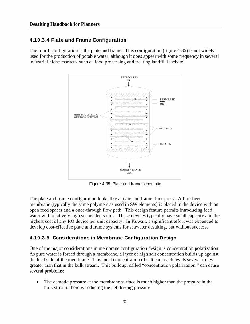
Desalting Handbook for Planners
92
4.10.3.4 Plate and Frame Configuration
The fourth configuration is the plate and frame. This configuration (figure 4-35) is not widely used for the production of potable water, although it does appear with some frequency in several industrial niche markets, such as food processing and treating landfill leachate.
Figure 4-35 Plate and frame schematic
The plate and frame configuration looks like a plate and frame filter press. A flat sheet membrane (typically the same polymers as used in SW elements) is placed in the device with an open feed spacer and a once-through flow path. This design feature permits introducing feed water with relatively high suspended solids. These devices typically have small capacity and the highest cost of any RO device per unit capacity. In Kuwait, a significant effort was expended to develop cost-effective plate and frame systems for seawater desalting, but without success.
4.10.3.5 Considerations in Membrane Configuration Design
One of the major considerations in membrane configuration design is concentration polarization. As pure water is forced through a membrane, a layer of high salt concentration builds up against the feed side of the membrane. This local concentration of salt can reach levels several times greater than that in the bulk stream. This buildup, called “concentration polarization,” can cause several problems:
• The osmotic pressure at the membrane surface is much higher than the pressure in the bulk stream, thereby reducing the net driving pressure
FEEDWATER
PERMEATE
CONCENTRATE
IN
OUT
OUT
MEMBRANE ENVELOPEWITH POROUS SUPPORT
O-RING SEALS
TIE RODS

Chapter 4: Desalting Processes
93
• Salt transport through the membrane increases (because of the increased salt concentration gradient), resulting in product quality deterioration
• Compounds like calcium sulfate and calcium carbonate are more concentrated and more likely to precipitate
One effective way to combat concentration polarization is to maintain adequate feed/concentrate velocities through the unit. This can be done by carefully adhering to the membrane manufacturer’s recommendations for minimum flow rates and maximum pressure drops during the process design phase.
4.10.4 Power Consumption
The electrical energy consumed by the RO process is primarily for pumping. In the last 10 years, the net driving pressure (NDP) required for permeation has been significantly reduced, and the in-process electrical energy needs have declined.
The NDP required for any given membrane application in RO and NF is a function of both the osmotic pressure change and hydraulic resistance, and can be calculated from the following expression:
)Pnet = PF – ()P/2 + Πave + Pp - Πp)
where:
)Pnet = net driving pressure PF = membrane feed pressure )P = pressure drop across the feed/concentrate side Πave = average osmotic pressure, feed/concentrate side Pp = product water back pressure Πp = product water osmotic pressure
An approximation of this equation is:
)P = PF – PC
PC = concentrate pressure
Product water osmotic pressure, Πp, is generally ignored, since it is small compared to the other terms. Product water back pressure, PP, is becoming more significant as the NDP for commercial brackish water membranes declines. In a typical brackish water application, PP can range from 3 to 10 m (approximately 10 to 30 ft) of water column, as the water is directed to either a ground storage tank or a degassifier.

Desalting Handbook for Planners
94
The NDP required is influenced by the concentration factor in the process and, thus, the water recovery. Recovery (R) is the term used to describe the efficiency of the process in terms of yield, and is usually measured as the fraction of feed water recovered as permeate. That is:
R = (QP/QF ) 100 percent
Temperature also impacts energy consumption in RO feed pumps, since temperature affects flux, and flux impacts NDP. Flux increases as NDP increases.
High efficiency of both the motor and the pump should be the primary guideline in selecting feed pumps. Variable frequency drives now are commonplace in brackish water RO plants. These frequency drives should be selected on the same basis. Typical feed pump energy requirements for brackish water RO plants range from 0.5 to 2 kWh/m3 (1.9 to 7.6 kWh/kgal). Requirements for seawater RO plants are now typically less than 3 kWh/m3 (11.4 kWh/kgal) with the use of energy recovery devices.
Some examples of power requirements are shown in table 4-9.
Table 4-9.—Typical RO feed pump power consumption
Location
Feed TDS
(mg/l)
Recovery (percent)
Temperature
(oC)
Feed pressure
(bars)
Feed pump power
(kWh/m3)
Feed pump
type
Jupiter, FL1 (Phase I) 5,000 75 21 24 1.125 VT
Jupiter, FL2 (Phase II) 5,000 75 21 614.4/17.2 0.650 VT
Cape Coral, FL Plant 2 1,300 85 28 12.5 0.454 VT
Kill Devil Hills, NC3 32,300 75 20 18.2 0.828 VT
Santa Barbara, CA SSW 40 10-15 60-65 3.5-4.0 HMS
Key West, FL4 SWW 30 20-28 55-60 4.0-4.5 VT
Arlington, CA4 1,200 77 21 14.5 0.515 VT
Marco Island, FL5 ~10,000 75 21 623.1/27.2 1.111 VT
1 Hydranautics CPA-2 2 Hydranautics ESPA with interstage boost 3 Feed water now ~ 4,000 mg/l TDS 4 With energy recovery, reverse running turbine between pump and motor 5 Uses hydraulic TurbochargerTM as interstage boost 6 First and boosted second stage pressures Note: VT = vertical turbine, can type HMS = horizontal, multi-stage with energy recovery turbine

Chapter 4: Desalting Processes
95
Energy recovery has become fairly commonplace in the specification of seawater RO systems. There are four basic types:
• Pelton Wheel
• Work exchanger
• Pressure exchanger
• Hydraulic Turbocharger
Figure 4-36 shows photos of three of these energy recovery devices in operation. In general, the energy recovered is between 25 and 35 percent of the input energy for seawater RO (Oklejas, et al., 1996).
The large seawater plants being built today in Spain, Trinidad, and at Tampa Bay, Florida all use Pelton Wheel energy recovery devices. In these sizes, 454 m3/hr (2,000 gpm) and larger, recovery efficiency is high, above 80 percent in most cases. The pressure exchanger is currently used for smaller systems and has even higher efficiency (above 90 percent). Turbocharger efficiency is currently between 60 and 70 percent and is also size limited, with the largest unit currently in production sized for 409 m3/hr (1,800 gpm).
Until the introduction of “ultra” low-pressure brackish water membranes, there was little incentive to include energy recovery devices in the process design, except where the TDS was high and recovery was low. However, given the characteristics of current low-pressure membranes, reduced feed pressure with interstage boost using energy recovery devices has been successfully employed at some locations (Duranceau et al., 1999; Nemeth and Tomkins, 2001).
4.10.5 RO Process Variables
Recovery is the most important process variable, and the one the other variables largely depend on. Recovery controls the concentration factor, CF:
CF = 1/(1-R)
where:
R = recovery expressed as a fraction
Figure 4-37 shows the concentration factor as a function of recovery, assuming a perfect membrane. Using these values will result in a slightly conservative design.

Desalting Handbook for Planners
96
Figure 4-36 Three types of energy recovery devices in use today
Small Pelton Wheel, serving two small SWRO units
Hydraulic Turbocharger Heat Transfer Chamber (HTC®)
Work exchanger

Chapter 4: Desalting Processes
97
Figure 4-37 Solute concentration factor as a function of recovery
Recovery is limited by water chemistry for brackish systems and pressure requirements for seawater systems. Other process variables that must be considered are:
• Flux.—The value of flux will determine the membrane area to be used and the feed pressure requirement. Flux also impacts the rate of fouling.
• Feed rate per vessel.—This rate will also impact the feed pressure requirement by impacting the system pressure drop. It establishes cross-flow velocity and affects concentration polarization.
• Minimum concentrate flows.—Flow across the membrane surface is an important consideration in controlling concentration polarization.
• Product water quality.—Quality can be impacted by the selection of membrane type and flux.
• Temperature.—Temperature is very important in the process design stage, since temperature has a significant impact on flux and, therefore, the capital and operating costs. While ground water temperatures are relatively constant, seawater temperature from open intakes can vary widely.
0.00
10.00
20.00
30.00
40.00
50.00
0% 10% 20% 30% 40% 50% 60% 70% 80% 90% 100%
Recovery, Permeate as % of Feed
Con
cent
ratio
n Fa
ctor
Desalting Handbook for Planners
98
4.10.6 RO and NF Peripheral Equipment
In addition to the membrane assemblies themselves, other process equipment includes:
• Fine filtration.—This usually involves the use of cartridge filters of 5-10 microns nominal retention. Figure 4-38 shows horizontal cartridge filters. These filters are not designed to perform routine filtration, but to prevent unusual changes in the quality of the feed water source (upsets) from damaging either the feed pump or the membranes. Sometimes, these cartridge filters are located downstream of the feed pumps. In such cases, a fine mesh strainer would be included to protect the pump.
• Scale control systems.—Most RO systems require adding a scale inhibitor and, sometimes, acid for scale control in the membrane array, since at least one constituent of the feed water will probably be supersaturated in the concentrate. Systems for storing and introducing these chemicals include bulk and day storage tanks, metering pumps, calibration tubes, and monitoring and control systems. Proper safety equipment must also be provided. Figure 4-39 shows a typical chemical feed system.
• Cleaning system.—It is good practice to include a cleaning system in the requirements for a commercially sized RO system. A typical cleaning system consists of one or two tanks, a recirculation pump, a fine filtration device, and monitoring instrumentation. Figure 4-40 shows a cleaning system.
Figure 4-38 Horizontal cartridge filters in Jupiter, Florida

Chapter 4: Desalting Processes
99
Figure 4-39 Typical chemical feed system
Figure 4-40 Cleaning system, North Hatteras plant, Dare County, North Carolina
Acid feed system at Jupiter, Florida, showing metering pumps, day tank, and calibration columns. This acid system serves two separate RO plants, each one processing 22,700 m3/d (6.0 mgd).

Desalting Handbook for Planners
100
4.10.7 RO Plant Layout
Figure 4-41 shows a simple flow diagram of an RO system. Incoming feed water is given the required pretreatment, the RO feed pump raises pressure in the feed water, and the pressurized water then enters the membrane assembly. The arrangement of vessels in parallel and series groups determines the recovery and capacity.
Figure 4-41 Simplified RO process flow diagram
Spiral wound membranes are loaded into pressure vessels. These vessels are made from either fiberglass-reinforced plastic or stainless steel. The pressure vessels can hold from one to eight standard 1,016-cm (40-inch) elements. Typically, for large brackish water and NF systems for potable water production and wastewater reclamation, vessels are selected to hold six or seven standard 203-cm (8-inch) diameter by 1,016-cm (40-inch) long membrane elements. For seawater systems, it is now more common to find systems using seven-element-long vessels in one or two stages, as shown in figure 4-42. A seven-element vessel system requires a space about 7.62 m long (25 ft). In addition, at least 1.2 m (4 ft) is required at each end for vessel handling, for a total length requirement of 10-10.7 m (33-35 ft). The width depends on the capacity of the unit and the type of feed water. Review of actual installations indicates that an average plant area of 0.022-0.029 m2 per m3 (900-1,200 ft2 per million gallons) of output. Table 4-10 gives guidelines for selecting vessel length based on recovery.

Chapter 4: Desalting Processes
101
Figure 4-42 Typical arrangements for staging
Table 4-10.—Typical recoveries for various vessel lengths
No. of elements
per vessel
Maximum recovery per stage standard pressure
(percent)
Maximum recovery per stage low pressure
(percent)
4 40 35
5 50 45
6 55 50
7 65 60
8 75 N/A
• The membrane product tubes of elements in a vessel are connected together with O-ring-sealed interconnectors. Vessels are then grouped in parallel to form stages, and the stages are arranged in series to maintain adequate cross flow and minimum concentrate flow.
• The concentrate control valve maintains the back pressure on the membrane system so that the NDP requirements of the stages can be met. In some ultra-low pressure applications, product water back pressure on the first stage or interstage boost pumping may be required to control flux in the lead membranes and to prevent premature fouling.
product
concentrate
concentrate
product
product
concentrate
(Taper = 2:1 typical)
(Taper = 3:2:1 typical)
a) Single stage ~ maximum recovery 55 percent
b) Two stage ~ maximum recovery 80 percent
c) Three stage ~ maximum recovery 90 percent

Desalting Handbook for Planners
102
4.10.8 Membrane Life
The useful life of RO and NF elements is usually a function of the membrane material and the application. For cellulose membranes, the lifespan most commonly used in planning is 3 to 5 years. However, there have been examples of much longer life, particularly when RO elements were used to treat anaerobic ground water.
Noncellulosic membranes can operate over a much wider range of pH. Most, however, have a limited resistance to chlorine and other strong oxidants. Typically, for planning purposes, the lifespan for noncellulosic elements is estimated at 5 to 7 years. However, some systems have spiral wound elements that are 10 years old and still operational, while it has been reported that in some HFF systems, permeator performance has been maintained for over 15 years.
4.11 Comparing RO and NF with Other Desalting Processes
The RO process is now in daily operation worldwide in applications ranging from producing ultrapure water to converting seawater to drinking water. Sizes range from a few m3/d to the massive Yuma Desalting Plant, at 272,500 m3/d (72 mgd). The largest operating membrane plant in the U.S. is an NF plant in Boca Raton, Florida.
RO for brackish water can remove organics and microorganisms from the feed water. NDP requirements have been greatly reduced in recent years, resulting in lower operating costs. Conversely, today’s RO membranes have higher salt rejection characteristics, permitting higher blend ratios. Suitably treated raw water is sometimes blended with product water to reduce RO equipment size and to remineralize low TDS permeate. Specialized membranes, such as NF, and ultra-low pressure have widened the application spectrum.
Generally, RO has lower capital and operating costs than distillation processes. RO feed pumps may be driven by steam turbines, allowing coupling to steam producers such as cogeneration facilities. Materials selection is important, but not as critical as it would be for the high temperature thermal processes. Pretreatment is especially critical for RO, particularly because pretreatment adds to the capital and operating costs of the process.
References
Chapman-Wilbert, M. et al., “The Desalting and Water Treatment Membrane Manual: A Guide to Membranes for Municipal Water Treatment,” (2nd edition). Water Treatment Technology Program Report No. 29, Bureau of Reclamation, Denver, Colorado, 1998.

Chapter 4: Desalting Processes
103
Duranceau, S.J., et al., “Interstage Turbines as Self-Regulating Pressure Control Valves in a Desalting Facility,” Proceedings of the American Water Works Association Membrane Technology Conference, Long Beach, California, February 1999.
Eisenberg, T.N., and E.T. Middlebrooks, “Reverse Osmosis Treatment of Drinking Water,” Butterworths, 1986.
Elyanow, D, et al., “Desalination of Brackish Ground Water for a Prairie Community Using Electrodialysis Reversal,” Proceedings of the Twelfth International Symposium on Desalination and Water Re-Use, Malta, April 15-18, 1991.
Fluid Systems, “Seawater Reverse Osmosis Guidelines,” July 1997.
Mallevialle, J., et al., “Water Treatment Membrane Processes,” McGraw-Hill, 1996.
Meller, F., ed., “Electrodialysis and Electrodialysis Reversal Technology,” Ionics, Inc, 1984.
Nemeth, J.E., and B. Tomkins, “Energy Recovery Devices: Comparison and Case Studies,” Proceedings of the American Water Works Association Membrane Technology Conference, San Antonio, Texas, March 2001.
Oklejas, E., et al., “Improvements in the Economics of Reverse Osmosis through Advanced Pumping and Energy Recovery Technology,” Proceedings of the American Desalting Association, Monterey, California, August 4-8, 1996.
Speigler, K.S., and A.D.K. Laird, “Principles of Desalination, 2nd edition,” Academic Press, 1980.
Speigler, K.S., and Y.M. El-Sayed, “A Desalination Primer,” Balaban Desalination Publications, 1994.
Wade, N.M., “Technical and Economic Evaluation of Distillation and Reverse Osmosis Desalination Processes,” Desalination 93, 1993.
Wangnick, K., “2000 IDA Worldwide Desalting Plants Inventory, Report No. 16,” International Desalination Association, May 2000.
Wangnick, K., “2002 IDA Worldwide Desalting Plants Inventory, Report No. 17,” International Desalination Association, May 2002.
Watson, I.C., “Membrane System Applications and Economics,” Proceedings of the American Water Works Association Conference, Orlando, Florida, 1988.
Werner, T.E., and A.T.M.Gottburg, “5 Billion Gallons Later – Operating Experience at the City of Suffolk EDR Plant,” Proceedings of the American Desalting Association, Williamsburg, Virginia, August 2-6, 1998.


Chapter 5: Pretreatment
105
Chapter 5: Pretreatment
5.1 Introduction
Some pretreatment of the feed water for a desalting plant is generally always required. Pretreatment ensures that constituents that are present in the raw water supply do not result in a loss of performance or a reduction in the output of the facility during normal operation of the plant.
Each desalting technology has different requirements for the quality and condition of water entering the process. For distillation processes, the concerns are:
• Scaling of the heat exchanger tube surfaces • Corrosion of the plant components • Erosion by suspended solids • Effect of other constituents
For membrane processes, the major concerns are:
• Membrane fouling and scaling • Suspended solids plugging • Biological fouling or attack • Membrane degradation by oxidation or other means
5.2 Distillation Processes
5.2.1 Scaling in Distillation Processes
In distillation processes, calcium sulfate, CaSO4, magnesium hydroxide, Mg(OH)2, and calcium carbonate, CaCO3, in the water can cause scaling on the tube surfaces. Scales form as these compounds precipitate out of the feed water.
5.2.1.1 Calcium Sulfate Scaling
Removing either the calcium or the sulfate from the water supply is one way to prevent calcium sulfate scaling in the pretreatment process. This approach, however, is generally not cost effective. The traditional means of controlling calcium sulfate scaling is to operate the plant at lower temperatures or use antiscalants. Nanofiltration (NF) pretreatment is another technique that is sometimes used to reduce the potential for calcium sulfate scaling for both distillation and reverse osmosis (RO) systems (Hassan, 1999).

Desalting Handbook for Planners
106
Calcium sulfate has a reverse solubility curve. This means that the solubility decreases with an increase in temperature. In other words, the higher the temperature, the greater the rate of precipitation and the greater the potential for scale formation.
5.2.1.2 Calcium Carbonate and Magnesium Hydroxide Scaling
These chemical compounds predominate (or form) at lower temperatures. Scale formation can be prevented by removing the bicarbonate ions. The bicarbonate ion, HCO3
-, is responsible for calcium carbonate and magnesium hydroxide scale formation. Therefore, eliminating this ion prevents scale from these two compounds. The bicarbonate ion is readily removed by treating the feed water with acid. Sulfuric acid, H2SO4, reacts with the bicarbonate ion to produce an unstable carbonic acid, H2CO3, which, in turn, decomposes to form water and carbon dioxide gas. In order to bring this reaction to completion, the carbon dioxide gas is stripped from the seawater feed water in a decarbonator. Alternatively, additives can be used as discussed in chapter 4.
5.2.2 Corrosion in Distillation Processes
Corrosion within the evaporator depends on:
• Amount of gases entering unit • Temperature of operation • Concentration of chloride ion • pH
Pretreating the feed water helps influence these variables to prevent corrosion.
Amount of gases.—The amount of corrosive gases entering the evaporator can be minimized by using a decarbonator and deaerator. The decarbonator will remove carbon dioxide, while the deaerator removes oxygen. Sodium bisulfite, or a similar oxygen scavenger, is then added to the make-up stream as it exits the deaerator to ensure all oxygen has been removed.
Temperature of operation.—The maximum temperature of operation will be determined by the process type and chemicals used for pretreatment. Polyphosphate is effective for temperatures up to 90.6 oC (195 oF). For operation at higher temperatures, acid or carbolic-type polymers are required. These pretreatment systems do not prevent corrosion within the unit.
Concentration of the chloride ion.—Corrosion due to the concentration of chloride cannot be eliminated by pretreatment. To prevent corrosion from chloride ions, construction materials that resist this corrosion are required. For example, SS316L cannot be used in applications where the chlorine content exceeds 1,000 parts per million (ppm).
pH.—By adding acid, the pH of the feed water can be lowered enough to lower the concentrate of the bicarbonate ion. This is accomplished by lowering the pH to a value of 4.2 to 4.5. However, if the carbon dioxide produced by adding acid is allowed to enter the evaporator, it

Chapter 5: Pretreatment
107
could result in severe corrosion. Carbon dioxide gas is removed in a decarbonator before the feed water enters the evaporator. This step results in further elevating the pH to between 5.5 and 6.0.
5.2.3 Erosion by Suspended Solids in Distillation Processes
Sand is the only suspended solid of concern for distillation processes. If sand is allowed to enter the evaporator, the tubing surfaces will erode. Such processes will lead to early replacement of the tube bundles, with consequent increase in the cost of water. In addition to causing tube erosion, sand can plug spray nozzles, which can result in frequent unit shutdowns for cleaning.
5.2.4 Impact of Other Constituents
Hydrogen sulfide.—Some feed waters (particularly ground water) contain hydrogen sulfide, H2S, which must be removed from the feed water before it enters the unit. Hydrogen sulfide reacts with materials such as copper and nickel, which are typically used for heat transfer surfaces in distillation processes. The sulfides react with the copper/nickel to reduce the heat transfer and ultimately lead to tube failure.
Oil.— This contaminant must also be removed in the pretreatment system. If oil is not removed, it will foul the evaporator tube surfaces, resulting in a loss of heat transfer.
Marine growth.—Marine growth can occur in the feed water intake and supply line. This is generally taken care of by adding chlorine early in the feed water supply. Chlorine is added at low dose rates of 0.5 milligram per liter (mg/l) or less. Periodic shock treatment at dose ratios as high as 5.0 mg/l may also be required.
Heavy metals.—If the evaporator is constructed with aluminum parts, metals such as copper, nickel, and mercury must be removed from the feed water before it enters the evaporator. This is accomplished using an “ion trap.” The ion trap is simply a vessel containing small “chips” of the same aluminum material used for the fabrication of the unit. The metals react with this sacrificial aluminum and are removed in the trap.
Figures 5-1 and 5-2 show typical pretreatment schematics for operation at low temperature with polyphosphate addition or high temperature with acid addition.

Desalting Handbook for Planners
108
Figure 5-1 Pretreatment schematic, low temperature design ( T = 90 oC)
Figure 5-2 Pretreatment schematic, high temperature design ( T = 110 oC)
5.3 Membrane Processes
Pretreatment is essential for proper operation of RO and electrodialysis reversal (EDR) equipment and can add substantially to the project’s capital and operating costs. Three main types of membrane scaling and fouling are considered in this section:
Pre-chlorination
Oil/Sand Removal(if required)
Acid Treatment
Ion Trap
To EvaporatorOxygen Scavenger
Intake Chamber
Feed PumpDe-Aerator
To Air Ejector
(if required)
Travelling Screen& Trash Rack
Decarbonator
Pre-chlorination
Oil/Sand Removal(if required)
Polyphosphate treatment
Ion Trap
To EvaporatorOxygen Scavenger
Intake Chamber
Feed PumpDe-Aerator
To Air Ejector
(if required)
Travelling Screen& Trash Rack

Chapter 5: Pretreatment
109
• Scaling: mainly alkaline and nonalkaline scale, such as calcium sulfate
• Fouling by metal oxides: mainly iron or manganese, but oxidized hydrogen sulfide is also a concern
• Fouling by suspended solids, colloids, and/or biological growth
Table 5-1 lists the general pretreatment requirements for RO and EDR membrane systems. Pretreatment goals are to control:
• Biological activity and fouling • Metal oxide fouling • Mineral scale • Silica precipitation • Colloidal fouling • Particulate fouling
Table 5-1 Pretreated water quality requirements for membrane processes
Spiral CA Spiral PA EDR
Suspended matter
a) Turbidity, NTU <1.0 <1.0 <5
b) SDI <4.0 <4 <15
Ionic content
a) Iron, mg/l (ferrous) <2.0 <2.0 <0.1
b) Manganese, mg/l <0.5 <0.5 <0.1
c) Strontium, in conc percent saturation 2,000 percent 3,000 percent 4,000 percent
d) Barium, in conc percent saturation 5,000 percent 5,000 percent 7,000 percent
e) Silica, mg/l (w/o inhibitor) in concentrate <160 <160 <saturation in feed
Chemical Additives
a) Residual Chlorine, ppm <1.0 ND ND
b) Scale Inhibitor, mg/l in concentrate 12-18 12-18 As required
c) Acidification, pH 5.5-6.0 4-10 As required
Temperature, saturation, solubility
Maximum feed temperature oC 40 45 43
Maximum LSI with scale inhibitor Note +2.4-+2.8 2.1
Solubility product (CaSO4) with scale inhibitor, percent saturation
150 percent 150 percent 650 percent
NA = Not applicable ND = Nondetectable SDI = Silt Density Index NTU = Nephelometric turbidity units Type of membrane: PA = Polyamide CA = Cellulose acetate EDR = Electrodialysis reversal
Note: CA membranes require acidification to pH 5.5 to 6.0 to reduce the rate of hydrolysis. Therefore, the Langelier Saturation Index of the exiting concentrate tends to be low enough that scale inhibitor for calcium carbonate is not necessary.
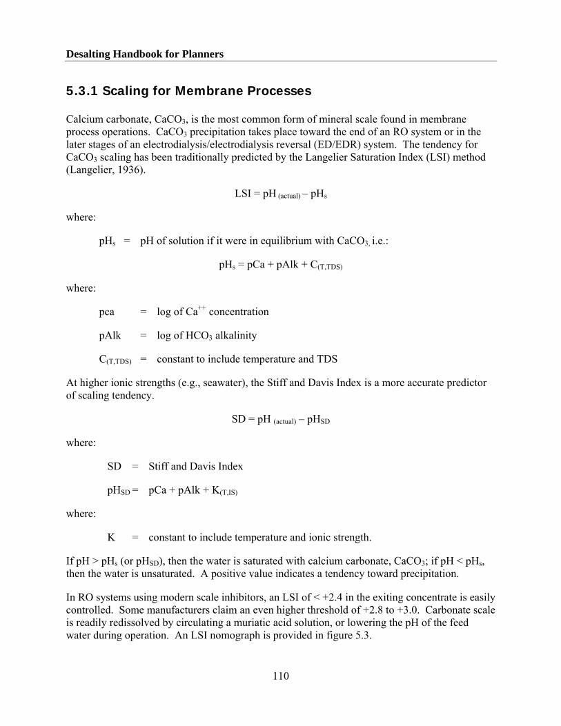
Desalting Handbook for Planners
110
5.3.1 Scaling for Membrane Processes
Calcium carbonate, CaCO3, is the most common form of mineral scale found in membrane process operations. CaCO3 precipitation takes place toward the end of an RO system or in the later stages of an electrodialysis/electrodialysis reversal (ED/EDR) system. The tendency for CaCO3 scaling has been traditionally predicted by the Langelier Saturation Index (LSI) method (Langelier, 1936).
LSI = pH (actual) – pHs
where:
pHs = pH of solution if it were in equilibrium with CaCO3, i.e.:
pHs = pCa + pAlk + C(T,TDS)
where:
pca = log of Ca++ concentration
pAlk = log of HCO3 alkalinity
C(T,TDS) = constant to include temperature and TDS
At higher ionic strengths (e.g., seawater), the Stiff and Davis Index is a more accurate predictor of scaling tendency.
SD = pH (actual) – pHSD
where:
SD = Stiff and Davis Index
pHSD = pCa + pAlk + K(T,IS)
where:
K = constant to include temperature and ionic strength.
If pH > pHs (or pHSD), then the water is saturated with calcium carbonate, CaCO3; if pH < pHs, then the water is unsaturated. A positive value indicates a tendency toward precipitation.
In RO systems using modern scale inhibitors, an LSI of < +2.4 in the exiting concentrate is easily controlled. Some manufacturers claim an even higher threshold of +2.8 to +3.0. Carbonate scale is readily redissolved by circulating a muriatic acid solution, or lowering the pH of the feed water during operation. An LSI nomograph is provided in figure 5.3.

Chapter 5: Pretreatment
111
Figure 5-3 Langelier Saturation Index nomograph
For EDR plants, CaCO3 scale is rarely a problem. If it occurs, cleaning with hydrochloric acid and adding a small amount of scale inhibitor to the concentrate recirculation system can be used to reduce and eliminate the problem.
Sulfate scales of calcium, strontium, and barium are also important factors in RO and ED/EDR operations. Before synthetic scale inhibitors were available, the recommended procedure was to keep the calcium sulfate saturation to less than 100 percent. Nowadays, a value of twice saturation is controllable, provided a reliable, monitored system for scale inhibitor addition in the right amount is included in the design. Barium and strontium sulfates, BaSO4 and SrSO4, are extremely insoluble but, fortunately, they tend to form very slowly and, thus, are controllable at high levels of supersaturation. Commonly used values for BaSO4 are 30 to 70 times saturation. In EDR systems, a much higher level of supersaturation is possible in some cases.
In predicting the solubility limits of sulfates, it is important to remember two points:
1. Modern RO membranes reject divalent ions very well. Therefore it is reasonable to assume a zero percent salt passage when calculating the concentration factor, CF.
2. Compounds are more soluble in the concentrate than in the feed water. The solubility product constant, KSP1, of each compound increases with ionic strength.
3as mg/l CaCO++Ca
3mg/l CaCO3HCO as
3pHCO
o
o
o
o
o
o o
oo
ooo
o o
o o
oo
43.3 C (110 F)
37.8 C (100 F)
32.2 C (90 F)
26.7 C (80 F)
21.1 C (70 F)15.6 C (60 F)
10 C (50 F)
4.4 C (40 F)
0 C (32 F)
2.9
2.8
2.7
2.6
2.5
2.4
2.3
2.2
2.1
2.0
1.9
1.8
1.7
50001000500200100502010521
3 as CaCO= 774.8 mg/l
LSI = +1.91bpH
= 6.28SpHC = 2.37 = 1.81
3pHCO
pCa = 2.10 (use 5000 mg.l)TDS = 7853.6 mg/l
_3HCO
3 CaCO = 800 mg/l as
++CapH = 7.6
oTemp = 20 C
Example
1.0
2.0
3.0
4.0
5.0
pHC
O
and
pCa
Scal
e3
= 8.19
mg/l
pCa
TDS Constant "C"
"C"
Scal
e

Desalting Handbook for Planners
112
As a rule of thumb, scale inhibitor dosages for RO systems are calculated as concentrations in the concentrate of 12-18 mg/l. This value is then converted to a feed water dosage using the CF for the design recovery, and assuming 0 percent salt passage. In ED/EDR systems, the scale inhibitor is added to the recirculating concentrate stream, while an equivalent amount is “wasted” in the concentrate blowdown.
SI(f) = SI(c) / CF
where:
SI(f) = scale inhibitor concentration in the feed water, mg/l
SI(c) = scale inhibitor concentration in the exiting concentrate, mg/l
CF = the concentration factor at the operating recovery
Table 5-2 shows the characteristics of some commercially available scale inhibitors. It is important to remember that any product added to drinking water systems must have National Sanitation Foundation (NSF) certification under NSF Standard 60, Drinking Water Additives.
Although temperature is seldom an influence in membrane scaling control strategies, it is important to remember that CaCO3 has a somewhat inverted solubility curve after about 35 oC. In some U.S. locations (e.g., Laredo, Texas; and Mount Pleasant and Hilton Head, South Carolina), the feed water temperature for RO is >35 oC (95 oF).
In addition to calcium carbonate and sulfate scales, the potential exists, at least theoretically, for other soluble compounds (e.g., calcium fluoride and calcium phosphate) to cause problems in membrane desalting applications. These can usually be controlled by using the same techniques that work to control the more common scaling salts.
5.3.2 Metal Oxide Fouling in Membrane Processes
The oxides of several metals are extremely insoluble. Oxides of ferric iron, Fe3+, and manganese, Mn3+, are of principal concern in membrane plants. RO is generally more tolerant of feed waters containing iron and manganese than EDR, since the electrochemical nature of the EDR process results in releasing oxidants in the EDR stack. However, the reversal process has increased the ED process’ tolerance to these metals in the feed water.
In RO applications, it is recommended that the amount of iron and manganese in the feed water be limited to no more than 2.0 mg/l of iron and no more than 0.5 mg/l of manganese. Higher concentrations may cause problems of co-precipitation with other constituents, such as silica. This is particularly important for RO drinking water systems, since the concentrations of iron and manganese are limited by the secondary drinking water standards.

Chapter 5: Pretreatment
113
Table 5-2. —Typical commercial scale inhibitors
Active ingredient Trade name
Designation Type % wt
Specific gravity
pH
Appearance
Application
PC-191 Blend NA 1.36 10.5 Pale yellow liquid General
PC-391 Blend NA 1.10 11.0 Clear, colorless liquid
Small flow systems/ recycle systems
PermaTreat™1
PC-510 Blend NA 1.22 9.7 Amber liquid Silica control
100 NA 35 1.17 3.5 Pale yellow liquid Inorganic scale Flocon™
260 NA 35 1.16 <2.0 Pale yellow liquid Dispersant
600 Blend 35 1.2 3.0-4.0 Water white to amber
Inorganic scale control
820 Blend 37 1.2 4.3-5.3 Water white to amber
Dispersant and metal ion stabilizer
1025 Blend 36.5 1.15 2.5-5.3 Water white to
amber
Inorganic scale control and dispersant
Aquafeed Antiscalent ™2
1405 Blend 29 1.1 4.1-5.1 Water white to amber liquid
Silica and silicate control
MDC 120 Poly-acrylic acid NA 1.05-1.15 3.56 Pale to amber liquid General
MDC 150 Poly-electrolyte blend
NA 1.1-1.2 2.56 Pale to dark amber liquid Inorganic scales
Hypersperse™3
MSI310
Poly-electrolyte polymer blend
NA 1.05-1.15 4.8-5.5 Pale to amber liquid Silica
0100 Blend NA 1.03-1.09 1-2 Colorless liquid Inorganic scales and gels
1100 Blend NA 1.04-1.13 2.6 Colorless liquid Inorganic scales
NSF Blend NA 1.35-1.55 5.3 Light brown liquid Inorganic scales
Silica Blend NA 1.03-1.09 1-2 Colorless liquid Reactive silica
2000 Blend NA 1.03-1.13 10.0 Light brown liquid Inorganic scales
Pretreat Plus™4
Y2K Blend NA 1.04-1.14 1-2 Colorless liquid Inorganic scales and gels
0200 Blend NA 1.14 1.5 Pale yellow liquid Inorganic scales and gels
0300 Blend NA 1.07 2.0 Amber liquid Inorganic scales and gels
0400 Concentrate Blend NA 1.3 7.0 Pale yellow liquid Inorganic scales and
gels
ProTec RO Blend NA 1.03 5.2 Straw colored liquid Colloidal silica and silt
ProTec RO-B Blend NA 1.04 7.5 Colorless liquid Microbial colloids
ProTec RO-C Blend NA 1.07 8.0 Yellow liquid Colloidal organics and sulfur
ProTec RO™5
ProTec RO-D Blend NA 1.02 6.0 Colorless to light yellow liquid Mixed colloidals
1 Information from Nalco, Inc., 2002. PermaTreat is a registered trademark of Ondeo Nalco, Ltd. 2 Information from Noveon, Inc., 2002. 3 Information from GE Betz, Inc., 2002. 4 PreTreat Plus are antiscalants. Information from King Lee Technologies, 2002. 5 ProTec RO are antifoulants. Information from King Lee Technologies, 2002.

Desalting Handbook for Planners
114
For EDR, the iron concentration should be limited to 0.3 mg/l, and manganese to 0.10 mg/l. Relatively high levels of iron may also influence the effectiveness of scale inhibitors, possibly leading to premature precipitation of scale-forming compounds.
When designing the membrane plant, the feed water system must be kept anaerobic, so that iron and manganese remain in the soluble divalent or “-ous” state, rather than be oxidized to the insoluble trivalent, or “-ic” state. This condition assumes no other design influences.
5.3.3 Biological Fouling in Membrane Processes
Biofouling is a significant concern resulting in a loss of flux and an appreciable increase in the hydraulic pressure drop through the feed concentrate spacer. Although biofilm formation is generally a precursor to biofouling, biofilm can exist on the membrane surface in the absence of detectable biofouling (Costerton et al., 1985).
Even in clear, brackish well waters, the potential for biofouling can exist. In the early days of RO development, cellulose acetate membranes were susceptible to attack from a variety of bacteria. Holes appeared in the membrane surface, resulting in a rapid increase in both flux and salt passage. More typical, however, was the loss of flux due to biofouling over days or weeks, resulting in a change in salt passage and a significant increase in power requirements. Chlorine disinfection can be used to control biofouling in situations where it can be shown that chlorine in small dosages does not harm the membranes.
A list of the mechanisms that may lead to biofouling is incorporated into table 5-3. A diagram of the adhesion to the membrane surface is shown in figure 5-4.
With the advent of polyamide and other noncellulosic membrane materials, the use of chlorine, or other strong oxidants within the membrane system becomes unacceptable, due to the potential for membrane degradation. However, these membrane materials typically are resistant to biological attack. The challenge then is to prevent or control the formation of biofilm on the membrane surface (Costerton et al., 1985).
A significant body of work exists, describing efforts to develop techniques for preventing the adhesion of biofilm in a dynamic, operating environment. Evaluating disinfection strategies and increasing focus on mechanical and process design issues are alternative approaches. Biofilm adhesion interference has been demonstrated, but very few techniques are available that do not cause significant and permanent loss of membrane performance. Feed water disinfection, usually with chlorine followed by dechlorination, likewise has had mixed results. A significant amount of work with CA membranes has been undertaken by the Bureau of Reclamation in conjunction with maintenance of CA membranes at Yuma, Arizona (Henthorne and Lichtwardt, 1996).

Chapter 5: Pretreatment
115
Table 5-3 Principal events in membrane biofouling processes Event Time To onset1 Description/explanation
Primary organic film
Seconds/minutes Typically referred to as the conditioning film; defined as the rapid adsorption of dissolved organic macromolecules and inorganic substances at the membrane/liquid interface.
Primary cell adhesion
Seconds/minutes Refers to pioneer bacterial attachment; depends on nature of cell surface, membrane type, feed water chemistry, and system hydrodynamics; provides major contribution to early biofilm accumulation.
Cellular detachment
Seconds/minutes Influences biofilm accumulation rate; detachment is sometimes enhanced by micro-biocidal agents, dispersants, etc.
Cell growth/ multiplication
Minutes/hours Occurs at expense of soluble and sorbed feed water nutrients; may provide greatest contribution to biofilm formation where biocides are not present.
Biopolymer (EPS) synthesis
Minutes/hours Provides for greater biofilm structural integrity; acts as a reactive transport barrier to chemical biocides; promotes nutrient concentration/storage.
Particle/colloid entrainment
Seconds/minutes Secondary effect where suspended particles and colloidal material are passively entrained in the biopolymer matrix or within biofilm void spaces.
Secondary cell adhesion
Days/weeks Commences after primary biofilm formation by pioneer cells; probably strongly influenced by surface properties and physiology of primary biofilm and leads to greater species diversity.
Biofilm sloughing Days/weeks Refers to cell and biomass detachment; occurs in response to changes in hydrodynamic shear or turbulence forces, or introduction of biocides, dispersants, etc.
Biofilm senescence
Weeks/months Refers to accelerated cell die-off in old biofilms; cell death is in equilibrium with biofilm growth in continuous flow systems; may result in release of soluble nutrients via cell lysis.
1 Time after a membrane is placed into operation.
Prevention and/or control of biofouling are typically site specific. Some process and design steps to assist in biofouling control:
• Thorough source water investigation • Good process design • Good mechanical design • Thorough understanding of water quality • Good operator training • Selection of effective disinfectants and biocides • Routine system disinfection • Maintain anaerobic conditions throughout process

Desalting Handbook for Planners
116
Figure 5-4 How a bacterium sticks to the membrane surface
5.3.4 Suspended Solids in Membrane Processes
While generally not a consideration with properly constructed and maintained ground water systems, suspended solids can be a major concern when treating surface water or reclaiming wastewater.
Suspended solids in feed water for membrane processes can consist of inorganic materials, such as clays, insoluble metal oxides, and organic substances such as colloidal color.
Conventional water treatment practices (shown in table 5-5) can be used to reduce or remove the suspended solids from the feed water, with varying degrees of success. Early examples of this are the pretreatment system for Water Factory 21, operated by the Orange County Water District in Southern California, and the two-stage filtration systems commonly employed as pretreatment for seawater RO in the Middle East and elsewhere.
Cartridge filtration is generally not used for suspended solids removal because of the cost. However, for small seawater applications, single-stage direct filtration followed by two-stage cartridge filtration has been employed with some success.
Precoat filters, using diatomaceous earth, were used for seawater RO pretreatment for a short time. This technique was very effective, but difficulties with equipment resulted in the release of material through the septum into the membranes, causing rapid membrane fouling. A high level of operator attention was needed to avoid this, and the process is no longer used.
Cell approaches membrane
Initial weak attachment
Time Time RO membrane
Cell multiplication
EPS1 biosynthesis stabilizes attachment
1 Extracellular Polymeric SubstanceSource: RosTek Associates, Inc.

Chapter 5: Pretreatment
117
Table 5-4.—Disinfection techniques for biofouling control Biocide
category
Examples Concentration
range Membrane
compatibility
Comments Chlorine 0.1-1.0 mg/l CA, PS Monochloramine 0.5-5.0 mg/l All Peracetic acid 0.1-1.0 mg/l CA, PS Hydrogen peroxide 0.1-1.0 mg/l All
Oxidizing
Iodine
The oxidizing biocides listed are used primarily as feed water additives. Because monochloramine exhibits reduced oxidizing activity compared to free chlorine, it does not harm performance of PA membranes. It is an excellent biocide, especially with respect to biofilms.
Formaldehyde 0.5-5.0 percent All Glutaraldehyde 0.5-5.0 percent All Bisulfite 1.0-100 mg/l All 2-methyl-4-isothiazolin-3-one
0.01-1.0 percent All
Quaternary amines
0.01-1.0 percent CA, PS
Benzoate 0.1-1.0 percent All
Nonoxidizing
EDTA 0.01-1.0 percent All
Sodium bisulfite is the only reducing agent currently used as a feed water additive. Sodium bisulfite acts to prevent growth. All others listed are used primarily to preserve membranes from biodegradation/biodeterioration during plant inactivity.
Ultraviolet 1-2 MR1 All (conditional) 2
Irradiation
Gamma All (conditional) 2
Disinfection by irradiation is very effective but leaves no biocide residual following exposure; thus, surviving bacteria may regrow on membrane surfaces. Gamma radiation is particularly suited for disinfection of new membrane modules (sealed in plastic wrap prior to long-term storage).
1 MR = megarads 2 Compatibility depends on radiation dosage, temperature, pH redox potential, and other factors.
Table 5-5.—Techniques for removing suspended solids Technique Unit operation
Cartridge filters Precoat filters Screening
Physical straining
Membrane filtration (MF)/Ultrafiltration (UF) Multimedia filters – up flow
Gravity and pressure granular filtration Multimedia filters – down flow Sedimentation Clarification Gravity separation
Chemically assisted clarification Dissolved air flotation
Other Cyclone separators

Desalting Handbook for Planners
118
Cyclone separators are routinely used to remove sand from ground water. These devices are effective, relatively inexpensive, and particularly well suited to anaerobic waters in which there is the potential for metal oxide or sulphur fouling.
If the source water is subject to periodic surges of high turbidity and suspended solids loading, it may be necessary to include some kind of settling basin prior to filtration.
Organics are typically removed from the feed water by using either a powdered activated carbon in a sedimentation basin; coagulation with alum, ferric chloride, or other coagulant prior to filtration; or direct filtration with an in-line coagulant feed. Ultrafiltration has also proven to be effective in reducing colloidal organic material, given appropriate pore size selection.
Membrane filtration devices are commercially available in several common configurations:
• Spiral wound • Tubular • Hollow fiber • Capillary • Plate and frame
Of these, the most commonly used in water treatment are the capillary, hollow fiber, and spiral wound. Pressure requirements are usually below 2 bar (30 pounds per square inch gauge (psig)) with typical transmembrane pressures of 1-1.5 bar (15-22 psig). Pressure requirements for spiral wound membrane filters tend to be at the higher end of the range.
Membrane filtration systems are normally supplied complete with automatic controls for backwashing and, in the case of some hollow fiber devices, with on-line membrane integrity testing.
Common characteristics are:
Pore Size 0.05-0.5 micron Microfiltration Materials polypropylene, polysulphone, polyvinylidene-
fluoride (PVDF), ceramic Pore Size 0.001-0.1 micron Ultrafiltration Materials polysulphone, PVDF, cellulose acetate, ceramic
Recently, membrane filtration has gained acceptance as a pretreatment method for preparing secondary and tertiary effluent as feed water for RO. A significant amount of work has been done at the Orange County Water District; at Aqua 2000 in San Diego, California; at Livermore, California; and at Scottsdale, Arizona. The only large-scale application of membrane filtration for seawater is the recent renovation of the Ad Dur SWRO plant in Bahrain, using UF membranes.

Chapter 5: Pretreatment
119
Over the past several years, research and pilot testing have been conducted in Europe, principally the Netherlands, combining MF with RO or NF to treat river water. As a result, a large plant consisting of UF followed by low pressure RO is now operational at Heemskerk in the Netherlands (Kamp, et al., 1999).
5.3.5 Other Considerations for Membrane Processes
Each source of feed water to a membrane plant presents its own unique treatment challenges. Silica and hydrogen sulfide are particularly troublesome when it comes to causing operational problems and membrane damage.
5.3.5.1 Silica
Silica occurs in varying concentrations in all natural waters. RO membranes reject silica, but silica is largely unaffected by passage through an EDR system. Consequently, silica precipitation is not of concern in EDR plants.
In RO feed water sources, silica can occur in three different forms:
• Monomer silica, or silicic acid, Si(OH)4: commonly referred to as soluble or reactive silica
• Polymerized silicic acid: commonly referred to as colloidal or unreactive silica
• Particulate silica
Generally, RO operations require the silica concentration in the concentrate to be less than 120 mg/l. However, there are RO facilities that have operated successfully at higher concentrations. This can be done by operating at high pH. Moftah (2002) states that “as pH values increase, silica solubility increases and thus silica scaling is alleviated.”
Heavy metals in the feed water in small concentrations can cause premature polymerization of silica as a complex with the metal.
Because reducing silica in the feed water can be very costly, the primary strategy for controlling silica fouling has been by water recovery. Currently, inhibitors are available (table 5-2) that allow RO systems to operate at concentrate silica concentrations up to 220 mg/l. It is cautioned that, like all operating parameters, site-specific conditions must be considered, and pilot testing at design conditions is advised.
5.3.5.2 Hydrogen Sulfide
Hydrogen sulfide, H2S, is a frequent constituent of ground water along the coast or at other locations where wetlands have existed. Hydrogen sulfide is a by-product of the life cycle of sulfate reducing bacteria (SRB) that are common in many ground water systems.

Desalting Handbook for Planners
120
Table 5-6 shows the distribution of hydrogen sulfide as a function of pH. H2S occurs in an anaerobic environment as both a dissolved gas and (weakly) ionized electrolyte:
H2S ↔ H+ + HS-
2HS- ↔ 2H+ + S2 -
Table 5-6.—Distribution of hydrogen sulfide species as a function of pH
Concentration, percent pH H2S HS- S2- 4 100 - - 7.1 (pKa,1) 50 50 - 9 0 100 - 14 (pKa,2) 0 50 50
Hydrogen sulfide in RO plants.—Like all gases, H2S is passed by RO membranes and appears in both the permeate and the concentrate. Experience has shown that special attention must be paid to the wellhead and raw water piping design, plant piping, and pressure vessel port orientation to make sure that air is not admitted prior to the membrane process. It is common practice with RO not to deal with H2S in the feed water pretreatment system, since removal from the permeate is more effective and less costly. This also reduces the risk of virtually irreversible membrane fouling with colloidal sulfur, which is produced as the result of oxidation of H2S, thus:
2H2S + O2 → 2S↓ + 2H2O
Hydrogen sulfide in ED/EDR plants.—H2S must be removed from the feed water to ED/EDR plants to prevent oxidation in the stack and the resultant membrane fouling. Oxidation occurs by reaction with both the chlorine and oxygen produced by electrolysis in the process.
The most common treatment is air stripping, followed by (usually) chlorination to complete the oxidation of the remaining sulfide, and granular filtration. This process has been used with success at the 12-mgd EDR plant in Sarasota County, Florida. For efficient air stripping, the pH should be between 5.5 and 5.8 with adequate carbon dioxide to maintain a low pH partway down the packed tower. Open packing and efficient distribution on both the air and water side is also critical.
In many locations, odor control is required to treat offgas from the air strippers. Typical techniques include counter-current scrubbing with sodium hypochlorite or caustic soda and proprietary technologies such as the U.S. Filter “Lo-Cat” process. Investigation into using strong oxidants such as ozone and hydrogen peroxide as in-pipe pretreatment steps has produced encouraging results, but full-scale facilities using this technique have yet to be constructed.

Chapter 5: Pretreatment
121
References
Costerton, J.W., et al., “Phenomenon of Bacterial Adhesion,” Bacterial Adhesion: Mechanisms and Physiological Significance, Plenum Press, New York, 1985.
Faust, S.D., and O.A. Aly, “Chemistry of Water Treatment, 2nd Edition,” Lewis Publishers, 1998.
Hassan, A.M. et al., “Optimization of NF Pretreatment of Feed to Seawater Desalination Plants,” IDA World Congress, San Diego, California, 1999.
Henthorne, L.R., and M.A. Lichtwardt, “Long-Term Storage Materials Compatibility Testing of Three Biocides for the Yuma Desalting Plant,” Proceedings of the American Desalting Association, Monterey, California, August 4-8, 1996.
Kamp, Peer C., et al., “Integrated Membrane Systems for Surface Water Treatment: Productivity and Fouling Control,” Proceedings of the American Water Works Association Membrane Conference, Long Beach, California, 1999.
Langelier, W.F., “The Analytical Control of Anti-Corrosion Water Treatment,” Journal of the American Water Works Association, 28:1500, October 1936.
Moftah, K., “High pH RO for Wastewater Treatment,” Pollution Engineering, October 2002.


Chapter 6: Post-Treatment
123
Chapter 6: Post-Treatment
6.1 Introduction
Product water from a desalting process requires post-treatment to prepare it for potable uses and some industrial uses. Post-treatment practices are generally mandated by law or are included as a process step toward regulatory compliance. Regardless of what other post-treatment steps are employed, disinfection and maintenance of a chlorine residual in the water distribution system are required for all municipal drinking water systems.
Each State is required to comply with the minimum requirements of the Safe Drinking Water Act of 1974, as reauthorized and amended in 1996. Some States have adopted specific, more stringent standards of their own. For example, a sodium limit of 160 milligrams per liter (mg/l) is a primary standard in Florida. Florida also enforces, as primary, almost all of the Federal secondary standards.
Applicable water quality rules, all of which have been published in the Federal Register, include:
• Surface Water Treatment Rule • Lead and Copper Rule • Disinfection/Disinfection By-Product Rule
The mineral content (dissolved solids in the product water) from desalting processes is quite low. Product water from distillation processes typically ranges between 0.5 and 50 mg/l total dissolved solids (TDS). Product water from membrane processes can range from 25 to 500 mg/l TDS, depending on the application.
Low concentrations of minerals or lack of the “stability” components calcium and bicarbonate alkalinity in any water supply results in water that is “aggressive” or “unstable.” If such a supply is not treated, it will attempt to stabilize itself by dissolving (corroding) materials it comes in contact with. Therefore, product water must be treated either to reintroduce minerals or to add corrosion inhibitors to render it benign.
Adding calcium and bicarbonate, along with a change in pH, will result in a water supply that will not corrode piping, storage tanks, and other components in the distribution system, including the end user’s plumbing system.
Other factors that may promote or enhance corrosion in a desalted water supply are:
• High temperature
• Low silica content (although this constituent itself does not promote corrosion, silicates are known to provide some corrosion protection)

Desalting Handbook for Planners
124
• High oxygen content
• Free carbon dioxide
• Low ratio of alkalinity to chloride and sulfate content
To yield a stable product water, each factor must be evaluated to determine its possible effect on the corrosiveness of the water supply. Water quality goals that generally meet these requirements include:
• Total hardness of 40 mg/l (as CaCO3) or higher • Alkalinity concentration of 40 mg/l (as CaCO3) or higher • Final pH of 8.0 to 9.0
In addition, corrosion indices, such as the Langelier Stability Index (LSI) should be analyzed to evaluate the corrosion potential of the product water. Note that these indices are not definitive.
The post-treated product should, within reasonable limits, match the existing water supply to prevent problems such as aggressive water and excess gas.
Aggressive water.—Product water can lack minerals and be very aggressive. The mineral content of the product water can be increased by either adding chemicals or blending the product water with raw water or a combination of these two treatments. Each of these post-treatment methods is discussed in this chapter.
Excess gas.—In some areas of the U.S., gas stripping is also required to remove excess carbon dioxide (CO2) and hydrogen sulfide (H2S).
6.2 Stabilization
The goal is to make sure that the finished water has been stabilized before it is pumped to the distribution system. Stabilized water is water that calcium carbonate does not precipitate from or dissolve in. Reintroducing minerals to the water helps reduce the corrosivity of the product water. The following chemicals (among others) are commonly used for stabilization:
• Caustic soda, NaOH • Sodium bicarbonate, NaHCO3 • Soda ash, Na2CO3 • Chemical lime (Quicklime, CaO) • Hydrated lime, Ca(OH)2
These chemicals are normally dissolved in water before they are injected into the product water.

Chapter 6: Post-Treatment
125
Calcium carbonate (marble) “chips” held in pressure vessels have also been found to be an effective means to increase the alkalinity and hardness of a water supply. The product water is simply pumped through the pressure vessels. As the product water dissolves the calcium carbonate, the hardness and alkalinity of the water increase until saturation is reached and the reaction stops.
Limestone beds have sometimes been used for thermal post-treatment, particularly in the Middle East. The benefit of this approach is that both calcium hardness and alkalinity are added to the water at the same time.
6.2.1 Chemical Addition
The amount of chemicals to be added can be determined by the chemical reaction formula for alkalinity increase, carbon dioxide reduction, and total hardness increase. This information is summarized in table 6-1.
Table 6-1.—Effect of mineral addition on water quality
Chemical (1 mg/l addition)
Alkalinity increase
(as CaCO3) (mg/l)
Free CO2 decrease
(mg/l)
Total hardness increase
(as CaCO3) (mg/l)
Caustic (98.06 percent) 1.23 1.08 -- (no effect) Sodium bicarbonate (100 percent) 0.60 -- (no effect) -- (no effect) Soda ash (99.16 percent) 0.94 0.41 -- (no effect) Quicklime (90 percent) 1.61 0.41 1.61 Hydrated lime (93 percent) 1.26 1.11 1.26
Review of this information indicates that all chemicals do not increase both alkalinity and hardness. For example, caustic increases alkalinity but not hardness. Thus, the chemical to be used will depend on the water quality to be treated. In other words, if the hardness of the water is suitable, caustic, sodium bicarbonate, or soda ash can be used. However, if the hardness must be increased, a chemical containing calcium, such as lime, must be used. In some cases, lime should be used in combination with caustic or another chemical.
6.2.2 Corrosion Considerations
Corrosion indices are measures used to evaluate the corrosivity of the water supply. There are many contributing factors to corrosion, including temperature, oxygen content, pH, alkalinity, calcium, TDS, organic matter, and specific ions such as chloride, sulfate, and silica. Further, these factors affect different materials through a variety of mechanisms.
As corrosion phenomena are complex, a single index to accurately predict corrosion cannot be developed. The following indices provide some indications of the corrosivity of the water:

Desalting Handbook for Planners
126
Langelier Stability Index (LSI):
LSI = pH – pHs
where: pHs = pH of solution if it were in equilibrium with CaCO3 (see chapter 5)
Evaluation Factor: LSI values greater than zero indicate that water is scale forming, and values less than zero indicate that water is aggressive.
Ryznar Stability Index (RSI):
RSI = 2pHs – pH Evaluation Factor: RSI values less than 6.5 indicate that water is scale forming, and values greater than 6.5 indicate that water is aggressive.
Aggressivity Index (AI):
AI = pH + Log (A*Ch) where: A = bicarbonate, or Methyl Orange (MO), alkalinity mg/l, as CaCO3 Ch = calcium hardness mg/l as CaCO3
Evaluation Factor: AI values greater than 12 indicate that water is scale forming, values less than 10 indicate that water is aggressive, and values between 10 and 12 indicate that water is moderately aggressive.
A coupon study is the best method for determining the corrosivity of water. Thin coupons are made of the same materials as those of the piping and distribution system. They are inserted at various points in the system and are allowed to remain there for a long period of time. Periodically, they are removed, examined, and weighed to determine weight loss. From this, the corrosion rate can be determined.
However, since the water supply must be operational before the corrosion rate can be accurately determined, corrosion may be mitigated by adding chemicals that form a protective layer (film) on the surfaces of pipes and tanks. These chemicals, called inhibitors, reduce the corrosion but do not totally prevent it. The three types of inhibitors approved for use in drinking water systems are:
• Chemicals that cause calcium carbonate scale formation • Inorganic, or glassy phosphates • Sodium silicate

Chapter 6: Post-Treatment
127
The choice of a particular type of inhibitor to use in a corrosion control program depends upon the specific water quality and the materials to be protected.
6.3 Blending Stabilization
Stabilization is achieved by increasing the calcium and bicarbonate in the product water. Mixing the product water with brackish water containing significant concentrations of calcium or bicarbonate from another source can be an effective method for stabilizing the product water. The blending ratio must be selected on the basis of a controlling constituent that will limit the amount of that constituent (e.g., sodium, organics) in the finished product. Optimum stabilization may not be achieved by blending in all cases, and supplemental means, such as adjusting the pH, may be necessary.
A mass balance calculation is used to determine the amount of blending that can be carried out. A complete water analysis of each potential blending source must be performed first in order to carry out the mass balance. Figure 6-1 shows the mass balance diagram.
Figure 6-1 Blending mass balance flow diagram
If the total hardness is less than the water treatment goal of 40 mg/l, calcium will have to be added to the finished product water. This can be done by adding Quicklime, hydrated lime, calcium chloride, dolomite, or similar soluble calciferous mineral.
(Cb,Wb) Stream 3 Concentration (Cb) and flow rate (Wb) for blended water.
(C1W1) Stream 1 Concentration (C1) and flow rate (W1) for the product water.
(C2W2) Stream 2 Concentration (C2 ) and flow rate (W2) for the blending water. These equations may be used for any
specific ion, or component::
W1 + W2 + . . . + Wn = Wb
C1W1 + C2W2 + . . . + CnWn = CbWb

Desalting Handbook for Planners
128
6.4 Dissolved Gas Stripping
The product water from electrodialysis reversal (EDR) plants may contain carbon dioxide. Product water from reverse osmosis (RO) plants may contain carbon dioxide, CO2, and/or hydrogen sulfide, H2S. In EDR plants, hydrogen sulfide must be removed in pretreatment and, therefore, will not exist in the product water.
Blending for TDS stabilization may be done with untreated well water. This blending normally occurs prior to air stripping, so the equipment must be sized for the blended flow, rather than for just the product water.
Hydrogen sulfide stripping is not a post-treatment concern for distillation processes or EDR. In both instances, hydrogen sulfide must be removed during the pretreatment process.
Carbon dioxide stripping is also typically a post-treatment process. Natural ground waters sometimes contain high concentrations of CO2, and in some desalting applications the feed water is acidified, releasing CO2:
HCO3- + H+ ↔ H2O + CO2↑
Carbon dioxide passes through RO membranes and appears in the permeate in approximately the same concentration as in the feed water.
The most common technique for dissolved gas stripping is to use a packed tower with either forced or induced draft. Both CO2 and H2S are typically removed by air stripping in a packed tower. The tower must be designed for the worst-case scenario, which is normally removing hydrogen sulfide. Removal should be specified to a residual concentration of not more than 0.1 mg/l. If higher residuals are permitted, the combination of aeration and chlorination may generate sufficient colloidal sulfur that turbidity regulations will be violated. Induced draft towers tend to be a little quieter, but since the blower and motor are in the gas stream, material selection is extremely critical. These towers must be made of some metal or plastic that will resist the corrosive effects of the components of the gas stream.
Figure 6-2 shows a typical forced draft tower. The key factors for specification are:
• Concentration of CO2 and H2S entering the tower
• Required residual concentrations leaving the tower
• Liquid loading rate, usually 30 gallons per minute per square foot maximum
• Air flow rate
• Packing type
• Adequate space above the packing for efficient liquid distribution

Chapter 6: Post-Treatment
129
Figure 6-2 Cross section of typical packed tower
• Adequate space below the packing for efficient air distribution
• Materials selection
6.5 Disinfection
Product water from a desalting process is essentially free of all viruses, pathogens, etc. However, such systems must be designed to provide some form of disinfection of the product stream to:
• Ensure a disinfection residual in the distribution system
• Prevent contaminants from entering the distribution system due to membrane tears or leaks
Blending untreated brackish water for stabilization will also impact the disinfection strategy. Since this water has not been exposed to the membrane barrier, it will contain any biological or organic species that exist in the raw water.
Investigators have found that for each contaminant present, a specific time period and disinfectant concentration is required. The contaminant(s), rate of inoculation required, and concentration of the disinfectant supply all must be known. These combine to give the required contact time and dose rate of the disinfectant to apply (concentration and time, or CT).
AIR OUTLET SCREEN
INLET
AIR DISENGAGEMENT ZONE
DEMISTER
DISTRIBUTOR
PACKING
PERFORATED FRPPLATE
VORTEX BREAKER
OUTLET
AIR DISTRIBUTION ZONE
FRP BLOWER
FRP AIR INLET DUCT W/DAMPER

Desalting Handbook for Planners
130
Proper operation of the disinfection system at optimum cost requires the operator to:
• Monitor the disinfection dose rate • Monitor microbial activity • Monitor residual disinfection concentration
Disinfecting the product water can be accomplished in a number of ways:
• Chlorine application using either gas chlorination, sodium hypochlorite, or calcium hypochlorite
• Chlorine dioxide
• Ultraviolet (UV) light
• Monochloramine
• Ozone
In the U.S., a chlorine disinfectant residual must be present at all points in the distribution system, regardless of the method. One of the difficulties in using chlorine and ozone is the potential for the production of disinfection by-products (DBPs) in the distribution system. DBPs are formed by the reaction of chlorine or ozone with natural organic material (NOM) that is in the water. Chlorinated NOM forms two classes of DBPs of concern: trihalomethanes (THMs) and haloacetic acids (HAAs). Both of these classes of compounds are regulated by the Safe Drinking Water Act. Desalting processes remove NOM. Therefore, chloramine disinfection is probably only suitable for blending applications where NOM may be a problem.
The potential for THM formation in product water is very low, with the exception of the product from EDR. NOM is rejected by RO and nanofiltration (NF) membranes, and organics are removed in the distillation processes through the noncondensable venting system. Since EDR does not present a barrier to the water, NOM reduction is limited to that fraction of the water which is ionized, typically less than 50 percent.
Use of ozone as a disinfectant has been practiced in Europe for many years and is becoming more widespread in the U.S. Ozonation does not form THMs or HAAs, but does create DBPs, which must be removed from the water prior to distribution. Removing these DBPs is typically performed by absorption on activated carbon, prior to final disinfection with chlorine. (AWWARF, 1991)
Of the treatment schemes listed above, the use of UV light is not considered practical. UV does not provide a residual in the distribution system. Chlorine residual in the distributed water is required in the U.S. Ozone, although effective, also does not remain as a residual. If ozone is used, the disinfection scheme would have to include chlorine or other disinfectant to provide a chlorine residual. Since the THM formation potential (THMFP) of product water, except for EDR product, is very low, ozonation is not generally required for treating product water.

Chapter 6: Post-Treatment
131
Chlorine dioxide can be used for disinfection in those situations where the blending water carries a significant THMFP. It is effective for the destruction of organics without forming THMs or HAAs in significant amounts. However, regulations limit the chlorite residual in the finished water, which limits the dose of chlorine dioxide that can be used. Where THMFP could be a problem, monochloramine can be used. Monochloramine is formed in situ by first adding chlorine to the water, then quenching the chlorine with ammonia. The contact time of chlorine must be carefully controlled to prevent the formation of excessive THMs and HAAs. Monochloramine is an effective disinfectant, but its contact time for virus inactivation is much longer than the contact time for chlorine.
In summary, from a practical standpoint, gas chlorination, sodium hypochlorite, and chloramine treatment are considered best for disinfection post-treatment. As in most situations, site-specific conditions will dictate final disinfection strategies.
6.5.1 Chlorine Treatment
6.5.1.1 Chlorine Gas
When chlorine gas is dissolved in water, it quickly reacts to form hypochlorous acid, HOCl, as shown in the following equation:
Cl2 + H2O = H+ + HOCl + Cl-
The weak hypochlorous acid will then dissociate according to the following equation:
HOCl = OCl- + H+
The formations of hypochlorous acid and hypochlorite ion, OCl-, are pH dependent. The distribution of free chlorine between HOCl and OCl- is shown in figure 6-3. Both forms act as disinfectants, but the acid, HOCl, is 80 to 100 times more effective as a disinfectant (based on E.Coli kill) than OCl- (Snoeyink and Jenkins, 1980).
For more effective disinfection, the chlorine should be injected into the product stream prior to final pH adjustment. It can be seen from figure 6-3 that hypochlorous acid is more prevalent at low pH. The lower the pH of the reaction, the more effective disinfection would be. If pretreatment results in a stabilized permeate water not requiring decarbonation, chlorine should be injected before adding corrosion inhibitors.
Product water from the process will not contain any reducing agents or other dissolved constituents that may react with the chlorine, other than a trace of hydrogen sulfide, H2S, if present in the feed. Also, microbial activity will not be present in the product water from distillation or RO. For these processes, 1 mg/l of chlorine injected results in approximately 1 mg/l of free chlorine residual.

Desalting Handbook for Planners
132
Figure 6-3 HOCl-OCl- equilibrium diagram
For EDR, a chlorine demand study may be necessary to establish the demand of any NOM in the water. To ensure proper contact time after the primary chlorine addition (as defined by the U.S. Environmental Protection Agency for surface water sources), a minimum storage volume must be provided. Normally, the finished water storage tank will have sufficient volume unless chloramines are used for disinfection. If so, a contact chamber may be required ahead of the finished water storage. Figure 6-4 shows the options for adding disinfectant in a typical desalting plant.
Figure 6-4 Chlorine addition schematic
Blending Stream
Product from Desalter
Indicates Operationwithout Decarbonator
Decarbonator
Finished Water Storage& Chlorine Contact
SecondaryChlorine Feed
Finished Water To Distribution
Primary Chlorine Feed
α2=[OCl-]/CT,OClα1=[HOCl]/CTα0=[Cl2]/CT,OCl
0.000.200.400.600.801.00
0 1 2 3 4 5 6 7 8 9 10pH
Frac
tion
of C
T

Chapter 6: Post-Treatment
133
6.5.1.2 Liquid Chlorine, Sodium, or Calcium Hypochlorite
The use of so-called “liquid” chlorine has become more and more widespread, as the safety requirements associated with the use of gaseous chlorine have become more and more stringent. Liquid chlorine is usually found in water utilities as a sodium hypochlorite solution. In some cases, using calcium hypochlorite is beneficial, as calcium hypochlorite provides a source of calcium hardness.
Sodium hypochlorite can be generated onsite, using a sodium chloride solution as feedstock, in an electrolytic cell. The resulting hypochlorite solution is approximately 0.8 percent, by weight. Commercial bleach can be obtained in bulk at about 11 to 15 percent strength, but attention must be paid to proper storage and the effective shelf life of the solution. Calcium hypochlorite is generally purchased in solid form and dissolved at the point of application.
About 70 percent of the sodium hypochlorite in a commercial solution is available as chlorine. This roughly can be assumed to be 120 grams of chlorine per liter (1 pound of chlorine per gallon) of solution. Standard liquid chemical feed systems are used, very similar to those used for acid and scale inhibitor in desalting plants.
6.5.1.3 Chloramine Treatment
Chloramines are formed by reactions between chlorine and ammonia in the correct proportions. Chloramines do not react with any NOM present in water. This treatment scheme would, therefore, not produce THM’s in the drinking water supply. In many applications then, chloramine treatment may offer the most cost-effective solution to limit the formation of THMs.
References
Bryant, E.A. et al., “Disinfection Alternatives for Safe Drinking Water,” Von Nostrand Reinhold, 1992.
Connell, G.F., “The Chlorination/Chloramination Handbook,” American Water Works Association, 1996.
Culler, P.L., “Taming the Aggressiveness of Membrane Desalted Water,” Proceedings of the American Desalting Association, Monterey, California, August 4-8, 1996.
Faust, S.D., and O.A. Aly, “Chemistry of Water Treatment,” 2nd Edition, Lewis Publishers, 1998.
Snoeyink, V.L., and D. Jenkins, “Water Chemistry”, John Wiley and Sons, 1980.


135
Chapter 7: Process Selection and Water Cost
7.1 Introduction
This chapter compares the available desalting processes and their applications to varying project situations. These guidelines are designed to aid the planner in making a preliminary choice of a suitable process. The cost data furnished here can be refined by the methods described in chapter 9.
The primary factors to be considered are:
• Desired water quality
• Dependability and quality of the feed water source
• Energy availability The following considerations will also have a significant influence:
• Concentrate disposal
• Environmental factors
• Site restrictions Table 7-1 summarizes these factors for easy comparison and reference.
7.2 Product Water Quality
7.2.1 Salt Concentration
Distillation processes produce high purity product water, normally ranging from 0.5 to 25 milligrams per liter (mg/l) total dissolved solids (TDS). Distillation product water can be blended with other supplies to improve overall water quality.
Electrodialysis (ED) and electrodialysis reversal (EDR) product water is generally 200 to 500 mg/l TDS. A lower TDS product is technically possible. However, electrical resistance of the desalted stream increases as the salt concentration decreases; therefore, an ED plant is normally designed to produce product water at the maximum desired salt concentration without blending. The increase in power consumption and the necessity for more stages for the additional desalting impose an economic limit.
Reverse osmosis (RO) product water from brackish water generally ranges from 25 to 500 mg/l TDS, depending on the TDS of the feed water and choice of membrane. Today’s high performance membranes can reject more than 99 percent of the dissolved minerals in

Table 7-1.—Summary of guidelines for desalting selection
Maximum unit design capacity, m3/d (mgd), versus time period
Feed water characteristics favorable to economic applications
Normal product quality
Principal energy source or prime movers
Startup rate
Process 1972 1985 2002 TDS (mg/l) Hard-ness Temp. (oC) mg/l
Low- pressure
steam
Medium-pressure
steam
High-pressure
steam Electricity
Diesel engine or
gas turbine Hours Low-temperature MSF (once through) 3785.0 (1) 18,930 (5) 18,930 (5) 30,000-60,000 Any 1.7-35.0
0.5-25 A A A A NA
1 2-12
High-temperature MSF (once through) 3785.0 (1) 18,930 (5) 37,850 (10) 30,000-60,000 Any 1.7-35.0
0.5-25 NA A A A NA 1 2-12
Low-temperature MSF (recirculation) 3785.0 (1) 22,710 (6) 56,800-75,700
(15-20) 30,000-60,000 Any 1.7-35.0 0.5-25 A A A A NA 1 2-12
High-temperature MSF (recirculation) 3785.0 (1) 30,285 (8) 56,800-75,700
(15-20) 30,000-60,000 Any 1.7-35.0 0.5-25 NA A A A NA 1 2-12
Low-temperature horizontal tube multi-effect
1892.5 (5) 9,465 (2.5) 56,800-75,700 (15-20) 30,000-60,000 Any 1.7-35.0
0.5-25 A A A A NA 1 2-12
High-temperature vertical tube multi-effect
1892.5 (5) 7,570 (2) 56,800-75,700 (15-20) 30,000-60,000 Any 1.7-35.0
0.5-25 NA A A A NA 1 2-12
Stacked vertical tube multi-effect NA NA 37,850-378,500
(10-100) 30,000-60,000 Any 1.7-35.0 0.5-25 NA A A A NA 1 2-12
MVC 378.5 (0.1) 1,892.5 (0.5) 2,840-5,680 (0.75-1.25) 30,000-60,000 Any 1.7-35.0
0.5-25 NA NA NA A A 1.6
Thermal vapor compression 378.5 (0.1) 946 (0.25) 2,840-5,680
(0.75-1.25) 30,000-60,000 Any 1.7-35.0 0.5-25 NA NA A A NA 1-6
SWRO NA 5,680 (1.5) 26,500 (7) 15,000-45,000 Any 1.7-45.0 <500 NA NA A (2) A A 2 1 Brackish water RO 946.0 (0.25) 11,360 (3) 18,930 (5) 500-15,000 Any 1.7-45.0 <5003 NA NA NA A NA 1 ED/EDR 946.0 (0.25) 1,892.5 (0.5) 5,680 (1.5) 500-3,000 Any 1.7-43.3 100-500 NA NA NA A NA 1 NF
NA NA 18,930 (5) 500-50,000 Any 1.7 Depends on application
NA NA NA A NA 1
1 Startup time depends on the size and control of the boiler and the size of the hogging ejector. 2 This process can be arranged so that the high-pressure booster pump can be driven by a steam turbine, diesel, or gas turbine. 3 The permeate from brackish water RO plants is usually blended with a portion of the feed water to produce a finished water close to 500 mg/l TDS. Note: m3/d = cubic meters per day; mgd = million gallons per day; A = applicable; NA = not applicable; MSF = multi-stage flash; MVC = mechanical vapor compression; SWRO = seawater reverse osmosis; NF = nanofiltration
136

Chapter 7: Process Selection and Water Cost
137
the water. High salinity feed waters produce a higher salinity permeate. Low salinity feed waters desalted with these membranes will produce permeate much lower in salinity than was previously produced. Considering “standard” seawater of 35,000 mg/l, permeate quality at 50-percent recovery or less will be less than 500 mg/l. As the seawater TDS increases, recovery must be reduced to maintain permeate quality less than 500 mg/l.
7.2.2 Composition
A complete discussion on removing the numerous specific ions or compounds found in waters suitable for desalting is beyond the scope of this Handbook. Some objectionable materials may be removed in pretreatment processes, some are removed in the desalting process, and others depend on post-treatment for reduction to the desired levels. An integrated design of the pretreatment, desalting, and post-treatment processes is usually necessary to obtain the desired quality of product from a given feed water.
In general, the various processes affect the product composition in the following ways:
• The purity of ED product water is affected by the characteristics of the membranes used. Both anion and cation selective membranes are variously selective in passing monovalent or divalent ions and, in general, do not pass nonelectrolytes.
• Reverse osmosis membranes pass a greater percentage of monovalent ions than divalent ions. The RO process removes most larger nonelectrolytes very effectively.
In conjunction with appropriate "pre" and "post" treatments, RO and ED/EDR have been used effectively on a variety of wastewaters, including sewage effluents, acid mine waters, and industrial effluents, to reduce TDS, organics, toxic compounds, and acidity, producing treated water quality ranging from potable to high purity industrial.
In the distillation processes, essentially all suspended substances, and nearly all dissolved substances, remain in the concentrate. Some volatile organic compounds and gases such as carbon dioxide, CO2, transfer to the product water.
7.2.3 Blending
The ED process is designed to produce water of the desired quality. Seawater product typically meets the final product quality criteria. However, brackish water membrane product and distillation product have very low TDS and require stabilizing. Blending raw water with the product water helps in the post-treatment process and helps stabilize the finished product. Blending can reduce both capital and operating costs. The amount of water that can be blended in distillation or membrane systems will depend on the blend water quality and the product water quality goals.

Desalting Handbook for Planners
138
With most nanofiltration (NF) applications, however, blending is not used, and all of the water produced is treated in the membrane system. Because of NF membranes’ unique characteristics, the product water is generally stable, in terms of its tendency to scale or corrode, and is essentially free from natural organic material.
7.3 Feed Water Source Characteristics
Before selecting a desalting process and beginning plant design, analyze the feed water source. The cost of this work must be included in the estimate of the water cost.
Annual and seasonal variations in quantity and quality must be accommodated by the desalting system design. All desalting processes have a degree of flexibility with certain modifications. Pretreatment and post-treatment can also be varied to suit the condition of the feed water.
7.3.1 Dependability
The existence of a dependable supply of feed water must be established before selecting a desalting process and beginning plant design. Records of annual and seasonal changes in availability should be obtained, studied, and recorded. The effect of withdrawal of feed waters on the feed waters’ continued availability must also be researched. For ground water systems, potential quality degradation, due to intrusion from more saline sources, should be investigated. The ability of a ground water system to provide water in the quantity required and of predictable quality is one of the most important design considerations.
7.3.2 Salinity
The ranges of feed water salinity ordinarily handled by the various desalting processes are:
Feed concentration
(TDS)
Process 30,000 - 60,000 mg/l Distillation processes 500 – 2,500 mg/l ED 1,500 - 45,000 mg/l SWRO/brackish water RO Any NF
For comparing costs, feed water salinity outside these ranges should be considered if particular circumstances warrant it.
Distilling water from a 50,000-mg/l salt solution does not require a significantly larger amount of energy than is required to distill water from a 1,000-mg/l solution. The cost in distillation, therefore, varies in direct proportion to the amount of water produced.

Chapter 7: Process Selection and Water Cost
139
In contrast, the separation energy required by electrodialysis is roughly proportional to the salinity of the feed. Technically, electrodialysis can be used to desalt high salinity waters. However, due to the resulting electrical energy consumption and capital investment, electrodialysis today is used only for brackish waters with TDS levels up to about 2,500 mg/l.
For reverse osmosis, the maximum concentration of TDS in feed water that is acceptable to produce water of a given salinity depends mainly on the membrane properties, particularly its salt rejection. Reverse osmosis is now commonly used for desalinating seawater. At the other end of the salinity spectrum, RO is widely used for demineralizing potable quality water in the production of ultrapure industrial water. Reverse osmosis can be considered for all ranges of feed salinity. However, combinations of ion exchange or ED with RO may offer advantages in some applications.
Nanofiltration can be used with a wide range of salinity levels, due to NF membranes’ unique rejection characteristics. NF can be used with low salinity feed water to remove heavy metals or reduce hardness. NF can be used even with very high salinity waters to remove hardness without significantly reducing the TDS. This process was used successfully in Paradox, Colorado, to enable deep well injection of a concentrate waste stream.
7.3.3 Temperature
Feed water temperature for desalting plants throughout the world ranges from about 1.7 oC (35 oF) to 35 oC (95 oF). This temperature will influence plant capacity. Distillation processes benefit from lower temperatures, while membrane plants benefit from higher temperatures.
For distillation processes, the driving force for evaporation is the total temperature difference (i.e., the maximum process operating temperature minus the feed water temperature). The greater this temperature difference, the greater the amount of water that can be produced from the supply. Therefore, for two plants operating at the same top temperature, the one with the lower feed water temperature can produce more water. In addition, the cost of pumping the cooling water supply and its return to the feed water source will be less as the feed water temperature decreases. If low steam costs are available, the multi-stage flash (MSF) process becomes more competitive with other desalting processes. In ED and EDR, warmer feed increases electrical conductivity and salt diffusion within the stacks. These translate into economic benefits because of increased limiting current densities and decreased power consumption at a given current density. Generally, however, studies have shown that the additional cost of feed water heaters more than offsets the savings in power consumption for desalting.
Membrane flux in reverse osmosis increases with feed water temperature. For cellulose acetate membranes, the temperature should not exceed 35 oC (95 oF), except for brief periods, to prevent accelerated hydrolysis and compaction of the cellulose acetate membrane. Thin film composite

Desalting Handbook for Planners
140
membranes can operate up to 45 oC (113 oF). However, higher temperature operations can increase biofouling potential. In general, the temperature advantages are:
Process Feed
temperature MSF Cool Multiple effect distillation (MED)
Cool
Vapor compression Warm ED/EDR Warm RO Warm Ion exchange Warm
7.3.4 Composition
Pretreatment to control various substances in the feed water has been discussed in previous chapters of this Handbook. Feed water hardness, however, is so significant that it merits further discussion. The hardness components in water are calcium, Ca, and magnesium, Mg. Normal pretreatment prevents the detrimental effects of Mg and calcium carbonate, CaCO3, precipitation. The limited solubility of calcium sulfate, CaSO4, imposes a limit on the allowable discharge concentrate concentration and, therefore, recovery.
For membrane processes, dissolved solids are concentrated roughly in proportion to the recovery ratio, according to the equation:
CF = 1 / (1-R)
where:
CF = concentration factor
R = recovery
Hence, at 75-percent recovery, the dissolved solids are concentrated by a factor of 4. At 90-percent recovery, the factor is 10.
For RO units, feed water pH must be controlled to prevent CaCO3 scale formation. If the CaSO4 concentration does not exceed 200 percent of the saturation level, adding enough scale inhibitor to the feed water will control CaSO4 scaling.
Electrodialysis processes require scale inhibitor and/or acid addition to the concentrate. Concentration factors must be controlled in ways similar to the RO process. For ED/EDR units, the calcium carbonate concentration may approach or exceed 250 percent of the saturation level,

Chapter 7: Process Selection and Water Cost
141
without adding any acid to reduce the pH of the feed water. Calcium sulfate concentration may approach 200 percent of the saturated limit without adding scale inhibitor.
Some water sources, particularly surface sources, are subject to sudden changes in turbidity. In such cases, the pretreatment plant must be designed for the worst condition. The process best able to cope with high turbidity may be favored over alternative processes.
7.3.5 Physical Quality
Feed water to distillation facilities should be free from debris, marine flora and fauna, and any component that could interfere with pumps or process operation. In some instances, intake design will include trashracks and traveling screens.
Similar precautions must be taken with open sea feed water to RO plants. Special attention must be paid to the low turbidity requirements in the feed water and the potential for membrane system biofouling. Pretreatment selection will be predicated upon the range of conditions expected at the intake site.
Most brackish water systems will operate with well water feeds. In general, biofouling will not present a problem, although absence of bacteria capable of producing biofilms should be verified. Some forms of bacteria and fungi are capable of destroying cellulose acetate membranes.
Well design should be predicated upon a philosophy of quality, not quantity. Screens and gravel pack must be carefully selected, and wells must be properly developed prior to commissioning.
7.4 Heat and Electrical Energy
All desalting processes require electrical energy to operate. Most distillation processes also require heat. The basic requirements for heat or energy for each desalting process are discussed in chapter 4.
Section 7.6 of this chapter describes the energy requirements for each major process in terms of cost related to cost of product water. Analysis of the source data shows that heat and electrical energy costs for each process are a significant percentage of the desalting water cost. The cost of heat energy is a major factor in determining the cost of water for the MSF and MED processes. Also, the cost of electricity plays an important role for the cost of MVC and the membrane processes. The choice of the heat source should be based primarily on economics.

Desalting Handbook for Planners
142
7.4.1. Single-Purpose Plant for Distillation Plants
The heat (steam) for distillation can be taken from a boiler or from a power plant cycle. The boiler-only option is called a “single-purpose” plant arrangement because it produces only water. The option that joins the desalting plant with a power plant is called a “dual-purpose” or “cogeneration” plant arrangement because it produces power as well as water. The water cost from a dual-purpose plant arrangement will always be less than the cost from a single-purpose arrangement.
The single-purpose arrangement is shown in figure 7-1. For this scheme, fuel is used to produce steam, which is then used in the desalting process. The electrical energy required is purchased from the local electrical grid system.
Figure 7-1 Process schematic – single-purpose MSF arrangement
7.4.2 Dual-Purpose Plant
The dual-purpose arrangement for water and power can be accomplished in three distinct ways:
• Steam is taken from the power cycle steam turbine at an extraction point after it has been used to generate electricity
• Steam is taken from a back-pressure turbine exhaust
• Steam is generated in a heat recovery boiler and used in the desalting process
MSF PROCESS
BOILER
STEAM SUPPLY
CONDENSATE RETURN DISTILLATEPUMP
FUEL SUPPLY
CONCENTRATEHEATER
Chapter 7: Process Selection and Water Cost
143
Each of these options are shown in figure 7-2. The most economical combination of power and desalting plant will depend upon site-specific factors such as fuel cost, plant capacities (power and water), equipment cost, etc. Process studies must be carried out for each arrangement to determine which arrangements will be most cost effective.
The cost of steam to the desalting plant in the dual-purpose arrangement is less than that for the single-purpose arrangement because the steam used in the desalting plant provided useful work before being sent to the desalting facility. The cost of steam for this arrangement can be determined in a number of ways. These are explained in chapter 9, “Desalting Cost Estimating Procedures.”
An often overlooked, further benefit offered by the dual-purpose arrangement is the significant reduction in primary fuel used. That is, when calculating the fuel use for single-purpose power and single-purpose desalting plants, compared with the primary fuel use in a dual-purpose facility, it is found that a 60 to 70 percent reduction in primary fuel use can be realized.
Vapor compression distillation has a low energy requirement compared to other distillation processes. Most of the energy in this process is used for vapor compression. A variety of drivers and energy sources can be used, including electric motors, diesel engines, gas turbines with heat recovery from turbine exhaust gas, and high-pressure steam turbines. The RO and NF processes are not generally thought to be amenable to the dual-purpose arrangement. Generally, these plants are thought of as only single-purpose plants, purchasing electricity from the grid. However, there are a number of methods that can be employed to result in a truly dual-purpose arrangement. These include:
• Steam is extracted from a steam turbine (as with the method explained above) and used in a steam turbine driving the high-pressure booster pump
• Diesel generators are arranged to produce electricity, while driving the high-pressure booster pump
• Gas turbines are arranged to produce electricity, while driving the high-pressure booster pump
These arrangements are shown in figure 7-3. Although these arrangements would not be economical for brackish water RO and NF, there is a potential application for RO and NF systems treating seawater or highly saline brackish waters. In these arrangements, the cost of the water supply can be reduced. The steam pressure required to use a steam turbine to drive the high-pressure pump is considerably higher than the steam pressure required for the distillation processes. That is, the steam is taken from the power cycle before it has done as much useful work in generating electricity. Thus, the cost savings is not as great, when compared with the distillation processes.

Desalting Handbook for Planners
144
Figure 7-2 Three dual-purpose arrangements – distillation processes
GENERATOR
PROCESS HEAT
CONDENSERMAIN
CONDENSATE RETURN
TURBINESTEAM
INPUT
DISTILLATE PUMP
PROCESS THERMAL
STEAM SUPPLY
HEAT
FUEL SUPPLY
COMBUSTION TURBINE
GENERATOR
RECOVERY
c) Combined steam power cycle schematic
BOILER
THERMALPROCESS
BOILER
STEAM SUPPLY
CONDENSATE RETURN
DISTILLATE PUMP
FUEL SUPPLY
PROCESS HEAT INPUT
GENERATOR
STEAM TURBINE
MAINCONDENSER
a) Condensing steam power cycle schematic
b) Back-pressure steam power cycle schematic
FUEL SUPPLY
BOILER
GENERATOR
PROCESS HEAT
CONDENSATE RETURN
TURBINESTEAM
INPUT
DISTILLATE PUMP
PROCESSTHERMAL
STEAM SUPPLY

Chapter 7: Process Selection and Water Cost
145
Figure 7-3 Dual-purpose arrangement — RO process
BOILER
STEAM SUPPLY
RO FEEDPUMP
FUEL SUPPLY
GENERATOR
STEAM TURBINE
MAINCONDENSER
a) Condensing steam power cycle schematic
TURBINESTEAM
CONCENTRATE TO DISPOSAL
PERMEATE TO
RO FEED WATER
STEAM SUPPLY
DRIVER
RO TREATMENT SYSTEM POST-
TREATMENT
GENERATOR DIESEL ENGINE
c) Diesel engine power cycle schematic
CONCENTRATETO DISPOSAL
PERMEATE TO
RO FEED WATER
RO TREATMENT SYSTEM
POST- TREATMENT
EXHAUST
FUEL SUPPLY
RO FEEDPUMP
RO FEEDPUMPGENERATOR
COMBUSTIONTURBINE
b) Combustion turbine power cycle schematic
CONCENTRATE TO DISPOSAL
PERMEATE TO
RO FEED WATER
RO TREATMENT SYSTEM
POST- TREATMENT
EXHAUSTFUEL SUPPLY

Desalting Handbook for Planners
146
In addition, although not a dual-purpose arrangement, co-locating a seawater or brackish water RO plant with a power plant or other similar industrial facility can provide several advantages, including warm feed water, joint use of discharge facilities for concentrate disposal and, possibly, the availability of suitably zoned land that has minimal environmental constraints. This approach is currently being studied for seawater RO plants in California, as well as seawater and brackish water plants in Florida. The Tampa Bay Desal 1 plant is co-located with a power plant on Tampa Bay.
7.5 Environmental Constraints for Site Selection
Environmental constraints imposed by both local and national regulations greatly influence the site selection, construction, and operation of desalting plants. Although typically used for the production of municipal water supplies, desalting plants may often seem to resemble industrial facilities in their potential impact on the environment. This is particularly true of large dual-purpose power and distillation desalting facilities.
7.5.1 Planning and Cost Features
Depending on the type of plant, liquid and solid waste disposal, air quality, noise, and thermal issues must all be addressed in the project planning process. In many communities, aesthetics will also be an important consideration.
Some or all of these factors may have a significant impact on the cost of product water. An environmentally compatible facility may be located at a site where land cost, concentrate disposal options, and location have a significant impact on the water cost, whereas the cost of environmental compliance could rule out a more conveniently located site.
Desalting plants must be planned, designed, and operated to minimize pollution. Thermal pollution exists only with the distillation processes. Air pollution is not normally a factor in process selection, except where a dual-purpose plant generating electricity is considered. Chemical wastes generated by a process generally require suitable preparation and disposal. Effluents have to conform to specified Federal, State, and local standards to prevent environmental and ecological degradation.
Solid waste disposal is becoming a more significant issue with the rapidly expanding use of membranes for desalting and for pretreatment (membrane filtration). With distillation plants, the most significant solid waste produced is failed heat transfer tubing. This waste is a suitable candidate for recycling. However, there is not yet a suitable recycling method for used membranes, and most are put into sanitary landfills. This can be a significant cost factor, particularly in some locations. Spent cartridge filters are also put in landfills, and such filters can also be a significant disposal challenge as plants become larger.

Chapter 7: Process Selection and Water Cost
147
7.5.2 Concentrate Disposal
Concentrate disposal can present significant engineering and economic problems. There are often environmental and legal constraints against discharging liquid wastes from a desalting plant into surface waters or underground.
For example, concentrate from seawater RO plants is generally at the 70,000 to 80,000 mg/l TDS level. It may contain corrosion or erosion products from the plant, have a pH from 7 to 9, be low in oxygen, or have varying degrees of turbidity.
Concentrate from brackish water plants may be high in heavy metal content (such as iron), contain sulfides, and be completely anaerobic, requiring that it be aerated prior to discharge.
Four major methods of disposal now in general use are discussed below. For a more detailed discussion of concentrate disposal options, see Mickley and Associates (2001).
7.5.2.1 Disposal to Surface Waters
In general, direct discharge without treatment into a river, lake, or other watercourse cannot be made without degrading surface water quality. Water quality control laws of most political bodies prohibit such discharge. The effluent from a desalting plant located near a coast would probably be discharged into the ocean or large estuaries. Some considerations for discharge are listed below:
• For all surface water discharges, diffusers will probably be required. Occasionally, a pipeline discharging into a high-ocean energy zone may be required for adequate dispersion of the concentrate.
• Fresh and marine water biota can be harmed by corrosion byproducts, higher temperatures, or low oxygen concentrations. Effluent from a distillation plant may contain copper from corrosion.
• Toxicity of the effluent stream can possibly be reduced to acceptable levels by dilution with the receiving water. Some dilution is gained from power plant cooling water in a dual-purpose or co-located plant.
• Outfalls to the ocean should be located on the open coast. Locations on estuaries and areas with restricted interchange of water should be avoided.
• Concentrate from brackish water facilities may require additional treatment prior to discharge, such as aeration or pH adjustment. Mixing zones in the receiving water may be required.

Desalting Handbook for Planners
148
7.5.2.2 Deep-Well Injection
Injection into subsurface strata is frequently used to dispose of wastewaters at inland sites. However, subsurface injection is not permitted in some jurisdictions. Such disposal is feasible only at locations where underground formations for receiving the effluent are suitable. Each potential site must be evaluated individually. The cost of concentrate disposal by injection can be a substantial part of the total cost of desalting and must be considered in the initial design of a desalting facility. The cost of deep-well injection primarily depends on disposal volume, well depth, system design, and injection pressure. A properly designed system, based on sound engineering and geologic principles, should place wastes where ground water will not be contaminated.
7.5.2.3 Evaporation Ponds
Evaporation from surface concentrate disposal ponds is a method of concentrate disposal that is only suited to inland plants in hot, arid locations with inexpensive land available. The construction of such ponds is subject to increasingly strict regulation to prevent pollution of both underground and surface environments and to prevent other adverse effects. Acquisition of land, earthwork for berms, and the impervious liner required in most jurisdictions make this method of disposal costly when combined with a plant of significant size. Basic rules are available under which the design of concentrate disposal ponds may be developed.
The use of evaporation ponds is only feasible in hot, dry climates with high net evaporation rates, relatively level terrain, and low land costs. It is not an option for seawater desalting systems.
7.5.2.4 Evaporation to Dryness and Crystallization
Evaporation to dryness and crystallization of the effluent into disposable solid salts is probably the most expensive approach to the concentrate disposal problem. It is used only if:
• Legal or site restrictions eliminate other disposal techniques
• A valuable byproduct could be recovered
• The process is technically feasible
This method has been used for many years in the process industry. Salts produced are either sold or transported to a disposal area.
7.6 Factors Influencing Site Location
The selection criteria for choosing a proper site vary, depending on the process used for desalting. For example, the RO process requires a water supply that is much “cleaner” than a supply for a distillation process. Also, the TDS concentration of the supply is not as important for a distillation process as it is for the membrane processes.

Chapter 7: Process Selection and Water Cost
149
The site selection process often results in an evaluation of two or more possible sites. When this is the case, the final choice can be made by performing a cost study that addresses:
• Cost of land
• Location in proximity to the power supply
• Location in proximity to the water distribution connection
• Location in proximity to a highway or railroad (i.e., for chemical deliveries)
• Cost of source water supply and pretreatment
• Process cost of water
• Location in proximity to the concentrate disposal point
The key criteria that must be addressed in the selection of a desalination site generally can be grouped into the following categories, discussed in this section:
• Source water
• Site location
• Land area requirements
• Concentrate disposal issues
• Data collection
• Problematic issues
7.6.1 Source Water
7.6.1.1 Source Water Supply
There must be enough raw feed water available at the site to sustain the desired production throughout the life of the desalination plant. The quantity of water available from a surface water supply is usually easily determined. However, if the surface source is impacted by runoff from the watershed, there could be significant impacts from droughts. These impacts could either reduce the available quantity of water, change its character, or both.
Water supplies for desalting plants may be taken from surface water sources (e.g., rivers, lakes or reservoirs, the sea, or ground water systems). In many locations, seawater is taken from beach wells and from Ranney-type collectors for smaller plants. Open intakes are used for the largest plants.

Desalting Handbook for Planners
150
For a ground water aquifer, pumping and modeling of the supply must be carried out to:
• Determine what the “safe yield” of the well field will be. The safe yield of the well field is defined as the amount of water that can safely be pumped without affecting adjacent aquifers or nearby surface water supplies. Pumping tests and modeling are carried out to determine the safe yield.
• Determine if a change in water quality over time is expected. Pumping and modeling of the aquifer are also important for determining if the water quality will change over time (Missimer and Watson, 1994).
7.6.1.2 Pretreatment Considerations
Ground water sources are usually naturally filtered, whereas open intake supplies will be unfiltered.
For the RO process, water taken from an open intake will have to be pretreated by some form of filtration before the supply enters the process itself. Filtration is required to remove suspended solids, as well as colloidal material.1 If not removed, colloidal material will foul the membrane surfaces, which will reduce production and require frequent membrane cleaning and premature replacement. The amount of colloidal material and, therefore, fouling potential in a water supply can be evaluated by the Silt Density Index (SDI) test (ASTM, 2002).
For the ED/EDR process, the pretreatment requirements are not as stringent as they are for RO. However, the guidelines specified by the manufacturer must be followed. It is noteworthy that one of the advantages of the ED/EDR process is that the plant recovery is not affected by any amount of silica in the source water. Thus, should the supply contain a significant amount of silica (for example, at 30 mg/l or higher), the ED/EDR process might be a better choice over the RO process, as recovery would be higher. A drawback to using ED/EDR, however, is that it does not remove organics from the source water. As organics are still in the water, all feed water is treated with chlorine, and trihalomethanes form. Thus, if the source water is high in trihalomethane formation potential, ED/EDR cannot be used as a stand-alone process.
For distillation processes, the pretreatment requirements are generally mandated by the amount of bicarbonate in the feed water supply. The pretreatment for these processes has traditionally been acid, followed by decarbonation to prevent calcium carbonate, CaCO3, and magnesium hydroxide, Mg(OH)2, scale from occurring on the tubing surfaces. More recent designs use synthetic scale inhibitors in lieu of acid for scale control.
7.6.1.3 Source Water Quality
The water quality to be treated is profoundly important for the design of RO plants. It is of less importance for ED plants and has minimal importance for distillation processes. Nevertheless, a
1 Colloidal material is finely dispersed particulates of extremely small size.

Chapter 7: Process Selection and Water Cost
151
comprehensive water analysis must be performed to get a complete understanding of the chemistry of the water to be treated. If a change in TDS or character of the water is expected over time, then the RO or ED processes will have to be designed to treat the future water quality.
Table 7-2 gives the typical analysis to be performed. The designer can then project the product water quality expected from the process and the amount of pretreatment to be carried out before the process. The process design and pretreatment requirements, coupled with the auxiliary equipment to be furnished, will establish requirements for the site area.
Table 7-2.—Suggested water quality analysis
Constituent Cations(+) Anions (-) Other constituents
Calcium Magnesium Sodium Potassium Ammonium Barium Strontium Iron Manganese Aluminum Copper Lead Zinc Chromium
Carbonate Bicarbonate Sulfate Chloride Nitrate Fluoride Total phosphate Orthophosphate Bromide
TDS pH Silica SDI Alkalinity Color Total organic carbon Dissolved organic carbon Conductivity Turbidity Temperature Boron Standard plate count Yeast and mold count Total coliform Sulfide generating bacteria Total suspended solids
The TDS of the water to be treated has a direct bearing on the cost of water from the ED and the RO processes. If two sites with a different TDS concentration are under consideration, the site selection should include a process cost evaluation. As the TDS increases, the operating pressure increases for RO. Therefore, more energy is expended for making the same amount of water. The TDS also plays an important part on the cost of water from the ED process. As TDS increases, more energy is required to separate the charged particles (ions) from the supply. Less energy is needed to move Na+ and Cl- than to move Ca2+ and SO4
2-. However, membrane characteristics determine transport rate. In waters high in sodium chloride, ED will normally use less energy than RO for TDS up to 2,000 mg/l. In water sources where sodium chloride is not the major constituent, ED will use less energy than RO over a concentration of up to 1,000 mg/l.
TDS plays a negligible part in the cost of water from a distillation process. The distillation processes produce pure water (i.e., 0.5-25.0 mg/l TDS) from any supply, no matter what the source water TDS is.

Desalting Handbook for Planners
152
7.6.2 Site Location
Every plant should be reasonably close to the water distribution point, electrical supply, concentrate disposal point, and highway or rail access. The location of the site in proximity to housing developments will depend on the process type. For example, RO and EDR systems can be located in buildings whose exterior can be integrated with commercial buildings in the area. Distillation process equipment has to be located out in the open and, therefore, away from residential areas.
7.6.3 Land Area Requirements
The area required for the facility will vary, depending upon the process used and the source water to be treated. For example, RO plants treating seawater need larger process and pretreatment areas than RO plants treating brackish water. Table 7-3 gives approximate unit areas for each process and the area required for the auxiliary equipment (i.e., storage tanks, pretreatment, post-treatment, etc.). These figures are typical for a 19,000 m3/d (5 mgd) process production rate.
Table 7-3.—Unit site areas, for plants of 19,000 m3/d and larger
Process Access and
process building, m2 (ft2)
Auxiliary equipment1,
m2 (ft2)
Total area, m2 (ft2)
Reverse osmosis
Seawater Brackish water
1,800 (19,375) 1,200 (12,917)
7,800 (83,959) 6,800 (73,195)
9,600 (103,334) 8,000 (86,111)
Electrodialysis
ED 1,500 (16,146) 6,800 (73,195) 8,300 (89,340)
Distillation
MSF MED
4,800 (51,667) 6,000 (64,583)
7,800 (83,959) 7,800 (83,959)
12,600 (135,625) 13,800 (148,542)
1 Assumes area for product water storage at 1-day production capacity, distribution system pumping, and electrical substation.
7.6.4 Concentrate Disposal Issues
The concentrate disposal point must be close to the plant to be economical. Table 7-4 gives typical disposal points and major requirements. Other requirements may be dictated by regulations to be met. These issues are more fully discussed in chapter 8.

Chapter 7: Process Selection and Water Cost
153
Table 7-4.—Disposal of concentrates Disposal point Guideline
Brackish surface water TDS of concentrate not greater than disposal point. Oxygen and pH match disposal point. Diffusion system is employed.
Sewage system Combination of quantity and quality of concentrate does not disturb wastewater treatment plant operations. Concentrate quality does not impact wastewater treatment plant effluent standards.
Deep-well injection The disposal zone does not have a direct or indirect connection with any aquifer of lower TDS or any aquifer designated as a drinking water source by local or State regulation.
Ocean Concentrate discharge located to prevent recirculation to intake. Diffuser system is employed. Oxygen and pH match disposal point.
Evaporation ponds Double lining with leachate collection system required. Depth of pond suitable to hold all precipitated solids over the life of the plant.
Sewage treatment plant outfall
Pipe size suitable to handle concentrate disposal, as well as sewage. The outfall would require a permit revision.
7.6.5 Data Collection
The data to be taken for evaluation of the site location is contained in table 7-5. This information will be used for performing the necessary studies required for site selection.
7.6.6 Problematic Issues
There are certain findings that may be considered “fatal flaws” to the siting of a desalting plant. Major items are listed below:
• Land use constraints (e.g., site is too close to an environmental preserve)
• Distance to any of the following points may make the plant too expensive:
♦ Source water ♦ Concentrate disposal ♦ Electricity supply ♦ Water distribution point ♦ Highway access

Desalting Handbook for Planners
154
Table 7-5.—Data collection checklist Date: Information taken by: Location: Purpose of treatment plant:1
Item Result 1. General Yearly ambient temperature profiles Yearly relative humidity profile Electrical voltage and amperage available Steam supply pressure, temperature and flow rate Water distribution characteristics2
2. Utility distances in reference to site location Water distribution point Electrical supply Highway access point Source water supply point Wastewater treatment plant location Concentrate disposal point location Nearest housing development
3. For surface water supplies Depth at 100 feet offshore Depth at 500 feet offshore Depth of 1,000 feet offshore Prevailing current direction Prevailing wind direction
4. Water quality sampling Source water type3 Source water quality4 Disposal point quality5 Condition of water at source and disposal points6 Temperature and pH at source and disposal points Source water SDI Existing water supply at distribution point5
5. Site characteristics7 Area available Flat or gradual slope Description
6. Permitting issues Meet with regulators to determine permitting8 requirements
7. Local costs Construction labor Operating labor Taxes or duties Chemical costs
8. Other significant findings 1 Refers to what type of treatment will be carried out: seawater, brackish water, etc. 2 Water distribution characteristics refer to quantity and quality of new water that can be accommodated at the distribution point. 3 Fresh, brackish, or seawater. 4 A number of source water quality analyses are required to document quality over time. 5 Complete water analysis is required. 6 Condition refers to the turbidity, silt, color, etc., at those points. 7 Provide a description: site is flat, sloping, hilly; contains trees, bushes, etc. 8 Provide a summary of discussions.

Chapter 7: Process Selection and Water Cost
155
• Electricity is not available in the voltage or amperage required by the process
• Topography presents problems (e.g., a ravine, cliffs, potential flooding)
• Source water temperature is too high (this only applies to membrane treatments)
• Surface water supply depths are too shallow. A suitable depth for a seawater intake is 6 m (20 feet) or more
• Geological conditions (soil bearing characteristics) present problems (e.g., a marshy area)
7.7 Relative Desalting Process Costs
The purpose of this section is to give the reader some knowledge of the relative magnitude of desalting process costs, in order to compare different processes for various water sources and situations.
The data presented in this chapter are based on cost data taken from many tenders over the past 30 years and computer programs developed for costing desalting systems. It is further based on recent vendor quotations from actual plant designs. The selected data illustrates, in general, the relative cost of water for each of the processes and the relative importance of the major site-specific items, such as power and fuel, in each case. The numbers and assumptions in this section are based on Morin (1990, 1996, and 1999), which are some of the most recently published analyses between distillation and membrane processes.
Cost numbers and assumptions in this chapter differ from chapter 9. As site-specific factors vary widely, assumptions also vary widely. This Handbook thus provides different scenarios. Design and costing programs for desalting processes, such as Determining Costs of Desalting Processes (available from DSS Consulting Inc.) provide more analyses for site-specific conditions.
7.7.1 Plant Investment and Water Cost Summary
7.7.1.1 Assumptions
These costs were based on the following assumptions:
• The MSF process is assumed to be the high-temperature recycle type. Maximum operating temperature is 110 °C (235 °F). This is the process most used for MSF.
• The concentrate rejection temperature was assumed at 43.3 °C (110 °F).

Desalting Handbook for Planners
156
• All distillation processes assumed the same performance ratio of 5.17 kg/MJ) (12 lb distillate/1,000 Btu) heat input.
• All processes were costed as single unit sizes, except for the MVC process. The largest capacity MVC unit was taken at 1.0 mgd. In the larger plant sizes (i.e., 5, 8, and 10 mgd), multiple units of 1.0 mgd were used. This process was not costed at the 50-mgd capacity, due to the large number of units that would have to be furnished.
• The costs include the following items:
♦ Intake systems. For the distillation processes, an open intake was assumed. For the RO process, a well field was assumed.
♦ Pretreatment systems. All processes, with the exception of ED/EDR, assumed using
acid and scale inhibitors. ♦ Desalting process. ♦ Buildings. ♦ Post-treatment. This cost included only caustic and chlorine addition. In most cases,
further post-treatment would be required. ♦ Product storage. Product storage tanks were costed at full plant capacity for 1day. ♦ High service pumps (distribution system pumps).
• Land costs are not included in general site costs, as land costs vary widely.
• All processes were costed using a plant factor of 85 percent. Plant factor is the amount of time the process is onstream during the year at the percent of design capacity. Thus, a plant could be onstream for 85 percent of the year at full capacity, or at 85 percent of design capacity for the full year.
• All costs can be assumed to be based on year 1999.
• No blending of brackish water was used for any process.
• Seawater Reverse Osmosis (SWRO) recovery is 45 percent and assumes the use of coarse and polishing dual-media filters for pretreatment.
• The distillation processes all assumed a dual-purpose plant installation. Thus, no cost is included for these processes for a boiler. Steam cost was allocated from a nominal cost of steam of $1,422/MJ ($1.50/million Btu).
• The electrical cost was assumed at $0.033 per kilowatthour.

Chapter 7: Process Selection and Water Cost
157
• A service life of 25 years was used for all processes.
• Interest was assumed at 5 percent.
• Indirect costs were taken as a percentage of total construction costs as follows:
♦ Freight and insurance at 5 percent ♦ Construction overhead and profit at 15 percent ♦ Owners cost at 10 percent ♦ Contingency cost at 10 percent
7.7.1.2 Comparing Plant Costs
The unit capital costs for seawater desalting processes are given in figure 7-4. The unit brackish water capital costs are given in figure 7-5. The cost of water for each desalting process is shown in figures 7-6 and 7-7 for seawater and brackish water systems, respectively.
These costs are based on the assumptions given above and will change as these assumptions change. The following sections give examples of how these costs are affected by the various “site-specific” items.
Table 7-6 compares plant investment costs and product water costs for desalting and indicates how scale-up affects capital and operating costs. The base case for these costs is the high-temperature MSF design, recirculation mode with a 10-mgd capacity. In table 7-6, the two base cases are shaded. This table is particularly useful in determining which processes are most cost effective for treating the various water supplies. For example, in the same process for a 3,785 m3/d (1-mgd) unit size, the cost per gallon per day (gpd) is 213 percent more (about 2 times as much) than the base case cost of 37,850 m3/d (10 mgd). If the base case cost is $7.56/gpd, then the cost for a 1-mgd unit would be $16.11/gpd. Conversely, a 189,250 m3/d (50-mgd) unit size would cost 57 percent of that price (about half as much). If the base case cost is $7.56/gpd, the cost for the 50-mgd unit would be $4.31/gpd.
Review of this information shows that RO is the most cost-effective treatment for both seawater and brackish water sources. Of the distillation processes, the MVC process is most economical for smaller plants, and the MED process is the most economical for larger plants. For treating brackish water supplies in the feed water salinity range of 2,500 to 5,000 mg/l, the RO process is most economical. Note that new technologies may change these ratings.
This table is based on 1999, second quarter costs. This table also assumes that all distillation processes use a dual-purpose plant installation and a plant factor of 85 percent. The cost of fuel was taken as $1,422/MJ ($1.50/million Btu). Blending has not been included for any process.

Desalting Handbook for Planners
158
Figure 7-4a Relative Seawater Desalting Capital Costs (Metric)
Figure 7-4bRelative Seawater Desalting Capital Costs (U.S.)
0.00
5.00
10.00
15.00
20.00
25.00
30.00
35.00
40.00
0 10 20 30 40 50 60
Plant Capacity (mgd)
Uni
t Cap
ital C
osts
($/g
pd)
Hi-Temp MSF-R Lo-Temp MSF-R Hi/Lo Temp MED MVC SWRO
0
2,000
4,000
6,000
8,000
10,000
,
0 20,000 40,000 60,000 80,000 100,000 120,000 140,000 160,000 180,000 200,000
Plant Capacity (cubic meters/d)
Uni
t Cap
ital C
ost (
$/cu
bic
met
er)
HI-Temp MSF-R Lo-Temp MSF -R Hi-Lo Temp MED MVC SWRO

Chapter 7: Process Selection and Water Cost
159
Figure 7-5aRelative Brackish Water Desalting Capital Costs (Metric)
0
500
1,000
1,500
2,000
2,500
0 20,000 40,000 60,000 80,000 100,000 120,000 140,000 160,000 180,000 200,000
Plant Capacity (cubic meters/d)
Cap
ital C
ost (
$/cu
bic
met
er)
Reverse Osmosis - 2,500 mg/L Reverse Osmosis - 5,000 mg/LED/EDR - 2,500 mg/L ED/EDR - 5,000 mg/L
Figure 7-5bRelative Brackish Water Desalting Capital Costs (U.S.)
0.00
1.00
2.00
3.00
4.00
5.00
6.00
7.00
8.00
9.00
0 10 20 30 40 50 60
Plant Capacity (mgd)
Uni
t Cap
ital C
osts
($/g
pd)
Reverse Osmosis 2,500mg/L Reverse Osmosis 5,000 mg/LED/EDR 2,500 mg/L ED/EDR 5,000 mg/L

Desalting Handbook for Planners
160
Figure 7-6aCost of Water Seawater Desalting (Metric)
0.00
0.50
1.00
1.50
2.00
2.50
3.00
3.50
0 20,000 40,000 60,000 80,000 100,000 120,000 140,000 160,000 180,000 200,000
Plant Capacity (cubic meters/d)
Cos
t of W
ater
($/c
ubic
met
er)
Hi-Temp MSF-R Lo-Temp MSF-R Hi/Lo MED MVC SWRO
Figure 7-6bCost of Water Seawater Desalting (U.S.)
0.00
2.00
4.00
6.00
8.00
10.00
12.00
14.00
0 10 20 30 40 50 60
Plant Capacity (mgd)
Cos
t of W
ater
($/k
gal)
Hi-Temp MSF-R Lo-Temp MSF-R Hi/Lo Temp MED MVC SWRO

Chapter 7: Process Selection and Water Cost
161
Figure 7-7aCost of Water - Brackish Water Desalting (Metric)
0.00
0.20
0.40
0.60
0.80
1.00
1.20
1.40
1.60
1.80
2.00
0 20,000 40,000 60,000 80,000 100,000 120,000 140,000 160,000 180,000 200,000
Plant Capacity (cubic meters/d)
Cos
t of W
ater
($/c
ubic
Met
er)
Reverse Osmosis 5,000mg/L Reverse Osmosis 2,500mg/LED/EDR 5,000mg/L ED/EDR 2,500mg/L
Figure 7-7bCost of Water Brackish Water Desalting (U.S.)
0.00
1.00
2.00
3.00
4.00
5.00
6.00
7.00
0 10 20 30 40 50 60
Plant Capacity (mgd)
Cos
t of W
ater
($/k
gal)
Reverse Osmosis 5,000mg/L Reverse Osmosis 2,500mg/LED/EDR 5,000mg/L ED/EDR 2,500mg/L

Desalting Handbook for Planners
162
Table 7-6.—Plant investment and product water cost for a 37,850 m3/day (10 mgd) MSF base case plant
Process Feed water Relative plant unit capital costs, percent relative to base, m3/d (mgd)1
Relative unit water costs2, percent relative to base, m3/d (mgd)
Plant size, m3/d 3,785 18,925 37,850 189,250 3785 18,925 37,850 189,250
Plant size, mgd (1) (5) (10) (50) (1) (5) (10) (50)
Low-temperature MSF (once through) Seawater 302 172 135 77 211 141 119 79
High-temperature MSF (once through) Seawater 213 126 100 57 191 128 100 72
Low-temperature MSF (recirculation) Seawater 302 172 135 77 211 141 119 79
High-temperature MSF (recirculation)3 Seawater 213 126 100
(basis) 57 191 128 100 (basis) 72
Low-temperature horizontal tube multi-effect
Seawater 135 79 63 36 136 87 79 53
High-temperature vertical tube multi-effect Seawater 135 79 63 36 136 87 79 53
Stacked vertical tube multi-effect4 Seawater NA NA NA 21 NA NA NA 32
MVC5 Seawater 96 86 82 NA 119 84 81 NA
SWRO Seawater 78 44 35 20 75 50 44 25
BWRO 5,000 mg/l 55 26 22 11 30 20 16 8
Brackish water RO 2,500 mg/l 38 17 14 7 28 17 12 6
ED/EDR 5,000 mg/l 66 52 49 36 122 100 85 68
ED/EDR 2,500 mg/l 41 29 23 18 60 46 38 27 1 All costs include the intake, pretreatment, process, post-treatment, product storage, buildings and distribution system pumps. 2 Water costs are annual costs divided by annual production. 3 Assumes recycle type, at 112.8 °C (235 °F) top operating temperature. 4All distillation processes use the same performance ratio, except the stacked vapor thermal compression MED 5 The MVC process assumes that the largest unit size at 3,785 m3/d (1.0 mgd). All other costs are multiples of 3,785 m3/d (1.0 mgd).
7.8 Optimizing Capital and Operating Costs for Distillation Processes
To optimize a distillation system, determine the minimum cost of water from the process. The total water cost is a sum of capital and operating costs (mostly for energy). More capital investment is needed to lower energy costs, so optimizing costs involves a tradeoff between capital and operating costs. As performance ratio2 increases, less heat is required. The amount of heat required, or the heat consumed is based on:
2 The performance ratio is the amount of water produced per amount of heat consumed.

Chapter 7: Process Selection and Water Cost
163
• MSF—the number of stages used
• MED—the number of effects used
• MVC —the amount of tubing or surface area That is, is the number of stages or effects or surface area increases, the performance ratio increases and the heat required decreases. As performance ratio increases, capital costs increase and steam use (or operating costs) decreases. Thus, a higher capital investment will result in lower energy use. Where low-cost energy is available, the capital investment required for higher performance ratios may be unnecessary. Conversely, where energy costs are high, costs for higher performance ratios would be warranted. If these two costs were plotted against the performance ratio, then the optimum or lowest cost of water would be where these two lines intersect.
The MED process optimization is similar to the MSF process. Table 7-7 shows this for steam costs of $947, $1,894, and $2,841/MJ ($1.00, $2.00, and $3.00/million Btu).
Table 7-7.—MSF optimization
Steam cost, $/MJ ($/million Btu)
Optimum performance ratio kilograms distillate/MJ
Total water cost $/m3 ($/kgal)
947 (1.00) 3.5 <1.24 (4.69) 1,894 (2.00) 3.9 1.50 (5.68) 2,841 (3.00) 4.6 1.74 (6.58)
7.9 Optimizing Costs for Electrodialysis Reversal
Modern commercial application of ED is limited to desalting brackish water, and the dominant process is EDR. The principal water cost components are given in table 7-8.
Table 7-8.—Principal water cost components for ED/EDR
Desalting equipment1 (percent)
Electric power
(percent)
2,500 mg/l TDS feed water 3,785 m3/d (1.0 mgd) 37,850 m3/d (10 mgd)
39 52
14 22
5,000 mg/l TDS feed water 3,785 m3/d (1.0 mgd) 37,850 m3/d (10 mgd)
59 48
23 32
1 Excludes replaceable membranes, but includes pretreatment equipment.

Desalting Handbook for Planners
164
For practical hydraulic reasons, EDR capacity has a finite limit. Depending on the desalting load required, the biggest single unit available is about 5,680 m3/d (1.5 mgd). The most units combined are in Sarasota County, Florida, where there are ten 4,540 m3/d (1.2 mgd) units.
ED/EDR operating cost is very sensitive to feed water properties, such as TDS, with energy consumption proportional to the solids removed. However, because of improved membranes, it is an economical method of desalting low TDS brackish waters. Energy consumption versus TDS is shown in figure 7-8 for EDR and RO. For high salinity brackish water feed, the equipment cost and the electrical energy cost increase considerably.
Figure 7-8 Energy consumption comparison – RO and EDR
Overall capital costs for ED plants versus plant capacity are shown in figure 7-5, with total water cost in figure 7-7.
7.10 Optimizing Capital and Operating Costs for Reverse Osmosis
Using reverse osmosis to desalt seawater is now a well-accepted practice worldwide. The increasing use of SWRO has resulted in technology improvements in equipment and materials that have combined to substantially reduce the cost of water in the past 20 years. Membrane development has played a role, by allowing operation at higher pressure and higher recovery. In
0.00
0.25
0.50
0.75
1.00
1.25
1.50
1.75
2.00
2.25
2.50
2.75
3.00
0 1000 2000 3000 4000 5000 6000 7000 8000 9000 10000 11000
Feed water TDS, mg/l
Ener
gy C
onsu
mpt
ion,
kW
h/m
3 prod
uced
RO: 75% Recovery, 25 °C, 27 l/m2/hr (16 gfd)EDR: 75% Recovery, 25 °C
Standard Pressure RO
Low energy RO
EDR
# of EDR stages changes from 3 to 4 @ feed TDS of 2,500-3,500 mg/l

Chapter 7: Process Selection and Water Cost
165
most applications including elevated TDS, such as the Red Sea, single pass desalting to produce potable water is possible. In the last few years, the use of micro- or ultrafiltration as a pretreatment has demonstrated its worth, providing for minimal RO membrane flux decline, less frequent cleanings, and extended membrane life. The cost of this technology is also declining rapidly. The principal components of the cost of RO processes are shown in table 7-9.
As with all desalting processes, a tradeoff exists between the capital and operating costs. For the RO system, this tradeoff results from the recovery rate (i.e., the amount of product water produced per amount of feed water to the process) used for design. As recovery increases, the amount of membranes required decreases, resulting in a decrease in capital costs. However, with increasing recovery, the required pressure increases, resulting in an increase in operating costs.
Table 7-9.—Principal water cost components for RO Desalting
equipment1 (percent)
Electric power
(percent)
Membrane replacement
(percent) Seawater: SWRO 3,785 m3/d (1.0 mgd) 36 27 14 SWRO 37,850 m3/d (10 mgd) 31 7 14 2,500 mg/l TDS:
3,785 m3/d (1.0 mgd) 21 4 8 37,850 m3/d (10 mgd) 24 12 8 5,000 mg/l TDS: 3,785 m3/d (1.0 mgd) 43 6 8 37,850 m3/d (10 mgd) 59 9 3 1 Excludes replaceable membranes, but includes pretreatment equipment.
Membrane replacement, including labor, has become a less significant factor in recent years because average membrane life has increased from 3 years or less to more than 5 years. Also, membrane prices have declined radically and now account for only 5 to 10 percent of desalting equipment direct capital costs. The larger the plant size, the higher the percentage of equipment costs for membranes. Chemical cost can be high if extensive pretreatment of the seawater feed is required.
Overall, plant capital costs vary with plant capacity. A range of these costs is given in figure 7-4. Figure 7-6 shows the variation in water costs with plant size for the lower and higher range of capacities.
Scale-up in plant size does impact the distribution of desalting equipment, electric power consumption, and chemical use. This is largely due to the modular construction of RO plants. To double the capacity of a plant, the number of membranes must be doubled, and twice as much water must be pumped. Special pretreatment equipment can also add significantly to the capital cost. However, modern, high-performance membranes have lowered costs because they reduce

Desalting Handbook for Planners
166
pressure, the number of membranes required, and the replacement cost. Membrane cost as a percent of the equipment cost and membrane operating life is similar to that previously noted for seawater RO.
Overall, capital plant costs are given in figure 7-5, with total water cost in figure 7-7. Feed water pressure versus TDS is given in figure 7-9. Higher values of TDS in the feed water result in greater osmotic pressure difference, resulting in a greater feed pressure.
Figure 7-9 BWRO feed pressure versus feed water TDS
References
ASTM, 2002. “D4189-95—Standard Test Method for Silt Density Index (SDI) of Water,” ASTM Book of Standards (Print and CD-ROM), Volume 11.02, May 2002.
Mickley and Associates, 2001. “Membrane Concentrate Disposal Practices and Regulations,” Bureau of Reclamation, Desalination Water Purification Report Series No. 69, Denver, Colorado.
0
10
20
30
40
0 2000 4000 6000 8000 10000 12000
Feed water TDS, mg/l
App
lied
Pres
sure
, bar
75% Recovery, 25 °C, Flux = 27 l/m2/hr (16 gfd)
Standard Pressure RO
Low energy RO
Low energy systems are typically limited with respect to feed TDS.

Chapter 7: Process Selection and Water Cost
167
Missimer, Thomas M., 1994. “Water Supply Development for Membrane Water Treatment Facilities,” with description of the membrane process design by Ian C. Watson, Lewis Publishers, 1994.
Morin 1991. “Desalting Costs Update,” Proceedings of the First American Water Works Association Membrane Processes Conference, March 1991.
Morin, 1996. “Optimizing the Design of RO Facilities,” Proceedings of the American Water Works Association Membrane Processes Conference, May 1996.
Morin, 1999. “Desalting Plant Cost Update: 2000,” International Desalination Association, San Diego Conference, August 1999.


Chapter 8: Environmental Considerations
169
Chapter 8: Environmental Considerations
8.1 Introduction
All desalination processes generate a low-salinity product stream and a high-salinity concentrate stream. Disposal of the concentrate, or waste stream, is the most significant environmental consideration for desalination facilities. The composition of the concentrate stream varies drastically, according to the desalination process used. Therefore, the environmental impact of the concentrate also varies significantly.
The desalting industry has a long history of environmentally safe operations. However, in some parts of the world, particularly in the U.S., regulating concentrate disposal can be a major factor for potential desalination users. In recent years, many articles have been published on the overall environmental impacts of desalting plants. Additionally, the European Desalination Society sponsors a biannual conference, “European Conference on Desalination and the Environment,” which focuses primarily on the effect of concentrate disposal on the environment.
The water quality of the concentrate stream depends on:
• Feed water quality
• Pretreatment chemicals—polymer additives, acids, chlorination, corrosion inhibitors
• Dechlorination chemicals
• Water recovery
• Temperature
• Post-treatment or cleaning chemicals
• Amount of concentrate blending
Unlike most industrial processes, the concentrate stream produced from the desalting process is not characterized by process-enhanced chemicals. Instead, the concentrate stream reflects the characteristics of the feed water and is primarily only the feed water at a more concentrated level. Feed water is typically pretreated with chemicals to control scaling, fouling, and corrosion of internal equipment, as described in earlier chapters. These chemicals are present in relatively low levels—typically less than 10 milligrams per liter (mg/l), and, therefore, the constituents in the feed water primarily define the concentrate stream.
The easiest method to consider the impact of the concentrate is to consider the extent of concentration (concentration factor) in the desalination process. The definition of concentration factor is:

Desalting Handbook for Planners
170
CF = 1/(1-R)
A plant, for example, with a 30-percent recovery would result in a concentration factor of 1.43, which means that the concentrate is 43 percent higher in salinity than the feed water.
Table 8-1 lists the different desalination processes and their approximate concentrate characteristics. According to the table, the reverse osmosis (RO) process results in significantly higher concentrations of salts in their concentrate, compared to thermal processes, due to the higher recoveries practiced in the membrane processes. Though brackish water RO results in the highest concentration factor (2.5 to 6.7), keep in mind that this is relative to the feed water quality and is still less than seawater in salt content, even at the higher recoveries. Seawater reverse osmosis (SWRO) results in the highest concentrate salinity content of any desalination process. This high-salinity concentration can be reduced by blending water with other lower saline wastewaters in the proximity of the desalination plant.
Thermal processes usually blend their concentrate streams with cooling water prior to discharge, which causes the concentration factors to be lower, compared with the other processes. However, this may also increase the discharge temperature. The concentrate streams are generally less than 15 percent above feed water concentration.
Table 8-1.—Desalination processes and characteristics of their concentrate streams (Mickley, 1995)
Process
Brackish RO
Seawater RO
Multi-stage flash (MSF)
Multiple-effect distillation (MED)
Feed water Brackish Seawater Seawater Seawater Recovery, percent
60 to 85 percent 30 to 60 percent 30 percent 20 percent
Concentrate temperature
Ambient Ambient 5.5 to 15.5 oC above ambient
5.5 to 15.5 oC above ambient
Concentrate blending
Possible, not typical
Not typical, but becoming more common
With cooling water discharge
With cooling water discharge
Final concentration factor
2.5 to 6.7 1.4 to 2.5 < 1.15 < 1.15
8.2 Concentrate Disposal Options
Several methods are used to dispose of the concentrate streams. Surface water discharge is the most frequent disposal method used for brackish water plants and is the disposal method for nearly all seawater plants. Surface water discharge would include discharge to bodies of surface waters such as the ocean or a sea, a river or stream, or to the effluent end of a sewage treatment plant. Effluent disposal options for concentrate disposal that have been used include:

Chapter 8: Environmental Considerations
171
• Surface water discharge
• Disposal to the front end of a sewage treatment plant for processing
• Deep well injection
• Land application
• Evaporation ponds/salt processing ponds
• Concentrate concentrators for zero discharge facilities
Figure 8-1 illustrates the relative predominance of disposal methods for brackish RO plants within the U.S.
Figure 8-1 Comparison of concentrate disposal methods for all brackish water processing facilities in the U.S. (Mickley, 2001)
8.2.1 Possible Environmental Issues
In the U.S., a significant amount of time is required to permit a new desalination plant. In addition, if surface water discharge is not an option, concentrate disposal cost will have a significant impact on the overall cost of the facility. Other environmental issues related to desalination facilities include:
• Disposal of used equipment and membrane vessels
• Disposal of cleaning chemicals
Surface 55%Sewer
26%
Deep well18%
Other 1%

Desalting Handbook for Planners
172
• Antifoam agents
• Biocides
• Air quality issues, resulting from emissions from the associated power provider
• Aesthetic concerns
The permitting process is an important element of the overall planning process. Through the permitting process, planners can gather the data and analyses needed to ensure good plant designs and good stewardship. Considering the environmental needs and sustainability issues, and incorporating these considerations is crucial when designing new desalination plants or renovating existing facilities.
The permitting process differs widely, depending on the State, type of feed water, type of plant, and type of discharge.
8.2.2 Surface Water Discharge
The most common discharge concentrate involves discharging the effluent directly into a larger body of water. Regulations for discharging concentrate into surface waters mandate that no alternate beneficial use of the water may be significantly hindered and that the discharge does not harm the ecosystem in question.
The Clean Water Act (CWA) has mandated the development of standards and regulations for all wastewater discharges to surface water. To discharge concentrate to surface water, a National Pollutant Discharge Elimination System (NPDES) permit must be filed. For desalination, NPDES permits are based solely on discharge water quality standards, which are both narrative and numeric. To assess the feasibility of obtaining a NPDES permit for desalination concentrate discharge to surface water, the concentrate must meet water quality standards that apply to the surface water in question.
An example of a facility that discharges concentrate directly to surface water is a reverse osmosis plant in the city of Newport News, Virginia, which began operation in 1998. This facility was designed to produce 21,577 cubic meters per day (m3/d) (5.7 million gallons per day [mgd]) of potable water from a brackish ground water supply, which has a feed water total dissolved solids (TDS) value of 2,900 mg/l and fluoride contamination. The membrane concentrate is discharged directly into a nearby river.
Water Factory 21 in Orange County, California, brought online in 1977, is another RO facility that discharges concentrate to surface water. Operating in an area that receives less than 15 inches of rainfall annually, this facility was intended to decrease the salinity of the ground water and regenerate the water table. This is a water reuse facility, with concentrate that is disposed through an ocean outfall. Seawater intrusion has been a concern since the 1950s, when overpumping caused the water table to sink below sea level, and subsequently, ground water

Chapter 8: Environmental Considerations
173
salinity began to increase. Water Factory 21 processes municipal wastewater, with a feed TDS value of 935 mg/l, to produce a designed capacity of 22,713 m3/d (6 mgd) of potable quality water, which is injected into the water table to prevent further seawater intrusion.
8.2.3 Discharge to Sewer
Discharging concentrate to the sewer system has become prevalent in recent years. A NPDES permit is not required as long as the membrane processing facility discharges to a publicly owned treatment facility. If concentrate is discharged to a publicly owned treatment facility, this facility may have trouble meeting treatment standards, due to high concentrations of contaminants. The CWA has established standards for all discharge water going into public sewer systems, and these standards should be met before any concentrate leaves the membrane processing facility. This may require pretreating the concentrate prior to disposal or obtaining special permitting from the local sewer system.
An example of membrane concentrate disposal to sewer is the brackish desalting/softening facility in Hollywood, Florida. This is a reverse osmosis/nanofiltration plant that processes brackish and hard water with visible coloration. This facility has a design capacity of 136,274 m3/d (36 mgd) of which presently 68,137 m3/d (18 mgd) is currently operating (seven trains of 7,570 m3/d [2 mgd] nanofiltration capacity and two trains of 7,570 m3/d [2 mgd] RO capacity).
8.2.4 Deep Well Injection
Deep disposal wells are defined as wells that inject fluids beneath the lowest geologic formation. The wells must be at least 0.4 kilometer (km) (0.25 mile) from an underground drinking water source. Deep well injection has declined as a disposal method in recent years. Only the State of Florida practices deep well injection, within the context of membrane concentrate disposal. Many States do not permit deep well injection at all. Permits for deep well injection are regulated by the U.S. Environmental Protection Agency (EPA) and also mandated by the State, in most cases. Permits are evaluated on a site-specific basis because feasibility is highly dependent on regional geology. A NPDES permit may be sufficient for permitting deep well injection, although the Underground Injection Control (UIC) program and State agencies may require additional permitting.
An example of a desalination facility that uses deep well injection to dispose of concentrate is the RO/softening plant in North Collier County, Florida, which began operation in 1993. This facility processes brackish ground water, with a TDS value of 600 mg/l, and has a design capacity of 75,709 m3/d (20 mgd) of potable water. Monitoring wells ensure compliance of this deep well disposal system.

Desalting Handbook for Planners
174
8.2.5 Land Application
In land applications, just as in surface water discharge, concentrate applied to soils may affect either surface or ground water resources. Spray irrigation may be implemented if there is a need for irrigation close to the desalination plant and if the concentrate TDS is acceptable for crop growth. Blending the concentrate with available lower salinity wastewaters may be necessary. This method of disposal is practiced infrequently.
8.2.6 Evaporation Ponds/Salt Processing Facilities
Evaporation ponds are extremely land intensive and are, therefore, only applicable in areas with low land value. Ponds are most appropriate for smaller desalination facilities located in arid climates such as the Southwestern U.S. Evaporation ponds are simple to construct and have low maintenance cost. They generally require an impermeable liner, which usually constitutes most of the cost, over and above the land cost. Evaporation ponds do not require permits under the NPDES or UIC, as long as the responsible party can provide conclusive evidence that no leakage will occur. Commonly, users of evaporation ponds acquire a NPDES permit, rather than prove that no leakage will be possible.
8.2.7 Concentrate Concentrators for Zero Discharge Facilities
If zero liquid discharge facilities are required, the resulting residue from the concentrate will be sludge or dry salts. Solid waste disposal methods are required, which stipulate that the waste is stored in an impervious area to prevent contamination of drinking water sources. Concentrate concentrators were developed in the 1970s to achieve zero discharge of wastewater for thermal power stations. Currently, there are at least 75 concentrate concentrators in operation worldwide. About 12 are used to concentrate RO effluent (Mickley, 2001).
8.3 Federal Legislation in the U.S.
This introduction to the applicable environmental regulations is provided to briefly explain the regulatory framework for desalination facilities in the U.S. The first congressional efforts to control environmental pollution on a comprehensive basis began with the enactment of the Federal Water Pollution Control Act of 1956. Air pollution control legislation followed in 1964, with the Clean Air Act. In 1965, the Solid Waste Disposal Act (SWDA) completed the legislative scheme intended to manage the sources of environmental pollution.
These legislative initiatives were partially successful in improving the quality of the environment, but they did not represent a coordinated effort, nor did they satisfy growing public clamor for the enforcement of a balance between human activity and the natural ecosystem. In

Chapter 8: Environmental Considerations
175
recognition of this fact, Congress enacted the National Environmental Policy Act (NEPA) in 1969. NEPA has since become the cornerstone of the nation's environmental protection effort.
NEPA sought to establish a national purpose by stating three specific goals to:
• Foster a harmonious relationship between man and his environment
• Promote prevention of damage to the national environment and stimulate human health and welfare
• Enrich man's understanding of the ecosystem and the earth's natural resources
Congress moved swiftly to fully implement these goals. After several years, all of the original major environmental statutes were re-evaluated and refined. As time went by, it became obvious that some additional refinement of the major components of the underlying authorizations was needed. The CWA was amended in 1987, and it greatly increased the scope of the 1977 statute. The Resource Recovery Act, enacted in 1970, substantially modified the old Safe Drinking Water Act (SDWA). In 1986, the language of the CWA was completely replaced. Finally in 1996, the reauthorization of the SDWA established additional environmental control mechanisms to help prevent contamination of the Nation's drinking water supply.
All of these major statutory environmental management initiatives were similar in that they:
• Called for the establishment of national environmental quality standards
• Placed primary responsibility for the attainment of those standards on the States while providing for Federal and citizen overview of State activities and direct Federal intervention of citizen action through the Federal courts, when warranted
• Defined uniform program policies, approaches, and procedures to be followed by responsible government agencies
• Provided for technical, program management, and financial assistance for those government agencies
• Supported basic research in the areas of pollutant effects and control technologies
• Provided for substantial civil and criminal penalties, including fines and imprisonment, for those who willfully disregard the statutory pollution control laws
State environmental protection programs have generally followed close behind the Federal programs. By statute, State legislatures must implement Federal law as a minimum standard. In many cases they have incorporated more stringent provisions into State environmental laws. At the same time, States have provided for their own unique environmental needs. With very few exceptions, every important national and State environmental value is protected to some extent in a cooperative Federal and State environmental protection program.

Desalting Handbook for Planners
176
It has become virtually impossible for anyone to engage in an activity which has significant environmental effects without being subject to Federal, State, and local environmental restrictions. All potential pollution must be prevented or controlled so that air, water, and land resources are protected for their intended uses both now and in the future. Further, any waste products resulting from pollution control must be handled and treated or disposed of safely, so that the solution of one pollution problem does not lead to the creation of another.
Every new industrial, commercial, or public works project is subject to these requirements through a regulatory system which includes requirements for environmental impact assessments, permits for construction and operation, and compliance monitoring and verification. Desalting plants are subject to these environmental requirements and will be scrutinized to ensure their overall public benefit.
8.3.1 National Environmental Policy Act
The intent of NEPA is to establish the Nation's environmental protection policy. NEPA seeks to ensure that all major actions of the Federal government are consistent with that policy. Major Federal actions range from new statutory and regulatory initiatives to the licensing of individual projects.
NEPA requires every major Federal action to be evaluated for its potential environmental impact. The Federal agency planning a project must prepare (or have some other entity prepare) a detailed environmental assessment (EA). If the EA indicates the possibility of significant environmental effects, a comprehensive environmental impact statement (EIS) must be prepared. Federal action, such as licensing projects, may not be taken until the Federal, State, and local governmental agencies with jurisdiction over pertinent areas of environmental concern have reviewed the EIS and determined that the action will be acceptable. Environmental acceptability means that there will be no significant environmental risks, that the risks that are presented are justified by the benefits to be attained, and that no viable alternatives to those risks are available. Figure 8-2 provides a flowchart for NEPA activities.
EAs and EISs, if required, are prepared in accordance with guidelines issued by the Council on Environmental Quality (CEQ), which oversees EIS preparation and review. These guidelines have been replaced by formal CEQ regulations, which were promulgated on November 29, 1978, and took effect on July 30, 1979.
The review of draft EISs is coordinated through the Office of Management and Budget A-95 (OMB, A-95) clearinghouse review process to ensure that all appropriate government agencies have adequate opportunity for review and comment. When disputes arise that cannot be resolved among agencies, CEQ provides mediation services to help complete the EIS and reach final determinations on environmental acceptability.

Chapter 8: Environmental Considerations
177
Figu
re 8
-2 R
ecla
mat
ion’
s N
EP
A fl
owch
art
(Sou
rce:
Rec
lam
atio
n, 2
000)

Desalting Handbook for Planners
178
NEPA requirements are applicable to desalting plants because of their involvement with one or more of the following:
• Federal funding in the form of technology demonstration grants, or economic development grants, or Federal construction loans or loan guarantees.
• Wastewater discharge into navigable inland, coastal, or marine waters requiring a NPDES permit, pursuant to the provisions of Section 404 of the CWA.
• Location in a designated wetlands area requiring a "dredge and fill" permit from the U.S. Army Corps of Engineers, pursuant to Section 404 of the CWA.
• Location in a flood plain or flood hazard area requiring flood insurance from the Department of Housing and Urban Development.
• Location in, or adjacent to, the habitat of a species of animal listed pursuant to Section 4 of the Endangered Species Act of 1973 by the U.S. Fish and Wildlife Service of the Department of the Interior.
• Licensing by the Federal Power Commission for the location, construction, and operation of a power plant or related facility.
• Requests to the Economic Regulatory Administration of the Department of Energy for exemptions from the requirement of the Power Plant and Industrial Fuel Use Act of 1978, which requires all major fuel burning installations to use coal as a primary source of fuel. Major installations are defined as those with a heat input capacity equal to or greater than 29,287.47 kilowatts (100 million British thermal units) per hour.
Environmental assessments for desalting plants must, as a minimum, consider:
• Purpose and need for the facility
• Alternatives considered
• Affected environment
• Environmental consequences
The “Affected Environment” and “Environmental Consequences” sections of an EA must give specific consideration to air, water, land, and noise pollution. Consideration must also be given to the relationship between the facility and existing or potential general land use, comprehensive waste treatment management plans, State implementation plans, solid waste management plans, and, if appropriate, coastal zone management plans, flood plain management plans, and wetland protection plans.

Chapter 8: Environmental Considerations
179
If no significant environmental impact is found, a "negative declaration" (sometimes called a Finding of No Significant Impact [FONSI]) is issued for public scrutiny. If there are no legitimate objections to the "negative declaration," then no further analysis is required, and the project is determined to be environmentally sound. On the other hand, if the EA identifies potentially harmful effects, or if a negative declaration does not stand up to public scrutiny, an EIS may be required. As mentioned above, draft EISs are subject to OMB A-95 clearinghouse review, and comments from this review are incorporated into a final EIS. The final EIS is subjected to public hearing and is finally issued with a finding of environmental acceptability or unacceptability. EPA makes recommendations to the lead agency for improving the draft EIS, based on a set of criteria for rating draft EISs. For these ratings, visit the EPA website: <http://www.epa.gov/compliance/nepa/comments/ratings.html>
The most serious effect NEPA may have on desalting projects pertains to the project schedule. The preparation of an EA normally takes from 3 to 6 months. If an EIS is required, an average of 12 months will be required for preparation and review. Another 6 months will normally be required for finalization, public hearing, and a final determination. For projects that are subject to the entire EIS process, approximately 2 years are required to secure approval. Complex or controversial projects may take longer.
8.3.2 Clean Water Act
The long-term goal of the Clean Water Act is the elimination of the discharge of pollutants into the navigable waters and coastal areas of the Nation. The CWA seeks to preserve water quality, which provides for domestic water supply, recreation (both in and on the water), and for the propagation of fish, shellfish, and wildlife. The CWA has created a NPDES program to regulate all significant pollutant discharges. The NPDES program is based on a comprehensive system of effluent guidelines and standards, standards of performance for new sources, and—where no published standards exist—best engineering judgment.
Most of the States have taken over complete program authority, including authority to issue and reissue NPDES permits. EPA's current responsibility is to monitor both overall program effectiveness and individual permit actions in the delegated States, and to continue to administer the program in those States which have not yet requested or received delegation of program authority.
Desalting plants of all types produce significant quantities of concentrated water of different quality, depending upon sources such as pretreatment, blowdown, and cleaning wastes. Discharge of these materials into, or in close proximity to, surface water requires an NPDES permit.
Water quality standards for TDS in inland waters rarely exceed 500 mg/l. This fact alone would preclude the use of direct discharge. Concentrate discharge to the ocean may be permissible, depending on quantity, salinity, temperature, contamination, and a number of other factors, including the nature of the marine or estuarine ecosystem in the discharge area.

Desalting Handbook for Planners
180
8.3.3 Safe Drinking Water Act
The scope of the SDWA is to guarantee a plentiful supply of safe drinking water. An essential part of that effort is the protection of underground sources of drinking water through the development of State UIC programs. These UIC programs are designed to regulate deep well disposal of fluids so as to prevent, in any potential underground source of drinking water, the presence of any contaminants that may result in the failure of that source of supply to conform to the national drinking water standards that have been established by the EPA.
The EPA has developed regulations for State UIC programs. The EPA is also developing regulations to administer a national UIC program responsibly. In the interim, many States have already put into effect comprehensive UIC programs that include many of the control concepts. The SDWA also provides for the EPA to study the impact of surface disposal methods on current and potential underground drinking water supplies. This study may lead to control requirements for surface waste disposal.
Deep well injection is one method to dispose of concentrate from inland desalting processes. EPA regulations require permits for all waste disposal wells, including concentrate disposal wells. Presently, all States have the authority to determine whether to permit deep well injection wells, as long as they are in compliance with the EPA Federal regulations regarding waste disposal wells.
UIC permits for deep well disposal of concentrate impose requirements on well construction involving casing and cementing, to prevent migration of fluids into or between underground sources of drinking water. Permits also impose requirements for operating, monitoring, and reporting information to the EPA.
Where the climate is suitable, concentrate may be disposed of in evaporation ponds. It is possible that these ponds will come under government control in the future, if they are found to threaten underground water supplies. Under most statutory requirements in existence today, any disposal pond must be fully lined with an impermeable liner and have sufficient freeboard to ensure complete containment under all conditions. In cases where the surficial ground water is suitable, infiltration into brackish or saline wetlands may be permitted.
Casing or cementing requirements for wells, or liner requirements for evaporation ponds, will have an impact on the cost of producing water for all but the smallest desalting plants. The increasing requirements for operation, monitoring or reporting, and operations will also burden smaller systems. However, the most significant effect of SDWA requirements on desalting projects may be on project schedule.
8.3.4 Other Regulations
The purpose of the Clean Air Act is to protect and enhance the quality of the Nation's air resources to promote and protect the health and welfare of its population. This act created a

Chapter 8: Environmental Considerations
181
balanced strategy for the Nation to attack problems. The act requires integrated strategies for preventing and controlling air pollution from both new and existing stationary and mobile sources. The States are to provide for the attainment and maintenance of national clean air standards established by EPA to protect public health, property, and other air quality related values.
States have been delegated enforcement authority, but the EPA maintains an overview of State activities and has the authority to step in and take direct Federal action when States fail to carry out their responsibilities. The EPA also administers new regulatory measures intended for eventual incorporation by the States, while States are acquiring resources and developing rules and procedures in preparation for these programs. Federal New Source Performance Standards, National Environmental Standards for Hazardous Air Pollutants, and the Prevention of Significant Air Quality Deterioration (PSD) program are examples of these EPA measures.
A major PSD requirement is for computer modeling of air pollution dispersion, along with ambient monitoring of the proposed site, to demonstrate that no ambient air quality standards will be violated. PSD permit application preparation can take more than 1 year, if ambient monitoring data must be collected. PSD permit application review by the EPA can take as long as 1 year, and typically takes 4 to 8 months. State permit review procedures can take just as long when the EPA is involved but, fortunately, State review can proceed concurrently with the EPA's PSD review, so that the reviews can be coordinated and total review time minimized.
One of the major objectives of the Resource Conservation and Recovery Act (RCRA) of 1976 is to promote the protection of health and the environment. Two ways in which the RCRA seeks to achieve this objective are to eliminate open dumping of nonhazardous wastes on land and to regulate the treatment, storage, transportation, and disposal of hazardous wastes, so they will have no adverse effects on human health or the environment.
Since RCRA represents a major statutory initiative intended to close the circle of environmental control that began with the enactment of the generation of air and water pollution control laws, the EPA has been very deliberate in its implementation. The development of necessary regulations is behind the statutory timetable. The regulations have upgraded disposal requirements for nonhazardous waste to the standards of sanitary landfills and have identified a list of hazardous materials, so that all such materials may be stored and transported safely and, ultimately, may be properly treated and disposed of in facilities licensed by the government. A number of core regulations have been proposed—the most recent in 1997.
Desalting plants may produce both hazardous and nonhazardous solid waste. An example of nonhazardous waste is debris collected at seawater intake screens, which must be hauled away for disposal. Replaced membranes and dirty cartridges from filters may also fall into this category. Though not common, the primary source of hazardous wastes from a desalting plant could be sludge or residue from the pretreatment of hazardous types of feed water. Examples of potentially hazardous waste include treating wastewaters from industrial manufacturing facilities

Desalting Handbook for Planners
182
or recycling wastewaters with heavy metals or other contaminants. Sludge from pretreating certain industrial return flows or agricultural runoff may contain substances that meet EPA's hazardous materials criteria.
Desalting plants that produce hazardous pretreatment sludge may be classified as hazardous waste generators or treatment and disposal facilities. As such, they would be subject to RCRA’s licensing, monitoring, and reporting requirements. Compliance with RCRA requirements related to nonhazardous wastes means that such wastes must be disposed of in permitted sanitary landfills, rather than in open dumps.
Hazardous pretreatment sludge must be incinerated, chemically treated, placed in a landfill, or impounded according to EPA standards. If desalting plants that produce such sludge are considered treatment facilities, or partial treatment facilities, within the meaning of Section 3004 of RCRA, they must be licensed by the EPA or the State.
Licensing requirements involve general facility standards that may apply to selection, security, emergency procedures, operator training, manifests, recordkeeping, reporting, inspections, closures and post-closure responsibilities, ground water monitoring, and financial requirements. Licensing requirements also involve the treatment and disposal standards referred to above.
Utility wastes, such as fly ash, bottom ash, and scrubber sludge, although hazardous, are classified as special wastes because their large volume prohibits normal hazardous waste treatment and disposal. Special waste treatment and disposal facilities must meet RCRA's general facility standards, but are not yet subject to any specific treatment and disposal requirements.
The effect of the RCRA on desalination plants is the cost of safe disposal of hazardous pretreatment sludge and special utility wastes, if any. The treatment and disposal facility licensing process may take some time and should be provided for in the project schedule.
8.4 State Requirements
Most State environmental requirements of concern to desalination facilities planners are modeled after the Federal requirements. This section focuses on State requirements that are substantially different from Federal requirements or are otherwise unique. There are three areas in which State regulations merit additional concern.
8.4.1 Underground Injection Control
In most States, well disposal is not acceptable. Many States in the western part of the country have had serious problems with contamination of ground water by well disposal. Well disposal is prohibited in Missouri and only permitted under extraordinary circumstances in Washington.

Chapter 8: Environmental Considerations
183
Arizona does not allow any disposal wells that will penetrate water-bearing strata, while Nebraska, Oregon, and a number of other States have very stringent permit requirements.
8.4.2 Coastal Zone Management
As a result of the environmental degradation of a few coastal areas in the past 10 years, as well as the passage of the Coastal Zone Management Act, many States, such as New Jersey, have developed special regulations that require EISs and special permits before a new source can be located in their coastal zones. Other States, such as Delaware, prohibit locating any industries with large external equipment in their coastal zones.
8.4.3 State Environmental Impact Assessment
Just as environmental assessments are required for major action taken by Federal agencies, many States have similar requirements for State agencies. (Many States require environmental assessments for various actions, and at least five States have limited or special environmental assessment requirements.) The requirements of the State of Michigan are typical. They require an environmental impact assessment to be prepared for activities that meet one of the following criteria:
• Major policies, projects, administrative actions, and programs
• Any activity, regardless of size, that could have a significant environmental impact
• Controversial activities of significant impact
In general, a Federal EIS is required when an activity will result in one of the following:
• A potential significant impact on the human environment that could adversely affect the public health and welfare or could degrade the quality of life
• Alteration or destruction of a significant element of the human, natural, or historic resources of the State
• Significant alteration in existing land-use patterns
• Significant alteration in population distribution
• Significant impact on the maintenance and enhancement of the long-term productivity of the State's natural resources

Desalting Handbook for Planners
184
• Imposition of an alteration to the ecological integrity of a significant element of the environment
• Significant additional use of energy resources or the acquisition thereof
Any of these special State requirements may affect desalting projects and may be as critical during desalting facility planning as any of the Federal requirements.
8.5 Environmental Obligation Assessment
Federal and State environmental requirements are not only comprehensive and substantial, but can be closely interrelated. Unfortunately, the interrelationships among the various statutory and regulatory requirements are not always obvious, which often makes proper assessment of the environmental obligation of a particular project extremely difficult. It can be a complicated process to identify all requirements that apply, and then to determine if, and how, those requirements interrelate.
This discussion presents a rational approach for assessing environmental obligations, developing compliance strategies, and securing all necessary approvals in the shortest possible time. The approach has 10 basic steps:
(1) At the earliest stage in project planning, when little more than the objectives and, perhaps, the outline of an approach is understood, the basic project should be tested by determining its general consistency with the various State resource management plans.
(2) If the concept appears to be feasible at the planning level, an assessment should be developed, based on the preliminary concept. This assessment should address the following factors:
• Potential site locations and characteristics
• Process type and size
• Identification of waste streams
• Rough estimate of waste quantities
• Possible control options
• Environmental impact
(3) Locations and characteristics, process type and size, and environmental impacts should then be varied to optimize the process within the project goals and environmental limitations. At this level, variations can be performed relatively quickly and easily.

Chapter 8: Environmental Considerations
185
(4) Options that satisfy both project objectives and environmental requirements should be discussed with appropriate State and Federal environmental officials to obtain preliminary confirmation of acceptability and to determine which preconstruction approvals will be necessary.
(5) With this input, the project plan, including completion schedule, can be finalized and detailed process flow diagrams can be developed.
(6) Once the flow diagrams have been completed, rough estimates of waste quantities, control options, and environmental impacts of the assessment should be updated to precisely define all pertinent environmental factors.
(7) The updated assessment should be reviewed with government officials to reconfirm acceptability and decide if an EIS is necessary.
(8) EIS preparation, if necessary, and permit application preparation should proceed concurrently with detailed engineering, so that the EIS and permit applications can be submitted for approval well ahead of the scheduled date for commencement of construction.
(9) Consolidated EIS and permit reviews should be requested, so that reviews will be coordinated, rather than duplicated, and will culminate in a single and conclusive hearing.
(10) Construction should begin before construction permits expire or requirements change.
This approach is widely applicable, even in the case of small desalting projects that may face only a few State or local environmental requirements. It is an essential approach for major projects that may be subject to many requirements and that have a number of substantial environmental impacts.
References
Mickley, M., “Environmental Considerations for the Disposal of Desalination Concentrates,” 1995 International Desalination Association World Congress on Desalination, Proceedings, Abu Dhabi, United Arab Emirate, 1995.
Mickley, M., “Membrane Concentrate Disposal: Practices and Regulation,” U.S. Bureau of Reclamation Desalination and Purification Research Development Program, Report No. 69, Denver, Colorado, USA, September 2001.
Reclamation, “National Environmental Policy Act Handbook,” Public Review Draft, 2000.
Wangnick, K., “2000 IDA Worldwide Desalting Plants Inventory, Report No. 16,” International Desalination Association, May 2000.


Chapter 9: Cost Estimating Procedures
187
Chapter 9: Cost Estimating Procedures This chapter provides cost estimates for the desalting processes discussed in previous chapters. The capital (construction) cost data presented are derived from actual bids, vendor quotations, experience, and personal cost data files. The operating costs are derived, in part, from actual plants in service, supplemented by performance estimates. The cost estimating information should not be used for procurement negotiations or for seeking construction funding. The data should be used only to compare alternative schemes for water supply at a planning level, or for similar purposes. The implied level of accuracy of the data presented in this chapter is approximately ± 30 percent.
The cost basis year is year 2000 in the United States. For that year the values of two relevant indices were:
• Engineering News Record Building Cost Index 3539
• Engineering News Record Construction Cost Index 6221
Data contained in this chapter are based on the assumption that the owner will award a contract that includes preparing design and specifications, procurement, construction engineering, construction supervision, and construction of the facility, including furnishing all of the required materials and equipment.
In many cases, the base conditions and costs associated with a planned project may be significantly different from those presented in this chapter. In such cases, adjustments to the data presented here may be made by using a ratio of the unit costs used in this chapter and the unit cost for a specific project. For example, if the electric power cost at the planned site were $0.09 per kilowatthour, the annual power cost would be 1.5 times the value derived in this chapter.
The Bureau of Reclamation, with the assistance of I. Moch & Associates and Boulder Research Enterprises, has developed a computer program, WTCost©, that evaluates the capital and operation and maintenance costs for membrane systems with a wide variety of pretreatments and post-treatments. The model contains cost algorithms for reverse osmosis/nanofiltration (RO/NF), ultrafiltration/microfiltration, electrodialysis, and ion exchange. Intake and outfall infrastructures, pretreatment and post-treatment unit operations, pumps, tanks, and control instrumentation are also included so that plant costs can be fully estimated. All inputs needed for the calculations, such as water analyses, energy and chemical usages and prices, labor staffing and rates, construction indices, and amortization have default values that can be overridden when more complete information is available. The program includes an editable membrane database but is supplier neutral. The program is available from I. Moch at [email protected]. For a further discussion of cost comparisons for membranes, see Chapman-Wilbert (1998).
Costs developed from the graphs in this chapter generally yield a higher water cost compared to the output of WTCost©, indicating that the graphs are somewhat conservative. Worked examples using these graphs are presented in Appendix D for six different applications:
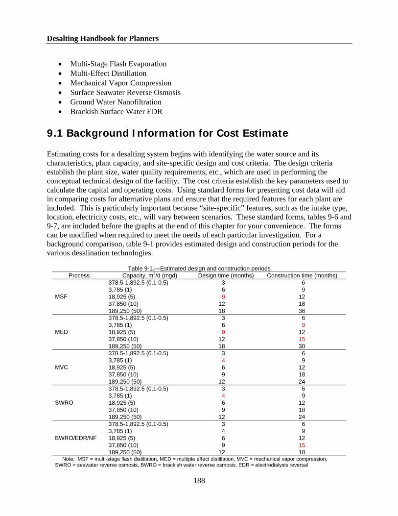
Desalting Handbook for Planners
188
• Multi-Stage Flash Evaporation • Multi-Effect Distillation • Mechanical Vapor Compression • Surface Seawater Reverse Osmosis • Ground Water Nanofiltration • Brackish Surface Water EDR
9.1 Background Information for Cost Estimate
Estimating costs for a desalting system begins with identifying the water source and its characteristics, plant capacity, and site-specific design and cost criteria. The design criteria establish the plant size, water quality requirements, etc., which are used in performing the conceptual technical design of the facility. The cost criteria establish the key parameters used to calculate the capital and operating costs. Using standard forms for presenting cost data will aid in comparing costs for alternative plans and ensure that the required features for each plant are included. This is particularly important because “site-specific” features, such as the intake type, location, electricity costs, etc., will vary between scenarios. These standard forms, tables 9-6 and 9-7, are included before the graphs at the end of this chapter for your convenience. The forms can be modified when required to meet the needs of each particular investigation. For a background comparison, table 9-1 provides estimated design and construction periods for the various desalination technologies.
Table 9-1.—Estimated design and construction periods Process Capacity, m3/d (mgd) Design time (months) Construction time (months)
378.5-1,892.5 (0.1-0.5) 3 6 3,785 (1) 6 9 18,925 (5) 9 12 37,850 (10) 12 18
MSF
189,250 (50) 18 36 378.5-1,892.5 (0.1-0.5) 3 6 3,785 (1) 6 9 18,925 (5) 9 12 37,850 (10) 12 15
MED
189,250 (50) 18 30 378.5-1,892.5 (0.1-0.5) 3 6 3,785 (1) 4 9 18,925 (5) 6 12 37,850 (10) 9 18
MVC
189,250 (50) 12 24 378.5-1,892.5 (0.1-0.5) 3 6 3,785 (1) 4 9 18,925 (5) 6 12 37,850 (10) 9 18
SWRO
189,250 (50) 12 24 378.5-1,892.5 (0.1-0.5) 3 6 3,785 (1) 4 9 18,925 (5) 6 12 37,850 (10) 9 15
BWRO/EDR/NF
189,250 (50) 12 18 Note: MSF = multi-stage flash distillation, MED = multiple effect distillation, MVC = mechanical vapor compression, SWRO = seawater reverse osmosis, BWRO = brackish water reverse osmosis, EDR = electrodialysis reversal

Chapter 9: Cost Estimating Procedures
189
9.2 Capital Cost
Capital cost (construction cost), as used in this document, refers to all costs associated with building the entire facility. In this sense, capital costs are often referred to as investment costs. The total capital (investment) cost estimate should represent a workable plant in place. Use tables 9-6 and 9-7 to record cost assumptions for your specific site. The same tables can be used for membrane process plants or distillation process plants. When cost detail is obtained from sources other than this chapter, supporting information should be shown in backup sheets.
9.2.1 Capital Cost Basis
The following cost basis was used for preparing the curves contained in this chapter.
Direct Capital Costs
The direct capital cost is the sum of:
• A desalting plant – distillation or membrane • Concentrate discharge piping and disposal • Pretreatment • Water intake structure • Feed water supply piping to the desalination units • Steam supply for distillation plants • Site preparation, paving, and grading • Post-treatment equipment • Process building for membrane systems • Auxiliary equipment
• Product storage • Emergency generators • Step-down transformer and control building for thermal systems • Product water distribution (high service) pumps • Process building for membrane systems
Indirect Capital Costs
Indirect costs are based on a percentage of direct capital costs. They include:
• Freight and insurance • Construction overhead • Owner’s direct expense • Contingency

Desalting Handbook for Planners
190
Depreciating Capital Costs
Depreciating capital costs are costs amortized over the life of the plant. They may include:
• Land cost • Working capital
Total Capital Cost is the sum of direct, indirect, and depreciating capital cost.
9.2.2 Annual Costs
The annual operating costs are for:
• Operations and maintenance labor • Chemicals • Energy • Supplies and maintenance materials • Replacement parts and membranes • Insurance • Fixed charges
Costs for these items are estimated for a 1-year period and divided by the quantity of water to be produced during the year to determine the overall cost of water. All of these charges, with the exception of insurance and fixed charges, depend on the amount of water produced. The plant factor, the percentage of time the plant is planned to be on-line, is used to adjust these dependent costs when calculating the annual cost of water.
9.3 Detailed Cost Estimates
9.3.1 Capital Costs
The following sections correspond to the items in tables 9-6 and 9-7. Use the cost parameters determined in each section to obtain cost from the indicated table. The total direct capital cost is the sum of items 9.3.1.1 – 9.3.1.10.

Chapter 9: Cost Estimating Procedures
191
9.3.1.1 Desalting Plant Costs
Multi-Stage Flash Distillation (MSF)
Figure 9-1 gives the total estimated construction cost for a complete MSF distillation system (recycle configuration). Total costs are given for a performance ratio1 of 3.44, 4.30, and 5.17 kilograms per mega joule (kg/MJ) (8, 10, and 12 lb of distillate/kBtu]). Figure 9-2 gives costs for the process only (for the plant proper) for the same performance ratios.
Multiple Effect Distillation (MED)
Figure 9-3 gives the total estimated construction cost for a MED plant. This cost assumes the low temperature, horizontal tube configuration. Total construction costs are given for performance ratios of 3.44, 4.30, and 5.17 kg/MJ (8, 10, and 12 lb/kBtu). Figure 9-4 shows the process-only capital costs for performance ratios of 3.44, 4.30, and 5.17 kg/MJ (8, 10, and 12 lb/kBtu).
Mechanical Vapor Compression (MVC)
Figure 9-5 gives the total estimated cost and cost basis for an MVC plant. Total costs are given for performance ratios of 3.44, 4.30, and 5.17 kg/MJ (8, 10, and 12 lb/kBtu). Figure 9-6 gives the process-only costs for the MVC process.
Seawater Reverse Osmosis (SWRO)
Figure 9-7 gives the total estimated construction cost for a SWRO plant with surface water feed. Figure 9-8 shows the total estimated construction cost for a SWRO plant using seawater wells, with a capacity limit of 10 million gallons per day (mgd) (37,850 m3/d). Using seawater wells to extract more than 20 mgd (75,700 m3/d) of feed water would normally not be considered feasible in the U.S. Total costs are based on single-pass plants, 50-percent recovery, 35,000 mg/l of total dissolved solids (TDS), and incorporating energy recovery devices.
Brackish Water Reverse Osmosis (BWRO)
Figure 9-7 gives the total estimated construction cost for a BWRO plant with surface water feed, and figure 9-8 gives the estimated construction cost for well water feed. Total construction costs are based on 75 percent recovery with no blending. The use of appropriately treated raw water for blending with the RO product will reduce the required RO capacity on a one-to-one basis. Raw water TDS is assumed to be 2,000 - 3,000 mg/l.
1 The performance ratio is the amount of water produced per unit of energy.

Desalting Handbook for Planners
192
Nanofiltration/Membrane Softening (NF)
Figure 9-7 gives the total estimated construction cost for a NF plant with surface water feed, and figure 9-8 gives the estimated construction cost with well water feed. Total construction costs assume an 85 percent recovery, feed water TDS of 750 mg/l, and with no blending.
Electrodialysis Reversal (EDR)
Figure 9-9 gives the total estimated construction cost for an EDR plant with surface and well water feed. Total construction costs assume an 80 percent recovery, with no blending. Cost curves are given for 3-stage (1,500-2,000 mg/l TDS feed water) and 4-stage (2,500-3,000 mg/l TDS feed water) systems. Each stage will remove approximately 50 percent of the TDS. A practical limitation on the capacity of EDR is about 57,000 m3/d (15 mgd). The Sarasota County, Florida, EDR plant, at 45,420 m3/d (12 mgd) is the largest example of this technology built to date.
9.3.1.2 Concentrate Disposal
This section describes the cost parameters for discharge costs. Mickley and Associates (2001) describe in detail several other methods for concentrate disposal with methods for determining costs.
Surface Water Discharge
In most cases, surface water discharge consists of a simple pipe. Cost is based on pipe length and diameter. Figure 9-10 gives construction costs for concentrate for distillation disposal. Pipeline costs will depend upon the distance of the plant from the disposal site. The charts are prepared for three distances: 457 m (1,500 ft); 762 m (2,500 ft); and 1,067 m (3,500 ft).
Figure 9-11 gives construction costs for surface water concentrate discharge for membrane systems. Pipeline costs for surface disposal will depend upon the distance to the discharge point. Three distances were chosen for estimating costs.
Disposal to Sewer
Where possible, this means of disposal is simple and usually cost effective. Factors that determine cost and feasibility are distance between the desalting plant and the sewage treatment plant, whether the two facilities are owned by the same entity, and future anticipated capacity increases.
Land Application
Cost depends on the loading rate, days of storage, cost of land, and the cost of clearing the land for planting. The values depend on the site, the evapo-transpiration rate, and the type of crops to be grown.

Chapter 9: Cost Estimating Procedures
193
Evaporation Ponds
Parameters for estimating costs of evaporation ponds are the cost of land, cost for excavation, area of the pond, height of the dike, and the liner thickness. These parameters depend on the evaporation rate, quality of the water, and capacity. Evaporation ponds and injection wells are assumed for brackish water systems only. Figure 9-12 gives costs for evaporation pond concentrate management for membrane systems.
Concentrate Concentrators for Zero Discharge
Costs depend on concentrate chemistry, energy usage, evaporator surface area, construction materials, and the need for chemical additives.
Deep-Well Injection
Deep-well injection is only appropriate where it is geologically feasible. The idea is to inject the concentrate down a well into a confined aquifer that cannot be used for drinking water or irrigation. The aquifer must not contact a fault and must be situated where there is little or no seismic activity. Cost depends on the diameter and depth of the well. The injection well costs are based on typical Florida injection well construction, with a 7,570 m3/d (2 mgd) capacity per well, and 100 percent redundancy. Figure 9-13 gives costs for deep-well injection of concentrate from membrane systems.
9.3.1.3 Pretreatment
Figure 9-14 gives the construction costs for pretreatment for distillation processes, which include chlorine disinfection, sodium bisulfate for dechlorination, acid, anti-foam, decarbonator, and deaerator. Construction cost for surface water pretreatment systems for membrane facilities includes chlorine disinfection, sodium bisulfate dechlorination, two-stage filtration, and sludge treatment. Figure 9-15 presents these costs.
9.3.1.4 Feed Water Intake
Seawater and Brackish Surface Water
An open intake was assumed for costing surface water systems. Figure 9-16 shows the construction cost for the intake for a distillation system. Figure 9-17 shows the construction cost for the intake for membrane systems.
Seawater and Brackish Well Water
Figure 9-18 gives costs for seawater and brackish well fields. Seawater wells are patterned after the Ranney method, with a yield of 15,140 m3/d (4 mgd) per collector. Brackish well field costs are based on 7,570 m3/d (2 mgd) per well, with a spacing of 305 m (1,000 ft). This includes submersible pumps, controls, security fence, and collection piping.

Desalting Handbook for Planners
194
9.3.1.5 Feed Water Pipe
Figure 9-19 gives the construction costs for various lengths of seawater intake pipes for distillation processes. Figure 9-20 gives the construction costs for the feed water intake for a seawater membrane plant for different lengths of pipe.
9.3.1.6 Steam Supply
Steam supply for distillation may be provided by a boiler that produces steam for the thermal desalting process. Backpressure turbines are used to produce steam for power and desalting in dual-purpose systems. Dual-purpose desalting systems offer attractive economics. However, evaluation of cost advantages requires a detailed study that is beyond the scope of this chapter. Cost data included in chapter 7 give a general insight into capital costs, steam costs, and electric power costs involved.
Figure 9-21 gives the construction costs for a boiler and controls (package boilers) for use with a single-purpose plant.
9.3.1.7 General Site Development
General site development includes excavation, site preparation, roads, and paving. Figure 9-22 shows costs for distillation site development, and figure 9-23 shows costs for membrane facilities.
9.3.1.8 Post-Treatment
Post-treatment for distillation includes caustic and lime addition for stabilization and chlorine for disinfection. Degasification is also included for post-treatment of membrane system product water. Figure 9-24 shows product post-treatment construction costs for distillation, and figure 9-25 shows product post-treatment costs for membrane systems.
9.3.1.9 Auxiliary Equipment
Auxiliary equipment includes product storage and transmission, step-down transformers for distillation processes, and emergency generators.
• Product storage tank construction costs are shown in figure 9-26 for distillation systems using steel tank construction and in figure 9-27 for membrane systems using prestressed concrete tank construction.
• Product transmission piping construction costs are shown in figure 9-28, for
pipeline lengths of 3,657 m, 7,315 m, and 14,630 m (12,000 ft, 24,000 ft, and 48,000 ft, respectively).

Chapter 9: Cost Estimating Procedures
195
• Emergency generator construction costs, including the fuel supply and piping, are given in figure 9-29. These costs assume the use of a diesel engine to drive the generator.
• Step-down transformer costs are shown in figure 9-30.
9.3.1.10 Building and Structures
Figure 9-31 gives construction costs for distillation buildings, and figure 9-32 gives construction costs for membrane systems for unit costs of $807, $1,076, and $1,614 per square meter ($75, $100, and $150 per square foot).
9.3.2 Indirect Capital Cost
Indirect, or depreciating, capital costs are based on a percentage of the direct capital cost calculated in section 9.3.1. Indirect capital costs include freight and insurance, interest during construction, construction overhead, owner’s expenses, and contingency. These costs are added to the direct capital cost to calculate the estimated total capital cost.
9.3.2.1 Freight and Insurance
The total construction costs do not include the shipping costs for delivering plant components to the site. For plants erected in the U.S., these costs are generally taken at 5 percent of the construction cost.
9.3.2.2 Interest During Construction
Interest during construction is computed on the basis that the owner borrows money as needed to finance construction and pays simple interest on this money after it is spent. The computation of this cost is simplified by assuming a constant rate of expenditure of funds over the construction time for the process selected and applying the interest rate to the direct capital costs for a period of one-half of the construction time.
9.3.2.3 Construction Overhead and Profit
The contractor’s overhead includes:
• Fringe benefits • Labor burden • Field supervisor • Temporary facilities • Construction equipment • Small tools • Miscellaneous

Desalting Handbook for Planners
196
Construction overhead is generally 15 percent of the direct capital costs for membrane systems. This percentage is modified for distillation processes using the adjustment factors in figure 9-33. The contractor’s profit is assumed at 3 percent.
9.3.2.4 Owner’s Direct Expense
The owner’s direct expenses include:
• Project investigation • Land acquisition • Engineering design • Contract administration • Legal expenses • Administrative expenses • Commissioning and/or startup costs
These costs vary considerably, depending on the owner’s method of accounting. The normal value is 10 percent of the direct capital costs, but this value depends on the specifics of a project and the size, both of which impact the total capital costs. Figure 9-33 shows adjustment factors.
The commissioning period is used to:
• Clean and flush piping • Check rotation of motor drivers • Perform hydrostatic testing • Set up and calibrate controls
Membrane systems also include:
• Disinfect the system • Load membranes
This period will require between 2 weeks and 6 months, depending upon the size, complexity, and number of units to be operated. The costs associated with commissioning are borne by the contractor as part of the total capital cost of the facility.
Startup costs are costs incurred by either the owner or the contractor. This period involves actual operation of the plant by conducting the performance and reliability testing. The duration of this period can be from 1 week to 1 month. During this time period, the contractor, equipment suppliers, and the owner will have personnel onsite. The costs for the owner’s personnel can be prorated from the annual labor cost for this facility. Note that there may be many more people and expenses during the startup.
9.3.2.5 Contingency
Contingency allocation is generally 10 percent of the direct capital cost.

Chapter 9: Cost Estimating Procedures
197
9.3.3 Nondepreciating Capital Costs
Nondepreciating capital costs are costs that do not lose value or expense, such as land and working capital cost.
9.3.3.1 Land
Figure 9-34 shows the land requirements for distillation process plants. These land requirements include roads and product storage areas. Local land costs should be used for pricing the site acquisition cost. Figure 9-35 shows the land requirements for membrane process plants.
9.3.3.2 Working Capital
Working capital is the ready cash on hand to cover the day-to-day expense of operating the facilities. This expense includes salaries (and salary overhead), chemicals, energy, maintenance materials, and insurance. For this item, an allowance of 2 months’ operating and maintenance cost is suggested. This allowance will result in a working capital cost of one-sixth of the total annual costs.
9.3.4 Annual Cost
Annual costs vary directly with the quantity of water produced. All costs are to be indexed to the price levels at the date of the estimate.
9.3.4.1 Labor
Figure 9-36 gives the annual labor costs for distillation processes, and figure 9-37 gives the annual labor costs for membrane processes. The labor category includes routine maintenance, as well as operations. Table 9-2 gives the total number of staff required for single and dual-purpose plants. Table 9-3 gives the total number of staff for surface and well water plants. These costs assume that the plant will be staffed 24 hours per day, 7 days per week for plants of 18,925 m3/d (5 mgd) and larger and 16 hours per day, 5 days per week for plants smaller than 18,925 m3/d (5 mgd). The actual staffing requirements will vary from State to State. The figures assume a labor rate of $25,000 per year.
Table 9-2.—Operations and maintenance staff – distillation processes
Capacity, m3/d (mgd) Process 3,785 (1) 18,925 (5) 30,280 (8) 37,850 (10) 189,250 (50)
Single purpose 14 14 18 20 35 Dual purpose 12 12 13 14 28

Desalting Handbook for Planners
198
Table 9-3.—Operations and maintenance staff – membrane processes Capacity, m3/d (mgd) Process
3,785 (1) 18,925 (5) 37,850 (10) 94,625 (25) 189,250 (50) SWRO 6 12 15 18 20 BWRO, EDR, NF 6 10 12 15 17
9.3.4.2 Chemicals
Figures 9-38, 9-39, and 9-40 give the annual costs for chemicals at distillation plants with performance ratios of 3.44, 4.30, and 5.17 kg/MJ (8, 10, and 12 lb/kBtu) for MSF, MED, and MVC, respectively. Figures 9-41 and 9-42 give the chemical costs for pretreatment, post-treatment, and cleaning for membrane systems for surface water and ground water sources, respectively. For more accurate estimates based on usage, the current unit cost of chemicals is listed in table 9-4.
Table 9-4.—Unit costs of chemicals by process and use
Process
Chemical
Use
Unit cost, $/kg ($/lb)
All Chlorine (1-ton cylinders) Pretreatment and post-treatment 0.49 (1.08)
All Lime (Quicklime) Post-treatment 0.17 (0.37)
All Caustic (50-percent solution) Post-treatment 0.75 (1.65)
Membrane Scale inhibitor Pretreatment 1.47 (3.24)
Distillation Anti-foam Pretreatment 1.21 (2.67)
All Sodium bisulfate Pretreatment 2.04 (4.50)
Thermal Polyphosphate Pretreatment 2.78 (6.13)
Distillation Ferric chloride Pretreatment 0.55 (1.21)
Distillation Corrosion inhibitor Post-treatment 0.88 (1.94)
All Sulfuric acid, 93 percent Pretreatment 0.11 (0.24) 9.3.4.3 Energy
Figures 9-43, 9-44, and 9-45 show the cost of electricity at $0.06/kWh for MSF, MED, and MVC, respectively. Figures 9-46 and 9-47 show membrane system costs for electricity at $0.06/kWh.
Steam
Steam costs for distillation vary not only with fuel costs and performance ratio but also with the plant type (i.e., single or dual-purpose). The dual-purpose plant steam costs also vary with the type of allocation cost method used to determine this cost.

Chapter 9: Cost Estimating Procedures
199
(a) Single-Purpose Plants
Figure 9-48 gives steam costs for single-purpose plants. These costs assume a performance ratio 5.17 kg/MJ (12 lb/kBtu heat input). These calculations assume a boiler efficiency of 85 percent for a range of fuel costs.
(b) Dual-Purpose Plants
The cost of steam from a dual-purpose plant has an economic advantage over a single- purpose plant because a dual-purpose plant uses fuel more efficiently. In a dual-purpose plant, steam produces some electrical energy before it is extracted for use in the desalting plant. Therefore, less fuel is consumed than would be required by two separate facilities in a typical single-purpose installation. Cost savings are also realized from using shared facilities in following areas:
• Seawater intake facilities • Concentrate disposal systems • Operation and maintenance labor • Maintenance shops and control room • Licensing and permitting
Cost allocation is used to:
• Present the costs of each product (i.e., water and electricity) • Determine the appropriate selling price of each product • Assist the planner in understanding the makeup of each production cost and,
therefore, in understanding the cost impacts for changes in design • Establish the basis for comparing different alternatives • Two methods of cost allocation generally are in use today: the “power credit” and
“available energy” methods. Figures 9-49 and 9-50 give the cost of steam, when using the power credit and available energy methods. For estimating purposes, the cost of electricity can be taken as that given at the start of this section.
Power Credit Method.—In the power credit method, the power production cost is charged with the plant and site costs resulting from constructing and operating only the power plant. The water plant is charged only with the cost of additional facilities, site work, fuel use, and operating expenses required for water production. The energy cost is determined by calculating the difference between the cost of power produced by the dual-purpose plant and the single-purpose plant. In this allocation method, the difference in power costs that results from constructing the dual-purpose plant is charged to the water production plant. The difference in cost depends on the amount of steam removed from

Desalting Handbook for Planners
200
the power cycle for desalination production and the pressure at which steam is extracted from the turbine.
Available Energy Method.—In the available energy method, costs are allocated to the electrical and water production, based on the energy that each use. In this method, the available energy is the energy that would be used for power production. (i.e., the enthalpy difference between the main steam pressure and the condensing pressure) and the power and water use. That is, the fraction of the steam cost attributed to power production is the ratio of the enthalpy drop across the turbine to the total enthalpy drop available for electrical power production in a single-purpose plant.
The unit cost of electrical product will, in each case, be greater than that for the base case (power production only).
9.3.4.4 Replacement Parts and Maintenance Materials
Figures 9-51, 9-52, and 9-53 give the annual costs for repairs and spare parts for performance ratios of 3.44, 4.30, and 5.17 kg/MJ (8, 10, and 12 lb/kBtu), respectively.
These costs assume 1 percent of the total capital costs for membrane systems for replacement parts and maintenance materials.
9.3.4.5 Membrane Replacement Cost
Figure 9-54 gives annual membrane replacement costs for SWRO, BWRO/NF, and EDR. These costs are calculated for the following desalting treatments:
• SWRO, $0.032/m3 ($0.12/kgal) • BWRO/NF, $0.021/m3 ($0.08/kgal) • EDR, $0.039/m3 ($0.15/kgal) for membranes, spacers, and stack parts
9.3.4.6 Insurance
Insurance costs assume 0.5 percent of total capital costs.
9.3.4.7 Annual Cost of Capital
The annual cost of depreciating capital normally includes the owner’s cost for interest amortization. The annual payment necessary to repay principal and interest in a present sum of money is called the Capital Recovery Factor. Table 9-5 lists the Capital Recovery Factors for different interest rates and amortization periods. Capital Recovery Factor, multiplied by total capital cost, is the payment each year for a loan at the indicated interest rate (i) and amortization period (y).

Chapter 9: Cost Estimating Procedures
201
CRFi i
i
y
y=+
+ −
*( )( ) ( )
11 1
Table 9-5.—Capital recovery factors
Repayment period (years) Interest rate 20 30 40
4.0 0.07358 0.05783 0.05052 4.5 0.07688 0.06139 0.05434 5.0 0.08024 0.06505 0.05828 5.5 0.08368 0.06881 0.06232 6.0 0.08718 0.07265 0.06646 6.5 0.09076 0.07658 0.07069 7.0 0.09439 0.08059 0.07501 7.5 0.09809 0.08467 0.07940 8.0 0.10185 0.08883 0.08386 8.5 0.10567 0.09305 0.08838 9.0 0.10955 0.09734 0.09296 9.5 0.11348 0.10168 0.09759
10.0 0.11746 0.10608 0.10226
9.3.4.8 Plant Factor
Plant factor is the amount of time (percent) the units will operate during the year at the percent of design capacity (i.e., onstream percent times percent of design capacity). For all cases, it is assumed that the desalination plants will operate at design capacity for 310 days per year (i.e., a plant factor of 85 percent). This allows ample time for preventive maintenance and unforeseen shutdowns.
References Chapman-Wilbert, M., 1998. “The Desalting and Water Treatment Membrane Manual: A Guide to Membranes for Municipal Water Treatment,” (2nd edition), Water Treatment Technology Program Report No. 29, Bureau of Reclamation, Denver, Colorado, 1998.
Mickley and Associates, 2001. “Membrane Concentrate Disposal Practices and Regulations,” Bureau of Reclamation, Desalination Water Purification Report Series No. 69, Denver, Colorado.

Desalting Handbook for Planners
202
Table 9-6a.—Design criteria
Item Requirement
Finished water quantity, m3/d (mgd)
Process capacity, m3/d (mgd)
Product water quality (mg/l)
Finished water quality (mg/l)
Distance to supply (m)
Number of trains
Design feed water temperature (oC)
Finished water quality goals: - Total hardness (as CaCO3) - Alkalinity (as CaCO3) - Langelier Saturation Index
Pump types and sizes: Intake or well pumps Feed pumps Transfer pumps Housekeeping pumps (cleaning, flushing, etc.) Product pumps High service pumps
Pretreatment method
Post-treatment method
Fresh water flush system type
Concentrate disposal method
Product storage tank size
Staffing requirements
Daily operational period
Disinfection equipment type

Chapter 9: Cost Estimating Procedures
203
Table 9-6b.—Economic criteria
Item Requirement
Cost year
Interest rate (percent)
Service life (years)
Plant factor (percent)
Electricity cost ($/kWh)
Steam cost $/MJ ($/Btu)
Labor rate ($/hour)
Labor overhead rate (percent)
Contingency (percent)
Contractor overhead and labor (percent)
Engineering and administration (percent)
Freight and insurance (percent)
Chemical costs ($/T): Acid Scale inhibitor Caustic Chlorine Sodium bisulfite Anti-foam Lime Coagulant Other
Membrane replacement (percent/year)
Repair and spare parts (percent/year)
Facility insurance (percent/year)
Land cost ($/hectare)

Desalting Handbook for Planners
204
Table 9-7.—Supporting sheet (sheet 1 of 3) Project: Date:
Project Description:
Project Type:
PRODUCT WATER CHARACTERISTICS Annual Requirement: Required Quality: Distance, Point of Delivery from Desalting Plant:
Required Reliability:
Facilities Required:
WATER SUPPLY CHARACTERISTICS Physical Description: Chemical Description:
Other:
Facilities Required:
DESALTING COMPLEX CHARACTERISTICS Process Being Considered: Replaceable Items: Frequency of Replacement (years): Concentrate Disposal Requirements:
Service Required at Source:
Cost of Services Purchased: Fuel: Steam: Electric Power:
Auxiliary Facilities Required:

Chapter 9: Cost Estimating Procedures
205
Table 9-7.—Computation sheet (sheet 2 of 3) Project Description: Project:
Date:
Desalting Plant Capacity in m3/d
Process Capital Costs
Concentrate Disposal Capital Costs
Pretreatment Capital Costs
Intake Capital Costs
Feed Water Supply Piping Capital Costs
Boiler Capital Costs
Site Development Costs
Post-Treatment Capital Costs
Auxiliary Capital Costs
Building Capital Costs
Interest During Construction
Land Cost
Annual Labor Costs
Annual Chemical Costs
Annual Steam Costs
Annual Electric Power Costs
Annual Repairs and Spares Costs
Other Computations

Desalting Handbook for Planners
206
Table 9-7.—Cost summary (sheet 3 of 3) Project Description: Project:
Date: Price Level:
Desalting Plant - Type: Capacity (m3/d): Annual Plant Factor (percent): Interest Rate (percent): Annual Production (m3): Plant Life (years): Capital Recovery Factor:
CAPITAL COSTS
Capital Cost Centers Est. Cost ($) 1. Desalting Plant 2. Concentrate Disposal 3. Pretreatment 4. Water Intake 5. Feed Water Pipes 6. Steam Supply 7. General Site Development 8. Post-Treatment 9. Auxiliary Equipment (product storage, product transmission, step-down transformers, emergency generators)
10. Building and Structures Subtotal Direct Capital Cost (DCC) 11. Freight and Insurance 5 percent of DCC 12. Interest During Construction (DCC x Interest Rate x One Half of Construction Time (Table 9.1) in years) 13. Construction Overhead 15 percent of DCC x factor from figure 9-33 14. Owner’s Direct Expense 10 percent of DCC x factor from figure 9-33 15. Contingency 10 percent of DCC Total - Depreciating Capital 16. Land Costs 17. Working Capital (1/6 x items 18-24) Total - Nondepreciating Capital Total Capital Costs
ANNUAL COSTS Annual Cost Centers Est. Cost ($/yr) 18. Operation and Maintenance Labor 19. Chemicals 20. Steam 21. Electric Power 22. Supplies, Maintenance, and Insurance 23. Insurance Total Operation and Maintenance 24. Annual Costs - Depreciating Capital 25. Annual Costs - Nondepreciating Capital Total Annual Capital Charges 26. Annual Replacement Costs Total Annual Costs
COST OF WATER (Total Annual Costs/ Yearly Production)

Chapter 9: Cost Estimating Procedures
207
Figure 9-1 Total construction cost—MSF process
1
10
100
1,000
1,000 10,000 100,000 1,000,000
Plant Capacity (m3/day)
Con
stru
ctio
n C
ost (
$1,0
00,0
00 -
2000
)
PR=5.17 kg/MJ (12 lbs/kBtu) PR=4.30 kg/MJ (10 lbs/kBtu) PR=3.44 kg/MJ (8 lbs/kBtu)
Construction Costs Include: Desalting Plant ProperInterstage PipingPumps, Motors and ControlsSeawater SupplyPretreatmentPost TreatmentBuildingCleaning System Electrical DistributionIndirect Cost
Plant Type: RecycleOperating Temperature: 110 C (235 F)Configuration: Cross-Tube
Construction Costs do not Include:Land CostsProduct Water DeliveryBoiler
Figure 9-2 Process construction cost—MSF
1
10
100
1,000
1,000 10,000 100,000 1,000,000
Plant Capacity (m3/day)
Con
stru
ctio
n C
ost (
$1,0
00,0
00 -
2000
)
PR=5.17 kg/MJ (12 lbs/kBtu) PR=4.30 kg/MJ (10 lbs/kBtu) PR=3.44 kg/MJ (8 lbs/kBtu)
Plant Type: RecycleOperating Temperature: 110 C (235 F)Configuration: Cross-Tube
Costs Include:Desalting Plant ProperInterstage Piping & ValvesPumps, Motors and ControlsCleaning System Electrical Distribution Costs do not Include:
PretreatmentIntake System Post TreatmentBuildingAuxiliary EquipmentStorage & Delivery Systems Land CostsBoilerIndirect Cost

Desalting Handbook for Planners
208
Figure 9-3 Total construction cost—MED process
10
100
1,000
1,000 10,000 100,000 1,000,000
Plant Capacity (m3/day)
Con
stru
ctio
n C
ost (
$1,0
00,0
00 -
2000
)
PR=5.17 kg/MJ (12 lbs/kBtu) PR=4.30 kg/MJ (10 lbs/kBtu) PR=3.44 kg/MJ (8 lbs/kBtu)
Construction Costs Include:Desalting Plant ProperInterstage PipingPumps, Motors and ControlsSeawater SupplyBuildingPretreatmentPost TreatmentElectrical DistributionCleaning System Indirect Cost
Plant Type: Horizontal TubeOperating Temperature: 71.1 C (160 F)
Construction Costs do not Include:Land CostsProduct Water DeliveryBoiler
Figure 9-4 Process construction cost—MED
1
10
100
1,000
1,000 10,000 100,000 1,000,000Plant Capacity (m3/day)
Con
stru
ctio
n C
ost (
$1,0
00,0
00 -
2000
)
PR=5.17 kg/MJ (12 lbs/kBtu) PR=4.30 kg/MJ (10 lbs/kBtu) PR=3.44 kg/MJ (8 lbs/kBtu)
Costs Include:Desalting Plant ProperInterstage PipingPumps, Motors and ControlsCleaning System Electrical Distribution
Construction Costs do not Include:PretreatmentPost TreatmentIntake SystemAuxiliary EquipmentLand CostsBuildingBoilerStorage & Delivery SystemsIndirect Cost

Chapter 9: Cost Estimating Procedures
209
Figure 9-6 Process construction cost - MVC
1
10
100
1,000 10,000 100,000
Plant Capacity (m3/day)
Con
stru
ctio
n C
ost (
$1,0
00,0
00 -
2000
)
PR=5.17 kg/MJ (12 lbs/kBtu) PR=4.30 kg/MJ (10 lbs/kBtu) PR=3.44 kg/MJ (8 lbs/kBtu)
Costs Include:Desalting Plant ProperInterstage PipingPumps, Motors and ControlsElectrical Distribution Construction Costs do not Include:
PretreatmentPost TreatmentAuxiliary EquipmentProduct Water Storage and DeliveryLand CostsBuildingBoilerIntake SystemIndirect Cost
Figure 9-5 Total constuction cost - MVC process
1
10
100
1,000
1,000 10,000 100,000 1,000,000
Plant Capacity (m3/day)
Con
stru
ctio
n C
ost (
$1,0
00,0
00 -
2000
)
PR=5.17 kg/MJ (12 lbs/kBtu) PR=4.30 kg/MJ (10 lbs/kBtu) PR=3.44 kg/MJ (8 lbs/kBtu)
Costs Include:Desalting Plant Proper Interstage PipingPumps, Motors and ControlsSeawater SupplyPretreatmentPost TreatmentCleaning SystemElectrical DistributionBuildingIndirect Cost
Plant Type: Mechanical Vapor CompressorOperating Temperature: 107.2 C (225 F)
Construction Costs do not Include:Land CostsProduct Water DeliveryConcentrate Disposal

Desalting Handbook for Planners
210
Figure 9-7 Total construction cost—SWRO, BWRO, and NF plants with surface water feed
Figure 9-8 Total construction cost—SWRO, BWRO, and NF plants with well water feed
1
10
100
1,000
1,000 10,000 100,000 1,000,000Plant Capacity (m3/day)
Con
stru
ctio
n C
ost (
$1,0
00,0
00 -
2000
)
SWRO BWRO NF
Construction Costs Include:Desalting Plant ProperInplant pipingPumps, Motors and ControlsPretreatmentPost TreatmentBuildingCleaning SystemElectrical DistributionIndirect Cost
Construction Costs do not Include:Land CostsProduct Water DeliveryConcentrate Disposal
1
10
100
1,000 10,000 100,000 1,000,000Plant Capacity (m3/day)
Con
stru
ctio
n C
ost (
$1,0
00,0
00 -
2,00
0)
SWRO BWRO NF
Construction Costs Include:Desalting Plant ProperInplant PipingPumps, Motors and ControlsPost TreatmentBuildingCleaning SystemElectrical DistributionIndirect Costs
Costs do not Include:Land CostsProduct Water Delivery Concentrate Disposal

Chapter 9: Cost Estimating Procedures
211
Figure 9-10 Construction cost—concentrate disposal pipeline for distillation processes
0.1
1
10
1,000 10,000 100,000 1,000,000Plant Capacity (m3/day)
Con
stru
ctio
n C
ost (
$1,0
00,0
00 -
2000
)
Disposal Point 457 m (1,500 ft) Disposal Point 762 m (2,500 ft) Disposal Point 1,067 m (3,500 ft)
Costs Include:Disposal Pipeline
Costs do not Include:Indirect Costs
Figure 9-9 Total construction cost - EDR plant
1
10
100
1,000 10,000 100,000
Plant Capacity (m3/day)
Con
stru
ctio
n C
ost (
$1,0
00,0
00 -
2000
)
3 stage SW 4 stage SW 3 stage GW 4 stage GW
Construction Costs Include:Desalting Plant ProperInplant PipingPumps, Motors and ControlsBrackish Water SupplyBuildingPost TreatmentElectrical DistributionCleaning SystemIndirect Cost
Construction Costs do not Include:Land CostsProduct Water DeliveryConcentrate disposal

Desalting Handbook for Planners
212
Figure 9-11 Construction cost—concentrate disposal pipeline for membrane processes
0.01
0.10
1.00
10.00
1,000 10,000 100,000 1,000,000
Plant Capacity (m3/day)
Con
stru
ctio
n C
ost (
$1,0
00,0
00 -
2000
)
SWRO 1500ft SWRO 3000ft SWRO 4500ft BW/EDR/NF 3000ft BW/EDR/NF 1500ft BW/EDR/NF 4500ft
Costs Include:Disposal Pipeline
Costs do not Include:Indirect Costs
Figure 9-12 Construction cost—evaporation ponds for membrane processes
1
10
100
1,000
1,000 10,000 100,000 1,000,000
Plant Capacity (m3/day)
Con
stru
ctio
n C
ost (
$1,0
00,0
00 -
2000
)
Cost estimate based on:Net Evaporation rate of 127 cm/yr. (50"/yr)Duplicate cells50% freeboard85% plant factor
Cost estimate does not include:Land costIndirect costs
14.17 hectares (35 acres)
141.65 hectares (350 acres)
70.82 hectares (175
354.11 hectares (875 acres)
708.22 hectares (1750 acres)

Chapter 9: Cost Estimating Procedures
213
Figure 9-13 Construction cost—-injection wells for membrane processes
1.0
10.0
100.0
1,000 10,000 100,000 1,000,000
Plant Capacity (m3/day)
Con
stru
ctio
n C
ost (
$1,0
00,0
00 -
2000
)
Costs Include:WellsRedundant WellWellhead equipment
Costs do not Include:Indirect Costs
Figure 9-14 Construction cost - pretreatment for distillation processes
0.1
1
10
1,000 10,000 100,000 1,000,000
Plant Capacity (mgd)
Con
stru
ctio
n C
ost (
$1,0
00,0
00 -
2000
)
Costs Include:Chlorine TreatmentSodium Bisulfite TreatmentAcid TreatmentAnti-Foam TreatmentDecarbonatorDeaerator
Costs do not Include:Indirect Costs

Desalting Handbook for Planners
214
0.1
1.0
10.0
100.0
1,000 10,000 100,000 1,000,000
Plant Capacity (m3/day)
Con
stru
ctio
n C
ost (
$1,0
00,0
00 -
2000
)
Costs Include:Chlorine TreatmentSodium Bisulfite TreatmentTwo-stage FiltrationSludge treatment
Costs do not Include:Indirect Costs
Figure 9-15 Construction cost—surface water pretreatment for membrane processes
Figure 9-16 Construction cost—open intake for distillation processes
0.10
1.00
10.00
1,000 10,000 100,000 1,000,000
Plant Capacity (m3/day)
Con
stru
ctio
n C
ost (
$1,0
00,0
00 -
2000
)
MSF Open Intake Open Intake MED Open Intake MVC
Construction Costs Include:Intake ChannelIntake StructureTraveling Screens & Trash RacksPumps, Motors and Controls
Costs do not Include:Indirect Costs

Chapter 9: Cost Estimating Procedures
215
Figure 9-17 Construction cost—open intake systems for smaller membrane processes
Figure 9-18 Total construction cost—wellfields
0.1
1
10
100
1,000 10,000 100,000 1,000,000
Plant Capacity (m3/day)
Con
stru
ctio
n C
ost (
$1,0
00,0
00 -
2000
)
SWRO BW-400ft BW-600ft BW-800ftCosts Include:WellsPumping EquipmentElectrical & ControlsWellhouseLateral pipingCollector piping
Construction Costs do not Include:Land CostsWell Water Delivery
Brackish wells assumed to have depths of 200, 400, 600, 800ft
0.1
1
10
1,000 10,000 100,000 1,000,000Plant Capacity (m3/day)
Con
stru
ctio
n C
ost (
$1,0
00,0
00 -
2000
)
SWRO BWRO
Construction Costs Include:Intake ChannelIntake StructureTraveling Screens & Trash RacksPumps, Motors and Controls
Note: Use BWRO costs for EDR and NF
Costs do not Include:Indirect Costs

Desalting Handbook for Planners
216
Figure 9-20 Construction cost - seawater feed water pipeline for membrane processes
Figure 9-19 Construction cost—seawater feed water pipeline for distillation processes
0.1
1
10
1,000 10,000 100,000 1,000,000
Plant Capacity (m3/day)
Con
stru
ctio
n C
ost (
$1,0
00,0
00 -
2000
) )
Pipe Length 457 m (1,500 ft) Pipe Length 762 m (2,500 ft) Pipe Length 1,067 m (3,500 ft) Pipe Length 1,372 m (4,500 ft)
0.1
1
10
1,000 10,000 100,000 1,000,000
Plant Capacity (m3/day)
Con
stru
ctio
n C
ost (
$1,0
00,0
00 -
2000
)
Pipe Length 457 m (1,500 ft) Pipe Length 762 m (2,500 ft)Pipe Length 1,067 m (3,500 ft) Pipe Length 1,372 m (4,500 ft)

Chapter 9: Cost Estimating Procedures
217
Figure 9-21 Construction cost – package boilers for single-purpose plant
0.1
1
10
1,000 10,000 100,000 1,000,000Plant Capacity (m3/day)
Con
stru
ctio
n C
ost (
$1,0
00,0
00 -
2000
)
Costs Include:BoilerControls
Costs do not Include:Indirect Costs
Figure 9-22 Construction cost - site development for distillation processes
0.01
0.1
1
1,000 10,000 100,000 1,000,000
Plant Capacity (m3/day)
Con
stru
ctio
n C
ost (
$1,0
00,0
00 -
1999
)
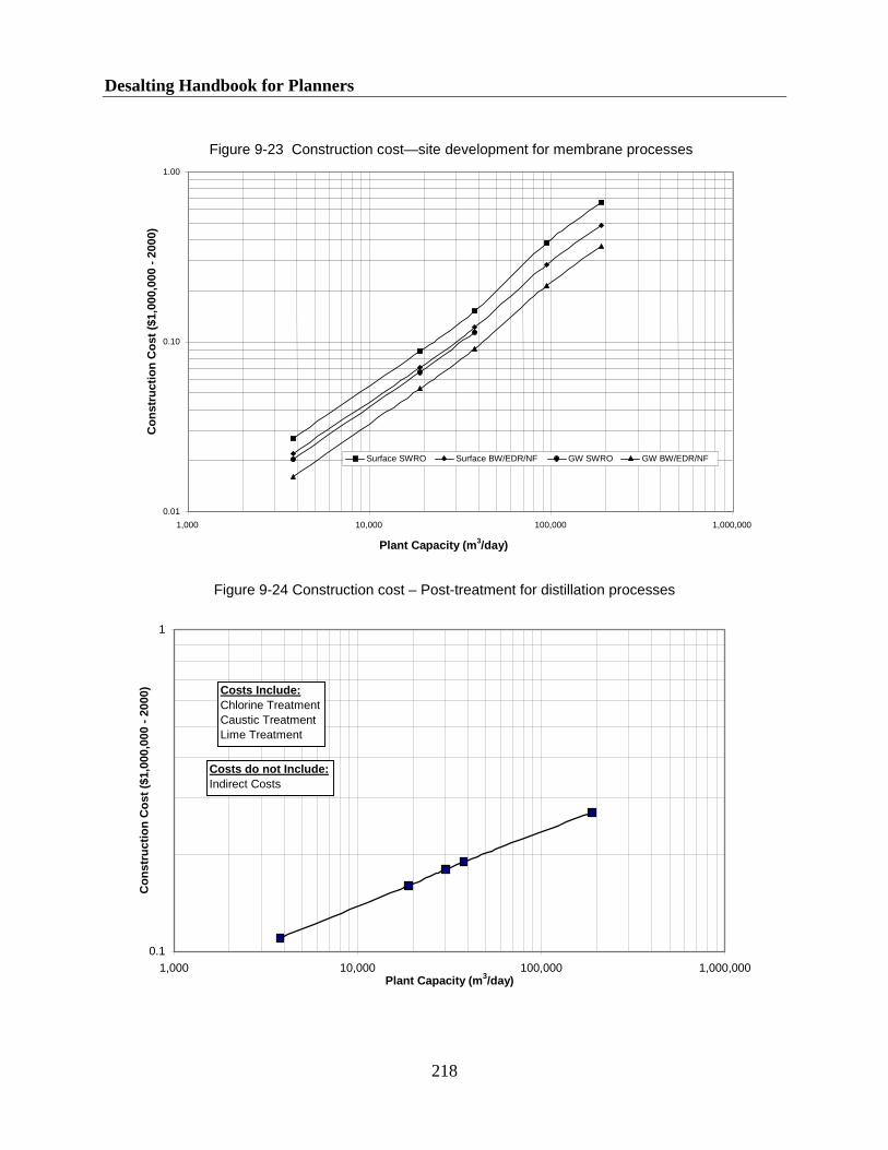
Desalting Handbook for Planners
218
Figure 9-24 Construction cost – Post-treatment for distillation processes
Figure 9-23 Construction cost—site development for membrane processes
0.01
0.10
1.00
1,000 10,000 100,000 1,000,000
Plant Capacity (m3/day)
Con
stru
ctio
n C
ost (
$1,0
00,0
00 -
2000
)
Surface SWRO Surface BW/EDR/NF GW SWRO GW BW/EDR/NF
0.1
1
1,000 10,000 100,000 1,000,000Plant Capacity (m3/day)
Con
stru
ctio
n C
ost (
$1,0
00,0
00 -
2000
) Costs Include:Chlorine TreatmentCaustic TreatmentLime Treatment
Costs do not Include:Indirect Costs

Chapter 9: Cost Estimating Procedures
219
Figure 9-26 Construction cost – product storage for distillation systems using steel tank construction
0.1
1
10
1,000 10,000 100,000 1,000,000Storage Capacity (m3)
Con
stru
ctio
n C
ost (
$1,0
00,0
00 -
2000
)
Costs Include:Product Storage Sized for Full Day Capacity
Costs do not Include:Indirect Costs
Figure 9-25 Construction cost—post-treatment for membrane systems
0.1
1.0
10.0
1,000 10,000 100,000 1,000,000
Plant capacity (m3/day)
Con
stru
ctio
n C
ost (
$1,0
00,0
00 -
2000
)
Costs Include: Degassification pH adjustment Disinfection, NaOCl Corrosion Inhibitor Costs Do Not Include: Indirect Costs Fluoride

Desalting Handbook for Planners
220
Figure 9-28 Construction cost – product transmission pipeline
Figure 9-27 Construction cost—product storage for membrane systems using prestressed concrete tank construction
0.10
1.00
10.00
1,000 10,000 100,000 1,000,000
Plant Capacity (m3/day)
Con
stru
ctio
n C
ost (
$1,0
00,0
00 -
2000
)
Costs Include:Storage for one day's production
Costs do not Include:Indirect Costs
0.1
1
10
100
1,000 10,000 100,000 1,000,000Plant Capacity (m3/day)
Con
stru
ctio
n C
ost (
$1,0
00,0
00 -
2000
)
Transmission Length 3,657 m (12,000 ft) Transmission Length 7,315 m (24,000 ft)Transmission Length 14,630 m (48,000 ft)
Costs Include:High Service PumpingTransmission Pipeline Length as shownBuilding
Costs do not Include:Indirect Costs
Assumes Pipeline InstallationCost at $27.89/m ($8.50/ lineal foot)

Chapter 9: Cost Estimating Procedures
221
Figure 9-29 Construction cost – emergency generators
Figure 9-30 Construction cost – step-down transformers
0.01
0.1
1
1,000 10,000 100,000 1,000,000Plant Capacity (m3/day)
Con
stru
ctio
n C
ost (
$1,0
00,0
00 -
2000
)
Costs Include:Diedel GeneratorFuel TankSpill Containment
Costs do not Include:Indirect Costs
0.1
1
10
1,000 10,000 100,000 1,000,000Plant Capacity (m3/day)
Con
stru
ctio
n C
ost (
$1,0
00,0
00 -
2000
)
Costs Include:Step-down TranformersInstallation
Costs do not Include:Indirect Costs

Desalting Handbook for Planners
222
Figure 9-31 Construction cost—distillation process buildings
0.01
0.10
1.00
10.00
1,000 10,000 100,000 1,000,000
Plant Capacity (m3/day)
Con
stru
ctio
n C
ost (
$1,0
00,0
00 -
2000
)
$807.00/m2 ($75.00/sf) $1,076/m2 ($100.00/sf) $1,614/m2 ($150.00/sf)
Figure 9-32 Construction cost—membrane process buildings
0.1
1.0
10.0
1,000 10,000 100,000 1,000,000Plant Capacity (m3/day)
Con
stru
ctio
n C
ost (
$1,0
00,0
00 -
2000
)
SWRO$807.00/m2 ($75.00/sf) SWRO$1,076/m2 ($100.00/sf) SWRO$1,614/m2 ($150.00/sf)BW$807.00/m2 ($75.00/sf) BW$1,076/m2 ($100.00/sf) BW$1,614/m2 ($150.00/sf)

Chapter 9: Cost Estimating Procedures
223
Figure 9-33 Owner’s direct expense and COH factors
0.80
0.85
0.90
0.95
1.00
1.05
1.10
1.15
1.20
1.25
1.30
0 10 20 30 40 50 60 70
Project Construction Cost ($1,000,000 - 2000)
Indi
rect
Cos
t Adj
ustm
ent F
acto
r
Owner's Cost Factor COH Cost Factor
Base Case:Owner's Expense -10% of Construction CostCOH - 15% of Construction Cost
Figure 9-34 Land requirements—for distillation process plants
0.001
0.01
0.10
1.00
10.00
1,000 10,000 100,000 1,000,000Plant Capacity (m3/day)
Land
Req
uire
men
t (he
ctar
e)
Total Land Requirement Process Land Site LandBuilding Land

Desalting Handbook for Planners
224
Figure 9-36 Annual cost—labor for distillation process
0.10
1.00
1,000 10,000 100,000 1,000,000
Plant Capacity (m3/day)
Ann
ual C
ost (
$1,0
00,0
00 -
2000
)
All Processes Single Purpose All Processes Dual Purpose
0.01
0.10
1.00
10.00
1,000 10,000 100,000 1,000,000
Plant Capacity (m3/day)
Land
Req
uire
men
t (he
ctar
es)
Surface SWRO Surface BW, NF, EDR Wellwater SWRO Groundwater BW, NF, EDR
Figure 9-35 Land requirements—for membrane process plants
1 hectare=2.471 acres

Chapter 9: Cost Estimating Procedures
225
Figure 9-37 Annual cost – labor for membrane processes
0.1
1
1,000 10,000 100,000 1,000,000
Plant Capacity (m3/day)
Ann
ual L
abor
Cos
t ($1
,000
,000
- 20
00)
SWRO BWRO/EDR/NF
Figure 9-38 Annual cost - MSF chemicals
0.1
1
10
100
1,000 10,000 100,000 1,000,000
Plant Capacity (m3/day)
Ann
ual C
ost (
$1,0
00,0
00 -
1999
) PR=5.17 kg/MJ (12 lbs/kBtu) PR=4.30 kg/MJ (10 lbs/kBtu)PR=3.44 kg/MJ (8 lbs/kBtu)

Desalting Handbook for Planners
226
Figure 9-39 Annual cost - MED chemicals
0.1
1
10
100
1,000 10,000 100,000 1,000,000
Plant Capacity (m3/day)
Ann
ual C
ost (
$1,0
00,0
00 -
1999
)
PR=5.17 kg/MJ (12 lbs/kBtu) PR=4.30 kg/MJ (10 lbs/kBtu)PR=3.44 kg/MJ (8 lbs/kBtu)
Figure 9-40 Annual cost - MVC chemicals
0.01
0.1
1
1,000 10,000 100,000
Plant Capacity (m3/day)
Ann
ual C
ost (
$1,0
00,0
00 -
2000
)
PR=5.17 kg/MJ (12 lbs/kBtu) PR=4.30 kg/MJ (10 lbs/kBtu)
PR=3.44 kg/MJ (8 lbs/kBtu)

Chapter 9: Cost Estimating Procedures
227
Figure 9-42 Annual cost—chemicals for ground water membrane processes
0.01
0.10
1.00
10.00
1,000 10,000 100,000 1,000,000Plant Capacity (m3/day)
Ann
ual C
hem
ical
Cos
t ($1
,000
,000
- 20
00)
BWRO EDR NF SWRO
Figure 9-41 Annual cost—chemicals for surface water membrane processes
0.01
0.10
1.00
10.00
1,000 10,000 100,000 1,000,000Plant Capacity (m3/day)
Ann
ual C
hem
ical
Cos
t ($1
,000
,000
- 20
00)
BWRO EDR NF SWRO

Desalting Handbook for Planners
228
Figure 9-44 Annual cost – MED processes electricity
0.1
1.0
10.0
100.0
1,000 10,000 100,000 1,000,000Plant Capacity (m3/day)
Ann
ual C
ost (
$1,0
00,0
00 -
2000
)
PR=3.44 kg/MJ PR=4.30 kg/MJ PR=5.17 kg/MJ
Power @ $0.06/kWh
Figure 9-43 Annual cost - MSF processes electricity
100
1,000
10,000
100,000
1,000 10,000 100,000 1,000,000
Plant Capacity (m3/day)
Elec
tric
al C
onsu
mpt
ion
(kW
)
PR=3.44 kg/MJ PR=4.30 kg/MJ PR=5.17 kg/MJ

Chapter 9: Cost Estimating Procedures
229
Figure 9-45 Annual cost—MVC processes electricity
Figure 9-46 Annual cost—SWRO processes electricity
0.10
1.00
10.00
100.00
1,000 10,000 100,000 1,000,000
Plant Capacity (m3/day)
Ann
ual E
lect
rical
Cos
t ~$1
,000
,000
/yr
Surface Intake Beach Wells
Surface Water Power Cost includes:Power for intake pumpsPower for pre-treated water pumpsProcess powerDistribution (high service) pump powerBuilding services
Groundwater Cost includes:Power for well pumpsProcess powerDistribution pump powerBuilding services
1
10
100
1,000
1,000 10,000 100,000 1,000,000Plant Capacity (m3/day)
Ann
ual C
ost (
$1,0
00,0
00 -
2000
)
PR=3.44 kg/MJ PR=4.30 kg/MJ PR=5.17 kg/MJ
Power @ $0.06/kWh

Desalting Handbook for Planners
230
Figure 9-48 Annual cost—steam for single-purpose plants
0.1
1.0
10.0
100.0
1,000 10,000 100,000 1,000,000
Plant Capacity (m3/day)
Ann
ual C
ost (
$1,0
00,0
00 -
2000
)
Fuel Cost at $947.00/MJ ($1.00/MMBtu) Fuel Cost at $1,894.00/MJ ($2.00/MMBtu)Fuel Cost at $2841.00/MJ ($3.00/MMBtu) Fuel Cost at $3788.00/MJ ($4.00/MMBtu)
Basis:Performance Ratio=5.17 kg/MJ(12 lbs/kBtu)Boiler Efficiency=85%
Figure 9-47 Annual cost—BWRO, EDR, and NF plant electricity
0.01
0.10
1.00
10.00
1,000 10,000 100,000 1,000,000
Plant Capacity (m3/day)
Ann
ual E
lect
rical
Cos
t $1
,000
,000
/yr
BWRO-Surface EDR-Surface BWRO-Ground NF-Ground NF-Surface EDR-Ground
Surface Water Cost includes:Power for intake pumpsPower for pre-treated water pumpsProcess powerDistribution pump powerBuilding services
Groundwater Cost includes:Power for well pumpsProcess powerDistribution pump powerBuilding services

Chapter 9: Cost Estimating Procedures
231
Figure 9-49 Annual cost—steam for dual-purpose plants, power credit method
0.0
0.1
1.0
10.0
100.0
1,000 10,000 100,000 1,000,000
Plant Capacity (m3/day)
Ann
ual C
ost (
$1,0
00,0
00 -
2000
)
Fuel Cost at $947.00/MJ ($1.00/MMBtu) Fuel Cost at $1,894.00/MJ ($2.00/MMBtu)Fuel Cost at $2841.00/MJ ($3.00/MMBtu) Fuel Cost at $3788.00/MJ ($4.00/MMBtu)
Figure 9-50 Annual cost—steam for dual-purpose plants, available energy method
0.0
0.1
1.0
10.0
100.0
1,000 10,000 100,000 1,000,000
Plant Capacity (m3/day)
Ann
ual C
ost (
$1,0
00,0
00 -
2000
)
Fuel Cost at $947.00/MJ ($1.00/MMBtu) Fuel Cost at $1,894.00/MJ ($2.00/MMBtu)Fuel Cost at $2841.00/MJ ($3.00/MMBtu) Fuel Cost at $3788.00/MJ ($4.00/MMBtu)

Desalting Handbook for Planners
232
Figure 9-51 Annual cost — MSF repairs and spares
0.10
1.00
10.00
1,000 10,000 100,000 1,000,000Plant Capacity (m3/day)
Ann
ual C
ost (
$1,0
00,0
00 -
2000
)
PR=5.17 kg/MJ (12 lbs/kBtu) PR=4.30 kg/MJ (10 lbs/kBtu) PR=3.44 kg/MJ (8 lbs/kBtu)
Figure 9-52 Annual cost—MED repairs and spares
0.10
1.00
10.00
1,000 10,000 100,000 1,000,000
Plant Capacity (m3/day)
Ann
ual C
ost (
$1,0
00,0
00 -
2000
)
PR=5.17 kg/MJ (12 lbs/kBtu) PR=4.30 kg/MJ (10 lbs/kBtu) PR=3.44 kg/MJ (8 lbs/kBtu)

Chapter 9: Cost Estimating Procedures
233
Figure 9-53 Annual cost—MVC repairs and spares
Figure 9-54 Annual cost—membrane replacement
0.01
0.10
1.00
10.00
1,000 10,000 100,000 1,000,000
Plant Capacity (m3/day)
Ann
ual C
ost (
$1,0
00,0
00 -
2000
)
SWRO BWRO/NF EDR
0.1
1
1,000 10,000 100,000
Plant Capacity (m 3/day)
Ann
ual C
ost (
$1,0
00,0
00 -
2000
)
PR=5.17 kg/ MJ (12 lbs/ kBt u) PR=4.30 kg/ MJ (10 lbs/ kBt u) PR=3.44 kg/ MJ (8 lbs/ kBt u)


Appendix A: Reclamation’s Desalting Program
A-1
Appendix A: Reclamation’s Desalting Program
A.1 Historical Background
The U.S. Department of the Interior, Bureau of Reclamation (Reclamation) has a long history in desalination. Federal funding of desalination research began in 1952, with the passage of the Saline Water Act. Over the next 30 years, Congress appropriated over $1 billion in today’s dollars for research, development, and demonstration projects. The visionary goals of cost effectively converting saline and brackish water into usable water were advanced through the Department of the Interior. The Office of Saline Water (OSW) was created in 1954, and the subsequent Office of Water Research and Technology (OWRT) was formed in 1974. These programs were primarily responsible for reverse osmosis (RO) technology development and for many breakthroughs and improvements in thermal technologies. Today’s widespread use of desalination would not be possible had it not been for these programs. They were, in retrospect, incredibly farsighted in providing research and development stimulus to desalination at a time when few land-based water supply problems were even identified in the U.S. Research provided benefits in other technology fields, such as the advent of kidney dialysis using membranes. Reclamation became involved in desalination as a testing laboratory for OSW developments. In this role, Reclamation conducted verification testing both in-house and in the field, as well as supervised many pilot projects for OSW. Pilot testing conducted at field sites in Roswell, New Mexico, and Dalpra Farm, Colorado, evaluating membrane technology, provided Reclamation with pioneering in-depth capabilities in desalination. In the 1970s, Reclamation became directly involved when legislation for evaluating options for desalinating agricultural return flows in the irrigation valley in southwestern Arizona was introduced. Salinity issues in this area mandated action in order to conform to treaty obligations with Mexico. In time, this led to the world’s largest membrane desalination facility, Reclamation’s Yuma Desalting Plant. Though this plant has never operated for long term at full capacity, it is maintained in a standby status. The Water Quality Improvement Center was subsequently created at this facility and is used for research, technology transfer, and training activities to further desalination and water reuse technologies. Federal funding for desalination activities largely stopped in the early 1980s, when OWRT was abolished as a result of redirected congressional funding. The remaining desalination program was transferred to Reclamation, due to its ongoing activities in relation to the Yuma Desalting Plant. In the early and mid-1990s, approximately $1.3 million per year for desalination research funding was appropriated for Reclamation under the Water Treatment Technology Program. In 1996, Senator Paul Simon was responsible for passage of the Water Desalination Act of 1996. This Act authorized program funding of $5 million per year for research and studies for 6 years, beginning with fiscal year 1998. In addition, $25 million was authorized over six years for demonstration projects. Reclamation has received appropriations as shown in table A-1, since the passage of the Act. It must be reauthorized by Congress in order for appropriations to be made after fiscal year 2002.

Desalting Handbook for Planners
A-2
Table A-1.—Summary of appropriations under the Water Desalination Act of 1996
Fiscal year Appropriated funds (million $)
1998 2.70 1999 1.50 2000 0.65 2001 1.30 2002 4.00 Total 10.15
A.2 Reclamation’s Present Program and Accomplishments
The primary goal of Reclamation’s Desalination Research and Development Program is to develop more cost-effective and technologically efficient means to desalinate water. To accomplish this, Reclamation is forming partnerships with private industry, universities, local communities, non-governmental organizations, and others to address a broad range of desalting and water purification needs. The primary thrusts of the program, as outlined by the Water Desalination Act of 1996, are to:
• Perform research on desalination technologies and related issues to push the state-of-the-art forward (Research and Studies).
• Conduct development and demonstration activities to verify advancements, to confirm
economics, and to gain public acceptance (Demonstration).
• Research is conducted through grants and contracts with non-Federal entities. The Federal share of the cost of the research, study, or demonstration project shall not exceed 25 percent unless the Secretary of the Interior determines that the project is not feasible without the increased Federal contribution and then not exceed 50 percent of the total cost of the project.
To attain the primary goal, the following objectives were established for Reclamation’s Desalination Research and Development Program:
• Increase the ability of communities of varying sizes and financial resources to economically treat saline water to potable standards.
• Increase the ability of the United States desalination industry to compete throughout the
world, by fostering partnerships with them for the development of new and innovative technologies.

Appendix A: Reclamation’s Desalting Program
A-3
• Develop methods to make desalting more efficient through promotion of dual-use facilities in which waste energy could be applied to desalting water.
• Develop methods to ensure desalting technologies are environmentally friendly. • Ensure regulations are appropriate for the application by working with regulators to fully
evaluate the effects of concentrate streams. • Capitalize on the recovery of by-product streams. • Maximize technology transfer to ensure full transfer of knowledge and commercialization
of technology. Since the initial funds were appropriated for this program in fiscal year 1998, approximately 60 assistance agreements have been awarded to private industry, universities, and research organizations. The following findings and accomplishments resulted:
• Membrane bioreactors successfully treat screened and degritted sewage so that it is suitable for further treatment with desalting technology. This represents a ‘step-change’ in treatment technology by providing a smaller footprint, higher quality sludge residuals, and a much higher quality product. Membrane bioreactors have a cost advantage over conventional treatment methods, and they have less of an environmental impact.
• Various advancements in membrane materials and technology have been made. A better
understanding of membrane fouling has been described by several researchers, leading to increased membrane life, reduced chemical cleanings, reduced impact on the environment, and reduced capital and operation and maintenance costs. In addition, there is strong indication that chlorine resistance in a thin film composite membrane has been achieved in a project co-funded by Reclamation and the U.S. Army.
• Several projects showed advancements in pretreatment of water for application with
desalting membranes. In one case, specially submerged pipes on a beach were used to filter seawater. In another case, biological pretreatment of saline water did an excellent job of pretreating feedwater. A third case in progress, low-pressure membrane filtration (e.g., microfiltration) as pretreatment for seawater RO, has the potential to significantly improve performance and reliability. All of these techniques have a lower environmental impact than conventional pretreatment technologies. Larger scale studies are needed in order to estimate the cost savings associated with using these new technologies.
• An advanced high-pressure seawater pump was developed that reduces energy
consumption over 35 percent, compared to similar pumps using conventional energy recovery. Since energy consumption for seawater RO and the amortized capital associated with energy recovery equal about 50 percent of the total water cost, this could provide a significant overall cost savings.

Desalting Handbook for Planners
A-4
• An innovative, low-cost system using evaporation technology was developed. This can be constructed and operated by unskilled laborers. This system uses low-grade heat to produce high quality water with very little operator involvement. This technology is suitable for relatively low volume product water, such as rural communities. The lower capital and operational costs make this technology ideal for communities that cannot afford RO technology.
Each of these findings is being recommended to Congress for additional funding for larger scale demonstration testing. In addition, the desalination community and potential desalination users have developed several significant tools for use. These include:
• An abstract database of all the desalination literature has been completed in partnership with the American Water Works Association (AWWA). The database includes a full-text database of all Federal Government desalination reports (approximately 1,200 reports funded by OSW and OWRT written from 1954-1982) and various full-text conference proceedings and abstracts.
• The first edition of a computerized desalination cost model has been developed in
partnership with the American Membrane Technology Association (AMTA) and the National Institute of Standards and Technology (NIST).
This Desalting Handbook for Planners was created to assist in the decision-making process for potential desalination users. Reclamation also wrote a comprehensive membrane manual that has been distributed around the world to the desalination and membrane community. In addition, this manual is used by the Electric Power Research Institute (EPRI) and has been sent to all of their member utilities. Currently, all final reports of desalination research activities funded by Reclamation are available to the public in hardcover, on CDROM, and are available from the program’s website <www.usbr.gov/water/desal.html>. Additionally, numerous technology transfer activities and workshops intended to promote further development of desalination technology have been sponsored by Reclamation. These have included the following:
• “Growing the U.S. Water Supply through Purification Technologies” – A workshop held in Golden, Colorado, April, 2000, to discuss and develop a consensus regarding purification technologies. Participants included the water resources community, representatives from national organizations, various State/local water organizations, and industry, as well as congressional representatives.

Appendix A: Reclamation’s Desalting Program
A-5
• Membrane Research Needs Workshop – A workshop held in July 2000, co-sponsored by the American Water Works Association Research Foundation (AWWARF) to develop a broad-based outline of the research needs of all membrane technologies. Participants included national and international membrane experts and municipal representatives.
• Desalination Research and Development Workshop – A workshop held in January 2001,
co-sponsored by the National Water Research Institute (NWRI), focused on prioritizing the most significant issues that need to be addressed now to speed the installation of cost-effective desalination facilities. Participants included national desalination experts and users.
Reclamation is also the co-founder of the Interagency Consortium for Desalination and Membrane Separation Research (Consortium). This Consortium was established in 1992 to provide a communications network for the exchange of information between Federal Government agencies involved in desalination and membrane research. Consortium members work together to gain the following benefits:
• Prevent Federal duplication of effort • Pool limited Federal research funding and other resources to obtain common goals • Identify future research needs • Allow for discussion of new technologies with other experts in the field
Federal agencies and laboratories that have participated in the yearly Consortium activities since its inception include:
• U.S. Army • Center for Health Promotion & Preventative Medicine • Corps of Engineers: Cold Regions Research Engineering Lab • Corps of Engineers: Construction Engineering Research Laboratory • Tank-Automotive & Armaments Command Mobility Tech Center (TACOM) • Yuma Proving Ground • Center for Disease Control (CDC) • Defense Advanced Research Projects Agency (DARPA) • Bureau of Reclamation • U.S. Geological Survey • Department of Energy • Office of Fossil Energy • Federal Energy Technology Center • Office of Nuclear Energy • Environmental Protection Agency • National Aeronautic and Space Administration (NASA) - Marshall Space Flight Center • Department of Agriculture • National Institute of Standards and Technology (NIST) • U.S. Navy

Desalting Handbook for Planners
A-6
• Command Control and Ocean Surveillance Center • Naval Facilities Engineering Service Center • Naval Surface Warfare Center • Naval Command Control and Ocean Surveillance Center
These activities, combined with a balanced and comprehensive research studies and pilot projects program, have resulted in steady gains towards the program goal of more cost-effective and efficient means to desalinate water. The U.S. water supply is becoming more stressed as competing demands grow for the limited existing freshwater supplies. Desalination is one of the few methods by which to augment this supply and, thereby, reduce this stress. It is critical that the U.S. continue to create and develop desalination technologies and continue to work towards more cost-effective desalination technologies. Equally important, it is paramount that partnerships be forged between the different interest groups—those needing desalination, the regulators, community leaders, and those focused on environmental priorities—to achieve acceptable water supply solutions with which all citizens can live.


C-1
Appendix C: ASTM Standards Applicable to Membrane Systems
Published standards under the jurisdiction of ASTM Committee D19 on Water and the direct responsibility of Subcommittee D19.08 on Membranes and Ion Exchange Materials
Number Date Title
D3739-94 1998 Standard Practice for Calculation and Adjustment of the Langelier Saturation Index for Reverse Osmosis
D3923-94 1998 Standard Practices for Detecting Leaks in Reverse Osmosis Devices
D4189-95 2002 Standard Test Method for Silt Density Index (SDI) of Water
D4194-95 2001 Standard Test Methods for Operating Characteristics of Reverse Osmosis Devices
D4195-88 1998el Standard Guide for Water Analysis for Reverse Osmosis Application
D4472-89 1998el Standard Guide for Record Keeping for Reverse Osmosis Systems
D4516-00 Standard Practice for Standardizing Reverse Osmosis Performance Data
D4582-91 2001 Standard Practice for Calculation and Adjustment of the Stiff and Davis Stability Index for Reverse Osmosis
D4692-01 ND Standard Practice for Calculation and Adjustment of Sulfate Scaling Salts (CaSO4, SrSO4, and BaSO4) for Reverse Osmosis and Nanofiltration
D4993-89 1998el Standard Practice for Calculation and Adjustment of Silica (SiO2) Scaling for Reverse Osmosis
D5090-90 2001 Standard Practice for Standardizing Ultrafiltration Permeate Flow Performance Data
D5091-95 2001 Standard Guide for Water Analysis for Electrodialysis/Electrodialysis Reversal Applications
D5131-90 2001 Standard Guide for Record Keeping for Electrodialysis/Electrodialysis Reversal Systems
D6161-98 2002 Standard Terminology Used for Crossflow Microfiltration, Ultrafiltration, Nanofiltration, and Reverse Osmosis Membrane Processes
Contact: ASTM, 100 Barr Harbor Drive, West Conshohocken PA, 19428-295 <http://www.astm.org/>

D-1
Appendix D: Worked Examples
D-1 Multi-Stage Flash Evaporation D-2 Multi-Effect Distillation D-3 Mechanical Vapor Compression D-4 Surface Seawater Reverse Osmosis D-5 Low TDS Brackish Surface Water EDR D-6 Ground Water Nanofiltration


Appendix D: Worked Examples
D-3
D-1 Multi-Stage Flash Evaporation
This is an estimate for a Multi-Stage Flash Evaporation (MSF) plant to furnish 30 x 106 m3 per year of supplemental water to the City of Greener Pastures. The single-purpose plant will be located 1000 meters from the Pacific Ocean and will use seawater for feed. The City has sufficient water storage capacity in its present system, and product water from the desalting plant can be introduced into the water distribution system at the plant site. Oil is available at the site at an average price of $2,841 per mega joule. Electric power is available at the site at a price of $0.09 per kilowatthour. An oil-fired boiler will be required. The City plans to finance construction by a bond issue and estimates the average interest rate on bonds to be 7 percent. An allowance for taxes is not required, and land cost is $74,130 per hectare. Note: Amortization is 30 years at 7 percent; annual insurance cost is 0.5% of total depreciable capital; performance ratio = 5.17 kilograms distillate per mega joule (12 pounds per 1000 British thermal units)

Desalting Handbook for Planners
D-4
Supporting Sheet Project Description: Supplemental Water Supply for City of Greener Pastures Project: SP-1
Date: 1/2001
PRODUCT WATER CHARACTERISTICS Annual Requirement: 30 x 106 m3
Required Quality: < 500 mg/l TDS Distance Point of Delivery from Desalting Plant: At plant
Required Reliability: 90% at design capacity
Facilities Required: Surface intake, pretreatment, desalting plant, post-treatment
WATER SUPPLY CHARACTERISTICS Physical description: Seawater TDS = 34,500 mg/l
Chemical Description:
Other:
DESALTING COMPLEX CHARACTERISTICS Process Being Considered: MSF Replaceable Items: Normal maintenance Frequency of Replacement (yrs): N/A Concentrate Disposal Requirements: Pipeline back to sea Performance Ratio: 5.17 kg distillate/MJ
Service Required at Source: N/A
Cost of Services Purchased: Fuel: $2,841/MJ Electric Power: $0.09/kWh
Auxiliary Facilities Required: Step-down transformer
OTHER NOTES

Appendix D: Worked Examples
D-5
Computation Sheet Project Description: Supplemental water supply for the city of Greener Pastures. Costs to include seawater intake, pretreatment, desalting plant, post-treatment, and steam boiler. It is proposed to use MSF.
Desalting Plant Capacity: 30 x 106 m3/yr ÷ (365 d/yr x 0.90) = 91,500 m3/d
Process Capital Costs: From Figure 9-2: $130,000,000
Concentrate Disposal Capital Costs: From Figure 9-10: $1,300,000
Pretreatment Capital Costs: From Figure 9-14: $2,600,000
Intake Capital Costs: From Figure 9-16: $5,200,000
Feed Water Supply Piping Capital Costs: From Figure 9-19: For 762 m = $2.1 M; For 1000 m = $2,100,000 x 1000/762 m = $2,760,000
Boiler Capital Costs: From Figure 9-21: $1,100,000
Site Development Costs: From Figure 9-22: $470,000
Post-Treatment Capital Costs: From Figure 9-24: $230,000
Auxiliary Equipment Capital Costs: Includes Step-Down Transformer: $650,000
Building Capital Costs: From Figure 9-31: $1,000,000 @ $1,076/m2
Interest During Construction: Direct Capital Cost x Interest Rate x One Half of Construction Time (Table 9.1) in years = $145,310,000 x .07 x (1/2) x 2 = $10,172,000
Land Cost: From Figure 9-34: 1.2 hectares x $74,130 / hectare = $89,000
Annual Labor Costs: From Figure 9-36: $680,000
Annual Chemical Costs: From Figure 9-38: $5,100,000
Annual Steam Costs: From Figure 9-48: $18,000,000
Annual Electric Power Costs: From Figure 9-43: $5,550,000 @ $0.09/kWh
Annual Repairs and Spares Costs: From Figure 9-51: $4,300,000
Other Computations: Step-Down Transformer: From Figure 9-30: $650,000

Desalting Handbook for Planners
D-6
Cost Summary Project Description: Desalting plant facility for the City of Greener Pastures
Desalting Plant - Type: MSF Capacity (m3/d): 91,500
Annual Plant Factor (percent): 90 Interest Rate (percent): 7
Annual Production (m3): 30 x 106 Plant Life (years): 30
Capital Recovery Factor: 0.0806
CAPITAL COSTS
Capital Cost Centers Est. Cost ($) 1. Desalting Plant 130,000,000
2. Concentrate Disposal 1,300,000
3. Pretreatment 2,600,000
4. Water Intake 5,200,000
5. Feed Water Pipes 2,760,000
6. Steam Supply 1,100,000
7. General Site Development 470,000
8. Post-Treatment 230,000
9. Auxiliary Equipment (step-down transformers) 650,000
10. Building and Structures 1,000,000
Subtotal Direct Capital Cost (DCC) 145,310,000
11. Freight and Insurance 5 percent of DCC 7,266,000
12. Interest During Construction (DCC x Interest Rate x One Half of Construction Time (Table 9.1) in years)
10,172,000
13. Construction Overhead 15 percent of DCC x factor from figure 9-33 (.95) 20,707,000
14. Owner’s Direct Expense 10 percent of DCC x factor from figure 9-33 (.9) 13,078,000
15. Contingency 10 percent of DCC 14,531,000
Total - Depreciating Capital 211,064,000
16. Land Costs 89,000
17. Working Capital (1/6 x items 18-23) 5,785,000
Total - Nondepreciating Capital 5,874,000
Total Capital Costs 216,938,000
ANNUAL COSTS
Annual Cost Centers Est. Cost ($/yr)
18. Operation and Maintenance Labor 680,000
19. Chemicals 5,100,000
20. Steam 18,000,000
21. Electric Power 5,550,000
22. Repairs and Spares 4,300,000
23. Insurance (.5% of total depreciating capital) 1,077,000
Total Operation and Maintenance 34,707,000
24. Annual Costs - Depreciating Capital (Total-Depreciating Capital x 0.0806) 17,012,000
25. Annual Costs - Nondepreciating Capital (Total- Nondepreciation Capital x 0.0806) 473,000
Total Annual Capital Charges 17,485,000
26. Annual Membrane Replacement Costs N/A
Total Annual Costs (Total O & M and Capital Charges) 52,192,000
COST OF WATER (Total Annual Costs/ Yearly Production) $1.74/m3

Appendix D: Worked Examples
D-7
D-2 Multi-Effect Distillation
This is an estimate for a Multi-Effect Distillation (MED) desalting plant to furnish 30 x 106 m3 per year of supplemental water to the Greater Metro Utility District. The plant will be located 1000 meters from the Pacific Ocean and will use seawater for feed. The District has sufficient water storage capacity in its present system. Product water will be delivered to one of the District’s storage reservoirs, some 3000 meters from the plant site. Plant reliability is not considered critical. The District plans to build this desalting plant adjacent to its new Big Rock power plant and utilize steam from the power plant. Fixed charges on investment are expected to be 7 percent interest. Fuel costs for Big Rock are expected to be $1,894 per mega joule for the 500-megawatt unit. The available heat method is employed to determine steam costs. Electrical power is available at $0.03 per kilowatthour.
Note: Amortization is 30 years at 7 percent; annual insurance cost is 0.5% of total capital costs; performance ratio = 5.17 kilograms distillate per mega joule (12 pounds per 1000 British thermal units); land cost = $74,130 per hectare

Desalting Handbook for Planners
D-8
Supporting Sheet Project Description: Supplemental Water Supply for Greater Metro Utility District. It is proposed to use MED.
PRODUCT WATER CHARACTERISTICS Annual Requirement: 30 x 106 m3
Required Quality: to SDWA Distance Point of Delivery from Desalting Plant: 3000 m
Required Reliability: 90% at design capacity
Facilities Required: Seawater intake, pretreatment, desalting process, steam supply, post-treatment, and delivery to distribution system
WATER SUPPLY CHARACTERISTICS Physical Description: Seawater TDS=34,500 mg/l
Chemical Description:
Other:
Facilities Required:
DESALTING COMPLEX CHARACTERISTICS Process Being Considered: MED Replaceable Items: Normal preventive maintenance Frequency of Replacement (yrs): N/A Concentrate Disposal Requirements: Pipeline back to sea, 1000 m Performance Ratio: 5.17 kg distillate/MJ
Service Required at Source: N/A
Cost of Services Purchased: Fuel: $1,894/MJ Steam: Use available energy allocation method Electric Power: $0.03/kWh
Auxiliary Facilities Required: Step-down transformer, product transmission
OTHER NOTES

Appendix D: Worked Examples
D-9
Computation Sheet Project Description: Desalting Plant for Greater Metro Utility District
Desalting Plant Capacity: 30 x 106 m3/yr ÷ (365 d/yr x 0.90) = 91,500 m3/d
Process Capital Costs: From Figure 9-4: $75,000,000
Concentrate Disposal Capital Costs: From Figure 9-10: $1,300,000
Pretreatment Capital Costs: From Figure 9-14: $2,600,000
Intake Capital Costs: From Figure 9-16: $4,700,000
Feed Water Supply Piping Capital Costs: From Figure 9-19: $2,500,000
Boiler Capital Costs: N/A
Site Development Costs: From Figure 9-22: $490,000
Post-Treatment Capital Costs: From Figure 9-24: $230,000
Auxiliary Capital Costs: Includes product transmission and step-down transformer: $6,950,000
Building Capital Costs: From Figure 9-31: $1,300,000 @ $1076/m2
Interest During Construction: Direct Capital Cost x Interest Rate x One Half of Construction Time (Table 9.1) in years = $95,070,000 x .07 x (1/2) x 2 = $6,655,000
Land Cost: From Figure 9-34: 1.3 hectares by $74,130/hectare = $96,400
Annual Labor Costs: From Figure 9-36: $500,000
Annual Chemical Costs: From Figure 9-39: $4,900,000
Annual Steam Costs: From Figure 9-50: 3,600,000
Annual Electric Power Costs: From Figure 9-44: $1,600,000 @ $0.03/kWh
Annual Repairs and Spares Costs: From Figure 9-52: $2,800,000
Other Computations: Product Transmission Capital Costs: From Figure 9-28: $6,300,000 Step-Down Transformer Cost: From Figure 9-30: $650,000

Desalting Handbook for Planners
D-10
Cost summary Project Description: Desalting Plant for Greater Metro Utility District
Desalting Plant - Type: MED Capacity (m3/d): 91,500
Annual Plant Factor (percent): 90% Interest Rate (percent): 7
Annual Production (m3): 30 x 106 Plant Life (years): 30
Capital Recovery Factor: 0.0806
CAPITAL COSTS
Capital Cost Centers Est. Cost ($) 1. Desalting Plant 75,000,000
2. Concentrate Disposal 1,300,000
3. Pretreatment 2,600,000
4. Water Intake 4,700,000
5. Feed Water Pipes 2,500,000
6. Steam Supply N/A
7. General Site Development 490,000
8. Post-Treatment 230,000
9. Auxiliary Equipment (step-down transformer, product transmission)
6,950,000
10. Building and Structures 1,300,000
Subtotal Direct Capital Cost (DCC) 95,070,000
11. Freight and Insurance 5 percent of DCC 4,754,000
12. Interest During Construction (DCC x Interest Rate x One Half of Construction Time (Table 9.1) in years)
6,655,000
13. Construction Overhead 15 percent of DCC x factor from figure 9-33 (.95) 13,547,000
14. Owner’s Direct Expense 10 percent of DCC x factor from figure 9-33 (.90) 8,556,000
15. Contingency 10 percent of DCC 9,507,000
Total - Depreciating Capital 138,089,000
16. Land Costs 96,400
17. Working Capital (1/6 x items 18-23) 2,348,000
Total - Nondepreciating Capital 2,444,000
Total Capital Costs 140,533,000
ANNUAL COSTS
Annual Cost Centers Est. Cost ($/yr)
18. Operation and Maintenance Labor 500,000
19. Chemicals 4,900,000
20. Steam 3,600,000
21. Electric Power 1,600,000
22. Repairs and Spares 2,800,000
23. Insurance (.5% of total depreciating capital) 690,000
Total Operation and Maintenance 14,090,000
24. Annual Costs - Depreciating Capital (Total-Depreciating Capital x 0.0806) 11,130,000
25. Annual Costs - Nondepreciating Capital (Total- Nondepreciating Capital x 0.0806) 197,000
Total Annual Capital Charges 11,327,000
26. Annual Membrane Replacement Costs N/A
Total Annual Costs (Total O & M and Capital Charges) 25,417,000
COST OF WATER (Total Annual Costs/ Yearly Production) $ 0.85/m3

Appendix D: Worked Examples
D-11
D-3 Mechanical Vapor Compression
This is an estimate for a Mechanical Vapor Compression (MVC) desalting plant to furnish 1.24 x 10⁶ m3 per year of supplemental water to the City of Great Hope. The plant is located 800 meters from the Atlantic Ocean and will use seawater for feed. The water produced from the plant will be pumped to the City’s water storage tank, 7 kilometers from the water treatment plant site. The MVC plant will be a single-purpose facility, taking its steam from a packaged boiler located onsite. Fuel costs are expected to be $2,841 per mega joule for the boiler. Electricity will be taken from the adjacent electrical grid at a cost of $0.04 per kilowatthour.
Note: Amortization is 30 years at 7 percent; annual insurance cost is 0.5% of total capital costs; performance ratio = 5.17 kilograms distillate per mega joule; land cost = $50,000 per hectare

Desalting Handbook for Planners
D-12
Supporting Sheet
Project Description: Supplemental Water Supply for the City of Great Hope
PRODUCT WATER CHARACTERISTICS Annual Requirement: 1.24 x 10⁶ m3 Required Quality: <500 mg/l TDS Distance Point of Delivery from Desalting Plant: 7 kilometers
Required Reliability: 90% at design capacity
Facilities Required: Seawater intake, pretreatment, desalting plant, post-treatment, boiler, and concentrate disposal to ocean.
WATER SUPPLY CHARACTERISTICS Physical Description: Seawater TDS = 34,500 mg/l
Chemical Description:
Other: Land Cost at $50,000/hectare
Facilities Required: See above
DESALTING COMPLEX CHARACTERISTICS Process Being Considered: MVC Replaceable items: Normal maintenance Frequency of Replacement (yrs): N/A Concentrate Disposal Requirements: Pipeline back to sea Performance Ratio: 5.17 kg distillate/MJ
Service Required at Source: N/A
Cost of Services Purchased: Fuel: $2,841/MJ Steam: Electric Power: $0.04/kWh
Auxiliary Facilities Required: Emergency generator, product transmission
OTHER NOTES:

Appendix D: Worked Examples
D-13
Computation Sheet Project Description: Water Supply for the City of Great Hope Desalting Plant Capacity: 1.24 x 10⁶ ÷ (365 day/yr x 0.90) = 3,775 m3/d Process Capital Costs: Figure 9-6: $5,500,000 Concentrate Disposal Capital Costs: Figure 9-10: $200,000 Pretreatment Capital Costs: Figure 9-14: $290,000 Intake Capital Costs: From Figure 9-16: $380,000 Feed Water Supply Piping Capital Costs: From Figure 9-19: $410,000 Boiler Capital Costs: Figure 9-21: $170,000 Site Development Costs: Figure 9-22: $30,000 Post-Treatment Capital Costs: Figure 9-24: $120,000 Auxiliary Capital Costs: Includes Product Transmission, Step-Down Transformer, and Emergency Generator: $1,932,000 Building Capital Costs: Figure 9-31: $40,000 @ $807/m2 Interest During Construction: Direct Capital Cost x Interest Rate x One Half of Construction Time (Table 9.1) in years = $9,072,000 x 0.07 x (1/2) x (9/12) = $238,140 Land Cost: Figure 9-34: 0.05 hectares x $50,000/hectare = $2,500 Annual Labor Costs: Figure 9-36: $360,000 Annual Chemical Costs: Figure 9-40: $24,000/yr Annual Steam Costs: Figure 9-48 ($2,841/MJ): $750,000/yr. Annual Electric Power Costs: Figure 9-45 @ $0.04/kWh: $800,000 Annual Repairs and Spares: Figure 9-53: $180,000 Other Computations: Product Transmission Capital Costs: Figure 9-28: $1,800,000 Emergency Generator Cost: Figure 9-29: $12,000 Step-Down Transformer Cost: Figure 9-30: $120,000

Desalting Handbook for Planners
D-14
Cost Summary Project Description: Desalting plant for the City of Great Hope
Desalting Plant - Type: MVC Capacity (m3/d): 3,775
Annual Plant Factor (percent): 90 Interest Rate (percent): 7
Annual Production (m3): 1.24 x 10⁶ Plant Life (years): 30
Capital Recovery Factor: 0.0806
CAPITAL COSTS
Capital Cost Centers Est. Cost ($) 1. Desalting Plant 5,500,000
2. Concentrate Disposal 200,000
3. Pretreatment 290,000
4. Water Intake 380,000
5. Feed Water Pipes 410,000
6. Steam Supply 170,000
7. General Site Development 30,000
8. Post-Treatment 120,000
9. Auxiliary Equipment (product transmission, step down transformer, emergency generator)
1,932,000
10. Building and Structures 40,000
Subtotal Direct Capital Cost (DCC) 9,072,000
11. Freight and Insurance 5 percent of DCC 453,600
12. Interest During Construction (DCC x Interest Rate x One Half of Construction Time (Table 9.1) in years) 238,140
13. Construction Overhead 15 percent of DCC x factor from figure 9-33 (1.01) 1,374,000
14. Owner’s Direct Expense 10 percent of DCC x factor from figure 9-33 (1.12) 1,016,000
15. Contingency 10 percent of DCC 907,200
Total - Depreciating Capital 13,061,000
16. Land Costs 2,500
17. Working Capital (1/6 x items 18-23) 363,167
Total - Nondepreciating Capital 365,667
Total Capital Costs 13,427,000
ANNUAL COSTS
Annual Cost Centers Est. Cost ($/yr)
18. Operation and Maintenance Labor 360,000
19. Chemicals 24,000
20. Steam 750,000
21. Electric Power 800,000
22. Repairs and Spares 180,000
23. Insurance 65,000
Total Operation and Maintenance 2,179,000
24. Annual Costs - Depreciating Capital (Total-Depreciating Capital x 0.0806) 1,053,000
25. Annual Costs - Nondepreciating Capital (Total- Nondepreciating Capital x 0.0806) 29,473
Total Annual Capital Charges 1,082,000
26. Annual Membrane Replacement Costs N/A
Total Annual Costs (Total O & M and Capital Charges) 3,261,000
COST OF WATER (Total Annual Costs/ Yearly Production) $2.63/m3

Appendix D: Worked Examples
D-15
D-4 Surface Seawater Reverse Osmosis
The coastal City of Happy Beach needs to increase its municipal water capacity to accommodate rapid growth in its service district. After several studies, it has been concluded that seawater desalination provides the highest level of reliability, at reasonable cost. The plant will be located within a city park approximately 1,000 meters from the ocean, will use an existing sewer outfall for concentrate discharge, and will have a rated capacity of 20,000 m3 per day (5.4 million gallons per day). Water will be transferred by product pumps to an existing storage tank from an underground clearwell located on the site. Distance to the City tank is 3,000 meters.
Note: Amortization is 20 years at 6 percent; annual insurance cost is 0.5% of total capital costs

Desalting Handbook for Planners
D-16
Design Criteria
Item Requirement
Finished water quantity, m3/d (mgd) 20,000 (5.4)
Process capacity, m3/day (mgd) 20,000 (5.4)
Product water quality (mg/L) <500
Finished water quality (mg/L) <500
Distance to supply (m) 3000
Number of trains 3
Design feed water temperature (oC) 22
Finished water quality goals: - Total hardness (as CaCO3) - Alkalinity (as CaCO3) - Langelier index
50 50 ±0.2
Pump types and sizes: Intake or well pumps Feed pumps Transfer pumps Housekeeping pumps (Cleaning, flushing, etc.) Product pumps High service pumps
4 vertical turbine wet pit, 556 m3/hr 3 horizontal multi-stage - - 3 horizontal split can, 417 m3/hr -
Pretreatment method Conventional
Post-treatment method CO2/Lime/Corrosion Inh./Chlorine
Fresh water flush system type Permeate Flush
Concentrate disposal method Existing Sewer Outfall
Product storage tank size 20,000 m3
Staffing requirements 1 superintendent, 4 shift operators
Daily operational period 24 hours
Disinfection equipment type Sodium Hypochlorite

Appendix D: Worked Examples
D-17
Economic Criteria Item Requirement
Cost year 2002
Interest rate (%) 6
Service life (yrs) 20
Plant factor (%) 90
Electricity cost ($/kWh) 0.095
Steam cost $/MJ ($/Btu) -
Labor rate ($/yr) 25,000
Labor overhead rate (%) Inc.
Contingency (%) 10
Contractor overhead and labor (%) 15
Engineering and administration (%) 10
Freight and insurance (%) 5
Chemical costs ($/T): Acid Scale inhibitor Caustic Chlorine Sodium bisulfite Anti-foam Lime Coagulant Other
See Table 9-4
Membrane replacement ($/m3) 0.032 based on 20% replacement per year
Repair and spare parts (%/yr) 1% of direct capital
Facility insurance (%/yr) 0.5%
Land cost ($/hectare) N/A

Desalting Handbook for Planners
D-18
Supporting Sheet (Sheet 1 of 3)
Project: 20,000 m3/day SWRO Date: 1/1/02
Project Description: Supplemental Water Supply for City of Happy Beach
Project Type: Surface Water Seawater Reverse Osmosis
PRODUCT WATER CHARACTERISTICS Annual Requirement: 6.6 x 10⁶ m3 Required Quality: <500 mg/l TDS Distance, Point of Delivery from Desalting Plant: 3,000 m
Required Reliability: 100%
Facilities Required: Intake structure, SWRO plant, building pretreatment and post-treatment, clearwell, transfer pumps
WATER SUPPLY CHARACTERISTICS Physical Description: Surface seawater, average turbidity of 12 NTU
Chemical Description: Standard seawater analysis
Other: N/A
Facilities Required: Intake structure with screens, etc., low head feed pumps, coagulation/filtration.
DESALTING COMPLEX CHARACTERISTICS Process Being Considered: SWRO Replaceable items: Membranes Frequency of Replacement: 20%/yr Concentrate Disposal Requirements: To existing sewer outfall
Service Required at Source: 4160V/3ph/60Hz 480V/3ph/6Hz
Cost of Services Purchased: Fuel: Steam: Electric Power: $0.095/kWh
Auxiliary Facilities Required: Step-down transformer, product transmission, emergency generator

Appendix D: Worked Examples
D-19
Computation Sheet (Sheet 2 of 3) Project Description: Water Supply for the City of Happy Beach Desalting Plant Capacity: 6.6 x 10⁶ ÷ (365 day/yr x 0.90) = 20,000 m3/d Process Capital Costs: Figure 9-7: $27,000,000 Concentrate Disposal Capital Costs: N/A Pretreatment Capital Costs: Included in Process Intake Capital Costs: From Figure 9-17: $1,500,000 Feed Water Supply Piping Capital Costs: From Figure 9-20: $1,500,000 Boiler Capital Costs: N/A Site Development Costs: Figure 9-23: $92,000 Post-Treatment Capital Costs: Included in Process Auxiliary Capital Costs: Includes Product Transmission, Emergency Generator, Step-Down Transformer: $1,922,000 Building Capital Costs: Included in Process Interest During Construction: Direct Capital Cost x Interest Rate x One Half of Construction Time (Table 9.1) in years = $32,014,000 x .06 x (1/2) x 1 = $960,420 Land Cost: N/A Annual Labor Costs: Figure 9-37: $310,000 Annual Chemical Costs: Figure 9-41: $450,000 Annual Steam Costs: N/A Annual Electric Power Costs: Figure 9-46: $1,800,000 Annual Repairs and Spares: 1.5% of Direct Capital Cost: $480,000 Other Computations: Annual Membrane Replacement Costs: $0.032 x annual capacity = $0.032 x 6.6 x 106 = $211,200 Product Transmission Capital Costs: Figure 9-28: $1,600,000 Step-Down Transformer Cost: Figure 9-30: $280,000 Emergency Generator Cost: Figure 9-29: $42,000

Desalting Handbook for Planners
D-20
Cost Summary (Sheet 3 of 3) Project Description: Water Supply for the City of Happy Beach
Desalting Plant - Type: SWRO Capacity (m3/d): 20,000
Annual Plant Factor (percent): 90 Interest Rate (percent): 6
Annual Production (m3): 6.6 x 10⁶ Plant Life (years): 20
Capital Recovery Factor: 0.0872
CAPITAL COSTS
Capital Cost Centers Est. Cost ($) 1. Desalting Plant 27,000,000
2. Concentrate Disposal N/A
3. Pretreatment Inc. in Process
4. Water Intake 1,500,000
5. Feed Water Pipes 1,500,000
6. Steam Supply N/A
7. General Site Development 92,000
8. Post-Treatment Inc. in Process
9. Auxiliary Equipment 1,922,000
10. Building and Structures Inc. in Process
Subtotal Direct Capital Cost (DCC) 32,014,000
11. Freight and Insurance 5 percent of DCC 1,601,000
12. Interest During Construction (DCC x Interest Rate x One Half of Construction Time (Table 9.1) in years ) 960,420
13. Construction Overhead 15 percent of DCC x factor from figure 9-33 (.97) 4,658,000
14. Owner’s Direct Expense 10 percent of DCC x factor from figure 9-33 (.98) 3,137,000
15. Contingency 10 percent of DCC 3,201,000
Total - Depreciating Capital 45,571,000
16. Land Costs N/A
17. Working Capital (1/6 x items 18-23) 545,000
Total - Nondepreciating Capital 545,000
Total Capital Costs 46,116,000
ANNUAL COSTS
Annual Cost Centers Est. Cost ($/yr)
18. Operation and Maintenance Labor 310,000
19. Chemicals 450,000
20. Steam N/A
21. Electric Power 1,800,000
22. Repairs and Spares 480,000
23. Insurance 228,000
Total Operation and Maintenance 3,268,000
24. Annual Costs - Depreciating Capital [(Total-Depreciating Capital – Total Membrane Replacement Cost (i.e. 5 x 211,200)) x 0.0872]
3,882,000
25. Annual Costs - Nondepreciating Capital (Total- Nondepreciating Capital x 0.0872) 47,500
Total Annual Capital Charges 3,930,000
26. Annual Membrane Replacement Costs 211,200
Total Annual Costs (Total O & M and Capital Charges) 7,409,000
COST OF WATER (Total Annual Costs/ Yearly Production) $1.12/m3

Appendix D: Worked Examples
D-21
D-5 Ground Water Nanofiltration
The City of Yellowater is going to build a new 115,000 m3 per day water treatment plant to replace a 50-year-old lime softening plant. The purpose of the plant is to remove natural organic material (NOM) from the well water and to reduce hardness. The TDS of the feed water is 1500 mg/l. The site will include 400 ft. deep wells, a concrete ground storage tank, and a concentrate injection well that will be acquired by the City.
Note: Amortization is 20 years at 6 percent; annual insurance cost is 0.5% of total capital costs; land cost = $40,000 per hectare

Desalting Handbook for Planners
D-22
Design Criteria
Item Requirement
Finished water quantity, m3/d (mgd) 115,000 (31)
Process capacity, m3/day (mgd) 115,000 (31)
Product water quality (mg/l) <2 Color Units, 100 mg/l Total Hardness
Finished water quality (mg/l) Same
Distance to supply (m) 3,000
Number of trains 10
Design feed water temperature (oC) 25
Finished water quality goals: - Total hardness (as CaCO3) - Alkalinity (as CaCO3) - Langelier index
<100 >50 ±0.2
Pump types and sizes: Intake or well pumps Feed pumps Transfer pumps Housekeeping pumps (Cleaning, flushing, etc.) Product pumps High service pumps
N/A
Pretreatment method Standard
Post-treatment method pH adjustment, corr. inh. chlorine
Fresh water flush system type N/A
Concentrate disposal method Deep well injection
Product storage tank size One day
Staffing requirements Table 9-3 15
Daily operational period 24
Disinfection equipment type Chlorine gas

Appendix D: Worked Examples
D-23
Economic Criteria
Item Requirement
Cost year 2002
Interest rate (%) 6
Service life (yrs) 20
Plant factor (%) 90%
Electricity cost ($/kWh) 0.06
Steam cost $/MJ ($/Btu) -
Labor rate ($/yr) 25,000
Labor overhead rate (%) Inc
Contingency (%) 10%
Contractor overhead and labor (%) 15%
Engineering and administration (%) 10%
Freight and insurance (%) 5%
Chemical costs ($/T): Acid Scale inhibitor Caustic Chlorine Sodium bisulfite Anti-foam Lime Coagulant Other
Table 9-4
Membrane replacement ($/m3) 0.021 based on 14% replacement per year
Repair and spare parts (%/yr) 1
Facility insurance (%/yr) 0.5
Land cost ($/hectare) $40,000

Desalting Handbook for Planners
D-24
Supporting Sheet (Sheet 1 of 3)
Project: City of Yellowater Date: 10/2002
Project Description: Nanofiltration WTP for removal of NOM and reduction of hardness
Project Type: Nanofiltration
PRODUCT WATER CHARACTERISTICS Annual Requirement: 35.7 x 10⁶ m3 Required Quality: <2 Color Units > 50 Total Alkalinity <100 Total Hardness Distance, Point of Delivery from Desalting Plant: At plant
Required Reliability: 90%
Facilities Required: Well field, NF WTP, ground storage, injection wells.
WATER SUPPLY CHARACTERISTICS Physical Description: Well water, turbidity <1.0, SDI <30
Chemical Description: Hard colored ground water, TDS <500 mg/l
Other: N/A
Facilities Required: Well field
DESALTING COMPLEX CHARACTERISTICS Process Being Considered: NF Replaceable items: Membranes Frequency of Replacement (yrs): 7 years Concentrate Disposal Requirements: Deep-well injection
Service Required at Source: 480 V 3ph 60 Hz
Cost of Services Purchased: Fuel: Steam: Electric Power: $0.06/kWh
Auxiliary Facilities Required: Emergency generator, step-down transformer
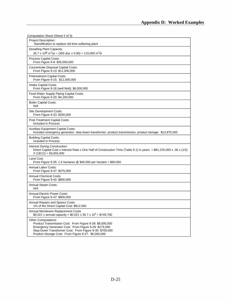
Appendix D: Worked Examples
D-25
Computation Sheet (Sheet 2 of 3) Project Description: Nanofiltration to replace old lime-softening plant
Desalting Plant Capacity: 35.7 x 10⁶ m3/yr ÷ (365 d/yr x 0.90) = 115,000 m3/d
Process Capital Costs: From Figure 9-8: $35,000,000
Concentrate Disposal Capital Costs: From Figure 9-13: $11,000,000
Pretreatment Capital Costs: From Figure 9-15: $11,000,000
Intake Capital Costs: From Figure 9-18 (well field): $6,000,000
Feed Water Supply Piping Capital Costs: From Figure 9-20: $4,100,000
Boiler Capital Costs: N/A
Site Development Costs: From Figure 9-23: $250,000
Post-Treatment Capital Costs: Included in Process
Auxiliary Equipment Capital Costs: Includes emergency generator, step-down transformer, product transmission, product storage: $13,875,000
Building Capital Costs: Included in Process
Interest During Construction: Direct Capital Cost x Interest Rate x One Half of Construction Time (Table 9.1) in years = $81,225,000 x .06 x (1/2) X (18/12) = $3,655,000
Land Cost: From Figure 9-35: 1.5 hectares @ $40,000 per hectare = $60,000
Annual Labor Costs: From Figure 9-37: $375,000
Annual Chemical Costs: From Figure 9-42: $800,000
Annual Steam Costs: N/A
Annual Electric Power Costs: From Figure 9-47: $800,000
Annual Repairs and Spares Costs: 1% of the Direct Capital Cost: $812,000
Annual Membrane Replacement Costs $0.021 x annual capacity = $0.021 x 35.7 x 106 = $749,700
Other Computations: Product Transmission Cost: From Figure 9-28: $8,000,000 Emergency Generator Cost: From Figure 9-29: $175,000 Step-Down Transformer Cost: From Figure 9-30: $700,000 Product Storage Cost: From Figure 9-27: $5,000,000

Desalting Handbook for Planners
D-26
Cost Summary (Sheet 3 of 3) Project Description: Water for the City of Yellowater
Desalting Plant - Type: Nanofiltration Capacity (m3/d): 115,000
Annual Plant Factor (percent): 90 Interest Rate (percent): 6
Annual Production (m3): 35.7 x 10⁶ Plant Life (years): 20
Capital Recovery Factor: 0.0872
CAPITAL COSTS
Capital Cost Centers Est. Cost ($) 1. Desalting Plant 35,000,000
2. Concentrate Disposal 11,000,000
3. Pretreatment 11,000,000
4. Water Intake 6,000,000
5. Feed Water Pipes 4,100,000
6. Steam Supply N/A
7. General Site Development 250,000
8. Post-Treatment Inc. in Plant
9. Auxiliary Equipment 13,875,000
10. Building and Structures Inc. in Plant
Subtotal Direct Capital Cost (DCC) 81,225,000
11. Freight and Insurance 5 percent of DCC 4,061,000
12. Interest During Construction (DCC x Interest Rate x One Half of Construction Time (Table 9.1) in years ) 3,655,000
13. Construction Overhead 15 percent of DCC x factor from figure 9-33 (.95) 11,575,000
14. Owner’s Direct Expense 10 percent of DCC x factor from figure 9-33 (.90) 7,310,000
15. Contingency 10 percent of DCC 8,123,000
Total - Depreciating Capital 115,949,000
16. Land Costs 60,000
17. Working Capital (1/6 x items 18-23) 561,000
Total - Nondepreciating Capital 621,000
Total Capital Costs 116,570,000
ANNUAL COSTS
Annual Cost Centers Est. Cost ($/yr)
18. Operation and Maintenance Labor 375,000
19. Chemicals 800,000
20. Steam N/A
21. Electric Power 800,000
22. Repairs and Spares 812,000
23. Insurance 580,000
Total Operation and Maintenance 3,367,000
24. Annual Costs - Depreciating Capital [(Total-Depreciating Capital – Total Membrane Replacement Cost (i.e. 7 x 749,700)) x 0.0872]
9,653,000
25. Annual Costs - Nondepreciating Capital (Total- Nondepreciating Capital x 0.0872) 54,000
Total Annual Capital Charges 9,707,000
26. Annual Membrane Replacement Costs 749,700
Total Annual Costs (Total O & M and Capital Charges) 13,824,000
COST OF WATER (Total Annual Costs/ Yearly Production) $0.39/m3

Appendix D: Worked Examples
D-27
D-6 Brackish Surface Water EDR
The Dry Creek Municipal Water District takes its water from a brackish creek that flows through the service district. The local Economic Development Agency has been successful in attracting a major government agency facility. However, one of the conditions of locating in the area is that the water supply must meet all Federal and State primary and secondary drinking water standards, including total dissolved solids less than 500 milligrams per liter and chloride less than 250 milligrams per liter. The City needs about 10,000 m3 per day of treated water. A treatability study has shown that because of high silica in the brackish water supply, EDR is the most appropriate treatment technology. The water source is approximately 1000 m from the treatment facility, and has a TDS of about 3000 mg/l. Product water will be transported to an existing storage site approximately 3,500 m away. The land cost in the area is $25,000 per hectare. Concentrate will be sent to 30 hectares of evaporation ponds, requiring a 1,400-meter pipeline.
Note: Amortization is 20 years at 6 percent; annual insurance cost is 0.5% of total capital costs

Desalting Handbook for Planners
D-28
Design Criteria
Item Requirement
Finished water quantity, m3/d (mgd) 10,000 (2.68)
Process capacity, m3/d (mgd) 10,000 (2.68)
Product water quality (mg/l) <500mg/l TDS, <250mg/l Cl
Finished water quality (mg/l) Same
Distance to supply (m) N/A
Number of trains 2
Design feed water temperature (oC) 25
Finished water quality goals: - Total hardness (as CaCO3) - Alkalinity (as CaCO3) - Langelier index
Pump types and sizes: Intake or well pumps Feed pumps (2) Transfer pumps (2) Housekeeping pumps (Cleaning, flushing, etc.) Product pumps High service pumps
N/A Horizontal split case, 521 m3/hr Horizontal split case, 417 m3 /hr N/A N/A N/A
Pretreatment method Existing treatment plant
Post-treatment method pH adjustment, corr. inh., chlorine
Fresh water flush system type N/A
Concentrate disposal method Evaporation ponds
Product storage tank size None
Staffing requirements Table 9-3 - 8 persons
Daily operational period 24 hours
Disinfection equipment type Gas chlorination

Appendix D: Worked Examples
D-29
Economic Criteria Item Requirement
Cost year 2002
Interest rate (%) 6
Service life (yrs) 20
Plant factor (%) 95
Electricity cost ($/kWh) 0.06
Steam cost $/MJ ($/Btu) N/A
Labor rate ($/yr) 25,000
Labor overhead rate (%) Inc.
Contingency (%) 10%
Contractor overhead and labor (%) 15%
Engineering and administration (%) 10%
Freight and insurance (%) 5%
Chemical costs ($/T): Acid Scale inhibitor Caustic Chlorine Sodium bisulfite Anti-foam Lime Coagulant Other
See Table 9-4
Membrane replacement, & stack spares $0.039/m3 based on 10% replacement per year
Repair and spare parts (%/yr) 1%
Facility insurance (%/yr) 0.5%
Land cost ($/hectare) 25,000

Desalting Handbook for Planners
D-30
Supporting Sheet (Sheet 1 of 3)
Project: DCMWD Date: 10/2002
Project Description: Desalting addition to existing brackish surface water treatment
Project Type: EDR
PRODUCT WATER CHARACTERISTICS Annual Requirement: 3.5 x 10⁶ m3 Required Quality: <500 mg/l TDS Distance, Point of Delivery from Desalting Plant: Adjacent
Required Reliability: 95%
Facilities Required: Treatment equipment, building, concentrate pipe, evaporation ponds, land, post-treatment
WATER SUPPLY CHARACTERISTICS Physical Description: Brackish surface water, high silica, acceptable turbidity, and SDI
Chemical Description: Na, 420 mg/l; Ca, 60 mg/l; Mg, 10 mg/l; HCO3, 200 mg/l; Cl, 500 mg/l; SO4, 229 mg/l.
Other: Silica – 72 mg/l
Facilities Required: Feed pumps from existing plant
DESALTING COMPLEX CHARACTERISTICS Process Being Considered: EDR Replaceable Items: Membranes and stack parts Frequency of Replacement (yrs): 10 years Concentrate Disposal Requirements: Evaporation ponds
Service Required at Source: 480V 3ph 60 cycle electrical power
Cost of Services Purchased: Fuel: Steam: Electric Power: $0.06/kWh
Auxiliary Facilities Required: Step-down transformer, emergency generator, product transmission

Appendix D: Worked Examples
D-31
Computation Sheet (Sheet 2 of 3) Project Description: Desalting addition to existing brackish surface water treatment
Desalting Plant Capacity: 3.5 x 10⁶ m3/yr ÷ (365 d/yr x 0.95) = 10,000 m3/d
Process Capital Costs: From Figure 9-9, $8,100,000
Concentrate Disposal Capital Costs: Includes evaporation ponds, concentrate disposal pipeline: $2,330,000
Pretreatment Capital Costs: From Figure 9-15, $1,500,000
Intake Capital Costs: From Figure 9-17, $600,000
Feed Water Supply Piping Capital Costs: From Figure 9-20, $1,000,000
Boiler Capital Costs: N/A
Site Development Costs: From Figure 9-22, $65,000
Post-Treatment Capital Costs: Included in Process
Auxiliary Equipment Capital Costs: Includes product transmission, step-down transformer, emergency generator: $1,425,000
Building Capital Costs: Included in Process
Interest During Construction: Direct Capital Cost x Interest Rate x One Half of Construction Time (Table 9.1) in years = $15,020,000 x .06 x (1/2) x 1 = $451,000
Land Cost: From Figure 9-34, 30.2 hectares x $25000 / hectare = $755,000
Annual Labor Costs: From Figure 9-37, $210,000
Annual Chemical Costs: From Figure 9-41, $180,000
Annual Steam Costs: N/A
Annual Electric Power Costs: From Figure 9-47, $280,000
Annual Repairs and Spares Costs: 1% of the Direct Capital Cost = $150,000
Annual Membrane Replacement Costs: $0.039 x annual capacity = $0.039 x 3.5 x 106 = $136,500
Other Computations: Evaporation Pond Cost, From Figure 9-12: $2,200,000 Concentrate Pipeline Cost, From Figure 9-11: $130,000 Emergency Generator Cost: From Figure 9-29: $25,000 Step-down Transformer Cost: From Figure 9-30: $200,000 Product Transmission Cost: From Figure 9-28: $1,200,000

Desalting Handbook for Planners
D-32
Cost Summary (Sheet 3 of 3) Project Description: Water for the Dry Creek Municipal Water District
Desalting Plant - Type: EDR Capacity (m3/d): 10,000
Annual Plant Factor (percent): 95 Interest Rate (percent): 6
Annual Production (m3): 3.5 x 10⁶ Plant Life (years): 20
Capital Recovery Factor: 0.0872
CAPITAL COSTS
Capital Cost Centers Est. Cost ($) 1. Desalting Plant 8,100,000
2. Concentrate Disposal 2,330,000
3. Pretreatment 1,500,000
4. Water Intake 600,000
5. Feed Water Pipes 1,000,000
6. Steam Supply N/A
7. General Site Development 65,000
8. Post-Treatment Inc. in Plant
9. Auxiliary Equipment (Step down transformer, product transmission) 1,425,000
10. Building and Structures Inc. in Plant
Subtotal Direct Capital Cost (DCC) 15,020,000
11. Freight and Insurance 5 percent of DCC 751,000
12. Interest During Construction (DCC x Interest Rate x One Half of Construction Time (Table 9.1) in years ) 451,000
13. Construction Overhead 15 percent of DCC x factor from figure 9-33 (1.01) 2,278,000
14. Owner’s Direct Expense 10 percent of DCC x factor from figure 9-33 (1.07) 1,607,000
15. Contingency 10 percent of DCC 1,502,000
Total - Depreciating Capital 21,609,000
16. Land Costs 755,000
17. Working Capital (1/6 x items 18-24) 155,000
Total - Nondepreciating Capital 910,000
Total Capital Costs 22,519,000
ANNUAL COSTS
Annual Cost Centers Est. Cost ($/yr)
18. Operation and Maintenance Labor 210,000
19. Chemicals 180,000
20. Steam N/A
21. Electric Power 280,000
22. Repairs and Spares 150,000
23. Insurance 108,000
Total Operation and Maintenance 928,000
24. Annual Costs - Depreciating Capital [(Total-Depreciating Capital – Total Membrane Replacement Cost (i.e. 10 x 136,500)) x 0.0872])
1,765,000
25. Annual Costs - Nondepreciating Capital (Total- Nondepreciating Capital x 0.0872) 79,000
Total Annual Capital Charges 1,844,000
26. Annual Membrane Replacement Costs 136,500
Total Annual Costs (Total O & M and Capital Charges) 2,909,000
COST OF WATER (Total Annual Costs/ Yearly Production) $0.83/m3

Appendix E: Glossary
E-1
Appendix E: Glossary
AC – Alternating electrical current. ACIDIFICATION – The addition of acid to the feed water of a desalting plant, usually to prevent alkaline calcium carbonate and magnesium hydroxide scale. ALKALINE – Water containing sufficient amounts of alkalinity to raise the solution pH above 7.0. ALKALINITY – The ability of water to neutralize an acid because of the presence of bicarbonate, carbonate, and hydroxyl ions. AMBIENT TEMPERATURE – Temperature of surroundings, usually assumed to be 20-25 oC. ANION – An ion carrying a negative charge. In an electrolytic cell, it migrates toward the anode. ANODE – The positive electrode of an electrodialysis cell. ANNUAL COST – The total yearly cost of owning and operating a desalting plant. This cost includes carrying charges on the investment, taxes, insurance, interest on working capital, operating and maintenance labor, energy costs, consumable supplies, repair and replacement costs, and the cost of concentrate disposal. ANTISCALANT – See Scale Inhibitor. ATOM – The smallest particle of an element possessing all the chemical characteristics of that element. BACK PRESSURE VALVE – A valve placed in a piping system to restrict the fluid flow, thus pressurizing the system. The valve is usually spring- or gas-pressure loaded so that any desired system pressure may be present. BACKWASH – Reversed flow in a filter, ion-exchange column, or membrane filter to remove or wash away accumulated suspended materials. BACTERIA – Microscopic organisms, usually consisting of a single cell. BAR – Unit of pressure. 1 bar = 14.5 lb/in2. BASIC SOLUTION – Solution containing an excess of hydroxyl ions and with a pH greater than 7.0.

Desalting Handbook for Planners
E-2
BLENDING – Mixing waters of different purity and constituents to form a diluted solution. BLOWDOWN – See Concentrate Reject (Stream). BOILING POINT ELEVATION (BPE) – The difference between the boiling point of a solution and the boiling point of pure water at the same elevation. BRACKISH WATER – Saline water with a salt concentration ranging from 1,000 mg/l to about 25,000 mg/l total dissolved solids (TDS). BTU – British thermal unit. The quantity of heat required to increase the temperature of 1 pound of water 1 oF. CAPITAL COST – Total capital cost includes the indirect costs associated with owner’s costs of studies, engineering, licenses, interest on working capital, and insurance during the construction period, as well as the direct capital costs. It is the owner’s total investment up to the point that the plant is put into useful operation. CATHODE – Negative electrode of an electrodialysis cell. CATION – The ion in an electrolytic solution that migrates to the cathode. It carries a positive charge. CHANNELING – Unevenly distributed flow that may occur, for example, in a sand filter, an electrodialysis cell, or in a reverse osmosis membrane. CHEMICAL CLEANING – All-inclusive term for any of a number of in situ chemical cleaning techniques to remove fouling and scale from membranes and thermal heat transfer surfaces. CHEMICAL EQUATION – Notation used to describe how atoms combine to form molecules. CHEMICAL EQUILIBRIUM – When chemical reactions occur, not all of the reactants react to form products. The solution attains a chemical equilibrium. At equilibrium, there may be residual reactants or products. CHEMICAL FORMULA – Notation used to describe molecules (e.g., the formula for water is H2O). CHEMICAL REACTION – Phenomena when atoms unite, separate, or exchange places in the ratio of their particular atomic weights or simple multiples thereof. COAGULATION – The precipitation of substances in colloidal solution. COMPOUND – A substance that can be decomposed by chemical processes into two or more elements or which can be built up from two or more elements (e.g., sodium chloride, NaCl).

Appendix E: Glossary
E-3
CONCENTRATE – The concentrated wastewater flow from reverse osmosis, electrodialysis, and nanofiltration plants. CONCENTRATE REJECT (STREAM) – The concentrated wastewater flow from a desalting plant, containing most of the salts from the original feed water. Also referred to as blowdown. CONCENTRATE SATURATION PRESSURE – The pressure corresponding to the concentrate stream temperature at which boiling occurs. CONCENTRATION POLARIZATION – The concentration or depletion of salt ions at membrane surfaces. CONCENTRATION RATIO – The salinity of the concentrate divided by the salinity of the plant feed water. CONDENSATE – Distilled water formed by cooling and condensing water vapor. CONDENSER TUBES – Tubes used to heat or reheat concentrate in the distillation process while simultaneously condensing water vapor. CONDUCTIVITY – See Specific Conductance. CONJUNCTIVE USE – A desalting plant operating on a part-time basis to supplement a water supply. CONTAMINANT – Any undesirable substance in a water source. DC – Direct electrical current. DEAERATION – A process to remove oxygen and other noncondensable gases from the feed water stream. DECARBONATION – A process to remove carbonate alkalinity from the feed water as CO2 gas. DEMINERALIZATION – Any process that removes mineral substances from water. DESALINATION – Process of removing salts from water sources. DIFFERENTIAL WATER COST – In this report, the deviation from a selected water cost basis as the result of changes in various operating conditions. DIRECT CONTACT HEAT EXCHANGE – The process in which a liquid, gas, or solid to be heated or cooled is brought into direct contact with the heating or cooling medium.

Desalting Handbook for Planners
E-4
DISSOLVED SUBSTANCE – A substance that has gone into solution in water. See Solution. DISTILLATE – The final product water from a distillation plant. DISTILLATION – A method of desalting water that uses heat to vaporize water and to collect the condensed water. DISTRIBUTION SYSTEM – The pipes, conduits, and canals bringing water to the consumers. DIVALENT ION – An ion carrying a double charge, either positive or negative. Example: Mg+2, SO-4. DUAL-PURPOSE PLANT – A plant that produces both electric power and desalted water. EFFECT – A single evaporation or single step in a multi-effect evaporator arrangement. EFFLUENT – Water leaving a desalting process. May be applied to both concentrate or product water. ELECTROCHEMISTRY – Science dealing with the relation of electricity to chemical changes. ELECTRODIALYSIS (ED) – A process by which ions are transferred through membranes to a more concentrated solution as a result of using a direct current electrical potential. ELECTRODIALYSIS REVERSAL (EDR) – A variation of ED in which polarity and cell function change periodically to maintain efficient performance. ELECTROLYTE – A compound that disassociates into ions when dissolved in water. ELEMENT – A simple substance that cannot be decomposed by chemical processes into simpler substances (e.g., chlorine, hydrogen, oxygen, sodium). ENERGY RECOVERY – Possible energy saving in reverse osmosis in which the concentrate stream, under pressure, is used to drive a turbine that provides part of the feed pressure requirement. ENTHALPY – A measure of the total energy content of a material or system. ENTRAINMENT SEPARATOR – A device for separating entrained water droplets from the vapor produced in a distillation plant. EQUIVALENT PER MILLION – Calculated by dividing the concentration in parts per million by the equivalent weight.

Appendix E: Glossary
E-5
EQUIVALENT WEIGHT – The weight of an ion determined by the sum of the component weight of its atoms by its valence. EVAPORATION – The process by which water is converted to a vapor that can be condensed. EVAPORATOR – A process device in which water is boiled and the water vapor is collected and condensed to form a distilled product water. EXPRESSED AS CALCIUM CARBONATE (CaCO3) – Indicates that the reported quantity of a compound has been converted to an equivalent quantity of CaCO3. FEED-TO-PRODUCT CONCENTRATION RATIO – Product concentration divided by the feed concentration. Often expressed as percent. Sometimes referred to as “cut” in the electrodialysis process. FEED WATER – Saline water supplied to the desalting plant for processing. FIXED CHARGES – Charges associated with the operation of a desalting plant that continue to accrue, whether the plant is operating or not. This cost includes interest, amortization, taxes, and insurance. FLASHING – A physical process in which a preheated water encounters a reduced pressure that causes part of the water to boil rapidly or flash into steam. FLASHING THERMAL POTENTIAL – When a water under sufficient pressure is raised to a temperature higher than the saturation temperature corresponding to a subsequent system pressure, the water is said to have “flashing thermal potential.” FLOCCULATION – The gathering together of small particles in water after adding coagulant chemicals. FLUTED SURFACE TUBES; FINNED TUBES – Tubes of an evaporator or condenser in which the heat transfer rate is enhanced by a series of corrugations or ridges and valleys running parallel to or spiraling along the length of the tube. FLUX – Term used in reverse osmosis to indicate the rate of water permeation through the membrane. Usually expressed as gallons per square foot per day in the U.S., and liters per square meter per hour in metric. FOULING – The reduction in performance of process equipment (heat transfer tubing, membranes, etc.) that occurs as a result of scale buildup, biological growth, or the deposition of colloidal material.

Desalting Handbook for Planners
E-6
GENERAL AND ADMINISTRATIVE COSTS – An expense usually calculated as a percent of labor cost plus payroll additives to cover the costs associated with timekeeping, payroll, overhead, and administration. GROUND WATER – Water normally found underground and obtained from wells. HARDNESS – Usually measured in CaCO3. “Hardness” in water is the sum of calcium and magnesium concentrations, both expressed as calcium carbonate, CaCO3, in milligrams per liter. These constituents cause soaps to precipitate. HEAT EXCHANGER – An apparatus in which heat is transferred from one medium to another. HEAT OF VAPORIZATION – The quantity of heat required to vaporize 1 unit of liquid to 1 unit of dry vapor. For water at one atmosphere, approximately 1,000 Btu/lb or 2.32 MJ/kg. HEAT RECOVERY SECTION – The portion of a flash distillation evaporator where the feed stream recovers heat from condensing vapors. HEAT REJECTION SECTION – The portion of a flash distillation evaporator where the heat released by the condensing vapors is rejected to waste with the condenser cooling water. HEAT TRANSFER – Physical phenomenon dealing with the flow of heat. The subject is particularly important in the distillation and freezing processes in which heat is transferred from medium to medium, usually through a heat transfer surface. HEAT TRANSFER COEFFICIENT – An engineering design factor defining the heat transfer rate in a heat exchanger. Usually given in terms of Btu/hr-ft2-oF temperature difference. HYBRID PLANTS – Plants that combine two or more processes. HYDROLYSIS – A chemical process of decomposition involving splitting of a bond and addition of the ions of water. HYDROXYL ION – The (OH-) ion present in water. IMMISCIBLE LIQUIDS – Liquids incapable of mixing or attaining homogeneity. INDIRECT CAPITAL COSTS – The owner’s costs associated with such items as studies, planning, engineering, construction supervision, licensing, startup, public relations, and training. These costs are a part of the cost of placing the plant in operation and are in addition to the direct capital costs associated with equipment and contracts for construction. INORGANIC – Substances of mineral origin, such as sand, salt, iron, and calcium salts. INSOLUBLE MATERIALS – Materials that do not dissolve, or dissolve only slightly, in water.

Appendix E: Glossary
E-7
INTAKE EQUIPMENT – The works or structures at the head of a conduit into which the feed water entering the desalting plant is directed. INVERSE SOLUBILITY – The characteristic attributed to a substance that becomes less soluble with increasing temperature (e.g., calcium carbonate). ION – An atom or group of atoms that carries a positive or negative electric charge as a result of having lost or gained one or more electrons. An electrically charged atom, radical, or molecule formed by the loss or gain of electrons. IONIZABLE – Compounds, such as salts, that form ions when dissolved in water. These materials lend themselves to separation by electrodialysis. Many organic materials are not ionizable, and separation can only be accomplished by physical processes such as reverse osmosis or distillation. See also Electrolyte. KWH – Kilowatthours. A measure of electrical usage. LANGELIER SATURATION INDEX – Measure of a water’s corrosion or scale-forming tendencies. LATENT HEAT – The amount of heat required to cause a change of state without temperature change, as in the melting of ice (latent heat of fusion) or the evaporation of water (latent heat of evaporation). See Heat of Vaporization. MEMBRANE – In desalting, used to describe a semipermeable film. Membranes used in electrodialysis are permeable to ions of either positive or negative charge. Reverse osmosis and nanofiltration membranes ideally allow the passage of pure water and block the passage of salts. MICROMHO – A unit measure of conductivity equal to one millionth of a mho. Mho is the reciprocal of ohm. MICROFILTRATION – A membrane used to treat water, with a 0.05 - 5 micron pore size. The membrane filters out turbidity, algae, Giarda and Cryptosporidium spores, and bacteria. The membrane operates by sieving. MICRON – A unit of length equal to one thousandth of a millimeter. MICROORGANISM – A plant or animal of microscopic size. MINERAL REDUCTION – Partial removal of dissolved salts from water.

Desalting Handbook for Planners
E-8
MODULE – The smallest packaged functional assembly of a desalting plant. A section or integral portion of a desalting plant that is used initially to study large-scale technology and critical design features in preparation for subsequent prototype construction. MOLE – The quantity of a chemical substance measured in mass units (e.g., grams or pounds) that are numerically equal to the molecular weight. For a gas, the volume occupied by such a weight under specified conditions. MOLECULE – The smallest quantity of a compound that possesses all the chemical characteristics of that compound. MONOVALENT ION – An ion that carries only a single charge, either positive or negative. Example: Na+, Cl-. NANOFILTRATION – A membrane used to desalinate water. The membrane has a molecular weight cutoff of about 100, and rejects ions with greater than 100 molecular weight at about 90 percent. The membrane operates by overcoming osmotic pressure. NONCONDENSABLE GASES – Gases such as air and carbon dioxide that do not condense to liquid with the water vapor when heat is removed. NONELECTROLYTE – See Electrolyte. ORGANIC – Substances that come from plant or animal sources and always contain carbon. ORGANIC COMPOUND – A compound in which the major elements are carbon and hydrogen. OSMOSIS – Movement of water from a dilute solution to a more concentrated solution through a membrane separating the two solutions. See Reverse Osmosis. OSMOTIC PRESSURE – The potential energy difference between two solutions of different concentrations separated by a permeable membrane. OXIDATION – The addition of oxygen, removal of hydrogen, or removal of electrons from an element or compound. PATHOGENS – Disease-causing organisms. PERFORMANCE RATIO (PR) – A performance rating associated with the distillation desalting process. It is defined as the number of pounds of distillate produced for each 1,000 Btu of heat input, or as kg/MJ in metric. PERMANENT HARDNESS – That part of the hardness that cannot be removed by boiling. Also known as noncarbonate hardness.

Appendix E: Glossary
E-9
PERMEATE – The product water from a desalting process (also called product). pH – A number indicating the hydrogen-ion concentration in a solution. Values greater than 7.0 indicate a basic (alkaline) solution; values less than 7.0 indicate an acidic solution. PILOT PLANT – An experimental unit of small size, usually less than 400 m3/d (0.1 mgd) capacity, used for early evaluation and development of new, improved processes and to obtain technical and engineering data. PLANT LOAD FACTOR – Also known as “Plant Factor” or “Load Factor.” The fraction, or percentage, of full-scale annual design capacity that is actually produced by a desalting plant. POLYAMIDE – A polymer formed by polymerization of an ester. POLYMER – A chemical compound formed by polymerization. POLYMERIZATION – A chemical reaction in which smaller molecules of the same kind (or sometimes of two or three different kinds) combine to form larger molecules. POST-TREATMENT – The processes, such as pH adjustment and chlorination, that may be employed on the product water from a desalting unit. POTABLE WATER – Water that does not contain objectionable pollution, contamination minerals, or infective agents and is considered suitable for drinking. In desalting, potable water is typically defined as having a salinity less than 500 ppm TDS (USPHS – Drinking Water Standards, 1962) and to be in compliance with Federal and State regulations. PRECIPITATE – A substance separated from a solution by chemical or physical change as an insoluble amorphous or crystalline solid. PRETREATMENT – The processes such as chlorination, clarification, coagulation, scale inhibition, acidification, and deaeration that may be employed on the feed water to a desalting unit to minimize algae growth, scaling, and corrosion. PRODUCT – The final desalted water, called “distillate” in distillation, “dilute” in electrodialysis, and “product” in the reverse osmosis and nanofiltration processes. PRODUCT – In a chemical equation, the result of the chemical reaction. Noted on the right side of the equation. PROTOTYPE – A full-size, first-of-kind production plant used for development, study, and demonstration of full-sized technology, plant operation, and process economics. REACTANT – A chemically reacting substance. Item on the left side of a chemical equation.

Desalting Handbook for Planners
E-10
RECOVERY RATIO – The ratio of the product flow rate to the feed water flow rate. This ratio is sometimes called the conversion ratio. RECURRING COSTS – Plant fixed costs associated with annual tax and insurance costs. REPLACEABLE ITEMS – Plant equipment with an estimated life less than the useful plant lifetime or the plant design lifetime. REVERSE OSMOSIS (RO) – Method of desalination which uses pressure to move water from a concentrated solution to a dilute solution through a membrane separating the two solutions. See Osmosis. SALINE WATER – Water with dissolved solids exceeding the limits of potability. Saline water may include sea water, brackish water, mineralized ground and surface water, and irrigation return flows. SALT DIFFUSION – The movement of ions or molecules under influence of a concentration difference. SALT REJECTION – A factor expressing the ability of RO membranes to reject dissolved solids. Usually given as: feed concentration minus product concentration divided by feed concentration, and expressed as percent. SALT TRANSPORT – Salt that transfers through reverse osmosis membranes, along with water. SATURATED SOLUTION – A solution that contains the maximum amount of solute that can be dissolved at equilibrium. See Solubility. SATURATION TEMPERATURE – The temperature of a liquid, under a given pressure, at which boiling and condensing occur. SCALE – Salts deposited on heat transfer or membrane surfaces that retard the rate of heat transfer or ion or water permeation. SCALE INHIBITOR – An agent that ties up and, thus, inactivates certain metal ions. It may be added to a feed water to extend the limits of saturation of scaling substances. The sequestering of calcium ions to prevent calcium sulfate precipitation is an example. Also known as antiscalant, sequestering agent. SECONDARY SEWAGE EFFLUENT – Sewage that has been processed through the conventional primary and secondary treatment stages. SEMIPERMEABLE MEMBRANE – A membrane that is permeable for certain molecules or ions only. RO membranes, for example, ideally will pass water but not salt. ED membranes pass ions with a certain charge but not water.

Appendix E: Glossary
E-11
SHELL – The vessel that contains the heat exchanger or condenser tubing. SOFT WATER – A water that has a minimal amount of calcium and magnesium ions. Such waters frequently contain substantial amounts of sodium. SOLUBILITY – A measure of the maximum amount of a certain substance that can dissolve in a given amount of water, or other solvent, at a given temperature. SOLUTE – A dissolved substance. SOLUTION – A homogeneous mixture of substances in which the molecules of the solute are uniformly distributed among the molecules of the solvent, such as water. SPECIFIC CONDUCTANCE (CONDUCTIVITY) – Quantitative expression for the capability of a particular solution to conduct electricity. It is defined as the conductance of a cube of that particular water that is 1 cm long and has a cross sectional area of 1 cm2. Conductivity is usually expressed in micromohos per centimeter. SPECIFIC GRAVITY – The ratio of the density of a substance to the density of water at specific temperatures. SPECIFIC POWER – Desalting plant power or energy consumption evaluated as a function of water production. Usually given in kWh per 1,000 gallons or kWh per cubic meter. STACK – The alternating array of cation and anion permeable membranes, spacers, gaskets, and electrodes used in the electrodialysis desalting process. STAGE – A unit of desalting equipment capable of purification and separation of the feed water into product and concentrate. If separation is insufficient, more than one stage can be arranged in series. SUPERSATURATED SOLUTION – A solution containing more solute than its normal solubility would allow. This is a nonequilibrium and, therefore, temporary situation. The solute has a strong tendency to come out of solution as crystals until the saturated condition has been reached. SURFACE WATER – Water above the water table. SUSPENDED SUBSTANCE OR SUSPENDED SOLIDS – Materials that are not dissolved but are in suspension in the form of finely divided particles. Suspended materials may be removed by physical means such as filtration. TEMPORARY HARDNESS – Hardness that can be removed by boiling.

Desalting Handbook for Planners
E-12
THERMODYNAMIC EQUILIBRIUM – A condition in which the temperature of a liquid is in balance with its vapor pressure such that no boiling or condensing is occurring. THERMODYNAMICS – A science dealing with the mechanical action or relations of heat. TITRATION – Chemical method of determining the strength of a solution by measuring the volume of a reacting standard solution of known concentration. TUBE BUNDLE – A series of tubes compactly arranged in an evaporator shell to provide the required heat transfer surface. TUBE SHEET – The end plate in a tube bundle to which all of the tubes are attached. TUBING – Typically, flexible piping of small diameter, generally less than 5 centimeters (approximately 2 inches), used in distillation processes. TUBING AREA – Surface area of tubing. TURBIDITY – Opaqueness or cloudiness caused by the presence of suspended particles in water, usually stirred-up sediments. The turbidity of a water is measured by its capacity for absorbing or scattering light. TURBINE CYCLE – Use of turbines to generate power from high-pressure steam. Low-pressure effluent steam from such turbines can be used to drive a desalting plant. TURBULENT FLOW – A fluid flow condition in which the velocity at a given point varies erratically in magnitude and direction. ULTRAFILTRATION – A membrane used to treat water with about a 10,000-300,000 molecular weight cutoff. The membrane rejects organic macromolecules, viruses, and asbestos. The membrane operates by sieving. UNIT COST – The cost per unit of product water output ($/1,000 gallons, $/cubic meter) or per unit energy input ($/M Btu, cents/kWh, $/MJ). VALENCE – Number indicating the capacity of an atom to combine with another element. WASTE CONCENTRATE – See Concentrate Reject (Stream). Sometimes called blowdown. WATER CHEMISTRY – A branch of science dealing with the chemical properties of water and its dissolved and suspended constituents. WATER PERMEABILITY – The capacity of a membrane to allow water to pass through. See Flux.

Appendix E: Glossary
E-13
WATER TABLE – The upper limit of the portion of the ground wholly saturated with water. This can be near the ground’s surface or many feet below it. See Surface Water. WATER TRANSPORT – The tendency for water to pass through a membrane. Water transport is desirable in reverse osmosis but undesirable in electrodialysis.

Appendix F: Common Conversions From To Multiply by
Mass & Length Kilograms (Kg) Pounds (lbs) 2.2046 Metric tons (tonnes) US tons (tons) 1.1023 Meters (m) Feet (ft) 3.2808 Centimeters (cm) Inches (in) 0.3937 Millimeters (mm) Inches (in) 0.0394
Area Square meters (m2) Square feet (ft2) 10.7639 Square centimeters (cm2) Square inches (in2) 0.155 Hectares Acres 2.4711
Volume Cubic meters (m3) Gallons (g) 264.1721 Cubic meters (m3) Liters (l) 1000 Cubic meters (m3) Acre-feet 8.11E-04 Cubic meters/day (m3/d) Million gallons/day (mgd) 2.64E-04 Cubic meters/hour (m3/hr) Gallons/minute (gpm) 4.4029 Cubic meters (m3) Thousand gallons (kgal) 0.2642 Liters per minute (lpm) Gallons per minute (gpm) 0.2642 Liters per square meter per hour (l/m2/hr) Gallons per square foot per minute 4.09E-04 Liters per square meter per hour (l/m2/hr) Gallons per square foot per hour 0.0245 Liters per square meter per hour (l/m2/hr) Gallons per square foot per day 0.589
Pressure Bars Pounds/square inch (psi) 14.5038 Bars Kilograms/sq. centimeter (Kg/cm2) 1.0197 Kilograms/sq. centimeter (Kg/cm2) Pounds/square inch (psi) 14.2233 Kilopascals (kPa) Pounds/square inch (psi) 0.145
Energy & Heat Transfer Joules (J) British thermal units (Btu) 9.49E-04 Joules/gram Btu/pound 0.4299 Joules/gram degree C Btu/lb degree F 0.2388 Calories/gram degree C Btu/lb degree F 1 Kilowatts (kW) Btu/hr 3414.43 Kilowatt-hours (kWh) Btu 3412.76 Kilowatt-hours/cubic meter Kilowatt-hours/thousand gallons 3.7854 (kWh/m3) (kWh/kgal) Micro ohms/cm Micro ohms/in 2.54 Micromhos/cm Micromhos/in 2.54 Watts/sq. meter degree K (W/m2-K) Watts/sq. feet degree K (W/ft2-K) 0.0929 ohms/sq. centimeters ohms/sq. inches 6.4516 Mega joules (MJ) Btu 947.8171 Mega joules (MJ) Thousand Btu (kBtu) 0.9478 Mega joules per cubic meter (MJ/m3) Btu per gallon (Btu/gal) 3.5879
F-1