DERIVED CATEGORIES OF TWISTED SHEAVES ON

CALABI-YAU MANIFOLDS

A Dissertation

Presented to the Faculty of the Graduate School

of Cornell University

in Partial Fulfillment of the Requirements for the Degree of

Doctor of Philosophy

by

Andrei Horia Caldararu

May 2000

c© 2000 Andrei Horia CaldararuALL RIGHTS RESERVED

DERIVED CATEGORIES OF TWISTED SHEAVES ON CALABI-YAUMANIFOLDS

Andrei Horia Caldararu, Ph.D.Cornell University 2000

This dissertation is primarily concerned with the study of derived categories oftwisted sheaves on Calabi-Yau manifolds. Twisted sheaves occur naturally in avariety of problems, but the most important situation where they are relevantis in the study of moduli problems of semistable sheaves on varieties. Althoughuniversal sheaves may not exist as such, in many cases one can construct themas twisted universal sheaves. In fact, the twisting is an intrinsic property of themoduli problem under consideration.

A fundamental construction due to Mukai associates to a universal sheaf atransform between the derived category of the original space and the derived cat-egory of the moduli space, which often turns out to be an equivalence. In thepresent work we study what happens when the universal sheaf is replaced by atwisted one. Under these circumstances we obtain a transform between the de-rived category of sheaves on the original space and the derived category of twistedsheaves on the moduli space.

The dissertation is divided into two parts. The first part presents the maintechnical tools: the Brauer group, twisted sheaves and their derived category, aswell as a criterion for checking whether an integral transform is an equivalence(a so-called Fourier-Mukai transform). When this is the case we also obtain re-sults regarding the cohomological transforms associated to the ones on the level ofderived categories.

In the second part we apply the theoretical results of the first part to a largeset of relevant examples. We study smooth elliptic fibrations and the relationshipbetween the theory of twisted sheaves and Ogg-Shafarevich theory, K3 surfaces,and elliptic Calabi-Yau threefolds. In particular, the study of elliptic Calabi-Yauthreefolds leads us to an example which is likely to provide a counterexample to thegeneralization of the Torelli theorem from K3 surfaces to threefolds. A similaritybetween the examples we study and certain examples considered by Vafa-Wittenand Aspinwall-Morrison shows up, although we can only guess the relationshipbetween these two situations at the moment.

Biographical Sketch

Andrei Caldararu was born in Bucharest, Romania, in 1971. After attending the“Sf. Sava” high-school and one year at the Bucharest University, he moved toJerusalem, Israel. He graduated summa cum laude from the Hebrew University inJerusalem in 1993, with a double degree in Mathematics and Computer Science.After working for a year in the computer industry, he started his work towards aPh.D. in Mathematics at Cornell University. Andrei is married to Daniela, andthey currently live in New York City.

iii

Tuturor celor din care am fost facut, ın spirit si ın lut.

iv

Acknowledgements

This dissertation would not have existed without the continuous effort of my ad-visor, Mark Gross. Taking me from the stage when doing research in mathematicsseemed impossible to the point of writing this finished result required lots of hours,patience, and encouragement, and I want to thank him for this.

Another person whose effort to give me a mathematical education is invaluableis Sorin Popescu, who completed and complemented Mark’s work. Multumesc.

The ragged trajectory of the six years that lead to this dissertation has carriedme in numerous places. Among these I want to particularly thank Cornell (forbeing a true alma mater to me), Warwick, Columbia. The Einaudi Center atCornell provided generous funding for part of my travels to England.

Of course one’s education (mathematical and otherwise) is the result of inter-actions with many more people. Stefan Davidovici, Mirel and Luminita Caibar,Luis O’Shea and David Tang have made my life better during these six years. Theconversations with Titus Teodorescu, Tom Bridgeland, Tony Pantev, and MilesReid have led to many of the ideas in this work.

Last, and first, there is my family. Without my wife, Dana, and without myparents, Monica and Horia, nothing would have been possible. Their contributionwas essential to the existence of this work, and I want to thank them for everything.

And then there are those people whose influence can not be traced directlyto this work, but whose ideas and example pervade everything I do. I cannotoverestimate the influence Florian Colceag and Doru Davidovici have had in mylife. I wish I could be like them.

v

Table of Contents

Introduction and Overview 1

I Theoretical Results 6

1 Twisted Sheaves 71.1 H2

et(X,O∗X), the Brauer Group and Gerbes . . . . . . . . . . . . . . 7

1.2 Twisted Sheaves . . . . . . . . . . . . . . . . . . . . . . . . . . . . . 131.3 Modules over an Azumaya Algebra . . . . . . . . . . . . . . . . . . 18

2 Derived Categories of Twisted Sheaves 262.1 Preliminary Results . . . . . . . . . . . . . . . . . . . . . . . . . . . 262.2 The Derived Category and Derived Functors . . . . . . . . . . . . . 292.3 Relations Among Derived Functors . . . . . . . . . . . . . . . . . . 342.4 Duality for Proper Smooth Morphisms . . . . . . . . . . . . . . . . 37

3 Fourier-Mukai Transforms 383.1 Integral Functors . . . . . . . . . . . . . . . . . . . . . . . . . . . . 383.2 Equivalences of Twisted Derived Categories . . . . . . . . . . . . . 453.3 Moduli Spaces and Universal Sheaves . . . . . . . . . . . . . . . . . 46

II Applications 49

4 Smooth Elliptic Fibrations 504.1 Elliptic Fibrations . . . . . . . . . . . . . . . . . . . . . . . . . . . . 504.2 The Relative Jacobian . . . . . . . . . . . . . . . . . . . . . . . . . 514.3 The Twisted Poincare Bundle . . . . . . . . . . . . . . . . . . . . . 534.4 Ogg-Shafarevich Theory . . . . . . . . . . . . . . . . . . . . . . . . 554.5 Other Fibrations . . . . . . . . . . . . . . . . . . . . . . . . . . . . 57

5 K3 surfaces 625.1 General Facts . . . . . . . . . . . . . . . . . . . . . . . . . . . . . . 635.2 Deformations of Twisted Sheaves . . . . . . . . . . . . . . . . . . . 685.3 Identifying the Obstruction . . . . . . . . . . . . . . . . . . . . . . 735.4 The Map on Brauer Groups . . . . . . . . . . . . . . . . . . . . . . 78

vi

5.5 Relationship to Derived Categories . . . . . . . . . . . . . . . . . . 82

6 Elliptic Calabi-Yau Threefolds 856.1 Generic Elliptic Calabi-Yau Threefolds . . . . . . . . . . . . . . . . 866.2 Examples . . . . . . . . . . . . . . . . . . . . . . . . . . . . . . . . 886.3 Jacobians of Curves of Genus 1 . . . . . . . . . . . . . . . . . . . . 926.4 The Relative Jacobian . . . . . . . . . . . . . . . . . . . . . . . . . 996.5 The Twisted Pseudo-Universal Sheaf and

Derived Equivalences . . . . . . . . . . . . . . . . . . . . . . . . . . 1026.6 Equivalent Twistings . . . . . . . . . . . . . . . . . . . . . . . . . . 1056.7 Applications to the Torelli Problem . . . . . . . . . . . . . . . . . . 1086.8 Relationship to Work of Aspinwall-Morrison and Vafa-Witten . . . 112

III Open Questions and Further Directions 115

Bibliography 117

vii

List of Figures

6.1 The Kahler cones in Example 6.2.2 . . . . . . . . . . . . . . . . . . 906.2 The Kahler cones in Example 6.2.3 . . . . . . . . . . . . . . . . . . 91

viii

Convention

Throughout this work we make the assumption that the ground field is C. Mostof the results hold over an arbitrary field as well, with only minor modifications.

It is also important to be precise about the topology being used. Most of thetime we use the etale topology when working in the algebraic setting, and theEuclidean (analytic) topology in the analytic setting. For details regarding theetale topology the reader should consult [30]; the analytic case is studied in detailin [2].

ix

Introduction and Overview

Twisted sheaves were introduced by Giraud ([16]) as part of his study of non-commutative cohomology, but passed relatively unnoticed in that context and werenot studied as objects of intrinsic interest. The purpose of this dissertation is topresent their theory, with an emphasis on their derived category, and to showthat twisted sheaves provide a powerful and useful tool in the study of algebraicvarieties and complex manifolds.

Informally speaking, a twisted sheaf consists of a collection of sheaves andgluing functions, with the apparent defect that these gluing functions “don’t quitematch up.” In this respect they have a strong similarity with vector bundles on aspace: these are vector spaces and gluing functions that also “don’t quite matchup.” When the gluings match up, for a vector bundle, the result is a trivial vectorbundle (i.e. a vector space). The similar situation for twisted sheaves gives atrivially twisted sheaf, which is a sheaf. In a certain sense, twisted sheaves are thenext level of generalization, up from vector bundles.

Let’s be a little more precise (the full definition of the category of twistedsheaves is given in Section 1.2). Consider a scheme or analytic space X, and anelement α of the Brauer group of X (roughly, this is the same as H2(X,O∗X)).Represent α by a Cech 2-cocycle on some open cover Uii∈I , i.e., find sections

αijk ∈ Γ(Ui ∩ Uj ∩ Uk,O∗X)

that satisfy the coboundary condition and whose image in H2(X,O∗X) is α. Anα-twisted sheaf is then a collection

(Fii∈I , ϕiji,j∈I)

of sheaves and isomorphisms such that Fi is a sheaf on Ui,

ϕij : Fj|Ui∩Uj → Fi|Ui∩Ujis an isomorphism, and these isomorphisms satisfy

ϕij ϕjk ϕki = αijk · idFi

along Ui ∩ Uj ∩ Uk, for any i, j, k ∈ I.It is easy to see that under the natural definitions of homomorphisms, kernel,

cokernel, etc., the α-twisted sheaves form an abelian category. The question is,then, what information about X can we deduce from this category?

1

2

First, this category is invariant of the choices made: it does not depend onthe choice of the open cover, or of the particular Cech cocycle. Moreover, in mostinteresting cases there is another, more natural description of this category, as thecategory of sheaves of modules over a sheaf of non-commutative algebras. In thissense, the category of twisted sheaves should be viewed as a non-commutative ana-logue of the category of coherent sheaves on the underlying scheme or analytic spaceX. However, this non-commutative situation is just a very mild generalization ofthe commutative setting, because the non-commutative algebras that appear inthis way are the simplest possible ones, Azumaya algebras. (For a descriptionof Azumaya algebras, the reader should consult Section 1.1; for the equivalencebetween twisted sheaves and sheaves of modules over an Azumaya algebra, seeSection 1.3.)

The question that arises at this point is, why are twisted sheaves interesting,and where do they occur naturally? A starting point would be the study of Brauer-Severi varieties (Pn-bundles which are not locally trivial in the Zariski topology,but are locally trivial in finer topologies, like the etale or the analytic topology).But the most important occurrence of twisted sheaves is in the study of modulispaces of semistable sheaves on projective varieties.

The difficulty with most moduli problems is that they are not fine: althougha moduli space exists (which parametrizes in a nice, algebraic way the objectsunder consideration), a universal object fails to exist. In the case of semistablesheaves on a projective variety X, this means that a moduli space M exists (whosepoints [F ] correspond to semistable sheaves F on X), but there does not exist auniversal sheaf on X ×M , i.e. a sheaf U such that U |X×[F ]

∼= F . One cause forthis problem is unsolvable: some points in M (the so-called properly semistablepoints) represent more than one semistable sheaf on X (they actually represent awhole S-equivalence class of sheaves). However, even when there are no properlysemistable points in M , there may not exist a universal sheaf on X ×M . Thereason is that although universal sheaves exist locally on M , they may not gluewell along all of M . (Don’t be fooled by the word universal: although the universalsheaves do represent a functor, they are not unique, and it is precisely this lack ofuniqueness that causes them to fail to glue.)

This suggests that there may be a hope in gluing these local sheaves into atwisted universal sheaf: this is indeed the case, and for any moduli problem ofsemistable sheaves on a space X, we can find a twisted universal sheaf on X×M s,where M s denotes the stable part of M (the set of points which are not properlysemistable). The twisting depends only on the moduli problem under consideration(and not on the particular choice of local universal sheaves), and therefore we canalso view it as the obstruction to the existence of a universal sheaf on X ×M s (ifwe wish to take a negative point of view!).

Next we study integral transforms between the derived categories of X and ofM , defined by means of this twisted universal sheaf U . It turns out that if U is

3

twisted by α ∈ Br(M), then we get integral functors

ΦUM→X : Db

coh(M,α−1)→ Dbcoh(X)

ΦU ∨

X→M : Dbcoh(X)→ Db

coh(M,α−1)

where U ∨ is the dual (in the derived category) of U , and Dbcoh(M,α−1) is the

derived category of the category of α−1-twisted coherent sheaves. These functorsare defined in a manner entirely similar to the way correspondences in cohomology(given by a cocycle in H∗(X ×M)) are defined, and in fact sometimes there aresuch correspondences associated to these integral functors. For more details, seeSection 3.1.

The reason this is a natural thing to do is the fact (discovered by Mukai)that in many cases of interest these integral functors turn out to be equivalences,providing powerful tools for studying the geometry of M . As an example of an ap-plication of this philosophy, Mukai proved (in [32]) that a compact, 2-dimensionalcomponent of the moduli space of stable sheaves on a K3 surface is again a K3surface (Theorem 5.1.6). To use this idea we need a criterion for checking when anintegral functor is an equivalence of derived categories, and we provide one, verysimilar to the one for untwisted derived categories due to Mukai, Bondal-Orlovand Bridgeland (Theorem 3.2.1).

We study what happens on the level of cohomology, when such an equivalenceexists (for untwisted sheaves). We extend Mukai’s results for K3 surfaces to higherdimensions, with the aim of applying them to examples of Calabi-Yau threefolds(in Chapter 6). The main result in this direction is the proof of the fact thatunder a certain modification of the usual cup product on the total cohomology ofa space (similar to the Mukai product on a K3), the cohomological Fourier-Mukaitransforms give isometries between the total cohomology groups of X and of M .This is used later to construct counterexamples to the generalization of the Torellitheorem from K3 surfaces to Calabi-Yau threefolds.

These results form the first part of the dissertation. We also include generalresults regarding the Brauer group, the category of twisted sheaves and its derivedcategory, Morita theory on a scheme.

The second part of the work is devoted to the study of examples: smoothelliptic fibrations and Ogg-Shafarevich theory, K3 surfaces, and elliptic Calabi-Yau threefolds.

For smooth elliptic fibrations (which will provide the typical examples of oc-currences of twisted sheaves in moduli problems), the situation is well-understood.Assume given a smooth morphism X → S, between smooth varieties or complexmanifolds, such that all the fibers are elliptic curves. (This is what we call a smoothelliptic fibration.) Such a fibration may have no sections; however, there is a stan-dard construction (the relative Jacobian) which provides us with another smoothelliptic fibration J → S, fibered over the same base, such that all the elliptic fibersare the same (i.e. Js ∼= Xs for all closed points s ∈ S). However, unlike the initialfibration, the relative Jacobian always has a section. The standard construction

4

of J is to view it as a relative moduli space (over S) of semistable sheaves on thefibers of X, of rank one and degree zero. (This may seem like a contorted way tosay “degree zero line bundles”, but it will pay off when we’ll consider non-smoothfibrations.) Since J is a moduli space of stable sheaves on X, we obtain a twistingα ∈ Br(J) and a twisted universal sheaf U on X ×S J (the product is the fiberedproduct, since everything we do is relative to the base S).

Recall that in the case of smooth elliptic fibrations there is a well-known iden-tification of Br(J)/Br(S) with the Tate-Shafarevich group XS(J). The mainproperty of XS(J) is that it classifies elliptic fibrations (possibly without a sec-tion) whose relative Jacobian is J . Having started with an elliptic fibration X → Swhose Jacobian is J , we have thus defined two different elements of XS(J): theimage of α, that measures the obstruction to the existence of a universal sheaf onX ×S J , and αX/S, which represents X → S in XS(J) = Br(J)/Br(S). A firstresult in the study of these objects is Theorem 4.4.1:

α mod Br(S) = αX/S.

In other words, we can recover Ogg-Shafarevich theory from the theory of theobstructions to the existence of a universal sheaf for a moduli problem.

Next we move on to K3 surfaces, and we study moduli spaces of sheaveson them. We are mainly interested in the case when the moduli space is two-dimensional, in which case we know that it is again a K3 surface. Building uponthe work of Mukai, we are able to identify the obstruction to the existence of auniversal sheaf, only in terms of the cohomological Fourier-Mukai transform. Thisprovides an interesting interpretation of the twisted derived categories of a K3X: if the usual derived category corresponds (by a result of Orlov, [36]) to theHodge structure on the transcendental lattice TX of X, then the derived categoryof α-twisted sheaves on X corresponds to the induced Hodge structure on thesublattice Ker(α) of TX . (This makes sense, because for a K3 surface we have anidentification

Br(X) ∼= T ∨X ⊗Q/Z,

where T ∨X denotes the dual lattice to TX .) In particular, this allows us to concludethat in a number of interesting cases we have

Dbcoh(X,α) ∼= Db

coh(X,αk)

for a K3 X, α ∈ Br(X), and k ∈ Z coprime to the order of α. This result is quitestriking: although a similar statement can be made over any scheme, it could nothold over the spectrum of any local ring! This result therefore illustrates the globalnature of derived categories.

The next chapter deals with elliptic Calabi-Yau threefolds. We only restrictour attention to the simplest examples, where the singularities of the fibers areeasiest to understand (see Chapter 6 for details). Birationally, these are the sameas the smooth elliptic threefolds studied previously, but the existence of singular

5

fibers introduces interesting features. Although the starting space X is smooth, therelative Jacobian J has singularities, and these cannot be removed in the algebraiccategory without losing the Calabi-Yau property KJ = 0. The solution to this isto work in the analytic category; we prove that for any analytic small resolutionJ → J of the singularities of J we can find a twisted pseudo-universal sheaf Uon X ×S J . (S is the base for the fibrations under consideration.) The reason wecall this twisted sheaf “pseudo-universal” is the fact that over the stable pointsof J (which lie over the smooth points of J) U is equal to the twisted universalsheaf whose existence was asserted before. However, over points of J that lie overa singular – and semistable – point P of J , the sheaf U parametrizes some of thesemistable sheaves in the S-equivalence class whose image in J is P .

Using this twisted pseudo-universal sheaf U , we can define a Fourier-Mukaiequivalence

Dbcoh(X) ∼= Db

coh(J , α−1),

where α ∈ Br′(J) ⊆ Br′(J) unique extension to J of the obstruction to the existenceof a universal sheaf on X ×S Js.

This allows us to again construct a number of examples in which we have

Dbcoh(J , α) ∼= Db

coh(J , αk)

for k coprime to the order of α. This seems to be a rather general phenomenonfor twisted sheaves on schemes or complex manifolds!

One section of the chapter on elliptic Calabi-Yau threefolds is dedicated toapplying the previously obtained results on cohomological Fourier-Mukai trans-forms. We are able to produce two elliptic Calabi-Yau threefolds which are notbirational, but whose Z-Hodge structures and cup-product structures are identical.This provides a counterexample to the generalization of the Torelli theorem fromK3 surfaces to Calabi-Yau threefolds. (For K3’s, the corresponding statement isthat if the Hodge structures on the cohomologies of two K3’s are the same, respect-ing the cup product, then the K3’s are isomorphic. It was known before that therecan be non-isomorphic Calabi-Yau’s with isomorphic Z-Hodge structures, but itwas believed that they should at least be birational to each other. We are unableto prove that the two Calabi-Yau’s we produce are not birational to each other,but we give strong supporting evidence that they are not.)

This construction has another interesting side to it: the apparition of the singu-larities in J seems to be caused by the same phenomenon that causes singularitiesto appear in an example of Vafa-Witten ([43]) and Aspinwall-Morrison ([1]). Wegive a brief suggestion as to why these singularities are unavoidable in Section 6.8.

The dissertation closes with a chapter in which we state a number of openquestions, that would deserve further investigation. Hopefully, these questions willattract the interest of someone with mightier mathematical powers than mine. . .

Part I

Theoretical Results

6

Chapter 1

Twisted Sheaves

In this chapter we introduce twisted sheaves, which are the main object of studyin this work. We begin with the definition of the Brauer group through variousdescriptions of its elements (as Cech 2-cocycles, as Azumaya algebras, as gerbes),and we continue with the definition and basic properties of twisted sheaves. Theseare viewed as local sheaves and isomorphisms that don’t quite “match up” inSection 1.2. Section 1.3 gives a more natural interpretation of twisted sheaves, asmodules over an Azumaya algebra. The material in this chapter is fundamental inthe understanding of the sequel.

1.1 H2et(X,O

∗X), the Brauer Group and Gerbes

The Cohomological Brauer Group

Let us start with an example, which will serve as the main motivation for theintroduction of the Brauer group.

Example 1.1.1. Let f : Y → X be a smooth morphism of smooth algebraicvarieties or complex analytic spaces, such that all the fibers of f are isomorphicto Pn−1 (this will be called a projective bundle). We are interested in answeringthe question: is there a vector bundle E on X, of rank n, such that Y → X isisomorphic to P(E )→ X?

A possible way to study this problem is the following: first, solve the problemlocally on X, using a fine enough topology (etale, or analytic). We can do thisbecause locally in these topologies any projective bundle is trivial, so projectivizingthe trivial bundle of rank n gives a solution.

Second, cover X with open sets Ui such that over Ui we can solve the problem,let Yi = f−1(Ui), and on each Ui choose a vector bundle Ei and an isomorphismϕi : P(Ei)

∼−→ Yi over Ui. Let

ϕij = ϕ−1i ϕj : P(Ej|Ui∩Uj)→ P(Ei|Ui∩Uj).

7

8

In order to be able to patch together the Ei’s, we would need to be able to findliftings ϕij : Ej|Ui∩Uj → Ei|Ui∩Uj of ϕij to isomorphisms of the vector bundles, suchthat P(ϕij) = ϕij. Of course, this can always be done on small enough open sets,but these liftings are only unique up to the choice of an element of Γ(Ui∩Uj,O∗X).This gives rise to the following problem: although ϕij ϕjk ϕki is the identityon P(Ei|Ui∩Uj∩Uk), the corresponding equality for ϕij’s only holds true up to anelement of αijk ∈ Γ(Ui ∩ Uj ∩ Uk,O∗X), so we may not be able to patch togetherthe Ei’s via the ϕij’s.

One can express this fact cohomologically using the exact sequence

0→ O∗X → GL(n)→ PGL(n)→ 0,

(recall that we are working in either the etale or analytic topologies, in which thissequence is exact, as opposed to the case of the Zariski topology) whose long exactcohomology sequence yields

H1(X,O∗X)→ H1(X,GL(n))→ H1(X,PGL(n))δ−→ H2(X,O∗X).

The geometric interpretation of this exact sequence is as follows: the given projec-tive bundle Y → X corresponds to an element [Y ] of H1(X,PGL(n)). It lifts toan element of H1(X,GL(n)) (i.e. to a rank n vector bundle) if and only if

δ([Y ]) = 0.

If it does lift, the ambiguity is an element of H1(X,O∗X) (a line bundle).We are thus led to studying the group H2(X,O∗X), as the place where the

obstruction δ([Y/X]) naturally lives. This will be the cohomological Brauer group.

In algebraic geometry one often encounters problems of this type: a solutioncan easily be found locally, but the result is unique only up to the choice of a linebundle. Typical examples of such problems are the construction of a universalsheaf for a moduli problem, and the lifting of a projective bundle to a line bundle(see the previous example and Chapter 3). However, a global solution to theproblem in question may not exist, because the local solutions do not patch upnicely. One is usually interested in understanding the cohomological obstructionto patching up, and this obstruction is naturally an element of H2(X,O∗X). Thishigher-dimensional analogue of the Picard group (which equals H1(X,O∗X)) is quitedifferent from it in many ways, and will be the object of study in this section.

One important issue we need to take into account is the topology we use. Inmost problems of interest, the existence of a solution can not be guaranteed, evenlocally, if one works in the Zariski topology; however, a solution can be found bypassing to the etale or analytic topologies. Because of this, the cohomology groupsin question are considered in these topologies.

Definition 1.1.2. The cohomological Brauer group of a scheme X, Br′et(X), isdefined to be H2

et(X,O∗X). Similarly, if X is an analytic space, we define Br′an(X)

9

to be H2an(X,O∗X). If we do not specify the topology used, it is implicitly assumed

to be the etale topology in the case of a scheme, and the analytic topology in thecase of an analytic space.

The main references for the Brauer group are Grothendieck’s series of pa-pers ([18]) and Milne’s book on etale cohomology ([30]). Most of the results thatfollow can be found there. We will use the notations of the analytic topology (withintersections of open sets, for example, instead of fibered products), because thesemake the exposition more fluid; it is an easy exercise to rewrite everything to makesense in the etale topology. Whenever things are different for the etale case, it willbe mentioned explicitly.

The main representation we shall use for the elements of Br′(X) is the oneobtained from Cech cohomology: an element α ∈ Br′(X) is given by specifying anopen cover Ui of X and sections αijk of Γ(Ui ∩ Uj ∩ Uk,O∗X) for each triple ofindices (i, j, k), satisfying the cocycle condition.

The first thing one notes in Example 1.1.1 is the fact that δ([Y ]) (the obstruc-tion to lifting Y → X to a vector bundle) is n-torsion. Indeed, instead of usingthe exact sequence

0→ O∗X → GL(n)→ PGL(n)→ 0

that we used in order to define the obstruction, we could have used the exactsequence

0→ Z/nZ→ SL(n)→ PGL(n)→ 0.

(If we work over an arbitrary field, Z/nZ should be replaced by µn, the groupof n-th order roots of unity in the field we’re working.) This yields a differentcoboundary map, δ′ : H1(X,PGL(n)) → H2(X,Z/nZ), and it is easy to see thatthe square

H1(X,PGL(n))δ′- H2(X,Z/nZ)

H1(X,PGL(n))

wwwwwδ- H2(X,O∗X)

?

commutes, where the rightmost vertical arrow is deduced from the natural inclusionZ/nZ → O∗X . But H2(X,Z/nZ) is obviously n-torsion, so δ([f ]) is n-torsion aswell.

Hence it becomes relevant to study the torsion part of Br′(X). One gets easilythe following description of it:

Theorem 1.1.3. On a scheme or analytic space X there exists the following exactsequence:

0→ Pic(X)⊗Q/Z→ H2(X,Q/Z)→ Br′(X)tors → 0.

Proof. Start with the exact sequence

0→ Z/nZ→ O∗X·n−→ O∗X → 0,

10

which is exact in both the etale and analytic topologies. The long exact cohomologysequence gives

Pic(X)·n−→ Pic(X)

c1−→ H2(X,Z/nZ)→ Br′(X)·n−→ Br′(X)

which implies that the n-torsion part of Br′(X), Br′(X)n, fits in the exact sequence

0→ Pic(X)⊗ Z/nZ→ H2(X,Z/nZ)→ Br′(X)n → 0.

Taking the direct limit over all n, we get the result.

We also have:

Theorem 1.1.4. If X is a smooth scheme then, in the etale topology, Br′(X) istorsion. For the associated analytic space, Xh, we have Br′et(X) = Br′an(Xh)tors.

Proof. The first statement is just [18, II, 1.4]. For the second statement note thatH2(X,Q/Z) and Pic(X) are the same in the etale and analytic topologies, anduse the previous theorem.

There are two particular cases where we want to specialize these results further.One is the case of a smooth, simply connected surface. In this case we haveH3(X,Z) = 0 and H2(X,Z) is torsion free and isomorphic to H2(X,Z) by Poincareduality. From the universal coefficient theorem we get H2(X,Q/Z) ∼= H2(X,Z)⊗Q/Z, so we conclude that

Br′(X) = (H2(X,Z)/NS(X))⊗Q/Z.

The other case of interest is when X is a Calabi-Yau manifold. In this casewe have Pic(X) ∼= H2(X,Z) because H1(X,OX) = H2(X,OX) = 0, so we con-clude from the above two theorems and from the universal coefficient theorem thatBr′(X) ∼= H3(X,Z)tors.

Azumaya Algebras and the Brauer Group

Of particular importance in the study of twisted sheaves will be those elements ofthe cohomological Brauer group that arise as δ([Y ]) in Example 1.1.1, i.e. those

that lie in the images of the maps H1(X,GL(n))δ−→ Br′(X) for various n. This is

obviously a subgroup of Br′(X), which is called the Brauer group of X and denotedby Br(X). In what follows we’ll give a more intrinsic description of it.

Definition 1.1.5. Let R be a commutative ring, and let A be a (non-commuta-tive) R-algebra. Assume that A is finitely generated projective as an R-module,and that the canonical homomorphism

A⊗R A → EndR(A)

11

is bijective. Then A is called an Azumaya algebra over R. The sheaf of algebrasA = A over SpecR is called a sheaf of Azumaya algebras over R. (We follow thenotation of [22, Section II.5], using A for the sheafification of A.) If X is a scheme,A a sheaf of algebras over X, then A is said to be a sheaf of Azumaya algebrasover X if and only if over each affine open set of the form SpecR, A is isomorphicto the sheafification of A of an Azumaya algebra A over R. It is an easy exerciseto prove that this definition is consistent. (See, for example, [30, IV, 2.1].)

The following theorem details the local structure of Azumaya algebras:

Theorem 1.1.6. Let X be a scheme, A a sheaf of algebras on X which is locallyfree of finite rank as a sheaf of OX-modules. Then A is a sheaf of Azumaya algebrasif and only if for every x ∈ X there exists a neighborhood (etale or analytic) U → Xof x and a locally free sheaf E on U such that AU is isomorphic (as an OU -algebra)with EndOU

(E ).

Proof. See [18, II, 5.1] for the etale case; the analytic case follows immediatelyfrom the etale one.

The set of isomorphism classes of Azumaya algebras has a natural group struc-ture under the tensor product operation, using the easy fact that

End(E )⊗OU End(E ′) ∼= End(E ⊗OU E ′)

and the previous theorem. One can consider the equivalence relation given bysetting two Azumaya algebras A and A ′ to be equivalent if and only if there existglobal vector bundles E and E ′ on X such that

A ⊗ End(E ) ∼= A ′ ⊗ End(E ′).

This is easily seen to be well defined and to be compatible with the group operation,hence one can take the quotient to obtain a new group.

Definition 1.1.7. The group of isomorphism classes of Azumaya algebras on X,under the tensor product operation, modulo the equivalence relation defined above,is called the Brauer group of X and is denoted by Br(X).

The relevance of Azumaya algebras in the context of the cohomological Brauergroup stems from the following result:

Theorem 1.1.8. There exists a natural injective map Br(X)→ Br′(X), whose im-age coincides with the collection of all obstructions of the form δ([Y ]) (for variousn) under the maps δ : H1(X,PGL(n))→ H2(X,O∗X).

Proof. We’ll only sketch the proof, since it is well known (see the standard refer-ences quoted in the beginning of this section). The way one constructs the mapBr(X) → Br′(X) is by noting that since an Azumaya algebra of rank n2 can beviewed as a bundle whose fibers are of the form Mn(OU), and the automorphism

12

group of this algebra is isomorphic to PGL(n) by the Skolem-Noether theorem,we get a map from the set of Azumaya algebras of rank n2 to H1(X,PGL(n)). Infact, it is easy to see that the set of isomorphism classes of Azumaya algebras ofrank n2 coincides with the set H1(X,PGL(n)), and that the equivalence relationon Azumaya algebras that we introduced does nothing more than quotient out theimage of the map H1(X,GL(n))→ H1(X,PGL(n)).

We quote here, without proof, some results about Brauer groups.

Theorem 1.1.9. Br(X) is torsion.

Proof. Obvious from the previous theorem.

Theorem 1.1.10. If X is a smooth curve, Br(X) = Br′(X) = 0. If X is a smoothsurface, then Br(X) = Br′(X).

Proof. The first statement follows easily from the exponential exact sequence. Forthe second one, see [30, IV.2.16].

Theorem 1.1.11. If X is a proper scheme over C, and if h : Xh → X is thenatural continuous map from the associated analytic space Xh, then the map A 7→A h = h∗(A ) takes an Azumaya algebra A on X to an Azumaya algebra A h onXh and induces an isomorphism of Br(X) with Br(Xh).

Proof. Use [20, Expose XII, 4.4] and [30, IV.2.1c] to construct an inverse.

Elements of H2(X,O∗X) as Gerbes

There is a third way to describe the elements of H2(X,O∗X), similar to the wayone describes line bundles via transition functions. The ideas (and the term gerbe)come from Giraud’s non-abelian cohomology (see [16]), of which we’ll only use atiny amount. I follow roughly the ideas in [24], where much more detail can befound.

The idea is that we are comfortable thinking of objects that are defined onintersections of two open sets in a cover (like the transition functions of a linebundle), but we feel uneasy thinking of things defined on triple intersections. Thuswe would prefer a description of the objects in terms of twofold intersections.

Elements of H2(X,O∗X) will be called gerbes. Any gerbe will be locally trivial(although nobody tells us what a trivial gerbe is, unlike the case of a line bundle,for which we have a clear geometric description). For example, if α ∈ H2(X,O∗X)is given by a Cech cocycle αijk on the threefold intersections of an open coverUi, then the gerbe will be trivial along the open sets in the cover.

Now we would like to understand what the “transition functions” are, i.e. whatis the difference between two locally isomorphic gerbes. One way to understandthis is via Cech cohomology: let α and β be trivial cocycles on the open sets Uand V of X, that agree on U ∩ V . This means that there are 1-cochains a and b

13

such that α = δa and β = δb. Since α = β on U ∩ V , this means that δ(a− b) = 0on U ∩ V , and therefore a − b is a 1-cocycle on U ∩ V . It thus represents a linebundle L on U ∩ V (recall that all cochains, cocycles, etc. take values in O∗X).

We conclude that one can give the following description of gerbes: a gerbe isgiven by fixing an open cover Ui, and giving a collection Lij on the twofold in-tersections Ui∩Uj, under the requirement that this collection satisfies the followingcocycle conditions:

1. Lii = OUi ;

2. Lij = L −1ji ;

3. Lij ⊗Ljk ⊗Lki =: Lijk is trivial (but a trivialization is not being fixed);

4. Lijk ⊗L −1jkl ⊗Lkli ⊗L −1

lij is canonically trivial (i.e. we have chosen an iso-morphism of it with OUi∩Uj∩Uk∩Ul).

One way to understand conditions 3 and 4 above is by considering what happenswhen one refines the cover: one can get to a situation where all the line bundlesLij are trivial, hence all the information must lie in the actual bundles, and notin their isomorphism type. A choice of trivialization for Lijk would correspondthen to a choice of an element of Γ(Ui ∩ Uj ∩ Uk,O∗X), and we return to the olddescription of gerbes via Cech cohomology, where condition 4 corresponds to thefact that we are dealing with a cocycle.

These conditions will automatically be satisfied in all the constructions we’lldo. For an explicitly worked example, see Chapter 4.

We would also like to express what it means to modify a gerbe (given by theabove collection of line bundles) by a coboundary. Let Fi be line bundles onUi. Then, modifying Lij by ∂Fi gives the collection Lij ⊗ Fi ⊗ F−1

j (and therefore Lij represents the trivial gerbe if and only if one can find linebundles Fi such that Lij = Fi ⊗F−1

j ).For more details about the gerbe representation, the reader should consult [10]

or the standard reference on non-abelian cohomology, [16].

1.2 Twisted Sheaves

If one considers Azumaya algebras (or, more generally, gerbes) as replacementsfor the structure sheaf of a scheme, then twisted sheaves are the natural objectsto replace sheaves of modules. In this section we give their definition and basicproperties, and show a first example where they naturally appear. For an extendedexample, see Chapter 4.

Throughout this section, (X,OX) will be a scheme (considered with the etaletopology) or an analytic space (with either the etale or analytic topology).

14

Definition 1.2.1. Let α ∈ C2(X,O∗X) be a Cech 2-cocycle (in the topology underconsideration), given by means of an open cover U = Uii∈I and sections αijk ∈Γ(Ui ∩ Uj ∩ Uk,O∗X). We define an α-twisted sheaf on X (or α-sheaf, in short) toconsist of a pair (Fii∈I , ϕiji,j∈I), with Fi being a sheaf of OX-modules on Uiand ϕij : Fj|Ui∩Uj → Fi|Ui∩Uj being isomorphisms such that

1. ϕii is the identity for all i ∈ I;

2. ϕij = ϕ−1ji for all i, j ∈ I;

3. ϕij ϕjk ϕki is multiplication by αijk on Fi|Ui∩Uj∩Uk for all i, j, k ∈ I.

A homomorphism f between α-twisted sheaves F ,G consists of a collection ofmaps fi : Fi → Gi for each i ∈ I such that fi ϕF ,ij = ϕG ,ij fj for all i, j ∈ I.Composition of homomorphisms is defined in the obvious way, and this makes theclass of all α-sheaves and homomorphisms (given along the cover U) into a categoryMod(X,α,U). We’ll see (Lemma 1.2.3) that for different open covers on which αcan be represented we get equivalent categories, so we’ll just denote any of theseequivalent categories by Mod(X,α). Also, Lemma 1.2.8 shows that for α and α′ inthe same cohomology class the categories Mod(X,α) and Mod(X,α′) are equiva-lent, so we will use the notation Mod(X,α) for α ∈ H2(X,O∗X) whenever the choiceof the specific cocycle is irrelevant. Often we’ll even abuse the notation by saying“let F ∈Mod(X,α),G ∈Mod(X,α′), etc. for some α, α′, . . . ∈ H2(X,O∗X),” andmean by this “let α, α′, . . . be any cocycles in C2(X,O∗X), let U be an open coverover which α, α′, . . . can be represented, and let F be an α-sheaf, G an α′-sheaf,etc. given over U.” We will never deal with an infinite number of α’s at the sametime, so there is no problem finding a cover that works for all simultaneously.

An α-sheaf F on X is called coherent if all the underlying sheaves Fi arecoherent. The category of α-twisted coherent sheaves will be denoted by Coh(X,α).One defines similarly the category of quasi-coherent α-sheaves, Qcoh(X,α).

It is easy to see that Mod(X,α), Coh(X,α) and Qcoh(X,α) are abelian cate-gories, under the natural definitions of kernel, cokernel, etc.

Before we start into the general theory of twisted sheaves, let’s consider atypical example. It is a continuation of Example 1.1.1. For another, more extensiveexample, see Chapter 4.

Example 1.2.2. Consider the setup of Example 1.1.1. Recall that we coveredX by open sets Ui, and on each Ui we found a vector bundle Ei of rank n andisomorphisms ϕij : Ej → Ei with

ϕij ϕjk ϕki = αijk · id .

This collection forms an α-twisted sheaf E for the α defined by the collectionαijk (which is easily seen to be a cocycle). Making different choices for theisomorphisms ϕ only changes α by a coboundary. We’ll see in Section 1.3 thatEnd(E ) is naturally an Azumaya algebra, and that E is a twisted sheaf of modulesover this algebra.

15

Lemma 1.2.3. Let α ∈ C2(X,O∗X), and let U′ be a refinement of an open cover U

on which α can be represented. Then we have an equivalence of categories

Mod(X,α,U) ∼= Mod(X,α,U′).

Before we prove this result, it is useful to recall the following result on gluingsheaves in the etale topology.

Lemma 1.2.4 (Gluing Sheaves in the Etale Topology). Let X be a scheme,endowed with the etale topology, let U = ρi : Ui → X be an open cover of X, andsuppose we are given for each i a sheaf Fi on Ui, and for each i, j an isomorphism

ϕij : (pijj )∗Fj|Ui×XUj → (piji )∗Fi|Ui×XUj

such that for each i, j, k,

(pijkij )∗(ϕij) (pijkjk )∗(ϕjk) (pijkki )∗(ϕki) = id(pijki )∗Fi,

where pijkij is the projection from Ui ×X UJ ×X Uk to Ui ×X Uj, and similarly forthe other projections. Then there exists a unique sheaf F on X, together withisomorphisms ψi : ρ∗iF

∼→ Fi such that for each i, j,

(piji )∗(ψi) = ϕij (pijj )∗(ψj)

on Ui ×X Uj. We say loosely that F is obtained by gluing the sheaves Fi via theisomorphisms ϕij.

Remark 1.2.5. We have phrased this lemma using pull-backs instead of restrictionmaps in order to make apparent its relationship to the standard lemma in descenttheory (see, for example, [30, I.2.22]). From here on, however, we’ll revert to themore convenient notation where if F is a sheaf on a space X, and ϕ : U → X isan etale open set, we write F |U for ϕ∗F , and if f : F → G is a map of sheaveson X, we write f |U for ϕ∗(f). See also the definition of a presheaf in [30, p.47].

Proof. (We only sketch a proof, since this is well-known. For a topological space,see [22, Ex. II.1.22].) Let U → X be an open set in the etale topology. Define

F (U) = (si) ∈∏i

Fi(Ui ×X U) | ϕij(sj|Ui×XUj×XU) = si|Ui×XUj×XU for all i, j,

and define ψi byψi(U)((sj)j) = si ∈ Fi(Ui ×X U).

It is now only a tedious check to see that F is a sheaf and that the collectionψi satisfies the required properties.

The important thing to note, however, is that we have not made any choiceshere, and therefore this construction is entirely functorial.

16

Proof of Lemma 1.2.3. We only give a proof of this result in the analytic category,for ease of notation. The corresponding proof in the etale category is entirelysimilar. Since U′ = U ′jj∈J is a refinement of U = Uii∈I we are given a mapλ : J → I such that for each j ∈ J we have U ′j ⊆ Uλ(j). If F is an α-twisted sheafgiven on U, then there is a natural notion of refinement of F to U′: this is the pair

(Fλ(j)|Ujj∈J , ϕλ(i)λ(j)|Ui∩Ujj∈J),

and this construction clearly gives a refinement functor

Mod(X,α,U)→Mod(X,α,U′).

In order to show that the refinement functor is an equivalence of categories, wewould need to show that it is fully faithful and that every α-sheaf G given on U′ isisomorphic to the refinement of an α-sheaf F on U (see [12, p.84] or [9, p.26]). Thefirst part (fully faithful) is an easy consequence of the definition of the morphisms,and it only remains to construct F .

Let G = (Gj, ψjk) be an α-sheaf given along U′, and let Ui be any open setin U (i ∈ I). Then define the sheaf Fi on Ui as follows: if V ⊆ Ui is an open set,then

Fi(V ) = (sj)j∈J ∈∏j∈J

G (U ′j ∩ V ) | ψjk(sk) = αiλ(j)λ(k)sj for all j, k ∈ J.

It is not hard to see that this definition, along with the obvious restriction maps,makes Fi into a sheaf on Ui.

(Note that what we are doing is in fact gluing the sheaves Gj|Ui∩Uj along theisomorphisms

α−1iλ(j)λ(k)ψjk|Ui∩Uj∩Uk .

Using Lemma 1.2.4 we can do the same construction in the etale setup.)Define the isomorphisms ϕii′ : Fi′ → Fi that will make the collection (Fi,

ϕii′) into an α-sheaf as follows:

ϕii′((sj)j∈J) = (tj)j∈J = (αii′λ(j)sj)j∈J

over any open set V ⊆ Ui∩Uj. One now easily verifies that (tj) is indeed a sectionof Fi over V , and that ϕii′ is indeed an isomorphism. Finally, one checks that

ϕii′ ϕi′i′′ ϕi′′i = αii′i′′ ,

and thus that the collection (Fi, ϕii′) is an α-sheaf whose refinement to U′ isisomorphic to G .

Corollary 1.2.6. Let α ∈ C2(X,O∗X) and let F be an α-sheaf given along anopen cover U. Let U′ be any open cover over which α can be represented. Then Fcan be represented by an α-sheaf on U′. In particular, let F be a sheaf (untwisted)whose support is contained in an open set U over which α is trivial. Then F canbe also given the structure of an α-sheaf.

17

Proof. Let U′′ be a refinement of both U and U′. By first refining F to U′′, andthen doing the construction from the previous lemma we obtain a representationof F on U′.

Remark 1.2.7. We’ve already started abusing the notation. By “representing anα-sheaf on an open cover U′” we mean using the two functors (refinement and itsinverse) to pass from the category of α-sheaves on the open cover U to the categoryof α-sheaves on the new open cover U′. In the sequel we’ll use these conventionswithout making explicitly note of it.

Lemma 1.2.8. If α and α′ represent the same element of H2(X,O∗X) then thecategories Mod(X,α) and Mod(X,α′) are equivalent. In particular, for any αthat is trivial in H2(X,O∗X) the category Mod(X,α) is equivalent to the categoryMod(X) of non-twisted sheaves on X, and hence any α-sheaf on X can be viewedas a sheaf on X.

Proof. α and α′ represent the same element in H2(X,O∗X) if and only if there existsa 1-cochain g with values in O∗X such that α = α′ + ∂g. But then any α′-twistedsheaf (Fi, ϕij) can be replaced by (Fi, gijϕij) to give an α-twisted sheaf,and this mapping is easily seen to be an equivalence of categories.

Remark 1.2.9. Note that the choice of the 1-cochain g matters: different choicesof g give different equivalences between Mod(X,α) and Mod(X,α′) (any two suchequivalences differ by tensoring with a line bundle on X). In most cases it will notmatter which particular choice of g we take, but when it matters we’ll mentionexplicitly which cochain we use.

Proposition 1.2.10. If F is an α-sheaf and G is an α′-sheaf, then F ⊗ G is anαα′-sheaf and Hom(F ,G ) is an α−1α′-sheaf (α, α′ ∈ C2(X,O∗X)). In particular, ifF and G are α-sheaves, then Hom(F ,G ) is a sheaf. If f : Y → X is a morphismof ringed spaces, and F is an α-sheaf on X, then f ∗F is an f ∗α-sheaf on Y . IfF is an f ∗α-sheaf on Y then f∗F is an α-sheaf on X. Finally, if f is an openimmersion and if F is an f ∗α-sheaf on Y then f!F is also an α-sheaf on X.(Recall the definition of the “extension by zero outside an open set” functor f! forsheaves on a topological space in [22, II, Ex. 1.19], as well as the correspondingone for the etale topology in [30, II.3.18], where we replace the open immersion byan etale open set f : U → X.)

Proof. Refine the open cover enough to work for both F and G . Define F ⊗ Gto be the gluing of Fi ⊗ Gi along ϕi ⊗ ψi (we take F = (Fi, ϕi) and G =(Gi, ψi)). This is obviously functorial and independent of the choice of theopen covers.

For Hom(F ,G ) glue Hom(Fi,Gi) along the isomorphisms

Hom(Fi,Gi)ψi−→ Hom(Fi,Gj)

(ϕ−1i )∨

−→ Hom(Fj,Gj).

18

(Here (ϕ−1i )∨ is the transpose of ϕ−1

i , and we have omitted the restrictions toUi ∩ Uj.)

For f ∗F take (f ∗Fi, f ∗ϕij) on f−1(Ui).Now consider the case of f∗. Choose an open cover Ui of X such that α

is trivial along Ui for all i, and thus f ∗α is trivial on f−1(Ui) for all i. UsingCorollary 1.2.6 write F as (Fi, ϕij) on f−1(Ui). Take f∗F to be given byf∗Fi, f∗ϕij) on Ui.

A similar construction works for f!.

Remark 1.2.11. Note that if F and G are α-sheaves, then Hom(F ,G ) is a sheafwithout needing to choose a 1-cocycle g as in Lemma 1.2.8. Thus the followinglemma makes sense (if we had to choose one, this choice of a line bundle wouldhave influenced the space of global sections).

Proposition 1.2.12. For F ,G ∈Mod(X,α) we have

Γ(X,Hom(F ,G )) ∼= Hom(F ,G ).

(Since Hom(F ,G ) is a regular sheaf, it makes sense to consider its global sections.)

Proof. Trivial chase through the definitions.

Proposition 1.2.13. The functor f∗ is a right adjoint to f ∗, as functors betweenMod(X,α) and Mod(Y, f ∗α). If f is an open immersion, then f! is a left adjointto f ∗.

Proof. On X consider the sheaves H1 = f∗HomMod(Y,f∗α)(f∗F ,G ) and H2 =

HomMod(X,α)(F , f∗G ). If U is a small enough open set to trivialize α then thereare natural isomorphisms H1|U → H2|U which glue along intersections of suchU ’s, to give a natural isomorphism H1

∼= H2 and hence (taking global sections) anatural isomorphism

HomMod(Y,f∗α)(f∗F ,G ) ∼= HomMod(X,α)(F , f∗G ).

The same proof works for f!.

1.3 Modules over an Azumaya Algebra

When dealing with twisting classes α ∈ Br(X), there is a more natural descrip-tion of Mod(X,α) in terms of sheaves of modules over an Azumaya algebra (thusavoiding any problems related to open covers, refinements, etc.) In this section wedescribe this correspondence.

For a thorough treatment of Azumaya algebras over a scheme and of the Brauergroup, the reader should consult [30, Chapter IV].

Lemma 1.3.1 (Skolem-Noether). Let R be a commutative ring, and let E andF be free R-modules of finite rank. Then every isomorphism End(E) → End(F )(as R-algebras) is induced by an isomorphism E → F .

19

Proof. Since E and F must have the same rank, we can choose an isomorphismq : F → E. Compose the given isomorphism End(E)→ End(F ) with the isomor-phism End(F ) → End(E) induced by q, to get an automorphism of End(E). Bythe classical Skolem-Noether theorem ([30, IV.1.4]), we conclude that there is anautomorphism p : E → E that induces this automorphism of End(E). q−1 p isthe desired isomorphism E → F .

Lemma 1.3.2. Let R and E be as in the previous lemma, and let p be an au-tomorphism of E. Then p induces the identity on End(E) if and only if p ismultiplication by an unit in R.

Proof. Tracing through the definitions we see that the induced map on End(E)takes h ∈ End(E) to php−1. Therefore p must be in the center of End(E), whichis known to consist of multiplications by elements of R. Since p is also invertible,the result follows.

Lemma 1.3.3. Let R and E be as before, and let A = EndR(E). It is a non-commutative R-algebra. Then E is naturally a left A-module,

E∨ = HomR(E,R)

is naturally a right A-module (note that A = E ⊗R E∨), and the evaluation mapE∨ ⊗A E → R is an isomorphism of R-modules.

Proof. The module structure on E is given by evaluation, and on E∨ by composi-tion. It is obvious that the evaluation map∑

fi ⊗A ei 7→∑

fi(ei)

is well-defined (here fi ∈ E∨ and ei ∈ E).Let e1, . . . , en be a basis for E, and let e∨1 , . . . , e

∨n be the dual basis. Then we

have

e∨i ⊗A ej = 0 for i 6= j

e∨i ⊗A ei = e∨j ⊗A ej for all i, j.

To see this, let a be ej ⊗R e∨j ∈ A. We have a · ej = ej and e∨i · a = 0 for i 6= j.Therefore we have

e∨i ⊗A ej = e∨i ⊗A a · ej = e∨i · a⊗A ej = 0.

Also, let a be ej ⊗R e∨i + ei ⊗R e∨j ; it has the property that a · ej = ei ande∨i · a = e∨j . Therefore

e∨i ⊗A ei = e∨i ⊗A (a · ej) = (e∨i · a)⊗A ej = e∨j ⊗A ej.

Every element of E∨⊗AE can be written as∑rije

∨i ⊗Aej. By the formulas just

proved, this equals∑riie

∨1 ⊗ e1, which maps under the evaluation map to

∑rii.

This map is clearly an R-module isomorphism.

20

Lemma 1.3.4. Again, let R be a commutative ring, E a free R-module, andA = EndR(E). Then for any R modules F and G we have

HomR(F,G) ∼= HomA(F ⊗R E∨, G⊗R E∨),

where HomA denotes the group of right A-module homomorphisms.

Proof. The map in one direction is · ⊗R idE∨ . In the other direction take · ⊗A idE,and use the previous lemma.

Theorem 1.3.5. Let A be an Azumaya algebra over X, and let α ∈ Br′(X) bethe element that A represents (we’ll often denote α by [A ]). Then there existsa locally free α-twisted sheaf E of finite rank (not necessarily unique) such thatA ∼= End(E ). Conversely, for any α ∈ Br′(X) such that there exists a locally freeα-sheaf E of finite rank, End(E ) is an Azumaya algebra whose class in Br′(X) isα.

Thus we have yet another characterization of the Brauer subgroup of the co-homological Brauer group: it is the subgroup of those twistings α for which thereexist locally free α-twisted sheaves of finite rank (α-lffr’s, in short).

Proof. Find a cover Ui, OUi-lffr’s Ei and isomorphisms ϕi : End(Ei) → A |Ui asgiven by Theorem 1.1.6. By Lemma 1.3.1, the isomorphisms

ϕ−1j ϕi : End(Ei|Ui∩Uj)→ End(Ei|Ui∩Uj)

induce isomorphismsϕij : Ei|Ui∩Uj → Ej|Ui∩Uj .

The threefold compositions ϕijk are automorphisms of Ei such that the correspond-ing automorphisms on End(Ei) are the identity, hence by Lemma 1.3.2 they mustbe multiplications by sections αijk of O∗X over Ui ∩ Uj ∩ Uk. Therefore we havefound the data for an α-lffr E , where α is the element of H2(X,O∗X) determinedby αijk. It is easy to see that this is the same correspondence as described inTheorem 1.1.8.

The fact that End(E ) is an Azumaya algebra follows immediately from Theo-rem 1.1.6.

Proposition 1.3.6. Let A be an Azumaya algebra over X, let α = [A ], and letE be an α-lffr such that A ∼= End(E ). Note that E is naturally a left A -module.Define a functor F between the category Mod(X,α) of α-twisted sheaves and thecategory Mod-A of sheaves of right A -modules on X by the formula

F ( · ) = · ⊗OX E ∨

(the right A -module structure on F ( · ) is given by using the right A -module struc-ture of E ∨).

Then, for any pair of α-sheaves F and G , F induces a functorial isomorphism

HomMod(X,α)(F ,G ) ∼= HomMod-A (F (F ), F (G )).

21

Proof. Follows from Lemma 1.3.4 and the structure theorem for Azumaya alge-bras (1.1.6).

Theorem 1.3.7. Let A be an Azumaya algebra over X. Then the functor Fdefined above is an equivalence of categories between Mod(X,α) and Mod-A .

Proof. Let E be as before, and define G : Mod-A →Mod(X,α) by the formula

G( · ) = · ⊗A E .

(The tensor product over A is defined locally, as usual.)From the formulas

E ⊗OX E ∨ ∼= End(E ) ∼= A

andE ∨ ⊗A E ∼= OX

(see lemma 1.3.3) it follows that F and G are inverse to one another. Taking globalsections in Proposition 1.3.6 and using Proposition 1.2.12 we see that F is full andfaithful, so it is an equivalence of categories.

Remark 1.3.8. It is not hard to see that in fact all the functors we have defined inProposition 1.2.10 (⊗, Hom, f ∗, f∗, f!) are compatible with this equivalence. Sofrom now on we’ll just freely switch between the viewpoint that twisted sheaves are“local sheaves that don’t quite match up” and the viewpoint that twisted sheavesare “modules over an Azumaya algebra”. As an application of this, we prove thefollowing theorem, which shows that on a proper scheme over C, twisted coherentsheaves (in the etale topology) are the same as analytic twisted coherent sheaves(in the Euclidean topology) on the associated analytic space.

Theorem 1.3.9. Let X be a proper scheme over C, let h : Xh → X be the naturalcontinuous map from the associated analytic space, and let α be an element ofBr(X), represented by an Azumaya algebra A . Let A h = h∗A , and let αh =a(A h). Fix an α-lffr E such that End(E ) ∼= A and an αh-lffr E h such thatEnd(E h) ∼= A h. Let F be the functor

F : Mod(X,α)→Mod(Xh, αh)

defined byF ( · ) = h∗( · ⊗OX E ∨)⊗A h E h.

Then F is exact, its restriction

F |Coh : Coh(X,α)→ Coh(Xh, αh)

is an equivalence of categories, and we have, for any F ,G ∈ Coh(X,α)

h∗HomMod(X,α)(F ,G ) = HomMod(Xh,αh)(F (F ), G(G )).

22

Proof. F is exact because h is flat ([20, Expose XII, 1.1]).Define

G : Coh(Xh, αh)→ Coh(X,α)

by the formulaG( · ) = H( · ⊗O

Xh(E h)∨)⊗A E

where H : Coh(Xh) → Coh(X) is an inverse to h∗ : Coh(X) → Coh(Xh) (see [20,Expose XII, 4.4]). Then a local computation shows that F |Coh and G are inverseto one another, thus proving that F |Coh is an equivalence of categories. The lastformula follows from Proposition 1.3.6 applied twice.

Morita Theory for Azumaya Algebras

We conclude with a few comments regarding Morita theory for Azumaya algebrasor sheaves of Azumaya algebras. This is only included here to give a flavor ofthe subject; for more details the reader should consult a standard book on Moritatheory, for example [27].

Morita theory deals with the study of pairs of rings (possibly non-commuta-tive) A and B, such that the categories Mod-A and Mod-B of right modules overA and B are equivalent. We make this into a definition:

Definition 1.3.10. Two rings A and B (possibly non-commutative, with unit)are said to be Morita equivalent, written A ∼M B, if and only if the categoriesMod-A and Mod-B of right modules over A and B are equivalent.

A typical result exemplifying Morita theory is the following theorem:

Proposition 1.3.11. Let R be a (possibly non-commutative) ring. Then, if F isa free R-module of finite rank, we have

R ∼M EndR(F ).

Proof. Let F ∨ = HomR(F,R), and consider the two functors

Mod-R→Mod- EndR(F ) M 7→M ⊗R F ∨

Mod- EndR(F )→Mod-R N 7→ N ⊗EndR(F ) F.

Note that F ∨ is a right EndR(F )-module in a natural way, and that F is a leftEndR(F )-module.

Now it is easy to see, using a proof entirely similar to that of Proposition 1.3.7,that these two functors are inverse to one another and fully-faithful, and thus theyare equivalences of categories.

In fact, this situation is typical of what happens in Morita theory, as shown bythe following theorem.

23

Definition 1.3.12. Let A be a ring. A right A-module is said to be an A-progenerator if it satisfies the following two conditions:

1. F is finitely generated projective;

2. F is a generator, i.e. the functor HomR(F, · ) : Mod-A→ Ab is faithful.

Theorem 1.3.13 (Fundamental Theorem of Morita Theory). Let A, B berings. Then A ∼M B if and only if there exists an A-progenerator F such thatB ∼= EndA(F ).

In this case, the functors

Mod-A→Mod-B M 7→M ⊗A F ∨

Mod-B →Mod-A N 7→ N ⊗B F,

are mutually inverse, where F ∨ = HomA(F,A), (note that F ∨ is naturally a leftA-module and F is naturally a right B-module)

Proof. [27, Chap. 18, especially 18.24].

Lemma 1.3.14. Let A,B and C be R-algebras over a commutative ring R, withC being flat as an R-module. If A ∼M B then A⊗R C ∼M B ⊗R C.

Proof. Write B ∼= EndA(F ) for an A-progenerator F . Then we have isomorphismsof R-algebras:

B ⊗R C ∼= EndA(F )⊗R C ∼= EndA⊗RC(F ⊗R C).

To prove the last isomorphism, use [14, 2.10], noting that A ⊗R C is indeed aflat A-module (by the assumption that C is a flat R-module), and F is A-finitelypresented being a progenerator.

On the other hand, it is easy to see that F ⊗R C is a progenerator for A⊗R C,using the fact that an A-module F is a progenerator if and only if F is a directsummand of a finite direct sum of copies of A and A is a direct summand of afinite direct sum of copies of F ([27, 18.9]).

Theorem 1.3.15. Two Azumaya algebras A and B over a commutative ring R areMorita equivalent if and only if there exist finitely generated projective R-modules Fand F ′ such that A⊗REnd(F ) ∼= B⊗REnd(F ′). (We assume that A, B, F and F ′

have positive rank on each component of SpecR, to avoid trivial counterexamples.)

Proof. Using [27, 18.11 and Ex. 2.24], we conclude that any finitely generatedprojective R-module (with positive rank on each component of SpecR) is anR-progenerator. Thus, one implication is easy using Lemma 1.3.14 and Theo-rem 1.3.13.

Now let’s assume A ∼M B. Then, by Lemma 1.3.14, we have A ⊗R A∨ ∼MB ⊗R A∨. Since A ⊗R A∨ ∼= EndR(A) we conclude using Theorem 1.3.13 thatB ⊗R A∨ ∼M R. Now using again Theorem 1.3.13, we conclude that

B ⊗R A∨ ∼= EndR(F )

24

for some R-progenerator F . Tensoring this isomorphism over R with A, we get

B ⊗R EndR(A) ∼= A⊗R EndR(F ),

and thus taking F ′ = A we get the result.

This shows that in the local situation (over an affine scheme) the Brauer groupof a commutative ring R is precisely the group of isomorphism classes of Azumayaalgebras under the tensor product operation, modulo Morita equivalence.

Unfortunately this does not generalize well to Azumaya algebras over a scheme,as the following example shows:

Example 1.3.16. Work over the ground field C. Let X be a double cover ofP2 branched over a smooth sextic curve. Then it is known that X is a smoothK3 surface (see Chapter 5 for more information on K3 surfaces and their Brauergroups), and in this case we have

Br(X) = T ∨X ⊗Q/Z

(Lemma 5.4.1), where TX is the transcendental lattice of X, and T ∨X is the dual lat-tice to TX . There is a natural involution ι on X which interchanges the two sheets.The +1-eigenspace of the induced action of ι on H2(X,Z) is precisely the algebraicpart of H2(X,Z), and therefore ι acts by −1 on TX , and from Lemma 5.4.1 it alsoacts by −1 on Br(X).

Let A be a sheaf of Azumaya algebras on X whose image [A ] in Br(X) is non-zero and of order not equal to 2. Obviously ι induces an equivalence of categories

ι∗ : Coh(X,A )→ Coh(X, ι∗A ).

But we assumed that [ι∗A ] = −[A ] 6= [A ], so we have found Azumaya algebrasA and ι∗A that are Morita equivalent, but not equal in the Brauer group.

In view of this example it makes sense to state the following conjecture:

Conjecture 1.3.17. On a projective scheme X we have A ∼M B for sheaves ofAzumaya algebras A and B if and only if there exists an automorphism ϕ : X → Xsuch that [A ] = [ϕ∗B] in Br(X).

We’ll be interested in studying a coarser equivalence relation on the group ofisomorphism classes of Azumaya algebras, and that is the notion of derived Moritaequivalence (see the definition below). In the course of this work we’ll not go intothe details of the theory of derived equivalences for non-commutative rings (andtilting modules, tilting complexes, etc.) which is a whole subject in itself (see [38]for an introduction to the problem and main results), but just point out a numberof surprising results that are consequences of the geometric theory we study here.

25

Definition 1.3.18. Two R-algebras A and B (or sheaves of algebras on a schemeX, A and B) are said to be derived Morita equivalent if and only if the bound-ed derived categories Db(Mod-A) and Db(Mod-B) (or Db

coh(Mod(X,A )) andDb

coh(Mod(X,B)) in the case of a scheme) are equivalent as triangulated cate-gories.

For interesting examples of derived Morita equivalence of sheaves of Azumayaalgebras, see Section 5.5 and Section 6.6. (These examples do not come from Moritaequivalences of the algebras involved, at least if one believes Conjecture 1.3.17.)These examples should be contrasted with the following result for Azumaya alge-bras over local rings:

Theorem 1.3.19. Let R be a commutative local ring, A and B Azumaya algebrasover R. Then the following are equivalent:

1. [A] = [B] in Br(R).

2. A is Morita equivalent to B.

3. A is derived Morita equivalent to B.

Proof. [45].

Chapter 2

Derived Categories of TwistedSheaves

In this chapter we study the derived category of twisted sheaves on a scheme oranalytic space, derived functors, and relationships among them. The theoremsand proofs here are quite technical, and could be skipped on a first reading, thegeneral idea being that all the results that hold in the untwisted case also hold inthe twisted case, with minor modifications.

2.1 Preliminary Results

We start with a few remarks regarding injective and flat resolutions, and finitenessproperties of these resolutions. Throughout this sectionX will denote a noetherian,separated scheme or analytic space, and α, α′, etc. are elements of H2(X,O∗X).

Lemma 2.1.1. Mod(X,α) has enough injectives for any α ∈ H2(X,O∗X).

Proof. The proof is the same as the one in [22, III, 2.2], using the correct f∗.

Lemma 2.1.2. Any α-sheaf is the quotient of an OX-flat α-sheaf.

Proof. Let F be an α-sheaf on X. If U is any open set of X small enough to haveα|U trivial, then OX,U (defined to be j!(OX |U), where j : U → X is the inclusionand j! is the one defined in Proposition 1.2.10) is an OX-flat α-sheaf, and anydirect sum of such is flat. For every pair (U, f) where U is a small enough open setto have α|U trivial, and f is a section of F over U , consider the map OX,U → Fthat over U takes the constant section “one” to f (such a map can be found usingthe adjunction property of j! and j∗ from Proposition 1.2.13), and take the directsum of all these maps over all pairs (U, f). This is the desired surjection.

Remark 2.1.3. The α-sheaf that surjects onto F , as constructed in the proof, hasthe property that the stalk at each point of each underlying local sheaf is a freemodule over the local ring of the structure sheaf at that point. We’ll call this

26

27

property “free on stalks” for the purpose of this chapter. Note that these sheavesare not locally free, as they are not quasi-coherent!

Lemma 2.1.4. If α ∈ Br(X), and if on X every coherent sheaf is the quotient ofa locally free sheaf of finite rank (lffr), then the same holds for coherent α-sheaves.

Proof. Let G be an α−1-lffr, and let F be any coherent α-sheaf; then F ⊗ G is acoherent sheaf on X, hence we can find a lffr L that surjects onto F ⊗G . Tensorthis surjection with G ∨, to get a surjective map L ⊗G ∨ → F ⊗G ⊗G ∨. But thereis a surjective trace map G ⊗ G ∨ → OX given by the evaluation, and therefore asurjective composite map

L ⊗ G ∨ → F ⊗ G ⊗ G ∨ → F

which is what we wanted.

Lemma 2.1.5. For any injective α-sheaf I and for any open set U ⊆ X we haveI |U is an injective α-sheaf on U . In particular, if I = (Ii, ϕij) along anopen cover U = Ui, then the sheaf Ii is injective on Ui for all i.

Proof. For the first part, use a proof identical to [22, III, 6.1] (note that, in fact,that proof can be written entirely in functorial terms, using the adjointness prop-erties of f! and f ∗, and using only the fact that f! takes injective maps to injectivemaps). For the last statement use Lemma 1.2.3 and the fact that the injectivityof an object is a categorical property.

Proposition 2.1.6. Assume that X is smooth, of dimension n. Then for anycoherent α-sheaf F and any coherent α′-sheaf G we have

ExtiX(F ,G ) = 0 for any i > n.

(We define Exti(F , · ) as the right derived functors of Hom(F , · ).)

Remark 2.1.7. Note that we are, unfortunately, unable to conclude from this pro-position that any coherent α-sheaf has injective dimension at most n on X. Indeed,to prove this, we would need to prove that the property

“ExtiX(F ,I ) = 0 for any coherent F and any i > 0”

for an α-sheaf I implies that I is injective. Of course, if I were coherent,this property would say that I is indeed injective in Coh(X,α). But we can nothope, in general, to find resolutions of coherent α-sheaves by coherent injectiveα-sheaves, so we are forced to go to the larger category of non-coherent α-sheaves.On a scheme, a possible alternative would be to use the results in [23, II.7], butwe do not know of similar results for analytic spaces. Fortunately, we can get bywith the slightly weaker form of Proposition 2.1.6.

28

Proof. First, note that for any open set U ⊆ X we have HomU(F |U ,G |U) =HomX(F ,G )|U (where by restriction we mean the usual pull-back via the inclu-sion U → X). Also, for any injective α-sheaf I on X we have I |U injective(Lemma 2.1.5). So we can use the proof of [22, III, 6.2] to conclude that we have

ExtiU(F |U ,G |U) ∼= ExtiX(F ,G )|U .

This allows us to reduce the problem to the case when X is affine (or Stein)and the cover U = Ui on which we are working contains X, as the open set U0.Since F and G are coherent, we conclude that ExtiX(F0,G0) = 0 for i > n, whereF0 and G0 are the sheaves on U0 in the representation of F and G . (Use thefact that for an affine scheme X = SpecA, and for coherent sheaves F = M andG = N , we have ExtiX(F ,G ) = ExtiA(M,N ) , and that a regular ring of dimensionn has global dimension n.) Since all the sheaves that make up the twisted sheafExtiX(F ,G ) are isomorphic to restrictions of ExtiX(F0,G0) to smaller open sets,we conclude that they are all zero, hence ExtiX(F ,G ) = 0.

Proposition 2.1.8. If X is smooth, of dimension n, then any α-sheaf F has afinite flat resolution of length at most n.

Proof. Using Lemma 2.1.2, construct a flat resolution

Gnϕ−→ Gn−1 → · · · → G0 → F → 0

by α-sheaves that are free on stalks (see Remark 2.1.3). Over each open set in thecover U = Ui that we are working on we get a resolution of Fi by sheaves

Gn,i → Gn−1,i → · · · → G0,i → Fi → 0,

where each Gk,i is free on stalks. Considering the corresponding exact sequence onstalks, and using Lemma 19.2, Theorem 19.2 and Theorem 2.5 in [29], we concludethat the kernel of the map Gn,i → Gn−1,i is free on stalks. Therefore replacing theinitial resolution by

0→ Kerϕ→ Gn−1 → · · · → G0 → F → 0

we obtain a resolution of F all of whose terms are α-sheaves that are free on stalks.This is the desired OX-flat resolution.

Proposition 2.1.9. Let f : Y → X be a proper morphism of schemes or analyticspaces, whose fibers have dimension at most n. Let α ∈ H2(X,O∗X), and let F bea coherent f ∗α-twisted sheaf on Y . Then Rif∗F is a coherent α-twisted sheaf forall i, and is zero for i > n. (We define Rif∗ in the usual way, as the right derivedfunctors of the left exact functor f∗ : Mod(Y, f ∗α)→Mod(X,α).)

Proof. Using Corollary 1.2.6 represent F as (Fi, ϕij) along an open coverf−1(Ui), for some cover Ui of X. Using Lemma 2.1.5, it is easy to see thatcomputing Rif∗F in the category of twisted sheaves (using twisted injective res-olutions) gives the same result as gluing together Rif∗Fi along the isomorphismsRif∗ϕij. Now the result follows from the corresponding results for untwistedsheaves on schemes or analytic spaces (see [19, 3.2.1] and [2]).

29

2.2 The Derived Category and Derived Functors

Definition 2.2.1. The α-twisted derived category of coherent sheaves, denoted byDb

coh(X,α), is the bounded derived category of the abelian category Mod(X,α),with all cohomology α-sheaves being coherent. In a similar fashion we defineD+

coh(X,α), Kbcoh(X,α), K+

coh(X,α), etc.

Remark 2.2.2. For all the notations pertaining to the derived category, we use thenotations set up in [23, I.4]. For derived functors, our reference is [23, I.5].

Remark 2.2.3. Let X · be a complex such that H i(X ·) = 0 for all i > n0 for somen0, and let

Y · = · · · → Xn0−1 → Ker dn0 → 0→ · · · .Then it is easy to see that there is a natural injective map Y · → X · which is aquasi-isomorphism. Similarly, if H i(X ·) = 0 for all i < n0, then X · there is anatural surjective quasi-isomorphism X · → Y ·, where

Y · = · · · → 0→ Coker dn0−1 → Xn0+1 → · · · .

Let D be the full subcategory of Dcoh(X,α) consisting of complexes whosecohomology is zero except inside a bounded range. There is a natural functorDb

coh(X,α) → D, and an easy application of [23, I.3.3] and of the previous com-ments shows that this functor is an equivalence of categories. Therefore we’ll usethe name “bounded complex” for either a complex which is zero outside a boundedrange, or for one whose cohomology is zero outside a bounded range, and the con-text will make clear which one we mean (if it matters).

Theorem 2.2.4. If X is a scheme or analytic space, α ∈ H2(X,O∗X), and if f :Y → X is a morphism from another scheme or analytic space, then the followingderived functors are defined:

R Hom· : Dcoh(X,α) ×D+coh(X,α)→ Dcoh(Ab),

RHom· : Dcoh(X,α) ×D+coh(X,α′)→ Dcoh(X,α−1α′),

L⊗ : D−coh(X,α)×D−coh(X,α′)→ D−coh(X,αα′),

Lf ∗ : D−coh(X,α)→ D−coh(Y, f ∗α).

If f is also proper then

Rf∗ : Dcoh(Y, f ∗α)→ Dcoh(X,α)

is also defined.

Proof. All these functors are defined exactly as in [23, II.2-II.4], using Proposi-tions 2.1.1 and 2.1.2 to ensure the existence of the respective derived functors.Note that we need properness of f for Rf∗ in order to insure that the cohomologysheaves are coherent.

30

Proposition 2.2.5 (The Hypercohomology Spectral Sequence). Let A, Bbe abelian categories, and let F : A → B be an additive, left exact functor. Assumethat A has enough injectives, so that the derived functor

RF : D+(A)→ D+(B)

exists. In particular the functors

RiF : A → B

are defined. Let X · be a complex in D+(A). Then there exists a spectral sequenceEi,jk , such that

Ei,j2 = RiF (Hj(X ·)),

and such that Ei,jk ⇒ H i+j(RF (X ·)).

If the functor F has finite cohomological dimension on A (i.e. there exists afixed n such that we have RiF (A) = 0 for all A ∈ A and all i > n) then the abovestatement holds with D+ replaced by D.

Proof. See [30, Appendix C].

Theorem 2.2.6. Under the assumptions of Theorem 2.2.4, assume furthermorethat X and Y are smooth of finite dimension, and that the morphism f is proper.Then the following derived functors are defined:

RHom· : Dbcoh(X,α) ×Db

coh(X,α′)→ Dbcoh(X,α−1α′),

L⊗ : Db

coh(X,α)×Dbcoh(X,α′)→ Db

coh(X,αα′),

Lf ∗ : Dbcoh(X,α)→ Db

coh(Y, f ∗α),

Rf∗ : Dbcoh(Y, f ∗α)→ Db

coh(X,α).

If X is any scheme, or is a compact complex analytic space, then

R Hom· : Dbcoh(X,α) ×Db

coh(X,α)→ Dbcoh(Ab)

is also defined.

Proof. The only thing we need to do is prove that all the functors defined previouslytake complexes with bounded cohomology to complexes with bounded cohomology.

For Rf∗, Lf ∗ andL⊗ the result follows immediately from Proposition 2.2.5.

Indeed, using Proposition 2.1.8 one finds that the Ei,j2 terms of the hypercohomol-

ogy spectral sequence are contained in a bounded rectangle of the (i, j)-plane, andtherefore, after converging, the cohomology of the total complex is bounded.

Now consider the case of RHom·(F ·, G·) for two bounded complexes F · ∈Db

coh(X,α), G· ∈ Dbcoh(X,α′). Using again Proposition 2.2.5 we reduce to the

case when G· consists of a single sheaf. We’ll use a technique known as devissage

31

to reduce to the case when F · also consists of a single sheaf, which is just Propo-sition 2.1.6.

The devissage technique is just induction on the number n(F ·) defined as

n(F ·) = maxj − i | Hj(F ·) 6= 0, H i(F ·) 6= 0.

The basis of the induction is the case n(F ·) = 0, when F · is quasi-isomorphic to asingle sheaf, so that Proposition 2.1.6 gives the boundedness of RHom·(F ·, G·).

Now assume proven that RHom·(F ·, G·) is bounded for n(F ·) ≤ n0 (for somen0 ≥ 0). Phrased differently, this means that we have

Exti(F ·, G·) = 0 for any F · with n(F ·) ≤ n0 and for all |i| 0.

Assume that F · has n(F ·) = n0 + 1. Translating F ·, we can assume thatH i(F ·) = 0 for i < 0, and H0(F ·) 6= 0. Using Remark 2.2.3 we can assume that infact F i = 0 for i < 0. Let F ′· be the complex that consists of only one sheaf equalto H0(F ·), in degree 0, and consider the natural map of complexes F ′· → F · whichis an isomorphism on H0, and zero on the other cohomologies. Fit this morphisminto a triangle

F ′· - F ·

I@@@

F ′′·,

and write down the long exact Ext( · , G·)-sequence for this triangle, obtained asin [23, I.6.1]. Note that we do not need locally free resolutions for that, theproof being entirely similar to that in [22, III.6.4]. Since we have n(F ′′·) < n(F ·)(by the long exact cohomology sequence for the above triangle), we can use theinduction hypothesis that Exti(F ′′·, G·) = 0 for |i| 0 as well as the fact thatExti(F ′·, G·) = 0 for |i| 0, to conclude that Exti(F ·, G·) = 0 for |i| 0, whichis what we wanted.

The case of R Hom· will follow from the fact that we have

R Hom·(F ·, G·) = RΓ(RHom·(F ·, G·)),

(Proposition 2.3.2) and the fact that on a scheme or on a compact analytic spaceRΓ takes bounded complexes to bounded complexes.

Remark 2.2.7. Note that we have to go through all this tortuous process justbecause we do not know if locally free resolutions exist. If they did, a criterionentirely similar to that in Proposition 2.1.8, combined with a hypercohomology

spectral sequence, would allow us to solve the problem as we did forL⊗.

As another application of the devissage technique, we prove the following the-orem, which will be used to prove an analogue of GAGA (2.2.10).

32

Theorem 2.2.8. Let A′ and B′ be thick subcategories of abelian categories A andB, respectively, and let F : A → B be an exact functor that takes A′ to B′. Assumefurthermore that the following properties are satisfied:

1. A and B have enough injectives;

2. F is an equivalence of categories when restricted to A′ → B′;

3. F induces a natural isomorphism

ExtiA(X,Y ) ∼= ExtiB(F (X), F (Y ))

for any X, Y ∈ A′ and any i.

Then the natural functor F : DbA′(A)→ Db

B′(B) induced by F is an equivalenceof categories.

Proof. As a first step we want to prove that F is full and faithful, i.e. that for anyX ·, Y · ∈ Db

A′(A), F induces an isomorphism

HomDbA′ (A)(X

·, Y ·) ∼= HomDbB′ (B)(F (X ·), F (Y ·)).

We shall prove this statement by induction on n = n(X ·) + n(Y ·). If n = −∞,then one of X · or Y · is the zero complex, so there is nothing to prove. If n = 0,then both X · and Y · consist of a single object of A′, hence the statement followsfrom [23, I.6.4] and property 3 above. This is the basis for the induction process.

Assume that F induces an isomorphism

HomDbA′ (A)(X

·, Y ·) ∼= HomDbB′ (B)(F (X ·), F (Y ·))

for all X ·, Y · ∈ DbA′(A) with n(X ·) + n(Y ·) < n, and let X ·, Y · be objects of

DbA′(A) with n(X ·)+n(Y ·) = n > 0. Without loss of generality assume n(Y ·) > 0,

and that H i(Y ·) = 0 for i < 0, and H0(Y ·) 6= 0. Using Remark 2.2.3 we canassume that Y i = 0 for i < 0, and H0(Y ·) 6= 0.

Just as before there is a map of complexes between Y ′· = H0(Y ·) (the com-plex whose single nonzero object is H0(Y ·) in degree 0) and Y ·, that induces anisomorphism in cohomology in all degrees ≤ 0. Let Y ′′· be the third vertex of atriangle built on this morphism. Again, we have n(Y ′′·) < n(Y ·); also, from theassumption, n(Y ′·) = 0 < n(Y ·). From the long exact sequence of Hom’s ([23,I.1.1b]), the five-lemma and the induction hypothesis we conclude that

HomiDbA′ (A)(X

·, Y ·) ∼= HomiDbB′ (B)(F (X ·), F (Y ·)),

which is what we needed to prove that F is full and faithful. (The case whenn(Y ·) = 0 but n(X ·) > 0 follows in a similar way.)

We are left with proving that any object Y · of DbB′(B) is isomorphic (in Db

B′(B))to an object of the form F (X ·) for some X · ∈ Db

A′(A). We prove this by inductionon n = n(Y ·): the case n = −∞ is trivial, and n = 0 follows from property 2.

33

So assume n > 0, and as before construct an exact triangle Y ′′· → Y ′· →Y · → Y ′′·[1], where again Y ′· = H0(Y ·) 6= 0 and we assume Y · is zero in degrees< 0. Since F is an equivalence of categories between A′ and B′, we can find anX ′· ∈ A′ such that F (X ′·) ∼= Y ′·. Also, by the induction hypothesis, we canfind an X ′′· ∈ Db

A′(A) such that F (X ′′·) ∼= Y ′′·. Since we proved that F is fulland faithful, we can find a map X ′′· → X ′· whose image by F is just the side ofthe exact triangle constructed before; take X · to be the third vertex of a triangleconstructed on this map. Then, since F is a ∂-functor (because F is exact), wesee that F (X ·) is isomorphic to Y ·, as required.

Proposition 2.2.9. Let X be a proper, locally factorial scheme over C, and let Xh

be the associated analytic space. For α ∈ Br(X), let αh ∈ Br(Xh) be the associatedtwisting class (see Theorem 1.1.11). Let F : Mod(X,α) → Mod(Xh, αh) be thefunctor defined in Theorem 1.3.9. Then for any F ,G ∈ Coh(X,α), and for any i,F induces isomorphisms

ExtiCoh(X,α)(F ,G ) ∼= ExtiCoh(Xh,αh)(F (F ), F (G )).

Proof. First, F takes α-lffr’s to αh-lffr’s. Also, on X there are enough α-lffr’sby [22, Ex. III.6.8] and Proposition 2.1.4. Since Ext’s can be computed by meansof locally free resolutions and because h is flat, we conclude using Theorem 1.3.9that there is a functorial isomorphism

h∗ExtiCoh(X,α)(F ,G ) ∼= ExtiCoh(Xh,αh)(F (F ), F (G )).

Thus we obtain a morphism of spectral sequences

Hj(X,ExtiCoh(X,α)(F ,G )) ===========⇒ Exti+jCoh(X,α)(F ,G )

Hj(Xh,ExtiCoh(Xh,αh)(F (F ), F (G )))?

==⇒ Exti+jCoh(Xh,αh)

(F (F ), F (G )).?

which is already an isomorphism at the Ei,j2 level, because ExtiCoh(X,α)(F ,G ) and

ExtiCoh(Xh,αh)(F (F ), F (G )) are coherent (use [20, Expose XII, 4.3]). This finishesthe proof.

Theorem 2.2.10. Let X be a proper, locally factorial scheme over C, let α ∈Br(X), and let αh be the associated analytic twisting class. Then the functor F ofTheorem 1.3.9 induces an equivalence of categories Db

coh(X,α) ∼= Dbcoh(Xh, αh). F

also induces an isomorphism

h∗ExtiDbcoh(X,α)(F

·, G·) ∼= ExtiDbcoh(Xh,αh)(F (F ·), F (G·)),

for F · ∈ Dbcoh(X,α), G· ∈ Db

coh(X,α′).

34

Proof. All the conditions of Theorem 2.2.8 are satisfied, for A = Mod(X,α),A′ = Coh(X,α), B = Mod(Xh, αh), B′ = Coh(Xh, αh) and F . (Use Theorem 1.3.9and Proposition 2.2.9.) For the last statement, use again devissage; the basis ofthe induction is provided by the fact that

h∗ExtiCoh(X,α)(F ,G ) ∼= ExtiCoh(Xh,αh)(F (F ), F (G ))

for any F ∈ Coh(X,α),G ∈ Coh(X,α′).

2.3 Relations Among Derived Functors

The proofs of the following statements are entirely similar to those of the corre-sponding ones in [23, II.5], so they will be omitted. Note that the results are givenin their full generality, but we will only need them in a much more restricted situ-ation: all the spaces involved are smooth and compact, all morphisms are properand smooth, all twistings are in the Brauer group and all complexes are bounded.These results hold then with no extra restrictions.

Proposition 2.3.1. Let f : X → Y and g : Y → Z be two proper morphismsof schemes or analytic spaces, and let α ∈ H2(Z,O∗Z). Then there is a naturalisomorphism

R(g∗ f∗)∼−→ Rg∗ Rf∗

of functors from Dcoh(X, f∗g∗α) to Dcoh(Z, α).

Proof. To prove this, all we need to do is show that if I is an injective f ∗g∗α-sheaf, then f∗I is a g∗-acyclic g∗α-sheaf. But this statement is local on Z, andtherefore it follows from the corresponding one for sheaves by Lemma 1.2.6.

Proposition 2.3.2. Let X be a scheme or analytic space, and let α ∈ H2(X,O∗X).Then there is a natural isomorphism

R Hom·(F ·, G·)∼−→ RΓ(X,RHom·(F ·, G·))

of bi-functors from D−coh(X,α) ×D+coh(X,α) to D(Ab).

Proof. The proof follows as in [23, I.5.3], using the easy fact that if I is an injectiveα-sheaf, Hom(F ,I ) is flasque for any α-sheaf F (easy).

Proposition 2.3.3. Let f : X → Y and g : Y → Z be morphisms of schemes oranalytic spaces, and let α ∈ H2(Z,O∗Z). Then there is a natural isomorphism

L(f ∗ g∗) ∼−→ Lf ∗ Lg∗

of functors from D−coh(Z, α) to D−coh(X, f ∗g∗α).

35

Proposition 2.3.4. Let f : X → Y be a proper morphism of schemes or analyticspaces, and let α, α′ ∈ H2(Y,O∗Y ). Then there is a natural functorial homomor-phism

Rf∗RHom·X(F ·, G·) −→ RHom·Y (Rf∗F·,Rf∗G

·)

for F · ∈ D−coh(X, f∗α), G· ∈ D+coh(X, f∗α′).

Proposition 2.3.5 (Projection Formula). Let f : X → Y be a proper mor-phism of schemes or analytic spaces, and let α, α′ ∈ H2(Y,O∗Y ). Then there is anatural functorial isomorphism

Rf∗(F·)

L⊗Y G·

∼−→ Rf∗(F· L⊗X Lf ∗G·)

for F · ∈ D−coh(X, f∗α) and G· ∈ D−coh(Y, α′).

Proposition 2.3.6. Let f : X → Y be a flat morphism of schemes or analyticspaces, and let α, α′ ∈ H2(Y,O∗Y ). Then there is a natural functorial isomorphism

f ∗RHom·Y (F ·, G·)∼−→ RHom·X(f ∗F ·, f∗G·)

for F · ∈ D−coh(Y, α), G· ∈ D+coh(Y, α′). (We write f ∗ instead of Lf ∗ because it is

an exact functor.)

Proposition 2.3.7. Let f : X → Y be a morphism of schemes or analytic spaces,and let α, α′ ∈ H2(Y,O∗Y ). Then there is a natural functorial isomorphism

Lf ∗(F ·)L⊗X Lf ∗(G·)

∼−→ Lf ∗(F ·L⊗Y G·)

for F · ∈ D−coh(Y, α), G· ∈ D−coh(Y, α′).

Proposition 2.3.8. Let f : X → Y be a proper morphism of schemes or analyticspaces, and let α, α′ ∈ H2(Y,O∗Y ). Then there is a natural functorial homomor-phism

F · → Rf∗Lf∗F ·

for F · ∈ D−coh(Y, α) which gives rise by proposition 2.3.4 to a natural functorialisomorphism

Rf∗RHom·X(Lf ∗F ·, G·)∼−→ RHom·Y (F ·,Rf∗G

·)

for F · ∈ D−coh(Y, α), G· ∈ D+coh(X, f∗α′).

Corollary 2.3.9 (Adjoint property of f∗ and f ∗). If f : X → Y is a propermorphism of schemes or analytic spaces, and if α ∈ H2(Y,O∗X) then we have

HomDcoh(X,f∗α)(Lf∗F ·, G·)

∼−→ HomDcoh(Y,α)(F·,Rf∗G

·)

for F · ∈ D−coh(Y, α), G· ∈ D+coh(X, f∗α′). In other words Lf ∗ and Rf∗ are ad-

joint functors from D−coh(Y, α) to D−coh(X, f∗α) and D+coh(X, f ∗α) to D+

coh(Y, α),respectively.

36

Proposition 2.3.10. Let f : X → Y be a proper morphism of schemes or analyticspaces, and let α ∈ H2(Y,O∗Y ). Let u : Y ′ → Y be a flat morphism, let X ′ =X ×Y Y ′, and let v, g be the projections, as shown:

X ′v- X

Y ′

g? u

- Y.

f?

Then there is a natural functorial isomorphism

u∗Rf∗F· ∼−→ Rg∗v

∗F ·

for F · ∈ Dcoh(X, f∗α).

Proposition 2.3.11. Let X be a scheme or analytic space, and let α, α′, α′′ ∈H2(X,O∗X). Then there are natural functorial isomorphisms

F ·L⊗ G·

∼−→ G·L⊗ F ·

and

F ·L⊗ (G·

L⊗ H ·)

∼−→ (F ·L⊗ G·)

L⊗ H ·

for F · ∈ D−coh(X,α), G· ∈ D−coh(X,α′), H · ∈ D−coh(X,α′′).

Proposition 2.3.12. Let X be a scheme or analytic space, and let α, α′, α′′ ∈H2(X,O∗X). Then there is a natural functorial isomorphism

RHom·(F ·, G·)L⊗ H ·

∼−→ RHom·(F ·, G·L⊗ H ·)

for F · ∈ D−coh(X,α), G· ∈ D+coh(X,α′) and H · ∈ Dcoh(X,α′′)fTd.

Proposition 2.3.13. Let X be a scheme or analytic space, let α, α′ ∈ Br(X),α′′ ∈ H2(X,O∗X), and assume that every coherent sheaf on X is a quotient of alffr. Then there is a natural functorial isomorphism

RHom·(F ·,RHom·(G·, H ·))∼−→ RHom·(F ·

L⊗ G·, H ·)

for F · ∈ D−coh(X,α), G· ∈ D−coh(X,α′) and H · ∈ D+coh(X,α′′).

Proposition 2.3.14. Let X be a scheme or analytic space, let α, α′, α′′ ∈ H2(X,O∗X), and let L· be a bounded complex of α-lffr’s. Let L·∨ = Hom·(L·,OX). Thenthere are natural functorial isomorphisms

RHom·(F ·, G·)L⊗ L·

∼−→ RHom·(F ·, G·L⊗ L·)

∼−→ RHom·(F ·L⊗ L·∨, G·)

for F · ∈ D−coh(X,α′), G· ∈ D+coh(X,α′′).

37

2.4 Duality for Proper Smooth Morphisms

Theorem 2.4.1. Let f : X → Y be a proper smooth morphism of relative di-mension n between smooth schemes or between smooth analytic spaces, and letα ∈ Br(Y ). Define f ! : Db

coh(Y, α)→ Dbcoh(X, f ∗α) by

f !( · ) = Lf ∗( · )⊗X ωX/Y [n]

where ωX/Y = ∧nΩX/Y (here ΩX/Y is the sheaf of relative differentials, which islocally free by [22, III.10.0.2]). Then for any G· ∈ Db

coh(Y, α) there is a naturalhomomorphism

Rf∗f!G· → G·,

which by Proposition 2.3.4 induces a natural homomorphism

Rf∗RHom·X(F ·, f !G·) −→ RHom·Y (Rf∗F·, G·)

for every F · ∈ Dbcoh(X, f∗α), which is an isomorphism.

Proof. To define the trace morphism Rf∗f!G· → G· use the projection formula

Rf∗f!G· = Rf∗(Lf

∗G· ⊗ ωX/Y [n]) = G·L⊗ Rf∗ωX/Y [n]

along with the canonical trace map for untwisted sheaves

Rf∗ωX/Y [n]→ OY

which comes from standard duality.Once we have defined the homomorphism

Rf∗RHom·X(F ·, f !G·) −→ RHom·Y (Rf∗F·, G·),

to check that it is an isomorphism is a local statement, and therefore it follows fromthe standard duality theorem for smooth morphisms ([23, III.11.1] or [37]).

Remark 2.4.2. We only prove this rather weak result here, because it is all thatwe need in our context. I believe though that the analogue of this theorem holdsfor arbitrary proper morphisms.

Corollary 2.4.3. In the context of the previous theorem, f ! is a right adjoint toRf∗ as functors between Db

coh(X, f∗α) and Dbcoh(Y, α).

Proof. Apply RΓ to both sides of the isomorphism in the previous theorem, anduse Proposition 2.3.2 and [23, II.5.2].

Chapter 3

Fourier-Mukai Transforms

This chapter collects various results regarding integral functors and Fourier-Mukaitransforms, as well as general results on the existence of relative moduli spaces andquasi-universal sheaves.

The first section introduces integral functors between derived categories andtheir associated functors in cohomology, and examines the relationship betweenthem. We draw our inspiration from [25, Chapter 6], although the case of odddimensional cohomology classes is completely new.

In the second section we sketch a proof of the generalization (Theorem 3.2.1),to the case of twisted sheaves, of the criterion for when an integral functor is anequivalence. The original form of this criterion was obtained in a restricted formby Mukai, and in its general form by Bondal-Orlov and Bridgeland. We follow thegeneral structure of Bridgeland’s excellent paper [5] with modifications for twistedsheaves.

The chapter concludes with a section on the existence of relative moduli spacesand quasi-universal sheaves. Most of the statements here are known, and they areonly included for future reference.

3.1 Integral Functors

A fundamentally important class of morphisms between derived categories is theclass of integral functors, introduced by Mukai. In this section we define them forthe case of twisted derived categories. When the twisting is trivial, we also definethe associated maps on cohomology, which leads to the definition of the Mukaiintersection pairing and to the study of the relationship between the transformson derived categories and the ones on cohomology.

Definition 3.1.1. Let X and Y be proper and smooth schemes over C or compact

38

39

complex manifolds, and let

X × YπY- Y

X

πX?

be the two projections. Let α ∈ H2(Y,O∗Y ), let α = π∗Y α and let U · ∈ Dbcoh(X ×

Y, α−1). Then a functor

ΦU ·

Y→X : Dbcoh(Y, α)→ Db

coh(X)

of the form

ΦU ·

Y→X( · ) = RπX,∗(U· L⊗ Lπ∗Y ( · ))

is called an integral functor. If it is an equivalence of categories, then it is called aFourier-Mukai transform.

In section 3.2 we’ll give a general criterion for when an integral functor is anequivalence (Theorem 3.2.1); however, for the rest of this section we’ll only beconcerned with the case when X and Y are complex projective manifolds, andα = 0, so that the functor ΦU ·

Y→X takes Dbcoh(Y ) to Db

coh(X). For the remainder ofthis section we assume this to be the case.

For the following definition it is necessary to observe that because we havetd0(X) = 1 for any complex manifold X, we can express

√td(X) and (

√td(X))−1

by means of power series.

Definition 3.1.2. LetH∗(X,C) =

⊕i

H i(X,C),

and define

v : Dbcoh(X)→ H∗(X,C)

by the formula

v(E·) = ch(E·).√

td(X).

(The product here is the cup product in the cohomology of X. The exponentialChern character of a complex E· is defined to be

ch(E·) =∑i

(−1)i ch(Ei).

It is easy to see that this definition descends to give a map

ch : Dbcoh(X)→ H∗(X,C).)

40

Let τ : H∗(X,C)→ H∗(X,C) be the map given by

τ(v0, v1, v2, . . . , v2n) = (v0, iv1,−v2, . . . , i2nv2n),

where i =√−1 ∈ C and n = dimCX.

For any v ∈ H∗(X,C) define v∨ by the formula

v∨ = τ(v).√

td(X).τ(√

td(X))−1.

On H∗(X,C) consider the bilinear pairing given by

(v, w) =

∫X

v∨.w;

this pairing will be called the generalized Mukai product on H∗(X,C).

Remark 3.1.3. Just for a reminder, we include here the first four terms in the usualexpansion of the Todd class of a vector bundle E on a complex manifold X:

td(E ) = 1 +1

2c1 +

1

12(c2

1 + c2) +1

24c1c2

− 1

720(c4

1 − 4c21c2 − 3c2

2 − c1c3 + c4) + . . . ,

where we set ci = ci(E ). Whenever we refer to td(X), we actually refer to td(TX),the Todd class of the tangent bundle of X.

Remark 3.1.4. Note that if X satisfies the following condition:

(TD) td(X) consists only of classes of dimension divisible by 4

(which happens, for example, if c1(X) = 0 and dimX ≤ 4, which are all the caseswe’re interested in), the definition of v∨ simplifies to the easier form v∨ = τ(v),which agrees with that of [25, Chapter 6] along the even dimensional part ofthe cohomology. Also, note that although the classes involved can have complexcoefficients, if v, w are rational or real, the product (v, w) is again rational or real,because X has even (real) dimension.

Remark 3.1.5. If u ∈ Hk(Y,C), v ∈ Hn−k(Y,C), the product (u, v) only differsfrom the usual one (given by cupping and integrating along Y ) only by a factor ofik, which depends only on k. We’ll use this fact later, when studying Calabi-Yauthreefolds.

Lemma 3.1.6. Let X, Y be complex manifolds, both satisfying (TD), let πX :X × Y → X be the projection onto the first factor, and let u ∈ H∗(X × Y,C),v, v′ ∈ H∗(X,C). The following formulas hold:

(v.v′)∨ = v∨.v′∨,

π∗X(v∨) = (π∗Xv)∨,

πX,∗(u∨) = (−1)dimC Y πX,∗(u)∨;

41

if v consists only of even dimensional classes we have

v∨∨ = v;

and, if E· ∈ Dbcoh(X), we have

v(E·∨) = v(E·)∨,

where E·∨ = RHom(E·,OX). (This last formula holds without requiring that Xsatisfy (TD).)

Proof. All the results follow easily once one notices that τ(v.v′) = τ(v).τ(v′),ch(E·∨) = τ(ch(E·)) and td(X × Y ) = π∗X td(X).π∗Y td(Y ).

The reason to use this product on the complex cohomology of X is the followinglemma:

Lemma 3.1.7. For E·, F · ∈ Dbcoh(X) we have

χ(E·, F ·) = (v(E·), v(F ·)),

whereχ(E·, F ·) =

∑i

(−1)i dim Ri Hom(E·, F ·)

is the Euler characteristic of (E·, F ·).

Proof. When E· is a locally free sheaf and F · is any single sheaf, we have

χ(E·, F ·) = χ(E·∨ ⊗ F ·)

=

∫X

ch(E·∨). ch(F ·). td(X)

=

∫X

ch(E·∨).√

td(X). ch(F ·).√

td(X)

=

∫X

v(E·∨).v(F ·)

=

∫X

v(E·)∨.v(F ·)

= (v(E·), v(F ·)),

where the second use of χ is the usual Euler characteristic, and the second equalityis just Grothendieck-Riemann-Roch. Now use the fact that every bounded com-plex with coherent cohomology is quasi-isomorphic to one consisting of locally freesheaves to reduce the general case to this one.

42

Definition 3.1.8. Let X and Y be complex projective manifolds, and let U · ∈Db

coh(X×Y ). Define the cohomological integral transform associated to U ·, ϕU·

Y→X ,by

ϕU·

Y→X : H∗(Y,C)→ H∗(X,C),

ϕU·

Y→X(v) = πX,∗(v(U ·).π∗Y (v)).

Proposition 3.1.9. The diagram

Dbcoh(Y )

ΦU ·Y→X- Db

coh(X)

H∗(Y,C)

v? ϕU

·Y→X- H∗(X,C)

v?

commutes.

Proof. We have

ϕU·

Y→X(v(E·)) = πX,∗(π∗Y (v(E·)).v(U ·))

= πX,∗(π∗Y (ch(E·).

√td(Y )). ch(U ·).

√td(X × Y ))

= πX,∗(ch(Lπ∗YE·). ch(U ·).π∗Y td(Y ).π∗X

√td(X))

= πX,∗(ch(Lπ∗YE· L⊗ U ·). td(TπX )).

√td(X)

= ch(RπX,∗(Lπ∗YE· L⊗ U ·)).

√td(X)

= ch(ΦU ·

Y→X(E·)).√

td(X)

= v(ΦU ·

Y→X(E·)),

which is what we wanted. Here, TπX is the relative tangent bundle of πX : X×Y →X, which is obviously isomorphic to π∗Y TY .

Proposition 3.1.10. Let X, Y and Z be complex projective manifolds, and letE· ∈ Db

coh(X×Y ), F · ∈ Dbcoh(Y ×Z). Denote by pXY , pY Z and pXZ the projections

from X × Y × Z to X × Y , Y × Z and X × Z, respectively, and define E· F · ∈Db

coh(X × Z) by

E· F · = RpXZ,∗(Lp∗XYE

· L⊗ Lp∗Y ZF

·).

Similarly, for e ∈ H∗(X × Y,C) and f ∈ H∗(Y × Z,C) consider

e f = pXZ,∗((p∗XY e).(p

∗Y Z f)).

Then we havev(E· F ·) = v(E·) v(F ·).

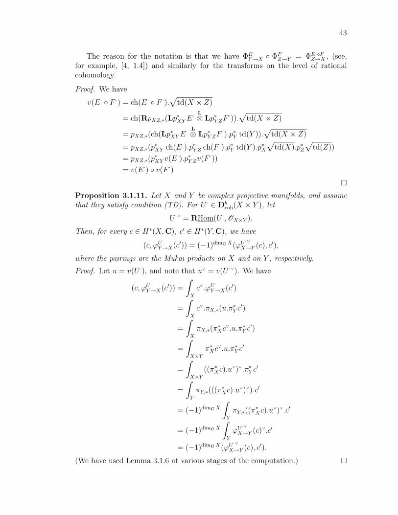
43

The reason for the notation is that we have ΦE·Y→X ΦF ·

Z→Y = ΦE·F ·Z→X , (see,

for example, [4, 1.4]) and similarly for the transforms on the level of rationalcohomology.

Proof. We have

v(E· F ·) = ch(E· F ·).√

td(X × Z)

= ch(RpXZ,∗(Lp∗XYE

· L⊗ Lp∗Y ZF

·)).√

td(X × Z)

= pXZ,∗(ch(Lp∗XYE· L⊗ Lp∗Y ZF

·).p∗Y td(Y )).√

td(X × Z)

= pXZ,∗(p∗XY ch(E·).p∗Y Z ch(F ·).p∗Y td(Y ).p∗X

√td(X).p∗Z

√td(Z))

= pXZ,∗(p∗XY v(E·).p∗Y Zv(F ·))

= v(E·) v(F ·)

Proposition 3.1.11. Let X and Y be complex projective manifolds, and assumethat they satisfy condition (TD). For U · ∈ Db

coh(X × Y ), let

U ·∨ = RHom(U ·,OX×Y ).

Then, for every c ∈ H∗(X,C), c′ ∈ H∗(Y,C), we have

(c, ϕU·

Y→X(c′)) = (−1)dimCX(ϕU·∨

X→Y (c), c′),

where the pairings are the Mukai products on X and on Y , respectively.

Proof. Let u = v(U ·), and note that u∨ = v(U ·∨). We have

(c, ϕU·

Y→X(c′)) =

∫X

c∨.ϕU·

Y→X(c′)

=

∫X

c∨.πX,∗(u.π∗Y c′)

=

∫X

πX,∗(π∗Xc∨.u.π∗Y c

′)

=

∫X×Y

π∗Xc∨.u.π∗Y c

′

=

∫X×Y

((π∗Xc).u∨)∨.π∗Y c

′

=

∫Y

πY,∗(((π∗Xc).u

∨)∨).c′

= (−1)dimCX

∫Y

πY,∗((π∗Xc).u

∨)∨.c′

= (−1)dimCX

∫Y

ϕU·∨

X→Y (c)∨.c′

= (−1)dimCX(ϕU·∨

X→Y (c), c′).

(We have used Lemma 3.1.6 at various stages of the computation.)

44

Remark 3.1.12. This result is good enough for what we need, which will be the casesof K3 surfaces and Calabi-Yau three-folds. However, it looks like there should bea better definition of the Mukai vector for arbitrary complex projective manifolds,which would take into account the canonical class of the space, and which wouldremove the requirement that the spaces satisfy (TD).

Corollary 3.1.13. Assume that X and Y satisfy (TD), and let U · ∈ Dbcoh(X ×

Y ) be such that ΦU ·Y→X is a Fourier-Mukai transform, i.e. it is an equivalence

Dbcoh(Y )→ Db

coh(X). Then ϕU·

Y→X is an isometry between H∗(Y,C) and H∗(X,C)(preserving the inner product defined in 3.1.2).

Proof. First, note that condition (TD) immediately implies that X and Y havetrivial canonical class. It is also well known that Db

coh(X) ∼= Dbcoh(Y ) implies that

X and Y have the same dimension n. Let U ·∨ = R Hom(U ·,OX×Y ), so that the

functor ΦU ·∨[n]X→Y is a left and right adjoint functor to ΦU ·

Y→X , by [5, 4.5]. But since

ΦU ·Y→X is an equivalence, Φ

U ·∨[n]X→Y must be an inverse to it, so that we must have

U · U ·∨[n] = O∆Xand U ·∨[n] U · = O∆Y

, where ∆X and ∆Y are the diagonals inX ×X and Y × Y , respectively. Therefore, using Proposition 3.1.10, we concludethat

ϕU·

Y→X ϕU ·∨[n]X→Y = ϕ

O∆XX→X ,

and

ϕU ·∨[n]X→Y ϕ

U ·

Y→X = ϕO∆YY→Y .

But it is well known (see for example [25, Chapter 6]) that ϕO∆XX→X is the identity on

H∗(X,C), and similarly for Y , so that ϕU·

Y→X and ϕU ·∨[n]X→Y are inverse to one another.

Shifting by n in the derived category has the effect of introducing a (−1)n signwhen taking the Chern character, so we conclude that ϕU

·Y→X and ϕU

·∨

X→Y are inverseto one another, up to a (−1)n sign. This fact, combined with Proposition 3.1.11shows that ϕU

·Y→X is an isometry between H∗(Y,C) and H∗(X,C).

Proposition 3.1.14. Let U · ∈ Dbcoh(X × Y ), with dimX = n, dimY = m. If

c ∈ Hp,q(Y ) then

ϕU·

Y→X(c) ∈m+n⊕k=0

Hp+k−m,q+k−m(X).

In particular, if X and Y are K3 surfaces, ϕU·

Y→X maps H2,0(Y ) to H2,0(X), and ifX and Y are Calabi-Yau threefolds, ϕU

·Y→X maps Hp,q(Y ) to Hp,q(X) for p+q = 3.

Remark 3.1.15. Throughout this entire work, our definition for a Calabi-Yau three-fold is that it is a complex, projective manifold X of dimension 3, simply connected(equivalent, through Hodge theory, to H1(X,OX) = 0), and with trivial canonicalclass (KX = 0).

45

Proof. The first statement follows immediately from the fact that

v(U ·) ∈m+n⊕k=0

Hk,k(X × Y ),

and the other two are immediate (use the fact that a Calabi-Yau has H1,0 and H0,1

zero).

We include here, for future reference, the following result due to Orlov ([36]):

Theorem 3.1.16. Let X and Y be complex projective manifolds, and let F :Db

coh(Y ) → Dbcoh(X) be an equivalence of categories. Then F is a Fourier-Mukai

transform, i.e. it is of the form ΦU ·Y→X for some object U · ∈ Db

coh(X × Y ). Fur-thermore, U · is unique up to isomorphism.

(In fact this theorem holds in the more general setting when F is full andfaithful, and has a left adjoint, but we won’t use this stronger form of the theorem.)

3.2 Equivalences of Twisted Derived Categories

In this section we give a criterion, very similar to one due to Mukai ([32]), Bondal-Orlov ([4]) and Bridgeland ([5]), for an integral functor between twisted derivedcategories to be an equivalence. We return to the situation of Definition 3.1.1, i.e.we no longer assume X and Y to be necessarily projective, nor do we assume α tobe 0. The spaces in question are still assumed to be smooth and compact.

Theorem 3.2.1. The functor F = ΦU ·Y→X is fully faithful if, and only if, for each

point y ∈ Y ,HomDb

coh(X)(FOy, FOy) = C,

and for each pair of points y1, y2 ∈ Y , and each integer i,

ExtiDbcoh(X)(FOy1 , FOy2) = 0

unless y1 = y2 and 0 ≤ i ≤ dimY . (Here Oy is the skyscraper sheaf C on y, whichis naturally an α-sheaf by 1.2.10.)

Assuming the above conditions satisfied, then F is an equivalence of categoriesif, and only if, for every point y ∈ Y ,

FOy

L⊗ ωX ∼= FOy.

Proof. The proof would be nothing more than a rewriting of Bridgeland’s excellentpaper ([5]), so we’ll not do it here. Here are some fine points about the proof (thenumbers refer to sections or theorems in [5]):

2.2. Note that since X is smooth, we have Serre duality by Theorem 2.4.3.

46

3. We don’t need to prove anything here.

4.3. If Y and S are schemes or analytic spaces, and α ∈ Br(Y ×S), then it makessense to say that an α-sheaf F is flat over S: demand that the stalks of thelocal sheaves be flat modules over the corresponding stalks of OS.

4.4. We’ll only use the statement in the same setting as in the original paper (noα-twisted version.)

4.5. Follows from the results in Sections 2.3 and 2.4.

5.1. The criterion for a complex to consist of just one sheaf supported at a pointand the fact that a composite of two Fourier-Mukai transforms is again aFourier-Mukai transform is proved like [4, 1.5] and [4, 1.4]. Note that Q isnow a complex of (p∗1α) · (p∗2α−1)-twisted sheaves on Y × Y (with p1, p2 theprojections).

5.2. Local statement on Y .

5.3. By restricting ourselves to a small enough S, we can assume that Q is nottwisted over S. Furthermore, since in the case where we apply this lemmawe actually have an open immersion i : S → Y , and for a point s ∈ S, Qs issupported at the point i(s) of Y , we see that Q can actually be taken to benon-twisted. It is important to note here that if an α-sheaf F is supportedinside an open set U such that α|U is trivial, then

Extiα-Mod(F ,F ) = ExtiMod(F ,F ),

because an α-injective resolution of F can be restricted to U to give a (non-twisted) injective resolution of F (viewed as a non-twisted sheaf now).

5.4. There is nothing special about α-sheaves here.

3.3 Moduli Spaces and Universal Sheaves

We collect in this section various results regarding the existence and constructionof absolute/relative moduli spaces, and of (possibly twisted) universal sheaves.

Theorem 3.3.1 (Existence of Relative Moduli Spaces). Let f : X → Sbe a projective morphism of C-schemes of finite type with connected fibers, and letOX(1) be a line bundle on X very ample relative to S. Then for a given polynomialP there is a projective morphism MX/S(P )→ S which universally corepresents thefunctor

MX/S : (Sch/S) → Ens,

47

which by definition associates to an S-scheme T of finite type the set of isomor-phism classes of T -flat families of semistable sheaves on the fibers of the morphismXT := T ×S X → T with Hilbert polynomial P . In particular, for any closedpoint s ∈ S one has MX/S(P )s ∼= MXs(P ). Moreover there is an open subschemeM s

X/S(P ) ⊆ MX/S(P ) that universally corepresents the subfunctor M sX/S ⊆MX/S

of families of stable sheaves.

Proof. See [25, 4.3.7].

Proposition 3.3.2. Let X/S be a flat, projective morphism, and let O(1) be arelatively ample sheaf on X/S. For a polynomial P , consider the relative modulispace M s/S of stable sheaves with Hilbert polynomial P on the fibers of X/S. Thenthere exists a covering Ui of M s (by analytic open sets in the analytic setting, andby etale open sets in the algebraic setting) such that on each X ×S Ui there existsa local universal sheaf Ui. Furthermore, there exists an α ∈ H2(M s,O∗Ms) (thatonly depends on X/S, O(1) and P ) and isomorphisms ϕij : Uj|Ui∩Uj → Ui|Ui∩Ujthat make (Ui, ϕij) into an α-sheaf (which we will call a universal α-sheaf).

Definition 3.3.3. The element α ∈ H2(M s,O∗Ms) described above is called theobstruction to the existence of a universal sheaf on X ×S M , and is denoted byObs(X/S, P ), with O(1) being understood.

Proof. For simplicity, we prove the statement in the absolute setting as the relativecase is entirely similar; also, we work in the analytic category. We use the notationsof [25, Section 4.6]. Note that Rs →M s is a principal PGL(V )-bundle ([25, 4.3.5])and hence Rs is isomorphic, locally on M s, to the product of M s and PGL(V ). If Uis any open set in M s over which Rs is trivial, say isomorphic to PGL(V )×U → U ,we can find over it GL(V )-linearized line bundles of Z-weight 1: for example,GL(V )×U → PGL(V )×U is such a line bundle. Now apply a local version of [25,4.6.2] to conclude that for every open set U of M s such that Rs ×Ms U is trivial(as a PGL(V )-bundle), there exists a local universal sheaf U on X × U .

The existence of α ∈ H2(M s,O∗Ms) and of the isomorphisms ϕij that make(Ui, ϕij) into a universal α-sheaf now follows in exactly the same way as inthe proof of [32, A.6], and the uniqueness of α is routine checking.

Proposition 3.3.4 (Mukai, [32, A.6]). Let X,M, S be proper schemes or an-alytic spaces over C, with M integral, and assume given morphisms X → S andM → S, such that X → S is projective. Let p1 and p2 be the projections to Xand M from X ×S M . For α ∈ H2(M,O∗M) assume that there exists a coherentp∗2α-twisted sheaf F on X ×SM that is flat over M . Then α is in fact in Br(M).

Proof. Using Lemma 1.2.6, represent F as (Fi, ϕij) on a cover p−12 (Ui),

where Ui is an open cover of M . Pull back a relatively ample sheaf on X/Svia p1 to get a relatively ample sheaf O(1) on X ×S M → M , flat over M . Nowusing semicontinuity, for each i we can find n0 such that for n ≥ n0 we havep2∗(Fi ⊗ O(n)) locally free on Ui. Since M is proper over C, we can choose n0

48

large enough to work for all Ui at once, so we conclude that p2∗(F ⊗ O(n)) is anα-lffr, which implies that α ∈ Br(M).

The next theorem allows us to compare the absolute and the relative settingsfor generating equivalences, when dealing with moduli problems:

Proposition 3.3.5. Let f : X → S be a morphism of schemes or analytic spaces,with S of the form SpecR for a regular local ring R. If s is the closed point ofS, let i : Xs → X be the inclusion into X of the fiber Xs over s, and let F ,G besheaves on Xs. Then

1. if ExtjXs(F ,G ) = 0 for all j then ExtjX(i∗F , i∗G ) = 0 for all j;

2. if ExtjXs(F ,G ) = 0 for all j > n0 then ExtjX(i∗F , i∗G ) = 0 for all j >n0 + dimS.

Proof. (An adaptation of the proof of [7, 3.1].) We have

R Hom·X(i∗F , i∗G ) = R Hom·Xs(Li∗i∗F ,G )

by the adjunction of Li∗ and i∗. Furthermore,

Li∗i∗F = FL⊗Xs Li∗i∗OXs

by the projection formula. Since S is smooth at s, writing down the Koszulresolution for Os and pulling back via f we get a free resolution of OXs on Xwhich can be used to compute Li∗i∗F . This gives

Hq(Li∗i∗F ) = F ⊗q∧

O⊕mXs

where m = dimS. Now the hypercohomology spectral sequence

Ep,q2 = ExtpXs(H

q(Li∗i∗F ),G ) =⇒ Hp+q(R Hom·Xs(Li∗i∗F ,G ))

= Hp+q(R Hom·X(i∗F , i∗G ))

= Extp+qX (i∗F , i∗G )

gives the results.

Part II

Applications

49

Chapter 4

Smooth Elliptic Fibrations

In this chapter we consider the first non-trivial example of an occurrence of twistedsheaves, in the construction of the twisted Poincare bundle for an elliptic fibrationwithout a section. Here we only analyze the case of fibrations without singularfibers, and investigate the relationship of our approach to Ogg-Shafarevich theory.Most of the interesting phenomena will only occur when we’ll take into accountfibrations with singular fibers, which we’ll do in Chapter 6, but this chapter shouldbe viewed as a “birational analysis” of what comes later. Also, the results in thischapter serve to illustrate some of the concepts introduced in the previous chapters.

4.1 Elliptic Fibrations

Definition 4.1.1. A smooth, projective morphism of smooth schemes (or analyticspaces), pX : X → S, such that for all s ∈ S, Xs (the fiber of pX over s) is a curveof genus one over k(s), is called a smooth elliptic fibration.

Note that although Xs has lots of points defined over k(s) when s is a closedpoint of S, Xs might not have any point defined over k(s) when s is, for example,η, the generic point of S. This will be the main issue in the study of ellipticfibrations. In fact, most of the results that will be discussed in this chapter areconcerned primarily with what happens around η, so that in many cases we’ll beable to remove the loci in S where “bad” things happen, and still get our results.

Just in order to have a specific example in mind, we give here an example of asmooth elliptic fibration.

Example 4.1.2. Let X be a general bidegree (3, 3) hypersurface in P2 ×P2, andconsider the map f : X → P2 given by projection on the first factor of the productP2×P2. Using Bertini’s theorem X is smooth and the general fiber of f is smooth.If ∆ ⊆ P2 is the discriminant locus of this fibration (the locus over which the fiberis not smooth), and if S = X \∆, then XS = X ×P2 S → S is a smooth ellipticfibration.

In this example we can in fact see that f does not have a rational section.Indeed, the closure of a rational section over all of P2 would be a divisor D in

50

51

X which would intersect a general fiber of the map X → P2 in one point. ButLefschetz’s theorem tells us that the map Pic(P2 × P2) → Pic(X) is surjective.Since all divisors in Pic(P2 ×P2) have intersection number with the general fiberof X → P2 divisible by 3, we conclude that we cannot find a rational section inXS → S. On the other hand, the pull-back of the general hyperplane section ofthe second factor of P2 × P2 provides an example of a 3-section (a flat, effectivedivisor that meets each fiber in 3 points).

Therefore we conclude that Xη has no rational points (a rational point wouldcorrespond to a rational section of XS → S), but that it has a rational divisor ofdegree 3 (corresponding to the 3-section).

4.2 The Relative Jacobian

Given a smooth elliptic fibration pX : X → S, there is a naturally constructedelliptic fibration pJ : J → S that has the same fibers as X → S over the closedpoints of S, but which has a section. This fibration, called the relative Jacobian ofX → S is in a certain sense a universal object, and it will constitute the startingpoint of our study of smooth elliptic fibrations.

Definition 4.2.1. Fix a relatively ample sheaf OX(1) for the morphism pX : X →S, and let pJ : J → S be the relative moduli space of semistable sheaves of rank1, degree 0 on the fibers of pX (see Theorem 3.3.1 for existence and properties).The fibration J → S (which is a smooth elliptic fibration) is called the relativeJacobian of X → S.

Proposition 4.2.2. The map pJ is a smooth elliptic fibration with a section. Overa closed point s ∈ S, we have Js ∼= Xs. If we set L = pJ,∗ωJ/S, then any smoothelliptic fibration p′ : J ′ → S possessing a section, having J ′s

∼= Xs for all closedpoints s ∈ S, and for which p′∗ωJ ′/S

∼= L , is isomorphic (over S) to J → S.

Proof. The map pJ is a flat, projective morphism by the very definition of relativemoduli spaces. The flat family OX of sheaves of rank 1, degree 0 on the fibers ofpX gives by the universal property of J → S a map s0 : S → J which is a sectionof pJ . The fiber Js of pJ over a closed point s ∈ S is isomorphic to Pic(Xs), andsince Xs is a smooth elliptic curve over an algebraically closed field, we concludethat Js ∼= Xs. The smoothness of J follows at once from local dimension estimates(see [25, Section 4.5]). Therefore pJ is a smooth elliptic fibration.

Now we can apply [13, 2.2 and 2.3] to J ′ → S to obtain the uniqueness propertyof pJ . Note that since all the fibers of pX are connected, the same holds for pJ ,and therefore the birational morphism g that is given to us by [loc.cit.] is in factan isomorphism.

A final note: since locally (in the etale or analytic topologies) pX has sec-tions (because there are no multiple fibers), this proof actually shows that X islocally isomorphic to J , over S. We’ll give a direct proof of this fact in the nextproposition.

52

Proposition 4.2.3. Assume that pX has a section s : S → X. Then J and X areisomorphic as schemes or analytic spaces over S; an isomorphism ϕ : X → J canbe chosen in such a way that the natural section s0 of pJ (that corresponds to OX

on X) is mapped to s. The moduli problem is fine, under these circumstances, anda universal sheaf can be taken to be

OX×SJ(Γ)⊗ π∗XOX(−s),

where Γ is the (scheme theoretic) graph of ϕ inside X ×S J , πX : X ×S J → X isthe projection, and OX(−s) is the line bundle on X defined by the divisor −s, theimage of the section s : S → X.

Proof. This is nothing more than a relative version of the corresponding, wellknown statement for elliptic curves. This definition only works here for smoothelliptic fibrations (because Γ is a Cartier divisor). In the general case we’ll haveto replace OX×SJ(Γ) with I ∨

Γ , the dual of the ideal sheaf of Γ (which makes sensealways).

This identification allows us to give an explicit construction of the Jacobian ofX → S. For simplicity we’ll work in the analytic category. Cover S with opensets Ui such that if we set Xi = X ×S Ui, the projection Xi → Ui admits a section.For each i, fix once and for all a section si : Ui → Xi. We identify si with itsimage in Xi, whenever there is no danger of confusion. It is a divisor in Xi, whoserestriction to each fiber has degree 1.

We digress to talk about translations on elliptic curves. Let C be a smoothcurve of genus 1 over an algebraically closed field (i.e., an elliptic curve, but withoutthe choice of an origin). On C there exists a natural identification between linebundles of degree 0 and translations of C (under the group law on C that isobtained by fixing some origin), which is independent of the choice of an origin.This identification can be described as follows: let L ∈ Pic(C); fixing an origins0 ∈ C, L can be written in a unique way as L ∼= OC(s0 − p) for some p ∈ C.The translation associated to L , τL , is x 7→ x+ p for x ∈ C, where the operationis the one given in the group law of C, with origin fixed at s0. It is a trivial checkto see that τL is in fact independent of the choice of s0.

Conversely, given a translation τ , we can associate to it an element Lτ ofPic(C) by the formula

Lτ = τ ∗(F )⊗F−1,

where F is some line bundle of degree 1 on C. This is independent of the choiceof F , and the operations L 7→ τL , τ 7→ Lτ are inverse to one another. The im-portant property of Lτ is the following: if F is a line bundle on C (not necessarilyof degree 0), then we have

τ ∗F ∼= F ⊗L deg Fτ .

A consequence of this formula is that if F ∈ Pic(C), then τ ∗F ∼= F , so if C ′ isisomorphic to C via a translation, there is a well defined notion of pull-back of F

53

to C ′, independent of the choice of translation: all pull-backs will give the sameline bundle (up to isomorphism).

We now return to the initial situation. Define Uij = Ui ∩ Uj, Xij = Xi ∩ Xj,and similarly Uijk, Xijk, etc. On each Xij there are two sections, si and sj, whichdefine the line bundle

Lij = OXij(sj − si),

whose degree along the fibers of Xij → Uij is zero. As such it defines a translationτij : Xij → Xij over Uij. It is useful to note that τji = τ−1

ij , and τij τjk τki = idon Xijk.

We think of these translations as gluing functions for a new space J , obtainedfrom the “slices” Xi, glued along

τij : Xj|Xi∩Xj → Xi|Xi∩Xj .

Since the compatibility relations (checked above) hold, we can actually glue to-gether this space, and it obviously comes with a natural map pJ : J → S whichmakes it into a smooth elliptic fibration. This construction naturally provides uswith isomorphisms ρi : Ji → Xi over Ui, that satisfy

ρi ρ−1j = τij

over Xij. The images of the sections si ⊆ Xi and sj ⊆ Xj, under ρ−1i and ρ−1

j ,coincide in Jij: indeed, this is because we have

ρi ρ−1j (sj) = τij(sj) = sj − (sj − si) = si.

(We have written here −(sj − si) for τij = τO(sj−si), to make things more evident.)Therefore the images of all the local sections under the local isomorphisms gluetogether in J to give a global section t0 of J .

Now we can see how a point p ∈ J that lies over a point s ∈ S corresponds toa line bundle on Xs: let Ui be an open set such that s ∈ Ui, and associate to pthe line bundle ρ∗iOJs(p− t0(s)). Since this line bundle has degree 0, the resultingline bundle on Xs does not change if we make another choice for the open set inwhich s lies, say Uj. In that case, we would obtain ρ∗jOJs(p − t0(s)), and the twoline bundles differ by the pull-back by a translation of Xs. Since we are workingwith line bundles of degree 0, the isomorphism type of the result is not affected bythis operation.

4.3 The Twisted Poincare Bundle

We consider the question of the existence of a universal sheaf on the productX ×S J , since in this setting we can explicitly construct (as a gerbe) the twistingα of Definition 3.3.3.

54

We continue with the notations and assumptions from the previous section. LetPi = Xi ×S Ji, and similarly Pij, etc. Note that over each Pi we have a universalsheaf given by

Ui = OX×SJ(Γi)⊗ π∗XOXi(−si),

as in Proposition 4.2.3. (We abuse the notation and keep using πX for the projec-tion Xi → Ui.)

The natural question to ask at this point is why don’t these local universalsheaves glue to a global one? We need to look over an intersection Pij, and seewhat is the failure of Ui|Pij and Uj|Pij to be isomorphic.

LetMij = Uj|Pij ⊗U −1

i |Pij ,

an operation which we can do in this case since we are dealing with line bundles;we have

Mij = π∗XOXi(si − sj)⊗ O(Γj)⊗ O(Γi)−1.

Let p be any point in Jij, let s be its image in S, and consider the restriction ofMij to Xs. It is isomorphic to

OXs(si − sj + ρj(p)− ρi(p)),

which is trivial along Xs (we could have seen this also from the fact that Ui andUj are local universal sheaves, so over p ∈ Jij they must give the same line bundleon Xs, the one represented by p as a point of the moduli space J).

We conclude that Mij is the pull-back of a line bundle Fij from Jij. Thecollection Fij, viewed as a gerbe α ∈ H2(J,O∗J) will represent the twisting thatis the obstruction to the existence of a universal sheaf on X ×S J .

It is worthwhile to note that the twisting π∗Jα is in fact trivial on X ×S J :indeed, the collection Uij is a π∗Jα-twisted line bundle on X ×S J , so α musthave order divisible by 1 (the rank of this vector bundle). In other words α mustbe trivial. The point here is that although we could modify this line bundle tomake it glue well on X ×S J , this operation would not preserve the fibers of thisbundle on fibers of πJ , so the result would no longer be a universal sheaf.

It is not hard to see that the isomorphism type of Fij (at least along the fibersof Jij → S) can be described as follows: if on Xij we consider the sheaf

L −1ij = OXij(si − sj),

then Fij is isomorphic to the sheaf ρ∗iL−1ij . The remarks in the previous section

regarding the invariance of line bundles of degree zero under translations show thatthis gives a well-defined isomorphism type for Fij. An easy verification shows thatthe collection ρ∗iL −1

ij satisfies the conditions to form a gerbe.However, this construction is not entirely natural: we have made the choice of

using ρi as an isomorphism between Jij and Xij. In fact, the verification that wecan do to ensure that Fij is indeed a gerbe only tests this along the fibers of

55

Jij → S. This means that if Fij were twisted by line bundles from Uij, we wouldnot be able to detect this. To make this construction independent of choices, onecould consider the sheaves

Fij = πJ,∗Mij.

These only differ from the Fij’s constructed before by the global line bundle

πJ,∗OX×SJ ,

and therefore the gerbe determined by Fij is the one we want. Under thisdefinition of Fij it is obvious that the compatibility relations are satisfied.

This situation should be contrasted to the one in the next section, where Ogg-Shafarevich theory produces a natural element of Br(J)/Br(S). This should bethought of as meaning that by just looking at the picture along the fibers (whichis what we did in this section) we can only recover α up to possible twists fromBr(S).

4.4 Ogg-Shafarevich Theory

As alluded to at the end of the previous section, this picture has a strong rela-tionship to the classification theory for elliptic fibrations, as developed by Ogg andShafarevich. For a reference to the technical aspects of this theory, see [13].

The setup is as before: X → S is a smooth elliptic fibration, and J → S is itsrelative Jacobian fibration. Since X → S is obtained from J → S by the “cut andreglue” procedure described before, one can try to understand this process froma cohomological point of view. One approach is to note that the regluing dataconsists of translations along the fibers of each Ji; the group of these translationscan be identified with the group J#(Ui) of sections of Ji → Ui (which can benaturally given the structure of a group because we have a fixed, natural sectiont0 of J → S). Therefore the data needed to reconstruct the fibration X → S outof J → S is an element αX of the Tate-Shafarevich group of J , XS(J), defined as

XS(J) = H1(S, J#),

where J# is the sheaf of abelian groups on S defined by

J#(U) = the group of sections of JU → U.

This makes sense in any topology, and if one considers everything in the analyticor etale topology, one obtains a 1-1 correspondence between elliptic fibrationsX → S whose Jacobian is J → S, and elements of XS(J). (It is importantto note here that some fibrations that correspond to elements of H1

an(S, J#) canonly be constructed in the analytic category and have no algebraic counterpart; toremain inside the algebraic category one has to work with in the etale setup, andthus obtain fewer elliptic fibrations.)

56

The next step is to understand this picture further, and using the Leray spectralsequence one shows that if the fibrations in question have no singular fibers thereis an exact sequence

0→ Br(S) −→ Br(J)π−→XS(J)→ 0

which splits. (The first map is just the pull-back map on the Brauer groups.) Thesplitting is provided by, say, the pull-back from J to S via a section of J → S.

Let’s see how this relates to the situation described in the previous section:the construction of the gerbe α provides an element of Br(J), and projecting weobtain an element π(α) of XS(J). In fact, the line bundles ρ∗iOXij(si − sj) canbe written in a unique way as OJij(tij − t0) for some tij ∈ J#(Uij), and it is clearfrom the construction that in order to reconstruct X → S one needs to reglue theJi’s via the translations

τ−1ij = τOJij (tij−t0)

which are the inverses of the translations τij used before to construct J from X.But the translations τ−1

ij give the element αX of XS(J) that represents X(see the construction described above), and tracing through all the identificationsit is easy (!) to see that αX is precisely the projection π(α) of α.

Therefore we obtain:

Theorem 4.4.1. Let X → S be a smooth elliptic fibration, and let J → S be itsrelative Jacobian. Let αX ∈XS(J) be the element of the Tate-Shafarevich groupthat represents X → S, and let α ∈ Br(J) be the obstruction to the existence ofa universal sheaf on X ×S J (for the moduli problem on X that gives J). ThenαX = π(α), where π is the projection

0→ Br(S) −→ Br(J)π−→XS(J)→ 0.

Theorem 4.4.2. Let n denote the smallest positive fiber degree of a divisor on X.(The fiber degree of a divisor D is defined as the degree of the restriction D|F ofD to a fiber of X → S.) Then the projection αX = π(α) is n-torsion in XS(J).

Proof. Since we work in the Tate-Shafarevich group we can ignore contributionsfrom the Brauer group of the base, and we only need to prove that there exist linebundles Li on Ji such that

F⊗nij∼= Li ⊗L −1

j

on Jij. (This proves that, up to contributions from Br(S), the gerbe Fij definedin the previous section is trivial.)

Let D be a divisor on X of fiber degree n, and let L = OX(D). Define

57

Li = ρ∗iL−1|Xi . Then we have

Li ⊗L −1j = ρ∗iL

−1 ⊗ ρ∗jL= ρ∗i (L

−1 ⊗ (ρ−1i )∗ρ∗jL )

= ρ∗i (L−1 ⊗ τ ∗jiL )

= ρ∗i (L−1 ⊗L ⊗L ⊗n

τji)

= ρ∗i (L−1 ⊗L ⊗L ⊗n

ji )

= ρ∗iOX(si − sj)⊗n

= F⊗nij ,

where we have used the comments in Section 4.2 regarding translations of linebundles of various degrees. (Note that we have used the fact that deg L = n.)

Remark 4.4.3. In fact, using some slightly more detailed information that one canget from Ogg-Shafarevich theory it can be proven that the order of αX in XS(J)is precisely n.

4.5 Other Fibrations

The Jacobian fibration that we considered in the previous sections is not the onlyone we can naturally construct from the original fibration X → S. In a certainsense the Jacobian is the common denominator of the other ones, but these presentsome interest as well, and we study them briefly here.

We keep the notation from the previous sections.

Definition 4.5.1. For any integer k, let Y → S be the relative moduli space ofsemistable sheaves of rank 1, degree k on the fibers of X → S. We call Y → S thek-th twisted power of X → S, and denote it by Xk → S.

Theorem 4.5.2. For any integer k, Xk → S is a smooth elliptic fibration whoserelative Jacobian is isomorphic in a natural way to the relative Jacobian J → S ofthe initial fibration X → S. If α ∈XS(J) is the element of the Tate-Shafarevichgroup representing X → S, then Xk → S is represented by αk. Consequently thefibration (Xk)k

′ → S is isomorphic to Xkk′ → S. Let n denote the order of α inXS(J). A universal sheaf exists on X ×S Xk if and only if

(k, n) = 1,

and in this case X can be viewed as a moduli space on Xk (we have

X ∼= (Xk)k′

as fibrations over S, where k′ is any integer such that kk′ = 1 mod n).

58

Proof. Note that Xk → S is naturally an elliptic fibration, because the modulispace of rank 1, degree k semistable sheaves on an elliptic curve is isomorphicto the curve itself. This also proves that over each closed point s ∈ S we haveXks∼= Xs. In fact, the same construction as in Proposition 4.2.3 shows that Xk

and X are locally isomorphic over S. (The universal sheaf in this case is given by

U = OX×SXk(Γ)⊗ π∗XOX((k − 1)s),

where s is the local section.)Recall that we have a cover of S by open sets Ui, such that the restrictions

Xi → Ui have sections si : Ui → Xi. In order to construct J we reglued thesepieces via translations

τij : Xj|Xi∩Xj → Xi|Xi∩Xj ,

which were associated to the line bundles on Xi ∩Xj

Lij = OX(sj − si).

In order to construct Xk we replace these translations by

τij : Xj|Xi∩Xj → Xi|Xi∩Xj ,

associated to the line bundles

Lij = OX((k − 1)(si − sj)).

It is not hard to see that the τij’s again satisfy the compatibility relations, so wecan use them to reglue the slices Xi to a global space Y which has a natural mapY → S, and consists of local slices Yi over Ui. These slices are isomorphic to theinitial slices Xi via isomorphisms (of spaces over S)

ρi : Yi → Xi,

which satisfyρi ρ−1

j = τij.

We claim that Y is globally isomorphic to Xk. The universal sheaves that weconstructed before give isomorphisms

ϕi : Yi → Xki

(where Xki = Xk ×S Ui) by the universal property of Xk, and all we need to prove

is that the ϕi’s glue together to a global isomorphism ϕ : Y → Xk.Let ti = ρ−1

i si : Ui → Yi, the section of Yi that corresponds to the originalsection si on Xi. Since the gluings are only translations, in order to show that ϕiand ϕj agree on Yij it suffices to show that ϕi(ti) = ϕj(ti) on Yij.

59

It is easy to see that ϕi(ti) = [OXi(ksi)]. (We have abused the notation seriouslyhere: OXi(ksi) is a line bundle of degree k on the fibers of Xi → Ui, and as suchit gives a map Ui → Xk

i . The image of this map is [OXi(ksi)].) Also, we have

ϕj(ti) = [OXi∩Xj(ρj(ti) + (k − 1)sj)].

Therefore we need to prove that

OXi∩Xj(ρj(ti) + (k − 1)sj) ∼= OXi∩Xj(ksi).

Note that we haveτijρj(ti) = ρi(ti) = si

and thusρj(ti) = τji(si).

Hence we have

O(ρj(ti) + (k − 1)sj) = O(τji(si) + (k − 1)sj)

= τ ∗ijO(si)⊗ O((k − 1)sj)

= O(si + (k − 1)(si − sj) + (k − 1)sj)

= O(ksi),

which is what we needed.Now we can prove the rest of the claims: since Xk

s∼= Xs for all closed points

s ∈ S, in order to prove that Xk and X have isomorphic Jacobians we only needto show that pXk,∗ωXk/S

∼= pX,∗ωX/S (use Proposition 4.2.2). But this follows atonce from the fact that along any elliptic curve C, the action of a translation τis trivial on a global section of ωC . Since Xk is obtained by regluing slices of Xalong translations, this shows that pXk,∗ωXk/S and pX,∗ωX/S are glued together inthe same way along the intersections Uij.

Now let µi : JX,i → Xi be the isomorphisms that take the canonical sectionof the Jacobian of X, JX to the local sections si in Xi. (These isomorphismswere called ρi in Section 4.2.) Also, let µki : JXk,i → Xk

i be the correspondingmorphisms that take the section of JXk to ti. Composing, we get an isomorphismϕ : JX → JXk given by

ϕ = (µki )−1 ρ−1

i µi(it is not hard to see that these isomorphisms glue together.) We’ll compareBr(JXk) and Br(JX) using this isomorphism.

The twisting in J associated to Xk is given by

(µki )∗OXkij

(ti − tj),

60

Applying (ρ−1i )∗ we get

(ρ−1i )∗OXk

ij(ti − tj) = OXij(ρi(ti)− ρi(tj))

= OXij(si − τij(sj))= OXij(si)⊗ OXij(τij(sj))

−1

= OXij(si)⊗ τ ∗jiOXij(−sj)= OXij(si)⊗ OXij(−sj)⊗L −1

ji

= OXij(si)⊗ OXij(−sj)⊗ OXij((k − 1)(si − sj))= OXij(k(si − sj)),

and thus

ϕ∗(µki )∗OXk

ij(ti − tj) = µ∗i (ρ

−1i )∗OXk

ij(ti − tj)

= µ∗iOXij(k(si − sj)),

which shows that if X is represented by α ∈XS(JX), then Xk is represented by(ϕ−1)∗αk in XS(JXk).

The result about the existence of a universal sheaf is known (see, for exam-ple, [6]). But here is a quick proof of the existence of a universal sheaf when(k, n) = 1: we only need to show that we can twist the universal sheaves describedin the beginning of the proof in a way that would make them glue. A computationsimilar to the one done in Section 4.3 shows that

Mij = Uj|Pij ⊗U −1i |Pij

is equal to the pull-back of a line bundle Fij from Xkij, and Fij can be taken to

be of the formρ∗iL

−1ij = ρ∗iOXij((k − 1)(sj − si)).

Now let S be a line bundle on X, of fiber degree n (such a line bundle existsglobally on X, by the comments at the end of the previous section), and considerthe line bundles S ′

i = ρ∗iSi (where Si = S |Xi). We have

(ρ−1j )∗(S ′

j ⊗ (S ′i )−1) = Sj ⊗ τ ∗ijS −1

i

= Sj ⊗S −1i ⊗L ⊗−n

ij

= OXij(−n(k − 1)(si − sj)).

Therefore, considering the collections of line bundles OXki(ti) and S ′

i , wesee that their coboundaries are O(k(si−sj)) and O(−n(k−1)(si−sj)) (wherewe have omitted the subscript Xij and the pull-backs by isomorphisms to Xk

because these do not matter, since we are dealing with line bundles of degree 0).Since k and −n(k−1) are coprime, we can obtain any multiple of O(si−sj) outof them, in particular we can construct O((k − 1)(sj − si)), which we have seenis the obstruction to gluing the Ui’s together. Therefore this obstruction is trivial,and hence the Ui’s can be glued to form a global universal sheaf, thus finishingthe proof.

61

Remark 4.5.3. Note that we have fixed a special isomorphism of JX and JXk inorder to obtain this result. This is what allows us to distinguish between X andX−1, which are isomorphic, even as fibrations over S! Indeed, one can take I∆

as a universal sheaf on X ×S X, where ∆ is the diagonal in X ×S X. But in thiscase, the isomorphism between JX and JX−1 is doing a negation along the fibers,which also acts by −1 on the Brauer group. Note that this answers the questionposed at the end of [13, Section 1].

Another consequence of this remark is that if the j invariant is not constant(so that the only automorphisms of J/S are given by translations and negation),and k is not equal to 1 or −1 in Z/nZ, then Xk is not isomorphic to X, even atthe generic point of S. Thus if we can prove that there is only one elliptic fibrationstructure whose Jacobian is the same as that of X among all birational modelsof X, then X is not birational to Xk. (Because, if they were birational to eachother, they would have to be isomorphic to one another because they have thesame Jacobian, and this is impossible.) See also Section 6.7.

Chapter 5

K3 surfaces

In this chapter we apply the general results deduced in Part I to different situ-ations related to K3 surfaces. The reason K3 surfaces provide an interesting setof examples is because, on one hand, we have a good explicit description of theirmoduli space (the Torelli theorem, 5.1.1) so we can handle them easily in terms oflattices and Hodge structures, and, on the other hand, moduli spaces of sheaves onK3’s are well understood, primarily through the work of Mukai ([32]) (see the in-troductory section 5.1). Furthermore, it is also known when two K3 surfaces haveequivalent derived categories (of untwisted sheaves), by the work of Orlov ([36]).

The first section presents the known results about K3 surfaces, moduli spacesof sheaves on them, and derived categories of untwisted sheaves. Everything elseis built upon these facts. We have seen in Chapter 4 that one can recover theclassical Ogg-Shafarevich theory of elliptic fibrations without a section by studyingthe obstruction to the existence of universal sheaves for certain moduli problems.For K3 surfaces, we can do better: in most cases we don’t need an elliptic fibrationon the K3 to play the same game. In Section 2 we study deformations of vectorbundles as twisted sheaves, obtaining results that will be used in identifying theobstruction. These results are also interesting on their own, in the context ofdeformation theory of vector bundles.

Section 3 contains the main technical result of this chapter, an explicit descrip-tion of the obstruction α (whose existence is asserted in Theorem 3.3.2) to theexistence of a universal sheaf for an arbitrary moduli problem on a K3 X, whenthe moduli space is again a K3. This description is given in purely cohomologicalterms, via Fourier-Mukai transforms.

By analogy with Ogg-Shafarevich theory, one can also attempt to reverse theprocess of going from the pair (X, v) (where X is a K3, and v is the data for a mod-uli problem on X) to the pair (M,α) (where M = M(v) is the moduli space, andα is the obstruction to the existence of a universal sheaf on X ×M). This is whatwould be needed in order to obtain a complete generalization of Ogg-Shafarevichtheory in terms only of moduli problems and obstructions. Unfortunately, we can-not push this too far. The best we can do is to find the transcendental lattice ofthe candidate X, together with its Hodge structure. In most cases, this should

62

63

allow us to get X; however, finding v seems a more difficult problem.The last section deals with the relationship of the results of the previous sections

with the topic of equivalences of derived categories. This provides an insight intowhy we can only get a hold of the transcendental lattice of X in generalizing Ogg-Shafarevich theory. As a consequence of this analysis we also observe the followingcurious phenomenon: when we can find X and v, X only depends on the cyclicsubgroup of Br(M) generated by α. This allows us to infer that in some cases onehas

Dbcoh(M,α) = Db

coh(M,αk)

for (k, ord(α)) = 1, a rather striking application of the theoretical results of theprevious chapters. In the next chapter we’ll see a similar result for elliptic Calabi-Yau threefolds.

5.1 General Facts

The main results about K3 surfaces: the Torelli theorem, Mukai’s calculation ofmoduli spaces of sheaves on K3’s, Orlov’s characterization of derived equivalencesfor K3’s – are all presented in this section, and put in the context of the results inthe first part.

The Torelli Theorem

Let’s fix notation: let X be a complex K3 surface, i.e., a complex manifold ofcomplex dimension 2, having trivial canonical class (KX = 0) and being simplyconnected (equivalent, using Hodge theory, to having H1(X,OX) = 0).

We have H2(X,Z) = Z22, and considering this group with the intersectionpairing we obtain a lattice which is isomorphic to

LK3 = (E8)⊕2 ⊕ (U(1))⊕3.

Inside the H2(X,Z) lattice there are two natural sublattices, the Neron-Severisublattice of X, NS(X), (consisting of first Chern classes of holomorphic vec-tor bundles), and its orthogonal complement, the transcendental lattice TX =NS(X)⊥. Both these lattices are primitive sublattices of H2(X,Z), but may benon-unimodular.

The complex structure of X is reflected in its Hodge decomposition

H2(X,C) = H2,0(X)⊕H1,1(X)⊕H0,2(X).

We have dimH2,0(X) = 1, so in order to specify this decomposition, it is enoughto specify a one-dimensional complex subspace π ⊆ H2(X,C) (called the period ofX): indeed, one can take H2,0(X) to be π, H0,2 to be the complex conjugate π ofπ, and H1,1 to be the orthogonal (with respect to the intersection pairing) to thespan of π and π. The complex subspace π satisfies the following extra property: ifv ∈ π is a non-zero vector, we have v.v = 0 and v.v > 0.

64

Two lattices L,L′, endowed with Hodge structures, are said to be Hodge iso-metric if and only if there is an isometry between the two preserving the Hodgestructures on them.

Theorem 5.1.1 (Torelli for K3’s). Two K3 surfaces, X and Y , are isomorphicif and only if the lattices H2(X,Z) and H2(Y,Z) are Hodge isometric. For allperiods π in LK3 ⊗C satisfying π.π = 0 and π.π > 0, there exists a K3 surface Xwhose period is π, under some choice of isomorphism between H2(X,Z) and LK3.

There is yet another part to this theorem, which explains the relationship be-tween the group of Hodge isometries H2(X,Z) → H2(X,Z) on a K3 X, and thegroup Aut(X) of automorphisms of X: the former group is generated by Aut(X),and by a certain class of automorphisms of H2(X,Z), called (−2)-reflections. Formore details about the Torelli theorem for K3 surfaces, the reader should con-sult [3].

This shows how we can construct a moduli space for K3 surfaces: we takethe subspace of vectors v in LK3 ⊗ C satisfying v.v = 0, v.v > 0, and then weprojectivize it; it is a quasi-projective variety. Call it P . The automorphism groupof the lattice LK3 acts on P ; let M = P/Aut(LK3). Then M is a coarse modulispace for K3 surfaces.

Note that many (most) complex K3 surfaces are not algebraic: in order to bealgebraic they would have to be projective, i.e. have at least an ample divisor,and therefore at least a non-zero divisor. But most K3’s don’t have any non-zerodivisors at all: these would correspond to classes in H1,1(X) ∩H2(X,Z), and theset of periods for which this group is non-trivial is a countable union of codimensionone subspaces of M .

Since we are mainly interested in algebraic K3’s, we only make precise thesestatements in the context of primitively polarized K3 surfaces, described below.These results are taken from [25] and [32].

Definition 5.1.2. Let d be a positive integer. Let Kd be the functor (Sch/C) →Ens that maps a scheme Y to the set of equivalence classes of pairs (f : X → Y,L )such that f : X → Y is a smooth family of K3 surfaces, L is a line bundle onX, and for any t ∈ Y , the restriction Lt of Lt to the fiber Xt = f−1(t) is anample primitive line bundle with c2

1(Lt) = 2d. Two pairs (f : X → Y,L ) and(f ′ : X ′ → Y,L ′) are equivalent if and only if there exists a Y -isomorphismg : X → X ′ and a line bundle N on Y such that g∗L ′ ∼= L ⊗ f ∗N .

Theorem 5.1.3. The functor Kd is corepresented by a coarse moduli space Kdwhich is a quasi-projective, irreducible scheme.

Moduli Problems and Mukai’s Results

Definition 5.1.4. Let X be a K3 surface. The Mukai lattice of X is defined to be

H(X,Z) = H0(X,Z)⊕H2(X,Z)⊕H4(X,Z),

65

endowed with the product

((r, l, s), (r′, l′, s′)) =

∫X

r.s′ + r′.s− l.l′,

where the dot product on the right hand side is the cup product in H∗(X,Z).The Hodge decomposition on H(X,Z) is given by

H2,0(X) = H2,0(X)

H1,1(X) = H0(X,C)⊕H1,1(X)⊕H4(X,C)

H0,2(X) = H0,2(X)

Elements in H1,1(X) will be called algebraic.We’ll sometimes also consider H(X,Q) = H(X,Z)⊗Q, with intersection pro-

duct and Hodge decomposition defined in a similar fashion.For a coherent sheaf E (or, more generally, an element of Db

coh(X)), definev(E ) ∈ H(X,Z) by

v(E ) = ch(E ).√

td(X) = (rk(E ), c1(E ), rk(E )ω +1

2c1(E )2 − c2(E )),

(where ω ∈ H4(X,Z) is the fundamental class of X). This element is called theMukai vector of E .

Remark 5.1.5. Note that the intersection product and the Mukai vector are thesame as the more general ones introduced in Section 3.1, restricted to the latticeH(X,Z). Therefore all the results obtained there apply.

The reason one studies these objects is because one is interested in studyingmoduli spaces of semistable sheaves on X. The following results are mainly dueto Mukai ([32]). (Some have been rephrased in the more convenient language ofsheaves of modules over an Azumaya algebra.)

Theorem 5.1.6. Let X be a K3 surface, with a fixed polarization P. Let v ∈H(X,Z) be a primitive (indivisible) vector that lies in the algebraic part of H(X).Assume that v is isotropic (i.e. (v, v) = 0), and that the moduli space of semistablesheaves of Mukai vector v, M(v), is non-empty and does not contain any properlysemistable points. Then M(v) is a K3 surface.

Example 5.1.7. Just for the purpose of having an example in mind, we includehere the following construction due to Mukai ([34, 2.2]). Consider a net of quad-rics in P5, generated by three non-singular quadrics Q1, Q2, Q3, and assume thatthese intersect transversely. Taking the net general enough the intersection of thequadrics in this net is a smooth K3 surface.

Each smooth quadric Q in the net is isomorphic to G(2, 4), the Grassmanianof planes in C4 and as such it has two vector bundles of rank 2 on it, TQ and QQ

(the tautological and the quotient bundles). Consider their restrictions TQ|X and

66

QQ|X . After a fixed twist of one of them by a line bundle, it can be arranged thatthey have the same Chern classes, call them c0, c1, c2.

Mukai proves that these vector bundles are stable, and that they are all differentfor different quadrics (and among themselves). However, when the quadric becomessingular, the two bundles become isomorphic with each other. These are all thesemistable sheaves with Chern classes c0, c1, c2.

The geometric picture one gets from this is that the moduli space of semistablesheaves with these Chern classes consists of a double cover of the space of quadrics,branched over the discriminant locus. The space of quadrics in question is P2 (weare talking about a net!), and the discriminant locus is a sextic curve in this P2.Therefore the moduli space is isomorphic to a double cover of P2 branched over asextic, which is again a K3 surface.

Definition 5.1.8. Under the assumptions of the previous theorem, let M = M(v),and let α ∈ Br(M) be the obstruction of Definition 3.3.3 for this moduli problem.We’ll denote α by Obs(X, v). Theorem 3.3.2 shows the existence of a π∗Mα-twisteduniversal sheaf U on X ×M (where πM : X ×M →M is the projection). Let Abe an Azumaya algebra on M representing α, and using the equivalence betweentwisted sheaves and modules over an Azumaya algebra, represent U as a sheaf Uof modules over π∗MA .

Then U is called a quasi-universal sheaf. It has the property that

U |X×[F ]∼= F⊕n

for some n that only depends on U (the isomorphism is as sheaves of OX-modules).This n is called the similitude of U , denoted by s(U ). (Here, F is a semistablesheaf on X with Mukai vector v, and [F ] is the point of M that corresponds toit.)

In fact, U satisfies a certain universal property which is very similar to thatenjoyed by a universal sheaf; see [32, Appendix 2].

Definition 5.1.9. The cohomological Fourier-Mukai transform associated to Uis the homomorphism

ϕ = ϕU ∨

X→M : H(X,Q)→ H(M,Q)

given by

ϕ( · ) =1

s(U )πM,∗(π

∗X( · ).v(U ∨)),

where

U ∨ = RHom(U ,OX×M),

and

v(U ∨) = ch(U ∨).√

td(X ×M).

67

Theorem 5.1.10. Under the hypotheses of Theorem 5.1.6, the map ϕ is a Hodgeisometry between H(X,Q) and H(M,Q). It maps v ∈ H(X,Q) to the vector(0, 0, ω) ∈ H(M,Q), and it therefore induces a Hodge isometry

v⊥/v ∼= H2(M,Q),

the latter being computed inside H(X,Q). Restricted to v⊥/v, this isometry isindependent of the choice of quasi-universal bundle and is integral, i.e. it takesintegral vectors to integral vectors. It therefore induces a Hodge isometry

H2(M,Z) ∼= v⊥/v,

the latter now computed in H(X,Z).

Remark 5.1.11. Using the Torelli theorem, this gives a complete description of themoduli space M .

Proof. When the moduli problem is fine, one first proves that U (the universalsheaf) induces an equivalence of derived categories Db

coh(X) ∼= Dbcoh(M). We’ll

do this in a more general context, in Theorem 5.5.1. Then the result followsimmediately from the results in Section 3.1. The general case (when the moduliproblem is not fine) is done by a deformation argument in [25, Chapter 6].

Theorem 5.1.12. Let n be the greatest common divisor of the numbers (u, v),where u runs over all H1,1(X) ∩ H(X,Z). Then the following statements hold:

1. There exist α-twisted locally free sheaves on M of ranks r1, r2, . . . , rk, withgcd(r1, r2, . . . , rk) = n, and therefore α is n-torsion. (α is the obstructiondescribed in Definition 5.1.8.)

2. Denote by ϕ any cohomological Fourier-Mukai transform defined above (forsome choice of quasi-universal sheaf). Then ϕ maps TX into TM , (viewingTX as a sublattice of H(X,Z) via the inclusion λ 7→ (0, λ, 0)), and ϕ|TX isindependent of the choice of quasi-universal bundle used to define it.

3. There exists λ ∈ TX such that v + λ is divisible by n (in H(X,Z)); for sucha λ we have ϕ(λ) divisible by n (in TM).

4. ϕ is injective, and its cokernel is a finite, cyclic group of order n, generatedby ϕ(λ)/n for any λ satisfying the condition in (3).

Example 5.1.13. In Example 5.1.7 the number n = 2. Therefore the obstructionα (which lives in the Brauer group of the moduli space, which is the double coverof P2 branched over a sextic) is of order 2.

68

Proof. For the first statement, see [32, Remark A.7] and the description of twistedsheaves in the first chapter of this work. The other statements are [32, 6.4]. Notethat n is defined in a slightly different fashion than in [32, 6.4], but this is the correctversion of it: otherwise one could have, for example, a Mukai vector v = (r, l, s)for which gcd(r, s) = 1, but gcd(l.d) > 1 when d runs over all d ∈ NS(X). In thiscase, the proof of [loc.cit.] fails unless one takes the correct value of n, which is1.

Theorem 5.1.14 (Orlov). Two K3 surfaces, X and M , have equivalent derivedcategories, Db

coh(X) ∼= Dbcoh(M), if and only if the lattices TX and TM are Hodge

isometric.

Proof. See [36]. Here is a sketch of the proof: when Dbcoh(X) ∼= Db

coh(M), theequivalence must be given by a Fourier-Mukai transform by Theorem 3.1.16 (thisis the core of Orlov’s paper). Then, the results in Section 3.1 give Hodge isometriesbetween TX and TM .

In the other direction, one proves that if TX and TM are Hodge isometric, onecan extend this isometry to an isometry i : H(X,Z) ∼= H(M,Z), and this can bedone in such a way that if v = i−1(0, 0, ωM), one has on X a polarization such thatM = M(v). Since n = 1 in this case (by Theorem 5.1.12), there exists a universalsheaf on X ×M , which induces a Fourier-Mukai transform Db

coh(X) ∼= Dbcoh(M)

(by Theorem 5.5.1).

5.2 Deformations of Twisted Sheaves

In this section we consider what happens when one tries to deform a rank n vectorbundle E0 on the central fiber X0 of a deformation, under the hypothesis that c1(E0)does not extend to an algebraic class on neighboring fibers. This analysis will beused for identifying the obstruction α from Definition 5.1.8. We are working overC.

Let’s first set up the context. We start with f : X → S, a proper, smoothmorphism of schemes or analytic spaces, and with 0 a closed point of S. TheBrauer group we consider is Br′an(X)tors, which is the natural generalization to theanalytic setting of the etale Brauer group used in the algebraic case. Throughoutthis section we’ll be loose in our notation and refer to Br′an(X)tors as the Brauergroup of X, or Br′(X).

Let X0 be the fiber of f over 0. We consider an element α ∈ Br(X), such thatα|X0 is trivial as an element of Br(X0), and E a locally free α-twisted sheaf onX. Since α|X0 = 0, we can find a modification of the transition functions of E |X0

by a coboundary in H2(X0,O∗X0) such that the transition functions glue, to get an

untwisted locally free sheaf E0 on X0. We want to understand what happens toc1(E0) in the neighboring fibers.

Note that since the morphism f is smooth, by possibly restricting first thebase S to a smaller open set (analytic or etale), we can identify the cohomology

69

groups of different fibers. Let’s explain this better (in the analytic cohomology,where things are simpler): since the morphism is smooth, the topology of X isnecessarily that of X0 × S, after restricting the base enough to make it simplyconnected. Then the maps i∗s : H∗(X,Z) → H∗(Xs,Z) are isomorphisms, whereis : Xs → X is the natural embedding of the fiber Xs of f over a point s ∈ S.The composition of one of these morphisms with the inverse of another gives acanonical way to identify the integral cohomology groups of the fibers of X.

It is worthwhile observing that for any space X we have

H2(X,Q/Z) = H2(X,Z)⊗Q/Z⊕H3(X,Z)tors,

from the universal coefficient theorem. We saw (Theorem 1.1.3) that Br′(X) is thequotient of H2(X,Q/Z) by the image of Pic(X)⊗Q/Z. But classes in H3(X,Z)tors

cannot become zero in this quotient, so (in view of the fact that cohomology groupsof the fibers are locally constant over the base) the only way an element of Br′(X)can become zero in a central fiber X0 without being zero in the neighboring fibersis if it belongs to H2(X,Z)⊗Q/Z, and in the central fiber it is also in the imageof Pic(X0)⊗Q/Z.

This situation (which is typical for, say, K3 surfaces, for which H3(X,Z)tors =0) should be contrasted with the situation for Calabi-Yau threefolds. The two casesare quite opposite, when it comes to deformations: in the case of K3 surfaces, wecan have a class in H2(X,Q/Z) which becomes zero in the Brauer group of acentral fiber, without being zero in the neighboring fibers, by “suddenly becomingalgebraic”. In the case of Calabi-Yau threefolds, this cannot happen, since weare only dealing with classes in H3(X,Z)tors. However, it can happen that allneighboring fibers Xs, s 6= 0, have trivial Brauer group, while the central fiber X0

has a non-trivial Brauer group, by having a non-torsion class in H3(Xs,Z) becometorsion in H3(X0,Z). Obviously, in this case the morphism X → S can not besmooth. The reader should consult Chapter 6 for more details, and for an examplewhen this phenomenon occurs.

We now return to the situation we started studying in the beginning of thissection, that of a smooth morphism f : X → S and an element α ∈ Br(X).Because of the previous considerations, assume that α belongs to H2(X,Z)⊗Q/Z,and therefore it can be written as 1

nc, for some class c ∈ H2(X,Z). The fact that

α|X0 = 0 means that c|X0 belongs to Pic(X0). We’d like to identify c|X0 (whichis the same as finding c, because of the existence of the isomorphism H∗(X,Z) ∼=H∗(X0,Z)). This is the content of the following theorem:

Theorem 5.2.1. Let E be a locally free α-twisted sheaf on X, and let E0 = E |X0.Assume that S is small enough (say, contractible), so that we have an identificationH2(X,Z) ∼= H2(X0,Z). Since α|X0 = 0, we can view E0 as an usual sheaf on X0,by Lemma 1.2.8. Then

α = − 1

rk(E0)c1(E0),

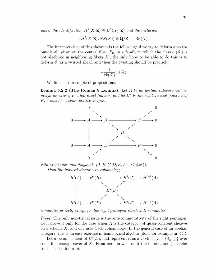
70

under the identification H2(X,Z) ∼= H2(X0,Z) and the inclusion

(H2(X,Z)/NS(X))⊗Q/Z → Br′(X).

The interpretation of this theorem is the following: if we try to deform a vectorbundle E0, given on the central fiber X0, in a family in which the class c1(E0) isnot algebraic in neighboring fibers Xt, the only hope to be able to do this is todeform E0 as a twisted sheaf, and then the twisting should be precisely

− 1

rk(E0)c1(E0).

We first need a couple of propositions:

Lemma 5.2.2 (The Roman 9 Lemma). Let A be an abelian category with e-nough injectives, F a left-exact functor, and let H i be the right derived functors ofF . Consider a commutative diagram

0 0ZZZ~

>

0 - A - B - C - 0ZZZ~

>

D

> Z

ZZ~

0 - A

wwwwwwwwww- E - F - 0

> Z

ZZ~

0 0

with exact rows and diagonals (A,B,C,D,E, F ∈ Ob(A )).Then the induced diagram in cohomology

H i(A) - H i(B) - H i(C) - H i+1(A)ZZZ~

>

H i(D)

> Z

ZZ~

H i(A)

wwwwwwwww- H i(E) - H i(F ) - H i+1(A)

wwwwwwwwwcommutes as well, except for the right pentagon which anti-commutes.

Proof. The only non-trivial issue is the anti-commutativity of the right pentagon;we’ll prove it only for the case when A is the category of quasi-coherent sheaveson a scheme X, and one uses Cech cohomology. In the general case of an abeliancategory, this is an easy exercise in homological algebra (done for example in [44]).

Let d be an element of H i(D), and represent it as a Cech cocycle dj0...ji oversome fine enough cover of X. From here on we’ll omit the indices, and just referto this collection as d.

71

Let c be the image of d under the natural map D → C (as Cech cocycles). Bypossibly refining the cover, one can lift c to a cochain b ∈ Ci(B). It is the failureof b to be a cocycle that gives the coboundary map H i(C)→ H i+1(A).

Let d′ be the cochain obtained by applying to b the map B → D. By thecommutativity of the triangle that contains B, C and D, d′ maps to c as well, sothat d− d′ maps to 0 in c, so d− d′ lifts to a cochain in E. Let this cochain be e.

Now e is a lift of f (where f is the image of d under the map D → F ): d′ comesfrom b, so it maps to 0 in F .

Computing, we have ∂e = ∂(d− d′) = −∂d′ = −∂b, which is what we needed.

Definition 5.2.3. Consider the two exact sequences on a space X

0→ O∗X →GL(n)→ PGL(n)→ 0

and

0→ Z/nZ→ SL(n)→ PGL(n)→ 0,

which we’ve already seen in Section 1.1 (as usual, we are using the etale or analytictopologies). For an element p of H1(X,PGL(n)), let a(p) and t(p) be the imagesof p under the two coboundary maps

H1(X,PGL(n))→ H2(X,O∗X)

and

H1(X,PGL(n))→ H2(X,Z/nZ),

respectively. We’ll call a(p) the analytic twisting class of p and t(p) the topologicaltwisting class of p. The first one belongs to Br′(X), and as such depends on thecomplex structure of X, while the second one is in H2(X,Z/nZ) and depends onlyon the topology of X.

If Y → X is a Pn−1-bundle over X, then the analytic and topological twist-ing classes of Y/X, t(Y/X) and a(Y/X), are the classes of the element p ofH1(X,PGL(n)) associated to the bundle Y → X.

Proposition 5.2.4. Let X be a scheme, E a rank n locally free sheaf on X andlet Y = Proj(E )→ X be the associated projective bundle. Then

t1(Y/X) = −c1(E ) mod n.

(Here, and in the sequel, by reducing mod n we mean applying the natural mapH2(X,Z)→ H2(X,Z/nZ)).

72

Proof. Consider the commutative diagram with exact rows and diagonals

0 0QQQs

3

0 - Z/nZ - SL(n) - PGL(n) - 0QQQs

3

GL(n)

3 Q

QQdets

0 - Z/nZ

wwwwwwwww- O∗X

·n- O∗X - 0

3 Q

QQs

0 0

and apply the Roman 9 lemma for i = 1. We get the anti-commutative diagram

H1(X,PGL(n))t1 - H2(X,Z/nZ)

>

H1(X,GL(n))ZZZdet~H1(X,O∗X)

c1 mod n- H2(X,Z/nZ)

wwwwwwwwwwhich is exactly what we need.

Proposition 5.2.5. For any integer n consider the following two natural maps:one, the map ϕ : H2(X,Z/nZ)→ Br′(X) obtained from the short exact sequence

0→ Z/nZ→ O∗X·n→ O∗X → 0.

The other one is mapping H2(X,Z) to Br′(X) by taking x ∈ H2(X,Z) to 1nx ∈

H2(X,Z)⊗Q/Z, which naturally maps to Br′(X).Then, the following diagram commutes:

H2(X,Z)mod n

- H2(X,Z/nZ)

@@@x 7→ 1

nx R

ϕBr′(X).

Furthermore, if Y → X is a Pn−1-bundle over X, and t(Y/X) and a(Y/X) arethe topological and analytic twisting classes associated to it, then we have

ϕ(t(Y/X)) = a(Y/X).

73

Proof. Trivial chase through the definitions. The last statement follows from thecommutativity of the diagram

H1(X,PGL(n))t- H2(X,Z/nZ)

H1(X,PGL(n))

wwwwwa- Br′(X),

?

which is deduced from the map of short exact sequences

0 - Z/nZ - SL(n) - PGL(n) - 0

0 - O∗X

?- GL(n)

?- PGL(n)

wwwww- 0.

Proof. (of Theorem 5.2.1) Let n = rk(E ), and consider the projective bundleassociated to E , Y = Proj(E ) → X. As such, it has an associated topologicaltwisting class, t = t(Y/X) ∈ H2(X,Z/nZ), for which we have ϕ(t) = α, whereϕ is the map from the previous proposition. Since the topological twisting classis natural and is a topological invariant, we must have t|Xs = t(Ys/Xs) for everys ∈ S. But on X0, we must have t|X0 = −c1(E0) mod n by Proposition 5.2.4. Sincethe map ϕ is compatible with restriction, we have

α = ϕ(t) = ϕ(t|X0) = ϕ(−c1(E0) mod n) = − 1

nc1(E0).

Remark 5.2.6. In particular, this shows that on Xs we must have

α|Xs = − 1

nc1(E0)

as well.

5.3 Identifying the Obstruction

In this section we compute, for a moduli problem on a K3 surface, the obstruction αto the existence of a universal sheaf (Definition 5.1.8), in terms of the cohomologicalFourier-Mukai transform described in Definition 5.1.9.

The setup is, as before, an algebraic K3 surface X, with a fixed polarization P,and v a primitive, isotropic vector in H1,1(X)∩H(X,Z), such that the moduli spaceof semistable sheaves of Mukai vector v, M(v), is non-empty and does not containany properly semistable points. Then, according to Theorem 5.1.6, M = M(v) is

74

a K3 surface, and choosing a quasi-universal sheaf U we obtain a Fourier-Mukaitransform

ϕU ∨

X→M : H(X,Q)→ H(M,Q)

(which depends on U ).There is a natural element α ∈ Br(M) which expresses the obstruction to the

existence of a universal sheaf on X ×M . The following theorem gives a preciseidentification of α in terms of the initial data X and v.

Theorem 5.3.1. Let u ∈ H(X,Z) be any vector such that (u, v) = 1 mod n,(where n is the one defined in Theorem 5.1.12) and let w = ϕU ∨

X→M(u). Denote byw2 the H2(M,Q) component of w, and let w be the element of Br(M) that is theimage of w2 under the composite homomorphism

H2(M,Q)→ H2(M,Q/Z)→ H2(M,Q/Z)/(NS(X)⊗Q/Z) = Br(M).

Then w is the obstruction to the existence of a universal sheaf on X × M , asdescribed in Definition 5.1.8.

Remark 5.3.2. Since H(X,Z) is a unimodular lattice, one can always find a vectoru satisfying (u, v) = 1 mod n, so that one can always compute the obstructionα = w using this theorem.

Proof. Let’s start off by analyzing the Fourier-Mukai transform when the moduliproblem is in fact fine, but we are using a quasi-universal sheaf instead of theuniversal sheaf.

So assume that we are in the above setup, with n = 1, and therefore thereexists a universal sheaf E on X ×M . If OX(1) is an ample line bundle on X, andk is large enough, then

V = ΦE∨

X→M(OX(−k))[2]

is a locally free sheaf on M . Indeed, this is a relative version of the fact that on asmooth, projective scheme of dimension r, we have

Extr−i(F (k), ω) = H i(F (k)) = 0

for any coherent sheaf F , i > 0, and large enough k. So let k be large enough tohave V locally free. We are interested in the quasi-universal sheaf U = E ⊗π∗MV ,of similitude rk(V ).

It is important to note that we have

v(V ) = v(ΦE∨

X→M(OX(−k))[2])

= v(ΦE∨

X→M(OX(−k)))

= ϕE∨

X→M(v(OX(−k))),

75

and therefore

rk(V ) = (v(V ), (0, 0, ωM))

= (ϕE∨

X→M(v(OX(−k))), ϕE∨

X→M(v))

= (v(OX(−k)), v),

because the Fourier-Mukai transform is an isometry.Let F be a line bundle on X, anti-ample enough so that

G = ΦU ∨

X→M(F )[2]

is a locally free sheaf on M . We have

G = ΦE∨

X→M(F )[2]⊗ V

by the projection formula, so that

c1(G ) = rk(V ) · c1(ΦE∨

X→M(F )[2]) + rk(ΦE∨

X→M(F )[2]) · c1(V ).

Butrk(ΦE∨

X→M(F )[2]) = (v(F ), v)

by a computation identical to the one above, and therefore

ϕU ∨

X→M(v(F ))2 =1

rk(V )c1(G )

=(v(F ), v)

rk(V )c1(V ) + integral part,

where the subscript 2 denotes the H2(M,Q)-part.We now return to the case when n 6= 1, and we start by proving that w is

independent of the choice of U and u. If U and U ′ are two quasi-universalsheaves, then there exists another quasi-universal sheaf U ′′ and vector bundles Fand F ′ on M such that

U ′′ ∼= U ⊗ π∗MF ∼= U ′ ⊗ π∗MF ′,

(remark before Theorem A.5 in [33]), so it is enough to prove that w is the samewhen using U and U ′ = U ⊗π∗MF (for some vector bundle F on M) in computingthe Fourier-Mukai transform.

A standard calculation shows that

ϕU ′∨

X→M(u)2 = ϕU ∨

X→M(u)2 +(u, v)

rk Fc1(F ),

(see [25, Definition 6.1.12], or the previous computations), and therefore

ϕU ′∨

X→M(u)2 = ϕU ∨

X→M(u)2

76

in H2(M,Q)/(NS(M)⊗Q). Thus w is independent of the choice of U , and hencefrom now on we’ll omit the superscript U ∨ in ϕU ∨

X→M .Let u, u′ ∈ H(X,Z) be such that

(u, v) = (u′, v) = 1 mod n.

Then (u − u′, v) is divisible by n, and since n is the greatest common divisor of(t, v) where t runs over all algebraic vectors in H(M,Z) we conclude that thereexists a t ∈ H(M,Z), algebraic, and such that (u − u′ − t, v) = 0. Using [33,Theorem 1.5], we conclude that

ϕ2(u)− ϕ2(u′)− ϕ2(t)

is integral. Also, since t was algebraic, ϕ(t) is also algebraic; therefore, ϕ2(u) andϕ2(u′) must be equal in

H(M,Q)/((H1,1(M) ∩ H(M,Q)) + H(M,Z)),

which is Br(M). Thus w is also independent of the choice of u.From here on proceed as in the proof of (2) and (3) of Theorem 1.5 in [33] (pp.

385-386). Fix an ample line bundle OX(1) on X, let l be its class in H2(X,Z),and let v2 be the projection of v onto H2(X,Z). Let T0 be the moduli space ofK3 surfaces X ′ with an isometric marking i : H2(X ′,Z) → H2(X,Z) such thati∗v2 and i∗l are algebraic on X ′, and i∗OX(1) is ample. T0 contains a point 0corresponding to (X, id) and is of dimension 18 or 19 according to whether l andv2 are linearly independent in H2(X,Z) or not. Over an analytic neighborhood ofthe origin in T0 we have a smooth family X → T0. On each fiber Xt (t ∈ T0),fix the polarization given by i∗OX(1), and consider the moduli space Mt of stablesheaves on Xt, having Mukai vector i∗v, with respect to this polarization.

The spaces Mt form a flat family M → T0, which is smooth over some analyticneighborhood of the origin in T0, and by restricting T0 further we can also assumethat Mt is compact for all t ∈ T0. On the other hand, since the set of points t ∈ T0

for which Mt is a fine moduli space is dense in T0, we can assume that there exists1 ∈ T0 for which M1 is the fine moduli space of semistable sheaves on X1. (Mt wastaken to be the moduli space of stable sheaves on Xt; however, the compactnessassumption on Mt implies that there are no properly semistable points in Mt, sothat the notions of semistable and stable coincide.)

Using Theorems 3.3.2 and 3.3.4, we get an α ∈ Br(M ) and an α-twisteduniversal sheaf E on X ×T0 M . By restricting T0 even further (to an open set ofa component of T0), we can assume T0 is smooth, and Br(T0) = 0. Using this lastproperty, we can find a relatively ample sheaf OX (1) on X , which restricts to thefixed polarization i∗OX(1) on each fiber of X .

As before, consider

V = RπM ,∗(Lπ∗X O(−k)

L⊗ E ∨)[2]

77

for some k 0. By the same argument as before, V consists of a single α−1-twisted locally free sheaf. (The twisting is by α−1 because we have dualized E .)We are thus in the situation studied in the previous section: we have a smoothfamily M → T0 over a smooth base, an element α ∈ Br(M ) such that over M1 wehave α−1|M1 = 0, and an α−1-lffr V over M . Under these circumstances, we canapply Theorem 5.2.1 and conclude that

α−1 = − 1

rk(V1)c1(V1),

and hence

α =1

rk(V1)c1(V1),

where V1 is some gluing of V |M1 to a global locally free sheaf (under the identifi-cations discussed in Section 5.2).

As a quasi-universal sheaf on X ×T0 M we can take

U = E ⊗ π∗MV ,

which naturally glues to a sheaf on X ×T0 M . Form here on this will be theuniversal sheaf we’ll be using for defining the Fourier-Mukai transforms.

Of course, as an element of Br(M1), α is zero (being algebraic), as expectedfrom the fact that the moduli problem is fine at t = 1. However, the right handside of the equality

α =1

rk(V1)c1(V1),

is defined solely in topological terms, and is therefore constant in the family M →T0. Also, since U is defined in the whole family, ϕU ∨

Xt→Mt(u) is constant as a

function of t ∈ T0, for any u ∈ H(X,Z). Therefore, if we prove that

ϕU ∨

X1→M1(u)2 =

(u, v)

rk(V1)c1(V1) + integral part,

for some u ∈ H(X1,Z) with (u, v) = 1 mod n, then we can conclude that thesame equality holds at t = 0, after identifying H(M0,Z) ∼= H(M1,Z). The righthand side of the above equality reduces to (u, v)α in Br(M0), therefore using thefact that α is n-torsion (Theorem 5.1.12) we get

w = ϕU ∨

X1→M1(u)2 = (u, v)α = α.

But let’s now look at what is happening over t = 1 ∈ T0; we are precisely inthe situation discussed in the beginning of the proof: the moduli problem is fine,and we have a polarization OX1(1) of which we take a sufficiently negative multipleand apply the Fourier-Mukai transform to get V1 on M1. Therefore, if we considera line bundle F on X1, which is sufficiently anti-ample, we have

ϕU ∨

X1→M1(v(F ))2 =

(v(F ), v)

rk(V1)c1(V1) + integral part.

78

All we need to do now is show that we can find an F as above for which (v(F ), v) =1 mod n. Indeed, we can then take u = v(F ) (using the fact the we have thefreedom of choosing u as long as (u, v) = 1 mod n) and get

ϕU ∨

X1→M1(u)2 = ϕU ∨

X1→M1(v(F ))2

=(v(F ), v)

rk(V1)c1(V1) + integral part

=(u, v)

rk(V1)c1(V1) + integral part,

which is what we want.Since we assume that n = 1 at t = 1 we can find a line bundle F on X1 with

c1(F ) = d such that gcd(v0, v2.d, v4) = 1 (where v = (v0, v2, v4)). Since n dividesv0 and v4, we must have gcd(v2.d, n) = 1. By possibly replacing F by some tensorpower of itself, we can assume (v2.d) = 1 mod n. Then we have

v(F ).v = v2.d− v4 − v0 − v0(d.d) = 1 mod n,

as desired. Twisting F by OX1(−k) for k large enough, we get the F we werelooking for, thus finishing the proof. (Note that twisting by O(−k) does not change(v(F ), v) mod n, because (c1(OX1(1)).v2) must be divisible by n, since it equals(c1(OX0(1)).v2).)

5.4 The Map on Brauer Groups

We have seen in the previous section that we can identify the obstruction α solelyin terms of the Fourier-Mukai transform. In this section we prove that there is infact a map between the Brauer groups of X and of M , whose kernel is generatedby α.

Lemma 5.4.1. Let M be a K3 surface, and let TM be the transcendental latticeof M , i.e. the orthogonal lattice to NS(M) inside H2(M,Z) (endowed with theintersection pairing). Then there is a natural isomorphism

Br(M) = T ∨M ⊗Z Q/Z,

where T ∨M is the dual lattice to TM .

Proof. Consider the exact sequence of Proposition 1.1.3,

0→ NS(M)⊗Q/Z→ H2(M,Q/Z)→ Br(M)→ 0,

(note that for a K3 M we have NS(M) = Pic(M)); using the universal coefficienttheorem, we also know that

H2(M,Q/Z) = H2(M,Z)⊗Q/Z,

79

and thereforeBr(M) = (H2(M,Z)/NS(M))⊗Q/Z.

Now consider the map

p : H2(M,Z)→ T ∨M

given by

p(v)(w) = (v, w)

for w ∈ TM . It is obviously a linear map, it is surjective (because H2(M,Z) isunimodular) and its kernel consists of all v ∈ H2(M,Z) such that (v, w) = 0 forall w ∈ TM , which is T⊥M . Since NS(M) is a primitive sublattice in H2(M,Z), wehave

T⊥M = (NS(M)⊥)⊥ = NS(M),

and therefore we conclude that

T ∨M = H2(M,Z)/NS(M),

thus obtaining the result of the lemma.

Lemma 5.4.2. Let H be a unimodular lattice, let N be a primitive sublattice inH, and let n be a fixed integer. Define Nn to be the sublattice of N consisting of allx ∈ N such that (x, y) is divisible by n for all y ∈ N . Also, let T = N⊥, and let Tnbe defined just as Nn. Then there is a natural group isomorphism Nn/nN ∼= Tn/nTdefined by sending an element v ∈ Nn/nN to the unique element λ of Tn/nT suchthat v − λ is divisible by n inside H.

Proof. Begin by proving that for every v ∈ Nn there exists a λ ∈ Tn such thatv − λ is divisible by n. The idea is from [32]: consider the functional

1

nv∨ =

1

n(v, ·) ∈ N∨

(it takes integer values because v ∈ Nn). Since N is a primitive sublattice inthe unimodular lattice H, there exists w ∈ H such that w∨|N = 1

nv∨. Thus

(v − nw, x) = 0 for all x ∈ N , and thus λ = v − nw ∈ T . Obviously, we havev − λ divisible by n inside H (equaling nw). The fact that λ is in fact in Tn isimmediate:

(λ, y) = (λ− v, y) = −n(w, y)

for any y ∈ T .It is obvious that the map is well-defined, bijective, and a group homomorphism,

so we’re set.

80

Theorem 5.4.3. Let X be a K3 surface, v ∈ H1,1(X) ∩ H(X,Z) a primitiveisotropic Mukai vector, and assume that the moduli space M = M(v) of semistablesheaves on X of Mukai vector v is non-empty and does not contain any properlysemistable points, so that M is again a K3 surface by Theorem 5.1.6. Then thereis a natural exact sequence

0→ Z/nZ→ Br(M)→ Br(X)→ 0,

(where n is the one defined in Theorem 5.1.12), induced by the map ϕ : TX → TMof the same theorem. The cyclic kernel of the map Br(M) → Br(X) is generatedby the obstruction α ∈ Br(M) to the existence of a universal sheaf on X ×M , andthis particular generator of the kernel is in fact singled out by the construction ofthe exact sequence.

Remark 5.4.4. The last statement of the proposition should be interpreted as fol-lows: the exact sequence between the Brauer groups is fully determined by justknowing the cyclic subgroup 〈v〉 of H1,1(X,Z/nZ) generated by v. However, havingsingled out a particular generator v of this subgroup, this singles out a particulargenerator α of the kernel of the map Br(M) → Br(X), and it is this particulargenerator that is the obstruction to the existence of a universal sheaf on X ×Mthat is asserted in Definition 5.1.8. See the actual proof for more details.

Proof. Using Lemma 5.4.2, we obtain a natural correspondence between elementsof H1,1(X,Z)n/nH

1,1(X,Z) and elements of TX,n/nTX . Since v ∈ H1,1(X,Z)n, weget an element λ ∈ TX,n such that v − λ is divisible by n in H(X,Z). (Here, λ isuniquely defined by v up to an n-multiple of TX .)

Consider the exact sequence

0→ TXϕ−→ TM → Z/nZ→ 0

from Theorem 5.1.12, where ϕ is a Fourier-Mukai transform defined by means ofquasi-universal sheaf (it does not depend on this choice). The cokernel of the firstmap is generated by the element µ = 1

nϕ(λ). Dualizing, we get

0→ T ∨M → T ∨X → Z/nZ = Ext1Z(Z/nZ,Z)→ 0,

where the last map isψ ∈ T ∨X 7→ ψ(λ) mod n.

Tensoring this exact sequence with Q/Z we get

0→ Z/nZ = TorZ1 (Z/nZ,Z)→ T ∨M ⊗Q/Z→ T ∨X ⊗Q/Z→ 0,

or, in view of Lemma 5.4.1,

0→ Z/nZ→ Br(M)→ Br(X)→ 0.

81

In order to identify the kernel, note that the map ϕ becomes invertible whentensored with Q, and the same holds also for ϕ∨. If ψ ∈ T ∨X is such that ψ(λ) =1 mod n, then ψ′ = ψ(ϕ⊗Q)−1 is an element of T ∨M⊗Q whose image in T ∨M⊗Q/Zgenerates the kernel. Indeed, its image in T ∨X⊗Q is ψ, which is integral (and hencebecomes zero in T ∨X ⊗ Q/Z), so it belongs to the kernel. Since ψ generates thecokernel of the map T ∨M → T ∨X , ψ′ generates the kernel of T ∨M ⊗Q/Z→ T ∨X⊗Q/Z.

It is easy to see that all these constructions are natural, and that having chosena particular generator µ for the cokernel of TX → TM , we have singled out agenerator of the kernel of Br(M)→ Br(X).

Now consider the result of Theorem 5.3.1: it states that in order to obtain α,we have to find u ∈ H(X,Z) such that (u, v) = 1 mod n, and consider the image

α = ϕ(u) ∈ Br(M).

Tracing through the identifications of Br(M) with T ∨M ⊗Q/Z, we find that ϕ(u) ∈Br(M) corresponds to the functional ψ′ ∈ T ∨M ⊗Q/Z given by

ψ′( · ) = (ϕ(u), · ),

where ϕ(u) is now viewed as an element of H(M,Q). But it is easy to see that

ψ′(ϕ(λ)) = (ϕ(u), ϕ(λ)) = (u, λ) = 1 mod n,

the last equality following from the fact that v − λ is divisible by n by the con-struction of λ, and (u, v) = 1 mod n.

Thereforeψ( · ) = ψ′ ϕ( · ) = (ϕ(u), ϕ( · )) = (u, · )

is an integral functional on TX , satisfying ψ(λ) = 1 mod n, and thus ψ′ is thedistinguished generator of the kernel of the map

T ∨M ⊗Q/Z→ T ∨X ⊗Q/Z.

We conclude that α, the obstruction to the existence of a universal sheaf on X ×M , is precisely the distinguished generator of the kernel of the map Br(M) →Br(X).

Remark 5.4.5. This result should be contrasted with [11, 5.3.5], where the authorsobserve that in the case of an elliptically fibered K3 X, Br(X) = Br(J), where J isthe relative Jacobian. Of course, J can be viewed as a moduli space of semistablesheaves on X (Chapter 4), so that one should in fact get

0→ Z/nZ→ Br(J)→ Br(X)→ 0,

with the kernel generated by α ∈ Br(J) which is the obstruction to the existenceof a universal sheaf on X × J , which coincides with the element α ∈XS(J) thatrepresents X. The explanation for this apparent mismatch is the following: Br(X)

82

and Br(J) are isomorphic, as abstract groups. Indeed, they are isomorphic toT ∨X ⊗ Q/Z and T ∨J ⊗ Q/Z, respectively, and TX is isomorphic to TJ as abstractgroups. However, if one takes into account the lattice structure on TX and TJ , oneobtains the more precise formulation of Theorem 5.4.3.

Remark 5.4.6. Identifying Br(M) with T ∨M ⊗ Q/Z, we can view any α ∈ Br(M)as a functional on TM , with values in Q/Z. Theorem 5.4.3 states that TX isHodge isometric (via the Fourier-Mukai transform) to Ker(α), viewed as a Hodgesublattice of TM . The striking thing about this is the following: if one takes αk (wekeep the multiplicative notation for the operation in Br(M)) for gcd(k, ord(α)) =1, then obviously Ker(αk) = Ker(α). Thus, if we have X and X ′ K3 surfaces,and v ∈ H1,1(X,Z), v′ ∈ H1,1(X ′,Z) such that MX(v) = M = MX′(v

′), andObs(M, v) = α, Obs(M ′, v′) = αk, then TX is Hodge isometric to TX′ . This willbe used in the following section.

5.5 Relationship to Derived Categories

Whenever one deals with a moduli problem of semistable sheaves on a K3 X, andthe moduli space M is 2-dimensional and has no properly semistable points, thenone gets an equivalence of derived categories between some derived category oftwisted sheaves on M , and the derived category of (usual) coherent sheaves on X.This is the content of the following theorem.

Theorem 5.5.1. Let X be a K3 surface, let v ∈ H1,1(X,Z) be a primitive,isotropic Mukai vector, and assume that there is a polarization on X such thatthe moduli space M = MX(v) of semistable sheaves with Mukai vector v is non-empty and does not contain any properly semistable points. Let α = Obs(X, v).Then we have

Dbcoh(X) ∼= Db

coh(M,α−1).

Proof. Using Theorem 3.3.2 we conclude that there exists a π∗Mα-twisted universalsheaf U on X ×M . Therefore we can consider the integral functor

F = ΦUM→X : Db

coh(M,α−1)→ Dbcoh(X)

defined by U , and in order to check that F is an equivalence, all we have to do ischeck that the conditions of Theorem 3.2.1 are satisfied.

For a point [F ] ∈ M that corresponds to a stable sheaf F on X with Mukaivector v, we have F (O[F ]) = F , from the very definition of a universal sheaf. Thusthe conditions of Theorem 3.2.1 can be restated as:

1. if F 6= G , Exti(F ,G ) = 0 for all i;

2. Hom(F ,F ) = C, and Exti(F ,F ) = 0 for all i < 0 or i > 2;

3. F ⊗ ωX ∼= F ;

83

for all F , G stable sheaves on X with Mukai vector v.Since X is smooth of dimension 2, Exti(F ,G ) = 0 for i < 0 or i > 2 anyway.

Since F and G are stable, Hom(F ,G ) = 0 if F 6= G . Therefore Ext2(F ,G ) = 0by Serre duality (use the fact that ωX is trivial). Since

χ(F ,G ) = (v(F ), v(G )) = (v, v) = 0

by Lemma 3.1.7, we conclude that Ext1(F ,G ) = 0 as well. Hom(F ,F ) = Cbecause a stable sheaf is simple. Finally, the last condition holds automaticallybecause ωX is trivial.

As an application of this we prove the following:

Theorem 5.5.2. Let M be a K3 surface, let α ∈ Br(M), and let k ∈ Z be suchthat gcd(k, ord(α)) = 1. Assume that there exist K3 surfaces X and X ′, and Mukaivectors v ∈ H1,1(X,Z), v′ ∈ H1,1(X ′,Z) such that we have isomorphisms

M ∼= MX(v) ∼= MX′(v′),

and such that under these isomorphisms, Obs(X, v)−1 = α and Obs(X ′, v′)−1 = αk.Then we have

Dbcoh(M,α) ∼= Db

coh(M,αk).

Proof. We have seen (Remark 5.4.6) that under these assumptions TX is Hodgeisometric to TX′ . Orlov’s theorem (Theorem 5.1.14) then tells us that

Dbcoh(X) ∼= Db

coh(X ′).

But Theorem 5.5.1 shows that Dbcoh(M,α) ∼= Db

coh(X) and Dbcoh(M,αk) ∼=

Dbcoh(X ′), and thus

Dbcoh(M,α) ∼= Db

coh(M,αk).

It is tempting (especially in view of the results of Chapter 6) to conjecture thatthe conclusion of the previous theorem holds more generally:

Conjecture 5.5.3. For any K3 surface M , and any twisting α ∈ Br(M), we have

Dbcoh(M,α) ∼= Db

coh(M,αk)

for any k with gcd(k, ord(α)) = 1.

The difficulty in proving such a theorem would lie on one hand in the fact thatif one takes TX = Ker(α), then TX may not be embeddable in the K3 lattice LK3.Even if one assumes this embeddability condition, there are problems with findingthe Mukai vector v.

84

Remark 5.5.4. There is one more thing to note here: having started with M andα, an easy way to find X would be to consider Db

coh(M,α), and take X to bethe “spectrum” of this derived category (see [39] for details on the spectrum of atriangulated category and related topics). This would work, of course, only if Xexisted, and by Theorem 5.4.3 we know that in this case TX = Ker(α). This wouldmean in particular that Ker(α) can be primitively embedded in LK3. This doesnot in general hold, but Theorem 5.4.3 gives us anyway a candidate for TX ! Theconclusion of this is that Db

coh(M,α) should be viewed as a derived category of a“virtual” K3 X, where X itself might not necessarily exist, but it makes sense tospeak of its transcendental lattice.

Another interesting conjecture which relates to these topics is the following:

Conjecture 5.5.5. If X and X ′ are K3 surfaces with Dbcoh(X) ∼= Db

coh(X ′), thenTheorem 5.4.3 gives us a natural isomorphism ϕ : Br(X) ∼= Br(X ′). Is it then thecase that Db

coh(X,α) ∼= Dbcoh(X ′, ϕ(α))?

Chapter 6

Elliptic Calabi-Yau Threefolds

In this chapter we pursue further the results of Chapter 4, to the case of someelliptic fibrations with singular fibers. We are mainly interested in elliptic Calabi-Yau threefolds, and we only consider a number of generic examples here. By“generic” we mean that the singularities of the fibers are the simplest possible tostill get a Calabi-Yau: the discriminant locus ∆ is a curve with only nodes andcusps as singularities, and the curve over the generic point of ∆ is a rational curvewith one node (I1). (See Section 6.1 for details on this topic.)

We provide three examples of such fibrations in Section 6.2. The first one isfolklore, but the second and third ones are, to the best of my knowledge, new.

Given a fibration with the above properties, our first concern is understandingthe relative Jacobian, which is defined as a relative moduli space (Section 6.4).In order to do this, we need to understand moduli spaces of semistable sheaveson the fibers of X, and we do this in Section 6.3. Having done that, we goon to study the relative Jacobian in Section 6.4. We note here an interestingphenomenon: although the space X we start with is smooth, the relative Jacobianhas singularities. These singularities can not be removed without losing the Calabi-Yau property (J has trivial canonical bundle, but a small – or crepant – resolutiondoes not exist in general).

The existence of these singularities would seem to prevent us from finding anequivalence of derived categories (since derived categories “detect smoothness”, aswell as triviality of canonical bundle), but by working in the analytic category weare able to bypass this problem. Indeed, in this category we find a small resolutionJ of the singularities of J , and we are able to show that there exists a twisted“pseudo-universal” sheaf on X ×S J (where S is the base of the fibrations). Thistwisted pseudo-universal sheaf is equal to the usual twisted universal sheaf overthe stable part of J (which equals the stable part of J), but also parametrizes someof the semistable sheaves on X, over the properly semistable part of J (which isthe resolution of the singular, semistable points of J). Using this pseudo-universalsheaf, we can define an integral transform, which turns out to be an equivalence.This is done in Section 6.5.

We then note, in Section 6.6 another occurrence of the same surprising phe-

85

86

nomenon observed in Section 5.5: on J , we get an equivalence of derived categories

Dbcoh(J , α) ∼= Db

coh(J , αk),

where α ∈ Br(J) is the twisting associated to X via Ogg-Shafarevich theory, andgcd(k, ord(α)) = 1.

In the next section we discuss the relationship of derived categories and theTorelli problem for Calabi-Yau threefolds. We show that Calabi-Yau threefoldswith equivalent derived categories have the same Hodge data, and hence theyprovide a counterexample to the generalization of Torelli from K3 surfaces. Inparticular, we provide such an example based on the elliptic Calabi-Yau’s studiedin Section 6.2.

We finish this chapter with a section on the relationship of these exampleswith the example of Vafa-Witten ([43]) and Aspinwall-Morrison-Gross ([1]). Wegive a quick overview of their example, and suggest a possible explanation for theoccurrence of stable singularities in string theory.

6.1 Generic Elliptic Calabi-Yau Threefolds

In this section we define the objects of study in this chapter: a certain classof elliptic Calabi-Yau three-folds, in which we have very good control over thedegenerations of the elliptic fibers. The results in this section could probably beeasily generalized to arbitrary elliptic fibrations without multiple fibers, but sincethe results here are intended only to give life to some large class of examples, we’lllimit ourselves to this sufficiently general situation.

Recall the definition of a Calabi-Yau threefold:

Definition 6.1.1. A smooth, projective algebraic variety or analytic space X iscalled a Calabi-Yau threefold if it has (complex) dimension 3, and if it satisfiesKX = 0 and H1(X,OX) = 0. (Here, and in the future, KX denotes the canonicaldivisor of X.)

We will be focused on studying the case of complex threefolds, in which case theHodge structure of X will come into play. It is described by the Hodge diamond

10 0

0 h2,2 01 h2,1 h1,2 1

0 h1,1 00 0

1.

Of course, h1,1 = h2,2, and h2,1 = h1,2.The following definitions are from [13]:

87

Definition 6.1.2. A projective morphism f : X → S of algebraic varieties oranalytic spaces is called an elliptic fibration if its generic fiber E is a regular curveof genus one and all fibers are geometrically connected. If X is a Calabi-Yauthreefold, then f is called an elliptic Calabi-Yau threefold.

Remark 6.1.3. Most of the time we’ll abuse the notation, by saying “let X be anelliptic Calabi-Yau threefold.” By this we mean “let X be a Calabi-Yau threefold,and let f : X → S be an elliptic fibration on X.”

Definition 6.1.4. Let f : X → S be an elliptic fibration. The locus ∆ ⊆ S ofpoints s ∈ S such that f is not smooth at some point x ∈ X with f(x) = s, iscalled the discriminant locus of f . It is a Zariski closed subset of S. The closedsubset of ∆

∆m = s ∈ S | f is not smooth at any x ∈ f−1(s)

is called the multiple locus of f . A fiber over a point s ∈ ∆m is called a multiplefiber.

We will only be interested in studying elliptic fibrations without multiple fibers,so from now on we make the assumption that ∆m = ∅.

Definition 6.1.5. A section (resp. a rational section) of an elliptic fibration f :X → S is a closed subscheme Y of X for which the restriction of f to Y is anisomorphism (resp. a birational morphism). A degree n multisection (or an n-section) is a closed subscheme Y of X such that the restriction of f to Y is a finitemorphism of degree n. A rational degree n multisection is a closed subscheme Yof X such that the restriction of f to Y is generically finite of degree n.

When working in the algebraic category, it is well-known that any elliptic fibra-tion has a rational multisection. In the analytic category this does not necessarilyhold true any more, but we will always assume not only the existence of a rationalmultisection, but even more: that the elliptic fibrations under consideration havemultisections (not only rational).

Definition 6.1.6. For the rest of this chapter, define a generic elliptic Calabi-Yauthreefold to be an elliptic threefold f : X → S, with X and S smooth algebraicvarieties over C or complex manifolds, X Calabi-Yau, and satisfying the followingextra properties:

1. f is flat (i.e. all fibers are 1-dimensional);

2. f does not have any multiple fibers;

3. f admits a multisection;

4. the discriminant locus ∆ is a reduced, irreducible curve in S, having onlynodes and cusps as singularities;

88

5. the fiber over a general point of ∆ is a rational curve with one node.

Remark 6.1.7. The reason for calling such an elliptic fibration “generic” is the factthat, in many families of elliptic Calabi-Yau threefolds, these properties are sharedby the general members of the family. See the examples in Section 6.2 for moredetails.

From here on we fix a generic elliptic Calabi-Yau threefold f : X → S, whosestructure we want to investigate.

Theorem 6.1.8. Locally, in the etale or analytic topology, f has a section.

Proof. This is an immediate consequence of the fact that f has no multiple fibers.

Theorem 6.1.9. The fibers of f are as follows:

(0) over s ∈ S \∆, Xs is a smooth elliptic curve;

(I1) over a smooth point s of ∆, Xs is a rational curve with one node;

(I2) over a node s of ∆, Xs is a reducible curve of type I2, i.e. two smooth P1’smeeting transversely at two points;

(II) over a cusp s of ∆, Xs is a rational curve with one cusp.

Furthermore, in the case of the I2 fiber, each component C of the fiber has normalbundle

NC/X∼= OC(−1)⊕ OC(−1).

Proof. See [31].

Remark 6.1.10. Let s ∈ ∆ be a node of the discriminant locus, and let U be aneighborhood of s such that XU → U has a section. Fix such a section. Then,according to [13, 2.3] and [35, 2.1], there exists a birational morphism π : XU → X ′

of schemes over U , which contracts the component of the I2 fiber which is not metby the chosen section of XU → U , and such that X ′ → U is a Weierstrass model(see, for example, [13] for a review of the theory of Weierstrass models). Most ofthe work in the next few sections will consist of understanding this map better,from the point of view of moduli spaces of semistable sheaves.

6.2 Examples

In this section we give three examples of generic elliptic Calabi-Yau threefolds.The first example is mainly folklore, while the last two examples are original, andthey are used in Section 6.7 to construct possible counterexamples to the Torelliproblem.

89

Example 6.2.1. We’ve already seen a first example of a generic elliptic Calabi-Yau threefold in Example 4.1.2. Indeed, the only thing we need to check is thatthe map f : X → P2 satisfies the conditions for being a generic elliptic threefold.The facts that the fibers are 1-dimensional (so that f is flat), there are no multiplefibers, and f admits a multisection are immediate. The discriminant locus is areduced curve of degree 36, with 216 cusps and 189 nodes. (This can be checkeddirectly using the software package Macaulay [28], or by using Euler characteristiccomputations.) As we have seen before, this elliptic fibration has n = 3 (smallestdegree of a multi-section) and the only twisted powers of it (as in Section 4.5) areits relative Jacobian and itself.

Example 6.2.2. In this example we will construct a generic elliptic Calabi-Yauthreefold X → P2. The ambient space under consideration is P2 × P4, withcoordinates x0, . . . , x2, y0, . . . , y4. Let M be a generic 5×5 skew-symmetric matrixwhose (i, j)-th entry is a polynomial of bi-degree (1 − δj5, 1) (in other words, thebi-degree is (1, 1) everywhere except the last row and column, where it is (0, 1)).According to [15, 0.1], the 4× 4 Pfaffians of this matrix define a degeneracy locusX, which has a symmetric locally free resolution

0→ L → Eϕ−→ E ∨(L )→ OP2×P4 → OX → 0,

where

L = ωP2×P4 = O(−3,−5),

E =5⊕i=1

O(ai,−3),

(ai) = (−2,−2,−2,−2,−1),

and the map ϕ is given by the matrix M . Then it can be easily checked using theresults in [15] that X is a smooth Calabi-Yau three-fold.

The projection of X to P2 is surjective and flat, and the fibers are degree 5curves in P4 given by Pfaffians of a skew-symmetric 5 × 5 matrix. Therefore thefibers are (generically) elliptic curves, and it can be checked by computer that thisexhibits X → P2 as a generic elliptic fibration.

The projection of X to P4 maps to a quintic threefold Q in P4, contracting 52lines and a conic, to 53 ordinary double points in Q. It can now be checked usingstandard techniques that the Picard number of Q (and therefore that of X) is 2.Let D and H be pull-backs of hyperplane sections from P2 and P4, respectively.It is easy to compute intersection numbers. They are:

D3 = 0, D2H = 5, DH2 = 9, H3 = 5.

Since D2H and DH2 are coprime, D and H must be primitive in NS(X), soOX(D) and OX(H) generate Pic(X). If F = D2 is a fiber of X → P2, then wehave DF = 0 and HF = 5, so we conclude that n = 5 (smallest degree of a

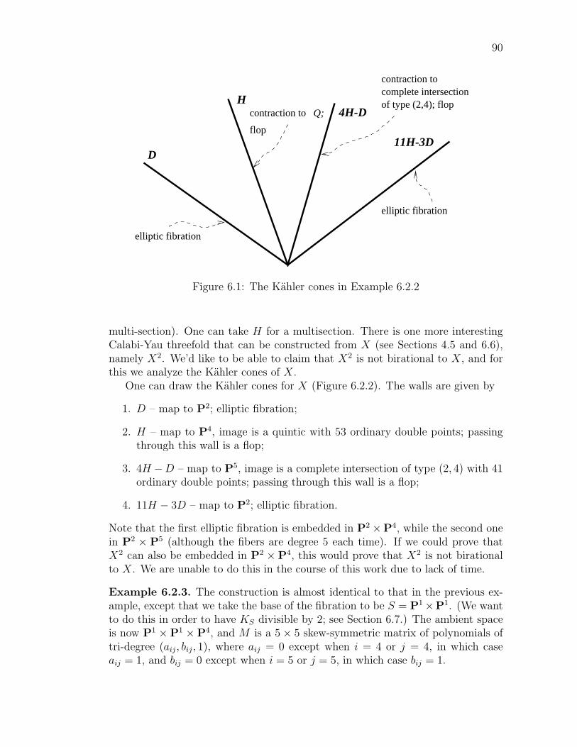
90

D

H4H-D

elliptic fibration

contraction to

flop

contraction tocomplete intersectionof type (2,4); flop

Q;

elliptic fibration

11H-3D

Figure 6.1: The Kahler cones in Example 6.2.2

multi-section). One can take H for a multisection. There is one more interestingCalabi-Yau threefold that can be constructed from X (see Sections 4.5 and 6.6),namely X2. We’d like to be able to claim that X2 is not birational to X, and forthis we analyze the Kahler cones of X.

One can draw the Kahler cones for X (Figure 6.2.2). The walls are given by

1. D – map to P2; elliptic fibration;

2. H – map to P4, image is a quintic with 53 ordinary double points; passingthrough this wall is a flop;

3. 4H −D – map to P5, image is a complete intersection of type (2, 4) with 41ordinary double points; passing through this wall is a flop;

4. 11H − 3D – map to P2; elliptic fibration.

Note that the first elliptic fibration is embedded in P2 ×P4, while the second onein P2 × P5 (although the fibers are degree 5 each time). If we could prove thatX2 can also be embedded in P2 × P4, this would prove that X2 is not birationalto X. We are unable to do this in the course of this work due to lack of time.

Example 6.2.3. The construction is almost identical to that in the previous ex-ample, except that we take the base of the fibration to be S = P1×P1. (We wantto do this in order to have KS divisible by 2; see Section 6.7.) The ambient spaceis now P1 ×P1 ×P4, and M is a 5× 5 skew-symmetric matrix of polynomials oftri-degree (aij, bij, 1), where aij = 0 except when i = 4 or j = 4, in which caseaij = 1, and bij = 0 except when i = 5 or j = 5, in which case bij = 1.

91

BcontractAcontract

A, Ccontract B, flop

contract FD

contract 45 curves+ 5 curves in FE + C

contract 45 curves+ 5 curves in FE + C

D E

H

3H-D

5H-D-E

2H-D+E2H+D-E

3H-E

elliptic fibrationK3 fibration K3 fibration

contract A, B, C

contract B, Fcontract A, FE D

contract flopA, B, C

, F Econtract FD

FE

contract 45 curvescontract 45 curves

contract

FD

and FE

flop intersection of

Figure 6.2: The Kahler cones in Example 6.2.3

As before, the 4×4 Pfaffians of M define a subvariety X of P1×P1×P4 whichis a smooth Calabi-Yau manifold. The projection of X to P1×P1 makes X into ageneric elliptic Calabi-Yau manifold, with fibers of degree 5. The Picard numberis 3, and the smallest degree of a multisection is again 5.

We can only do a partial analysis of the Kahler cones in this case, becauseof lack of time. A cross-section through them looks like Figure 6.2.3, where wehave included the divisors corresponding to the walls and the behavior obtainedby crossing these walls. Here, D, E and H are the pull-backs of the hyperplanesections from the two P1’s and the P4, respectively. The important curves anddivisors that get contracted by various maps are as follows: the map given by |H|contracts 61 curves, of which 25 (Ai) of type (1, 0), 25 (Bi) of type (0, 1), and 11(Ci) of type (1, 1). The image of X under |H| is a quintic Q in P4. The imageof D in Q is a complete intersection of type (2, 3) in P4, which is linked in X toa Del Pezzo surface FD (complete intersection of type (2, 2) in P4). A second DelPezzo, FE, is associated to E.

The geometry of this situation seems to suggest again that even if there isanother elliptic fibration among the birational models of X (which we actually

92

believe is true), it should not be isomorphic to X2, but at the moment we areunable to prove this.

6.3 Jacobians of Curves of Genus 1

Given a generic elliptic Calabi-Yau threefold X → S, we will be primarily inter-ested in understanding its relative Jacobian, which is defined to be the relativemoduli space of semistable sheaves of rank 1, degree 0 on the fibers of X → S.Therefore, it is fundamentally important to study the corresponding moduli prob-lems on the curves that can occur as fibers of X → S. We do this in this section.

One note about the definition we use for stability of sheaves. We use Giesekerstability, in its generalized form for pure sheaves used by Simpson in [41]. For aquick account of these notions, see [25, Section 1.2].

Theorem 6.3.1. Let C be an irreducible curve of arithmetic genus 1 (i.e. eitherof the following: a smooth elliptic curve, or a rational curve with one singularpoint which is either a node or a cusp), and let J be the moduli space of semistablesheaves on C of rank 1, degree 0. (Since C is irreducible, the rank does not dependon the choice of polarization.) Then we have:

1. J is isomorphic to C;

2. there are no properly semistable points in J ;

3. OC is a stable sheaf of rank 1, degree 0, and is therefore represented by apoint [OC ];

4. choose any isomorphism ϕ : C → J , let Γ ⊆ C×J be the graph of ϕ, and letP = ϕ−1([OC ]), which is a smooth point of C. Since P is a Cartier divisoron C, it makes sense to speak of the line bundle OC(P ) on C. Then

U = IΓ ⊗ π∗C(OC(P ))

is a universal sheaf on C × J , where IΓ denotes the ideal sheaf of Γ. Anysmooth point of C can occur as P .

Proof. The result is well-known (see [22, II, 6.10.1, 6.11.4 and Ex. 6.7]). Theonly fine point is, in the case of one of the singular curves, the fact that thecompactification J of CaCl(C) is given by the addition of one extra point, whichcorresponds to the stable sheaf

OC(−P )⊗ O(Q),

where Q is the singular point and O(Q) is defined to be the dual of IQ. But this isalso standard (the proof would be entirely similar to the one given in the analysisof the moduli problem on an I2 curve, given in the sequel).

93

Remark 6.3.2. This theorem basically tells us that, as long as we do not havereducible fibers, nothing very interesting happens: the relative moduli space willonly consist of some rearrangement of the fibers of the original space.

Note that the usual way to parametrize line bundles of degree zero on an ellipticcurve (or the other singular curves that the theorem deals with) is to associate toa point Q ∈ C the line bundle O(Q−P ), where P is the origin. Our constructionassociates O(P −Q) to Q ∈ C, an entirely isomorphic construction. We chose thisparticular one for ease of notation later on. (When Q is singular, it is easy to referto O(−Q) as IQ, but there is no easy way to refer to its dual.) Note that thisconvention is different from the one used in Chapter 4.

From here on we concentrate on understanding what is a corresponding result toTheorem 6.3.1, for a curve of type I2, i.e. a curve which consists of two components,l1 and l2, each isomorphic to P1, and meeting transversely at two points. Fix sucha curve C for the rest of the section.

On C fix the polarization whose restriction to each component P1 is OP1(1).We’ll study sheaves F on C which are semistable (with respect to this polarization)and have Hilbert polynomial P (F ; t) = 2t (note that this is the Hilbert polynomialof OC by a simple calculation). This corresponds to studying semistable sheavesof rank 1 and degree 0, under the correct definition of rank (see, for example, [25,1.2.2]).

This may seem like an arbitrary choice of polarization, but in fact the nextlemma shows that the notion of (semi)stability does not depend on the choice ofpolarization, and therefore this particular choice is just a convenience.

Recall the definition of the reduced Hilbert polynomial: the (usual) Hilbertpolynomial of a sheaf F of dimension n (the dimension of a sheaf is the dimensionof its support) is always of the form

P (F ; t) =n∑i=0

aiti

with an > 0, and the reduced Hilbert polynomial of F is defined to be

p(F ; t) =1

anP (F ; t).

Reduced Hilbert polynomials are compared lexicographically: p(F ; t) ≤ p(G ; t) ifand only if the leading coefficient of p(G ; t)− p(F ; t) is non-negative.

Lemma 6.3.3. Consider C polarized by two polarizations; for a coherent sheaf Fon C, write P (F ; t) and p(F ; t) for the usual and the reduced Hilbert polynomials,respectively, with respect to the first polarization, and P ′(F ; t) and p′(F ; t) withrespect to the second one. Then we have, for any coherent sheaf F on C,

p(F ; t) ≤ t ⇔ p′(F ; t) ≤ t,

94

andp(F ; t) < t ⇔ p′(F ; t) < t,

Therefore, if F is a semistable sheaf on C with p(F ; t) = t, then F is alsosemistable with respect to the second polarization, and the same statement holdswith “semistable” replaced by “stable” instead.

Proof. There are two possibilities: dim F is 0 or 1. The first case is trivial:p(F ; t) = p′(F ; t) = 1. Assume dim F = 1, so that P (F ; t) = a1t + χ(F ),P ′(F ; t) = a′1t + χ(F ), with a1, a

′1 > 0. Since p(F ; t) < t, χ(F ) < 0, so that

p′(F ; t) < t as well.If F is semistable with p(F ; t) = t, then clearly p′(F ; t) = t, and any desta-

bilizing sheaf with respect to the second polarization would be destabilizing withrespect to the first one as well.

On C there is a special class of sheaves, which is described below.

Lemma 6.3.4. For any two distinct points P,Q ∈ C, or for P = Q smooth pointsof C, there exists a unique non-trivial extension

0→ IQ → F (P,Q)→ OP → 0,

which is precisely OC(P ) ⊗IQ if P is smooth. (Note that P is a Cartier divisoron C in this case, so it makes sense to talk about OC(P ), which is a line bundleon C.)

Proof. All we need to do is compute Ext1(OP ,IQ) and show it is equal to C. Atrivial local computation shows that

Exti(OP ,IQ) =

OP if i = 10 otherwise.

Since the cohomology H i(C,OP ) vanishes except when i = 0, the local-to-globalspectral sequence for Ext’s gives the claim.

Proposition 6.3.5. Any extension F = F (P,Q) given by the previous lemma issemistable with Hilbert polynomial P (F ; t) = 2t. Such a sheaf is stable if and onlyif P and Q are smooth points of C belonging to the same component of C. If itis semistable but not stable, its Jordan-Holder filtration has factors Ol1(−1) andOl2(−1) (and hence all semistable sheaves among the F (P,Q)’s are in the sameS-equivalence class).

Proof. The exact sequence 0→ IQ → OC → OQ → 0 together with P (OC ; t) = 2tshows that P (IQ; t) = 2t− 1, and therefore the Hilbert polynomial P (F ; t) = 2t.

Let G be a dimension zero subsheaf of F , and let H be the kernel of themap G → OP . It is a subsheaf of IQ, and has dimension zero, so it must be zerobecause IQ is pure. Therefore G is a subsheaf of OP , so it could only be OP .

95

But this is impossible, because then F would be the trivial extension OP ⊕ IQ,contradiction. We conclude that F has no zero-dimensional subsheaves, hence itis pure.

Let H be a subsheaf of IQ. Viewing H as a subsheaf of OC via the naturalinclusion IQ → OC , we can consider the closed subscheme H that is determinedby H . Note that H is a subscheme of C and hence it is reduced at the genericpoint of each component of C.

H could be one of the following:

1. SuppH = C; in this case H is a nilpotent ideal sheaf, hence 0 because C isreduced. We have P (H ; t) = 0.

2. H is supported on one component, say l1, and possibly at some other isolatedpoints on l2; then P (OH ; t) = t + 1 + k where k ≥ 0 takes into account theextra isolated points on l2, as well as the possible nonreducedness of H atthe singular points of C. (Recall that we have P (OP1 ; t) = t+1 by Riemann-Roch.) Therefore P (H ; t) = t− k − 1. Since Q ∈ H, if Q is on l2 − l1 thennecessarily k ≥ 1.

3. H is supported at a number of points; then P (H , t) = 2t−k for some k ≥ 1,and if H 6= IQ then k ≥ 2.

Let G be a nonzero proper subsheaf of F , and consider the composite mapG → F → OP . There are two cases to consider, when this map is zero or when itis surjective. In the first case, G is a subsheaf of IQ so by the previous analysisp(G ; t) = t− k/n where n is 1 or 2 and k ≥ 1 and hence p(G ; t) < t = p(F ; t), sothat G cannot be a destabilizing sheaf for F .

Assume we’re in the second case, and consider H to be the kernel of thecomposite map G → F → OP , which is a subsheaf of IQ. Since we have theexact sequence

0→H → G → OP → 0

we see that we have P (G ; t) = P (H ; t) + 1. Checking each possibility for H inturn, we see that indeed p(G ) ≤ t = p(F ).

Since we proved that p(G ; t) ≤ p(F ; t) for all proper subsheaves G of F , weconclude that F is semistable.

Now assume P and Q are lying in the same component of C, and none is asingular point of C. Without loss of generality, assume P,Q ∈ l1. In order to havep(G ; t) = t for some proper subsheaf G of F , the map G → OP must be surjective,and P (H ; t) = t−1 (H is, as before, the kernel of G → OP ). (If P (H ; t) = 2t−1,then H = IQ, and hence G = F , contradicting our assumption that G is a propersubsheaf of F .) Therefore H = Il1 or H = Il2 . Since H ⊆ IQ, and Q 6∈ l2,H must be Il1 . But then H is zero around P , hence G is the trivial extensionbetween H and OP . This is a contradiction, because if this were the case OP

would be a subsheaf of F , contradicting the fact that F is pure. We concludethat p(G ; t) < t for all proper subsheaves G of F .

96

This shows that F is stable when P,Q are smooth points of C belonging tothe same component of C. To finish, we need to prove that F is not stable whenthis condition is not true. First, assume P and Q are not the two singular pointsof C, and P is smooth. Then we can choose a component of C that contains Qbut not P , say l2. Consider F |l2 , which is the same as IQ|l2 : it is either Ol2(−1)or Ol2(−1) ⊕ OQ, according to whether Q is singular or not. In any case, afterpossibly projecting on Ol2(−1), we get a surjective map F → F |l2 → Ol2(−1).Its kernel is a subsheaf of F of Hilbert polynomial t, hence destabilizing.

If P is one of the singular points of C and Q is a smooth point, consider thecomponent of C that contains Q. Without loss of generality assume it is l2. Therestriction of the exact sequence

0→ IQ → F → OP → 0

to l2 gives0→ Ol2(−1)→ F |l2 → OP → 0,

(note that Tor1(OP ,Ol2) is torsion, hence the first map in the above sequence isindeed injective) so that F |l2 is either Ol2(−1)⊕OP or Ol2 . But a local computationshows that F |l2 must have torsion at P , so F |l2 = Ol2(−1)⊕ OP , and the kernelof the projection F → F |l2 → Ol2(−1) is a destabilizing sheaf for F .

Now assume P and Q are the two singular points of C. Tensor the exactsequence

0→ IQ → F → OP → 0

with Ol2 to get

OP = Tor1(OP ,Ol2)→ IQ|l2 = Ol2(−1)⊕ OQ → F |l2 → OP → 0.

The first map must be zero, since Ol2(−1) is torsion-free. But a local computationshows that F |l2 must be a direct sum between an invertible sheaf on l2 and OP

and OQ. We conclude that this invertible sheaf must be Ol2(−1), so we have thesurjective composite map F → F |l2 = Ol2(−1) ⊕ OP ⊕ OQ → Ol2(−1), whosekernel is a destabilizing sheaf for F .

We note that in all these three cases there exists a map F → Ol2(−1) → 0.Computing its kernel, we see that it is Ol1(−1). Since both Ol1(−1) and Ol2(−1) arestable, we conclude that the Jordan-Holder filtration of F has these two sheavesas factors.

Lemma 6.3.6. Let P be a smooth point of C, and let Q ∈ C be an arbitrary point.Then we have

HomC(F (P,Q),F (P,Q′)) =

0 if Q 6= Q′

C if Q = Q′

Proof. We have F (P,Q) = IQ ⊗ O(P ) and F (P,Q′) = IQ′ ⊗ O(P ), and O(P )is a line bundle on C, therefore HomC(F (P,Q),F (P,Q′)) = HomC(IQ,IQ′).

97

We have H0(C,IQ) = 0 and χ(IQ) = −1, so we must have H1(C,IQ) = C.By Serre duality, since ωC = OC , it follows that HomC(IQ,OC) = C, and thusany non-zero homomorphism IQ → OC is, up to a scalar multiple, the inclusionof IQ into OC .

Assume IQ → IQ′ is a non-zero homomorphism. Composing with the in-clusion IQ′ → OC we get a non-zero homomorphism IQ → OC , thus by theprevious reasoning it must have OQ as the cokernel. But this shows that the cok-ernel of IQ′ → OC has Q in its support, and therefore Q = Q′. This shows thatHomC(IQ,IQ′) = 0 if Q 6= Q′. To finish, note that any non-zero homomorphismIQ → IQ becomes, after composing with IQ → OC , the inclusion of IQ intoOC , up to a scalar multiple. This shows that any homomorphism IQ → IQ ismultiplication by a scalar multiple, finishing the proof.

Lemma 6.3.7. Let f : X → S be a flat morphism, let ∆ ⊆ X ×S X be thediagonal and let I∆ be the ideal sheaf of ∆ in X ×S X. Then I∆ is flat over X(via projection on the second component), and for any point x ∈ X, if t = f(x) ∈ Sthen the fiber I∆|X×Sx of I∆ over X ×S x ∼= Xt ×S x ∼= Xt is isomorphicto the ideal sheaf of x in Xt.

Proof. Consider the exact sequence

0→ I∆ → OX×SX → O∆ → 0.

Obviously, O∆ and OX×SX are flat over X, so we conclude that I∆ is also flatover X. Restricting this exact sequence to X ×S x is the same as doing a basechange x → X under the map X ×S X → X which is projection on the secondcomponent. Since O∆ is flat over X, we get the exact sequence

0→ I∆|X×Sx → OX×Sx → Ox×Sx → 0

(where the zero on the left is a consequence of this flatness), which shows that

I∆|X×Sx ∼= Ix×Sx,

which is just Ix in Xt.

Proposition 6.3.8. Let P be a smooth point of C. Then on C ×C there exists aflat family F (P ) such that the fiber of F over a point Q ∈ C is isomorphic to thesheaf F (P,Q) described in the Proposition 6.3.5.

Proof. Let ∆ ⊆ C × C be the diagonal, and let I∆ be the ideal sheaf of ∆. Thefiber of I∆ over a point Q ∈ C is isomorphic to IQ (by the previous lemma). It iseasy to see that p∗2OC(P )⊗I∆ is the sheaf we’re looking for (where p2 : C×C → Cis the projection on the second component).

Theorem 6.3.9. Let M be the moduli space of semistable sheaves on C withHilbert polynomial 2t. Then the point [OC ] that corresponds to OC lies in a uniqueirreducible component M ′ of M , which is a rational curve with one node.

98

Proof. Consider the restriction of the family described in the previous propositionto the component on which P lies (say, l1); since all the sheaves in the family aresemistable of Hilbert polynomial 2t (Proposition 6.3.5), we get by the universalproperty of M a map l1 →M , and [OC ] is in its image (because if Q = P , we haveF (P,Q) ∼= OC). Since l1 is irreducible, this map factors through a map l1 → M ′

for some irreducible component M ′ of M .Note that if Q 6= Q′, then F (P,Q) is not isomorphic to F (P,Q′) by Lem-

ma 6.3.6. Since the sheaves F (P,Q) are stable for Q ∈ l1 − l2, we see that themap l1 →M ′ is injective on l1 − l2. But

dimT[F (P,Q)]M = dim Ext1C(F (P,Q),F (P,Q)) = 1

for Q ∈ l1− l2, so that M ′ must be of dimension 1 and smooth along the image ofl1− l2. In particular it is smooth at [OC ], and therefore it is the unique componentof M containing [OC ]. We conclude that the map l1 → M ′ is surjective, and theonly issue left is whether the two points of l1 ∩ l2 map to different points of M ′ (inwhich case M ′ ∼= P1) or to the same point of M ′ (in which case M ′ is a rationalcurve with one node). But since F (P,Q) and F (P,Q′) are properly semistablewhen Q and Q′ are the two singular points of C, they must be in the same S-equivalence class by Proposition 6.3.5, so the map l1 →M ′ maps Q and Q′ to thesame point. We conclude that M ′ is a singular nodal curve.

Remark 6.3.10. We made a choice here: we specifically chose the point P ∈ l1,and considered sheaves of the form F (P,Q), for varying Q. Some of these aresemistable (in fact all those for which Q ∈ l2 would be semistable) and have thesame Jordan-Holder filtration, so they are all mapped to one point. The picturewe see is that, having chosen P ∈ l1, we contract l2 to get the moduli space.However, had we chosen P ∈ l2, we would have contracted l1 to get the modulispace. Looking at this picture upside down, we see that there are two ways ofgoing from the moduli space to C, and these two ways will be the two sides of aflop in a small resolution of the relative moduli space.

We summarize these results in the following theorem:

Theorem 6.3.11. Let C be one of the following:

(0) a smooth elliptic curve;

(I1) a rational curve with one node;

(I2) an I2 curve (two smooth P1’s meeting transversely at two points);

(II) a rational curve with one cusp.

Then there is a unique component of the moduli space of semistable sheaves on Cthat contains [OC ], and that component is isomorphic either to the original curvein cases (0), (I1) and (II), or to a rational curve with one node in case (I2).

99

Having fixed a smooth point P ∈ C there exists a flat family U on C × C suchthat the fiber of U over a point Q ∈ C is O(P ) ⊗IQ. Therefore the fibers of Uare semistable for all Q, and are stable for all Q in cases (0), (I1) and (II), whilein case (I2) they are stable only when Q is a smooth point in the same componentof C as P .

6.4 The Relative Jacobian

In this section we consider the problem of constructing the relative Jacobian of anelliptic fibration X → S: we want it to be a projective, flat morphism J → S,such that at least over the smooth part S \∆, it agrees with the relative Jacobianconstructed in Chapter 4. Furthermore, we’d like the construction to be in acertain sense natural.

A good framework for defining the relative Jacobian is that of relative modulispaces. Indeed, given a projective, flat morphism f : X → S, a relatively ample linebundle O(1) on X, and a Hilbert polynomial P , one can consider M = MX/S(P ).It comes with a natural flat, projective map M → S, and the fiber over each points ∈ S, Ms, is naturally isomorphic to the (absolute) moduli space of semistablesheaves of Hilbert polynomial P on the fiber Xs, with the polarization given byO(1). (In fact, MX/S(P ) satisfies a certain stronger corepresentability property.See Theorem 3.3.1.)

Therefore consider the following definition:

Definition 6.4.1. Let X → S be a generic elliptic fibration, and let OX(1) be aline bundle on X ample relative to S. Fix a point s ∈ S, and let P be the Hilbertpolynomial of OXs on Xs, with respect to the polarization given by OX(1)|Xs . (Pis independent of the choice of s ∈ S, by [22, III, 9.9].) Consider the relativemoduli space M = MX/S(P ) → S of semistable sheaves of Hilbert polynomialP on the fibers of X/S. By the universal property of M , there exists a naturalsection S → M which takes s ∈ S to the point [OXs ], representing the sheaf OXs

on Xs. Then there exists a unique component J of M that contains the image ofthis section. J/S is defined to be the relative Jacobian of X/S.

There is one thing that requires proof here: the fact that the section lies in aunique component. Let t : S → M denote the section. Since S is connected, theonly thing that needs to be proved is that for some s ∈ S, t(s) is a smooth pointof M (in this case, t(s) lies in a unique component of M , and we’re done). But itis easy to see that if s ∈ S \ ∆ (which is an open set in S), M is smooth over aneighborhood of s, so we’re done.

Next, we study the properties of the relative Jacobian: the map J → S isobviously a flat, projective morphism. Since the fiber Js over a point s ∈ S isisomorphic to the absolute moduli space MXs(P ), we see that J is an ellipticfibration. (By the results in Section 6.3, Js is an elliptic curve for s ∈ S \∆.)

100

We start our study of the Jacobian by examining what happens locally. We areworking with a generic elliptic fibration f : X → S, with a small open set U ⊆ S,and with the restriction f : XU → U of X to U . We assume U to be small enoughso that f has a section s : U → XU . (See Theorem 6.1.8.)

Proposition 6.4.2. For every point Q ∈ XU , let XQ be the fiber of f containingQ (Xf(Q)) and let P = s(f(Q)) be the corresponding point of the section in XQ.

Then there exists a sheaf U on XU ×U XU , flat over the second factor, suchthat the fiber of U on XQ is isomorphic to O(P )⊗IQ.

Proof. Note that since s is a section, P is always a smooth point of the fiber XQ.The image of the section s is a Cartier divisor on XU and as such defines a linebundle O(s) on XU . Take U = I∆ ⊗ O(s), where I∆ is the ideal sheaf of thediagonal ∆ in XU ×U XU . Using Lemma 6.3.7, it is easy to see that this sheafsatisfies the property we’re looking for.

It is this sheaf U that will provide the local model for the α-twisted pseudo-universal sheaf whose existence is asserted in the introduction to this chapter. Notethat if C is a reducible fiber of f , the section s picks up a distinguished componentof C; changing the section will correspond to moving from l1 to l2 in Remark 6.3.10,and thus will correspond globally to performing a flop on the small resolution ofthe moduli space.

Theorem 6.4.3. The family U of Proposition 6.4.2 (which depends on the choiceof the section s) induces by the universal property of JU/U a surjective map XU →JU of schemes over U which is the contraction of those components of the fibersthat do not meet the section s.

Proof. The sheaf U constructed before is semistable in each fiber, hence gives bythe universal property of MU/U a map XU → MU of schemes over U . The imageof this map is irreducible, and contains each [OXp ] for all p ∈ S, so the image is infact contained inside JU . Also, the image is closed (because X/S is proper) andthree-dimensional (the map is locally injective around a point corresponding to astable line bundle on a fiber of XU/U), which equals dim J . We conclude that themap XU → JU is surjective, and it is locally an isomorphism around the stablepoints of JU .

Using the information from Theorem 6.3.11, and looking fiberwise at this map,we see that it contracts precisely the components of the fibers that are not hit bythe section s (Remark 6.3.10).

Theorem 6.4.4. Consider the full generic elliptic Calabi-Yau threefold X → S,and let J/S be its relative Jacobian. Then J/S is an elliptic fibration, and the onlysingularities of J are isolated ordinary double points (ODP’s), one over each I2

degeneration.

101

Proof. Since X/S admits a local section (in the analytic topology), everythingfollows from Theorem 6.4.3 except the fact that the singularities of J are ODP’s.But this becomes obvious once we remark that each component of a reducible fiberhas normal bundle O(−1)⊕O(−1) (Theorem 6.1.9), and it is well known that thecontraction of such a curve in a threefold gives an ODP.

Remark 6.4.5. There are a number of things to note here, and they are all relatedto the fact that J has singularities. One, is to note that the reason the singularitiesoccur is the fact that the moduli space under consideration has properly semistablepoints, and these are precisely the singular points of J . Obviously, there is no hopein finding a universal sheaf on all of X×SJ (even allowing twistings), because thereis no “good” candidate to put over the singular points of J (since they representa whole S-equivalence class of sheaves). Also, it is worthwhile noting that it is notpossible to have an equivalence Db

coh(X) ∼= Dbcoh(J, α) for some twisting α; indeed,

this is because “derived categories detect smoothness” (this should be consideredmore as a slogan than a theorem), and Db

coh(X) is “smooth” while Dbcoh(J, α) is

not. We’ll see in the next section how to remedy this situation. The solution is toreplace J by a small resolution of it J , by working in the analytic category.

Finally, it is worthwhile noting that we cannot hope to find a small resolutionof the singularities of J in the algebraic category. In order for a small resolutionof J to exist, one would have to have rk Cl(J) > rk Pic(J) (we need to blow-upa Weil divisor which is not even Q-Cartier). One can now prove that rk Cl(J) =rk Cl(X) = rk Pic(X). Thus if one takes an X with rk Pic(X) = 2 (for exampleany of the examples in Section 6.2), then J cannot have a small resolution becausewe clearly have rk Pic(J) ≥ 2 (there is the section, which is a Cartier divisor, aswell as divisors coming from Pic(S)).

Theorem 6.4.6. For any analytic small resolution ρ : J → J of the singularitiesof J , there exists a covering Ui of S by analytic open sets such that for each i,XUi and JUi are isomorphic, as analytic spaces over Ui.

Proof. Let T be the collection of points in S over which in X there are degenera-tions of type I2. Cover S with analytic open sets Ui small enough to have thefollowing properties:

- for each i the map XUi → Ui has a section si;

- each Ui contains at most one point of T .

Let Xi = XUi , Ji = JUi and Ji = JUi .If Ui does not contain any points in T , the statement is clear: Xi

∼= Ji ∼= Ji sincein this case Ji is smooth. Now assume Ui contains t ∈ T . The family U onXi×UiXi

that we constructed in Proposition 6.4.2 gives, by the universal property of Ji/Ui, amap ϕi : Xi → Ji that is a small resolution of Ji. Therefore Xi is isomorphic, overUi, to one of the two small resolutions of J at x. If Ji happens to be that particularresolution, we’re done. Otherwise, replace the section si by another section s′i that

102

intersects the component of Xt that is not hit by si. (Each section intersectsprecisely one component of Xt, and we’re just switching components.) One can dothis, by possibly restricting to a smaller open set, because Xt is reduced. Movingto a different component Xt corresponds to performing a flop to the map Xi → Ji,and therefore we get an isomorphism (over Ui) Xi

∼= Ji.

6.5 The Twisted Pseudo-Universal Sheaf and

Derived Equivalences

Let f : X → S be a generic elliptic Calabi-Yau threefold, and let J → S be itsrelative Jacobian. Let ∆ be the discriminant locus of X → S, let U = S \ ∆,and consider the smooth elliptic fibration XU → U . Of course, JU → U is therelative Jacobian of XU → U , and we obtain by the results in Chapter 4 a uniqueα ∈ Br(JU) that corresponds to XU → U (as an obstruction to the existence of auniversal sheaf on XU ×U JU). Let p2 : X ×S J → J and p2 : X ×S J → J be theprojections.

Theorem 6.5.1. There exists a unique α′ ∈ H2an(J,O∗J), whose restriction to JU

equals α. For any analytic small resolution ρ : J → J of the singularities of J , letα = ρ∗α. Then

1. α ∈ Br(J);

2. there exists a p∗2α-sheaf U on X ×S J , flat over J , whose restriction to

XU ×U JU = XU ×U JU

is isomorphic to the p∗2α-twisted universal sheaf of Proposition 3.3.2.

Proof. Throughout this proof, let Js denote the stable part of J (which is justthe smooth part of J), and Js = ρ−1(Js). Obviously, Js ∼= Js. Sometimes we’llidentify Js with Js, when there is no danger of confusion.

Using Theorem 6.4.6, find a covering Ui of S by analytic open sets, thatsatisfies the conditions in the proof of that theorem, and isomorphisms

ϕi : Xi → Ji

of analytic spaces over Ui, where Xi = XUi , and similarly for Ji, Ji. Let Ui be thepull-back by id×Ui ϕ−1

i to Xi×S Ji of the family constructed in Proposition 6.4.2.Over Js, the sheaves Ui are local universal sheaves: indeed, this follows from

the very way the maps ϕi is constructed, and the fact that ϕi is an isomorphismbetween Xi−Ci and Ji− xi when there is a curve Ci to be contracted to an ODPxi, and an isomorphism between Xi and Ji otherwise. Therefore, restricting to Js,the collection Ui|Js forms an α-twisted universal sheaf.

103

Therefore, α can be represented on the cover Js∩Ji. Indeed, over each openset in this cover we have a universal sheaf (Ui|Js), and therefore we can constructα as in Proposition 3.3.2. Note that if i 6= j, Ji ∩ Jj ⊆ Js. Thus, if we set α′iii = 1,and α′ijk = αijk when not all three of i, j, k are equal, we get a well defined element

α′ of H2(J,O∗J), whose restriction to Js is α. (The conditions for being a cocyclehave to be verified only along fourfold intersections, and there they are alreadysatisfied by α.) Note that this α′ is obviously unique.

The same situation holds for J : if i 6= j, Ji ∩ Jj ⊆ Js by the very constructionof Ji and of the cover Ui. Since the only conditions for a collection of sheavesand isomorphisms to form a twisted sheaf happen on the intersections of the opensets in the cover, and in our case all these intersections lie inside Js, we concludethat Ui form a p∗2α-twisted sheaf on J , where α = ρ∗α. (Here we could haveused the standard purity theorem for cohomological Brauer groups, [18, III, 6.2].)The fact that α is in fact in Br(J) follows immediately from Proposition 3.3.4.

Remark 6.5.2. This result should be compared with the following analysis: bylooking at the smooth part, the initial fibration corresponds to an element α ∈XU(JU). Since there are no multiple fibers involved, α is actually in XS(J). Onecan blow up S to a new base S1, and pull-back J over S1 to get a resolution J1 ofJ . By [13, 2.18], we have an inclusion XS(J) ⊆XS1(J1), and using [13, 1.17], wehave

XS1(J1) = Br′(J1)/Br′(S1).

Using an analytic form of [18, III, 7.3], we have

Br′(J1) = Br′an(J)tors

Br′(S1) = Br′an(S)tors.

Since X is an elliptic Calabi-Yau threefold, S must be a rational or Enriquessurface ([17, 2.3]), and thus we have Br′(S) = Br′an(S)tors = 0. We conclude thatthe element α ∈XS(J) can be viewed as an element in

XS1(J1) = Br′an(J)tors

via Ogg-Shafarevich theory. This element coincides with α′ by the analysis inChapter 4, and the above theorem claims that it is actually an element of theBrauer group (i.e. it is represented by an Azumaya algebra).

Theorem 6.5.3. Let U 0 be the extension by zero (push-forward by the inclusionmap) of the p∗2α-sheaf U defined in the previous theorem, from X ×S J to X × J .(U 0 is naturally a (p′2)∗α-twisted sheaf on X × J , where p′2 : X × J → J is theprojection.) Then the Fourier-Mukai transform D(X) → D(J , α) determined byU 0 is an equivalence of categories.

Proof. For P ∈ J , let F (P ) be the fiber of U over X ×S P, and let F 0(P ) bethe extension by zero of F (P ) to X (which is also the fiber of U 0 over X ×P).Using the criterion of Theorem 3.2.1, and remarking that U 0 is flat over J , all weneed to check is that

104

- if P 6= Q, ExtiX(F 0(P ),F 0(Q)) = 0, for all i;

- ExtiX(F 0(P ),F 0(P )) = 0, for all P , and for i > 3;

- HomX(F 0(P ),F 0(P )) = C, for all P ;

- F 0(P )⊗ ωX ∼= F 0(P ), for all P .

The last property follows easily from the adjunction formula and the fact thatthe fibers of X have trivial canonical bundles.

If P and Q lie in different fibers of J → S, there is nothing to prove asSupp F 0(P ) and Supp F 0(Q) are disjoint. So assume that P and Q lie in thesame fiber Js (over some s ∈ S). Let i : Xs → X be the inclusion, so thatF 0(P ) = i∗F (P ) and F 0(Q) = i∗F (Q).

Using Proposition 3.3.5 we reduce to checking that

- if P 6= Q, ExtiXs(F (P ),F (Q)) = 0 for all i;

- ExtiXs(F (P ),F (P )) = 0 for all P , and for i > 1;

- HomXs(F (P ),F (P )) = C for all P .

For irreducible fibers (smooth, nodal or cuspidal), the sheaves F (P ) are stable,so the first and third statements follow from [25, 1.2.7 and 1.2.8], while for I2

fibers they follow from Lemma 6.3.6. Since Xs is Cohen-Macaulay and has trivialdualizing sheaf, we get by Serre duality

ExtiXs(F (P ),F (Q)) = Ext1−iXs

(F (Q),F (P )).

which proves the second statement, thus finishing the proof.

Since the actual result is quite central to the theory, we restate it in a slightlydifferent form:

Theorem 6.5.4. Let X → S be a generic elliptic Calabi-Yau threefold, let J → Sbe its relative Jacobian, and let J be an analytic small resolution of the singularitiesof J . Let U = S\∆, where ∆ is the discriminant locus of X → S. If α ∈ Br(JU) isthe obstruction to the existence of a universal sheaf on XU×U JU (or, alternatively,the element of the Tate-Shafarevich group representing X → S), then there is aunique extension of α to an element α of Br(J). For this α, there is an equivalenceof derived categories

Dbcoh(X) ∼= Db

coh(J , α−1).

Remark 6.5.5. The fact that X is a Calabi-Yau threefold is irrelevant for the actualproof. We only needed that KX is trivial along the fibers of X → S, which is animmediate consequence of the adjunction formula, if X → S has fibers which areplane curves of arithmetic genus 1.

As an easy corollary of the above theorem, we obtain the following result:

105

Corollary 6.5.6. Under the hypotheses of the previous theorem, J has trivialcanonical class.

Proof. The result follows at once when one notes that the Serre functors in Dbcoh(X)

and Dbcoh(J , α−1) must be the same (being defined categorically), and these deter-

mine the respective canonical classes.

6.6 Equivalent Twistings

The result we want to focus on in this section is the following:

Theorem 6.6.1. Let X → S be a generic elliptic Calabi-Yau threefold, and letJ → S be its relative Jacobian. Let J → J be any analytic small resolution of thesingularities of J , let α ∈ Br(J) be the twisting defined in Theorem 6.5.4, and letn be the order of α in Br(J). Then we have

Dbcoh(J , α) ∼= Db

coh(J , αk),

for any k coprime to n.

This result should be compared to the similar one for K3 surfaces (Theo-rem 5.5.2), and contrasted to the corresponding situation for spectra of local rings(Theorem 1.3.19).

Theorem 6.6.2. Let X → S be a generic elliptic Calabi-Yau threefold, and letM → S be the relative moduli space of semistable sheaves of rank 1, degree k onthe fibers of X → S, for an appropriate choice of relatively ample sheaf on X → S.Let Y be the union of the components of M that contain a point corresponding toa stable line bundle on a fiber of X → S. Then Y is in fact smooth, irreducible, auniversal sheaf exists on X ×S Y , and

Dbcoh(X) ∼= Db

coh(Y ).

Notation 6.6.3. In keeping with the notation introduced in Section 4.5, we willdenote Y by Xk.

Before we proceed to the proof of this theorem, let us remark that Theorem 6.6.1is an immediate consequence of this result: indeed, it is easy to see that Y is againa generic elliptic Calabi-Yau threefold: the equivalence of categories Db

coh(X) ∼=Db

coh(Y ) implies KY = 0 by the uniqueness of the Serre functor. Also, the isometryinduced by the Fourier-Mukai transform (Corollary 3.1.13 and Proposition 3.1.14),induces an isomorphism

H2,0(X)⊕H4,0(X) ∼= H2,0(Y )⊕H4,0(Y ),

and therefore H2,0(Y ) = 0. By Serre duality, this implies H1(Y,OY ) = 0, so thatY is Calabi-Yau. Since X and Y are locally isomorphic over S, they obviously have

106

the same singular fibers, and their discriminant loci are the same. The Jacobian ofY can be identified with J (Proposition 4.5.2), and therefore we get an isomorphism

Dbcoh(Y ) ∼= Db

coh(J , β),

where β is the unique element of Br(J) that extends β, the element of Br(Js) thatcorresponds to Y → S. But Theorem 4.5.2 and Remark 6.5.2 tell us that β = αk,and thus β = αk. Therefore, we have

Dbcoh(J , α) ∼= Db

coh(X) ∼= Dbcoh(Y ) ∼= Db

coh(J , αk),

which is what we wanted.

Proof. Choose a relatively ample sheaf OX(1) such that the degree of its restrictionto any fiber of X → S is n. (The fact that this can be done is a well known factin the theory of elliptic fibrations. See, for example, [13, Section 1], where n isdenoted by δS.) We’ll consider M under this particular polarization.

The important result (which we prove later) is that if C is an I2 curve, polarizedby a polarization of degree n, then there is a family on C×C, flat over the secondcomponent, whose fibers are stable sheaves of rank 1, degree k on C, and thus Cis naturally embedded in the moduli space MC(1, k) of semistable sheaves of rank1, degree k on C. Therefore, there is no contraction of one component, as was thecase when k = 0.

The whole analysis in Sections 6.3, 6.4, and 6.5 carries through without anysignificant modification, except for the extra simplification caused by the fact thatthere are no contractions on the I2 fibers. Thus X and Y are locally isomorphicover S, and hence Y is smooth.

The standard technique of Mukai ([32, Appendix A]) can then be used to provethat the moduli problem is fine in this case. Another way to see this fact is thefollowing: the obstruction to the existence of a universal sheaf is an element γ ofBr(Y ) (since there are no properly semistable sheaves). Let U = S −∆, where ∆is the discriminant locus of X → S (or Y → S). There is a natural restriction mapBr′(Y ) → Br′(YU), which is injective by the results in [18]. (Using the standardpurity statement [18, III, 6.2], we can remove the singular locus of ∆ from thepicture. Then we have the situation of removing a smooth divisor from a smoothscheme, for which we get injectivity by a corrected version of [18, III, 6.2].) Butthe results in Section 4.5 show that the restriction γ|YU is zero, and thus γ = 0.Hence the moduli problem is fine.

A universal sheaf then exists, and it induces an integral transform for whichthe usual criterion for being an equivalence applies, giving us

Dbcoh(X) ∼= Db

coh(Y ).

107

Remark 6.6.4. We could also prove this theorem as follows: the moduli problemis fine for numerical reasons (see, for example, [6, 4.2]), and so we can apply theresults in [7] to conclude that Y is smooth and there is an equivalence of derivedcategories Db

coh(X) ∼= Dbcoh(Y ). But our proof also shows explicitly why one needs

to have the coprimality condition.

Proposition 6.6.5. Let C be an I2 curve, polarized by an ample line bundle ofdegree n. Let k be an integer coprime to n. Then there exists a family U onC×C, whose fiber UQ over Q ∈ C (viewed as the second component of the productC × C) is stable of rank 1, degree k on the first component. All the sheaves UQ

are distinct.

Proof. We’ll only sketch the proof, since it is mostly similar to the proofs of Propo-sitions 6.3.5, 6.3.6, and 6.3.8.

As before, let l1 and l2 be the two components of C. Let L be the givenpolarization, and let pi be the degrees of the restriction of L to li. Define

si =

⌈kpi

p1 + p2

⌉for i = 1, 2.

We claim that the expression whose integral part we take is never an integer:indeed, this is immediate once one notes that p1+p2 = n is coprime to k. Therefores1 + s2 = k + 1.

Choose an effective divisor D on C, whose support is entirely contained in thesmooth part of C, and such that it has degree si on li. The family U on C × Cthat we shall consider is

U = I∆ ⊗ π∗1OC(D).

Over a point Q ∈ C, the fiber UQ of U is isomorphic to OC(D) ⊗ IQ, andtherefore has rank 1, degree k. For ease of notation, let F = UQ. There is anatural surjection

F → (F |li)free → 0,

where the superscript “free” means removing any zero dimensional subsheavesF ⊗ Oli might have. (This surjection comes from the exact sequence

0→ Ol1(−2)→ OC → Ol2 → 0,

or the similar one with l1 and l2 interchanged, by tensoring with F . If F is locallyfree at the singular points of C (i.e. Q is a smooth point of C), we get

0→ F |l1(−2)→ F → F |l2 = (F |l2)free → 0.

If Q is a singular point of C, we get

0→ OQ → F |l1(−2)→ F → F |l2 → 0,

108

where now F |l2 = (F |l2)free ⊕ OQ. Composing the surjection F → F |l2 with thesurjection F |l2 → (F |l2)free, we get the desired surjection in this case.) Denote byGi the kernel of this surjection.

Following through the analysis of Proposition 6.3.5, we find that the only pos-sible subsheaves of F that could destabilize it are of the form Gi. The degree ofGi on li is si − 2 − δiq, where δiq is 1 if Q is in li and a smooth point of C, and 0otherwise. Thus the Hilbert polynomial of Gi is

P (t; Gi) = pit+ si − 1− δiq.

The reduced Hilbert polynomial of Gi is then

p(t; Gi) = t+si − 1− δiq

pi.

On the other hand, the Hilbert polynomial of F is

P (t; F ) = (p1 + p2)t+ s1 + s2 − 1

and its reduced Hilbert polynomial is

p(t; F ) = t+s1 + s2 − 1

p1 + p2

.

In order for Gi to be destabilizing, we should have

si − 1− δiqpi

≥ k

p1 + p2

.

But this is equivalent to

si − 1− δiq ≥kpi

p1 + p2

,

which is impossible since δiq ≥ 0, and

si =

⌈kpi

p1 + p2

⌉.

(Note that if kpi is divisible by p1 + p2, we can have properly semistable sheaves,as we have seen before.)

Therefore we conclude that all the sheaves UQ for Q ∈ C are stable, and acomputation similar to Lemma 6.3.6 shows that they are all distinct.

6.7 Applications to the Torelli Problem

Proposition 6.7.1. Let X and Y be Calabi-Yau threefolds, (complex projectivemanifolds, simply connected and with trivial canonical class) such that Db

coh(X) ∼=Db

coh(Y ). Then there exists a Hodge isometry

H3(X,Z[1/2])free∼= H3(Y,Z[1/2])free,

109

where the intersection form on these groups is given by the cup product, followedby evaluation against the fundamental class of the space, and the subscript “free”denotes the torsion-free part of the corresponding group.

If U · is an element of Dbcoh(X × Y ) that induces an isomorphism Db

coh(X) ∼=Db

coh(Y ), denote by c′3(U ·) the component of c3(U ·) that lies in H3(X,Z)⊗H3(Y,Z)under the Kunneth decomposition. If c′3(U ·) is divisible by 2, the isometry betweenthe H3 groups described above is integral, i.e. it restricts to a Hodge isometry

H3(X,Z)free∼= H3(Y,Z)free.

Warning: Throughout this section we will use a non-standard notation, by usingHp,q for the subgroup Hp(X,C)⊗Hq(Y,C) of Hp+q(X×Y,C) (from the Kunnethdecomposition), instead of the one that comes from the Hodge decomposition.

Proof. Using Theorem 3.1.16, we can assume that the isomorphism Dbcoh(X) ∼=

Dbcoh(Y ) is given by a Fourier-Mukai transform ΦU ·

X→Y for some U · ∈ Dbcoh(X×Y ).

Corollary 3.1.13, combined with Proposition 3.1.14 then give us a Hodge isometry

H∗(X,C) ∼= H∗(Y,C),

(the two groups endowed with the inner product described in 3.1.2), which musttake H3(X,C) to H3(Y,C) and vice-versa, so it gives an isometry

H3(X,C) ∼= H3(Y,C).

It is easy to see that the restriction of the product on H∗(X,C) to H3(X,C) givesthe usual inner product (up to a −i sign).

However, recall that the correspondence is

ϕ : H∗(X,C)→ H∗(Y,C)

given by

ϕ( · ) = πY,∗(π∗X( · ). ch(U ·).

√td(X × Y )).

Write ui for ci(U·), and r for rk(U ·).

Observe that the only part that contributes to the H3(Y,C) component of ϕ(x)(for some x ∈ H3(X,C)) is the H6,3 part of

π∗X(x). ch(U ·).√

td(X × Y ),

and thus, since π∗X(x) ∈ H3,0, we are only interested in the H3,3 component of

ch(U ·).√

td(X × Y ).

Now √td(X × Y ) = 1 +

1

24(π∗Xc2(X) + π∗Y c2(Y )) + higher order terms,

110

so that the H3,3 component of

ch(U ·).√

td(X × Y )

is just ch3(U ·). Indeed, π∗Xc2(X) ∈ H4,0, so it can not give an element of H3,3 bymultiplication with anything. We have

ch3(U ·) =1

6(c3

1(U ·)− 3c1(U ·)c2(U ·) + 3c3(U ·));

c1(U ·) ∈ H2(X × Y,C), and since H1(X,C) = H1(Y,C) = 0, it must belong toH2,0 ⊕ H0,2. Therefore c3

1(U ·) can not have any H3,3 component. Similarly forc1(U ·)c2(U ·). Hence we conclude that the only contribution to the map H3(X,C)→ H3(Y,C) comes from c3(U ·), in the form

ϕ|H3(X,C)( · ) =1

2πY,∗(π

∗X( · ).c′3(U ·)),

and hence the result.

Proposition 6.7.2. Just as before, let X and Y be Calabi-Yau threefolds withequivalent derived categories. Assume that there exists a codimension 2 subvarietyi : Z → X × Y which is locally a complete intersection, and an element U · ∈Db

coh(Z) such that if one takes i∗U· ∈ Db

coh(X × Y ), then Φi∗U ·

X→Y : Dbcoh(X) →

Dbcoh(Y ) is an equivalence of categories. Let

KZ = c1(ωZ) ∈ H2(X × Y,Z)

be the first Chern class of the dualizing sheaf of Z, (which exists since Z is locallya complete intersection). If KZ is divisible by 2 in H2(X×Y,Z), then the isometryof Proposition 6.7.1 is integral, i.e. it restricts to a Hodge isometry

H3(X,Z)free∼= H3(Y,Z)free.

Proof. As seen before, to prove the integrality of the isomorphism we would needto show that c3(i∗U

·) is divisible by 2. We use Grothendieck-Riemann-Roch tocompute c3(i∗U

·) (we can apply it because i is a locally complete intersectionprojective morphism). We have

ch(i∗U·) = i∗(ch(U ·). td(−N )),

where N is the normal sheaf of Z in X × Y , and the negation is taken in theGrothendieck group (see [21, Expose 0]).

The left hand side of the above equality is

r + c1 +1

2(c2

1 − c2) +1

6(c3

1 − 3c1c2 + 3c3) + . . . ,

111

where ci = ci(i∗U·). Obviously, r = c1 = 0 because Z has complex codimension 2

(also from the right hand side of the equality), so the real dimension 6 part of theleft hand side consists of just

1

2c3(i∗U

·).

On the other hand, the real dimension 6 part of the right hand side comes fromthe dimension 2 part of

ch(U ·). td(−N ),

which consists of

c1(U ·)− 1

2rk(U ·)c1(N ).

We conclude that

c3(i∗U·) = 2i∗c1(U ·)− rk(U ·)i∗c1(N ).

The first term is obviously divisible by 2. Using the adjunction formula and thefact that X and Y have trivial canonical bundles, we have

KZ = c1(ωZ) = c1(N ),

so the result follows.

Theorem 6.7.3. Let X and Y be the elliptic Calabi-Yau threefolds consideredin Theorem 6.6.2, assuming that the base S has canonical class divisible by 2 (forexample, if S = P1×P1). Then the Fourier-Mukai transform given by the universalsheaf induces a Hodge isometry

H3(X,Z)free∼= H3(Y,Z)free.

Proof. Obviously the support of the universal sheaf U is X ×S Y , which is ofcodimension 2 in X × Y . It is also a locally complete intersection, because it isthe pull-back of the diagonal in S × S (which is a locally complete intersection)under the natural map X × Y → S × S. Therefore the conditions of the previoustheorem apply, and we only need to show that KX×SY is divisible by 2.

We have the commutative square

X ×S YπY- Y

X

πX? pX- S

pY?

Since all the spaces involved are Cohen-Macaulay, we have equalities (in the cor-responding K-groups, or integral cohomology groups)

KX = p∗XKS +KX/S

KY = p∗YKS +KY/S

KX×SY = π∗XKX +KX×SY/X .

112

Using base-change and the fact that KX = KY = 0, we have

KX×SY = π∗Xp∗XKS + π∗XKX/S + π∗YKY/S

= π∗XKX + π∗YKY − π∗Xp∗XKS

= −π∗Xp∗XKS.

Since KS is divisible by 2 by assumption, we conclude that KX×SY is divisible by2 as well, so we’re done.

Corollary 6.7.4. Consider the elliptic Calabi-Yau threefold X constructed in Ex-ample 6.2.3, and let Y = X2 (see Theorem 6.6.2). Then X and Y are not isomor-phic to each other, and there exists a Hodge isometry

H3(X,Z)free∼= H3(Y,Z)free.

Proof. Immediate from the previous proposition and the analysis in Example 6.2.3.

Remark 6.7.5. Unfortunately, because of lack of time, we are unable to prove thatX and Y are not birational to each other. To do this, one would have to finalizethe analysis in Example 6.2.3, in order to find all minimal models for X. However,in view of the geometry of this example, it seems highly unlikely that X and Y arebirational. This should be viewed in the context of [42], where a similar statementto Corollary 6.7.4 is proved when X and Y are Calabi-Yau threefolds which arebirationally equivalent, and thus differ by a sequence of flops. (Of course, thatresult would follow immediately from our analysis, using the result of [4] thatstates that, at least for some classes of flops, one gets equivalent derived categorieswhen performing these flops.) Our example probably contradicts the conjecture,made in [42], that the flop example is the most general situation when X and Yhave Hodge isometric H3’s.

6.8 Relationship to Work of Aspinwall-Morrison

and Vafa-Witten

This section is largely speculative, and should provide just an insight into whyderived categories of twisted sheaves might prove to be relevant in physics.

Let us first start by reviewing an example originally due to Vafa and Wit-ten ([43]), and later expanded by Aspinwall and Morrison ([1]). We use the nota-tion in [1].

Consider Z = E1×E2×E3, a product of three smooth elliptic curves. The groupG = Z2 × Z2 acts on this space by (z1, z2, z3) 7→ (−z1,−z2, z3) and (z1, z2, z3) 7→(z1,−z2,−z3) (note that these automorphisms leave the canonical class of Z un-changed), and we consider X# to be the quotient of Z by G.

113

One space of interest is Y , which is a crepant resolution of the singularities ofX#. (Such a resolution is known to exist, and Y is then a Calabi-Yau threefold).The Hodge numbers of Y are h1,1 = 51, h2,1 = 3. These numbers should beinterpreted as the number of holomorphic deformations (h2,1 = 3, coming fromthree deformations of the complex structure of the three tori we started with)and the number of symplectic structure deformations (h1,1 = 51). Therefore, upto changes in the complex structure of the three initial tori, the structure is rigidholomorphically, but can be deformed symplectically. The symplectic deformationscorrespond to the blowing up Y → X.

These deformations can be viewed as smoothings of a physical theory T0 onX#. This theory is constructed from a physical theory on Z, by taking into accountthe G-action.

However, there is yet another theory T1 which can be considered on X#. Infact, the ingredients that go into the construction of a theory on X# are a theory onZ, the group action of G, and an element α of H2(G,C∗). In our case, H2(G,C∗) =Z2, and therefore there exists another theory T1 on X#.

By physical arguments, one can compute the dimensions of the spaces of holo-morphic and symplectic structure deformations of T1, and one gets h1,1 = 3 andh2,1 = 51. Therefore this theory on X# can be deformed symplectically in 3 ways(which come from varying the sizes of the three original tori, so the problem isrigid in this direction), and holomorphically in 51 directions.

One is led to believe then that these holomorphic deformations should comefrom deformations of the complex structure on X#. These are well-understood,and it is known that there are 115 such deformations. The problem is, now, thatthere seem to be “too many” deformations.

The solution suggested by Vafa and Witten was that, for some yet unexplainedreason, not all deformations of the complex structure of X# can be extended todeformations of T1. Since X# has 64 points where the singularities get worse,they suggested that any deformation of X# on which T1 can be extended mustpreserve some singularity at these 64 points, and they required these singularitiesto be ordinary double points (ODP’s).

One more insight was given by the work of Aspinwall-Morrison-Gross: theyobserved that when one deforms X# through a general deformation (which com-pletely removes the singularities of X#), the Brauer group of the resulting space Xis zero. However, they were able to prove that if the deformation was done in sucha way as to preserve ODP’s at the special 64 points, Br(X) = Z2 for the resultingspace. They suggested that there should be some strong relationship between thisphenomenon and the fact that X# should not be deformed so as to remove allsingularities.

The first suggestion that we make towards a solution to this puzzle is this: de-rived categories of sheaves on spaces are known to be related to mirror symmetrythrough Kontsevich’s Homological Mirror Symmetry Conjecture ([26]). Until now,the only categories taken into account were those of coherent sheaves. Our sugges-tion is that one could construct physical theories (and, thus, mirrors), by taking

114

into account also derived categories of twisted sheaves. This is rather vague, butit seems to coincide with physicists’ belief that when the Brauer group of a spaceis non-trivial, one can construct more than one physical theory on that space, byintroducing into the game the elements of the Brauer group.

One can even attempt to pursue this one step further: by work of Bridgeland-King-Reid ([8]), it is known that one has

DGcoh(Z) ∼= Db

coh(Y ),

where Y is the crepant resolution we constructed before. Here, DGcoh(Z) denotes

the bounded derived category of coherent, G-equivariant sheaves on Z.The group H2(G,C∗) classifies central extensions of the form

0→ C∗ → K → G→ 0.

If one considers the trivial extension, K = G ⊕ C∗, one obtains that the K-equivariant sheaves on Z are just the G-equivariant sheaves on Z. However, whenone considers the non-trivial extension K (which corresponds to the non-trivialelement of H2(G,C∗)), one obtains a new derived category, DK

coh(Z). This seemsto suggest that one should expect an equivalence of the sort

DKcoh(Z) ∼= Db

coh(X,α),

where X is any deformation of Z having ODP’s at the 64 prescribed points, andα is the unique non-trivial element of Br(X).

Of course, this cannot be expected to hold as such. Probably, we would have totake a small, analytic resolution of the singularities of X, as we did in the case ofthe relative Jacobian. Also, another problem with this equivalence is that it seemsto be independent of the particular deformation taken. The fact that X and Yare mirrors seems to suggest that Db

coh(X,α) should in fact be equivalent to someFukaya category on Z.

The relationship of this situation to the one we studied before is the following:if X is the elliptic Calabi-Yau X that we considered in the previous sections, let Jbe its relative Jacobian. On J , a small resolution of J , we have two interesting, andentirely different, derived categories: one, Db

coh(J , 0) is the usual derived categoryof J . The other one, Db

coh(J , α), is the same as Dbcoh(X). If derived categories are

thought of as physical theories, this means that on J we can construct two differentphysical theories, both of them “smooth” (since they correspond to Db

coh(X) andDb

coh(J), and both spaces are smooth). However, if one attempts to deform J soas to remove its singularities, one observes that its Brauer group becomes zero.Thus, from a deformed J , one cannot hope to recover more than one physicaltheory (Db

coh(J)), a situation very similar to the one studied by Vafa and Witten.

Open Questions and FurtherDirections

In this chapter we collect everything that was left loose-ended in the other chapters.Its motto should be “a conclusion is the place where you stopped because you weretired of thinking.”

First, there are technical issues whose solution is quite unsatisfactory. In thiscategory I would list the following:

1. One would like to be able to deal confidently with derived categories oftwisted sheaves even when the twisting is not in the Brauer group. In par-ticular one would like to understand the boundedness of derived functors inthis context.

2. There seems to be no particular reason why duality for proper morphismsshould not hold in general for twisted sheaves.

3. Condition (TD) in Section 3.1 seems unnecessary. A correct definition of theMukai vector and of the bilinear pairing should eliminate this restriction.

4. The requirement that there exist X and X ′ in Theorem 5.5.2 appears super-fluous. Conjecture 5.5.3 should hold in general.

5. All the results in Chapter 6 should hold for arbitrary elliptic Calabi-Yauthreefolds (no restrictions on the singularities of the fibers).

6. In particular, one should have Dbcoh(X,α) ∼= Db

coh(X,αk) for any ellipticCalabi-Yau threefold X, and any α ∈ Br(X) with ord(α) and k coprime.

In the second category I would list open questions whose solution I would haveliked to be able to find, but I was not:

1. What is the relationship of the group Br(X)/Aut(X) to the group of Moritaequivalence classes of sheaves of Azumaya algebras on a scheme X? (Herewe have considered the action of the automorphism group of X, Aut(X), onBr(X).) Are they the same?

115

116

2. If one has Dbcoh(X,α) ∼= Db

coh(Y ) for smooth spaces X and Y , and for α ∈Br′(X), does it imply that α ∈ Br(X)? This would have implications for theconjecture that Br(X) = Br′(X) for a smooth space X.

3. What are the conditions for being able to find a smooth space Y withDb

coh(X,α) ∼= Dbcoh(Y ), given X and α?

4. What is the most general setup in which one has

Dbcoh(X,α) ∼= Db

coh(X,αk)

for smooth X, α ∈ Br(X), k coprime to the order of α?

5. Is there more geometry to the “virtual” K3 surfaces from Remark 5.5.4?

6. In Example 6.2.3, is X2 deformation equivalent to X? This would give acomplete counterexample to the Torelli problem (and it would also provethat X and Y are not birational to each other). Note that in order to provethis, it would be enough to solve the following problem: let C be a smoothcurve of genus 1, let r and d be coprime positive integers, and let V be anirreducible vector bundle of rank r and degree d. Then one would need tofind a natural isomorphism

H0(C,V ) ∼= H0(C, det V ).

7. What kind of singularities can arise through processes similar to the onethat generate the singularities of the relative Jacobian? In all the “generic”examples I know of these singularities are ordinary double points. Are thereother cases, more degenerate?

8. How should one understand the Vafa-Witten, Aspinwall-Morrison example?What is the relationship of twisted sheaves with physics?

The main cause we cannot solve more of these issues is our lack of examples.These would likely provide us with a better understanding of the theory of twistedsheaves, which would bring forth answers to some of these questions.

Bibliography

[1] Aspinwall, P., Morrison, D., Gross, M., Stable singularities in string theory,Commun. Math. Phys. 178 (1996), 135-146

[2] Banica, C., Stanasila, O., Algebraic Methods in the Global Theory of ComplexSpaces, John Wiley, New York (1976)

[3] Barth, W., Peters, C., Van de Ven, A., Compact Complex Surfaces, Erg.Math., 3. Folge, Band 4, Springer Verlag, Berlin (1984)

[4] Bondal, A., Orlov, D., Semiorthogonal decompositions for algebraic varieties,preprint, alg-geom/9506012

[5] Bridgeland, T., Equivalences of triangulated categories and Fourier-Mukaitransforms, preprint, alg-geom/9809114

[6] Bridgeland, T., Fourier-Mukai transforms for elliptic surfaces, J. reine angew.math. 498 (1998) 115-133 (also preprint, alg-geom/9705002)

[7] Bridgeland, T., Maciocia, A., Fourier-Mukai transforms for K3 fibrations,preprint, alg-geom/9908022

[8] Bridgeland, T., King, A., Reid, M., Mukai implies McKay, preprint,alg-geom/9908027

[9] Bucur, I., Deleanu, A., Introduction to the Theory of Categories and Func-tors, John Wiley, New York (1968)

[10] Chatterjee, D. S., On the Construction of abelian gerbs, Ph.D. thesis, Cam-bridge (1998)

[11] Cossec, F., Dolgachev, I., Enriques Surfaces I, Birkhauser, Boston, (1989)

[12] Deleanu, A., Jurchescu, M., Andreian-Cazacu C., Topologie, Categorii,Suprafete Riemanniene, Ed. Acad. RSR, Bucharest (1966)

[13] Dolgachev, I., Gross, M., Elliptic three-folds I: Ogg-Shafarevich theory, J.Alg. Geom. 3 (1994), 39-80 (also preprint, alg-geom/9210009)

117

118

[14] Eisenbud, D., Commutative Algebra with a View Toward Algebraic Geometry,Graduate Texts in Mathematics Vol. 150, Springer-Verlag (1995)

[15] Eisenbud, D., Popescu, S., Walter, C., Enriques surfaces and other non-Pfaffian subcanonical subschemes of codimension 3, MSRI preprint 037,(1999)

[16] Giraud, J., Cohomologie non-abelienne, Grundlehren Vol. 179, Springer-Verlag (1971)

[17] Gross, M., Finiteness theorems for elliptic Calabi-Yau threefolds, Duke Math.J., Vol. 74, No. 2 (1994), 271-299

[18] Grothendieck, A., Le groupe de Brauer I–III, in Dix Exposes sur la Coho-mologie des Schemas, North-Holland, Amsterdam (1968), 46-188

[19] Grothendieck, A., Dieudonne, J., Elements de Geometrie Algebrique III:Etude cohomologique des faisceaux coherents, Publ. Math. IHES, 11 (1961)and 17 (1963)

[20] Grothendieck, A. et al., Seminaire de Geometrie Algebrique 1, RevetementsEtales et Groupe Fondemental, Lecture Notes in Math. Vol. 224, Springer-Verlag (1971)

[21] Grothendieck, A., Berthelot, P., Illusie, L., et al, Seminaire de GeometrieAlgebrique 6: Theorie des Intersections et Theoreme de Riemann-Roch, Lec-ture Notes in Math. 225, Springer-Verlag, Heidelberg (1971)

[22] Hartshorne, R., Algebraic Geometry, Graduate Texts in Mathematics Vol.52, Springer-Verlag (1977)

[23] Hartshorne, R., Residues and Duality, Lecture Notes in Mathematics Vol.20, Springer-Verlag (1966)

[24] Hitchin, N. J., Lectures on Special Lagrangian Submanifolds, Lecturesgiven at the ICTP School on Differential Geometry, April 1999, preprint,math.DG/9907034

[25] Huybrechts, D., Lehn, M., Geometry of Moduli Spaces of Sheaves, Aspectsin Mathematics Vol. E31, Vieweg (1997)

[26] Kontsevich, M., Homological algebra of mirror symmetry, Proceedings of the1994 International Congress of Mathematicians I, Birkauser, Zurich, 1995,p. 120; alg-geom/9411018

[27] Lam, T. Y., Lectures on Modules and Rings, Graduate Texts in MathematicsVol. 189, Springer-Verlag (1999)

119

[28] D. Bayer and M. Stillman, Macaulay: A system for computation in algebraicgeometry and commutative algebra, 1982-1994. Source and object code avail-able for Unix and Macintosh computers. Contact the authors, or downloadfrom math.harvard.edu via anonymous ftp.

[29] Matsumura, H., Commutative Ring Theory, Cambridge Studies in AdvancedMathematics 8, Cambridge University Press (1994)

[30] Milne, J. S., Etale Cohomology, Princeton Mathematical Series 33, PrincetonUniversity Press (1980)

[31] Miranda, R., Smooth models for elliptic threefolds, in Birational Geometryof Degenerations, Birkhauser, (1983), 85-133

[32] Mukai, S., Duality between D(X) and D(X) with its application to Picardsheaves, Nagoya Math. J., Vol. 81 (1981), 153-175

[33] Mukai, S., On the moduli space of bundles on K3 surfaces, I., in VectorBundles on Algebraic Varieties, Oxford University Press (1987), 341-413

[34] Mukai, S., Moduli of vector bundles on K3 surfaces, and symplectic mani-folds, Sugaku 39 (3) (1987), 216-235 (translated as Sugaku Expositions, Vol.1, No. 2, (1988), 139-174)

[35] Nakayama, N., On Weierstrass Models, in Algebraic Geometry and Commu-tative Algebra in Honor of Masayoshi Nagata, (1987), 405-431

[36] Orlov, D., Equivalences of derived categories and K3 surfaces, J. Math. Sci.(New York) 84 (1997), 1361-1381 (also preprint, alg-geom/9606006)

[37] Ramis, J. P., Ruget, G., Verdier, J. L. Dualite relative en geometrie analy-tique complexe, Inv. Math. 13 (1971), 261-283

[38] Rickard, J., Morita theory for derived categories, J. London Math. Soc. 39(1989), 436-456

[39] Rosenberg, A. L., The spectrum of abelian categories and reconstructionof schemes, in Algebraic and Geometric Methods in Ring Theory, MarcelDekker, Inc., New York, (1998), 255-274

[40] Serre, J.-P. Geometrie algebrique et geometrie analytique, Ann. Inst. Fourier6 (1956), 1-42

[41] Simpson, C. T., Moduli of representations of the fundamental group of asmooth projective variety, I, Publ. Math. IHES, 79 (1994), 47-129

[42] Szendroi, B., Calabi-Yau threefolds with a curve of singularities and coun-terexamples to the Torelli problem, preprint, alg-geom/9901078

120

[43] Vafa, C., Witten, E., On orbifolds with discrete torsion, J. Geom. Phys. 15(1995) 189-214

[44] Weibel, C. A., An Introduction to Homological Algebra, Cambridge Studiesin Advanced Mathematics, 38 (1995)

[45] Yekuteli, A., private communication